IEEE TRANSACTIONS ON VISUALIZATION AND COMPUTER GRAPHICS VOL. 23, NO. 1, JANUARY 2017 631
Manuscript received 31 Mar. 2016; accepted 1 Aug. 2016. Date of publication 15 Aug. 2016; date of current version 23 Oct. 2016.For information on obtaining reprints of this article, please send e-mail to: [email protected], and reference the Digital Object Identifier below.Digital Object Identifier no. 10.1109/TVCG.2016.2598591
Optimizing Hierarchical Visualizations with theMinimum Description Length Principle
Rafael Veras and Christopher Collins
(a) (b) (c) (d)
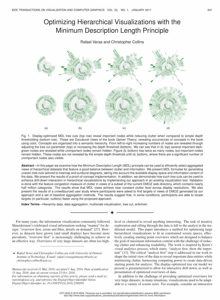
Fig. 1. Display-optimized MDL tree cuts (top row) reveal important nodes while reducing clutter when compared to simple depththresholding (bottom row). These are Docuburst views of the book Gamer Theory, revealing occurrences of concepts in the bookusing color. Concepts are organized into a semantic hierarchy. From left-to-right increasing numbers of nodes are revealed throughadjusting the tree cut parameter (top) or increasing the depth threshold (bottom). We can see that in (b, top) several important dark-green nodes are revealed while unimportant nodes remain hidden. Figure (b, bottom) has twice as many nodes, but important nodesremain hidden. These nodes are not revealed by the simple depth threshold until (d, bottom), where there are a significant number ofunimportant nodes also visible.
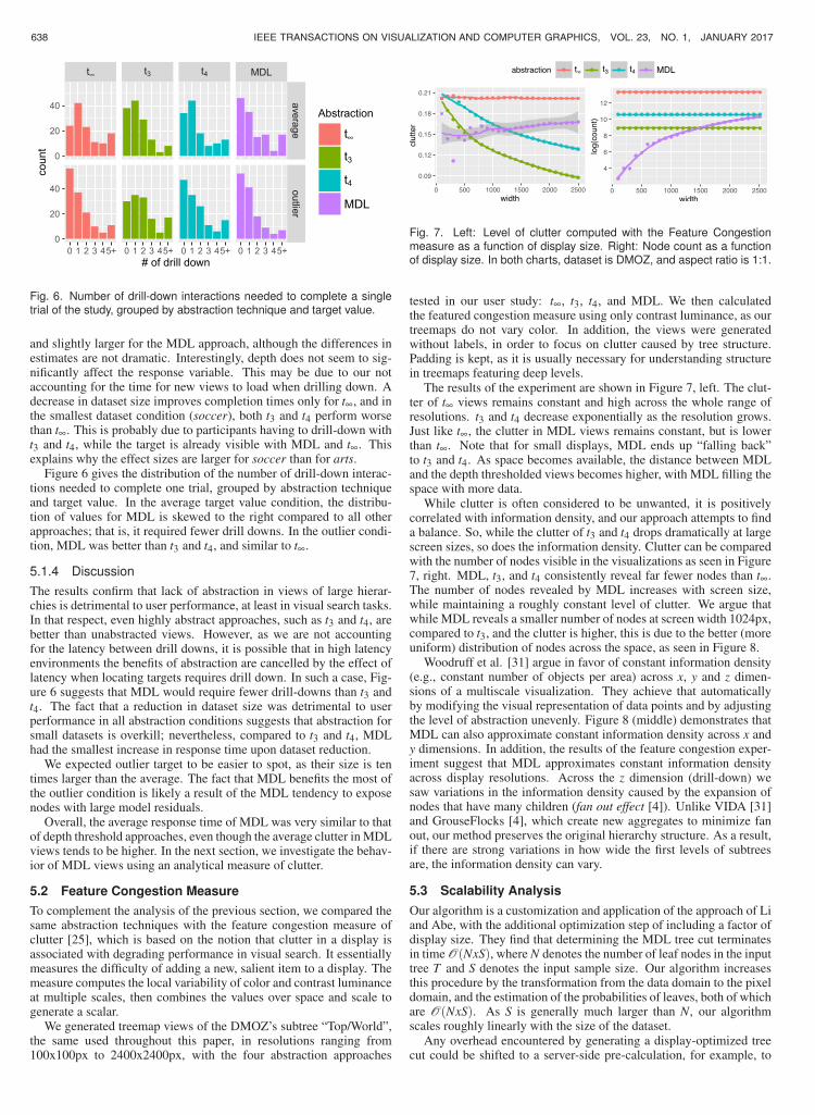
Abstract—In this paper we examine how the Minimum Description Length (MDL) principle can be used to efficiently select aggregatedviews of hierarchical datasets that feature a good balance between clutter and information. We present MDL formulae for generatinguneven tree cuts tailored to treemap and sunburst diagrams, taking into account the available display space and information content ofthe data. We present the results of a proof-of-concept implementation. In addition, we demonstrate how such tree cuts can be used toenhance drill-down interaction in hierarchical visualizations by implementing our approach in an existing visualization tool. Validationis done with the feature congestion measure of clutter in views of a subset of the current DMOZ web directory, which contains nearlyhalf million categories. The results show that MDL views achieve near constant clutter level across display resolutions. We alsopresent the results of a crowdsourced user study where participants were asked to find targets in views of DMOZ generated by ourapproach and a set of baseline aggregation methods. The results suggest that, in some conditions, participants are able to locatetargets (in particular, outliers) faster using the proposed approach.
Index Terms—Hierarchy data, data aggregation, multiscale visualization, tree cut, antichain
For many years, the information visualization community followedShneiderman’s celebrated visual information-seeking “mantra” for de-sign: “overview first, zoom and filter, details on demand” [27]. How-ever, as datasets have grown (and small displays have become moreprevalent), “overview first” is increasingly challenging to achieve inan effective way. Overviews of very large datasets are often too high-
• Rafael Veras and Christopher Collins are with University of OntarioInstitute of Technology. E-mail: [email protected];[email protected].
level or cluttered to reveal anything interesting. The task of iterativeexploration and sifting through the data is left to the analyst in the tra-ditional model. This paper introduces a method for optimizing largehierarchical visualizations to fit in constrained screen spaces, effec-tively creating starting point overviews which are designed to balancethe goal of maximum information content with the challenge of reduc-ing clutter and enhancing readability. The work is inspired by Keim’svisual analytics process, which starts: “analyze first, show the impor-tant” [13]. The critical “analyze first” step is addressed in our work toshape the initial view of the data to reveal important data entities whileminimizing clutter, harnessing computing power to create data-drivenstarting points for analysis. The display-optimized tree cut model wepresent is parameterized to allow for interactive drill down, as well aspresentation of optimized overviews of data.
In addition to the challenge of providing optimized overviews forvery large datasets, in many situations, visualizations need to be adapt-able to a variety of screen sizes. For example, consider an interactive
632 IEEE TRANSACTIONS ON VISUALIZATION AND COMPUTER GRAPHICS, VOL. 23, NO. 1, JANUARY 2017
visualization embedded as part of an online news story — one ver-sion may be appropriate for a smart phone display, while another willbe appropriate for a large monitor. The situation is not as simple aschanging the zoom factor, or the flow of the webpage, but rather thelevel of abstraction must adjust to make the visualization readable andaesthetically pleasing across devices.
Many factors influence the ability of visualization systems to ef-fectively display large amounts of data; in particular, the availabledisplay size, which is determined by the physical constraints of thescreen, and the perceptual scalability of the visualization, which de-pends on the choice of visual representation and layout [33]. Mostinformation visualizations become over-cluttered when the dataset islarge. Clutter reduction is an active area of research in information vi-sualization, as elaborated by Ellis and Dix in their taxonomy of clutterreduction methods [10]. Clutter is shown to have a negative impact onvisual search [12, 25, 30] and short term memory [20]. In a study oforientation judgment, Baldassi et al. found that clutter causes an in-crease in orientation judgment errors, and increase in perceived signalstrength and decision confidence on erroneous trials [5]. Rosenholtzet al. [26] include the notion of performance in the very definition ofclutter: a state in which excess items, or their representation or orga-nization, lead to degradation of performance at some task. Besides,in some resource-constrained client environments (e.g., web browser),the number of graphic primitives necessary to represent large data af-fects rendering and, consequently, interactive tasks, such as selectionand filtering.
In visualizations of hierarchical data, one can take advantage of thehierarchical structure to abstract data at varying levels, in order to re-duce the level of clutter when the available space prevents depictionof the full data. Visualizations that implement such strategy are calledmultiscale visualizations [11] and deciding the appropriate level of ab-straction for them is not trivial. Overly-detailed views have high clut-ter, whereas overly-abstract views can hide important patterns. Theright level of abstraction depends on the dataset and the available dis-play space; for example, large desktop displays afford more detail,while mobile phones have not only less space, but also coarser inter-action resolution due to the fat finger problem. In this paper, we referto this problem as the level of abstraction problem.
Our display-optimized MDL tree cut technique can be applied toany hierarchical dataset where there are quantitative data values asso-ciated with the leaves of the tree. In this paper we will introduce themathematical foundation behind our general display-optimized treecut, and demonstrate the approach applied to two popular hierarchi-cal visualization types — treemap and sunburst. Furthermore, we re-port on multiple validation approaches: a crowdsourced study in whichwe found that the tree cut approach provides for faster target findingcompared to traditional approaches, and a quantitative comparison ofclutter and information content across traditional techniques and ourdisplay-optimized MDL treemaps.
1 RELATED WORK
In this section, we survey two areas: techniques for controlling clutterin visualizations using aggregation and the use of tree cuts (also knownas antichains) to navigate large graph hierarchies.
1.1 Clutter Control
Based on the cartographic principle of constant information density[28], VIDA is a system that automatically creates visualizations inwhich density remains constant across zoom levels (z dimension) andwithin each view (x and y dimensions) [31]. The display is dividedinto regions, where the visual representation is modified (e.g., dots in-stead of glyphs) to meet a target density value specified by the user.Density measures are number of objects and number of vertices perunit of display area.
ViSizer is a framework for resizing visualizations [32]. It employsa sophisticated image warping technique that scales important regionsuniformly and deforms less important regions. The significance mea-sure is a compound of Rosenholtz et al.’s perception-based clutter mea-
sure [25] and a degree of interest (DOI) function. ViSizer focuses onnon-space filling visualizations such as word clouds and scatterplots.
Chuah [7] employs a simple strategy for automatic aggregation inhistograms, and ordered radial and treemap visualizations: aggregateneighboring objects whenever there is occlusion or they are too smallto be perceived. This approach works better where data items have anintuitive order (e.g., time series, histograms, or file directories orderedby name). Cui et al. [9] tackled the optimal level of abstraction prob-lem, but focusing only on accuracy; that is, how well the abstracteddata represent the original dataset. They proposed two measures ofquality: the histogram difference measure and the nearest neighbormeasure, which were integrated into XmdvTool. As the measures donot account for the visual quality of the resulting visualization, the userdetermines the best view interactively, by tweaking the level of detailand comparing the quality measure values. Likewise, based on aggre-gation quality measures, Andrienko and Andrienko [2] allow users tospecify the desired level of abstraction in visualizations of movementdata (flow maps).
Koutra et al. [14] proposed a parameter-free method based on theminimum description length to select the best (most succinct) sum-mary for large graphs among a set of alternatives: cliques, stars,chains, and bipartite cores.
Perhaps the closest to this proposal, Lamarche-Perrin et al. [15, 16]introduce a method for selecting abstract representations of hierarchi-cal datasets. In their work, a two-part information criteria consisting ofentropy and Kullback-Leibler divergence is used to select the tree cutfeaturing the best balance between conciseness and accuracy. Theirprocedure requires tuning a free weighting parameter that specifies therelative importance of one criterion over the other. It does not accountfor the available display space, so any adjustments to accommodatesmall or big screens need to be done manually by tuning the afore-mentioned weighting parameter.
1.2 Tree Cuts or Antichains
Tree cuts, also known as antichains, have been widely used in the ex-ploration of large graphs and hierarchies. SentireCrowds [6] and The-meCrowds [3] employ a maximal antichain selection method to ab-stract a hierarchy of topics visualized as a treemap. That method isbased on matching node scores resulting from user queries. Grouse-Flocks [4] reduces the complexity of interacting with large graphs byletting users manipulate cuts of superimposed aggregate hierarchies.Users can adjust the cut level of abstraction by performing topology-preserving operations involving merging and deletion of aggregates.In order to ensure the abstracted hierarchy view remains under the dis-play capacity, ASK-GraphView [1] parametrizes clustering with max-imum antichain size. In ASK-GraphView and GrouseFlocks the hi-erarchies are not part of the data, but created by an algorithm. Thisallows great flexibility to modify the hierarchy structure around dis-play constraints. In this work, we focus on “rigid” hierarchies, whereclasses carry domain specific relevance and, thus, cannot be merged ordeleted without cost to interpretation.
2 THEORETICAL FOUNDATIONS
Suppose a set of measurements D = (x1,y1), ..,(xn,yn) was collectedas part of an experiment and we were asked to send this data over anetwork where the transmission cost is high. Among the countlesspossible ways of encoding the data, it is in our best interest choosing ascheme that allows for the shortest message. In this scenario, the codelength for sending the raw data, assuming that encoding a number hasa fixed cost of b bits is:
L(D) =n
∑i=1
{L(xi)+L(yi)
}= 2nb. (1)
If the relation between x and y can be described by a polynomialmodel (or any other model), it might be possible to reduce significantlythe code length. As an example, let’s examine the polynomial case. A
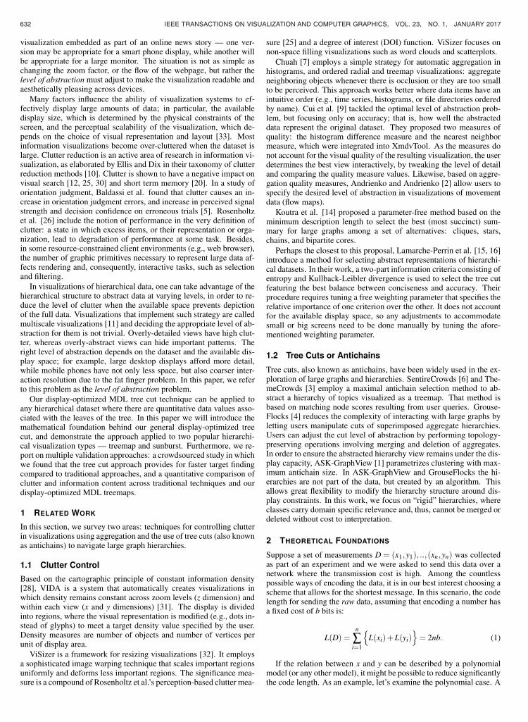
Fig. 2. On the left, a series of polynomials ranging from order 1 to 8fitted to a 10-point data set. On the right, the cost of encoding (in bits)the two parts of each polynomial model.
polynomial regression model has the following form:
y =p
∑k=0
akxk + ε. (2)
So the code length of the data as seen through a fitted polynomialmodel θ is:
L(θ ,D) =n
∑i=1
L(xi)+p
∑k=0
L(ak)+n
∑i=1
L(ri | θ), (3)
where ak is the k-th parameter of the polynomial and ri is the i-thresidual. Namely, the equation above is a sum of the cost of encodingthe model and the cost of encoding the data conditioned on the model(residuals). Note that the cost of sending the vector x is constant acrossall models. As a polynomial might not fit the data perfectly, it is neces-sary to send the model residuals, so that the receiver is able to recon-struct D accurately. However, depending on our tolerance to errors,we might be willing to ignore residuals smaller than a fixed threshold.The better the fit, the more economical is the description of the resid-uals. Overall, it is only worth representing our data with a polynomialmodel if we can find a model whose code length overhead is smallerthan the code length of vector y:
∑L(yi)> ∑L(ak)+∑L(ri|θ). (4)
To illustrate this notion, consider the ten data points depicted in Fig-ure 2, left. We fitted to this data a family of polynomials of increasingorder and compared the cost of representing the data with each of themin a setting where any number is represented with 64 bits, and residu-als smaller than 0.5 are ignored. Figure 2, right, shows the cost of eachfitted polynomial from order 1 to 8. It is clear that the more parametersa model has, the better is its fit. However, the model that provides theshortest description is that featuring the best balance between good-ness of fit and complexity. In our example, this model is the 4th orderpolynomial, which also satisfies (4), as the cost of encoding y in thenaive scheme is 640 bits.
In this example, we used information theoretic tools to determinethe model that most concisely captures the regularities in the data. Thecriterion we employed is a simplification of the Minimum DescriptionLength (MDL) Principle, which we describe formally in the followingsubsection. MDL is a powerful approach to model selection that hasbeen used to solve a large variety of problems, including polynomialregression, Gaussian density mixtures and Fourier series regression[17], and applied problems such as image segmentation [18], learningword association norms [19] and learning decision trees [22].
2.1 Minimum Description LengthProposed by Rissanen, MDL is an information criterion used formodel selection in statistics [23]. The principle is based on the follow-ing notion: given a set of observed data and a family of fitted models,the best model should provide the shortest encoding of the data. The
description length of a model is calculated as a sum of two parts: thelength of the binary codes that describe a) the model parameters, andb) the data residuals [18]. More formally, the MDL criterion can bewritten as:
L(θ ,x) = L(θ)+L(x | θ), (5)
where θ is a parameter vector, x is the data, and L(θ) and L(x | θ) arethe parameter description length (a) and the data description length(b), respectively.
Unlike in the polynomial example, where we used computer-oriented calculations for the code length, MDL is concerned with op-timal code length. That is, with MDL, we do not care about how amodel is encoded in practice as much as we care about how conciselyit can be encoded in theory. Let A be an alphabet and α be any of thesymbols in A. If the probability p(α) of occurrence of α ∈ A is known,then in the optimal encoding scheme for A the length of α is:
LOPT (α) =− log2 p(α). (6)
This result is important because often the likelihood function of themodel θ is known, so the data description length (number of bits toencode the residuals) follows from (6):
L(x | θ) =− log2 p(x | θ). (7)
For instance, in our polynomial example we could leverage the factthat, as per the regression model assumption, the residuals are approx-imately normally distributed, and use the log of the Gaussian likeli-hood, given by (n/2)log2(RSS/n), as L(x | θ), where RSS is the resid-ual sum of squares.
Frequently, the probability distribution of the model parameters(usually, a vector of integer or real numbers) is not given; in this case,Rissanen [23] proposes a universal prior probability distribution or,equivalently, a coding system, for integers. Rissanen demonstratedthat the optimal code length for such integers with unknown probabil-ity function can be achieved with his coding system and approximatedto log2n. Therefore, we can estimate the description length of arbitrar-ily complex models, as long as their parameters can be described asarrays of integers or real numbers.
Let’s assume θ is a vector of real numbers, which can be encoded byrepresenting the integer and fractional parts separately. The fractionalpart needs to be truncated to a pre-defined binary precision ρ , sincethe binary representation of many numbers can be infinite. Thus, thenumber of bits to encode θ is:
L(θ) =k
∑i=1
log2�θi�+ kρ, (8)
where k is the number of parameters in the model.Note that the choice of the precision ρ is of major importance.
Choosing fewer bits to encode the fractional parts yields a small L(θ),but at the expense of L(x | θ), as the residuals will be larger. A finerprecision reduces the residuals, as the encoded values will be closer tothe true estimates, but increases the cost of encoding the parameters. Inorder to minimize the description length, we need to optimize the pre-cision. Rissanen [24] shows that if the model parameters are estimatedfrom n data points using Maximum Likelihood Estimation (MLE) andn is large, the optimal precision ρ is approximately (log2 n)/2. Thus,(8) can be rewritten as:
L(θ) =k
∑i=1
log2�θi�+k2
log2 n. (9)
With the expressions for data and parameter description length, (5)can be written in more detail as:
L(θ ,x) =k
∑i=1
log2�θi�+k2
log2 n− log2 p(x | θ). (10)
VERAS AND COLLINS: OPTIMIZING HIERARCHICAL VISUALIZATIONS WITH THE MINIMUM DESCRIPTION LENGTH PRINCIPLE 633
visualization embedded as part of an online news story — one ver-sion may be appropriate for a smart phone display, while another willbe appropriate for a large monitor. The situation is not as simple aschanging the zoom factor, or the flow of the webpage, but rather thelevel of abstraction must adjust to make the visualization readable andaesthetically pleasing across devices.
Many factors influence the ability of visualization systems to ef-fectively display large amounts of data; in particular, the availabledisplay size, which is determined by the physical constraints of thescreen, and the perceptual scalability of the visualization, which de-pends on the choice of visual representation and layout [33]. Mostinformation visualizations become over-cluttered when the dataset islarge. Clutter reduction is an active area of research in information vi-sualization, as elaborated by Ellis and Dix in their taxonomy of clutterreduction methods [10]. Clutter is shown to have a negative impact onvisual search [12, 25, 30] and short term memory [20]. In a study oforientation judgment, Baldassi et al. found that clutter causes an in-crease in orientation judgment errors, and increase in perceived signalstrength and decision confidence on erroneous trials [5]. Rosenholtzet al. [26] include the notion of performance in the very definition ofclutter: a state in which excess items, or their representation or orga-nization, lead to degradation of performance at some task. Besides,in some resource-constrained client environments (e.g., web browser),the number of graphic primitives necessary to represent large data af-fects rendering and, consequently, interactive tasks, such as selectionand filtering.
In visualizations of hierarchical data, one can take advantage of thehierarchical structure to abstract data at varying levels, in order to re-duce the level of clutter when the available space prevents depictionof the full data. Visualizations that implement such strategy are calledmultiscale visualizations [11] and deciding the appropriate level of ab-straction for them is not trivial. Overly-detailed views have high clut-ter, whereas overly-abstract views can hide important patterns. Theright level of abstraction depends on the dataset and the available dis-play space; for example, large desktop displays afford more detail,while mobile phones have not only less space, but also coarser inter-action resolution due to the fat finger problem. In this paper, we referto this problem as the level of abstraction problem.
Our display-optimized MDL tree cut technique can be applied toany hierarchical dataset where there are quantitative data values asso-ciated with the leaves of the tree. In this paper we will introduce themathematical foundation behind our general display-optimized treecut, and demonstrate the approach applied to two popular hierarchi-cal visualization types — treemap and sunburst. Furthermore, we re-port on multiple validation approaches: a crowdsourced study in whichwe found that the tree cut approach provides for faster target findingcompared to traditional approaches, and a quantitative comparison ofclutter and information content across traditional techniques and ourdisplay-optimized MDL treemaps.
1 RELATED WORK
In this section, we survey two areas: techniques for controlling clutterin visualizations using aggregation and the use of tree cuts (also knownas antichains) to navigate large graph hierarchies.
1.1 Clutter Control
Based on the cartographic principle of constant information density[28], VIDA is a system that automatically creates visualizations inwhich density remains constant across zoom levels (z dimension) andwithin each view (x and y dimensions) [31]. The display is dividedinto regions, where the visual representation is modified (e.g., dots in-stead of glyphs) to meet a target density value specified by the user.Density measures are number of objects and number of vertices perunit of display area.
ViSizer is a framework for resizing visualizations [32]. It employsa sophisticated image warping technique that scales important regionsuniformly and deforms less important regions. The significance mea-sure is a compound of Rosenholtz et al.’s perception-based clutter mea-
sure [25] and a degree of interest (DOI) function. ViSizer focuses onnon-space filling visualizations such as word clouds and scatterplots.
Chuah [7] employs a simple strategy for automatic aggregation inhistograms, and ordered radial and treemap visualizations: aggregateneighboring objects whenever there is occlusion or they are too smallto be perceived. This approach works better where data items have anintuitive order (e.g., time series, histograms, or file directories orderedby name). Cui et al. [9] tackled the optimal level of abstraction prob-lem, but focusing only on accuracy; that is, how well the abstracteddata represent the original dataset. They proposed two measures ofquality: the histogram difference measure and the nearest neighbormeasure, which were integrated into XmdvTool. As the measures donot account for the visual quality of the resulting visualization, the userdetermines the best view interactively, by tweaking the level of detailand comparing the quality measure values. Likewise, based on aggre-gation quality measures, Andrienko and Andrienko [2] allow users tospecify the desired level of abstraction in visualizations of movementdata (flow maps).
Koutra et al. [14] proposed a parameter-free method based on theminimum description length to select the best (most succinct) sum-mary for large graphs among a set of alternatives: cliques, stars,chains, and bipartite cores.
Perhaps the closest to this proposal, Lamarche-Perrin et al. [15, 16]introduce a method for selecting abstract representations of hierarchi-cal datasets. In their work, a two-part information criteria consisting ofentropy and Kullback-Leibler divergence is used to select the tree cutfeaturing the best balance between conciseness and accuracy. Theirprocedure requires tuning a free weighting parameter that specifies therelative importance of one criterion over the other. It does not accountfor the available display space, so any adjustments to accommodatesmall or big screens need to be done manually by tuning the afore-mentioned weighting parameter.
1.2 Tree Cuts or Antichains
Tree cuts, also known as antichains, have been widely used in the ex-ploration of large graphs and hierarchies. SentireCrowds [6] and The-meCrowds [3] employ a maximal antichain selection method to ab-stract a hierarchy of topics visualized as a treemap. That method isbased on matching node scores resulting from user queries. Grouse-Flocks [4] reduces the complexity of interacting with large graphs byletting users manipulate cuts of superimposed aggregate hierarchies.Users can adjust the cut level of abstraction by performing topology-preserving operations involving merging and deletion of aggregates.In order to ensure the abstracted hierarchy view remains under the dis-play capacity, ASK-GraphView [1] parametrizes clustering with max-imum antichain size. In ASK-GraphView and GrouseFlocks the hi-erarchies are not part of the data, but created by an algorithm. Thisallows great flexibility to modify the hierarchy structure around dis-play constraints. In this work, we focus on “rigid” hierarchies, whereclasses carry domain specific relevance and, thus, cannot be merged ordeleted without cost to interpretation.
2 THEORETICAL FOUNDATIONS
Suppose a set of measurements D = (x1,y1), ..,(xn,yn) was collectedas part of an experiment and we were asked to send this data over anetwork where the transmission cost is high. Among the countlesspossible ways of encoding the data, it is in our best interest choosing ascheme that allows for the shortest message. In this scenario, the codelength for sending the raw data, assuming that encoding a number hasa fixed cost of b bits is:
L(D) =n
∑i=1
{L(xi)+L(yi)
}= 2nb. (1)
If the relation between x and y can be described by a polynomialmodel (or any other model), it might be possible to reduce significantlythe code length. As an example, let’s examine the polynomial case. A
Fig. 2. On the left, a series of polynomials ranging from order 1 to 8fitted to a 10-point data set. On the right, the cost of encoding (in bits)the two parts of each polynomial model.
polynomial regression model has the following form:
y =p
∑k=0
akxk + ε. (2)
So the code length of the data as seen through a fitted polynomialmodel θ is:
L(θ ,D) =n
∑i=1
L(xi)+p
∑k=0
L(ak)+n
∑i=1
L(ri | θ), (3)
where ak is the k-th parameter of the polynomial and ri is the i-thresidual. Namely, the equation above is a sum of the cost of encodingthe model and the cost of encoding the data conditioned on the model(residuals). Note that the cost of sending the vector x is constant acrossall models. As a polynomial might not fit the data perfectly, it is neces-sary to send the model residuals, so that the receiver is able to recon-struct D accurately. However, depending on our tolerance to errors,we might be willing to ignore residuals smaller than a fixed threshold.The better the fit, the more economical is the description of the resid-uals. Overall, it is only worth representing our data with a polynomialmodel if we can find a model whose code length overhead is smallerthan the code length of vector y:
∑L(yi)> ∑L(ak)+∑L(ri|θ). (4)
To illustrate this notion, consider the ten data points depicted in Fig-ure 2, left. We fitted to this data a family of polynomials of increasingorder and compared the cost of representing the data with each of themin a setting where any number is represented with 64 bits, and residu-als smaller than 0.5 are ignored. Figure 2, right, shows the cost of eachfitted polynomial from order 1 to 8. It is clear that the more parametersa model has, the better is its fit. However, the model that provides theshortest description is that featuring the best balance between good-ness of fit and complexity. In our example, this model is the 4th orderpolynomial, which also satisfies (4), as the cost of encoding y in thenaive scheme is 640 bits.
In this example, we used information theoretic tools to determinethe model that most concisely captures the regularities in the data. Thecriterion we employed is a simplification of the Minimum DescriptionLength (MDL) Principle, which we describe formally in the followingsubsection. MDL is a powerful approach to model selection that hasbeen used to solve a large variety of problems, including polynomialregression, Gaussian density mixtures and Fourier series regression[17], and applied problems such as image segmentation [18], learningword association norms [19] and learning decision trees [22].
2.1 Minimum Description LengthProposed by Rissanen, MDL is an information criterion used formodel selection in statistics [23]. The principle is based on the follow-ing notion: given a set of observed data and a family of fitted models,the best model should provide the shortest encoding of the data. The
description length of a model is calculated as a sum of two parts: thelength of the binary codes that describe a) the model parameters, andb) the data residuals [18]. More formally, the MDL criterion can bewritten as:
L(θ ,x) = L(θ)+L(x | θ), (5)
where θ is a parameter vector, x is the data, and L(θ) and L(x | θ) arethe parameter description length (a) and the data description length(b), respectively.
Unlike in the polynomial example, where we used computer-oriented calculations for the code length, MDL is concerned with op-timal code length. That is, with MDL, we do not care about how amodel is encoded in practice as much as we care about how conciselyit can be encoded in theory. Let A be an alphabet and α be any of thesymbols in A. If the probability p(α) of occurrence of α ∈ A is known,then in the optimal encoding scheme for A the length of α is:
LOPT (α) =− log2 p(α). (6)
This result is important because often the likelihood function of themodel θ is known, so the data description length (number of bits toencode the residuals) follows from (6):
L(x | θ) =− log2 p(x | θ). (7)
For instance, in our polynomial example we could leverage the factthat, as per the regression model assumption, the residuals are approx-imately normally distributed, and use the log of the Gaussian likeli-hood, given by (n/2)log2(RSS/n), as L(x | θ), where RSS is the resid-ual sum of squares.
Frequently, the probability distribution of the model parameters(usually, a vector of integer or real numbers) is not given; in this case,Rissanen [23] proposes a universal prior probability distribution or,equivalently, a coding system, for integers. Rissanen demonstratedthat the optimal code length for such integers with unknown probabil-ity function can be achieved with his coding system and approximatedto log2n. Therefore, we can estimate the description length of arbitrar-ily complex models, as long as their parameters can be described asarrays of integers or real numbers.
Let’s assume θ is a vector of real numbers, which can be encoded byrepresenting the integer and fractional parts separately. The fractionalpart needs to be truncated to a pre-defined binary precision ρ , sincethe binary representation of many numbers can be infinite. Thus, thenumber of bits to encode θ is:
L(θ) =k
∑i=1
log2�θi�+ kρ, (8)
where k is the number of parameters in the model.Note that the choice of the precision ρ is of major importance.
Choosing fewer bits to encode the fractional parts yields a small L(θ),but at the expense of L(x | θ), as the residuals will be larger. A finerprecision reduces the residuals, as the encoded values will be closer tothe true estimates, but increases the cost of encoding the parameters. Inorder to minimize the description length, we need to optimize the pre-cision. Rissanen [24] shows that if the model parameters are estimatedfrom n data points using Maximum Likelihood Estimation (MLE) andn is large, the optimal precision ρ is approximately (log2 n)/2. Thus,(8) can be rewritten as:
L(θ) =k
∑i=1
log2�θi�+k2
log2 n. (9)
With the expressions for data and parameter description length, (5)can be written in more detail as:
L(θ ,x) =k
∑i=1
log2�θi�+k2
log2 n− log2 p(x | θ). (10)
634 IEEE TRANSACTIONS ON VISUALIZATION AND COMPUTER GRAPHICS, VOL. 23, NO. 1, JANUARY 2017
L(A) < L(B)L(A | S) > L(B | S)
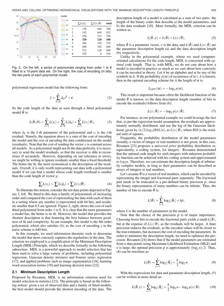
Fig. 3. An illustration of two tree cuts. More abstract cuts have lowerparameter description length, but higher data description length.
Equation 10 embodies the fundamental trade-off between concise-ness and accuracy that defines the MDL principle. Models with moreparameters will achieve better accuracy (high likelihood) at the ex-pense of simplicity. In fact, if we set L(θ) constant, MDL falls backto MLE, selecting the model that offers the best fit to the data. Inthat sense, L(θ) can be thought of as a safeguard against over-fitting.Likewise, over-concise models have low accuracy, being just as un-desirable. Minimization of the description length tends to select themodel featuring the best balance between these criteria. In the infor-mation theoretic interpretation, the selected model corresponds to thebest compression of the data.
2.2 MDL Tree Cut ModelHaving laid out the general formulation of the MDL principle, in thissection we explain the tree cut model, which is an important buildingblock for our abstraction approach. The tree cut model is a general-ization method based on MDL, originally developed for the linguisticproblem of automatic acquisition of case frame patterns from largecorpora [19].
Consider a tree structure representing the hierarchical relation be-tween abstract classes, e.g., IS-A, part of, instance of. The degree ofabstraction grows towards the root. Assume that only the leaves areobservable (countable), and the internal nodes accumulate the countsof their children. L is the set of all leaves. A dataset S is a multisetof observations, each representing one occurrence of a leaf l ∈ L, withl ∈ S denoting the inclusion of l in S as a multiset. We denote thedataset size by |S|, the total number of observations.
A tree cut is any set of tree nodes that exhaustively covers the leafnodes. Graphically, it can be represented by a path crossing the treelengthwise, as in Figure 3. Nodes along the cut represent the subtreesdominated by them and are assigned each a probability value. De-pending on how regular is our data S, a concise way to transmit it overan arbitrary channel to a receiver who has knowledge of the tree is tosend a tree cut. The receiver then estimates the value of each leaf basedon the value of the node representing it in the cut. In other words, acut is a model of the data, carrying estimates of the observed values.The residuals are sent separately, in the MDL fashion, as discussed inSection 2.1.
A tree cut model M is defined as the tuple (Γ , θ), where Γ =
[C1,C2, ...,Ck] and θ = [P(C1), P(C2), ..., P(Ck)]: the vector of nodes(classes) and their parameters (estimated probabilities), respectively.The probability P(C) of a class is estimated by MLE, as follows:
P(C) =f (C)
|S|, (11)
where f (C) is the accumulated count of the class C. The estimatedprobability of each of the leaves under a class is obtained by normal-ization of the class probability over the number of leaves C under theclass:
P(l) =P(C)
|C|. (12)
Note that behind this formula is the assumption of uniform probabil-ity. This means the probabilities (or frequencies) of the leaves undera cut are smoothed, reflecting the decrease in uncertainty when data isrepresented by abstract models.
As discussed in the previous section, the data description length isthe log of the likelihood of the data:
L(S |Γ , θ) =−∑l∈S
log2 P(l). (13)
The minimum data description length is held by the deepest tree cutmodel, comprised of all leaves, which features no better abstractionthan the raw data. The cost of encoding the parameters θ of the model,an array of real numbers, is given by (9). Note that, Li & Abe omitthe first term in (9), namely, the cost of encoding the integer part ofthe parameters, because the model parameters are probabilities; hence,the cost of encoding the integer parts is always 0. In summary, Li andAbe’s tree cut model minimizes the following information criterion:
L(θ ,S) =k2
log2 |S|−∑l∈S
log2 P(l). (14)
To be more precise, in addition to the probabilities θ , a receiverwould also need to know the classes Γ to decode the data correctly.Since the number of possible cuts in a tree is finite, in theory we coulduse an index to inform Γ , as part of the coding scheme. As suchindexes would be equally probable a priori, their code length wouldbe constant for all models and so, can be safely ignored. For sake ofmodel selection, all we need to account for is the cost of encoding θand (S | θ).
Li and Abe provided an efficient and simple bottom up algorithm,based on dynamic programming, that is guaranteed to find the tree cutwhose description length is minimal [19]. In the rest of this paper,we present different ways to calculate parameter and data descriptionlengths, but the same algorithm is used for minimization.
3 MDL DRILL-DOWN
In this section, we experiment with using the tree cuts selected by Liand Abe’s approach to inform which nodes should be abstracted inviews of a hierarchical dataset. Since such cuts are generated with noconsideration of the available display size, we adapt the method byintroducing a weighting parameter that determines the relative impor-tance of fitness to the data over clutter. An increase in weight resultsin a deeper tree cut. In our proof-of-concept, the user can manipulatethis parameter seamlessly through conventional drill-down to increasethe level of detail of the view.
We chose to implement the technique on Docuburst, an open-sourcedocument visualization tool [8]. Docuburst displays a sunburst repre-sentation of the WordNet ontology where the size of nodes and cat-egories (angular extent) is weighted by their occurrence in the inputdocument, allowing users to inspect which words and categories ofwords are more prevalent in a document. The color of a node is basedon the non-cumulative count of uses of the corresponding word in thedocument. In their future work section, Collins et al. discuss twoproblems that could potentially be solved with uneven MDL tree cuts.First, abstracting subtrees that have low relative importance. Second,the top levels of WordNet are too abstract, as far as carrying little in-formation about the document’s content.
Figure 1 features views of the book Gamer Theory, by McKen-zie Wark. The most representative categories of the document are thedarkest (most frequent); for instance: game, entertainment, algorithm,storyline, boredom, etc. In a full tree view, 6,302 nodes would berendered, which is likely enough to cause latency in a browser-basedvisualization. Also, displaying this many nodes results in small, illeg-ible labels and the need to interactively zoom and pan.
The tree cut resulting from minimizing Li and Abe’s informationcriterion is shown in Figure 1(a). Nodes under the tree cut are hidden,whereas nodes on or above the tree cut are visible. Unless the availabledisplay size is limited, that view can be considered too abstract.
Following Wagner [29], we introduce a free weighting parameter Wto equation (14) as a means to control the importance of the data de-scription length over the parameter description length and, as a result,the tree cut depth:
L(θ ,S) =k2
log2 |S|−W ∑l∈S
log2 P(l) (W > 0). (15)
The semantics of increasing W is equivalent to that of drilling down;the more weight applied to the data description length (residuals), themore parameters (nodes) will be included in the model (tree cut), tominimize the overall description length. Thus, weighted MDL treecuts can be useful to reveal details at a rate that is more compatiblewith the distribution of values in the hierarchy. In order to illustratethis concept, we mapped W to the drill-down action in Docuburst; thatis, when users roll the mouse wheel, W is incremented/decremented bya predefined delta. Figure 1(b-d), top, shows the result of three sub-sequent increments in W , starting from 1(a), top. In contrast, Figure1(b-d), bottom, shows the result of three drill-down steps where a con-ventional depth threshold is incremented. It is clear that, in only a fewsteps, weighted MDL views allow access to most of the representa-tive nodes in the document with much less clutter than using the depththreshold or the full overview. In terms of number of nodes rendered(a-d), the weighted MDL views cost 32, 387, 730, and 887 nodes;while the depth threshold views cost 183, 808, 2202, 4199 nodes.
An important concern is choosing ∆W so that every increment re-sults in a view that has significantly more information than the pre-vious. In our tests, ∆W was defined empirically, and a value of 250yielded good results for visualizing a variety of documents.
Weighted MDL views can be useful as a way to explore visualiza-tions interactively, but the problem of optimizing the level of detail as afunction of the available display space before any user input remainedunsolved. Specifically, we needed a method capable of generating afirst view of the dataset that is as informative as possible within thebounds of readability. Next section presents a satisfactory method.
4 DISPLAY-TAILORED TREE CUT MODELS
We begin this section with the consideration that hierarchical visual-ization concerns, in general, the representation of tree cut models, inthe sense defined in Section 2.2. If we treat visualization techniques(e.g., treemap, sunburst) as coding schemes and the views producedwith them as encoded tree cut models, we can select optimal viewsusing MDL criteria. In particular, we are interested in expressing pa-rameter and data description lengths in a way that relates to clutter andfitness in visualizations. We will focus on space-filling hierarchicalvisualization techniques, as the connection to MDL is more obvious.
In a space-filling visual representation of a hierarchical dataset, thepixel grid is divided into areas proportional to the data values. Areasare recursively grouped in the visual space according to the hierarchytopology, so that siblings are always adjacent. In addition, color andlabels can be used to convey the hierarchical structure.
A non-aggregated hierarchical visualization Vmax is an encoding ofthe deepest tree cut model of a dataset. For example, in a treemapwithout decorations (e.g., padding), Vmax fills the entire display spacewith rectangles representing the tree leaves. Given the set Λ of visu-alizations of S using a specific layout, each of which corresponds to atree cut of S, Vmax is the visualization that maximizes L(V ):
Vmax = argmaxV∈Λ
(L(V )), (16)
where S denotes the dataset. Note that, for sake of simplicity, we makeno distinction in the notation between a visualization V and the tree cutencoded by it.
In the information theoretic interpretation, if visualizations allowedfor lossless coding, Vmax would always minimize L(S |V ) and pro-vide the best fit to the data, corresponding to the model selected byMDL when we set L(V ) constant or, equivalently, to the model se-lected by MLE. However, a space-filling visualization is a partial andlossy coding system: partial because there exist some source symbols
that cannot be encoded (e.g., data points that map to subpixel areas);lossy because it is possible that a pair of symbols share a code word(e.g., data points that map to overlapping areas due to rounding).
Depending on the available display space, when the dataset is rela-tively small, Vmax generally provides the best fit to the data, but whenthe number of leaves is large, decoding of information is impacted,due to the aforementioned limitations caused by display pixel reso-lution. This is a key departure from Li and Abe’s method, where anincrease in the length of the model always yields an increase in fitness.In other words, there is a limit on the model fitness to data achievableby a space-filling visualization. The fact that Vmax does not necessarilyhold the minimum data description length can be denoted as follows:
L(S |Vmax)≥ minV∈Λ
L(S |V ), (17)
This inequality can be read as: the data description length of thevisualization of the deepest tree cut (Vmax) is not necessarily minimal.As a result, before even considering the parameter description length,we can observe that it pays off selecting treemaps more abstract thanVmax when datasets are large relative to the available screen size.
4.1 Treemap
Let’s define the dataset S in more detail. S is a 2-tuple (L, f ), whereL is the subset of classes that are tree leaves, and f is a function suchthat for each l ∈ L, f (l) is the count of l.
Then the area of a leaf can be defined as the following compositefunction with respect to the display area D (in pixels):
(A◦ f )(l) = A( f (l)) =f (l)|S|
D. (18)
Likewise, the area of an abstract class C is given by:
A( f (C)) = ∑l∈C
A( f (l)), (19)
where l ∈ C is the set of tree leaves dominated by C. We call G =(L,A ◦ f ) the linearly transformed dataset using A ◦ f . Essentially, Gis the dataset with scores transformed to pixels. The probabilities ofthe classes are estimated based on the encoded G. For conciseness, weabbreviate A( f (C)) as A(C) in the rest of this section.
A treemap encodes such areas as a vector of rectangle coordinatesR = [R1,R2, ...,Rk]. Formally, we describe a treemap as a 2-tupleT = (Γ ,(R |D)). Given D, we can refer to any point in the grid with aninteger index 1 ≤ i ≤ D. Thus, to transmit Ri, we need only two inte-gers, corresponding to the indexes of the top left and bottom right cor-ners. Since the index space is finite and the indexes are equally likely,we can use Rissanen’s universal prior to arrive at L(i) = log2(D). Theparameter description length is then:
L(R) = 2k log2 D. (20)
Equation 20 gives an approximation of the optimal number of bitsnecessary to transmit the parameters of a treemap, ignoring any factorsthat are constant across all treemaps. For the sake of simplicity, weconsider a treemap with no colors or labels.
Since the pixel grid imposes a limited precision on the representa-tion of areas, we approximate the encoded area of C in the treemap byrounding A(C):
A′(C) = �A(C)+1/2�. (21)
Note that A′(C) does not account for precision lost by the fact thatA(C) has to be decomposable into exactly two factors. P(C) is esti-mated simply as the ratio between the encoded class area and the totaldisplay area:
P(C) =A′(C)
D. (22)
VERAS AND COLLINS: OPTIMIZING HIERARCHICAL VISUALIZATIONS WITH THE MINIMUM DESCRIPTION LENGTH PRINCIPLE 635
L(A) < L(B)L(A | S) > L(B | S)
Fig. 3. An illustration of two tree cuts. More abstract cuts have lowerparameter description length, but higher data description length.
Equation 10 embodies the fundamental trade-off between concise-ness and accuracy that defines the MDL principle. Models with moreparameters will achieve better accuracy (high likelihood) at the ex-pense of simplicity. In fact, if we set L(θ) constant, MDL falls backto MLE, selecting the model that offers the best fit to the data. Inthat sense, L(θ) can be thought of as a safeguard against over-fitting.Likewise, over-concise models have low accuracy, being just as un-desirable. Minimization of the description length tends to select themodel featuring the best balance between these criteria. In the infor-mation theoretic interpretation, the selected model corresponds to thebest compression of the data.
2.2 MDL Tree Cut ModelHaving laid out the general formulation of the MDL principle, in thissection we explain the tree cut model, which is an important buildingblock for our abstraction approach. The tree cut model is a general-ization method based on MDL, originally developed for the linguisticproblem of automatic acquisition of case frame patterns from largecorpora [19].
Consider a tree structure representing the hierarchical relation be-tween abstract classes, e.g., IS-A, part of, instance of. The degree ofabstraction grows towards the root. Assume that only the leaves areobservable (countable), and the internal nodes accumulate the countsof their children. L is the set of all leaves. A dataset S is a multisetof observations, each representing one occurrence of a leaf l ∈ L, withl ∈ S denoting the inclusion of l in S as a multiset. We denote thedataset size by |S|, the total number of observations.
A tree cut is any set of tree nodes that exhaustively covers the leafnodes. Graphically, it can be represented by a path crossing the treelengthwise, as in Figure 3. Nodes along the cut represent the subtreesdominated by them and are assigned each a probability value. De-pending on how regular is our data S, a concise way to transmit it overan arbitrary channel to a receiver who has knowledge of the tree is tosend a tree cut. The receiver then estimates the value of each leaf basedon the value of the node representing it in the cut. In other words, acut is a model of the data, carrying estimates of the observed values.The residuals are sent separately, in the MDL fashion, as discussed inSection 2.1.
A tree cut model M is defined as the tuple (Γ , θ), where Γ =
[C1,C2, ...,Ck] and θ = [P(C1), P(C2), ..., P(Ck)]: the vector of nodes(classes) and their parameters (estimated probabilities), respectively.The probability P(C) of a class is estimated by MLE, as follows:
P(C) =f (C)
|S|, (11)
where f (C) is the accumulated count of the class C. The estimatedprobability of each of the leaves under a class is obtained by normal-ization of the class probability over the number of leaves C under theclass:
P(l) =P(C)
|C|. (12)
Note that behind this formula is the assumption of uniform probabil-ity. This means the probabilities (or frequencies) of the leaves undera cut are smoothed, reflecting the decrease in uncertainty when data isrepresented by abstract models.
As discussed in the previous section, the data description length isthe log of the likelihood of the data:
L(S |Γ , θ) =−∑l∈S
log2 P(l). (13)
The minimum data description length is held by the deepest tree cutmodel, comprised of all leaves, which features no better abstractionthan the raw data. The cost of encoding the parameters θ of the model,an array of real numbers, is given by (9). Note that, Li & Abe omitthe first term in (9), namely, the cost of encoding the integer part ofthe parameters, because the model parameters are probabilities; hence,the cost of encoding the integer parts is always 0. In summary, Li andAbe’s tree cut model minimizes the following information criterion:
L(θ ,S) =k2
log2 |S|−∑l∈S
log2 P(l). (14)
To be more precise, in addition to the probabilities θ , a receiverwould also need to know the classes Γ to decode the data correctly.Since the number of possible cuts in a tree is finite, in theory we coulduse an index to inform Γ , as part of the coding scheme. As suchindexes would be equally probable a priori, their code length wouldbe constant for all models and so, can be safely ignored. For sake ofmodel selection, all we need to account for is the cost of encoding θand (S | θ).
Li and Abe provided an efficient and simple bottom up algorithm,based on dynamic programming, that is guaranteed to find the tree cutwhose description length is minimal [19]. In the rest of this paper,we present different ways to calculate parameter and data descriptionlengths, but the same algorithm is used for minimization.
3 MDL DRILL-DOWN
In this section, we experiment with using the tree cuts selected by Liand Abe’s approach to inform which nodes should be abstracted inviews of a hierarchical dataset. Since such cuts are generated with noconsideration of the available display size, we adapt the method byintroducing a weighting parameter that determines the relative impor-tance of fitness to the data over clutter. An increase in weight resultsin a deeper tree cut. In our proof-of-concept, the user can manipulatethis parameter seamlessly through conventional drill-down to increasethe level of detail of the view.
We chose to implement the technique on Docuburst, an open-sourcedocument visualization tool [8]. Docuburst displays a sunburst repre-sentation of the WordNet ontology where the size of nodes and cat-egories (angular extent) is weighted by their occurrence in the inputdocument, allowing users to inspect which words and categories ofwords are more prevalent in a document. The color of a node is basedon the non-cumulative count of uses of the corresponding word in thedocument. In their future work section, Collins et al. discuss twoproblems that could potentially be solved with uneven MDL tree cuts.First, abstracting subtrees that have low relative importance. Second,the top levels of WordNet are too abstract, as far as carrying little in-formation about the document’s content.
Figure 1 features views of the book Gamer Theory, by McKen-zie Wark. The most representative categories of the document are thedarkest (most frequent); for instance: game, entertainment, algorithm,storyline, boredom, etc. In a full tree view, 6,302 nodes would berendered, which is likely enough to cause latency in a browser-basedvisualization. Also, displaying this many nodes results in small, illeg-ible labels and the need to interactively zoom and pan.
The tree cut resulting from minimizing Li and Abe’s informationcriterion is shown in Figure 1(a). Nodes under the tree cut are hidden,whereas nodes on or above the tree cut are visible. Unless the availabledisplay size is limited, that view can be considered too abstract.
Following Wagner [29], we introduce a free weighting parameter Wto equation (14) as a means to control the importance of the data de-scription length over the parameter description length and, as a result,the tree cut depth:
L(θ ,S) =k2
log2 |S|−W ∑l∈S
log2 P(l) (W > 0). (15)
The semantics of increasing W is equivalent to that of drilling down;the more weight applied to the data description length (residuals), themore parameters (nodes) will be included in the model (tree cut), tominimize the overall description length. Thus, weighted MDL treecuts can be useful to reveal details at a rate that is more compatiblewith the distribution of values in the hierarchy. In order to illustratethis concept, we mapped W to the drill-down action in Docuburst; thatis, when users roll the mouse wheel, W is incremented/decremented bya predefined delta. Figure 1(b-d), top, shows the result of three sub-sequent increments in W , starting from 1(a), top. In contrast, Figure1(b-d), bottom, shows the result of three drill-down steps where a con-ventional depth threshold is incremented. It is clear that, in only a fewsteps, weighted MDL views allow access to most of the representa-tive nodes in the document with much less clutter than using the depththreshold or the full overview. In terms of number of nodes rendered(a-d), the weighted MDL views cost 32, 387, 730, and 887 nodes;while the depth threshold views cost 183, 808, 2202, 4199 nodes.
An important concern is choosing ∆W so that every increment re-sults in a view that has significantly more information than the pre-vious. In our tests, ∆W was defined empirically, and a value of 250yielded good results for visualizing a variety of documents.
Weighted MDL views can be useful as a way to explore visualiza-tions interactively, but the problem of optimizing the level of detail as afunction of the available display space before any user input remainedunsolved. Specifically, we needed a method capable of generating afirst view of the dataset that is as informative as possible within thebounds of readability. Next section presents a satisfactory method.
4 DISPLAY-TAILORED TREE CUT MODELS
We begin this section with the consideration that hierarchical visual-ization concerns, in general, the representation of tree cut models, inthe sense defined in Section 2.2. If we treat visualization techniques(e.g., treemap, sunburst) as coding schemes and the views producedwith them as encoded tree cut models, we can select optimal viewsusing MDL criteria. In particular, we are interested in expressing pa-rameter and data description lengths in a way that relates to clutter andfitness in visualizations. We will focus on space-filling hierarchicalvisualization techniques, as the connection to MDL is more obvious.
In a space-filling visual representation of a hierarchical dataset, thepixel grid is divided into areas proportional to the data values. Areasare recursively grouped in the visual space according to the hierarchytopology, so that siblings are always adjacent. In addition, color andlabels can be used to convey the hierarchical structure.
A non-aggregated hierarchical visualization Vmax is an encoding ofthe deepest tree cut model of a dataset. For example, in a treemapwithout decorations (e.g., padding), Vmax fills the entire display spacewith rectangles representing the tree leaves. Given the set Λ of visu-alizations of S using a specific layout, each of which corresponds to atree cut of S, Vmax is the visualization that maximizes L(V ):
Vmax = argmaxV∈Λ
(L(V )), (16)
where S denotes the dataset. Note that, for sake of simplicity, we makeno distinction in the notation between a visualization V and the tree cutencoded by it.
In the information theoretic interpretation, if visualizations allowedfor lossless coding, Vmax would always minimize L(S |V ) and pro-vide the best fit to the data, corresponding to the model selected byMDL when we set L(V ) constant or, equivalently, to the model se-lected by MLE. However, a space-filling visualization is a partial andlossy coding system: partial because there exist some source symbols
that cannot be encoded (e.g., data points that map to subpixel areas);lossy because it is possible that a pair of symbols share a code word(e.g., data points that map to overlapping areas due to rounding).
Depending on the available display space, when the dataset is rela-tively small, Vmax generally provides the best fit to the data, but whenthe number of leaves is large, decoding of information is impacted,due to the aforementioned limitations caused by display pixel reso-lution. This is a key departure from Li and Abe’s method, where anincrease in the length of the model always yields an increase in fitness.In other words, there is a limit on the model fitness to data achievableby a space-filling visualization. The fact that Vmax does not necessarilyhold the minimum data description length can be denoted as follows:
L(S |Vmax)≥ minV∈Λ
L(S |V ), (17)
This inequality can be read as: the data description length of thevisualization of the deepest tree cut (Vmax) is not necessarily minimal.As a result, before even considering the parameter description length,we can observe that it pays off selecting treemaps more abstract thanVmax when datasets are large relative to the available screen size.
4.1 Treemap
Let’s define the dataset S in more detail. S is a 2-tuple (L, f ), whereL is the subset of classes that are tree leaves, and f is a function suchthat for each l ∈ L, f (l) is the count of l.
Then the area of a leaf can be defined as the following compositefunction with respect to the display area D (in pixels):
(A◦ f )(l) = A( f (l)) =f (l)|S|
D. (18)
Likewise, the area of an abstract class C is given by:
A( f (C)) = ∑l∈C
A( f (l)), (19)
where l ∈ C is the set of tree leaves dominated by C. We call G =(L,A ◦ f ) the linearly transformed dataset using A ◦ f . Essentially, Gis the dataset with scores transformed to pixels. The probabilities ofthe classes are estimated based on the encoded G. For conciseness, weabbreviate A( f (C)) as A(C) in the rest of this section.
A treemap encodes such areas as a vector of rectangle coordinatesR = [R1,R2, ...,Rk]. Formally, we describe a treemap as a 2-tupleT = (Γ ,(R |D)). Given D, we can refer to any point in the grid with aninteger index 1 ≤ i ≤ D. Thus, to transmit Ri, we need only two inte-gers, corresponding to the indexes of the top left and bottom right cor-ners. Since the index space is finite and the indexes are equally likely,we can use Rissanen’s universal prior to arrive at L(i) = log2(D). Theparameter description length is then:
L(R) = 2k log2 D. (20)
Equation 20 gives an approximation of the optimal number of bitsnecessary to transmit the parameters of a treemap, ignoring any factorsthat are constant across all treemaps. For the sake of simplicity, weconsider a treemap with no colors or labels.
Since the pixel grid imposes a limited precision on the representa-tion of areas, we approximate the encoded area of C in the treemap byrounding A(C):
A′(C) = �A(C)+1/2�. (21)
Note that A′(C) does not account for precision lost by the fact thatA(C) has to be decomposable into exactly two factors. P(C) is esti-mated simply as the ratio between the encoded class area and the totaldisplay area:
P(C) =A′(C)
D. (22)
636 IEEE TRANSACTIONS ON VISUALIZATION AND COMPUTER GRAPHICS, VOL. 23, NO. 1, JANUARY 2017
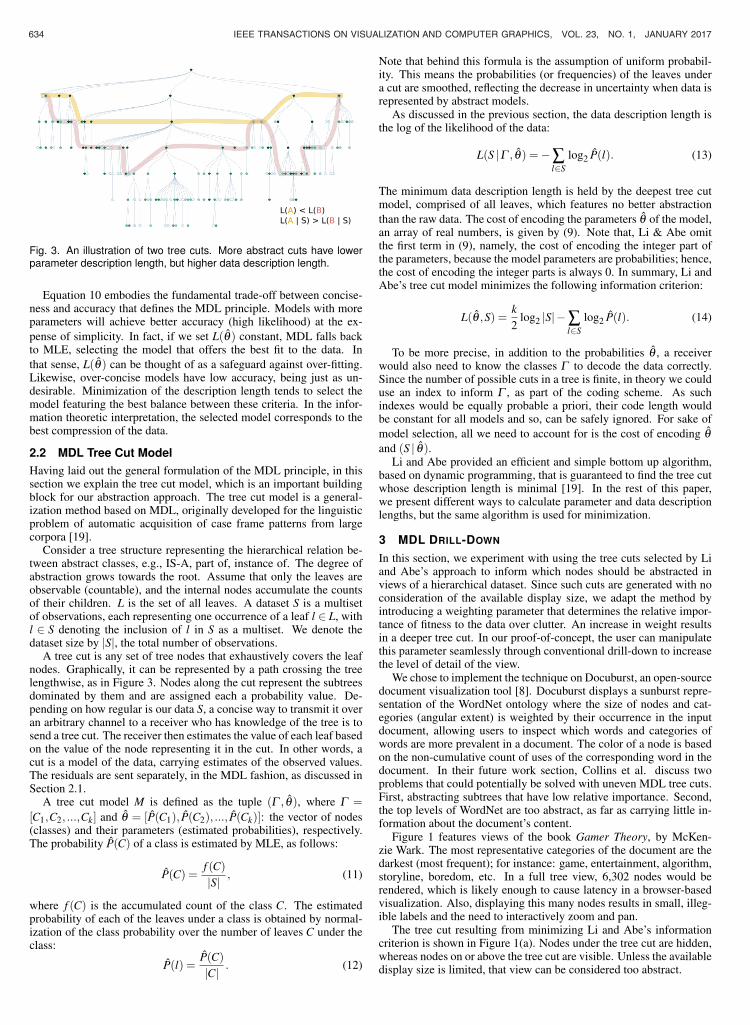
Fig. 4. Treemap visualizations generated with the display-tailored MDL procedure, with the following resolutions: 375x400px, 375x667px and1920x1080px. More abstract tree cuts are selected for smaller displays.
As in (12), we assume that P(l) is estimated by normalizing P(C)with respect to the leaves dominated by C:
P(l) =
{P(C)|C| if P(C)> 0
c if P(C) = 0(23)
where c is a constant representing the estimated probability of theleaves under a class whose rounded area is zero, and be thought of asan uninformed probability. We can set c to an arbitrarily small valueso as to penalize cuts featuring subpixel areas or, more sensibly, de-fine c as the sum of the probabilities of the “invisible” classes in a cut,divided by the total number of tree leaves under such classes. Thepiecewise function above can also be defined in a more conservativeway; for example, setting P(l) = c if A′(C) < δ , in order to penalizecuts with small areas, where δ is the smallest visible area. For exam-ple, a 3x3 pixel area on a high resolution wall-sized display.
The data description length is L(G | T ), the log of the followinglikelihood of G (as discussed in Section 2.1):
L (G | T ) = ∏l∈L
P(l)A(l) (24)
It is worth mentioning that the expression above is not strictly a like-lihood, but a power of the likelihood, since the data counts have beenmultiplied by a common factor that converts them to areas. Finally,the information criterion for selection of treemaps is:
L(T ,G) = L(T )+L(G | T ) = 2k log2 D− ∑C∈Γ
A(C) log2 P(l) (25)
4.2 SunburstThe structure of a sunburst can be thought of as a series of overlappingdisks, one for each tree level. A tree cut can be represented as a vectorof arcs Q. The central angle of the arc of a class equals the sum ofits children’s angles. Arc radius is proportional to the depth of a classin the tree: R j = ( j+1)∆R, with R j being the radius of all classes ofdepth j, and ∆R = D/2(h+1), where D is the sunburst diameter andh is the tree height.
It is reasonable to assume that users decode a sunburst by estimatingthe ratio of the arc length of a class and the circumference of the diskthat corresponds to the tree level where the class belongs. Assumingthe sunburst is sized to optimally fit the screen, as more levels are dis-played, the radius of each tree level’s disk is reduced, and estimatingthe value of a class becomes more difficult. This implies that selectingthe best tree cut depends on how many levels are displayed, and vice-versa. For example, a class with a relatively low frequency and depth
2, might be readable when displaying only three levels of a tree, butcan be rendered invisible when eight more levels are displayed, as thelevel disks will shrink.
Consequently, we need to run two rounds of minimization of thedescription length. In the first, we select the best tree cut under eachvalue of ∆R, restricting the levels of h; in the second, we select the bestof the tree cuts from the previous step. This is only valid if we definethe encoding of the data in a way that tree cut models are comparableacross values of ∆R; that is, they need to encode the same quantities.
We define the following mapping of S, where function A is the areaof the arc sector of radius D/2, which is independent of ∆R.
(A◦ f )(l) = A( f (l)) =f (l)|S|
π(D/2)2. (26)
A sunburst needs only two integers to inform each area, correspond-ing to the pixel indexes of the endpoints of an arc:
L(Q) = 2k log2 D. (27)
The arc length s of a class C at depth j is:
s(C) =f (C)
|S|2πR j. (28)
A′(C) is calculated analogously to (21), based on the rounded arclength:
A′(C) = �s(C)+1/2� (D/2)2
2R(C), (29)
which means that the decoded area of arcs with length smaller than .5is 0, due to the pixel resolution constraint. The estimated probabilityof a class is, thus:
P(C) =A′(C)
π(D/2)2 (30)
4.3 Proof-of-conceptTo illustrate the use of our display-tailored MDL procedure, we devel-oped two prototype visualizations (treemap and sunburst) of the Di-rectory Mozilla (DMOZ) dataset. As of November, 24, 2014, DMOZconsisted of 3,847,266 web pages, categorized under a total of 782,031topics. We selected the subtree under the prefix “Top/World”, whichcontains 2,083,282 pages written in English under 498,487 topics.We wrote browser-based clients that request tree cuts from a Node.jsserver. The parameters required by the server are display size androot node ID. The layouts are calculated in the server using D3 and
rendered in HTML. Although the server has no knowledge of the al-gorithm used by the client to calculate the treemap, it relies on the fairassumption that the areas are calculated approximately as Section 4.
The resulting visualizations, parametrized for a variety of screenresolutions, are presented in Figure 4. Note that as the display reso-lution increases, deeper tree cuts are selected. This is a consequenceof fewer classes in such cuts being represented with tiny areas; hence,the likelihood of these cuts increases, while their description lengthdecreases.
The treemaps drawn by our client allocate significant space for la-bels, in a way commonly known as “padding”. That space is sub-tracted from the space available to represent each node’s ancestors,and is also meant to help users understand the tree structure better.Our MDL calculations do not account for this “wasted” space (in theestimation sense) and the clutter introduced by the labels; therefore,there is more complexity in the resulting views than what is encodedin L(T ). We consider, however, the results satisfactory.
5 VALIDATION
This paper is based on the premise that a high-quality display of hi-erarchical data has a good balance between clutter and information;hence, the main question to be answered is whether the proposed ap-proach is scalable, in the sense that it can consistently produce high-quality views under varying display resolutions and dataset sizes. Itshould be noted that it is not our intention to provide a comprehen-sive evaluation of abstraction approaches; instead, we are interested incomparing the proposed method with reasonable baselines to put itsquality in perspective.
To address this, we adopted two validation approaches, followingMunzner’s nested model of validation [21]. At the visual encodinglevel, we test performance in a comparative controlled study, and wereport on a quantitative image analysis measuring clutter. Finally, atthe algorithm level, we report on the scalability of the approach.
5.1 User StudyClutter is shown to correlate with response times in visual search tasks[12, 25, 30]; therefore, a sensible way to assess the level of clutterin a visualization is by measuring the time participants take to locatetargets. In hierarchical displays, an important caveat of abstraction ishiding potentially interesting nodes; that is, if a node of interest is lo-cated deep in the hierarchy, more abstract views will require more drilldowns to locate it. We designed a user study where participants wereasked to find targets in treemaps abstracted with different methods,including MDL. Among other factors, we varied display resolution,target value, and target depth in the tree, and examined how each ab-straction approach performed in interactive tasks.
5.1.1 TasksParticipants were instructed on how to use the drill down (re-rooting)function and were given the path to the target (i.e., a list of the tar-get’s ancestors); for instance: Top/Arts/Music. We implemented a CSShack to make labels not searchable with a browser’s find tool. The fol-lowing factors varied in the tasks: abstraction technique, display size,dataset size, target depth, and target value. We compared MDL withthree levels of depth threshold: t3 and t4, which correspond to the con-servative approaches of capping nodes with depth greater than 3 and4, and t∞, which is equivalent to no aggregation. Display resolutionhas three levels: 375x667, 1024x768, and 1920x1080, which matchcommon resolutions of smart phones, laptops, and desktop monitors,respectively. For dataset size, we tested three subtrees of DMOZ: top,arts and soccer, containing approximately 500,000, 55,000, and 3,000categories each. Target depth (distance from root) varied among 3, 4,5, and 7; and target value varied between average and outlier. Thevalue of average targets was the average of the values of all categoriesin the target’s level, while the value of outliers was ten times the aver-age. Given these constraints, the target location in the tree was chosenrandomly. Depending on the combination of factors, the target mightbe visible in the “overview” screen or drill down might be necessaryto find it; for example, a target with depth 4 in a treemap where nodes
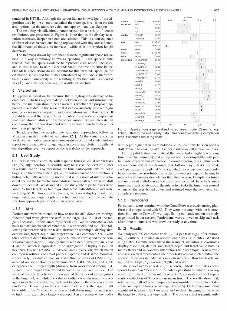
Fig. 5. Results from a generalized mixed linear model (Gamma, log-linked) fitted to the user study data. Response variable is completiontime. Estimates are in log scale.
with depth higher than 3 are hidden (i.e., t3) can only be seen upon adrill down. The crossing of all factors resulted in 288 interactive tasks.
During pilot testing, we realized that some tasks might take a longtime (over two minutes), and a long session is incompatible with par-ticipants’ expectations of fairness in crowdsourcing tasks. Thus, eachsession consisted of one training task followed by 8 tasks. In total,each participant completed 9 tasks, which were assigned randomlybased on display resolution, in order to avoid participants having tointeract with visualizations larger than their screen. Completion timesand number of drill-down interactions were recorded. In order to min-imize the effect of latency, in the interactive tasks the timer was pausedwhenever the user drilled down, and resumed once the new view wascompletely rendered.
5.1.2 ParticipantsParticipants were recruited with the CrowdFlower crowdsourcing plat-form and compensated with $2. They were presented with the instruc-tions both on the CrowdFlower page listing our study and on the studypage hosted in our servers. Participants were allowed to skip each taskafter three minutes and withdraw the study at any time.
5.1.3 ResultsWe analyzed 980 completed trials (∼ 3.4 per task avg.) after remov-ing 96 outliers. The median session length was 11 minutes. We useda log-linked Gamma generalized linear model, including as covariatesdisplay resolution, dataset size, target depth and target value both asmain effects and in two-way interactions with technique. A new vari-able was created representing the order tasks are completed within thesession. User was included as a random intercept. Baseline levels aret∞, 1920x1080px, top, average, depth and order 0.
The model intercept is 4.37 (79 seconds). Model estimates corre-spond to increase/decrease in the intercept estimate, which is in logscale. For instance, for an intercept of 4.37, a variation of -0.1 repre-sents a reduction of 8 seconds in mean time. The results show that,relative to t∞, all other techniques are responsible for a significant de-crease in response times on average (Figure 5). Order has a small, butsignificant negative effect on times and so does changing the value ofthe target to outlier, to a larger extent. The outlier effect is significantly
VERAS AND COLLINS: OPTIMIZING HIERARCHICAL VISUALIZATIONS WITH THE MINIMUM DESCRIPTION LENGTH PRINCIPLE 637
Fig. 4. Treemap visualizations generated with the display-tailored MDL procedure, with the following resolutions: 375x400px, 375x667px and1920x1080px. More abstract tree cuts are selected for smaller displays.
As in (12), we assume that P(l) is estimated by normalizing P(C)with respect to the leaves dominated by C:
P(l) =
{P(C)|C| if P(C)> 0
c if P(C) = 0(23)
where c is a constant representing the estimated probability of theleaves under a class whose rounded area is zero, and be thought of asan uninformed probability. We can set c to an arbitrarily small valueso as to penalize cuts featuring subpixel areas or, more sensibly, de-fine c as the sum of the probabilities of the “invisible” classes in a cut,divided by the total number of tree leaves under such classes. Thepiecewise function above can also be defined in a more conservativeway; for example, setting P(l) = c if A′(C) < δ , in order to penalizecuts with small areas, where δ is the smallest visible area. For exam-ple, a 3x3 pixel area on a high resolution wall-sized display.
The data description length is L(G | T ), the log of the followinglikelihood of G (as discussed in Section 2.1):
L (G | T ) = ∏l∈L
P(l)A(l) (24)
It is worth mentioning that the expression above is not strictly a like-lihood, but a power of the likelihood, since the data counts have beenmultiplied by a common factor that converts them to areas. Finally,the information criterion for selection of treemaps is:
L(T ,G) = L(T )+L(G | T ) = 2k log2 D− ∑C∈Γ
A(C) log2 P(l) (25)
4.2 SunburstThe structure of a sunburst can be thought of as a series of overlappingdisks, one for each tree level. A tree cut can be represented as a vectorof arcs Q. The central angle of the arc of a class equals the sum ofits children’s angles. Arc radius is proportional to the depth of a classin the tree: R j = ( j+1)∆R, with R j being the radius of all classes ofdepth j, and ∆R = D/2(h+1), where D is the sunburst diameter andh is the tree height.
It is reasonable to assume that users decode a sunburst by estimatingthe ratio of the arc length of a class and the circumference of the diskthat corresponds to the tree level where the class belongs. Assumingthe sunburst is sized to optimally fit the screen, as more levels are dis-played, the radius of each tree level’s disk is reduced, and estimatingthe value of a class becomes more difficult. This implies that selectingthe best tree cut depends on how many levels are displayed, and vice-versa. For example, a class with a relatively low frequency and depth
2, might be readable when displaying only three levels of a tree, butcan be rendered invisible when eight more levels are displayed, as thelevel disks will shrink.
Consequently, we need to run two rounds of minimization of thedescription length. In the first, we select the best tree cut under eachvalue of ∆R, restricting the levels of h; in the second, we select the bestof the tree cuts from the previous step. This is only valid if we definethe encoding of the data in a way that tree cut models are comparableacross values of ∆R; that is, they need to encode the same quantities.
We define the following mapping of S, where function A is the areaof the arc sector of radius D/2, which is independent of ∆R.
(A◦ f )(l) = A( f (l)) =f (l)|S|
π(D/2)2. (26)
A sunburst needs only two integers to inform each area, correspond-ing to the pixel indexes of the endpoints of an arc:
L(Q) = 2k log2 D. (27)
The arc length s of a class C at depth j is:
s(C) =f (C)
|S|2πR j. (28)
A′(C) is calculated analogously to (21), based on the rounded arclength:
A′(C) = �s(C)+1/2� (D/2)2
2R(C), (29)
which means that the decoded area of arcs with length smaller than .5is 0, due to the pixel resolution constraint. The estimated probabilityof a class is, thus:
P(C) =A′(C)
π(D/2)2 (30)
4.3 Proof-of-conceptTo illustrate the use of our display-tailored MDL procedure, we devel-oped two prototype visualizations (treemap and sunburst) of the Di-rectory Mozilla (DMOZ) dataset. As of November, 24, 2014, DMOZconsisted of 3,847,266 web pages, categorized under a total of 782,031topics. We selected the subtree under the prefix “Top/World”, whichcontains 2,083,282 pages written in English under 498,487 topics.We wrote browser-based clients that request tree cuts from a Node.jsserver. The parameters required by the server are display size androot node ID. The layouts are calculated in the server using D3 and
rendered in HTML. Although the server has no knowledge of the al-gorithm used by the client to calculate the treemap, it relies on the fairassumption that the areas are calculated approximately as Section 4.
The resulting visualizations, parametrized for a variety of screenresolutions, are presented in Figure 4. Note that as the display reso-lution increases, deeper tree cuts are selected. This is a consequenceof fewer classes in such cuts being represented with tiny areas; hence,the likelihood of these cuts increases, while their description lengthdecreases.
The treemaps drawn by our client allocate significant space for la-bels, in a way commonly known as “padding”. That space is sub-tracted from the space available to represent each node’s ancestors,and is also meant to help users understand the tree structure better.Our MDL calculations do not account for this “wasted” space (in theestimation sense) and the clutter introduced by the labels; therefore,there is more complexity in the resulting views than what is encodedin L(T ). We consider, however, the results satisfactory.
5 VALIDATION
This paper is based on the premise that a high-quality display of hi-erarchical data has a good balance between clutter and information;hence, the main question to be answered is whether the proposed ap-proach is scalable, in the sense that it can consistently produce high-quality views under varying display resolutions and dataset sizes. Itshould be noted that it is not our intention to provide a comprehen-sive evaluation of abstraction approaches; instead, we are interested incomparing the proposed method with reasonable baselines to put itsquality in perspective.
To address this, we adopted two validation approaches, followingMunzner’s nested model of validation [21]. At the visual encodinglevel, we test performance in a comparative controlled study, and wereport on a quantitative image analysis measuring clutter. Finally, atthe algorithm level, we report on the scalability of the approach.
5.1 User StudyClutter is shown to correlate with response times in visual search tasks[12, 25, 30]; therefore, a sensible way to assess the level of clutterin a visualization is by measuring the time participants take to locatetargets. In hierarchical displays, an important caveat of abstraction ishiding potentially interesting nodes; that is, if a node of interest is lo-cated deep in the hierarchy, more abstract views will require more drilldowns to locate it. We designed a user study where participants wereasked to find targets in treemaps abstracted with different methods,including MDL. Among other factors, we varied display resolution,target value, and target depth in the tree, and examined how each ab-straction approach performed in interactive tasks.
5.1.1 TasksParticipants were instructed on how to use the drill down (re-rooting)function and were given the path to the target (i.e., a list of the tar-get’s ancestors); for instance: Top/Arts/Music. We implemented a CSShack to make labels not searchable with a browser’s find tool. The fol-lowing factors varied in the tasks: abstraction technique, display size,dataset size, target depth, and target value. We compared MDL withthree levels of depth threshold: t3 and t4, which correspond to the con-servative approaches of capping nodes with depth greater than 3 and4, and t∞, which is equivalent to no aggregation. Display resolutionhas three levels: 375x667, 1024x768, and 1920x1080, which matchcommon resolutions of smart phones, laptops, and desktop monitors,respectively. For dataset size, we tested three subtrees of DMOZ: top,arts and soccer, containing approximately 500,000, 55,000, and 3,000categories each. Target depth (distance from root) varied among 3, 4,5, and 7; and target value varied between average and outlier. Thevalue of average targets was the average of the values of all categoriesin the target’s level, while the value of outliers was ten times the aver-age. Given these constraints, the target location in the tree was chosenrandomly. Depending on the combination of factors, the target mightbe visible in the “overview” screen or drill down might be necessaryto find it; for example, a target with depth 4 in a treemap where nodes
Fig. 5. Results from a generalized mixed linear model (Gamma, log-linked) fitted to the user study data. Response variable is completiontime. Estimates are in log scale.
with depth higher than 3 are hidden (i.e., t3) can only be seen upon adrill down. The crossing of all factors resulted in 288 interactive tasks.
During pilot testing, we realized that some tasks might take a longtime (over two minutes), and a long session is incompatible with par-ticipants’ expectations of fairness in crowdsourcing tasks. Thus, eachsession consisted of one training task followed by 8 tasks. In total,each participant completed 9 tasks, which were assigned randomlybased on display resolution, in order to avoid participants having tointeract with visualizations larger than their screen. Completion timesand number of drill-down interactions were recorded. In order to min-imize the effect of latency, in the interactive tasks the timer was pausedwhenever the user drilled down, and resumed once the new view wascompletely rendered.
5.1.2 ParticipantsParticipants were recruited with the CrowdFlower crowdsourcing plat-form and compensated with $2. They were presented with the instruc-tions both on the CrowdFlower page listing our study and on the studypage hosted in our servers. Participants were allowed to skip each taskafter three minutes and withdraw the study at any time.
5.1.3 ResultsWe analyzed 980 completed trials (∼ 3.4 per task avg.) after remov-ing 96 outliers. The median session length was 11 minutes. We useda log-linked Gamma generalized linear model, including as covariatesdisplay resolution, dataset size, target depth and target value both asmain effects and in two-way interactions with technique. A new vari-able was created representing the order tasks are completed within thesession. User was included as a random intercept. Baseline levels aret∞, 1920x1080px, top, average, depth and order 0.
The model intercept is 4.37 (79 seconds). Model estimates corre-spond to increase/decrease in the intercept estimate, which is in logscale. For instance, for an intercept of 4.37, a variation of -0.1 repre-sents a reduction of 8 seconds in mean time. The results show that,relative to t∞, all other techniques are responsible for a significant de-crease in response times on average (Figure 5). Order has a small, butsignificant negative effect on times and so does changing the value ofthe target to outlier, to a larger extent. The outlier effect is significantly
638 IEEE TRANSACTIONS ON VISUALIZATION AND COMPUTER GRAPHICS, VOL. 23, NO. 1, JANUARY 2017
Fig. 6. Number of drill-down interactions needed to complete a singletrial of the study, grouped by abstraction technique and target value.
and slightly larger for the MDL approach, although the differences inestimates are not dramatic. Interestingly, depth does not seem to sig-nificantly affect the response variable. This may be due to our notaccounting for the time for new views to load when drilling down. Adecrease in dataset size improves completion times only for t∞, and inthe smallest dataset condition (soccer), both t3 and t4 perform worsethan t∞. This is probably due to participants having to drill-down witht3 and t4, while the target is already visible with MDL and t∞. Thisexplains why the effect sizes are larger for soccer than for arts.
Figure 6 gives the distribution of the number of drill-down interac-tions needed to complete one trial, grouped by abstraction techniqueand target value. In the average target value condition, the distribu-tion of values for MDL is skewed to the right compared to all otherapproaches; that is, it required fewer drill downs. In the outlier condi-tion, MDL was better than t3 and t4, and similar to t∞.
5.1.4 DiscussionThe results confirm that lack of abstraction in views of large hierar-chies is detrimental to user performance, at least in visual search tasks.In that respect, even highly abstract approaches, such as t3 and t4, arebetter than unabstracted views. However, as we are not accountingfor the latency between drill downs, it is possible that in high latencyenvironments the benefits of abstraction are cancelled by the effect oflatency when locating targets requires drill down. In such a case, Fig-ure 6 suggests that MDL would require fewer drill-downs than t3 andt4. The fact that a reduction in dataset size was detrimental to userperformance in all abstraction conditions suggests that abstraction forsmall datasets is overkill; nevertheless, compared to t3 and t4, MDLhad the smallest increase in response time upon dataset reduction.
We expected outlier target to be easier to spot, as their size is tentimes larger than the average. The fact that MDL benefits the most ofthe outlier condition is likely a result of the MDL tendency to exposenodes with large model residuals.
Overall, the average response time of MDL was very similar to thatof depth threshold approaches, even though the average clutter in MDLviews tends to be higher. In the next section, we investigate the behav-ior of MDL views using an analytical measure of clutter.
5.2 Feature Congestion MeasureTo complement the analysis of the previous section, we compared thesame abstraction techniques with the feature congestion measure ofclutter [25], which is based on the notion that clutter in a display isassociated with degrading performance in visual search. It essentiallymeasures the difficulty of adding a new, salient item to a display. Themeasure computes the local variability of color and contrast luminanceat multiple scales, then combines the values over space and scale togenerate a scalar.
We generated treemap views of the DMOZ’s subtree “Top/World”,the same used throughout this paper, in resolutions ranging from100x100px to 2400x2400px, with the four abstraction approaches
4
6
8
10
12
0 500 1000 1500 2000 2500width
log(count)
0.09
0.12
0.15
0.18
0.21
0 500 1000 1500 2000 2500width
clutter
abstraction t∞ t3 t4 MDL
Fig. 7. Left: Level of clutter computed with the Feature Congestionmeasure as a function of display size. Right: Node count as a functionof display size. In both charts, dataset is DMOZ, and aspect ratio is 1:1.
tested in our user study: t∞, t3, t4, and MDL. We then calculatedthe featured congestion measure using only contrast luminance, as ourtreemaps do not vary color. In addition, the views were generatedwithout labels, in order to focus on clutter caused by tree structure.Padding is kept, as it is usually necessary for understanding structurein treemaps featuring deep levels.
The results of the experiment are shown in Figure 7, left. The clut-ter of t∞ views remains constant and high across the whole range ofresolutions. t3 and t4 decrease exponentially as the resolution grows.Just like t∞, the clutter in MDL views remains constant, but is lowerthan t∞. Note that for small displays, MDL ends up “falling back”to t3 and t4. As space becomes available, the distance between MDLand the depth thresholded views becomes higher, with MDL filling thespace with more data.
While clutter is often considered to be unwanted, it is positivelycorrelated with information density, and our approach attempts to finda balance. So, while the clutter of t3 and t4 drops dramatically at largescreen sizes, so does the information density. Clutter can be comparedwith the number of nodes visible in the visualizations as seen in Figure7, right. MDL, t3, and t4 consistently reveal far fewer nodes than t∞.The number of nodes revealed by MDL increases with screen size,while maintaining a roughly constant level of clutter. We argue thatwhile MDL reveals a smaller number of nodes at screen width 1024px,compared to t3, and the clutter is higher, this is due to the better (moreuniform) distribution of nodes across the space, as seen in Figure 8.
Woodruff et al. [31] argue in favor of constant information density(e.g., constant number of objects per area) across x, y and z dimen-sions of a multiscale visualization. They achieve that automaticallyby modifying the visual representation of data points and by adjustingthe level of abstraction unevenly. Figure 8 (middle) demonstrates thatMDL can also approximate constant information density across x andy dimensions. In addition, the results of the feature congestion exper-iment suggest that MDL approximates constant information densityacross display resolutions. Across the z dimension (drill-down) wesaw variations in the information density caused by the expansion ofnodes that have many children (fan out effect [4]). Unlike VIDA [31]and GrouseFlocks [4], which create new aggregates to minimize fanout, our method preserves the original hierarchy structure. As a result,if there are strong variations in how wide the first levels of subtreesare, the information density can vary.
5.3 Scalability AnalysisOur algorithm is a customization and application of the approach of Liand Abe, with the additional optimization step of including a factor ofdisplay size. They find that determining the MDL tree cut terminatesin time O(NxS), where N denotes the number of leaf nodes in the inputtree T and S denotes the input sample size. Our algorithm increasesthis procedure by the transformation from the data domain to the pixeldomain, and the estimation of the probabilities of leaves, both of whichare O(NxS). As S is generally much larger than N, our algorithmscales roughly linearly with the size of the dataset.
Any overhead encountered by generating a display-optimized treecut could be shifted to a server-side pre-calculation, for example, to
Fig. 8. Treemap views of the DMOZ dataset for a 1024x768px display. On the left, the full view of the dataset. In the middle, the level of detail isbased on the best MDL tree cut (uneven). On the right, an even cut is performed below level 4 of the tree. The MDL tree cuts yield a better balanceof information density and clutter.
Fig. 9. Subtle visual cues for collapsed nodes using texture (treemap)and border thickness (sunburst).
pre-cache the tree cut for a variety of standard screen sizes, therebyeliminating any delay incurred by the tree cut operation. The resultingtrees generally better balance information density with the number ofnodes, and will render faster and consume fewer client resources thanan equivalent full tree, and show a more uniform information densitythan a fixed-level tree cut.
6 DISCUSSION
Generality: With the formulae for treemap and sunburst visualiza-tions, we exemplified how model selection criteria can be written forvisualizations under the MDL framework. We believe that MDL canbe applied to many other kinds of hierarchical visualizations where(a) some visual aspect of the nodes is weighted by a score, and (b)the scores are cumulative. This might include visualizations thatare not traditionally hierarchical but were augmented with multiscalefunctionality, such as aggregated scatterplots, parallel coordinates andnode-link diagrams [11]. Defining criteria for new classes of visual-ization involves the specification of three main expressions:
1. The transformation from the data domain to the visualization do-main (pixel units) (A(C)).
2. Number of bits necessary to encode the visualization (L(V )).
3. How probabilities of tree leaves are estimated from the visualrepresentation of classes (P(l)).
Uniform distribution assumption: Behind the estimation of theprobability of leaves given a class is the assumption of uniform prob-ability. If this assumption is not reasonable in a certain applicationdomain, P(l) can be easily changed to reflect a different probabilitydistribution. A case where this might be useful is when depicting ge-ographic information, where the user might have a prior assumptionabout the distribution; for example, given a certain value for the Stateof New York (e.g., gross product), one might expect that value to beconcentrated in New York City. In many other cases, lacking priorknowledge, we expect the uniform distribution to be fairly reasonable.
An important limitation is that if the data is uniformly distributed,the tree cut generated will be the most abstract possible (i.e. the root).This occurs, for example, if the value of every leaf is 1. Likewise, ifa different distribution is used and the data conforms exactly, the treecut will be overgeneralized.
Interpretation: It is especially important in models such as ours,where abstraction is calculated algorithmically, that the presence ofdata abstraction is made apparent, in ways that are not distracting tothe main task of working with a visualization. While our techniqueand evaluation focus on the level of abstraction, we have begun an in-vestigation into the representation problem. Figure 9 suggests prelim-inary visual designs which subtly distinguish aggregates from regularleaves. On treemaps, aggregates are textured; on sunbursts, collapsednodes are decorated with a colored, thicker border.
7 CONCLUSION
In this paper we have presented a technique for using the MDL Prin-ciple, extended with considerations of display space, in order to createoptimized views of hierarchical datasets which fit the “analyze first,show the important” first step of the visual analytics pipeline. In ad-dition to providing overviews customized to dataset and display sizecharacteristics, the display-optimized tree cuts can be interactively ex-panded by changing the weighting parameters.
The number of nodes displayed in a display-optimized MDL treecut is similar to those in an even tree cut at a set depth, but fewer thanshowing a full tree. This increases the rendering efficiency, resultingin a performance gain in web-based visualization applications, whereprocessing resources, memory, and display space may be constrained(e.g. on mobile devices). In addition, on small screens and any touchdevice where rendered elements are small, interaction accuracy canbe difficult due to the “fat fingers” problem. Our technique appliesabstraction in cluttered areas of a visualization, which will likely im-prove target selection accuracy.
We have demonstrated our technique applied to two datasets acrosstwo different hierarchical visualization types, treemap and sunburstdiagrams, and outlined the steps required to generalize the approachto other visualization types. Display-optimized MDL tree cuts mayprove especially useful due to their general nature — they are not cus-tomized to dataset characteristics. However, it is also possible to tailorthem to the dataset, for example, by basing the tree cut on a selecteddata attribute, as long as that attribute is quantitative on the leaves andcumulative in the hierarchy.
In the future, we plan to apply the display-optimized MDL treecut to new visualization types. In addition, we see promise in thechallenge of developing new methods for representing abstraction. Fi-nally, while we demonstrate the possibilities of interactive drill downto deeper levels of the tree cut using a fixed step size, we plan to inves-tigate ways to automatically tailor the drill down step based on datasetcharacteristics, display space, and to harmonize tree cut drill downwith more traditional techniques to click and open branches manually.
VERAS AND COLLINS: OPTIMIZING HIERARCHICAL VISUALIZATIONS WITH THE MINIMUM DESCRIPTION LENGTH PRINCIPLE 639
Fig. 6. Number of drill-down interactions needed to complete a singletrial of the study, grouped by abstraction technique and target value.
and slightly larger for the MDL approach, although the differences inestimates are not dramatic. Interestingly, depth does not seem to sig-nificantly affect the response variable. This may be due to our notaccounting for the time for new views to load when drilling down. Adecrease in dataset size improves completion times only for t∞, and inthe smallest dataset condition (soccer), both t3 and t4 perform worsethan t∞. This is probably due to participants having to drill-down witht3 and t4, while the target is already visible with MDL and t∞. Thisexplains why the effect sizes are larger for soccer than for arts.
Figure 6 gives the distribution of the number of drill-down interac-tions needed to complete one trial, grouped by abstraction techniqueand target value. In the average target value condition, the distribu-tion of values for MDL is skewed to the right compared to all otherapproaches; that is, it required fewer drill downs. In the outlier condi-tion, MDL was better than t3 and t4, and similar to t∞.
5.1.4 DiscussionThe results confirm that lack of abstraction in views of large hierar-chies is detrimental to user performance, at least in visual search tasks.In that respect, even highly abstract approaches, such as t3 and t4, arebetter than unabstracted views. However, as we are not accountingfor the latency between drill downs, it is possible that in high latencyenvironments the benefits of abstraction are cancelled by the effect oflatency when locating targets requires drill down. In such a case, Fig-ure 6 suggests that MDL would require fewer drill-downs than t3 andt4. The fact that a reduction in dataset size was detrimental to userperformance in all abstraction conditions suggests that abstraction forsmall datasets is overkill; nevertheless, compared to t3 and t4, MDLhad the smallest increase in response time upon dataset reduction.
We expected outlier target to be easier to spot, as their size is tentimes larger than the average. The fact that MDL benefits the most ofthe outlier condition is likely a result of the MDL tendency to exposenodes with large model residuals.
Overall, the average response time of MDL was very similar to thatof depth threshold approaches, even though the average clutter in MDLviews tends to be higher. In the next section, we investigate the behav-ior of MDL views using an analytical measure of clutter.
5.2 Feature Congestion MeasureTo complement the analysis of the previous section, we compared thesame abstraction techniques with the feature congestion measure ofclutter [25], which is based on the notion that clutter in a display isassociated with degrading performance in visual search. It essentiallymeasures the difficulty of adding a new, salient item to a display. Themeasure computes the local variability of color and contrast luminanceat multiple scales, then combines the values over space and scale togenerate a scalar.
We generated treemap views of the DMOZ’s subtree “Top/World”,the same used throughout this paper, in resolutions ranging from100x100px to 2400x2400px, with the four abstraction approaches
4
6
8
10
12
0 500 1000 1500 2000 2500width
log(count)
0.09
0.12
0.15
0.18
0.21
0 500 1000 1500 2000 2500width
clutter
abstraction t∞ t3 t4 MDL
Fig. 7. Left: Level of clutter computed with the Feature Congestionmeasure as a function of display size. Right: Node count as a functionof display size. In both charts, dataset is DMOZ, and aspect ratio is 1:1.
tested in our user study: t∞, t3, t4, and MDL. We then calculatedthe featured congestion measure using only contrast luminance, as ourtreemaps do not vary color. In addition, the views were generatedwithout labels, in order to focus on clutter caused by tree structure.Padding is kept, as it is usually necessary for understanding structurein treemaps featuring deep levels.
The results of the experiment are shown in Figure 7, left. The clut-ter of t∞ views remains constant and high across the whole range ofresolutions. t3 and t4 decrease exponentially as the resolution grows.Just like t∞, the clutter in MDL views remains constant, but is lowerthan t∞. Note that for small displays, MDL ends up “falling back”to t3 and t4. As space becomes available, the distance between MDLand the depth thresholded views becomes higher, with MDL filling thespace with more data.
While clutter is often considered to be unwanted, it is positivelycorrelated with information density, and our approach attempts to finda balance. So, while the clutter of t3 and t4 drops dramatically at largescreen sizes, so does the information density. Clutter can be comparedwith the number of nodes visible in the visualizations as seen in Figure7, right. MDL, t3, and t4 consistently reveal far fewer nodes than t∞.The number of nodes revealed by MDL increases with screen size,while maintaining a roughly constant level of clutter. We argue thatwhile MDL reveals a smaller number of nodes at screen width 1024px,compared to t3, and the clutter is higher, this is due to the better (moreuniform) distribution of nodes across the space, as seen in Figure 8.
Woodruff et al. [31] argue in favor of constant information density(e.g., constant number of objects per area) across x, y and z dimen-sions of a multiscale visualization. They achieve that automaticallyby modifying the visual representation of data points and by adjustingthe level of abstraction unevenly. Figure 8 (middle) demonstrates thatMDL can also approximate constant information density across x andy dimensions. In addition, the results of the feature congestion exper-iment suggest that MDL approximates constant information densityacross display resolutions. Across the z dimension (drill-down) wesaw variations in the information density caused by the expansion ofnodes that have many children (fan out effect [4]). Unlike VIDA [31]and GrouseFlocks [4], which create new aggregates to minimize fanout, our method preserves the original hierarchy structure. As a result,if there are strong variations in how wide the first levels of subtreesare, the information density can vary.
5.3 Scalability AnalysisOur algorithm is a customization and application of the approach of Liand Abe, with the additional optimization step of including a factor ofdisplay size. They find that determining the MDL tree cut terminatesin time O(NxS), where N denotes the number of leaf nodes in the inputtree T and S denotes the input sample size. Our algorithm increasesthis procedure by the transformation from the data domain to the pixeldomain, and the estimation of the probabilities of leaves, both of whichare O(NxS). As S is generally much larger than N, our algorithmscales roughly linearly with the size of the dataset.
Any overhead encountered by generating a display-optimized treecut could be shifted to a server-side pre-calculation, for example, to
Fig. 8. Treemap views of the DMOZ dataset for a 1024x768px display. On the left, the full view of the dataset. In the middle, the level of detail isbased on the best MDL tree cut (uneven). On the right, an even cut is performed below level 4 of the tree. The MDL tree cuts yield a better balanceof information density and clutter.
Fig. 9. Subtle visual cues for collapsed nodes using texture (treemap)and border thickness (sunburst).
pre-cache the tree cut for a variety of standard screen sizes, therebyeliminating any delay incurred by the tree cut operation. The resultingtrees generally better balance information density with the number ofnodes, and will render faster and consume fewer client resources thanan equivalent full tree, and show a more uniform information densitythan a fixed-level tree cut.
6 DISCUSSION
Generality: With the formulae for treemap and sunburst visualiza-tions, we exemplified how model selection criteria can be written forvisualizations under the MDL framework. We believe that MDL canbe applied to many other kinds of hierarchical visualizations where(a) some visual aspect of the nodes is weighted by a score, and (b)the scores are cumulative. This might include visualizations thatare not traditionally hierarchical but were augmented with multiscalefunctionality, such as aggregated scatterplots, parallel coordinates andnode-link diagrams [11]. Defining criteria for new classes of visual-ization involves the specification of three main expressions:
1. The transformation from the data domain to the visualization do-main (pixel units) (A(C)).
2. Number of bits necessary to encode the visualization (L(V )).
3. How probabilities of tree leaves are estimated from the visualrepresentation of classes (P(l)).
Uniform distribution assumption: Behind the estimation of theprobability of leaves given a class is the assumption of uniform prob-ability. If this assumption is not reasonable in a certain applicationdomain, P(l) can be easily changed to reflect a different probabilitydistribution. A case where this might be useful is when depicting ge-ographic information, where the user might have a prior assumptionabout the distribution; for example, given a certain value for the Stateof New York (e.g., gross product), one might expect that value to beconcentrated in New York City. In many other cases, lacking priorknowledge, we expect the uniform distribution to be fairly reasonable.
An important limitation is that if the data is uniformly distributed,the tree cut generated will be the most abstract possible (i.e. the root).This occurs, for example, if the value of every leaf is 1. Likewise, ifa different distribution is used and the data conforms exactly, the treecut will be overgeneralized.
Interpretation: It is especially important in models such as ours,where abstraction is calculated algorithmically, that the presence ofdata abstraction is made apparent, in ways that are not distracting tothe main task of working with a visualization. While our techniqueand evaluation focus on the level of abstraction, we have begun an in-vestigation into the representation problem. Figure 9 suggests prelim-inary visual designs which subtly distinguish aggregates from regularleaves. On treemaps, aggregates are textured; on sunbursts, collapsednodes are decorated with a colored, thicker border.
7 CONCLUSION
In this paper we have presented a technique for using the MDL Prin-ciple, extended with considerations of display space, in order to createoptimized views of hierarchical datasets which fit the “analyze first,show the important” first step of the visual analytics pipeline. In ad-dition to providing overviews customized to dataset and display sizecharacteristics, the display-optimized tree cuts can be interactively ex-panded by changing the weighting parameters.
The number of nodes displayed in a display-optimized MDL treecut is similar to those in an even tree cut at a set depth, but fewer thanshowing a full tree. This increases the rendering efficiency, resultingin a performance gain in web-based visualization applications, whereprocessing resources, memory, and display space may be constrained(e.g. on mobile devices). In addition, on small screens and any touchdevice where rendered elements are small, interaction accuracy canbe difficult due to the “fat fingers” problem. Our technique appliesabstraction in cluttered areas of a visualization, which will likely im-prove target selection accuracy.
We have demonstrated our technique applied to two datasets acrosstwo different hierarchical visualization types, treemap and sunburstdiagrams, and outlined the steps required to generalize the approachto other visualization types. Display-optimized MDL tree cuts mayprove especially useful due to their general nature — they are not cus-tomized to dataset characteristics. However, it is also possible to tailorthem to the dataset, for example, by basing the tree cut on a selecteddata attribute, as long as that attribute is quantitative on the leaves andcumulative in the hierarchy.
In the future, we plan to apply the display-optimized MDL treecut to new visualization types. In addition, we see promise in thechallenge of developing new methods for representing abstraction. Fi-nally, while we demonstrate the possibilities of interactive drill downto deeper levels of the tree cut using a fixed step size, we plan to inves-tigate ways to automatically tailor the drill down step based on datasetcharacteristics, display space, and to harmonize tree cut drill downwith more traditional techniques to click and open branches manually.
640 IEEE TRANSACTIONS ON VISUALIZATION AND COMPUTER GRAPHICS, VOL. 23, NO. 1, JANUARY 2017
REFERENCES
[1] J. Abello, F. Van Ham, and N. Krishnan. ASK-GraphView: Alarge scale graph visualization system. IEEE Trans. on Visual-ization and Computer Graphics, 12(5):669–676, 2006.
[2] N. Andrienko and G. Andrienko. Spatial generalisation and ag-gregation of massive movement data. IEEE Trans. on Visualiza-tion and, 17(2):205–19, 2010.
[3] D. Archambault and D. Greene. ThemeCrowds: Multiresolutionsummaries of twitter usage. International Workshop on Searchand Mining User-generated Contents, pages 77–84, 2011.
[4] D. Archambault, T. Munzner, and D. Auber. GrouseFlocks:Steerable exploration of graph hierarchy space. IEEE Trans. onVisualization and Computer Graphics, 14(4):900–913, 2008.
[5] S. Baldassi, N. Megna, and D. C. Burr. Visual Clutter CausesHigh-Magnitude Errors. PLoS Biology, 4(3):e56, 2006.
[6] A. Brew, D. Greene, D. Archambault, and P. Cunningham. De-riving insights from national happiness indices. Proceedings -IEEE International Conference on Data Mining, ICDM, pages53–60, 2011.
[7] M. Chuah. Dynamic aggregation with circular visual designs.In Proceedings IEEE Symposium on Information Visualization,pages 1–9, 1998.
[8] C. Collins, S. Carpendale, and G. Penn. DocuBurst: Visualizingdocument content using language structure. Computer GraphicsForum, 28(3):1039–1046, jun 2009.
[9] Q. Cui, M. Ward, E. Rundensteiner, and J. Yang. Measuringdata abstraction quality in multiresolution visualizations. IEEETrans. on Visualization and Computer Graphics, 12(5):709–716,2006.
[10] G. Ellis and A. Dix. A taxonomy of clutter reduction for informa-tion visualisation. IEEE Trans. on Visualization and ComputerGraphics, 13(6):1216–1223, 2007.
[11] N. Elmqvist and J.-D. Fekete. Hierarchical aggregation for infor-mation visualization: overview, techniques, and design guide-lines. IEEE Trans. on Visualization and Computer Graphics,16(3):439–54, 2010.
[12] S. Haroz and D. Whitney. How Capacity Limits of Attention In-fluence Information Visualization Effectiveness. IEEE Trans. onVisualization and Computer Graphics, 18(12):2402–2410, dec2012.
[13] D. Keim, F. Mansmann, J. Schneidewind, and H. Ziegler. Chal-lenges in Visual Data Analysis. In Proc. of the Int. Conv. onInformation Visualisation, pages 9–16. IEEE, 2006.
[14] D. Koutra, U. Kang, J. Vreeken, and C. Faloutsos. Summarizingand Understanding Large Graphs. Statistical Analysis and DataMining, 8(3):183–202, 2015.
[15] R. Lamarche-perrin, Y. Demazeau, and J.-m. Vincent. BuildingOptimal Macroscopic Representations of Complex Multi-agentSystems. In N.-T. Nguyen, R. Kowalczyk, J. Corchado, andJ. Bajo, editors, Trans. on Computational Collective IntelligenceXV, volume 8670, pages 1–27. Springer Berlin Heidelberg, 2014.
[16] R. Lamarche-perrin, L. M. Shnorr, J.-m. Vincent, and Y. De-mazeau. Evaluating Trace Aggregation Through Entropy Mea-sures for Optimal Performance Visualization of Large Dis-tributed Systems. Technical report, INRIA, 2012.
[17] T. C. M. Lee. A Minimum Description Length Based ImageSegmentation Procedure , and Its Comparison with a Cross-Validation-Based Segmentation Procedure. Journal of the Amer-ican Statistical Association, 95(1995):259–270, 1999.
[18] T. C. M. Lee. An Introduction to Coding Theory and the Two-Part Minimum Description Length Principle. International Sta-tistical Review, 69(2):169–183, 2001.
[19] H. Li and N. Abe. Generalizing Case Frames Using a Thesaurusand the MDL Principle. Computational linguistics, 24(2):217–244, 1998.
[20] G. a. Miller. The magical number seven, plus or minus two: somelimits on our capacity for processing information. Psychologicalreview, 101(2):343–352, 1956.
[21] T. Munzner. Visualization Analysis & Design. CRC Press, 2014.
[22] J. R. Quinlan and R. Rivest. Inferring Decision Trees Using theMinimum Description Length Principle. Information and Com-putation, 80(1989):227–248, 1989.
[23] J. Rissanen. A universal prior for integers and estimation byminimum description length. Annals of Statistics, 11(2):416–431, 1983.
[24] J. Rissanen. Stochastic Complexity in Statistical Inquiry. WorldScientific Publishing Co., Inc., River Edge, NJ, USA, 1989.
[25] R. Rosenholtz, Y. Li, Z. Jin, and J. Mansfield. Feature conges-tion: A measure of visual clutter. Journal of Vision, 6(6):827–827, 2010.
[26] R. Rosenholtz, Y. Li, and L. Nakano. Measuring visual clutter.Journal of vision, 7(2):17.1–22, 2007.
[27] B. Shneiderman. The eyes have it: a task by data type taxonomyfor information visualizations. In Proc. 1996 IEEE Symposiumon Visual Languages, pages 336–343. IEEE Comput. Soc. Press,1996.
[28] F. Topfer and W. Pillewizer. The Principles of Selection. TheCartographic Journal, 3(1):10–16, 1966.
[29] A. Wagner. Enriching a lexical semantic net with selectionalpreferences by means of statistical corpus analysis. In Pro-ceedings of the European Conference on Artificial Intelligence- ECAI, 2000.
[30] J. M. Wolfe. Visual Search. Attention, pages 1–41, 1998.
[31] A. Woodruff, J. Landay, and M. Stonebraker. Constant densityvisualizations of non-uniform distributions of data. In Proceed-ings of the 11th annual ACM symposium on User interface soft-ware and technology - UIST ’98, pages 19–28, 1998.
[32] Y. Wu, X. Liu, S. Liu, and K. L. Ma. ViSizer: A visualizationresizing framework. IEEE Trans. on Visualization and ComputerGraphics, 19(2):278–290, 2013.
[33] B. Yost and C. North. The perceptual scalability of visualiza-tion. IEEE Trans. on Visualization and Computer Graphics,12(5):837–844, 2006.