Optimizing Process Economic Performance Using Model Predictive Control James B. Rawlings and Rishi Amrit Department of Chemical and Biological Engineering University of Wisconsin–Madison International Workshop on Assessment and Future Directions of NMPC Pavia, Italy September 5, 2008 Rawlings and Amrit (UW) Economic MPC NMPC 2008 1 / 49
Transcript
Optimizing Process Economic Performance Using ModelPredictive Control
James B. Rawlings and Rishi Amrit
Department of Chemical and Biological EngineeringUniversity of Wisconsin–Madison
International Workshop on Assessment and Future Directions ofNMPC
The goal of optimal process operations is to maximize profit.— Helbig, Abel, and Marquardt (1998) . . . (−10 years)
Thus with more powerful capabilities, the determination ofsteady-state setpoints may simply become an unnecessaryintermediate calculation. Instead nonlinear, dynamic referencemodels could be used directly to optimize a profit objective.— Biegler and Rawlings (1991) . . . (−20 years)
In attempting to synthesize a feedback optimizing controlstructure, our main objective is to translate the economicobjective into process control objectives.— Morari, Arkun, and Stephanopoulos (1980) . . . (−30 years)
The goal of optimal process operations is to maximize profit.— Helbig, Abel, and Marquardt (1998)
. . . (−10 years)
Thus with more powerful capabilities, the determination ofsteady-state setpoints may simply become an unnecessaryintermediate calculation. Instead nonlinear, dynamic referencemodels could be used directly to optimize a profit objective.— Biegler and Rawlings (1991) . . . (−20 years)
In attempting to synthesize a feedback optimizing controlstructure, our main objective is to translate the economicobjective into process control objectives.— Morari, Arkun, and Stephanopoulos (1980) . . . (−30 years)
The goal of optimal process operations is to maximize profit.— Helbig, Abel, and Marquardt (1998) . . . (−10 years)
Thus with more powerful capabilities, the determination ofsteady-state setpoints may simply become an unnecessaryintermediate calculation. Instead nonlinear, dynamic referencemodels could be used directly to optimize a profit objective.— Biegler and Rawlings (1991) . . . (−20 years)
In attempting to synthesize a feedback optimizing controlstructure, our main objective is to translate the economicobjective into process control objectives.— Morari, Arkun, and Stephanopoulos (1980) . . . (−30 years)
The goal of optimal process operations is to maximize profit.— Helbig, Abel, and Marquardt (1998) . . . (−10 years)
Thus with more powerful capabilities, the determination ofsteady-state setpoints may simply become an unnecessaryintermediate calculation.
Instead nonlinear, dynamic referencemodels could be used directly to optimize a profit objective.— Biegler and Rawlings (1991) . . . (−20 years)
In attempting to synthesize a feedback optimizing controlstructure, our main objective is to translate the economicobjective into process control objectives.— Morari, Arkun, and Stephanopoulos (1980) . . . (−30 years)
The goal of optimal process operations is to maximize profit.— Helbig, Abel, and Marquardt (1998) . . . (−10 years)
Thus with more powerful capabilities, the determination ofsteady-state setpoints may simply become an unnecessaryintermediate calculation. Instead nonlinear, dynamic referencemodels could be used directly to optimize a profit objective.
— Biegler and Rawlings (1991) . . . (−20 years)
In attempting to synthesize a feedback optimizing controlstructure, our main objective is to translate the economicobjective into process control objectives.— Morari, Arkun, and Stephanopoulos (1980) . . . (−30 years)
The goal of optimal process operations is to maximize profit.— Helbig, Abel, and Marquardt (1998) . . . (−10 years)
Thus with more powerful capabilities, the determination ofsteady-state setpoints may simply become an unnecessaryintermediate calculation. Instead nonlinear, dynamic referencemodels could be used directly to optimize a profit objective.— Biegler and Rawlings (1991)
. . . (−20 years)
In attempting to synthesize a feedback optimizing controlstructure, our main objective is to translate the economicobjective into process control objectives.— Morari, Arkun, and Stephanopoulos (1980) . . . (−30 years)
The goal of optimal process operations is to maximize profit.— Helbig, Abel, and Marquardt (1998) . . . (−10 years)
Thus with more powerful capabilities, the determination ofsteady-state setpoints may simply become an unnecessaryintermediate calculation. Instead nonlinear, dynamic referencemodels could be used directly to optimize a profit objective.— Biegler and Rawlings (1991) . . . (−20 years)
In attempting to synthesize a feedback optimizing controlstructure, our main objective is to translate the economicobjective into process control objectives.— Morari, Arkun, and Stephanopoulos (1980) . . . (−30 years)
The goal of optimal process operations is to maximize profit.— Helbig, Abel, and Marquardt (1998) . . . (−10 years)
Thus with more powerful capabilities, the determination ofsteady-state setpoints may simply become an unnecessaryintermediate calculation. Instead nonlinear, dynamic referencemodels could be used directly to optimize a profit objective.— Biegler and Rawlings (1991) . . . (−20 years)
In attempting to synthesize a feedback optimizing controlstructure, our main objective is to translate the economicobjective into process control objectives.
The goal of optimal process operations is to maximize profit.— Helbig, Abel, and Marquardt (1998) . . . (−10 years)
Thus with more powerful capabilities, the determination ofsteady-state setpoints may simply become an unnecessaryintermediate calculation. Instead nonlinear, dynamic referencemodels could be used directly to optimize a profit objective.— Biegler and Rawlings (1991) . . . (−20 years)
In attempting to synthesize a feedback optimizing controlstructure, our main objective is to translate the economicobjective into process control objectives.— Morari, Arkun, and Stephanopoulos (1980)
The goal of optimal process operations is to maximize profit.— Helbig, Abel, and Marquardt (1998) . . . (−10 years)
Thus with more powerful capabilities, the determination ofsteady-state setpoints may simply become an unnecessaryintermediate calculation. Instead nonlinear, dynamic referencemodels could be used directly to optimize a profit objective.— Biegler and Rawlings (1991) . . . (−20 years)
In attempting to synthesize a feedback optimizing controlstructure, our main objective is to translate the economicobjective into process control objectives.— Morari, Arkun, and Stephanopoulos (1980) . . . (−30 years)
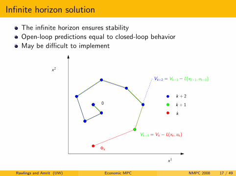
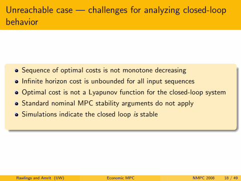
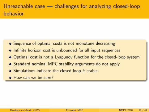
Theorem (Asymptotic Stability of Terminal Constraint MPC)
The optimal steady state is the asymptotically stable solution of theclosed-loop system under terminal constraint MPC. Its region of attractionis the steerable set.
(Rawlings, Bonne, Jørgensen, Venkat, and Jørgensen, 2008)
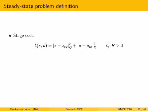
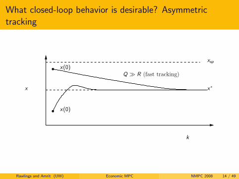
Stage cost:eco–MPC: L(x , u) = any strictly convex function
Cost function: V =N−1∑j=0
L(x(j), u(j))
Optimization: minu
V (u, x(0))
subject to:x+ = Ax + Bu u = {u(0), u(1), . . . u(N − 1)} u ∈ UControl law: u0(x) = u0(0, x)
Asymptotic stability: (x(k), u(k)) −→ (xe , ue), the optimal economicsteady state for the chosen L(x , u).Requires terminal constraint, terminal controller, or infinite horizon.
Stage cost:eco–MPC: L(x , u) = any strictly convex function
Cost function: V =N−1∑j=0
L(x(j), u(j))
Optimization: minu
V (u, x(0))
subject to:x+ = Ax + Bu u = {u(0), u(1), . . . u(N − 1)} u ∈ U
Control law: u0(x) = u0(0, x)
Asymptotic stability: (x(k), u(k)) −→ (xe , ue), the optimal economicsteady state for the chosen L(x , u).Requires terminal constraint, terminal controller, or infinite horizon.
Stage cost:eco–MPC: L(x , u) = any strictly convex function
Cost function: V =N−1∑j=0
L(x(j), u(j))
Optimization: minu
V (u, x(0))
subject to:x+ = Ax + Bu u = {u(0), u(1), . . . u(N − 1)} u ∈ UControl law: u0(x) = u0(0, x)
Asymptotic stability: (x(k), u(k)) −→ (xe , ue), the optimal economicsteady state for the chosen L(x , u).Requires terminal constraint, terminal controller, or infinite horizon.
Stage cost:eco–MPC: L(x , u) = any strictly convex function
Cost function: V =N−1∑j=0
L(x(j), u(j))
Optimization: minu
V (u, x(0))
subject to:x+ = Ax + Bu u = {u(0), u(1), . . . u(N − 1)} u ∈ UControl law: u0(x) = u0(0, x)
Asymptotic stability: (x(k), u(k)) −→ (xe , ue), the optimal economicsteady state for the chosen L(x , u).Requires terminal constraint, terminal controller, or infinite horizon.
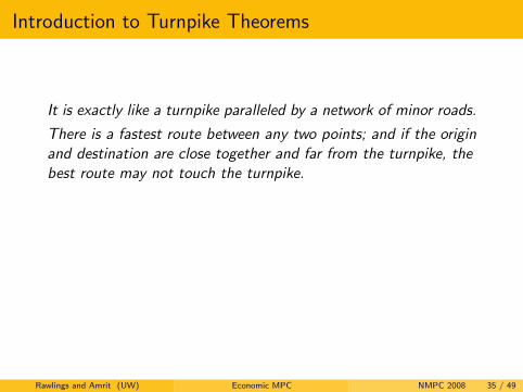
It is exactly like a turnpike paralleled by a network of minor roads.
There is a fastest route between any two points; and if the originand destination are close together and far from the turnpike, thebest route may not touch the turnpike.
But if the origin and destination are far enough apart, it willalways pay to get on the turnpike and cover distance at the bestrate of travel, even if this means adding a little mileage at eitherend.
I Consistent model for optimizing performanceI Consistent statement of process objectivesI Optimization software well developedI Linear dynamics and convex objectives well supportedI Leverage from industrial implementation of linear MPCI This is a big opportunity!
OpportunitiesI Performance advantageI Consistent model for optimizing performance
I Consistent statement of process objectivesI Optimization software well developedI Linear dynamics and convex objectives well supportedI Leverage from industrial implementation of linear MPCI This is a big opportunity!
OpportunitiesI Performance advantageI Consistent model for optimizing performanceI Consistent statement of process objectives
I Optimization software well developedI Linear dynamics and convex objectives well supportedI Leverage from industrial implementation of linear MPCI This is a big opportunity!
OpportunitiesI Performance advantageI Consistent model for optimizing performanceI Consistent statement of process objectivesI Optimization software well developed
I Linear dynamics and convex objectives well supportedI Leverage from industrial implementation of linear MPCI This is a big opportunity!
OpportunitiesI Performance advantageI Consistent model for optimizing performanceI Consistent statement of process objectivesI Optimization software well developedI Linear dynamics and convex objectives well supported
I Leverage from industrial implementation of linear MPCI This is a big opportunity!
OpportunitiesI Performance advantageI Consistent model for optimizing performanceI Consistent statement of process objectivesI Optimization software well developedI Linear dynamics and convex objectives well supportedI Leverage from industrial implementation of linear MPC
OpportunitiesI Performance advantageI Consistent model for optimizing performanceI Consistent statement of process objectivesI Optimization software well developedI Linear dynamics and convex objectives well supportedI Leverage from industrial implementation of linear MPCI This is a big opportunity!
E. M. B. Aske, S. Strand, and S. Skogestad. Coordinator MPC for maximizing plantthroughput. Comput. Chem. Eng., 32:195–204, 2008.
T. Backx, O. Bosgra, and W. Marquardt. Integration of model predictive control andoptimization of processes. In Advanced Control of Chemical Processes, June 2000.
L. T. Biegler and J. B. Rawlings. Optimization approaches to nonlinear model predictivecontrol. In Y. Arkun and W. H. Ray, editors, Chemical Process Control–CPCIV,pages 543–571. CACHE, 1991.
D. A. Carlson, A. B. Haurie, and A. Leizarowitz. Infinite Horizon Optimal Control.Springer Verlag, second edition, 1991.
D. DeHaan and M. Guay. Extremum seeking control of nonlinear systems withparametric uncertainties and state constraints. In Proceedings of the 2004 AmericanControl Conference, pages 596–601, July 2004.
R. Dorfman, P. Samuelson, and R. Solow. Linear Programming and Economic Analysis.McGraw-Hill, New York, 1958.
S. Engell. Feedback control for optimal process operation. J. Proc. Cont., 17:203–219,2007.
M. Guay and T. Zhang. Adaptive extremum seeking control of nonlinear dynamicsystems with parametric uncertainty. Automatica, 39:1283–1293, 2003.
M. Guay, D. Dochain, and M. Perrier. Adaptive extremum seeking control ofnonisothermal continuous stirred tank reactors with temperature constraints. InProceedings of the 42nd IEEE Conference on Decision and Control, Maui, Hawaii,December 2003.
A. Helbig, O. Abel, and W. Marquardt. Structural concepts for optimization basedcontrol of transient processes. In International Symposium on Nonlinear ModelPredictive Control, Ascona, Switzerland, 1998.
J. L. W. V. Jensen. Sur les fonctions convexes et les inegalites entre les valeursmoyennes. Acta Math., 30:175–193, 1906.
M. Krstic and H.-H. Wang. Stability of extremum seeking feedback for general nonlineardynamic systems. Automatica, 36:595–601, 2000.
M. Morari, Y. Arkun, and G. Stephanopoulos. Studies in the synthesis of controlstructures for chemical processes. Part I: Formulation of the problem. processdecomposition and the classification of the control tasks. Analysis of the optimizingcontrol structures. AIChE J., 26(2):220–232, 1980.
J. B. Rawlings, D. Bonne, J. B. Jørgensen, A. N. Venkat, and S. B. Jørgensen.Unreachable setpoints in model predictive control. Accepted for publication in IEEETAC, April 2008.
O. Rotava and A. Zanin. Multivariable control and real-time optimization — anindustrial practical view. Hydrocarbon Processing, pages 61–71, June 2005.
S. Skogestad. Plantwide control: the search for the self-optimizing control structure. J.Proc. Cont., 10:487–507, 2000.
A. C. Zanin, M. Tvrzska de Gouvea, and D. Odloak. Integrating real-time optimizationinto the model predictive controller of the FCC system. Control Eng. Practice, 10:819–831, 2002.
V. M. Zavala and L. T. Biegler. The advanced step nmpc controller: optimality, stabilityand robustness. To appear in Automatica, 2008.