Optimizing Providers’ Profit in Peer Networks Applying Automatic Pricing and Game Theory by Sohel Q. Khan B.S.E.E., The University of Kansas, USA, 1995 M.S.E.E., The University of Kansas, USA, 1998 Presented to the Department of Electrical Engineering and Computer Science and the Faculty of the Graduate School of the University of Kansas in partial fulfillment of the requirements for the degree of Doctor of Philosophy Committee: ________________________________ Prof. David W. Petr, Chair ________________________________ Prof. Victor Frost ________________________________ Prof. John Gauch ________________________________ Prof. Tyrone Duncan ________________________________ Prof. Bozenna Pasik-Duncan ________________________________ Prof. Jianbo Zhang The University of Kansas October 24, 2005
Transcript
Optimizing Providers’ Profit in Peer Networks Applying Automatic
Pricing and Game Theory
by
Sohel Q. Khan B.S.E.E., The University of Kansas, USA, 1995 M.S.E.E., The University of Kansas, USA, 1998
Presented to the Department of Electrical Engineering and Computer Science
and the Faculty of the Graduate School of the University of Kansas in partial fulfillment of the requirements for the degree of
Doctor of Philosophy
Committee: ________________________________ Prof. David W. Petr, Chair ________________________________ Prof. Victor Frost ________________________________ Prof. John Gauch ________________________________
Prof. Tyrone Duncan
________________________________ Prof. Bozenna Pasik-Duncan ________________________________ Prof. Jianbo Zhang
The University of Kansas October 24, 2005
2
The Dissertation Committee for Sohel Q. Khan certifies that this is the approved version of the following dissertation:
Optimizing Providers’ Profit in Peer Networks Applying Automatic
Pricing and Game Theory
Committee: ________________________________ Prof. David W. Petr, Chair ________________________________ Prof. Victor Frost ________________________________ Prof. John Gauch ________________________________ Prof. Tyrone Duncan ________________________________ Prof. Bozenna Pasik-Duncan ________________________________ Prof. Jianbo Zhang
3
Acknowledgement First, thanks to my parents, sisters, and brothers for providing support and care. Dr. David Petr’s support, guidance, and criticism have been valuable in completing the dissertation. Dr. Petr was extremely busy this year; however, he took time reviewing my dissertation a couple of times. Although only five of us attended, he sincerely taught classes on optimization theory and integrated traffic-engineering analysis. Concepts learned from these classes aided me in conducting this research. Dr. Zhang has helped me to learn microeconomics and game theory. These theories are central to this research. To accommodate my busy work schedule, Dr. Zhang came to his office at night and on weekends to discuss my research and to provide genuine suggestions. Dr. Victor Frost has shown great enthusiasm and interest in my doctoral research. He was my mentor throughout graduate school. He advised me in my academic and professional lives. I first learned about traffic engineering when I worked for him on ATM ABR during my Master’s study. Dr. Bozenna Pasik-Duncan and Dr. Duncan have provided tremendous help and support in my academic and personal lives. Bozenna’s mathematics classes helped me to build a strong foundation in probability theory and statistics. Dr. Gauch provided emotional support during my qualifier and comprehensive examinations. My late friend Dr. Mamun read my “draft zero” and provided valuable suggestions on game theory, market demand, and cost function. He passed away one month after reviewing my draft. Peace to his departed soul. Brian, Ann, and Danielle helped me to improve grammar and style; particularly, Brian was enthusiastic in reading this dissertation. I wrote the major portion of this thesis in La Prima-Tazza Coffee shop, Lawrence, Kansas. The staff of the coffee shop allowed me to sit there for long duration of times. All my friends provided care and support Sprint Network Services Sabbatical Program provided support for this research. Randy Smischny encouraged me to apply for the sabbatical program. Special thanks to the Sprint sabbatical selection committee and Don Hallacy (Network services President 2000-2002) for awarding me the sabbatical scholarship. Kathy Walker (ND President) and Lori Samazin (Executive Manager) supported me throughout the sabbatical program. Ben Vos (Director) and Manish Mangal (Manager) allowed me to work from the KU library during the crucial stage of this research. Thanks to all of you.
Abstract This research exploits the agility of game theory by synthesizing economic theories
and Internet traffic engineering techniques to optimize the profit of Internet Service Providers (ISP), and to meet the customer desire of automatic subscription from any provider that offers the lowest price.
We propose a new Automatic Price Transaction-based One-to-Many Peer Network architecture that facilitates customers’ options for subscribing to services from providers based on the negotiated price. This model is for enterprise-provider IP peer networks or customer-provider wireless networks. In this model, customers and providers perform simultaneous price negotiations by a Sealed-Bid-Reverse auction protocol. We suggest Session Initiation Protocol (SIP) entities and call flow to implement the mechanism. Our model extends the one-to-one IP peering architecture (IP Network-Network-Interface) of the Alliance for Telecommunications and Industry Solutions (ATIS). Our model also extends the one-to-one Online Charging architecture of the Third Generation Partnership Project (3GPP).
Implementation of the architecture causes strategic interaction among the providers; thus, a game theory model is required to compute the service price and to optimize the providers’ profit.
We propose a new game theory model—the Providers Optimized Game in Internet Traffic—to optimize providers’ profit in the proposed architecture subject to constraints of network architecture, traffic pattern, and game strategies. This model determines strategic price using a myopic Markovian-Bayesian game of incomplete information and an extension of previous work based on the Bertrand oligopoly model. Our model is sensitive to the dynamic Internet traffic demand, the congestion in networks, and the service class. Selecting a strategically appropriate price is one of our methods to optimize profit; the others are minimizing the network congestion sensitive cost and optimizing routes. The model associates a congestion indicator—the mean IP packet count in a network queue system—with the service cost. An M/M/1 queuing analysis determines the mean packet count. The model applies two well-known non-linear programming techniques, the Gradient Projection algorithm and the Golden section line search, to minimize the mean packet count and to optimize routes in providers’ networks.
This dissertation presents the novel models, validates the models by analyses and simulations, evaluates advantages of the models, determines providers’ the best strategies for optimizing their profit, and introduces traffic-engineering applications.
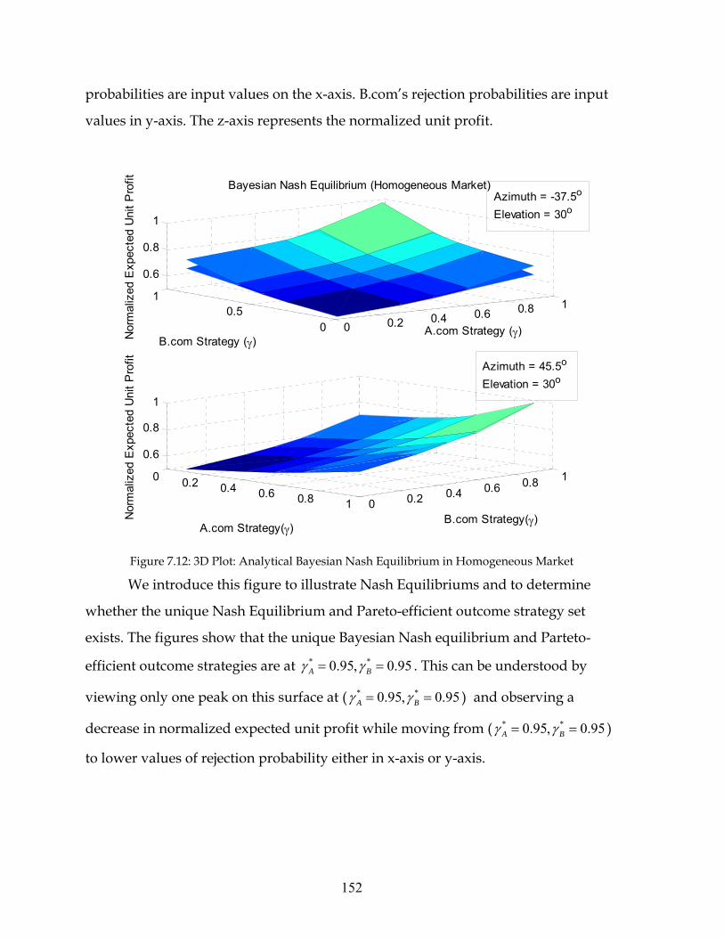
The dissertation concludes that our approach achieves a relative advantage in profit over the classical Bertrand model for both the homogeneous and heterogeneous service-based Internet markets. Our model yields positive profit for all providers and decreases the market price of services relative to customers’ budgets while guaranteeing their preferences. The novel model optimizes profit of providers in one or multiple Bayesian-Nash equilibriums and the Paretro-efficient outcomes subject to the network architecture, traffic pattern, service class mix, and strategies available. Providers achieve fair market shares with these equilibriums. In addition to the profit optimization, providers can implement our method to perform least price routing, traffic load balancing, capacity planning, and service provisioning.
1.2 BACKGROUND RESEARCH ON NETWORK PRICING ................................................... 21 1.2.1 Service per Customers’ Bids........................................................................... 21 1.2.2 Static Congestion Game.................................................................................. 21 1.2.3 Provider’s Monopolist Game.......................................................................... 22 1.2.4 Peer Providers in a Series .............................................................................. 23 1.2.5 Game of Incomplete Information in Sealed Bid Reverse Auction................... 23 1.2.6 Transaction-level Pricing Network Architecture............................................ 24
1.3 PROBLEM STATEMENT AND PROPOSED SOLUTION................................................... 25 1.3.1 The Proposed Price Transaction Architecture and Protocol ......................... 26 1.3.2 Proposed Providers’ Game of Oligopoly ....................................................... 28 1.3.3 Proposed method of Optimizing Providers’ Profit ......................................... 29 1.3.4 Proposed Algorithm........................................................................................ 31 1.3.5 Research Methods........................................................................................... 31
1.4 DISTINGUISHING CHARACTERISTIC OF OUR APPROACH............................................ 33 1.5 SUMMARY OF CONTRIBUTION.................................................................................. 36 1.6 STRUCTURE OF THE DISSERTATION.......................................................................... 37
2 NETWORK ARCHITECTURE AND PROTOCOL ................................................ 38
3 PROVIDERS’ GAME OF OLIGOPOLY .................................................................. 55
3.1 MODEL SELECTION .................................................................................................. 55 3.2 SERVICE CLASS AND ENTERPRISE PREFERENCE....................................................... 59 3.3 MODEL PARAMETERS .............................................................................................. 62
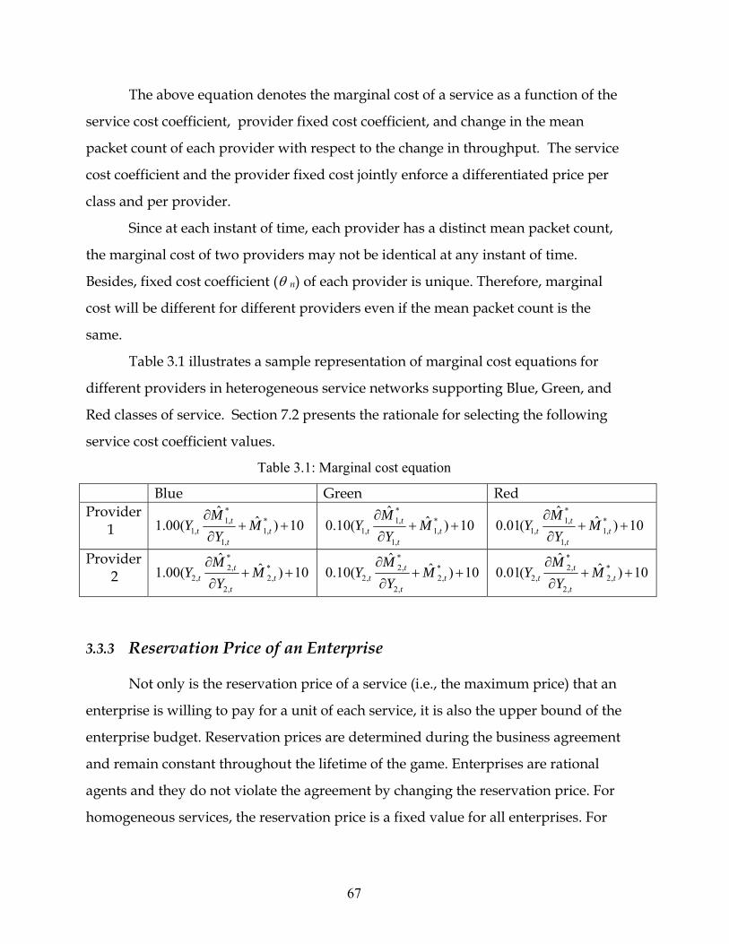
3.3.1 Market Capacity and Market Demand Functions .......................................... 62 3.3.2 Marginal Cost Function.................................................................................. 64 3.3.3 Reservation Price of an Enterprise................................................................. 67 3.3.4 Profit Function................................................................................................ 69
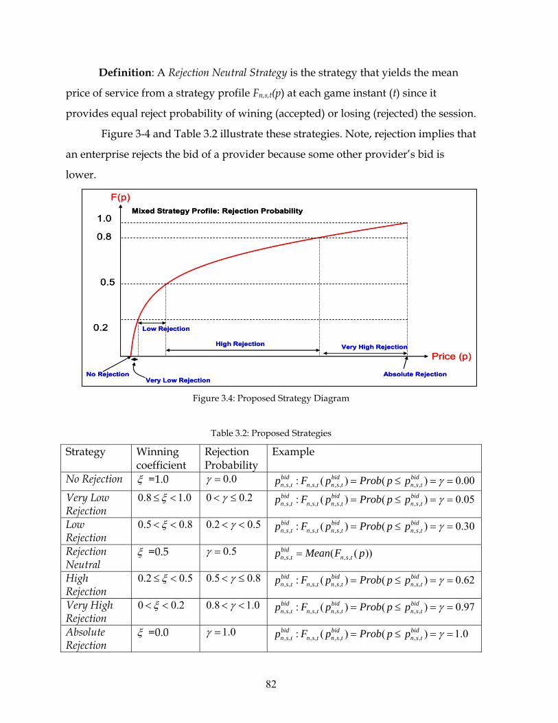
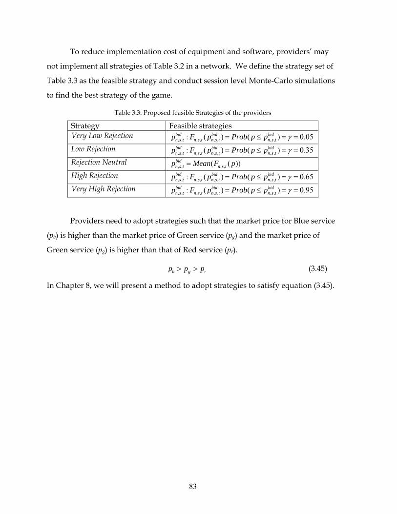
3.4 PROPOSED OLIGOPOLY MODEL................................................................................ 71 3.5 THE MOVEMENT OF THE BELIEF FUNCTION............................................................. 77 3.6 PROVIDERS’ STRATEGIES......................................................................................... 79 3.7 CHAPTER SUMMARY................................................................................................ 84
4 PROVIDERS’ PROFIT MAXIMIZATION BY OPTIMUM ROUTING.............. 85
4.1 NETWORK ARCHITECTURE CONSTRAINTS ............................................................... 88 4.2 TRAFFIC PATTERN AND QUEUE SYSTEM CONSTRAINTS........................................... 89 4.3 MEAN PACKET COUNT IN THE M/M/1 MODEL ......................................................... 91 4.4 SESSION ARRIVAL DISTRIBUTION ............................................................................ 92 4.5 THE DEVELOPMENT OF A NON-LINEAR OPTIMIZATION PROGRAM........................... 92 4.6 CHAPTER SUMMARY................................................................................................ 97
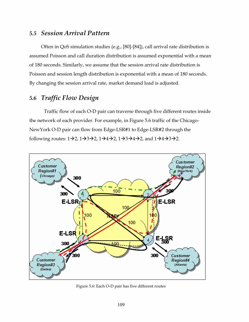
5 NETWORK AND TRAFFIC FLOW DESIGN.......................................................... 98
6 A SNAPSHOT OF THE ALGORITHM................................................................... 116
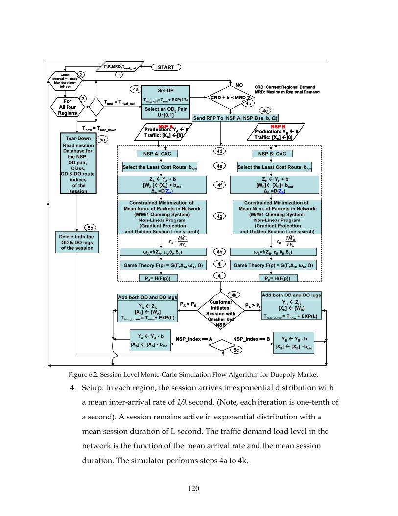
6.1 THE LAYERED VIEW OF THE ALGORITHM .............................................................. 116 6.2 PERFORMANCE MEASUREMENT METRICS.............................................................. 118 6.3 SESSION LEVEL MONTE-CARLO SIMULATION ALGORITHM ................................... 119
7 MATHEMATICAL ANALYSES AND VALIDATION .......................................... 123
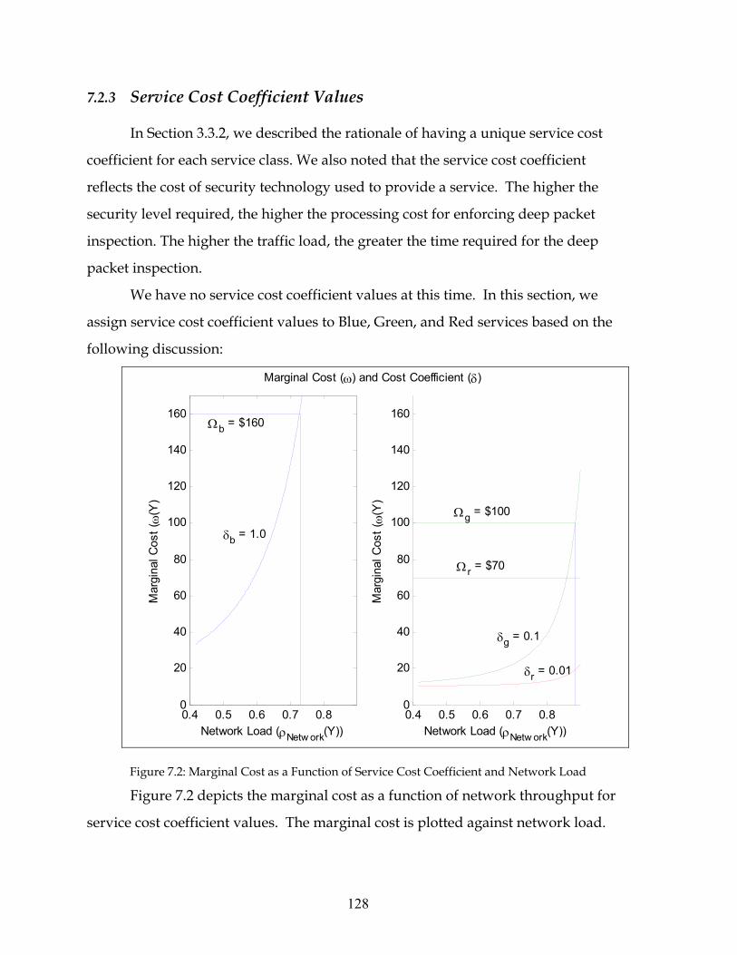
7.1 THE RESERVATION PRICE ...................................................................................... 124 7.2 SERVICE COST COEFFICIENT VALUES IN MARGINAL COST.................................... 124
7.2.1 Analytical Marginal Cost Function .............................................................. 125 7.2.2 Simulated Marginal Cost Function............................................................... 127 7.2.3 Service Cost Coefficient Values .................................................................... 128
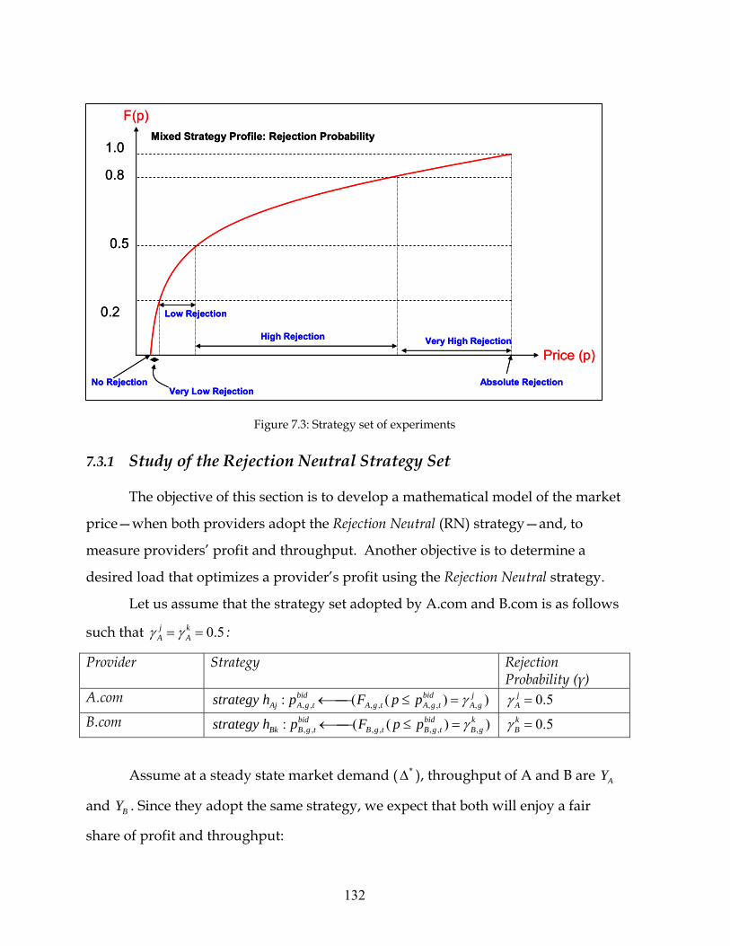
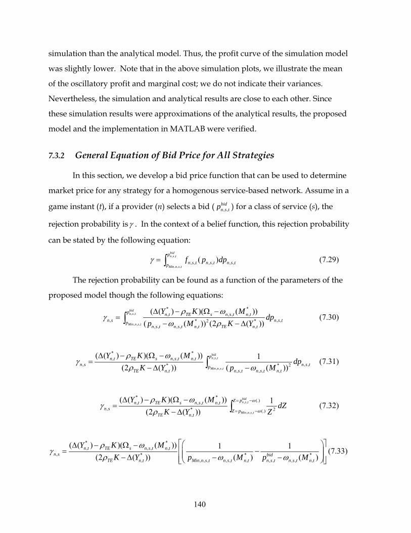
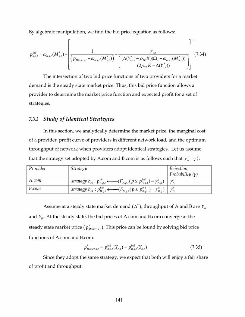
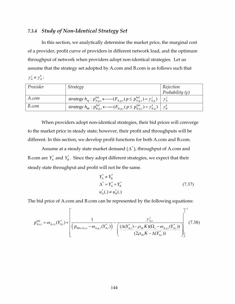
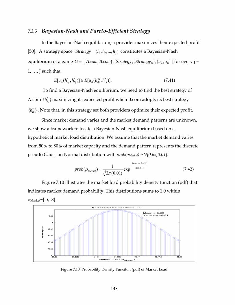
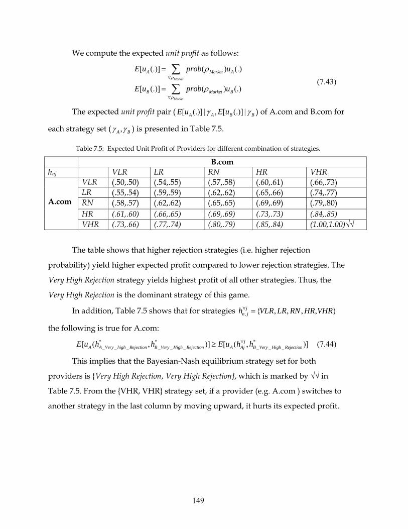
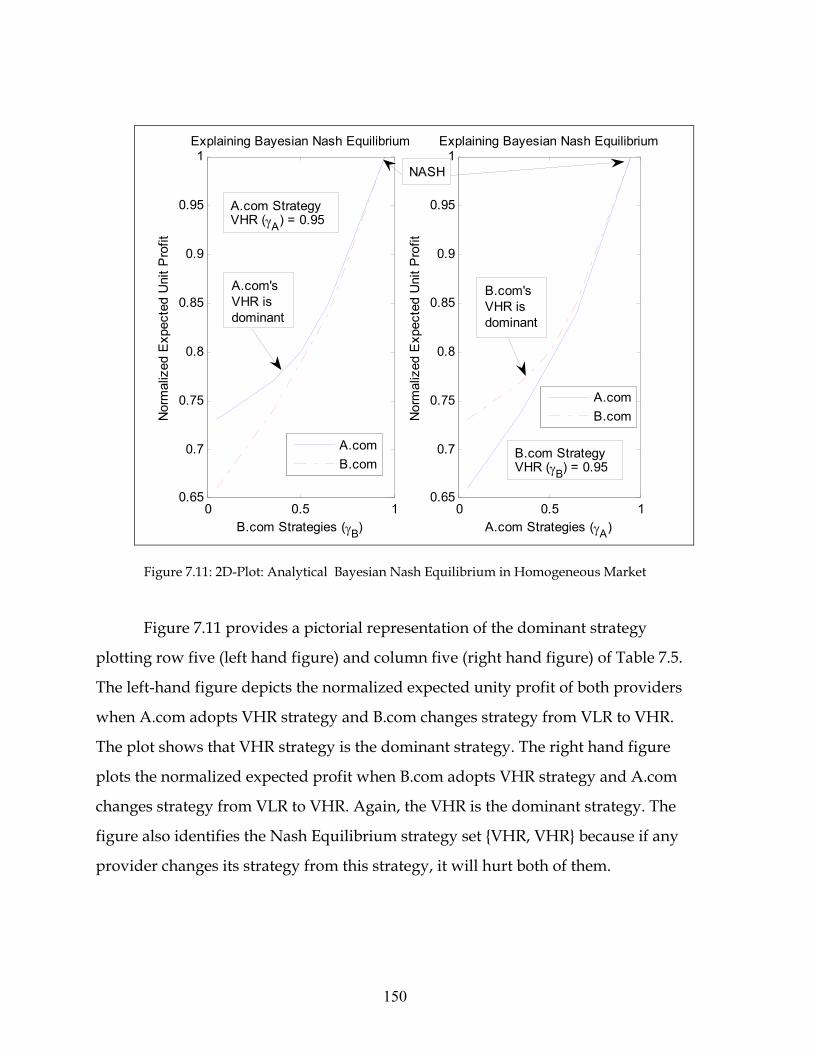
7.3.1 Study of the Rejection Neutral Strategy Set .................................................. 132 7.3.2 General Equation of Bid Price for All Strategies ......................................... 140 7.3.3 Study of Identical Strategies ......................................................................... 141 7.3.4 Study of Non-Identical Strategy Set .............................................................. 144 7.3.5 Bayesian-Nash and Pareto-Efficient Strategy .............................................. 148
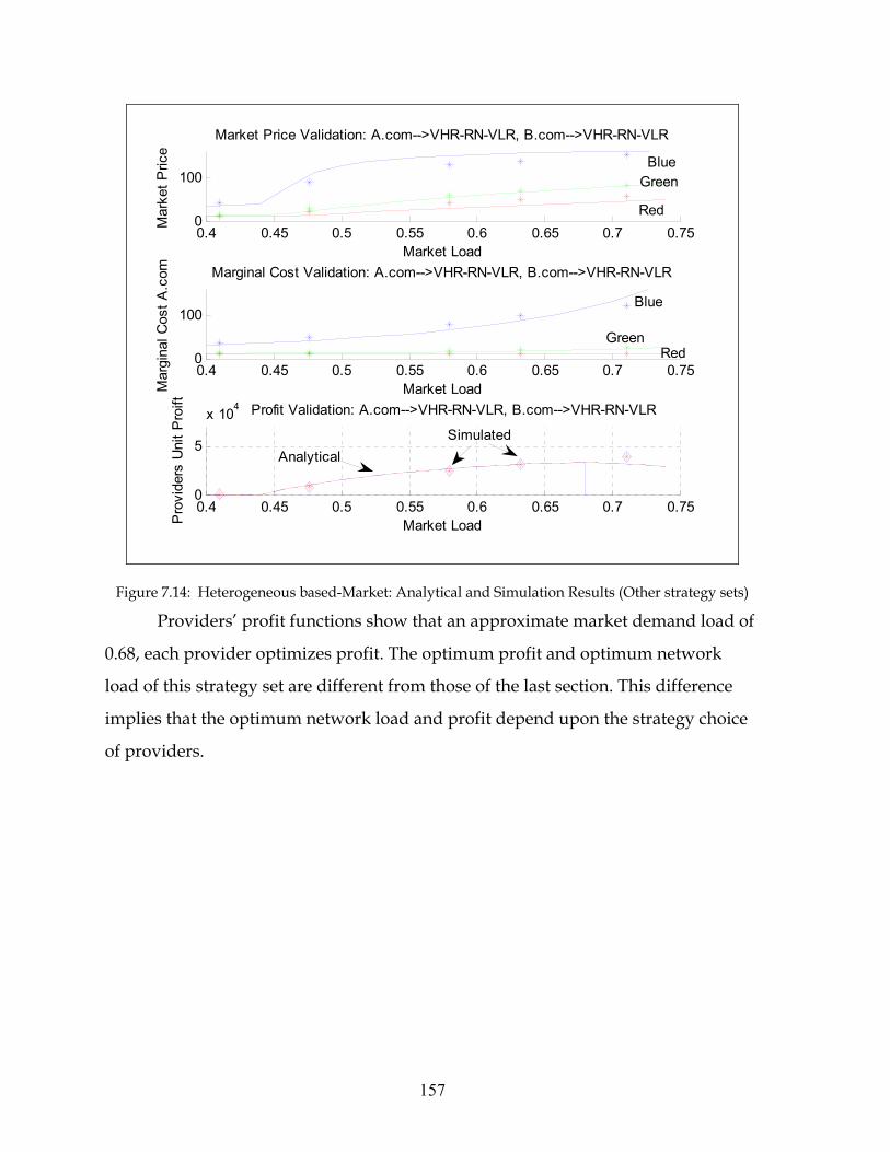
7.4 HETEROGENEOUS SERVICE-BASED MARKET.......................................................... 153 7.4.1 Study of Identical Strategy Set ...................................................................... 153
7.4.1.1 The Rejection Neutral Strategy Set........................................................... 154 7.4.1.2 Study of Other Strategy Sets..................................................................... 156
7.4.2 Non-Identical Strategy Set ............................................................................ 158 7.5 CHAPTER SUMMARY.............................................................................................. 159
8 SESSION LEVEL MONTE-CARLO SIMULATION, APPLICATIONS, AND
8.1.4.1 Finding a Safe Strategy............................................................................. 167 8.1.4.2 Finding Pareto-Efficient Outcome Strategy Set ....................................... 171 8.1.4.3 The Routing Scheme................................................................................. 177 8.1.4.4 Traffic Load Adjustment........................................................................... 179
8.1.5 Advantage of the Model ................................................................................ 182 8.2 HETEROGENEOUS SERVICE-BASED MARKET.......................................................... 184
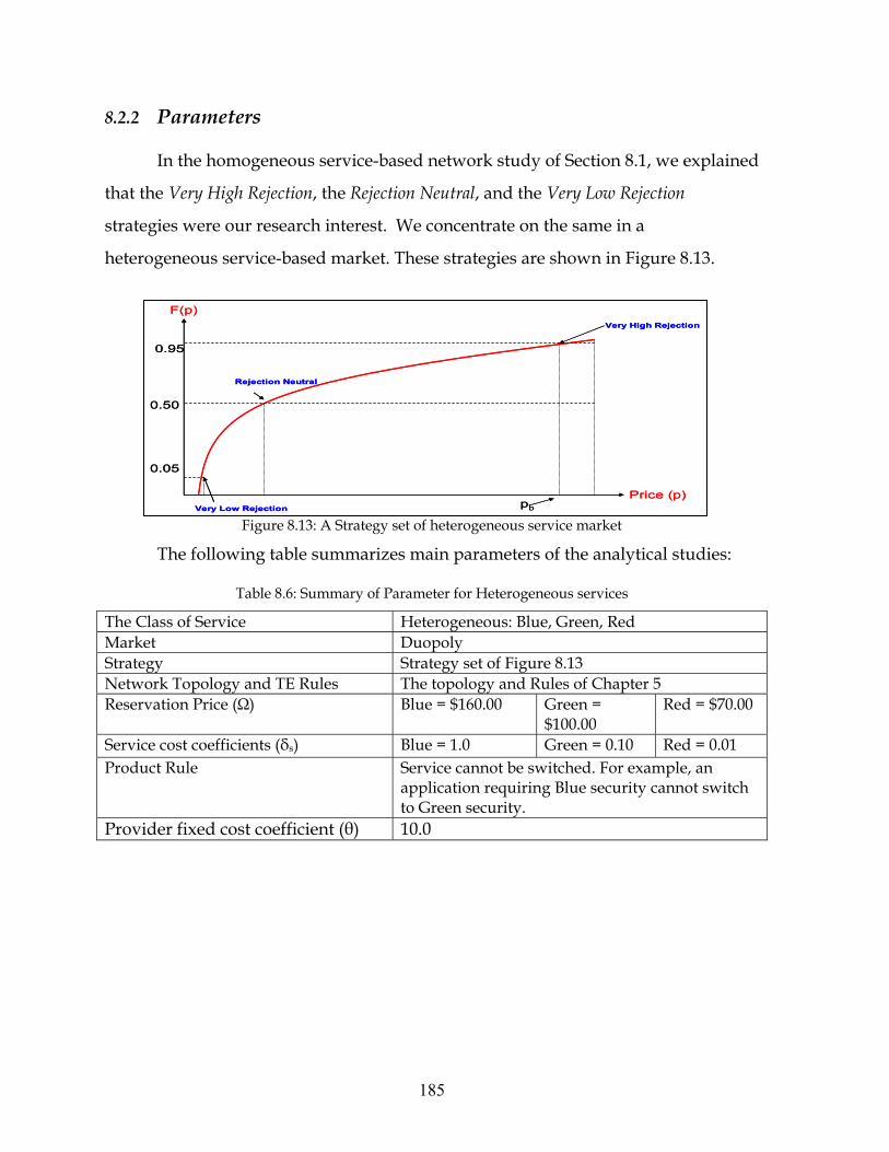
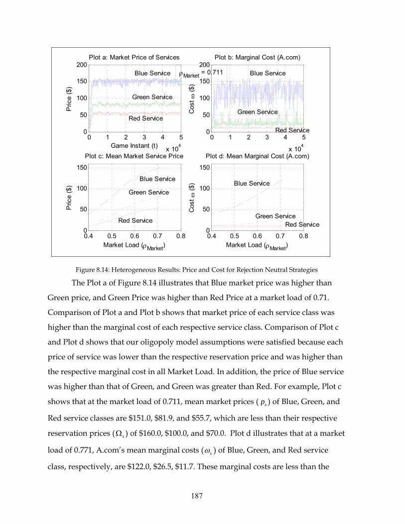
8.2.1 Experiment Objectives .................................................................................. 184 8.2.2 Parameters.................................................................................................... 185 8.2.3 Validation of the model................................................................................. 186
8.2.5 Advantage of the Model ................................................................................ 206 8.3 CHAPTER SUMMARY.............................................................................................. 207
9.1 SUMMARY OF CONTRIBUTIONS .............................................................................. 210 9.1.1 A Novel Automatic Price Transaction Architecture ..................................... 210 9.1.2 An Extension of the Current ATIS and 3GPP Architecture.......................... 210 9.1.3 Session Initiation Protocol based Price Transaction Protocol .................... 211 9.1.4 The Providers Optimized Game in Internet Traffic ...................................... 211 9.1.5 An Analytical Model, a Network Model, and a Session Level Monte-Carlo Simulator 212 9.1.6 A Framework to Determine the Best Preferred Strategy.............................. 213
9.2 LIMITATIONS.......................................................................................................... 214 9.2.1 Traffic Distribution Pattern .......................................................................... 214 9.2.2 The Cost Function......................................................................................... 214 9.2.3 Network Queue Model .................................................................................. 215
9.3 ADVANTAGE .......................................................................................................... 215 9.3.1 Improvement on Classical Models................................................................ 215 9.3.2 Automation of Pricing and Billing................................................................ 216 9.3.3 Synthesis of Game Theory and Traffic Engineering Techniques.................. 216 9.3.4 Implementation of Strategies ........................................................................ 217
THE NECESSARY AND SUFFICIENT CONDITIONS................................................................ 233 THE GRADIENT PROJECTION ALGORITHM.......................................................................... 234 THE GOLDEN SECTION LINE SEARCH................................................................................. 235
APPENDIX B:LIST OF ACRONYMS............................................................................. 237
10
Figures
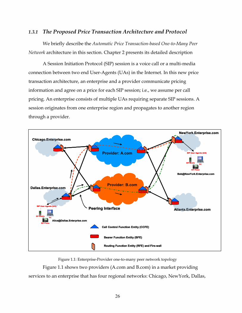
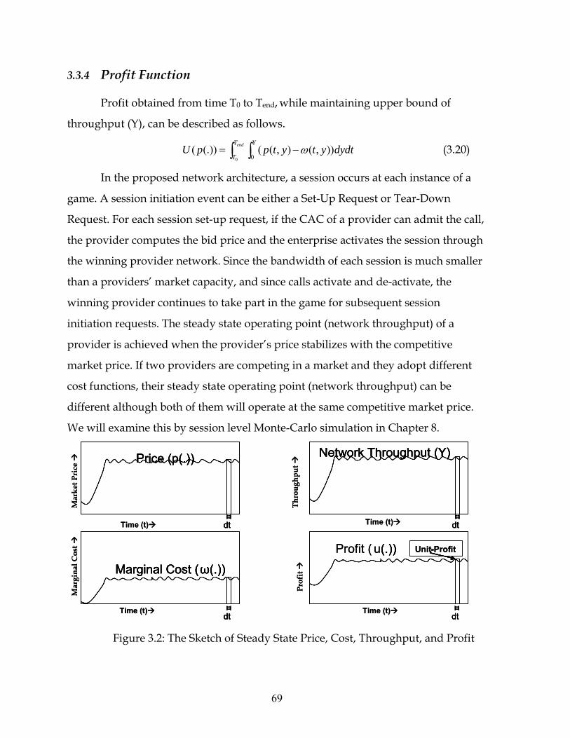
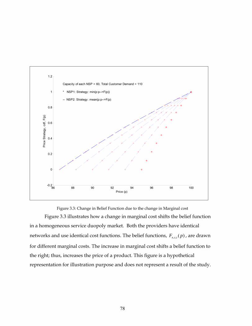
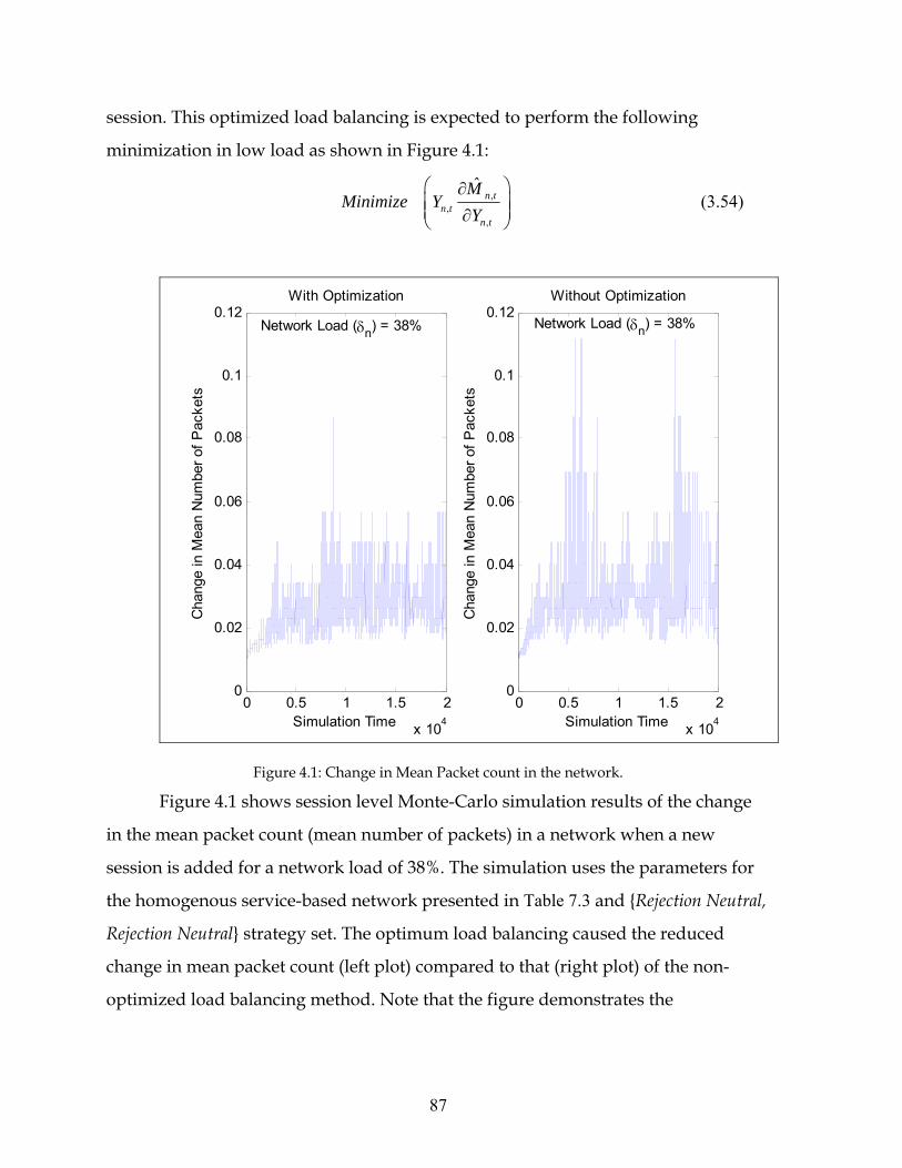
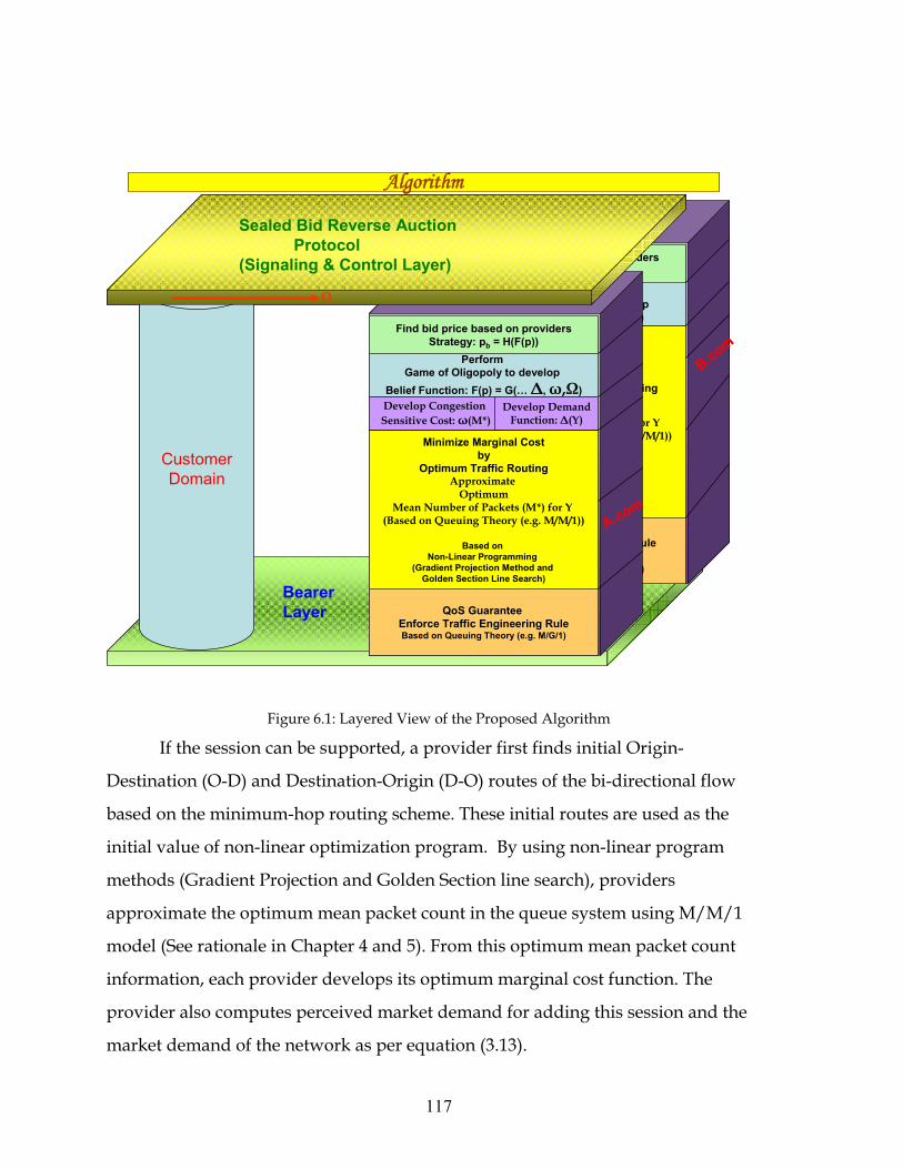
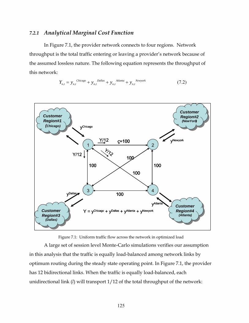
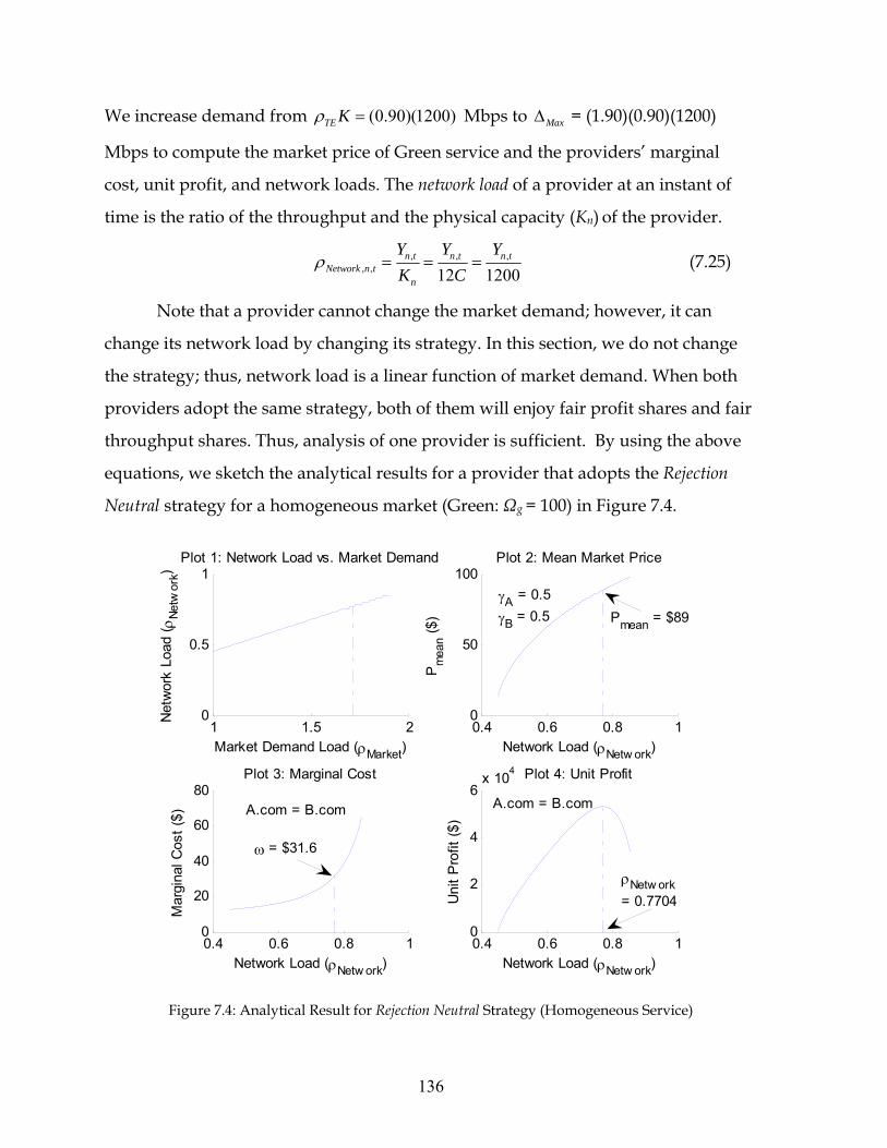
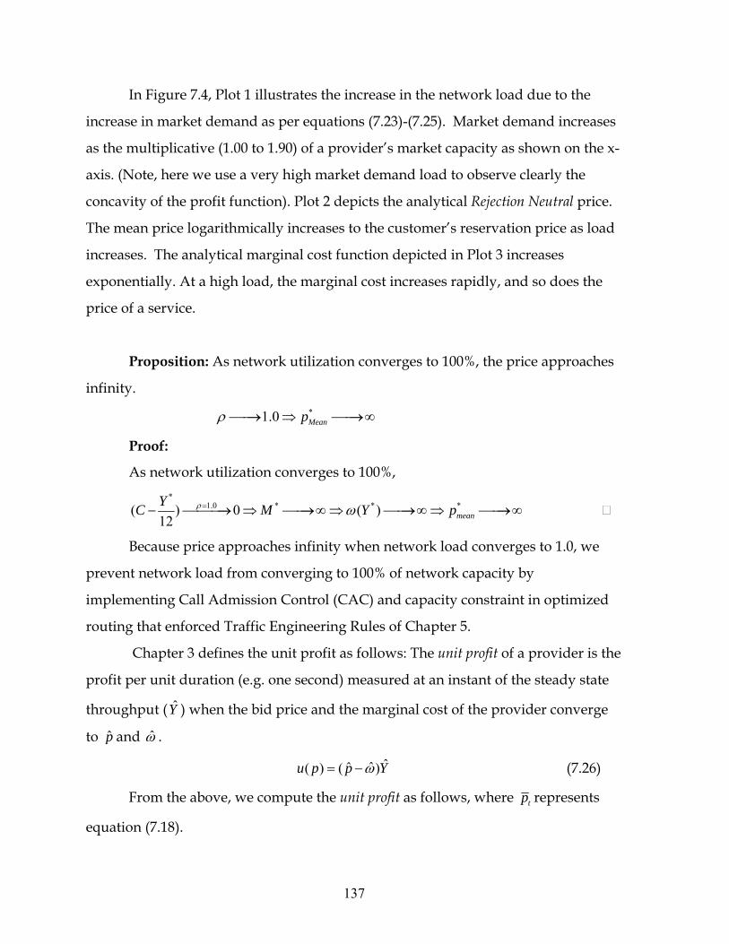
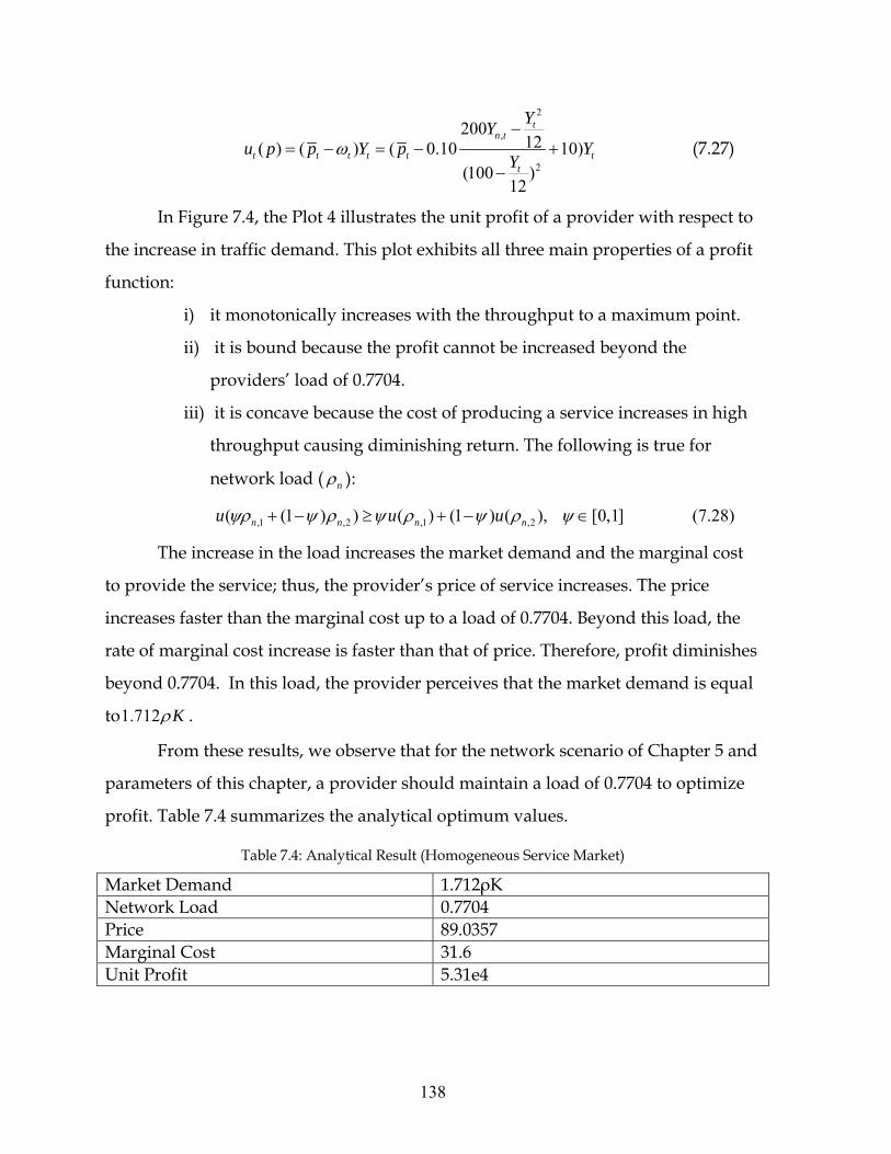
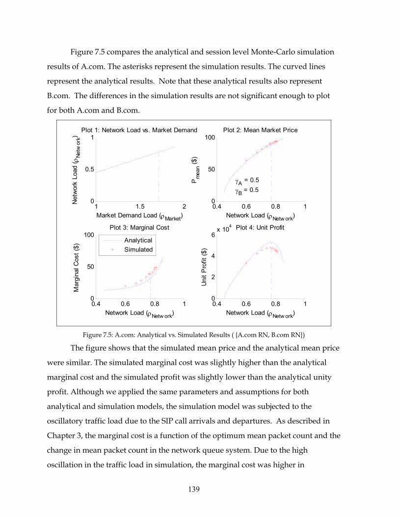
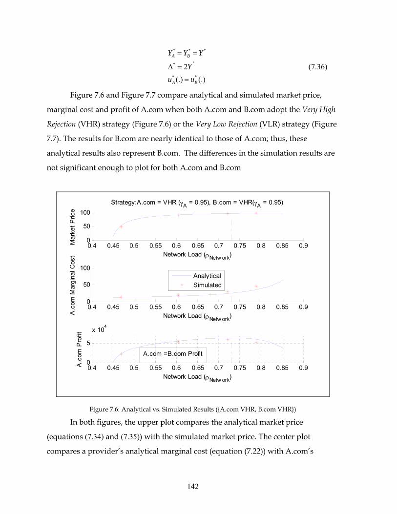
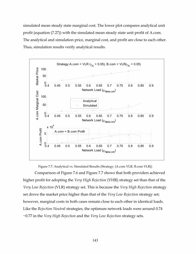
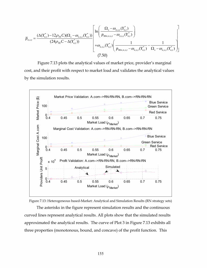
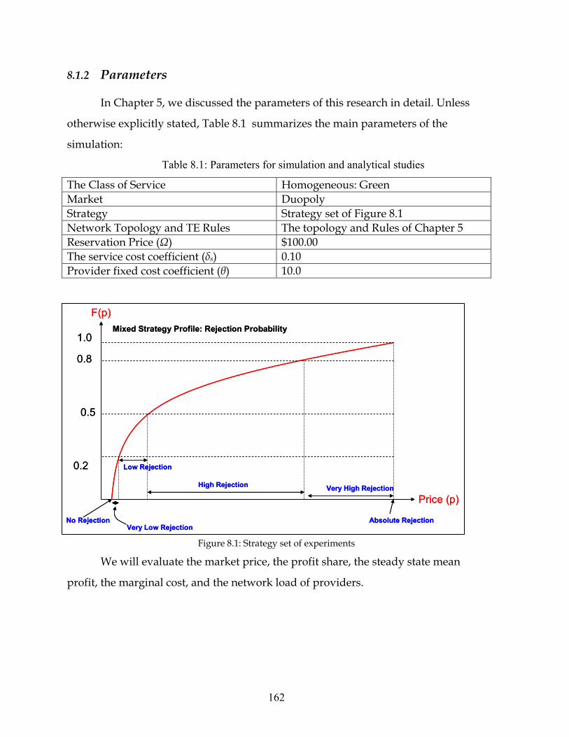
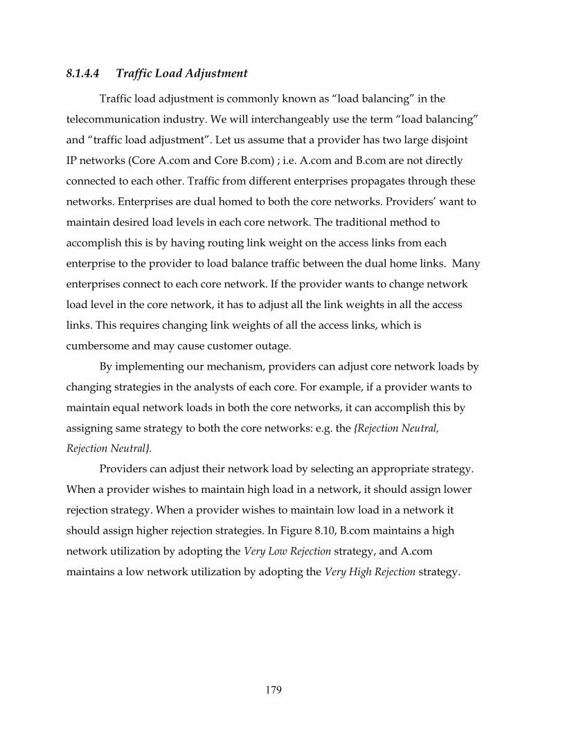
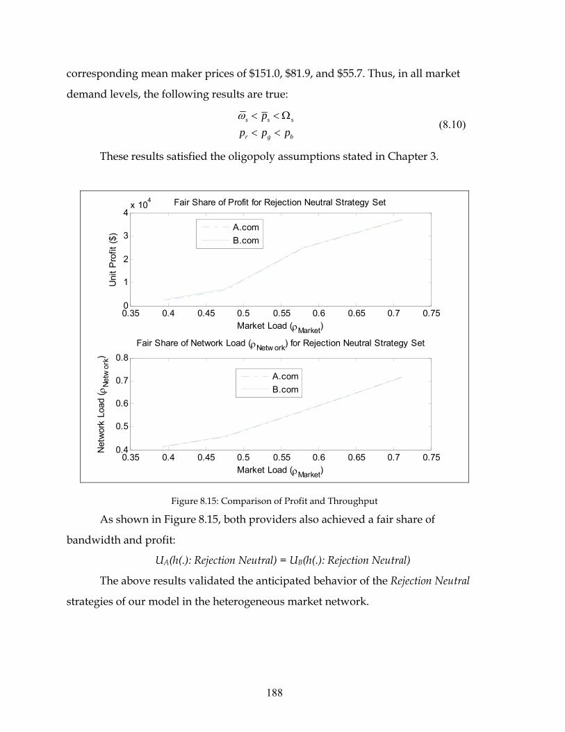
1.1: Enterprise-Provider one-to-many peer network topology ..................................................................26 2.1: Session Initiation Protocol Entities.....................................................................................................40 2.2: ATIS/PTSC IP Peering Reference Diagram.......................................................................................42 2.3: Network Architecture of Duopoly Market ..................................................................................44 2.4: 3GPP IMS Architecture ......................................................................................................................46 2.5: The current 3GPP IMS Online Charging Architecture.......................................................................46 2.6: 3GPP Online Charging System...........................................................................................................47 2.7: Extended 3GPP Charging Architecture in Duopoly Market ..............................................................48 2.8: Price Transaction Protocol..................................................................................................................51 2.9: Session Initiation Protocol (SIP) Control Flow ..................................................................................53 3.1: Demand Function................................................................................................................................64 3.2: The Sketch of Steady State Price, Cost, Throughput, and Profit...............................................69 3.3: Change in Belief Function due to the change in Marginal cost..........................................................78 3.4: Proposed Strategy Diagram ................................................................................................................82 4.1: Change in Mean Packet count in the network. ...................................................................................87 5.1: Simulation topology ........................................................................................................................99 5.2: VoIP Packet Length ..........................................................................................................................100 5.3: Single Integrated FIFO Queue system..............................................................................................103 5.4: M/G/1 System Delay for Heterogeneous services............................................................................105 5.5: Internal Network Topology of Two providers..................................................................................107 5.6: Each O-D pair has five different routes ............................................................................................109 6.1: Layered View of the Proposed Algorithm........................................................................................117 6.2: Session Level Monte-Carlo Simulation Flow Algorithm for Duopoly Market................................120 7.1: Uniform traffic flow across the network in optimized load.............................................................125 7.2: Marginal Cost as a Function of Service Cost Coefficient and Network Load .................................128 7.3: Strategy set of experiments...............................................................................................................132 7.4: Analytical Result for Rejection Neutral Strategy (Homogeneous Service) .....................................136 7.5: A.com: Analytical vs. Simulated Results ( A.com RN, B.com RN) ......................................139 7.6: Analytical vs. Simulated Results (A.com VHR, B.com VHR) ....................................................142 7.7: Analytical vs. Simulated Results (Strategy: A.com VLR, B.com VLR) ......................................143 7.8: Solving Non-Identical Strategies Bid Price Equations by Numerical Analysis ...............................146 7.9: Comparison of Dissimilar strategies.................................................................................................147 7.10: Probability Density Funciton (pdf) of Market Load.......................................................................148 7.11: 2D Plot—Analytical Bayesian Nash Equilibrium in Homogeneous Market .................................150 7.12: 3D Plot—Analytical Bayesian Nash Equilibrium in Homogeneous Market .................................152 7.13: Heterogeneous based-Market: Analytical and Simulation Results (RN strategy sets)...................155 7.14: Heterogeneous based-Market: Analytical and Simulation Results (Other strategy sets) ..............157 8.1: Strategy set of experiments...............................................................................................................162 8.2: Simulation Result: Comparison of Random Rejection and Rejection Neutral Strategies. .......165 8.3: Comparison of all strategies with the Rejection Neutral strategy ............................................168 8.4: Very High and Neutral strategy providers’ load and marginal cost .................................................169
11
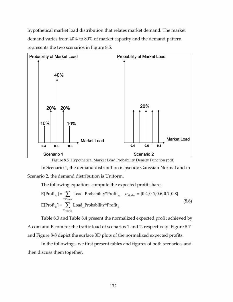
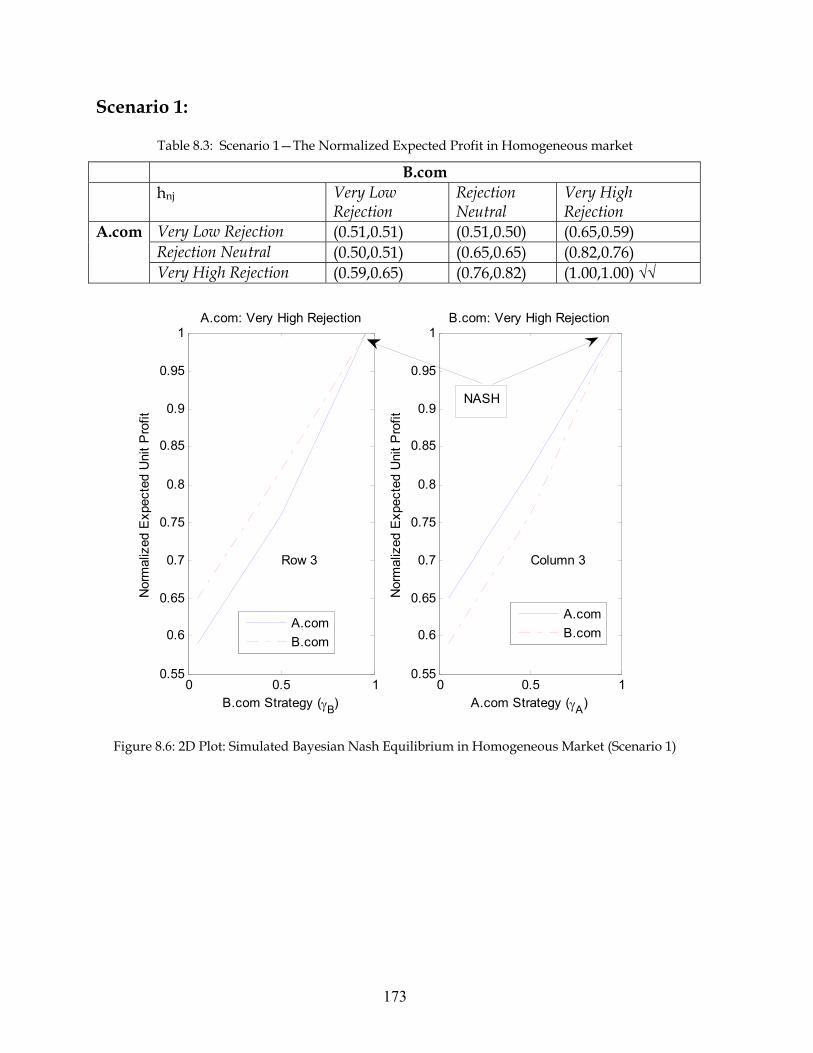
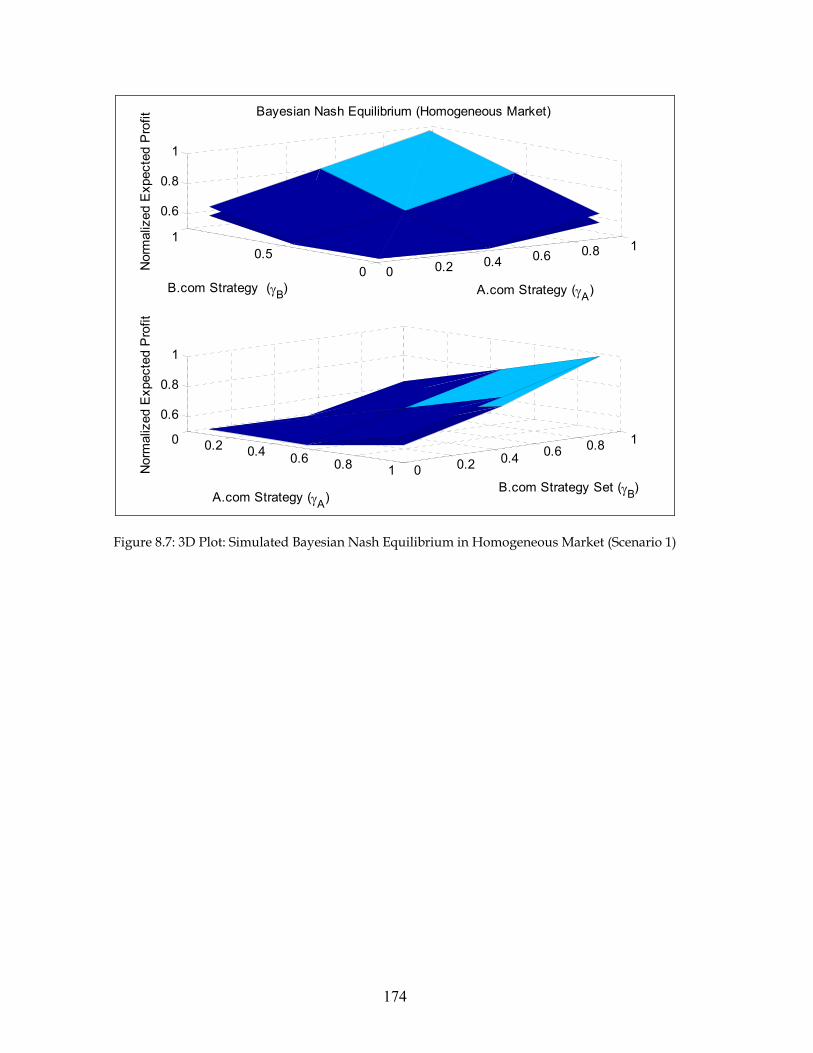
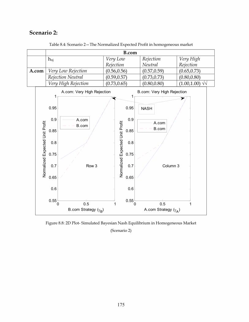
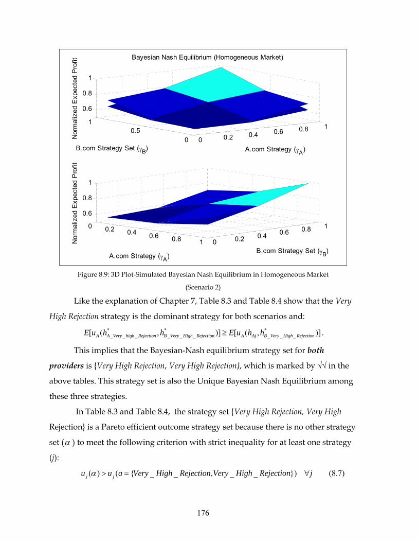
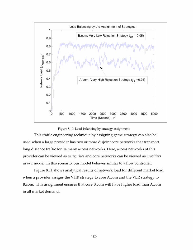
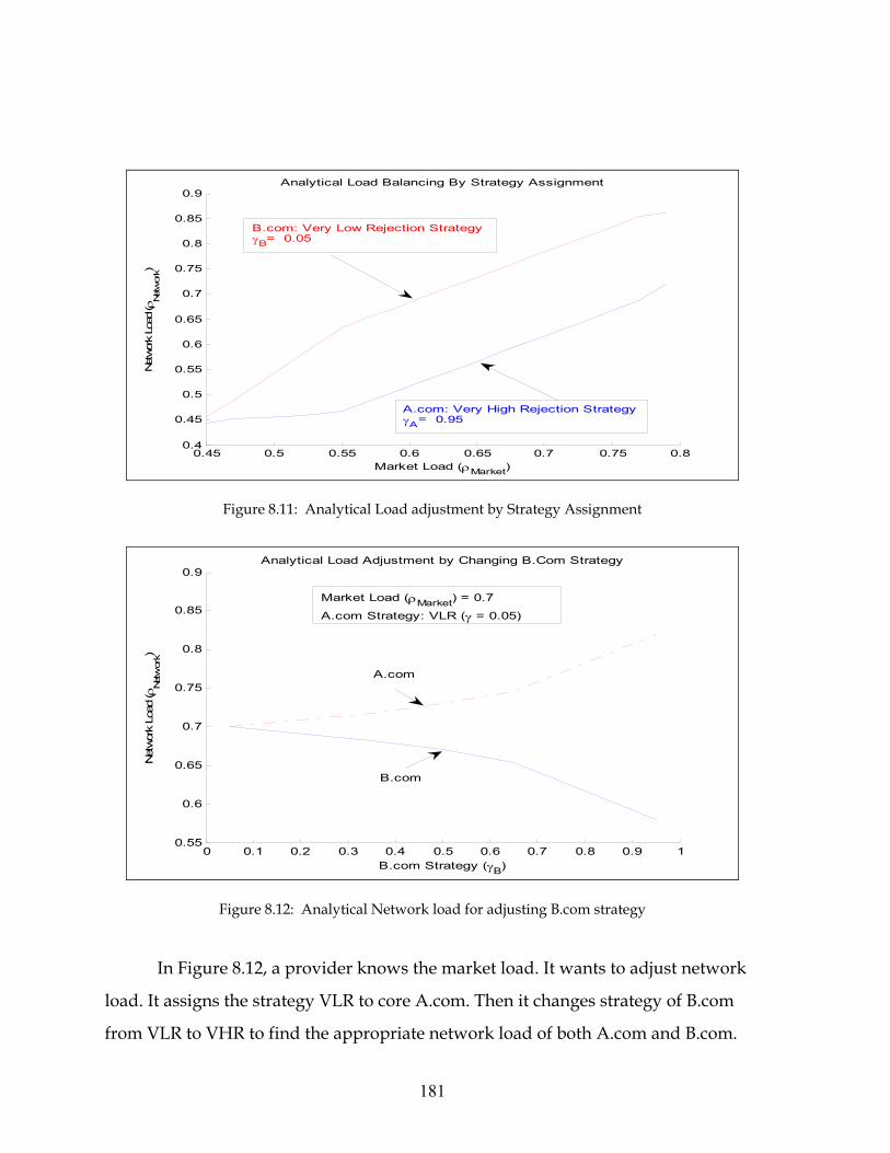
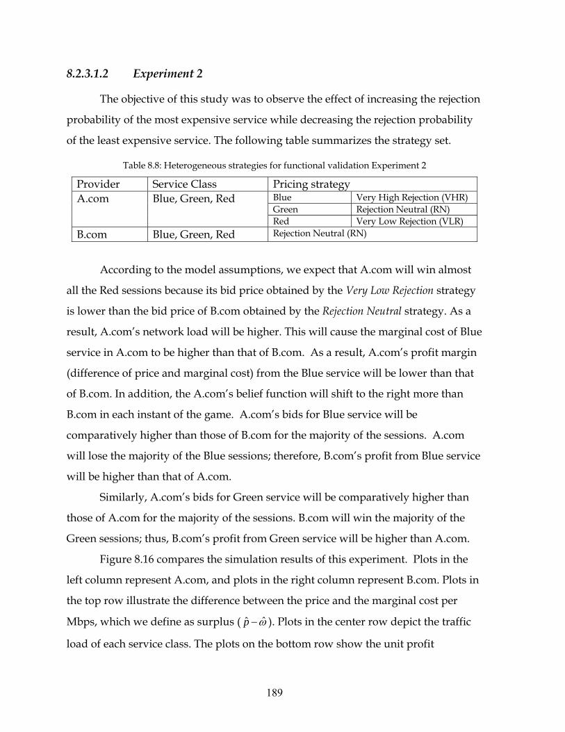
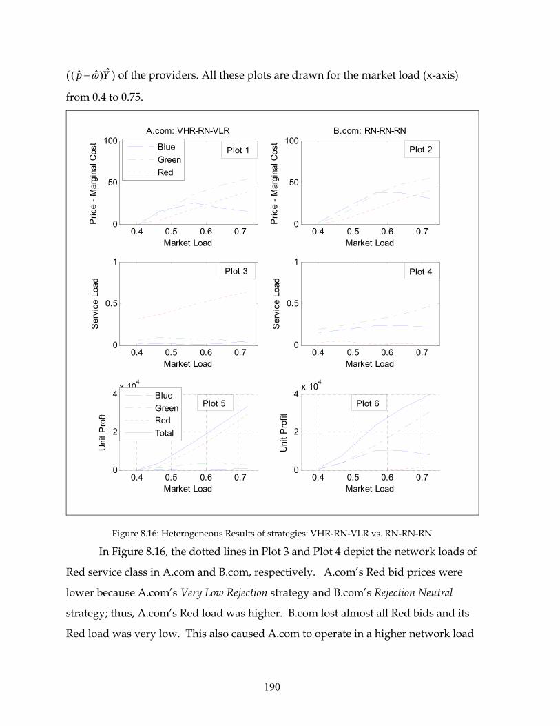
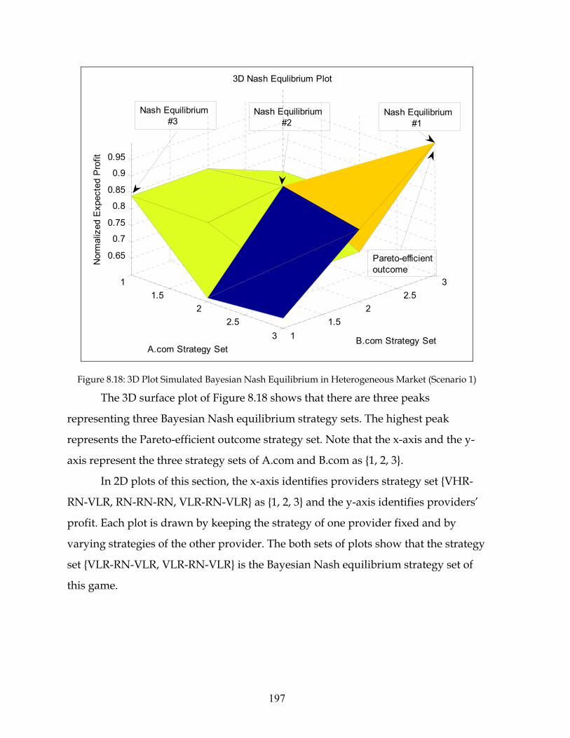
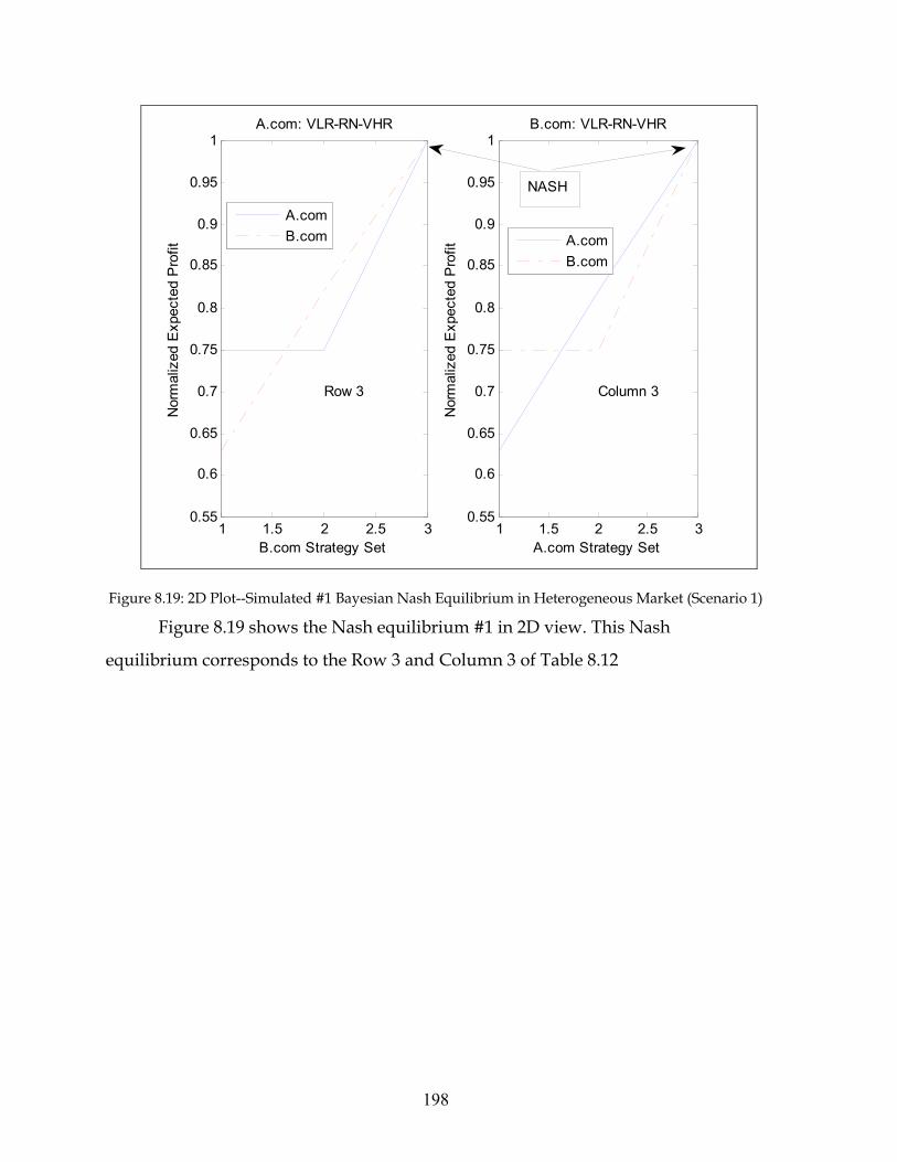
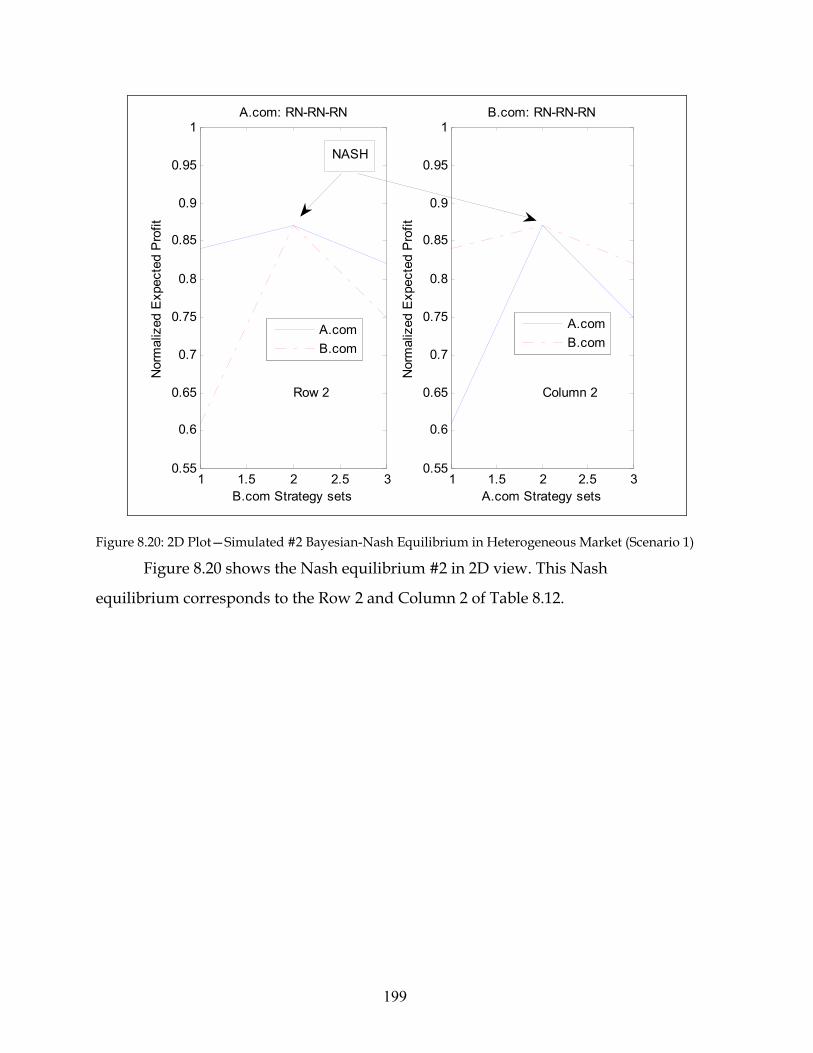
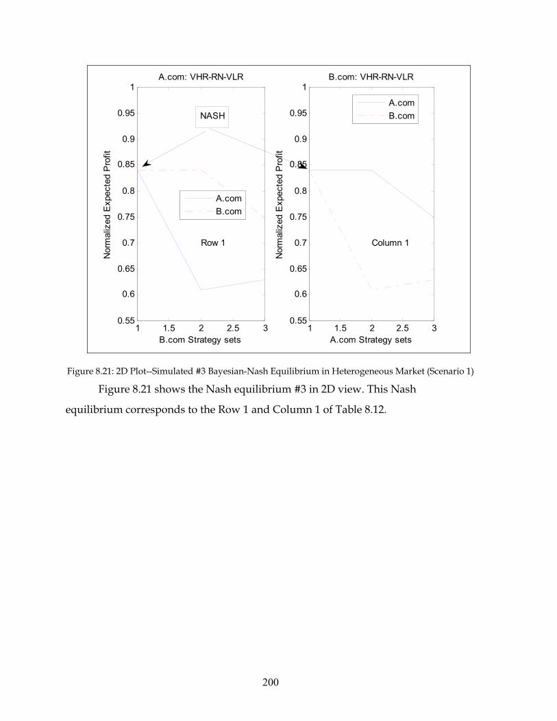
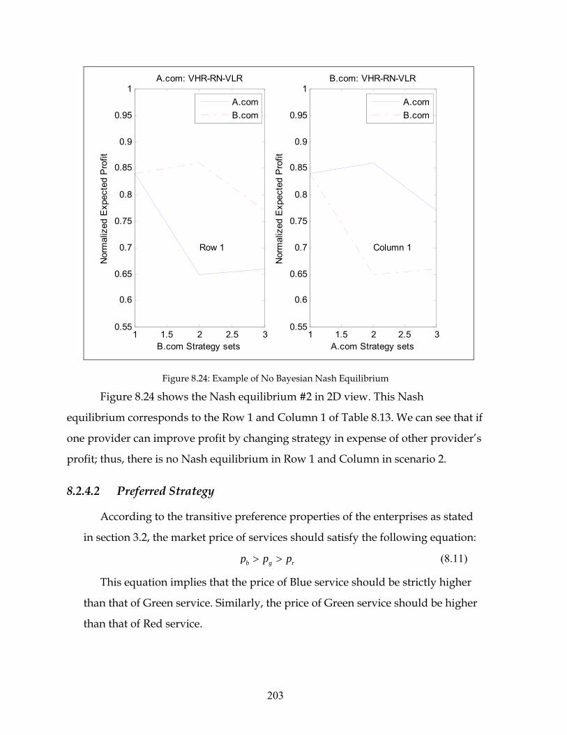
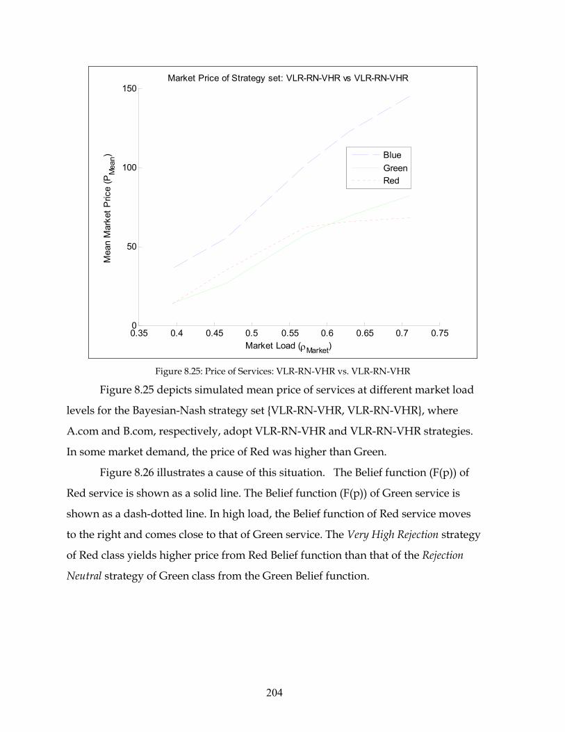
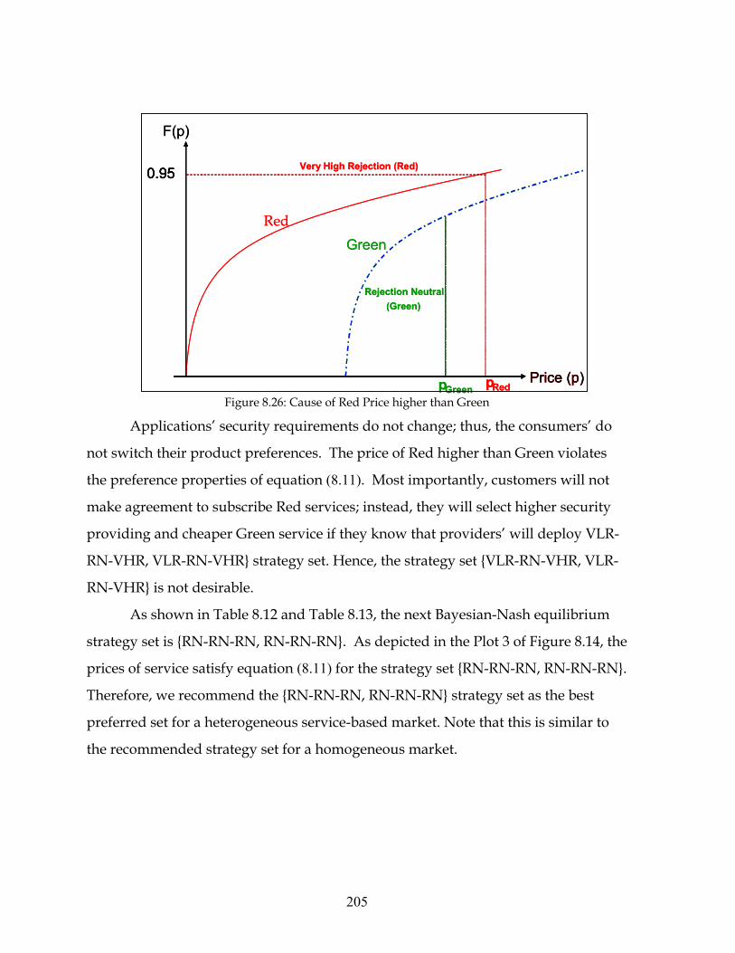
8.5: Hypothetical Market Load Probability Density Function (pdf)........................................................172 8.6: 2D Plot: Simulated Bayesian Nash Equilibrium in Homogeneous Market (Scenario 1) .................173 8.7: 3D Plot: Simulated Bayesian Nash Equilibrium in Homogeneous Market (Scenario 1) .................174 8.8: 2D Plot- Simulated Bayesian Nash Equilibrium in Homogeneous Market......................................175 8.9: 3D Plot-Simulated Bayesian Nash Equilibrium in Homogeneous Market ...........................176 8.10: Load balancing by strategy assignment ..........................................................................................180 8.11: Analytical Load adjustment by Strategy Assignment....................................................................181 8.12: Analytical Network load for adjusting B.com strategy .................................................................181 8.13: A Strategy set of heterogeneous service market.............................................................................185 8.14: Heterogeneous Results: Price and Cost for Rejection Neutral Strategies ......................................187 8.15: Comparison of Profit and Throughput............................................................................................188 8.16: Heterogeneous Results of strategies: VHR-RN-VLR vs. RN-RN-RN...........................................190 8.17: Heterogeneous Results of strategies: VLR-RN-VHR vs. RN-RN-RN...........................................193 8.18: 3D Plot—Simulated Bayesian Nash Equilibrium in Heterogeneous Market (Scenario 1) ............197 8.19: 2D Plot—Simulated #1 Bayesian Nash Equilibrium in Heterogeneous Market (Scenario 1) .......198 8.20: 2D Plot—Simulated #2 Bayesian-Nash Equilibrium in Heterogeneous Market (Scenario 1) .......199 8.21: 2D Plot—Simulated #3 Bayesian-Nash Equilibrium in Heterogeneous Market (Scenario 1) .......200 8.22: 2D Plot—Simulated #1 Bayesian-Nash Equilibrium in Heterogeneous Market (Scenario 2) .......201 8.23: 2D Plot—Simulated #2 Bayesian Nash Equilibrium in Heterogeneous Market (Scenario 2) .......202 8.24: Example of No Bayesian Nash Equilibrium...................................................................................203 8.25: Price of Services: VLR-RN-VHR vs. VLR-RN-VHR................................................................204 8.26: Cause of Red Price higher than Green............................................................................................205
12
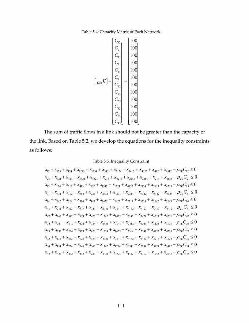
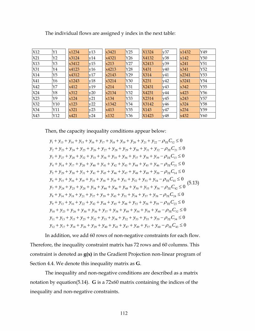
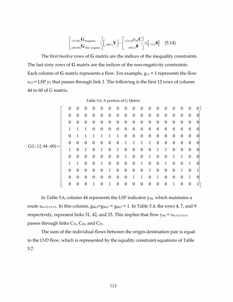
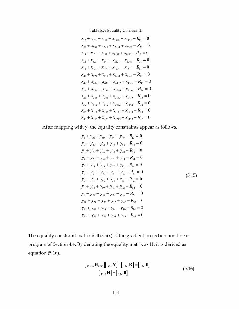
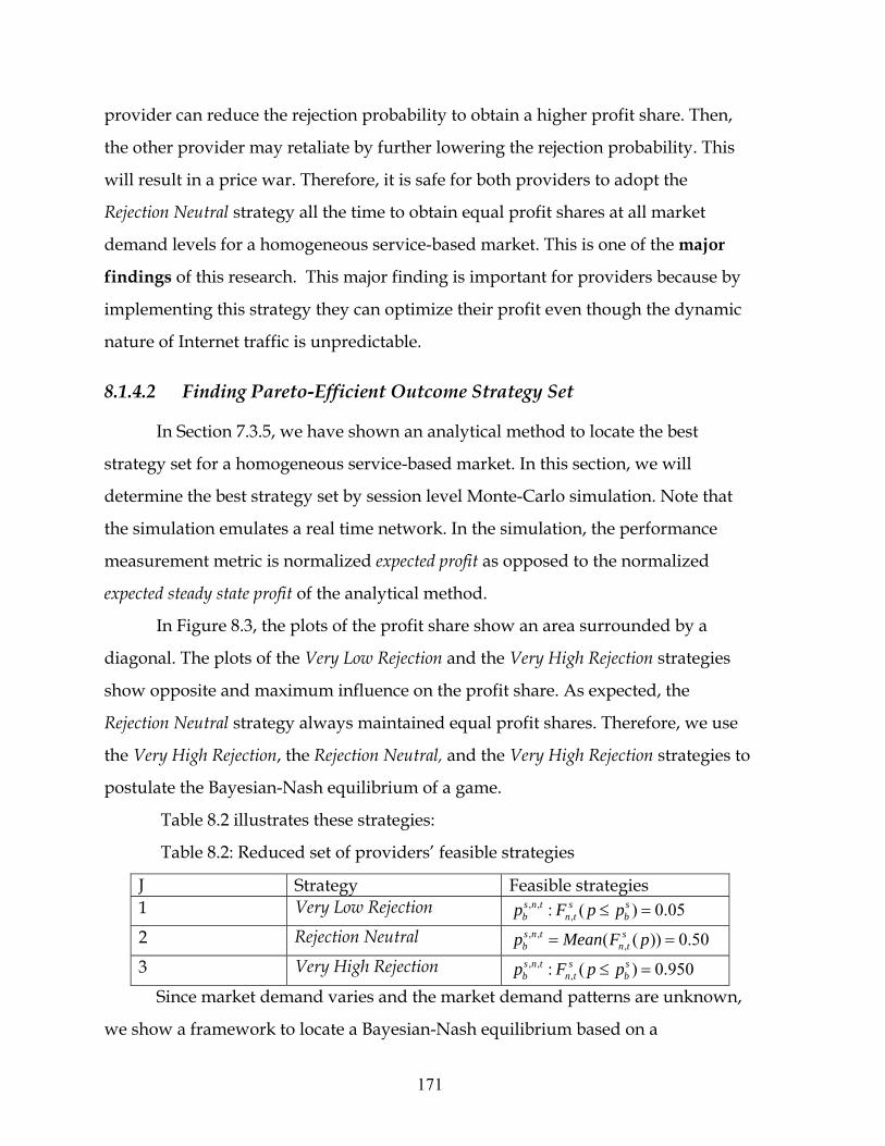
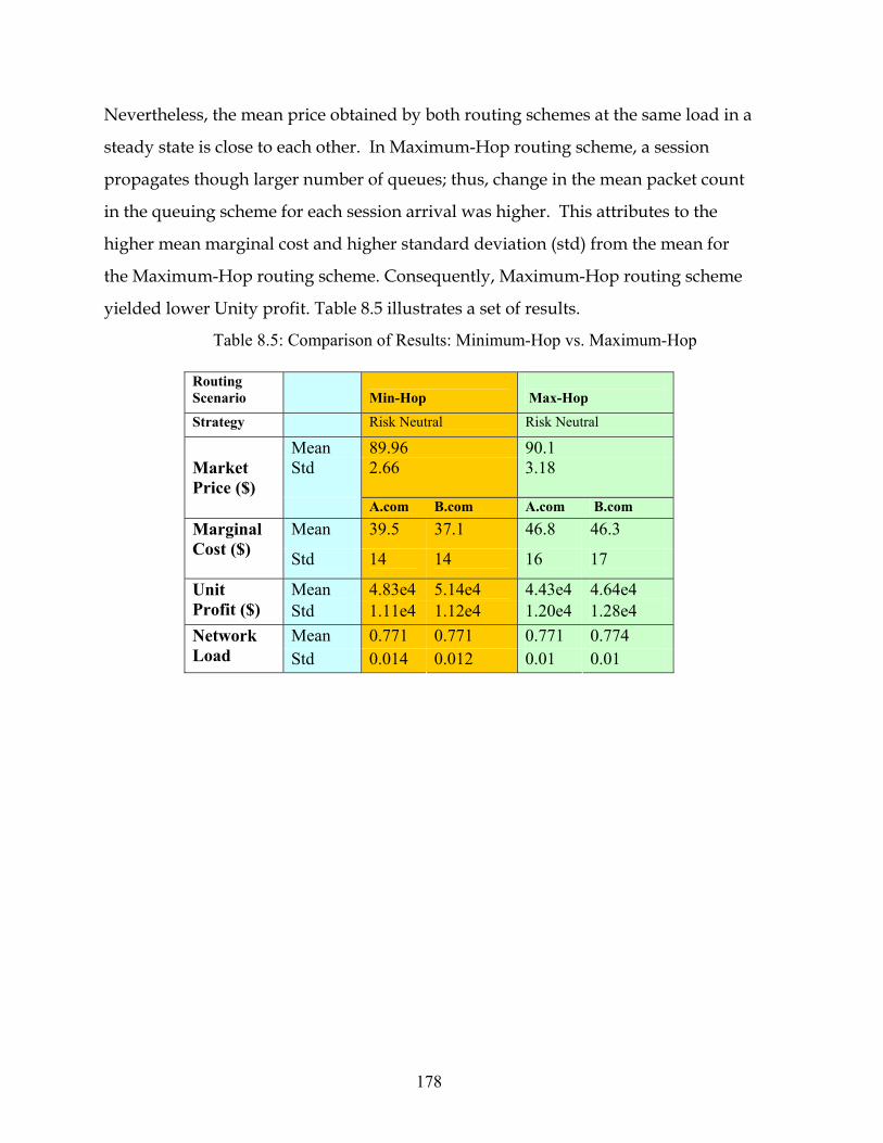
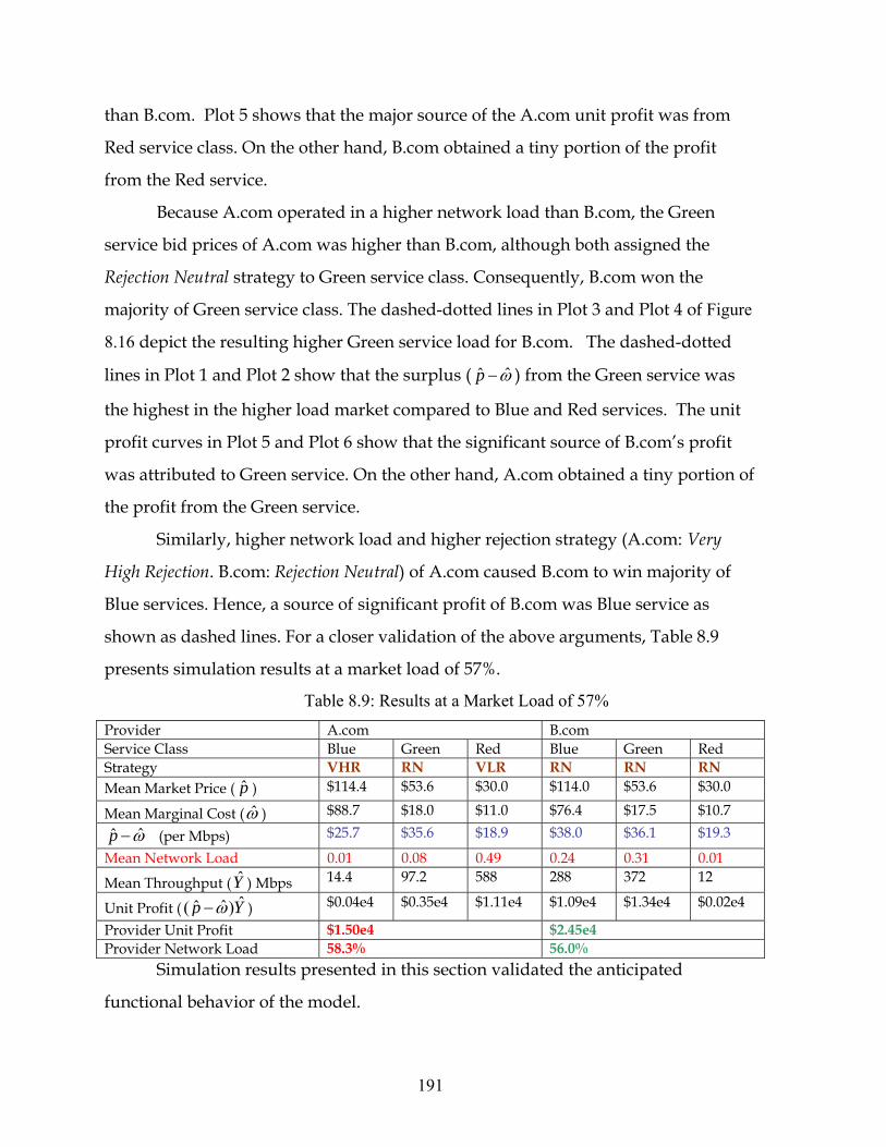
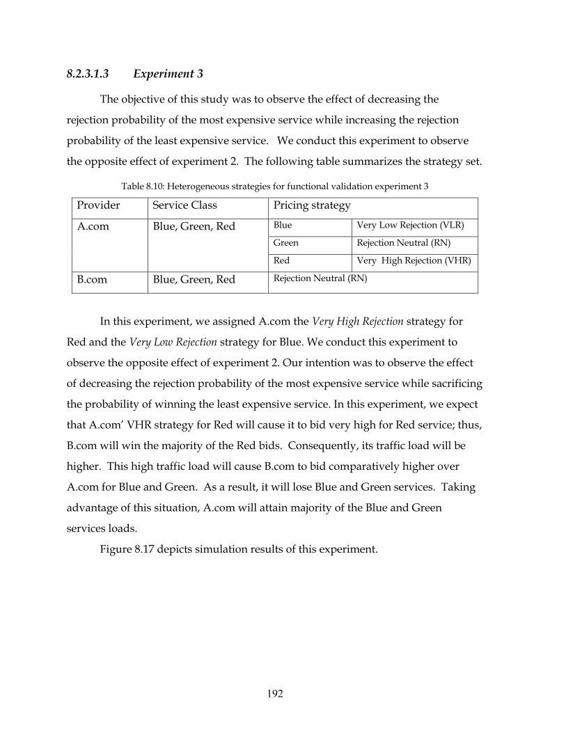
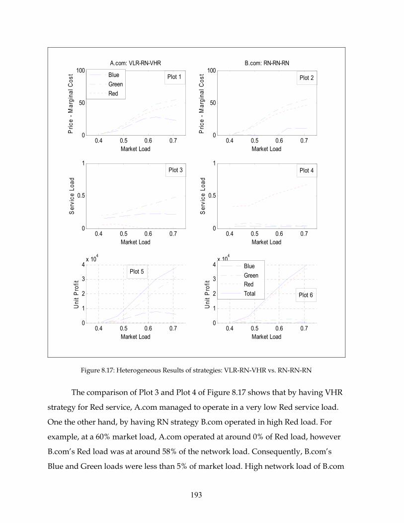
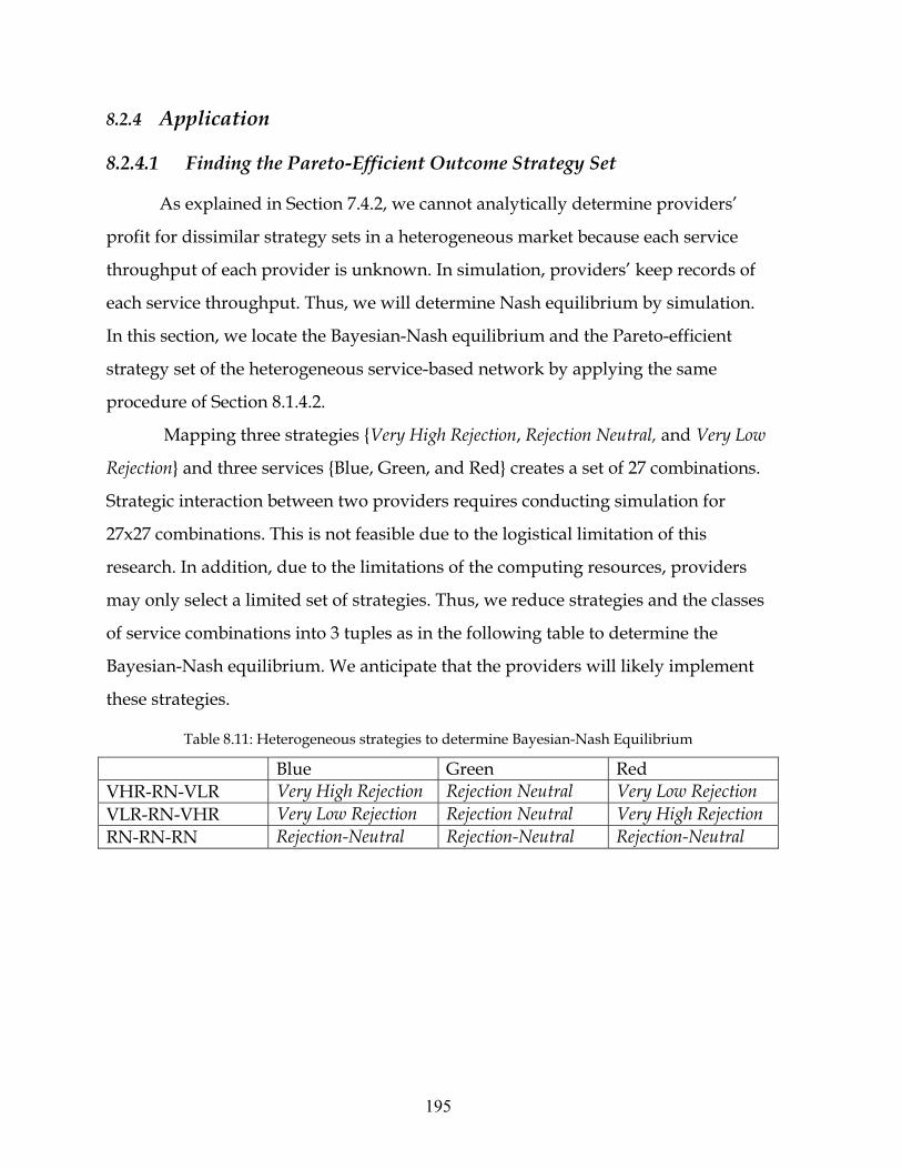
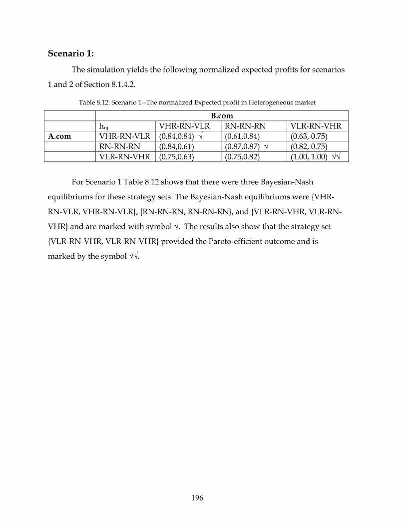
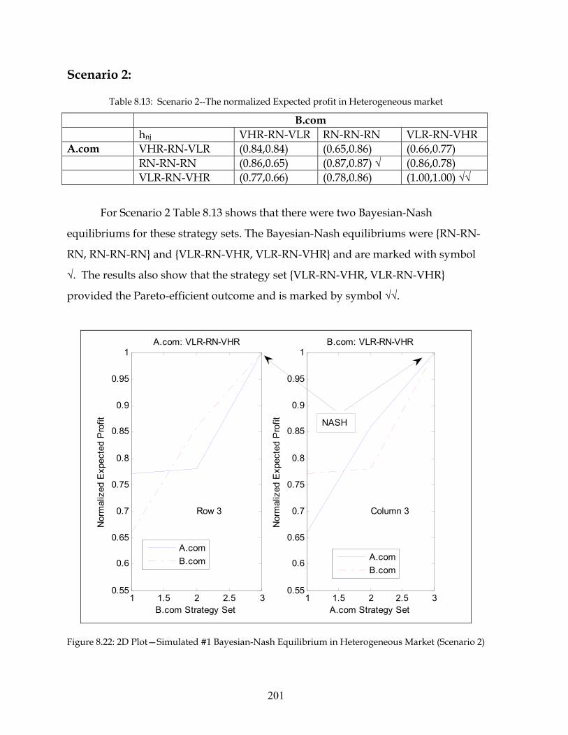
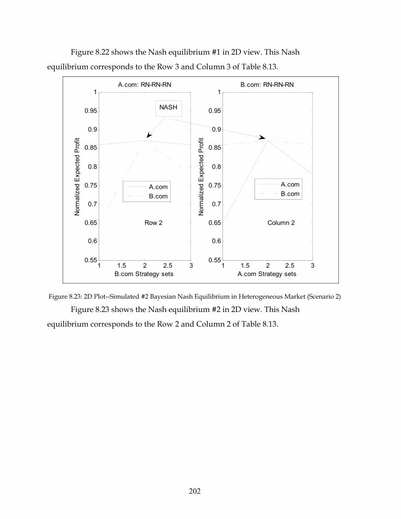
Tables 1.1: Classes of Games ............................................................................................................. 17 2.1: 3GPP IMS Functional Components................................................................................. 45 2.2: Components of different types of networks..................................................................... 50 3.1: Marginal cost equation..................................................................................................... 67 3.2: Proposed Strategies.......................................................................................................... 82 3.3: Proposed feasible Strategies of the providers .................................................................. 83 5.1: Capacity Assignment ..................................................................................................... 108 5.2: O-D pairs and paths ....................................................................................................... 110 5.3: O-D Traffic Matrix ........................................................................................................ 110 5.4: Capacity Matrix of Each Network ................................................................................. 111 5.5: Inequality Constraint...................................................................................................... 111 5.6: A portion of G Matrix.................................................................................................... 113 5.7: Equality Constraints....................................................................................................... 114 7.1: The Reservation price of different types of services ..................................................... 124 7.2: The Service Cost Coefficient values.............................................................................. 130 7.3: Parameters for homogeneous service-based network.................................................... 131 7.4: Analytical Result (Homogeneous Service Market) ....................................................... 138 7.5: Expected Unit Profit of Providers for different combination of strategies................... 149 7.6: Summary of Parameter for Heterogeneous services...................................................... 153 8.1: Parameters for simulation and analytical studies........................................................... 162 8.2: Reduced set of providers’ feasible strategies................................................................. 171 8.3: Scenario 1—The Normalized Expected Profit in Homogeneous market ..................... 173 8.4: Scenario 2—The Normalized Expected Profit in homogeneous market ....................... 175 8.5: Comparison of Results: Minimum-Hop vs. Maximum-Hop......................................... 178 8.6: Summary of Parameter for Heterogeneous services...................................................... 185 8.7: Heterogeneous strategies for functional validation experiment 1 ................................. 186 8.8: Heterogeneous strategies for functional validation Experiment 2................................. 189 8.9: Results at a Market Load of 57%................................................................................... 191 8.10: Heterogeneous strategies for functional validation experiment 3 ............................... 192 8.11: Heterogeneous strategies to determine Bayesian-Nash Equilibrium........................... 195 8.12: Scenario 1--The normalized Expected profit in Heterogeneous market...................... 196 8.13: Scenario 2--The normalized Expected profit in Heterogeneous market..................... 201
13
1 Introduction
Session Initiation Protocol (SIP) supported peer networks have recently
ascended to prominence among Internet service providers according to Yankee
Group reports [77]-[79]. Automating the price transaction for services and
optimizing profit of providers in such peer networks are recent challenges for
engineers. There is neither a well-established method, nor an automatic mechanism
for computing the service price in peer networks today.
Small providers are wholesale customers of large providers. These customers
want options for subscribing to services from large providers in one-to-many peer
networks with an automatic price transaction mechanism. They also desire to select
a provider instantaneously that offers the lowest price. Today, one-to-many peer
customers transport IP traffic through large providers based on the network load.
However, in our knowledge, no mechanism exists today for such transport based on
the service price.
Analogous to the desire of small providers, individual wireless customers
want to peer with multiple wireless providers and automatically subscribe to
services from the provider of their choice based on the service price.
We propose the new Automatic Price Transaction based One-to-Many Peer
Network architecture to meet customers’ desire for automatic price negotiations that
are concurrent with multiple providers. This architecture for one-to-many peer
networks supports a price transaction protocol, SIP entities and a SIP call flow. The
architecture allows customers to broadcast their budget and instantaneously
subscribe to the provider of their choice based on the competitive service price
analogous to the Sealed-Bid-Reverse auction [43][44]. Our model extends the one-to-
one IP peering architecture (IP Network-Network-Interface) of the Alliance for
Telecommunications and Industry Solutions (ATIS). Our model also extends the
14
one-to-one Online Charging architecture of the Third Generation Partnership Project
(3GPP).
Customers’ options of subscribing to any provider create strategic interaction
of price among the providers. This strategic interaction of the limited number of
providers and their attempt to optimize profit are the microeconomic concepts of
game theory in an oligopoly market [1][2]. Thus, we employ provider’s price
computation method using a game of oligopoly. Our game theory model is a
function of the peer traffic capacity and demand, the service cost, and a customer’s
budget.
Although the traffic capacity and a customer budget remain constant for a
relatively short duration of time, the traffic demand and the service cost vary due to
the dynamic nature of Internet traffic and the network congestion.
Large providers want to optimize their profit by automatic price computation
methods synchronized with the dynamic nature of Internet traffic demand in the
competitive market. The existing price computation mechanisms of providers are
not dynamic; i.e., the price is often asynchronous with the Internet traffic demand.
Providers’ marketing departments manually compute prices based on the historical
network load, market capacities, and traffic demand levels. By the time a marketing
department computes and advertises a new price, the network traffic pattern and
market demand may have already changed. Most importantly, the Internet traffic
demand is still unpredictable. This causes long reactive delays of price computation
that create an obstacle to selling services synchronized with the varying market
demand in the competitive market. Thus, there is a need for mechanisms that
automatically compute price synchronized with the Internet traffic demand and
sensitive to the network congestion.
We propose the new Providers Optimized Game in Internet Traffic model that
synthesizes a game theory, a traffic-engineering technique, and a non-linear
optimization method. The model allows providers to determine competitive price
synchronized with the dynamic Internet traffic demand and sensitive to the network
15
congestion. In this model, providers optimize profit by selecting strategically
sensitive price and by minimizing congestion sensitive network cost. A
mathematical non-linear program associated traffic engineering technique
minimizes the congestion sensitive network costs.
This dissertation presents the architecture and the model, validates them by
analyses and simulations, evaluates their advantages, determines providers best
game strategies that optimize their profit, and introduces traffic-engineering
applications.
The dissertation concludes that our approach—the implementation of the
architecture and the game model—achieves a relative advantage in profit over the
classical Bertrand model for both the homogeneous and heterogeneous service-
based Internet markets. Our approach yields positive profit for all providers and
decreases the market price of services relative to customers’ budget while
guaranteeing their preferences. The novel approach optimizes profit of providers in
one or multiple Bayesian-Nash equilibriums and the Paretro-efficient outcomes
subject to the network architecture, traffic pattern, service class mix, and strategies
available. Providers achieve fair market shares through these equilibriums. In
addition to the profit optimization, providers can implement our approach to
perform least price routing, traffic load distribution, capacity planning, and service
provisioning.
In the rest of this document, an enterprise is a small regional Internet Service
Provider (ISP) that has distributed networks across a continent, but does not have
national or international backbone networks. A provider is a large ISP that has
national and international backbone networks. An enterprise supports access
networks, sells services directly to consumers, and peers with providers to transport
its long distance and international traffic. A customer is either an enterprise or a
wireless customer. The price transaction protocol is for the customer-provider peer
interface to negotiate price.
16
We organize the rest of this chapter as follows. Section 1.1 briefly presents
microeconomic concepts such as optimizing providers’ profit and developing game
theory models. We study the outline of the related research in Section 1.2 to
comprehend the background of the problem. Section 1.3 presents the problem
statement, proposed solutions, and research methods. Section 1.4 discusses the
distinguishing characteristics of our approach. Section 1.5 provides a summary of
our contributions; and Section 1.6 outlines the document format.
1.1 Background Microeconomic Concepts
1.1.1 Profit
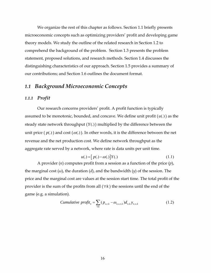
Our research concerns providers’ profit. A profit function is typically
assumed to be monotonic, bounded, and concave. We define unit profit ( (.)u ) as the
steady state network throughput ( (.)Y ) multiplied by the difference between the
unit price ( (.)p ) and cost ( (.)ω ). In other words, it is the difference between the net
revenue and the net production cost. We define network throughput as the
aggregate rate served by a network, where rate is data units per unit time.
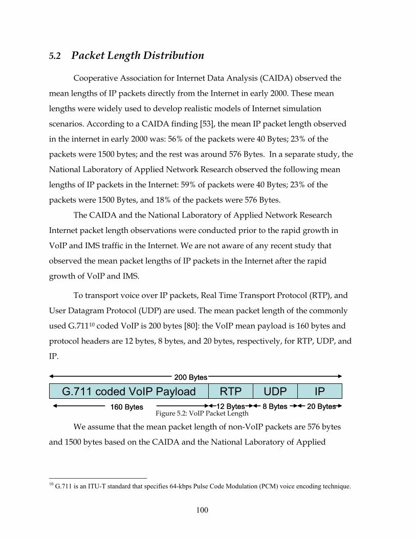
[ ](.) (.) (.) (.)u p Yω= − (1.1) A provider (n) computes profit from a session as a function of the price (p),
the marginal cost (ω), the duration (d), and the bandwidth (y) of the session. The
price and the marginal cost are values at the session start time. The total profit of the
provider is the sum of the profits from all ( k∀ ) the sessions until the end of the
game (e.g. a simulation).
, , , , , , , ,( )n s t k n s t k n k n s kk
Cumulative profit p d yω∀
= −∑ (1.2)
17
1.1.2 Game Theory
The mathematical theory pertaining to the strategic interaction of decision
makers is Game Theory. We assume that in the Internet game, providers play the
role of rational decision makers and each provider knows that the opponents are
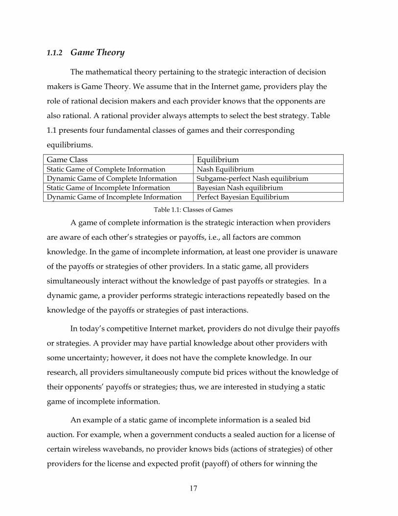
also rational. A rational provider always attempts to select the best strategy. Table
1.1 presents four fundamental classes of games and their corresponding
equilibriums.
Game Class Equilibrium Static Game of Complete Information Nash Equilibrium Dynamic Game of Complete Information Subgame-perfect Nash equilibrium Static Game of Incomplete Information Bayesian Nash equilibrium Dynamic Game of Incomplete Information Perfect Bayesian Equilibrium
Table 1.1: Classes of Games
A game of complete information is the strategic interaction when providers
are aware of each other’s strategies or payoffs, i.e., all factors are common
knowledge. In the game of incomplete information, at least one provider is unaware
of the payoffs or strategies of other providers. In a static game, all providers
simultaneously interact without the knowledge of past payoffs or strategies. In a
dynamic game, a provider performs strategic interactions repeatedly based on the
knowledge of the payoffs or strategies of past interactions.
In today’s competitive Internet market, providers do not divulge their payoffs
or strategies. A provider may have partial knowledge about other providers with
some uncertainty; however, it does not have the complete knowledge. In our
research, all providers simultaneously compute bid prices without the knowledge of
their opponents’ payoffs or strategies; thus, we are interested in studying a static
game of incomplete information.
An example of a static game of incomplete information is a sealed bid
auction. For example, when a government conducts a sealed auction for a license of
certain wireless wavebands, no provider knows bids (actions of strategies) of other
providers for the license and expected profit (payoff) of others for winning the
18
license. All the providers submit simultaneous sealed bids. Mathematics refers to
this strategic interaction as the Bayesian static game of incomplete information
because it uses Bayes’ conditional probability rule.
1.1.2.1 Bayesian Static Game of Incomplete Information
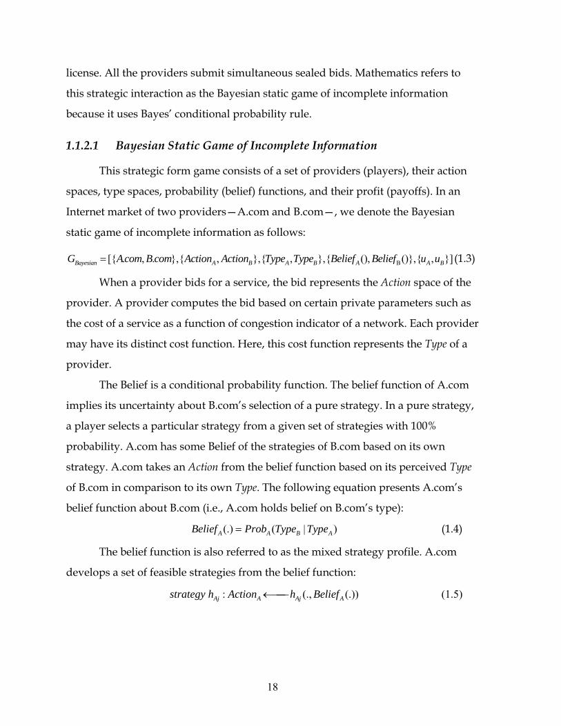
This strategic form game consists of a set of providers (players), their action
spaces, type spaces, probability (belief) functions, and their profit (payoffs). In an
Internet market of two providers—A.com and B.com—, we denote the Bayesian
static game of incomplete information as follows:
B[ . , . , , , , , (), (), , ]Bayesian A B A B A A BG Acom B com Action Action Type Type Belief Belief u u= (1.3)
When a provider bids for a service, the bid represents the Action space of the
provider. A provider computes the bid based on certain private parameters such as
the cost of a service as a function of congestion indicator of a network. Each provider
may have its distinct cost function. Here, this cost function represents the Type of a
provider.
The Belief is a conditional probability function. The belief function of A.com
implies its uncertainty about B.com’s selection of a pure strategy. In a pure strategy,
a player selects a particular strategy from a given set of strategies with 100%
probability. A.com has some Belief of the strategies of B.com based on its own
strategy. A.com takes an Action from the belief function based on its perceived Type
of B.com in comparison to its own Type. The following equation presents A.com’s
belief function about B.com (i.e., A.com holds belief on B.com’s type):
(.) ( | )A A B ABelief Prob Type Type= (1.4)
The belief function is also referred to as the mixed strategy profile. A.com
develops a set of feasible strategies from the belief function:
: (., (.))Aj A Aj Astrategy h Action h Belief←⎯⎯ (1.5)
19
For example, from a service cost function (TypeA), A.com develops a belief
(BeliefA) function for the possible bids of B.com; then, A.com selects a bid (Action) by
a strategy (h) such that A.com bid is higher than the perceived bids of B.com.
The development of the providers’ belief functions and the selection of the
best strategy set from the belief function to maximize providers’ profit (payoffs) in
the dynamic Internet traffic demand are the principal tasks of our research.
1.1.2.2 Bayesian Nash Equilibrium
A Bayesian Nash equilibrium is a feasible strategy set that maximizes
providers’ expected profit (u(.)) in a static game of incomplete information. This
equilibrium occurs when A.com and B.com play their best strategies ( * *,A Bh h ) and
results in a set of optimum expected profit ( * *[ ], [ ])A BE u E u . In the following definition,
A.com plays the best strategy in response to the best strategy played by B.com.
Definition: A strategy set 1 2( , ,..., )jStrategy h h h= constitutes a Bayesian Nash
Equilibrium of a game [ . , . , , , , ]A B A BG A com B com Strategy Strategy u u= for every
feasible strategy (j) such that:
* * *[ ( , )] [ ( , )]jA Aj Bj A Aj BjE u h h E u h h∀≥ (1.6)
Here, when B.com plays the optimal strategy *Bjh , A.com has nothing to
improve its expected profit by changing strategy from *Ajh . This also implies that
when A.com plays the optimal strategy *Ajh , B.com has nothing to improve its
expected profit by changing strategy from *Bjh .
* * *[ ( , )] [ ( , )]jB Aj Bj B Aj BjE u h h E u h h∀≥ (1.7)
Therefore, neither A.com nor B.com will benefit in expected profit by
changing strategies from the Bayesian-Nash equilibrium strategies.
20
1.1.3 Oligopoly
An Internet oligopoly market consists of a small number of providers that
strategically interact to optimize their profit. They collectively influence the network
capacity of the market and the market price of services; however, no single provider
can completely control the market. In this thesis, A.com and B.com constitute a two
provider oligopoly; i.e., duopoly.
There are two fundamental models of oligopoly: the Cournot game of
capacity and the Bertrand game of price. In today’s competitive Internet market,
providers first implement network infrastructure at the peering interface and then
assign a price. The Bertrand game of price occurs in the short term; but in the long
term, the providers reassign capacity engaging in Cournot’s game of capacity. Our
study focuses on the short-term market when market capacity remains constant and
the providers engage in price bidding. Therefore, we develop a novel model based
on the Bertrand game of oligopoly (see details in Chapter 3).
1.1.4 Sealed Bid Reverse Auction
The sealed bid reverse auction is the foundation of the price transaction
protocol of the novel model. In this auction, a buyer has a maximum price it is
willing to pay for a service. This price is the reservation price. The buyer informs
providers the reservation price of the service and seeks bids. Privately, providers
compute the prices of service and report their prices of service in sealed bids to the
buyer.
21
1.2 Background Research on Network Pricing
There is a wide range of methods used to find an optimum policy of pricing
for Internet services. Summaries of the pricing research can be found in
[9],[26],[27],[28],[29],[30],[31],[32]. The following examples are central to our
research.
1.2.1 Service per Customers’ Bids
In a pioneering study of a pricing model where customers send bids to a
provider for a service, Kelly [7] addresses the issues of charging, rate control, and
routing for a network that carries elastic—variable rate--traffic. He proposes a
market where each customer submits a bid to the provider. In Kelly’s research, the
bid is the willingness to pay per unit of time. The provider accepts these submitted
bids and determines the price of each network link. Then the provider assigns the
user a data-rate in proportion to his bid. The rate is inversely proportional to the
price of the links the customer wishes to use. The study does not employ game
theory because customers do not anticipate the effect of their actions on the prices of
the links. Nevertheless, the study shows that such a scheme maximizes the profit.
1.2.2 Static Congestion Game
Johari and Tsitsiklis [8] explore the properties of a static game where users of
a congested resource anticipate the effect of their actions on the price of the resource.
In their study, a single network allocates network capacity among a collection of
users. Each user applies a profit function depending on their allocated rates. The
profit function depends on the total rate obtained from the network. The
optimization of max-flow problems yields the rate. The network supports
homogeneous traffic, i.e. only one class of service. The market model is similar to
Kelly [7] except that users anticipate the effects of their actions simultaneously.
Thus, the model becomes a static game. Johari’s network game uses individual bids
22
at each link, as opposed to Kelly's game where each user submits a single bid to the
network.
Johari’s et al.’s study shows that for a single provider, the users receive a
Nash equilibrium profit of at least ¾ of the maximum possible aggregate profit. The
results also show that the self-interested behavior of the individual user does not
create congestion or degrade performance if a pricing mechanism is carefully
chosen. In our research, we use congestion as a parameter of network cost.
1.2.3 Provider’s Monopolist Game
DaSilva [9] espouses a game theory approach when studying static pricing
policies for multi-service networks. He conducts the study in ATM1 networks of
priority-based and allocation-based weighted round robin (WRR) scheduling. The
study uses a non-cooperative game among a set of users where a provider
determines a price in advance. The provider strategy is to optimize the operating
point of the network by adjusting the price. A user strategy is to maximize its profit
given all other users’ service choices. Here, the provider is a monopolist and the
users are the players. A provider induces one or more Nash equilibriums according
to the network architecture, the available resources, and the pricing policy adopted.
The study demonstrates that the adoption of an appropriate pricing policy enables
the service provider to offer the necessary incentives for each user to choose the
service that best matches its needs, thereby discouraging over-allocation of resources
and maximizing customer’s profit. Richard La et al. [10] study a similar monopoly
market. In contrast, we study an oligopoly market.
1 Asynchronous Transfer Mode (ATM) network supports cells or fixed sized packets
23
1.2.4 Peer Providers in a Series
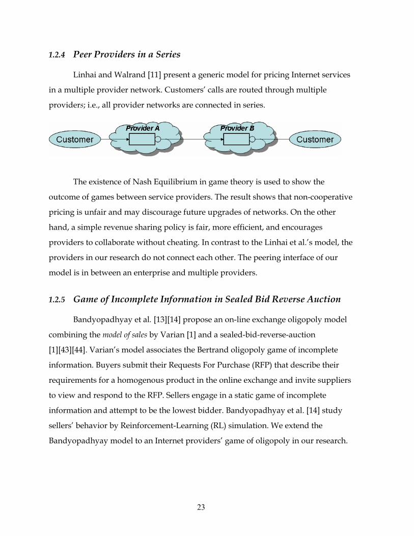
Linhai and Walrand [11] present a generic model for pricing Internet services
in a multiple provider network. Customers’ calls are routed through multiple
providers; i.e., all provider networks are connected in series.
The existence of Nash Equilibrium in game theory is used to show the
outcome of games between service providers. The result shows that non-cooperative
pricing is unfair and may discourage future upgrades of networks. On the other
hand, a simple revenue sharing policy is fair, more efficient, and encourages
providers to collaborate without cheating. In contrast to the Linhai et al.’s model, the
providers in our research do not connect each other. The peering interface of our
model is in between an enterprise and multiple providers.
1.2.5 Game of Incomplete Information in Sealed Bid Reverse Auction
Bandyopadhyay et al. [13][14] propose an on-line exchange oligopoly model
combining the model of sales by Varian [1] and a sealed-bid-reverse-auction
[1][43][44]. Varian’s model associates the Bertrand oligopoly game of incomplete
information. Buyers submit their Requests For Purchase (RFP) that describe their
requirements for a homogenous product in the online exchange and invite suppliers
to view and respond to the RFP. Sellers engage in a static game of incomplete
information and attempt to be the lowest bidder. Bandyopadhyay et al. [14] study
sellers’ behavior by Reinforcement-Learning (RL) simulation. We extend the
Bandyopadhyay model to an Internet providers’ game of oligopoly in our research.
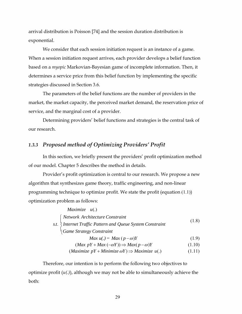
Selecting a strategically appropriate price is our method to optimize revenue.
We will provide a best strategy selection method that determines appropriate price
from the belief function of the providers’ oligopoly game.
Change in traffic pattern varies the degree of congestion in the network. A
key indicator of network congestion is the mean packet count in the network’s
queue systems. An increase in the packet count in the system increases the mean
delay in packet transmission. Consequently, it degrades the service quality. The
degradation of service is detrimental to revenue. Thus, our model associates the
network congestion with the service cost.
The mean packet count in the queue system of each provider varies with the
change in the traffic load of its network and the routing pattern of traffic inside the
network. Enforcing optimal routing [85] to minimize network congestion—the mean
packet count in the queue system—is our method of minimizing service cost. We
apply two well-known non-linear programming techniques, the Gradient Projection
and the Golden Section Line search methods [46][48][49] [50], to minimize the mean
packet count in the system.
Each network node of this research is equipped with an infinite memory
single integrated output queue per link using the First-In-First-Out (FIFO)
scheduling scheme. We assume that the IP packet arrival process and the packet size
distributions, respectfully, are Poisson and Exponential. When traffic aggregates into
a queue, the aggregate traffic arrival process and packet length distributions are
Poisson and Hyper-Exponential. Thus, we assume the well-known classical
Markovian (M) General model (M/G/1)[74][75] of queuing theory. Thus, we
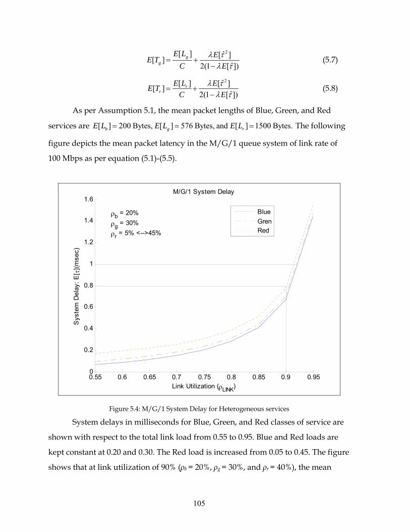
perform M/G/1 queuing analysis [74] to develop traffic-engineering rules.
However, we approximate the mean packet count in the queue system using
31
M/M/1 theory so that we may use results from the theory of M/M/1 network
queue systems.
1.3.4 Proposed Algorithm
Our algorithm for a session or a game instance to optimize provider profit
consists of the following steps:
i) Enforce traffic engineering rules based on M/G/1;
ii) Perform optimum traffic routing;
iii) Approximate the optimum congestion indicator (mean packet count2
in the network based on M/M/1);
iv) Develop instantaneous congestion-sensitive service cost;
v) Develop the belief function by the proposed game of oligopoly;
vi) Select the best strategy to determine strategically appropriate price;
vii) Conduct game: simulation of session initiations-terminations and
emulate customer price negotiation by sealed bid reverse auction
protocol.
1.3.5 Research Methods
We conduct mathematical analyses and simulation to evaluate the
performance of the Automatic Price Transaction-based One-to-Many Peer Network
architecture that implements the Providers’ Optimized Game in Internet Traffic model.
Our research methods consist of the followings:
• Develop the Automatic Price Transaction-based One-to-Many Peer Network
architecture and associated protocols for a two providers SIP based
network.
2 The literature [85] develops optimum routing as a function of optimum mean delay. On the other hand, we develop optimum routing as a function of optimum mean packet count because majority of the vendor routers keep the record of mean packet count instead of mean delay. We want to stress that there is no difference in the mean delay method and our mean packet count method because they are directly related through Little’s Law [59],[60].
32
• Develop the Providers’ Optimized Game in Internet Traffic model:
o Develop a duopoly market, define parameters of the belief
function, develop analytical model of the belief function, and
identify a set of strategies.
o Develop the non-linear program to perform optimal routing [85].
o Design a network, develop traffic engineer rules, and assign traffic
paths.
• Develop a simulation model in the MATLAB3 tool.
We verify analytical models by simulation results. By maintaining the
simulated market demand equal to the mathematical desired demand, we compare
the simulated market price and the simulated provider profit with corresponding
values from analysis. We determine the best strategy (the Bayesian-Nash
equilibrium and Pareto-efficient outcome) to optimize provider market shares of
profit in all market demand for the homogenous and heterogeneous classes of
service. Chapter 7 and 8 describe details of these methods.
3 MATLAB ) is an integrated technical and mathematical computing tool and is a product of MathWorks (www.mathworks.com).
33
1.4 Distinguishing Characteristic of our approach
In our approach, customers have options for subscribing to services from a
provider of choice based on the price using the new Automatic Price Transaction-based
One-to-Many Peer Network architecture. In addition, we propose a method for
providers to optimize profit using the new game model, the Providers Optimized
Game in Internet Traffic. This game model is sensitive to the dynamic Internet traffic
demand, the congestion in networks and the service class.
The Third Generation Partnership Project (3GPP) develops wireless standards
that refer to pricing as charging. The recent work [69]-[73] in 3GPP on charging uses
a wireless consumer to provider (one-to-one) model. However, it does not provide
options for customers to negotiate price with providers in one-to-many peer
architecture similar to our architecture.
SIP based peering among multiple providers is a new phenomenon. The
ATIS-PTSC4 is developing SIP based IP peering standards between two providers
for one-to-one peer network [68]. However, the ATIS initiative lacks automatic
pricing mechanism and one-to-many peer features.
The Internet Engineering Task Force (IETF) is an Internet professional
community that develops Internet protocol specifications known as Request For
Comment (RFC). The IETF RFC 3455 [67] specifies SIP header fields to transport
price information; however, it does not provide any example of SIP flow to
implement price transaction. We provide an example of SIP flow to illustrate the
price transaction method.
Lin et al.’ [15] research is an example of a transaction-based pricing, which
can be viewed as the automatic pricing between an enterprise and a provider.
However, they do not provide solutions for enterprise-provider one-to-many peer
networks. 4 The Alliance for Telecommunications Industry Solutions (ATIS) is a North American standard organization. Packet Technologies and Systems Committee (PTSC) is an ATIS committee that develops standards related to Internet services, architectures, and signaling.
34
Significant Internet services pricing research [9][10][11][17][18][21][23][26]
relates monopoly markets where consumers strategically interacts to get services
from a single provider The study of an oligopoly market where providers are
competing for enterprises is the main distinguishing characteristic of our research.
The majority of the literature on pricing [9][26][27][28][29][30[[31][32] does
not provide any price transaction protocol or algorithm to compute price. In this
dissertation, we suggest an automatic price transaction protocol, a SIP flow, and an
algorithm to compute price.
Although academics conducted significant research on dynamic pricing in the
1990s, critics pointed out that the computational complexity would make the
dynamic pricing expensive and hard to implement [9]. The recent significant
technological advance in microprocessors and memory enables networks to perform
complex computations on per session and per packet basis. Therefore, dynamic
pricing schemes will not be hard to implement. In addition, the fall in the price of
microprocessors will also make it inexpensive. Criticism against the dynamic pricing
is no longer valid as the technology advances and becomes affordable. It is
particularly true for the Voice over IP (VoIP). More importantly, our dynamic
pricing scheme is not between a consumer and a provider; rather, it is at the peering
interface between provider and enterprise to transport aggregate traffic.
Another common criticism [9] of dynamic pricing is that the customers may
have to pay more than their budget if the price fluctuates; as a result, a dynamic
pricing scheme will encounter adverse reaction from them. Our proposed dynamic
pricing mechanism deploys a sealed bid reverse auction. In this mechanism,
enterprises send their fixed budget value as a reservation price to the providers and
the providers always bid less than the customers’ budgeted amount.
While we propose a dynamic pricing mechanism, we implement a static
game. As mentioned earlier, our model stems from the Bandyopadhyay et al.
[13][14] and Varian’s [1] static game of incomplete information. In our model, the
commodity is the internet bandwidth rate per class of service whereas in
35
Bandyopadhyay et al.’s model the commodities are goods (e.g. auto-parts) sold in an
on-line exchange. The Bandyopadhyay et al. oligopoly model assumes a symmetric
market—the market demand and marginal cost do not change during the game.
Internet traffic demand and network congestion dynamically change depending
upon the time of the day, day of the week, and special days of the year. Thus, static
market demand and static marginal cost do not map well with the provider game of
oligopoly. We take into account the dynamic nature of Internet traffic demand and
congestion in the network; thus, we study an asymmetric market.
The Bandyopadhyay et al. model is a two-step static game. A firm sells its
total capacity at once, and then another firm sells the total residual demand. In our
model, each SIP-based session setup is an event of a game and the bandwidth for
each session is much less than the market capacity. The sessions are established as
well as deactivated according to the arrival load. One of the parameters of the game
uses a one-step near-sighted history for each session arrival game. Thus, our model
is a “myopic” Markovian game. In addition, a market consists of regional markets
that have capacity restrictions. We study both the homogeneous and the
heterogeneous service-based networks.
In [14], the Reinforcement Learning (RL) procedure by simulation is proposed
for determining the best strategy from the mixed strategy equilibrium. The RL is
suitable when marginal cost is constant. Due to the dynamic nature of the Internet,
converging to a best strategy with RL will be difficult to achieve. The
implementation of the RL mechanism in the network device may also add extra cost.
Therefore, we simplify the implementation by defining a set of feasible strategies
from the mixed strategy equilibrium. Then, we identify the best strategy from this
set by analytical and simulation methods.
36
1.5 Summary of Contribution
The major contributions of our research are as follows:
• We proposed the Automatic Price Transaction-based One-to-Many Peer Network
architecture allows providers and customers to automatically negotiate price.
It facilitates customers’ options for subscribing services from a provider that
offers the lowest price. This proposed architecture introduces a new service in
the Internet and the wireless market.
• The proposed architecture extends the ATIS one-to-one peer and the 3GPP
charging architectures to support one-to-many peer model.
• We propose a price transaction protocol and a SIP flow for the proposed
architecture.
• Proposed Providers Optimized Game in Internet Traffic model allows providers to
offer competitive service price within the budget of the customers. The model
eliminates the reactive time of price computation. The model is sensitive to
the dynamic internet traffic demand, the network congestion cost, and the
service class.
• We propose an algorithm to implement the game model synthesizing game
theory, traffic engineering technique and non-linear programming.
• We develop a simulation tool implementing the proposed algorithm.
• Our method determines the dominant, the Bayesian-Nash equilibrium, and
the Pareto-efficient outcome strategies from a set of feasible strategies. These
strategies maximize providers’ expected profit.
• Our method achieves relative advantage over the classical Bertrand model of
price, which is commonly used in the short-term market.
• Our method decreases the market price of services relative to the customers’
budgets while guaranteeing customers’ preferences.
• Our method optimizes profit in fair market share and in fair market
throughput.
37
• In addition to the profit optimization, providers can implement our method
to perform least price routing, traffic load distribution, capacity planning, and
service provisioning.
1.6 Structure of the Dissertation
In Chapter 2, we present the Automatic Price Transaction-based One-to-Many
Peer Network architecture and associated price-transaction protocol, and the SIP call
flow. Chapter 3 develops providers’ game of oligopoly by defining parameters and
stating assumptions. A method of defining a feasible strategy set is presented. We
develop a non-linear program in Chapter 4 to optimize traffic flow in the network to
minimize the mean packet count in the network queue system. This traffic flow
optimization minimizes the marginal cost of service and maximizes provider profit.
In Chapter 5, we present the research design of a duopoly network architecture,
assigning the capacity of links and describing traffic flow through the network.
Chapter 6 presents the algorithm of the Providers Optimized Game in Internet Traffic
model and the simulation algorithm. In Chapter 7, we perform mathematical
analyses and validation. In Chapter 8, we present simulation results and model
applications for homogeneous and heterogeneous service-based networks. We
conclude with lessons learned and possible future directions of this research in
Chapter 9. We provide two appendices: In Appendix A, we outline mathematical
optimization techniques; in Appendix B, we present acronyms.
38
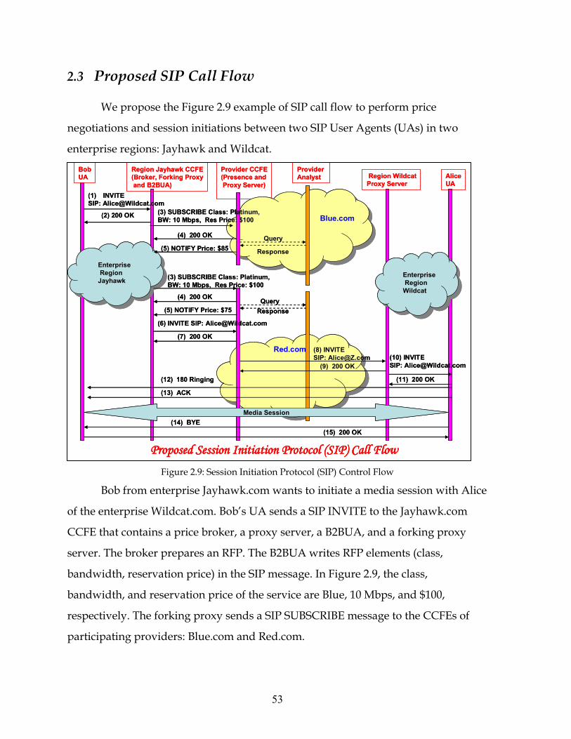
2 Network Architecture and Protocol
This chapter describes the new Automatic Price Transaction-based One-to-Many
Peer Network architecture where customers peer with providers by Session Initiation
Protocol (SIP) based intelligent entities at the interconnect interfaces. These SIP
entities automatically perform price negotiations, session management, policy and
security enforcements, and service delivery assurance. This chapter focuses on the
price-based network architectures, price negotiation techniques, and the SIP
protocol.
2.1 Network Architecture
In this section, we first present outlines of SIP entities. Second, we briefly
describe the general Internet Protocol (IP) peering network architecture of Alliance
for Telecommunications Industry Standards (ATIS)5 and 3GPP charging
architecture. Then, we propose our price-based network architecture and protocol.
Finally, we present a SIP flow.
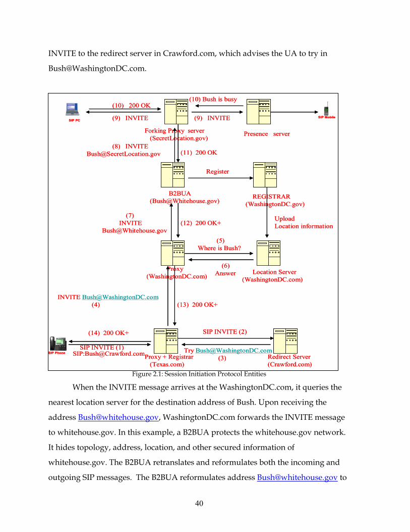
2.1.1 SIP Entities
SIP is a signaling protocol to create, modify, and terminate multimedia
sessions in the Internet. IETF Request For Comment (RFC) 3261 [66] describes the
foundation of SIP. Other RFCs define SIP extensions to deliver signals for IP based
multimedia applications. SIP is a nascent protocol and continued development of
SIP standards and applications are underway. A detailed description of SIP can
found in SIP related IETF RFCs6 and literatures [61]-[65]. The main entities of SIP are
User Agents (UA), registrars, proxy servers, location server, redirect servers, and
presence servers.
5 ATIS standards can be viewed at http://www.atis.org 6 SIP RFCs can be viewed at SIP, SIPPING, SIMPLE, and MMUSIC working groups of IETF (www.ietf.org).
39
UAs reside in users’ applications such as phones, computers, video
equipment, Personal Digital Assistants (PDAs). This equipment can be either mobile
or fixed. A UA initiates and establishes voice or multi-media sessions with another
UA. When a UA is connected to the network, it first registers its location with the
SIP network entity called a registrar.
Proxy servers are SIP routers. Generally, a proxy and a registrar are located in
the same physical box. The function of a registrar is to keep the location addresses of
the users. A proxy learns the location address of the destination from the nearest
registrar and routes a SIP message towards the destination addresses. In case a
registrar does not reside in the same box as a proxy, the proxy seeks the destination
address from a location server, which contains a database of current locations of
each user.
A proxy server can forward a SIP message to either a single destination or
multiple destinations. A proxy server capable of forwarding SIP messages to
multiple destinations is called a forking proxy. A redirect server does not route a SIP
message but provides the potential address of the destination to the UA that sends
the SIP message. Note that we do not show many other SIP messages in this
example.
A Back-to-Back User Agent (B2BUA) is the combination of two user agents or
proxies into the same entity. It breaks an end-to-end session to multiple call legs. It
terminates a session then reformulates and re-originates the session. This enforces
security and policy to a SIP session.
A presence server provides information about reachability, availability,
consent, and user profiles. The ongoing projects at IETF and in the research
community are adding innovative features in the presence server.
We illustrate a hypothetical scenario in Figure 2-1. A high school buddy from
Crawford, Texas wishes to speak to President Bush. When he dials Bush’s phone
number, a SIP INVITE message is sent from the UA of his phone to the proxy and
the registrar in Texas.com, which cannot locate Bush. Therefore, it forwards the
40
INVITE to the redirect server in Crawford.com, which advises the UA to try in
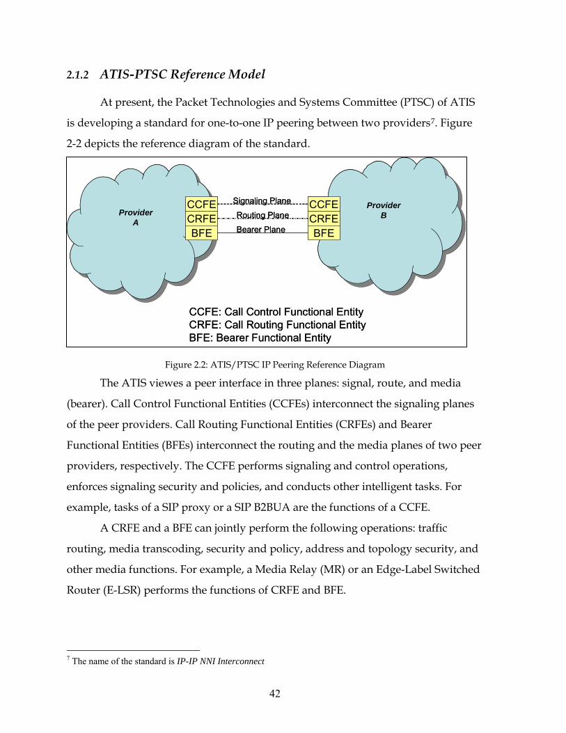
In the ATIS-PTSC one-to-one peer architecture, an enterprise interconnects
with only one provider. We propose a one-to-many peer architecture that allows an
enterprise to peer with multiple providers. Each enterprise can maintain physical
connections to all providers in the market. The enterprise configures separate and
parallel Label Switch Paths (LSPs) to all the providers. The LSPs are elastic, i.e. the
bandwidth of the data path through the providers may vary. This enables each
enterprise to either transmit all of its traffic through one provider or distribute its
traffic to all providers. LSPs are configured through the BFEs of the enterprise and
providers. Note that the providers are not connected with each other.
We propose two new modules—a price broker and a price analyst—as a part of
the peering mechanism between an enterprise and providers. An enterprise price
broker computes the reservation price of a service and develops a Request For
Purchase (RFP) data element. An analyst of a provider computes the price of service
based on the provider’s game strategies as proposed in Chapter 3.
We also propose a forking proxy server at the CCFE of the enterprise and a
combined module of a presence server and B2BUA at the CCFE of each provider.
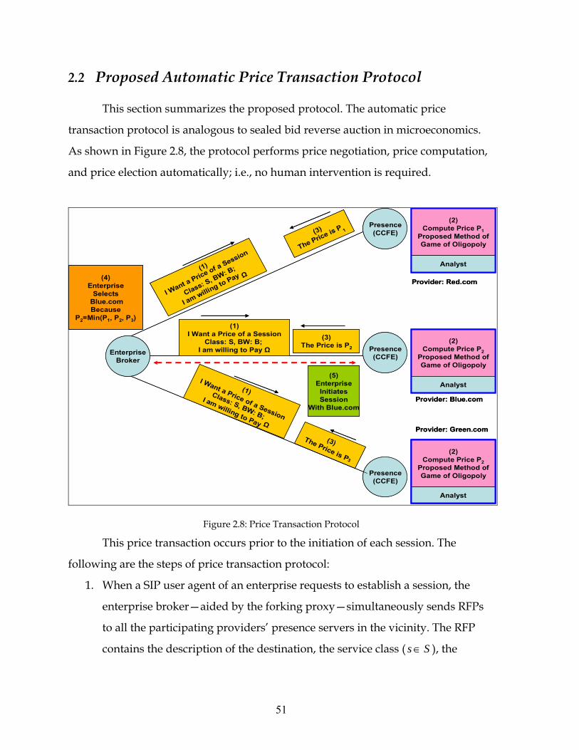
The automatic transaction protocol of Section 2.1.6 illustrates price
negotiation between an enterprise broker and a provider analyst. An enterprise
provides services to the consumers—SIP user agents—requiring separate multi-
media sessions through the provider’s network. In the enterprise network, when a
UA requests a connection, the price broker sends the RFP to the forking proxy. This
proxy transmits the RFP to all the peer providers. In a provider network, the
presence server receives the RFP from the enterprise and passes it to the price
analyst. Then, the analyst informs the presence server of the price of service. The
provider’s presence server passes the price as a bid to the enterprise proxy, which in
turn forwards it to the broker of the enterprise. After receiving all the bids from all
the providers, the broker selects the lowest priced provider and instructs the
44
enterprise proxy server to initiate the session to the destination through this
provider. Note that the enterprise assumes that all providers deliver identical QoS
for each service class. The proxy instructs the BFE to create a media path between
the enterprise and the provider to transport media over IP packets.
In a provider network, an analyst is either a central entity or distributed
entities located with the CCFEs. We assume that an analyst is a central entity in each
provider’s network. The analyst can either compute the price of a service
periodically or upon a session request. The granularity of the period will be
implementation specific and will be determined by the network designers. We
assume that the analyst computes the price of a session for each session request.
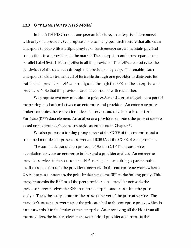
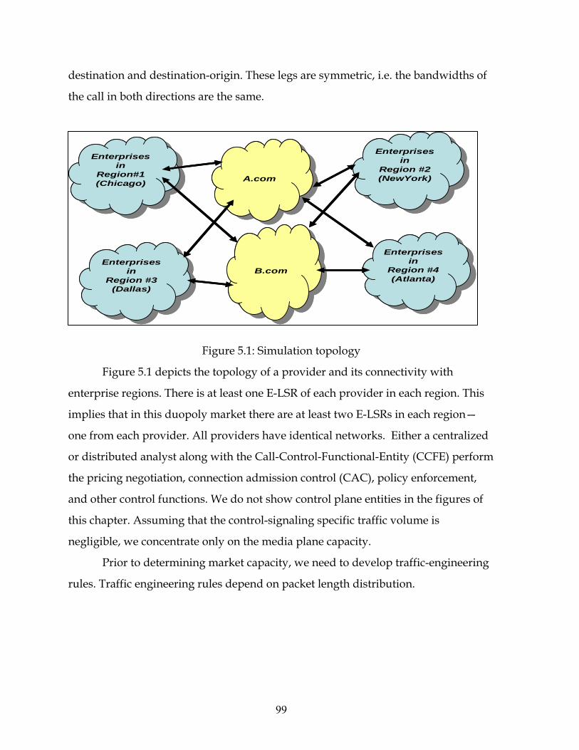
Figure 2.3: Network Architecture of Duopoly Market
Figure 2-3 depicts the proposed network architecture in a duopoly market.
There are two providers (Blue.com and Red.com) and four regions in this market.
There are multiple enterprises in each region. Each enterprise peers with both
Blue.com and Red.com. Each provider implements a centralized analyst. The price
broker resides with the CCFE of each enterprise network. E-LSRs perform the
functions of CRFEs and BFEs.
Blue.comBlue.com
Red.comRed.com
CustomerRegion#1
CustomerRegion#1
CustomerRegion#3
CustomerRegion#3
Enterprise C
CCFEE-LSR
CCFEE-LSR
CCFEE-LSR
CustomerRegion#2
CustomerRegion#2
Enterprise B
CustomerRegion#4
CustomerRegion#4
Enterprise A CCFEE-LSR
Enterprise D
CCFEE-LSR
Analyst
BrokerPresence
Analyst
CCFEE-LSR
Broker
CCFEE-LSR
Broker
CCFEE-LSR
Broker
Presence
Presence
Presence
45
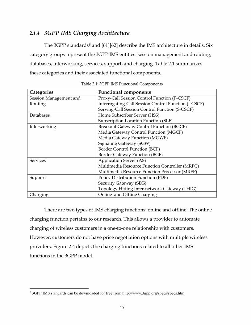
2.1.4 3GPP IMS Charging Architecture
The 3GPP standards8 and [61][62] describe the IMS architecture in details. Six
category groups represent the 3GPP IMS entities: session management and routing,
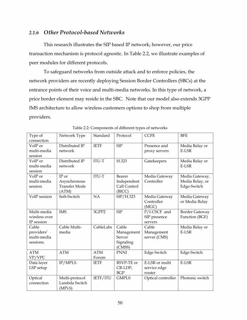
databases, interworking, services, support, and charging. Table 2.1 summarizes
these categories and their associated functional components.
Table 2.1: 3GPP IMS Functional Components
Categories Functional components Session Management and Routing
Proxy-Call Session Control Function (P-CSCF) Interrogating-Call Session Control Function (I-CSCF) Serving-Call Session Control Function (S-CSCF)
Databases Home Subscriber Server (HSS) Subscription Location Function (SLF)
Interworking Breakout Gateway Control Function (BGCF) Media Gateway Control Function (MGCF) Media Gateway Function (MGWF) Signaling Gateway (SGW) Border Control Function (BCF) Border Gateway Function (BGF)
Services Application Server (AS) Multimedia Resource Function Controller (MRFC) Multimedia Resource Function Processor (MRFP)
Support Policy Distribution Function (PDF) Security Gateway (SEG) Topology Hiding Inter-network Gateway (THIG)
Charging Online and Offline Charging
There are two types of IMS charging functions: online and offline. The online
charging function pertains to our research. This allows a provider to automate
charging of wireless customers in a one-to-one relationship with customers.
However, customers do not have price negotiation options with multiple wireless
providers. Figure 2.4 depicts the charging functions related to all other IMS
functions in the 3GPP model.
8 3GPP IMS standards can be downloaded for free from http://www.3gpp.org/specs/specs.htm
46
Figure 2.4: 3GPP IMS Architecture
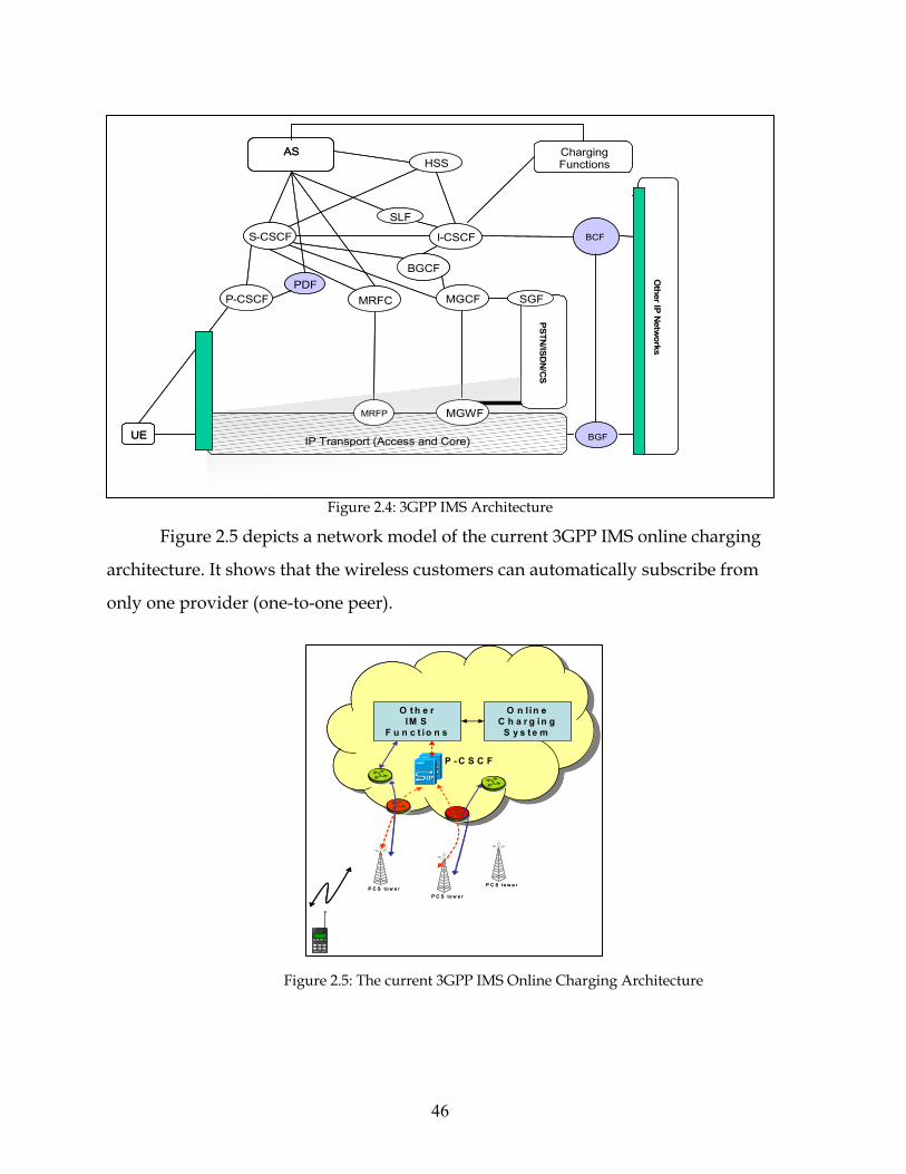
Figure 2.5 depicts a network model of the current 3GPP IMS online charging
architecture. It shows that the wireless customers can automatically subscribe from
only one provider (one-to-one peer).
Figure 2.5: The current 3GPP IMS Online Charging Architecture
P - C S C F
P C S to w e r
P C S to w e r
P C S to w e r
O t h e rIM S
F u n c t io n s
O n l in eC h a r g in g
S y s t e m
P - C S C F
P C S to w e r
P C S to w e r
P C S to w e r
O t h e rIM S
F u n c t io n s
O n l in eC h a r g in g
S y s t e m
IP Transport (Access and Core)
ChargingFunctions
AS ChargingFunctionsHSS
I-CSCF
SLF
BGCF
MGCFMRFCP-CSCF
UE
MRFP
Other IP N
etworks
BCF
PDF
PSTN/ISD
N/C
S
SGF
S-CSCF
BGF
MGWF
IP Transport (Access and Core)
ChargingFunctions
AS ChargingFunctionsHSS
I-CSCF
SLF
BGCF
MGCFMRFCP-CSCF
UE
MRFP
Other IP N
etworks
BCF
PDF
PSTN/ISD
N/C
S
SGF
S-CSCF
BGF
MGWF
47
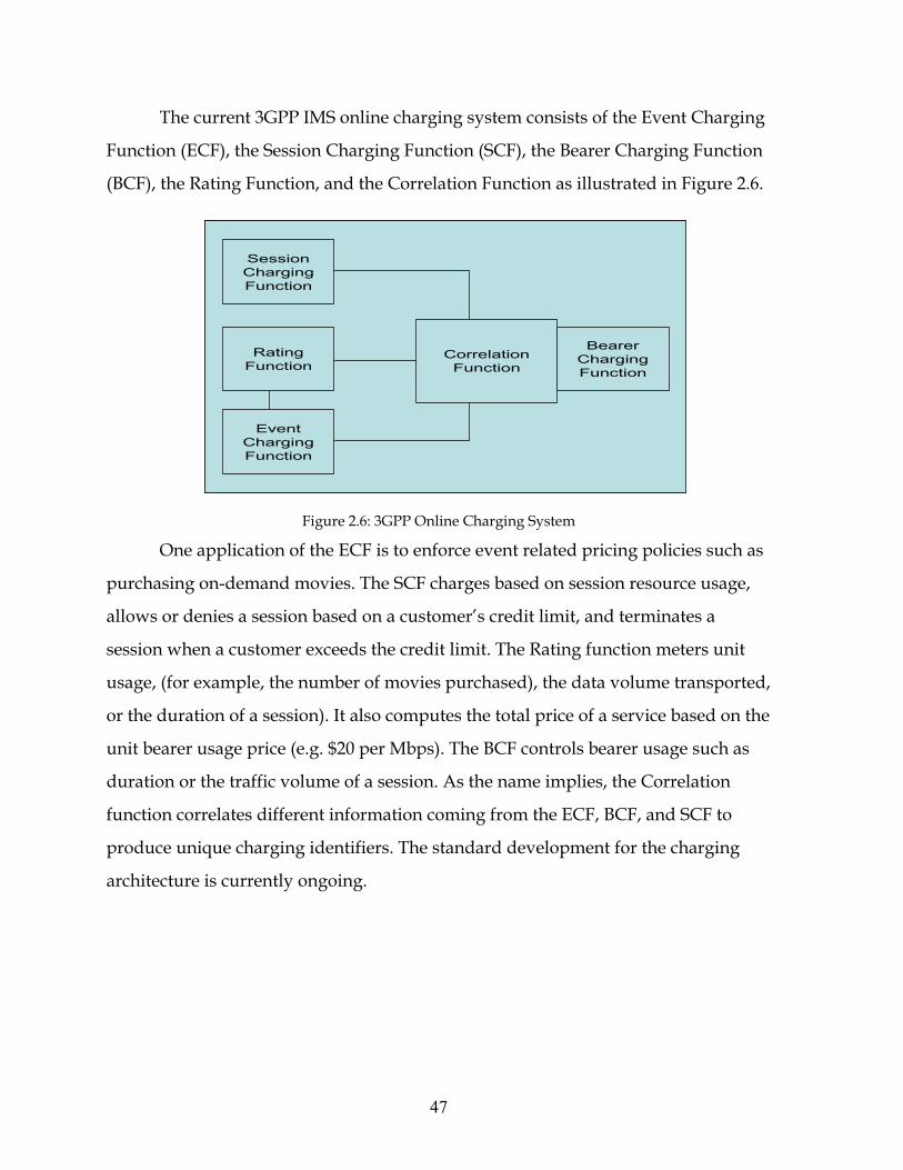
The current 3GPP IMS online charging system consists of the Event Charging
Function (ECF), the Session Charging Function (SCF), the Bearer Charging Function
(BCF), the Rating Function, and the Correlation Function as illustrated in Figure 2.6.
Figure 2.6: 3GPP Online Charging System
One application of the ECF is to enforce event related pricing policies such as
purchasing on-demand movies. The SCF charges based on session resource usage,
allows or denies a session based on a customer’s credit limit, and terminates a
session when a customer exceeds the credit limit. The Rating function meters unit
usage, (for example, the number of movies purchased), the data volume transported,
or the duration of a session). It also computes the total price of a service based on the
unit bearer usage price (e.g. $20 per Mbps). The BCF controls bearer usage such as
duration or the traffic volume of a session. As the name implies, the Correlation
function correlates different information coming from the ECF, BCF, and SCF to
produce unique charging identifiers. The standard development for the charging
architecture is currently ongoing.
SessionChargingFunction
RatingFunction
EventChargingFunction
BearerChargingFunction
CorrelationFunction
SessionChargingFunction
RatingFunction
EventChargingFunction
BearerChargingFunction
CorrelationFunction
48
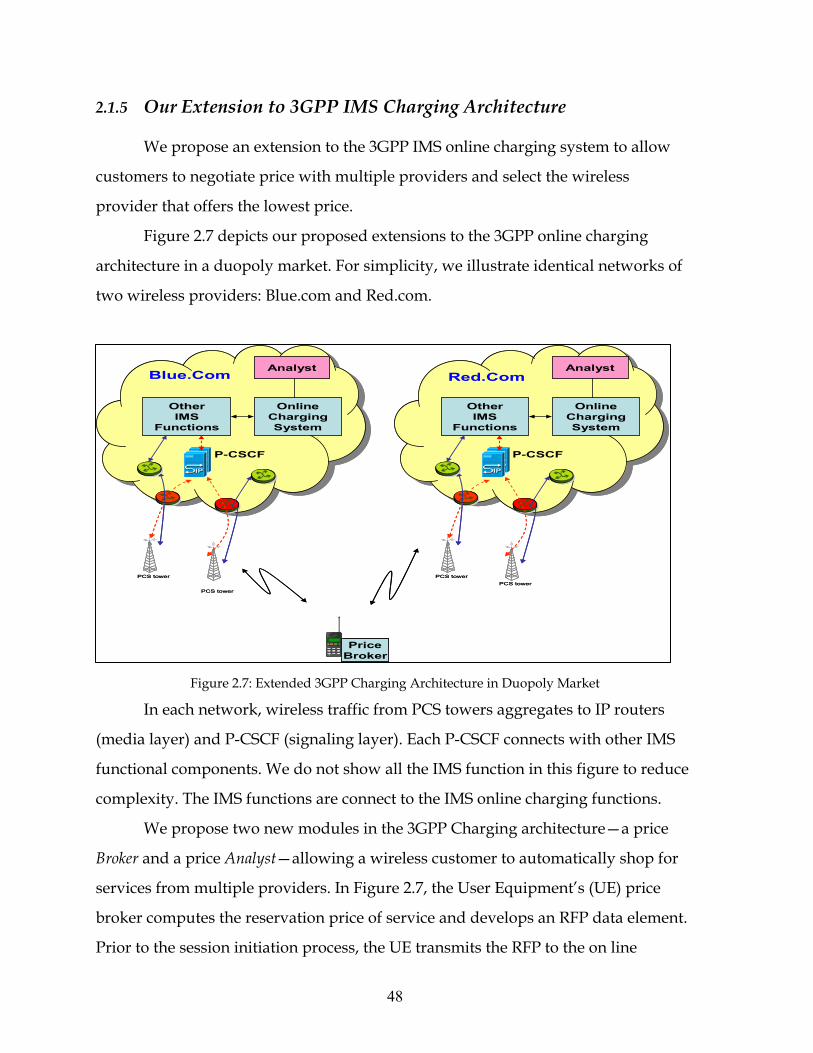
2.1.5 Our Extension to 3GPP IMS Charging Architecture
We propose an extension to the 3GPP IMS online charging system to allow
customers to negotiate price with multiple providers and select the wireless
provider that offers the lowest price.
Figure 2.7 depicts our proposed extensions to the 3GPP online charging
architecture in a duopoly market. For simplicity, we illustrate identical networks of
two wireless providers: Blue.com and Red.com.
Figure 2.7: Extended 3GPP Charging Architecture in Duopoly Market
In each network, wireless traffic from PCS towers aggregates to IP routers
(media layer) and P-CSCF (signaling layer). Each P-CSCF connects with other IMS
functional components. We do not show all the IMS function in this figure to reduce
complexity. The IMS functions are connect to the IMS online charging functions.
We propose two new modules in the 3GPP Charging architecture—a price
Broker and a price Analyst—allowing a wireless customer to automatically shop for
services from multiple providers. In Figure 2.7, the User Equipment’s (UE) price
broker computes the reservation price of service and develops an RFP data element.
Prior to the session initiation process, the UE transmits the RFP to the on line
P-CSCF
PCS towerPCS tower
OtherIMS
Functions
OnlineChargingSystem
Analyst
PriceBroker
P-CSCF
PCS tower
PCS tower
OtherIMS
Functions
OnlineChargingSystem
AnalystBlue.Com Red.Com
P-CSCF
PCS towerPCS tower
OtherIMS
Functions
OnlineChargingSystem
Analyst
PriceBroker
P-CSCF
PCS tower
PCS tower
OtherIMS
Functions
OnlineChargingSystem
AnalystBlue.Com Red.Com
49
charging module of a provider via P-CSCF and other IMS modules. The analyst
connects with the online charging module. An analyst of a wireless provider
computes the unit bearer usage price of service based on the provider’s game
strategies as proposed in Chapter 3.
Price negotiation between a UE’s broker and a provider’s analyst is analogous
to the automatic transaction protocol of Section 2.1.6. The UE transmits the RFP to
all the wireless providers. In each network, the P-CSCF receives the RFP and passes
it to the price analyst. Then, the analyst feeds the unit bearer usage price of service
to the Rating function. The online charging system computes the appropriate price.
Using the provider’s wireless equipment and SIP, the provider’s P-CSCF passes the
price as a bid to the customer’s broker. After receiving all the bids from the
providers, the broker selects the lowest priced provider and instructs the SIP user
agent of the wireless UE to initiate the session with this provider.
Our pricing model for both ATIS and 3GPP are analogous. Therefore, in the
rest of this thesis, we will concentrate on only one: the proposed one-to-many
enterprise-provider peer architecture (extension of the ATIS model) as described in
Section 2.1.3.
50
2.1.6 Other Protocol-based Networks
This research illustrates the SIP based IP network; however, our price
transaction mechanism is protocol agnostic. In Table 2.2, we illustrate examples of
peer modules for different protocols.
To safeguard networks from outside attack and to enforce policies, the
network providers are recently deploying Session Border Controllers (SBCs) at the
entrance points of their voice and multi-media networks. In this type of network, a
price border element may reside in the SBC. Note that our model also extends 3GPP
IMS architecture to allow wireless customers options to shop from multiple
providers.
Table 2.2: Components of different types of networks
Type of connection
Network Type Standard Protocol CCFE BFE
VoIP or multi-media session
Distributed IP network
IETF SIP Presence and proxy servers
Media Relay or E-LSR
VoIP or multi-media session
Distributed IP network
ITU-T H.323 Gatekeepers Media Relay or E-LSR
VoIP or multi-media session
IP or Asynchronous Transfer Mode (ATM)
ITU-T Bearer Independent Call Control (BICC)
Media Gateway Controller
Media Gateway, Media Relay, or Edge-Switch
VoIP session Soft-Switch NA SIP/H.323 Media Gateway Controller (MGC)
Media Gateway or Media Relay
Multi-media wireless over IP session
IMS
3GPP2 SIP P/I-CSCF and SIP presence servers
Border Gateway Function (BGF)
Cable providers’ multi-media sessions.
Cable Multi-media
CableLabs
Cable Management Server Signaling (CMSS)
Cable Management server (CMS)
Media Relay or E-LSR
ATM VP/VPC
ATM ATM Forum
PNNI Edge Switch Edge Switch
Data layer LSP setup
IP/MPLS IETF RSVP-TE or CR-LDP, BGP
E-LSR or multi service edge router
E-LSR
Optical connection
Multi-protocol Lambda Switch (MPλS)
IETF/ITU GMPLS Optical controller Photonic switch
51
2.2 Proposed Automatic Price Transaction Protocol
This section summarizes the proposed protocol. The automatic price
transaction protocol is analogous to sealed bid reverse auction in microeconomics.
As shown in Figure 2.8, the protocol performs price negotiation, price computation,
and price election automatically; i.e., no human intervention is required.
EnterpriseBroker
Presence(CCFE)
Presence(CCFE)
Presence(CCFE)
(1)
I Want a Price of a Session
Class: S, BW: B;
I am willing to Pay Ω
(1)I Want a Price of a Session
Class: S, BW: B;
I am willing to Pay Ω
(1)I Want a Price of a Session
Class: S, BW: B; I am willing to Pay Ω
(2)Compute Price P1
Proposed Method ofGame of Oligopoly
(3)
The Price is P 1
(3)The Price is P2
(3)The Price is P3
(4)Enterprise
SelectsBlue.comBecause
P2=Min(P1, P2, P3)
(5)Enterprise
InitiatesSession
With Blue.com
Analyst
(2)Compute Price P2
Proposed Method ofGame of Oligopoly
Analyst
(2)Compute Price P2
Proposed Method ofGame of Oligopoly
Analyst
Provider: Red.com
Provider: Blue.com
Provider: Green.com
EnterpriseBroker
Presence(CCFE)
Presence(CCFE)
Presence(CCFE)
(1)
I Want a Price of a Session
Class: S, BW: B;
I am willing to Pay Ω
(1)I Want a Price of a Session
Class: S, BW: B;
I am willing to Pay Ω
(1)I Want a Price of a Session
Class: S, BW: B; I am willing to Pay Ω
(2)Compute Price P1
Proposed Method ofGame of Oligopoly
(3)
The Price is P 1
(3)The Price is P2
(3)The Price is P3
(4)Enterprise
SelectsBlue.comBecause
P2=Min(P1, P2, P3)
(5)Enterprise
InitiatesSession
With Blue.com
Analyst
(2)Compute Price P2
Proposed Method ofGame of Oligopoly
Analyst
(2)Compute Price P2
Proposed Method ofGame of Oligopoly
Analyst
(2)Compute Price P2
Proposed Method ofGame of Oligopoly
Analyst
Provider: Red.com
Provider: Blue.com
Provider: Green.com
Figure 2.8: Price Transaction Protocol
This price transaction occurs prior to the initiation of each session. The
following are the steps of price transaction protocol:
1. When a SIP user agent of an enterprise requests to establish a session, the
enterprise broker—aided by the forking proxy—simultaneously sends RFPs
to all the participating providers’ presence servers in the vicinity. The RFP
contains the description of the destination, the service class ( Ss∈ ), the
52
enterprise index (i), the session bandwidth (B), and the service reservation
price ( siΩ ).
2. The providers’ presence servers query their respective analysts to learn the
price of the requested service. Analysts of all the providers compute the price
of the service based on their own game strategies.
3. Presence servers of providers notify the enterprise broker of their bids for the
session.
4. After receiving all the bids ( Pp∈ ), the broker of the enterprise selects the
lowest priced provider and instructs its peer element to initiate the session.
5. The enterprise peer element sends a SIP INVITE message to the proxy of the
winning provider.
53
2.3 Proposed SIP Call Flow
We propose the Figure 2.9 example of SIP call flow to perform price
negotiations and session initiations between two SIP User Agents (UAs) in two
enterprise regions: Jayhawk and Wildcat.
Figure 2.9: Session Initiation Protocol (SIP) Control Flow
Bob from enterprise Jayhawk.com wants to initiate a media session with Alice
of the enterprise Wildcat.com. Bob’s UA sends a SIP INVITE to the Jayhawk.com
CCFE that contains a price broker, a proxy server, a B2BUA, and a forking proxy
server. The broker prepares an RFP. The B2BUA writes RFP elements (class,
bandwidth, reservation price) in the SIP message. In Figure 2.9, the class,
bandwidth, and reservation price of the service are Blue, 10 Mbps, and $100,
respectively. The forking proxy sends a SIP SUBSCRIBE message to the CCFEs of
participating providers: Blue.com and Red.com.
BobUA
Region Jayhawk CCFE(Broker, Forking Proxyand B2BUA)
We extend Varian’s and Bandyopadhyay et al.’s models to allow for the
varying nature of marginal cost and perceived market demand of the Internet. The
mixed strategy profile of our model is a function of fixed market capacity, the
perceived time varying market demand function, the time varying marginal cost
function, and the customers’ fixed reservation price of services. This makes our
model asymmetric.
59
3.2 Service Class and Enterprise Preference
The commodity of this market is bandwidth. All the sessions in this research
have equal bandwidth. The type of value that a provider adds to a session identifies
a class of service. To meet the diverse application needs of an enterprise, providers
have to furnish different types of services based on the technology and network
intelligence used. For example, different applications offered by enterprises may
require different levels of security guarantees, types of addressing schemes (e.g.
IPv4 vs. IPv6), and types of digital signal processing.
We develop service class based on customers’ preference, i.e., how customers
value each service. However, the distinguishing value does not relate QoS
parameters such as delay performance. All class of service must adhere to a
required delay performance. Customers value services based on their preferences
such as security treatement, encryption, protection from packet dropping, etc.
Exactly what the value is not important—all that matters is that customers are
willing to pay different amounts for the different services.
Assumption: Enterprises request three groups of services based upon their
required security levels: High, Medium, and Low.
Assumption: Each provider in a heterogeneous service-based market offers
three classes of service called Blue, Green, and Red. These three classes guarantee
customers’ required security levels of High, Medium, and Low, respectively.
Assumption: Each provider in a homogeneous service-based market offers a
single class of service (Green) that guarantees Medium level security.
Assumption: Enterprises prefer that providers guarantee security levels.
We assume that the commodity space (S) is represented by the Internet
service bandwidth with the desired security levels High, Medium, Low and every
enterprise prefers that providers guarantee these security levels. The consumption
60
bundles b, g, and r in the commodity space (S) are mapped, respectively, to Blue,
Green, and Red.
, ,b g r S∈ (3.2)
We expand the preference definitions of [1] for our proposed class of services.
By denoting the enterprise strict preference as “ ”, the term , ,b g S b g∈ implies
that an enterprise strictly prefers the security level guaranteed by the Blue service to
that of the Green service. Enterprises in this market satisfy the following important
properties:
Complete: For b, g ∈ S, either b g or g b . In our model, the security level
of the Blue service is strictly preferred over that of Green service; however, the
reverse is not true.
Reflexive: For g ∈ S, g g . For the homogeneous based-service (i.e. when
only the Green service is available in the market), the security level of all sessions
should be Green (i.e. medium).
Transitive: For b, g, r ∈ S, if b g and g r , then b r . Blue security level
is strictly preferred over Green, and Green security level is strictly preferred over
Red. It is also true that the security level of the Blue service is strictly preferred to
that of the Red service. This property is important because the market price for Blue
service (pb) will be higher than the market price for Green service (pg) and the
market price of Green service (pg) will be higher than that of Red(pr).
b g rp p p> > (3.3)
Enterprises will also be willing to a pay higher price for Blue over Green and
Green over Red. Due to the transitive property, the relation among their reservation
prices will be as follows:
b g rΩ > Ω > Ω (3.4)
61
Continuity: For b, g ∈ S, the sets :s b g= and :s g b= are closed sets
and :s b g and :s g b are open sets. In our model, since higher security levels
are strictly preferred to the lower security levels, they constitute an open set. In this
research, this open set or strict preference property is important because the cost of
providing two different levels of security is not the same. In Section 3.3.2, we
develop a cost function of providers based on the service cost coefficient for
different classes.
Assumption: Different levels of security require a different cost to provide a
service. Thus, the costs of producing different classes of service are different.
In this research, service class does not depend on the performance parameter
because all classes of traffic share integrated queues in each link and FIFO non-
preemptive priority scheduling serves the link. Note also that provider networks in
this study implement Call Admission Control (CAC) and enforce traffic-engineering
rules to guarantee Quality of Service (See Section 5.3).
As per [1], the profit function (U: X → R) quantifies the preference
comparison of an enterprise. The fact that the profit enjoyed by the highly secured
Blue service is greater than the profit enjoyed by the moderately secured Green
services implies that enterprises strictly desire the Blue service over the Green
service. The following represents this relation between enterprise’s profit and
preference:
( ) ( )U b U g b g⇔ (3.5)
We do not study the profit of the enterprise. Nevertheless, we reflect
customer profit by three levels of reservation price as presented in Section 3.3.3.
62
3.3 Model Parameters
3.3.1 Market Capacity and Market Demand Functions
In this section, we present definitions and assumptions concerning the market
capacity and market demand of our proposed model.
Definition: Market capacity (Γ) is the aggregate traffic engineered access
bandwidth capacities of all providers in a market. Market capacity is a fixed
quantity measured in bandwidth rate per unit time (e.g. Mbps). It is the sum of the
capacity of all the access ports of Edge-Label Switched Routers (E-LSRs) or media-
relays of all the providers in a market multiplied by the Maximum Traffic
Engineered Link Load9 ( TEρ ). By denoting nK as the total capacity of all the access
ports of a provider (n), the following equation represents the market capacity.
1 1
N N
n TE TE nn n
K Kρ ρ= =
Γ = =∑ ∑ (3.6)
Assumption: A provider market capacity is finite.
Definition: Market demand (Δ) is the aggregate bandwidth requested by all
the enterprises in a market. Market demand is a variable quantity measured in
bandwidth rate per unit (e.g. Mbps). The maximum market demand is denoted by
Δmax.
MaxΔ ≤ Δ (3.7)
Assumption: Maximum Market Demand (ΔMax) is less than the market
capacity (Γ).
MaxΔ < Γ (3.8)
Assumption: Every provider’s market capacity is less than the market
demand.
TE nK nρ < Δ ∀ (3.9)
9 Providers limit load of a network below a maximum limit during capacity planning and traffic engineering to maintain delay jitter level in the node. We define this limit as Traffic Engineered bandwidth capacity and the load as Maximum Traffic Engineered Load.
63
Assumption: Market demand is greater than (N-1) times a provider’s market
capacity if there are N numbers of providers in the market. The relation between
market demand and capacity can be written as follows:
( 1)TE nN K nρ − < Δ ∀ (3.10)
To understand equation (3.10), let us assume that there are four providers in a
market. Here, market demand is such that if three providers sell to their market
capacity, then the remaining provider sells to a fraction of its market capacity when
it sells to the residual demand. Note, equation (3.10) subsumes equation (3.9).
The equations (3.7)-(3.10) can be written as follows:
( 1)TE n MaxN K nρ − < Δ ≤ Δ < Γ ∀ (3.11)
Definition: The throughput ( nY ) of a provider is the total outgoing traffic
from the provider in all regions.
In our study, market demand is a variable quantity. Each provider has
knowledge of its throughput level ( ,n tY ) at time t. From this knowledge, each
provider develops its perceived market demand function.
Assumption: The provider networks are lossless (no packet drop or session
drop occurs).
Assumption: Each provider perceives that the market maintains fair shares of
bandwidth among the providers.
Definition: The perceived market demand (Δ ) of a provider is the
multiplication of its production level with the number of providers in the market.
We express the perceived market demand function by the following equation.
, ,( )n t n tY NYΔ = (3.12)
Based on the above assumptions and definitions, we define the market
demand as a function of ,n tY .
Definition: If perceived market demand is less than the market capacity of a
provider, the market demand is the lower bound of equation (3.11); otherwise, the
64
market demand is equivalent to the perceived demand. The market demand
function is depicted by Figure 3-1 and represented by the following equation:
,,
, ,
( 1) , 0( ) TE n t TE
n tn t TE n t Max
N K NY KY
NY K NYρ ε ρ ε
ρ− + ≤ >⎧
Δ = ⎨ < ≤ Δ⎩ (3.13)
The top portion of equation (3.13) is to satisfy equation (3.10). The bottom
portion of equation (3.13) implies the provider’s perception that a fair market share
is achieved at the steady state operating load.
Figure 3.1: Demand Function
3.3.2 Marginal Cost Function
In this section, we define cost and marginal cost functions. Cost to provide a
service depends on many parameters and network situations.
Assumption: There is no cost associated with the distance.
Rationale: Prior to the explosive growth of the Internet, the expensive Public
Switched Telephone Network’s (PSTN) price of service was a function of the
distance traveled (e.g. long-distance or international) by a call. Massive deployment
Δ(Y)
YNρK
(N-1)ρK
(N-1)ρK
Γ = NρK
ΔMax
N = 2
Δ
ΔMax
Δ(Y) = NY
Δ(Y) = (N-1)ρK + ε
Δ(Y)
YNρK
(N-1)ρK
(N-1)ρK
Γ = NρK
ΔMax
N = 2
Δ
ΔMax
Δ(Y) = NY
Δ(Y) = (N-1)ρK + ε
65
of fiber-optic cables around the globe reduced the distance specific cost for Internet
services. At present, ISPs do not charge based on distance.
We assume the following four influences on the service cost:
1. Congestion in the network
2. Protocol used to provide a service (service class discriminator)
3. Amount of service (commodity)
4. Providers’ fixed cost to produce the service
Assumption: The service cost is a function of the congestion indicator in the
network, i.e. the optimum mean packet count in the queue system in the network.
Rationale: Congestion in the network increases the delay in packet
transmission. The delay degrades the service quality. The degradation of service is
detrimental to the revenue because it will be reasonable for providers to pay the
enterprise a penalty for delay violation. The mean packet count in the queue system
is a congestion indicator of the network. Congestion in the network varies with
time. By performing optimum routing, the congestion in a network can be well
distributed across the network; as a result, the network can support more traffic
compared to a non-optimized network. The efficient routing yields the optimum
mean packet count in the network queue system.
Assumption: The service cost is a function of the service cost coefficient.
Rationale: The class is differentiated by the service cost coefficient parameter.
The service cost coefficient parameter depends on the protocol and intelligence
applied to provide the service. For example, to guarantee levels of security requires
different network costs. As mentioned earlier, the service cost coefficient of service
class is not differentiated by the performance parameter because all classes of traffic
share integrated queues in each link and is serviced by FIFO non-preemptive
priority scheduling.
Assumption: Each provider maintains the identical QoS for all class.
Assumption: The service cost coefficient of a class is the same for all the
providers.
66
Rationale: The service cost coefficient of a class will either be the same for all
the providers or be different for different providers. In reality, providers purchase
equipment and software from the same set of vendors. Therefore, the service cost
coefficient of an identical class for different provider is generally the same.
Assumption: The cost of a service is a function of a provider’s fixed cost.
Rationale: Different providers assign different costs to deploy and maintain
the service.
From the above assumptions, we can assert the following:
Assertion: The service cost is a function of the service cost-coefficient ( sδ ), the
mean packet count in the queue system ( ˆnM ), throughput (Yn), and the provider
fixed cost coefficient (θ n).
, , , , , , ,ˆ( ) ( )n s t n t n t s n t n t n n tCost Y g Y M Y Yδ θ= = + (3.14)
Note that the service cost is computed for bandwidth per unit of time.
Therefore, call duration is not considered in equation (3.14). The mean packet count
in a network varies with the change in the throughput of the network, i.e. Mn,t is a
function of Yn,t.
, ,( )n t n tf Y M→ (3.15)
In microeconomics, the marginal cost is defined as the change in cost
( (.)Cost∂ ) due to the change in production or output ( Y∂ ).
The marginal cost = (.)CostY
∂∂
(3.16)
Definition: Marginal service cost is the increase in cost for adding another
unit amount of bandwidth in the network.
Based on the above definition and equations (3.14)-(3.16), the marginal cost
function of a service class for a provider is represented as follows. (Note, cost is a
continuous function of Y).
, ,, , , , ,
, ,
ˆ( )ˆ ˆ( ) ( )n t n tn s t n t s n t n t n
n t n t
g Y MM Y M
Y Yω δ θ
∂ ∂= = + +
∂ ∂ (3.17)
67
The above equation denotes the marginal cost of a service as a function of the
service cost coefficient, provider fixed cost coefficient, and change in the mean
packet count of each provider with respect to the change in throughput. The service
cost coefficient and the provider fixed cost jointly enforce a differentiated price per
class and per provider.
Since at each instant of time, each provider has a distinct mean packet count,
the marginal cost of two providers may not be identical at any instant of time.
Besides, fixed cost coefficient (θ n) of each provider is unique. Therefore, marginal
cost will be different for different providers even if the mean packet count is the
same.
Table 3.1 illustrates a sample representation of marginal cost equations for
different providers in heterogeneous service networks supporting Blue, Green, and
Red classes of service. Section 7.2 presents the rationale for selecting the following
service cost coefficient values.
Table 3.1: Marginal cost equation
Blue Green Red Provider 1
*1, *
1, 1,1,
ˆˆ1.00( ) 10t
t tt
MY M
Y∂
+ +∂
*1, *
1, 1,1,
ˆˆ0.10( ) 10t
t tt
MY M
Y∂
+ +∂
*1, *
1, 1,1,
ˆˆ0.01( ) 10t
t tt
MY M
Y∂
+ +∂
Provider 2
*2, *
2, 2,2,
ˆˆ1.00( ) 10t
t tt
MY M
Y∂
+ +∂
*2, *
2, 2,2,
ˆˆ0.10( ) 10t
t tt
MY M
Y∂
+ +∂
*2, *
2, 2,2,
ˆˆ0.01( ) 10t
t tt
MY M
Y∂
+ +∂
3.3.3 Reservation Price of an Enterprise
Not only is the reservation price of a service (i.e., the maximum price) that an
enterprise is willing to pay for a unit of each service, it is also the upper bound of the
enterprise budget. Reservation prices are determined during the business agreement
and remain constant throughout the lifetime of the game. Enterprises are rational
agents and they do not violate the agreement by changing the reservation price. For
homogeneous services, the reservation price is a fixed value for all enterprises. For
68
the heterogeneous services (Blue, Green, and Red), there are three fixed reservation
prices.
We explained the following relation between the enterprise profit and
preference in Section 3.2:
( ) ( )U b U g b g⇔ (3.18)
Due to the relation of equation (3.18), an enterprise will be willing to pay a
higher price for Blue service over Green service and Green service over Red service.
Because of this relation and the transitive property of preference, the relation among
their reservation prices will be as follows:
b g rΩ > Ω > Ω (3.19)
How does an enterprise broker compute its maximum bid price or the
reservation price (Ωs) for a service? Enterprises may adopt many different methods
to compute the maximum reservation price for their services. Providers may not
dictate the method of computing reservation prices to enterprises. However, we
suggest that enterprises assume monopoly market while determining the price of
service. Here, we do not study the method of determining the reservation price.
Assumption: The bandwidth required for each session is the same.
Assumption: The reservation prices do not change during the game.
Assumption: The reservation prices are always greater than all providers’
marginal costs, i.e. s sωΩ > Computation of a reservation price can be a future research topic. For
example, a study on the influence of varied reservation price on providers’ profit
would be useful to observe whether enterprises can control the market power of the
providers.
69
3.3.4 Profit Function
Profit obtained from time T0 to Tend, while maintaining upper bound of
throughput (Y), can be described as follows.
0 0
( (.)) ( ( , ) ( , ))endT Y
TU p p t y t y dydtω= −∫ ∫ (3.20)
In the proposed network architecture, a session occurs at each instance of a
game. A session initiation event can be either a Set-Up Request or Tear-Down
Request. For each session set-up request, if the CAC of a provider can admit the call,
the provider computes the bid price and the enterprise activates the session through
the winning provider network. Since the bandwidth of each session is much smaller
than a providers’ market capacity, and since calls activate and de-activate, the
winning provider continues to take part in the game for subsequent session
initiation requests. The steady state operating point (network throughput) of a
provider is achieved when the provider’s price stabilizes with the competitive
market price. If two providers are competing in a market and they adopt different
cost functions, their steady state operating point (network throughput) can be
different although both of them will operate at the same competitive market price.
We will examine this by session level Monte-Carlo simulation in Chapter 8.
Figure 3.2: The Sketch of Steady State Price, Cost, Throughput, and Profit
Price (p(.))
Marginal Cost (ω(.))
Network Throughput (Y)
Profit ( u(.))
dt dt
dt dt
Unit-Profit
Price (p(.))
Time (t)
Marginal Cost (ω(.))
Network Throughput (Y)
(.))
dt dt
dt dt
-
Mar
ket P
rice
M
argi
nal C
ost
Thro
ughp
ut
Prof
it
Time (t)
Time (t)
Time (t)
Price (p(.))
Marginal Cost (ω(.))
Network Throughput (Y)
Profit ( u(.))
dt dt
dt dt
Unit-Profit
Price (p(.))
Time (t)
Marginal Cost (ω(.))
Network Throughput (Y)
(.))
dt dt
dt dt
-
Mar
ket P
rice
M
argi
nal C
ost
Thro
ughp
ut
Prof
it
Time (t)
Time (t)
Time (t)
70
Figure 3.2 provides a sketch of the market price, network throughput,
marginal cost, and providers’ profit to explain our unit profit function. The figure
illustrates that in a steady state, marginal cost and network throughput do not
significantly vary for a unit duration of time (dt). As a result, the price of service also
remains stable. The provider’s profit per unit time will be the product of the steady
state throughput and the difference between steady state unit price and marginal
cost. For example, in a steady state, if a bid price is $90 per Mbps, a marginal cost is
$50 per Mbps, and a steady state operating point throughput is 300 Mbps, then the
unit profit obtained is $12,000.
Definition: The unit profit of a provider is the profit per unit duration (e.g.
one second) measured at an instant of the steady state throughput ( Y ) when the bid
price and the marginal cost of the provider converge to p and ω .
ˆˆˆ( ) ( )u p p Yω= − (3.21)
A provider (n) computes profit from a session as a function of the price (p),
the marginal cost (ω), the duration (d), and the bandwidth (y) of the session. The
price and the marginal cost are values at the session start time. The total profit of the
provider is the sum of the profits from all ( k∀ ) the sessions until the end of the
game (e.g. a session-level Monte-Carlo simulation).
, , , , , , , ,( )n s t k n s t k n k n s kk
Cumulative profit p d yω∀
= −∑ (3.22)
71
3.4 Proposed Oligopoly Model
This section derives our game of oligopoly model based on Varian’s and
Bandyopadhyay et al.’s models described in section 3.1. These two models extend
the Bertrand oligopoly model to the static game of incomplete information. The
static Bayesian game [1]-[5] represents the static game of incomplete information.
As described in Chapter 1, a static Bayesian game consists of Action space,
Type space, Strategy space (mixed strategy profile or belief function), and Payoff
space. In this research, we propose that the static Bayesian game consists of the
following elements:
• Strategic players: providers (N).
• Action space: the bids of the providers (pbid).
• Type space: the marginal cost function of the providers (ω(.)).
• Strategy space: the set of functions over mixed strategy profile or belief
function F(.). This is a price randomizing cumulative probability
distribution function.
• Payoff space: the expected unit profit (u(.)) of the providers at the steady
state.
The commodity of the market is bandwidth (y) and the strategic variable is
the price (p) of Internet services (s). In this game, the strategy of a provider is to
maximize expected profit.
By applying Varian’s and Bandyopadhyay et al.’s methods of developing F(p)
and our assumptions in this chapter, we develop F(p) for an Internet duopoly
market.
Assumption: The price randomizing cumulative probability distributive
function F(p) is a continuous function and the associated probability distribution
function is f(p). Each provider implements the same method to develop F(p).
72
Assumption: The providers compete in an asymmetric equilibrium market,
i.e. each provider determines a price from the different F(p).
Definition: The minimum price (pMin) is a price that allows a provider to win
a bid with 100% probability.
Definition: The mixed strategy profile of a provider, b( ) (p )F p Prob p= ≤ ,
represents the opponents’ probability of selecting bid (pb) less than or equal to a
price p, where [ , ]b Minp p p∈ . This definition also implies that if a provider bids a
price p, then its opponents will win the bid with a probability of b(p )Prob p≤ .
Assumption: If both providers bid the same price (a tie), enterprises select a
provider at random (uniform distribution); i.e. enterprises select with 50%
probability. However, the probability of a tie is negligible.
We define a bid as the price per rate per class of service. Consider in a market
with two providers: A.com and B.com. Denote F(p) as the mixed strategy profile of
A.com. If A.com bids with a price p from F(p) and B.com bids with any other price
pb, then two possible scenarios occur.
• Scenario 1: A’s price is lower than B’s price: bp p> .
• Scenario 2: A’s price is higher than or equal to B’s price: bp p≤ .
73
Scenario 1: A.com’s price (p) is lower than B.com’s price ( B bidp ): B bidp p>
o This event (Scenario 1) occurs with a probability equal to
1 ( ) ( )bF p Prob p p− = > which is 0.2 in the above figure.
o Since p is the lower bid, A.com wins. Consequently, p becomes the
market price at that instant.
o Denote the unit profit obtained at this price by A.com as ( )Lu p and the
profit obtained in a long duration of time is (from time T1 to T2) as UL(p)
o At the steady state operating point, if the bid price of A.com is lower, it
will sell to its market capacity. Thus, it will operate on maximum market
capacity throughput.
o At the steady state, price and marginal cost do not significantly vary.
Since this price is lower than that of B.com, A.com sells to the market
capacity at this steady state ( ˆTEY Kρ= ). If the game occurs for a unit
duration of time, the unit profit obtained at this price by A.com can be
represented by the following equation:
ˆ( ) ( (.)) ( (.))L TEu p p Y p Kω ω ρ= − = − (3.23)
o By selecting the lowest price pMin, A.com can sell to its market capacity
with 100% probability; thus, it can obtain unit profit as follows:
( ) ( (.))L Min Min TEu p p Kω ρ= − (3.24)
Price (p)
F(p)
1.0
0.8
0.5
0.2
Mixed Strategy Profile of A
pMin p
pb
If A Bids here
If B Bids here
Price (p)
F(p)
1.0
0.8
0.5
0.2
Mixed Strategy Profile of A
pMin p
pb
If A Bids here
If B Bids here
74
Scenario 2: A.com’s price is higher (p) than B.com’s price ( Bp ): Bp p≤
o This event (Scenario 2) occurs with a probability of ( ) ( )bF p Prob p p= ≤
which is 0.8 in the above figure.
o Since pb is the lower price, B.com wins.
o At the steady state operating point, if the bid price of A.com is higher, it
will sell to the residual market demand. Thus, at a steady state, it will
operate on a throughput of the residual market demand ( (.) TE KρΔ − ).
o Denote the profit obtained at this price by A.com as ( )Hu p .
o The unit profit obtained at this price by A.com in the steady state is
represented by the following equation:
( ) ( (.))( (.) )H TEu p p Kω ρ= − Δ − (3.25)
o If a provider’s strategy were to maximize its expected unit profit by
having a high price strategy, it would rather select a reservation price. In
this case, the unit profit function of A.com appears as follows:
( ) ( (.))( (.) )H TEu Kω ρΩ = Ω− Δ − (3.26)
From the above two scenarios, the expected unit profit ( ( )u p ) of A.com at the
steady state can be expressed as follows:
Price (p)
F(p)
1.0
0.8
0.5
0.2
Mixed Strategy Profile of A
pMin p
pb
If A Bids here
If B Bids here
Price (p)
F(p)
1.0
0.8
0.5
0.2
Mixed Strategy Profile of A
pMin p
pb
If A Bids here
If B Bids here
75
( ) ( )(1 ( )) ( ) ( )L Hu p u p F p u p F p= − + (3.27)
From equation (3.27), we can derive the mixed strategy profile:
( ) ( )( )( ) ( )L
L H
u p u pF pu p u p
−=
− (3.28)
Assumption: The probability that a provider bids a price less than or equal to
the reservation price is 1; i.e. F(Ω) = 1.
Since F(p) = 1 at price p = Ω, equation (3.27) yields the following:
( ) ( )Hu p u= Ω (3.29)
By substituting equations (3.24)-(3.29) in (3.27), the mixed strategy profile of
A.com can be developed as follows:
( (.)) ( (.))( (.) )( )( (.))(2 (.))
TE TE
TE
p K KF pp K
ω ρ ω ρω ρ
− − Ω− Δ −=
− −Δ (3.30)
Following the above approach, we can derive the mixed strategy profile for N
providers when a provider plans to bid either highest or lowest. Now A.com is
competing with N-1 providers. The probability of A.com’s winning the bid is 1( ( ))NF p − if its bid is the highest and the probability of winning the bid is
( 11 ( ( ))NF p −− if its bid is the lowest. The steady state expected unit profit is as
follows:
1 1
1
( ) ( )(1 ( ( )) ) ( )( ( ))
( ) ( )( )( ) ( )
N NL H
N
L
L H
u p u p F p u p F p
u p u pF pu p u p
− −
−
= − +
⎡ ⎤−=> = ⎢ ⎥−⎣ ⎦
(3.31)
By having the lowest bid among the providers, A.com can sell to its market
capacity obtaining the following steady state unit profit:
( ) ( (.))L TEu p p Kω ρ= − (3.32)
If A.com’s bid is the highest, it obtains the following steady unit profit by
selling the residual bandwidth ( (.) ( 1)TE N KρΔ − − ).
( ) ( (.))( (.) ( 1) ))H TEu p p N Kω ρ= − Δ − − (3.33)
76
In this case, to maximize profit, A.com’s strategy will be to select the highest
price (i.e.,Ω ).
( ) ( (.))( (.) ( 1) ))H TEu N Kω ρΩ = Ω− Δ − − (3.34)
From equations (3.29), (3.31)-(3.34), the following belief function of A.com is
derived: 1
1( (.)) ( (.))( (.) ( 1) )( )( (.))( (.))
NTE TE
TE
p K N KF pp N K
ω ρ ω ρω ρ
−⎡ ⎤− − Ω− Δ − −= ⎢ ⎥− − Δ⎣ ⎦
(3.35)
In Section 3.3, we defined the marginal cost as a function of optimized mean
packet count in the network queue system and the market demand as a function of
network throughput. Based on these definitions, we postulate the following
equation from equation (3.35) for the game time (t): 1
* * * 1, , , , , , , , ,
, , , , * *, , , , , ,
( ( )) ( ( )( ( ) ( 1) ))( )
( ( ))( ( ))
Nn s t n s t n t TE s n s t n t n t TE
n s t n s tn s t n s t n t TE n t
p M K M Y N KF p
p M N K Yω ρ ω ρ
ω ρ
−⎡ ⎤− − Ω − Δ − −= ⎢ ⎥
− −Δ⎢ ⎥⎣ ⎦(3.36)
If A.com plans to bid such that its bid price is higher than 1N providers and
less than 2N providers in an N providers’ market, A.com can approximately develop
the belief function from the following equation using our above method:
1 12 1( ) (1 ( ( )) ( ( ))1 1
N NL H
N Nu p u F p u F pN N
− −= − +− −
(3.37)
Since our research focuses on a duopoly market, where a provider will bid
either highest or lowest. Thus, we will not develop the belief function using
equation (3.37).
Equation (3.36) is a cumulative distribution function of a provider’s
probability of losing a bid because its opponents’ bids are lower. In other words, the
function , , , ,( )n s t n s tF p represents the probability that the other providers will win the
bid if A.com selects a price (p) at a game time (t) for the service class (s). This also
implies that the bid prices ( , ,other s tp ) selected by the other providers are lower than
A.com price , ,A s tp with a probability of , , , , , ,( ) ( )A s t other s t A s tF p Prob p p= ≤ .
77
The function , , ( )n s tF p is the belief function of this game of incomplete
information because it addresses the conditional probability that the other providers
will not bid a price lower than (p) with a probability (1 – , , ( )n s tF p ) if a provider (n) is
to win the bid.
Our game is a static game—it does not keep or rely on the total history. In
each game instance, the game computes the change in cost from one game instance
to the next game instance. Since the game looks into a one-step history and forgets all
other history, the strategic interaction corresponds to a “myopic” Markovian-
Bayesian [4] static game of incomplete information. The dynamic game—that relies
on the total history is outside the scope of this research and is a future research
topic.
3.5 The Movement of the Belief Function
For each session initiation request, providers compute a new belief
function, , , ( )n s tF p , to determine a bid. As discussed earlier, the belief function’s
parameters are market capacity and demand, marginal cost, and reservation price.
The marginal cost of service is a function of the optimized mean packet count in the
network, and the cost coefficients of a provider. The service cost coefficient values
are unique for each class and for different providers. The demand function varies
with an increase in throughput. The belief function , , ( )n s tF p of a service varies with
the marginal cost of a provider and the market demand. For all these reasons,
the , , ( )n s tF p per service is not identical for all the providers at a certain instant of
time. For three services, each provider supports three belief functions. Moreover, for
two provider networks, there are total of six belief functions.
78
86 88 90 92 94 96 98 100-0.2
0
0.2
0.4
0.6
0.8
1
1.2
Price (p)
Pric
e S
trate
gy, c
df, F
(p)
Capacity of each NSP = 60, Total Customer Demand = 110
* NSP1: Strategy: min(p:p-->F(p))
-- NSP2: Strategy: mean(p:p-->F(p)
Figure 3.3: Change in Belief Function due to the change in Marginal cost
Figure 3.3 illustrates how a change in marginal cost shifts the belief function
in a homogeneous service duopoly market. Both the providers have identical
networks and use identical cost functions. The belief functions, , , ( )n s tF p , are drawn
for different marginal costs. The increase in marginal cost shifts a belief function to
the right; thus, increases the price of a product. This figure is a hypothetical
representation for illustration purpose and does not represent a result of the study.
79
3.6 Providers’ Strategies
A provider’s strategy is to maximize its expected profit by selecting a price
using the belief function. The strategy space is the set of functions over the belief
function , , ( )n s tF p . This section specifies a strategy space over the belief function to
select bids in the game. In our study, each provider adopts its own strategies to
determine bid ( , ,n s tp ) using the belief function , , ( )n s tF p .
In Section 1.1.2.1, we described the following equation to represent A.com’s a
set of feasible strategies from the belief function in a Bayesian Game of Incomplete
Information:
: (., ( ))Aj A Aj B Astrategy h Action h Belief Type←⎯⎯ (3.38)
Since in our study, the action space is the bid ( , ,n s tp ) of a provider, we can
rewrite the above equation as follows:
, , , ,: ( (.))bidAj A s t Aj A s tstrategy h p h F←⎯⎯ (3.39)
A provider computes a bid from , , ( )n s tF p using certain rejection probability of
winning the bid. We map this rejection probability with provider’s strategy.
Definition: The Rejection Coefficient (γ ) of a provider is the probability of
having its bid rejected. The rejection probability of selecting a price my bidp is
( ) ( )my bid othersbid my bidF p Prob p p γ= ≤ = .
Definition: A Winning coefficient (ξ ) is the probability of winning a bid.
Definition: A No Rejection Strategy of a provider is the strategy when the
probability (γ ) of having the bid rejected is zero. In other words, in this strategy the
probability of winning a bid is 100%. Here, the winning coefficient is 1.0ξ = . In this
case, the following equation is true.
, , , ,( ) 0n s t Min s tF p γ= = (3.40)
By substituting Equation (3.40) in Equation (3.36) and performing algebra, the
following No Rejection Strategy price is developed:
80
*
, , , , *, , , , , ,
( ( ))( ( ) ( 1) )( )s n s t n t n t
Min n s t n s t n tTE
M Y N Cp M
Kω
ωρ
Ω − Δ − −= + (3.41)
Definition: An Absolute Rejection Strategy of a provider is the strategy when
the probability (γ ) of losing the bid to the opponents is almost 100%. In other words,
in this strategy having the bid rejected is almost 100%. Here, the winning coefficient is
0.0ξ = .
, , _ , , ,( ) 1.0n s t absolute risk n s tF p γ= = (3.42)
By selecting a bid equal to the enterprise’s reservation price, a provider
increases the probability of rejection to 100%. Therefore, the reservation price of
enterprises is the Absolute Rejection Strategy price of a provider.
_ , , ,absoute risk n s t sp = Ω (3.43)
, , _ , , , , ,( ) ( ) 1.0n s t absolute risk n s t n s t sF p F γ= Ω = = (3.44)
In between the No Rejection Strategy price and Absolute Rejection Strategy price,
a provider can select a bid with a certain probability of having the bid (i.e. the
session) rejected. For example, if A.com wishes to win a session at time (t) for a Blue
(b) class of service with a probabilityξ , A.com needs to select a bid-price:
n s t n s t n s t n s tp F p Prob p p γ= ≤ = = Very High Rejection
, , , , , , , ,: ( ) ( ) 0.95bid bid bidn s t n s t n s t n s tp F p Prob p p γ= ≤ = =
Providers need to adopt strategies such that the market price for Blue service
(pb) is higher than the market price of Green service (pg) and the market price of
Green service (pg) is higher than that of Red service (pr).
b g rp p p> > (3.45)
In Chapter 8, we will present a method to adopt strategies to satisfy equation (3.45).
84
3.7 Chapter Summary
In this chapter, we proposed an oligopoly model to determine the price of
services in our peer network architecture. Our oligopoly model is based upon the
Bertrand oligopoly model of price, Varian’s oligopoly example A Model of Sale, and
Bandyopadhyay et al.’s online exchange research.
In Bertand’s model, the strategy of each seller is to determine a price of a
product that it wishes to sell. Sellers display their prices simultaneously. The
customers purchase from the seller with the lowest price. The Varian example
provides insight into the development of the foundation of a Bertrand mixed
strategy equilibrium for a duopoly market. Bandyopadhyay et al. extend Varian’s
mixed strategy equilibrium to develop a sealed bid reverse auction-based online
exchange oligopoly model. In this model, the market demand and the marginal cost
of production are fixed values in addition to market capacity and reservation price.
We extended the above static mixed strategy equilibrium to meet the
requirements of the dynamic nature of Internet traffic. In our model, the market
demand and the marginal cost of providing services are variable parameters.
The mixed strategy equilibrium function provides an infinite set of strategies
to select a price with a certain Rejection probability of winning or losing an
enterprise. Due to the limitation of technology, we need to assign only a few
strategies from the mixed strategy profile. Therefore, we reduce the mixed
equilibrium strategies to a feasible set.
The best strategy should allow a provider to maximize its expected profit by
selecting an optimum price of service. This is possible by minimizing the marginal
costs of services. In the next chapter, we will describe a mathematical non-linear
technique for minimizing the service cost by optimizing the traffic flow of the
network.
85
4 Providers’ Profit Maximization by Optimum Routing
This chapter develops a mathematical optimization method to implement
optimal routing [85] in the network. The objective of this optimization is to
maximize the profit of a provider. As defined in Section 3.3.4, unit profit (u(p)) is a
function of price (p), marginal cost (ω), and network throughput (Y) as follows:
( ) ( )u p p Yω= − (3.46)
The following states our optimization problem:
( )
. .
Maximize u pNetwork Architecture Constraint
s t Internet Traffic Pattern and Queue System ConstraintGame Strategy Constraint
⎧⎪⎨⎪⎩
(3.47)
Let us first look into maximizing u(p):
( )
( )Maximize u p
Max p Yω= − (3.48)
( ) ( )Max pY Max Y Max p Yω ω+ − ⇒ − (3.49) ( ) ( )Maximize pY Minimize Y Maximize u pω+ ⇒ (3.50)
To optimize profit, we need to optimize price and minimize a provider’s
marginal cost of services. Game theory techniques of Chapter 3 and 7 perform
surplus ( pY ) optimization subjected to the game strategy constraints.
According to microeconomics, there is a strong correlation between the profit
maximization and the cost minimization [1][2]. If a provider reduces the cost of
producing services, it can increase profit.
Theorem: Cost minimization is a necessary condition for the profit maximization.
The proof of the above theorem is presented in [1].
In Section 3.3.2, we presented marginal cost as function of the mean packet
count in the network. In addition, we described the rationale for the relationship
between a provider’s service cost and the mean packet count ( M ) of the provider’s
86
network queue system. This marginal cost equation (3.17) is a function of the service
cost-coefficient ( sδ ), the mean IP packet counts in the network queue system ( ˆnM ),
throughput (Yn), and provider fixed cost coefficient (θ n):
,, , , , ,
,
ˆˆ ˆ( ) ( )n t
n s t n t s n t n t nn t
MM Y M
Yω δ θ
∂= + +
∂ (3.51)
This chapter’s focus is the minimization of marginal cost; therefore, the
optimization problem can be stated by:
,, ,
,
ˆˆ ( ) n t
s n t n t nn t
MMinimize Y M
Yδ θ
∂+ +
∂ (3.52)
The cost-coefficient ( sδ ) and the provider fixed cost coefficient (θ n) are fixed
values. Since in equation (3.51) the marginal cost is a linear function of the mean
packet count, minimization of the mean packet count will minimize the marginal
cost; consequently, the providers’ profit will be maximized. Thus, if we ignore for
now the ,,
,
ˆn t
n tn t
MY
Y∂∂
term, the following equation approximates the optimizing profit
problem:
Minimize M (3.53)
The minimization of the mean packet count can be accomplished by
implementing optimal routing to equally distribute traffic flows across the network.
The literature [85] develops optimum routing as a function of optimum mean delay.
On the other hand, we develop optimum routing as a function of optimum mean
packet count because majority of the vendor routers keep the record of mean packet
count instead of mean delay. We want to stress that there is no difference in the
mean delay method and our mean packet count method because they are directly
related through Little’s Law [59],[60]. This method is often referred to as “load
balancing” in terms of Internet traffic engineering.
The optimal routing should distribute traffic across the network to minimize
the change in the mean packet count in the network for the addition of each new
87
session. This optimized load balancing is expected to perform the following
minimization in low load as shown in Figure 4.1:
,,
,
ˆn t
n tn t
MMinimize Y
Y⎛ ⎞∂⎜ ⎟⎜ ⎟∂⎝ ⎠
(3.54)
0 0.5 1 1.5 2
x 104
0
0.02
0.04
0.06
0.08
0.1
0.12
Simulation Time
With Optimization
Cha
nge
in M
ean
Num
ber o
f Pac
kets
0 0.5 1 1.5 2
x 104
0
0.02
0.04
0.06
0.08
0.1
0.12
Simulation Time
Without Optimization
Cha
nge
in M
ean
Num
ber o
f Pac
kets
Network Load (δn) = 38% Network Load (δn) = 38%
Figure 4.1: Change in Mean Packet count in the network.
Figure 4.1 shows session level Monte-Carlo simulation results of the change
in the mean packet count (mean number of packets) in a network when a new
session is added for a network load of 38%. The simulation uses the parameters for
the homogenous service-based network presented in Table 7.3 and Rejection Neutral,
Rejection Neutral strategy set. The optimum load balancing caused the reduced
change in mean packet count (left plot) compared to that (right plot) of the non-
optimized load balancing method. Note that the figure demonstrates the
88
improvement but not the optimization; therefore, it is a weak evidence of
minimization at best
We implement a mathematical non-linear programming technique (Gradient
Projection method) to perform optimal routing of [85] to minimize delay.
4.1 Network Architecture Constraints
We will now discuss the network architecture constraints. Each provider
network supports elastic LSPs. Traffic flows from the origin E-LSR or Media-Relay
to the Destination E-LSR or Media-Relay through uni-directional LSPs. Each
network link is bi-directional, i.e. each link supports two uni-directional LSPs paired
in opposite directions for each Origin-Destination (O-D) path. Each O-D pair is
connected with alternate LSPs. Traffic between an O-D pair is allowed to take
different routes; consequently, total traffic flow for each O-D pair may be split
among several paths. A path is an ordered set of links. As per the assumption of
Chapter 3, the physical capacity of a network does not change during the lifetime of
the game. A similar assumption can be made for network architecture.
Assumption: Network architecture does not change during the lifetime of the game.
This assumption specifies that the network is already built; i.e., the network
architecture cannot be changed and the physical links are already provisioned.
Nevertheless, the peak rates of the LSPs vary with the optimized flow rates.
Chapter 5 describes the network architecture constraints in details: the topology of
the network, traffic flow for each O-D pair, and capacity constraint for each link.
89
4.2 Traffic Pattern and Queue System Constraints
The queue system of each link consists of a queue and a server. The mean
packet count in a queue depends on the type of the queue and the scheduling
system employed by the server. We assume the following concerning the queue
system of this study.
Assumption: Each outbound link of a provider supports a single integrated
queue with FIFO scheduling.
The following properties describe the method of service differentiation
through the FIFO scheduling of this research.
• The class of service is differentiated by the cost of guaranteeing three security
levels Blue, Green, and Red (see Sections 3.2 and 3.3).
• The class of service is not differentiated by the performance (e.g. QoS)
parameters.
• Traffic of all classes of service must adhere to the same upper bounds of the
QoS matrix (see Section 5.3).
In addition to the type of queue system and scheduling algorithm, traffic
patterns such as packet arrival distribution and packet length distribution influence
the packet count in the network queue system. Therefore, it is critical to understand
the traffic pattern of the network.
Floyd and Paxon [52] explain that it is often difficult to develop a simulation
model for an IP network since network and IP traffic patterns are continuously
changing. According to [54][55], internet traffic is self-similar, which is modeled
often by Fractional Brownian motion [56]. The self-similar nature of Internet traffic
was observed prior to the introduction of Voice-over IP (VoIP) and Internet
Multimedia Sub-system (IMS) applications. To our knowledge, no established model
for emerging internet traffic exists to date. However, a few recent studies, e.g.
90
[57],[58], show that the Internet traffic tends to mimic independent Poisson
distribution as the load in the network increases.
Recently, VoIP, IMS, and video applications are coming into vogue for
internet applications. As such, traffic arrival distribution and packet length
distribution of traffic types are continuously changing. Since it is difficult to
ascertain empirical values, we perform our study based upon the following assumed
IP packet arrival and length distributions.
Assumption: IP packet arrival distribution is Poisson
Assumption: IP packet lengths are exponentially distributed
Our objective is to synthesize the game theory with the well-established
queuing theory to optimize provider’s profit and profit. The M/M/1 system [59] is a
well-established traffic analysis method for a FIFO based queuing and scheduling
system in academic fields that allows for Poisson distributed packet arrival and
exponentially distributed packet length. When traffic with Poisson distributed
arrival rate aggregates into an integrated FIFO queue, the aggregate arrival
distribution continues to be Poisson. When traffic with Exponential distributed
packet lengths merges into an integrated queue, the aggregate packet distribution is
hyper-exponential. We should thus adopt the M/G/1 model for computing the
mean packet count in the queue system. However, in order to use results from the
theory of networks of queues, we approximate with M/M/1 model. This is one of
our limitations of this research.
91
4.3 Mean Packet count in the M/M/1 Model
An M/M/1 system consists of a single server queue. It assumes a Poisson
arrival process and a negative exponential distributed service time. If the mean
arrival rate is λ packets per second and the mean service rate is μ packets per
second, the mean packet count in the M/M/1 system (queue + server) can be
attributed as per classical queuing theory [59]:
[ ]1
M E packets
λλμ
λ μ λμ
= = =−−
(3.55)
Assuming the mean length of IP packets is L bits, l is the link index, and Cl is
the capacity of the link in bits per second, the mean service rate lμ packets per
second can be represented by:
ll
CL
μ = (3.56)
Equation (3.55) can be expressed as follows, where xj bits per second is the
traffic flow of each LSP and j is the LSP index.
:
:
[ ]j
j l jl
l l jj l j
xLM E packets
C L C xλλ
∈
∈
= = =− −
∑∑
(3.57)
The above equation represents the mean packet count in one queue, i.e. for
one unidirectional link (l) of a node. The sum of the mean packet count at each
queue system for the whole network is the sum of all the uni-directional links in the
network as follows:
:
:
ˆ [ ] ( )j
j l j
l l jj l j
xM E packets f
C x∈
∈
= = =−
∑∑ ∑ ∑
x (3.58)
92
4.4 Session Arrival Distribution
In the simulation study, we increase or decrease the market demand load by
changing the arrival rate of sessions. Thus, we need to determine the session arrival
distribution. The PSTN established model for the connection arrival probability
distribution is Poisson and the connection duration distribution is Exponential. No
well established models for the session arrival and session length distributions for
IP, video, and wireless centric applications are yet developed. Often in simulation
studies (e.g. in [81]-[84]) it is assumed that the call arrival distribution is Poisson and
call length distribution is Exponential based on PSTN assumption. Similarly, we
conduct this research based on PSTN assumption.
Assumption: Session arrival distribution is Poisson.
Assumption: Session length distribution is Exponential.
4.5 The Development of a Non-linear Optimization Program
In constrained non-linear programming, an optimal point must satisfy the
First Order Necessary Condition (FONC), which is also known as Kuhn-Karush-
Tucker condition. In addition, finding an optimum point requires satisfying the
Second-Order Necessary and Second-order Sufficiency conditions (SONC/SOSC).
Simpler non-linear programming problems can be solved by the analytical FONC
and SONC/SOSC approach. The complicated non-linear programming problems
need to be solved by well-established non-linear programming approach such as the
Gradient Project algorithm. We apply the Gradient Projection algorithm to find
optimum mean packet count in the network.
The Gradient Projection algorithm requires a line search function. Various
line search algorithms can be implemented to locate the minimum of an objective
function. We apply the Golden Section line search algorithm. The Gradient
93
Projection algorithm and the Golden Section Line Search are briefly described in the
Appendix A and in [46].
In this section, we develop the non-linear optimization program based on [50]
by using the Gradient Projection algorithm and the Golden Section line search
method.
We denote traffic between an origin and destination at an instant of time as
Rw where w is the O-D pair index and the set of LSPs associated with O-D pair w is
J(w). Since we assume that no packet drop occurs in the network of this study, the
traffic between an O-D pair must be equal to its associated set of LSPs. Therefore, in
the non-linear programming model, the following equality constraint must be
satisfied:
( )
j wj J w
x R∈
=∑ (3.59)
A physical link should not support more than its traffic-engineered capacity;
i.e. the sum of LSP traffic flow in a link must be less than or equal to the traffic-
engineered capacity of the link. Therefore, the following non-linear constraints must
be satisfied:
:
j TE lj l J
x Cρ∈
≤∑ (3.60)
Section 5.3 describes the Maximum Traffic Engineered Link Load ( TEρ ).
The following is the non-negativity constraint of the traffic flow through each LSP.
0jx ≥ (3.61)
Our optimization problem is to minimize equation (3.58), which describes the
sum of the mean packet count at each queue system for the whole network, while
satisfying the constraints from (3.59)-(3.61). We represent this optimization model
by the following non-linear programming problem.
94
:
:
:
( )
ˆ:
:
0
jj l j
l l jj l j
j TE lj l J
j wj J w
j
xMinimize M
C x
Subject to x C
x R
x
ρ
∈
∈
∈
∈
=−
≤
=
≥
∑∑ ∑
∑
∑
(3.62)
The non-linear programming problem of equation (3.62) can be represented
as the following standard general form:
: (: 0
0.
Minimize fsubject to =
≤
x)h(x)g(x)
(3.63)
Where f(x), h(x), and g(x) functions are as follows:
:
:
( )j
j l j
l l jj l j
xf
C x∈
∈
=−
∑∑ ∑
x (3.64)
( )
( ) 0x j wj J w
h x R∈
= − =∑ (3.65)
1( ) 0j TE lg x Cρ= − ≤∑x (3.66)
2 j( ) = x 0g j J− ≤ ∈x (3.67)
In each step, the Gradient Projection algorithm performs line search using the
Golden Section Line Search Algorithm starting in initial feasible region (x0) in a
feasible direction d with a non-negative scalar α .
The FONC or Kuhn-Karush-Tucker condition for the non-linear
programming problem of equations (3.63)-(3.67) is follows:
95
1 1 2 2 3
1
2
1
2
( ) ( ) ( ) ( )( )( )
( )( )( )( )
T T T
T
f g g x hggh
ggh
∇ + ∇ + + =≤≤=
⎡ ⎤⎢ ⎥ ≤⎢ ⎥⎢ ⎥⎣ ⎦
≥
x λ x λ λ x 0x 0x 0
x 0x
λ x 0xλ 0
(3.68)
The Gradient Projection method satisfies the Kuhn-Karush-Tucker condition
by steepest descent starting at a feasible point. In each step, non-equality constrains
(g(x)) are first separated as active (gactive(x)) and inactive sets (ginactive(x)). The active
set of inequality constraints equates to zero at the feasible point (x). On the other
hand, the inactive set is strictly negative at x.
( ) : ( ) 0( ) : ( ) 0
active i
inactive i
g gg g
=<
x Xx X
(3.69)
These active (gactive(x)) constraints at a feasible point create the boundary of
the feasible region. The equality constraints and the active set of non-equality
constraints form a working set (w(x)).
( ) 0
( )( ) 0
i
i
gw
h=⎧
= ⎨ =⎩
xx
x (3.70)
This working set is the foundation of the working surface (Aw). Inactive sets
are ignored because in Gradient Projection method the inactive sets lie outside of the
working surface. The direction (d) of movement is found by projecting the negative
gradient ( ( )f−∇ x ) of the objecting function on the working surface.
1( ) ( )T T Tk q q q q kd f−⎡ ⎤= − − ∇⎣ ⎦I A A A A x (3.71)
The length of the feasible segment is determined. Maximum distance ( Maxα )
can be found by solving the following equation:
( ) ( ) zinactive Max inactiveg x g x dα+ = (3.72)
96
The one dimensional matrix z is a zero matrix. In the following line search
step (interspersed with the direction-finding steps), the algorithm travels from one
feasible point (xk) to a better feasible point (xk+1) using a step size ( kα ) such that
0 k Maxα α≤ ≤ .
1 dk k k kx x α+ = + (3.73)
By line searching through the feasible region, as in equation(3.73), the
optimum point in each feasible segment can be achieved by minimizing the
objective function f(x) as follows in each step:
[ ] [ ]( d )
. . A zk k kMinimize f x
s tα+
≤ (3.74)
In equation(3.74), the multi-dimensional matrix A contains the g and h
matrices of equations (3.65)-(3.67).
A line search performs the movement or descent in each segment until a
minimum endpoint is achieved when a new constraint becomes active. In each
segment, this minimum is achieved at dk = 0 such that the following FONC condition
is satisfied.
( ) Tkf λ∇ + =k qx A 0 (3.75)
For all active inequality constraints, if dk = 0 and the Largrange Multiplier (λ)
is non-negative, the Kuhn-Karush-Tucker condition is satisfied and the optimum
point is achieved. We implemented the Golden Section Line search and the Gradient
Projection algorithm of [50], which we reproduce in Appendix A for reference.
97
4.6 Chapter Summary
This chapter presented a mathematical non-linear programming technique to
optimize—and therefore minimize—the marginal cost of providing services. Cost
minimization is a necessary condition to optimize profit. Congestion of the network
adds cost to providing customer-preferred services. Therefore, the minimization of
network congestion is a condition to the maximization of profit. A key indicator of
network congestion is the mean IP packet count in the network queue system.
An optimized routing technique minimizes the mean packet count in the
network queue system. This minimization of the mean packet count reduces
network congestion and equally distributes traffic around the network. The chapter
described Gradient Project algorithm to optimize the mean packet count in the
network that supported the well-established M/M/1 queue system.
98
5 Network and Traffic Flow Design
To perform a comparative analysis of provider strategies, which optimize
their profit, we need to develop identical network topology of the providers. We
need to ensure that the topology fits our proposed model. We need to guarantee
QoS requirements of customers as specified in Chapter 4 by developing traffic-
engineering rules. To minimize marginal cost of the network, we need to avoid
congestion hot spot in the network. This can be achieved by providing multiple
routing options and minimizing congestion by optimized routing through these
diverse options. Considering these requirements, this chapter designs a network
topology, specifies traffic engineering rules, assigns network capacity, and designs
Label-Switch-Path (LSP) routes, and corresponding non-linear programming
matrices to conduct the analytical and session level Monte-Carlo simulation studies
of Chapters 7 and 8.
5.1 Network Topology
Our duopoly market network topology consists of A.com and B.com
providing services in four regions: Chicago, New York, Dallas, and Atlanta. A
region surrounds large network hubs of providers and consists of multiple
enterprise networks. Enterprises peer with both providers’ hubs.
We assume that the sessions arrive in a network from a regional market
(origin), propagate through the winning provider, and depart through a different
regional market (destination). This implies that local or intra domain sessions of a
regional market do not traverse through any provider. Each origin-destination (O-D)
pair is unidirectional. Traffic flows from the originating E-LSR to the destination E-
LSR through uni-directional Label Switch Paths (LSPs).
All links are bi-directional; for example, traffic can propagate from Chicago to
Atlanta as well as from Atlanta to Chicago. Each session has two legs: origin-
99
destination and destination-origin. These legs are symmetric, i.e. the bandwidths of
the call in both directions are the same.
Figure 5.1: Simulation topology
Figure 5.1 depicts the topology of a provider and its connectivity with
enterprise regions. There is at least one E-LSR of each provider in each region. This
implies that in this duopoly market there are at least two E-LSRs in each region—
one from each provider. All providers have identical networks. Either a centralized
or distributed analyst along with the Call-Control-Functional-Entity (CCFE) perform
the pricing negotiation, connection admission control (CAC), policy enforcement,
and other control functions. We do not show control plane entities in the figures of
this chapter. Assuming that the control-signaling specific traffic volume is
negligible, we concentrate only on the media plane capacity.
Prior to determining market capacity, we need to develop traffic-engineering
rules. Traffic engineering rules depend on packet length distribution.
Enterprisesin
Region#1(Chicago)
Enterprisesin
Region#1(Chicago) A.comA.com
B.comB.comEnterprisesin
Region #3(Dallas)
Enterprisesin
Region #3(Dallas)
Enterprisesin
Region #4(Atlanta)
Enterprisesin
Region #4(Atlanta)
Enterprisesin
Region #2(NewYork)
Enterprisesin
Region #2(NewYork)
Enterprisesin
Region#1(Chicago)
Enterprisesin
Region#1(Chicago) A.comA.com
B.comB.comEnterprisesin
Region #3(Dallas)
Enterprisesin
Region #3(Dallas)
Enterprisesin
Region #4(Atlanta)
Enterprisesin
Region #4(Atlanta)
Enterprisesin
Region #2(NewYork)
Enterprisesin
Region #2(NewYork)
100
5.2 Packet Length Distribution
Cooperative Association for Internet Data Analysis (CAIDA) observed the
mean lengths of IP packets directly from the Internet in early 2000. These mean
lengths were widely used to develop realistic models of Internet simulation
scenarios. According to a CAIDA finding [53], the mean IP packet length observed
in the internet in early 2000 was: 56% of the packets were 40 Bytes; 23% of the
packets were 1500 bytes; and the rest was around 576 Bytes. In a separate study, the
National Laboratory of Applied Network Research observed the following mean
lengths of IP packets in the Internet: 59% of packets were 40 Bytes; 23% of the
packets were 1500 Bytes, and 18% of the packets were 576 Bytes.
The CAIDA and the National Laboratory of Applied Network Research
Internet packet length observations were conducted prior to the rapid growth in
VoIP and IMS traffic in the Internet. We are not aware of any recent study that
observed the mean packet lengths of IP packets in the Internet after the rapid
growth of VoIP and IMS.
To transport voice over IP packets, Real Time Transport Protocol (RTP), and
User Datagram Protocol (UDP) are used. The mean packet length of the commonly
used G.71110 coded VoIP is 200 bytes [80]: the VoIP mean payload is 160 bytes and
protocol headers are 12 bytes, 8 bytes, and 20 bytes, respectively, for RTP, UDP, and
IP.
Figure 5.2: VoIP Packet Length
We assume that the mean packet length of non-VoIP packets are 576 bytes
and 1500 bytes based on the CAIDA and the National Laboratory of Applied
10 G.711 is an ITU-T standard that specifies 64-kbps Pulse Code Modulation (PCM) voice encoding technique.
G.711 coded VoIP Payload160 Bytes
RTP12 Bytes
UDP8 Bytes
IP20 Bytes
200 Bytes
G.711 coded VoIP Payload160 Bytes
RTP12 Bytes
UDP8 Bytes
IP20 Bytes
200 Bytes
101
Network Research packet length observations. We assume that providers deploy
G.711 coded VoIP payload.
Assumption 5.1: Mean packet lengths of Blue, Green, and Red are 200 bytes,
576 bytes, and 1500 bytes, respectively.
We expect that the mean message lengths of state-of-the art IP networks will
be smaller than our assumed values of Blue, Green, and Red services. Thus, our
assumption reflects a worst-case scenario. Note that the packet length distribution is
assumed exponential. Section 4.2 presents the rationale for assuming this
distribution.
5.3 Traffic Engineering Rule
We need to ensure that participating providers guarantee two major
performance requirements: no packet loss and mean packet delay in the queue
system within tolerable limits. We accomplish this by enforcing traffic-engineering
rules in the network. The objective of this section is to develop traffic-engineering
rules that guarantee the following requirements:
Requirement 5.1: No packet loss in the network.
Note that for Voice and Interactive Video the packet loss should be less than
1%, and for streaming video it should be less than 5% [80]; therefore, our no packet
loss requirement is a stringent requirement.
Requirement 5.2: The mean delay in the queue system of each link shall not
exceed 1.0 millisecond.
The ITU standard G.114 specifies that the one-way (mouth-to-ear) delay
should not exceed 150 milliseconds for voice [80]. The leading telecommunication
102
vendor Cisco recommends that the one-way latency for Interactive-video and
Streaming-video should be less than 150 milliseconds and 4 seconds, respectively.
Significant portion of this delay should be attributed to the long-distance
propagation. Therefore, the delay budget for a network node is much less. In the
emerging Internet core networks, the node interfaces are OC48 (2.5 Giga-bits-per-
second) or above. For such a high speed, the queuing delay is in microseconds. In
our study, we assume that the interface speed is 100 Mega-bits-per-second. Thus, we
assume a higher valued delay budget of 1.0 millisecond.
By bounding the link load of each link to an upper limit, both the packet loss
and the delay budget (requirements 5.1 and 5.2) can be guaranteed.
Definition: Traffic Engineering Load is the maximum allowed load of a link.
As mentioned earlier, each network link of this study supports an integrated
single queue served by a FIFO non-preemptive priority-scheduling scheme. We will
develop the traffic-engineering rule based on M/M/1 queuing analysis for both the
homogenous-service based and the heterogeneous-service based networks. The
rationale for selecting the M/M/1 model is described in Section 4.2. When traffic
with Poisson distributed arrival rate aggregates into an integrated FIFO queue, the
aggregate arrival distribution continues to be Poisson. When traffic with Exponential
distributed packet lengths merges into an integrated queue, the aggregate packet
distribution is hyper-exponential. Thus, we need to depart from M/M/1 model and
adopt M/G/1 model for the delay analysis of the queue system. This M/G/1 model
will assume Poisson arrival and Generalized service time distributions.
103
Figure 5.3: Single Integrated FIFO Queue system
Figure 5.3 illustrates that Blue, Green, and Red classes of service arrive in a
single integrated queue system with mean arrival rates of λb, λg, and λr, respectively.
A FIFO scheduling system serves the queue at a link rate of C Mbps. Since Blue,
Green, and Red classes of service share the same FIFO queue of a link, the presence
the Red and Green services influence the delay variance of the Blue service. Delay
variance depends on the traffic load of the link. Maintaining the link traffic load
below a certain threshold can guarantee the required latency of each service.
Assumption 5.2: The link loads of Blue and the Green class of service do not
exceed 20% and 30%, respectively.
Based on this assumption, we determine the maximum load of the Red
service in a link to guarantee the mean packet delay of all services while maintaining
a fixed Blue and Green load of ρb = 20% and ρg = 30%.
Aggregate arrival rate in the queue system is as follows:
b g rλ λ λ λ= + + (5.1)
λm
λv
λg
C
λm
λv
λg
C
104
We denote [ ], [ ], and, [ ]b g rE L E L E L as the mean packet lengths of the Blue,
Green, and Red traffic. First and second moments of service time for each service
class are denoted by assuming exponentially distributed packet lengths for each
service class:
[ ][ ] [ ][ ] , [ ] , [ ]gb r
b g r
E LE L E LE E EC C C
τ τ τ= = = (5.2)
22 2
2 2 2[ ][ ] [ ][ ] 2. , [ ] 2. , [ ] 2.gb rb g r
E LE L E LE E EC C C
τ τ τ⎛ ⎞⎛ ⎞ ⎛ ⎞= = =⎜ ⎟ ⎜ ⎟⎜ ⎟
⎝ ⎠⎝ ⎠ ⎝ ⎠ (5.3)
We denote the first moment of integrated mean service time as ˆ[ ]E τ , the
second moment of integrated mean service time as 2ˆ[ ]E τ , and variance of integrated
mean service time as ˆ[ ]Var τ , where τ is the delay random variable of the integrated
queue.
The first moment of the integrated mean service time for the M/G/1 system
is represented by the following equation where mean service time of each flow is
exponential but the aggregated mean service time is hyper-exponential:
ˆ[ ] [ ] [ ] [ ]
[ ][ ] [ ]
gb rb g r
g gb b r r
E E E E
E LE L E LC C C
λλ λτ τ τ τλ λ λ
λλ λλ λ λ
= + +
= + + (5.4)
The second moment of the integrated mean service time for the M/G/1
system is represented by the following equation where mean service time of each
flow is exponential but the aggregated mean service time is hyper-exponential:
2 2 2 2
22 2
ˆ[ ] [ ] [ ] [ ]
[ ][ ] [ ]2. 2. 2.
gb rb g r
g gb b r r
E E E E
E LE L E LC C C
λλ λτ τ τ τλ λ λ
λλ λλ λ λ
= + +
⎛ ⎞⎛ ⎞ ⎛ ⎞= + +⎜ ⎟ ⎜ ⎟⎜ ⎟⎝ ⎠⎝ ⎠ ⎝ ⎠
(5.5)
In an M/G/1 system, mean delays experienced by Blue, Green, and Red
packets are as follows:
2ˆ[ ] [ ][ ]
ˆ2(1 [ ])b
bE L EE T
C Eλ τλ τ
= +−
(5.6)
105
2[ ] ˆ[ ][ ]
ˆ2(1 [ ])g
g
E L EE TC E
λ τλ τ
= +−
(5.7)
2ˆ[ ] [ ][ ]
ˆ2(1 [ ])r
rE L EE T
C Eλ τλ τ
= +−
(5.8)
As per Assumption 5.1, the mean packet lengths of Blue, Green, and Red
services are
[ ] 200 Bytes, [ ] 576 Bytes, and [ ] 1500 Bytes.b g rE L E L E L= = = The following
figure depicts the mean packet latency in the M/G/1 queue system of link rate of
100 Mbps as per equation (5.1)-(5.5).
0.55 0.6 0.65 0.7 0.75 0.8 0.85 0.9 0.950
0.2
0.4
0.6
0.8
1
1.2
1.4
1.6
Link Utilization (ρLINK)
Sys
tem
Del
ay: E
[ τ](m
sec)
M/G/1 System Delay
BlueGrenRed
ρb = 20%ρg = 30%ρr = 5% <-->45%
Figure 5.4: M/G/1 System Delay for Heterogeneous services
System delays in milliseconds for Blue, Green, and Red classes of service are
shown with respect to the total link load from 0.55 to 0.95. Blue and Red loads are
kept constant at 0.20 and 0.30. The Red load is increased from 0.05 to 0.45. The figure
shows that at link utilization of 90% (ρb = 20%, ρg = 30%, and ρr = 40%), the mean
106
delays of Blue, Green, and Red classes of service are less than 1.0 millisecond, which
guarantees the delay bound of requirement 5.2. At 90% link utilization, the arrival
rate is less than the departure rate; thus, no packet loss occurs, which guarantees
requirement 5.1 assuming infinite queue length. Network routers do not have
infinite length queues in real implementation; however, queue sizes are significantly
large compared to the maximum packet count in the queue. Therefore, we assume
that queues have infinite length.
Based on the above discussion, we employ the following traffic engineering
rules on each link.
Heterogeneous Service Network:
Maximum Traffic Engineering link load ( TEρ ) must adhere to the following
boundaries.
20%30%
40%
TEb
TEg
TEr
ρρ
ρ
≤≤
≤
(5.9)
Homogeneous (Single) Service Network:
Maximum Traffic Engineering link load ( TEρ ) must adhere to the following
boundary.
0.90TEρ ≤ (5.10)
107
5.4 Capacity Assignment
Assumption 5.3: All providers deploy identical physical capacity.
1 2 ... NK K K= = = (5.11)
Figure 5.5: Internal Network Topology of Two providers
Figure 5.5 illustrates the internal connections of both the providers and their
connections with the regions. Each provider has identical four node (Edge-LSR)
network topology, where each E-LSR is connected with a region of the market. For
example, all the customers in Atlanta are connected to the E-LSR #4 of both the
providers. Although we have shown only one link is connecting an E-LSR of a
provider to a customer region, this one link is a pictorial representation of many
access links. Inside each provider, E-LSRs are interconnected in a mesh topology of
100 Mbps bi-directional links. Each E-LSR is connected with three other E-LSRs with
three links; therefore, the maximum input traffic of each E-LSR towards the network
core is 300 Mbps. In other words, in each region, the ingress physical capacity (K) of
NSP1NSP1
1
3 4
2100
100
100 100
100
100
300
NSP1
1
3 4
2100
100
100 100
100
100
300
CustomerRegion#4(Atlanta)
CustomerRegion#4(Atlanta)
300300
CustomerRegion#1(Chicago)
CustomerRegion#1(Chicago)
CustomerRegion#3(Dallas)
CustomerRegion#3(Dallas)
CustomerRegion#2
(NY)
100
100
100 100
100
100
300
CustomerRegion#4(Atlanta)
EnterpriseRegion#4(Atlanta)
300300
CustomerRegion#1(Chicago)
EnterpriseRegion#1(Chicago)
CustomerRegion#3(Dallas)
EnterpriseRegion#3(Dallas)
CustomerRegion#2
(NY)
EnterpriseRegion#2
(NY)
300
300B.com
A.com
300
E-LSR
108
each provider is 300 Mbps. Similarly, in each region the egress physical capacity of
each provider is 300 Mbps. Note that the maximum aggregate ingress physical
traffic of all four regions to a provider core network is 300*4 = 1200 Mbps. Since we
assume that the network is lossless, maximum aggregate egress traffic from a
provider to all four regions is also 1200 Mbps.
As per the definition of Section 3.3, the Market Capacity (Γ) is represented by
the following equation, where K is the ingress physical capacity of each provider
and TEρ is the Maximum Traffic Engineered link load.
1 1
N N
n TE TE nn n
K Kρ ρ= =
Γ = =∑ ∑ (5.12)
The following table summarizes the physical capacity assignment and the
market capacity of this study.
Table 5.1: Capacity Assignment
Number of providers 2 Link Capacity of Each provider (C) 100 Mbps Physical Capacity of Each provider/Region 300 Mbps Number of Regions in the Market 4 Physical Capacity (K) of Each provider in the Market 300*4 = 1200 Mbps Max Traffic Engineered Link Load ( TEρ ) = 0.90 0.20
0.30
0.40
TEb
TEg
TEr
ρρ
ρ
≤≤
≤
Market Capacity of Each provider ( TE Kρ ) 0.90*1200 = 1080 Mbps Total Market Capacity (Γ) 1080*2 = 2160 Mbps
The session level Monte-Carlo simulation algorithm in Section 6 states the
procedure of enforcing maximum market demand.
109
5.5 Session Arrival Pattern
Often in QoS simulation studies (e.g., [80]-[84]), call arrival rate distribution is
assumed Poisson and call duration distribution is assumed exponential with a mean
of 180 seconds. Similarly, we assume that the session arrival rate distribution is
Poisson and session length distribution is exponential with a mean of 180 seconds.
By changing the session arrival rate, market demand load is adjusted.
5.6 Traffic Flow Design
Traffic flow of each O-D pair can traverse through five different routes inside
the network of each provider. For example, in Figure 5.6 traffic of the Chicago-
NewYork O-D pair can flow from Edge-LSR#1 to Edge-LSR#2 through the
following routes: 1 2, 1 3 2, 1 4 2, 1 3 4 2, and 1 4 3 2.
Figure 5.6: Each O-D pair has five different routes
110
Table 5.2 identifies the O-D pairs and their corresponding paths.
Table 5.2: O-D pairs and paths
OD Pair Path OD Pair Path OD Pair Path1 --> 2 1-->2 1-->3 1-->3 1-->4 1-->4
This equation ensures that the reservation prices of Blue and Red services are
appropriately scaled with the market demand share of each service. The following
table presents the reservation price for all these services as per equation (7.1).
Table 7.1: The Reservation price of different types of services
Blue = $160 Green=$100 Red = $70
7.2 Service Cost Coefficient Values in Marginal Cost
In Chapter 3, we developed marginal cost function in relation to service cost
coefficients, providers’ fixed costs, and the optimized mean packet count in
networks. We also presented rationales for these cost parameters. In this section, we
develop marginal cost as a function of network throughput and assign appropriate
service cost coefficient values to Blue, Green, and Red services.
125
7.2.1 Analytical Marginal Cost Function
In Figure 7.1, the provider network connects to four regions. Network
throughput is the total traffic entering or leaving a provider’s network because of
the assumed lossless nature. The following equation represents the throughput of
this network:
, , , , ,Chicago Dallas Atlanta Newyork
n t n t n t n t n tY y y y y= + + + (7.2)
Figure 7.1: Uniform traffic flow across the network in optimized load
A large set of session level Monte-Carlo simulations verifies our assumption
in this analysis that the traffic is equally load-balanced among network links by
optimum routing during the steady state operating point. In Figure 7.1, the provider
has 12 bidirectional links. When the traffic is equally load-balanced, each
unidirectional link (l) will transport 1/12 of the total throughput of the network:
ς=100
100
100 100
100
100
1
3 4
2ς=100
100
100 100
100
100
CustomerRegion#1(Chicago)
CustomerRegion#1(Chicago)
CustomerRegion#3
(Dallas)
CustomerRegion#3
(Dallas)
yDallas
CustomerRegion#2(NewYork)
CustomerRegion#2(NewYork)
yNewyork
CustomerRegion#4
(Atlanta)
CustomerRegion#4
(Atlanta)
yAtlanta
yChicago
Y = yChicago + yDallas + yAtlanta + yNewyork
Y/12
Y/12
Y/12
126
,, 12
n tl t
Yy = (7.3)
In Section 4.3, we developed an equation for the mean packet count in the
network queue system. From equations (3.58) and (7.3), we derive the mean packet
count in this network for the optimized link throughput.
, ,
12: , ,*
,1 , , ,,
:
12 12ˆ ...
12 12 12
n t n tp
p l p l t n tn t
l l n t n t n tl p l l tp l p
Y Yxy Y
MY Y YC x C y
C C C
∈
=∈
= = = + + =− −
− − −
∑∑ ∑∑
(7.4)
The change in the optimum mean packet count in the network due to the
change in network throughput can be derived from equation (7.4) by considering
the optimum mean packet count in the queue system as a continuous function of
throughput (Y):
*, ,
,, ,
, ,, ,
, ,2
,
,,
2
,
2,
ˆ
12
12 12
12
1.1 012 12
12
1( )12
n t n t
n tn t n t
n t n tn t n t
n t n t
n t
n tn t
n t
n t
M YYY Y
C
Y YC Y Y C
Y Y
YC
YC Y
YC
C
C Y
⎛ ⎞⎜ ⎟∂ ∂ ⎜ ⎟=
∂ ∂ ⎜ ⎟−⎜ ⎟⎝ ⎠
⎛ ⎞ ⎛ ⎞∂ ∂− − −⎜ ⎟ ⎜ ⎟⎜ ⎟ ⎜ ⎟∂ ∂⎝ ⎠ ⎝ ⎠=
⎛ ⎞−⎜ ⎟⎜ ⎟
⎝ ⎠⎛ ⎞ ⎛ ⎞− − −⎜ ⎟ ⎜ ⎟⎜ ⎟ ⎝ ⎠⎝ ⎠=
⎛ ⎞−⎜ ⎟⎜ ⎟
⎝ ⎠
=− (7.5)
Below, we rewrite the marginal cost equation (3.17) for reference:
,, , , , ,
,
ˆˆ ˆ( ) ( )n t
n s t n t s n t n t nn t
MM Y M
Yω δ θ
∂= + +
∂
Equations (7.5) and (3.17) yield the following analytical marginal cost
equation:
127
,, , , , , , ,
2 ,,
2,
,
,2
,
ˆ( ) ( ) ( )1( )12 12
212( )1( )
12
n tn s t n t n s t n t s n t n
n tn t
n tn t
s n t n
n t
YCM Y YYC Y C
YCY
YC Y
ω ω δ θ
δ θ
= = + +− −
−= +
−
(7.6)
7.2.2 Simulated Marginal Cost Function
In our research, the throughput (Y) is the total amount of traffic served by the
network per unit of time. It is the sum of the egress traffic (Yn,t) towards the
enterprises. Change in optimum packet count is measured for future—if the
requested bid is successful, traffic will be added when the session is activated. Thus,
change in optimum packet is approximated as follows:
* * *, 1 , 1 ,
, 1 , 1 ,
ˆ ˆ ˆn t n t n t
n t n t n t
M M MY Y Y
+ +
+ +
∂ −≈
∂ − (7.7)
Each session consists of bi-directional connections (O-D and D-O). When a
session is activated or deactivated, the change in production is the sum of the
sessions’ bandwidths in both directions. In the simulation, for each session request,
we compute * *, 1 ,
ˆ ˆ( )n t n tM M+ − . We then compute *,
,
ˆn t
n t
MY
∂∂
as * *, 1 ,
ˆ ˆ( )n t n tM M+ − divided by the
sum of the session’s bandwidth (b) in both directions.
* * *, 1 , 1 ,
, 1
ˆ ˆ ˆ
( )n t n t n t
n t OD DO
M M MY b b
+ +
+
∂ −≈
∂ + (7.8)
This use of this near sighted one-step history makes our game a myopic
Markovian-Bayesian game.
The following is the simulation marginal cost equation:
* *, 1 ,* *
, , , , ,
ˆ ˆˆ ˆ( ) ( )
( )n t n t
n s t n t s n t n t nOD DO
M MM Y M
b bω δ θ+ −
= + ++
(7.9)
128
7.2.3 Service Cost Coefficient Values
In Section 3.3.2, we described the rationale of having a unique service cost
coefficient for each service class. We also noted that the service cost coefficient
reflects the cost of security technology used to provide a service. The higher the
security level required, the higher the processing cost for enforcing deep packet
inspection. The higher the traffic load, the greater the time required for the deep
packet inspection.
We have no service cost coefficient values at this time. In this section, we
assign service cost coefficient values to Blue, Green, and Red services based on the
following discussion:
0.4 0.5 0.6 0.7 0.80
20
40
60
80
100
120
140
160
Mar
gina
l Cos
t (ω
(Y)
Network Load (ρNetw ork(Y))0.4 0.5 0.6 0.7 0.80
20
40
60
80
100
120
140
160
Mar
gina
l Cos
t (ω
(Y)
Network Load (ρNetw ork(Y))
Marginal Cost (ω) and Cost Coefficient (δ)
Ωb = $160
δb = 1.0
δg = 0.1
δr = 0.01
Ωg = $100
Ω r = $70
Figure 7.2: Marginal Cost as a Function of Service Cost Coefficient and Network Load
Figure 7.2 depicts the marginal cost as a function of network throughput for
service cost coefficient values. The marginal cost is plotted against network load.
129
The Blue service provides the highest level of security. Thus, the cost of
technology used for Blue is likely to be very high. We assume that the Blue service
will exact a high penalty for operating in a high network load. This is because the
higher the network load, the more the delay is added to application (e.g. VoIP)
packets during deep packet inspection to enforce a high level of security. In other
words, this is a result of the greater delay accompanying the greater share of Blue
network load. We will emulate this penalty by having a high Blue cost coefficient
value such that the marginal cost exceeds the reservation price at a certain network
load. In Figure 7.2, the left plot shows that for a service cost coefficient (δm) of 1.0,
the marginal cost exceeds Blue reservation Price (Ωb = 160) at around 73% of
network load. We select Blue service cost coefficient (δb) of 1.0 because it is a unit
number and it emulates providers’ penalty at a reasonable load around 70%11.
Green service provides the medium level of security. We want to select a
Green cost coefficient suitably scaled down from the Blue cost coefficient. We
assume that the Green service will cause minimal penalty for operating in a high
network load. At one-tenth of a Blue cost coefficient, a marginal cost causes minimal
impact to the Green service because as shown in Figure 7.2 right-hand plot, the
Green marginal cost exceeds the Green reservation price (Ωg = 100) only above
88.5% of network load for δ g = 0.10. Therefore, we select a Green cost coefficient (δg)
of 0.10.
We assume that the lowest security requiring Red service will not cause any
penalty for operating in a high network load. As Green cost coefficient is 1/10th of
the Blue cost coefficient, we scale Red cost coefficient to 1/10th of the Green cost
coefficient. Figure 7.2, right-hand plot, illustrates that at δ r = 0.01, the marginal cost
always remains well below the Red reservation price (Ωr = 70); thus, a provider does
not pay any penalty for operating in high load.
11 The magic number 70% is often used as a safe operating load for the Internet because of its wide acceptance in PSTN network based on M/M/1 queuing theory.
130
Table 7.2: The Service Cost Coefficient values
Class of Service Service Cost Coefficient Blue (b) δ b = 1.00 Green (g) δ g = 0.10 Red (r) δ r = 0.01
Note that the major part of this research is a comparative study of two
different providers’ strategies. Since both providers use same service cost coefficient
set, a service cost coefficient value does not influence the comparative results of
providers’ strategies.
131
7.3 Homogeneous Service-based Market
In this section, we develop analytical models of market price, providers’ bid
price, and providers’ profit for homogeneous service-based market and validate
analytical results with by means of session level Monte-Carlo simulation.
Section 7.3.1 concentrates on a market where both providers adopt the
Rejection Neutral strategy. In Section 7.3.2, we develop an analytical model of general
market price function for all strategies. We present analyses of providers’ profit and
throughputs when both adopt identical strategies in Section 7.3.3 and non-identical
strategies in Section 7.3.4.
A strategy set that optimizes all providers’ profit is the best strategy. As
stated in Chapter 1, the Bayesian-Nash equilibrium strategy set represents such a
strategy set. According to [2], a strategy set is Pareto efficient if it is impossible to
improve a providers’ profit without harming another provider. In section 7.3.5, we
will explore an analytical method to find the Bayesian Nash equilibrium and the
Pareto efficient outcome strategy set.
In Chapter 5, we discussed the parameters of this research in detail. We
summarize the main parameters of both the simulation and the analytical study of
Section 7.3 in Table 7.3 for reference.
Table 7.3: Parameters for homogeneous service-based network
The Class of Service Homogeneous: Green Market Duopoly Strategy Strategy set of
Figure 7.3 Network Topology and TE Rules The topology and Rules of Chapter 5 Reservation Price (Ω) $100.00 The service cost coefficient (δs) 0.10 Provider fixed cost coefficient (θ) 10.0
132
Figure 7.3: Strategy set of experiments
7.3.1 Study of the Rejection Neutral Strategy Set
The objective of this section is to develop a mathematical model of the market
price—when both providers adopt the Rejection Neutral (RN) strategy—and, to
measure providers’ profit and throughput. Another objective is to determine a
desired load that optimizes a provider’s profit using the Rejection Neutral strategy.
Let us assume that the strategy set adopted by A.com and B.com is as follows
such that 0.5j kA Aγ γ= = :
Provider Strategy Rejection Probability (γ)
A.com , , , , , , ,: ( ( ) )bid bid j
Aj A g t A g t A g t A gstrategy h p F p p γ←⎯⎯ ≤ = 0.5jAγ =
B.com , , , , , , ,: ( ( ) )bid bid k
Bk B g t B g t B g t B gstrategy h p F p p γ←⎯⎯ ≤ = 0.5kBγ =
Assume at a steady state market demand ( *Δ ), throughput of A and B are AY
and BY . Since they adopt the same strategy, we expect that both will enjoy a fair
share of profit and throughput:
Price (p)
F(p)
1.0
0.8
0.5
0.2
Very High RejectionHigh Rejection
Low Rejection
Very Low RejectionNo Rejection Absolute Rejection
Mixed Strategy Profile: Rejection Probability
Price (p)
F(p)
1.0
0.8
0.5
0.2
Very High RejectionHigh Rejection
Low Rejection
Very Low RejectionNo Rejection Absolute Rejection
Mixed Strategy Profile: Rejection Probability
133
*
* * *
*
* *
2(.) (.)
A B
A B
Y Y Y
Yu u
= =
Δ =
=
(7.10)
The belief function of equation (3.36) for a duopoly (n = 2) market is as
follows:
* * *, , , , , , , , ,
, , , , * *, , , , , ,
* * *, , , , , , , , ,
* *, , , , , ,
( ) ( ) ( )( )
( ) 2 ( )
( ) ( ) (12 ( ) ( )
n s t n s t n t TE n t TE s n s t n tn s t n s t
n s t n s t n t TE n t
n s t n s t n t TE n t TE s n s t n t
TE n t n s t n s t n t
p M K Y K MF p
p M K Y
p M K Y K M
K Y p M
ω ρ ρ ω
ω ρ
ω ρ ρ ω
ρ ω
⎡ ⎤− − Δ − Ω −⎢ ⎥=
− − Δ⎢ ⎥⎣ ⎦
− Δ − Ω −= −
−Δ −
*, , , , ,
* *, , , ,
* *, , , , , ,
)
( )
( ) ( )12 ( ) ( )
n s t n s t n t
n t TE s n s t n tTE
TE n t n s t n s t n t
p M
Y K MK
K Y p M
ω
ρ ωρ
ρ ω
⎡ ⎤⎢ ⎥
−⎢ ⎥⎣ ⎦⎡ ⎤Δ − Ω −⎢ ⎥= −
− Δ −⎢ ⎥⎣ ⎦
(7.11)
Here, p is a price of a service, ω(.) is the marginal cost function of a provider,
Δ(.) is the provider’s market demand function, Mn* is the optimum mean packet
count in the network, Y is the provider throughput or production, and TEρ is the
traffic-engineered load.
As described in Chapter 3, F(p) is a continuous function of price. Thus, the
probability density function of the mixed strategy profile is obtained by
differentiating (7.11) with respect to p and performing algebra as follows:
, , , ,, , , ,
, ,
* *, , , ,
* *, , , ,, , , , , ,
* *, , , ,
*, , , , , ,
( )( )
( ) ( )12 ( ) ( )
( ) ( )12 ( ) (
n s t n s tn s t n s t
n s t
n t TE s n s t n tTE
n s t n s tTE n t n s t n s t n t
n t TE s n s t n t
TE n t n s t n s t n
F pf p
p
Y K MKp pK Y p M
Y K M
K Y p M
ρ ωρρ ω
ρ ω
ρ ω
∂=
∂
⎡ ⎤⎛ ⎞Δ − Ω −∂ ∂⎢ ⎥⎜ ⎟−⎜ ⎟∂ ∂⎢ ⎥− Δ −⎝ ⎠⎣ ⎦
Δ − Ω −=
−Δ − 2*
* *, , , ,
* 2 *, , , , , ,
)
( ( ) )( ( ))( ( )) (2 ( ))
t
n t TE s n s t n t
n s t n s t n t TE n t
Y K Mp M K Y
ρ ωω ρ
⎡ ⎤⎢ ⎥⎢ ⎥⎣ ⎦
Δ − Ω −=
− −Δ
(7.12)
The No Rejection strategy price ( Minp ) of a provider is the lower bound price.
The Absolute Rejection strategy price, or the reservation price (Ω), is the upper bound
134
price. This implies that the price of a service (s) at an instant of time (t) is bounded
by Minp and Ω:
, , , , ,[ , ]n s t Min n s t sp p∈ Ω (7.13)
From equations (7.12)-(7.13), the mean price of a service ( , ,n s tp ) is the Rejection
Neutral strategy price and it is derived by the following equations:
The table shows that higher rejection strategies (i.e. higher rejection
probability) yield higher expected profit compared to lower rejection strategies. The
Very High Rejection strategy yields highest profit of all other strategies. Thus, the
Very High Rejection is the dominant strategy of this game.
In addition, Table 7.5 shows that for strategies , , , , , jn jh VLR LR RN HR VHR∀ =
the following is true for A.com:
* * *_ _ _ _ _ _ _ _ _[ ( , )] [ ( , )]j
A A Very high Rejection B Very High Rejection A Aj B Very High RejectionE u h h E u h h∀≥ (7.44)
This implies that the Bayesian-Nash equilibrium strategy set for both
providers is Very High Rejection, Very High Rejection, which is marked by √√ in
Table 7.5. From the VHR, VHR strategy set, if a provider (e.g. A.com ) switches to
another strategy in the last column by moving upward, it hurts its expected profit.
150
0 0.5 10.65
0.7
0.75
0.8
0.85
0.9
0.95
1
B.com Strategies (γB)
Nor
mal
ized
Exp
ecte
d U
nit P
rofit
Explaining Bayesian Nash Equilibrium
A.comB.com
0 0.5 10.65
0.7
0.75
0.8
0.85
0.9
0.95
1
A.com Strategies (γA)
Nor
mal
ized
Exp
ecte
d U
nit P
rofit
Explaining Bayesian Nash Equilibrium
A.comB.com
NASH
A.com StrategyVHR (γA) = 0.95
B.com StrategyVHR (γB) = 0.95
A.com'sVHR isdominant
B.com'sVHR isdominant
Figure 7.11: 2D-Plot: Analytical Bayesian Nash Equilibrium in Homogeneous Market
Figure 7.11 provides a pictorial representation of the dominant strategy
plotting row five (left hand figure) and column five (right hand figure) of Table 7.5.
The left-hand figure depicts the normalized expected unity profit of both providers
when A.com adopts VHR strategy and B.com changes strategy from VLR to VHR.
The plot shows that VHR strategy is the dominant strategy. The right hand figure
plots the normalized expected profit when B.com adopts VHR strategy and A.com
changes strategy from VLR to VHR. Again, the VHR is the dominant strategy. The
figure also identifies the Nash Equilibrium strategy set VHR, VHR because if any
provider changes its strategy from this strategy, it will hurt both of them.
151
The strategy set VHR, VHR is also the Unique Bayesian Nash Equilibrium
among these strategies because there is no other Bayesian Nash Equilibrium in this
game.
Similarly, if B.com switches to another strategy in the bottom row moving
left from √√ combination, it hurts its expected profit.
* * *_ _ _ _ _ _ _ _ _[ ( , )] [ ( , )]j
B A Very high Rejection B Very High Rejection B A Very High Rejection BjE u h h E u h h∀≥ (7.45)
In this scenario, the A.com and B.com profit are equivalent when they adopt
the same strategy. * * * *
_ _ _ _ _ _ _ _ _ _ _ _[ ( , )] [ ( , )]A A Very high Rejection B Very High Rejection B A Very high Rejection B Very High RejectionE u h h E u h h⇔
This equilibrium does not imply that two providers will always enjoy fair
market share at a Nash Equilibrium strategy set. In our study, providers enjoy fair
market share at the Nash Equilibrium strategy set because the network topology,
traffic flow paths, network capacity, and traffic engineering rules are identical for
both providers.
The strategy set Very High Rejection, Very High Rejection is a Pareto efficient
outcome strategy set because there is no other strategy set (α ) to meet the following
criterion with strict inequality for at least one strategy (j):
( ) ( _ _ , _ _ )j ju u a Very High Rejection Very High Rejection jα > = ∀ (7.46)
This strategy set yields the Pareto-efficient outcome when averaged across the
market demand profiles of Pseudo-Gaussian Normal (N[.85,0.01]) depicted in
Figure 7.10. However, this set is not safe to adopt because a provider can change its
strategy to Low Rejection strategy in low market demand to obtain higher profit as
described in Section 8.1.4.1, where the safe strategy set is identified as Rejection
Neutral, Rejection Neutral.
We can graphically view the Nash Equilibrium in 3-D plot.
Both upper and lower plots in Figure 7.12 represent the same picture viewed
from different angles. There are two surfaces in each plot representing the
normalized expected unit profit of A.com and B.com. The A.com’s rejection
152
probabilities are input values on the x-axis. B.com’s rejection probabilities are input
values in y-axis. The z-axis represents the normalized unit profit.
0 0.2 0.4 0.6 0.8 1
00.5
1
0.6
0.8
1
A.com Strategy (γ)
Bayesian Nash Equilibrium (Homogeneous Market)
B.com Strategy (γ)Nor
mal
ized
Exp
ecte
d U
nit P
rofit
0 0.2 0.4 0.6 0.8 1 0 0.2 0.4 0.6 0.8 1
0.6
0.8
1
B.com Strategy(γ)A.com Strategy(γ)
Nor
mal
ized
Exp
ecte
d U
nit P
rofit
Azimuth = -37.5o
Elevation = 30o
Azimuth = 45.5o
Elevation = 30o
Figure 7.12: 3D Plot: Analytical Bayesian Nash Equilibrium in Homogeneous Market
We introduce this figure to illustrate Nash Equilibriums and to determine
whether the unique Nash Equilibrium and Pareto-efficient outcome strategy set
exists. The figures show that the unique Bayesian Nash equilibrium and Parteto-
efficient outcome strategies are at * *0.95, 0.95A Bγ γ= = . This can be understood by
viewing only one peak on this surface at ( * *0.95, 0.95A Bγ γ= = ) and observing a
decrease in normalized expected unit profit while moving from ( * *0.95, 0.95A Bγ γ= = )
to lower values of rejection probability either in x-axis or y-axis.
153
7.4 Heterogeneous Service-based Market
In this section, we develop analytical models of market price, providers’ bid
price, and providers’ profit for heterogeneous service-based market and validate
analytical values by simulation results. Section 7.4.1 studies a market in which both
providers adopt the Rejection Neutral strategy, and Section 7.4.1.2 presents results
when two providers adopt other identical strategies.
Table 7.6 summarizes the main parameters of the analytical studies:
Table 7.6: Summary of Parameter for Heterogeneous services
The Class of Service Heterogeneous: Blue, Green, Red Market Duopoly Strategy Strategy set of Figure 7-3 Network Topology and TE Rules The topology and Rules of Chapter 5
Blue = $160.00 Green = $100.00
Reservation Price (Ω)
Red = $70.00 Blue = 1.0 Green = 0.10
Service cost coefficients (δs)
Red = 0.01 Product rule Service cannot be switched. For example,
an application requiring Blue security cannot switch to Green security.
Provider fixed cost coefficient (θ) 10.0
7.4.1 Study of Identical Strategy Set
In this section, we analytically determine the market price, the marginal cost
to a provider, profit curve of providers in different network load, and the optimum
throughput of network when providers adopt identical strategy sets. We also
compare the analytical results with those from simulations.
Let us assume that at a steady state market demand ( *Δ ), throughputs of A
and B are AY and BY . Since they adopt the same strategy set, we expect that both will
enjoy fair share of profit and throughput. Each service class throughput will be
exactly scaled to the percentage of traffic type in the market.
154
*
* * *
*
* *
* * * * * *, , ,
2(.) (.)
20 30 40, ,90 90 90
A B
A B
n b n n g n n r n
Y Y Y
Yu u
Y Y Y Y Y Y
= =
Δ =
=
= = =
(7.47)
In a steady state market, bid prices of both providers for each service class
will converge at the market price of the service.
* * *, , , , , , , ,( ) ( )Market s t A s t A t B s t B tp p Y p Y= = (7.48)
As stated in Chapter 3, the service cost coefficient differentiates the service
class. We use the general bid price equation ((7.34)) of the homogeneous service-
based market for the heterogeneous service-based market by assigning appropriate
service cost coefficients of Blue, Green, and Red services. Similarly, we assign
appropriate service cost coefficient values in the marginal cost function (7.6) for the
Blue, Green, and Red classes.
We expand the profit function of (7.27) to take into the account the presence
of Blue, Green, and Red services in the network as follows:
Providers’ profit functions show that an approximate market demand load of
0.68, each provider optimizes profit. The optimum profit and optimum network
load of this strategy set are different from those of the last section. This difference
implies that the optimum network load and profit depend upon the strategy choice
of providers.
158
7.4.2 Non-Identical Strategy Set
Determining the profit of a provider requires a knowledge of each service
throughput ( , ,n s tY ) as shown in the following equation.
* * * * * * * * * *, , , , , , , , , , , , , , , , , ,(.) ( ) ( ) ( )n n b t n b t n b t n g t n g t n g t n r t n r t n r tu p Y p Y p Yω ω ω= − + − + − (7.52)
The bid prices are a function of a network throughput and the network
throughput is the sum of the individual service throughput as shown in the
following equations:
, , ,( ,...)bidn s t n tp f Y= (7.53)
, , , , , , ,n t n b t n g t n r tY Y Y Y= + + (7.54)
When two providers adopt dissimilar strategies in a heterogeneous service
based market, we cannot determine unique individual service throughput ( , ,n s tY )
because the bid price is not a function of , ,n s tY and each service throughput is not
equally distributed among providers.
By applying the analytical method of determining price as described in
previous sections, we can determine the steady state market price of each service
and the corresponding steady state network throughput ( *,n tY ) for non-identical sets
of strategies. However, since equation (7.54) is one equation with three unknowns,
we cannot analytically determine the unique individual throughputs of Blue, Green,
and Red services. As such, we cannot compute the profit of each provider through
analytical method. Consequently, we cannot also analytically determine the
Bayesian Nash Equilibrium and the Pareto-efficient strategy sets in the
heterogeneous market.
In our session level Monte-Carlo simulation method, each provider keeps
records of each service throughput; thus, we can determine the profit of each
provider, the Bayesian Nash Equilibrium and the Pareto-efficient strategy sets in the
heterogeneous market. In Chapter 8, we will illustrate a method of determining
Bayesian Nash Equilibrium and Pareto-efficient outcome strategy sets.
159
7.5 Chapter Summary
This chapter analytically synthesized belief functions and game strategies
with the M/M/1 optimum mean packet count functions in a predetermined
network topology and traffic flow matrices. The chapter assigned service reservation
price and service cost coefficient values.
The chapter developed analytical models of market price, providers’ bid
price, and providers’ profit for a homogeneous service-based market and validated
analytical values with those of session level Monte-Carlo simulations. The chapter
also analytically determined the best strategy set (Unique Bayesian Nash
Equilibrium and Pareto-Efficient outcome) for the homogeneous service-based
market. For the heterogeneous service-based market, the chapter developed
analytical models of market price, providers’ bid price, and providers’ profit when
providers adopt identical strategy sets. When strategy sets are not identical, it is a
seemingly intractable task to analytically determine the network throughput of each
service. Thus, profit of providers and the best strategy set cannot be determined by
analytical method for all strategy sets in a heterogeneous service-based market. We
will determine these by session level Monte-Carlo simulation in the next chapter.
A key lesson learned from this chapter is that each provider can determine
the operating load of a network that optimizes its profit by mathematical analysis
for a set of strategies in homogenous service-based market. Providers can also
predict the market price of services. Another lesson learned is that the network loads
that optimize providers’ profit are different for different sets of strategies.
In the next chapter, we will present our session level Monte-Carlo simulation
methods to determine the best strategy set, the preferred strategy set, and the safe
strategy set.
160
8 Session Level Monte-Carlo Simulation, Applications, and Advantages
This chapter contains session level Monte-Carlo simulation results and their
analyses. In addition, it contains traffic engineering applications and advantages of
the model. Sections 8.1 and 8.2 present results of homogeneous and heterogeneous
service-based markets. Each section outlines the research objective, the common
parameters, and the results of each experiment. Section 8.3 summarizes the lessons
learned.
8.1 Homogeneous Service-based Market
The main objectives of the experiments discussed in this section are to find
preferred strategies, and examine the applications and advantages of the model in
homogeneous service-based market.
8.1.1 Experiment Objectives
• Validation of the model
o Functional validation: One method of functional validation is to compare
the outcome of two similar strategies. Stochastically, a mean price should
yield the same expected outcome as a random price from the same
probability distribution. Therefore, the Rejection Neutral strategy and the
Random Rejection strategy should yield the same performance. In Section
8.1.3.1, we will investigate whether they yield equal profit.
• Application
o Safe Strategy: A safe strategy set should be indifferent to the dynamic
nature of Internet traffic. Here, by the safe strategy set we imply a strategy
set that ensures fair market share of profit in all market demands. We will
conduct simulations at various market demand levels to find the safe
strategy set in Section 8.1.4.1. These simulation methods include
161
assigning the Rejection Neutral strategy to one provider while varying the
strategies of the opponent in each simulation. We will observe the
influence of the different strategies on the Rejection Neutral strategy by
comparing profit shares obtained by both providers.
o Best Strategy Set (Bayesian-Nash and Pareto-Efficient Strategy):
Providers want to determine the best strategy that will optimize their
profit. According to the game theory, the Bayesian-Nash Equilibrium and
the Pareto-Efficient outcome strategy set represents the best strategy set.
In Section 8.1.4.2, we will show an application of determining the best
strategy set.
o Routing Scheme: Providers generally support multiple routing schemes
(e.g. min-hop or max-hop) in their networks. We will address the question
as to whether the min-hop and the max-hop routing schemes influence the
providers’ profits in section 8.1.4.3.
• Advantages of the Model: We will illustrate the advantages of our model in
Section 8.1.4.4. Since our model is an extension to the classical Bertrand model
of price, we will inquire whether the proposed model has advantages over
the Bertrand model. We will also examine whether both enterprise and
providers benefit by implementing this model. The comparison parameters of
these experiments are market price and profit.
162
8.1.2 Parameters
In Chapter 5, we discussed the parameters of this research in detail. Unless
otherwise explicitly stated, Table 8.1 summarizes the main parameters of the
simulation:
Table 8.1: Parameters for simulation and analytical studies
The Class of Service Homogeneous: Green Market Duopoly Strategy Strategy set of Figure 8.1 Network Topology and TE Rules The topology and Rules of Chapter 5 Reservation Price (Ω) $100.00 The service cost coefficient (δs) 0.10 Provider fixed cost coefficient (θ) 10.0
Figure 8.1: Strategy set of experiments
We will evaluate the market price, the profit share, the steady state mean
profit, the marginal cost, and the network load of providers.
Price (p)
F(p)
1.0
0.8
0.5
0.2
Very High RejectionHigh Rejection
Low Rejection
Very Low RejectionNo Rejection Absolute Rejection
Mixed Strategy Profile: Rejection Probability
Price (p)
F(p)
1.0
0.8
0.5
0.2
Very High RejectionHigh Rejection
Low Rejection
Very Low RejectionNo Rejection Absolute Rejection
Mixed Strategy Profile: Rejection Probability
163
8.1.3 Validation
8.1.3.1 Functional Validation
In this experiment, we compared the Random Rejection and the Rejection
Neutral strategies by studying the steady state marginal cost and profit of the
providers in the proposed model. We also observed the profit share and market
price. The strategies assigned to the providers are shown below:
Strategy Provider
Random Rejection A.com
Rejection Neutral B.com
For the RFP of each session initiation request at a time (t), A.com first
developed a mixed-strategy profile (Fn,s,t(p)) using equation (7.8) and then selected a
bid price ( , ,randomn s tp ) within the interval [pMin,n,s,t, Ωs] with a probability of Fn,s,t(p). This
interval was the region between the No Rejection strategy price and the Absolute
Rejection strategy price. We briefly describe the procedure of developing Fn,s,t(p) and
selecting a price. For each session request, an analyst of a provider drew a discrete
graph of the belief function Fn,s,t(p) using equation (3.36). The graph was drawn for
the interval [pMin,n,s,t, Ωs] of 1000 bins. A price was then uniform randomly selected
from this distribution.
The following algorithm describes the process.
Algorithm Random: BEGIN
1, , ,Min n s tprice p←
FOR j = 1 TO 1000 DO
164
, ,
, , ,
( ) ( )( )
1000
j j jn s t
s Min n s tj j
F price BeliefFunction pricep
price price
←
Ω −← +
END
[0,1]rand Uniform←
, , , , , , , , : ( ) .random bid bidn s t n s t n s t n s tp p F price p rand← ≤ ≈
END #
For the RFP of each session initiation request, B.com first developed fn,s,t(p)
and then selected a mean price within the interval [pMin,n,s,t, Ωs] with a probability of
fn,s,t(p). For each session request, an analyst of a provider drew a discrete graph of
fn,s,t(p) for 1000 bins and determined the rejection neutral price ( , ,neutraln s tp ) as the mean
price of the distribution fn,s,t(p according to the following algorithm:
Algorithm Neutral: BEGIN
1
, , ,Min n s tprice p←
0 1, , ( ) 0;n s tF price =
FOR j = 1 TO 1000 DO
, ,
1, , , , , ,
, , ,
( ) ( )
( ) ( )( )
1000
j j jn s t
j j j j jn s t n s t n s t
s Min n s tj j
F price BeliefFunction price
f F price F pricep
price price
−
←
← −
Ω −← +
END
1
21 2 1000
, ,
1000
, ,...,:
Neutraln s t
ff
p price price price
f
⎡ ⎤⎢ ⎥⎢ ⎥⎡ ⎤= ⎣ ⎦ ⎢ ⎥⎢ ⎥⎣ ⎦
END #
165
Note that the discrete version of price computation was conducted to mimic
the method of the hardware or software computation of price in a network device.
Figure 6-2 compares simulation results of the steady state mean marginal
costs and the mean profit of A.com and B.com for a range of market demand.
0.4 0.45 0.5 0.55 0.6 0.65 0.7 0.75 0.8 0.85 0.90
50
100
Market Load (ρMarket)
Plot 1: Marginal Cost
ω ($
)
0.4 0.45 0.5 0.55 0.6 0.65 0.7 0.75 0.8 0.85 0.90
2
4
6x 10⁴
Market Load (ρMarket)
Plot 2: Steady State Mean Profit
Mea
n U
nit P
rofit
($)
Rejection Neutral
Random Rejection
Figure 8.2: Comparison of Random Rejection and Rejection Neutral Strategies.
The figure shows that the marginal cost and the steady state mean profit of
the providers for the Rejection Neutral and the Random Rejection strategies were
approximately equal. We also observed that both providers’ profit share or total
profit share was almost the same ( 50%≈ ) in all ranges of market demand.
( (.) : ) ( (.) : ) 0.50B AU H Rejection Neutral U H Random Rejection≈ ≈ (8.1)
For the Random Rejection strategy, for the RFP of each session, an Analyst of a
provider will need to perform about 1003 iterations to determine a bid price as
shown in Algorithm Random. However, in the following implementation of the
166
Rejection Neutral, the Analysist will have to perform only about 2 iteratons to
deterime a bid price:
Algorithm Algebraic Neutral: BEGIN Algebraic Neutral
1, , ,Min n s tprice p←
1
, , (7.18)( ,...)Neutraln s tp Equation price←
END
In Section 7.3.1, we have shown that the analytical method using equation
(7.18) yields the closely approximated results of the simulation method (using the
Algorithm Neutral) . In this section, we have shown that the Random Rejection using
the Algorithm Random provide closely approximated results of the Rejection Neutral
using the Algorithm Neutral. Therefore, we claim the followings: while our algebraic
method of the Rejection Neutral strategy yields approximately same uitlity of the
Random Rejection. A simplified version of the Random Rejection strategy can also be
implmented which requires only three iterations to determine a price.
Algorithm Algebraic Random: BEGIN Algebraic Random
1, , ,Min n s tprice p←
[0,1]rand Uniform←
1, , (3.1)( , ,...)Random
n s tp Equation price rand=
END #
167
8.1.4 Application
8.1.4.1 Finding a Safe Strategy
In this section, we will find a safe strategy for all market demand by
simulation. Assume that B.com adopts the Rejection Neutral strategy. What is the
safe strategy of A.com? We will answer this question by observing the profit share of
A.com in a range of market demand for all the strategy pairs of the following table:
Figure 8.3 depicts the simulated profit share of A.com in a range of market
demand.
Experiment A.com B.com
6..1.3.1 Very High Rejection strategy Rejection Neutral strategy
6.1.3.2 High Rejection strategy Rejection Neutral strategy
Figure 8.10: Load balancing by strategy assignment
This traffic engineering technique by assigning game strategy can also be
used when a large provider has two or more disjoint core networks that transport
long distance traffic for its many access networks. Here, access networks of this
provider can be viewed as enterprises and core networks can be viewed as providers
in our model. In this scenario, our model behaves similar to a flow controller.
Figure 8.11 shows analytical results of network load for different market load,
when a provider assigns the VHR strategy to core A.com and the VLR strategy to
B.com. This assignment ensures that core B.com will have higher load than A.com
in all market demand.
181
0.45 0.5 0.55 0.6 0.65 0.7 0.75 0.80.4
0.45
0.5
0.55
0.6
0.65
0.7
0.75
0.8
0.85
0.9
Market Load (ρMarket)
Net
wor
k Lo
ad ( ρ
Netw
ork)
Analytical Load Balancing By Strategy Assignment
B.com: Very Low Rejection StrategyγB= 0.05
A.com: Very High Rejection StrategyγA= 0.95
Figure 8.11: Analytical Load adjustment by Strategy Assignment
0 0.1 0.2 0.3 0.4 0.5 0.6 0.7 0.8 0.9 10.55
0.6
0.65
0.7
0.75
0.8
0.85
0.9
B.com Strategy (γB)
Net
wor
k Lo
ad ( ρ
Netw
ork)
Analytical Load Adjustment by Changing B.Com Strategy
Market Load (ρMarket) = 0.7
A.com Strategy: VLR (γ = 0.05)
A.com
B.com
Figure 8.12: Analytical Network load for adjusting B.com strategy
In Figure 8.12, a provider knows the market load. It wants to adjust network
load. It assigns the strategy VLR to core A.com. Then it changes strategy of B.com
from VLR to VHR to find the appropriate network load of both A.com and B.com.
182
8.1.5 Advantage of the Model
This section describes one of our major findings of this research. This finding
is that our model provides relative advantage over classical Bertrand Model of price
in the Internet market.
In Table 7.4, the providers’ mean prices of service were about $89-91, which
was less than the enterprise reservation price of $100. Therefore, the benefit to an
enterprise was about (100-90)/100 = 10%.
In the classical Bertrand model without consumer loyalty, the Nash
equilibrium price settles to the common marginal cost of two providers. The Nash
equilibrium price (p*) equates to marginal cost (ω) as follows:
* *1 2p p ω= = (8.8)
In our model, both the providers’ mean marginal cost were around $31.6 as
shown in Table 7.4 and the mean market price turned out to be $89.0. This shows that
our model had a ($89-$31.6)/$31.6 = 176% relative markup in market power as
compared to the classical Bertrand model of price in infinite capacity. Comparison of
the market price and the marginal cost (in both analytical and simulation studies)
shows that the market price was always above the marginal cost. We also found the
same trend in all combinations of strategies adopted by the two providers. We also
observed that the Bayesian-Nash equilibrium market price was above the marginal
cost:
*p ω> (8.9)
This implies that in our model providers obtain positive profit. In contrast, in
classical Bertrand model Bayesian-Nash equilibrium market price is equal to the
marginal cost ( *p ω= ). As a result, in classical Bertrand model, providers will obtain
zero profit.
This proves that our model has relative advantage over the Bertrand model.
This advantage is one of our major findings of this research. This advantage
spawned from our implementations that synthesize game theory and traffic
183
engineering techniques. The following aspects of our model notably influence this
advantage:
• Enforcing capacity constraint: We promote the idea that providers refrain
from the “throw bandwidth” traffic engineering practice because it adds
capacity in the market. Adding capacity, similar to the Internet bubble period
of late 1990s, is detrimental to the profit of all the providers. In our
implementation, providers do not add capacity until the market demand of
the optimized operating point (throughput) is achieved. In addition, each
provider should maintain market capacity somewhat below the market
demand; i.e. capacity is not underutilized. Providers should add capacity
only after the optimum operating point is exceeded. Our capacity restriction
according to the market demand ensures that marginal cost stays below price.
On the other hand, in the classical Bertrand model capacity is underutilized.
• Competitive bidding: Classical Bertrand game is a one shot-game: the game
ends when the player selects a price; thus, it is not an established market
practice [1]. In our implementation, the game is a bidding process for each
session arrival.
• Enforcing Traffic Engineering Rule: If we do not apply traffic-engineering
rules, the mean packet count in the queue system will increase without
bound. Since our marginal cost is a function of the mean packet count in a
network, the marginal cost will also increase without bound. This will force
the price to be close to the marginal cost. Our traffic engineering rules
ensure that marginal cost remains lower.
• Optimum Routing: Our optimum routing techniques ensure that the traffic
is well balanced across the network so that there are no congestion hot spots.
A network free from congestion hot spots ensures that marginal cost remains
low.
184
8.2 Heterogeneous Service-based Market
This section presents the results obtained from the experiments for the
heterogeneous service-based market. This section has the same format of the last
section.
8.2.1 Experiment Objectives
• Validation of the model
o Functional validation: One method of functional validation is to
perform qualitative evaluation of simulated results with the functional
assumptions of the model. In section 8.2.3.1, we validate the model
functions with the simulated results in a heterogeneous market.
• Applications
o Finding the Best Strategy set: In section 8.2.4.1, we will find the best
strategy set that optimizes providers’ profit for the heterogeneous
service-based market. We accomplish this by exploring the Bayesian-
Nash equilibrium strategy sets and the Pareto-efficient outcome
strategy set.
o Finding a Preferred Strategy: Not all the Bayesian-Nash equilibrium
strategies are desirable. We will select a preferred Bayesian-Nash
equilibrium strategy in section 8.2.4.2.
• Advantages of the model: In section 8.2.5, we will discuss whether our
model performs better than the classical Bertrand model.
185
8.2.2 Parameters
In the homogeneous service-based network study of Section 8.1, we explained
that the Very High Rejection, the Rejection Neutral, and the Very Low Rejection
strategies were our research interest. We concentrate on the same in a
heterogeneous service-based market. These strategies are shown in Figure 8.13.
Figure 8.13: A Strategy set of heterogeneous service market
The following table summarizes main parameters of the analytical studies:
Table 8.6: Summary of Parameter for Heterogeneous services
The Class of Service Heterogeneous: Blue, Green, Red Market Duopoly Strategy Strategy set of Figure 8.13 Network Topology and TE Rules The topology and Rules of Chapter 5 Reservation Price (Ω) Blue = $160.00 Green =
$100.00 Red = $70.00
Service cost coefficients (δs) Blue = 1.0 Green = 0.10 Red = 0.01 Product Rule Service cannot be switched. For example, an
application requiring Blue security cannot switch to Green security.
Provider fixed cost coefficient (θ) 10.0
Price (p)
F(p)
0.95
0.50
Very High Rejection
Rejection Neutral
Very Low Rejection
0.05
pb
Price (p)
F(p)
0.95
0.50
Very High Rejection
Rejection Neutral
Very Low Rejection
0.05
pb
186
8.2.3 Validation of the model
8.2.3.1 Functional Validation
8.2.3.1.1 Experiment 1
In this experiment, we examine the validity of the model when both the
providers adopt the Rejection Neutral strategy for all three services as shown in the
following table.
Table 8.7: Heterogeneous strategies for functional validation experiment 1
Provider Service Class Pricing strategy Pricing Equation A.com Blue, Green, Red Rejection Neutral
, , , ,(.) ( ( ))A s t A s tp h Mean F p= = B.com Blue, Green, Red Rejection Neutral
, , , ,(.) ( ( ))B s t B s tp h Mean F p= =
Figure 8.14 illustrates the simulation results. Plots a and b depict the market
price and the marginal cost of A.com for the market load, Marketρ =0.71. Plots c and d
illustrate the mean market price and the mean marginal cost of A.com for market
loads Marketρ from 0.40 to 0.71.
187
0 1 2 3 4 5
x 104
0
50
100
150
200Plot a: Market Price of Services
Game Instant (t)
Pric
e ($
)
0 1 2 3 4 5
x 104
0
50
100
150
200Plot b: Marginal Cost (A.com)
Cos
t ω ($
)
0.4 0.5 0.6 0.7 0.80
50
100
150
Plot c: Mean Market Service Price
Pric
e ($
)
Market Load (ρMarket)0.4 0.5 0.6 0.7 0.80
50
100
150
Plot d: Mean Marginal Cost (A.com)
Cos
t ω ($
)
Market Load (ρMarket)
Blue Service
Green Service
Red Service
Blue Service
Green Service
Red Service
Red Service
Blue Service
Green Service
Green Service
Blue Service
Red Service
ρMarket = 0.711
Figure 8.14: Heterogeneous Results: Price and Cost for Rejection Neutral Strategies
The Plot a of Figure 8.14 illustrates that Blue market price was higher than
Green price, and Green Price was higher than Red Price at a market load of 0.71.
Comparison of Plot a and Plot b shows that market price of each service class was
higher than the marginal cost of each respective service class. Comparison of Plot c
and Plot d shows that our oligopoly model assumptions were satisfied because each
price of service was lower than the respective reservation price and was higher than
the respective marginal cost in all Market Load. In addition, the price of Blue service
was higher than that of Green, and Green was greater than Red. For example, Plot c
shows that at the market load of 0.711, mean market prices ( sp ) of Blue, Green, and
Red service classes are $151.0, $81.9, and $55.7, which are less than their respective
reservation prices ( sΩ ) of $160.0, $100.0, and $70.0. Plot d illustrates that at a market
load of 0.771, A.com’s mean marginal costs ( sω ) of Blue, Green, and Red service
class, respectively, are $122.0, $26.5, $11.7. These marginal costs are less than the
188
corresponding mean maker prices of $151.0, $81.9, and $55.7. Thus, in all market
demand levels, the following results are true:
s s s
r g b
pp p pω < < Ω
< < (8.10)
These results satisfied the oligopoly assumptions stated in Chapter 3.
0.35 0.4 0.45 0.5 0.55 0.6 0.65 0.7 0.750
1
2
3
4x 10⁴
Market Load (ρMarket)
Uni
t Pro
fit ($
)
Fair Share of Profit for Rejection Neutral Strategy Set
A.comB.com
0.35 0.4 0.45 0.5 0.55 0.6 0.65 0.7 0.750.4
0.5
0.6
0.7
0.8
Market Load (ρMarket)
Net
wor
k Lo
ad ( ρ
Netw
ork)
Fair Share of Network Load (ρNetw ork) for Rejection Neutral Strategy Set
A.comB.com
Figure 8.15: Comparison of Profit and Throughput
As shown in Figure 8.15, both providers also achieved a fair share of
The above results validated the anticipated behavior of the Rejection Neutral
strategies of our model in the heterogeneous market network.
189
8.2.3.1.2 Experiment 2
The objective of this study was to observe the effect of increasing the rejection
probability of the most expensive service while decreasing the rejection probability
of the least expensive service. The following table summarizes the strategy set.
Table 8.8: Heterogeneous strategies for functional validation Experiment 2
Provider Service Class Pricing strategy Blue Very High Rejection (VHR) Green Rejection Neutral (RN)
A.com Blue, Green, Red
Red Very Low Rejection (VLR) B.com Blue, Green, Red Rejection Neutral (RN)
According to the model assumptions, we expect that A.com will win almost
all the Red sessions because its bid price obtained by the Very Low Rejection strategy
is lower than the bid price of B.com obtained by the Rejection Neutral strategy. As a
result, A.com’s network load will be higher. This will cause the marginal cost of Blue
service in A.com to be higher than that of B.com. As a result, A.com’s profit margin
(difference of price and marginal cost) from the Blue service will be lower than that
of B.com. In addition, the A.com’s belief function will shift to the right more than
B.com in each instant of the game. A.com’s bids for Blue service will be
comparatively higher than those of B.com for the majority of the sessions. A.com
will lose the majority of the Blue sessions; therefore, B.com’s profit from Blue service
will be higher than that of A.com.
Similarly, A.com’s bids for Green service will be comparatively higher than
those of A.com for the majority of the sessions. B.com will win the majority of the
Green sessions; thus, B.com’s profit from Green service will be higher than A.com.
Figure 8.16 compares the simulation results of this experiment. Plots in the
left column represent A.com, and plots in the right column represent B.com. Plots in
the top row illustrate the difference between the price and the marginal cost per
Mbps, which we define as surplus ( ˆp ω− ). Plots in the center row depict the traffic
load of each service class. The plots on the bottom row show the unit profit
190
( ˆˆˆ( )p Yω− ) of the providers. All these plots are drawn for the market load (x-axis)
from 0.4 to 0.75.
0.4 0.5 0.6 0.70
50
100
Market Load
Pric
e - M
argi
nal C
ost
A.com: VHR-RN-VLR
0.4 0.5 0.6 0.70
0.5
1
Market Load
Ser
vice
Loa
d
0.4 0.5 0.6 0.70
2
4x 10⁴
Market Load
Uni
t Pro
ft
BlueGreenRedTotal
0.4 0.5 0.6 0.70
50
100
Market Load
Pric
e - M
argi
nal C
ost
B.com: RN-RN-RN
BlueGreenRed
0.4 0.5 0.6 0.70
0.5
1
Market Load
Ser
vice
Loa
d
0.4 0.5 0.6 0.70
2
4x 10⁴
Market Load
Uni
t Pro
fit
Plot 1 Plot 2
Plot 3 Plot 4
Plot 5 Plot 6
Figure 8.16: Heterogeneous Results of strategies: VHR-RN-VLR vs. RN-RN-RN
In Figure 8.16, the dotted lines in Plot 3 and Plot 4 depict the network loads of
Red service class in A.com and B.com, respectively. A.com’s Red bid prices were
lower because A.com’s Very Low Rejection strategy and B.com’s Rejection Neutral
strategy; thus, A.com’s Red load was higher. B.com lost almost all Red bids and its
Red load was very low. This also caused A.com to operate in a higher network load
191
than B.com. Plot 5 shows that the major source of the A.com unit profit was from
Red service class. On the other hand, B.com obtained a tiny portion of the profit
from the Red service.
Because A.com operated in a higher network load than B.com, the Green
service bid prices of A.com was higher than B.com, although both assigned the
Rejection Neutral strategy to Green service class. Consequently, B.com won the
majority of Green service class. The dashed-dotted lines in Plot 3 and Plot 4 of Figure
8.16 depict the resulting higher Green service load for B.com. The dashed-dotted
lines in Plot 1 and Plot 2 show that the surplus ( ˆp ω− ) from the Green service was
the highest in the higher load market compared to Blue and Red services. The unit
profit curves in Plot 5 and Plot 6 show that the significant source of B.com’s profit
was attributed to Green service. On the other hand, A.com obtained a tiny portion of
the profit from the Green service.
Similarly, higher network load and higher rejection strategy (A.com: Very
High Rejection. B.com: Rejection Neutral) of A.com caused B.com to win majority of
Blue services. Hence, a source of significant profit of B.com was Blue service as
shown as dashed lines. For a closer validation of the above arguments, Table 8.9
presents simulation results at a market load of 57%.
Table 8.9: Results at a Market Load of 57% Provider A.com B.com Service Class Blue Green Red Blue Green Red Strategy VHR RN VLR RN RN RN Mean Market Price ( p ) $114.4 $53.6 $30.0 $114.0 $53.6 $30.0
Provider Unit Profit $1.50e4 $2.45e4 Provider Network Load 58.3% 56.0%
Simulation results presented in this section validated the anticipated
functional behavior of the model.
192
8.2.3.1.3 Experiment 3
The objective of this study was to observe the effect of decreasing the
rejection probability of the most expensive service while increasing the rejection
probability of the least expensive service. We conduct this experiment to observe
the opposite effect of experiment 2. The following table summarizes the strategy set.
Table 8.10: Heterogeneous strategies for functional validation experiment 3
Provider Service Class Pricing strategy
Blue Very Low Rejection (VLR)
Green Rejection Neutral (RN)
A.com Blue, Green, Red
Red Very High Rejection (VHR)
B.com Blue, Green, Red Rejection Neutral (RN)
In this experiment, we assigned A.com the Very High Rejection strategy for
Red and the Very Low Rejection strategy for Blue. We conduct this experiment to
observe the opposite effect of experiment 2. Our intention was to observe the effect
of decreasing the rejection probability of the most expensive service while sacrificing
the probability of winning the least expensive service. In this experiment, we expect
that A.com’ VHR strategy for Red will cause it to bid very high for Red service; thus,
B.com will win the majority of the Red bids. Consequently, its traffic load will be
higher. This high traffic load will cause B.com to bid comparatively higher over
A.com for Blue and Green. As a result, it will lose Blue and Green services. Taking
advantage of this situation, A.com will attain majority of the Blue and Green
services loads.
Figure 8.17 depicts simulation results of this experiment.
193
0.4 0.5 0.6 0.70
50
100
Market Load
Pric
e - M
argi
nal C
ost
A.com: VLR-RN-VHR
BlueGreenRed
0.4 0.5 0.6 0.70
0.5
1
Market Load
Ser
vice
Loa
d
0.4 0.5 0.6 0.70
1
2
3
4x 10⁴
Market Load
Uni
t Pro
fit
0.4 0.5 0.6 0.70
50
100
Market Load
Pric
e - M
argi
nal C
ost
B.com: RN-RN-RN
0.4 0.5 0.6 0.70
0.5
1
Market Load
Ser
vice
Loa
d
0.4 0.5 0.6 0.70
1
2
3
4x 10⁴
Market Load
Uni
t Pro
fit
BlueGreenRedTotal
Plot 1 Plot 2
Plot 3 Plot 4
Plot 5
Plot 6
Figure 8.17: Heterogeneous Results of strategies: VLR-RN-VHR vs. RN-RN-RN
The comparison of Plot 3 and Plot 4 of Figure 8.17 shows that by having VHR
strategy for Red service, A.com managed to operate in a very low Red service load.
One the other hand, by having RN strategy B.com operated in high Red load. For
example, at a 60% market load, A.com operated at around 0% of Red load, however
B.com’s Red load was at around 58% of the network load. Consequently, B.com’s
Blue and Green loads were less than 5% of market load. High network load of B.com
194
also caused its Bid prices of Green service higher than those of A.com although both
adopted RN strategy for Green service. Thus, A.com obtained majority of the Green
service as shown in the Green load curve of Plot 3. By having a VLR strategy, A.com
managed to obtain majority of the Blue traffic.
As shown in the Plot 6 of Figure 8.17, the almost all the source of B.com profit
was Red service. On the other hand, Plot 5 illustrates that A.com’s profit source was
Blue and Green service.
Plot 1 and Plot 2 show that surplus (price – marginal cost) obtained from
Green and Red services were almost the same for both providers. Surplus obtained
from Blue service was less than those for Green and Red services. Thus, A.com did
not achieve any advantage of profit although it tried to maximize load of the Blue
service.
The lesson learned from this experiment is that although the price of the
highest security providing service is the highest, its surplus was lower than the
other services (a consequence of high service cost coefficient ( 1.0bδ = ) of Blue
service). Thus, if a provider increases the winning probability of the most expensive
service while its production cost is high, it will not achieve favorable outcome. A
provider should decrease the rejection probability (increase the winning probability)
of a service that yields higher surplus to optimize profit.
Notice that in both the experiment 2 and 3, the RN, RN, RN strategy set
performed either equal or better than the strategy sets VHR, RN, VLR and VLR,
RN, VHR in this mix of traffic and service surplus.
195
8.2.4 Application
8.2.4.1 Finding the Pareto-Efficient Outcome Strategy Set
As explained in Section 7.4.2, we cannot analytically determine providers’
profit for dissimilar strategy sets in a heterogeneous market because each service
throughput of each provider is unknown. In simulation, providers’ keep records of
each service throughput. Thus, we will determine Nash equilibrium by simulation.
In this section, we locate the Bayesian-Nash equilibrium and the Pareto-efficient
strategy set of the heterogeneous service-based network by applying the same
procedure of Section 8.1.4.2.
Mapping three strategies Very High Rejection, Rejection Neutral, and Very Low
Rejection and three services Blue, Green, and Red creates a set of 27 combinations.
Strategic interaction between two providers requires conducting simulation for
27x27 combinations. This is not feasible due to the logistical limitation of this
research. In addition, due to the limitations of the computing resources, providers
may only select a limited set of strategies. Thus, we reduce strategies and the classes
of service combinations into 3 tuples as in the following table to determine the
Bayesian-Nash equilibrium. We anticipate that the providers will likely implement
these strategies.
Table 8.11: Heterogeneous strategies to determine Bayesian-Nash Equilibrium
Blue Green Red VHR-RN-VLR Very High Rejection Rejection Neutral Very Low Rejection VLR-RN-VHR Very Low Rejection Rejection Neutral Very High Rejection RN-RN-RN Rejection-Neutral Rejection-Neutral Rejection-Neutral
196
Scenario 1:
The simulation yields the following normalized expected profits for scenarios
1 and 2 of Section 8.1.4.2.
Table 8.12: Scenario 1--The normalized Expected profit in Heterogeneous market
data description for the`IMS”, Third Generation Partnership Project,
Technical Standard 32.225, June 2003.
231
73. 3GPP, “Charging Data Description for IMS”, Third Generation Partnership
Project, Technical Standard 32.235.
74. Thomas Robertazzi, Computer Networks and Systems: Queueing Theory and
Performance Evalutaion, Second Edition, Springer-Verlag, New York 1994
75. A. Leon-Garcia, Probability and Random Processes for Electrical Engineering,
Addision-Wesley, New York, 1989
76. G. Casella, Statistical Inference, Second Edition, Duxbury, 2002
77. The Yankee Group, “VoIP Peering: Bridging the Gap Between Public and Private
Network”, Communication Network Infrastructure, May 2002
78. D. Klien, “Peering into the Future”, Telecommunications Online, February,
2005.
79. The Yankee Group, “VoIP is Heating Up the Need for Native IP Peering”,
MarketResearch.com, June 2004.
80. T. Szigeti, C. Hattigh, End-to-End QoS Network Design: Quality of Service in
LANS. WANS, and VPNs, 1st Edition, Cisco Press, November, 2004.
81. M. Caesar, D. Ghosal, and R. Katz, “Resource Management for IP Telephony
Networks”, International Workshop on QoS, May 2002.
82. Aloizio Pereira da Silva, Geraldo Robson Mateus. "Performance Analysis for
Data Service in Third Generation Mobile Telecommunication Networks," ss,
vol.00, p. 0227, 35th 2002.
232
83. M. Gerla and J. Tsai, “Multicluster, mobile, multimedia radio network,”
ACM/Baltzer Journal of Wireless Networks, vol. 1, no. 3, pp. 255–265, 1995.
84. Xiaoyan Fang, Dipak Ghosal, “Performance Modeling and QoS Evaluation of
MAC/RLC Layer in GSM/GPRS Networks”, ICC 2003 General Conference—
Networking, May 2003.
85. Spragins, John. et al. Telecommunications Protocols and Design, Addison-
Wesley, August, 1994.
233
Appendix A: Mathematical Optimization Technique
The Necessary and Sufficient Conditions
The Kuhn-Tucker condition for the constrained non-linear programming
is defined in [50] as follows.
The First Order Necessary Condition: Let x* be a relative minimum point for
the problem
: ( ): ( ) 0
( ) 0
Minimize fsubject to =
≤
xh xg x
and suppose x* is a regular point for the constraints. Then there is a vector mEλ∈ and a
vector pEμ ∈ with 0μ ≥ such that
( *) ( *) ( *)T Tf λ μ∇ + ∇ + ∇ =x h x g x 0
( *) 0T gμ =x
The Second Order Necessary and Sufficiency conditions for the
constrained non-linear programming is defined in [50] as follows:
Second-Order Necessary Condtions. Suppose the functions f, 2,g h C∈ and x* is a
regular point. If x* is a relative minimum point for problem, there there is a
, , 0E Eλ μ μ∈ ∈ ≥ such that * * * *( ) ( ) ( ) ( )T TL x F x H x G xλ μ= + + is positive semidefinite on the tangent subspace of
the active constraints at x*.
Second-Order Sufficiency Condtions: Suppose there is a point x* satisfying h(x*)=0,
and a mEλ∈ such that * *( ) ( ) 0Tf x h xλΔ + Δ = .
Suppose also that the matrix * * *( ) ( ) ( ) 0TL x F x h xλ= + Δ = is positive definite on * : ( ) 0M y h x= Δ = , that is, for , 0y M y∈ ≠ there holds *( ) 0Ty L x y > . Then x* is a
strict local minimum of f subject to h(x)=0.
234
The Gradient Projection Algorithm
The following Gradient Projection Algorithm is reproduced from [50]. To
optimize (minimize) function f(x) for a given feasible point x, one step of the
Gradient Projection Algorithm is as follows:
1. Find the subspace of active constraints M, and form Aq, W(x).
2. Calculate 1( )−= − T Tq q q qP I A A A A and ( )Tf= − ∇d P x .
3. If ≠d 0 , find α1 and α2 achieving, respectively,
Max α1: x + α1 d is feasible
Min f(x + α2 d): 2 10 α α≤ ≤
1 2k k α+ = +x x d and return to 1.
4. If d = 0, find 1( ) ( )T Tq q fλ −= − ∇qA A A X
a) If 0jλ ≥ , for all j corresponding to active inequalities, stop;
X satisfies the Karush-Khun-Tucker condition.
b) Otherwise, delete the row from Aq corresponding to the inequality
with most negative component of λ (and drop the corresponding
constraint from W(x)) and return to 2.
235
The Golden Section Line Search
The algorithm of the Golden Section line search method is described in
[50]. We implement the Golden Section Line search method in MATLAB to find
minimum of unimodal (single minimum) function ( )f α+X D over a closed
interval ( 0 Maxα α< < ). Here, X is an initial point vector, D is a directon vector,
and Maxα is a maximum distance to move during optimization, and α is a scaling
factor.
This line search method uses the Golden section ratio that is derived from
the Fibonacci ratio by allowing Fibonacci search N measurement point to
approach infinity.
1 1lim 0.618N
NN
FF τ
−
→∞= =
The following is our Golden Section Line Search Algorithm:
236
12
1
2
1 1
2 2
1 2
1 1 2 1 2
2
2 2
2 2 1 2 1
1
1
.
1 52
0; ;1( )(1 )
1( )
( )( )
( )
; ; ;1( )
( )
; ; ;
Max
Max
eX Initial positionD Direction
Max Dist
a b
x a b a
x a b a
f f X x Df f X x D
while b aif f fa x x x f f
x a b a
f f X x Delseb x x x f f
x a
ε
α
τ
α
τ
τ
ε
τ
−←←←←
+←
← ←
← + − −
← + −
← +← +
− >>
← ← ←
← + −
← +
← ← ←
← +
1 1
1( )(1 )
( )
a+bminimum_point2
b a
f f X x Dend
end
τ− −
← +
←
237
Appendix B:List of Acronyms
3GPP Third Generation Partnership Project ATIS Alliance for Telecommunications and Industry Solutions ATM Asynchronous Transfer Mode B2BUA Back-to-back User Agent BCF Bearer Charging Function BFE Bearer Functional Entity BGF Border Gateway Function BGP Border Gateway Protocol BICC Bearer Independent Call Control CCFE Call Control Functional Entity CMS Cable Management Server CRFE Call Routing Functional Entity CR-LDP Constrained-based Label Distribution Protocol CMSS Cable Management Server Signaling ECF Event Charging Function E-LSR Edge-Label Switch Router FIFO First-In-First-Out FONC First Order Necessary Condition GMPLS Generalized Multi Protocol Label Switching HR High Rejection IETF Internet Engineering Task Force I-CSCF Interrogating-Call Session Control Function IP Internet Protocol ISP Internet Service Provider IMS Internet Multimedia Subsystem ITU International Telecommunication Union LSP Label Switch Paths LR Low Rejection PNNI Private Network-to-Network Interface MG Media Gateway MGC Media Gateway Controller MPLS Multi Protocol Label Switching MPλS Multi Protocol Lambda Switching MR Media Relay P-CSCF Proxy-Call Session Control Function PDA Personal Digital Assistants PTSC Packet-Technology and System Committee QoS Quality of Service S-CSCF Serving-Call Session Control Function
238
SBC Session Border Controller SCF Session Charging Function SONC Second Order Necessary Condition SOSC Second Order Sufficient Condition RFC Request For Comment RFP Request For Purchase RL Reinforcement Learning RN Rejection Neutral RR Round Robin RSVP-TE Resource Reservation Protocol Trafic Extension SIP Session Initiation Protocol UA User Agent VHR Very High Rejection VLR Very Low Rejection VoIP Voice over Internet Protocol VP Virtual Path VPC Virtual Path Connection VPN Virtual Private Network WRR Weighted Round Robin