OPTIMIZING TRANSMISSION FOR WIRELESS VIDEO STREAMING

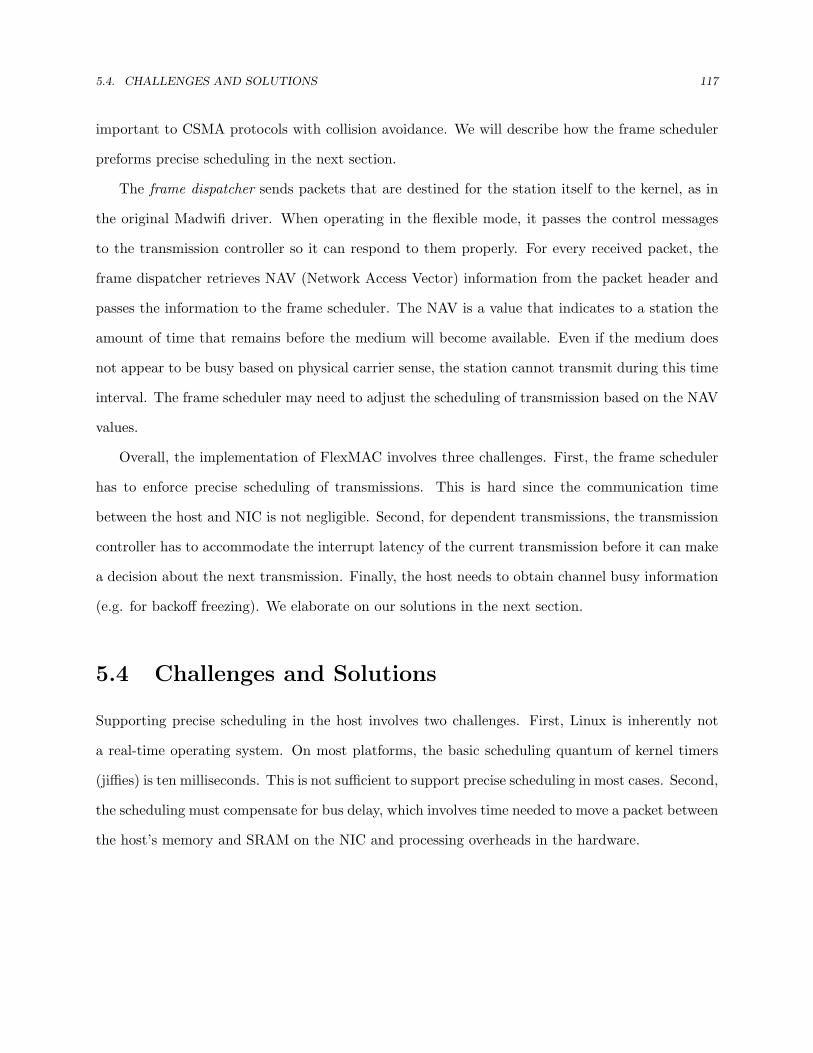
OPTIMIZING TRANSMISSION FOR WIRELESS VIDEO STREAMING

Mei-Hsuan Lu

A DISSERTATION

Submitted to the Department of Electrical and Computer Engineeringof Carnegie Mellon University

in partial fulfillment ofthe requirements for the degree of

DOCTOR OF PHILOSOPHY

July 2009

Committee:Prof. Tsuhan Chen, AdvisorProf. Peter Steenkiste, AdvisorProf. Ragunathan RajkumarDr. M. Reha Civanlar (Ozyegin University)

Copyright c©July 2009

Mei-Hsuan Lu

All rights reserved

ii

ABSTRACT

With advances in wireless networking technologies, wireless multimedia transmission has

grown dramatically in recent years. The simplicity, flexibility, and low up-front costs of such

systems have not only enabled mobility support for existing multimedia applications but

also stimulated the development of new wireless multimedia services. Despite having many

advantages, wireless multimedia services, particularly video services, also pose a number of

challenges that have prevented them from reaching their full potential. In this thesis, we

propose a novel framework that (1) efficiently uses available wireless resources by means of

cross-layer design in intermediate nodes, wireless relays, and end systems and (2) opportunis-

tically optimizes wireless resource use by leveraging path diversity with agile path selection

to support wireless video transmission.

The proposed solution consists of two building blocks: PRO and TAR. PRO (Protocol

for Retransmitting Opportunistically) is an efficient opportunistic retransmission protocol

residing in the MAC layer. Opportunistic retransmission employs overhearing nodes, if

any, distributed in physical space to function as relays that opportunistically retransmit

failed packets on behalf of the source. Relays with better connectivity to the destination

have a higher chance of delivering packets successfully than the source does, thereby result-

ing in a more efficient use of the channel. TAR (Time-based Adaptive Retransmission) is

a MAC-centric cross-layer strategy that leverages application-level information to improve

MAC (re)transmission. As the name suggests, TAR dynamically determines whether to

(re)transmit or discard a packet based on the retransmission deadline of the packet assigned

by the video server regardless of how many trials have been issued for the packet. TAR

significantly reduces the number of late packets and avoids using scarce wireless bandwidth

to retransmit useless packets. The ultimate solution, PROTAR is a seamless combination of

PRO and TAR that further pushes the performance envelope.

To illustrate the efficacy of the proposed solutions, analytical results, testbed experimen-

iii

tal results, real-world experimental results, and user studies of subjective video quality for

a wide range of wireless scenarios are conducted. The evaluation results consistently show

that PRO and TAR can contribute individually. Moreover, PROTAR provides further per-

formance gain in network throughput and visual quality, especially in contended channels,

under fading, or with user mobility.

iv

ACKNOWLEDGMENTS

I always feel I am so lucky to have two advisors who guide me in my Ph.D studies.

They are like two parents in a child’s growth, both of whom are unreplaceable. Professor

Tsuhan Chen as my advisor was a source of inspiration and ideas. His extremely successful

professional life has been a strong motivating factor in pursuit of my Ph.D. From him, I’ve

learned that good research is not about intricate equations that only few can digest but simple

yet effective solutions that everyone can appreciate. Tsuhan is not only a great advisor but

also a caring mentor during my Ph.D. His strong dedication, amazing energy, warmth, and

generosity will continue to be the source of inspiration to me. I am also extremely grateful

to my co-advisor, Professor Peter Steenkiste, without whom this dissertation will not be

possible. Peter is knowledgeable, patient, kind, and responsible. I can discuss a broad range

of problems with him, ranging from big picture questions to possible causes of a bug. From

him, I learned not only research methodologies but also speaking and writing skills that I

will continue to benefit from in my future career. It is Peter’s kind encouragements and

insightful directions that helped me overcome various barriers during my thesis research.

I would also like to thank other members in my thesis committee – Professor Ragunathan

Rajkumar and Dr. M. Reha Civanlar, for their valuable feedback and suggestions that helped

me to improve the overall quality of this thesis. Special thanks to Professor Ozan Tonguz

who is always helpful. I also want to thank former AMP members Deepak Turaga, Trista

Chen, and Ta-Chien Lin for their assistance in my research and future career plan. It was a

great pleasure knowing you.

This thesis was supported in part by the Institute for Information Industry (III), HP

Labs, the International Collaboration for Advancing Security Technology (iCAST), and an

NSF grant. I am grateful to these sponsors for their support.

I would like to thank other members in Tsuhan’s group, David Liu, Kate Shim, Wende

Zhang, Qi Wu, Wei Yu, Kevin Chang, Andrew Gallagher, Devi Parikh, Congcong Li, Dhruv

v

Batra, and Yimeng Zhang, who provided feedback on my thesis and presentations. I would

also like to thank fellow students in Peter’s group, Glenn Judd, Xiaohui Wang, Fahad Dogar,

Xi Liu, Kaushik Lakshminarayanan, George Nychis, and Kevin Borris. In particular, I would

like to thank Xiaohui Wang, for her help on setting up emulation-based experiments during

the later stage of my thesis work. I would also like to thank all the good friends I made

in Pittsburgh, Yu-Hsiang Bosco Chiu, Juhua Liu, Hsin-Mu Tsai, Frank Wang, Ting-Fang

Yen, Chen-Ling Chou, Hung-Chih Lai, Yen-Tzu Lin, Mike Kuo, Lena Kim, and Cheng-Yuan

Wen for adding the element of fun in my Ph.D. life. Most of them also help me on tedious

user studies for video quality assessment. Many thanks to Hsin-Mu Tsai for his help on

OPNET-related problems. I want to thank my best friend, Anli Su, for her support and

accompany over these years.

Finally, I want to thank my family, my parents, my sister, and my brother. It is their

love, encouragements, and support that enable me to focus on my research and help tide me

through several rough patches. This thesis is dedicated to my parents.

vi

Contents

Chapter 1: Introduction 1

1.1 Challenges with Video Transmission . . . . . . . . . . . . . . . . . . . . . . . . . . . 2

1.1.1 Strict Timing Constraints . . . . . . . . . . . . . . . . . . . . . . . . . . . . . 2

1.1.2 High Bandwidth Demand . . . . . . . . . . . . . . . . . . . . . . . . . . . . . 2

1.1.3 Need for Unequal Error Protection . . . . . . . . . . . . . . . . . . . . . . . . 3

1.2 Challenges with Wireless Communication . . . . . . . . . . . . . . . . . . . . . . . . 3

1.2.1 Multi-path Fading and Shadowing . . . . . . . . . . . . . . . . . . . . . . . . 3

1.2.2 Limited Bandwidth . . . . . . . . . . . . . . . . . . . . . . . . . . . . . . . . 4

1.2.3 Interference . . . . . . . . . . . . . . . . . . . . . . . . . . . . . . . . . . . . . 4

1.2.4 User Mobility . . . . . . . . . . . . . . . . . . . . . . . . . . . . . . . . . . . . 4

1.3 Related Work . . . . . . . . . . . . . . . . . . . . . . . . . . . . . . . . . . . . . . . . 6

1.4 Scope of the Thesis . . . . . . . . . . . . . . . . . . . . . . . . . . . . . . . . . . . . . 14

1.4.1 Wireless Networking Environment . . . . . . . . . . . . . . . . . . . . . . . . 14

1.4.2 Video Streaming Applications . . . . . . . . . . . . . . . . . . . . . . . . . . . 14

1.5 Proposed Solutions . . . . . . . . . . . . . . . . . . . . . . . . . . . . . . . . . . . . . 15

1.5.1 Opportunistic Retransmission . . . . . . . . . . . . . . . . . . . . . . . . . . . 16

1.5.2 Time-based Adaptive Retransmission . . . . . . . . . . . . . . . . . . . . . . 17

1.5.3 Time-based Opportunistic Retransmission . . . . . . . . . . . . . . . . . . . . 17

1.6 Thesis Statement . . . . . . . . . . . . . . . . . . . . . . . . . . . . . . . . . . . . . . 18

1.7 Contributions . . . . . . . . . . . . . . . . . . . . . . . . . . . . . . . . . . . . . . . . 18

vii

1.8 Thesis Organization . . . . . . . . . . . . . . . . . . . . . . . . . . . . . . . . . . . . 19

Chapter 2: Opportunistic Retransmission 21

2.1 Basic Concept . . . . . . . . . . . . . . . . . . . . . . . . . . . . . . . . . . . . . . . . 21

2.2 Related Work . . . . . . . . . . . . . . . . . . . . . . . . . . . . . . . . . . . . . . . . 22

2.3 Analysis . . . . . . . . . . . . . . . . . . . . . . . . . . . . . . . . . . . . . . . . . . . 24

2.4 Protocol Design . . . . . . . . . . . . . . . . . . . . . . . . . . . . . . . . . . . . . . . 29

2.4.1 Link Quality Estimation . . . . . . . . . . . . . . . . . . . . . . . . . . . . . . 31

2.4.2 Relay Qualification . . . . . . . . . . . . . . . . . . . . . . . . . . . . . . . . . 33

2.4.3 Relay Selection . . . . . . . . . . . . . . . . . . . . . . . . . . . . . . . . . . . 35

2.4.4 Relay Prioritization . . . . . . . . . . . . . . . . . . . . . . . . . . . . . . . . 38

2.4.5 Retransmission . . . . . . . . . . . . . . . . . . . . . . . . . . . . . . . . . . . 38

2.4.6 Dynamic Switching between PRO and Mesh Networking . . . . . . . . . . . . 40

2.5 Network-Specific Issues . . . . . . . . . . . . . . . . . . . . . . . . . . . . . . . . . . . 40

2.5.1 Collision Avoidance . . . . . . . . . . . . . . . . . . . . . . . . . . . . . . . . 40

2.5.2 Fairness . . . . . . . . . . . . . . . . . . . . . . . . . . . . . . . . . . . . . . . 45

2.5.3 Incentive to Relay . . . . . . . . . . . . . . . . . . . . . . . . . . . . . . . . . 49

2.5.4 Hidden Terminal Effect . . . . . . . . . . . . . . . . . . . . . . . . . . . . . . 50

2.5.5 Multi-rate PRO . . . . . . . . . . . . . . . . . . . . . . . . . . . . . . . . . . . 51

2.6 Performance Evaluation . . . . . . . . . . . . . . . . . . . . . . . . . . . . . . . . . . 53

2.6.1 Testbed Experimental Results . . . . . . . . . . . . . . . . . . . . . . . . . . . 54

2.6.2 Real-world Experiment Results . . . . . . . . . . . . . . . . . . . . . . . . . . 64

2.7 Summary . . . . . . . . . . . . . . . . . . . . . . . . . . . . . . . . . . . . . . . . . . 72

Chapter 3: Time-based Adaptive Retransmission 73

3.1 Basic Concept . . . . . . . . . . . . . . . . . . . . . . . . . . . . . . . . . . . . . . . . 73

3.2 Related Work . . . . . . . . . . . . . . . . . . . . . . . . . . . . . . . . . . . . . . . . 75

3.3 Analysis . . . . . . . . . . . . . . . . . . . . . . . . . . . . . . . . . . . . . . . . . . . 76

3.4 Protocol Design . . . . . . . . . . . . . . . . . . . . . . . . . . . . . . . . . . . . . . . 81

viii

3.4.1 Assuring Standard Channel Access Behavior . . . . . . . . . . . . . . . . . . 82

3.4.2 Retrieving Retransmission Deadlines . . . . . . . . . . . . . . . . . . . . . . . 84

3.5 Assigning Retransmission Deadlines . . . . . . . . . . . . . . . . . . . . . . . . . . . 85


3.6.1 Testbed Experimental Results . . . . . . . . . . . . . . . . . . . . . . . . . . . 87

3.6.2 Real-world Experiment Results . . . . . . . . . . . . . . . . . . . . . . . . . . 94

3.7 Summary . . . . . . . . . . . . . . . . . . . . . . . . . . . . . . . . . . . . . . . . . . 95

Chapter 4: Time-based Opportunistic Retransmission 99

4.1 Basic Concept . . . . . . . . . . . . . . . . . . . . . . . . . . . . . . . . . . . . . . . . 99

4.2 Analysis . . . . . . . . . . . . . . . . . . . . . . . . . . . . . . . . . . . . . . . . . . . 100

4.3 Protocol Design . . . . . . . . . . . . . . . . . . . . . . . . . . . . . . . . . . . . . . . 100

4.3.1 Retransmission from Relays . . . . . . . . . . . . . . . . . . . . . . . . . . . . 101

4.3.2 Retrieving Retransmission Deadlines . . . . . . . . . . . . . . . . . . . . . . . 102


4.4.1 Testbed PSNR Results . . . . . . . . . . . . . . . . . . . . . . . . . . . . . . . 104

4.4.2 Real-World PSNR Results . . . . . . . . . . . . . . . . . . . . . . . . . . . . . 105

4.4.3 User Studies . . . . . . . . . . . . . . . . . . . . . . . . . . . . . . . . . . . . 106

4.5 Summary . . . . . . . . . . . . . . . . . . . . . . . . . . . . . . . . . . . . . . . . . . 111

Chapter 5: Implementation 112

5.1 Background . . . . . . . . . . . . . . . . . . . . . . . . . . . . . . . . . . . . . . . . . 112

5.2 Related Work . . . . . . . . . . . . . . . . . . . . . . . . . . . . . . . . . . . . . . . . 114

5.3 Design . . . . . . . . . . . . . . . . . . . . . . . . . . . . . . . . . . . . . . . . . . . . 114

5.4 Challenges and Solutions . . . . . . . . . . . . . . . . . . . . . . . . . . . . . . . . . . 117

5.4.1 Supporting Precise Scheduling . . . . . . . . . . . . . . . . . . . . . . . . . . 118

5.4.2 Handling Dependent Transmissions . . . . . . . . . . . . . . . . . . . . . . . . 119

5.4.3 Determining the State of Use of the Channel . . . . . . . . . . . . . . . . . . 121

5.5 Precision of FlexMAC . . . . . . . . . . . . . . . . . . . . . . . . . . . . . . . . . . . 122

ix

5.5.1 Timing Precision . . . . . . . . . . . . . . . . . . . . . . . . . . . . . . . . . . 123

5.5.2 Throughput . . . . . . . . . . . . . . . . . . . . . . . . . . . . . . . . . . . . . 125

5.5.3 Coexistence with Hardware MAC and Software MAC . . . . . . . . . . . . . 126

5.5.4 Hidden Terminal Effect . . . . . . . . . . . . . . . . . . . . . . . . . . . . . . 126

5.6 Protocol Implementation Details . . . . . . . . . . . . . . . . . . . . . . . . . . . . . 128

5.6.1 Protocol for Retransmitting Opportunistically (PRO) . . . . . . . . . . . . . 129

5.6.2 Time-based Adaptive Retransmission (TAR) . . . . . . . . . . . . . . . . . . 129

5.6.3 Time-based Opportunistic Retransmission (PROTAR) . . . . . . . . . . . . . 130

5.7 Summary . . . . . . . . . . . . . . . . . . . . . . . . . . . . . . . . . . . . . . . . . . 130

Chapter 6: Conclusions and Future Work 131

6.1 Contribution . . . . . . . . . . . . . . . . . . . . . . . . . . . . . . . . . . . . . . . . 131

6.2 Future Work . . . . . . . . . . . . . . . . . . . . . . . . . . . . . . . . . . . . . . . . 134

6.2.1 Sophisticated Multi-rate Opportunistic Retransmission . . . . . . . . . . . . . 134

6.2.2 Opportunistic Retransmission with Networking Coding . . . . . . . . . . . . 134

6.2.3 Cooperative Application-Layer Relaying . . . . . . . . . . . . . . . . . . . . . 135

Chapter A: Review of the IEEE 802.11 Standard 149

A.1 Basic Channel Access . . . . . . . . . . . . . . . . . . . . . . . . . . . . . . . . . . . 149

A.2 Error Recovery and Retry Limit . . . . . . . . . . . . . . . . . . . . . . . . . . . . . 151

A.3 Rate Adaptation . . . . . . . . . . . . . . . . . . . . . . . . . . . . . . . . . . . . . . 152

x

List of Figures

1.1 Related work categories: overview . . . . . . . . . . . . . . . . . . . . . . . . . . . . 5

2.1 A four-node network with link error rates shown along the edges of the graph . . . . 22

2.2 State transition diagram of a four-node network . . . . . . . . . . . . . . . . . . . . . 26

2.3 Network with an 8× 8 square grid topology . . . . . . . . . . . . . . . . . . . . . . . 28

2.4 Comparison of packet loss rates of an 8× 8 square grid topology . . . . . . . . . . . 28

2.5 Protocol flowchart of PRO . . . . . . . . . . . . . . . . . . . . . . . . . . . . . . . . . 29

2.6 Measurement results of packet delivery ratio and RSSI . . . . . . . . . . . . . . . . . 32

2.7 Periodic Broadcast Message Format . . . . . . . . . . . . . . . . . . . . . . . . . . . 36

2.8 Relay collision probability . . . . . . . . . . . . . . . . . . . . . . . . . . . . . . . . . 43

2.9 Successful retransmission probability . . . . . . . . . . . . . . . . . . . . . . . . . . . 44

2.10 Backoff intervals distribution from multiple relays . . . . . . . . . . . . . . . . . . . . 47

2.11 Non-uniform backoff intervals distribution of individual relays . . . . . . . . . . . . . 47

2.12 Impact on fairness . . . . . . . . . . . . . . . . . . . . . . . . . . . . . . . . . . . . . 48

2.13 Number of eligible relays and expected number of active eligible relay . . . . . . . . 49

2.14 Illustration of table lookup in multi-rate PRO . . . . . . . . . . . . . . . . . . . . . . 52

2.15 Static scenario topology . . . . . . . . . . . . . . . . . . . . . . . . . . . . . . . . . . 54

2.16 UDP throughput over different source-destination distances . . . . . . . . . . . . . . 55

2.17 UDP throughput . . . . . . . . . . . . . . . . . . . . . . . . . . . . . . . . . . . . . . 57

2.18 Successful retransmission ratio . . . . . . . . . . . . . . . . . . . . . . . . . . . . . . 57

2.19 Per-relay retransmission rates . . . . . . . . . . . . . . . . . . . . . . . . . . . . . . . 59

xi

2.20 Percentage of opportunistic retransmissions . . . . . . . . . . . . . . . . . . . . . . . 59

2.21 Mobile scenario test topology . . . . . . . . . . . . . . . . . . . . . . . . . . . . . . . 60

2.22 Throughput result of the mobile scenario . . . . . . . . . . . . . . . . . . . . . . . . 60

2.23 Fairness comparison . . . . . . . . . . . . . . . . . . . . . . . . . . . . . . . . . . . . 62

2.24 Experimental floor plan of the office building scenario . . . . . . . . . . . . . . . . . 64

2.25 Snapshot of the office building experiment setup . . . . . . . . . . . . . . . . . . . . 65

2.26 Throughput CDF results of single source/destination pair in an office building . . . 66

2.27 Throughput CDF results of concurrent source/destination pairs in an office building 66

2.28 Experimental floor plan of the student lounge . . . . . . . . . . . . . . . . . . . . . . 67

2.29 Snapshot of the student lounge experiment setup . . . . . . . . . . . . . . . . . . . . 68

2.30 Throughput CDF results of single source/destination pair in a student lounge . . . . 69

2.31 Throughput CDF of single session scenario in an office building (802.11g) . . . . . . 71

2.32 Throughput CDF of concurrent session scenario in an office building (802.11g) . . . 71

2.33 Throughput CDF of single session scenario in a student lounge (802.11g) . . . . . . . 71

3.1 Example of packet transmission outcomes . . . . . . . . . . . . . . . . . . . . . . . . 77

3.2 802.11 optimal retry limit as a function of µ/λ with variable packet error rates . . . 80

3.3 Loss rate comparison of TAR and 802.11 . . . . . . . . . . . . . . . . . . . . . . . . . 81

3.4 Protocol operation of TAR . . . . . . . . . . . . . . . . . . . . . . . . . . . . . . . . 81

3.5 TAR preserves equal channel access behavior as the 802.11 . . . . . . . . . . . . . . 83

3.6 Overview of the 802.11 protocol . . . . . . . . . . . . . . . . . . . . . . . . . . . . . . 85

3.7 Testbed topology used for studying the 802.11 retransmission issues . . . . . . . . . 87

3.8 Statistics of packets generated from emu-5 in the general scenario . . . . . . . . . . . 88

3.9 Topology of a simple scenario . . . . . . . . . . . . . . . . . . . . . . . . . . . . . . . 90

3.10 Topology of a mobile user scenario scneario . . . . . . . . . . . . . . . . . . . . . . . 90

3.11 Topology of a congested scenario . . . . . . . . . . . . . . . . . . . . . . . . . . . . . 90

3.12 Single session dynamic environment result . . . . . . . . . . . . . . . . . . . . . . . . 93

3.13 Real-world test topology . . . . . . . . . . . . . . . . . . . . . . . . . . . . . . . . . . 93

3.14 Distribution of valid, late and lost packets . . . . . . . . . . . . . . . . . . . . . . . . 96

xii

3.15 Real-world results for unequal error protection . . . . . . . . . . . . . . . . . . . . . 97

3.16 Real-world result of PSNR values . . . . . . . . . . . . . . . . . . . . . . . . . . . . . 98

4.1 Loss rate comparison of an N ×N square grid topology . . . . . . . . . . . . . . . . 101

4.2 System diagram of PROTAR . . . . . . . . . . . . . . . . . . . . . . . . . . . . . . . 102

4.3 802.11 MAC frame with time to relay (TTR) field . . . . . . . . . . . . . . . . . . . 103

4.4 Single session result . . . . . . . . . . . . . . . . . . . . . . . . . . . . . . . . . . . . 107

4.5 Concurrent session result . . . . . . . . . . . . . . . . . . . . . . . . . . . . . . . . . 108

4.6 Single session mobile client result . . . . . . . . . . . . . . . . . . . . . . . . . . . . . 109

4.7 Single session dynamic environment result . . . . . . . . . . . . . . . . . . . . . . . . 110

5.1 System Diagram of FlexMAC . . . . . . . . . . . . . . . . . . . . . . . . . . . . . . . 115

5.2 Timing of a transmission (ignoring propagation delay) . . . . . . . . . . . . . . . . . 118

5.3 Histogram of bus delay . . . . . . . . . . . . . . . . . . . . . . . . . . . . . . . . . . . 120

5.4 Histogram of interrupt latency in transmitting packets . . . . . . . . . . . . . . . . . 120

5.5 Histogram of interrupt latency in receiving packets . . . . . . . . . . . . . . . . . . . 120

5.6 Inter-frame timing . . . . . . . . . . . . . . . . . . . . . . . . . . . . . . . . . . . . . 122

5.7 CDF of timing error . . . . . . . . . . . . . . . . . . . . . . . . . . . . . . . . . . . . 124

5.8 Collision Ratio . . . . . . . . . . . . . . . . . . . . . . . . . . . . . . . . . . . . . . . 127

5.9 Share of bandwidth in a mixed scenario . . . . . . . . . . . . . . . . . . . . . . . . . 127

5.10 Histogram of backoff interval . . . . . . . . . . . . . . . . . . . . . . . . . . . . . . . 127

6.1 Example of networking coding . . . . . . . . . . . . . . . . . . . . . . . . . . . . . . . 135

A.1 The 802.11 basic channel access . . . . . . . . . . . . . . . . . . . . . . . . . . . . . . 150

A.2 Exponential increase of contention window [1] . . . . . . . . . . . . . . . . . . . . . . 151

A.3 Overview of the 802.11 protocol . . . . . . . . . . . . . . . . . . . . . . . . . . . . . . 152

xiii

List of Tables

2.1 System states of the four-node network (N = 4) in Figure 2.1 . . . . . . . . . . . . . 25

2.2 Overall collision probabilities . . . . . . . . . . . . . . . . . . . . . . . . . . . . . . . 58

2.3 On-line calibration result (offset to the default threshold) . . . . . . . . . . . . . . . 58

3.1 Testbed results of packet ratios . . . . . . . . . . . . . . . . . . . . . . . . . . . . . . 91

3.2 Testbed results of PSNR values . . . . . . . . . . . . . . . . . . . . . . . . . . . . . . 92

4.1 Testbed objective visual quality results . . . . . . . . . . . . . . . . . . . . . . . . . . 105

4.2 Real-world objective visual quality results . . . . . . . . . . . . . . . . . . . . . . . . 105

4.3 Attributes of visual quality scale . . . . . . . . . . . . . . . . . . . . . . . . . . . . . 106

4.4 Summary of performance over different real-world scenarios . . . . . . . . . . . . . . 111

5.1 Throughput results . . . . . . . . . . . . . . . . . . . . . . . . . . . . . . . . . . . . . 125

5.2 Hidden terminal results . . . . . . . . . . . . . . . . . . . . . . . . . . . . . . . . . . 126

1

Chapter 1

Introduction

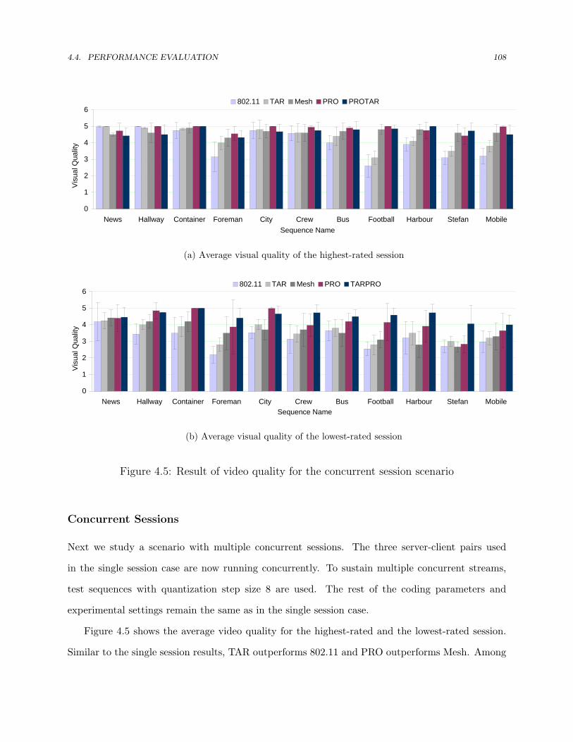
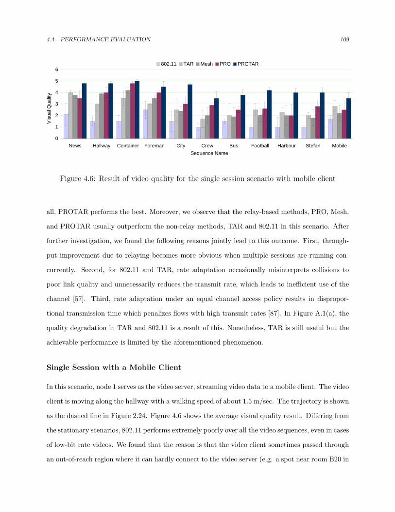
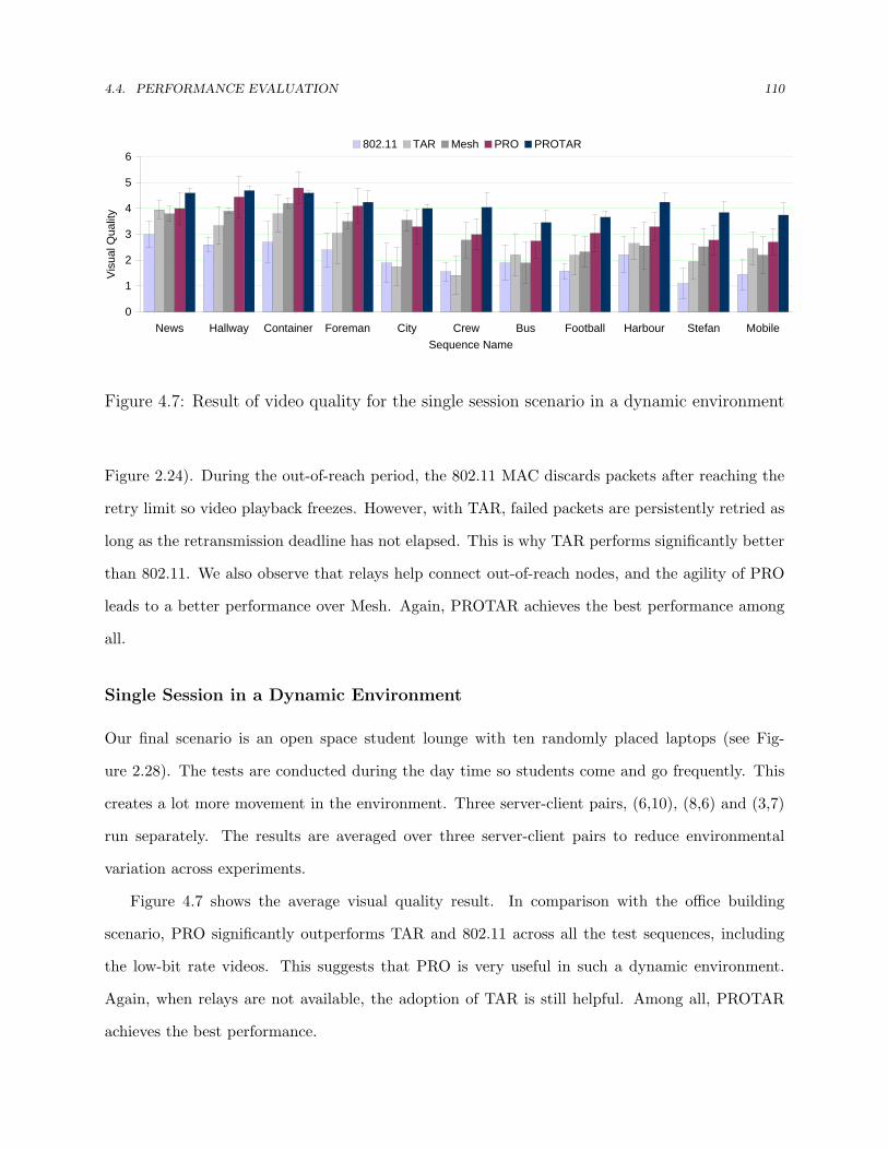
With advances in wireless networking technologies, wireless multimedia transmission has grown

dramatically in recent years. The simplicity, flexibility, and low up-front costs of such systems have

not only enabled mobility support for existing multimedia applications but also stimulated the

development of new wireless multimedia services. Some representative examples include: (1) Video

telephony using portable wireless devices has become an appealing type of telecommunication;

(2) Video streaming of news and movie clips to mobile phones is now widely available; (3) A

wireless local area network (WLAN) can connect various audiovisual entertainment devices in a

home; and (4) Real-time audiovisual communication over wireless ad-hoc networks can direct and

supervise paramedics in providing life-support services in search-and-rescue and other disaster-

recovery operations. There are also applications of enterprise multimedia, community healthcare,

interactive gaming, remote teaching and training, augmented reality and many more that seem to

be announced on an almost daily basis. There is no doubt that wireless multimedia services have

become an essential part of our daily lives and will continue to pervade.

Despite having unleashed a plethora of new multimedia applications, wireless multimedia ser-

vices, particularly video services, continue to pose a number of challenges that have prevented

them from reaching their full potential. These challenges involve two aspects. First, video data

have specific service requirements that need to be fulfilled by the network. Second, the wireless

medium is a challenging environment for providing quality of service. The unique characteristics

1.1. CHALLENGES WITH VIDEO TRANSMISSION 2

of video data and wireless channels make wireless video transmission a difficult problem. In the

following two sections, we elaborate on each challenge in detail.

1.1 Challenges with Video Transmission

The service requirements of video applications differ significantly from those of the elastic ap-

plications (e-mail, Web, remote login, file sharing, etc.). Video applications have several unique

properties that are key to good performance:

1.1.1 Strict Timing Constraints

Most video applications are delay sensitive. For video telephony, gaming, or interactive video

applications, packets that incur a sender-to-receiver delay of more than a few hundred milliseconds

are essentially useless. Transmitting late packets whose timing constraints are violated wastes

bandwidth because late arrivals carry useless information, or at best, they are useful for concealing

errors in subsequent frames. What is worse, in a bandwidth-limited environment, sending late

packets can delay the transmissions of subsequent valid packets and potentially create more late

arrivals. Meeting timing constraints of video data is especially challenging over best-effort networks

which exhibit unpredictable delay, available bandwidth, or loss rates.

1.1.2 High Bandwidth Demand

Many video applications are bandwidth hungry. This is particularly true with the exploding de-

mand for applications like IPTV, gaming and business multimedia which use high quality video

displays. For example, a standard definition (SD) video stream typically runs at 3.75 megabits

per second (Mbps), while a high definition (HD) stream runs at 15 Mbps or more under MPEG-

2 encoding [2]. The high bandwidth demand makes video streaming over networks with limited

bandwidth a challenging problem.

1.2. CHALLENGES WITH WIRELESS COMMUNICATION 3

1.1.3 Need for Unequal Error Protection

One of the most powerful techniques for compressing video is inter-frame coding. Inter-frame coding

uses one or more earlier or later frames (reference frames) in a sequence to compress the current

frame. When the current frame contains areas where nothing has moved in the reference frame,

the system simply issues a short command that copies that part of the reference frame, into the

current one. Inter-frame coding is very efficient because subsequent video frames typically exhibit

high correlations.

Despite high compression efficiency, inter-frame coding also makes video data vulnerable to

losses. For inter-frame coded video streams, packet losses can result in different levels of degradation

in video quality. Specifically, loss in a reference frame is critical because it causes error propagation

across a sequence of video frames that are inter-coded with respect to the reference frame. As such,

video applications typically require unequal error protection for different types of video frames,

which is not supported by most wireless networks.

1.2 Challenges with Wireless Communication

Wireless networks have several important advantages over wired counterparts including ease of

deployment and support for mobile users. However, wireless communication also involves a number

of challenges. These challenges, coupled with the unique characteristics of video data, amplify the

difficulty of video transmission. In the following, we highlight some of the main challenges in

wireless networking and discuss their impact on video communication.

1.2.1 Multi-path Fading and Shadowing

Multi-path fading and shadowing are common wireless effects. Multi-path fading is due to multi-

path propagation: signals from different paths add constructively or destructively. This occurs

when, e.g., people moving around between the transmitter and the receiver. Multi-path fading

results in rapid fluctuation of signal amplitude within the order of a wavelength. Shadowing, on

the other hand, occurs over a relatively large time scale. It is caused by obstacles between the


transmitter and the receiver that attenuate signal power through absorption, reflection, scattering,

and diffraction. The presence of multi-path fading and shadowing results in time-varying channel

conditions and location-dependent packet erasures. This presence complicates the provision of

delay and bandwidth requirements for video applications.

1.2.2 Limited Bandwidth

Today’s wired networks can easily support bandwidths of multi-Gbps. However, wireless networks

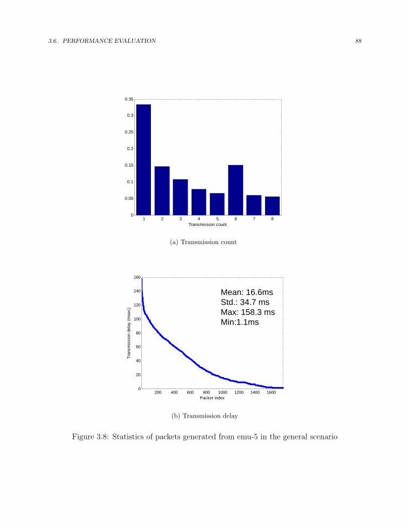
are more limited in capacity. The 802.11 products are advertised as having a data rate of 54

Mbps. However, “protection” mechanisms such as binary exponential backoff, rate adaptation, and

protocol overheads cut the throughput 50% or more. As indicated in [3], the actual throughput of

802.11a and 802.11g is up to 27 Mbps and 24 Mbps. In addition, owing to backward compatibility

with 802.11b, 802.11g is encumbered with legacy issues that reduce throughput by an additional

∼21%. Moreover, the actual bandwidth available to individual users can even be much lower due to

the shared nature of the wireless medium. This low bandwidth environment poses a great obstacle

for providing video services with high bandwidth requirements.

1.2.3 Interference

The wireless medium is essentially shared among multiple nodes, and hence, signals that arrive at

a receiver from other concurrent transmissions, albeit attenuated, constitute interference for the

receiver. Interference is a common effect in WLANs because they operate in the unlicensed 2.4/5

GHz ISM frequency band. WLAN devices share bandwidth with other devices, e.g. Bluetooth

peripheral devices, spread-spectrum cordless phones, or microwave ovens. Interference affects the

quality of a wireless link and, consequently, its error rate and achievable capacity.

1.2.4 User Mobility

User mobility is one of the obvious advantages of wireless networking. Wireless network users can

move around within a broad coverage area and still be connected to the network. In spite of its


End host End host

Application layer

tion

End host

Application layer

tion

End host

Transport layer

Network layer

ayer

inte

rac Transport layer

Network layer

ayer

inte

rac

MAC layerCro

ss la

MAC layerCro

ss la

(a) End-to-End view

End host End hostIntermediate node

Application layer

tion

End host

Application layer

tion

End hostIntermediate node

Application layer

Transport layer

Network layer

ayer

inte

rac Transport layer

Network layer

ayer

inte

rac

Network layer

Transport layer

erNetwork

MAC layerCro

ss la

MAC layerCro

ss la

MAC layer

Cro

ss la

yeLevel

Wired backhaul Wireless access network

(b) End-to-Intermediate-to-End view

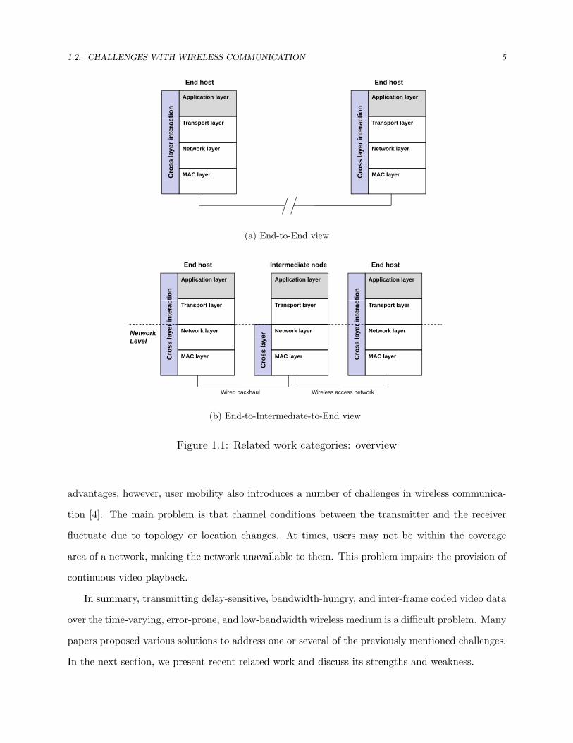
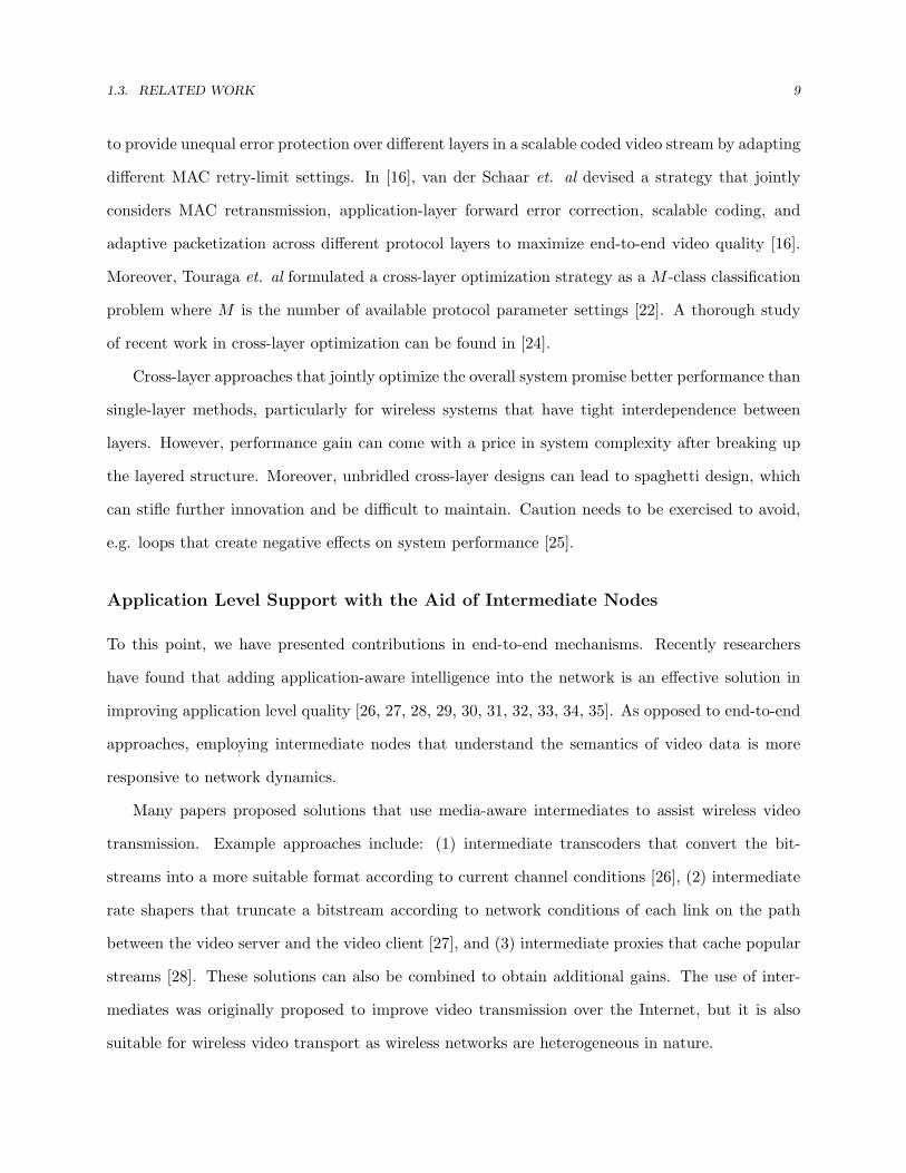
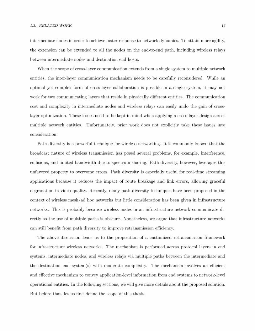
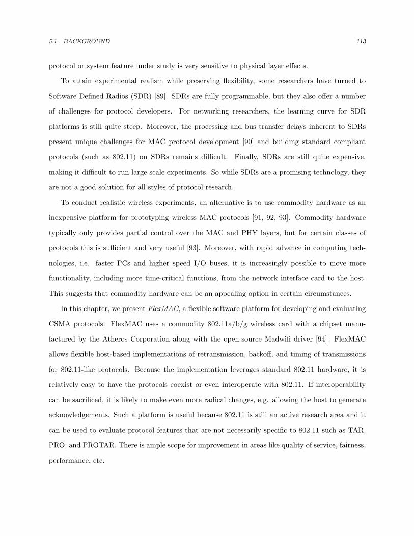
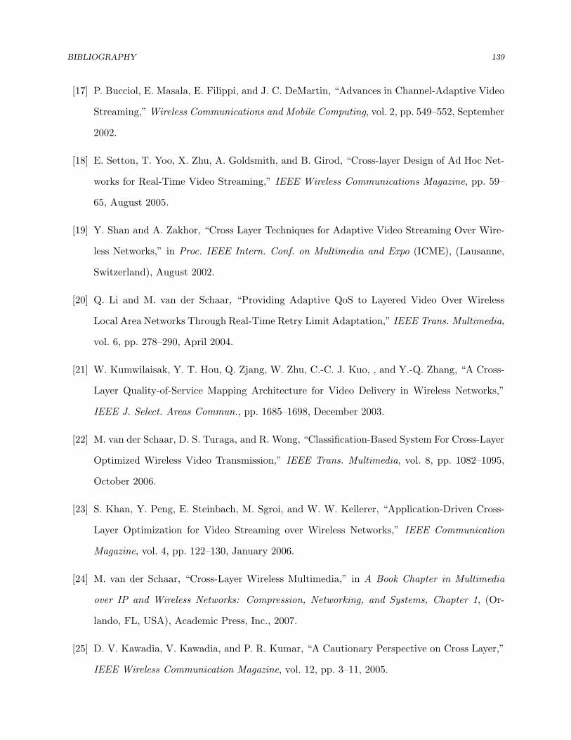
Figure 1.1: Related work categories: overview

advantages, however, user mobility also introduces a number of challenges in wireless communica-

tion [4]. The main problem is that channel conditions between the transmitter and the receiver

fluctuate due to topology or location changes. At times, users may not be within the coverage

area of a network, making the network unavailable to them. This problem impairs the provision of

continuous video playback.

In summary, transmitting delay-sensitive, bandwidth-hungry, and inter-frame coded video data

over the time-varying, error-prone, and low-bandwidth wireless medium is a difficult problem. Many

papers proposed various solutions to address one or several of the previously mentioned challenges.

In the next section, we present recent related work and discuss its strengths and weakness.

1.3. RELATED WORK 6

1.3 Related Work

There exists an extensive body of literature proposing different solutions addressing the challenges

of wireless video transmission. Generally, we can classify these research efforts in five categories: (1)

at the application level in end hosts, (2) across multiple layers in end hosts, (3) at the application

level with the aid of intermediate nodes, (4) across multiple layers in intermediate nodes, and (5) via

the exploitation of path diversity. Categories (1) and (2) are end-to-end solutions (Figure 1.1(a))

whereas (3), (4) and (5) involve the support from intermediate nodes (Figure 1.1(b)). In the

following, we elaborate on each of them.

Application Level in End Hosts

Solutions in this category work in the application layer in end hosts (video servers and video

clients) [5, 6, 7, 8, 9, 10, 11, 12, 13, 14, 15]. Some of these solutions assume knowledge of network

statistics to facilitate error control and bandwidth adaptation. These statistics can be measured

by the application or obtained from lower layers when available.

Error-resilience coding is one of the most representative application level solutions. In recent

video coding standards, error-resilient encoding and decoding strategies have been considered as an

important feature. For example, slice-structured coding, reference picture selection, data partition-

ing, and reversible variable-length coding are widely used error-resilience coding techniques [5, 6].

Coding with error-resilience capabilities yields a bitstream that is less vulnerable to channel er-

rors, but it comes at a price of transmitting more bits. It is therefore important to establish a

balance between error resilience and compression efficiency so as to maximize wireless transmission

performance.

For pre-coded videos without error-resilience capabilities embedded, error control for video data

may exploit error detection and retransmission (ARQ, Automatic Repeat reQuest) [7]1. The desti-

nation sends an acknowledgement (ACK) back to the source to indicate successful reception. If the

sender does not receive an ACK after a timeout, it retransmits the packet until it receives an ACK

1Most video applications use UDP because reliable data transfer is not absolutely critical for the ap-plication’s success and video transmission generally reacts very poorly to TCP’s congestion control. Thus,reliability is directly built in the application itself.

1.3. RELATED WORK 7

or exceeds a predefined number of retransmissions. If there is no feedback channel or the sender-to-

receiver delay is significant, forward error correction (FEC) coding is an alternative approach. In

systems that discard the whole MAC frame in error, video applications apply FEC encoding across

video packets using an interleaver. The resulting parity packets are then transmitted together with

the video packets to improve the error correction process at the receiver. To offer unequal error

protection, FEC codes with different error correction capabilities are applied to different layers of a

scalable-coded videos stream. In [15], Chen and Chen proposed a novel solution to allocate parity

bits more efficiently by taking the rate-distortion properties of video data into account. Contrary

to ARQ that trades delay for bandwidth efficiency, FEC trades bandwidth for latency to improve

the loss rate by alleviating late arrivals [8]. Hybrid ARQ (HARQ) is proposed as a scheme that

combines the reliability and fixed delay advantage of FEC with the conservative bandwidth use of

ARQ [9].

In addition to bit errors, wireless networks are hampered by bandwidth variation. Changes in

available bandwidth cause quality degradation, resulting in occasional to total service interruption.

Existing bandwidth adaptation techniques exploit video coding characteristics to achieve graceful

change in video quality. For instance, error-resilience transcoding converts a video bitstream into

a more resilient one that conforms to the available bandwidth by manipulating temporal, spatial,

and SNR trade-offs on-the-fly [10]. This technique can better utilize the available bit budget but

tends to be computationally expensive. A cheaper alternative for adapting transmit rates in re-

sponse to channel dynamics is selective dropping. This scheme drops bidirectional-predicted frames

(B-frames) first, predicted frames (P-frames) next, and intra-coded frames (I-frames) last [11]. For

pre-encoded videos, it is also possible to create multiple bitstreams with different bandwidth re-

quirements and select the most appropriate bitstream at run time based on channel quality [12].

Furthermore, when content-level information is available, video applications can apply region-of-

interest (ROI) scalable coding schemes and prioritize video contents of the most interest to end

users [13]. The basic concept behind these bandwidth adaptation methods is to give precedence to

important video data when bandwidth is insufficient to maximize received video quality.

Application-layer approaches are self-contained as they do not assume the support of lower

1.3. RELATED WORK 8

layers. Application-layer approaches are widely applicable over both wired or wireless network-

ing systems. However, performing optimization in the application level alone may only achieve

suboptimal performance. This is because:

• The resource management, adaptation, and protection strategies available in the lower layers

(physical (PHY) layer, media access control (MAC) layer, and network/transport layers) are

devised without explicitly considering the specific characteristics of video data [16].

• Video applications do not consider the mechanisms provided by the lower layers for error

protection, scheduling, resource management, and so on [17].

In the following subsection, we present recent research work along the line of cross-layer opti-

mization.

Multiple Layers in End Hosts

In recent years, researchers have proposed the idea of cross-layer design to combat the challenges

of wireless video transmission [18, 19, 20, 16, 21, 22, 23]. In this design, upper layers exchange in-

formation with lower layers such that operational modes and adaptation parameters is configured

to optimize system-wide performance. For example, routing protocols can avoid links experiencing

long latencies for transmitting delay-sensitive video data. While the conventional layered architec-

ture reduces network design complexity, multiple layers may replicate protection strategies, causing

unnecessary overheads. It is believed that a cross-layer design benefits video transmission over wire-

less networks with rapidly-varying channels and scarce resources.

Research on cross-layer optimization made significant progress since the year 2000. In [19], Shan

and Zakhor presented an adaptation mechanism in which an application layer packet is decomposed

exactly into an integer number of equal-sized radio link protocol (RLP) packets. FEC codes are

applied within an application packet at the RLP packet level rather than across different application

packets. This reduces delay at the receiver compared with application level FEC solutions. In [20],

Li and van der Schaar proposed a heuristic for determining the optimal MAC retry limit that

minimizes errors due to sending buffer overflow and link erasures. The proposed solution is extended

1.3. RELATED WORK 9

to provide unequal error protection over different layers in a scalable coded video stream by adapting

different MAC retry-limit settings. In [16], van der Schaar et. al devised a strategy that jointly

considers MAC retransmission, application-layer forward error correction, scalable coding, and

adaptive packetization across different protocol layers to maximize end-to-end video quality [16].

Moreover, Touraga et. al formulated a cross-layer optimization strategy as a M -class classification

problem where M is the number of available protocol parameter settings [22]. A thorough study

of recent work in cross-layer optimization can be found in [24].

Cross-layer approaches that jointly optimize the overall system promise better performance than

single-layer methods, particularly for wireless systems that have tight interdependence between

layers. However, performance gain can come with a price in system complexity after breaking up

the layered structure. Moreover, unbridled cross-layer designs can lead to spaghetti design, which

can stifle further innovation and be difficult to maintain. Caution needs to be exercised to avoid,

e.g. loops that create negative effects on system performance [25].

Application Level Support with the Aid of Intermediate Nodes

To this point, we have presented contributions in end-to-end mechanisms. Recently researchers

have found that adding application-aware intelligence into the network is an effective solution in

improving application level quality [26, 27, 28, 29, 30, 31, 32, 33, 34, 35]. As opposed to end-to-end

approaches, employing intermediate nodes that understand the semantics of video data is more

responsive to network dynamics.

Many papers proposed solutions that use media-aware intermediates to assist wireless video

transmission. Example approaches include: (1) intermediate transcoders that convert the bit-

streams into a more suitable format according to current channel conditions [26], (2) intermediate

rate shapers that truncate a bitstream according to network conditions of each link on the path

between the video server and the video client [27], and (3) intermediate proxies that cache popular

streams [28]. These solutions can also be combined to obtain additional gains. The use of inter-

mediates was originally proposed to improve video transmission over the Internet, but it is also

suitable for wireless video transport as wireless networks are heterogeneous in nature.

1.3. RELATED WORK 10

Similar to application-level solutions in end hosts, application-level support in intermediate

nodes does not assume any help from the network, so it is applicable in different types of networks.

Nevertheless, performance can be further improved by applying a cross-layer design in intermediate

nodes. In the following subsection, we present recent work on multiple layer support in intermediate

nodes.

Multiple Layer Support in Intermediate Nodes

Solutions in multi-layer support in intermediate nodes involve collaboration across protocol layers

in end systems and in intermediate nodes. The application layer in end hosts exchanges information

with lower layers in intermediate nodes such that operational modes and adaptation parameters are

configured to optimize end-to-end performance. This extension of cross-layer design in end systems

alone can provide significant improvements in decoded video quality.

Solutions in this category introduce media-aware intelligence in the base station of a cellular

network [30, 32, 36], in the access point of an infrastructure WLAN [37, 38], or in the wireless

routers in a mesh network [39]. Specifically, intermediate nodes allocate network-level transmission

and buffering resources to packets according to their importance to the decoded video quality. One

type of such technique applies prioritization over different types of video packets. High priority

packets are granted more transmission opportunists and are less likely to be dropped due to buffer

overflow. For example, in [30], Chakravorty et. al associated different retry limits and error

correction configurations with packets of different perceptual importance in the radio link layer

in cellular networks. This practice grants important frames that contribute more to receiving

quality better protection against errors. A similar technique is also used in [29]. In [40], Ou et. al

used a selective dropping strategy for wireless access in vehicle environments (WAVE) to prioritize

reference frames (I frames) when it is not possible to transmit all packets due to limited dwelling

time, heavy load, or difficult channel conditions.

Priority-based methods offer coarse-level service differentiation among packets. To achieve fine-

grained resource allocation, sophisticated scheduling methods at the packet level are employed.

Such methods assume that side information about video stream structures is available on interme-


diate nodes. This information is then used for scheduling and buffer management. For example,

in [36], Liebl et al. proposed a joint radio link buffer management and scheduling scheme for wireless

video streaming based on a rate-distortion model proposed in [41]. The scheduler searches for an

optimal combination of scheduling and dropping strategies for different end-to-end streaming op-

tions based on the importance of each packet. The computation of packet importance considers the

transmission history of dependent packets. This scheme is later enhanced with fairness provision-

ing among heterogenous sessions in [32]. In [42], Pahalawatta et. al formulated error concealment

strategies, channel quality estimation, and distortion information into a utility function which is

used by a gradient-based scheduler to make network-level transmission decisions in wireless base

stations.

In brief, multiple layer support in intermediate nodes can lead to further improvements in system

efficiency and individual quality. This type of technique is especially useful when an intermediate

node lies on the interface between two heterogenous networks, for example between wired backhaul

and wireless access networks. Similar to applying a cross-layer design in end systems, breaking up

the layered structure in intermediate nodes also increases system complexity, which may not always

be acceptable or feasible.

Through the Exploitation of Path Diversity

The contributions discussed so far focus on maximizing the efficient use of available resources along

a predetermined path. There is an alternative type of solution that uses additional or alternate

resources to improve wireless video transmission by means of path diversity. Specifically, path

diversity exploits multiple paths between end hosts such that the end-to-end application sees a

virtual average path, which exhibits a smaller variability in quality than any of the individual

paths. In wireless environments, errors and delays are mostly path dependent, so path diversity is

an effective technique for improving wireless communication.

For low-latency video communication, path diversity, coupled with careful co-design of video

coding and packetization, has been demonstrated to be very powerful in combating losses [39,

43, 44, 45, 46]. A path diversity system may use multiple paths at the same time [39, 44, 46] or


switch between them (site selection) [45, 47]. Path diversity allows traffic dispersion, improves fault

tolerance and enables link recovery for data delivery.

An important problem in path diversity is path selection. Most path diversity work assumes

the set of paths is given, which may not always be the case. In [48], Wei and Zakhor showed

that path selection is an NP hard problem, and to approximate the optimum, they presented a

heuristic multipath selection framework for streaming video over wireless ad-hoc networks. This

technique selects two node-disjoint paths with minimum concurrent packet losses by taking into

account their interference. Murthy et. al later improved the heuristics using different metrics for

multipath computation when different coding schemes are used [49].

Existing path diversity and path selection techniques have several shortcomings. First, they

overlook the potential impact on other legacy flows. For instance, when video quality is improved

by transmitting packets over two or more paths, the performance of other data flows is likely to

degrade due to increased interference. It is therefore important to understand how path diversity

techniques affect the rest of the network. Unfortunately, this issue is rarely considered in the

literature. Second, existing path selection algorithms only consider two paths. While this constraint

reduces the complexity of the problem, it also limits the potential gain from path diversity. Third,

paths are established in advance of packet transmission. Because path quality may change over

time, such proactive path selection is not agile enough to deal with channel dynamics.

Improving on Earlier Work

The above discussion suggests a cross-layer, multi-path design for wireless video transmission.

Moreover, the design should consist of agility, practicality, low overhead, and transparency to the

rest of the network.

Cross-layer design is a promising technique in optimizing resource efficiency. It is particularly

useful for wireless video communication where the application has unique service requirements

for networks that only have sparse resources. The efficacy of cross-layer design largely depends

on the knowledge of wireless network conditions. For wireless networks with dynamic channels,

cross-layer approaches have been extended from within end systems to across end systems and


intermediate nodes in order to achieve faster response to network dynamics. To attain more agility,

the extension can be extended to all the nodes on the end-to-end path, including wireless relays

between intermediate nodes and destination end hosts.

When the scope of cross-layer communication extends from a single system to multiple network

entities, the inter-layer communication mechanism needs to be carefully reconsidered. While an

optimal yet complex form of cross-layer collaboration is possible in a single system, it may not

work for two communicating layers that reside in physically different entities. The communication

cost and complexity in intermediate nodes and wireless relays can easily undo the gain of cross-

layer optimization. These issues need to be kept in mind when applying a cross-layer design across

multiple network entities. Unfortunately, prior work does not explicitly take these issues into

consideration.

Path diversity is a powerful technique for wireless networking. It is commonly known that the

broadcast nature of wireless transmission has posed several problems, for example, interference,

collisions, and limited bandwidth due to spectrum sharing. Path diversity, however, leverages this

unfavored property to overcome errors. Path diversity is especially useful for real-time streaming

applications because it reduces the impact of route breakage and link errors, allowing graceful

degradation in video quality. Recently, many path diversity techniques have been proposed in the

context of wireless mesh/ad hoc networks but little consideration has been given in infrastructure

networks. This is probably because wireless nodes in an infrastructure network communicate di-

rectly so the use of multiple paths is obscure. Nonetheless, we argue that infrastructure networks

can still benefit from path diversity to improve retransmission efficiency.

The above discussion leads us to the proposition of a customized retransmission framework

for infrastructure wireless networks. The mechanism is performed across protocol layers in end

systems, intermediate nodes, and wireless relays via multiple paths between the intermediate and

the destination end system(s) with moderate complexity. The mechanism involves an efficient

and effective mechanism to convey application-level information from end systems to network-level

operational entities. In the following sections, we will give more details about the proposed solution.

But before that, let us first define the scope of this thesis.

1.4. SCOPE OF THE THESIS 14

1.4 Scope of the Thesis

The topic of wireless video transmission is very broad. In the previous section, we have addressed

a number of issues in prior work and pointed out several directions for further improvement. Based

on that, this thesis proposes solutions that run across end hosts and network entities along the

end-to-end path(s). The proposed approaches can be applied in a range of wireless technologies.

In the following subsection, we describe the common features of these networks. The requirement

for video applications in support of the proposed solutions is presented afterward.

1.4.1 Wireless Networking Environment

This thesis considers wireless networks that have the following properties:

• Intermediate nodes and destinations are within one-hop transmission range of each other

although the link delivery probability may be low.

• Retransmission and feedback are used for error control.

These properties are very common in wireless networking technologies, for example, 802.11

wireless LANs [1], 802.11 wireless distribution systems (WDS) [1] and 802.11p wireless access

in vehicular environments (WAVE) [50]. For mesh networks such as ad hoc wireless networks

and 802.15.4 wireless PANs (Zigbee) [51], our solutions can be applied over each hop in a multi-

hop transmission. For illustration purposes, this thesis considers the IEEE 802.11 WLAN as the

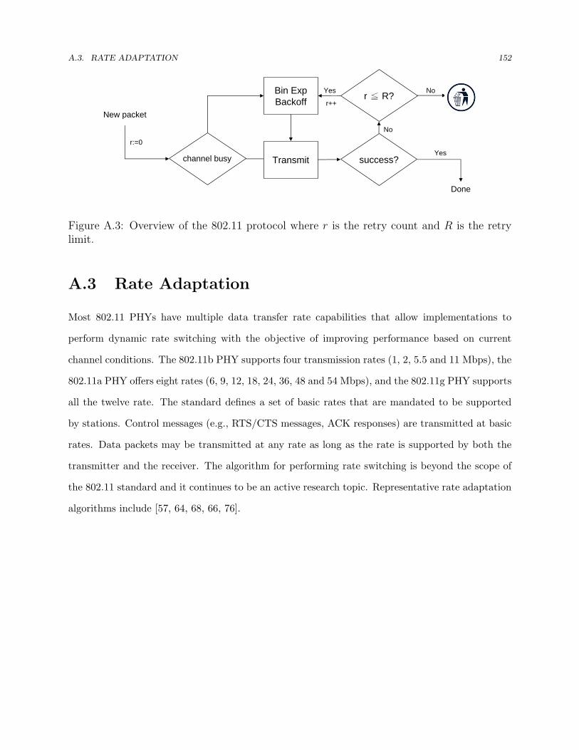
underlying wireless technology [1]. Appendix A will provide a brief review of the IEEE 802.11

protocol.

1.4.2 Video Streaming Applications

To support the proposed network-level solutions, we assume the video applications can communicate

with the MAC layer via information sharing. With application-level information, the MAC layer (in

the end system or in the intermediate nodes) operates in a way that maximizes user-perceived video

1.5. PROPOSED SOLUTIONS 15

quality. The video application may support error resilience coding or adaptive packet scheduling

to improve smooth playback on the video client side like most public streaming software [52, 53].

1.5 Proposed Solutions

We propose a novel network-level framework that (1) efficiently uses available wireless resources

by means of cross-layer design in intermediate nodes and in end systems and (2) opportunistically

optimizes wireless resource use by leveraging path diversity with agile path selection. We summarize

the main differences between our solution and prior work as follows:

• Practicability: We avoid complex cross-layer algorithms. Specifically, we combine temporal

and perceptual importance of video data into a single metric which is then used in the network

level for application-aware resource allocation. The use of a single metric allows cross-layer

optimization while preserving application abstraction in lower layers. This quality allows

immediate implementation in today’s commodity hardware.

• Agility: We adopt an agile path selection protocol for multipath transmission. Specifically,

paths are not predetermined but constructed opportunistically in the run time. Opportunistic

path selection has a number of advantages: First, it potentially allows the use of all possible

paths rather than limiting to several predetermined ones. Second, it rapidly adapts to the

best strategy when channel conditions change while proactive methods follow a strategy

based on average performance [16, 44]. This advantage is especially useful in time-varying,

rapidly-changing wireless environments.

• Transparency: Our solutions offer transparency to legacy nodes in the network. That is,

the adoption of our solutions do not affect short-term or long-term performance of legacy

traffic in the network. Prior work focuses on performance improvement for a single video

session (or a set of sessions) but overlooks the potential impact on the rest of the network.

For example, transmitting packets over multiple paths may lead to a different bandwidth

distribution over other single-path flows, leading to unfairness across flows [43, 44]. Our


solutions consider transparency in the protocol design.

In the following sections, we discuss the basic idea and design challenges of the proposed so-

lutions. We first describe an agile path diversity technique. We then describe a light-weight

cross-layer design. Finally, we present the ultimate solution that seamlessly combines the two.

Detailed descriptions of protocol operations will be presented in later chapters.

1.5.1 Opportunistic Retransmission

Opportunistic retransmission increases individual wireless transmission efficiency by exploiting path

diversity with agile path selection [54, 55]. The scheme employs overhearing nodes, if any, dis-

tributed in physical space to function as relays that retransmit packets in error on behalf of the

source [54]. Relays with better connectivity to the destination have a higher chance of delivering

packets successfully than the source does, thereby resulting in a more efficient use of the channel.

The rationale is the fact that in wireless networks, errors are often path or location dependent, so

transmissions that fail over one path may succeed over another path. Opportunistic retransmis-

sion exploits the benefit of multi-hop transmission but in contrast to traditional mesh networking

solutions, no routing overhead is involved.

We have designed an efficient opportunistic retransmission protocol (PRO, Protocol for Re-

transmitting Opportunistically) for 802.11-like networks. The protocol design involves two main

challenges. First, it requires an effective measure of link quality to decide whether a node is suitable

to serve as a relay. This metric must accurately reflect channel conditions in fast changing wireless

environments. Second, it requires efficient coordination of the retransmission process given that

there may be many candidate relays. The protocol needs to ensure the best relay that overheard

the transmission forwards the packet while avoiding simultaneous retransmission attempts that can

lead to duplicates or collisions.

PRO can be applied to any type of wireless network with retransmission. For illustration

purposes, this thesis considers an 802.11 WLAN environment. PRO includes several advantages.

First, the protocol increases individual throughput as well as network capacity in 802.11 WLANs,

which benefits video applications with high bandwidth demands. Second, the protocol leverages the


standard 802.11 operations to achieve various protocol functions so it involves low overhead. Third,

the protocol behaves reactively so it allows the use of the most suitable relay at any given time.

Last, the protocol makes least impact on legacy 802.11 flows by enforcing the protocol operations

transparent to the rest of the network. These properties make PRO an attractive solution over

existing approaches. A detailed description of PRO is provided in Chapter 2.

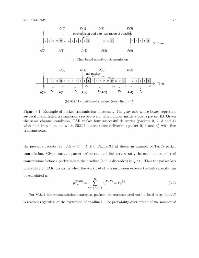
1.5.2 Time-based Adaptive Retransmission

Time-based Adaptive Retransmission (TAR) is a MAC-centric cross-layer mechanism that leverages

application-level information to improve MAC (re)transmission [24]. As the name suggests, TAR

dynamically determines whether to (re)transmit or discard a packet based on the retransmission

deadline of the packet assigned by the video server regardless of how many trials have been issued

for the packet [38, 37]. Unlike existing count-based retransmission strategies that adopt a fixed

retry limit, TAR dynamically adapts the maximum number of transmissions of a packet based on

current channel conditions and video characteristics. This significantly reduces the number of late

packets [29].

For illustration purposes, this thesis considers a TAR-enabled 802.11 MAC protocol. Our design

includes the following advantages. First, the protocol assigns transmission resources in terms

of application-specific requirements. Second, the protocol is easy to implement in commodity

hardware because it preserves the FIFO queueing discipline in the link layer, while other time-

based approaches tend to adopt a complicated scheduling algorithm [20, 32]. Third, the protocol

ensures that the time-based operation does not change the standard channel access behavior, so

it preserves long-term fairness as well as short-term collision avoidance. These properties make

TAR an attractive solution over existing approaches. A detailed description of TAR is provided in

Chapter 3.

1.5.3 Time-based Opportunistic Retransmission

TAR and PRO can individually improve the performance of wireless video applications. The

combined solution, time-based opportunistic retransmission (PROTAR) that jointly draws on the

1.6. THESIS STATEMENT 18

strength of TAR and PRO can further push the performance envelop [56]. PROTAR enables cross-

layer optimization in multi-path transmission through time-based relaying. The main challenge in

combining TAR and PRO is to guarantee consistent use of retransmission deadlines across multiple

relays given that the clock of individual relays may not be synchronized. This operation must have

low overhead so the gain of time-based retransmission is not compromised. We will show that

PROTAR provides significant performance improvement in both objective and perceptive quality

via extensive testbed and real-world experiments. A detailed description of PROTAR is given

in Chapter 4. Implementation details of PRO, TAR, and PROTAR on commodity hardware are

presented in Chapter 5.

1.6 Thesis Statement

Time-based opportunistic retransmission is an efficient protocol for improving performance of wire-

less video streaming. The protocol offers application awareness to collaborative relays that re-

transmit on behalf of the source to increase wireless transmission efficiency. The two building

blocks, a time-based transmission strategy and an opportunistic retransmission protocol, are self-

contained and they can work and contribute individually. Time-based opportunistic retransmission

can be easily implemented using commodity hardware. This solution significantly improves video

streaming quality over a wide range of wireless networks.

1.7 Contributions

This thesis makes the following technical contributions:

Design, Development and Evaluation of Time-based Adaptive Retransmission: We

present a time-based adaptive retransmission strategy for sending delay-sensitive data over wireless

networks, as well as an implementation of the protocol. We conduct extensive testbed and real-

world experiments to evaluate protocol performance.

Design, Development and Evaluation of Opportunistic Retransmission: We present

an opportunistic retransmission protocol for increasing individual throughput and overall network

1.8. THESIS ORGANIZATION 19

capacity, as well as an implementation of the protocol. We conduct extensive testbed and real-

world experiments to demonstrate the efficacy of the protocol. The protocol is shown to offer

significant gains in heavily loaded, fading channels or with user mobility. A preliminary multi-

rate opportunistic retransmission protocol that integrates rate adaptation [57] into opportunistic

retransmission is also presented.

Design, Development and Evaluation of Time-based Opportunistic Retransmission:

We present a powerful solution that seamlessly combines time-based adaptive retransmission and

opportunistic retransmission to further push the performance envelope, as well as an implementa-

tion of the protocol.

Probabilistic Analysis of the Proposed Protocols: In addition to protocol design and de-

velopment, we present a probabilistic analysis for time-based adaptive retransmission, opportunistic

retransmission, as well as time-based opportunistic retransmission.

Extensive User Studies of Subjective Video Quality: We present extensive user studies

of subjective video quality in addition to objective performance evaluation. The user studies are

performed for diverse wireless environments in order to understand the effectiveness of the proposed

solutions in different deployment scenarios.

Host-based Software Development Platform for 802.11-like Protocols: Finally, we

develop a flexible development and evaluation platform (called FlexMAC) for 802.11-like protocols

using commodity hardware. FlexMAC allows customization of functions such as backoff, retrans-

mission, and packet timing on a commodity platform. These functions are typically not accessible

to the public research community. FlexMAC is a useful tool for researchers who study protocol

features embedded in 802.11-like protocols.

1.8 Thesis Organization

This thesis proceeds as follows. In Chapter 2, we present opportunistic retransmission, including

the basic concept, analysis, protocol design, and evaluation results both on a testbed and in the

real world. In Chapter 3, we present time-based adaptive retransmission. In Chapter 4, we present

1.8. THESIS ORGANIZATION 20

time-based opportunistic retransmission that combines opportunistic retransmission and time-based

adaptive retransmission. In Chapter 5, we present the protocol development platform, FlexMAC,

a software MAC framework that enables implementation of the proposed protocols in the host.

Finally, we present conclusion remarks and discuss future work in Chapter 6.

21

Chapter 2

Opportunistic Retransmission

Video applications have high throughput requirements, even in compressed form. Many consumer

applications, for example, High-Definition TV (HDTV), require transmission bit rates of several

Mbps. In this chapter, we take a closer look at opportunistic retransmission, a novel link-layer

multi-path transmission protocol that increases individual throughput as well as overall capacity

of wireless networks. We begin by describing the basic concept of opportunistic retransmission

and compare it with related work that falls in the context of opportunistic communication. We

then present an analysis to quantify the potential gain of opportunistic retransmission. We present

an efficient opportunistic retransmission protocol, followed by a discussion of several issues ad-

dressed in the protocol design. We present experimental results for PRO-enabled 802.11 WLANs

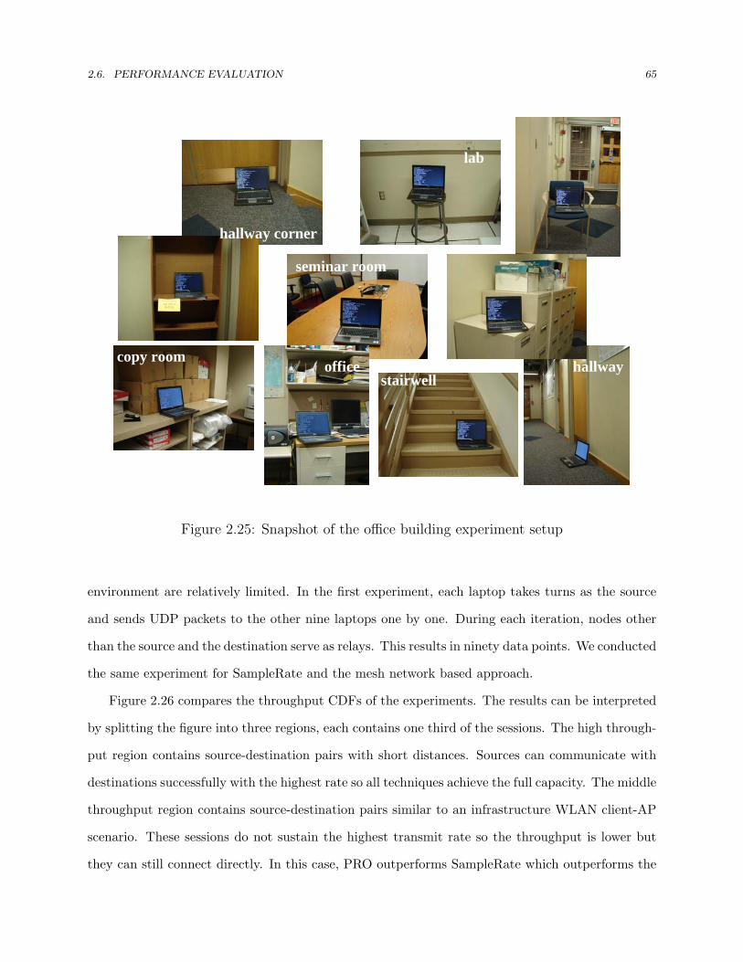
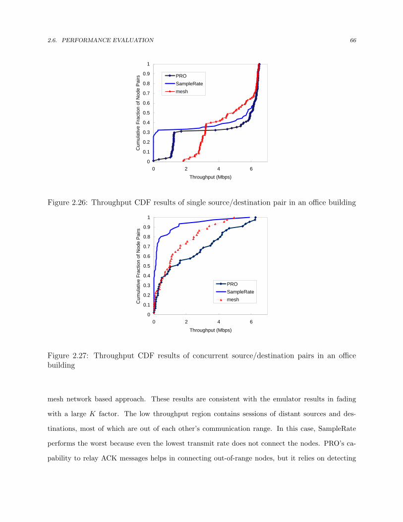
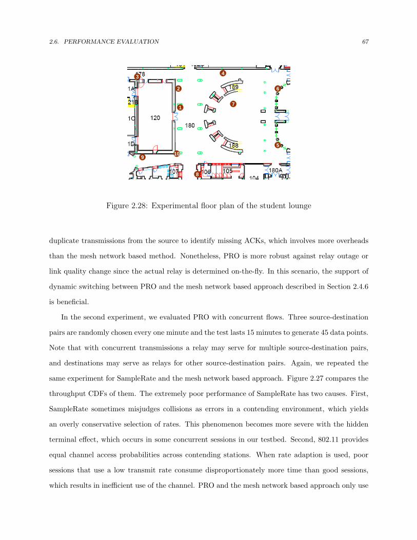
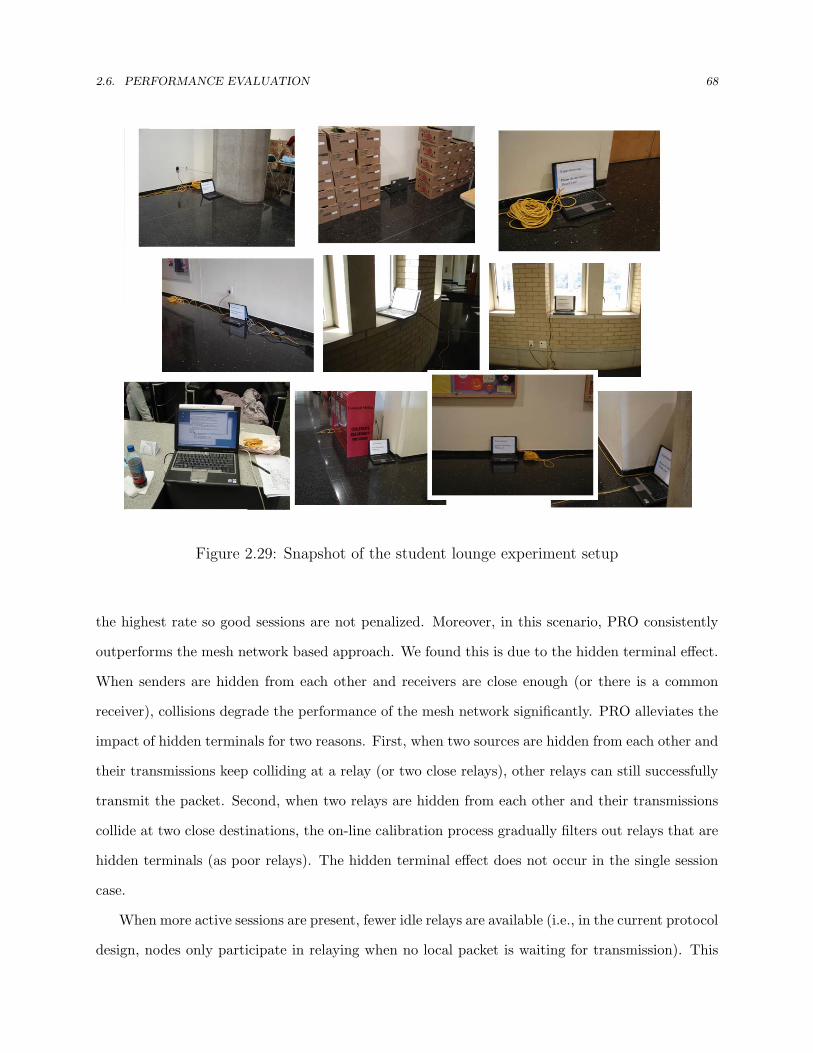
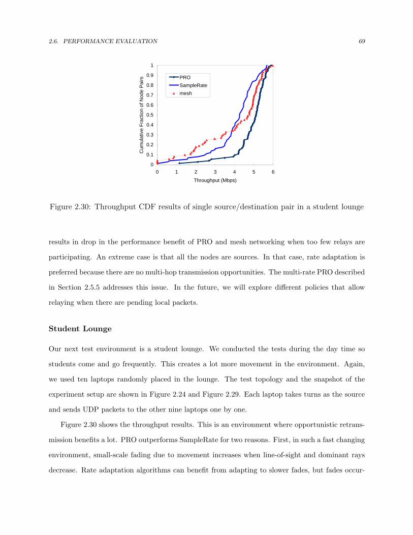
to demonstrate the effectiveness of the proposed schemes. Finally, we summarize this chapter.

2.1 Basic Concept

Opportunistic retransmission leverages the fact that in the wireless environment, broadcast is free

(from the sender’s perspective) and that errors are mostly location dependent [54, 55]. Hence, if

the intended recipient does not receive the packet, other nodes may be able to receive the packet

and then become a candidate sender for that packet. With multiple candidate senders distributed

in space, the chance that at least one of these available senders succeeds in transmitting the packet


2

3

0.20.75

0.5 0.5

0.8

0.4

source destination0

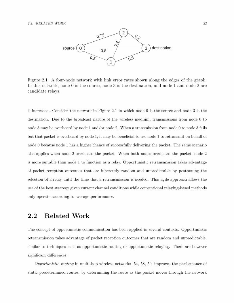
1

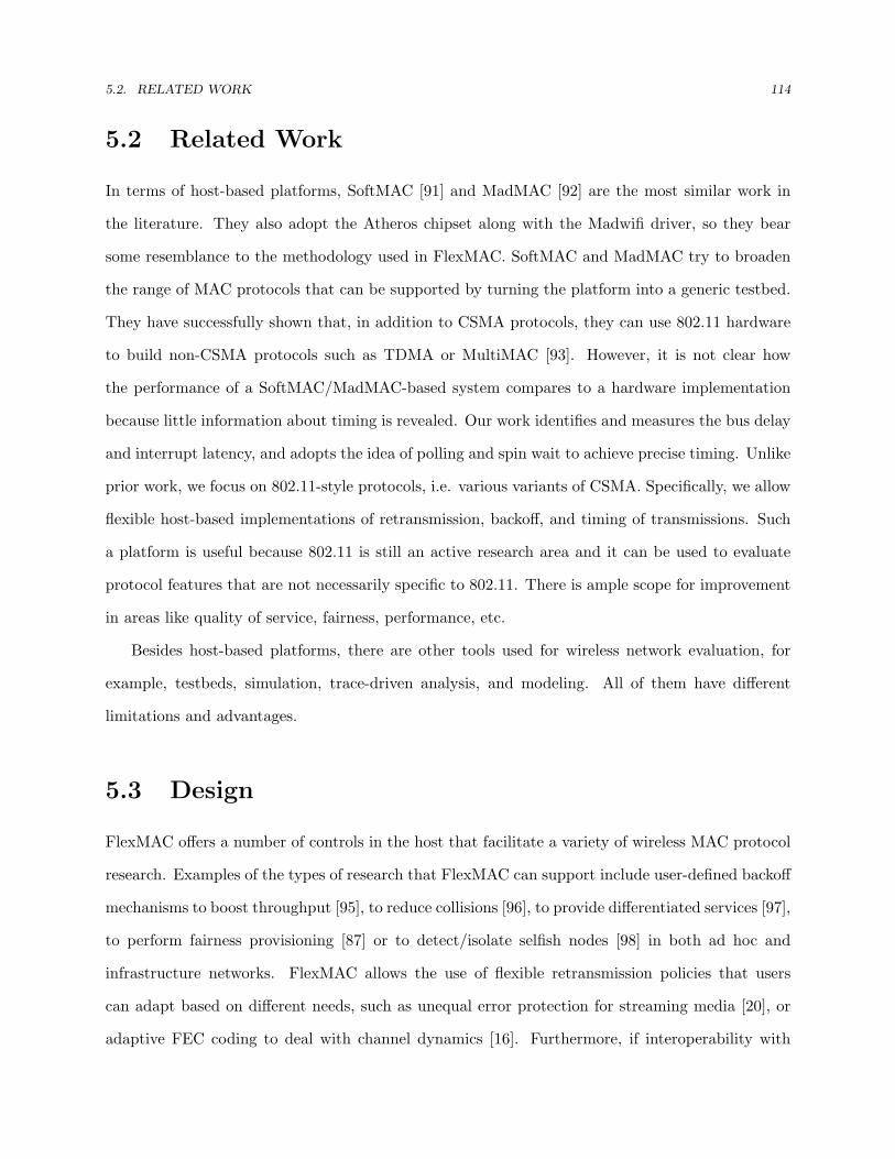
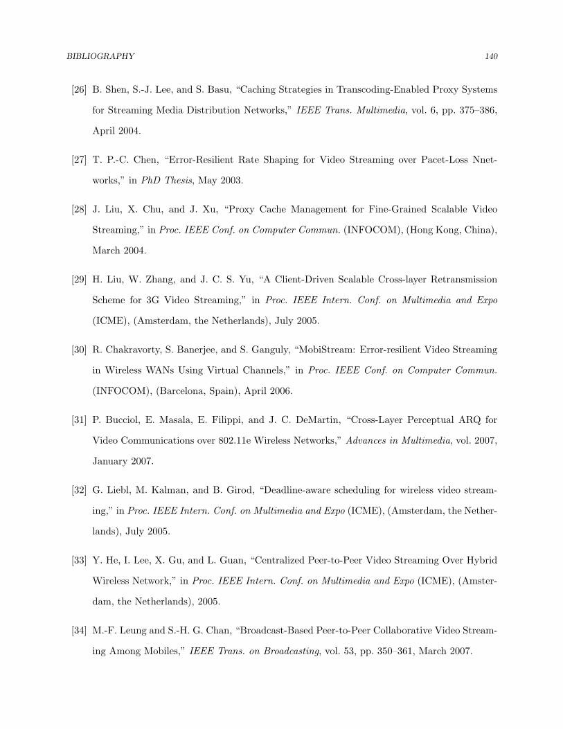
Figure 2.1: A four-node network with link error rates shown along the edges of the graph.In this network, node 0 is the source, node 3 is the destination, and node 1 and node 2 arecandidate relays.

is increased. Consider the network in Figure 2.1 in which node 0 is the source and node 3 is the

destination. Due to the broadcast nature of the wireless medium, transmissions from node 0 to

node 3 may be overheard by node 1 and/or node 2. When a transmission from node 0 to node 3 fails

but that packet is overheard by node 1, it may be beneficial to use node 1 to retransmit on behalf of

node 0 because node 1 has a higher chance of successfully delivering the packet. The same scenario

also applies when node 2 overheard the packet. When both nodes overheard the packet, node 2

is more suitable than node 1 to function as a relay. Opportunistic retransmission takes advantage

of packet reception outcomes that are inherently random and unpredictable by postponing the

selection of a relay until the time that a retransmission is needed. This agile approach allows the

use of the best strategy given current channel conditions while conventional relaying-based methods

only operate according to average performance.

2.2 Related Work

The concept of opportunistic communication has been applied in several contexts. Opportunistic

retransmission takes advantage of packet reception outcomes that are random and unpredictable,

similar to techniques such as opportunistic routing or opportunistic relaying. There are however

significant differences:

Opportunistic routing in multi-hop wireless networks [54, 58, 59] improves the performance of

static predetermined routes, by determining the route as the packet moves through the network


based on which nodes receive each transmission. The actual forwarding is done by the node clos-

est to the destination. While opportunistic retransmission and opportunistic routing bear some

similarity (i.e. exploiting multiple paths between the source and the destination), they are very

different approaches. First, opportunistic retransmission applies to infrastructure mode networks,

so it is more generally applicable. Second, opportunistic routing requires a separate mechanism to

propagate route information. Third, opportunistic routing is forced to use broadcast transmissions

in order to enable receptions at multiple routers because it operates in the network layer. This

constraint raises two issues. One, broadcasts messages are transmitted with basic rates in the link

layer, which can be overly conservative when destinations are nearby. Two, additional gains of

combining rate adaptation are not available. In contrast, opportunistic retransmission is a link

layer technique, so it automatically avoids these overheads. Finally, opportunistic retransmission

does not affect (or may even decrease) packet latency and packet delivery order, while opportunis-

tic routing often does increase latency and generate out-of-order deliveries in order to spread out

scheduling and routing overheads. The increased delay is a problem for interactive applications.

Recently, opportunistic relaying has been proposed as a practical scheme for cooperative diver-

sity, in view of the fact that practical space-time codes for cooperative relay channels are still an

open and challenging area of research [60, 61]. opportunistic relaying relies on a set of cooperating

relays which are willing to forward received information toward the destination. The challenge is

to develop a protocol that selects the most appropriate relay to forward information toward the re-

ceiver. The scheme can be either digital relaying (decode and forward) or analog relaying (amplify

and forward).

Opportunistic retransmission only uses relays that can fully decode the packets. From a func-

tional perspective, opportunistic retransmission can be categorized as a light-weight, decode-and-

forward opportunistic relaying mechanism. It however differs from opportunistic relaying in two

aspects. First, in PRO, the destination does not combine the signals from the source and the relay,

but tries to decode the information using either the direct signal or the relayed signal (in case that

the direct signal is not decodable). This sacrifices some achievable rates but avoids the cost of ad-

ditional receive hardware, so it is easy to deploy. Second, existing opportunistic relaying protocols

2.3. ANALYSIS 24

require RTS/CTS handshake to assess instantaneous link condition and/or to carry the feedback

of relay selection results [60]. RTS/CTS handshake is rarely used because of its inefficiency in

terms of extra bandwidth and delay. PRO avoids such overhead by using the RSSI history and by

leveraging channel reciprocity for link quality estimation as will be explained later in this chapter.

2.3 Analysis

We now study the analytical performance of opportunistic retransmission. For simplicity, the follow-

ing analysis assumes zero overhead and error free feedback. With the assumption of a memoryless

packet erasure channel such that packets are dropped independently with a constant probability,

we can model opportunistic retransmission as a discrete-time Markov chain with time-homogeneous

transition probabilities. Consider an N -node network with source labeled as 0, destination labeled

as N − 1, and N − 2 candidate relays labeled as 1, 2, · · · , N − 2. Let Pmn denote the link error rate

from node m to node n. The system state S = (bin bN−1bN−2 · · · b1) where bi = {0, 1} is defined

as an (N − 1)-bit number with the n-th bit bn representing the packet reception state of node n (1

is successful reception and 0 is a miss). For example, the four-node network in Figure 2.1 contains

a source (node 0), a destination (node 3), and two relays (node 2 and node 3). State 1 = (bin

001) represents node 1 has received the packet but node 2 and node 3 have not. State 2 = (bin

010) represents node 2 has received the packet but node 1 and node 3 have not. States with the

left-most bit bN−1 set indicate successful deliveries to the destination and to simplify the model,

they are grouped into one single state, state 2N−2. Table 2.1 shows the system states of the network

in Figure 2.1. The resulting model is then a (2N−2 + 1)-state Markov chain.

The system starts at state 0 when the source is ready to send a new packet. Every state

transition is a (re)transmission of the packet. The (re)transmission process terminates at state

2N−2 which indicates the destination has successfully received the packet. Hence the goal of this

analysis is to find the expected number of state transitions going from the initial state 0 to the

sink state 2N−2, that is, the average number of (re)transmissions needed to successfully deliver a

packet.

2.3. ANALYSIS 25

Binary Packet Reception StateState Expression Node 1 Node 2 Node 3

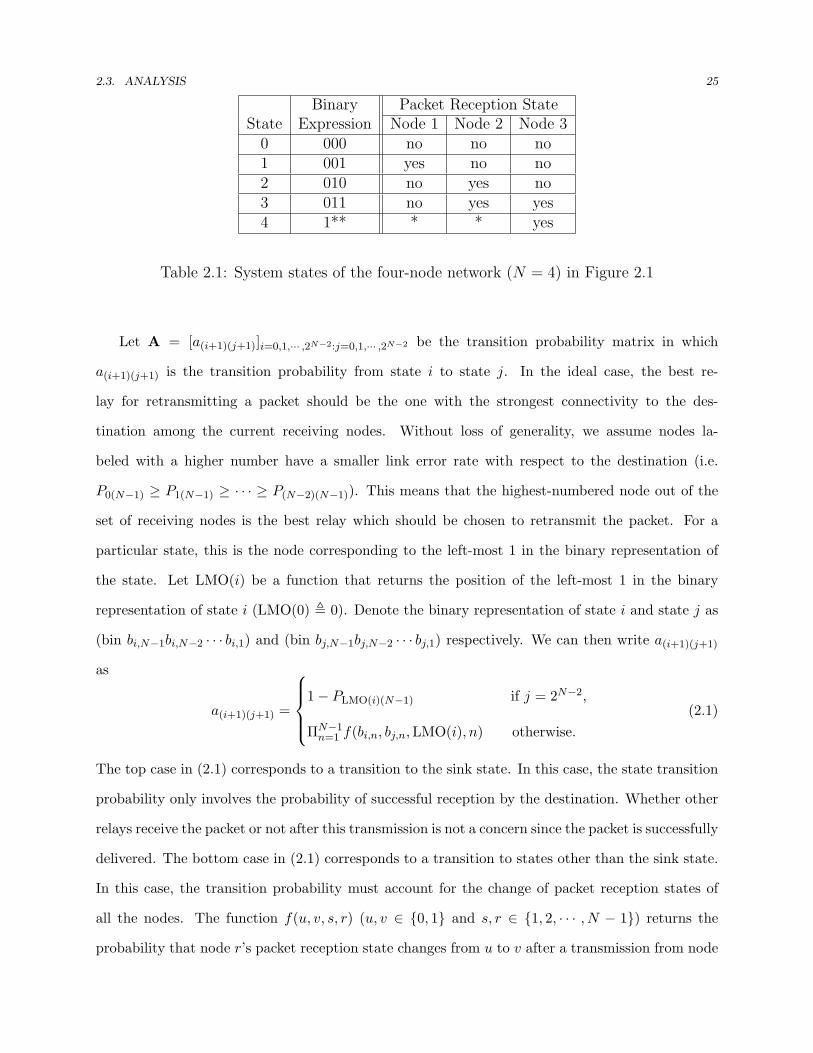
0 000 no no no1 001 yes no no2 010 no yes no3 011 no yes yes4 1** * * yes

Table 2.1: System states of the four-node network (N = 4) in Figure 2.1

Let A = [a(i+1)(j+1)]i=0,1,··· ,2N−2:j=0,1,··· ,2N−2 be the transition probability matrix in which

a(i+1)(j+1) is the transition probability from state i to state j. In the ideal case, the best re-

lay for retransmitting a packet should be the one with the strongest connectivity to the des-

tination among the current receiving nodes. Without loss of generality, we assume nodes la-

beled with a higher number have a smaller link error rate with respect to the destination (i.e.

P0(N−1) ≥ P1(N−1) ≥ · · · ≥ P(N−2)(N−1)). This means that the highest-numbered node out of the

set of receiving nodes is the best relay which should be chosen to retransmit the packet. For a

particular state, this is the node corresponding to the left-most 1 in the binary representation of

the state. Let LMO(i) be a function that returns the position of the left-most 1 in the binary

representation of state i (LMO(0) , 0). Denote the binary representation of state i and state j as

(bin bi,N−1bi,N−2 · · · bi,1) and (bin bj,N−1bj,N−2 · · · bj,1) respectively. We can then write a(i+1)(j+1)

as

a(i+1)(j+1) =

1− PLMO(i)(N−1) if j = 2N−2,

ΠN−1n=1 f(bi,n, bj,n,LMO(i), n) otherwise.

(2.1)

The top case in (2.1) corresponds to a transition to the sink state. In this case, the state transition

probability only involves the probability of successful reception by the destination. Whether other

relays receive the packet or not after this transmission is not a concern since the packet is successfully

delivered. The bottom case in (2.1) corresponds to a transition to states other than the sink state.

In this case, the transition probability must account for the change of packet reception states of

all the nodes. The function f(u, v, s, r) (u, v ∈ {0, 1} and s, r ∈ {1, 2, · · · , N − 1}) returns the

probability that node r’s packet reception state changes from u to v after a transmission from node

2.3. ANALYSIS 26

OR: State Transition Matrix (Revised)

030201 PPP

4

1312 PP 1

03P

030201 PPP

13P

1 32

030201 PPP030201 PPP

0312 PP2321 PP

2321 PP23P

23P

23P0

⎥⎥⎥⎥⎥⎥

⎦

⎤

⎢⎢⎢⎢⎢⎢

⎣

⎡

=

100000000000

23231303

2323211312030201

2321030201

1312030201

030201

PPPPPPPPPPPP

PPPPPPPPPP

PPP

A

Notation: pp −=1

Assume smaller numbered nodes locate closer to the destination, i.e.

231303 PPP <<

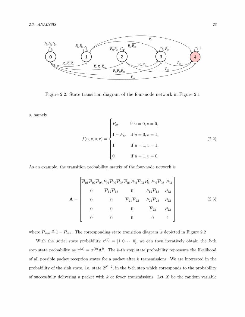
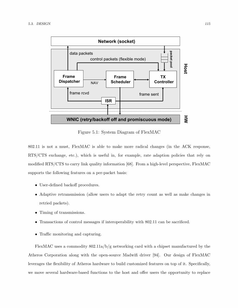
Figure 2.2: State transition diagram of the four-node network in Figure 2.1

s, namely

f(u, v, s, r) =

Psr if u = 0, v = 0,

1− Psr if u = 0, v = 1,

1 if u = 1, v = 1,

0 if u = 1, v = 0.

(2.2)

As an example, the transition probability matrix of the four-node network is

A =

P 01P 02P 03P01P 02P 03P 01P02P 03P01P02P 03 P03

0 P 12P 13 0 P12P 13 P13

0 0 P 21P 23 P21P 23 P23

0 0 0 P 23 P23

0 0 0 0 1

(2.3)

where Pmn , 1− Pmn. The corresponding state transition diagram is depicted in Figure 2.2

With the initial state probability π(0) = [1 0 · · · 0], we can then iteratively obtain the k-th

step state probability as π(k) = π(0)Ak. The k-th step state probability represents the likelihood

of all possible packet reception states for a packet after k transmissions. We are interested in the

probability of the sink state, i.e. state 2N−2, in the k-th step which corresponds to the probability

of successfully delivering a packet with k or fewer transmissions. Let X be the random variable

2.3. ANALYSIS 27

representing the number of transmissions needed to successfully deliver a packet. We then get

π(k)

2N−2 = Pr(X ≤ k) (2.4)

which is the cumulative distribution function (CDF) of X. Thus the average number of transmis-

sions needed to deliver a packet by opportunistic retransmission can be obtained as

E[X] =∞∑

k=1

k · (Pr(X ≤ k)− Pr(X ≤ k − 1)) =∞∑

k=1

k · (π(k)

2N−2 − π(k−1)

2N−2 ). (2.5)

If we view the source and relays jointly as a sending system and the network as a transmission

system that connects the sending system to the destination, the packet error rate (i.e., the reciprocal

of the number of transmissions associated with the packet) can be written as

Pe = 1− 1E[X]

. (2.6)

Next we consider a mesh network-based approach for performance comparison. Mesh network-

based approaches use the least-cost multi-hop path to forward packets. Thus the optimal multi-hop

path has the minimum number of transmissions, that is,

TX∗mesh net = min

l(∑`∈l

1P`

) (2.7)

where ` is a composing link in a path l and P` is the link delivery rate. The overall packet error

rate for mesh networking is then

Pe = 1− 1TX∗

mesh net

. (2.8)

Using the above analysis, we compare opportunistic retransmission with the mesh network-

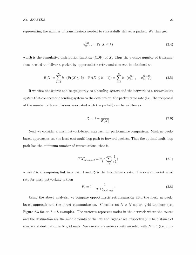
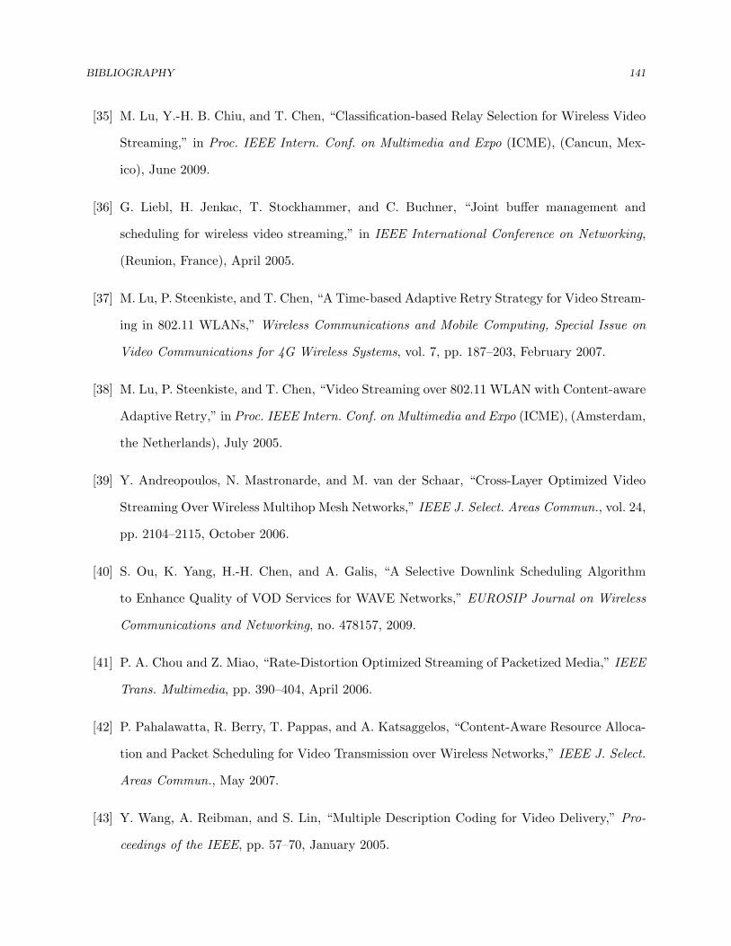
based approach and the direct communication. Consider an N × N square grid topology (see

Figure 2.3 for an 8 × 8 example). The vertexes represent nodes in the network where the source

and the destination are the middle points of the left and right edges, respectively. The distance of

source and destination is N grid units. We associate a network with no relay with N = 1 (i.e., only

2.3. ANALYSIS 28

0 0.25 0.5 0.75 10

0.25

0.5

0.75

1

source destination

Figure 2.3: Network with an 8× 8 square grid topology.

0.4

0.5

0.6

0.7

0.8

0.9

1

0 1 2 3 4 5Network density (log2N)

Pac

ket L

oss

Rat

e

Opport. Retx Mesh NetDirect Comm.

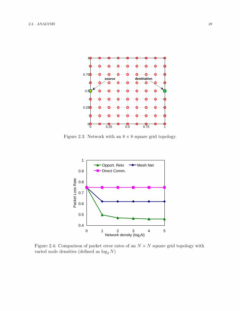
Figure 2.4: Comparison of packet error rates of an N ×N square grid topology withvaried node densities (defined as log2 N)

2.4. PROTOCOL DESIGN 29

Monitor LQ from all overheard

packets

Per nodeLQ history

Overhear a failed data packet

Yes

Relay the packet based on

prioritization

Retransmission

Periodically advertise local LQ

to the network

Background

Decide the set of eligible relays

Receive LQ info from other relays

Am I a qualified

relay?

Am Ian eligible

relay?

Yes

Figure 2.5: Protocol flowchart of PRO

the source and the destination are present in the network). Assume link error rate Pij from node i

to node j is a function of node distance dij with path loss exponent 1.6. We define Pij as

Pij(dij) = 1− Psd

dij1.6 (2.9)

where dij is the node distance in grid units and Psd is the link error rate from the source to the

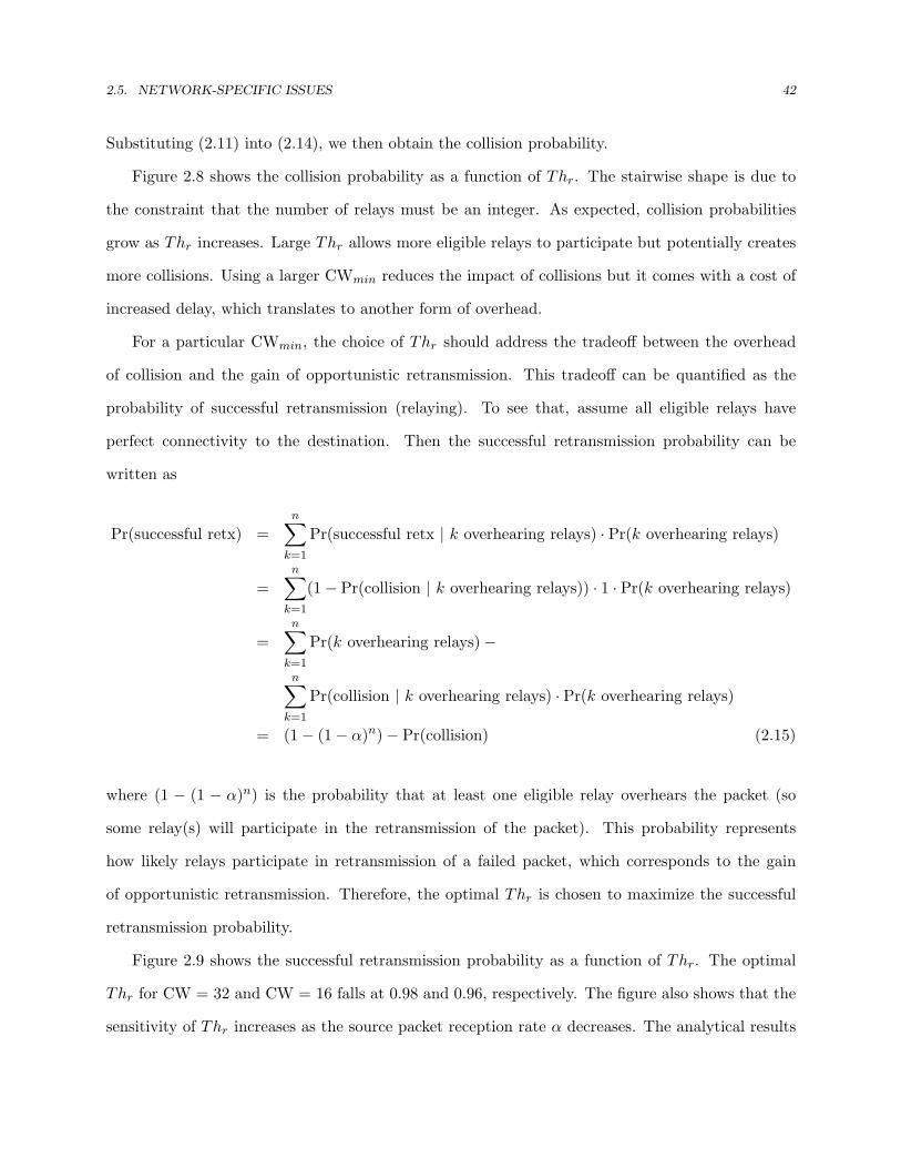
destination. Figure 2.4 shows the analytical comparison results for square grid topologies with dif-

ferent N . The source-destination link error rate, Psd is 0.75. The figure indicates that opportunistic

retransmission outperforms the optimal mesh network-based approach which in turn outperforms

direct communication. Moreover, while the performance eventually saturates, opportunistic re-

transmission exhibits increased gains as more nodes are present.

2.4 Protocol Design

The analysis presented in the previous section demonstrates the theoretical gain of opportunistic

retransmission when protocol overheads are neglected. To investigate the effectiveness of oppor-


tunistic retransmission in practice, we have designed and developed an efficient opportunistic re-

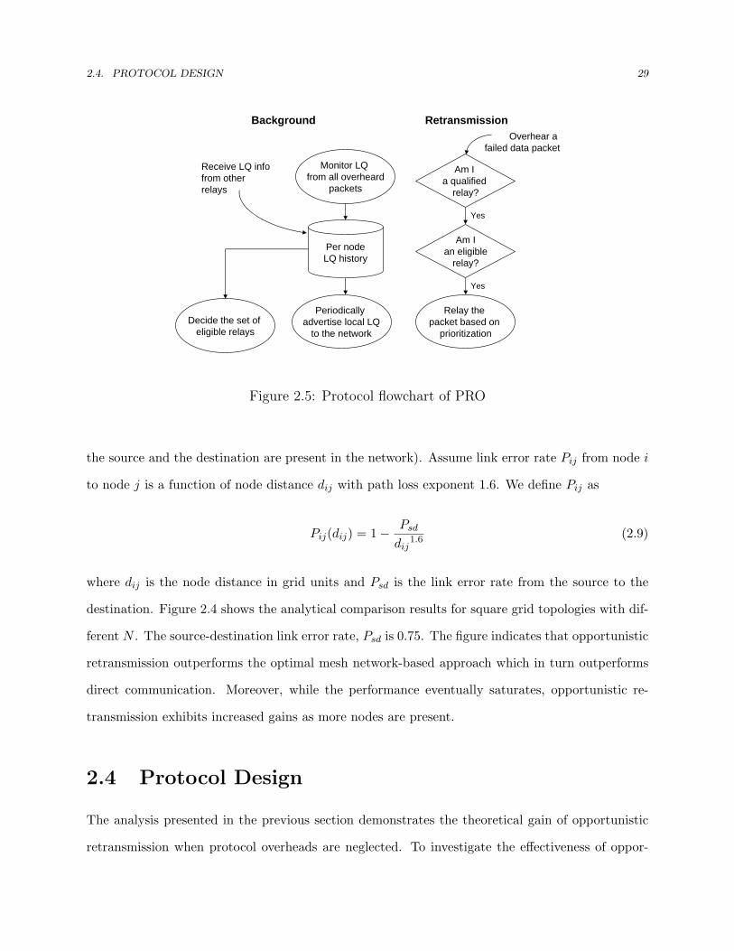
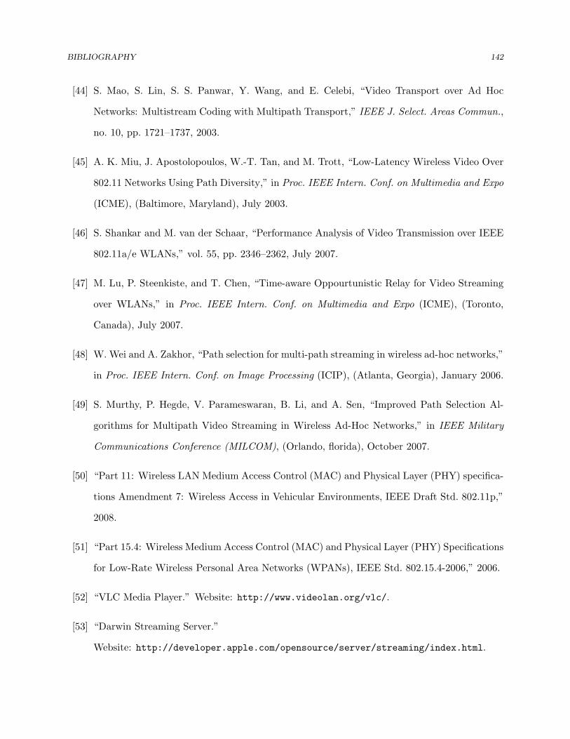
transmission protocol (PRO, Protocol for Retransmission Opportunistically). Figure 2.5 gives an

overview of PRO. In the background, candidate relays continuously monitor the link quality with

respect to the source(s) and the destination(s). The channel quality to the destination shows how

likely the node can successfully (re)transmit packets to the destination. The channel quality to the

source indicates how often the node is likely to overhear packets from the source, i.e. how often

the node will be in a position to function as a relay to the destination. Each node locally decides

whether it is a qualified relay for a source-destination pair based on a threshold for the quality of

the channel to the destination. Qualified relays advertise their link quality with respect to both

the source and the destination through periodic broadcasts.

By collecting periodic link quality broadcasts, each qualified relay independently constructs a

global map of the connectivity between qualified relays, the source, and the destination. Using this

information, each qualified relay then decides whether it is an eligible relay for a destination. Only

eligible relays are allowed to retransmit after a failed transmission. Clearly, the selection process

should result in a set of eligible relays that is large enough so there is a high likelihood that one

of them overhears the source. On the other hand, including too many relays can be harmful for

several reasons. First, using too many relays can potentially increase contention in the network

which may result in more collisions. Second, having poorer relays retransmit prevents (or delays)

retransmission by better relays, thus reducing the success rate for retransmissions.

When eligible relays overhear a data packet without followed by an corresponding ACK1, they

participate in the retransmission of the packet. For random access wireless networks like 802.11

WLANs, the opportunistic retransmission process leverages the standard random access procedure.

This is the same as retransmitting a local packet. Relays stop the retransmission when they overhear

an acknowledgement that confirms a successful reception by the receiver. To give precedence to

relays with better connectivity to the destination, eligible relays choose the size of initial contention

window based on their priority i.e. their rank in terms of how effective they are among all eligible

1In the 802.11 standard, destinations send an ACK message after successfully receiving a data packet in aSIFS interval to indicate a successful reception. So sources (and relays) can conjecture a failed transmissionfrom a missing ACK.


relays. Relays with a higher rank are associated with a smaller contention window so that they have

a higher chance of accessing the channel. For other types of wireless networks, relay prioritization

can be performed in a contention period following the contention free period. We elaborate on each

functional component in the following subsections.

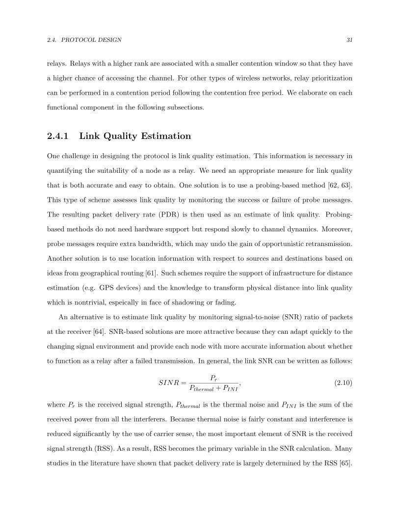
2.4.1 Link Quality Estimation

One challenge in designing the protocol is link quality estimation. This information is necessary in

quantifying the suitability of a node as a relay. We need an appropriate measure for link quality

that is both accurate and easy to obtain. One solution is to use a probing-based method [62, 63].

This type of scheme assesses link quality by monitoring the success or failure of probe messages.

The resulting packet delivery rate (PDR) is then used as an estimate of link quality. Probing-

based methods do not need hardware support but respond slowly to channel dynamics. Moreover,

probe messages require extra bandwidth, which may undo the gain of opportunistic retransmission.

Another solution is to use location information with respect to sources and destinations based on

ideas from geographical routing [61]. Such schemes require the support of infrastructure for distance

estimation (e.g. GPS devices) and the knowledge to transform physical distance into link quality

which is nontrivial, espeically in face of shadowing or fading.

An alternative is to estimate link quality by monitoring signal-to-noise (SNR) ratio of packets

at the receiver [64]. SNR-based solutions are more attractive because they can adapt quickly to the

changing signal environment and provide each node with more accurate information about whether

to function as a relay after a failed transmission. In general, the link SNR can be written as follows:

SINR =Pr

Pthermal + PINI, (2.10)

where Pr is the received signal strength, Pthermal is the thermal noise and PINI is the sum of the

received power from all the interferers. Because thermal noise is fairly constant and interference is

reduced significantly by the use of carrier sense, the most important element of SNR is the received

signal strength (RSS). As a result, RSS becomes the primary variable in the SNR calculation. Many

studies in the literature have shown that packet delivery rate is largely determined by the RSS [65].


1472 bytes

0

0.2

0.4

0.6

0.8

1

4 6 8 10 12 14 16

RSSI

Pac

ket D

eliv

ery

Rat

io

Pair 1Pair 2

(a) 1472 bytes

1024 bytes

0

0.2

0.4

0.6

0.8

1

4 6 8 10 12 14 16

RSSI

Pac

ket D

eliv

ery

Rat

io

Pair 1Pair 2

(b) 1024 bytes

512 bytes

0

0.2

0.4

0.6

0.8

1

4 6 8 10 12 14 16

RSSI

Pac

ket D

eliv

ery

Rat

io

Pair 1Pair 2

(c) 512 bytes

16 bytes

0

0.2

0.4

0.6

0.8

1

4 6 8 10 12 14 16

RSSI

Pac

ket D

eliv

ery

Rat

io

Pair 1Pair 2

(d) 16 bytes

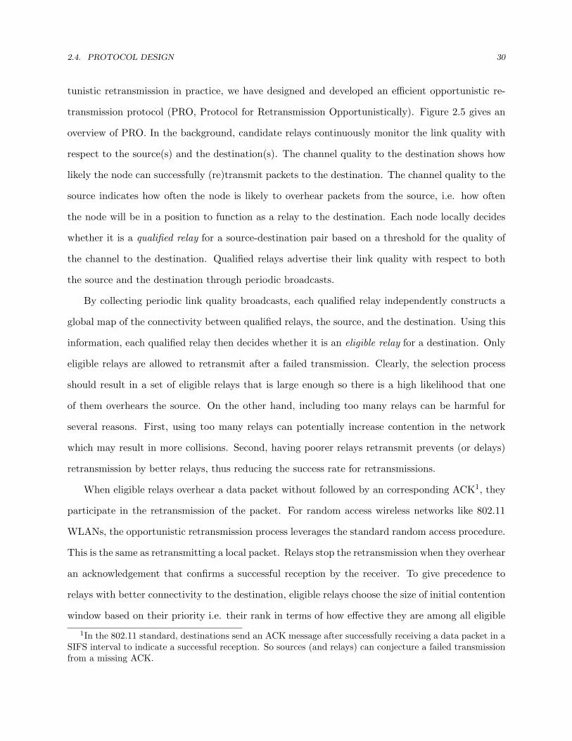
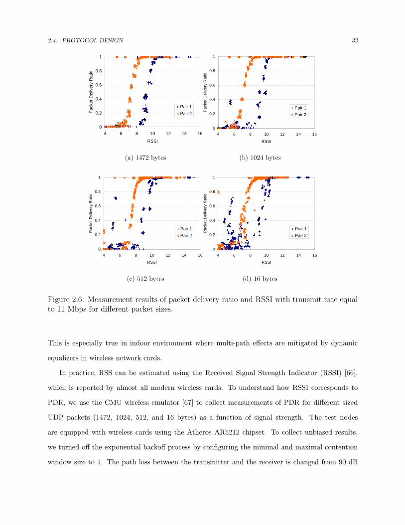
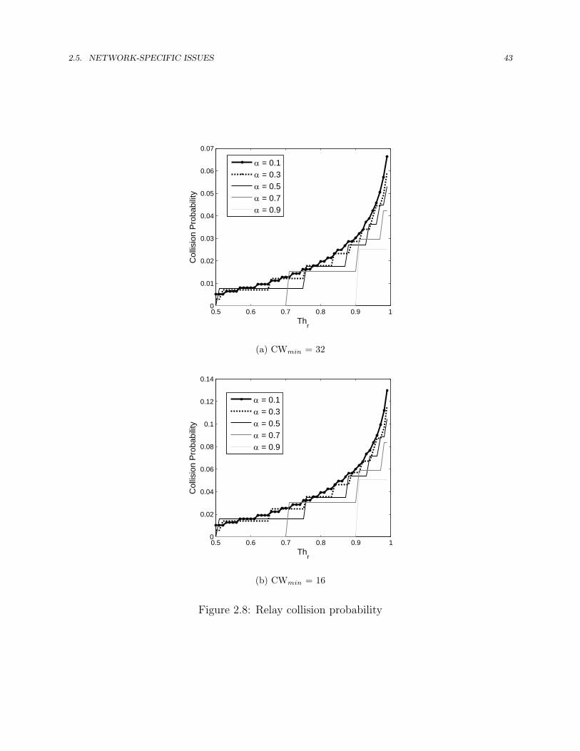
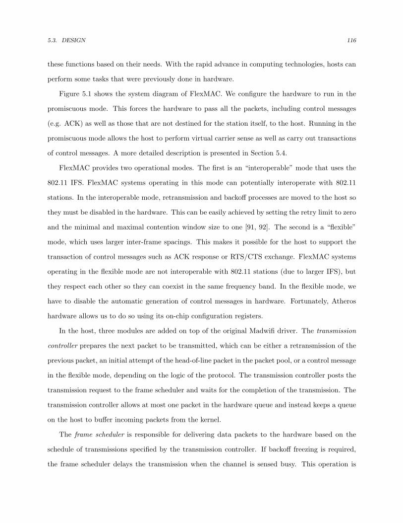
Figure 2.6: Measurement results of packet delivery ratio and RSSI with transmit rate equalto 11 Mbps for different packet sizes.

This is especially true in indoor environment where multi-path effects are mitigated by dynamic

equalizers in wireless network cards.

In practice, RSS can be estimated using the Received Signal Strength Indicator (RSSI) [66],

which is reported by almost all modern wireless cards. To understand how RSSI corresponds to

PDR, we use the CMU wireless emulator [67] to collect measurements of PDR for different sized

UDP packets (1472, 1024, 512, and 16 bytes) as a function of signal strength. The test nodes

are equipped with wireless cards using the Atheros AR5212 chipset. To collect unbiased results,

we turned off the exponential backoff process by configuring the minimal and maximal contention

window size to 1. The path loss between the transmitter and the receiver is changed from 90 dB


to 110 dB with a step size of 0.5 dB. For a particular loss value, we collected average RSSI and

PDR over 1000 packets and repeated the test 10 times. Figure 2.6 shows the measurement results

of average PDR and RSSI for two transmitter/receiver pairs (out of 10 pairs in total). The other

eight pairs exhibit similar behavior. We make the following observations based on these results:

1. PDR as function a of RSSI is somewhat noisy, in particular for 16-byte UDP packets. How-

ever, there is still strong correlation between RSSI and PDR.

2. There is a RSSI high threshold (Thh), above which packets are nearly always received.

3. For different hardware, PDR-RSSI relationship exhibits a similar shape with a shift of 2 ∼ 4

dB. With channel reciprocity, forward link quality can be predicted by reverse link conditions

if the amount of shift is known.

Similar observations are also made in other papers [66]. These results suggests that RSSI is not a

perfect measure for PDR, but as we will show later it suffices for our needs. PRO does not require

a very accurate measure of link quality because link quality is used to help select and prioritize

a reasonable set of relays from a larger pool, and small changes in quality should not affect this

process. In the next subsection, we describe how we leverage the above observations to design an

efficient opportunistic retransmission protocol.

In practice, channel conditions vary with time. To predict the current RSSI, PRO uses the

RSSI history of packets with the time-aware prediction algorithm proposed in [57]. This approach

improves exponential weighted moving average (EWMA) by weighing recent samples more and

filtering out sharp transient fades that last for only a single packet.

2.4.2 Relay Qualification

Using too many or poor relays can hurt performance since it increases the probability of collisions

while offering limited opportunistic gains. To filter out poor relays early, candidate nodes must

pass a qualification process by comparing the RSSI with respect to the destination with threshold

Thh. Qualified relays periodically broadcast their link quality with respect to the source and


the destination to the network. This information is then used for relay selection, which will be

elaborated in Section 2.4.3.

The qualification process involves one challenge: using the reverse link condition to predict

forward link quality is imprecise if links are asymmetric. Unfortunately, conveying RSSI information

from the destination to the relay using e.g. RTS/CTS handshake [64, 68] introduces relatively high

overheads that can easily undo any performance benefits. PRO avoids such overheads by leveraging

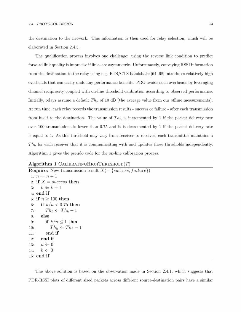
channel reciprocity coupled with on-line threshold calibration according to observed performance.

Initially, relays assume a default Thh of 10 dB (the average value from our offline measurements).

At run time, each relay records the transmission results - success or failure - after each transmission

from itself to the destination. The value of Thh is incremented by 1 if the packet delivery rate

over 100 transmissions is lower than 0.75 and it is decremented by 1 if the packet delivery rate

is equal to 1. As this threshold may vary from receiver to receiver, each transmitter maintains a

Thh for each receiver that it is communicating with and updates these thresholds independently.

Algorithm 1 gives the pseudo code for the on-line calibration process.

Algorithm 1 CalibratingHighThreshold(T )

Require: New transmission result X(= {success, failure})1: n ⇐ n + 12: if X = success then3: k ⇐ k + 14: end if5: if n ≥ 100 then6: if k/n < 0.75 then7: Thh ⇐ Thh + 18: else9: if k/n ≤ 1 then

10: Thh ⇐ Thh − 111: end if12: end if13: n ⇐ 014: k ⇐ 015: end if

The above solution is based on the observation made in Section 2.4.1, which suggests that

PDR-RSSI plots of different sized packets across different source-destination pairs have a similar


shape. Note that our calibration process does not need to consider the reason for the packet losses,

making it agile to deal with various conditions. For example, if packet losses are due to a jammer on

the path between the relay and the destination, then the calibration process gradually increments

Thh, making the relay less and less likely to pass the relay qualification process. The calibration

process resets Thh to the default value if no transmission to the destination occurs during the

past 30 minutes to compensate for threshold adjustment due to the environment, not due to card

characteristics.

2.4.3 Relay Selection

Relay selection finds the best set of relay(s) among all candidates to retransmit packets in error. Ef-

fective relay selection should increase the probability of successful retransmission while minimizing

collisions and duplicate packets. To assure that overhead does not overwhelm gains, PRO uses a

distributed relay selection algorithm. Each qualified relay runs the algorithm to find a set of eligible

relays out of all the qualified relays based on their link quality with respect to the source and the

destination. A qualified relay then identifies itself as an eligible relay if it falls into the selected

set. Upon a failed transmission, eligible relays that overheard the packet attempt to transmit the

packet. Eligible relays are prioritized based on their relaying performance. This is achieved by

using a smaller contention window for high priority relays.

In the subsequent subsection, we elaborate on how relays share link quality information with

each other and how the relay selection algorithm works. The details of relay prioritization will be

addressed in Section 2.4.4.

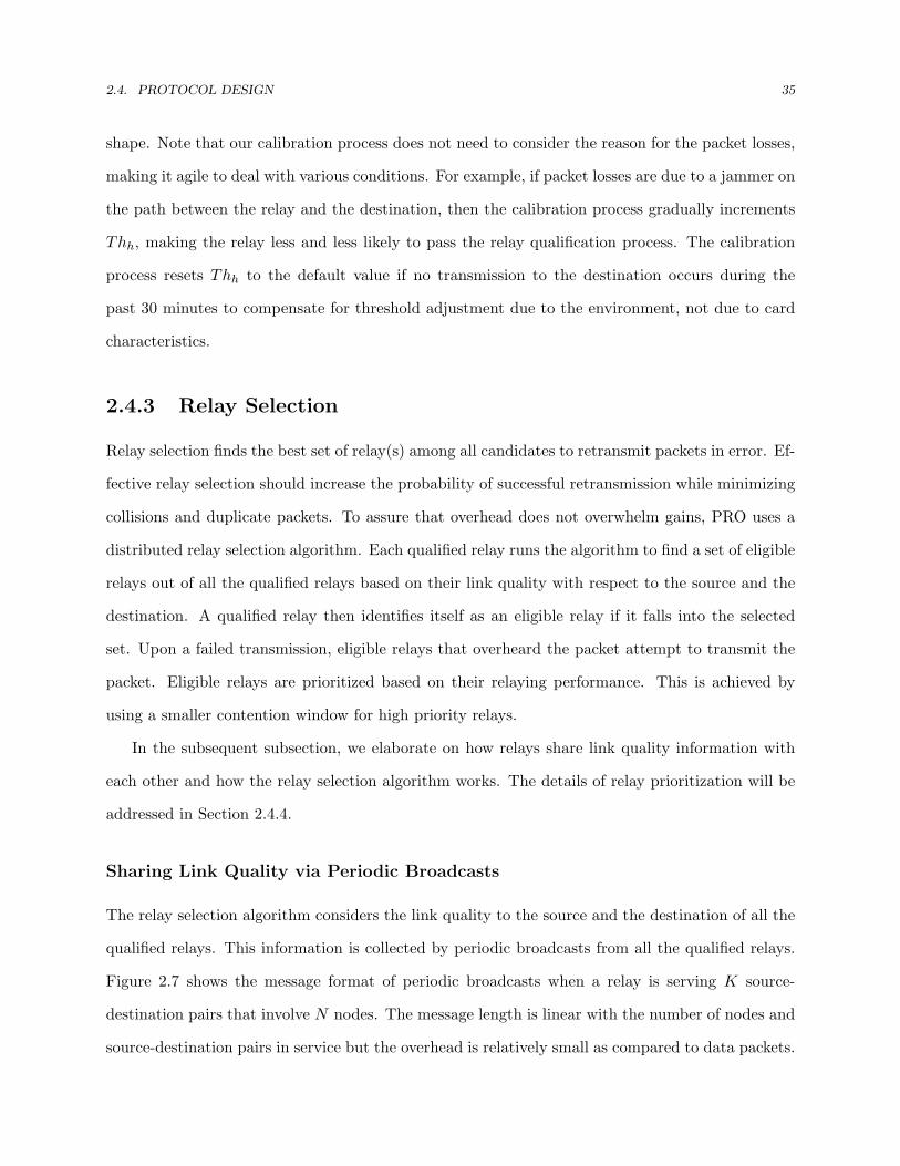
Sharing Link Quality via Periodic Broadcasts

The relay selection algorithm considers the link quality to the source and the destination of all the

qualified relays. This information is collected by periodic broadcasts from all the qualified relays.

Figure 2.7 shows the message format of periodic broadcasts when a relay is serving K source-

destination pairs that involve N nodes. The message length is linear with the number of nodes and

source-destination pairs in service but the overhead is relatively small as compared to data packets.


Frame control

Dur-ation

Address1

Address 2

Address 3 Seq. Address

4Check-

sumPeriodic Broadcast

Message Body

Bytes 2 2 6 6 6 2 6 4

control ation 1 2 3 4 sumMessage Body

N d 1 N d NP i 1 P i 1 P i K P i K

Bytes 1 1 1 1 1 2 2

Node1LQ … NodeN

LQPair1

Src_IDPair1

Dst_IDPairK

Src_IDPairK

Dst_ID… 0x0

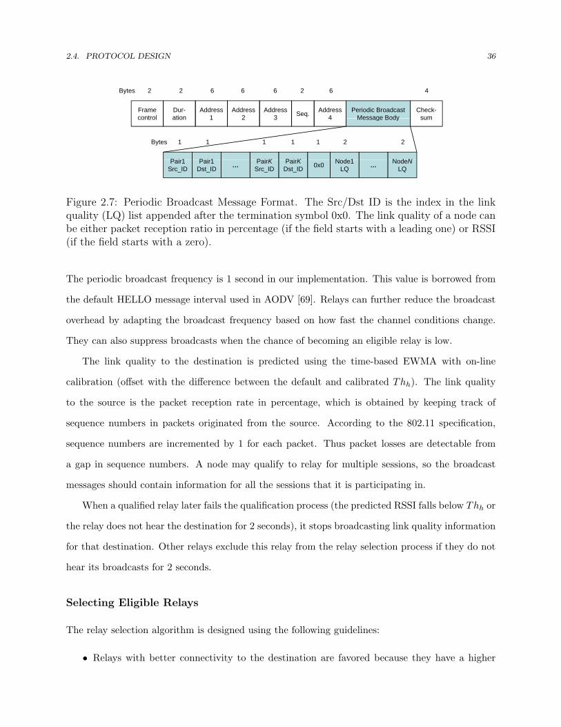
Figure 2.7: Periodic Broadcast Message Format. The Src/Dst ID is the index in the linkquality (LQ) list appended after the termination symbol 0x0. The link quality of a node canbe either packet reception ratio in percentage (if the field starts with a leading one) or RSSI(if the field starts with a zero).

The periodic broadcast frequency is 1 second in our implementation. This value is borrowed from

the default HELLO message interval used in AODV [69]. Relays can further reduce the broadcast

overhead by adapting the broadcast frequency based on how fast the channel conditions change.

They can also suppress broadcasts when the chance of becoming an eligible relay is low.

The link quality to the destination is predicted using the time-based EWMA with on-line

calibration (offset with the difference between the default and calibrated Thh). The link quality

to the source is the packet reception rate in percentage, which is obtained by keeping track of

sequence numbers in packets originated from the source. According to the 802.11 specification,

sequence numbers are incremented by 1 for each packet. Thus packet losses are detectable from

a gap in sequence numbers. A node may qualify to relay for multiple sessions, so the broadcast

messages should contain information for all the sessions that it is participating in.

When a qualified relay later fails the qualification process (the predicted RSSI falls below Thh or

the relay does not hear the destination for 2 seconds), it stops broadcasting link quality information

for that destination. Other relays exclude this relay from the relay selection process if they do not

hear its broadcasts for 2 seconds.

Selecting Eligible Relays

The relay selection algorithm is designed using the following guidelines:

• Relays with better connectivity to the destination are favored because they have a higher


chance to successfully transmit the packet.

• Relays with better connectivity to the source are favored because they have a high likelihood

to overhear the source and offer opportunistic gains.

• The resulting set must be large enough so there is a high likelihood that at least one of

them overhears the source and on the other hand, small enough to minimize collisions while

creating sufficient retransmission opportunities.

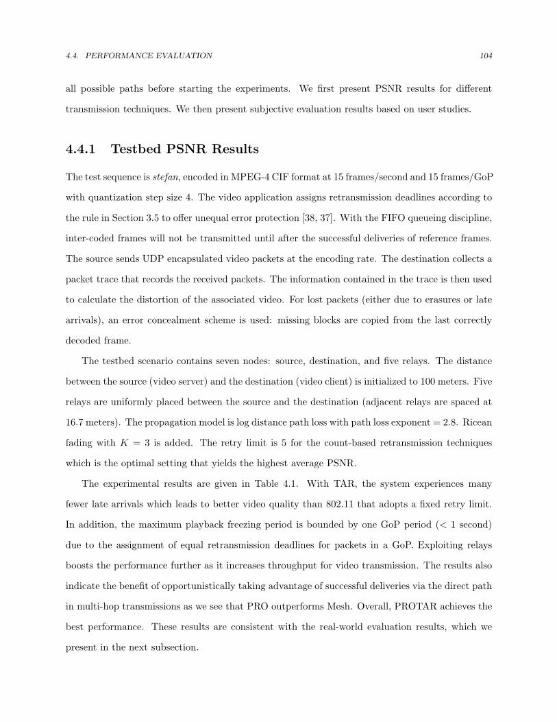
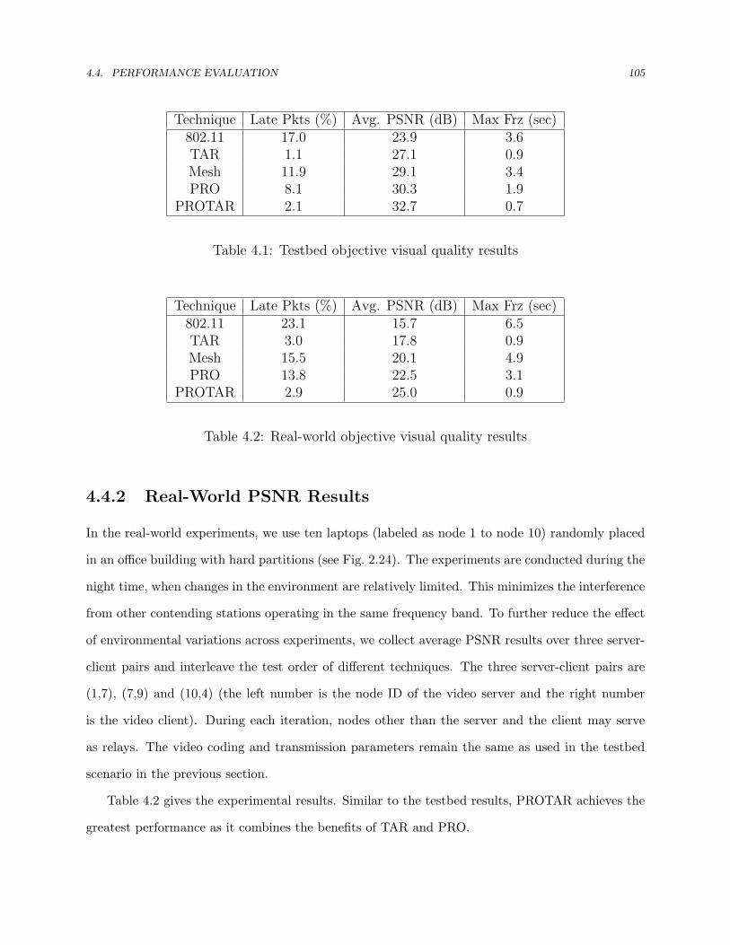
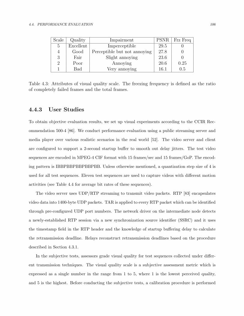
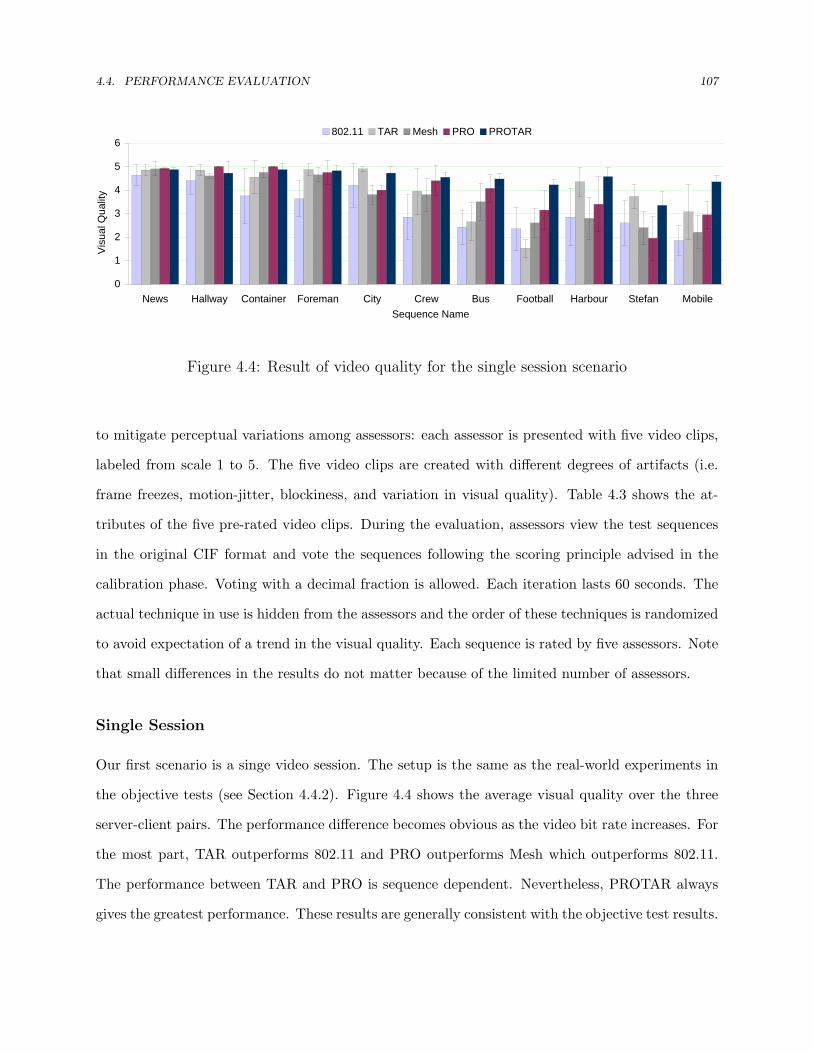
The algorithm works as follows. The selection starts with the node that has the highest RSSI

with respect to the destination and continues adding the next higher node until the probability of

having one of the selected relays hear the source is large enough, i.e. larger than a threshold Thr.

Since source packet reception rates are used to select the right number of participating nodes, the

estimation does not have to be very accurate. Experimental results in Section 2.6 show that our

relay selection algorithm works very well. The psuedo code for the algorithm is given in Algorithm 2.

Algorithm 2 RelaySelection(Q)

Require: All qualified relays QEnsure: All eligible relays R1: Initialize Q to the set of all qualified relays2: R ⇐ ∅3: p ⇐ 14: Rank Q according to the RSSI with respect to the destination. Break tie according to

the RSSI with respect to the source.5: while Q is not empty do6: Pick the highest ranked q in Q7: Insert q to R and delete q from Q8: Retrieve the source packet reception ratio αq of q9: p ⇐ p · (1− αq)

10: if 1− p > Thr then11: return R12: end if13: end while


2.4.4 Relay Prioritization

At run time, there may be multiple eligible relays overhearing a failed transmission. Performance

can be further improved by giving precedence to relays with high RSSI with respect to the desti-

nation. A straightforward solution is to have relays sending feedback and collecting feedback after

each failed transmission. Based on the feedback, the current best relay can be identified and that

relay is responsible for transmitting the packet [60, 70]. Using feedback has two problems. First, it

requires scheduling among relays to decide who sends feedback when, which introduces additional

complexity. Second, the overhead of distributing feedback for every failed transmission can be

considerable.

To reduce overhead, PRO avoids using feedback on a per-transmission basis and instead lever-

ages the standard random backoff procedure to prioritize the relays. The 802.11 standard provides

several mechanisms for achieving this, e.g. by managing the minimal and maximal contention

window size (CWmin and CWmax), backoff increasing factor, interframe space, and backoff time

distribution [71]. For example, 802.11e EDCA [72] performs prioritization by manipulating inter-

frame space or/and contention window size. In our current implementation, effective relays are

prioritized by a smaller CWmin, but other parameters can be considered. Note that the source

behaves as an eligible relay after a failed transmission. That is, it uses a CWmin determined by

the above scheme for retransmissions.

2.4.5 Retransmission

Relays detect failed transmissions through the lack of an ACK. Eligible relays that overheard the

packet then contend to retransmit the packet using the contention window assigned in the relay

prioritization procedure. If the retransmission fails again, relays double the size of contention

windows, select new backoff intervals, and contend again for the channel. The process on each

relay is the same as retransmitting a local packet. Therefore, retransmissions for a packet are

not necessary from a single relay. When the first retransmission fails again, it is likely that new

eligible relays overhear the packet and join the attempt for the second retransmission (i.e., these

relays did not overhear the initial transmission from the source). Newly-joined relays use initial


contention windows to contend the channel so they will have a higher chance to transmit. We

allow this prejudice because newly-joined relays tend to be further from the source and closer to

the destination.

In our current implementation, relays that have pending local packets do not participate in

relaying. This practice is based on the assumption that nodes are willing to support others only

when they have spare resources to do so. In the future, we will explore different policies that have

nodes act as relays even if they have packets pending. Such policies are useful in e.g., scenarios

with concurrent sessions as we will see in Section 2.6.2.

Relays terminate the retransmission process in response to the following events:

• An ACK frame destined for the source is overheard, since it implies successful reception.

• The retry limit is reached after several unsuccessful transmissions. This is similar to dropping

a local packet that has been retransmitted too many times except that the retry count includes

retransmissions from all the relays.

• A new data packet (i.e. the packet stamped with a larger sequence number) originated from

the source is overheard. This means that either the source has discarded the current packet,

or the packet was successfully received but this relay missed the ACK. In either case, the

relay should stop retransmitting the packet.

• The relay overhears first an ACK and then a retransmission of the packet. This means that

the packet was received successfully, but either a relay or the source did not hear the ACK.

The relay should stop retransmitting the duplicate packet and re-acknowledge it.

In the last case, we need a way of reliably re-acknowledging the packet. The obvious solution,

sending another ACK, does not work: if multiple relays detect the unnecessary retransmission, it

will lead to systematic collisions of the ACKs. Instead, they send a “null” data packet, i.e. the

original data packet with the payload stripped and replaced with acknowledgement information.

Since null packets are transmitted as data packets (i.e. use backoff), we avoid systematic collisions.

Note that when the unnecessary retransmission was sent by the source, this approach effectively

corresponds to retransmission of the ACK.

2.5. NETWORK-SPECIFIC ISSUES 40

When destinations are not within the communication range of the sources, frequent retrans-

mission of ACKs may occur. In that case, it may be more efficient to employ the mesh network

based approach (i.e. sources first send packets to a relay which then forwards them to the des-

tination) as there will be little opportunistic gain (see Section 2.6.2 for experimental results of

such phenomenon). In the subsequent subsection, we present an example source-driven design that

supports dynamic switching between PRO and the mesh network based approach.

2.4.6 Dynamic Switching between PRO and Mesh Networking

In response to frequent relaying of ACKs, the source switches to the mesh networking mode and

notifies relays by marking a flag in the packets. The relay selection algorithm, instead of deciding

a set of relays, finds the best relay to function as the forwarder in a distributed fashion. The best

relay must have a high likelihood of overhearing the transmission from the source as well as a high

probability of successfully forwarding packets to the destination. The forwarder generates an ACK

after successful reception of a packet from the source and forwards the packet to the destination.

The source switches back to the opportunistic retransmission mode later after it starts overhearing

traffic from the destination.

2.5 Network-Specific Issues

In this section we discuss a number of network-specific issues, in particularly, 802.11-based wireless

networks. They are all evaluated in Section 2.6.

2.5.1 Collision Avoidance

The main overhead of PRO is an increased probability of collisions due to transmissions from mul-

tiple relays. Collision avoidance has been partly addressed in the design of PRO’s relay selection

algorithm. The choice of threshold Thr implicitly limits how many eligible relays are selected.

Larger Thr grants more relays, which increases opportunistic gains but potentially creates more

collisions. To understand this tradeoff, this section presents an analytical study of collision proba-


bilities as a function of Thr. The analytical results are then used for selecting a proper Thr. The

study considers an 802.11-like wireless networking environment.

Consider N qualified relays. For simplicity, assume these relays have an equal probability of

hearing the source, denoted as α. Moreover, consider a single priority class that allows all relays to

contend for the channel with the same uniform distribution [0, CW − 1]. This corresponds to the

worse case where the contention level is maximal. The probability function f(x) and the cumulative

mass function F (x) =∑

x f(x) are

f(x) =1

CWand F (x) =

x + 1CW

where x ∈ {0, 1, 2, · · · , CW − 1}. (2.11)

According to the relay selection algorithm, n out of N relays are identified as eligible relays. Given

Thr, n can be derived by

n = arg mini{1− (1− α)i ≥ Thr} = dlog1−α (1− Thr)e. (2.12)

Upon a failed transmission, a subset of eligible relays overhears the packet and contends for the

channel to retransmit the packet. Denote the subset size as k (k ≤ n). Collisions occur when

the lowest-numbered backoff slot selected by the k relays is associated with two or more relays.

Equivalently, the collision probability is one minus the probability that the lowest-numbered backoff

slot is only associated with one relay:

Pr(collision | k overhearing relays) = 1− Pr(successful retx | k overhearing relays)

= 1− k

CW−1∑x=0

f(x)(1− F (x))k−1. (2.13)

According to the law of total probability, we can derive

Pr(collision) =n∑

k=2

Pr(collision | k overhearing relays) · Pr(k overhearing relays)

=n∑

k=2

(1− k

CW−1∑x=0

f(x)(1− F (x))k−1)·

(n

k

)αk(1− α)n−k. (2.14)


Substituting (2.11) into (2.14), we then obtain the collision probability.

Figure 2.8 shows the collision probability as a function of Thr. The stairwise shape is due to

the constraint that the number of relays must be an integer. As expected, collision probabilities

grow as Thr increases. Large Thr allows more eligible relays to participate but potentially creates

more collisions. Using a larger CWmin reduces the impact of collisions but it comes with a cost of

increased delay, which translates to another form of overhead.

For a particular CWmin, the choice of Thr should address the tradeoff between the overhead

of collision and the gain of opportunistic retransmission. This tradeoff can be quantified as the

probability of successful retransmission (relaying). To see that, assume all eligible relays have

perfect connectivity to the destination. Then the successful retransmission probability can be

written as

Pr(successful retx) =n∑

k=1

Pr(successful retx | k overhearing relays) · Pr(k overhearing relays)

=n∑

k=1

(1− Pr(collision | k overhearing relays)) · 1 · Pr(k overhearing relays)

=n∑

k=1

Pr(k overhearing relays)−

n∑k=1

Pr(collision | k overhearing relays) · Pr(k overhearing relays)

= (1− (1− α)n)− Pr(collision) (2.15)

where (1 − (1 − α)n) is the probability that at least one eligible relay overhears the packet (so

some relay(s) will participate in the retransmission of the packet). This probability represents

how likely relays participate in retransmission of a failed packet, which corresponds to the gain

of opportunistic retransmission. Therefore, the optimal Thr is chosen to maximize the successful

retransmission probability.

Figure 2.9 shows the successful retransmission probability as a function of Thr. The optimal

Thr for CW = 32 and CW = 16 falls at 0.98 and 0.96, respectively. The figure also shows that the

sensitivity of Thr increases as the source packet reception rate α decreases. The analytical results


0.5 0.6 0.7 0.8 0.9 10

0.01

0.02

0.03

0.04

0.05

0.06

0.07

Thr

Col

lisio

n P

roba

bilit

y

α = 0.1α = 0.3α = 0.5α = 0.7α = 0.9

(a) CWmin = 32

0.5 0.6 0.7 0.8 0.9 10

0.02

0.04

0.06

0.08

0.1

0.12

0.14

Thr

Col

lisio

n P

roba

bilit

y

α = 0.1α = 0.3α = 0.5α = 0.7α = 0.9

(b) CWmin = 16

Figure 2.8: Relay collision probability


0.5 0.6 0.7 0.8 0.9 10.5

0.55

0.6

0.65

0.7

0.75

0.8

0.85

0.9

0.95

1

Thr

Suc

cess

ful R

etra

nsm

issi

on P

roba

bilit

y

α = 0.1α = 0.3α = 0.5α = 0.7α = 0.9

(a) CWmin = 32

0.5 0.6 0.7 0.8 0.9 10.5

0.55

0.6

0.65

0.7

0.75

0.8

0.85

0.9

0.95

1

Thr

Suc

cess

ful R

etra

nsm

issi

on P

roba

bilit

y

α = 0.1α = 0.3α = 0.5α = 0.7α = 0.9

(b) CWmin = 16

Figure 2.9: Successful retransmission probability


of the simplified scenario provide a guideline for selecting a proper Thr. In Section 2.6.1, we will

show experimental results of collision probabilities when Thr = 0.9 is used. The use of this slightly

conservative threshold is helpful in alleviating collisions in real-world environments when nodes

incorrectly identify themselves as eligible relays due to missing periodic broadcasts, for example,

when relays are hidden from each other (see Section 2.5.4). As we will see, the experimental results

indicate that our algorithm performs very well.

The above analysis assumes perfect relay-destination channels, which does not always hold.

When the first retransmission fails and the second retransmission is needed, more relays may par-

ticipate in the contention process because relays that missed the initial transmission but overheard

the first retransmission are then eligible to transmit. This phenomenon continues until the packet

is successfully delivered or discarded due to too many trials. We do not consider second or later

retransmissions in the above analysis because (1) the use of binary exponential backoff should limit

(even reduce) the increase of contention level and (2) the relay qualification process only allows

good relays to participate, significantly reducing the probability of failed retransmission.

2.5.2 Fairness

The 802.11 exponential backoff procedure offers not only short-term collision avoidance but also

long-term fairness across multiple stations. However, as multiple relays can retransmit on behalf of

a single source, the joint channel access behavior is no longer uniform. This results in unfairness

across flows with different numbers of relays. Figure 2.10 shows the probability functions of backoff

intervals from multiple relays that attempt to retransmit the same packet individually with a

uniform distribution individually in a range of [0, 31]. The figure indicates unfairness across flows

with different numbers of relays - the more relays participate, the higher the probability that a flow

wins the channel over others, and therefore the higher the throughput will be.

Fairness is a policy question and different policies are possible. For example, one policy might be

that it is acceptable to give priority to relayed transmissions, because opportunistic retransmission

can improve network efficiency. Another policy is to force equal channel access probabilities across

all flows. A particular fairness policy can be achieved by tuning the backoff distribution. One


example is the use of larger initial contention windows when relaying, as we already mentioned

earlier. The initial contention window can also be tuned based on the number of eligible relays.

An even more aggressive solution is to have relays use non-uniform distributions for selecting slots

in the contention window. This makes it possible to have the joint behavior of the relays appear

as that of a single legacy 802.11 node (i.e. a node that uses a uniform distribution to select a

slot in the contention window). Figure 2.11 shows the probability functions of backoff intervals of

individual relays that collectively yield a uniform backoff distribution in a range of [0, 31]. We have

not explored these more advanced techniques, but we present an analytical study of the impact

on fairness in this section. We also present experimental evaluation on how the size of the initial

contention window used for retransmission affects performance and fairness in Section 2.6.1.

We consider fairness as equal channel access chance across flows as adopted in 802.11. For

simplicity, we assume identical transmit rates and fixed contention window sizes. We quantify

the impact on fairness to a legacy node as the ratio of the expected number of backoff slots of a

PRO-enabled node to that of a legacy node. This quantity reflects the long-term bandwidth share

between two flows. The 802.11 standard assures equal channel access which corresponds to a ratio

of 1.

Following (2.11), the expected number of backoff slots of an 802.11 station with no support of

relaying is

E(backoff slots of 802.11) =CW−1∑

x=0

xf(x) =CW − 1

2(2.16)

In the presence of k active eligible relays, the backoff interval is the minimum among the k relays,

which can be written as

Y = min{X1, X2, · · · , Xk}.


0 10 20 300

0.05

0.1

0.15

0.2

0.25

Backoff Interval (slots)

Pro

abilit

y Fu

nctio

n

no relay1 relay3 relays5 relays7 relays

Figure 2.10: Probability functions of backoff intervalsfrom multiple relays that individually have a uniformbackoff distribution

0 5 10 15 20 25 300

0.1

0.2

0.3

0.4

0.5

0.6

0.7

Backoff Interval (slots)

Pro

abilit

y Fu

nctio

n

no relay1 relay3 relays5 relays7 relays

Figure 2.11: Probability functions of backoff intervals ofindividual relays that collectively yield a uniform backoffdistribution


1 3 5 7 90.1

0.2

0.3

0.4

0.5

0.6

0.7

0.8

0.9

1

number of active eligible relays (k)

Rat

io o

f exp

ecte

d ba

ckof

f slo

ts

Figure 2.12: Impact on fairness

The cumulative mass function of Y , G(y) can be derived by

G(y) = Pr(Y ≤ y)

= 1− Pr(Y > y)

= 1− Pr(X1 > y,X2 > y, · · · , Xn > y)

= 1− Pr(X1 > y)Pr(X2 > y) · · ·Pr(Xm > y)

= 1− (1− F (y))m

= 1− (1− y + 1CW

)m. (2.17)

Thus the expected number of backoff slots in the presence of relays can be written as

E(backoff slots of PRO) =CW−1∑

y=0

y(G(y)−G(y − 1))

=CW−1∑

y=0

y((1− y

CW)m − (1− y + 1

CW)m). (2.18)

Figure 2.12 plots the ratios of the expected number of backoff slots of a legacy 802.11 flow to

a flow with the support of a variable number of relays. It confirms that unfairness grows as more


0.5 0.6 0.7 0.8 0.9 10

10

20

30

40

50

Thr

Num

ber o

f rel

ays

eligible relaysactive eligible relays

(a) α = 0.1

0.5 0.6 0.7 0.8 0.9 10

1

2

3

4

5

Thr

Num

ber o

f rel

ays

eligible relaysactive eligible relays

(b) α = 0.9

Figure 2.13: Number of eligible relays and expected number of active eligible relay

relays contend the channel. In PRO, the impact of unfairness is reduced by avoiding too many

relays. As shown in Figure 2.13, the expected number of eligible relays that overhear a packet in

error is fewer than 5 over different settings. The impact of fairness could be further reduced with

a small Thr at the expense of reduced opportunistic gain.

The above analysis assumes the use of identical transmit rates and fixed contention window

sizes (no binary exponential backoff). In practice, the binary exponential backoff results in unequal

channel access distribution across flows with good and poor channel conditions. Moreover, the

802.11 rate adaptation also changes the share of transmission time when different transmit rates are

used. These factors complicate the provision of fairness. In Section 2.6.1, we present experimental

results of the bandwidth distribution between an 802.11 flow over a poor channel and a flow with

the support of PRO when binary exponential backoff and rate adaptation are enabled.

2.5.3 Incentive to Relay

As opportunistic retransmission departs from the traditional but less effective deterministic, mesh

network-based communication, nodes in such networks may have less incentive to follow protocols


and contribute [73]. This is especially true when battery use is a main concern since overhearing

and relaying consume extra energy. If every node behaves selfishly, no opportunistic gain can be

achieved.

The problem of cooperation in wireless networks has received a lot of attention in recent years.

The solutions can be categorized into two classes: credit-based approaches [73] and reputation-

based approaches [74]. The former approaches reward relays to encourage participation. The

latter approaches utilize reputation in routing and/or enforcing punishment. The reputation-based

approaches are less suitable for opportunistic communication because identifying misbehaving nodes

is difficult when transmission paths are not pre-constructed. It is easy to combine PRO with a

credit-based approaches to encourage relaying based on the number of relayed transmissions. The

actual design of incentive schemes is outside of the scope of this thesis.

2.5.4 Hidden Terminal Effect

The relay selection algorithm selects a set of eligible relays that hear both the source and the

destination, but it does not guarantee that eligible relays can hear each other. The participation

of hidden relays increases the collision probability.

When hidden relays can still communicate in base rates, they are able to collect periodic broad-

casts and perform relay selection correctly. The relay selection algorithm limits the number of

eligible relays, which mitigates collisions (as discussed in Section 2.5.1). When relays are com-

pletely hidden from each other, they are not able to share periodic broadcasts. With incomplete

link quality information, the distributed relay selection may include too many qualified relays. This

issue can be resolved by modifying the periodic broadcasting mechanism. For example, sources can

be made responsible for collecting the broadcast messages and notifying relays of the global connec-

tivity map. Because relays and sources are within the communication range, this method assures

that each relay receives correct link quality information.

IEEE 802.11 uses RTS/CTS handshake to partly overcome the hidden terminal problem.

RTS/CTS is not a complete solution and may decrease throughput even further. In PRO, choosing

a slightly conservative Thr help mitigate the impact of collisions (see Section 2.5.1). Further, the


on-line calibration process gradually filters out hidden relays by increasing the qualification thresh-

old after too many failed transmissions. Note that this process works on a much larger time-scale

and much more gradually than the core opportunistic retransmission process. In Section 2.6.2, we

show that PRO deals with hidden terminal better than the mesh network based approach via the

exploitation of relay diversity.

2.5.5 Multi-rate PRO

Current 802.11 provides multi-rate capabilities that allow a sender to change the bit rate adaptively,

depending on the quality of the link to the recipient. The idea of common rate adaptation algorithms

is to minimize packet error rate by lowering bitrates. In other words, rate adaptation trades longer

transmit time for higher packet success rates. Opportunistic retransmission adopts a different

philosophy: the source and relays continue using higher transmit rates and use relaying to improve

the success rate of retransmissions. Hence, opportunistic retransmission trades more transmissions

for longer packet transmission time. This leads to the following question: upon a failed transmission,

should the sender reduce the transmit rate or should it rely on relaying to combat errors?

Whether rate adaptation or opportunistic retransmission should be used is a difficult ques-

tion. It depends on how well rate adaptation performs, e.g. how quickly it adapts to changes in

the environment, and how well relays are in a position to support opportunistic retransmission.

Current rate adaptation algorithms are dominated by probe-based approaches. While probe-based

approaches are simple and easy to implement, many studies have shown that they perform poorly

in dynamic environments [66, 68, 75]. Thus, recent efforts have been made to use signal strength

measurements to help select the transmission rate [57, 64, 66]. In Section 2.6, we compare PRO with

two rate adaptation algorithms, SampleRate [76] and CHARM [57]. The former is a probe-based

method provided with the Madwifi driver and the latter is a SNR-based solution. Our experiment

results show that in practical 802.11b scenarios PRO outperforms 802.11 with rate adaptation.

It is however important to explore how rate adaptation and opportunistic retransmission can

be combined, since both techniques have limitations. For example, no rate adaptation algorithm

can completely eliminate packet losses and relaying can help reduce the cost of packet errors;


54 Mbps48 Mbps36 Mbps24 Mbps18 Mbps12 Mbps

11 Mbps

9 Mbps

5.5 Mbps2 Mbps1 Mbps

6 Mbps

Default Thresh. for 54Mbps

source:

RSSI

Default Thresh. for 36MbpsDefault Thresh. for 18MbpsRSSI

18M 36M 54M

18M 36M 54Mrelays:

Figure 2.14: Illustration of table lookup in multi-rate PRO

relaying is likely to be more important in very dynamic channels. Opportunistic retransmission on

the other hand can only be effective when good relays are available, so rate adaptation remains

important, especially for protocols such as 802.11g, in which 12 transmit rates (including the four

rates specified in 802.11b) are supported and the radio range of the highest rate (54Mbps) is fairly

short. Integrating rate adaptation and opportunistic retransmission is however a complex research

problem. The reason is that, in general, rate selection on the source, rate selection on the eligible

relays, and the PRO algorithms for the selection and prioritization of eligible relays all depend on

each other, resulting in a huge search space. Channel dynamics combined with the high cost of

coordination further complicate the design of an efficient integrated solution.

As a first step, we combined PRO with the CHARM rate adaptation algorithm. Our multi-rate

PRO is a minimal integration in the sense that we purposely minimized the changes to the PRO

and CHARM algorithms. In multi-rate PRO, the source and relays rely on the regular CHARM

algorithm to select transmission rates. CHARM uses a rate selection table that lists the minimum

required RSSI threshold for each transmit rate. This table is built offline based on general card

characteristics and calibrated online to deal with card differences and link asymmetry. Transmitters

use channel reciprocity to estimate the received signal strength at the receiver, similar to PRO,

and then use table look up to determine the transmit rate to use. For simplicity, multi-rate PRO

eliminates the threshold calibration component of CHARM. Instead, it avoids errors caused by per-

card differences and link asymmetry by only using three out of the possible twelve rates (18, 36,

and 54 Mbps). Upon a transmission failure, multi-rate PRO executes the PRO protocol described

in the previous section.

Multi-rate PRO changes the original CHARM and PRO protocols in only two ways. First, we

2.6. PERFORMANCE EVALUATION 53

want to avoid that relays that use a lower transmit rate than the source retransmit the packet.

This should generally not happen, but this type of rate inversion is possible because CHARM

updates channel state information more quickly than PRO. When an eligible relay observes that its

transmission rate is lower than that used by the source, it disqualifies itself. Second, since relaying

makes retransmission more efficient, we make rate selection on the sources more aggressive. This

is done by having the sources shift the rates in their threshold table up one class.

Multi-rate PRO works as follows. Sources use the RSSI with respect to the destination as an

index to locate the transmit rate. Relays constantly overhear traffic as in PRO to collect link

quality information. Upon a failed transmission, eligible relays that overheard the packet use the

RSSI with respect to the destination as an index to lookup the transmit rate. The selected rate

has to be higher than or equal to the rate used in the original packet; otherwise the retransmission

attempt is terminated. The transmit rate of the original packet can be retrieved from the packet

header. Relays retransmit the packet according to the relay prioritization procedure specified in

Section 2.4.4. When no relay is present (i.e., no periodic broadcast is received), sources fall back to

CHARM. In Section 9.3, the performance of multi-rate PRO in an 802.11g network is presented.

The results show that multi-rate PRO, though not yet fully optimized, exhibits better performance

over SampleRate and the mesh network based approach in an 802.11g environment. The above

protocol is clearly just a first step. Not only will a full implementation want to use all transmit

rates, but some of the mechanisms can also be further optimized. For example, how much more

aggressive the source can be in rate selection requires more research. In fact, it may be beneficial

to have the rate selection

2.6 Performance Evaluation

We present performance evaluation results for opportunistic retransmission over 802.11 wireless

networks in this section. We implemented PRO in the Madwifi driver for wireless NICs based

on the Atheros chipset. Our implementation uses FlexMAC [77], a MAC framework that pro-

vides host-based control over packet retransmissions. Details of implementation is presented in


Section 5.6.1. We evaluated PRO in both a controlled testbed and in the real world. The con-

trolled experiments use the CMU wireless network emulator [67], which supports realistic and fully

controllable and repeatable wireless experiments. The emulator testbed uses real wireless devices

(laptops) but instead of having the devices communicate through the uncontrolled ether, the RF

signals transmitted by the devices are sent through an FPGA to model various wireless effects. The

emulation-based experiments are useful in studying microscopic behavior of the protocol. The real

world experiments are conducted in diverse indoor environments. These experiments automatically

account for all effects that are naturally present in deployed wireless networks, e.g. interference,

noise, multi-path fading, and shadowing.

2.6.1 Testbed Experimental Results

In the following tests, the source constantly sends back-to-back UDP packets to the destination.

The UDP packets are 1472 bytes each. We ran each test for 3 minutes before starting collecting the

statistics to allow the run-time calibration process to converge. Each test iterates five runs, each

of which lasts one minute and the median results are presented. Experimental results given in this

section were done using 802.11b (instead of 802.11b/g) due to the limitation of timing accuracy of

the testbed. In Section 2.6.2, we will present some results for 802.11g.

1 2 3 4 5

120m

20mS D

Figure 2.15: Static scenario topology

Static Scenario

We first consider three static scenarios. Initially, the distance between the source and the destination

is 120 meters. Five relays are uniformly placed between the source and the destination as shown

in Figure 2.15. A log distance large scale path loss model is used with a path loss exponent of 3.

The description of each scenario is as follows:


• freespace is the default scenario as described above. This scenario is similar to an outdoor

urban environment.

• fading k0 adds a Ricean fading envelop with K = 0 to the log distance mode. This scenario

exhibits severe fading.

• fading k5 adds a Ricean fading envelop with K = 5 to the log distance, where fading is less

severe.

In order to differentiate collisions from errors, we also add a monitor node in the network. The

monitor node is manually configured to have perfect link quality with the other nodes. Thus, packet

losses observed by the monitor node must be caused by collisions.

In the following experiments, sources use a CWmin of 32 slots for initial transmissions. Eligible

relays select CWmin based on their priority. The highest two relays use a CWmin of 32 slots, the

next two use 64 slots, and the remaining use 128 slots. The periodic broadcast interval is 1 second.

The threshold Thr is 0.9.

50 60 70 80 90 100 110 1200

1

2

3

4

5

6

source-destination distance (m)

Thro

ughp

ut (M

bps)

fading_k0(802.11)faidng_k0(PRO)freespace(802.11)freespace(PRO)

Figure 2.16: UDP throughput over different source-destination distances

Overall performance: To understand under what range PRO is effective, we consider two

extreme scenarios, freespace and fading k0. During the experiments, we change the location of the

destination and measure the throughput with different source-destination distances. Figure 2.16

shows the result for PRO and 802.11 (no rate adaptation). In both scenarios, PRO improves


performance in poor channels but it does not harm the performance in good channel conditions.

The figure also shows a wider range of improvement in faded channels. A fading environment offers

higher diversity due to rapid changes in signal strength. When a node is in deep fading, the channel

condition of another node may grow high. Opportunistic retransmission therefore benefits more in

such dynamic networks.

Next we perform evaluation for the three scenarios and compare five mechanisms: 1) 802.11 with

rate adaption off (none); 2) 802.11 with CHARM (CHARM); 3) 802.11 with SampleRate (Sam-

pleRate); 4) the mesh network based approach that forwards packets along the highest throughput

multi-hop path using the highest transmit rate (mesh); and 5) an artificially created optimal case

of PRO that involves a single relay with perfect link quality to both the source and the destination

(PRO optimal). The last case corresponds to the optimal performance PRO may achieve.

Figure 2.17 shows the throughput results. In freespace, PRO and CHARM perform equally

well and they both outperform SampleRate. However, the difference is not significant. In such a

static environment, PRO performs close to the optimal case as the protocol gradually converges

to the best operating point. In fading k0 and fading k5, PRO performs the best while SampleRate

and CHARM are not able to predict the channel precisely under severe small-scale fading. The

slow response results from two problems. First, senders continue to use a low rate when link

quality goes up. Second, senders suffer packet losses because they cannot hit the most appropriate

rate promptly. This is observable in Figure 2.18. The retransmission success rates of CHARM

and SampleRate drop significantly in high-fading environments. In PRO, individual relays also

make imprecise prediction under small-scale fading, especially with the use of a 1-second broadcast

interval. This value is apparently too large for instantaneous link quality sharing. However, the

multi-relay diversity makes PRO less sensitive to imperfect prediction and thus more robust against

channel dynamics. This is why PRO can still maintain a relatively higher retransmission success

rate as opposed to the two rate adaptation techniques. The mesh network based scheme relies on

a single relay to forward packets, which leads to poor performance when the relay is experiencing

deep fading. Overall, 802.11 with rate adaption off has the poorest retransmission efficiency.

To investigate the impact of concurrent transmissions from multiple relays, Table 2.2 shows


0

0.5

1

1.5

2

2.5

3

3.5

4

4.5

5

freespace fading_k5 fading_k0

UD

P T

hrou

ghpu

t (M

bsp)

PRO optimalPROCHARMSampleRatemeshnone

Figure 2.17: UDP throughput

0

0.1

0.2

0.3

0.4

0.5

0.6

0.7

0.8

0.9

1


Suc

cess

ful R

etra

nsm

issi

on R

ate

PRO optimalPROCHARMSampleRatemeshnone

Figure 2.18: Successful retransmission ratio


the collision probability over all the relays. The number of collided packets are calculated by

subtracting the number of transmissions recorded by relays from the number of transmissions from

relays captured by the monitor node. These results indicate that collision probabilities are fairly

low across all scenarios (< 0.5%). This suggests our choice of threshold Thr used in relay selection

is fairly good across scenarios with different degrees of channel fading. The relay selection algorithm

is very effective in preserving the gain while minimizing the overhead. These results are consistent

with analytical results shown in Figure 2.4.

Scenario Collisions (%)freespace 0.43fading k5 0.37fading k0 0.29

Table 2.2: Overall collision probabilities

Per-relay performance: To gain better insight of individual retransmission activities, Fig-

ure 2.19 shows successful retransmission rates for the six transmitters. Relay IDs are assigned

based on their proximity to the destination (see Figure 2.15). Due to a smaller path loss, relays

that are closer to the destination have a higher success rate so they transmit first. On the other

hand, closer relays are farther from the source so they overhear packets less frequently and hence

transmit relatively fewer packets. These two factors jointly result in a peak in the opportunistic

retransmission distribution on relay4 in Figure 2.20. The peak can be calculated given the statistics

of channel conditions among the relays, the source, and the destination. These results indicate that

the relay prioritization procedure effectively prioritizes better relays.

The figure also indicates the effect of on-line threshold calibration. In Figure 2.19, we see the

distribution of transmissions skews toward the closer relays as the effect of channel fading becomes

Relay ID 1 2 3 4 5freespace 2 0 0 0 0fading k5 1 4 0 0 0fading k0 5 5 0 0 0

Table 2.3: On-line calibration result (offset to the default threshold)


0

0.1

0.2

0.3

0.4

0.5

0.6

0.7

0.8

0.9

1


Suc

c. R

etra

nsm

issi

on R

ate

relay5relay4relay3relay2relay1source

* *

0

0.1

0.20.3

0.4

0.5

0.6

0.70.8

0.9

1


Suc

c. R

etra

nsm

issi

on R

ate

relay5relay4relay3relay2relay1source

* *

Figure 2.19: Per-relay retransmission rates. ‘*’ means data points aretoo few to be meaningful.

0%

10%

20%

30%

40%

50%

60%

70%

80%

90%

100%


Opp

ourt.

Ret

rans

mis

sion

s (%

)

relay5relay4relay3relay2relay1

Figure 2.20: Percentage of opportunistic retransmissions


nodew6

nodew1

nodew3

nodew7

nodew2

nodew5nodew4

Figure 2.21: Mobile scenario test topology

Time Mbps

1001 4.4

2006 4.5

3007 5.1

4008 5.1

5009 4.9

6010 4.8

7016 2.6

8018 3.8

9022 3.6

10025 1.5

11026 3.3

12035 1.9

13036 1.8

14038 2

15039 2.3

16085 2

17118 1.1

18211 1.3

19217 1.1

20943 0.5

21946 1.3

22951 1.2

24014 1.3

25018 0.8

26027 1.6

27029 1.7

28030 1.7

29083 2.2

30411 0.9

31414 2.2

32424 1.7

33425 1.3

34547 0.7

35548 0.9

36552 2

37554 0.8

39663 0.2

40666 1.6

41937 0.9

43049 0.5

45839 0.2

47060 0.3

49311 0.1

0

1

2

3

4

5

6

0 10000 20000 30000 40000 50000 60000

Time (msec)

Thro

ughp

ut (M

bps)

PROSampleCharm

Average Throughput:PRO: 1.5 MbpsSample: 0.92 MbpsCharm: 0.95 Mbps

0

1

2

3

4

5

6

0 10000 20000 30000 40000 50000 60000

Time (msec)

Thro

ughp

ut (M

bps)

PROCHARMSample

Average Throughput:PRO: 1.5 MbpsSample: 0.92 MbpsCHARM: 0.95 Mbps

Figure 2.22: Throughput result of the mo-bile scenario

more pronounced. This is because on-line calibration process gradually increases threshold Thh

for remote relays that perform poorly under highly faded channels. To illustrate this, Table 2.3

shows the calibration result for each relay (offset to the default threshold 10). In the current

implementation, we limit the maximal calibration amount to 5 dB. The result shows that threshold

values for remote relays are raised high particularly in cases with large channel fading.

Mobile Scenario

Next we conduct evaluation in a mobile scenario. As shown in Figure 2.21, this scenario consists of

a source (nodew1), a mobile destination (nodew2), and five relays that are distributed in the test

area. The destination navigates a route at a speed of 5 m/s in a clockwise fashion. The channel

model is log distance with path loss exponent = 3.3. Ricean fading with K = 3 is used. The

scenario involves nodes that participate in (when the destination moves into the radio range of

the node) or withdraw from (when the destination moves out of the radio range of the node) the

relaying over time. Both large-scale and small-scale fading are present in this environment.

Figure 2.22 plots the trace of throughput. It shows that PRO outperforms CHARM and

SampleRate for the most of the trace. During 50-58 second, the destination node moves to (50, 0)


where the destination is not within the communication range of the source. At this point, little

opportunistic gain is available so PRO performs less efficiently. Nevertheless, on average PRO

outperforms rate adaptation by 50% in this particular scenario. Note that the current system is

optimized for slow-moving nodes (e.g. people walking with handheld devices). If users move too

fast, the protocol will not work well because of the one-second periodic broadcast interval. An

alternative solution is to use an adaptive policy that adjusts the interval online in accordance with

the variation in channel condition. Based on the sampling theorem [78], the periodic broadcast

frequency must be at least twice as large as the highest frequency of channel condition change,

which is a function of node speed, fading degree and path loss.

Note that these results do not represent an exhaustive study of mobile scenarios. One can easily

create a scenario in which PRO offers little or no benefit, for example, when no or only poor relays

are present. However, the results in Figure 2.22 indicate that in the presence of good relays, PRO

can adapt quickly to a changing topology; hence a higher throughput is achievable. An extension

of PRO that supports dynamic switching (Section 2.4.6) and multi-rate relaying (Section 2.5.5) can

be more effective in dealing with mobile sources, relays, and destinations. We will investigate such

a more powerful solution in the future.

Fairness

To understand how PRO affects fairness, we conducted experiments in which PRO and legacy 802.11

stations coexist in the network. To isolate the impact of relaying, we do not use rate adaption in the

802.11 stations, unless otherwise noted. The first scenario includes two source-destination pairs,

one using PRO and the other 802.11; the distance between source and destination is 130 meters

for each pair. The channel model is log distance with a path loss exponent of 3 and Ricean fading

with K = 0 is used. We place the two sources close to each other so they defer as a result of carrier

sense. For PRO, five relays are uniformly placed between the source and the destination. To study

the impact of the numbers of relays, we add relays one by one, starting with the one closest to the

source.

Figure 2.23(a) shows the throughput result. Overall, as more relays participate, PRO sees


fairness

PRO 802.11 (Flestrong 802 sum PRO

indvidual 2 2.29 2.38 0 2.29

no relay concurrent 1.33 1.36 0 2.69 1.33

1 relay PRO + 1 re 1.82 1.18 0 3 1.39 1.82

2 relays PRO + 2 re 2.8 0.79 0 3.59 0.61 2.8 0.59 3.08 0.64

3 relays PRO + 3 re 3 0.68 0 3.68 0.58 3 0.68 3 0.45

5 relays PRO + 5 re 3.13 0.62 0 3.75 0.198083 0.56 3.13 0.68 2.95

5 conserv rPRO + 5 re 2.13 1.14 0 3.27 1.14 2.13 1.01 2.34 0.96

legacy 802concurrent 0 0.7 4.19 4.89 #DIV/0! 0

**: conservative using BOFF_POLICY2

*: in concurrent, we reduce PRO src/dst distance to study 802.11 unfairness

discussion:

1. skew (unfairness) of PRO saturate at roughly 1:5

2. however, 802.11 legacy has a skew of 1:6, give the same weak session 0

0.5

1

1.5

2

2.5

3

3.5

4

4.5

5

no re

lay

1 rela

y

2 rela

ys

3 rela

ys

5 rela

ys

5 con

serv

relay

s

legac

y 802

.11

Thro

ughp

ut (M

bps)

PRO802.11 (strong flow)802.11 (poor flow)

(a) PRO vs. poor 802.11 flow

PRO 802.11 strong 802.11

indvidual 2 nodes 0

no relay concurrent 0.85 4.53 0

1 relay PRO + 1 re 1 3.95 0

2 relays PRO + 2 re 1.26 3.49 0

3 relays PRO + 3 re 1.4 3.2 0

5 relays PRO + 5 re 1.55 3 0

SampleRatPRO + 5 re 0.79 2.83 0

legacy 802concurrent 0 0.7 4.19

0

1

2

3

4

5

6

no re

lay

1 rela

y

2 rela

ys

3 rela

ys

5 rela

ys

Sample

Rate

Thro

ughp

ut (M

bps)

PRO802.11 (strong flow)

(b) PRO vs. strong 802.11 flow

Figure 2.23: Fairness comparison

an increase in throughput but the throughput of the 802.11 station decreases. Since the increase

observed by PRO is distinctly higher than the throughput drop for the 802.11 node, network

capacity increases. As discussed in Section 2.5, this “unfair” phenomenon is due to the non-

uniform channel access behavior with multiple relays. The unfairness can be reduced by increasing

the contention window size for relays. For example, we tried a conservative policy by using 32 slots

for the best relay (instead of the best two relays), 64 slots for the next relay (instead of the third and

fourth best relays), and 128 slots for the rest. The “5 conserv relays” bar in Figure 2.23(a) shows

that this strategy reduces the unfairness, although there is also a drop in aggregate throughput. If

fairness is a major concern, we can further increase CWmin or strictly limit the number of relays.

Note though that 802.11 is not a fair protocol due to its binary exponential backoff process: sessions

that experience packet losses will constantly contend for the channel with larger contention windows.

To illustrate this, we conducted an experiment that includes two 802.11 source-destination pairs,

one with perfect channel conditions and another with a poor channel that experiences constant

packet loss. We manipulated the source-destination distances such that the poor session sees a


throughput equal to the 802.11 session in the 5-relay case. The rightmost bar in Figure 2.23(a)

shows that there is extreme unfairness.

We next consider a heterogeneous scenario where the two flows have different source-destination

distances: one is 100 meters and the other is 50 meters. The distant pair uses PRO while the close

pair uses 802.11 over a nearly errorfree channel. The rest of the experimental setup remains the

same. Figure 2.23(b) shows the throughput result. In contrast to the equi-distant experiment,

network capacity decreases with the number of relays: PRO sees an increase in throughput, but

throughput of the 802.11 station decreases. In all cases, the increase observed by PRO is lower

than the throughput drop for the 802.11 pair. PRO increases the successful retransmission ra-

tio of the distant source-destination pair, resulting in a relatively smaller backoff interval and a

better chance to gain channel access. However, the more frequent transmissions from the distant

source-destination pair also reduces efficiency, thereby reducing aggregate throughput. In fact, this

phenomenon also exists in 802.11 rate adaptation. To show this, we configure the remote pair to

run 802.11 with SampleRate. The result is shown in the rightmost bar in Figure 2.23(b). We see

that rate adaptation exhibits the same tradeoff: improving link quality for poor sessions increases

fairness but reduces aggregate network capacity. Note that both the individual and aggregate

throughputs are lower with SampleRate than with PRO.

The results in this section show that PRO can indeed create unfairness relative to legacy 802.11

nodes, but that we can control the degree of unfairness through the selection of CWmin used by

the relays. Our results also suggest that the degree of unfairness introduced by PRO is no worse

than what is already present in 802.11 networks.

Before we end this subsection, it is worth to mention that Figure 2.23(b) also reveals that PRO

offers more benefit than SampleRate in a contending environment. When five relays are present,

PRO increases throughput over SampleRate by 200%. This degree of improvement is greater than

that in the non-contending environment shown in Figure 2.17.


1

23

5

10

6

9

7

8

4

Figure 2.24: Experimental floor plan of the office building scenario

2.6.2 Real-world Experiment Results

To investigate how PRO performs in the real world, we conducted experiments in two indoor

environments: an office building with hard partitions and an open space student lounge with

people passing through frequently. These experiments automatically account for all effects that

are naturally present in deployed wireless networks, e.g. interference, noise, multi-path fading,

and shadowing. We first present practical 802.11b scenarios and then show 802.11g results with

multi-rate PRO.

Office Building

Our first test environment is an indoor office building with hard partition. We used ten laptops

randomly placed in a floor. The test topology and snapshot of the setup are shown in Figure 2.24

and Figure 2.25. The experiments are conducted during the night time, when changes in the


1

lab

office hallway

seminar room

copy room

hallway corner

stairwell

Figure 2.25: Snapshot of the office building experiment setup

environment are relatively limited. In the first experiment, each laptop takes turns as the source

and sends UDP packets to the other nine laptops one by one. During each iteration, nodes other

than the source and the destination serve as relays. This results in ninety data points. We conducted

the same experiment for SampleRate and the mesh network based approach.

Figure 2.26 compares the throughput CDFs of the experiments. The results can be interpreted

by splitting the figure into three regions, each contains one third of the sessions. The high through-

put region contains source-destination pairs with short distances. Sources can communicate with

destinations successfully with the highest rate so all techniques achieve the full capacity. The middle

throughput region contains source-destination pairs similar to an infrastructure WLAN client-AP

scenario. These sessions do not sustain the highest transmit rate so the throughput is lower but

they can still connect directly. In this case, PRO outperforms SampleRate which outperforms the


0

0.1

0.2

0.3

0.4

0.5

0.6

0.7

0.8

0.9

1

0 2 4 6

Throughput (Mbps)

Cum

ulat

ive

Frac

tion

of N

ode

Pai

rs PROSampleRatemesh

Figure 2.26: Throughput CDF results of single source/destination pair in an office building

0

0.1

0.2

0.3

0.4

0.5

0.6

0.7

0.8

0.9

1

0 2 4 6

Throughput (Mbps)

Cum

ulat

ive

Frac

tion

of N

ode

Pai

rs

PROSampleRatemesh

Figure 2.27: Throughput CDF results of concurrent source/destination pairs in an officebuilding

mesh network based approach. These results are consistent with the emulator results in fading

with a large K factor. The low throughput region contains sessions of distant sources and des-

tinations, most of which are out of each other’s communication range. In this case, SampleRate

performs the worst because even the lowest transmit rate does not connect the nodes. PRO’s ca-

pability to relay ACK messages helps in connecting out-of-range nodes, but it relies on detecting


UC

8

10

1

2

3

7

4

5

6

9

Figure 2.28: Experimental floor plan of the student lounge

duplicate transmissions from the source to identify missing ACKs, which involves more overheads

than the mesh network based method. Nonetheless, PRO is more robust against relay outage or

link quality change since the actual relay is determined on-the-fly. In this scenario, the support of

dynamic switching between PRO and the mesh network based approach described in Section 2.4.6

is beneficial.

In the second experiment, we evaluated PRO with concurrent flows. Three source-destination

pairs are randomly chosen every one minute and the test lasts 15 minutes to generate 45 data points.

Note that with concurrent transmissions a relay may serve for multiple source-destination pairs,

and destinations may serve as relays for other source-destination pairs. Again, we repeated the

same experiment for SampleRate and the mesh network based approach. Figure 2.27 compares the

throughput CDFs of them. The extremely poor performance of SampleRate has two causes. First,

SampleRate sometimes misjudges collisions as errors in a contending environment, which yields

an overly conservative selection of rates. This phenomenon becomes more severe with the hidden

terminal effect, which occurs in some concurrent sessions in our testbed. Second, 802.11 provides

equal channel access probabilities across contending stations. When rate adaption is used, poor

sessions that use a low transmit rate consume disproportionately more time than good sessions,

which results in inefficient use of the channel. PRO and the mesh network based approach only use


1

44

Figure 2.29: Snapshot of the student lounge experiment setup

the highest rate so good sessions are not penalized. Moreover, in this scenario, PRO consistently

outperforms the mesh network based approach. We found this is due to the hidden terminal effect.

When senders are hidden from each other and receivers are close enough (or there is a common

receiver), collisions degrade the performance of the mesh network significantly. PRO alleviates the

impact of hidden terminals for two reasons. First, when two sources are hidden from each other and

their transmissions keep colliding at a relay (or two close relays), other relays can still successfully

transmit the packet. Second, when two relays are hidden from each other and their transmissions

collide at two close destinations, the on-line calibration process gradually filters out relays that are

hidden terminals (as poor relays). The hidden terminal effect does not occur in the single session

case.

When more active sessions are present, fewer idle relays are available (i.e., in the current protocol

design, nodes only participate in relaying when no local packet is waiting for transmission). This


0

0.1

0.2

0.3

0.4

0.5

0.6

0.7

0.8

0.9

1

0 1 2 3 4 5 6

Throughput (Mbps)

Cum

ulat

ive

Frac

tion

of N

ode

Pai

rs PROSampleRatemesh

Figure 2.30: Throughput CDF results of single source/destination pair in a student lounge

results in drop in the performance benefit of PRO and mesh networking when too few relays are

participating. An extreme case is that all the nodes are sources. In that case, rate adaptation is

preferred because there are no multi-hop transmission opportunities. The multi-rate PRO described

in Section 2.5.5 addresses this issue. In the future, we will explore different policies that allow

relaying when there are pending local packets.

Student Lounge

Our next test environment is a student lounge. We conducted the tests during the day time so

students come and go frequently. This creates a lot more movement in the environment. Again,

we used ten laptops randomly placed in the lounge. The test topology and the snapshot of the

experiment setup are shown in Figure 2.24 and Figure 2.29. Each laptop takes turns as the source

and sends UDP packets to the other nine laptops one by one.

Figure 2.30 shows the throughput results. This is an environment where opportunistic retrans-

mission benefits a lot. PRO outperforms SampleRate for two reasons. First, in such a fast changing

environment, small-scale fading due to movement increases when line-of-sight and dominant rays

decrease. Rate adaptation algorithms can benefit from adapting to slower fades, but fades occur-


ring on a very small timescale make them unlikely to be able to adapt successfully. As mentioned

earlier, PRO does not need very accurate prediction of link quality, which makes it more robust

against small-scale fading. These results are consistent with emulation testbed results in channel

fading with a small K factor. Second, similar to the concurrent session scenario, rate adaptation

algorithms sometimes misjudge collisions as errors in a highly contending environment, resulting in

inefficient use of the channel. PRO also outperforms the mesh network based approach for the vast

majority because this environment has few out-of-range nodes. These results are also consistent

with analytical results shown in Figure 2.4.

The measurements in two different buildings reflect PRO’s performance in channel fading with

different K factors, which are consistent with the emulation testbed results. The standard definition

of K is the ratio of signal power in the dominant component over the scattered power. To generalize

the measurement results to other buildings, one can derive K of a particular wireless environment

using the RSS to its standard deviation [57]. The derived K factor can then be used as an index

of performance in emulation testbed results.

The measurements also reveal PRO’s performance in channels with different traffic levels. The

office building scenario was performed during the night time when there is relatively little back-

ground traffic while the student lounge scenario involves more competing traffic. Compared with

Figure 2.26, PRO offers more benefit in a high contending environment. These results are consistent

with the emulation testbed results shown in Figures 2.17 and 2.23(b).

802.11g with Multi-rate PRO

Finally, we presented evaluation results for 802.11g scenarios with multi-rate PRO. We developed

the multi-rate PRO algorithm described in Section 2.5.5 which leverages CHARM to select the right

transmit rate. Our implementation is built upon FlexMAC’s “flexible mode”, which allows the use

of 802.11g transmit rates with 802.11b interframe space [77]. This is equivalent to an 802.11g

station operating in the mixed 802.11b/g mode (See Chapter 5 for more detail). We conducted

experiments in the same real-world environments with the same setup as the 802.11b scenarios

presented earlier in this section. Figure 2.31, Figure 2.32, and Figure 2.33 show the experimental


0

0.1

0.2

0.3

0.4

0.5

0.6

0.7

0.8

0.9

1

0 5 10 15 20

Throughput (Mbps)

Cum

ulat

ive

Frac

tion

of N

ode

Pai

rs

PROSampleRatemesh-54Mmesh-36Mmesh-18M

Figure 2.31: Throughput CDF of single session scenario in an office building (802.11g)

0

0.1

0.2

0.3

0.4

0.5

0.6

0.7

0.8

0.9

1

0 5 10 15

Throughput (Mbps)

Cum

ulat

ive

Frac

tion

of N

ode

Pai

rs


Figure 2.32: Throughput CDF of concurrent session scenario in an office building(802.11g)

0

0.1

0.2

0.3

0.4

0.5

0.6

0.7

0.8

0.9

1

0 5 10 15

Throughput (Mbps)

Cum

ulat

ive

Frac

tion

of N

ode

Pai

rs


Figure 2.33: Throughput CDF of single session scenario in a student lounge (802.11g)

2.7. SUMMARY 72

results for a single session, concurrent sessions in the office building, and a single session in the

student lounge, respectively. Similar to the 802.11b results, multi-rate PRO, though not yet fully

optimized, outperforms SampleRate and the mesh network based approach in contended and faded

channels when few out-of-range nodes are present.

2.7 Summary

Opportunistic retransmission offers an effective means to improve individual throughput as well

as overall network capacity in wireless networks by exploiting overhearing relays to retransmit on

behalf of the source upon failed transmissions. In this chapter, we presented an efficient, agile

opportunistic retransmission protocol, PRO that offers transparency to legacy flows. We began by

describing the basic concept of opportunistic retransmission and highlighting the key properties

of PRO. In Section 2.3, we presented an analysis to quantify the potential gain of opportunistic

retransmission. In Section 2.4, We presented the design details of PRO for 802.11-like networks.

Discussion of network-specific issues were elaborated in Section 2.5. In Section 2.6, we presented

experimental results for PRO-enabled 802.11 WLANs and existing techniques to demonstrate the

effectiveness of the proposed schemes, on both a controlled testbed and in the real world. Exper-

imental results show that PRO boosts throughput in various wireless environments, especially in

contended channels, under fading, or with user mobility.

73

Chapter 3

Time-based Adaptive Retransmission

Video communication is subject to deadlines so delay requirements are important [79]. In this

chapter, we present Time-based Adaptive Retransmission (TAR), a simple yet effective solution for

meeting timing constraints in video transmission over wireless networks. We begin by presenting

the basic concept of time-based adaptive retransmission, followed by a discussion of related work in

the literature. We then present an analytical comparison for TAR and 802.11-like retransmission

strategies. We present the protocol design of TAR that addresses the challenge of fairness across

flows with or without the support of TAR. We then present performance evaluation results both

on a testbed and in the real world. Finally, we summarize this chapter.

We focus on intermediate-to-end scenarios in this chapter (i.e. no support from wireless relays

between the intermediate node and the destination end host). We will present how to extend

the scope of TAR from intermediates only to all participating network entities along the path(s)

between the intermediate and the destination end host in Chapter 4.

3.1 Basic Concept

Today’s wireless technologies recommend a simple retransmission mechanism: a failed packet is

retransmitted several times until a predetermined, fixed retry limit is reached [1]. While such a

count-based strategy works well for data applications, it is not suitable for delay-sensitive video

3.1. BASIC CONCEPT 74

streaming applications. Excessive retransmission of late packets not only wastes bandwidth in

useless transmission but also delays the transmission of valid packets, potentially creating more

late packets in a bandwidth-limited environment [80]. TAR is a MAC-centric cross-layer strategy

that is designed to tackle this issue [38, 37]. Specifically, a TAR-enabled MAC adaptively decides

whether to discard or (re)send a packet based on a retransmission deadline attached to that packet.

The retransmission deadline is passed down from the application along with the packet. Section 3.5

describes how to assign retransmission deadlines in detail. The packet is (re)transmitted if the

current time is smaller than the retransmission deadline; otherwise it is discarded regardless of how

many retries have been issued. Therefore, the exact retry limit is not determined a priori but is

dynamically adapted to network conditions and video traffic characteristics. This strategy has the

following attractive properties for wireless video transmission:

• Adaptation to traffic activities and channel conditions: The random backoff period in a clear,

light-loaded channel and a noisy, heavily loaded channel can be quite different [37]. Therefore,

it is difficult to operate at the optimal point using a count-based retransmission strategy. TAR

adaptively determines the transmission decision based on retransmission deadlines such that

valid packets are protected with more transmission opportunities while useless packets are

directly dropped at the sender without wasting network bandwidth.

• Automatic indirect unequal error protection (UEP): The inter-frame coding property of video

data results in differences in the importance of various types of frames. To maximize user-

perceived quality, stronger protection should be applied to more important video packets

than to the other ones. Through careful assignment of retransmission deadlines based on

both temporal and perceptual importance of video packets, the system can provide unequal

error protection for different types of packets. Specifically, a far off deadline corresponding

to more retries (and hence, stronger protection against transmission errors) is assigned to

more important packets (e.g., I frame packets and base layer packets) while a closer deadline,

and thus fewer retries, is assigned to less important ones (e.g., B frame packets and high

enhancement layer packets).


• Equal channel access opportunity: TAR maintains the same 802.11 channel access opportunity

by mimicking the transmission behavior of the conventional 802.11 protocol. Specifically, the

contention window size is adjusted based on the conventional 802.11 protocol so that the

time-based retransmission behavior is transparent to other stations. This property assures

equal channel access opportunities for TAR and non-TAR stations.

3.2 Related Work

Many solutions have been proposed to employ cross-layer support to improve end-to-end perfor-

mance. As opposed to application-level approaches, cross-layer designs configure operational modes

and protocol parameters jointly such that application-level performance is maximized. There is a

considerable amount of research work on cross-layer optimization. In [29] and [30], different retry

limits are associated with different priorities in the radio link layer of cellular networks. Important

frames are associated with high priority so they are granted with more retransmissions. In [20],

Li and van der Schaar proposed a real-time retry limit adaptation algorithm to trace the optimal

MAC-layer retry limit over WLANs. The proposed scheme also provides unequal error protection

to layered video streams by adapting different retry limits. For more sophisticated scheduling,

Bucciol et al. proposed a metric that jointly considers perceptual and temporal importance. This

metric is then used by the link layer to drive the packet-selection process at each retransmission

opportunity [31]. In [32], Liebl et al. proposed deadline-aware scheduling for video streams over

a wireless shared channel. By incorporating side information about the video stream structure

and the future channel behavior, the proposed algorithm can achieve a fairer distribution of video

quality among all users. There is also a lot of research in rate-distortion optimized scheduling based

on [41].

Like prior work, TAR leverages cross-layer collaboration between the application and the MAC

layer to maximize end-to-end video quality. There are however three differences. First, TAR

adopts a retransmission deadline, which can represent not only temporal relationship but both

temporal and perceptual importance of packets, for MAC-level transmission scheduling. The use of

3.3. ANALYSIS 76

a unified metric allows cross-layer optimization while preserving application abstraction. Second,

TAR adopts a simple FIFO queueing discipline, which allows easy implementation in the link layer.

Third, TAR offers transparency to the remaining network by preserving the standard channel access

behavior. This property preserves long-term fairness as well as short-term collision avoidance.

3.3 Analysis

In this section, we study the performance of TAR and 802.11-like count-based retransmission strate-

gies analytically. We show that TAR adaptively achieves the best retransmission strategy without

the requirement of channel information and traffic statistics.

In delay-sensitive wireless video applications, there are two causes of packet loss: link packet

erasures (i.e., packets dropped by senders after too many retries), and late arrivals (i.e., packets

missed transmission deadlines due to incurred delay). Late arrivals can be mitigated by introducing

long startup delay at the receiver. However, this does not work for video streams with hard latency

constraints (e.g. interactive video or when the receiver has limited buffer space). To simplify the

analysis, we assume video is generated at a constant frame rate. The deadline of a video frame

is one inter-frame interval after that frame is generated. We further assume a video frame is

packetized into one MAC packet with equal transmission time. Let λ be the packet arrival rate

(packets/seconds). The packet arrival time of packet i can be written as A(i) = i/λ and the

deadline of packet i is D(i) = (i + 1)/λ. Let µ be the service rate of the link (packets/second)

and Pe be the link error rate. If we assume that the wireless link is a memoryless packet erasure

channel such that packets are dropped independently with a constant probability, then the number

of transmissions for successfully delivering a packet is a geometric random variable:

s(TAR)k = (1− Pe)P k−1

e . (3.1)

In TAR, packet i is discarded when the sender cannot deliver it before the deadline D(i) so

ideally there is no late arrival at the destination. This also implies that the transmission of packet

i + 1 will start at the time it arrives in the system, independent of transmission outcomes of

3.3. ANALYSIS 77

A(0) A(1) A(2) A(3) A(4)

D(0) D(1) D(2) D(3)

Time

z0 z1 z2 z3 z4

late packet

0 0 0 0 0 1 1 1 1 1 1 1 2 2 2 2 2 2 3 3 3 4 4 4 4 4

A(0) A(1) A(2) A(3) A(4)

D(0) D(1) D(2) D(3)

Time0 0 0 0 0 1 1 1 1 1 2 2 3 3 3 4 4 4 4 4

packet discarded after expiration of deadline

(a) Time-based adaptive retransmission

A(0) A(1) A(2) A(3) A(4)

D(0) D(1) D(2) D(3)

Time

z0 z1 z2 z3 z4

late packet

0 0 0 0 0 1 1 1 1 1 1 1 2 2 2 2 2 2 3 3 3 4 4 4 4 4

A(0) A(1) A(2) A(3) A(4)

D(0) D(1) D(2) D(3)

Time0 0 0 0 0 1 1 1 1 1 2 2 3 3 3 4 4 4 4 4

packet discarded after expiration of deadline

(b) 802.11 count-based strategy (retry limit = 7)

Figure 3.1: Example of packet transmission outcomes. The gray and white boxes representsuccessful and failed transmissions respectively. The number inside a box is packet ID. Giventhe same channel condition, TAR makes four successful deliveries (packets 0, 2, 3 and 4)with four transmissions while 802.11 makes three deliveries (packet 0, 3 and 4) with fivetransmissions.

the previous packets (i.e. A(i + 1) = D(i)). Figure 3.1(a) shows an example of TAR’s packet

transmission. Given constant packet arrival rate and link service rate, the maximum number of

transmissions before a packet misses the deadline (and is discarded) is bµ/λc. Thus the packet loss

probability of TAR, occurring when the workload of retransmission exceeds the link capacity can

be calculated as

p(TAR)loss =

∞∑k=bµ/λc+1

s(TAR)k = P

bµλc

e . (3.2)

For 802.11-like retransmission strategies, packets are retransmitted until a fixed retry limit R

is reached regardless of the expiration of deadlines. The probability distribution of the number of

3.3. ANALYSIS 78

transmissions for a packet is then written as

s(802.11)k =

(1− Pe)P k−1e if 1 ≤ k ≤ R,

PRe if k = R + 1,

0 otherwise.

(3.3)

In this case, packet losses are caused by either packet erasures (the retry limit is too small) or late

arrivals (the retry limit is too large). The link packet erasure probability (i.e. the packet drop rate

after R unsuccessful retries) is given by

p(802.11)error = PR+1

e . (3.4)

To obtain the probability of late arrivals, let us consider a newly arrived packet i. The packet

faces two conditions: (A) the system immediately starts the transmission of packet i if the trans-

mission of packet i−1 has already finished (either successfully delivered or discarded after the retry

limit is reached); (B) the system postpones the transmission of packet i until the completion of

packet i−1 if the transmission of packet i−1 has not finished yet. This means that the transmission

outcome of a packet is now dependent on that of the previous packets. Figure 3.1(b) illustrates an

example of 802.11’s packet transmission, in which packets 0, 1 and 4 see condition (A) and packets

2 and 3 see condition (B).

Analyzing a system with memory is generally difficult. Fortunately, we see here the memory

structure of the system is statistically describable. Every time the system finishes the transmission

of a packet before the deadline, transmissions of future packets are independent of the past (i.e.

transmission of the next packet will start at the packet arrival time). This means we can simply

study the system behavior between two consecutive packets whose transmissions are finished before

the deadlines, or equivalently, we study the statistics of a burst of late packets.

Let Zi denote the number of transmissions for packet i, which is an i.i.d process with probability

distribution given in (3.3). Call packet i a valid packet if its transmission is finished before D(i);

otherwise a late packet. Consider, for now, that packet 0 is a valid packet. Then the probability of

3.3. ANALYSIS 79

packet 1 being also a valid packet (i.e. the burst length β of late packets is 0) is

Pr(β = 0) = Pr(Z1 ≤ bµ/λc). (3.5)

The probability of packet 1 being a late packet but packet 2 being a valid packet (i.e. the burst

length of late packets is 1) is

Pr(β = 1) = Pr(Z1 > bµ/λc, Z1 + Z2 ≤ b2µ/λc). (3.6)

Likewise, the probability of consecutive K late packets is

Pr(β = K) = Pr(Z1 > bµ/λc, Z1 + Z2 > b2µ/λc, · · · , Z1 + Z2 + · · ·+ ZK > bKµ/λc,

Z1 + Z2 + · · ·+ ZK+1 ≤ b(K + 1)µ/λc). (3.7)

Substituting (3.3) into (3.7), we have

Pr(β = K) =R+1∑

z1=bµλc+1

R+1∑z2=max{b2µ

λc+1−z1,1}

· · ·R+1∑

zK=max{bK µλc+1−(z1+z2+···+zK−1),1}

min{b(K+1)µλc−(z1+z2+···+zK),R+1}∑zK+1=1

(s(802.11)z1

s(802.11)z2

· · · s(802.11)zK+1

). (3.8)

Thus, the average burst length can be obtained by

E[β] =∞∑

k=1

k · Pr(β = k). (3.9)

Recall that the system memory is reset at the occurrence of a valid packet. So the system can be

described as a valid packet followed by a burst of β late packets. We can then derive the probability

of late packets as

p(802.11)late =

E[β]E[β] + 1

. (3.10)

3.3. ANALYSIS 80

0

1

2

3

4

5

6

0 2 4 6 8 10 12

Optimal Retry Limit

μ/λ

Pe = 0.75Pe = 0.5

Figure 3.2: 802.11 optimal retry limit as a function of µ/λ with variable packet error rates

Finally, combining (3.4) and (3.10), the overall loss rate for 802.11’s count-based strategy is

p(802.11)loss = p(802.11)

error + (1− p(802.11)error )p(802.11)

late . (3.11)

Figure 3.2 shows the 802.11 optimal retry limit as a function of λ/µ with variable packet error

rates. We see that there is a broad range of optimal retry limits. In practice the optimal retry limit

is hard to obtain because wireless channel conditions and video traffic characteristics change over

time, requiring constant updating of the retry limit for each source-destination pair. TAR does

not require any knowledge of underlying channel conditions nor traffic characteristics, making it a

more promising solution than a count-based strategy. Even when the optimal retry limit is always

available, a count-based retransmission strategy still has its limitation. Figure 3.3 compares the

overall loss rates of TAR and 802.11 with µλ = 4, Pe = 0.75. The figure shows a tradeoff between

packet erasures and late arrivals in 802.11: a large retry limit mitigates packet erasures but it may

create more late packets; on the other hand, a small retry limit alleviates late arrivals but it is

prone to errors. While an 802.11-like strategy can be penalized by a poor choice of retry limit,

TAR can automatically achieve the best retransmission strategy.


mu2lambda = 4, Pe = 0.75

Pe^(R+1)

802.11 R Perror Plate ploss

0 0.75 0 0.75

1 0.5625 0 0.5625

2 0.421875 0 0.421875

3 0.316406 0 0.316406

4 0.237305 0.396863691 0.539991

5 0.177979 0.470899471 0.565068

6 0.133484 0.5 0.566742

7 0.100113

8 0.075085

TAR 3 0.3164

Pe

d 1/d PRO Mesh

1 1 0.75 0.75

0.5 2 0.4974 0.6214

0.25 4 0.47 0.6214

0.0625 8 0.465 0.6214

0.047619 16 0.46 0.6214

0.015625 32 0.46 0.6214

perfect rela 0.4286

0

0.1

0.2

0.3

0.4

0.5

0.6

0.7

0.8

0 1 2 3 4 5 6Retry Limit

Loss

Rat

e

retry limit too largeretry limit too small

p loss(TAR)

p error(802.11)

p late(802.11)

p loss(802.11)

0.3

0.4

0.5

0.6

0.7

0.8

Series1

Series2

Figure 3.3: Loss rate comparison of TAR and 802.11

Time-based Adaptive RetransmissionRandom access procedure

NoBin Exp D?

Random access procedure

Yes

Backoff D?

do boff :=

do_boff := FALSENew packet

No

Transmit success?YesYes

D?

D

channel busyor do_boff = TRUE

do_boFALSE

No Donedo_boff := TRUE

Figure 3.4: Protocol operation of TAR

3.4 Protocol Design

The protocol operation of TAR is depicted in Figure 3.4. TAR adaptively decides whether to

discard or (re)send a packet based on a retransmission deadline D attached to that packet. The

retransmission deadline is assigned by the application layer according to the application’s specific

requirements for the transmitted media data, and it is used by the MAC layer to decide when to stop

the retransmission process for each packet. Before initiating the transmission of a packet, the MAC


checks whether the retransmission deadline of the packet has elapsed and if this is the case, discards

the packet directly. For random access wireless networks, the MAC transmits a valid packet after

the backoff procedure if the retransmission deadline is still smaller than the current time; otherwise

it discards the packet. If the transmission fails, the time-based retransmission procedure continues

until either the packet is successfully delivered to the destination or the retransmission deadline is

elapsed.

A TAR-enabled MAC persistently retransmits a packet as long as the retransmission deadline

is greater than the current time. Therefore, it is likely that the MAC discards a packet before the

retry limit R is reached or continues retransmitting a packet after R is exceeded. For random access

networks, this results in a non standard channel access behavior because the random backoff interval

is a function of the number of transmissions associated with a packet. In the next subsection, we

describe how TAR resolves this issue. We use the 802.11 exponential random backoff as an example.

3.4.1 Assuring Standard Channel Access Behavior

The 802.11 exponential backoff procedure offers not only short-term collision avoidance but also

long-term fairness across multiple stations. This is achieved by using the same rule for updating

contention window sizes among all sending stations. The contention window size is reset to the ini-

tial value after the MAC finishes the transmission of a packet (i.e. when the packet is successfully

delivered or discarded after the retry limit is reached). Because TAR modifies the retransmis-

sion philosophy, the resulting channel access behavior also changes. This potentially yields unfair

bandwidth distribution among TAR-enabled stations and legacy stations.

Fairness is a policy question and different policies are possible. Our goal is to maintain the

802.11-level fairness, that is, to preserve the same channel access behavior as a legacy 802.11 station.

To achieve this, TAR updates the contention window size by mimicking the transmission behavior of

a legacy 802.11 station. Specifically, when a packet is discarded due to deadline expiration, a TAR-

enabled MAC does not reset the contention window size immediately; the contention window is only

reset after a successful transmission or when the number of unsuccessful transmissions after the last

reset reaches the retry limit. On the other hand, when a packet is retransmitted after the retry limit


n DIFSInitial

attempt

n DIFS2nd retry

n DIFS4th retry

6th retry

n DIFS1st retry

n DIFS3rd retry

5th retry n DIFS

n DIFS …

n DIFSInitial

Attempt

n DIFS2nd retry

n+1 DIFS

n DIFS1st retry

n+1 DIFS

3rd retry

n+1 DIFS

n+1 DIFS

Initialattempt

2nd retry

1st retry

…

Figure 3.5: TAR preserves equal channel access behavior as the 802.11

is reached, a TAR-enabled MAC resets the contention window size for the next retransmission of

the packet. From other stations’ perspective, a TAR-enabled station behaves exactly the same as a

standard 802.11 station. Figure 3.5 shows example operations of TAR when the relevant retry limit

is four. In the left-hand example, the retransmission deadline of packet n has not elapsed after four

unsuccessful retransmissions. At the fifth retry, the contention window size is reset, mimicking the

behavior as if packet n is discarded after the retry limit is reached and packet n+1 is subsequently

transmitted. In the right-hand example, the retransmission deadline of packet n has elapsed after

the second retransmission before the total number of retransmission reaches four. For packet n+1,

the MAC does not reset the contention window size until after the first retransmission of the packet,

that is, when the total number of unsuccessful transmissions sum up to four. This corresponds to

the case that a packet suffers consecutive unsuccessful retransmissions and gets discarded after the

retry limit is reached. This way, the operation of TAR is transparent to legacy 802.111 stations in

the network. Algorithm 3 gives the procedure of how a TAR-enabled MAC updates the contention

window size. This operation provides equal channel access behavior for TAR and non-TAR stations.

In Section 3.6.1, evaluation results of transparency will be presented.


Algorithm 3 UpdateContentionWindowSize(X)

Require: New transmission result X = {success, failure} and Retry Limit R1: if X = success or r = R then2: CW ⇐ CWmin

3: r ⇐ 04: else5: if CW < CWmax then6: CW ⇐ CW · 27: end if8: r ⇐ r + 19: end if

10: return CW

3.4.2 Retrieving Retransmission Deadlines

There are several ways of retrieving retransmission deadlines in the MAC layer in an intermediate

node. We now present a method similar to how router vendors overcome the connectivity problems

in video conferencing that are presented by firewalls and NAT servers [81]. Specifically, the MAC

continuously examines video packets via the transport source and destination port numbers. These

are the first four bytes in the TCP/UDP header, or equivalently, the twenty-forth to twenty-eighth

bytes in the payload of an 802.11 MAC frame. The port numbers reserved for video sessions can be

negotiated via an out-of-band protocol. When a video packet is identified, the MAC retrieves the

retransmission deadline by offsetting the packet. For example, when RTP is used to encapsulate

video data, the timestamp field in the RTP header automatically represents the retransmission

deadline. The MAC can then find the retransmission deadline by offsetting the timestamp field in

the RTP header. For synchronization purposes, the server application uses NTP to generate RTP

timestamps [82]. NTP provides a means for clock synchronization among computer systems. If the

server application picks initial timestamp values randomly, additional efforts for synchronization

between the server application and the MAC in the intermediate node will be needed. Note that

the synchronization is only needed for the first packet when a video session is newly established.

The retransmission deadlines of the following packets can be derived from the timestamp difference

with respect to the first packet. New video sessions can be detected via a new SSRC identifier in

the RTP header [83].

3.5. ASSIGNING RETRANSMISSION DEADLINES 85

• Differential dropping in the DiffServ Assured Forwarding (Green, Yellow & Red)

• Video applications mark their packets

Wireless Loss Estimation (Background: DiffServ)

Drop Red packets

Drop Red + Yellow packets

Rarely drop Green packets

I B P B P

Increasing Congestion

I B P B P

GoP GoP

Figure 3.6: Structure of a group of pictures (GoP)

3.5 Assigning Retransmission Deadlines

TAR adopts application-assigned retransmission deadlines to guide the MAC transmission pro-

cess. The assignment of retransmission deadline is not performed by TAR. For completeness, this

section discuss possible strategies for assigning retransmission deadlines. Other methods can be

used based on application-specific requirements.

The retransmission deadline is a metric that quantifies the timing stringency of video packets.

In fact, this metric can represent not only temporal importance but also perceptual importance

of a packet. That is, retransmission deadlines not only indicate how fast a packet approaches

its playback deadline but also reflect how important a packet is in terms of its contribution to

user-perceived quality. In the literature, there are many proposals that describe how to combine

temporal and perceptual importance into a unified metric. For example, Bucciol et. al introduced

a weight factor to control the relative importance of the perceptual and temporal terms of the

formula in [31]. In the rest of this section, we present a simple method to determine retransmission

deadlines for pre-encoded video data. This method is also used for performance evaluation in

Section 3.6.

Consider the typical video encoding structure shown in Figure 3.6. The repeated pattern of

a leading I (intra-coded) frame followed by optional P (predicted) and B (bidirectional predicted)

frames is known as a Group of Pictures (GOP). I frames are constructed without reference to

any other frames. I frames are larger than the other types of frames because they contain all the

3.5. ASSIGNING RETRANSMISSION DEADLINES 86

information needed to reconstruct a frame. P frames are predicted from past frames. Only the

difference between the previous frame and the P frame is transmitted. Because of the temporal

redundancy, P frames contain much less data than I frames. Finally, B frames contain only the

information that cannot be derived from previous and future frames. B frames are typically the

smallest frames.

While reducing temporal redundancy significantly increases the compression ratio, it also causes

the problem of error propagation. That is, packet loss of a reference frame will propagate across

multiple frames which are inter-coded with respect to the reference frame. Therefore, receiving an

inter-coded frame is useless if its corresponding reference frame is lost. The goal of our solution is

to prioritize those important reference frames by giving them a later retransmission deadline.

Denote packet (i, n) as the i-th packet in GoP n. The retransmission deadline, Di,n of packet

(i, n) is assigned by the video server according to the following rule

Di,n = t1,n (3.12)

where t1,n is the playback schedule of the leading I frame in GoP n. That is,

t1,n = B + nθ (3.13)

where B is the receiver startup delay and θ is the GoP period. The rationale behind (3.12) is

that in a GoP, early frames are directly or indirectly referenced by later frames. When an early

frame is lost, the reception of a later frame is not very useful since there is no reference for motion

compensation. Therefore, if the transmission of the leading I frame fails after t1,n, the remaining

packets in the same GoP are purged in order to save bandwidth in transmitting useful information.

This method assumes each GoP contributes equally, which may not always be true. However, it

works sufficiently well as will be shown in the next section.


Figure 3.7: Testbed topology used for studying the 802.11 retransmission issues


We have implemented TAR in the Madwifi driver for wireless NICs based on the Atheros chipset.

Again, FlexMAC is used as the development platform (see Section 5.6.2 for implementation details).

We evaluate TAR in both a controlled testbed and in the real world. In the following subsections,

we present the evaluation results.

3.6.1 Testbed Experimental Results

The controlled experiments use the CMU wireless network emulator [67]. In this subsection, we

first demonstrate the challenge with video transmission over 802.11 wireless networks. We then

show visual quality results for TAR and 802.11 in different testbed scenarios.

Understanding the 802.11 Issues

In this experiment, we study the transmission latency induced in an 802.11b wireless network. The

test topology is shown in Figure 3.7, where emu-3, emu-5, and emu-9 simultaneously run iperf UDP


200 400 600 800 1000 1200 1400 16000

20

40

60

80

100

120

140

160

Packet index

Tran

smis

sion

del

ay (m

sec)

Mean: 16.6ms Std.: 20.2 msMax: 273.4 msMin:1.1ms

1 2 3 4 5 6 7 80

0.05

0.1

0.15

0.2

0.25

0.3

0.35

Transmission count

(a) Transmission count

200 400 600 800 1000 1200 1400 16000

20

40

60

80

100

120

140

160

Packet index

Tran

smis

sion

del

ay (m

sec)

Mean: 16.6ms Std.: 34.7 msMax: 158.3 msMin:1.1ms

1 2 3 4 5 6 7 80

0.05

0.1

0.15

0.2

0.25

0.3

0.35

Transmission count

(b) Transmission delay

Figure 3.8: Statistics of packets generated from emu-5 in the general scenario


tests to emu-4, emu-6, and emu-10 for one minute [84]. The UDP packet size is 1400 bytes. Madwifi

0.9.1 is used throughout all the tests. We use emu-7 operating in the monitor mode as a sniffer for

emu-5. This is achieved by configuring emu-7 to have a perfect channel exclusively with emu-5 so

that emu-7 only captures packets of interest.

By post-processing emu-7’s monitoring results, we plot the statistics of transmission count and

transmission latency of packets generated by emu-5 in Figure 3.8. Transmission counts are the

number of transmissions (initial attempts and retransmissions) for a single packet and transmission

delay is the total time needed in delivering a packet, including transmit time, inter-frame space,

and backoff deference of all transmissions associated with the packet. The result indicates that

transmission delays fluctuate by two orders of magnitude. This results in a large delay jitter for

video frames which are typically composed of several MAC-layer packets. Delay jitter is a problem

because the receiver must receive/decode/display frames at a constant rate, and any late frame

resulting from the delay jitter can produce problems in the reconstructed video, e.g. jerks in the

video. The result shows that the 802.11 wireless network is inherently a challenging environment.

The count-based retransmission strategy does not suffice for delay-sensitive video data.

Visual Quality Result

We now evaluate an implementation of TAR in the Madwifi driver. We consider three different

scenarios. The first is a simple scenario with only the video server and the video client in the

network. This scenario was used mainly for debugging our TAR implementation (Figure 3.9). The

second scenario is a mobile-user scenario with the video server and the video client moving at

a velocity of 10 m/s based on a predefined route in a 100x100 square meter area (Figure 3.10).

Ricean fading with K = 3 was used. The third scenario is a congested network in which six stations

contend with the video server and the client (Figure 3.11). Each contending station sends out a

1KB ping packet at a rate of 10 Hz. In the tests, emu-5 and emu-6 serve as the video server

and client, respectively. The video client drops late frames and displays the video according to

its original coding rate without stretching or shrinking interframe intervals. The test sequence is

stefan in CIF format, encoded with 30 frames per second and 15 frames per GOP (composed of


Figure 3.9: Topology of a simple scenario

Figure 3.10: Topology of a mobile userscenario scneario

Figure 3.11: Topology of a congestedscenario


802.11 Valid Late LostI frame packets 85% 9% 6%P frame packets 78% 19% 3%Total packets 79% 18% 3%TAR Eligible Late LostI frame packets 100% 0 0%P frame packets 88% 0 12%Total packets 90% 0 10%

(a) Simple


(b) Mobile-user


(c) Congested-network

Table 3.1: Testbed results of packet ratios


an I frame and 14 P frames). The video client waits for a 500-ms startup delay before starting

playback. Retransmission deadlines are assigned based on the method presented in Section 3.5.

Scenario 802.11 TARSimple 25.5 dB 32.0 dBMobile-user 22.1 dB 26.8 dBCongested-network 7.8 dB 26.1 dB

Table 3.2: Testbed results of PSNR values

Table 3.6.1 gives the ratios of valid, late, and lost packets for the first three scenarios. Valid

packets are successful arrivals whose playback schedule has not expired. Late packets are successful

arrivals but they are late for playback. Lost packets are discarded packets that do not arrive at the

destination. The results show that TAR has few late arrivals while 802.11 suffers a large number of

late packets under degraded channel conditions. The increased percentage of lost packets in TAR

reflects packets dropped by the MAC as a result of the time-based retransmission strategy. This

translates into bandwidth saving by not transmitting useless information. The table also gives

the ratio of valid, late, and lost packets carrying different frame types. The results shows that

TAR prioritizes I frame packets over P frame packets through the assignment of retransmission

deadlines. This unequal error protection translates into a higher PSNR for TAR (Table 3.2). TAR

outperforms 802.11 by more than 5 dB in PSNR for the video.

Transparency

To demonstrate transparency in TAR, we ran two experiments using the congested-network topol-

ogy in Figure 3.11. In the test, emu-3, emu-5, emu-7 and emu-9 are sending stations, communicating

with receiving stations, emu-4, emu-6, emu-8 and emu-10, respectively. In the first experiment, all

stations ran the standard 802.11 protocol. The four sender-receiver pairs ran iperf UDP tests con-

currently. In the second experiment, emu-3 streamed video data to emu-4. TAR was enabled in

emu-3. The UDP throughput was collected by the video client in emu-4. The setup of the other

three sender-receiver pairs remain unchanged. The two experiments used the same UDP packet


0.7

0.8

0.9

Mbp

s)

0 4

0.5

0.6

0.7

0.8

0.9

ughp

ut (M

bps)

S i h 802 11

0.2

0.3

0.4

0.5

0.6

0.7

0.8

0.9

UDP Th

roughp

ut (M

bps)

Straight 802.11

TAR + 802.11

0

0.1

0.2

0.3

0.4

0.5

0.6

0.7

0.8

0.9

UDP Th

roughp

ut (M

bps)

Straight 802.11

TAR + 802.11

0

0.1

0.2

0.3

0.4

0.5

0.6

0.7

0.8

0.9

(emu‐3, emu‐4) (emu‐5, emu‐6) (emu‐7, emu‐8) (emu‐9, emu‐10)

UDP Th

roughp

ut (M

bps)

(Sender, Receiver) pair

Straight 802.11

TAR + 802.11

0

0.1

0.2

0.3

0.4

0.5

0.6

0.7

0.8

0.9

(emu‐3, emu‐4) (emu‐5, emu‐6) (emu‐7, emu‐8) (emu‐9, emu‐10)

UDP Th

roughp

ut (M

bps)

(Sender, Receiver) pair

Straight 802.11

TAR + 802.11

Figure 3.12: UDP throughputs of multiple sender-receiver pairs

size (1024 bytes) for video transmission and iperf tests. We ran both experiments for one minute.

Figure 3.12 shows the average throughput results. We see that the two experiments exhibit similar

UDP throughput distribution, implying that TAR is transparent to the reset of the network.

video client

video server

Contending station

Figure 3.13: Real-world test topology


3.6.2 Real-world Experiment Results

To investigate how TAR performs in the real world, we conducted experiments in an indoor en-

vironment. A TAR-enabled wireless station is associated with an 802.11b access point (AP). The

video server ran on the wireless client and the video client ran on the AP. The video coding and

transmission parameters are identical to those used in the testbed experiments. In addition to the

server-client pair, there was another wireless station that injects contending traffic (using broadcast

pings) into the network. Figure 3.13 shows the experimental topology.

We evaluate three techniques: (1) 802.11 (retry limit = 7), (2) TAR, and (3) an application-

driven mechanism proposed in [85]. This scheme supports adaptive packet dropping and scheduling

with application-level retransmissions and acknowledgement.

Per-Packet Delivery Results

Figure 3.14 shows the distribution of valid, late and lost packets. The results show that the

802.11 perform the poorest because it adopts an excessive retry limit. While 802.11 creates no late

packet (due to a sufficiently large retry limit), a huge portion of the arrivals are late packets. The

application-driven approach performs better than 802.11 because the packet scheduler prioritizes

packets with tight timing constraints and high perceptual importance. However, the relatively

slower response still creates some late arrivals. Among all, TAR performs the best because it reacts

to channel dynamics more promptly. No late arrival is recorded in TAR.

Unequal Error Protection

Figure 3.15 shows packet loss ratios for video frames in a GoP. The x axis means the location of

the frame relative to the leading I frame (0 corresponds to I frames, 1 corresponds to the first

P frames, and so on). The error propagation capability reduces in later frames in a GoP. The

results indicate that both TAR and the application-driven approach offer unequal error protection.

However, TAR protects reference frames better because it reacts faster to channel dynamics. The

application-driven method may over or under estimate the transmission delay so it occasionally

drops packets early or creates late arrivals.

3.7. SUMMARY 95

Visual Quality Result

Finally, Figure 3.16 shows the PSNR results in the received video. Without retry limit adaptation,

802.11 has continuous late arrivals due to accumulated delay. The application-driven approach

avoids the effect of accumulated delay but the relatively slower response results in frequent PSNR

drops. TAR constantly maintains a relatively high PSNR throughout in the test period. The

average PSNR values for TAR, the application-driven method, and 802.11 are 31.5 dB, 28.9 dB

and 16.2 dB. The fluctuating patterns in the figures are caused by error concealment and repeated

video contents (The 1-minute video sequence is created by concatenating 6 copies of a 10-second

video clip). The real-world experimental results are consistent with the testbed results.

3.7 Summary

In this chapter, we presented Time-based Adaptive Retransmission (TAR) for wireless video trans-

mission. Instead of adopting a static, predefined retry limit like the majority of wireless protocols

do, TAR dynamically determines whether to (re)transmit or discard a packet based on the re-

transmission deadline, assigned by the video application to enable cross-layer optimization while

preserving application abstraction in the MAC layer. We began by presenting the basic concept of

time-based adaptive retransmission in Section 3.1, followed by discussion of recent related work. In

Section 3.3, we presented an analytical comparison for TAR and 802.11-like retransmission strate-

gies to illustrate theoretical gain of TAR. In Section 3.4, we presented the protocol design of TAR

that addresses the challenge of fairness across flows with or without the support of TAR. In Sec-

tion 3.6, we presented performance evaluation results both on a testbed and in the real world.

Experimental results showed that TAR outperforms the application-level solution and MAC-level

count-based strategy in terms of packet loss, channel utilization, and user-perceived visual quality.

3.7. SUMMARY 96

0 1000 2000 3000 4000 5000 6000 7000 8000 9000 10000 11000 12000 13000 14000Packet Index

valid packet late packet lost packet

(a) 802.11

0 1000 2000 3000 4000 5000 6000 7000 8000 9000 10000 11000 12000 13000 14000

Packet Index


(b) Application-driven method [85]

0 1000 2000 3000 4000 5000 6000 7000 8000 9000 10000 11000 12000 13000 14000

Packet Index


(c) TAR

Figure 3.14: Distribution of valid, late and lost packets

3.7. SUMMARY 97

00.10.20.30.40.50.60.70.80.9

1

0 1 2 3 4 5 6 7 8 9 10 11 12 13 14Frame Position in GOP

Pack

et L

oss

Rat

io

CARNon-CARZakhor*

802.11

APP-driven

TAR

Figure 3.15: Real-world results for unequal error protection

3.7. SUMMARY 98PSNR or the Y component

0

5

10

15

20

25

30

35

40

1 162 323 484 645 806 967 1128 1289 1450 1611 1772Frame Index

PSN

R (d

B)

802.11

(a) 802.11PSNR or the Y component

0

5

10

15

20

25

30

35

40

1 172 343 514 685 856 1027 1198 1369 1540 1711Frame Index

PSN

R (d

B)

App-driven

(b) The application-driven approach [85]PSNR or the Y component

0

5

10

15

20

25

30

35

40

1 162 323 484 645 806 967 1128 1289 1450 1611 1772Frame Index

PSN

R (d

B)

TAR

(c) TAR

Figure 3.16: Real-world result of PSNR values

99

Chapter 4

Time-based Opportunistic

Retransmission

Having seen the virtues of PRO and TAR, an obvious next step is to combine them so as to

maximize the gain. This chapter presents time-based opportunistic retransmission (PROTAR)

that jointly draws on the strength of TAR and PRO [47]. We begin by describing the basic concept

of PROTAR. We then present a probabilistic analysis of PROTAR, building on the analysis of TAR

and PRO. We elaborate on the protocol design of PROTAR with a focus on how to integrate TAR

into PRO. We then present evaluation results for PROTAR using both PSNR-based measurement

studies and extensive user studies both on a testbed and in the real world. Finally, we summarize

this chapter.

4.1 Basic Concept

Time-based opportunistic retransmission integrates time-based retransmission into the framework

of opportunistic retransmission. Before retransmitting a failed packet, eligible relays check whether

the retransmission deadline has elapsed, and if so, they discard the packet immediately. Time-based

opportunistic retransmission avoids the relaying of late packets that are useless to the destination.

Combining TAR and PRO to achieve PROTAR is however a nontrivial task. One challenge is

4.2. ANALYSIS 100

that it needs consistent use of deadlines across multiple relays, given that the clocks of relays may

not be synchronized. This operation must be low overhead so the gain of time-based relaying is

not compromised. In Section 4.3, we will elaborate on protocol details of PROTAR, including how

we resolve the problem of retransmission deadline distribution. Before doing so, we first present

related work and an analysis for PROTAR.

4.2 Analysis

We present performance analysis from the video application’s perspective in this section. The

packet loss probability of PROTAR can be quantified by substituting (2.6) into (3.2). Similarly,

the packet loss probability of PRO is obtained by substituting (2.6) into (3.11) and the packet loss

probability of mesh networking is obtained by substituting (2.8) into (3.11).

Figure 4.1 gives the analytical comparison results of an N ×N square grid topology (see Fig-

ure 2.3 for an 8 × 8 example). We follow the same setup as used in Section 2.3. The default

long retry limit (= 4) in the 802.11 specification is used for the count-based strategies [1]. The

results indicate that though the rationale behind the improvement differs, TAR and PRO both

reduce the overall loss rates. PROTAR combines the gain of TAR and PRO so it achieves the best

performance.

4.3 Protocol Design

PROTAR is designed to draw on the strength of both TAR and PRO [47]. The source, as specified

in TAR, transmits a packet based on the retransmission deadline carried in the packet. Upon a

failed transmission, if the retransmission deadline has not expired, the current best relay, selected

by PRO, is responsible for retransmitting the packet. This time-based opportunistic retransmission

process continues until either the packet is delivered successfully or the retransmission deadline has

elapsed. If no relay is present or willing to participate, PROTAR automatically falls back to TAR.

Figure 5.1 shows the system diagram of PROTAR. We focus on the key components that directly

relate to the operation of PROTAR. The design of PRO used for data traffic can be found in


overall loss rate

log2(1/d) PROTAR PRO with retryMesh with retry limit = 3

no relay 0 0.3164 0.539990764 0.539991

1 0.0612 0.127449242 0.323749

2 0.0488 0.100988038 0.323749

3 0.0468 0.099181822 0.323749

4 0.0448 0.096834346 0.323749

5 0.0448 0.096834346 0.323749

0

0.1

0.2

0.3

1 2 3 4 5 6

0

0.1

0.2

0.3

0.4

0.5

0.6

0.7

0.8

0 1 2 3 4 5Network density (-log2δ)

Ove

rall

Loss

Rat

e (P

loss

)

PROTAR

PRO (retry limit = 4)

Mesh (retry limit = 4)

TAR

802.11(retry lmit = 4)

0

0.1

0.2

0.3

0.4

0.5

0.6

0.7

0.8

0 1 2 3 4 5Network density (√N)

Ove

rall

Loss

Rat

e (P

loss

)

PROTAR

PRO (retry limit = 4)

Mesh (retry limit = 4)

TAR

802.11(retry lmit = 4)

Figure 4.1: Loss rate comparison of a N ×N square grid topology in Figure 2.3 with variednode densities (defined as

√N)

Chapter 2.

PROTAR integrates TAR into PRO, which involves the following changes to PRO.

4.3.1 Retransmission from Relays

In the original design of PRO, relays retransmit a failed packet until either the packet is successfully

delivered, discarded by the source or dropped after the retry limit is reached (see Section 2.4.6).

For PROTAR, the criteria when relays terminate retransmission are slightly changed. Specifically,

retransmissions from relays follow the principle of TAR. Relays stop the retransmission process in

response to the following events:

• An ACK frame destined for the source is overheard. This implies successful reception.

• The retransmission deadline of the packet has elapsed. We will describe how relays retrieve

the retransmission deadline in the next subsection.

• A new data packet (i.e. the packet stamped with a larger sequence control number) originated

from the source is overheard.


X

Link quality (LQ)

history

Relay prioritization

Discard

Time-based retransmission

Discard

Wirelesschannel

Local packetswith

retransmissiondeadline (D)

Overheard packets

Link qualitybroadcasting

Clock

Relayed packets withretransmission deadline (D)

D > T

D ≦ T T

LQ

Failedpackets

CW

Figure 4.2: System diagram of PROTAR (T is the current time, D is the retransmissiondeadline)

• The relay overhears first an ACK and then a retransmission of the packet.

The second criterium is changed to support time-based adaptive retransmission.

4.3.2 Retrieving Retransmission Deadlines

The time-based opportunistic retransmission protocol needs consistent use of deadlines across re-

lays. In this subsection, we describe a simple solution that eliminates the need of clock synchro-

nization among relays. We introduce a new MAC header field, namely time to relay, appended

to the standard packet header. Figure 4.3 shows the new 802.11 packet header. This reduces the

maximum data length by 2 to 2310 bytes. The time to relay field is initialized by the intermediate

node and updated by relays to reflect how much time remains before a packet should be dropped.

The source node initiates this field based on the following rule:

time to relay = D − T (4.1)


where D is the retransmission deadline and T is the time that the packet is sent on the air. When

a relay overhears a packet, it reconstructs the retransmission deadline of that packet by:

D = R + time to relay − duration (4.2)

where R is the packet receive time and duration is the value of time needed to transmit the packet.

Relays may retransmit a packet as long as the retransmission deadline is larger than the current

time. Before sending a packet, relays update the time to relay field based on (4.1) so that receivers

of the packet can correctly reconstruct the retransmission deadline.

Figure 4.3: 802.11 MAC frame with time to relay (TTR) field


In this section, we present visual performance results for PROTAR, based on both objective mea-

surements and user studies. We have implemented PROTAR in the Madwifi driver for wireless

NICs based on the Atheros chipset. Again, FlexMAC is used as the development platform for

PROTAR (see Section 5.6.3 for implementation details). We evaluate five transmission techniques:

(1) 802.11, (2) TAR, (3) PRO, (4) PROTAR, and (5) Mesh in both a controlled testbed and in

the real world. For 802.11 and TAR, SampleRate is used for rate adaptation. For Mesh, PRO,

and PROTAR, the highest transmit rate (i.e. 11 Mbps in 802.11b) is always used. The retry limit

is 5 for the count-based retransmission techniques, 802.11, Mesh, and PRO. PRO and PROTAR

follow the same settings of CWmin in Section 2.6.1 for relay prioritization. Mesh uses relays on

the highest-throughput multi-hop path. This is determined by running an exhaustive search for


all possible paths before starting the experiments. We first present PSNR results for different

transmission techniques. We then present subjective evaluation results based on user studies.

4.4.1 Testbed PSNR Results

The test sequence is stefan, encoded in MPEG-4 CIF format at 15 frames/second and 15 frames/GoP

with quantization step size 4. The video application assigns retransmission deadlines according to

the rule in Section 3.5 to offer unequal error protection [38, 37]. With the FIFO queueing discipline,

inter-coded frames will not be transmitted until after the successful deliveries of reference frames.

The source sends UDP encapsulated video packets at the encoding rate. The destination collects a

packet trace that records the received packets. The information contained in the trace is then used

to calculate the distortion of the associated video. For lost packets (either due to erasures or late

arrivals), an error concealment scheme is used: missing blocks are copied from the last correctly

decoded frame.

The testbed scenario contains seven nodes: source, destination, and five relays. The distance

between the source (video server) and the destination (video client) is initialized to 100 meters. Five

relays are uniformly placed between the source and the destination (adjacent relays are spaced at

16.7 meters). The propagation model is log distance path loss with path loss exponent = 2.8. Ricean

fading with K = 3 is added. The retry limit is 5 for the count-based retransmission techniques

which is the optimal setting that yields the highest average PSNR.

The experimental results are given in Table 4.1. With TAR, the system experiences many

fewer late arrivals which leads to better video quality than 802.11 that adopts a fixed retry limit.

In addition, the maximum playback freezing period is bounded by one GoP period (< 1 second)

due to the assignment of equal retransmission deadlines for packets in a GoP. Exploiting relays

boosts the performance further as it increases throughput for video transmission. The results also

indicate the benefit of opportunistically taking advantage of successful deliveries via the direct path

in multi-hop transmissions as we see that PRO outperforms Mesh. Overall, PROTAR achieves the

best performance. These results are consistent with the real-world evaluation results, which we

present in the next subsection.


Technique Late Pkts (%) Avg. PSNR (dB) Max Frz (sec)802.11 17.0 23.9 3.6TAR 1.1 27.1 0.9Mesh 11.9 29.1 3.4PRO 8.1 30.3 1.9

PROTAR 2.1 32.7 0.7

Table 4.1: Testbed objective visual quality results

Technique Late Pkts (%) Avg. PSNR (dB) Max Frz (sec)802.11 23.1 15.7 6.5TAR 3.0 17.8 0.9Mesh 15.5 20.1 4.9PRO 13.8 22.5 3.1

PROTAR 2.9 25.0 0.9

Table 4.2: Real-world objective visual quality results

4.4.2 Real-World PSNR Results

In the real-world experiments, we use ten laptops (labeled as node 1 to node 10) randomly placed

in an office building with hard partitions (see Fig. 2.24). The experiments are conducted during the

night time, when changes in the environment are relatively limited. This minimizes the interference

from other contending stations operating in the same frequency band. To further reduce the effect

of environmental variations across experiments, we collect average PSNR results over three server-

client pairs and interleave the test order of different techniques. The three server-client pairs are

(1,7), (7,9) and (10,4) (the left number is the node ID of the video server and the right number

is the video client). During each iteration, nodes other than the server and the client may serve

as relays. The video coding and transmission parameters remain the same as used in the testbed

scenario in the previous section.

Table 4.2 gives the experimental results. Similar to the testbed results, PROTAR achieves the

greatest performance as it combines the benefits of TAR and PRO.


Scale Quality Impairment PSNR Frz Freq5 Excellent Imperceptible 29.5 04 Good Perceptible but not annoying 27.8 03 Fair Slight annoying 23.6 02 Poor Annoying 20.6 0.251 Bad Very annoying 16.1 0.5

Table 4.3: Attributes of visual quality scale. The freezing frequency is defined as the ratioof completely failed frames and the total frames.

4.4.3 User Studies

To obtain objective evaluation results, we set up visual experiments according to the CCIR Rec-

ommendation 500-4 [86]. We conduct performance evaluation using a public streaming server and

media player over various realistic scenarios in the real world [52]. The video server and client

are configured to support a 2-second startup buffer to smooth out delay jitters. The test video

sequences are encoded in MPEG-4 CIF format with 15 frames/sec and 15 frames/GoP. The encod-

ing pattern is IBBPBBPBBPBBPBB. Unless otherwise mentioned, a quantization step size of 4 is

used for all test sequences. Eleven test sequences are used to capture videos with different motion

activities (see Table 4.4 for average bit rates of these sequences).

The video server uses UDP/RTP streaming to transmit video packets. RTP [83] encapsulates

video data into 1400-byte UDP packets. TAR is applied to every RTP packet which can be identified

through pre-configured UDP port numbers. The network driver on the intermediate node detects

a newly-established RTP session via a new synchronization source identifier (SSRC) and it uses

the timestamp field in the RTP header and the knowledge of startup buffering delay to calculate

the retransmission deadline. Relays reconstruct retransmission deadlines based on the procedure

described in Section 4.3.1.

In the subjective tests, assessors grade visual quality for test sequences collected under differ-

ent transmission techniques. The visual quality scale is a subjective assessment metric which is

expressed as a single number in the range from 1 to 5, where 1 is the lowest perceived quality,

and 5 is the highest. Before conducting the subjective tests, a calibration procedure is performed


0

1

2

3

4

5

6

News Hallway Container Foreman City Crew Bus Football Harbour Stefan MobileSequence Name

Vis

ual Q

ualit

y

802.11 TAR Mesh PRO PROTAR

Figure 4.4: Result of video quality for the single session scenario

to mitigate perceptual variations among assessors: each assessor is presented with five video clips,

labeled from scale 1 to 5. The five video clips are created with different degrees of artifacts (i.e.

frame freezes, motion-jitter, blockiness, and variation in visual quality). Table 4.3 shows the at-

tributes of the five pre-rated video clips. During the evaluation, assessors view the test sequences

in the original CIF format and vote the sequences following the scoring principle advised in the

calibration phase. Voting with a decimal fraction is allowed. Each iteration lasts 60 seconds. The

actual technique in use is hidden from the assessors and the order of these techniques is randomized

to avoid expectation of a trend in the visual quality. Each sequence is rated by five assessors. Note

that small differences in the results do not matter because of the limited number of assessors.

Single Session

Our first scenario is a singe video session. The setup is the same as the real-world experiments in

the objective tests (see Section 4.4.2). Figure 4.4 shows the average visual quality over the three

server-client pairs. The performance difference becomes obvious as the video bit rate increases. For

the most part, TAR outperforms 802.11 and PRO outperforms Mesh which outperforms 802.11.

The performance between TAR and PRO is sequence dependent. Nevertheless, PROTAR always

gives the greatest performance. These results are generally consistent with the objective test results.


0

1

2

3

4

5

6


Vis

ual Q

ualit

y


(a) Average visual quality of the highest-rated session

0

1

2

3

4

5

6


Vis

ual Q

ualit

y

802.11 TAR Mesh PRO TARPRO

(b) Average visual quality of the lowest-rated session

Figure 4.5: Result of video quality for the concurrent session scenario

Concurrent Sessions

Next we study a scenario with multiple concurrent sessions. The three server-client pairs used

in the single session case are now running concurrently. To sustain multiple concurrent streams,

test sequences with quantization step size 8 are used. The rest of the coding parameters and

experimental settings remain the same as in the single session case.

Figure 4.5 shows the average video quality for the highest-rated and the lowest-rated session.

Similar to the single session results, TAR outperforms 802.11 and PRO outperforms Mesh. Among


0

1

2

3

4

5

6


Vis

ual Q

ualit

y


Figure 4.6: Result of video quality for the single session scenario with mobile client

all, PROTAR performs the best. Moreover, we observe that the relay-based methods, PRO, Mesh,

and PROTAR usually outperform the non-relay methods, TAR and 802.11 in this scenario. After

further investigation, we found the following reasons jointly lead to this outcome. First, through-

put improvement due to relaying becomes more obvious when multiple sessions are running con-

currently. Second, for 802.11 and TAR, rate adaptation occasionally misinterprets collisions to

poor link quality and unnecessarily reduces the transmit rate, which leads to inefficient use of the

channel [57]. Third, rate adaptation under an equal channel access policy results in dispropor-

tional transmission time which penalizes flows with high transmit rates [87]. In Figure A.1(a), the

quality degradation in TAR and 802.11 is a result of this. Nonetheless, TAR is still useful but the

achievable performance is limited by the aforementioned phenomenon.

Single Session with a Mobile Client

In this scenario, node 1 serves as the video server, streaming video data to a mobile client. The video

client is moving along the hallway with a walking speed of about 1.5 m/sec. The trajectory is shown

as the dashed line in Figure 2.24. Figure 4.6 shows the average visual quality result. Differing from

the stationary scenarios, 802.11 performs extremely poorly over all the video sequences, even in cases

of low-bit rate videos. We found that the reason is that the video client sometimes passed through

an out-of-reach region where it can hardly connect to the video server (e.g. a spot near room B20 in


0

1

2

3

4

5

6


Vis

ual Q

ualit

y


Figure 4.7: Result of video quality for the single session scenario in a dynamic environment

Figure 2.24). During the out-of-reach period, the 802.11 MAC discards packets after reaching the

retry limit so video playback freezes. However, with TAR, failed packets are persistently retried as

long as the retransmission deadline has not elapsed. This is why TAR performs significantly better

than 802.11. We also observe that relays help connect out-of-reach nodes, and the agility of PRO

leads to a better performance over Mesh. Again, PROTAR achieves the best performance among

all.

Single Session in a Dynamic Environment

Our final scenario is an open space student lounge with ten randomly placed laptops (see Fig-

ure 2.28). The tests are conducted during the day time so students come and go frequently. This

creates a lot more movement in the environment. Three server-client pairs, (6,10), (8,6) and (3,7)

run separately. The results are averaged over three server-client pairs to reduce environmental

variation across experiments.

Figure 4.7 shows the average visual quality result. In comparison with the office building

scenario, PRO significantly outperforms TAR and 802.11 across all the test sequences, including

the low-bit rate videos. This suggests that PRO is very useful in such a dynamic environment.

Again, when relays are not available, the adoption of TAR is still helpful. Among all, PROTAR

achieves the best performance.

4.5. SUMMARY 111

Video bit rate (quant. size 4) 802.11 TAR Mesh PRO PROTARNews 452 Kbps 3.8 4.4 4.3 4.3 4.6Hallway 557 Kbps 3.4 4.0 4.2 4.7 4.7Container 582 Kbps 3.2 4.1 4.5 4.9 4.9Foreman 973 Kbps 2.8 3.5 3.9 4.3 4.5City 993 Kbps 3.2 3.6 3.6 4.1 4.6Crew 1.20 Mbps 2.6 3.0 3.4 3.8 4.3Bus 1.85 Mbps 2.7 3.0 3.1 3.7 4.2Football 1.91 Mbps 2.0 2.4 3.0 3.6 4.3Harbour 1.92 Mbps 2.6 3.4 3.0 3.5 4.5Stefan 2.45 Mbps 2.1 2.8 2.8 3.0 4.0Mobile 2.80 Mbps 2.2 3.1 2.9 3.4 4.0Average 2.8 3.4 3.5 3.9 4.4

Table 4.4: Summary of performance over different real-world scenarios

To summarize, Table 4.4 gives the average visual quality over the above scenarios for each test

sequence. The results clearly show that combining the benefits of PRO and TAR achieves the

highest visual quality.

4.5 Summary

In this chapter, we presented time-based opportunistic retransmission (PROTAR), building on

opportunistic retransmission (PRO) (Chapter 2) and time-based adaptive retransmission (TAR)

(Chapter 3) to further improve video streaming quality over wireless networks. We began by

describing the basic concept of PROTAR and addressed the challenges in designing PROTAR. In

Section 4.2, we presented a probabilistic analysis of PROTAR, building on the previous analysis

of TAR and PRO. In Section 4.3, we elaborated on the protocol design of PROTAR with a focus

on how to integrate TAR into PRO. In Section 4.4, we presented evaluation results for PROTAR

using PSNR-based measurement studies and extensive user studies both on a testbed and in the real

world. Our extensive evaluation results demonstrated that PROTAR boosts video quality in various

wireless environments, especially in contended channels, under fading, or with user mobility.

112

Chapter 5

Implementation

This chapter presents implementations details of TAR, PRO, and PROTAR. This is a challenging

task because most protocol-related operations, e.g. adaptive transmission, reside in the hardware

which is not generally accessible. To implement the proposed protocols, we developed a host-based

protocol development platform, FlexMAC, for wireless NICs based on the Atheros chipset [77].

FlexMAC offers a number of controls in the host that are useful for developing and evaluating

CSMA-like protocols. In the remainder of this chapter, we first examine FlexMAC in a general

context. We begin by introducing the background of FlexMAC, followed by discussion of related

work. We then elaborate on the design details. We present main design challenges and solutions.

We demonstrate the precision of FlexMAC by comparing it with an 802.11 hardware MAC. Finally,

we describe how we leverage FlexMAC to implement PRO, TAR, and PROTAR in the host, followed

by a summary of this chapter.

5.1 Background

Developing and evaluating wireless protocols is challenging because it requires flexible wireless net-

work hardware, which is not commonly available. To this end, developers have embraced simulation

to support their work. Simulation is widely used but it often lacks physical layer accuracy, which

can lead to incorrect conclusions [88]. This is especially true if the behavior or performance of the

5.1. BACKGROUND 113

protocol or system feature under study is very sensitive to physical layer effects.

To attain experimental realism while preserving flexibility, some researchers have turned to

Software Defined Radios (SDR) [89]. SDRs are fully programmable, but they also offer a number

of challenges for protocol developers. For networking researchers, the learning curve for SDR

platforms is still quite steep. Moreover, the processing and bus transfer delays inherent to SDRs

present unique challenges for MAC protocol development [90] and building standard compliant

protocols (such as 802.11) on SDRs remains difficult. Finally, SDRs are still quite expensive,

making it difficult to run large scale experiments. So while SDRs are a promising technology, they

are not a good solution for all styles of protocol research.

To conduct realistic wireless experiments, an alternative is to use commodity hardware as an

inexpensive platform for prototyping wireless MAC protocols [91, 92, 93]. Commodity hardware

typically only provides partial control over the MAC and PHY layers, but for certain classes of

protocols this is sufficient and very useful [93]. Moreover, with rapid advance in computing tech-

nologies, i.e. faster PCs and higher speed I/O buses, it is increasingly possible to move more

functionality, including more time-critical functions, from the network interface card to the host.

This suggests that commodity hardware can be an appealing option in certain circumstances.

In this chapter, we present FlexMAC, a flexible software platform for developing and evaluating

CSMA protocols. FlexMAC uses a commodity 802.11a/b/g wireless card with a chipset manu-

factured by the Atheros Corporation along with the open-source Madwifi driver [94]. FlexMAC

allows flexible host-based implementations of retransmission, backoff, and timing of transmissions

for 802.11-like protocols. Because the implementation leverages standard 802.11 hardware, it is

relatively easy to have the protocols coexist or even interoperate with 802.11. If interoperability

can be sacrificed, it is likely to make even more radical changes, e.g. allowing the host to generate

acknowledgements. Such a platform is useful because 802.11 is still an active research area and it

can be used to evaluate protocol features that are not necessarily specific to 802.11 such as TAR,

PRO, and PROTAR. There is ample scope for improvement in areas like quality of service, fairness,

performance, etc.


5.2 Related Work

In terms of host-based platforms, SoftMAC [91] and MadMAC [92] are the most similar work in

the literature. They also adopt the Atheros chipset along with the Madwifi driver, so they bear

some resemblance to the methodology used in FlexMAC. SoftMAC and MadMAC try to broaden

the range of MAC protocols that can be supported by turning the platform into a generic testbed.

They have successfully shown that, in addition to CSMA protocols, they can use 802.11 hardware

to build non-CSMA protocols such as TDMA or MultiMAC [93]. However, it is not clear how

the performance of a SoftMAC/MadMAC-based system compares to a hardware implementation

because little information about timing is revealed. Our work identifies and measures the bus delay

and interrupt latency, and adopts the idea of polling and spin wait to achieve precise timing. Unlike

prior work, we focus on 802.11-style protocols, i.e. various variants of CSMA. Specifically, we allow

flexible host-based implementations of retransmission, backoff, and timing of transmissions. Such

a platform is useful because 802.11 is still an active research area and it can be used to evaluate

protocol features that are not necessarily specific to 802.11. There is ample scope for improvement

in areas like quality of service, fairness, performance, etc.

Besides host-based platforms, there are other tools used for wireless network evaluation, for

example, testbeds, simulation, trace-driven analysis, and modeling. All of them have different

limitations and advantages.

5.3 Design

FlexMAC offers a number of controls in the host that facilitate a variety of wireless MAC protocol

research. Examples of the types of research that FlexMAC can support include user-defined backoff

mechanisms to boost throughput [95], to reduce collisions [96], to provide differentiated services [97],

to perform fairness provisioning [87] or to detect/isolate selfish nodes [98] in both ad hoc and

infrastructure networks. FlexMAC allows the use of flexible retransmission policies that users

can adapt based on different needs, such as unequal error protection for streaming media [20], or

adaptive FEC coding to deal with channel dynamics [16]. Furthermore, if interoperability with

5.3. DESIGN 115

Network (socket)

Frame Dispatcher

TXController

Frame Scheduler

ISR

WNIC (retry/backoff off and promiscuous mode)

Host

packet pool

HW

System Diagram

frame sentframe rcvd

data packets

NAV

control packets (flexible mode)

Figure 5.1: System Diagram of FlexMAC

802.11 is not a must, FlexMAC is able to make more radical changes (in the ACK response,

RTS/CTS exchange, etc.), which is useful in, for example, rate adaption policies that rely on

modified RTS/CTS to carry link quality information [68]. From a high-level perspective, FlexMAC

supports the following features on a per-packet basis:

• User-defined backoff procedures.

• Adaptive retransmission (allow users to adapt the retry count as well as make changes in

retried packets).

• Timing of transmissions.

• Transactions of control messages if interoperability with 802.11 can be sacrificed.

• Traffic monitoring and capturing.

FlexMAC uses a commodity 802.11a/b/g networking card with a chipset manufactured by the

Atheros Corporation along with the open-source Madwifi driver [94]. Our design of FlexMAC

leverages the flexibility of Atheros hardware to build customized features on top of it. Specifically,

we move several hardware-based functions to the host and offer users the opportunity to replace

5.3. DESIGN 116

these functions based on their needs. With the rapid advance in computing technologies, hosts can

perform some tasks that were previously done in hardware.

Figure 5.1 shows the system diagram of FlexMAC. We configure the hardware to run in the

promiscuous mode. This forces the hardware to pass all the packets, including control messages

(e.g. ACK) as well as those that are not destined for the station itself, to the host. Running in the

promiscuous mode allows the host to perform virtual carrier sense as well as carry out transactions

of control messages. A more detailed description is presented in Section 5.4.

FlexMAC provides two operational modes. The first is an “interoperable” mode that uses the

802.11 IFS. FlexMAC systems operating in this mode can potentially interoperate with 802.11

stations. In the interoperable mode, retransmission and backoff processes are moved to the host so

they must be disabled in the hardware. This can be easily achieved by setting the retry limit to zero

and the minimal and maximal contention window size to one [91, 92]. The second is a “flexible”

mode, which uses larger inter-frame spacings. This makes it possible for the host to support the

transaction of control messages such as ACK response or RTS/CTS exchange. FlexMAC systems

operating in the flexible mode are not interoperable with 802.11 stations (due to larger IFS), but

they respect each other so they can coexist in the same frequency band. In the flexible mode, we

have to disable the automatic generation of control messages in hardware. Fortunately, Atheros

hardware allows us to do so using its on-chip configuration registers.

In the host, three modules are added on top of the original Madwifi driver. The transmission

controller prepares the next packet to be transmitted, which can be either a retransmission of the

previous packet, an initial attempt of the head-of-line packet in the packet pool, or a control message

in the flexible mode, depending on the logic of the protocol. The transmission controller posts the

transmission request to the frame scheduler and waits for the completion of the transmission. The

transmission controller allows at most one packet in the hardware queue and instead keeps a queue

on the host to buffer incoming packets from the kernel.

The frame scheduler is responsible for delivering data packets to the hardware based on the

schedule of transmissions specified by the transmission controller. If backoff freezing is required,

the frame scheduler delays the transmission when the channel is sensed busy. This operation is

5.4. CHALLENGES AND SOLUTIONS 117

important to CSMA protocols with collision avoidance. We will describe how the frame scheduler

preforms precise scheduling in the next section.

The frame dispatcher sends packets that are destined for the station itself to the kernel, as in

the original Madwifi driver. When operating in the flexible mode, it passes the control messages

to the transmission controller so it can respond to them properly. For every received packet, the

frame dispatcher retrieves NAV (Network Access Vector) information from the packet header and

passes the information to the frame scheduler. The NAV is a value that indicates to a station the

amount of time that remains before the medium will become available. Even if the medium does

not appear to be busy based on physical carrier sense, the station cannot transmit during this time

interval. The frame scheduler may need to adjust the scheduling of transmission based on the NAV

values.

Overall, the implementation of FlexMAC involves three challenges. First, the frame scheduler

has to enforce precise scheduling of transmissions. This is hard since the communication time

between the host and NIC is not negligible. Second, for dependent transmissions, the transmission

controller has to accommodate the interrupt latency of the current transmission before it can make

a decision about the next transmission. Finally, the host needs to obtain channel busy information

(e.g. for backoff freezing). We elaborate on our solutions in the next section.

5.4 Challenges and Solutions

Supporting precise scheduling in the host involves two challenges. First, Linux is inherently not

a real-time operating system. On most platforms, the basic scheduling quantum of kernel timers

(jiffies) is ten milliseconds. This is not sufficient to support precise scheduling in most cases. Second,

the scheduling must compensate for bus delay, which involves time needed to move a packet between

the host’s memory and SRAM on the NIC and processing overheads in the hardware.


AIR

HW

HOSTPacket posted to the HW

Packet arrived at HW

Packet sent to the air

Interrupt of TX statust0

t1t2

t6

AIR

HW

HOST

Transmitter

Receiver

Packet arrived at HW

Packet arrived at driver

Packet sent to the kernel

t3

t5t7

ACK sent to the air

ACK arrived at HW

t4transmission time

t3

Figure 5.2: Timing of a transmission (ignoring propagation delay)

5.4.1 Supporting Precise Scheduling

For timing in Linux, the frame scheduler invokes a timer tasklet whenever a scheduling of a trans-

mission is requested. The timer tasklet continuously polls the Time Synchronization Function

(TSF) counter on the NIC to decide whether the schedule of the transmission is due. The TSF

clock has microsecond precision. The timer tasklet constantly reschedules itself so that it does not

block the execution of other time critical tasks. When the schedule of a transmission is approach-

ing, the timer tasklet employs spin waits to assure the preciseness of timing. Our evaluation shows

that using register polling has very good performance, although the resulting scheduling still has

some jitter (see Section 5.5.1). Such a busy polling method trades computation overhead for timing

precision. Fortunately, as we will show later, existing computer technologies can accommodate this

overhead in the host. The complexity-precision tradeoff is the main difference between the host-

based and hardware-based implementation. Currently we are investigating whether we can use the

realtime kernel patches to support microsecond precision [99].

Figure 5.2 illustrates the timing of a transmission. If we want to support precise scheduling, the

driver must schedule a transmission ahead to compensate for bus delay (t2−t0). To assess bus delay,

we obtain t0 by recording the value of TSF clock right before the packet is posted to the hardware.


We derive t2 by subtracting t4 with the transmission time (the TSF clock of the transmitter and

the receiver is synchronized). At the receiver, t4 is obtained from the receive timestamp generated

by the hardware. The transmission time is a function of preamble length, packet transmit rate,

and packet size, all of which are known to the host. Thus, bus delay can be calculated accordingly.

Figure 5.3 shows the histogram of bus delay for 2000 packets. The packet size is 1088 bytes

(corresponding to a 1024-byte UDP payload). Although few outliers are observed, the deviation of

bus delay is less than 3µs for the vast majority (> 99%) of the packets. We have also conducted

experiments for different packet sizes and the results are similar. The measurement result suggests

that it is reasonable to choose a fixed interval to compensate for bus delay. In Section 5.5.1, we

present detailed evaluation results of the timing precision of FlexMAC.

5.4.2 Handling Dependent Transmissions

The host relies on interrupts to learn about when events happen on the hardware. For dependent

transmissions, the host must account for interrupt latency of the current transmission before it can

make a decision on when to schedule the next transmission. Interrupt latency places a lower bound

on the time between two transmissions that FlexMAC can support. In the following, we discuss

this issue separately for the two operation modes.

In the interoperable mode, the host has to accommodate interrupt latency in scheduling a

transmission after the completion of an earlier transmission. This corresponds to the time after the

ACK is received by the hardware and before the interrupt of the transmission result is reported

to the driver. This is illustrated in Figure 5.2, where interrupt latency in transmitting a packet

is represented as (t6 − t4). Both t4 and t6 are directly available (t4 is obtained from the receive

timestamp of the ACK) so we can calculate interrupt latency accordingly. Figure 5.4 shows the

histogram of interrupt latency for 2000 successful transmissions. The sum of the interrupt latency

and bus delay is the minimal inter-transmission interval supported by FlexMAC. Based on our

measurement, this interval is about 50-55µs, which is roughly a DIFS in 802.11b. This suggests

that FlexMAC can be interoperable with 802.11b. 802.11g adopts a smaller DIFS (28µs), so it is

only supported in the flexible mode.


0 20 40 60 80 100 1200

100

200

300

400

500

600

700

bus delay (usec)

Figure 5.3: Histogram of bus delay

0 20 40 60 80 100 1200

500

1000

1500

interrupt latency (TX) (usec)

Figure 5.4: Histogram of interrupt latency in transmitting packets

0 20 40 60 80 100 1200

200

400

600

800

1000

1200

interrupt latency (RX) (usec)

Figure 5.5: Histogram of interrupt latency in receiving packets


In the flexible mode, FlexMAC also handles transactions of control messages. The host has to

deal with interrupt latency in receiving packets, which refers to the time after a request message

(e.g. data packets or RTS messages) is received by the hardware and before the interrupt of the

reception of that message is reported to the driver. The host has to accommodate this latency

before it can properly respond to the message. In Figure 5.2, the interrupt latency of reporting the

reception of a data packet is (t5−t3). Again, we measured this quantity and we show the histogram

of the results in Figure 5.5. The interrupt latency together with the bus delay are the minimal

response interval supported by FlexMAC. Based on our measurement, this interval is about 70µs.

This value is larger than a SIFS (10µs) so FlexMAC systems operating in the flexible mode can

not interoperate with 802.11 stations. However, they respect each other so they can still coexist in

the same frequency band.

5.4.3 Determining the State of Use of the Channel

The 802.11 standard requires sending stations to freeze the backoff decrement process when the

medium is sensed busy, indicated by physical carrier sense or virtual carrier sense. For virtual

carrier sensing, the implementation is straightforward since the NAV information is carried in the

packet header which we have full access to when the card is running in the promiscuous mode. We

can easily adjust the transmission schedule by the amount specified in the NAV.

The implementation of physical carrier sense relies on support from the hardware. Fortunately,

we found that Atheros hardware exports information of channel assessment results via its on-chip

registers [100]. Inside the frame scheduler module, the timer tasklet polls the corresponding register

continuously to acquire the current state of the channel. It increments the transmission schedule

with the amount of the busy period and resynchronizes the slot boundary once the channel state

changes from busy to idle. In Section 5.5, we present evaluation result in various contending

scenarios. The results show that backoff freezing is properly performed.

5.5. PRECISION OF FLEXMAC 122

5.5 Precision of FlexMAC

This section studies the precision of FlexMAC by comparing its performance for a host-based

802.11b implementation (SW MAC) with the hardware-based implementation (HW MAC). The

purpose of the evaluation is to quantify the performance difference between the two. To collect

reliable results, we perform experiments on the CMU wireless network emulator [67]. On the

emulator, we include a monitor node to collect statistics of traffic in the network. The channel

between the monitor node and test nodes has low path loss so the monitor can overhear all traffic

without errors. The monitor node runs a sniffer process that records a tuple for each packet it

overhears into a log file. The tuple includes source address, destination address, sequence number,

hardware-generated receive timestamp, packet size, transmit rate, and preamble length. The log

file is used offline to generate results about timing precision.

To do a fair comparison, we switched off Atheros proprietary performance enhancement features

in the Madwifi driver. We set the retry limit to 7, the minimal and maximal contention window

size to 31 and 1023, unless otherwise specified. The RTS/CTS exchange and rate adaptation are

disabled.

DIFS DATA

backoff periodACK

DATA

SIF

S

DIFS DATA

residualbackoff period

ACK

channel busy

(a)

DIFS DATA

backoff periodACK

DATA

SIF

S

DIFS DATA

residualbackoff period

ACK

channel busy

DIFS

(b)

Figure 5.6: Inter-frame timing (a) in a clear channel and (b) with contention traffic


5.5.1 Timing Precision

We start with a simple scenario that includes three wireless stations: sender, monitor and receiver

in a clear channel. The sending station continuously sends back-to-back UDP packets to the

destination for one minute. The size of the UDP packets is 1024 bytes.

Ideally, the use of a clear channel results in no collisions and no errors. Hence, consecutive

transmissions (including the ACK) are spaced out with a DIFS plus the backoff interval drawn

from a uniform distribution ranging from zero to the size of the initial contention window (see

Figure 5.6(a)). To simplify the offline analysis, SW MAC uses a constant backoff interval of 16

time slots for every transmission. This means that the inter-frame interval should be fixed at 370µs

(802.11b) if perfect timing is fulfilled. The HW MAC does not allow us to change the backoff

distribution. Hence the possible inter-frame intervals range from 50µs to 670µs in 20µs intervals.

We simply use the value that is closest to the measurement as the correct value for the HW MAC.

To evaluate timing precision, we compare the inter-frame interval obtained from the log file

collected by the monitor node with the theoretic value. The experimental inter-frame interval can

be derived using the receive timestamp of consecutive transmissions and the transmission time. The

transmission time is a function of preamble length, packet size, and preamble length, which are all

recorded in the log file. Since the timestamp is generated by the hardware with one-microsecond

precision, the measurement error is ≤ 2µs.

Figure 5.7(a)-(b) shows the cumulative distribution function (CDF) of timing error (difference

between the experimental and theoretical results). The SW MAC, though it is less accurate than

the HW MAC, represents a reasonably good precision. More than 90% of the transmissions have

a timing error ≤ 2µs. Moreover, near 99.5% of the transmissions have an error below 20µs. This

suggests that the resulting timing precision of SW MAC is sufficient for 802.11b, which adopts a

slot time of 20µs.

Now we consider a more realistic scenario which includes a contending station. This station

continuously broadcasts UDP traffic to the network. The contending traffic forces the sending

station to freeze the backoff decrement process when the channel is busy (see Figure 5.6(b)). This

scenario helps us to verify our implementation of backoff freezing described in Section 5.4.3.


Again, we use the log file created by the monitor node to generate timing results. Since the

focus is on backoff freezing, we only consider consecutive transmissions separated by a contending

packet. Because contending traffic does not necessarily occur at slot boundaries, we compare the

residual backoff interval, which can be derived using the information stored in the log file. Again,

for the HW MAC, we use the closest theoretical value to compare with. Figure 5.7(c)-(d) shows

the cumulative distribution function (CDF) of timing error for the residual backoff period. It shows

that SW MAC provides reasonably good timing precision for 802.11b.

0 5 10 15 200

0.2

0.4

0.6

0.8

1

usec(s)

CD

F of

tim

ing

erro

r

0 5 10 15 200

0.2

0.4

0.6

0.8

1

usec(s)

CD

F of

tim

ing

erro

r

(a) (b)

0 5 10 15 200

0.2

0.4

0.6

0.8

1

usec(s)

CD

F of

tim

ing

erro

r

0 5 10 15 200

0.2

0.4

0.6

0.8

1

usec(s)

CD

F of

tim

ing

erro

r

(c) (d)

Figure 5.7: CDF of timing error: (a) HW MAC and (b) SW MAC in a clear channel; and(c) HW MAC and (d) SW MAC with contention traffic


SW MAC HW MACsession mean(Mbps) std(Kbps) mean(Mbps) std(Kbps)1 2.10 32.1 2.09 28.82 2.05 35.1 2.09 21.23 2.15 26.4 2.12 24.2total 6.29 6.30

(a) UDP Throughput

SW MAC HW MACsession mean(Mbps) std(Kbps) mean(Mbps) std(Kbps)1 1.93 61.3 1.95 41.02 1.97 38.2 1.96 32.53 2.01 47.9 1.97 29.7total 5.91 5.88

(b) TCP Throughput

Table 5.1: Throughput results

5.5.2 Throughput

To gain a better understanding of how SW MAC performs in practice, we now consider high level

performance metrics. The backoff parameters of the SW MAC are restored to the default values.

Ideally, the SW and HW-based implementations should behave similarly. First, we compare TCP

and UDP throughput for both implementations. Throughput is a useful metric that indicates

whether the host can accommodate the computational requirement while maintaining performance

comparable to the hardware. We use the benchmark utility iperf to measure throughput in a multi-

session scenario: three sending stations communicate with the other three receiving stations using

UDP or TCP connections in a clear channel. Each iperf run generates throughput results over a

10-sec time windows. Each run lasts for 10 minutes.

Table 5.1 shows the UDP and TCP throughput result. In general, SW MAC performs very

close to HW MAC, although SW MAC has a slightly higher deviation, particularly for TCP.

Nevertheless, the deviation is not considerable. We have conducted the same experiments with

different combinations of senders and receivers. All the results are similar.


SW MAC HW MACTotal Throughput (Mbps) 4.79 4.03Num. of total TXs 4329 4898Num. of failed TXs 1404 2421Packet Error Rate (%) 32.4 49.4

Table 5.2: Hidden terminal results

Using an emulated clear channel, we assume failed transmissions are due to collisions. Collision

ratio is a useful metric that reveals how good the backoff process is implemented. Figure 5.8 shows

the result with different numbers of concurrent sessions. Again, SW MAC performs very close to

HW MAC. Overall, TCP has a higher collision ratio than UDP because TCP is bidirectional (all

stations are active transmitters).

5.5.3 Coexistence with Hardware MAC and Software MAC

Now we look at a mixed scenario in which three sender-receiver pairs coexist: one pair uses SW

MAC and the other two pairs use HW MAC. Figure 5.9 shows the result of bandwidth sharing

across the three sessions. Overall, HW MAC and SW MAC have similar performance, although

the SW MAC session obtains a slightly smaller share of the bandwidth than the two HW MAC

sessions, especially in the case of TCP. This unfairness is a result of the use of busy polling by

the SW MAC, which does not always offer perfect timing of scheduling as HW MAC does. When

the scheduler delays the scheduling of a transmission, other stations may seize the channel. This

phenomenon becomes more evident in TCP because TCP’s conservative behavior penalizes the

imprecise scheduling more. The throughput loss for the SW MAC session is about 3% of the

bandwidth in TCP.

5.5.4 Hidden Terminal Effect

We end this section with a study of a hidden terminal scenario. In this situation, a sender transmits

to a receiver which can hear a third node (the hidden terminal). However, the transmitter and the

hidden terminal cannot hear each other. This causes collisions at the receiver when the transmitter


0

2

4

6

8

10

12

14

16

18

TCP UDP TCP UDP TCP UDP

1 session 2 sessions 3 sessions

Pac

ket C

ollis

ion

Rat

io (%

)

HW MAC

SW MAC

Figure 5.8: Collision Ratio

33.65 35.06

33.8 34.89

32.56 30.05

0

20

40

60

80

100

UDP TCP

Sha

re o

f BW

(%)

Session 1 (HW) Session 2 (HW) Session 3 (SW)

Figure 5.9: Share of bandwidth in a mixedscenario

Figure 5.10: Histogram of backoff interval

5.6. PROTOCOL IMPLEMENTATION DETAILS 128

and the hidden terminal transmit simultaneously. In this experiment, we ran iperf UDP tests from

the transmitter and the hidden terminal to the receiver simultaneously. We create the hidden

terminal effect by manually increasing path loss between the transmitter and the hidden terminal

such that they can rarely hear each other. We use a clear channel for the connections between the

transmitter and the receiver and between the hidden terminal and the receiver.

Table 5.2 shows the result. The hidden terminal effect is observable from a huge increase in the

packet error rate (PER) even though the path between sender and receiver is clear. Interestingly,

SW MAC achieves a higher throughput than HW MAC. After investigating several possible causes,

we found that the reason is that the Atheros hardware does not conform to the 802.11 standard.

According to [101], if no physical carrier or virtual carrier is detected at the time a retry is scheduled,

Madwifi considers the medium to be free and the sending station retransmits without incurring an

exponential backoff. This implementation used by HW MAC issues retransmissions more quickly,

but it also results in a higher chance of collision. This is especially the case in hidden terminal

scenarios, because the carrier sense process misjudges the medium as uncontended. This results in

poor performance of HW MAC.

To confirm the above analysis, we collected inter-frame intervals for HW MAC using the monitor

node. Figure 5.10 shows the histogram of inter-frame intervals. There are 32 peaks, implying the

contention window size is fixed at 31.

The results shown in this section suggest that FlexMAC is a promising platform for developing

and evaluating 802.11-like protocols. In the next section, we present how we leverage FlexMAC to

implement PRO, TAR, and PROTAR.

5.6 Protocol Implementation Details

We end this chapter by describing how to use FlexMAC for implementing protocols proposed in

this thesis. Readers may refer to [77] for other examples of protocols implemented using FlexMAC:

5.6. PROTOCOL IMPLEMENTATION DETAILS 129

5.6.1 Protocol for Retransmitting Opportunistically (PRO)

Previously, experimentally evaluating a relaying system like PRO would require the use of an SDR-

like solution. Using FlexMAC, we can design and test the protocol in a much easier way. The

implementation of PRO uses the following features offered by FlexMAC:

• Traffic monitoring and sniffering (for relay qualification and relay selection)

• Timing of transmissions (for relay prioritization)

• Adaptive retransmission (for opportunistic retransmission)

Using the feature of traffic monitoring and sniffering, the host collects RSSI statistics from

packets it overhears and detects failed transmissions when it does not hear the corresponding ACK

after a timeout. If the host is an eligible relay, it schedules the transmission of the packet at a

proper time based on its priority; otherwise the packet is discarded. Using the feature of adaptive

retransmission, eligible relays are able to drop out of the contention of a packet once they find the

packet has already been delivered successfully.

5.6.2 Time-based Adaptive Retransmission (TAR)

Using FlexMAC, we can design and test TAR in an easier way. The implementation of TAR uses

the following features offered by FlexMAC:

• Adaptive retransmission (for time-based retransmission)

• Timing of transmissions (for mimicking the standard channel access behavior)

Using the feature of adaptive retransmission, the MAC is able to schedule and issue retrans-

missions if the retransmission deadline of the packet is smaller than the current time, or terminate

retransmission attempts after the retransmission deadline has elapsed. Moreover, the feature of

timing of transmission guarantees packets are transmitted following the standard channel access

behavior.

5.7. SUMMARY 130

5.6.3 Time-based Opportunistic Retransmission (PROTAR)

The implementation of PROTAR is a combination of implementations of PRO and TAR as de-

scribed above.

5.7 Summary

In this chapter, we presented FlexMAC, a wireless protocol development and evaluation platform

based on commodity hardware. FlexMAC targets CSMA wireless protocols and allows customiza-

tion of functions such as backoff, retransmission, packet timing, packet monitoring and sniffering.

We began by discussion of current methodologies for developing and evaluating wireless protocols

that raise the need for a low-cost, flexible, and realistic alternative. In Section 5.3, we elaborated

on the design details of FlexMAC. In Section 5.4, we presented main challenges and solutions in

achieving the host-based design. In Section 5.5, we demonstrated the precision of FlexMAC by com-

paring it with an 802.11 hardware MAC. In Section 5.6, we described how we leverage FlexMAC

to implement PRO, TAR, and PROTAR in the host.

131

Chapter 6

Conclusions and Future Work

Wireless video services have become an essential part of our daily lives, but they also pose a number

of challenges. The specific service requirements of video data and the inherent difficulties of wireless

networking have made wireless video transmission a difficult problem. This thesis proposed Time-

based Opportunistic Retransmission to address the challenges. The proposed solution includes

two building blocks. First, opportunistic retransmission (PRO) employs overhearing nodes, if any,

distributed in physical space to function as relays that retransmit packets in error on behalf of the

source. Second, time-based adaptive retransmission (TAR) leverages application-level information

to avoid the transmission of useless information in the MAC layer. The ultimate solution, PROTAR,

combines the strength of TAR and PRO to further push the performance envelope. In this chapter,

we first provide a detailed description of contributions of this thesis, and then discuss future work

that can be built upon the results of this thesis.

6.1 Contribution

Design, Development and Evaluation of Opportunistic Retransmission

We proposed opportunistic retransmission and designed an opportunistic retransmission protocol

(PRO) that increases individual throughput as well as overall network capacity. Our protocol design

addresses the problems of how nodes coordinate and how nodes assess their suitability to function

6.1. CONTRIBUTION 132

as a relay in an efficient way. Moreover, we pointed out the tradeoff between cross-session fairness

and network-wide throughput. This tradeoff is rarely addressed in cooperative communication-

related work. We also presented an extension of PRO that includes multi-rate capabilities in most

wireless technologies. We found that multi-rate PRO is useful in 802.11g wireless networks where

the highest transmit rate has limited communication range.

To study the efficacy of PRO, we developed the protocol for 802.11 WLANs in commodity

hardware. We conducted a number of testbed and real-world experiments to evaluate PRO in

various scenarios, including a singe session, concurrent sessions, and mobile users. The results

indicate significant gains of PRO in heavily loaded, fading channels or with user mobility. In ad-

dition to performance evaluation, we also studied the issue of fairness across PRO-enabled and

legacy sessions. We found that PRO is actually a fairer and more efficient technique than the rate

adaptation-enabled 802.11. The performance of the preliminary multi-rate opportunistic retrans-

mission protocol that integrates CHARM and PRO was also studied.

Design, Development and Evaluation of Time-based Adaptive Retransmission

We proposed a time-based adaptive retransmission strategy and designed a time-based adaptive

retransmission protocol (TAR) for transmitting delay-sensitive data over wireless networks. We

highlighted the importance of transparency which is often overlooked in prior work and included it

in the protocol design of TAR. We presented a means for assigning retransmission deadlines that

offer unequal error protection. Moreover, we extended the notion of retransmission deadlines from a

temporal metric to a unified indicator that embraces both the perceptual and temporal importance

of video data.

To study the efficacy of TAR, we developed the protocol for 802.11 WLANs in commodity

hardware. In the evaluation, we first studied the transmission behavior of the 802.11 WLAN which

indicates a need for TAR. We then conducted a number of testbed and real-world experiments

to evaluate TAR in various scenarios. We found that TAR responds to channel dynamics more

promptly than 802.11 and application-driven approaches, which leads to a higher visual quality on

the video client side.

6.1. CONTRIBUTION 133

Design, Development and Evaluation of Time-based Opportunistic Retransmis-

sion

We proposed PROTAR that combines time-based adaptive retransmission and opportunistic re-

transmission to further push the performance envelope. The resulting technique is a seamless

integration of the two protocols. To distribute retransmission deadlines from the intermediate node

to wireless relays, we introduced a new header field, time to relay that reflects how much time re-

mains before a packet should be dropped. This eliminates the need of clock synchronization among

relays.

Probabilistic Analysis of the Proposed Protocols

In addition to experimental evaluations, we presented a probabilistic analytical framework for

802.11, TAR, PRO, PROTAR, and a mesh network-based approach that employs relays on the

least-cost path. Our analytical model considers the impact of late arrivals in quantifying video

quality at the video client for different transmission techniques. The analytical results showed that

TAR and PRO outperform 802.11 and mesh networking respectively and PROTAR performs the

best among all. We showed that the analytical results, the emulation testbed results, and the

real-world experimental results are all consistent.

Extensive Experimental Evaluation and User Studies of Subjective Video Quality

In addition to network-wide performance studies, we also conducted extensive user studies to un-

derstand how TAR, PRO, and PROTAR perform from end users’ perspective in practical scenarios.

The evaluation results show that the proposed solutions outperform 802.11 and mesh networking

in variable environments, especially with concurrent sessions and in faded channels.

Host-based Software Development Platform for 802.11-like Protocols

Finally, we developed a flexible development and evaluation platform (FlexMAC) for 802.11-style

protocols using commodity hardware. FlexMAC allows customization of functions such as backoff,

retransmission, and packet timing on a commodity platform which are typically not accessible to

6.2. FUTURE WORK 134

the public research community. We showed that FlexMAC performs equally precisely as an 802.11b

hardware MAC.

6.2 Future Work

6.2.1 Sophisticated Multi-rate Opportunistic Retransmission

In Section 2.5.5, we have presented a preliminary multi-rate PRO protocol to demonstrate the

potential benefit of combining PRO and rata adaptation. While the preliminary multi-rate PRO

exhibits improved performance, further gains can be obtained by a more flexible and more sophis-

ticated design. For example, sources may use a transmit rate higher than that selected by the rate

adaptation algorithm and exploit good relays to retransmit with very high rates when an initial

transmission does not get through. Moreover, the advanced multi-rate PRO does not need to be

built upon CHARM. Other newly proposed rate adaptation protocols (e.g [64] and [102]) may be

considered.

6.2.2 Opportunistic Retransmission with Networking Coding

Network coding is a new paradigm that allows nodes to create and forward “combinations” of

incoming messages, which has been shown to increase throughput [103]. Network coding brings the

main novelty of allowing “processing” of messages at each hop in the network. Each relay is allowed

to mix incoming messages and then to forward the combined packets towards the destination nodes.

The encoding ensures that any destination node can receive with high probability with enough

combinations to recover the original messages.

When the two parties in communication have information to exchange (e.g. a video telephony

scenario), network coding can be employed in combination with opportunistic retransmission to

acquire additional gains. As an example, consider a toy scenario in Figure 6.1 in which two sources

A and B want to exchange information packets, a and b. In the current design, R serves as a relay

for A and B individually. That is, R treats a and b as packets from two independent flows. With


A Ba

b

Ra+b a+b

Figure 6.1: Example of networking coding

network coding, R creates a new packet a + b and broadcasts it to A and B, where ‘+’ denotes

bitwise exclusive OR. As a consequence, using only once the outgoing link of R, A can recover b

as b = a + (a + b), and B can similarly recover a. This way, coding allows to save one transmission

by sending only the “difference” information with respect to what already is in the buffer of A and

B. These example illustrates the potential gain from a network coding-enabled PRO.

6.2.3 Cooperative Application-Layer Relaying

The concept of opportunistic communication has been applied in different contexts. Opportunistic

retransmission takes advantage of this concept in the link layer. There are also other research efforts

that exploit this concept in physical layer [60], network layer [58, 59], and transport layer [104].

As far as video transmission is concerned, it is natural to apply opportunistic communication in

the application layer, especially when the support from the lower layers is not possible. Apply-

ing opportunistic communication in the application layer can easily take the video application’s

requirement into consideration.

One such design is exploiting opportunistic communication to improve hybrid ARQ [9] through

an intermediate cooperative proxy that overhears the transmission between the video server and

the client. If the proxy completes decoding before the client does, the proxy is able to generate the

remaining parity packets and take over from the server as the transmitter. This is beneficial when

the proxy can deliver the remaining parity packets more efficiently than the server [105].

To understand the potential gain, we designed cooperative hybrid ARQ (CHARQ) that sub-

stantiates the above idea for a unicast scenario [105]. We examined the performance of CHARQ


using simulation and found that CHARQ is a promising technique in improving efficiency as well

as reducing delay. In the future, extensive experiments will be needed to assess the efficacy of

CHARQ in diverse real world environments. Moreover, CHARQ can be extended to support mul-

ticast scenarios.

BIBLIOGRAPHY 137

Bibliography

[1] “Part 11: Wireless LAN Medium Access Control (MAC) and Physical Layer (PHY) Specifi-

cations, Ref. ISO/IEC 8802- 11:1999(E), IEEE Std. 802.11-1999,” 1999.

[2] D. E. Smith, “IP TV Bandwidth Demand: Multicast and Channel Surfing,” in Proc. IEEE

Conf. on Computer Commun. (INFOCOM), (Anchorage , Alaska), May 2007.

[3] Wireless Networking in the Developing World: A practical guide to planning and building

low-cost telecommunications infrastructure (2nd ed.). Orlando, FL, USA: Hacker Friendly

LLC., 2007. http://wndw.net/pdf/wndw2-en/wndw2-ebook.pdf.

[4] T. F. L. Porta, T. F. Sabnani, and R. D. Gitlin, “Challenges for Nomadic Computing: Mo-

bility Management and Wireless Communications,” ACM Journal of Nomadic Computing,

no. 1, 1996.

[5] D. Turaga and T. Chen, “Fundamentals of Video Compression: H.263 as an Example,” in A

Book Chapter in Compressed Video over Networks, (New York, NY, USA), Marcel Dekker,

Inc., January 2000.

[6] M. van der Schaar and P. A. Chou, “Error-Resilient Coding and Decoding Strategies,” in A

Book Chapter in Multimedia over IP and Wireless Networks: Compression, Networking, and

Systems, Chapter 1, (Orlando, FL, USA), Academic Press, Inc., 2007.

[7] S. Lin and D. J. Costello, Error Control Coding, Second Edition. Prentice Hall, 2004.

BIBLIOGRAPHY 138

[8] F. Borgonovo and A. Capone, “Efficiency of Error-Control Schemes for Real-Time Wireless

Applications on the Gilbert Channel,” IEEE Trans. Veh. Technol., pp. 246–258, January

2005.

[9] A. Majumdar, D. G. Sachs, I. V. Kozintsev, K. Ramchandran, and M. M. Yeung, “Multicast

and Unicast Real-Time Video Streaming over Wireless LANs,” IEEE Trans. Circuits and

Systems for Video Tech., pp. 524–534, June 2002.

[10] A. Vetro, C. Christopoulos, and H. Sun, “Video Transcoding Architectures and Techniques:

An Overview,” IEEE Signal Processing Magazine, pp. 18–29, March 2003.

[11] K. Sripanidkulchai and T. Chen, “Network-Adaptive Video Coding and Transmission,” in

SPIE Visual Communications and Image Processing, (San Jose, California), January 1999.

[12] X. Sun, F. Wu, S. Li, W. Gao, and Y.-Q. Zhang, “Seamless Switching of Scalable Video

Bitstreams for Efficient Streaming,” IEEE Trans. Multimedia, pp. 291–303, April 2004.

[13] Q. Chen, L. Song, X. Yang, X. Wu, and W. Zhang, “Robust Region-of-Interest Scalable

Coding with Leaky Prediction in H.264/AVC,” in IEEE Workshop on Signal Processing

Systems (SiPS), October 2007.

[14] F. I. L. P. Kondi and A. K. Katsaggelos, “Joint Source-Channel Coding for Motion-

Compensated DCT-based SNR Scalable Video,” IEEE Transactions on Image Processing,

pp. 1043–1052, September 2002.

[15] T. P.-C. Chen and T. Chen, “Fine-Grained Rate Shaping for Video Streaming over Wireless

Networks,” in IEEE International Conference on Acoustics, Speech, and Signal Processing

(ICASSP), (Hong Kong, China), pp. 688–691, April 2003.

[16] M. van der Schaar, S. Krishnamachari, S. Choi, and X. Xu, “Adaptive Cross-Layer Protection

Strategies for Robust Scalable Video Transmission Over 802.11 WLANs,” IEEE J. Select.

Areas Commun., vol. 21, pp. 1752–1763, December 2003.

BIBLIOGRAPHY 139

[17] P. Bucciol, E. Masala, E. Filippi, and J. C. DeMartin, “Advances in Channel-Adaptive Video

Streaming,” Wireless Communications and Mobile Computing, vol. 2, pp. 549–552, September

2002.

[18] E. Setton, T. Yoo, X. Zhu, A. Goldsmith, and B. Girod, “Cross-layer Design of Ad Hoc Net-

works for Real-Time Video Streaming,” IEEE Wireless Communications Magazine, pp. 59–

65, August 2005.

[19] Y. Shan and A. Zakhor, “Cross Layer Techniques for Adaptive Video Streaming Over Wire-

less Networks,” in Proc. IEEE Intern. Conf. on Multimedia and Expo (ICME), (Lausanne,

Switzerland), August 2002.

[20] Q. Li and M. van der Schaar, “Providing Adaptive QoS to Layered Video Over Wireless

Local Area Networks Through Real-Time Retry Limit Adaptation,” IEEE Trans. Multimedia,

vol. 6, pp. 278–290, April 2004.

[21] W. Kumwilaisak, Y. T. Hou, Q. Zjang, W. Zhu, C.-C. J. Kuo, , and Y.-Q. Zhang, “A Cross-

Layer Quality-of-Service Mapping Architecture for Video Delivery in Wireless Networks,”

IEEE J. Select. Areas Commun., pp. 1685–1698, December 2003.

[22] M. van der Schaar, D. S. Turaga, and R. Wong, “Classification-Based System For Cross-Layer

Optimized Wireless Video Transmission,” IEEE Trans. Multimedia, vol. 8, pp. 1082–1095,

October 2006.

[23] S. Khan, Y. Peng, E. Steinbach, M. Sgroi, and W. W. Kellerer, “Application-Driven Cross-

Layer Optimization for Video Streaming over Wireless Networks,” IEEE Communication

Magazine, vol. 4, pp. 122–130, January 2006.

[24] M. van der Schaar, “Cross-Layer Wireless Multimedia,” in A Book Chapter in Multimedia

over IP and Wireless Networks: Compression, Networking, and Systems, Chapter 1, (Or-

lando, FL, USA), Academic Press, Inc., 2007.

[25] D. V. Kawadia, V. Kawadia, and P. R. Kumar, “A Cautionary Perspective on Cross Layer,”

IEEE Wireless Communication Magazine, vol. 12, pp. 3–11, 2005.

BIBLIOGRAPHY 140

[26] B. Shen, S.-J. Lee, and S. Basu, “Caching Strategies in Transcoding-Enabled Proxy Systems

for Streaming Media Distribution Networks,” IEEE Trans. Multimedia, vol. 6, pp. 375–386,

April 2004.

[27] T. P.-C. Chen, “Error-Resilient Rate Shaping for Video Streaming over Pacet-Loss Nnet-

works,” in PhD Thesis, May 2003.

[28] J. Liu, X. Chu, and J. Xu, “Proxy Cache Management for Fine-Grained Scalable Video

Streaming,” in Proc. IEEE Conf. on Computer Commun. (INFOCOM), (Hong Kong, China),

March 2004.

[29] H. Liu, W. Zhang, and J. C. S. Yu, “A Client-Driven Scalable Cross-layer Retransmission

Scheme for 3G Video Streaming,” in Proc. IEEE Intern. Conf. on Multimedia and Expo

(ICME), (Amsterdam, the Netherlands), July 2005.

[30] R. Chakravorty, S. Banerjee, and S. Ganguly, “MobiStream: Error-resilient Video Streaming

in Wireless WANs Using Virtual Channels,” in Proc. IEEE Conf. on Computer Commun.

(INFOCOM), (Barcelona, Spain), April 2006.

[31] P. Bucciol, E. Masala, E. Filippi, and J. C. DeMartin, “Cross-Layer Perceptual ARQ for

Video Communications over 802.11e Wireless Networks,” Advances in Multimedia, vol. 2007,

January 2007.

[32] G. Liebl, M. Kalman, and B. Girod, “Deadline-aware scheduling for wireless video stream-

ing,” in Proc. IEEE Intern. Conf. on Multimedia and Expo (ICME), (Amsterdam, the Nether-

lands), July 2005.

[33] Y. He, I. Lee, X. Gu, and L. Guan, “Centralized Peer-to-Peer Video Streaming Over Hybrid

Wireless Network,” in Proc. IEEE Intern. Conf. on Multimedia and Expo (ICME), (Amster-

dam, the Netherlands), 2005.

[34] M.-F. Leung and S.-H. G. Chan, “Broadcast-Based Peer-to-Peer Collaborative Video Stream-

ing Among Mobiles,” IEEE Trans. on Broadcasting, vol. 53, pp. 350–361, March 2007.

BIBLIOGRAPHY 141

[35] M. Lu, Y.-H. B. Chiu, and T. Chen, “Classification-based Relay Selection for Wireless Video

Streaming,” in Proc. IEEE Intern. Conf. on Multimedia and Expo (ICME), (Cancun, Mex-

ico), June 2009.

[36] G. Liebl, H. Jenkac, T. Stockhammer, and C. Buchner, “Joint buffer management and

scheduling for wireless video streaming,” in IEEE International Conference on Networking,

(Reunion, France), April 2005.

[37] M. Lu, P. Steenkiste, and T. Chen, “A Time-based Adaptive Retry Strategy for Video Stream-

ing in 802.11 WLANs,” Wireless Communications and Mobile Computing, Special Issue on

Video Communications for 4G Wireless Systems, vol. 7, pp. 187–203, February 2007.

[38] M. Lu, P. Steenkiste, and T. Chen, “Video Streaming over 802.11 WLAN with Content-aware

Adaptive Retry,” in Proc. IEEE Intern. Conf. on Multimedia and Expo (ICME), (Amsterdam,

the Netherlands), July 2005.

[39] Y. Andreopoulos, N. Mastronarde, and M. van der Schaar, “Cross-Layer Optimized Video

Streaming Over Wireless Multihop Mesh Networks,” IEEE J. Select. Areas Commun., vol. 24,

pp. 2104–2115, October 2006.

[40] S. Ou, K. Yang, H.-H. Chen, and A. Galis, “A Selective Downlink Scheduling Algorithm

to Enhance Quality of VOD Services for WAVE Networks,” EUROSIP Journal on Wireless

Communications and Networking, no. 478157, 2009.

[41] P. A. Chou and Z. Miao, “Rate-Distortion Optimized Streaming of Packetized Media,” IEEE

Trans. Multimedia, pp. 390–404, April 2006.

[42] P. Pahalawatta, R. Berry, T. Pappas, and A. Katsaggelos, “Content-Aware Resource Alloca-

tion and Packet Scheduling for Video Transmission over Wireless Networks,” IEEE J. Select.

Areas Commun., May 2007.

[43] Y. Wang, A. Reibman, and S. Lin, “Multiple Description Coding for Video Delivery,” Pro-

ceedings of the IEEE, pp. 57–70, January 2005.

BIBLIOGRAPHY 142

[44] S. Mao, S. Lin, S. S. Panwar, Y. Wang, and E. Celebi, “Video Transport over Ad Hoc

Networks: Multistream Coding with Multipath Transport,” IEEE J. Select. Areas Commun.,

no. 10, pp. 1721–1737, 2003.

[45] A. K. Miu, J. Apostolopoulos, W.-T. Tan, and M. Trott, “Low-Latency Wireless Video Over

802.11 Networks Using Path Diversity,” in Proc. IEEE Intern. Conf. on Multimedia and Expo

(ICME), (Baltimore, Maryland), July 2003.

[46] S. Shankar and M. van der Schaar, “Performance Analysis of Video Transmission over IEEE

802.11a/e WLANs,” vol. 55, pp. 2346–2362, July 2007.

[47] M. Lu, P. Steenkiste, and T. Chen, “Time-aware Oppourtunistic Relay for Video Streaming

over WLANs,” in Proc. IEEE Intern. Conf. on Multimedia and Expo (ICME), (Toronto,

Canada), July 2007.

[48] W. Wei and A. Zakhor, “Path selection for multi-path streaming in wireless ad-hoc networks,”

in Proc. IEEE Intern. Conf. on Image Processing (ICIP), (Atlanta, Georgia), January 2006.

[49] S. Murthy, P. Hegde, V. Parameswaran, B. Li, and A. Sen, “Improved Path Selection Al-

gorithms for Multipath Video Streaming in Wireless Ad-Hoc Networks,” in IEEE Military

Communications Conference (MILCOM), (Orlando, florida), October 2007.

[50] “Part 11: Wireless LAN Medium Access Control (MAC) and Physical Layer (PHY) specifica-

tions Amendment 7: Wireless Access in Vehicular Environments, IEEE Draft Std. 802.11p,”

2008.

[51] “Part 15.4: Wireless Medium Access Control (MAC) and Physical Layer (PHY) Specifications

for Low-Rate Wireless Personal Area Networks (WPANs), IEEE Std. 802.15.4-2006,” 2006.

[52] “VLC Media Player.” Website: http://www.videolan.org/vlc/.

[53] “Darwin Streaming Server.”

Website: http://developer.apple.com/opensource/server/streaming/index.html.

BIBLIOGRAPHY 143

[54] M. Lu, P. Steenkiste, and T. Chen, “Video Transmission Over Wireless Multihop Networks

Using Opportunistic Routing,” in Packet Video Workshop (PV2007), (Lausanne, Switzer-

land), November 2007.

[55] M. Lu, P. Steenkiste, and T. Chen, “Design, Implementation and Evaluation of an Efficient

Opportunistic Retransmission Protocol,” in Proc. ACM Intern. Conf. on Mobile Comput.

and Networking (MOBICOM), (Beijing, China), September 2009.

[56] M. Lu, P. Steenkiste, and T. Chen, “Robust Wireless Video Streaming Using Hybrid Spa-

tial/Temporal Retransmission,” submitted to IEEE Journal on Selected Areas in Communi-

cation, Special Issue on Wireless Video Transmission, 2009.

[57] G. Judd, X. Wang, and P. Steenkiste, “Efficient Channel-Aware Rate Adaptation in Dynamic

Environments,” in Proc. ACM Intern. Conf. on Mobile Systems, Applications, and Services

(MOBISYS), (Breckenridge, Colorado), June 2008.

[58] S. Biswas and R. Morris, “ExOR: Opportunistic Multi-Hop Routing for Wireless Networks,”

in Proc. ACM Conference of the Special Interest Group on Data Communication (SIG-

COMM), (Philadelphia, Pennsylvania), August 2005.

[59] S. Chachulski, M. Jennings, S. Katti, and D. Katabi, “Trading Structure for Randomness in

Wireless Opportunistic Routing,” in Proc. ACM Conference of the Special Interest Group on

Data Communication (SIGCOMM), (Kyoto, Japan), August 2007.

[60] A. Bletsas, A. Khisti, D. Reed, and A. Lippman, “A Simple Cooperative Diversity Method

Based On Network Path Selection,” IEEE J. Select. Areas Commun., vol. 24, pp. 659–672,

March 2006.

[61] B. Zhao and M. C. Valenti, “Practical Relay Networks: a Generalization of Hybrid-ARQ,”

IEEE J. Select. Areas Commun., vol. 23, pp. 7–18, January 2005.

[62] D. D. Couto, D. Aguayo, J. Bicket, and R. Morris, “A High-Throughput Path Metric for

Multi-Hop Wireless Routing,” in Proc. ACM Intern. Conf. on Mobile Comput. and Network-

ing (MOBICOM), (San Diego, California), September 2003.

BIBLIOGRAPHY 144

[63] R. Draves, J. Padhye, and B. Zill, “Routing in Multi-Radio, Multi-Hop Wireless Mesh Net-

works,” in Proc. ACM Intern. Conf. on Mobile Comput. and Networking (MOBICOM),

(Philadelphia, Pennsylvania), September 2004.

[64] J. Camp and E. Knightly, “Modulation Rate Adaptation in Urban and Vehicular Envi-

ronments: Cross-Layer Implementation and Experimental Evaluation,” in Proc. ACM In-

tern. Conf. on Mobile Comput. and Networking (MOBICOM), (San Francisco, CA), Septem-

ber 2008.

[65] G. Judd and P. Steenkiste, “Characterizing 802.11 Wireless Link Behavior,” Wireless Net-

works, Springer Netherlands, pp. 7–18, June 2008.

[66] J. Zhang, K. Tan, J. Zhao, H. Wu, and Y. Zhang, “A Practical SNR-guided Rate Adapta-

tion,” in Proc. IEEE Intern. Conf. on Computer Commun. (INFOCOM) (mini-symposium),

(Phoenix, Arizona), 2008.

[67] G. Judd and P. Steenkiste, “Using Emulation to Understand and Improve Wireless Networks

and Applications,” in Proc. Symposium on Networked Systems Design & Implementation

(NSDI), (Boston, Massachusetts), May 2005.

[68] N. V. G. Holland and P. Bahl, “A Rate Adaptive MAC Protocol for Multi-Hop Wireless

Networks,” in Proc. ACM Intern. Conf. on Mobile Comput. and Networking (MOBICOM),

(Rome, Italy), September 2001.

[69] C. Perkins, E. Belding-Royer, and S. Das, RFC 3561 Ad hoc On-Demand Distance Vector

(AODV) Routing, July 2003.

[70] C. K. Lo, W. Heath, and S. Vishwanath, “Opportunistic Relay Selection with Limited Feed-

back,” in Proc. IEEE Vehicular Tech. Conf. (VTC), (Dublin, Ireland), September 2007.

[71] A. Bletsas, A. Khisti, D. Reed, and A. Lippman, “A QoS-enabled MAC Architecture for Pri-

oritized Service in IEEE 802.11 WLANs,” in Proc. IEEE Global Telecommun. Conf. (GLOBE-

COM), (San Francisco, California), December 2003.

BIBLIOGRAPHY 145

[72] “Wireless Medium Access Control (MAC) and Physical Lsyer (PHY) specification: Medium

Access Control (MAC) Quality of Service (QoS) Enhancements, IEEE Std. 802.11e-2005,”

2005.

[73] F. Wu, T. Chen, S. Zhong, L. E. Li, and Y. R. Yang, “Incentive-Compatible Opportunis-

tic Routing for Wireless Networks,” in Proc. ACM Intern. Conf. on Mobile Comput. and

Networking (MOBICOM), (San Francisco, California),), September 2008.

[74] Q. He, D. Wu, and P. Khosla, “SORI: A Secure and Objective Reputation-based Incen-

tive Scheme for Ad-hoc Networks,” in In IEEE Wireless Communications and Neworking

Conference (WCNC 2004), pp. 825–830, 2004.

[75] A. Jardosh, K. Ramachandran, K. Almeroth, and E. Belding-Royer, “Understanding Conges-

tion in IEEE 802.11b Wireless Networks,” in Proc. ACM SIGCOMM/USENIX IMC, 2005.

[76] J. C. Bicket, “Bit-rate Selection in Wireless Networks,” Master’s thesis, Massachusetts In-

stitute of Technology, February 2005.

[77] M. Lu, P. Steenkiste, and T. Chen, “Using Commodity Hardware Platform to Develop and

Evaluate CSMA Protocols,” in The Third ACM International Workshop on Wireless Net-

work Testbeds, Experimental Evaluation and Characterization (WiNTECH), (San Francisco,

California), September 2008.

[78] E. T. Whittaker, “On the Functions Which are Represented by the Expansions of the Inter-

polation Theory,” Proc. Royal Soc. Edinburgh Sec. A, pp. 181–194, 1915.

[79] F. Borko, ed., Handbook of Internet and multimedia: systems and applications. Boca Raton,

FL, USA: CRC Press, Inc., 1999.

[80] S. G. Sitharaman and K. M. Anantharaman, “Impact of Retransmission Delays on Multilayer

Video Streaming over IEEE 802.1le Wireless Networks,” in Proc. Intern. Conf. on Commun.

System software and Middleware (COMSWARE), (Bangalore, India), January 2007.

BIBLIOGRAPHY 146

[81] G. Daugherty, “Traversing Firewalls with Video over IP:Issues and Solutions (white paper),”

in Visual Communications, August 2003.

[82] D. L. Mills, RFC 1305 Network Time Protocol (Version 3) Specification, Implementation,

March 1992.

[83] H. Schulzrinne, S. Casner, R. Frederick, and V. Jacobson, RFC 3550 RTP: A Transport

Protocol for Real-Time Applications, July 2003.

[84] “Iperf Bandwidth Measurement Tool.” Website: http://sourceforge.net/projects/madwifi/.

[85] S. Kang and A. Zakhor, “Packet Scheduling Algorithm for Wireless Video Streaming,” in

Packet Video Workshop, April 2002.

[86] “Method for the Subjective Assessment of the Quality of Television Pictures,” 1990. CCIR

Recommendation 500-4.

[87] B. Sadeghi, V. Kanodia, A. Sabharwal, and E. Knightly, “Opportunistic Media Access for

Multirate Ad Hoc Networks,” in Proc. ACM Intern. Conf. on Mobile Comput. and Networking

(MOBICOM), (Atlanta, Georgia), September 2002.

[88] D. Kotz, C. Newport, R. S. Gray, J. Liu, Y. Yuan, and C. Elliott, “Experimental evaluation

of wireless simulation assumptions,” in Proc. ACM Intern. Conf. on Modeling, Analysis and

Simulation of Wireless and Mobile Systems (MSWiM), (Venice, Italy), October 2004.

[89] T. Shono, Y. Shirato, H. Shiba, and K. Uehar, “IEEE 802.11 Wireless Lan Implemented on

Software Defined Radio with Hybrid Programmable Architecture,” in IEEE Trans. Wireless

Commun., vol. 4, pp. 2299–2308, September 2005.

[90] M. Cummings, “Software Defined Radio,” John Wiley & Sons, March 2004.

[91] M. Neufeld, J. Fifield, C. Doerr, A. Sheth, , and D. Grunwald, “Softmac - Flexible Wireless

Research Platform,” in Proc. 4th ACM Workshop on Hot Topics in Networks (HotNets IV),

(College Park, Maryland), November 2005.

BIBLIOGRAPHY 147

[92] A. Sharma, M. Tiwari, and H. Zheng, “Madmac: Building a Reconfigurable Radio Testbed

Using Commodity 802.11 Hardware,” in Proc. of IEEE SECON-WSDR, (Reston, Virginia),

September 2006.

[93] C. Doerr and M. Neufeld and J. Fifield and T. Weingart and D. Sicker and D. Grunwald,

“Multimac - an adaptive mac framework for dynamic radio networking,” in Proc. of DySPAN,

(Baltimore, Maryland), November 2005.

[94] Multiband Atheros Driver for WiFi, “MADWIFI.” Website:

http://sourceforge.net/projects/iperf.

[95] G. Zhou, C. Huang, T. Yan, T. He, J. A. Stankovic, and T. F. Abdelzaher, “MMSN: Multi-

Frequency Media Access Control for Wireless Sensor Networks,” in Proc. IEEE Conf. on

Computer Commun. (INFOCOM), (Barcelona, Spain), April 2006.

[96] C.-H. Yeh, “A Collision-Controlled MAC Protocol for Mobile Ad Hoc Networks and Multihop

Wireless LANs,” in Proc. IEEE Global Telecommun. Conf. (GLOBECOM), (Dallas , Texas),

June 2004.

[97] Y. Li, K.-P. Long, W.-L. Zhao, F.-R. Yang, and Q.-B. Chen, “Ds-rwbo: A Novel Service

Differentiated Backoff Algorithm for IEEE 802.11 DCF,” in Proc. IEEE International Conf.

on Commun. (ICC), (Seoul , Korea), May 2005.

[98] L. Guang, C. Assi, and A. Benslimane, “Enhancing IEEE 802.11 Random Backoff in Selfish

Environments,” Proc. IEEE Vehicular Tech. Conf. (VTC), vol. 57, pp. 1806–1822, May 2008.

[99] “Linux Real Time Kernel Patch.” Website: http://www.kernel.org/pub/linux/kernel/projects/rt/.

[100] Multiband Atheros Driver for WiFi Open Hardware Abstration Layer, “MADWIFI Open-

HAL.” Website: http://madwifi.org/wiki/OpenHAL/.

[101] “MADWIFI Ticket #852.” Website: http://madwifi.org/ticket/852/.

BIBLIOGRAPHY 148

[102] S. Wong, H. Yang, S. Lu, and V. Bharghavan, “Robust Rate Adaptation for 802.11 Wireless

Networks,” in Proc. ACM Intern. Conf. on Mobile Comput. and Networking (MOBICOM),

(Los Angeles, California),), September 2006.

[103] R. Ahlswede, N. Cai, S.-Y. R. Li, and R. Yeung, “Network Information Flow,” IEEE Trans-

actions on Information Theory, pp. 1204–1216, July 2000.

[104] F. R. Dogar, A. Phanishayee, H. Pucha, O. Ruwase, and D. G. Andersen, “Ditto: a system for

opportunistic caching in multi-hop wireless networks,” in Proc. ACM Intern. Conf. on Mobile

Comput. and Networking (MOBICOM), (San Francisco, California),), September 2008.

[105] M. Lu, P. Steenkiste, and T. Chen, “CHARQ: Cooperative Hybrid ARQ for Wireless Video

Streaming,” in Proc. IEEE Intern. Conf. on Multimedia and Expo (ICME), (Cancun, Mex-

ico), June 2009.

149

Appendix A

Review of the IEEE 802.11 Standard

In this appendix, we present several basic features of the IEEE 802.11 protocol [1], as this standard

is used throughout this thesis to illustrate the proposed solutions. We focus on MAC functions

that are directly relevant to the design of PRO, TAR, and PROTAR.

A.1 Basic Channel Access

The 802.11 MAC includes two operational modes: distributed coordination function (DCF) and

point coordination function (PCF). The DCF mode shall be implemented in all stations, for use

within both ad hoc and infrastructure modes. This thesis focuses on DCF MAC only because PCF

is rarely used in practice. In the rest of the thesis, 802.11 MAC is referred to 802.11 MAC running

in DCF mode.

The fundamental access method of the IEEE 802.11 MAC is known as carrier sense multiple

access with collision avoidance (CSMA/CA), which provides a standard Ethernet-like contention-

based service. Figure A.1 illustrates the 802.11 basic channel access method. For a station to

transmit, it shall sense the medium to determine if another station is transmitting. If the medium

is determined to be idle, the transmission may proceed. The CSMA/CA distributed algorithm

mandates that a gap of a minimum specified duration exists between contiguous frame sequences

(distributed interframe space, DIFS). A sending station shall ensure that the medium is idle for

A.1. BASIC CHANNEL ACCESS 150

busy DATA… ACK

Time

DIFS

Other stations buffer and defer packets

Backoff slots

…

SIFS DIFS

busy DATA…Time

DIFS


Backoff slots

…

EIFS

Backoff before retransmission

Backoff before sending the next packet

(a) Successful Transaction

busy DATA… ACK

Time

DIFS


Backoff slots

…

SIFS DIFS

busy DATA…Time

DIFS


Backoff slots

…

EIFS

Backoff before retransmission

Backoff before sending the next packet

(b) Failed Transaction

Figure A.1: The 802.11 basic channel access

this required duration before attempting to transmit. If the medium is determined to be busy, the

station shall defer until the end of the current transmission. After deferral, or prior to attempting to

transmit again immediately after a successful transmission, the station shall select a random backoff

interval and shall decrement the backoff interval counter while the medium is idle. The backoff time

is a random number that is uniformly distributed in a range, called the contention window (CW).

The backoff procedure is designed to reduce the collision probability between multiple stations

accessing a medium, at the point where collisions would most likely occur.

The successful reception of packets requires the receiving STA to respond with an acknowledge-

ment (ACK) frame within in a specified period (short interframe space, SIFS). Lack of reception

of an expected ACK frame after a SIFS indicates to the source station that an error has occurred.

Though the probability is relatively low, it is likely that the destination station has received the

packet correctly, but the corresponding ACK is lost. After an interval that enables the processing

of frames reported to be erroneous by the PHY layer (extended interframe space, EIFS), the source

station may retransmit a failed packet. The retransmission follows the same channel access method

as the initial transmission.

A.2. ERROR RECOVERY AND RETRY LIMIT 151

Figure A.2: Exponential increase of contention window [1]

A.2 Error Recovery and Retry Limit

Figure A.3 shows the overview of 802.11 channel access operations. When an error is detected, the

sending station may resend the packet. Each packet has a singe retry counter associated with it.

Packet retry counts begin at zero and are incremented when a frame transmission fails. Similar to

the Ethernet protocol, the 802.11 standard adopts a binary exponential backoff procedure. The size

of contention window doubles with every attempt to transmit that is deferred, until a predetermined,

fixed retry limit is reached. The use of binary exponential backoff is built upon the assumption

that errors are mainly due to collisions (i.e. concurrent transmissions from multiple stations). The

exponential increase of contention window size reduces the probability that two stations select equal

backoff time and collide accordingly. Figure A.2 illustrates an example of exponential increase of

contention window.

Retry counts are reset to zero when an ACK is received after a successful (re)transmission or

when retry counts have reached the retry limit. In the latter case, the packet is discarded, and its

loss is reported to higher-layer protocols.

A.3. RATE ADAPTATION 152

802.11

Transmit success?

No

Yes

NoBin Exp Backoff r ≦ R?

Done

channel busy

New packetr++

r:=0

Yes

Figure A.3: Overview of the 802.11 protocol where r is the retry count and R is the retrylimit.

A.3 Rate Adaptation

Most 802.11 PHYs have multiple data transfer rate capabilities that allow implementations to

perform dynamic rate switching with the objective of improving performance based on current

channel conditions. The 802.11b PHY supports four transmission rates (1, 2, 5.5 and 11 Mbps), the

802.11a PHY offers eight rates (6, 9, 12, 18, 24, 36, 48 and 54 Mbps), and the 802.11g PHY supports

all the twelve rate. The standard defines a set of basic rates that are mandated to be supported

by stations. Control messages (e.g., RTS/CTS messages, ACK responses) are transmitted at basic

rates. Data packets may be transmitted at any rate as long as the rate is supported by both the

transmitter and the receiver. The algorithm for performing rate switching is beyond the scope of

the 802.11 standard and it continues to be an active research topic. Representative rate adaptation

algorithms include [57, 64, 68, 66, 76].

Date post:	03-Feb-2022
Category:	Documents
Upload:	others
View:	1 times
Download:	0 times

OPTIMIZING TRANSMISSION FOR WIRELESS VIDEO STREAMING

Documents