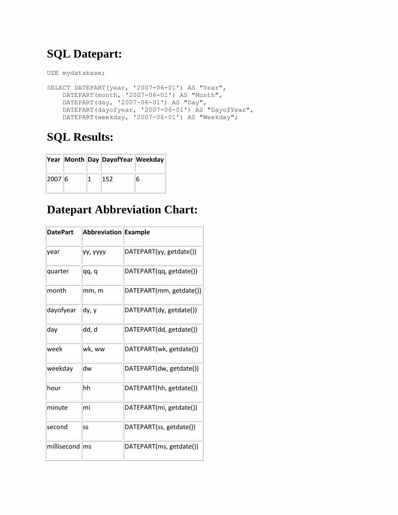
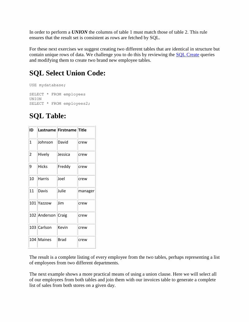
Page 1
A Short Oracle Tutorial For Beginners
This is just a short introduction to Oracle for beginners, to give a brief history of databases and
Oracle's role in that history, explain relational theory and provide a few practical examples to
show how relational databases work. If you would like to learn more just contact us and ask for
our free tutorial.
History of Databases - From Trees To Objects
The storage and management of data is probably the biggest headache for all businesses.
It has been so for a long while and is likely to continue for a long while too. As companies aim to
store more and more details about their customers and their buying habits, they need to store and
manage more and more data. The only way this can be done efficiently and at a reasonable cost
is by the use of computers.
In the late 1960s/early 1970s, specialised data management software appeared - the first database
management systems (DBMS). These early DBMS were either
hierarchical (tree) or network (CODASYL) databases and were, thererfore, very complex and
inflexible which made life difficult when it came to adding new applications or reorganising the
data.
The solution to this was relational databases which are based on the concept of normalisation -
the separation of the logical and physical representation of data.
In 1970 the relational data model was defined by E.F. Codd (see "A Relational Model of Data for
Large Shared Data Banks" Comm. ACM. 13 (June 6, 1970), 377-387).
Page 2
In 1974 IBM started a project called System/R to prove the theory of relational databases. This
led to the development of a query language called SEQUEL (Structured English Query
Language) later renamed to Structured Query Language (SQL) for legal reasons and now the
query language of all databases.
In 1978 a prototype System/R implementation was evaluated at a number of IBM customer sites.
By 1979 the project finished with the conclusion that relational databases were a feasible
commercial product.
Meanwhile, IBM's research into relational databases had come to the attention of a group of
engineers in California. They were so convinced of the potential that they formed a company
called Relational Software, Inc. in 1977 to build such a database. Their product was called
Oracle and the first version for VAX/VMS was released in 1979, thereby becoming the first
commercial rdbms, beating IBM to market by 2 years.
In the 1980s the company was renamed to Oracle Corporation. Throughout the 1980s, new
features were added and performance improved as the price of hardware came down and Oracle
became the largest independent rdbms vendor. By 1985 they boasted of having more than 1000
installations.
As relational databases became accepted, companies wanted to expand their use to store images,
spreadsheets, etc. which can't be described in 2-dimensional terms. This led to the Oracle
database becoming an object-relational hybrid in version 8.0, i.e. a relational database with
object extensions, enabling you to have the best of both worlds.
Click on the link to continue this Oracle tutorial .
For Better, Faster, Smarter, Oracle Training and Consultancy
A Short Oracle Tutorial For Beginners (ctd)
What is a relational database?
As mentioned before, a relational database is based on the separation and independence of the
the logical and physical representations of the data. This provides enormous flexibility and
Page 3
means you can store the data physically in any way without affecting how the data is presented
to the end user. The separation
of physical and logical layers means that you can change either layer without affecting the other.
A relational database can be regarded as a set of 2-dimensional tables which are known as
"relations" in relational database theory. Each table has rows ("tuples") and columns
("domains"). The relationships between the tables is defined by one table having a column with
the same meaning (but not necessarily value) as a column in another table.
For example consider a database with just 2 tables :
emp(id number
,name varchar2(30)
,job_title varchar2(20)
,dept_id number)
holding employee information and
dept(id number
,name varchar2(30))
holding department information.
There is an implied relationship between these tables because emp has a column called dept_id
which is the same as the id column in dept. In Oracle this is usually implemented by what's
called a foreign-key relationship which prevents values being stored that are not present in the
referenced table.
Relational databases obtain their flexibility from being based on set theory (also known as
relational calculus) which enables sets or relations to be combined in various ways, including:
join/intersection union (i.e. the sum of 2 sets); exclusive "OR" (i.e. the difference between 2 sets) and outer-join which is a combination of intersecting and exclusive or ing.
Page 4
The intersection or join between 2 sets (in this case, tables) produces only those elements that
exist in both sets.
Therefore, if we join Emp and Dept on department id, we will be left with only those employees
who work for a department that is in the dept table and only those departments which have
employees who are in the emp table.
The union produces the sum of the tables - meaning all records in Emp and all records in Dept.
and this may be with or without duplicates.
Let's use the following data to provide specific examples:
Emp
Id Name Dept Id
1 Bill Smith 3
2 Mike Lewis 2
3 Ray Charles 3
4 Andy Mallory 4
5 Mandy Randall 6
6 Allison White 1
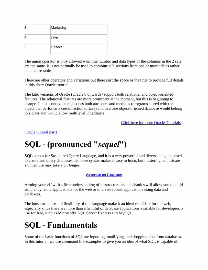
Dept
Id Name
1 HR
2 IT
3 Marketing
4 Sales
5 Finance
Page 5
The join of Emp and Dept. on the department id would produce the following result:
Emp.Id Emp.Name Dept.Id Dept.Name
1 Bill Smith 3 Marketing
2 Mike Lewis 2 IT
3 Ray Charles 3 Marketing
4 Andy Mallory 4 Sales
6 Allison White 1 HR
The union of Emp and Dept. would produce the following results
Id Name
1 Bill Smith
2 Mike Lewis
3 Ray Charles
4 Andy Mallory
5 Mandy Randall
1 HR
2 IT
Page 6
3 Marketing
4 Sales
5 Finance
The union operator is only allowed when the number and data types of the columns in the 2 sets
are the same. It is not normally be used to combine sub sections from one or more tables rather
than entire tables.
There are other operators and variations but there isn't the space or the time to provide full details
in this short Oracle tutorial.
The later versions of Oracle (Oracle 8 onwards) support both relational and object-oriented
features. The relational features are more prominent at the moment, but this is beginning to
change. In this context an object has both attributes and methods (programs stored with the
object that performs a certain action or task) and in a true object-oriented database would belong
to a class and would allow multilevel inheritance.
Click here for more Oracle Tutorials
Oracle tutorial part1
SQL - (pronounced "sequel")
SQL stands for Structured Query Language, and it is a very powerful and diverse language used
to create and query databases. Its loose syntax makes it easy to learn, but mastering its intricate
architecture may take a bit longer.
Advertise on Tizag.com
Arming yourself with a firm understanding of its structure and mechanics will allow you to build
simple, dynamic applications for the web or to create robust applications using data and
databases.
The loose structure and flexibility of this language make it an ideal candidate for the web,
especially since there are more than a handful of database applications available for developers o
use for free, such as Microsoft's SQL Server Express and MySQL.
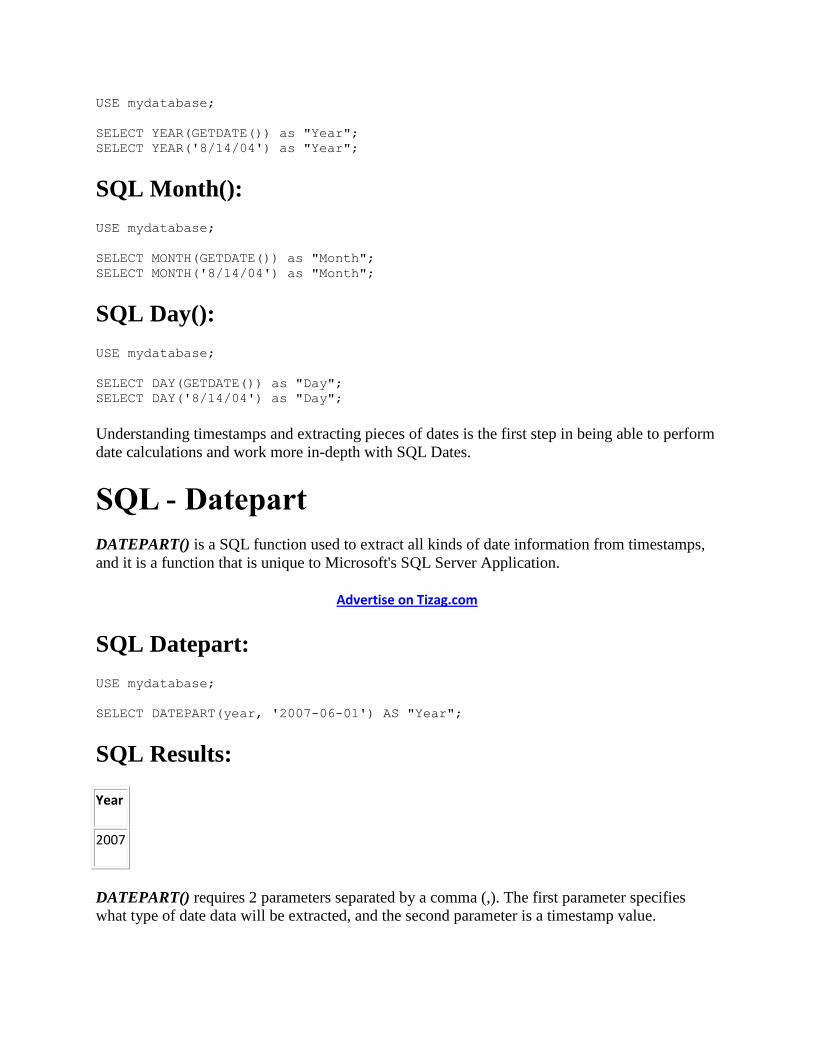
SQL - Fundamentals
Some of the basic functions of SQL are inputting, modifying, and dropping data from databases.
In this tutorial, we use command line examples to give you an idea of what SQL is capable of.
Page 7
Coupled with the use of web languages such as HTML and PHP, SQL becomes an even greater
tool for building dynamic web applications.
SQL - Tutorial Scope
Reading further, you will encounter a number of hands-on examples intended to introduce you to
SQL. The majority of these examples are intended to span across the different available
variations of SQL, but the primary focus of this tutorial is Microsoft's SQL Server Express.
SQL - Getting Started
To get started, you will need to install Microsoft SQL Server Express. For installation help, we
suggest you go straight to the developer homepage:
SQL Server Express Download:
SQL Server
It is preferred that you select SQL Server Express 2008 for this tutorial. This version of SQL is
available for private use for free, and we've provided the link to Microsoft's site, or you can find
the download page by searching for "SQL Server Express" on Google.
Follow the online installation guide that Microsoft provides, and launch SQL Server
Management Studio Express to connect to your SQL database. This Management Studio
Application will be your temporary home for the remainder of the tutorial.
SQL - World Wide Web
Building a website on SQL architecture is quickly becoming the standard among web 2.0 sites.
With a SQL backend, it is fairly simple to store user data, email lists, or other kinds of dynamic
data. E-Commerce web sites, community sites, and online web services rely on SQL databases to
manage user data or process user purchases.
SQL has become popular among web developers due to its flexibility and simplicity. With some
basic knowledge of HTML, PHP, and a database program such as Microsoft's SQL Server, a
developer becomes capable of creating complex websites and applications while relying on
online web services to provide a SQL backend in which user data is stored. This tutorial will
provide you with just a small taste of this type of programming and architecture.
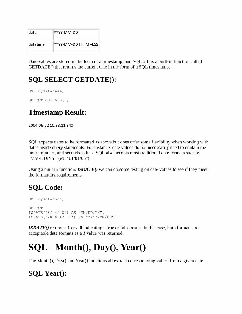
SQL - Databases
Page 8
What's a Database? A SQL database is nothing more than an empty shell, like a vacant
warehouse. It offers no real functionality whatsoever, but does provide a virtual space to store
data. Data is stored inside of database objects called tables, and tables are the containers that
actually hold specific types of data, such as numbers, files, strings, and dates.
Advertise on Tizag.com
A single database can house hundreds of tables containing more than 1,000 table columns each
and they may be jam packed with relational data ready to be retrieved by SQL. Perhaps the
greatest feature SQL offers is that it doesn't take much effort to rearrange your warehouse to
meet your ever-growing business needs.
SQL - Creating a Database
Creating a database inside of SQL Express has its advantages. After launching Microsoft's SQL
Server Management Studio Express application, simply right-clicking on the Databases folder of
the Object Explorer gives you the option to create a New Database. After selecting the New
Database... option, name your database "MyDatabase" and press "OK".
Now is the time to press the New Query button located toward the top of the screen, just above
the Object Explorer pane.
Pressing this button offers an empty tab. All SQL query statements (code) that we will be
exploring will be entered here and executed against the SQL Express database.
If you haven't yet created a new database, you may also create a database by typing the following
SQL query statement into your new empty query tab, and then pressing the Execute button or
striking the (F5) key.
SQL Create Database Query:
CREATE DATABASE MyDatabase;
After executing this query, SQL will notify you that your query has run successfully and that the
database was created successfully. If you receive an error message instead, Google the error
Page 9
message for troubleshooting advice. (Vista users must verify that they are running SQL Server
Management Studio Express with administrator privileges.)
Congratulations! You have executed your first SQL command and written what is perhaps your
first bit of SQL code.
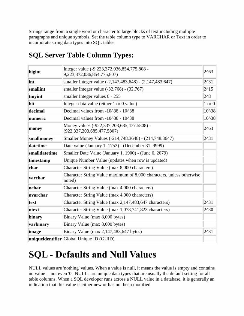
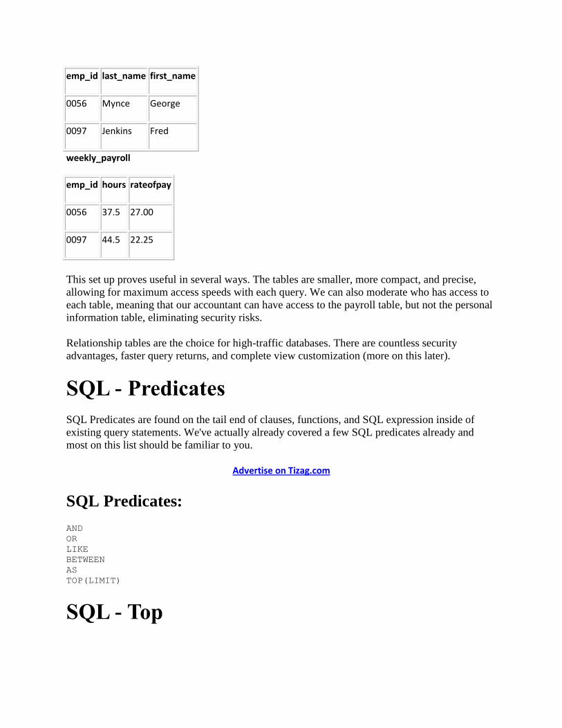
SQL - Tables
Data is stored inside SQL tables which are contained within SQL databases. A single database
can house hundreds of tables, each playing its own unique role in the database schema. While
database architecture and schema are concepts far above the scope of this tutorial, we plan on
diving in just past the surface to give you a glimpse of database architecture that begins with a
thorough understanding of SQL Tables.
Advertise on Tizag.com
SQL tables are comprised of table rows and columns. Table columns are responsible for storing
many different types of data, like numbers, texts, dates, and even files. There are many different
types of table columns and these data types vary, depending on how the SQL table has been
created by the SQL developer. A table row is a horizontal record of values that fit into each
different table column.
SQL - Create a SQL Table
Let's now CREATE a SQL table to help us expand our knowledge of SQL and SQL commands.
This new table will serve as a practice table and we will begin to populate this table with some
data which we can then manipulate as more SQL Query commands are introduced. The next
couple of examples will definitely be overwhelming to novice SQL programmers, but we will
take a moment to explain what's going on.
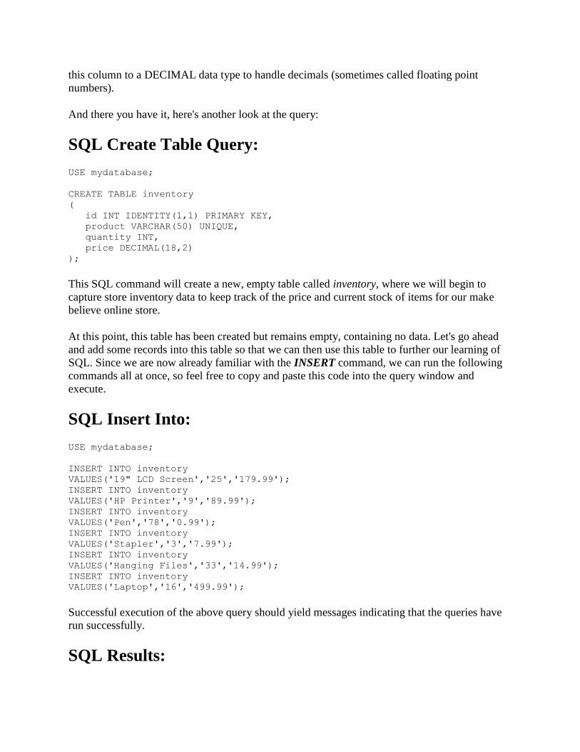
SQL Create Table Query:
USE mydatabase;
CREATE TABLE orders
(id INT IDENTITY(1,1) PRIMARY KEY,
customer VARCHAR(50),
day_of_order DATETIME,
product VARCHAR(50),
quantity INT);
The first line of the example, "USE mydatabase;", is pretty straightforward. This line defines the
query scope and directs SQL to run the command against the MyDatabase object we created
earlier in the SQL Databases lesson. The blank line break after the first command is not required,
Page 10
but it makes our query easier to follow. The line starting with the CREATE clause is where we
are actually going to tell SQL to create the new table, which is named orders.
Each table column has its own set of guidelines or schema, and the lines of code above contained
in parenthesis () are telling SQL how to go about setting up each column schema. Table columns
are presented in list format, and each schema is separated with a comma (,). It isn't important to
fully understand exactly what all of these schema details mean just yet. They will be explained in
more detail throughout the remainder of the tutorial. For now, just take note that we are creating
a new, empty SQL table named orders, and this table is 5 columns wide.
SQL - INSERT DATA into your New Table
Next, we will use SQL's INSERT command to draw up a query that will insert a new data row
into our brand new SQL table, orders. If you're already familiar with everything we've covered
so far, please execute the query below and then skip ahead and start learning about other SQL
Queries.
SQL Insert Query:
USE mydatabase;
INSERT INTO orders
(customer,day_of_order,product, quantity)
VALUES('Tizag','8/1/08','Pen',4);
SQL Insert Query Results:
(1 row(s) affected)
This message ("1 row(s) affected") indicates that our query has run successfully and also informs
us that 1 row has been affected by the query. This is the desired result as our goal was to insert a
single record into the newly formed orders table.
Listed above is a typical INSERT query used to insert data into the table we had previously
created. The first line ("USE mydatabase;") identifies the query scope and the line after indicates
what it is we'd like SQL to do for us. ("INSERT INTO orders") inserts data into the orders table.
Then, we have to list each table column by name (customer,day_of_order,product, quantity) and
finally provide a list of values to insert into each table column VALUES('Tizag','8/1/08','Pen',4).
You may notice that we have not included the id column, and this is intentional. We have set this
column up in a way that allows SQL to populate this field automatically, and therefore, we do
not need to worry about including it in any of our INSERT statements. (More on this later.)
Page 11
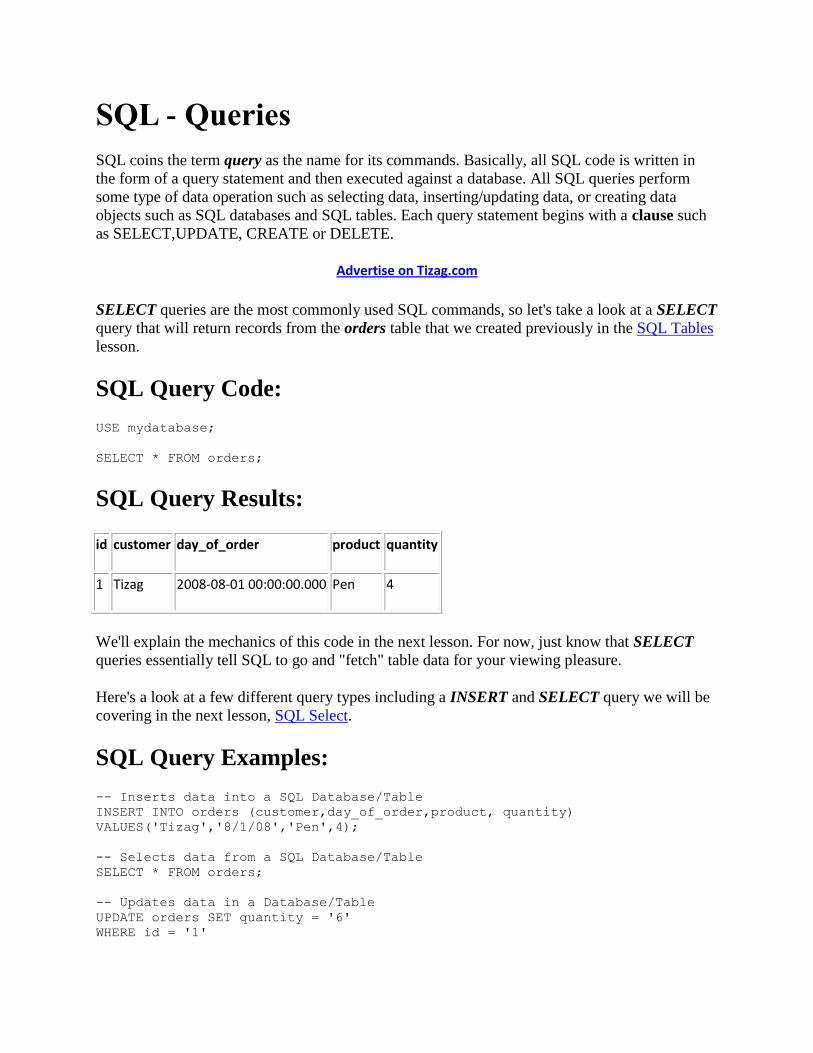
SQL - Queries
SQL coins the term query as the name for its commands. Basically, all SQL code is written in
the form of a query statement and then executed against a database. All SQL queries perform
some type of data operation such as selecting data, inserting/updating data, or creating data
objects such as SQL databases and SQL tables. Each query statement begins with a clause such
as SELECT,UPDATE, CREATE or DELETE.
Advertise on Tizag.com
SELECT queries are the most commonly used SQL commands, so let's take a look at a SELECT
query that will return records from the orders table that we created previously in the SQL Tables
lesson.
SQL Query Code:
USE mydatabase;
SELECT * FROM orders;
SQL Query Results:
id customer day_of_order product quantity
1 Tizag 2008-08-01 00:00:00.000 Pen 4
We'll explain the mechanics of this code in the next lesson. For now, just know that SELECT
queries essentially tell SQL to go and "fetch" table data for your viewing pleasure.
Here's a look at a few different query types including a INSERT and SELECT query we will be
covering in the next lesson, SQL Select.
SQL Query Examples:
-- Inserts data into a SQL Database/Table
INSERT INTO orders (customer,day_of_order,product, quantity)
VALUES('Tizag','8/1/08','Pen',4);
-- Selects data from a SQL Database/Table
SELECT * FROM orders;
-- Updates data in a Database/Table
UPDATE orders SET quantity = '6'
WHERE id = '1'
Page 12
More information about these queries can be found at the following links: SQL Insert, SQL
Update, SQL Delete
SQL - Query Structure Review
Structurally, each SQL query we have seen in this lesson are similar. Each start with a clause
telling SQL which operation to perform and the remaining lines provide more detailed
information as to how we want SQL to go about performing each SQL Command.
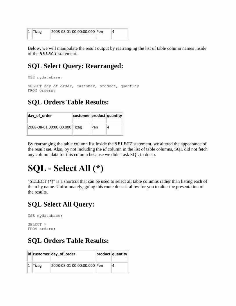
SQL - Select
SQL SELECT may be the most commonly used command by SQL programmers. It is used to
extract data from databases and to present data in a user-friendly table called the result set.
Advertise on Tizag.com
SQL Select Query Template:
SELECT table_column1, table_column2, table_column3
FROM my_table;
Select queries require two essential parts. The first part is the "WHAT", which determines what
we want SQL to go and fetch. The second part of any SELECT command is the "FROM
WHERE". It identifies where to fetch the data from, which may be from a SQL table, a SQL
view, or some other SQL data object.
Now we would like SQL to go and fetch some data for us from the orders table that was created
in the previous lesson. How do we translate this request into SQL code so that the database
application does all the work for us? Simple! We just need to tell SQL what we want to select
and from where to select the data, by following the schema outlined below.
SQL Select Query Code:
USE mydatabase;
SELECT id, customer, day_of_order, product, quantity
FROM orders;
SQL Orders Table Results:
id customer day_of_order product quantity
Page 13
1 Tizag 2008-08-01 00:00:00.000 Pen 4
Below, we will manipulate the result output by rearranging the list of table column names inside
of the SELECT statement.
SQL Select Query: Rearranged:
USE mydatabase;
SELECT day_of_order, customer, product, quantity
FROM orders;
SQL Orders Table Results:
day_of_order customer product quantity
2008-08-01 00:00:00.000 Tizag Pen 4
By rearranging the table column list inside the SELECT statement, we altered the appearance of
the result set. Also, by not including the id column in the list of table columns, SQL did not fetch
any column data for this column because we didn't ask SQL to do so.
SQL - Select All (*)
"SELECT (*)" is a shortcut that can be used to select all table columns rather than listing each of
them by name. Unfortunately, going this route doesn't allow for you to alter the presentation of
the results.
SQL Select All Query:
USE mydatabase;
SELECT *
FROM orders;
SQL Orders Table Results:
id customer day_of_order product quantity
1 Tizag 2008-08-01 00:00:00.000 Pen 4
Page 14
SQL - Selecting Data
The (*) query statement should be used with caution. Using this against our little tutorial
database will surely do no harm, but using this query against an extremely large database may
not be the best practice. Large databases may have web services or applications attached to them,
so frequently updating and accessing large quantities data may temporarily lock a table for
fractions of a second or more. If this disruption happens to occur just as some piece of data is
being updated, you may experience data corruption.
Taking every precaution to avoid data corruption is in your best interest as a new SQL
programmer. Corrupted data may be lost and never recovered, and it can lead to even more
corruption inside a database. The best habits are to be as precise as possible, and in the case of
select statements, this often means selecting minimal amounts of data when possible.
At this point, you should feel comfortable with SELECT and how to look into your database and
see actual data rows residing inside of tables. This knowledge will prove invaluable as your SQL
skills develop beyond the basics and as you begin to tackle larger, more advanced SQL projects.
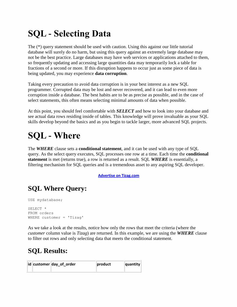
SQL - Where
The WHERE clause sets a conditional statement, and it can be used with any type of SQL
query. As the select query executes, SQL processes one row at a time. Each time the conditional
statement is met (returns true), a row is returned as a result. SQL WHERE is essentially, a
filtering mechanism for SQL queries and is a tremendous asset to any aspiring SQL developer.
Advertise on Tizag.com
SQL Where Query:
USE mydatabase;
SELECT *
FROM orders
WHERE customer = 'Tizag'
As we take a look at the results, notice how only the rows that meet the criteria (where the
customer column value is Tizag) are returned. In this example, we are using the WHERE clause
to filter out rows and only selecting data that meets the conditional statement.
SQL Results:
id customer day_of_order product quantity
Page 15
1 Tizag 2008-08-01 00:00:00.000 Pen 4
2 Tizag 2008-08-01 00:00:00.000 Stapler 1
5 Tizag 2008-07-25 00:00:00.000 19" LCD Screen 3
6 Tizag 2008-07-25 00:00:00.000 HP Printer 2
Conditional statements are not unique to SQL, and neither are operators. Operators are symbols
such as (=) or (<), and they are seen inside of conditional statements and expressions in SQL and
other programming languages. While we're not going to dive into much detail about the different
kinds of operators yet, it is a good idea to be familiar with them and be able to recognize them
inside of conditional statements as we look over the next few examples.
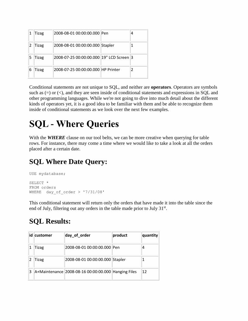
SQL - Where Queries
With the WHERE clause on our tool belts, we can be more creative when querying for table
rows. For instance, there may come a time where we would like to take a look at all the orders
placed after a certain date.
SQL Where Date Query:
USE mydatabase;
SELECT *
FROM orders
WHERE day_of_order > '7/31/08'
This conditional statement will return only the orders that have made it into the table since the
end of July, filtering out any orders in the table made prior to July 31st.
SQL Results:
id customer day_of_order product quantity
1 Tizag 2008-08-01 00:00:00.000 Pen 4
2 Tizag 2008-08-01 00:00:00.000 Stapler 1
3 A+Maintenance 2008-08-16 00:00:00.000 Hanging Files 12
Page 16
4 Gerald Garner 2008-08-15 00:00:00.000 19" LCD Screen 3
Notice how the date value is formatted inside the conditional statement. We passed a value
formatted MM/DD/YY, and we've completely neglected the hours, minutes, and seconds values,
yet SQL is intelligent enough to understand this. Therefore, our query is successfully executed.
SQL - Where with Multiple Conditionals
A WHERE statement can accept multiple conditional statements. What this means is that we are
able to select rows meeting two different conditions at the same time.
Perhaps the easiest way to go about this is to add another condition to the previous example,
where we retrieved only the orders placed after July 31st. We can take this example one step
further and link two conditional statements together with "AND".
SQL Where And:
USE mydatabase;
SELECT *
FROM orders
WHERE day_of_order > '7/31/08'
AND customer = 'Tizag'
At this point, we have sent SQL two conditional statements with a single WHERE clause,
essentially applying two filters to the expected result set.
SQL Results:
id customer day_of_order product quantity
1 Tizag 2008-08-01 00:00:00.000 Pen 4
2 Tizag 2008-08-01 00:00:00.000 Stapler 1
By applying the AND clause, SQL has now been asked to return only rows that meet both
conditional statements. In this case, we would like to return all orders that were made before July
31st and made by a specific company - which is, in this case, Tizag. We have more examples of
SQL AND/OR. Just follow the link.
SQL - As
Page 17
SQL AS temporarily assigns a table column a new name. This grants the SQL developer the
ability to make adjustments to the presentation of query results and allow the developer to label
results more accurately without permanently renaming table columns.
Advertise on Tizag.com
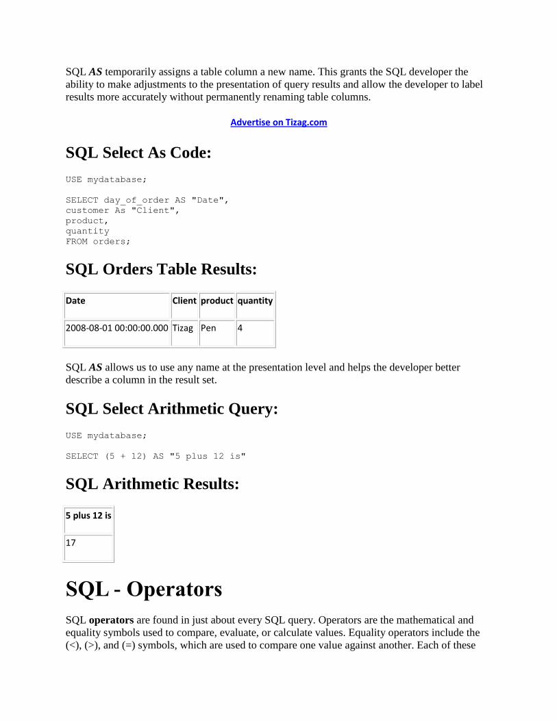
SQL Select As Code:
USE mydatabase;
SELECT day_of_order AS "Date",
customer As "Client",
product,
quantity
FROM orders;
SQL Orders Table Results:
Date Client product quantity
2008-08-01 00:00:00.000 Tizag Pen 4
SQL AS allows us to use any name at the presentation level and helps the developer better
describe a column in the result set.
SQL Select Arithmetic Query:
USE mydatabase;
SELECT (5 + 12) AS "5 plus 12 is"
SQL Arithmetic Results:
5 plus 12 is
17
SQL - Operators
SQL operators are found in just about every SQL query. Operators are the mathematical and
equality symbols used to compare, evaluate, or calculate values. Equality operators include the
(<), (>), and (=) symbols, which are used to compare one value against another. Each of these
Page 18
characters have special meaning, and when SQL comes across them, they help tell SQL how to
evaluate an expression or conditional statement. Most operators will appear inside of conditional
statements in the WHERE clause of SQL Commands.
Advertise on Tizag.com
Operators come in three flavors: mathematical, logical, and equality. Mathematical operators
add, subtract, multiply, and divide numbers. Logical operators include AND and OR. Take note
of the following tables for future reference.
SQL operators are generally found inside of queries-- more specifically, in the conditional
statements of the WHERE clause.
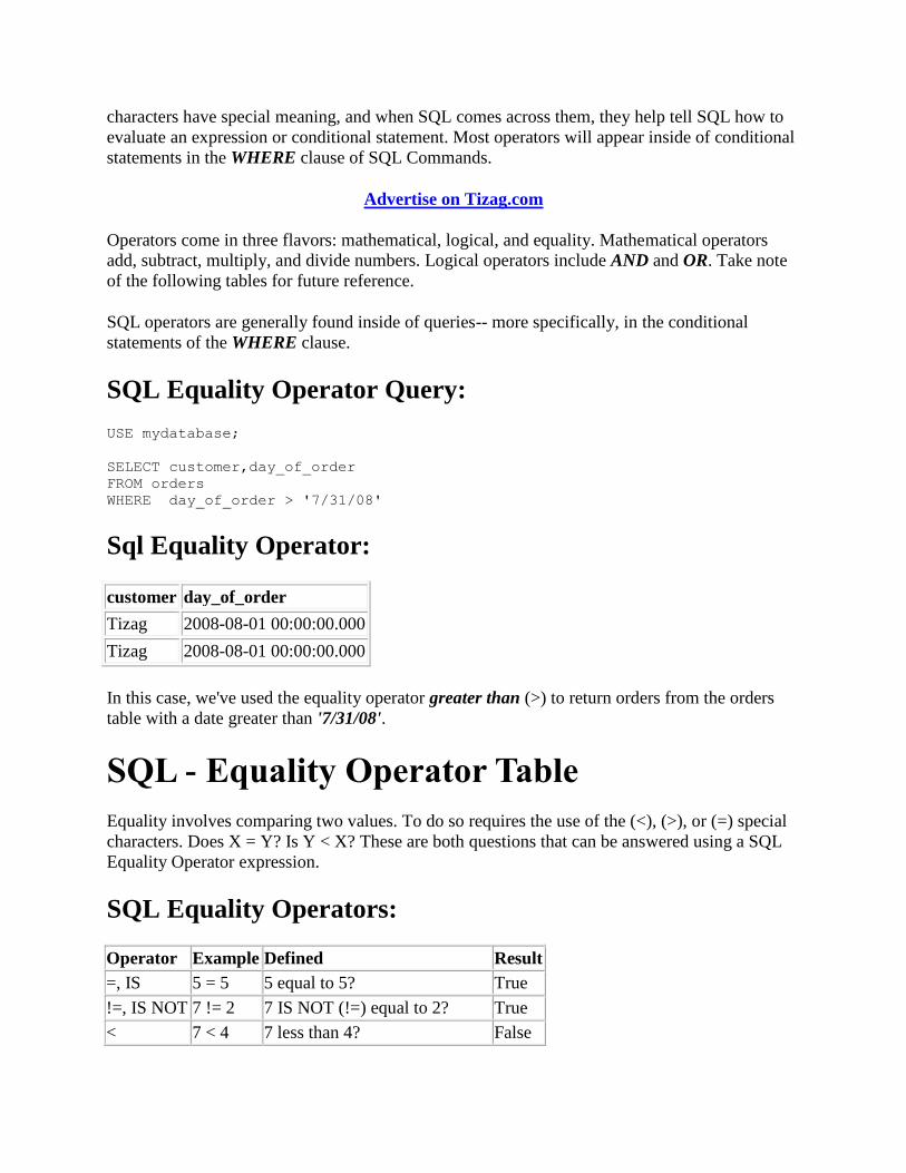
SQL Equality Operator Query:
USE mydatabase;
SELECT customer,day_of_order
FROM orders
WHERE day_of_order > '7/31/08'
Sql Equality Operator:
customer day_of_order
Tizag 2008-08-01 00:00:00.000
Tizag 2008-08-01 00:00:00.000
In this case, we've used the equality operator greater than (>) to return orders from the orders
table with a date greater than '7/31/08'.
SQL - Equality Operator Table
Equality involves comparing two values. To do so requires the use of the (<), (>), or (=) special
characters. Does X = Y? Is Y < X? These are both questions that can be answered using a SQL
Equality Operator expression.
SQL Equality Operators:
Operator Example Defined Result
=, IS 5 = 5 5 equal to 5? True
!=, IS NOT 7 != 2 7 IS NOT (!=) equal to 2? True
< 7 < 4 7 less than 4? False
Page 19
> 7 > 4 greater than 4? True
<= 7 <= 11 Is 7 less than or equal to 11? True
>= 7 >= 11 Is 7 greater than or equal to 11? False
SQL - Mathematical Operators
SQL mathematical operations are performed using mathematical operators (+, -, *, /, and %). We
can use SQL like a calculator to get a feel for how these operators work.
SQL Mathematical Operators:
SELECT
15 + 4, --Addition
15 - 4, --Subtraction
15 * 4, --Multiplication
15 / 5, -- Division
15 % 4; --Modulus
SQL Results:
Addition Subtraction Multiplication Division Modulus
19 11 60 3 3
Modulus may be the only unfamiliar term on the chart. Modulus performs division, dividing the
first digit by the second digit, but instead of returning a quotient, a "remainder" value is returned
instead.
Modulus Example:
USE mydatabase;
SELECT (5 / 2) -- = 2.5
SELECT (5 % 2) -- = 1 is the value that will be returned
SQL - Logical Operators
These operators provide you with a way to specify exactly what you want SQL to go and fetch,
and you may be as specific as you'd like! We'll discuss these a little later on and provide some
real world scenarios as well.
We cover these operators thoroughly in the SQL AND/OR lesson.
AND - Compares/Associates two values or expressions
Page 20
OR - Compares/Associates two values or expressions
QL - Create
SQL CREATE is the command used to create data objects, including everything from new
databases and tables to views and stored procedures. In this lesson, we will be taking a closer
look at how table creation is executed in the SQL world and offer some examples of the different
types of data a SQL table can hold, such as dates, number values, and texts.
Advertise on Tizag.com
To accomplish this, it is best to first take a look at the entire CREATE TABLE query and then
review each line individually.
SQL Create Table Code:
USE mydatabase;
CREATE TABLE inventory
(
id INT IDENTITY(1,1) PRIMARY KEY,
product VARCHAR(50) UNIQUE,
quantity INT,
price DECIMAL(18,2)
);
Line 1 identifies the scope of the query specifying a target database for query execution (USE
mydatabase) and we've seen it before so let's skip ahead to the next line, line 2 (CREATE
TABLE inventory). This line informs SQL of the plan to create a new table using the CREATE
clause and specifies the name of the new table (inventory). In this case, we plan on creating an
inventory table to maintain a current inventory of store items for an imaginary e-commerce web
site.
SQL Create Line 3:
id INT IDENTITY(1,1) PRIMARY KEY,
Line 3 should appear more foreign as there is a lot of information embedded in this line, but it is
not as hard as it seems. This is the first line that declares how to set up the first table column
inside the new inventory table.
id = The name of this new table column.
INT = The data type. INT is short for integer.
The first word, id, is the name of this new column and the second word declares the data type,
INT (integers). SQL will now expect this table column to house only integer data type values.
Page 21
IDENTITY (1,1) = The id column will be an identity column.
The next phrase, IDENTITY (1, 1) is a very special attribute and when a table column is marked
as an identity column, the column essentially turns into an automated counter. As new rows are
inserted into the table, this column value will automatically increment (count up). The
parameters (1,1) tell SQL which number to start counting from and by how many to increment
each value. In this case, we'll start with 1, and increment by 1 each time a new row is inserted
into our database. For example, the first INSERT command run against the inventory table will
have an id value of 1, and each consecutive row inserted thereafter will increment by one (1, 2, 3,
4 ... etc). This identity table column is essentially counting each inserted row and also ensuring
that we have a unique identifier value. This is important since this column has also been
identified as a primary key (see below).
PRIMARY KEY = This places a restraint on this column (no duplicate values)
Bringing up the tail-end of Line 3 is reserved for specifying any unique attributes to associate
with this table column. In this case, we have told SQL that this column will act as the PRIMARY
KEY for the inventory table. Declaring this column as the PRIMARY KEY places a restraint on
this column meaning no duplicate values may exist in this column and SQL will throw an error
message if an attempt is made to enter duplicate data. Since this row is set to automatically
increment each time a new record is added, we know that this column will always be a unique
value.
SQL Create Line 4:
product VARCHAR(50) UNIQUE,
Line 4 specifies the name and type of the second column in the inventory table. Product stands
for the inventory table product name and this column is set as a VARCHAR(50), which means it
will be able to handle numbers, letters, and special characters as values. In other words, "Any
words, numbers, or special characters can be placed into this column value, with a 50 character
limit."
The UNIQUE attribute tells SQL that this table column must be a UNIQUE value at all times.
This restraint will stop us from accidentally inserting duplicate records for the same product,
which will serve as an aid to us to help maintain data integrity.
SQL Create Line 5,6:
quantity INT,
price DECIMAL(18,2)
Now that you are more familiar with the structure of this query, lines 5 and 6 should look less
like a foreign language and more like SQL code. These lines are creating two more table
columns: quantity and price. Since the price column will be dealing with decimals, we have set
Page 22
this column to a DECIMAL data type to handle decimals (sometimes called floating point
numbers).
And there you have it, here's another look at the query:
SQL Create Table Query:
USE mydatabase;
CREATE TABLE inventory
(
id INT IDENTITY(1,1) PRIMARY KEY,
product VARCHAR(50) UNIQUE,
quantity INT,
price DECIMAL(18,2)
);
This SQL command will create a new, empty table called inventory, where we will begin to
capture store inventory data to keep track of the price and current stock of items for our make
believe online store.
At this point, this table has been created but remains empty, containing no data. Let's go ahead
and add some records into this table so that we can then use this table to further our learning of
SQL. Since we are now already familiar with the INSERT command, we can run the following
commands all at once, so feel free to copy and paste this code into the query window and
execute.
SQL Insert Into:
USE mydatabase;
INSERT INTO inventory
VALUES('19" LCD Screen','25','179.99');
INSERT INTO inventory
VALUES('HP Printer','9','89.99');
INSERT INTO inventory
VALUES('Pen','78','0.99');
INSERT INTO inventory
VALUES('Stapler','3','7.99');
INSERT INTO inventory
VALUES('Hanging Files','33','14.99');
INSERT INTO inventory
VALUES('Laptop','16','499.99');
Successful execution of the above query should yield messages indicating that the queries have
run successfully.
SQL Results:
Page 23
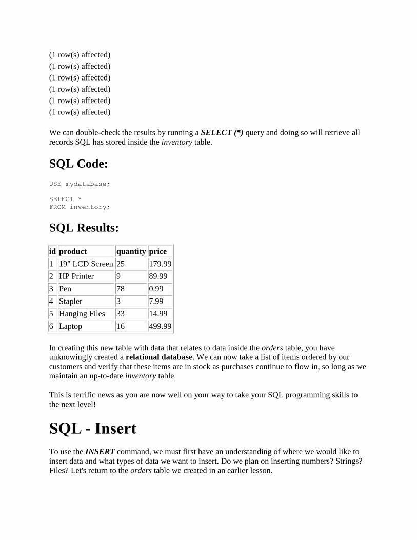
(1 row(s) affected)
(1 row(s) affected)
(1 row(s) affected)
(1 row(s) affected)
(1 row(s) affected)
(1 row(s) affected)
We can double-check the results by running a SELECT (*) query and doing so will retrieve all
records SQL has stored inside the inventory table.
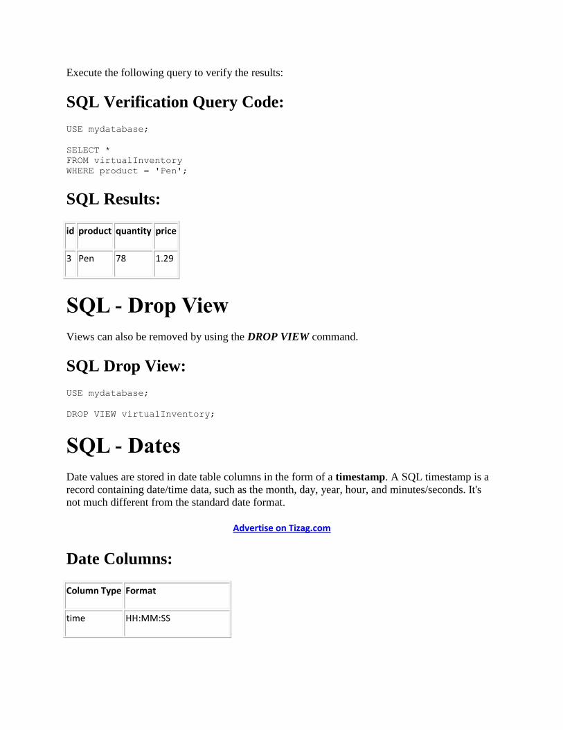
SQL Code:
USE mydatabase;
SELECT *
FROM inventory;
SQL Results:
id product quantity price
1 19" LCD Screen 25 179.99
2 HP Printer 9 89.99
3 Pen 78 0.99
4 Stapler 3 7.99
5 Hanging Files 33 14.99
6 Laptop 16 499.99
In creating this new table with data that relates to data inside the orders table, you have
unknowingly created a relational database. We can now take a list of items ordered by our
customers and verify that these items are in stock as purchases continue to flow in, so long as we
maintain an up-to-date inventory table.
This is terrific news as you are now well on your way to take your SQL programming skills to
the next level!
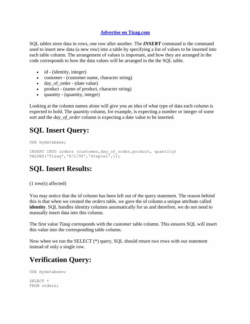
SQL - Insert
To use the INSERT command, we must first have an understanding of where we would like to
insert data and what types of data we want to insert. Do we plan on inserting numbers? Strings?
Files? Let's return to the orders table we created in an earlier lesson.
Page 24
Advertise on Tizag.com
SQL tables store data in rows, one row after another. The INSERT command is the command
used to insert new data (a new row) into a table by specifying a list of values to be inserted into
each table column. The arrangement of values is important, and how they are arranged in the
code corresponds to how the data values will be arranged in the the SQL table.
id - (identity, integer)
customer - (customer name, character string)
day_of_order - (date value)
product - (name of product, character string)
quantity - (quantity, integer)
Looking at the column names alone will give you an idea of what type of data each column is
expected to hold. The quantity column, for example, is expecting a number or integer of some
sort and the day_of_order column is expecting a date value to be inserted.
SQL Insert Query:
USE mydatabase;
INSERT INTO orders (customer,day_of_order,product, quantity)
VALUES('Tizag','8/1/08','Stapler',1);
SQL Insert Results:
(1 row(s) affected)
You may notice that the id column has been left out of the query statement. The reason behind
this is that when we created the orders table, we gave the id column a unique attribute called
identity. SQL handles identity columns automatically for us and therefore, we do not need to
manually insert data into this column.
The first value Tizag corresponds with the customer table column. This ensures SQL will insert
this value into the corresponding table column.
Now when we run the SELECT (*) query, SQL should return two rows with our statement
instead of only a single row.
Verification Query:
USE mydatabase;
SELECT *
FROM orders;
Page 25
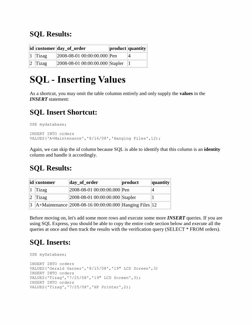
SQL Results:
id customer day_of_order product quantity
1 Tizag 2008-08-01 00:00:00.000 Pen 4
2 Tizag 2008-08-01 00:00:00.000 Stapler 1
SQL - Inserting Values
As a shortcut, you may omit the table columns entirely and only supply the values in the
INSERT statement:
SQL Insert Shortcut:
USE mydatabase;
INSERT INTO orders
VALUES('A+Maintenance','8/16/08','Hanging Files',12);
Again, we can skip the id column because SQL is able to identify that this column is an identity
column and handle it accordingly.
SQL Results:
id customer day_of_order product quantity
1 Tizag 2008-08-01 00:00:00.000 Pen 4
2 Tizag 2008-08-01 00:00:00.000 Stapler 1
3 A+Maintenance 2008-08-16 00:00:00.000 Hanging Files 12
Before moving on, let's add some more rows and execute some more INSERT queries. If you are
using SQL Express, you should be able to copy the entire code section below and execute all the
queries at once and then track the results with the verification query (SELECT * FROM orders).
SQL Inserts:
USE myDatabase;
INSERT INTO orders
VALUES('Gerald Garner','8/15/08','19" LCD Screen',3)
INSERT INTO orders
VALUES('Tizag','7/25/08','19" LCD Screen',3);
INSERT INTO orders
VALUES('Tizag','7/25/08','HP Printer',2);
Page 26
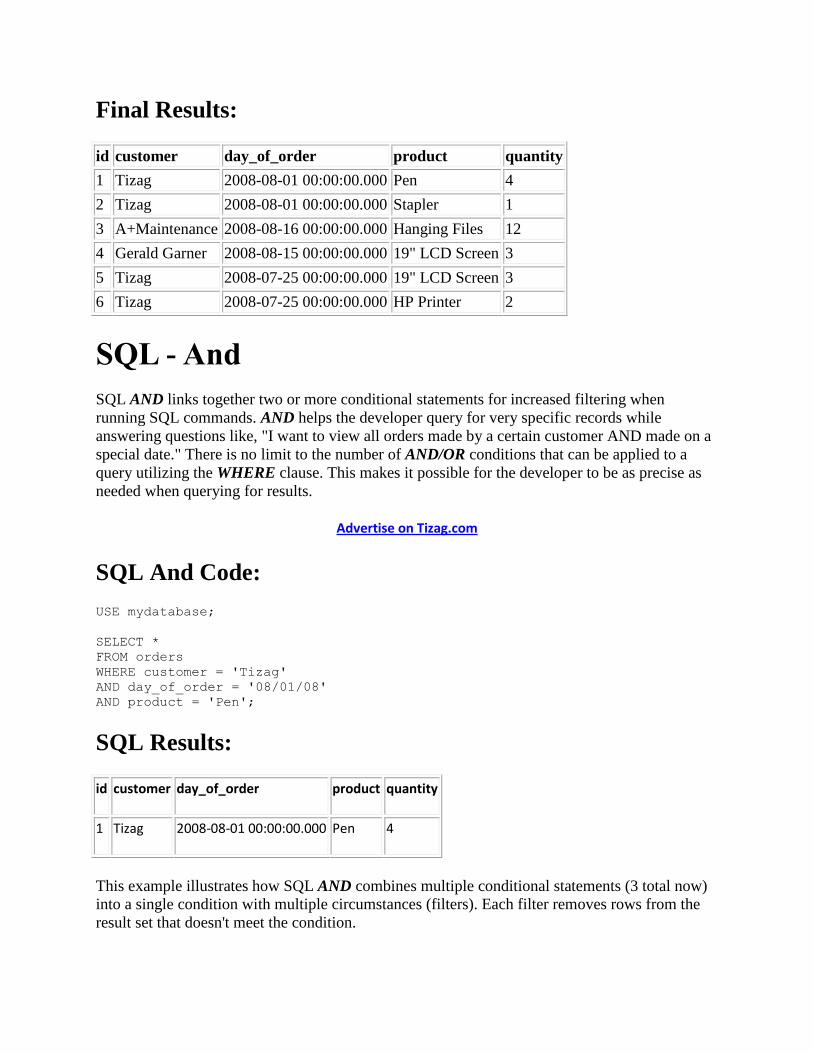
Final Results:
id customer day_of_order product quantity
1 Tizag 2008-08-01 00:00:00.000 Pen 4
2 Tizag 2008-08-01 00:00:00.000 Stapler 1
3 A+Maintenance 2008-08-16 00:00:00.000 Hanging Files 12
4 Gerald Garner 2008-08-15 00:00:00.000 19" LCD Screen 3
5 Tizag 2008-07-25 00:00:00.000 19" LCD Screen 3
6 Tizag 2008-07-25 00:00:00.000 HP Printer 2
SQL - And
SQL AND links together two or more conditional statements for increased filtering when
running SQL commands. AND helps the developer query for very specific records while
answering questions like, "I want to view all orders made by a certain customer AND made on a
special date." There is no limit to the number of AND/OR conditions that can be applied to a
query utilizing the WHERE clause. This makes it possible for the developer to be as precise as
needed when querying for results.
Advertise on Tizag.com
SQL And Code:
USE mydatabase;
SELECT *
FROM orders
WHERE customer = 'Tizag'
AND day_of_order = '08/01/08'
AND product = 'Pen';
SQL Results:
id customer day_of_order product quantity
1 Tizag 2008-08-01 00:00:00.000 Pen 4
This example illustrates how SQL AND combines multiple conditional statements (3 total now)
into a single condition with multiple circumstances (filters). Each filter removes rows from the
result set that doesn't meet the condition.
Page 27
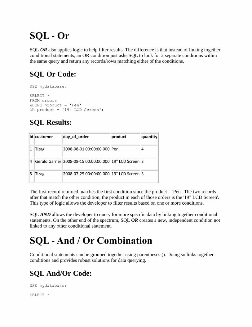
SQL - Or
SQL OR also applies logic to help filter results. The difference is that instead of linking together
conditional statements, an OR condition just asks SQL to look for 2 separate conditions within
the same query and return any records/rows matching either of the conditions.
SQL Or Code:
USE mydatabase;
SELECT *
FROM orders
WHERE product = 'Pen'
OR product = '19" LCD Screen';
SQL Results:
id customer day_of_order product quantity
1 Tizag 2008-08-01 00:00:00.000 Pen 4
4 Gerald Garner 2008-08-15 00:00:00.000 19" LCD Screen 3
5 Tizag 2008-07-25 00:00:00.000 19" LCD Screen 3
The first record returned matches the first condition since the product = 'Pen'. The two records
after that match the other condition; the product in each of those orders is the '19" LCD Screen'.
This type of logic allows the developer to filter results based on one or more conditions.
SQL AND allows the developer to query for more specific data by linking together conditional
statements. On the other end of the spectrum, SQL OR creates a new, independent condition not
linked to any other conditional statement.
SQL - And / Or Combination
Conditional statements can be grouped together using parentheses (). Doing so links together
conditions and provides robust solutions for data querying.
SQL And/Or Code:
USE mydatabase;
SELECT *
Page 28
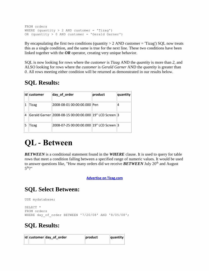
FROM orders
WHERE (quantity > 2 AND customer = 'Tizag')
OR (quantity > 0 AND customer = 'Gerald Garner')
By encapsulating the first two conditions (quantity > 2 AND customer = 'Tizag') SQL now treats
this as a single condition, and the same is true for the next line. These two conditions have been
linked together with the OR operator, creating very unique behavior.
SQL is now looking for rows where the customer is Tizag AND the quantity is more than 2, and
ALSO looking for rows where the customer is Gerald Garner AND the quantity is greater than
0. All rows meeting either condition will be returned as demonstrated in our results below.
SQL Results:
id customer day_of_order product quantity
1 Tizag 2008-08-01 00:00:00.000 Pen 4
4 Gerald Garner 2008-08-15 00:00:00.000 19" LCD Screen 3
5 Tizag 2008-07-25 00:00:00.000 19" LCD Screen 3
QL - Between
BETWEEN is a conditional statement found in the WHERE clause. It is used to query for table
rows that meet a condition falling between a specified range of numeric values. It would be used
to answer questions like, "How many orders did we receive BETWEEN July 20th and August
5th?"
Advertise on Tizag.com
SQL Select Between:
USE mydatabase;
SELECT *
FROM orders
WHERE day_of_order BETWEEN '7/20/08' AND '8/05/08';
SQL Results:
id customer day_of_order product quantity
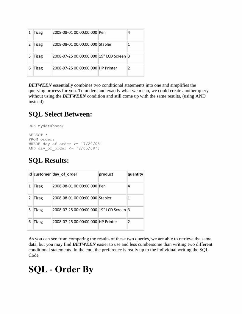
Page 29
1 Tizag 2008-08-01 00:00:00.000 Pen 4
2 Tizag 2008-08-01 00:00:00.000 Stapler 1
5 Tizag 2008-07-25 00:00:00.000 19" LCD Screen 3
6 Tizag 2008-07-25 00:00:00.000 HP Printer 2
BETWEEN essentially combines two conditional statements into one and simplifies the
querying process for you. To understand exactly what we mean, we could create another query
without using the BETWEEN condition and still come up with the same results, (using AND
instead).
SQL Select Between:
USE mydatabase;
SELECT *
FROM orders
WHERE day_of_order >= '7/20/08'
AND day_of_order <= '8/05/08';
SQL Results:
id customer day_of_order product quantity
1 Tizag 2008-08-01 00:00:00.000 Pen 4
2 Tizag 2008-08-01 00:00:00.000 Stapler 1
5 Tizag 2008-07-25 00:00:00.000 19" LCD Screen 3
6 Tizag 2008-07-25 00:00:00.000 HP Printer 2
As you can see from comparing the results of these two queries, we are able to retrieve the same
data, but you may find BETWEEN easier to use and less cumbersome than writing two different
conditional statements. In the end, the preference is really up to the individual writing the SQL
Code
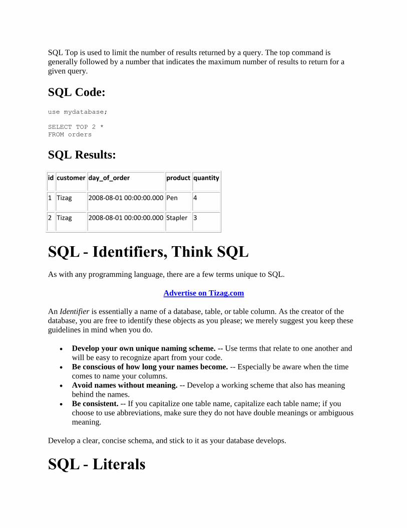
SQL - Order By
Page 30
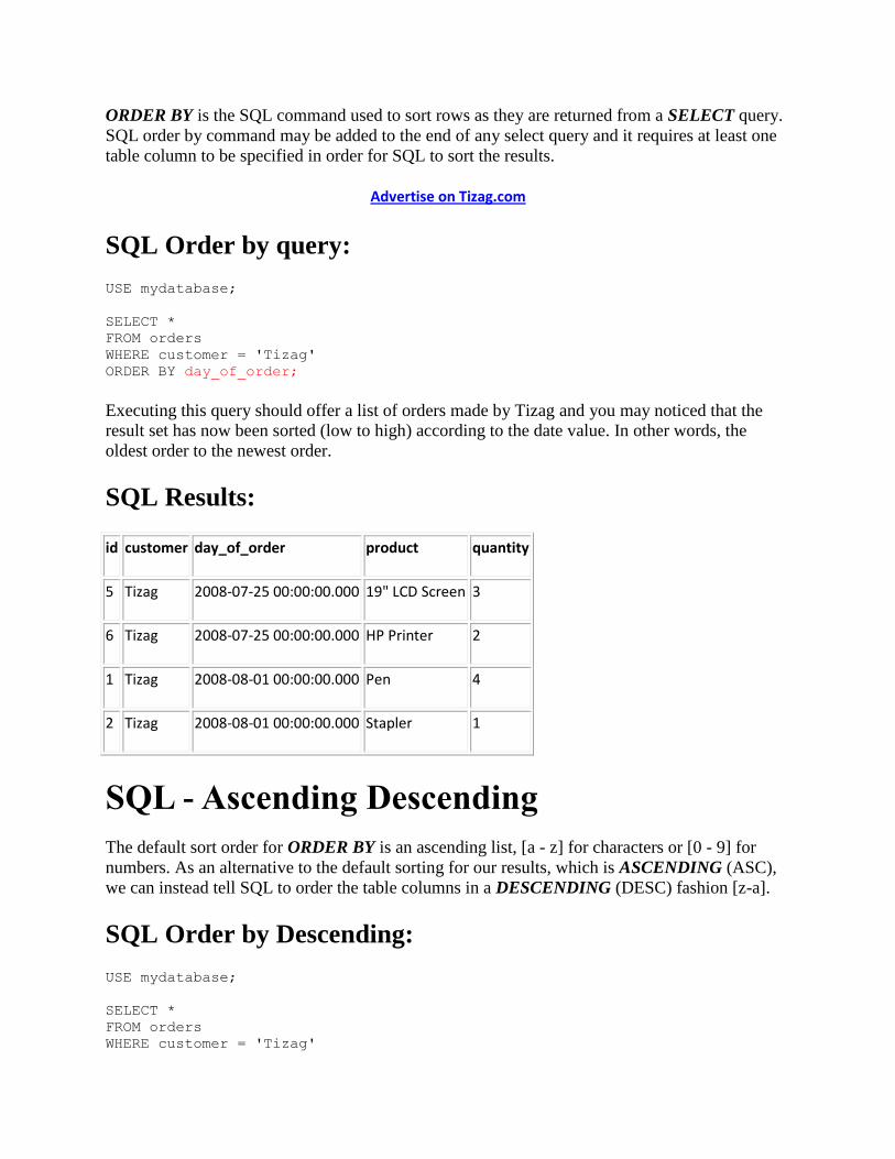
ORDER BY is the SQL command used to sort rows as they are returned from a SELECT query.
SQL order by command may be added to the end of any select query and it requires at least one
table column to be specified in order for SQL to sort the results.
Advertise on Tizag.com
SQL Order by query:
USE mydatabase;
SELECT *
FROM orders
WHERE customer = 'Tizag'
ORDER BY day_of_order;
Executing this query should offer a list of orders made by Tizag and you may noticed that the
result set has now been sorted (low to high) according to the date value. In other words, the
oldest order to the newest order.
SQL Results:
id customer day_of_order product quantity
5 Tizag 2008-07-25 00:00:00.000 19" LCD Screen 3
6 Tizag 2008-07-25 00:00:00.000 HP Printer 2
1 Tizag 2008-08-01 00:00:00.000 Pen 4
2 Tizag 2008-08-01 00:00:00.000 Stapler 1
SQL - Ascending Descending
The default sort order for ORDER BY is an ascending list, [a - z] for characters or [0 - 9] for
numbers. As an alternative to the default sorting for our results, which is ASCENDING (ASC),
we can instead tell SQL to order the table columns in a DESCENDING (DESC) fashion [z-a].
SQL Order by Descending:
USE mydatabase;
SELECT *
FROM orders
WHERE customer = 'Tizag'
Page 31
ORDER BY day_of_order DESC
SQL Results:
id customer day_of_order product quantity
1 Tizag 2008-08-01 00:00:00.000 Pen 4
2 Tizag 2008-08-01 00:00:00.000 Stapler 1
5 Tizag 2008-07-25 00:00:00.000 19" LCD Screen 3
6 Tizag 2008-07-25 00:00:00.000 HP Printer 2
If you compare these results to the results above, you should notice that we've pulled the same
information but it is now arranged in a reverse (descending) order.
SQL - Sorting on Multiple Columns
Results may be sorted on more than one column by listing multiple column names in the
ORDER BY clause, similar to how we would list column names in each SELECT statement.
SQL Order by Multiple columns:
USE mydatabase;
SELECT *
FROM orders
ORDER BY customer, day_of_order;
This query should alphabetize by customer, grouping together orders made by the same customer
and then by the purchase date. SQL sorts according to how the column names are listed in the
ORDER BY clause.
SQL Results:
id customer day_of_order product quantity
3 A+Maintenance 2008-08-16 00:00:00.000 Hanging Files 12
4 Gerald Garner 2008-08-15 00:00:00.000 19" LCD Screen 3
Page 32
5 Tizag 2008-07-25 00:00:00.000 19" LCD Screen 3
6 Tizag 2008-07-25 00:00:00.000 HP Printer 2
1 Tizag 2008-08-01 00:00:00.000 Pen 4
2 Tizag 2008-08-01 00:00:00.000 Stapler 1
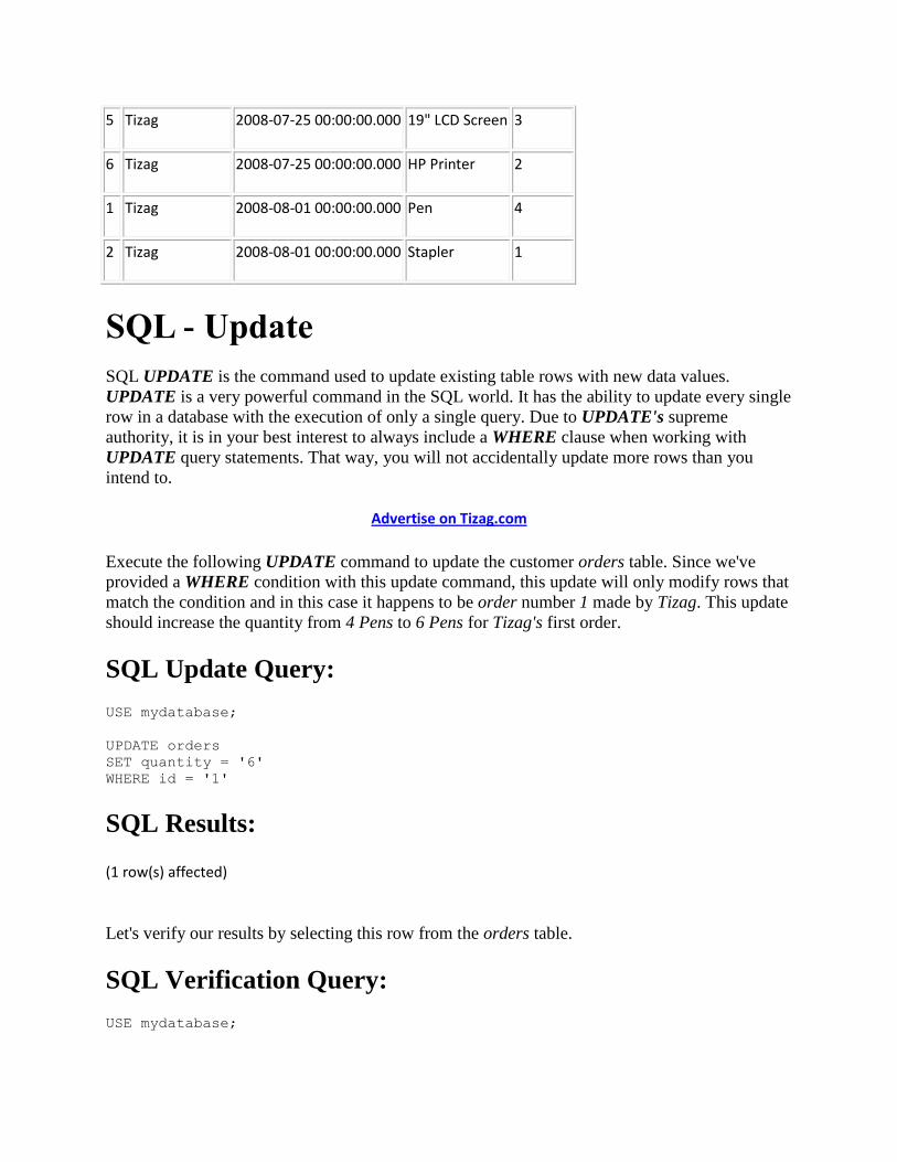
SQL - Update
SQL UPDATE is the command used to update existing table rows with new data values.
UPDATE is a very powerful command in the SQL world. It has the ability to update every single
row in a database with the execution of only a single query. Due to UPDATE's supreme
authority, it is in your best interest to always include a WHERE clause when working with
UPDATE query statements. That way, you will not accidentally update more rows than you
intend to.
Advertise on Tizag.com
Execute the following UPDATE command to update the customer orders table. Since we've
provided a WHERE condition with this update command, this update will only modify rows that
match the condition and in this case it happens to be order number 1 made by Tizag. This update
should increase the quantity from 4 Pens to 6 Pens for Tizag's first order.
SQL Update Query:
USE mydatabase;
UPDATE orders
SET quantity = '6'
WHERE id = '1'
SQL Results:
(1 row(s) affected)
Let's verify our results by selecting this row from the orders table.
SQL Verification Query:
USE mydatabase;
Page 33
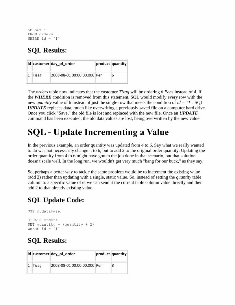
SELECT *
FROM orders
WHERE id = '1'
SQL Results:
id customer day_of_order product quantity
1 Tizag 2008-08-01 00:00:00.000 Pen 6
The orders table now indicates that the customer Tizag will be ordering 6 Pens instead of 4. If
the WHERE condition is removed from this statement, SQL would modify every row with the
new quantity value of 6 instead of just the single row that meets the condition of id = "1". SQL
UPDATE replaces data, much like overwriting a previously saved file on a computer hard drive.
Once you click "Save," the old file is lost and replaced with the new file. Once an UPDATE
command has been executed, the old data values are lost, being overwritten by the new value.
SQL - Update Incrementing a Value
In the previous example, an order quantity was updated from 4 to 6. Say what we really wanted
to do was not necessarily change it to 6, but to add 2 to the original order quantity. Updating the
order quantity from 4 to 6 might have gotten the job done in that scenario, but that solution
doesn't scale well. In the long run, we wouldn't get very much "bang for our buck," as they say.
So, perhaps a better way to tackle the same problem would be to increment the existing value
(add 2) rather than updating with a single, static value. So, instead of setting the quantity table
column to a specific value of 6, we can send it the current table column value directly and then
add 2 to that already existing value.
SQL Update Code:
USE mydatabase;
UPDATE orders
SET quantity = (quantity + 2)
WHERE id = '1'
SQL Results:
id customer day_of_order product quantity
1 Tizag 2008-08-01 00:00:00.000 Pen 8
Page 34
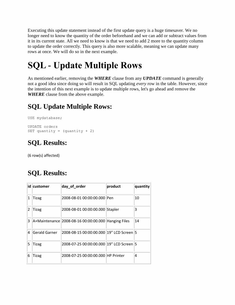
Executing this update statement instead of the first update query is a huge timesaver. We no
longer need to know the quantity of the order beforehand and we can add or subtract values from
it in its current state. All we need to know is that we need to add 2 more to the quantity column
to update the order correctly. This query is also more scalable, meaning we can update many
rows at once. We will do so in the next example.
SQL - Update Multiple Rows
As mentioned earlier, removing the WHERE clause from any UPDATE command is generally
not a good idea since doing so will result in SQL updating every row in the table. However, since
the intention of this next example is to update multiple rows, let's go ahead and remove the
WHERE clause from the above example.
SQL Update Multiple Rows:
USE mydatabase;
UPDATE orders
SET quantity = (quantity + 2)
SQL Results:
(6 row(s) affected)
SQL Results:
id customer day_of_order product quantity
1 Tizag 2008-08-01 00:00:00.000 Pen 10
2 Tizag 2008-08-01 00:00:00.000 Stapler 3
3 A+Maintenance 2008-08-16 00:00:00.000 Hanging Files 14
4 Gerald Garner 2008-08-15 00:00:00.000 19" LCD Screen 5
5 Tizag 2008-07-25 00:00:00.000 19" LCD Screen 5
6 Tizag 2008-07-25 00:00:00.000 HP Printer 4
Page 35
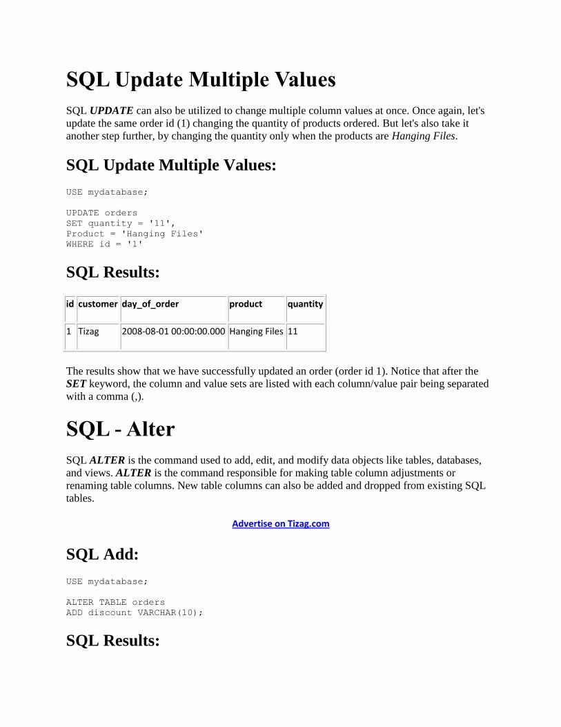
SQL Update Multiple Values
SQL UPDATE can also be utilized to change multiple column values at once. Once again, let's
update the same order id (1) changing the quantity of products ordered. But let's also take it
another step further, by changing the quantity only when the products are Hanging Files.
SQL Update Multiple Values:
USE mydatabase;
UPDATE orders
SET quantity = '11',
Product = 'Hanging Files'
WHERE id = '1'
SQL Results:
id customer day_of_order product quantity
1 Tizag 2008-08-01 00:00:00.000 Hanging Files 11
The results show that we have successfully updated an order (order id 1). Notice that after the
SET keyword, the column and value sets are listed with each column/value pair being separated
with a comma (,).
SQL - Alter
SQL ALTER is the command used to add, edit, and modify data objects like tables, databases,
and views. ALTER is the command responsible for making table column adjustments or
renaming table columns. New table columns can also be added and dropped from existing SQL
tables.
Advertise on Tizag.com
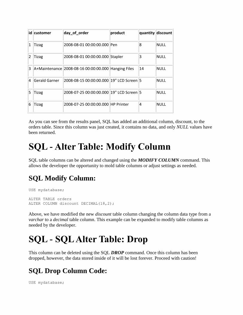
SQL Add:
USE mydatabase;
ALTER TABLE orders
ADD discount VARCHAR(10);
SQL Results:
Page 36
id customer day_of_order product quantity discount
1 Tizag 2008-08-01 00:00:00.000 Pen 8 NULL
2 Tizag 2008-08-01 00:00:00.000 Stapler 3 NULL
3 A+Maintenance 2008-08-16 00:00:00.000 Hanging Files 14 NULL
4 Gerald Garner 2008-08-15 00:00:00.000 19" LCD Screen 5 NULL
5 Tizag 2008-07-25 00:00:00.000 19" LCD Screen 5 NULL
6 Tizag 2008-07-25 00:00:00.000 HP Printer 4 NULL
As you can see from the results panel, SQL has added an additional column, discount, to the
orders table. Since this column was just created, it contains no data, and only NULL values have
been returned.
SQL - Alter Table: Modify Column
SQL table columns can be altered and changed using the MODIFY COLUMN command. This
allows the developer the opportunity to mold table columns or adjust settings as needed.
SQL Modify Column:
USE mydatabase;
ALTER TABLE orders
ALTER COLUMN discount DECIMAL(18,2);
Above, we have modified the new discount table column changing the column data type from a
varchar to a decimal table column. This example can be expanded to modify table columns as
needed by the developer.
SQL - SQL Alter Table: Drop
This column can be deleted using the SQL DROP command. Once this column has been
dropped, however, the data stored inside of it will be lost forever. Proceed with caution!
SQL Drop Column Code:
USE mydatabase;
Page 37
ALTER TABLE orders
DROP COLUMN discount;
SQL - Distinct
SQL SELECT DISTINCT is a very useful way to eliminate retrieving duplicate data reserved
for very specific situations. To understand when to use the DISTINCT command, let's look at a
real world example where this tool will certainly come in handy.
Advertise on Tizag.com
If you've been following along in the tutorial, we have created an orders table with some data
inside that represents different orders made by some of our very loyal customers over a given
time period. Let's pretend that we have just heard word from our preferred shipping agent that
orders made in August require no shipping charges, and we now have to notify our customers.
We do not want to send mailers to all of our customers, just the ones that have placed orders in
August. Also, we want to avoid retrieving duplicate customers as our customers may have placed
more than one order during the month of August.
We can write a very simple SQL query to extract this information from the orders table:
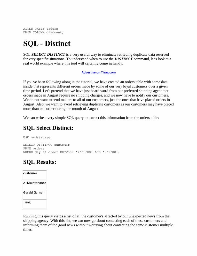
SQL Select Distinct:
USE mydatabase;
SELECT DISTINCT customer
FROM orders
WHERE day_of_order BETWEEN '7/31/08' AND '9/1/08';
SQL Results:
customer
A+Maintenance
Gerald Garner
Tizag
Running this query yields a list of all the customer's affected by our unexpected news from the
shipping agency. With this list, we can now go about contacting each of these customers and
informing them of the good news without worrying about contacting the same customer multiple
times.
Page 38
SQL - Subqueries
Subqueries are query statements tucked inside of query statements. Like the order of operations
from your high school Algebra class, order of operations also come into play when you start to
embed SQL commands inside of other SQL commands (subqueries). Let's take a look at a real
world example involving the orders table and figure out how to select only the most recent
order(s) in our orders table.
Advertise on Tizag.com
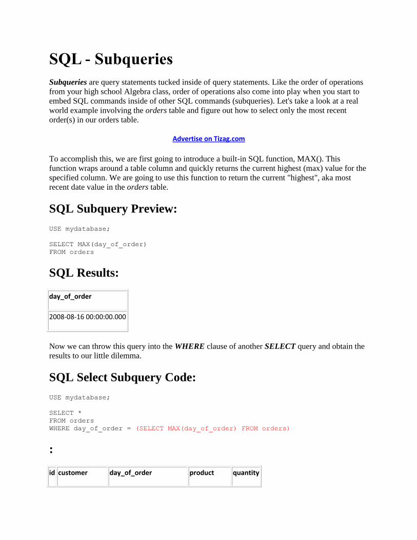
To accomplish this, we are first going to introduce a built-in SQL function, MAX(). This
function wraps around a table column and quickly returns the current highest (max) value for the
specified column. We are going to use this function to return the current "highest", aka most
recent date value in the orders table.
SQL Subquery Preview:
USE mydatabase;
SELECT MAX(day_of_order)
FROM orders
SQL Results:
day_of_order
2008-08-16 00:00:00.000
Now we can throw this query into the WHERE clause of another SELECT query and obtain the
results to our little dilemma.
SQL Select Subquery Code:
USE mydatabase;
SELECT *
FROM orders
WHERE day_of_order = (SELECT MAX(day_of_order) FROM orders)
:
id customer day_of_order product quantity
Page 39
3 A+Maintenance 2008-08-16 00:00:00.000 Hanging Files 14
This query is a dynamic query as it pulls current information and will change if a new order is
placed. Utilizing a subquery we were able to build a dynamic and robust solution for providing
us with current order information.
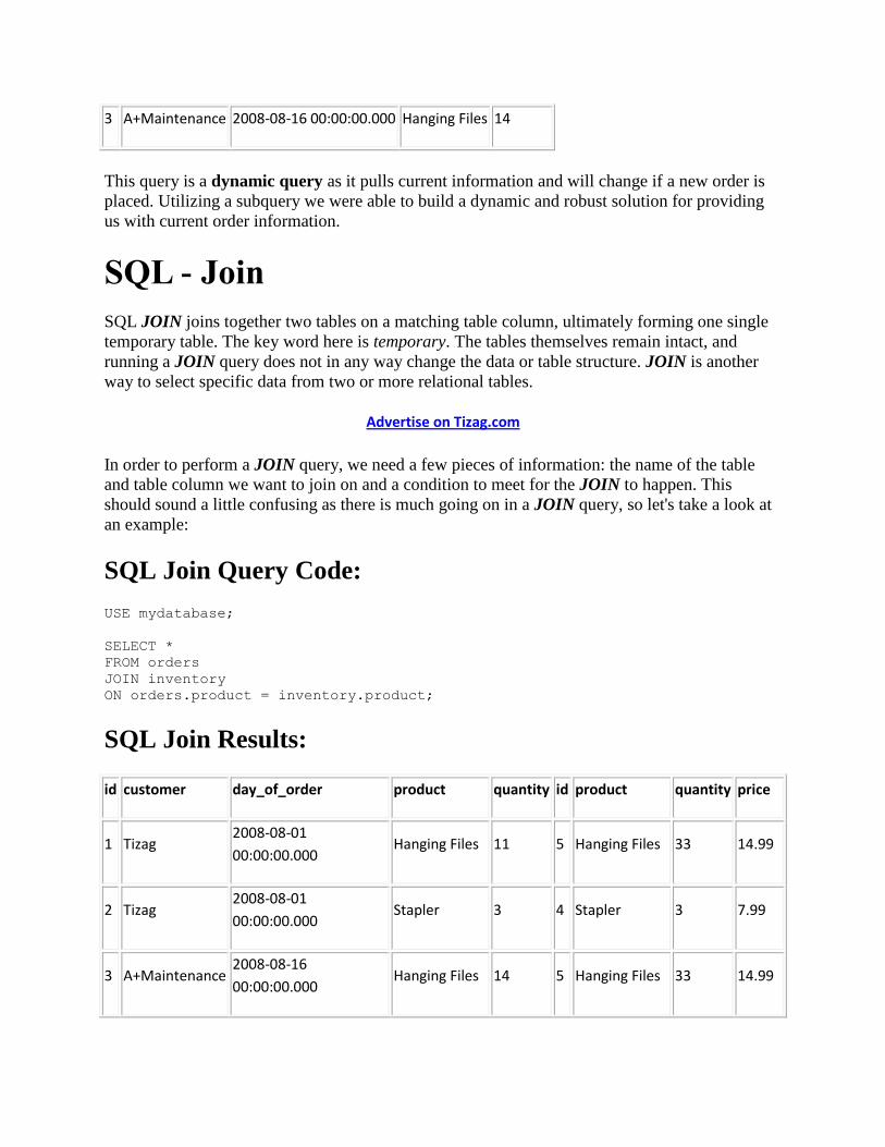
SQL - Join
SQL JOIN joins together two tables on a matching table column, ultimately forming one single
temporary table. The key word here is temporary. The tables themselves remain intact, and
running a JOIN query does not in any way change the data or table structure. JOIN is another
way to select specific data from two or more relational tables.
Advertise on Tizag.com
In order to perform a JOIN query, we need a few pieces of information: the name of the table
and table column we want to join on and a condition to meet for the JOIN to happen. This
should sound a little confusing as there is much going on in a JOIN query, so let's take a look at
an example:
SQL Join Query Code:
USE mydatabase;
SELECT *
FROM orders
JOIN inventory
ON orders.product = inventory.product;
SQL Join Results:
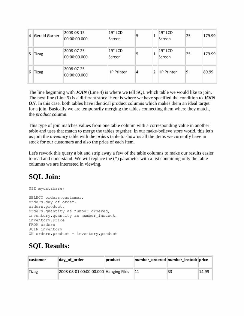
id customer day_of_order product quantity id product quantity price
1 Tizag 2008-08-01
00:00:00.000 Hanging Files 11 5 Hanging Files 33 14.99
2 Tizag 2008-08-01
00:00:00.000 Stapler 3 4 Stapler 3 7.99
3 A+Maintenance 2008-08-16
00:00:00.000 Hanging Files 14 5 Hanging Files 33 14.99
Page 40
4 Gerald Garner 2008-08-15
00:00:00.000
19" LCD
Screen 5 1
19" LCD
Screen 25 179.99
5 Tizag 2008-07-25
00:00:00.000
19" LCD
Screen 5 1
19" LCD
Screen 25 179.99
6 Tizag 2008-07-25
00:00:00.000 HP Printer 4 2 HP Printer 9 89.99
The line beginning with JOIN (Line 4) is where we tell SQL which table we would like to join.
The next line (Line 5) is a different story. Here is where we have specified the condition to JOIN
ON. In this case, both tables have identical product columns which makes them an ideal target
for a join. Basically we are temporarily merging the tables connecting them where they match,
the product column.
This type of join matches values from one table column with a corresponding value in another
table and uses that match to merge the tables together. In our make-believe store world, this let's
us join the inventory table with the orders table to show us all the items we currently have in
stock for our customers and also the price of each item.
Let's rework this query a bit and strip away a few of the table columns to make our results easier
to read and understand. We will replace the (*) parameter with a list containing only the table
columns we are interested in viewing.
SQL Join:
USE mydatabase;
SELECT orders.customer,
orders.day_of_order,
orders.product,
orders.quantity as number_ordered,
inventory.quantity as number_instock,
inventory.price
FROM orders
JOIN inventory
ON orders.product = inventory.product
SQL Results:
customer day_of_order product number_ordered number_instock price
Tizag 2008-08-01 00:00:00.000 Hanging Files 11 33 14.99
Page 41
Tizag 2008-08-01 00:00:00.000 Stapler 3 3 7.99
A+Maintenance 2008-08-16 00:00:00.000 Hanging Files 14 33 14.99
Gerald Garner 2008-08-15 00:00:00.000 19" LCD Screen 5 25 179.99
Tizag 2008-07-25 00:00:00.000 19" LCD Screen 5 25 179.99
Tizag 2008-07-25 00:00:00.000 HP Printer 4 9 89.99
Since we have one column in each table named the same thing (quantity), we used AS to modify
how these columns would be named when our results were returned. These results should be
more satisfying and easier to read now that we have removed some of the unnecessary columns.
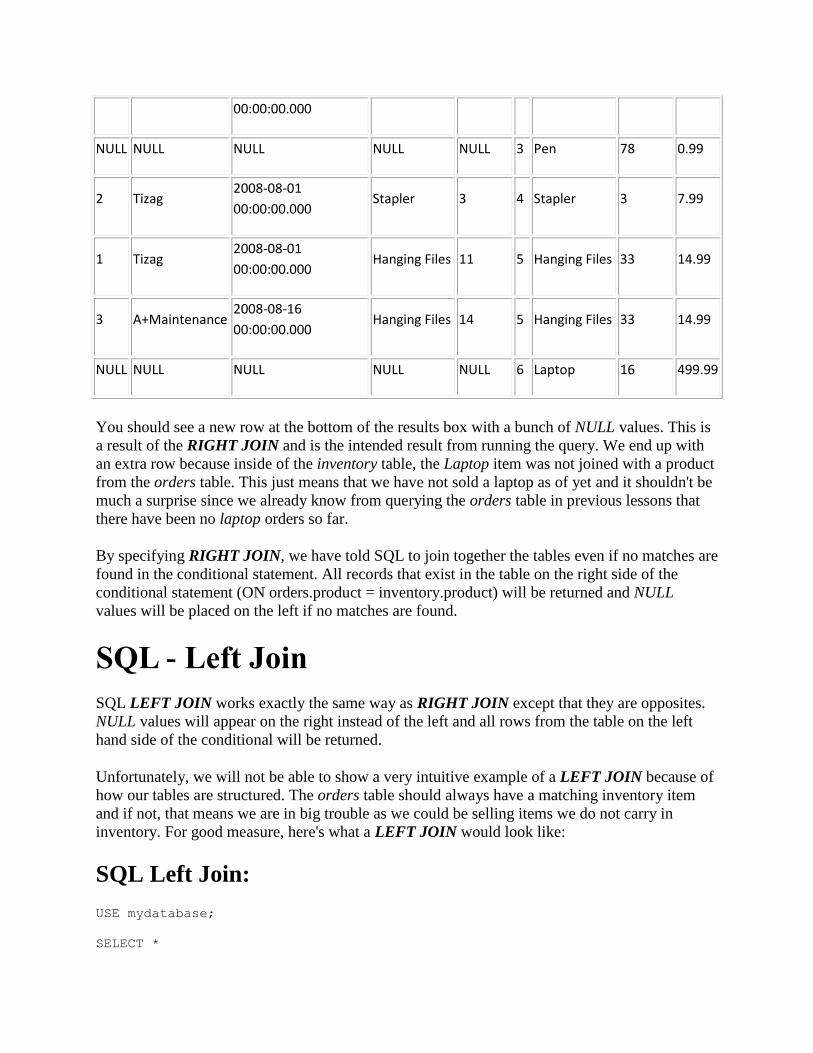
SQL - Right Join
RIGHT JOIN is another method of JOIN we can use to join together tables, but its behavior is
slightly different. We still need to join the tables together based on a conditional statement. The
difference is that instead of returning ONLY rows where a join occurs, SQL will list EVERY row
that exists on the right side, (The JOINED table).
SQL - Right Join:
USE mydatabase;
SELECT *
FROM orders
RIGHT JOIN inventory
ON orders.product = inventory.product
SQL Results:
id customer day_of_order product quantity id product quantity price
4 Gerald Garner 2008-08-15
00:00:00.000
19" LCD
Screen 5 1
19" LCD
Screen 25 179.99
5 Tizag 2008-07-25
00:00:00.000
19" LCD
Screen 5 1
19" LCD
Screen 25 179.99
6 Tizag 2008-07-25 HP Printer 4 2 HP Printer 9 89.99
Page 42
00:00:00.000
NULL NULL NULL NULL NULL 3 Pen 78 0.99
2 Tizag 2008-08-01
00:00:00.000 Stapler 3 4 Stapler 3 7.99
1 Tizag 2008-08-01
00:00:00.000 Hanging Files 11 5 Hanging Files 33 14.99
3 A+Maintenance 2008-08-16
00:00:00.000 Hanging Files 14 5 Hanging Files 33 14.99
NULL NULL NULL NULL NULL 6 Laptop 16 499.99
You should see a new row at the bottom of the results box with a bunch of NULL values. This is
a result of the RIGHT JOIN and is the intended result from running the query. We end up with
an extra row because inside of the inventory table, the Laptop item was not joined with a product
from the orders table. This just means that we have not sold a laptop as of yet and it shouldn't be
much a surprise since we already know from querying the orders table in previous lessons that
there have been no laptop orders so far.
By specifying RIGHT JOIN, we have told SQL to join together the tables even if no matches are
found in the conditional statement. All records that exist in the table on the right side of the
conditional statement (ON orders.product = inventory.product) will be returned and NULL
values will be placed on the left if no matches are found.
SQL - Left Join
SQL LEFT JOIN works exactly the same way as RIGHT JOIN except that they are opposites.
NULL values will appear on the right instead of the left and all rows from the table on the left
hand side of the conditional will be returned.
Unfortunately, we will not be able to show a very intuitive example of a LEFT JOIN because of
how our tables are structured. The orders table should always have a matching inventory item
and if not, that means we are in big trouble as we could be selling items we do not carry in
inventory. For good measure, here's what a LEFT JOIN would look like:
SQL Left Join:
USE mydatabase;
SELECT *
Page 43
FROM orders
LEFT JOIN inventory
ON orders.product = inventory.product
SQL JOIN is intended to bring together data from two tables to form a single larger table, and
often, it will paint a more detailed picture of what the data represents. By merging these two data
sets, we were able to peer into our database and ensure that each item ordered so far is in stock
and ready to be shipped to our customers.
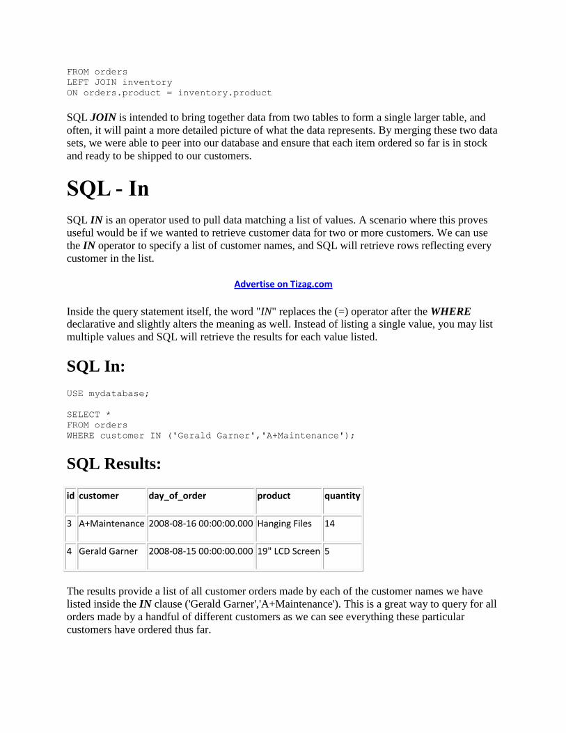
SQL - In
SQL IN is an operator used to pull data matching a list of values. A scenario where this proves
useful would be if we wanted to retrieve customer data for two or more customers. We can use
the IN operator to specify a list of customer names, and SQL will retrieve rows reflecting every
customer in the list.
Advertise on Tizag.com
Inside the query statement itself, the word "IN" replaces the (=) operator after the WHERE
declarative and slightly alters the meaning as well. Instead of listing a single value, you may list
multiple values and SQL will retrieve the results for each value listed.
SQL In:
USE mydatabase;
SELECT *
FROM orders
WHERE customer IN ('Gerald Garner','A+Maintenance');
SQL Results:
id customer day_of_order product quantity
3 A+Maintenance 2008-08-16 00:00:00.000 Hanging Files 14
4 Gerald Garner 2008-08-15 00:00:00.000 19" LCD Screen 5
The results provide a list of all customer orders made by each of the customer names we have
listed inside the IN clause ('Gerald Garner','A+Maintenance'). This is a great way to query for all
orders made by a handful of different customers as we can see everything these particular
customers have ordered thus far.
Page 44
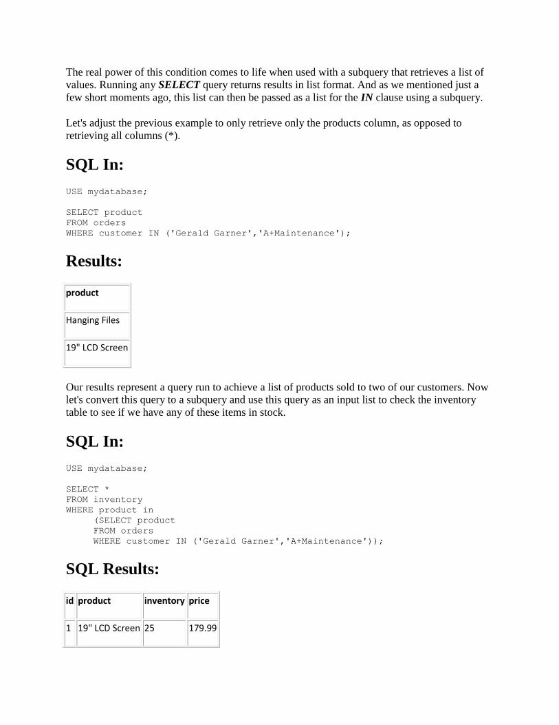
The real power of this condition comes to life when used with a subquery that retrieves a list of
values. Running any SELECT query returns results in list format. And as we mentioned just a
few short moments ago, this list can then be passed as a list for the IN clause using a subquery.
Let's adjust the previous example to only retrieve only the products column, as opposed to
retrieving all columns (*).
SQL In:
USE mydatabase;
SELECT product
FROM orders
WHERE customer IN ('Gerald Garner','A+Maintenance');
Results:
product
Hanging Files
19" LCD Screen
Our results represent a query run to achieve a list of products sold to two of our customers. Now
let's convert this query to a subquery and use this query as an input list to check the inventory
table to see if we have any of these items in stock.
SQL In:
USE mydatabase;
SELECT *
FROM inventory
WHERE product in
(SELECT product
FROM orders
WHERE customer IN ('Gerald Garner','A+Maintenance'));
SQL Results:
id product inventory price
1 19" LCD Screen 25 179.99
Page 45
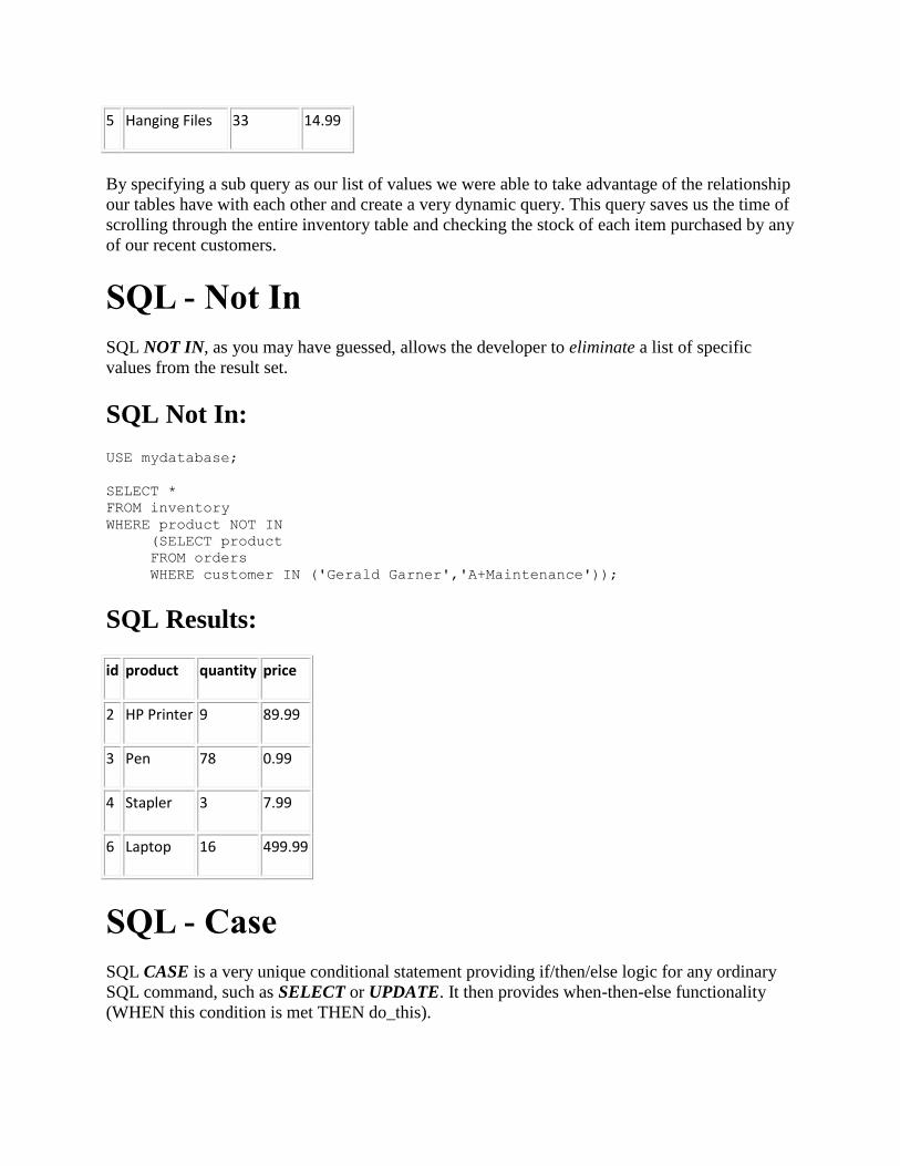
5 Hanging Files 33 14.99
By specifying a sub query as our list of values we were able to take advantage of the relationship
our tables have with each other and create a very dynamic query. This query saves us the time of
scrolling through the entire inventory table and checking the stock of each item purchased by any
of our recent customers.
SQL - Not In
SQL NOT IN, as you may have guessed, allows the developer to eliminate a list of specific
values from the result set.
SQL Not In:
USE mydatabase;
SELECT *
FROM inventory
WHERE product NOT IN
(SELECT product
FROM orders
WHERE customer IN ('Gerald Garner','A+Maintenance'));
SQL Results:
id product quantity price
2 HP Printer 9 89.99
3 Pen 78 0.99
4 Stapler 3 7.99
6 Laptop 16 499.99
SQL - Case
SQL CASE is a very unique conditional statement providing if/then/else logic for any ordinary
SQL command, such as SELECT or UPDATE. It then provides when-then-else functionality
(WHEN this condition is met THEN do_this).
Page 46
Advertise on Tizag.com
This functionality provides the developer the ability to manipulate the presentation of the data
without actually updating or changing the data as it exists inside the SQL table.
SQL Select Case Code:
USE mydatabase;
SELECT product,
'Status' = CASE
WHEN quantity > 0 THEN 'in stock'
ELSE 'out of stock'
END
FROM dbo.inventory;
SQL Results:
product Status
19" LCD Screen in stock
HP Printer in stock
Pen in stock
Stapler in stock
Hanging Files in stock
Laptop in stock
Using the CASE command, we've successfully masked the actual value of the product inventory
without actually altering any data. This would be a great way to implement some feature in an
online catalog to allow users to check the status of items without disclosing the actual amount of
inventory the store currently has in stock.
SQL - Case: Real World Example
As a store owner, there might be a time when you would like to offer sale prices for products.
This is a perfect opportunity to write a CASE query and alter the inventory sale prices at the
presentation level rather than actually changing the price inside of the inventory table. CASE
provides a way for the store owner to mask the data but still present it in a useful format.
Page 47
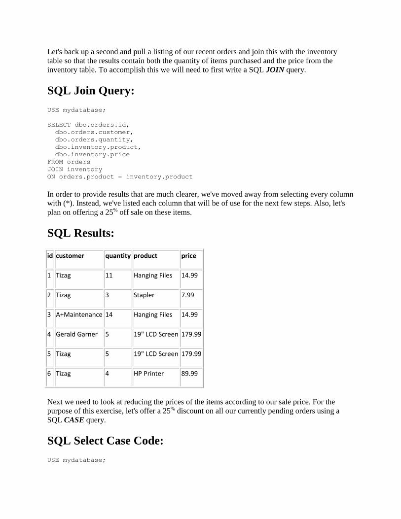
Let's back up a second and pull a listing of our recent orders and join this with the inventory
table so that the results contain both the quantity of items purchased and the price from the
inventory table. To accomplish this we will need to first write a SQL JOIN query.
SQL Join Query:
USE mydatabase;
SELECT dbo.orders.id,
dbo.orders.customer,
dbo.orders.quantity,
dbo.inventory.product,
dbo.inventory.price
FROM orders
JOIN inventory
ON orders.product = inventory.product
In order to provide results that are much clearer, we've moved away from selecting every column
with (*). Instead, we've listed each column that will be of use for the next few steps. Also, let's
plan on offering a 25% off sale on these items.
SQL Results:
id customer quantity product price
1 Tizag 11 Hanging Files 14.99
2 Tizag 3 Stapler 7.99
3 A+Maintenance 14 Hanging Files 14.99
4 Gerald Garner 5 19" LCD Screen 179.99
5 Tizag 5 19" LCD Screen 179.99
6 Tizag 4 HP Printer 89.99
Next we need to look at reducing the prices of the items according to our sale price. For the
purpose of this exercise, let's offer a 25% discount on all our currently pending orders using a
SQL CASE query.
SQL Select Case Code:
USE mydatabase;
Page 48
SELECT dbo.orders.id,
dbo.orders.customer,
dbo.orders.quantity,
dbo.inventory.product,
dbo.inventory.price,
'SALE_PRICE' = CASE
WHEN price > 0 THEN (price * .75)
END
FROM orders
JOIN inventory
ON orders.product = inventory.product
Multiplying the current price by .75 reduces the price by approximately 25%, successfully
applying the changes we would like to see but doing so without actually changing any data.
SQL Results:
id customer quantity product price SALE_PRICE
1 Tizag 11 Hanging Files 14.99 11.2425
2 Tizag 3 Stapler 7.99 5.9925
3 A+Maintenance 14 Hanging Files 14.99 11.2425
4 Gerald Garner 5 19" LCD Screen 179.99 134.9925
5 Tizag 5 19" LCD Screen 179.99 134.9925
6 Tizag 4 HP Printer 89.99 67.4925
The results speak for themselves as the records returned indicate a new table column with the
calculated sales price now listed at the end of each row.
Since SQL CASE offers a conditional statement (price > 0), it wouldn't take much more effort to
create some conditional statements based on how many products each customer had ordered and
offer different discounts based on the volume of a customer order.
For instance, as a web-company, maybe we would like to offer an additional 10% discount to
orders totaling more than $100. We could accomplish this in a very similar fashion.
SQL Results:
USE mydatabase;
Page 49
SELECT dbo.orders.id,
dbo.orders.customer,
dbo.orders.quantity,
dbo.inventory.product,
dbo.inventory.price,
'SALE_PRICE' = CASE
WHEN (orders.quantity * price) > 100 THEN (price * .65)
ELSE (price * .75)
END
FROM orders
JOIN inventory
ON orders.product = inventory.product
:
id customer quantity product price SALE_PRICE
1 Tizag 11 Hanging Files 14.99 9.7435
2 Tizag 3 Stapler 7.99 5.9925
3 A+Maintenance 14 Hanging Files 14.99 9.7435
4 Gerald Garner 5 19" LCD Screen 116.9935 134.9925
5 Tizag 5 19" LCD Screen 179.99 116.9935
6 Tizag 4 HP Printer 89.99 58.4935
With this query, we have now successfully reduced all orders by 25% and also applied an
additional 10% discount to any order totaling over $100.00.
In each of the examples above, SQL CASE has been utilized to perform presentation level
adjustments on data values and its versatility provides limitless results.
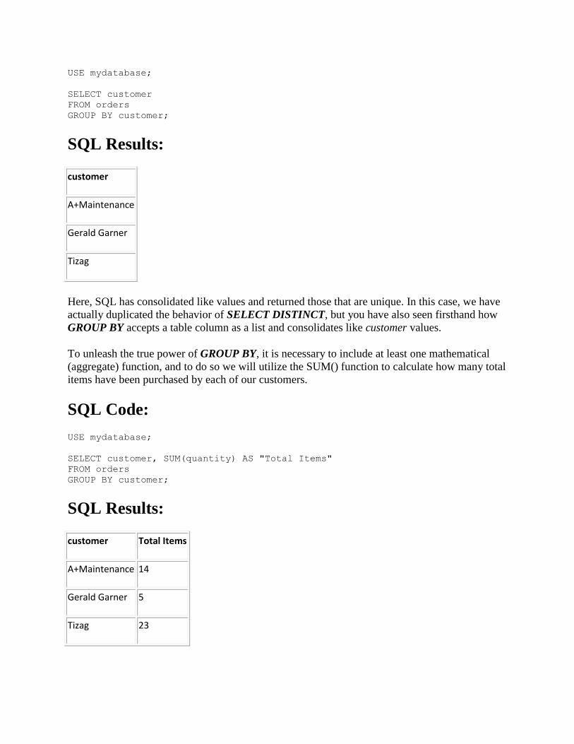
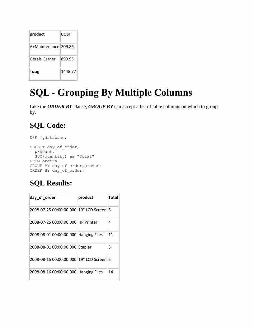
SQL - Group By
SQL GROUP BY aggregates (consolidates and calculates) column values into a single record
value. GROUP BY requires a list of table columns on which to run the calculations. At first, this
behavior will resemble the SELECT DISTINCT command we toyed with earlier.
Advertise on Tizag.com
SQL Group By:
Page 50
USE mydatabase;
SELECT customer
FROM orders
GROUP BY customer;
SQL Results:
customer
A+Maintenance
Gerald Garner
Tizag
Here, SQL has consolidated like values and returned those that are unique. In this case, we have
actually duplicated the behavior of SELECT DISTINCT, but you have also seen firsthand how
GROUP BY accepts a table column as a list and consolidates like customer values.
To unleash the true power of GROUP BY, it is necessary to include at least one mathematical
(aggregate) function, and to do so we will utilize the SUM() function to calculate how many total
items have been purchased by each of our customers.
SQL Code:
USE mydatabase;
SELECT customer, SUM(quantity) AS "Total Items"
FROM orders
GROUP BY customer;
SQL Results:
customer Total Items
A+Maintenance 14
Gerald Garner 5
Tizag 23
Page 51
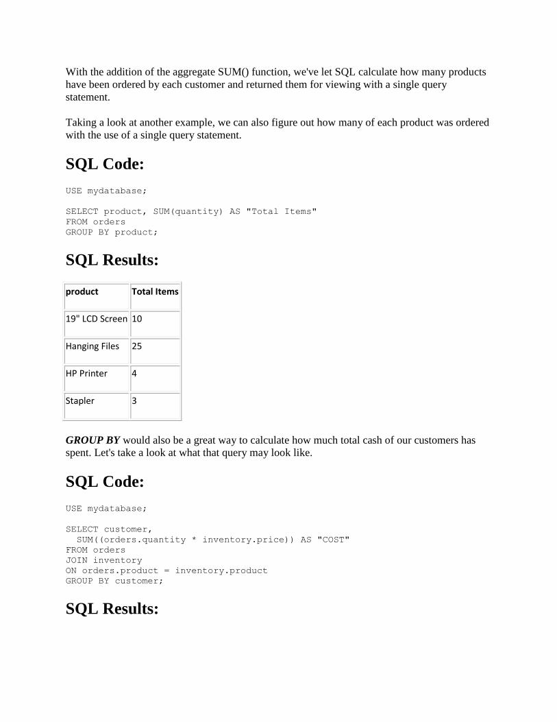
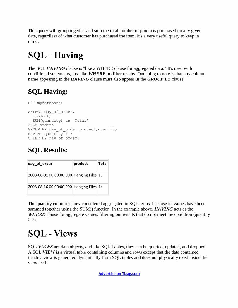
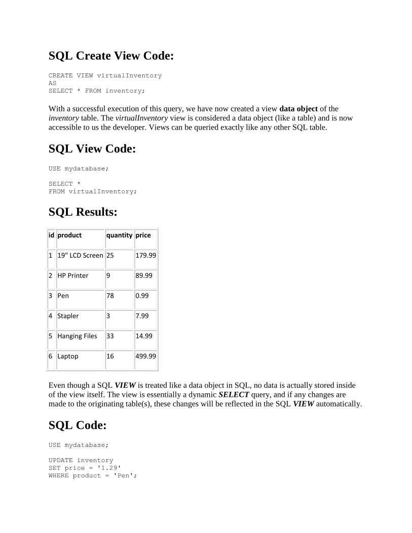
With the addition of the aggregate SUM() function, we've let SQL calculate how many products
have been ordered by each customer and returned them for viewing with a single query
statement.
Taking a look at another example, we can also figure out how many of each product was ordered
with the use of a single query statement.
SQL Code:
USE mydatabase;
SELECT product, SUM(quantity) AS "Total Items"
FROM orders
GROUP BY product;
SQL Results:
product Total Items
19" LCD Screen 10
Hanging Files 25
HP Printer 4
Stapler 3
GROUP BY would also be a great way to calculate how much total cash of our customers has
spent. Let's take a look at what that query may look like.
SQL Code:
USE mydatabase;
SELECT customer,
SUM((orders.quantity * inventory.price)) AS "COST"
FROM orders
JOIN inventory
ON orders.product = inventory.product
GROUP BY customer;
SQL Results:
Page 52
product COST
A+Maintenance 209.86
Gerals Garner 899.95
Tizag 1448.77
SQL - Grouping By Multiple Columns
Like the ORDER BY clause, GROUP BY can accept a list of table columns on which to group
by.
SQL Code:
USE mydatabase;
SELECT day_of_order,
product,
SUM(quantity) as "Total"
FROM orders
GROUP BY day_of_order,product
ORDER BY day_of_order;
SQL Results:
day_of_order product Total
2008-07-25 00:00:00.000 19" LCD Screen 5
2008-07-25 00:00:00.000 HP Printer 4
2008-08-01 00:00:00.000 Hanging Files 11
2008-08-01 00:00:00.000 Stapler 3
2008-08-15 00:00:00.000 19" LCD Screen 5
2008-08-16 00:00:00.000 Hanging Files 14
Page 53
This query will group together and sum the total number of products purchased on any given
date, regardless of what customer has purchased the item. It's a very useful query to keep in
mind.
SQL - Having
The SQL HAVING clause is "like a WHERE clause for aggregated data." It's used with
conditional statements, just like WHERE, to filter results. One thing to note is that any column
name appearing in the HAVING clause must also appear in the GROUP BY clause.
SQL Having:
USE mydatabase;
SELECT day_of_order,
product,
SUM(quantity) as "Total"
FROM orders
GROUP BY day_of_order,product,quantity
HAVING quantity > 7
ORDER BY day_of_order;
SQL Results:
day_of_order product Total
2008-08-01 00:00:00.000 Hanging Files 11
2008-08-16 00:00:00.000 Hanging Files 14
The quantity column is now considered aggregated in SQL terms, because its values have been
summed together using the SUM() function. In the example above, HAVING acts as the
WHERE clause for aggregate values, filtering out results that do not meet the condition (quantity
> 7).
SQL - Views
SQL VIEWS are data objects, and like SQL Tables, they can be queried, updated, and dropped.
A SQL VIEW is a virtual table containing columns and rows except that the data contained
inside a view is generated dynamically from SQL tables and does not physically exist inside the
view itself.
Advertise on Tizag.com
Page 54
SQL Create View Code:
CREATE VIEW virtualInventory
AS
SELECT * FROM inventory;
With a successful execution of this query, we have now created a view data object of the
inventory table. The virtualInventory view is considered a data object (like a table) and is now
accessible to us the developer. Views can be queried exactly like any other SQL table.
SQL View Code:
USE mydatabase;
SELECT *
FROM virtualInventory;
SQL Results:
id product quantity price
1 19" LCD Screen 25 179.99
2 HP Printer 9 89.99
3 Pen 78 0.99
4 Stapler 3 7.99
5 Hanging Files 33 14.99
6 Laptop 16 499.99
Even though a SQL VIEW is treated like a data object in SQL, no data is actually stored inside
of the view itself. The view is essentially a dynamic SELECT query, and if any changes are
made to the originating table(s), these changes will be reflected in the SQL VIEW automatically.
SQL Code:
USE mydatabase;
UPDATE inventory
SET price = '1.29'
WHERE product = 'Pen';
Page 55
Execute the following query to verify the results:
SQL Verification Query Code:
USE mydatabase;
SELECT *
FROM virtualInventory
WHERE product = 'Pen';
SQL Results:
id product quantity price
3 Pen 78 1.29
SQL - Drop View
Views can also be removed by using the DROP VIEW command.
SQL Drop View:
USE mydatabase;
DROP VIEW virtualInventory;
SQL - Dates
Date values are stored in date table columns in the form of a timestamp. A SQL timestamp is a
record containing date/time data, such as the month, day, year, hour, and minutes/seconds. It's
not much different from the standard date format.
Advertise on Tizag.com
Date Columns:
Column Type Format
time HH:MM:SS
Page 56
date YYYY-MM-DD
datetime YYYY-MM-DD HH:MM:SS
Date values are stored in the form of a timestamp, and SQL offers a built-in function called
GETDATE() that returns the current date in the form of a SQL timestamp.
SQL SELECT GETDATE():
USE mydatabase;
SELECT GETDATE();
Timestamp Result:
2004-06-22 10:33:11.840
SQL expects dates to be formatted as above but does offer some flexibility when working with
dates inside query statements. For instance, date values do not necessarily need to contain the
hour, minutes, and seconds values. SQL also accepts most traditional date formats such as
"MM/DD/YY" (ex: "01/01/06").
Using a built in function, ISDATE() we can do some testing on date values to see if they meet
the formatting requirements.
SQL Code:
USE mydatabase;
SELECT
ISDATE('8/24/08') AS "MM/DD/YY",
ISDATE('2004-12-01') AS "YYYY/MM/DD";
ISDATE() returns a 1 or a 0 indicating a true or false result. In this case, both formats are
acceptable date formats as a 1 value was returned.
SQL - Month(), Day(), Year()
The Month(), Day() and Year() functions all extract corresponding values from a given date.
SQL Year():
Page 57
USE mydatabase;
SELECT YEAR(GETDATE()) as "Year";
SELECT YEAR('8/14/04') as "Year";
SQL Month():
USE mydatabase;
SELECT MONTH(GETDATE()) as "Month";
SELECT MONTH('8/14/04') as "Month";
SQL Day():
USE mydatabase;
SELECT DAY(GETDATE()) as "Day";
SELECT DAY('8/14/04') as "Day";
Understanding timestamps and extracting pieces of dates is the first step in being able to perform
date calculations and work more in-depth with SQL Dates.
SQL - Datepart
DATEPART() is a SQL function used to extract all kinds of date information from timestamps,
and it is a function that is unique to Microsoft's SQL Server Application.
Advertise on Tizag.com
SQL Datepart:
USE mydatabase;
SELECT DATEPART(year, '2007-06-01') AS "Year";
SQL Results:
Year
2007
DATEPART() requires 2 parameters separated by a comma (,). The first parameter specifies
what type of date data will be extracted, and the second parameter is a timestamp value.
Page 58
SQL Datepart:
USE mydatabase;
SELECT DATEPART(year, '2007-06-01') AS "Year",
DATEPART(month, '2007-06-01') AS "Month",
DATEPART(day, '2007-06-01') AS "Day",
DATEPART(dayofyear, '2007-06-01') AS "DayofYear",
DATEPART(weekday, '2007-06-01') AS "Weekday";
SQL Results:
Year Month Day DayofYear Weekday
2007 6 1 152 6
Datepart Abbreviation Chart:
DatePart Abbreviation Example
year yy, yyyy DATEPART(yy, getdate())
quarter qq, q DATEPART(qq, getdate())
month mm, m DATEPART(mm, getdate())
dayofyear dy, y DATEPART(dy, getdate())
day dd, d DATEPART(dd, getdate())
week wk, ww DATEPART(wk, getdate())
weekday dw DATEPART(dw, getdate())
hour hh DATEPART(hh, getdate())
minute mi DATEPART(mi, getdate())
second ss DATEPART(ss, getdate())
millisecond ms DATEPART(ms, getdate())
Page 59
SQL - DateAdd()
DATEADD() is the SQL function used to add and increment date values. Hours, minutes,
months, and days can be added to any date value. In fact, dates can be added based on any type
of date part discussed in the SQL DATEPART() lesson.
Advertise on Tizag.com
SQL Code:
USE mydatabase;
SELECT DATEADD(year, 1, getdate()) AS "+1 Year";
SQL Results:
+1 Year
2009-06-31 00:00:00.000
This example shows how to use DATEADD() to take a specified date value and increment it by
the 'year' date part. By replacing the middle parameter with a negative value, we can utilize the
same DATEADD() function to subtract dates as well.
SQL Code:
USE mydatabase;
SELECT DATEADD(day,-1, '2006-06-01') AS "-1 Day";
SQL Results:
-1 Day
2006-05-31 00:00:00.000
In each example, SQL is able to perform a calculation on each date value based on a timestamp,
and after the calculation, a timestamp value returned. Also note that the date parameter can be
based on another SQL function or the result of a subquery.
SQL Code:
Page 60
USE mydatabase;
SELECT DATEADD(day,-30, (SELECT MAX(day_of_order) FROM orders)) AS "-30
Days";
SQL Results:
-30 Days
2008-07-17 00:00:00.000
Here we have now constructed a very useful, dynamic statement pulling the most current order
(MAX) in the orders table, and we've been able to subtract one day from that value. While this
information does not directly prove useful, if we take this query one step further and place this
statement in a WHERE as a subquery, we should be more satisfied with the results.
SQL Code:
USE mydatabase;
SELECT *
FROM orders
WHERE day_of_order >
(SELECT DATEADD(day,-30, (SELECT MAX(day_of_order) FROM orders)) AS "-30
Days");
SQL Results:
id customer day_of_order product quantity
1 Tizag 2008-08-01 00:00:00.000 Hanging Files 11
2 Tizag 2008-08-01 00:00:00.000 Stapler 3
3 A+Maintenance 2008-08-16 00:00:00.000 Hanging Files 14
4 Gerald Garner 2008-08-15 00:00:00.000 19" LCD Screen 5
5 Tizag 2008-07-25 00:00:00.000 19" LCD Screen 5
6 Tizag 2008-07-25 00:00:00.000 HP Printer 4
Page 61
By placing this calculated date in the WHERE clause, we were able to pull all the records that
have happened within 30 days of the most recent order (2008-07-17 00:00:00.000). We are able
to query the orders table and request this information with a dynamic query that will yield
different results as new orders are placed and time goes by.
SQL - Delete Command(s)
In the SQL world, databases, rows, and columns all have one thing in common: once a DELETE
statement has been executed successfully against them, the data they once contained is lost
forever! Be very careful with these commands and be sure to properly backup all data before
proceeding with any type of DELETE command(s).
Advertise on Tizag.com
SQL offers several ways to tackle data deletion. Here are the differences.
SQL Delete Commands:
DELETE - Deletes any number of rows from a data object.
DROP - Removes table columns, tables, and all data objects SQL applications.
TRUNCATE - Empties out data without removing the object itself.
SQL - Delete
DELETE queries work much like UPDATE queries and like UPDATE, it is much advised to
always use a WHERE condition when running any delete query or else you risk deleting too
much data.
SQL Delete Query:
USE mydatabase;
DELETE
FROM orders
WHERE customer = 'A+Maintenance';
SQL Results:
1 Row(s) affected
SQL - Truncate
Page 62
SQL TRUNCATE is the fastest way to remove all data from a SQL table, leaving nothing but an
empty shell. You might choose to use this command when all the data inside of a table needs to
be removed but you'd like the table column definitions to remain intact.
SQL Truncate Table Code:
USE mydatabase;
TRUNCATE TABLE orders;
NOTE: Executing the command above will empty your table data and you will lose this data
forever! If you plan on following along do not execute this query.
SQL - Drop
SQL DROP is another command that removes data from the data store. The DROP command
must be performed on SQL objects including databases, tables, table columns, and SQL views.
Dropping any of these objects removes them completely from your SQL application and all data
contained in any of the data objects dropped are lost forever.
SQL Drop Examples:
USE mydatabase;
DROP TABLE orders;
DROP DATABASE mydatabase;
DROP VIEW viewname;
DROP INDEX orders.indexname;
-- FOR USE WITH ALTER COMMANDS
DROP COLUMN column_name
DROP FOREIGN KEY (foreign_key_name)
The above example also includes the syntax to drop table columns and foreign keys. These items
are outlined in the SQL ALTER lesson.
SQL - Union
SQL UNION combines two separate SQL queries into one result set. A JOIN statement adds
additional table columns to a result set (horizontally), UNION combines row results from one
table with rows of another table (vertically).
Advertise on Tizag.com
Page 63
In order to perform a UNION the columns of table 1 must match those of table 2. This rule
ensures that the result set is consistent as rows are fetched by SQL.
For these next exercises we suggest creating two different tables that are identical in structure but
contain unique rows of data. We challenge you to do this by reviewing the SQL Create queries
and modifying them to create two brand new employee tables.
SQL Select Union Code:
USE mydatabase;
SELECT * FROM employees
UNION
SELECT * FROM employees2;
SQL Table:
ID Lastname Firstname Title
1 Johnson David crew
2 Hively Jessica crew
9 Hicks Freddy crew
10 Harris Joel crew
11 Davis Julie manager
101 Yazzow Jim crew
102 Anderson Craig crew
103 Carlson Kevin crew
104 Maines Brad crew
The result is a complete listing of every employee from the two tables, perhaps representing a list
of employees from two different departments.
The next example shows a more practical means of using a union clause. Here we will select all
of our employees from both tables and join them with our invoices table to generate a complete
list of sales from both stores on a given day.
Page 64
SQL Code:
SELECT employees.Lastname, employees.Firstname, invoices.Sale, invoices.Price
FROM employees
INNER JOIN invoices
ON employees.id = invoices.EmployeeID
UNION
SELECT employees2.Lastname, employees2.Firstname, invoices.Sale,
invoices.Price
FROM employees2
INNER JOIN invoices
ON employees2.id = invoices.EmployeeID;
SQL Table:
Lastname Firstname Sale Price
Johnson David HOT DOG 1.99
Hively Jessica LG SFT DRK 1.49
Davis Julie CK SLD 3.99
Yazzow Jim HOT DOG 1.99
Carlson Kevin LG SFT DRK 1.49
Here we combined a join query with the union clause to create one table.
SQL - Union All
UNION ALL selects all rows from each table and combines them into a single table. The
difference between UNION and UNION ALL is that UNION ALL will not eliminate duplicate
rows. Instead, it just pulls all rows from all tables fitting your query specifics and combines them
into a table.
SQL Code:
SELECT * FROM employees
UNION ALL
SELECT * FROM employees2;
SQL Table:
Page 65
ID Lastname Firstname Title
1 Johnson David crew
2 Hively Jessica crew
9 Hicks Freddy crew
10 Harris Joel crew
11 Davis Julie manager
101 Yazzow Jim crew
102 Anderson Craig crew
103 Carlson Kevin crew
11 Davis Julie manager
104 Maines Brad crew
SQL Code:
SELECT employees.Lastname, employees.Firstname, invoices.Sale, invoices.Price
FROM employees
INNER JOIN invoices
ON employees.id = invoices.EmployeeID
UNION ALL
SELECT employees2.Lastname, employees2.Firstname, invoices.Sale,
invoices.Price
FROM employees2
INNER JOIN invoices
ON employees2.id = invoices.EmployeeID;
SQL Table:
Lastname Firstname Sale Price
Johnson David HOT DOG 1.99
Hively Jessica LG SFT DRK 1.49
Page 66
Davis Julie CK SLD 3.99
11 Davis Julie manager
Yazzow Jim HOT DOG 1.99
Carlson Kevin LG SFT DRK 1.49
11 Davis Julie manager
11 Davis Julie manager
SQL - Syntax - (Speaking SQL)
Syntax, by definition, means the study of linguistic rules and patterns. Every programming
language, including SQL, must follow a unique set of guidelines termed syntax. Punctuation,
spaces, mathematical operators, and special characters have special meaning when used inside of
SQL commands and query statements. For example, each and every SQL command will end
with a semi colon (;).
Advertise on Tizag.com
Executing SQL commands that do not have proper syntax and formatting will result in a syntax
error. Syntax errors might be the most common and first error messages new SQL developers
will experience.
Let's now take a look at a very simple SQL command that will be used in just about every
example contained in this tutorial from here on out.
Sample SQL Command:
use mydatabase;
This command identifies a database as a target database, meaning that any SQL command or
query executed after this line will be run against the identified database. In this case, the database
'mydatabase' will be the target database. This is a good way to prevent mistakes and avoid
potential data loss and a good reason to include this command into each and every authored SQL
query.
SQL - Syntax: Capitalization and Spacing
Page 67
In some programming languages, capitalizing commands or excessive spacing may or may not
cause syntax code errors and cause the command to fail. SQL syntax is very loose when it comes
to capitalization and spacing, allowing a lot of room for the developer to decide on his/her own
preference in regards to capitalization and spacing.
Let's rewrite the same SQL command from the previous example and take advantage of SQL's
loose syntax characteristics.
Sample SQL Command:
USE
mydatabase;
The example above, though it does look different due to the capitalization and spacing, will yield
the same results as the first example.
SQL - Syntax: Building good habits
While coding in any language, it is important to develop good, consistent habits and maintain
clean code. Clean code allows another SQL developer to step right in where you have left off
without missing a beat. A developer with diligent coding habits will prevent many syntax errors
before executing his/her scripts and also will be able to detect possibly syntax problems before
they cause problems in a SQL Command.
Good habits include:
Consitency
Clean and Concise
Use of Comments (more on this later)
Scalability
Coding in any language is as much of an art form as authoring best selling novels and stories.
Take pride in doing so and always do your best to follow good coding habits.
SQL - Data Types
SQL data takes shape in several different forms, including character strings, numbers, file stores,
and dates. SQL developers call the shots as to what types of data will be stored inside each and
every table column when creating a SQL table. The developer must specify the column type of
each new SQL table column.
Advertise on Tizag.com
Page 68
Column types are synonymous with data types as the column type is what designates the type of
data that will be stored inside the column. In other words, a SQL data type is a label and a
guideline for SQL to understand what type of data is expected inside of each table column and
this identifies how SQL will interact with the stored data. Below, we will give you an overview
on the types of data that can be stored within a SQL table.
SQL - Numbers, Decimals, and Dates
Data Types:
Integers - (3, -17)
Point(Decimal) - (3.23415)
Date - (2004-06-22 10:33:11.840)
Storing numbers and decimals allows the developer to collect statistical data and create reports
based on the data contained inside the table. SQL can even perform mathematical calculations
against numeric data, providing endless number-crunching abilities.
In SQL, decimals are often referred to as point or floating-point numbers. These data types are
slightly different from the normal 'integer' data types.
For the most part, date values are treated like numbers and they can even be added together and
subtracted offering the developer the option to add days, months, or years together to create new
dates (more on this later). Additionally, specific data can be extracted from date values, allowing
the developer to pull specific date information from a date value like only the month number, the
year, or the day of the week.
SQL - Boolean Data
("TRUE" / "FALSE")
( 1 / 0 )
Boolean values are true/false types of data. A Boolean table column will contain either string
values of "True" and "False" or the numeric equivalent representation, with 0 being false and 1
being true.
SQL - Character Strings
Character Strings:
VARCHAR - ('Words or numbers')
Text - ('Once upon a time...')
Page 69
Strings range from a single word or character to large blocks of text including multiple
paragraphs and unique symbols. Set the table column type to VARCHAR or Text in order to
incorporate string data types into SQL tables.
SQL Server Table Column Types:
bigint Integer value (-9,223,372,036,854,775,808 -
9,223,372,036,854,775,807) 2^63
int smaller Integer value (-2,147,483,648) - (2,147,483,647) 2^31
smallint smaller Integer value (-32,768) - (32,767) 2^15
tinyint smaller Integer values 0 - 255 2^8
bit Integer data value (either 1 or 0 value) 1 or 0
decimal Decimal values from -10^38 - 10^38 10^38
numeric Decimal values from -10^38 - 10^38 10^38
money Money values (-922,337,203,685,477.5808) -
(922,337,203,685,477.5807) 2^63
smallmoney Smaller Money Values (-214,748.3648) - (214,748.3647) 2^31
datetime Date value (January 1, 1753) - (December 31, 9999)
smalldatetime Smaller Date Value (January 1, 1900) - (June 6, 2079)
timestamp Unique Number Value (updates when row is updated)
char Character String Value (max 8,000 characters)
varchar Character String Value maximum of 8,000 characters, unless otherwise
noted)
nchar Character String Value (max 4,000 characters)
nvarchar Character String Value (max 4,000 characters)
text Character String Value (max 2,147,483,647 characters) 2^31
ntext Character String Value (max 1,073,741,823 characters) 2^30
binary Binary Value (max 8,000 bytes)
varbinary Binary Value (max 8,000 bytes)
image Binary Value (max 2,147,483,647 bytes) 2^31
uniqueidentifier Global Unique ID (GUID)
SQL - Defaults and Null Values
NULL values are 'nothing' values. When a value is null, it means the value is empty and contains
no value -- not even '0'. NULLs are unique data types that are usually the default setting for all
table columns. When a SQL developer runs across a NULL value in a database, it is generally an
indication that this value is either new or has not been modified.
Page 70
The SQL developer may specify to allow or disallow the NULL values eliminating the
possibility of running across 'empty' table columns when creating a SQL table. If the developer
chooses not to allow NULL values he/she may specify a custom default value instead of the
NULL (nothing) value. Primary Key table columns do not allow NULL values since this
column's sole purpose is to be the unique identifier for a table column. Having a NULL unique
identifier would be similar to having a car license plate that is blank.
By default, NULL values are allowed on all newly created table columns meaning a table
column is allowed to be 'empty', except primary key columns. A NULL value is a special type of
value that can be tested for by most programming languages including SQL and can provide the
developer a means to 'test' and see if data exists or has been modified. As a new programmer you
may not fully understand the benefits a NULL value can bring, but with experience, you will
learn to hate/appreciate them.
SQL - Expressions
SQL Expressions are the pieces of a SQL query that compare values against other values or
perform arithmetic calculations. Expressions can be found inside of any SQL command usually
in the form of a conditional statement. In the SQL world, conditional statements and
expressions test or compare values against other values.
Advertise on Tizag.com
SQL - Boolean Expressions
Boolean expressions return rows (results) when a single value is matched.
SQL Boolean Expression:
USE mydatabase;
SELECT * FROM orders WHERE id = '1';
SQL Results:
id customer day_of_order product quantity
1 Tizag 2008-08-01 00:00:00.000 Pen 4
SQL - Numeric Expression
Numeric Expressions return a single numeric value instead of an entire row and usually perform
calculations.
Page 71
SQL Code:
USE mydatabase;
SELECT 15 + 4;
SQL Code:
USE mydatabase;
SELECT (15 / 5) * 10;
SQL Code:
USE mydatabase;
SELECT ((5+5) * (5+5));
Each of the examples above returns a numeric value which is displayed inside the results pane of
the SQL application. SQL also offers several built-in functions to perform what is known as
aggregate data calculations against a table or a specific table column.
AVG() -- Returns the average value of a stated column.
COUNT(*) -- Returns a count of the number of rows of table.
SUM() -- Returns the sum of a given column.
Using one of the following functions also returns a numeric value:
SQL Code:
USE mydatabase;
SELECT COUNT(*) AS "Number of Orders"
FROM orders;
SQL Code:
USE mydatabase;
SELECT SUM(quantity)AS "Total Number of Items Purchased"
FROM orders;
SQL Code:
USE mydatabase;
SELECT AVG(quantity) AS "Average Number of Items Purchased"
Page 72
FROM orders;
We can also combine these queries into a single query so that the results are viewable all at once.
SQL Code:
USE mydatabase;
SELECT COUNT(*) AS "Number of Orders",
SUM(quantity)AS "Total Number of Items Purchased",
AVG(quantity)AS "Average Number of Items Purchased"
FROM orders;
SQL - Date Expressions
As the name suggests, Date Expressions return date/time values.
GetDate() -- Returns the current date/time.
Current_Timestamp -- Returns the current timestamp.
Date expressions as you may have guessed, return date values. We will be taking a closer look at
date expressions later on in this tutorial. Stay tuned.
SQL Code:
USE mydatabase;
SELECT Current_Timestamp;
SELECT GETDATE();
SQL - Historical Information
In the '60's database software required the use of complex mainframe machines that were
difficult to maintain and run. Information technologists worked around the clock monitoring,
updating, and manually uncorrupting these machines.
Advertise on Tizag.com
Each mainframe ran different software from different manufacturers. IBM pulled ahead in
software development internationally with efforts of software aimed at database management.
The problem was that each mainframe ran a different type of "language".
Page 73
Enter SQL, the new standard for any database program: Structured Query Language. SQL
bridged the barriers between mainframes and allowed large corporations to network their efforts.
SQL was introduced in the 1970's and quickly gained international popularity. SQL allows a
programmer to tell a program exactly what data to retrieve and how to display it.
SQL - Under Development
Software at the time was still underdeveloped and several continuous problems plagued database
storage. Transactions happening at the same time were often combined, mixed together, or even
lost altogether. For instance, say two individuals made a deposit at exactly the same time from
two different locations. The software was unable to cope with this, and their bank transactions
were completely switched. Suzy deposited $10,000 while Joe withdrew $15. Because of the
faulty software Joe's withdrawal was posted on Suzy's account and Suzy's deposit was posted to
Joe's account.
Along came Relational Database Management Systems (RDBMS). This software is still being
used and is quite powerful. Relational databases allow developers to build relationships between
databases and tables. This provides tremendous opportunities for data management and is still
the favorite software used today. MySQL, SQL Server, DB2, and Oracle are all RDBMSs, and
each have a substantial hold in the market share to this day.
SQL - Platforms Applications
There are many, many different SQL applications in existence. A handful of platforms are
available for free and are the preferred choice among individuals and small businesses. Other
SQL platforms are designed with enterprise level customers in mind and are much more
expensive.
Advertise on Tizag.com
SQL Applications:
IBM's DB2
MySQL
PostgreSQL
Oracle
Microsoft's SQL Server
SQL - MySQL and PostgreSQL
MySQL and PostgreSQL are open source database programs rich in functionality and flexibility.
They are often the choice of web developers and small businesses simply because they are light-
Page 74
weight and are offered at the right price: free. Most open source software will also work across
multiple different operating systems, which is yet another benefit to small businesses.
SQL - SQL Server
Microsoft's SQL Server is steadily on the rise in the commercial world gaining popularity
slowly. This platform is only available to Windows users at this time, but offers its users very
user-friendly interface that is great for beginning SQL developers. A free trial version can be
downloaded at the Microsoft website.
SQL - DB2 and Oracle
By far the selection of choice for large corporations is either Oracle or DB2. Companies that
have large ties to IBM stick to their DB2 software whereas others have made the switch to
Oracle. These systems run on personal computers as well as large corporate mainframes and are
ideal for processing vast amounts of data at the enterprise level.
SQL - Commands
SQL commands are lines of SQL code that ask the SQL application to perform simple tasks
against with data inside of a database. Often we refer to commands as query statements or
scripts; all of these terms are synonymous. Most of the commands and statements you will see in
this tutorial are fairly standard and will work across multiple database applications despite the
fact this tutorial is aimed for the SQL Server Express user.
Advertise on Tizag.com
SQL commands are declarative sentences or 'orders' executed against a SQL database. The
typical command is comprised of several different components including clauses, functions,
expressions, or objects but the only required components are a SQL Clause and the data object (a
database or a database table).
SQL - Clauses
A SQL clause is the word or phrase that begins each SQL command statement and the single
most important component to any SQL command. Looking at the clause of any given SQL
command usually tells the SQL programmer what that particular command intends to do to the
database. For instance, a SELECT command begins with the SELECT clause and any level of
SQL programmer will recognize the SELECT query as a command selecting data from the
database.
Other SQL clauses include:
Page 75
Add
Drop
Create
Insert
Select
Update
Replace
Delete
SQL - Sample Commands
SQL Code:
SELECT getdate(); -- Selects the current (server) date and time.
CREATE DATABASE MyDatabase; -- Creates a database named Mydatabase;
INSERT INTO orders
-- Inserts data into a database table
VALUES('A+Maintenance','8/16/08','Hanging Files',12);
QL - Structure
The importance of building your tables correctly could be considered its own form of art.
Psychologists have even gone as far to say that those with the ability to organize their thoughts
and concepts well tend to be absolutely brilliant (ie Mozart, Einstein, DaVinci). A database is
only slightly different from the human brain and clear organization is a must, especially if large
quantities of people will be using the same database.
Advertise on Tizag.com
Designing the right database has a lot to do with what you need to accomplish. A database with
thousands and thousands or even millions of records requires a completely different solution than
a database that will only have a few hundred records. Think about the future and plan ahead.
SQL - Table Relationships
The key to a large database is having tables with material that can relate to one another. A great
example is the employee ID. Ever wonder or joke about being just another number to the
company. A lot of that has to do with the way they set up their database. A large company is
going to have a weekly payroll and a personal information table. They might be set up like the
following:
personal_info
Page 76
emp_id last_name first_name
0056 Mynce George
0097 Jenkins Fred
weekly_payroll
emp_id hours rateofpay
0056 37.5 27.00
0097 44.5 22.25
This set up proves useful in several ways. The tables are smaller, more compact, and precise,
allowing for maximum access speeds with each query. We can also moderate who has access to
each table, meaning that our accountant can have access to the payroll table, but not the personal
information table, eliminating security risks.
Relationship tables are the choice for high-traffic databases. There are countless security
advantages, faster query returns, and complete view customization (more on this later).
SQL - Predicates
SQL Predicates are found on the tail end of clauses, functions, and SQL expression inside of
existing query statements. We've actually already covered a few SQL predicates already and
most on this list should be familiar to you.
Advertise on Tizag.com
SQL Predicates:
AND
OR
LIKE
BETWEEN
AS
TOP(LIMIT)
SQL - Top
Page 77
SQL Top is used to limit the number of results returned by a query. The top command is
generally followed by a number that indicates the maximum number of results to return for a
given query.
SQL Code:
use mydatabase;
SELECT TOP 2 *
FROM orders
SQL Results:
id customer day_of_order product quantity
1 Tizag 2008-08-01 00:00:00.000 Pen 4
2 Tizag 2008-08-01 00:00:00.000 Stapler 3
SQL - Identifiers, Think SQL
As with any programming language, there are a few terms unique to SQL.
Advertise on Tizag.com
An Identifier is essentially a name of a database, table, or table column. As the creator of the
database, you are free to identify these objects as you please; we merely suggest you keep these
guidelines in mind when you do.
Develop your own unique naming scheme. -- Use terms that relate to one another and
will be easy to recognize apart from your code.
Be conscious of how long your names become. -- Especially be aware when the time
comes to name your columns.
Avoid names without meaning. -- Develop a working scheme that also has meaning
behind the names.
Be consistent. -- If you capitalize one table name, capitalize each table name; if you
choose to use abbreviations, make sure they do not have double meanings or ambiguous
meaning.
Develop a clear, concise schema, and stick to it as your database develops.
SQL - Literals
Page 78
Literal is a term for data types such as strings, numbers, or boolean values in SQL. These values
are not named by you the programmer; they just exist.
Literal Breakdown:
string literals
'This is a string value'
'5893 Moon River Dr.'
number literals
823
-4.5
3.387920
boolean literals
TRUE
FALSE
1
0