Oracle SQL Internals Handbook - Lagout SQL...Oracle SQL Internals Handbook ... SQL Index Tuning...

Oracle SQL Internals Handbook

Donald K. Burleson Joe Celko

Dave Ensor Jonathan Lewis

Dave Moore Vadim Tropashko

John Weeg

Oracle SQL Internals Handbook By Donald K. Burleson, Joe Celko, Dave Ensor, Jonathan Lewis, Dave Moore, Vadim Tropashko, John Weeg Copyright © 2003 by BMC Software and DBAzine. Used with permission. Printed in the United States of America. Series Editor: Donald K. Burleson Production Manager: John Lavender Production Editor: Teri Wade Cover Design: Bryan Hoff Printing History: August, 2003 for First Edition Oracle, Oracle7, Oracle8, Oracle8i and Oracle9i are trademarks of Oracle Corporation.

Many of the designations used by computer vendors to distinguish their products are claimed as Trademarks. All names known to Rampant TechPress to be trademark names appear in this text as initial caps. The information provided by the authors of this work is believed to be accurate and reliable, but because of the possibility of human error by our authors and staff, BMC Software, DBAZine and Rampant TechPress cannot guarantee the accuracy or completeness of any information included in this work and is not responsible for any errors, omissions or inaccurate results obtained from the use of information or scripts in this work. Links to external sites are subject to change; dbazine.com, BMC Software and Rampant TechPress do not control or endorse the content of these external web sites, and are not responsible for their content. ISBN: 0-9744355-1-1

Table of Contents Conventions Used in this Book .....................................................ix About the Authors ...........................................................................xi Foreword..........................................................................................xiii

Section One - SQL System Tuning

Chapter 1 - Parsing in Oracle SQL ........................................ 1 Parsing in SQL by Vadim Tropashko ............................................1

Chapter 2 - Are We Parsing Too Much? .............................. 10 Are We Parsing Too Much? by John Weeg................................ 10 What is Identical?............................................................................ 10 How Much CPU are We Spending Parsing? .............................. 11 Library Cache Hits.......................................................................... 12 Shared Pool Free Space ................................................................. 12 Cursors ............................................................................................. 13 Code.................................................................................................. 15 Do What You Can.......................................................................... 16

Chapter 3 - Oracle SQL Optimizer Plan Stability................ 17 Plan Stability in Oracle 8i/9i by Jonathan Lewis ....................... 17 The Back Door to the Black Box................................................. 17 Background / Overview................................................................ 18 Preliminary Setup............................................................................ 19 What Does the Application Want to Do? .................................. 20 What Do You Want the Application to Do? ............................. 21 From Development to Production.............................................. 26 Oracle 9 Enhancements ................................................................ 27 Caveats.............................................................................................. 28 Conclusion ....................................................................................... 29

Chapter 4 - SQL Tuning Using dbms_stats ........................ 31 Query Tuning Using DBMS_STATS by Dave Ensor.............. 31 Introduction..................................................................................... 31

Table of Contents iii

Test Environment .......................................................................... 31 Background...................................................................................... 32

Original Statement.......................................................................... 33 With Hash Join Hints ................................................................... 33

Oracle's Cost-based Optimizer..................................................... 34 CPU Cost ......................................................................................... 34 Key Statistics ................................................................................... 36 Other Factors .................................................................................. 36 Cursor Sharing ................................................................................ 37 Package DBMS_STATS................................................................ 38 Plan Stability .................................................................................... 38 Getting CBO to the Required Plan.............................................. 39 Localizing the Impact..................................................................... 40 Ensuring Outline Use .................................................................... 42 Postscript ......................................................................................... 42 Conclusions ..................................................................................... 43

Section Two - SQL Statement Tuning

Chapter 5 - Trees in SQL ..................................................... 44 Trees in SQL: Nested Sets and Materialized Path by Vadim Tropashko........................................................................................ 44 Adjacency List ................................................................................. 44 Materialized Path ............................................................................ 46 Nested Sets ...................................................................................... 48 Nested Intervals .............................................................................. 49 Partial Order .................................................................................... 50 The Mapping ................................................................................... 52 Normalization ................................................................................. 54 Finding Parent Encoding and Sibling Number ......................... 56 Calculating Materialized Path and Distance between nodes.... 57 The Final Test ................................................................................. 60

Chapter 6 - SQL Tuning Improvements.............................. 64

iv Oracle SQL Internals Handbook

SQL Tuning Improvements in Oracle 9.2 by Vadim Tropashko........................................................................................ 64 Access and Filter Predicates.......................................................... 64 V$SQL_PLAN_STATISTICS ..................................................... 69

Chapter 7 - Oracle SQL Tuning Tips .................................. 73 SQL tuning by Don Burleson....................................................... 73

Chapter 8 - Altering SQL Stored Outlines ........................... 75 Faking Stored Outlines in Oracle 9 by Jonathan Lewis............ 75 Review .............................................................................................. 75 The Changes.................................................................................... 76 New Features................................................................................... 81 Old Methods (1).............................................................................. 82 Old Methods (2).............................................................................. 84 The Safe Bet .................................................................................... 85 Conclusion ....................................................................................... 86 References........................................................................................ 87

Section Three - SQL Index Tuning

Chapter 9 - Using Bitmap Indexes with Oracle .................. 88 Understanding Bitmap Indexes by Jonathan Lewis .................. 88 Everybody Knows … .................................................................... 88 What Is a Bitmap Index? ............................................................... 89 Do Bitmaps Lock Tables? ............................................................. 91 Consequences of Bitmap Locks ................................................... 92 Problems with Bitmaps.................................................................. 94 Low Cardinality Columns.............................................................. 95 Sizing............................................................................................... 102 Conclusion ..................................................................................... 103 References...................................................................................... 104

Chapter 10 - SQL Star Transformations..............................105 Bitmap Indexes 2: Star Transformations by Jonathan Lewis 105 The Bitmap Star Transformation............................................... 107

Table of Contents v

Warnings ........................................................................................ 116 Conclusion ..................................................................................... 118 References...................................................................................... 119

Chapter 11 - Bitmap Join Indexes .......................................120 Bitmap Indexes 3 — Bitmap Join Indexes by Jonathan Lewis............................................................................................... 120 It's fantastic - What's the Problem............................................. 122 What Is a Bitmap Join Index?..................................................... 122 Issues .............................................................................................. 128 Conclusion ..................................................................................... 130 References...................................................................................... 131

Section Four - SQL Diagnostics

Chapter 12 - Tracing SQL Execution .................................132 Oracle_trace - the Best Built-in Diagnostic Tool? by Jonathan Lewis............................................................................................... 132 How Do I … ? .............................................................................. 132 What is oracle_trace ......................................................................... 133 Uses for oracle_trace ....................................................................... 134 Putting it All Together ................................................................. 134 Some Results ................................................................................. 139 Now What?.................................................................................... 139 The Future ..................................................................................... 141 Conclusion ..................................................................................... 142 Caveat ............................................................................................. 142 References...................................................................................... 142

Chapter 13 - Embedding SQL in Java & PL/SQL .............143 Java vs. PL/SQL: Where Do I Put the SQL? by Dave Moore ............................................................................................. 143 The Power of a Package .............................................................. 144 The Flexibility of Java .................................................................. 146 Performance .................................................................................. 147

vi Oracle SQL Internals Handbook

Benchmarks ................................................................................... 147

Environment ................................................................................. 148 The Tests........................................................................................ 148

Java:............................................................................................. 149 PL/SQL:.................................................................................... 149

Multiple Statements...................................................................... 149 Java:............................................................................................. 149 PL/SQL:.................................................................................... 150

Truncate ......................................................................................... 150 Java:............................................................................................. 150 PL/SQL:.................................................................................... 151

Benchmark Results ....................................................................... 151 Single Statement Results.............................................................. 151 Multiple Statements Results ........................................................ 152

Truncate Results ........................................................................... 152 Remote Results ............................................................................. 152

Conclusion ..................................................................................... 153

Chapter 14 - Matrix Transposition in Oracle SQL..............155 Matrix Transposition in SQL by Vadim Tropashko............... 155 Nesting and Unnesting ................................................................ 156 Integer Enumeration for Aggregate Dismembering ............... 157 User Defined Aggregate Functions ........................................... 159

Section Five - Advanced SQL

Chapter 15 - SQL with Keyword Searches ..........................163 Keyword Searches by Joe Celko................................................. 163

Chapter 16 - Using SQL with Web Databases ....................167 Web Databases by Joe Celko...................................................... 167

Chapter 17 - SQL and Calculated Columns ........................172 Calculated Columns by Joe Celko.............................................. 172 Introduction................................................................................... 172 Triggers........................................................................................... 173 INSERT INTO Statement.......................................................... 175

Table of Contents vii

UPDATE the Table ..................................................................... 176 Use a VIEW .................................................................................. 176

Index ...................................................................................178

viii Oracle SQL Internals Handbook

Conventions Used in this Book It is critical for any technical publication to follow rigorous standards and employ consistent punctuation conventions to make the text easy to read. However, this is not an easy task. Within Oracle there are many types of notation that can confuse a reader. Some Oracle utilities such as STATSPACK and TKPROF are always spelled in CAPITAL letters, while Oracle parameters and procedures have varying naming conventions in the Oracle documentation. It is also important to remember that many Oracle commands are case sensitive, and are always left in their original executable form, and never altered with italics or capitalization. Hence, all Rampant TechPress books follow these conventions: Parameters - All Oracle parameters will be lowercase italics.

Exceptions to this rule are parameter arguments that are commonly capitalized (KEEP pool, TKPROF), these will be left in ALL CAPS.

Variables – All PL/SQL program variables and arguments will also remain in lowercase italics (dbms_job, dbms_utility).

Tables & dictionary objects – All data dictionary objects are referenced in lowercase italics (dba_indexes, v$sql). This includes all v$ and x$ views (x$kcbcbh, v$parameter) and dictionary views (dba_tables, user_indexes).

SQL – All SQL is formatted for easy use in the code depot, and all SQL is displayed in lowercase. The main SQL terms (select, from, where, group by, order by, having) will always appear on a separate line.

Conventions Used in this Book ix

Programs & Products – All products and programs that are known to the author are capitalized according to the vendor specifications (IBM, DBXray, etc). All names known by Rampant TechPress to be trademark names appear in this text as initial caps. References to UNIX are always made in uppercase.

x Oracle SQL Internals Handbook

About the Authors Donald K. Burleson is one of the world’s top Oracle Database

experts with more than 20 years of full-time DBA experience. He specializes in creating database architectures for very large online databases and he has worked with some of the world’s most powerful and complex systems. A former Adjunct Professor, Don Burleson has written 15 books, published more than 100 articles in national magazines, serves as Editor-in-Chief of Oracle Internals and edits for Rampant TechPress. Don is a popular lecturer and teacher and is a frequent speaker at Oracle Openworld and other international database conferences.

Joe Celko was a member of the ANSI X3H2 Database Standards Committee and helped write the SQL-92 standards. He is the author of over 450 magazine columns and four books, the best known of which is SQL for Smarties (Morgan-Kaufmann Publishers, 1999). He is the Vice President of RDBMS at North Face Learning in Salt Lake City.

Dave Ensor is a Product Developer with BMC Software where his mission is to produce software solutions that automate Oracle performance tuning. He has been tuning Oracle for 13 years, and in total he has over 30 years active programming and design experience.

As an Oracle design and tuning specialist Dave built a global reputation both for finding cost-effective solutions to Oracle performance problems and for his ability to explain performance issues to technical audiences. He is co-author of the O'Reilly & Associates books Oracle Design and Oracle8 Design Tips.

About the Authors xi

Jonathan Lewis is a freelance consultant with more than 17 years experience in Oracle. He specializes in physical database design and the strategic use of the Oracle database engine. He authored Practical Oracle 8i - Building Efficient Databases published by Addison-Wesley, and is one of the best-known speakers on the UK Oracle circuit. Further details of his published papers, tutorials, and seminars can be found at http://www.jlcomp.demon.co.uk, which also hosts The Co-operative Oracle Users' FAQ for the Oracle-related Usenet newsgroups.

Dave Moore is a product architect at BMC Software in Austin, TX. He's also a Java and PL/SQL developer and Oracle DBA.

Vadim Tropashko works for Real World Performance group at Oracle Corp. Prior to that he was an application programmer and translated "The C++ Programming Language" by B.Stroustrup, 2nd edition into Russian. His current interests include SQL Optimization, Constraint Databases, and Computer Algebra Systems.

John Weeg has over 20 years of experience in information technology, starting as an application developer and progressing to his current level as an expert Oracle DBA. His focus for the past three years has been on performance, reliability, stability, and high availability of Oracle databases. Prior to this, he spent four years designing and creating data warehouses in Oracle. John can be reached at [email protected] or http://www.hesaonline.com/ dba/dba_services.shtml.

xii Oracle SQL Internals Handbook

Foreword The process of Oracle SQL tuning is a critical aspect of many Oracle databases. If the database fails to service its queries in an efficient manner, the system will bog down with additional disk I/O and unnecessary CPU and RAM consumption. Hence, it is a primary goal of all administrators to understand Oracle SQL statements. As Oracle has evolved into one of the world's most complex database management systems, it is imperative that all Oracle professionals understand the internal workings of Oracle's Cost Based Optimizer, and how it is used to choose the optimal access path to data. This book was created in order to meet that need. Drawing from some of the World's most highly respected experts on Oracle SQL tuning, this text explorers issues deep inside Oracle's Cost Based Optimizer, and provides insight into the successful optimization and tuning of SQL within your Oracle database. SQL Tuning is approached from five functional areas. In this text we will explore System Tuning, Statement Tuning, Index Tuning, Diagnostics, and Advance SQL. The first section delves into System Tuning by exploring such topics as parsing, SQL Optimizer Plan stability, and the dbms_stats utility. Section two, Statement Tuning, provides tips and tricks to writing more efficient SQL statements. Section three, Index Tuning, reviews bitmap indexes, star transformations, and the internals of bitmap joins. The next section on Diagnostics goes into tracing SQL statements, embedding SQL in Java and PL/SQL, and matrix

Foreword xiii

transposition. The text concludes with a discussion of advanced SQL topics such as keyword searches, using SQL with web databases, and calculated columns. The tips and tricks in this handbook come from some of the World’s more renown Oracle experts and we hope we have provided you with the tools and knowledge to write and optimize your SQL code.

xiv Oracle SQL Internals Handbook

1 Parsing in Oracle SQL CHAPTER

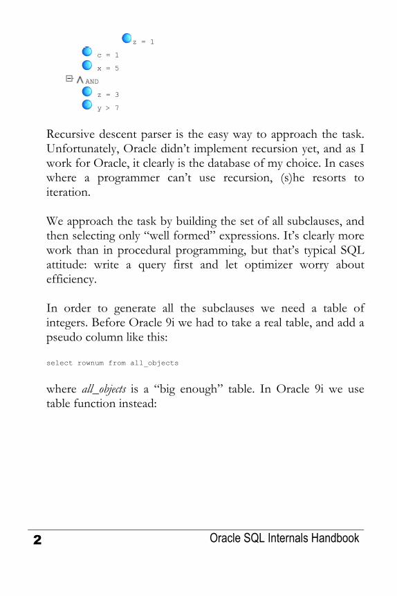
Parsing in SQL SQL is a high abstraction level language used exclusively as an interface to Relational Databases. Initially it lacked recursion, and, therefore, had a limited expression power, but eventually this construct has been added to the language. Here we'll explore how convenient SQL is for general-purpose programming. SQL programming is very unusual from procedural perspective: there is no explicit flow control, in general, and no loops, in particular, no variables either to apply operations to, or to store intermediate results into. SQL heavily leverages predicates instead. Our goal is writing a simple predicate expression parser in SQL. Given an expression like this, (((a=1 or b=1) and (y=3 or z=1)) and c=1 and x=5 or z=3 and y>7)

the parser should output a tree like this

OR

AND

AND

OR

a = 1

b = 1

OR

y = 3

Parsing in SQL 1

z = 1

c = 1

x = 5

AND

z = 3

y > 7

Recursive descent parser is the easy way to approach the task. Unfortunately, Oracle didn’t implement recursion yet, and as I work for Oracle, it clearly is the database of my choice. In cases where a programmer can’t use recursion, (s)he resorts to iteration. We approach the task by building the set of all subclauses, and then selecting only “well formed” expressions. It’s clearly more work than in procedural programming, but that’s typical SQL attitude: write a query first and let optimizer worry about efficiency. In order to generate all the subclauses we need a table of integers. Before Oracle 9i we had to take a real table, and add a pseudo column like this: select rownum from all_objects

where all_objects is a “big enough” table. In Oracle 9i we use table function instead:

2 Oracle SQL Internals Handbook

CREATE TYPE IntSet AS TABLE OF Integer; / CREATE or replace FUNCTION UNSAFE RETURN IntSet PIPELINED IS i INTEGER; BEGIN i := 0; loop PIPE ROW(i); i:=i+1; end loop; select rownum from TABLE(UNSAFE) where rownum < 1000

The UNSAFE function is rows producer and the above query is rows consumer. The producer generates a set of rows that fills in the buffer, and then pauses until all those rows are consumed by the query. The process repeats until either producer doesn’t have any rows or a consumer signals that it doesn’t need any more rows. The first possibility can be implemented as a function with a parameter that will determine when to exit the loop, but in our case it’s a consumer who signals producer to stop. It could also be viewed as if the "rowrun < 1000“ predicate were pushed down into the UNSAFE function. Be wary, however, because this predicate pushing works for rownum only. A cautious reader might want to convert the stop predicate into a parameter to the function, but in author’s opinion that solution would have less “declarative spirit.” The UNSAFE function is the procedural code that formally disqualifies the solution as being pure SQL. In my opinion, however, writing generic PL/SQL functions like integer sequence generator is very different from application specific PL/SQL code. Essentially, we extend RDBMS engine functionality, which is similar to what built-in SQL functions do.

Parsing in SQL 3

Now, with iteration abilities we have all the ingredients for writing the parser. Like traditional software practice we start by writing a unit test first: WITH src as( Select '(((a=1 or b=1) and (y=3 or z=1)) and c=1 and x=5 or z=3 and y>7)' exprfrom dual ), …

We refactored the "src" subquery into a separate view, because it would be used in multiple places. Oracle isn’t automatically refactoring the clauses that aren’t explicitly declared so. Next, we find all delimiter positions: ), idxs as ( select i from (select rownum i from TABLE(UNSAFE) where rownum < 4000) a, src where i<=LENGTH(EXPR) and (substr(EXPR,i,1)='(' or substr(EXPR,i,1)=' ' or substr(EXPR,i,1)=')' )

The “rownum<4000” predicate effectively limits parsing strings to 4000 characters only. In an ideal world this predicate wouldn’t be there. The subquery would produce rows indefinitely until some outer condition signaled that the task is completed so that producer could stop then. Among those delimiters, we are specifically interested in positions of all left brackets: ), lbri as( select i from idxs, src where substr(EXPR,i,1)='('

The right bracket positions view - rbri, and whitespaces – wtsp are defined similarly. All these three views can be defined directly, without introduction of idxs view, of course. However, it is much more efficient to push in predicates early, and deal with


idxs view which has much lower cardinality than select rownum i from TABLE(UNSAFE) where rownum < 4000. Now that we have indexed and classified all the delimiter positions, we’ll build a list of all the clauses, which begins and ends at the delimiter positions, and, then, filter out the irrelevant clauses. We extract the segment’s start and end points, first: ), begi as ( select i+1 x from wtsp union all select i x from lbri union all select i+1 x from lbri ), endi as ( -- [x,y) select i y from wtsp union all select i+1 y from rbri union all select i y from rbri

Note, that in case of brackets we consider multiple combinations of clauses - with and without brackets. Unlike starting point, which is included into a segment, the ending point is defined by an index that refers the first character past the segment. Essentially, our segment is what is called semiopen interval in math. Here is the definition: ), ranges as ( -- [x,y) select x, y from begi a, endi b where x < y

We are almost half way to the goal. At this point a reader might want to see what clauses are in the "ranges" result set. Indeed, any program development, including nontrivial SQL query writing, assumes some debugging. In SQL the only debugging facility available is viewing an intermediate result.

Parsing in SQL 5

Next step is admitting “well formed” expressions only: ), wffs1 as ( select x, y from ranges r -- -- bracket balance: where (select count(1) from lbri where i between x and y-1) = (select count(1) from rbri where i between x and y-1) -- -- eliminate '...)...(...' and (select coalesce(min(i),0) from lbri where i between x and y-1) <= (select coalesce(min(i),0) from rbri where i between x and y-1)

The first predicate verifies bracket balance, while the second one eliminates clauses where right bracket occurs earlier than left bracket. Some expressions might start with left bracket, end with right bracket and have well formed bracket structure in the middle, like (y=3 or z=1) , for example. We truncate those expressions to y=3 or z=1: ), wffs as ( select x+1 x, y-1 y from wffs1 w where (x in (select i from lbri) and y-1 in (select i from rbri) and not exists (select i from rbri where i between x+1 and y-2 and i < all(select i from lbri where lbri.i between x+1 and y-2)) ) union all select x, y from wffs1 w where not (x in (select i from lbri) and y-1 in (select i from rbri) and not exists (select i from rbri where i between x+1 and y-2 and i < all(select i from lbri where lbri.i between x+1 and y-2)) )

Now that the clauses don’t have parenthesis problems we are ready for parsing Boolean connectives. First, we are indexing all "or" tokens


), andi as ( select x i from wffs a, src s where lower(substr(EXPR, x, 3))='or'

and, similarly, all "and" tokens. Then, we identify all formulas that contain "or" connective ), or_wffs as ( select x, y, i from ori a, wffs w where x <= i and i <= y and (select count(1) from lbri l where l.i between x and a.i-1) = (select count(1) from rbri r where r.i between x and a.i-1)

and also "and" connective ), and_wffs as ( select x, y, i from andi a, wffs w where x <= i and i <= y and (select count(1) from lbri l where l.i between x and a.i-1) = (select count(1) from rbri r where r.i between x and a.i-1) and (x,y) not in (select x,y from or_wffs ww)

The equality predicate with aggregate count clause in both cases limits the scope to outside of the brackets. Connectives that are inside the brackets naturally belong to the children of this expression where they will be considered as well. The other important consideration is nonsymmetrical treatment of the connectives, because "or" has lower precedence than "and." All other clauses that don’t belong to either "or_wffs" or "and_wffs" category are atomic predicates: ), other_wffs as ( select x, y from wffs w minus select x, y from and_wffs w minus select x, y from or_wffs w

Given a segment - or_wffs, for example, generally, there would be a segment of same type enclosing it. The final step is selecting only maximal segments; essentially, only those are valid predicate formulas:

Parsing in SQL 7

), max_or_wffs as ( select distinct x, y from or_wffs w where not exists (select 1 from or_wffs ww where ww.x<w.x and w.y<=ww.y and w.i=ww.i) and not exists (select 1 from or_wffs ww where ww.x<=w.x and w.y<ww.y and w.i=ww.i)

and similarly defined max_and_wffs and max_other_wffs. These three views allow us to define ), predicates as ( select 'OR' typ, x, y, substr(EXPR, x, y-x) expr from max_or_wffs r, src s union all select 'AND', x, y, substr(EXPR, x, y-x) from max_and_wffs r, src s union all select '', x, y, substr(EXPR, x, y-x) from max_other_wffs r, src s

This view contains the following result set: TYP X Y EXPR

OR 2 64 ((a=1 or b=1) and (y=3 or z=1)) and c=1 and x=5 or z=3 and y>7 OR 4 14 a=1 or b=1 OR 21 31 y=3 or z=1

AND 2 49 ((a=1 or b=1) and (y=3 or z=1)) and c=1 and x=5 AND 3 32 (a=1 or b=1) and (y=3 or z=1) AND 2 49 z=3 and y>7

61 64 y>7 53 56 z=3 46 49 x=5 38 41 c=1 28 31 z=1 21 24 y=3 11 14 b=1 4 7 a=1

How would we build a hierarchy tree out of these data? Easy: the [X,Y) segments are essentially Celko’s Nested Sets. Oracle 9i added two new columns to the plan_table: access_predicates and filter_predicates. Our parsing technique allows


extending plan queries and displaying predicates as expression subtrees:

Parsing in SQL 9

Are We Parsing Too Much?

CHAPTER

2 Are We Parsing Too Much?

Each time we want to put on a sweater, we don't want to have to knit it. We want to just look in the cabinet and pull out the right one. Parsing a statement is like knitting that sweater. Parsing is one of our large CPU consumers, so we really want to do it only when necessary. To be as efficient as possible, we would have just one statement that is parsed once, and then all other executions find that statement already parsed. Of course, this isn't very useful, so we should try to parse as little as possible. A statement to be executed is checked to see if it is identical to one that has already been parsed and kept in memory. If so, then there is no reason to parse again.

What is Identical? Oracle has a list of checks it performs to see if the new statement is identical to one already parsed. 1. The new text string is hashed. You can see the hash values

in v$sqlarea. If the hash values match, then: 2. The text strings are compared. This includes spaces, case,

everything. If the strings are the same, then: 3. The objects referenced are compared. The strings might be

exactly the same, but are submitted under different


schemas, which could make the objects different. If the objects are the same, then:

4. The bind types of the bind variables must match. If we make it through all four checks, we can use the statement that is already parsed. So we really have two reasons, both over which we have control, for parsing a statement: that the statement is different from all others, or that it has aged out of memory. We will age out of memory if an old statement is pushed out by a new statement. So, we want to ensure that we have enough space to hold all the statements we will run.

How Much CPU are We Spending Parsing? To check how much of our CPU time is spent in parsing, we can run the following: column parsing heading 'Parsing|(seconds)' column total_cpu heading 'Total CPU|(seconds)' column waiting heading 'Read Consistency|Wait (seconds)' column pct_parsing heading 'Percent|Parsing' select total_CPU,parse_CPU parsing, parse_elapsed-parse_CPU waiting,trunc(100*parse_elapsed/total_CPU,2) pct_parsing from (select value/100 total_CPU from v$sysstat where name = 'CPU used by this session') ,(select value/100 parse_CPU from v$sysstat where name = 'parse time CPU) ,(select value/100 parse_elapsed from v$sysstat where name = 'parse time elapsed') ; Total CPU Parsing Read Consistency Percent (seconds) (seconds) Wait (seconds) Parsing ---------- ---------- ---------------- ---------- 5429326599 55780.65 17654.23 0

This shows that much less than one percent of our CPU seconds is spent parsing. It doesn't appear that we have a systematic re-parsing problem. Let's check further.

How Much CPU are We Spending Parsing? 11

Library Cache Hits The parsed statement is held in the library cache — another place to check. Are we finding what we look for in this cache? select sum(pins) executions,sum(reloads) cache_misses_while_executing, trunc(sum(reloads)/sum(pins)*100,2) pct from v$librarycache where namespace in ('TABLE/PROCEDURE','SQL AREA','BODY','TRIGGER'); EXECUTIONS CACHE_MISSES_WHILE_EXECUTING PCT ---------- ---------------------------- ---------- 397381658 2376530 .59

If we are missing more than one percent, then we need more space in our library cache. Of course, the only way to do add this space is to add space to the shared pool.

Shared Pool Free Space If we are running out of space in the shared pool, we will begin re-parsing statements that have aged off. column name format a25 column bytes format 999,999,999,999 select name,to_number(value) bytes from v$parameter where name ='shared_pool_size' union all select name,bytes from v$sgastat where pool = 'shared pool' and name = 'free memory'; NAME BYTES ------------------------- ---------------- shared_pool_size 167,772,160 free memory 23,148,312

It looks like we have plenty of space in the shared pool for new statements as they come. Let's continue the investigation.


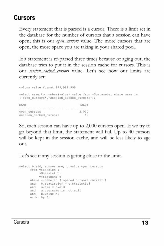
Cursors Every statement that is parsed is a cursor. There is a limit set in the database for the number of cursors that a session can have open; this is our open_cursors value. The more cursors that are open, the more space you are taking in your shared pool. If a statement is re-parsed three times because of aging out, the database tries to put it in the session cache for cursors. This is our session_cached_cursors value. Let's see how our limits are currently set: column value format 999,999,999 select name,to_number(value) value from v$parameter where name in ('open_cursors','session_cached_cursors'); NAME VALUE ------------------------- ------------ open_cursors 2,000 session_cached_cursors 40

So, each session can have up to 2,000 cursors open. If we try to go beyond that limit, the statement will fail. Up to 40 cursors will be kept in the session cache, and will be less likely to age out. Let's see if any session is getting close to the limit. select b.sid, a.username, b.value open_cursors from v$session a, v$sesstat b, v$statname c where c.name in ('opened cursors current') and b.statistic# = c.statistic# and a.sid = b.sid and a.username is not null and b.value >0 order by 3;

Cursors 13

SID USERNAME OPEN_CURSORS ---------- ------------------------------ ------------ 175 SYSTEM 1 150 ORADBA 2 236 ORADBA 14 28 ORADBA 105 205 ORADBA 110 107 ORADBA 124

There is no problem with the open cursor's limit. Let's check how often we are finding the cursor in the session cache: select a.sid,a.parse_cnt,b.cache_cnt,trunc(b.cache_cnt/a.parse_cnt*100,2) pct from (select a.sid,a.value parse_cnt from v$sesstat a, v$statname b where a.statistic#=b.statistic# and b.name = 'parse count (total)' and value >0) a ,(select a.sid,a.value cache_cnt from v$sesstat a, v$statname b where a.statistic#=b.statistic# and b.name ='session cursor cache hits') b where a.sid=b.sid order by 4,2; SID PARSE_CNT CACHE_CNT PCT ---------- ---------- ---------- ---------- 150 261 38 14.55 175 85 19 22.35 12 710399 344762 48.53 28 2661 1469 55.2 107 62762 36487 58.13 236 510 339 66.47 205 37379 24981 66.83 6 129022 91359 70.8 228 71 65 91.54

The sessions that are below 50 percent should be investigated. We see that SID 150 is finding the cursor less than 15 percent of the time. To see what he has parsed, we can use: select a.parse_calls,a.executions,a.sql_text from v$sqlarea a, v$session b where a.parsing_schema_id=b.schema# and b.sid=150 order by 1;

Because I get back 449 rows, I won't show these results in this article. However, the results do show me which statements are being re-parsed. These are similar based on the criteria above,


so we must be running out of cursor cache. It looks like we might want to increase this number. I will step it up slowly and watch the shared pool usage so I can increase the pool as necessary, too. Remember, you don't want to get so large that you cause paging at the system level.

Code We look pretty good at the system level. Now we can check the code that is being run to see if it passes the "identical" test: select a.parsing_user_id,a.parse_calls,a.executions,b.sql_text||'<' from v$sqlarea a, v$sqltext b where a.parse_calls >= a.executions and a.executions > 10 and a.parsing_user_id > 0 and a.address = b.address and a.hash_value = b.hash_value order by 1,2,3,a.address,a.hash_value,b.piece;

This returned 177 rows. Therefore, I have 177 statements that are parsed each time they are executed. Here is an example of two: PARSING_USER_ID PARSE_CALLS EXECUTIONS B.SQL_TEXT||'<' --------------- ----------- ---------- ---------------------------- 21 12698 12698 select sysdate from dual < 21 13580 13580 select sysdate from dual <

We see here that we have two statements that are identical except for the trailing space (that is why we concatenate the "<"). We also see that the statements are aging out of memory and therefore need to be re-parsed. This statement would benefit from being written exactly the same and from a higher value for session_cached_cursors, so it won't age out so quickly.

Code 15

To check for code that is similar you can look for many things. What I do most often is to look for the code being the same up to the first '('. select count(1) cnt,substr(sql_text,1,instr(SQL_text,'(')) string from v$sqlarea group by substr(SQL_text,1,instr(SQL_text,'(')) order by 1;

Again I get almost 200 rows back. An example is: CNT String --- ---------------------------------- 13 SELECT oradba.fn_physician_name(

To see these 13 statements we can use: Break on address skip 1 on hash_value select a.address,a.hash_value,b.sql_text||'<' from v$sqltext b ,(select a.address,a.hash_value from v$sqlarea a where a.sql_text like 'SELECT oradba.fn_physician_name(%') a where a.address = b.address and a.hash_value = b.hash_value order by a.address,a.hash_value,b.piece;

Now we want to look at each one to see why it is different than the others. I can see that these are different only in a single constant located in the "where" clause. If we made this a bind variable, we would be saving some time and space.

Do What You Can As a DBA, you can make sure there is nothing in the system definition that will cause additional parsing. You can also make code recommendations based on what you see. Hopefully, once you explain the benefits of the changes, they will even be made! Then you can spend less time knitting and get on with the business at hand.


Oracle SQL Optimizer Plan Stability

CHAPTER

3 Plan Stability in Oracle 8i/9i

Find out how you can use "stored outlines" to improve the performance of an application even when you can't touch the source code, change the indexing, or fiddle with the configuration.

Toolbox: For the purposes of experimentation, this article restricts itself to simple SQL and PL/SQL code running from an SQL*Plus session. The reader will need to have some privileges that a typical end-user would not normally be given, but otherwise need only be familiar with basic SQL. The article starts with Oracle 8i, but moves on to Oracle 9I, where several enhancements have appeared in the generation and handling of stored outlines.

The Back Door to the Black Box If you are a DBA responsible for a 3rd party application running on an Oracle database, you are sure to have experienced the frustration of finding a few extremely slow and costly SQL statements in the library_cache that would be really easy to tune -- if only you could add a few hints to the source code. Starting from Oracle 8.1 you no longer need to rewrite the SQL to add the hints -- you can make hints happen without touching the code. This feature is known as Stored Outlines, or Plan

Plan Stability in Oracle 8i/9i 17

Stability, and the concept is simple: you store information in the database that says: "if you see an SQL statement that looks like XXX then insert these hints in the following places>" This actually gives you three possible benefits. First of all, you can optimize that handful of expensive statements. Secondly, if there are other statements that Oracle takes a long time to optimize (rather than execute), you can save time and reduce contention in the optimization stage. Finally, it gives you an option for using the new cursor_sharing parameter without paying the penalty of losing optimum execution paths. There are a few issues to work around in Oracle 8 (largely eliminated in Oracle 9), but in general it is very easy to take advantage of this feature; and this article describes some of the things you can do.

Background / Overview To demonstrate how to make best use of stored outlines, we will start with a stored procedure with untouchable source code that (in theory) is running some extremely inefficient SQL. We will see how we can trap the SQL and details of its current execution path in the database, find some hints to improve the performance of the SQL, then make Oracle use our hints whenever that SQL statement is run in the future. In this demonstration, we will create a user, create a table in that user's schema, and create a procedure to access that table -- but just for fun we will use the wrap utility on the procedure so that we can't reverse-engineer the code. We will then set ourselves the task of tuning the SQL executed by that procedure.


The demonstration will assume that the stored outline infrastructure was installed automatically at database creation time.

Preliminary Setup Create a user with the privileges: create session, create table, create procedure, create any outline, and alter session. Connect as this user and run the following script to create a table: create table so_demo ( n1 number, n2 number, v1 varchar2(10) ) ; insert into so_demo values (1,1,'One'); create index sd_i1 on so_demo(n1); create index sd_i2 on so_demo(n2); analyze table so_demo compute statistics;

Now you need the code to create a procedure to access this table. Create a script called c_proc.sql containing the following: c_proc.sql

create or replace procedure get_value ( i_n1 in number, i_n2 in number, io_v1 out varchar2 ) as begin select v1 into io_v1 from so_demo where n1 = i_n1 and n2 = i_n2 ; end; /

Preliminary Setup 19

You could simply execute this script to build the procedure, of course -- but, just for effect, go to the operating system prompt and issue the command: wrap iname=c_proc.sql

The response should be: Processing c_proc.sql to c_proc.plb

Instead of executing the c_proc.sql script to generate the procedure, execute the incomprehensible c_proc.plb script and you will find that there is no trace of our target SQL statement anywhere in the user_source view.

What Does the Application Want to Do? Now that we have our pretend application we can run it, perhaps with sql_trace switched on, to see what happens. It won't be a great surprise to discover that the SQL performs a full tablescan to get the required data. In this little test, a full tablescan is probably the most efficient thing to do -- but let us assume that we have proved that we get the best performance when Oracle uses an execution path that combines our single column indexes using the and-equal option. How can we make this happen without hinting the code? With stored outlines, the answer is simple. There are actually several ways to achieve what I am about to do, so don't take this example as the definitive strategy. Oracle is always improving features to make life easier, and the mechanism described here will no doubt become obsolete in a future release.


What Do You Want the Application to Do? There are three stages to making Oracle do what we want: Start a new session and re-run the procedure, first telling

Oracle that we want it to trap each incoming SQL statement, along with information about the path that the SQL took. These "paths" are our first example of stored outlines. Create better stored outlines for any problem SQL

statements, and "exchange" the bad stored outlines with the good ones. Start a new session and tell Oracle to start using the new

stored outlines instead of using normal optimization methods when next it sees matching SQL; then run the procedure again.

We have to keep stopping and starting new sessions to ensure that existing cursors are not kept open by the pl/sql cache. Stored outlines are only generated and/or applied when a cursor is parsed, so we have to make sure that pre-existing similar cursors are closed. So start a session, and issue the command: alter session set create_stored_outlines = demo;

Then run a little anonymous block to execute the procedure, for example: declare m_value varchar2(10); begin get_value(1, 1, m_value); end; /

What Do You Want the Application to Do? 21

Then stop collecting execution paths (otherwise the next few bits of SQL that you run will also end up in the stored outline tables, making things harder to follow). alter session set create_stored_outlines = false;

To see the results of our activity, we can query the views that allow us to see details of the outlines that Oracle has created and stored for us: select name, category, used, sql_text from user_outines where category = 'DEMO'; NAME CATEGORY USED ------------------------------ ------------------------------ ------- SQL_TEXT ------------------------------------------------------------------------------ SYS_OUTLINE_020503165427311 DEMO UNUSED SELECT V1 FROM SO_DEMO WHERE N1 = :b1 AND N2 = :b2 select name, stage, hint from user_outline_hints where name = ' SYS_OUTLINE_020503165427311'; NAME STAGE HINT ------------------------------ ---------- ------------------------------ SYS_OUTLINE_020503165427311 3 NO_EXPAND SYS_OUTLINE_020503165427311 3 ORDERED SYS_OUTLINE_020503165427311 3 NO_FACT(SO_DEMO) SYS_OUTLINE_020503165427311 3 FULL(SO_DEMO) SYS_OUTLINE_020503165427311 2 NOREWRITE SYS_OUTLINE_020503165427311 1 NOREWRITE

We can see that there is a category named demo that has only one stored outline, and looking at the sql_text for that outline we can see something that is similar to, but not quite identical to, the SQL that exists in our original PL/SQL source. This is an important point as Oracle will only spot an opportunity to use a stored outline if the stored sql_text is a very close match to the SQL it is about to execute. In fact, under Oracle 8i the


SQL has to be an exact match, and this was initially a big issue when experimenting with stored outlines. You can see from the listing that stored outlines are just a set of hints that describe the actions Oracle took (or will take) when it runs the SQL. This plan uses a full tablescan -- and doesn't Oracle use a lot of hints to ensure the execution of something as simple as a full tablescan. Notice that a stored outline always belongs to a category; in this case the demo category, which we specified in our initial alter session command. If our original command had simply specified true rather than demo we would have found our stored outline in a category named default. Stored outlines also have names, and the names have to be unique across the entire database. No two outlines can have the same name, even if different users generated them. In fact outlines do not have owners, they only have creators. If you create a stored outline that happens to match a piece of SQL that I subsequently execute, then Oracle will apply your list of hints to my text -- even if those hints are meaningless in the context of my schema. (This gives us a couple of completely different options for faking stored outlines but that's another article). You may note that when Oracle is automatically generating stored outlines, the names have a simple format that includes a timestamp to the nearest millisecond. Moving on with the process of "tuning" our problem SQL, we decide that if we can inject the hint /*+ and_equal(so_demo, sd_i1, sd_i2) */ Oracle will use the execution path we want, so we now explicitly create a stored outline as follows: create or replace outline so_fix


for category demo on

select /*+ and_equal(so_demo, sd_i1, sd_i2) */ v1 from so_demo where n1 = 1 and n2 = 2;

This creates an explicitly named stored outline called so_fix in our demo category. We can see what the stored outline looks like by repeating our queries against user_outlines and user_outline_hints, with the predicate name = 'SO_FIX'. NAME CATEGORY USED ------------------------------ ------------------------------ --------- SQL_TEXT --------------------------------------------------------------------------- SO_FIX DEMO UNUSED select /*+ and_equal(so_demo, sd_i1, sd_i2) */ v1 from so_demo where n1 = 1 and n2 = 2 NAME STAGE HINT ------------------------------ ---------- -------------------------------- SO_FIX 3 NO_EXPAND SO_FIX 3 ORDERED SO_FIX 3 NO_FACT(SO_DEMO) SO_FIX 3 AND_EQUAL(SO_DEMO SD_I1 SD_I2) SO_FIX 2 NOREWRITE SO_FIX 1 NOREWRITE

Note, in particular that the line FULL(SO_DEMO) has been replaced with a line AND_EQUAL(SO_DEMO SD_I1 SD_I2), which is what we wanted to see. And now we have to "swap" the two stored outlines over. We want Oracle to use our new hint list whenever it sees the original text; and to do this, we have to cheat. The views user_outlines and user_outline_hints are generated from two tables (ol$ and ol$hints respectively) owned by the schema outln, and we are going to have to modify these tables directly; which means connecting to the database as outln, or using an account with the privilege to update the tables.


Fortunately, the outln tables do not have any enabled referential integrity constraints. Conveniently, the relationship between the ol$ (outlines) table and the ol$hints (hints) table is defined by the name of the outline (stored in column ol_name). So, checking names extremely carefully, we can exchange hints between stored outlines by swapping names on the ol$hints table, as follows: update outln.ol$hints set ol_name = decode( ol_name, 'SO_FIX','SYS_OUTLINE_020503165427311', 'SYS_OUTLINE_020503165427311','SO_FIX' ) where ol_name in ('SYS_OUTLINE_020503165427311','SO_FIX') ;

You may feel a little uncomfortable with hacking something that is so close to the Oracle kernel, especially given the comments in the manuals -- but this update is actually sanctioned in Metalink Note: 92202.1 Dated 5th June 2000. However, the note fails to mention that you may also need to do a second update to ensure that the numbers of hints associated with each stored outline stays consistent. If you fail to do this, you may find that some of your stored outlines become damaged or destroyed on an export/import cycle. update outln.ol$ ol1 set hintcount = ( select hintcount from ol$ ol2 where ol2.ol_name in ('SYS_OUTLINE_020503165427311',' SO_FIX') and ol2.ol_name != ol1.ol_name ) where ol1.ol_name in ('SYS_OUTLINE_020503165427311','SO_FIX') ;

Once the exchange is complete you can connect to a new session, tell it to start using stored outlines, re-run the


procedure and exit; again using sql_trace to check what Oracle actually does with the SQL. The mechanism to tell Oracle to use the (hacked) stored outline is the command: alter session set use_stored_outlines = demo;

Examining the trace file, you should find that the SQL now uses the and_equal path. (If you use TKPROF to process and explain the trace file you could well find that the output shows two contradictory paths. The first, correct, path should show the and_equal that took place, and the second path will probably show a full tablescan because the stored outline may not be invoked as TKPROF runs explain plan against the traced SQL).

From Development to Production Now that we have managed to create a single outline, we need to transfer it into the production environment. There are numerous little features of stored outlines that help us. For example, we could rename the stored outline, export it from development, import it to the production system, check that it still works properly on production in a 'test' category, and then move it into the production category. Useful commands are: alter outline SYS_OUTLINE_020503165427311 rename to AND_EQUAL_SAMPLE; alter outline AND_EQUAL_SAMPLE change category to PROD_CAT;

And to deal with exporting the outline from a development system to the production system, we can take advantage of the ability to add a where clause to an export parameter files, so we might have an export parameter file:


userid=outln/outln tables=(ol$, ol$hints, ol$nodes) # ol$nodes exists in v9 only file=so.dmp consistent=y # very important rows=yes query='where ol_name = ''AND_EQUAL_SAMPLE'''

Oracle 9 Enhancements There are many other details to consider when getting to grips with stored outlines, and in Oracle 8 there are some irritating and limiting features to what they can do and how they work. Fortunately, many of the issues are addressed in Oracle 9. The most trivial and obvious deficiency is that a stored outline in Oracle 8 can only be used if the stored text matches the incoming text exactly. In Oracle 9, there is a 'normalization' effect that relaxes this matching requirement; the texts are converted to capitals and have white space stripped before comparison. This increases the chance that marginally different pieces of SQL will be able to use the same stored outline. There are also some issues with more complex execution paths involving multiple query blocks -- Oracle Corp. has addressed these in Oracle 9 by introducing a third table in the outln schema called ol$nodes. This helps Oracle to break down the list of hints in ol$hints and cross-reference them with the correct sub-sections of the incoming SQL. This is, of course, a good thing. However, it may have some side effects on the strategy of swapping hints from one stored outline to another, as the ol$hints table has also acquired various details of text length and offsets. When upgrading to Oracle 9, it will become necessary to use alternative methods for manufacturing stored outlines, such as secondary schemas with specially crafted data sets, or missing indexes, or stored views with embedded hints being used to substitute for tables named in the text.

Oracle 9 Enhancements 27

Another feature of Oracle 9 is that there is more support for manufacturing stored outlines including the initial release of a package to allow you to edit stored outlines by direct access. More significantly though, there is an option to allow you to work on plans stored in a production system with an improved degree of safety. Although no-one likes to experiment on production, sometimes the production system is the only place that has the correct data distribution and volume to allow you to determine the optimum path for a piece of SQL. Under Oracle 9, you can create a private copy of the outln tables, and extract "public" stored outlines into them for "private" experimentation, without running the risk of accidentally making one of your private stored outlines visible to the end-user code. Personally I would consider this a last resort, but I could imagine that on occasion it might become a necessity. At a less dangerous level, if you have a full-scale UAT or development system, it is a feature that can be used to allow independence of testing

Caveats This article gives you enough information to start experimenting with stored outlines; but there are a few points you must be aware of before you start applying the technology to a production system.

First -- on Oracle 8i, the default password for outln (the schema that owns the tables used to hold stored outlines) has a well-known password, and the account has a very dangerous privilege. You must change the password on this account. On Oracle 9i, you should find that this account is locked.


Second -- the tables used to hold stored outlines are created in the system tablespace. For a production system, you could find that you are using a lot of space in the system tablespace when you start creating stored outlines. It is a good idea to move these tables, preferably to their own tablespace. Unfortunately, one of the tables includes a long column, so you will probably have to use exp/imp to move the tables to a new tablespace.

Third -- while stored outlines are extremely useful for solving critical performance problems, there is a cost involved. If stored outlines are activated, then Oracle checks whether a relevant stored outline exists every time a new statement is parsed. If there are large numbers of statements without a stored outline, then this overhead has to be balanced against the benefit you get on the few statements that do have stored outlines. However, this is only likely to be an issue on a system that has other, more serious, performance problems.

Conclusion Stored outlines can be of enormous benefit. When you can't modify the source code or the indexing strategy, a stored outline may be the only way to make a 3rd party application operate efficiently. Pushing the idea to the limit, if you still have to face the problem of switching a system from rule based to cost based optimization, then stored outlines may be your most cost-effective and risk-free option. If you need to get the best out of stored outlines, then Oracle 9 has several enhancements that allow it to cover more classes of

Conclusion 29

SQL, reduce the overheads, and allow you greater flexibility in testing, manipulating and installing stored outlines.


SQL Tuning Using dbms_stats

CHAPTER

4 Query Tuning Using DBMS_STATS

Introduction Increasingly enterprises are purchasing their mission-critical applications, whether these use Oracle or other data management software. Typically the licensing and support agreements for such applications seek to prevent the customer from reverse engineering or modifying the application in any way. Although such restrictions may be extremely sensible from a supplier's point of view, they can prevent an individual site from making changes that would result in valuable performance benefits. This paper describes the work performed to overcome a specific performance problem in a purchased application without having to resort to the obvious (but impossible) solution of modifying the application code.

Test Environment The experiments conducted during the preparation of this paper were performed on the author's laptop, a Compaq Armada M700 with 448 Mb of memory and a single 20 Gb hard disk partitioned into a FAT device for the operating system and an NTFS device for both the Oracle installation and the database files. The single processor is a Pentium III with a reputed clock speed of 833MHz; it certainly executed queries from the Oracle9i cache at impressive speed.

Query Tuning Using DBMS_STATS 31

The machine was running Microsoft Windows/2000 Professional with Service Pack 2, and Oracle9i Enterprise Edition release 9.0.1.0.1 with Oracle's pre-packaged "general purpose" database, although this was customized in a number of ways that did not affect the issues discussed in this paper.

Background BMC Software, Inc., uses Oracle as the dataserver for the majority of its administrative applications, and in most cases the applications themselves are proprietary and run under license. These applications are supported by their vendors but their administration is performed by BMC's internal IS department, which includes a specialist team of Oracle DBAs. As part of their role, this team monitors the resource consumption of the applications and the SQL statements being run on the data servers, and in the summer of 2001 one of the team identified that a very frequently executed statement form in one application was using excessive amounts of CPU time. The general form of this statement is select all ... from dm_qual_comp_sp dm_qual_comp, dm_qual_comp_rp dm_repeating where (dm_qual_comp.r_object_id in ('080f449c80009d10', '080f449c80009d13', ...)) and (dm_qual_comp.i_has_folder = 1 and dm_qual_comp.i_is_deleted = 0) and dm_repeating.r_object_id=dm_qual_comp.r_object_id;

It is worth noting that the SELECT list is not exceptional and is always the same. It has been omitted simply because of its length. The two objects in the FROM list are both join views, and any number of hexadecimal strings can appear in the IN list though typical forms of the statement contain between 6 and 20 items in the list. The use of the all qualifier and the


placement of the parentheses in the WHERE clause may tell us something about the level of Oracle experience of the person writing the statement, but neither is relevant to its performance. Because this statement was deemed to be using excessive CPU (around 250 msec per execution with several thousand executions per hour under peak load) the DBA used BMC's SQL Explorer for Oracle to capture an example of the statement from the shared pool, and started to experiment with various optimizer hints in an effort to improve performance. He quickly discovered that the query executed much more efficiently if it could be persuaded to use hash joins, and the TKPROF output from his experiments is summarized below.

Original Statement call count cpu elapsed disk query current rows ------- ----- ----- ------- ---- ----- ------- ---- Execute 1 0.00 0.01 0 0 0 0 Fetch 8 0.25 0.24 9 17675 0 92

With Hash Join Hints call count cpu elapsed disk query current rows ------- ----- ----- ------- ---- ----- ------- ---- Execute 1 0.01 0.01 0 0 0 0 Fetch 8 0.03 0.09 9 331 8 92

It should be noted that the TKPROF output has been slightly reformatted to fit on both the page in this paper and on the PowerPoint slides within the associated conference presentation. It is also worth noting that the production application runs on an 8 processor server, and therefore is entirely capable of handling well in excess of the 4,000 executions per hour that might at first sight appear to be the maximum possible service rate.

Background 33

The statements are clearly being built dynamically for each execution in order to include the literal values in the in list. BMC Software does not have access to the source code and was therefore unable to include the required hints directly. At this point, the author was contacted and asked whether or not he could think of a strategy that could allow IS to force this particular query form to perform hash joins without needing to change either the application code or the application schema. As discussed earlier, BMC Software does not have the ability to change the code. Schema changes, although technically feasible, would run the risk of being in violation of the relevant support agreement.

Oracle's Cost-based Optimizer This paper assumes the use of Oracle's Cost Based Optimizer (CBO). This is is used by the application in question rather than the older Rule Based Optimizer (RBO). The latter is still available under Oracle but is best viewed as being present solely for older applications that have been tuned to use it. All new development should assume the use of CBO. However until Oracle9i CBO does not use CPU resource as part of its cost equation, estimating instead what the Oracle documentation tends to refer to as I/O cost but which in reality equates more to "block visits for read." The difference between (nominal) disk reads and block visits is accounted for by Oracle's block caching mechanism, and is sometimes magnified by operating system or device controller caching.

CPU Cost Given that well-tuned Oracle applications are more likely to bottleneck on disk activity than on CPU, it might seem that basing CBO solely on I/O was an inspired decision.


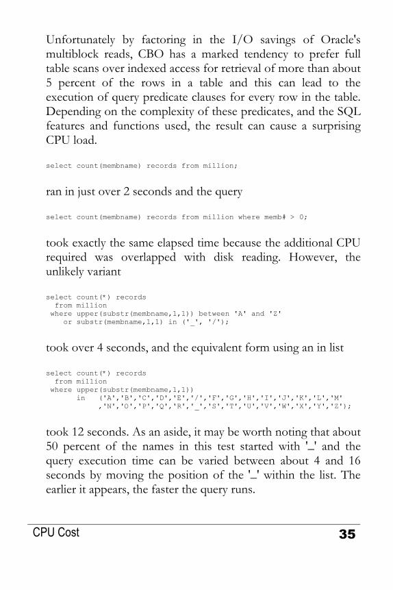
Unfortunately by factoring in the I/O savings of Oracle's multiblock reads, CBO has a marked tendency to prefer full table scans over indexed access for retrieval of more than about 5 percent of the rows in a table and this can lead to the execution of query predicate clauses for every row in the table. Depending on the complexity of these predicates, and the SQL features and functions used, the result can cause a surprising CPU load. select count(membname) records from million;

ran in just over 2 seconds and the query select count(membname) records from million where memb# > 0;

took exactly the same elapsed time because the additional CPU required was overlapped with disk reading. However, the unlikely variant select count(*) records from million where upper(substr(membname,1,1)) between 'A' and 'Z' or substr(membname,1,1) in ('_', '/');

took over 4 seconds, and the equivalent form using an in list select count(*) records from million where upper(substr(membname,1,1)) in ('A','B','C','D','E','/','F','G','H','I','J','K','L','M' ,'N','O','P','Q','R','_','S','T','U','V','W','X','Y','Z');

took 12 seconds. As an aside, it may be worth noting that about 50 percent of the names in this test started with '_' and the query execution time can be varied between about 4 and 16 seconds by moving the position of the '_' within the list. The earlier it appears, the faster the query runs.

CPU Cost 35

Key Statistics Once statistics have been gathered on a table and its indexes, CBO has available to it a number of values that it can use in estimating the number of database block visits that will be required. For tables these include the number of rows in the table, the number of blocks in the table and the average row length, and for indexes the number of keys in the index, the number of distinct keys, the number of blocks in the index leaf set, and the average number of both leaf blocks and data blocks per distinct key value. In addition, column value histograms can be captured, and these can be used to estimate the selectivity of specific key values. These statistics are not maintained in real time, but captured on demand using either the SQL command ANALYZE (now deprecated) or the supplied package DBMS_STATS, about which more later. We can see intuitively that with this kind of information available CBO should be able to make fairly accurate estimates of the number of block visits required to execute each discrete execution step, and at its simplest CBO works out for each of the possible approaches to the query which one generates the lowest total.

Other Factors Life is not, in reality, quite that simple as there are a number of other factors that influence how CBO works out the notional I/O cost. The simplest to understand is optimizer_mode, which is set at instance level but which can be over-ridden at session level. At a more complex level, a series of additional parameters, again settable at both index and session level, allow even more


variation in how the notional I/O cost is computed. For example the larger the value of the parameter sort_area_size, the more likely CBO is to elect to use a sort because large work areas reduce the disk traffic caused by sorting. Indeed, if the sort area is large enough then the sort can be performed entirely in memory with no I/O cost whatever. There is even a parameter optimizer_index_cost_adj that takes a value in the range 1 to 10,000 (default 100) and allows index usage to be made more or less attractive (low values make indexes more attractive). In some simple cases, we can get the changes that we need to the query plan simply by changing these parameters, though in many cases we will also need to change the statistics themselves.

Cursor Sharing The problem query that started the author's investigation contains a number of literal values supplied at run time and therefore the statement is almost certain to be slightly different each time that it is used. Oracle allows DBAs to get around this problem by setting the parameter cursor_sharing = FORCE (the default value is exact). With force set, any literal value in a SQL statement is replaced with a "bind variable" and thus each of select ORD# from ORDS where OTYPE = 'STD'; select ORD# from ORDS where OTYPE = 'GOV'; select ORD# from ORDS where OTYPE = 'STAFF';

will be executed as select ORD# from ORDS where OTYPE = :"SYS_B_0";

Cursor Sharing 37

This has both advantages and disadvantages. The main advantage is that the statement need only be parsed and optimized once, and for a simple query parsing can take longer than executing the query so the parse saving is significant. The main disadvantage is that if the selectivity of the key varies the optimizer will not be able to use a different approach for key values of different selectivity (in the example above 'STD' might select several hundred thousand rows whereas 'STAFF' might only select a few hundred). This problem is partly overcome in Oracle9i by having the optimizer to look at the "bind value" for the first execution, and to use that value to determine the execution path.

Package DBMS_STATS In Oracle9i, this Oracle supplied package contains about 35 procedures. Simple usage examples include: dbms_stats.gather_schema_stats ('SCOTT'); dbms_stats.delete_index_stats ('SCOTT', 'EMPPK'); dbms_stats.set_table_stats ('SCOTT', 'EMP' , numrows => 14 , numblks => 1 , avrglen => 48);

The procedures not only allow statistics to be gathered (and deleted) on tables, indexes, and column values but also allow these statistics to be inspected, changed, saved, and restored. Statistics can also be moved from one object to another and from an object in one database to an object in another database.

Plan Stability


This is a relatively recent feature of Oracle and sets out to ensure that the same plan is always used for a particular SQL

statement even if the optimizer parameters or the object statistics have been changed in the interim. The basic mechanism is to use the SQL statement CREATE OUTLINE to create a "stored outline" that contains both the SQL statement itself and a series of Oracle-generated hints that should always generate the same query plan as was generated when the outline was created. Creating outlines is quite simple, but managing them can quickly become a major problem if a large number are present within a single database. Because of the time constraints under which this paper was written, it has not been possible to include a full discussion of Plan Stability and the stored outline mechanism, but three observations may worth noting. First, the author's discussions with DBAs at user sites has persuaded him that the facility is little used and has yet to really impact on the consciousness of the Oracle community. Second, although its use adds a considerable CPU overhead to 'hard parses' this is rarely a significant problem because the feature is intended for high throughput transaction-based applications in which hard parses should be rare except in the period immediately after instance startup. Last, and rather surprisingly, the application of stored outlines to statements being parsed can only be enabled dynamically through alter system statements. It cannot be set in an INIT.ORA or SPFILE. This is apparently deliberate but the reasoning behind it is unknown to the author.

Getting CBO to the Required Plan The Oracle manual Oracle8i Designing and Tuning for Performance tells us that CBO uses hash joins when the two "row sources" to be joined together are large and of about the same order of

Getting CBO to the Required Plan 39

magnitude in size. Forcing the sample query to use hash joins was a relatively simple matter of adjusting the statistics on the four tables that underlie the two views in the query so that CBO felt that the conditions for using hash join were achieved. The table sizes in the production system (or at least in the statistics on the production system) were: Table Rows Blocks -------------------- -------- ------- DM_QUAL_COMP_R 250 1 DM_QUAL_COMP_S 125 1 DM_SYSOBJECT_R 398,790 1,392 DM_SYSOBJECT_S 271,966 9,313

It was realized early in the process that making small changes was invariably ineffective. However, by changing the table sizes to Table Rows Blocks -------------------- -------- ------- DM_QUAL_COMP_R 20,000 1,600 DM_QUAL_COMP_S 10,000 800 DM_SYSOBJECT_R 398,790 1,392 DM_SYSOBJECT_S 10,000 800

(and also making some changes to index selectivity to avoid index use) it was relatively easy to derive the required execution plan of three hash joins. However this had the obvious drawback that every query that accessed any one of these tables might now use a new execution plan because the statistics had been changed.

Localizing the Impact The easiest solution to preventing the changed statistics from affecting other queries was to create an outline for the query as soon as it had been tuned, and then to revert the statistics back to their previous values. This still had the effect of destabilizing


a production system during the trial and error process of deriving the required plan. The method adopted was to export both the production schema and the production statistics to a test instance using a combination of the DBMS_STATS package and Oracle's EXPort and IMPort utilities. Not a single row of application data was transferred, just the schema definition (using EXP with Table Data set to No) and the table and index statistics, by separately exporting the table statistics_table used by DBMS_STATS as both a destination to which to save object statistics and a source from which to restore them. With a production schema and production statistics on the test instance, and having taken some care to ensure that the optimizer environment was the same, we were able to conduct the trial and error process without affecting the production system. We already knew from hint-based tuning what plan we wanted, and once we achieved this an outline could be built for the statement and this outline transferred to the production system. The query being tuned was never actually executed on the test system. It was suggested to the author that under Oracle9i the supplied package DBMS_OUTLN_EDT could be used. In this scenario all that would be necessary, once the desired plan was known, would be to create an outline with the existing plan and then edit it to achieve the desired plan. Unfortunately a brief examination of the package showed that it was nowhere near powerful enough to achieve the required transformations.

Localizing the Impact 41

Ensuring Outline Use In order to ensure that the outline was used in production it was necessary not only to enable outlines, but also to set cursor_sharing = FORCE so that whatever the literal values that appeared in the statement, it would match the statement text stored in the outline table. Sadly, despite the success of the approach, it has not yet been deployed on the production system because of the need for this change, which has been deemed to require a performance test under production load using a test instance. This test has not yet been performed, and as the production server has sufficient CPU to cope with the inefficient query plan at current load volumes, IS have decided not to implement the solution until the load rises to the point at which the inefficiency starts to impact throughput.

Postscript It is worth noting that Jonathan Lewis has proposed a sneaky alternative approach to the method outlined above for creating the "preferred" stored outline for a query. In this simplified approach, an outline is first created for the original query and following tuning using hints, a second outline is created for the hinted version of the query. Once both outlines have been created, their hint entries in the table outln.ol$hints then (assuming sufficient privilege) these entries can be swapped over using simple update command of the general form update OUTLN.OL$HINTS set OL_NAME = decode(OL_NAME, 'VERSION1', 'VERSION2', 'VERSION1') where OL_NAME in ('VERSION1', 'VERSION2');

Once the referential links have been reversed in this way, the stored outline for the hinted query will be used whenever the original query is parsed. However neither Jonathan Lewis nor


the author feel able to recommend the use of this approach in a production instance unless or until it has been approved by Oracle Corporation, and in particular Oracle Support. It currently seems unlikely that such approval will be forthcoming.

Conclusions It is clear from the exercise described in this paper that careful modification of object statistics can be an effective way of persuading Oracle to use a better query plan. The technique is not powerful enough to overcome the potential impact of every "query from hell" but in those cases where it is effective it has low implementation cost and is also totally non-intrusive in that no changes are required to any code or script that has been supplied by the application vendor. However despite being able to support the claim of being non-intrusive, full deployment of the technique may require a number of changes to be made to the instance environment and in particular it will often be necessary both to enable the use of stored outlines and to cause Oracle to replace literal values with bind variables.

Conclusions 43

Trees in SQL CHAPTER

5 Trees in SQL: Nested Sets and Materialized Path

Relational databases are universally conceived of as an advance over their predecessors network and hierarchical models. Superior in every querying respect, they turned out to be surprisingly incomplete when modeling transitive dependencies. Almost every couple of months a question about how to model a tree in the database pops up at the comp.database.theory newsgroup. In this article I'll investigate two out of four well known approaches to accomplishing this and show a connection between them. We'll discover a new method that could be considered as a "mix-in" between materialized path and nested sets.

Adjacency List Tree structure is a special case of Directed Acyclic Graph (DAG). One way to represent DAG structure is: create table emp ( ename varchar2(100), mgrname varchar2(100) );


Each record of the emp table identified by ename is referring to its parent mgrname. For example, if JONES reports to KING, then the emp table contains <ename='JONES', mgrname='KING'> record. Suppose, the emp table also includes <ename='SCOTT', mgrname='JONES'>. Then, if the emp table doesn't contain the <ename='SCOTT', mgrname='KING'> record, and the same is true for every pair

of adjoined records, then it is called adjacency list. If the opposite is true, then the emp table is a transitively closed relation. A typical hierarchical query would ask if SCOTT indirectly reports to KING. Since we don't know the number of levels between the two, we can't tell how many times to selfjoin emp, so that the task can't be solved in traditional SQL. If transitive closure tcemp of the emp table is known, then the query is trivial: select 'TRUE' from tcemp where ename = 'SCOTT' and mgrname = 'KING'

The ease of querying comes at the expense of transitive closure maintenance. Alternatively, hierarchical queries can be answered with SQL extensions: either SQL3/DB2 recursive query with tcemp as ( select ename,mgrname from tcemp union select tcemp.ename,emp.mgrname from tcemp,emp where tcemp.mgrname = emp.ename ) select 'TRUE' from tcemp where ename = 'SCOTT' and mgrname = 'KING';

that calculates tcemp as an intermediate relation, or Oracle proprietary connect-by syntax select 'TRUE' from ( select ename from emp connect by prior mgrname = ename start with ename = 'SCOTT' ) where ename = 'KING';

in which the inner query "chases the pointers" from the SCOTT node to the root of the tree, and then the outer query checks whether the KING node is on the path.

Adjacency List 45

Adjacency list is arguably the most intuitive tree model. Our main focus, however, would be the following two methods.

Materialized Path In this approach each record stores the whole path to the root. In our previous example, lets assume that KING is a root node. Then, the record with ename = 'SCOTT' is connected to the root via the path SCOTT->JONES->KING. Modern databases allow representing a list of nodes as a single value, but since materialized path has been invented long before then, the convention stuck to plain character string of nodes concatenated with some separator; most often '.' or '/'. In the latter case, an analogy to pathnames in UNIX file system is especially pronounced. In more compact variation of the method, we use sibling numerators instead of node's primary keys within the path string. Extending our example:

ENAME PATH KING 1 JONES 1.1 SCOTT 1.1.1 ADAMS 1.1.1.1 FORD 1.1.2 SMITH 1.1.2.1 BLAKE 1.2 ALLEN 1.2.1 WARD 1.2.2 CLARK 1.3 MILLER 1.3.1


Path 1.1.2 indicates that FORD is the second child of the parent JONES. Let's write some queries. 1. An employee FORD and chain of his supervisors:

select e1.ename from emp e1, emp e2 where e2.path like e1.path || '%' and e2.name = 'FORD'

2. An employee JONES and all his (indirect) subordinates: select e1.ename from emp e1, emp e2 where e1.path like e2.path || '%' and e2.name = 'JONES'

Although both queries look symmetrical, there is a fundamental difference in their respective performances. If a subtree of subordinates is small compared to the size of the whole hierarchy, then the execution where database fetches e2 record by the name primary key, and then performs a range scan of e1.path, which is guaranteed to be quick. On the other hand, the "supervisors" query is roughly equivalent to select e1.ename from emp e1, emp e2 where e2.path > e1.path and e2.path < e1.path || 'Z' and e2.name = 'FORD'

Or, noticing that we essentially know e2.path, it can further be reduced to select e1.ename from emp e1 where e2path > e1.path and e2path < e1.path || 'Z'

Here, it is clear that indexing on path doesn't work (except for "accidental" cases in which e2path happens to be near the domain boundary, so that predicate e2path > e1.path is selective).

Materialized Path 47

The obvious solution is that we don't have to refer to the database to figure out all the supervisor paths! For example, supervisors of 1.1.2 are 1.1 and 1. A simple recursive string parsing function can extract those paths, and then the supervisor names can be answered by select e1.ename from emp where e1.path in ('1.1','1')

which should be executed as a fast concatenated plan.

Nested Sets Both the materialized path and Joe Celko's nested sets provide the capability to answer hierarchical queries with standard SQL syntax. In both models, the global position of the node in the hierarchy is "encoded" as opposed to an adjacency list of which each link is a local connection between immediate neighbors only. Similar to materialized path, the nested sets model suffers from supervisors query performance problem: select p2.emp from Personnel p1, Personnel p2 where p1.lft between p2.lft and p2.rgt and p1.emp = 'Chuck'

(Note: This query is borrowed from the previously cited Celko article). Here, the problem is even more explicit than in the case of a materialized path: we need to find all the intervals that cover a given point. This problem is known to be difficult. Although there are specialized indexing schemes like R-Tree, none of them is as universally accepted as B-Tree. For example, if the supervisor's path contains just 10 nodes and the size of the whole tree is 1000000, none of indexing techniques could provide 1000000/10=100000 times performance increase. (Such a performance improvement factor is typically associated


with index range scan in a similar, very selective, data volume condition.) Unlike a materialized path, the trick by which we computed all the nodes without querying the database doesn't work for nested sets. Another — more fundamental — disadvantage of nested sets is that nested sets coding is volatile. If we insert a node into the middle of the hierarchy, all the intervals with the boundaries above the insertion point have to be recomputed. In other words, when we insert a record into the database, roughly half of the other records need to be updated. This is why the nested sets model received only limited acceptance for static hierarchies. Nested sets are intervals of integers. In an attempt to make the nested sets model more tolerant to insertions, Celko suggested we give up the property that each node always has (rgt-lft+1)/2 children. In my opinion, this is a half-step towards a solution: any gap in a nested set model with large gaps and spreads in the numbering still could be covered with intervals leaving no space for adding more children, if those intervals are allowed to have boundaries at discrete points (i.e., integers) only. One needs to use a dense domain like rational, or real numbers instead.

Nested Intervals Nested intervals generalize nested sets. A node [clft, crgt] is an (indirect) descendant of [plft, prgt] if: plft <= clft and crgt >= prgt

Nested Intervals 49

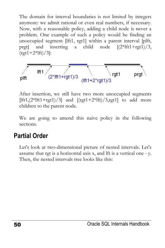
The domain for interval boundaries is not limited by integers anymore: we admit rational or even real numbers, if necessary. Now, with a reasonable policy, adding a child node is never a problem. One example of such a policy would be finding an unoccupied segment [lft1, rgt1] within a parent interval [plft, prgt] and inserting a child node [(2*lft1+rgt1)/3, (rgt1+2*lft)/3]:

After insertion, we still have two more unoccupied segments [lft1,(2*lft1+rgt1)/3] and [(rgt1+2*lft)/3,rgt1] to add more children to the parent node. We are going to amend this naive policy in the following sections.

Partial Order Let's look at two-dimensional picture of nested intervals. Let's assume that rgt is a horizontal axis x, and lft is a vertical one - y. Then, the nested intervals tree looks like this:


Each node [lft, rgt] has its descendants bounded within the two-dimensional cone y >= lft & x <= rgt. Since the right interval boundary is always less than the left one, none of the nodes are allowed above the diagonal y = x. The other way to look at this picture is to notice that a child node is a descendant of the parent node whenever a set of all points defined by the child cone y >= clft & x <= crgt is a subset of the parent cone y >= plft & x <= prgt. A subset relationship between the cones on the plane is a partial order.

Partial Order 51

Now that we know the two constraints to which tree nodes conform, I'll describe exactly how to place them at the xy plane.

The Mapping Tree root choice is completely arbitrary: we'll assume the interval [0,1] to be the root node. In our geometrical interpretation, all the tree nodes belong to the lower triangle of the unit square at the xy plane. We'll describe further details of the mapping by induction. For each node of the tree, let's first define two important points at the xy plane. The depth-first convergence point is an intersection between the diagonal and the vertical line through the node. For example, the depth-first convergence point for <x=1,y=1/2> is <x=1,y=1>. The breadth-first convergence point is an intersection between the diagonal and the horizontal line through the point. For example, the breadth-first convergence point for <x=1,y=1/2> is <x=1/2,y=1/2>. Now, for each parent node, we define the position of the first child as a midpoint halfway between the parent point and depth-first convergence point. Then, each sibling is defined as a midpoint halfway between the previous sibling point and breadth-first convergence point:


For example, node 2.1 is positioned at x=1/2, y=3/8. Now that the mapping is defined, it is clear which dense domain we are using: it's not rationals, and not reals either, but binary fractions (although, the former two would suffice, of course). Interestingly, the descendant subtree for the parent node "1.2" is a scaled down replica of the subtree at node "1.1." Similarly, a subtree at node 1.1 is a scaled down replica of the tree at node "1." A structure with self-similarities is called a fractal.

The Mapping 53

Normalization Next, we notice that x and y are not completely independent. We can tell what are both x and y if we know their sum. Given the numerator and denominator of the rational number representing the sum of the node coordinates, we can calculate x and y coordinates back as: function x_numer( numer integer, denom integer ) RETURN integer IS ret_num integer; ret_den integer; BEGIN ret_num := numer+1; ret_den := denom*2; while floor(ret_num/2) = ret_num/2 loop ret_num := ret_num/2; ret_den := ret_den/2; end loop; RETURN ret_num; END; function x_denom( numer integer, denom integer ) ... RETURN ret_den; END;

in which function x_denom body differs from x_numer in the return variable only. Informally, numer+1 increment would move the ret_num/ret_den point vertically up to the diagonal, and then x coordinate is half of the value, so we just multiplied the denominator by two. Next, we reduce both numerator and denominator by the common power of two. Naturally, y coordinate is defined as a complement to the sum:


function y_numer( numer integer, denom integer ) RETURN integer IS num integer; den integer; BEGIN num := x_numer(numer, denom); den := x_denom(numer, denom); while den < denom loop num := num*2; den := den*2; end loop; num := numer - num; while floor(num/2) = num/2 loop num := num/2; den := den/2; end loop; RETURN num; END; function y_denom( numer integer, denom integer ) ... RETURN den; END;

Now, the test (where 39/32 is the node 1.3.1): select x_numer(39,32)||'/'||x_denom(39,32), y_numer(39,32)||'/'||y_denom(39,32) from dual 5/8 19/32 select 5/8+19/32, 39/32 from dual 1.21875 1.21875

I don't use a floating point to represent rational numbers, and wrote all the functions with integer arithmetic instead. To put it bluntly, the floating point number concept in general, and the IEEE standard in particular, is useful for rendering 3D-game graphics only. In the last test, however, we used a floating point just to verify that 5/8 and 19/32, returned by the previous query, do indeed add to 39/32.

Normalization 55

We'll store two integer numbers — numerator and denominator of the sum of the coordinates x and y — as an encoded node path. Incidentally, Celko's nested sets use two integers as well. Unlike nested sets, our mapping is stable: each node has a predefined placement at the xy plane, so that the queries involving node position in the hierarchy could be answered

without reference to the database. In this respect, our hierarchy model is essentially a materialized path encoded as a rational number.

Finding Parent Encoding and Sibling Number Given a child node with numer/denom encoding, we find the node's parent like this: function parent_numer( numer integer, denom integer ) RETURN integer IS ret_num integer; ret_den integer; BEGIN if numer=3 then return NULL; end if; ret_num := (numer-1)/2; ret_den := denom/2; while floor((ret_num-1)/4) = (ret_num-1)/4 loop ret_num := (ret_num+1)/2; ret_den := ret_den/2; end loop; RETURN ret_num; END; function parent_denom( numer integer, denom integer ) ... RETURN ret_den; END;

The idea behind the algorithm is the following: If the node is on the very top level — and all these nodes have a numerator equal to 3 — then the node has no parent. Otherwise, we must move vertically down the xy plane at a distance equal to the distance from the depth-first convergence point. If the node happens to be the first child, then that is the answer. Otherwise, we must move horizontally at a distance equal to the distance from the breadth-first convergence point until we meet the parent node. Here is the test of the method (in which 27/32 is the node 2.1.2, while 7/8 is 2.1):


select parent_numer(27,32)||'/'||parent_denom(27,32) from dual 7/8

In the previous method, counting the steps when navigating horizontally would give the sibling number: function sibling_number( numer integer, denom integer ) RETURN integer IS ret_num integer; ret_den integer; ret integer; BEGIN if numer=3 then return NULL; end if; ret_num := (numer-1)/2; ret_den := denom/2; ret := 1; while floor((ret_num-1)/4) = (ret_num-1)/4 loop if ret_num=1 and ret_den=1 then return ret; end if; ret_num := (ret_num+1)/2; ret_den := ret_den/2; ret := ret+1; end loop; RETURN ret; END;

For a node at the very first level a special stop condition, ret_num=1 and ret_den=1 is needed. The test: select sibling_number(7,8) from dual 1

Calculating Materialized Path and Distance between nodes

Strictly speaking, we don't have to use a materialized path, since our encoding is an alternative. On the other hand, a materialized path provides a much more intuitive visualization of the node position in the hierarchy, so that we can use the

Calculating Materialized Path and Distance between nodes 57

materialized path for input and output of the data if we provide the mapping to our model. Implementation is a simple application of the methods from the previous section. We print the sibling number, jump to the parent, then repeat the above two steps until we reach the root: function path( numer integer, denom integer ) RETURN varchar2 IS BEGIN if numer is NULL then return ''; end if; RETURN path(parent_numer(numer, denom), parent_denom(numer, denom)) || '.' || sibling_number(numer, denom); END; select path(15,16) from dual .2.1.1

Now we are ready to write the main query: given the 2 nodes, P and C, when P is the parent of C? A more general query would return the number of levels between P and C if C is reachable from P, and some exception indicator; otherwise: function distance( num1 integer, den1 integer, num2 integer, den2 integer ) RETURN integer IS BEGIN if num1 is NULL then return -999999; end if; if num1=num2 and den1=den2 then return 0; end if; RETURN 1+distance(parent_numer(num1, den1), parent_denom(num1, den1), num2,den2); END; select distance(27,32,3,4) from dual 2

Negative numbers are interpreted as exceptions. If the num1/den1 node is not reachable from num2/den2, then the navigation converges to the root, and level(num1/den1)-


999999 would be returned (readers are advised to find a less clumsy solution). The alternative way to answer whether two nodes are connected is by simply calculating the x and y coordinates, and checking if the parent interval encloses the child. Although none of the methods refer to disk, checking whether the partial order exists between the points seems much less expensive! On the other hand, it is just a computer architecture artifact that comparing two integers is an atomic operation. More thorough implementation of the method would involve a domain of integers with a unlimited range (those kinds of numbers are supported by computer algebra systems), so that a comparison operation would be iterative as well. Our system wouldn't be complete without a function inverse to the path, which returns a node's numer/denom value once the path is provided. Let's introduce two auxiliary functions, first: function child_numer ( num integer, den integer, child integer ) RETURN integer IS BEGIN RETURN num*power(2, child)+3-power(2, child); END; function child_denom ( num integer, den integer, child integer ) RETURN integer IS BEGIN RETURN den*power(2, child); END; select child_numer(3,2,3) || '/' || child_denom(3,2,3) from dual 19/16

For example, the third child of the node 1 (encoded as 3/2) is the node 1.3 (encoded as 19/16).

Calculating Materialized Path and Distance between nodes 59

The path encoding function is: function path_numer( path varchar2 ) RETURN integer IS num integer; den integer; postfix varchar2(1000); sibling varchar2(100); BEGIN num := 1; den := 1; postfix := '.' || path || '.'; while length(postfix) > 1 loop sibling := substr(postfix, 2, instr(postfix,'.',2)-2); postfix := substr(postfix, instr(postfix,'.',2), length(postfix) -instr(postfix,'.',2)+1); num := child_numer(num,den,to_number(sibling)); den := child_denom(num,den,to_number(sibling)); end loop; RETURN num; END; function path_denom( path varchar2 ) ... RETURN den; END; select path_numer('2.1.3') || '/' || path_denom('2.1.3') from dual 51/64

The Final Test Now that the infrastructure is completed, we can test it. Let's create the hierarchy create table emps ( name varchar2(30), numer integer, denom integer ) alter table emps ADD CONSTRAINT uk_name UNIQUE (name) USING INDEX (CREATE UNIQUE INDEX name_idx on emps(name)) ADD CONSTRAINT UK_node UNIQUE (numer, denom) USING INDEX (CREATE UNIQUE INDEX node_idx on emps(numer, denom))


and fill it with some data: insert into emps values ('KING', path_numer('1'),path_denom('1')); insert into emps values ('JONES', path_numer('1.1'),path_denom('1.1')); insert into emps values ('SCOTT', path_numer('1.1.1'),path_denom('1.1.1')); insert into emps values ('ADAMS', path_numer('1.1.1.1'),path_denom('1.1.1.1')); insert into emps values ('FORD', path_numer('1.1.2'),path_denom('1.1.2')); insert into emps values ('SMITH', path_numer('1.1.2.1'),path_denom('1.1.2.1')); insert into emps values ('BLAKE', path_numer('1.2'),path_denom('1.2')); insert into emps values ('ALLEN', path_numer('1.2.1'),path_denom('1.2.1')); insert into emps values ('WARD', path_numer('1.2.2'),path_denom('1.2.2')); insert into emps values ('MARTIN', path_numer('1.2.3'),path_denom('1.2.3')); insert into emps values ('TURNER', path_numer('1.2.4'),path_denom('1.2.4')); insert into emps values ('CLARK', path_numer('1.3'),path_denom('1.3')); insert into emps values ('MILLER', path_numer('1.3.1'),path_denom('1.3.1')); commit;

All the functions written in the previous sections are conveniently combined in a single view: create or replace view hierarchy as select name, numer, denom, y_numer(numer,denom) numer_left, y_denom(numer,denom) denom_left, x_numer(numer,denom) numer_right, x_denom(numer,denom) denom_right, path (numer,denom) path, distance(numer,denom,3,2) depth from emps

And, finally, we can create the hierarchical reports. Depth-first enumeration, ordering by left interval boundary

The Final Test 61

select lpad(' ',3*depth)||name from hierarchy order by numer_left/denom_left LPAD('',3*DEPTH)||NAME ----------------------------------------------- KING CLARK MILLER BLAKE TURNER MARTIN WARD ALLEN JONES FORD SMITH SCOTT ADAMS

Depth-first enumeration, ordering by right interval boundary select lpad(' ',3*depth)||name from hierarchy order by numer_right/denom_right desc LPAD('',3*DEPTH)||NAME ----------------------------------------------------- KING JONES SCOTT ADAMS FORD SMITH BLAKE ALLEN WARD MARTIN TURNER CLARK MILLER

Depth-first enumeration, ordering by path (output identical to #2)


select lpad(' ',3*depth)||name from hierarchy order by path LPAD('',3*DEPTH)||NAME ----------------------------------------------------- KING JONES SCOTT ADAMS FORD SMITH BLAKE ALLEN WARD MARTIN TURNER CLARK MILLER

All the descendants of JONES, excluding himself: select h1.name from hierarchy h1, hierarchy h2 where h2.name = 'JONES' and distance(h1.numer, h1.denom, h2.numer, h2.denom)>0; NAME ------------------------------ SCOTT ADAMS FORD SMITH

All the ancestors of FORD, excluding himself: select h2.name from hierarchy h1, hierarchy h2 where h1.name = 'FORD' and distance(h1.numer, h1.denom, h2.numer, h2.denom)>0; NAME ------------------------------ KING JONES

The Final Test 63

SQL Tuning Improvements

CHAPTER

6 SQL Tuning Improvements in Oracle 9.2

Tuning a single SQL query is an enormously important topic. Before going into production virtually every system would expose some statements that require tuning. In this article, we'll explore several Oracle 9.2 improvements that make life of performance analyst easier.

Access and Filter Predicates Syntactically, SQL query consists of three fundamental parts: a list of columns, a list of tables, and a "where" clause.

The "where" clause is a logical formula that can be further decomposed into predicates connected by Boolean connectives. For example, the "where" clause of: select empno, sal from emp e, dept d where e.deptno = d.deptno and dname = 'ACCOUNTING'

Is a conjunction of dname = 'ACCOUNTING' single table predicate and e.deptno = d.deptno join predicate. Arguably, predicate handling is the heart of SQL optimization: predicates could be transitively added, rewritten using Boolean Algebra laws, moved around at SQL Execution Plan, and so on. In our simplistic example, the single table predicate is


applied either to index or table scan plan nodes, while join predicate could also be applied to the join node. Unfortunately, despite their significance, Oracle Execution Plan facility didn't show predicates until version 9.2. (although experts had an option of running 10060 event trace). In the latest release plan_table (together with its runtime sibling v$sql_plan) acquired two new columns: ACCESS_PREDICATES VARCHAR(4000) FILTER_PREDICATES VARCHAR(4000)

In our example, the plan

OPERATION OPTIONS OBJECT NAME

FILTER PREDICATES

SELECT STATEMENT

NESTED LOOPS TABLE ACCESS FULL DEPT D.DNAME= ACCOUNTING' TABLE ACCESS FULL EMP E.DEPTNO= .DEPTNO now explicitly shows us that dname = 'ACCOUNTING' single table predicate is filtering rows during the outer table scan, while e.deptno = d.deptno join predicate is applied during each inner table scan. I found it convenient to apply a little bit of GUI "sugarcoating" and display the plan as

Access and Filter Predicates 65

OPERATION OPTIONS OBJECT NAME SELECT STATEMENT

NESTED LOOPS TABLE ACCESS FULL DEPT

Filter Predicates D.DNAME=’ACCOUNTING’

TABLE ACCESS FULL EMP Filter Predicates

E.DEPTNO=D.DEPTNO especially in the cases where predicates are complex. Consider an example with nested subquery: select empno, sal from emp e where sal in (select max(sal) from emp ee)



E.SAL= (SELECT /*+ */ MAX(EE.SAL) FROM EMP EE) SORT AGGREGATE

TABLE ACCESS FULL EMP Here the filter predicate contains the whole subquery! Again, predicate visualization helps understanding how the plan is executed. Since the subquery is not correlated, it can be evaluated once only. Two innermost plan nodes are responsible for execution of nested subquery. Then, the emp e table from the outer query block is scanned, and only the rows that meet filter condition remain in the result set. My next example demonstrates predicate transitivity: select e.empno, d.dname from emp e, dept d where e.deptno = d.deptno and e.deptno = 10



MERGE JOIN CARTESIAN INDEX RANGE SCAN IND_DNO_DNAME

Access Predicates D.DEPTNO=10

BUFFER SORT TABLE ACCESS FULL EMP

Filter Predicates E.DEPTNO=10

From the plan, it becomes obvious that the optimizer chose a Cartesian Product because it considered worthwhile dropping join predicate e.deptno = d.deptno and using the derived d.deptno = 10 predicate instead. In this example, we also see the Access Predicates in action for the first time. If we add one more predicate select e.empno, d.dname from emp e, dept d where e.deptno = d.deptno and e.deptno = 10 and dname like '%SEARCH'


MERGE JOIN CARTESIAN INDEX RANGE SCAN IND_DNO_DNAME

Access Predicates AND

D.DEPTNO=10 D.DNAME LIKE ‘%SEARCH’

Filter Predicates D.DNAME LIKE ‘%SEARCH’

BUFFER SORT TABLE ACCESS FULL EMP

Filter Predicates E.DEPTNO=10

Access and Filter Predicates 67

then we see that both Filter and Access predicates can be applied at the same node. Naturally, only d.deptno = 10 conjunct can be used as a start and stop key condition for the index range scan. The dname like '%SEARCH' predicate is then applied as a filter. Predicates allow us to see artifacts hidden deep under the sql engine hood. For example, consider the following query: select ename from emp where ename like 'MIL%'



AND EMP.ENAME LIKE ‘%MIL%’ UPPER(EMP.ENAME) LIKE ‘%MIL%’

When I saw this plan my natural question was, where did the second conjunct UPPER(ename) like UPPER('MIL%') came from? After a quick investigation, I found that there was a check constraint UPPER(ename) = ename declared upon the emp table. In other words, Oracle leverages check constraints when manipulating query predicates! If we add a function-based index upon UPPER(ename) pseudocolumn, then it would be used, even though the original query doesn't have any function calls within the predicate: select ename from emp where ename like 'MIL%'



TABLE ACCESS BY INDEX ROWID EMP

Filter Prediates EMP.ENAME LIKE ‘MIL%’

INDEX RANGE SCAN IND_UPPER_ENAME Access Predicates

UPPER(EMP.ENAME) LIKE ‘MIL%’ Filter Predicates

UPPER(EMP.ENAME) LIKE ‘MIL%’

V$SQL_PLAN_STATISTICS There is a well-known Achilles' heel in SQL optimization: the cost-based plan is as reliable as the cost estimation is. Several factors contribute to inherent difficulty of realistic cost estimation: 1. Complex predicates. Complex predicate expressions

include either multiple predicates connected with Boolean connectives, or user-defined functions, domain operators, and subqueries in the individual predicates, or any combination of the above. For example, when estimating selectivity of power(10,sal) + sal > 2000 and sal > 1000 predicate, the first problem we face is estimating selectivity of the power(10,sal) + sal > 2000 conjunct alone. The second problem is an obvious correlation between both conjuncts. In some cases dynamic sampling comes to the rescue, while in the worst case a user would be at the mercy of heuristic - default selectivity.

2. Bind variables. Parse time and execution time in this case are the two conflicting goals. Bind variables were designed to amortize parse time overhead among multiple query executions. It negatively affected the quality of the plans,

V$SQL_PLAN_STATISTICS 69

however, since much less can be inferred about selectivity of a predicate with a bind variable.

3. Data Caching. With caching a simplistic model where the cost is based upon the number of logical I/Os is no longer valid: cost model adjustment and caching statistics is necessary.

New dictionary view v$sql_plan_statistics and its sibling v$sql_plan_statistics_all (joining the former with v$sql_plan) were introduced in order to help performance analyst to quicker recognize query optimization problems. In my experience, the following two columns are indispensable: LAST_CR_BUFFER_GETS NUMBER LAST_OUTPUT_ROWS NUMBER

When evaluating the quality of the plan, I measure up the COST against last_cr_buffer_gets, and CARDINALITY against last_output_rows. Before v$sql_plan_statistics was introduced it was still possible to know the number of row processed at each plan node (or speaking more accurately - row source) from TKPROF output, of course. It also was possible to get cumulative I/O and other statistics for each SQL statement. Statistics table, however, gives itemized report per each plan node, and is, therefore, both more detailed and more convenient. Let's jump to the examples. Our first exercise is fairly trivial: scanning the full table that was not analyzed: alter session set OPTIMIZER_DYNAMIC_SAMPLING = 0; select /*+all_rows*/ * from small;


OPERATION OPTIONS OBJECT NAME CARD LAST OUTPUT ROWS

TABLE ACCESS FULL SMALL 607200 30000 Here, I set optimizer_dynamic_sampling = 0 because the default setting in Oracle release 2 has been increased to 1, and the hint is used to force CBO mode. The discrepancy between the number of row processed and the estimated cardinality is because there is no statistics on the table. Let's raise sampling level in our experiment: alter session set OPTIMIZER_DYNAMIC_SAMPLING = 2; select /*+all_rows*/ * from small;

OPERATION OPTIONS OBJECT NAME CARD LAST OUTPUT ROWS

TABLE ACCESS FULL SMALL 33871 30000 Now, estimation discrepancy is negligible. (Sampling levels are documented at: http://otn.oracle.com/docs/products/oracle9i/doc_library/ release2/server.920/a96533/hintsref.htm#11792.) In our final example, lets explore classic Indexed Nested Loops: select s1.id,s2.id from small s1, small s2 where s1.id =1 and s1.data=s2.data

V$SQL_PLAN_STATISTICS 71

OPERATION OPTIONS OBJECT NAME

LAST OUTPUT ROWS

LAST CR BUFFER

GETS NESTED LOOPS 1 8

TABLE ACCESS BY INDEX ROWID SMALL 1 4

INDEX UNIQUE SCAN SMALL_PK 1 3 Access Predicates

ID=1

TABLE ACCESS BY INDEX ROWID SMALL 1 4

INDEX RANGE SCAN SMALL_ DATA_KEY 1 3

Access Predicates DATA=DATA

I deliberately made up the example so that each plan node processes one row only. In that case, the execution statistics are quite pronounced. The example starts with a unique index scan of the primary key. Since we have 30000 rows total, then the B-Tree index has three levels, and, therefore, we see exactly three logical I/Os at the plan statistics node. Next, the execution dereferences a pointer from B-Tree leaf to the table row. It's just one more block read. After the row from the driving table is known, the inner block of the Nested Loop can be executed; specifically, index range scan is performed first. Since the result of the range scan is a single B-Tree leaf, the statistics is identical to that of the unique index scan in the outer branch. We therefore have four more block reads. And, finally, the overall execution I/O is just a sum 4+4=8 of both inner and outer Nested Loops plan branches. My thanks to the Benoit Dageville and Mohamed Zait who implemented those features. I'm also grateful to my colleague Vladimir Barriere whose comments improved the article.


Oracle SQL Tuning Tips CHAPTER

7 SQL tuning

Oracle SQL tuning is a phenomenally complex subject, and entire books have been devoted to the nuances of Oracle SQL tuning. However there are some general guidelines that every Oracle DBA follows in order to improve the performance of their systems. The goals of SQL tuning are simple: Remove unnecessary large-table full table scans

Unnecessary full table scans cause a huge amount of unnecessary I/O, and can drag down an entire database. The tuning expert first evaluates the SQL based on the number of rows returned by the query. If the query returns less and 40 percent of the table rows in an ordered table, or 7 percent of the rows in an unordered table), the query can be tuned to use an index in lieu of the full table scan. The most common tuning for unnecessary full table scans is adding indexes. Standard B-tree indexes can be added to tables, and bitmapped and function-based indexes can also eliminate full table scans. The decision about removing a full table scan should be based on a careful examination of the I/O costs of the index scan vs. the costs of the full table scan, factoring in the multiblock reads and possible parallel execution. In some cases an unnecessary full table scan can be forced to use an index by adding an index hint to the SQL statement. Cache small-table full table scans In cases where a full table

scan is the fastest access method, the tuning professional should ensure that a dedicated data buffer is available for the rows. In Oracle7 you can issue alter table xxx cache. In

SQL tuning 73

Oracle8 and beyond, the small table can be cached by forcing to into the KEEP pool. Verify optimal index usage This is especially important for

improving the speed of queries. Oracle sometimes has a choice of indexes, and the tuning professional must examine each index and ensure that Oracle is using the proper index. This also includes the use of bitmapped and function-based indexes. Verify optimal JOIN techniques Some queries will perform

faster with NESTED LOOP joins, others with HASH joins, while other favor sort-merge joins.

These goals may seem deceptively simple, but these tasks comprise 90 percent of SQL tuning, and they don't require a through understanding of the internals of Oracle SQL. Let's begin with an overview of the Oracle SQL optimizers.


Altering SQL Stored Outlines

CHAPTER

8 Faking Stored Outlines in Oracle 9

In a previous article, I discussed stored outlines and described one mechanism for abusing the system to produce the stored outline that you needed to have. I also pointed out that there was some risk in using this method with Oracle 9, as the details stored in the database had become much more complex. In this follow-up article, I present a legal way of manipulating a stored outline that can be applied both in Oracle 8 and in Oracle 9. Details in this article were based on experiments carried out on default installations of Oracle 8.1.7.0 and Oracle 9.2.0.1.

Review What are you supposed to do when you know how to make a piece of DML run much more quickly by adding a few hints, but don't have access to the source code to put those hints in the right place? In the last article I showed how you might be able to take advantage of stored outlines (also known as plan stability) to get the database engine to do the job for you. A stored outline consists (loosely speaking) of two components - an SQL statement that you wish to control, and a list of hints that Oracle should apply to that SQL statement whenever it sees it being optimized. Both components are stored in the database in a schema called outln.

Faking Stored Outlines in Oracle 9 75

We can check the list of stored SQL statements, and the hints that will be attached to them, using a couple of queries like those in figure 1. select name, used, sql_text from user_outlines where category = 'DEFAULT' ; select stage, node, hint from user_outline_hints where name = '{one of the names}' ;

Figure 1: Examining stored outlines.

In the previous article, I introduced the idea of deceiving the system by creating a stored outline using legal methods, and then patching the outln tables by using a couple of SQL statements to swap the actual result for a stored outline you had created for a similar, but hinted, statement. At the time I mentioned that this was probably safe for Oracle 8, but could lead to problems in Oracle 9 because of changes made in the newer version. This article examines those changes, and introduces a legal way of getting your preferred set of hints registered in the outln tables against your problem queries.

The Changes If you connect to the outln schema (which is locked by default in Oracle 9) and list the available tables, you will find that Oracle 9 has one more table than Oracle 8. The tables are:


ol$ The sql ol$hints The hints

ol$notes The query blocks The third table is the new table, and is used to associate the list of hints with different blocks in the (internally rewritten version of the) SQL query. You will also find that the list of hints (ol$hints) has been enhanced with details of text lengths and offsets. Descriptions of all three tables appear in figure 2, with the new columns for Oracle 9 marked by stars. Ol$ OL_NAME VARCHAR2(30) SQL_TEXT LONG TEXTLEN NUMBER SIGNATURE RAW(16) HASH_VALUE NUMBER HASH_VALUE2 NUMBER *** CATEGORY VARCHAR2(30) VERSION VARCHAR2(64) CREATOR VARCHAR2(30) TIMESTAMP DATE FLAGS NUMBER HINTCOUNT NUMBER SPARE1 NUMBER *** SPARE2 VARCHAR2(1000) *** Ol$hints OL_NAME VARCHAR2(30) HINT# NUMBER CATEGORY VARCHAR2(30) HINT_TYPE NUMBER HINT_TEXT VARCHAR2(512) STAGE# NUMBER NODE# NUMBER TABLE_NAME VARCHAR2(30) TABLE_TIN NUMBER TABLE_POS NUMBER REF_ID NUMBER *** USER_TABLE_NAME VARCHAR2(64) *** COST FLOAT(126) *** CARDINALITY FLOAT(126) *** BYTES FLOAT(126) *** HINT_TEXTOFF NUMBER *** HINT_TEXTLEN NUMBER ***

The Changes 77

JOIN_PRED VARCHAR2(2000) *** SPARE1 NUMBER *** SPARE2 NUMBER *** ol$nodes (completely new in 9) OL_NAME VARCHAR2(30) CATEGORY VARCHAR2(30) NODE_ID NUMBER PARENT_ID NUMBER NODE_TYPE NUMBER NODE_TEXTLEN NUMBER NODE_TEXTOFF NUMBER

Figure 2: The outln tables. A couple of details you might notice immediately -- the views defined on top of these tables clearly exclude a lot of useful information. Despite the ten extra columns in ol$hints the view definition for user_outline_hints has not changed. In fact, this view was sadly deficient in Oracle 8, omitting, as it did, the rather informative hint#. You will also notice that Oracle 9 now has two hash_value columns. If you build identical statements in an Oracle 8 and an Oracle 9 database, you will find that they match on their hash_value, but the Oracle 9 hash_value2 is probably completely different. You will also find that the signature in Oracle 9 is different from its value in Oracle 8. This is because of a major change in strategy between the two versions aimed at increasing the re-use of stored outlines. Under Oracle 8 you could only use a stored outline if your SQL matched the stored SQL exactly - to the last space, capital, and line-feed. Under Oracle 9, the rules are relaxed, so that a statement is matched after repetitive "white space" is eliminated and the text has been folded to the same case. For example, the following two statements will use the same outline.


select * from t1 where id = 5; SELECT * FROM T1 WHERE ID = 5;

This change in strategy results in a change in the signature for the SQL that first generates the plan; and if you upgrade from Oracle 8 to Oracle 9, you will have to regenerate stored outlines or you may find that they don't appear to work any more. (In fact, the package outln_pkg, aliased to dbms_outln, includes a special procedure update_signatures to handle this problem). The most significant thing about the version 9 tables, however, is the extreme level of detail about the text and objects involved in the query. Create the example shown in figure 3, and take a look at the content of the ol$hints table before reading on. drop table t1; create table t1 nologging as select rownum id, rownum n1, object_name, rpad('x',500) padding from all_objects where rownum <= 100 ;

The Changes 79

alter table t1 add constraint t1_pk primary key (id); create index t1_i1 on t1(n1); analyze table t1 compute statistics; create or replace outline demo_1 on select * from t1 where id = 5 and n1 = 10 ;

Figure 3: Sample code. The example is based on a small, simple table, with two identical columns, one defined (and therefore indexed) as a primary key, one with a simple, non-unique index. We generate a stored outline for a typical query and then see what we can do with it. If we run our sample queries from figure 1 against the demo_1 plan, generated by this example, we find the following six hints attached to the query: STAGE NODE HINT 3 1 NO_EXPAND 3 1 ORDERED 3 1 NO_FACT(T1) 3 1 INDEX(T1 T1_PK) 2 1 NOREWRITE 1 1 NOREWRITE

As expected, the fourth line shows us that we have used the primary key index (T1_Pk) to access the table. But what could we do about the stored outline if we really wanted Oracle to use the non-unique index T1_I1? Ideally we would like to tweak this stored outline so that the line reading 3 1 INDEX(T1 T1_PK) became 3 1 INDEX(T1 T1_I1)


New Features The first thing we could do is look at the package dbms_outln_edit. This appeared in Oracle 9 and, as its name suggests, it is a package aimed at editing stored outlines, so this looks promising. However, describing the package, and checking the manuals, we note that the package contains only the following 'edit-related' procedures: CREATE_EDIT_TABLES DROP_EDIT_TABLES CHANGE_JOIN_POS

The first two procedures allow us to create and drop local copies of the tables normally owned by outln. The third allows us to swap the order of table joins in a stored plan. There is nothing that lets us simply modify a single hint. At present, the package seems to be virtually useless -- but it's bound to become more sophisticated. Plan B, of course, is to hack! If we connect as outln, and examine the contents of the ol$hints table (which underpins the user_outline_hints view) we could try the following update: update ol$hints set hint_text = 'INDEX(T1 T1_I1)' where ol_name = 'demo_1' and hint# = 4 ;

Connecting back to our test schema, flushing the shared pool, and switching on stored outlines:

New Features 81

connect test_user/test alter system flush shared_pool; alter session set use_stored_outline=true;

we find that the hacked plan does, indeed, work as required. But it's not a comfortable solution given the strict warnings we are usually given about 'updating the data dictionary'.

Old Methods (1) Our aim, then, is to find a devious, but seemingly innocent method of changing the content of the outline tables without hacking them directly. Historically (before version 9) we could achieve this in a couple of ways, based on the fact that the effect of an outline was dictated purely by the text of the incoming SQL statement, and not by any consideration of object type or ownership. One option (originally described, I believe, by Tom Kyte in his book Expert One on One: Oracle) works by replacing tables with hinted views. Connect to another schema that has access to the T1 table and create a hinted view of the same name with the following definition: Create or replace view t1 as Select /*+ index(t1,t1_i1) */ * from test_user.t1;

Once this view is in place, use this schema to 'recompile' the existing outline with the command: alter outline demo_1 rebuild;


Note - you need the privilege alter any outline to be able to execute this command. If we go back to the original schema, flush the shared pool, and switch on stored outlines, we find that our original query now uses the T1_I1 index as required. Why does this work? Because stored outlines do not belong to a schema. When we rebuilt the outline called demo_1 from the new schema, the name T1 applied to a local view which contained a hint, so Oracle folded the hint into the actual execution plan, and therefore into the outline. Looking at the view user_outline_hints view, we find that the critical line has indeed become 3 1 INDEX(T1 T1_I1)

Unfortunately, we will also note that there are now three lines of the form: 2 1 NOREWRITE 1 2 NOREWRITE 1 1 NOREWRITE

Originally we had only the two lines: 2 1 NOREWRITE 1 1 NOREWRITE

We have introduced a hint that applies to 'Stage 1, Node 2'. I don't claim to know exactly what this means, but it must relate to the fact that in parsing and optimizing the query from the other schema, Oracle has performed an extra step of converting a view reference to a base table reference.

Old Methods (1) 83

Although, at present, this does not stop the outline from being applied correctly (or so it seems in this simple case) who can say how fussy Oracle might become in future releases.

Old Methods (2) Because views introduce an anomaly that might turn into an error in a future release, we have to be fussier. So let's try the following: Create a new schema. Create table T1 in that schema. Create ONLY the index T1_I1. Rebuild the outline in that schema

If we compare the contents of view user_outline_hints for our outline before and after the rebuild (we have to recconect to the original schema to do so), we will find that they are identical apart from the one line that we wanted to alter. Connecting back to our original schema and doing the usual check of flushing the shared pool and switching on outlines, we find that the modified outline is used. However there is a hidden threat, this time a little more subtle. Go back to figure 2 with its definitions of the new columns that appear in Oracle 9 - what information do you think is kept in the column user_table_name? It is the qualified table name; i.e., {User_name}.{table_name}

In our example this will tell Oracle that table T1 is actually a table belonging to the new schema, not to the original schema. Even though Oracle is using the stored outline, the information in the table is sufficient to tell it that it is applying the plan to the wrong object.


Again, it works at present, but why is the information there -- possibly because of enhancements coming in future releases.

The Safe Bet It seems that there is only one way to generate a stored outline which doesn't expose you to future risk -- be as honest as possible. Do it in the right schema with the right objects. In this case, you need to drop the primary key index, generate the plan, and then replace the primary key! Of course you might not want to do this on a production system, and even if you did it is possible that the outline would switch to a full tablescan. The bottom line is that you need to have at least one spare copy of the schema (i.e. with the same name) on another database, and then you need to manipulate that copy very carefully to get the outline you need. Once you have the outline, you can export from one database and import it to the other. For example: on the spare database, it would be okay to drop the primary key to avoid the PK unique scan. If Oracle didn't then take the other index automatically, you can tell all sorts of lies, such as: Change the optimizer_mode to first_rows_1. Create data that is unique across column N1. (Don't make it

a unique index, though, or the generated outline will be a unique scan instead of a range scan). Use dbms_stats to say that the index has a fantastic

clustering_factor. The Safe Bet 85

Use optimizer_index_caching to say that the index is 100% cached. Use optimizer_index_cost_adj to say that a multiblock read is

100 times as slow as a single block read. Use dbms_stats to make the same claim through aux_stats$,

and add in the fact that the typical size of a multiblock read is two blocks. Rebuild the index to include both the columns in the where

clause. Given the current content of the outline tables, almost anything goes provided that table owners don't change, object types don't change, and indexes don't change their uniqueness. If you can construct a data set and environment that produces an outline that has no internal inconsistencies on the production system, then you can cheat in almost any way you like.

Conclusion The information that goes into a Stored Outline in Oracle 9 is much subtler than it was in Oracle 8. It used to be quite easy and apparently risk-free to 'adjust' outlines. The methods still work, but the huge volume of extra information collected in Oracle 9 tends to suggest that earlier methods now carry a future risk. Although Oracle 9 has introduced a package to edit stored outlines, it is currently limited to swapping table orders. Short of using a second system with changed indexes, an altered environment and contrived statistics, it no longer seems safe to tamper with stored outlines.


References Oracle 9i Release 2: Database Performance Tuning Guide and Reference -- Chapter 7. Oracle 9I Release 2: Supplied PL/SQL Packages and Types Reference -- Chapters 41 - 42.

References 87

Using Bitmap Indexes with Oracle

CHAPTER

9 Understanding Bitmap Indexes

Bitmap indexes are a great boon to certain kinds of application, but there is a lot of mis-information in the field about how they work, when to use them, and the side-effects. This article examines the structure of bitmap indexes, and tries to explain how some of the more commonly repeated misconceptions came into existence.

Everybody Knows … If you did a quick survey to discover the understanding that people had of bitmap indexes, you would probably find the following comments being quoted fairly frequently: When there are bitmap indexes on tables then updates will

take out full table locks. Bitmap indexes are good for low-cardinality columns. Bitmap index scans are more efficient than tablescans even

when returning a large fraction of a table. The third claim is really little more than a (possibly untested) corollary to the second claim. And all three claims are in that grey area somewhere between false and extremely misleading. Of course, there is a faint element of truth to these claims -- just enough to explain why they should have arisen in the first place.


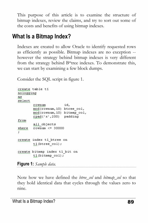
This purpose of this article is to examine the structure of bitmap indexes, review the claims, and try to sort out some of the costs and benefits of using bitmap indexes.

What Is a Bitmap Index? Indexes are created to allow Oracle to identify requested rows as efficiently as possible. Bitmap indexes are no exception -- however the strategy behind bitmap indexes is very different from the strategy behind B*tree indexes. To demonstrate this, we can start by examining a few block dumps. Consider the SQL script in figure 1.

Figure 1: Sample data.

Note how we have defined the btree_col and bitmap_col so that they hold identical data that cycles through the values zero to nine.

What Is a Bitmap Index? 89

On a 9.2 database with a block size of 8K, the resulting table was 882 blocks long. The B*tree index had 57 leaf blocks, and the bitmap index had 10 leaf blocks.

Figure 2: Symbolic block dumps.

Clearly the bitmap index was in some way much more tightly packed than the B*tree index. To see the packing, we can produce a symbolic dump from the indexes using commands like: alter system dump datafile x block y;

See figure 2 for results -- be warned, however, that symbolic block dumps can be a little misleading. Some of the information they display is derived, some is re-arranged for the sake of clarity.


Do Bitmaps Lock Tables? Looking at figure 2, we see in the B*tree index that every entry consists of a set of flags, a lock byte, and (in this case) two columns of data. The two columns are in fact the indexed value, and a rowid -- and every row in our table has a corresponding entry of this form in the index. (If the index were a unique index, we would still see the same content in each entry, but the layout would be a little different). In the bitmap index, every entry consists of a set of flags, a lock byte, and (in this case) four columns of data. The four columns are in fact the indexed value, a pair of rowids and a stream of bits. The pair of rowids identifies a contiguous section of the table, and the stream of bits is encoded to tell us which rows in that range of rowids hold that value. Look at the size of the bit stream though -- the length of the column in the example above is 3,521 bytes, or roughly 27,000 bits. Allowing about 12% overhead for check sums and so on, this single entry could cover about 24,000 rows in the table. But there is only one lock byte for the entire entry, which means a single lock will have some sort of impact on as many as 24,000 rows in the table. So this is where that dubious claim originates -- if you think that a bitmap index causes a full table lock, then you have been experimenting with tables that are too small. A single bitmap lock could cover thousands of rows -- which is pretty bad news -- but it does not lock the table.

Do Bitmaps Lock Tables? 91

Consequences of Bitmap Locks We shouldn't stop with that conclusion, though, as it would be easy to misinterpret the result. We need to understand what actions will cause that one critical lock byte to be taken, and exactly what effect that will have on the thousands of related rows. We can investigate this with a much smaller test (see figure 3). We start by building a small table, and then doing different updates to different rows in that table. Sample data set:

Figure 3: Preparing for update tests.


Note that we have updated the indexed column of one row in the table. If we dump the index and table blocks, we will see that there is a lock byte set on that one row in the table, but two sections of the bitmap index are locked. The two sections will be the section for nearby rows where the current value is 1 (the "from" section) and the section for nearby rows where the value is 2 (the "to" section). (In fact we should see that those two sections of the bitmap have been copied and both copies are locked). The question we have to pursue now, is how aggressive is Oracle's locking in this case. The answer may come as a bit of a surprise to those who think in terms of "bitmap indexes cause table locks." We can do any of the following (each one is a separate test). Update a row in the "from" section, provided we do not try to update the bitmap column. update t1 set id = 5 where id = 0;

Update a row in the "to" section, provided we do not try to update the bitmap column. update t1 set id = 6 where bit_col = 2;

These tests show us that a row can be covered by a locked bitmap section, and still be available for update.

Consequences of Bitmap Locks 93

Lock collisions are possible, of course, for example neither of the following statements is updating a locked table row, but either of them would cause their session to wait on a "TX" lock in mode 4 (shared) update t1 set bit_col = 4 where id = 2; -- bit_col = 2 update t1 set bit_col = 2 where id = 3 -- bit_col = 3

Note, however, that the problem requires two things to be true. First, we must be updating the indexed column, and secondly the row that we are updating must be covered by a previously locked bitmap section i.e. it must be "fairly near" another row that is in mid-update, and there is a strictly limited list of values (viz: 4 values) that could cause a collision. Bear in mind that we can, with our sample scenario, update the bitmap indexed column in a nearby row, provided that neither the initial nor final value is 1 or 2. For example: update t1 set bit_col = 4 where bit_col = 3;

So, bitmap indexes do NOT cause table locks; and if our updates do not affect the bitmapped column, the presence of the bitmap indexes causes no problems at all, and even if our updates do update bitmapped columns we may be able to engineer a set of non-colliding updates.

Problems with Bitmaps Of course, there are some problems with using bitmaps that go beyond the question of update collisions.


Remember that inserts and deletes on a table will result in updates to all the associated indexes. Given the large number of rows covered by a single bitmap index entry, any degree of concurrency of inserts or deletes has a fairly high chance of affecting overlapping index sections and causing massive contention. Moreover, even serialized DML that affects bitmap indexes may have a more significant performance impact than you would expect. I pointed out that a simple update to a single row typically results in an entire bitmap section being copied. Look back at (figure 1), and remind yourself how big a single bitmap section could be. In the example it was 3,500 bytes, (in Oracle 9 the limit is close to half a block). You can find that a small number of changes to your data can have a surprisingly large impact on the size of any bitmap index that gets updated as a consequence. You can get lucky -- but in general you should start with the assumption that even a serialized batch update will be most effective if you drop the bitmap indexes before the batch and rebuild them afterwards.

Low Cardinality Columns It is often claimed, "bitmap indexes are good for low cardinality columns." If we are a little fussy about the language, we might prefer to say "low distinct cardinality." In either case, the intent is to identify columns that hold a relatively small number of different values.

Low Cardinality Columns 95

This is indeed a reasonably accurate statement - provided it is qualified and explained properly. Unfortunately, many people seem to think that this means a bitmap index is magically so efficient that you can use it to access large fractions of a table in a way that would not be considered sensible with a B*tree index. The classic example quoted for bitmap indexing is the extreme one of sex; a column holding just two values (or three if you include the "n/a" dictated by the ISO standard). We will be slightly less extreme, and consider an example based on the countries that make up the United Kingdom -- England Ireland, Scotland and Wales. Assume we have a block size of 8K, and a (reasonably ordinary) row size of 200 bytes, for a total of 40 rows per block. Insert a few million rows into that table, ensuring that the distribution of the four countries is uniformly random. There will be roughly 10 rows per block for each country. If I use the bitmap index to access all the rows for England, I will visit every block in the table (ten times) in order. Surely it would be more efficient to do a tablescan than to use that index. In fact even if I expand my data set to 40 countries, I am still likely to find one row in each block in the table. Perhaps by the time my data has expanded to global proportions (say 640 countries so that any given country appears once every 16 blocks), it might be cheaper to access the data by index rather than by tablescan. But a column with 640 different values hardly seems to qualify, at first sight, for the description of "low distinct cardinality."


Of course, descriptive expressions like "low", "small", "close to zero" need some qualification. Is 10,000 close to zero, for example ? If the alternative is ten billion then the answer is yes! Forget the vague expressions like "low cardinality." In most cases there are only two points to bear in mind when considering bitmap indexes. First, it is the number of different blocks in the table that you have to visit for a typical index value that is the major cost of using an individual index; changing an index from B*tree to bitmap won't magically make it a better index. Secondly, it is Oracle's optimizer mechanism for combining multiple bitmap indexes that makes them useful. Consider this example based on the UK population of roughly 64M people. 50M have brown eyes 35M are female 17M have black hair 1.8M live in the Birmingham area 1.2M are aged 25 750,000 work in London

Any one fact gives us a huge number of people -- but how many brown-eyed, black-haired, women aged 25 live in Birmingham and work in London ? Perhaps a couple of dozen.


Figure 4: Modeling the UK population.


Individually an index (B*tree or bitmap) on any one of these facts would be completely useless if we translated this data set and query into an Oracle database. A multi-column B*tree index on all six facts might be quite helpful -- until we decided ask for men who were 6 foot tall with beards, instead of women with brown eyes and black hair. You might like to try the experiment (see figure 4) which needs about 2.0 GB of free space and may take a couple of hours to complete at around the 500MHz CPU mark. Due to restrictions on space, I built a smaller model -- emulating a population of only 36 million. The time to build, and size of objects came out as follows on a 600MHz, Win2000 box running 9.2.0.1

OBJECT SIZE (MB) BUILD TIME (mi:ss)

T1 845 16:12 I1 (sex) 11 1:39 I2 (eyes) 16 1:43 I2 (hair) 37 2:17 I4 (town) 40 2:25 I5 (age) 42 2:28 I6 (work) 45 2:42

T1 845 16:12 Note particularly the total space taken by the indexes -- 191 MB. Just one multi-column index on the same six columns (even with maximum compression) would take at least 430MB, using I don't know how much CPU time to build; and not many systems would have catered for a full in-memory build as the required sort_area_size would be about 900MB.


So what can all these bitmap indexes do for us? Consider the query:

select count(facts) from t1 where eyes = 1 and sex = 1 and hair = 1 and town = 15 and age = 25 and work = 40 ;

On the reduced data set that I had created, a hint to use a full tablescan, resulted in a run time of one minute and 20 seconds (returning the answer eight). Of course, with a real set of fact data, the table would have been much bigger, and the time much greater. With a full, six-column, 430MB index, this query would probably have returned in the time it takes to do about 10 physical reads (one table block for each row, and a couple extra for reading index blocks) -- the proverbial sub-second response. With the bitmap indexes as defined, the response time was five seconds. Most of that time was spent in bitmap index range-scans that did physical reads to get index blocks into memory. The actual execution path is shown in figure 5.


Figure 5: Execution path.

There are two interesting points to consider with this result. First is that Oracle ignored the three "worst" (i.e. least selective) indexes. Second is that although the response time seems slow, the index sizes are so small that it is feasible to think about keeping them in a large buffer_pool_keep (or, for Oracle 9, db_keep_cache_size) to eliminate the cost of the physical reads -- an option that would probably not be feasible if you needed several multi-column B*tree indexes to do the same job. Let's think about the ignored indexes -- it is possible for a bitmap plan like this to use an apparently arbitrary number of indexes, and I have seen cases where Oracle has used more indexes than the limit of five that applies to the and_equal access path for single-column B*tree indexes. The three missing indexes have not been ignored because of some artificial limit. The cost based optimizer weighs the cost of reading each extra index against the additional precision gained, so bitmap indexes on the classic (male, female) column tend to be ignored despite claims to the contrary. (Delete the clause work = 40 from the sample query, though, and you will see the index on column sex is actually used).


Of course, such bitmaps can be built very quickly and tend to be very small, so you might want to build them anyway, just in case.

Sizing The sizing of indexes, and the option for maximum buffering have to be considered in the cost, of course, and the question often arises -- how big will a bitmap index be ? In the example above, I have tried to build a worst-case scenario, making it as hard as possible for Oracle to gain any advantages in compression. In the worst case, the size of a bitmap in bits would be: Number of different possible values for the column * Number of rows that Oracle thinks could fit in a block * Number of blocks below high water mark.

Add about 10 percent for checksum information and overhead, and divide by eight to get the number of bytes. Fortunately, Oracle has some steps for reducing the size of the wasted space -- the most important of which is the command to tell Oracle exactly how many rows per block you have in the worst case in a specific table: Alter table XXX minimize records_per_block;

However, apart from keeping Oracle informed with this command, you also find that the size of the index is very strongly affected by the clustering of the data. In my example, I have constructed the data to be as thinly scattered as possible -- for example the town column rotates through the values 0 to 30. If I restructure (effectively sort) the data so that all the towns with code 0 are together, followed by


all the towns with code 1, the size of the index drops from 40MB to a mere 7MB. This dramatic variation in size is yet another reason for reviewing the claim about "low cardinality." The potential benefit of a bitmap index varies with the clustering of data (as does the potential benefit of a B*tree index, of course). When you are considering bitmap indexes, do not be put off by a column which has a "large" number of different values. If every value appears a "large" number of times, and if the rows for each value are reasonably clustered, then a bitmap index may be highly appropriate. In a table with 100M rows, a column with 10,000 different values could easily turn out to be a perfect candidate for a bitmap index.

Conclusion There are several seriously misleading statements commonly made about bitmap indexes. Some may lead you into avoiding bitmap indexes when they could be very useful, others may lead you into creating bitmap indexes which are totally inappropriate. Fortunately it is quite hard to make big mistakes with bitmap indexes, but it is a good idea to have some idea of what Oracle does with them so that you can make best use of them. The key facts to remember are: If a B*tree index is not an efficient mechanism for accessing

data, it is unlikely to become more efficient simply because you convert it to a bitmap index. Bitmap indexes can usually be built quickly, and tend to be

surprisingly small.

Conclusion 103

The size of the bitmap index varies dramatically with the distribution of the data. Bitmap indexes are typically useful only for queries that can

use several such indexes at once. Updates to bitmapped columns, and general

insertion/deletion of data can cause serious lock contention. Updates to bitmapped columns, and general

insertion/deletion of data can degrade the quality of the indexes quite dramatically.

Remember too, that the optimizer improves with every release of Oracle. The boundary between the utilization mechanisms for B*tree and bitmap indexes becomes increasingly blurred with the evolution of compressed indexes, index skip scans, and btree to bitmap conversions.

References Oracle 9i Release 2 Datawarehousing Guide, Chapter 6.


SQL Star Transformations

CHAPTER

10 Bitmap Indexes 2: Star Transformations

In an earlier article, I described the basic functionality of bitmap indexes, describing in particular their relevance to DSS types of system where data updates were rare, and indexes could be dropped and rebuilt for data loads. In this article we move onwards to one of the more advanced features of bitmap indexes, namely the bitmap star transformation that first appeared in later versions of Oracle 7. In an earlier article I demonstrated the extraordinary effectiveness of bitmap indexes when addressing queries of the type shown in figure 1.

Figure 1: A Query designed for Bitmap Indexes.

Bitmap Indexes 2: Star Transformations 105

If facts was a very large table with single column bitmap indexes on each of the columns eyes, sex, hair, town, age, and work, then Oracle could use normal costing techniques to

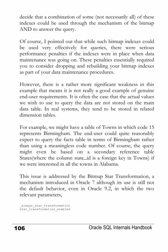
decide that a combination of some (not necessarily all) of these indexes could be used through the mechanism of the bitmap AND to answer the query. Of course, I pointed out that while such bitmap indexes could be used very effectively for queries, there were serious performance penalties if the indexes were in place when data maintenance was going on. These penalties essentially required you to consider dropping and rebuilding your bitmap indexesas part of your data maintenance procedures.

However, there is a rather more significant weakness in this example that means it is not really a good example of genuine end-user requirements. It is often the case that the actual values we wish to use to query the data are not stored on the main data table. In real systems, they tend to be stored in related dimension tables. For example, we might have a table of Towns in which code 15 represents Birmingham. The end-user could quite reasonably expect to query the facts table in terms of Birmingham rather than using a meaningless code number. Of course, the query might even be based on a secondary reference table States(where the column state_id is a foreign key in Towns) if we were interested in all the towns in Alabama. This issue is addressed by the Bitmap Star Transformation, a mechanism introduced in Oracle 7 although its use is still not the default behavior, even in Oracle 9.2, in which the two relevant parameters, _always_star_transformation star_transformation_enabled


still have the default value of FALSE. (Note: the star transformation is not the same as the star query that was introduced in earlier versions of Oracle 7 and was dependent on massive, multi-column b-tree indexes.) A new feature of Oracle 9.2, the bitmap join index, may also be of benefit in such queries, but the jury is still out on that one, and I plan to describe that mechanism and comment on it in a later feature.

The Bitmap Star Transformation What is a Bitmap Star Transformation, how do you implement it, and how do you know that it is working? The main components are a large fact table and a surrounding collection of dimension tables. A row in the fact table consists of a number of useful data elements, and a set of identifiers - typically short codes. Each identifying column has a bitmap index created over it. An identifying column on the fact table corresponds to one of the dimension tables, and the short codes that appear in that column must be selected from the (declared) primary key of that table. Figure 2 shows an extract from a suitable set of table definitions:

The Bitmap Star Transformation 107

Figure 2: Part of a Star (snowflake) Schema.

In this example, we have a people table as the central fact table, and a towns table, which is actually used twice as a dimension table. I have also included a states table representing the relationship that each town is in a state. This is to illustrate the fact that Oracle can actually recognize a "snowflake" schema. (Refer to figure 3.)


Figure 3: Simple Snowflake Schema. You will note that I have declared foreign key referential integrity between the people table and the towns table. There are two points to bear in mind here. First, that the presence of the bitmap index is not sufficient to avoid the share lock problem that shows up if you update or delete a parent id - an index created for this purpose has to be a b-tree index. (Of course, in a DSS database, such updates are not likely to be a significant issue.) Second, for reasons that will be discussed in future articles on materialized views and partitioned tables, such foreign key constraints in DSS databases are quite likely to be declared as disabled, not validated, and rely. Having created the tables, loaded them with suitable data, and then enabled the feature by issuing:


alter session set star_transformation_enabled = true;

we can start to examine the execution plans for queries such as those in figure 4.

Figure 4: Sample Queries.


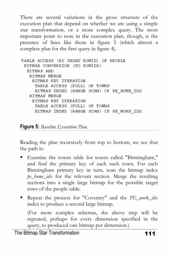
There are several variations in the gross structure of the execution plan that depend on whether we are using a simple star transformation, or a more complex query. The most important point to note in the execution plan, though, is the presence of lines like those in figure 5 (which almost a complete plan for the first query in figure 4).

Figure 5: Baseline Execution Plan.

Reading the plan recursively from top to bottom, we see that the path is: Examine the towns table for towns called "Birmingham,"

and find the primary key of each such town. For each Birmingham primary key in turn, scan the bitmap index pe_home_idx for the relevant section. Merge the resulting sections into a single large bitmap for the possible target rows of the people table. Repeat the process for "Coventry" and the PE_work_idx

index to produce a second large bitmap.

(For more complex schemas, the above step will be repeated, perhaps for every dimension specified in the query, to produced one bitmap per dimension.)


AND the two bitmaps together to produce a single bitmap identifying all people rows that match both conditions. Convert the resulting bitmap into a list of rowids, and fetch

the rows from the table. Notice how this stage of the operation, targets and returns the smallest possible set of people rows with the minimum expenditure of resources. Dimension tables are usually relatively small, so the cost of finding their primary keys is low; the bitmap indexes on the people table are relatively small, so scanning them for each towns key value is quite cheap, and the bitmap AND operation is very efficient. Remember — in many cases, the most expensive action in a query is the work of collecting the actual rows from the largest table(s). A mechanism like the bitmap star transformation that manages to identify exactly the bare minimum number of rows from the fact table, with no subsequent discards, can give you a terrific performance gain. Once we have established that the critical section of the plan is appearing, we can worry about the extra work that may have to be done. For example, in the second query in figure 4, we want columns from the towns table(s), as well as moving out one extra layer to get data from the states table. Because we have started with a star transformation to identify the critical people rows, we should now join this 'intermediate result set' back to the dimension tables with a minimum of extra work. So the questions we need to ask are - do we still see the same pattern of AND'ed bitmaps in the plan, and what can we see that shows us how the extra columns handled.


To answer the first question, the inner part of the plan now looks like figure 6. The same basic structure of the star transformation is clearly visible even though one (highlighted) part of it now includes a join to the states table. This is the critical section of code that ensures we locate the minimum set of people rows that are relevant, and use the minimum resources to get them.

Figure 6: Core of Extended Plan. What about the rest of the data, though — how does Oracle retrieve the extra columns that have not been required so far. The full plan — simplified by replacing the section shown in figure 6 by a single line — is likely to be something similar to the one shown figure 7:


Figure 7: Revisiting the Fact Tables.

The sub-plan shown above simply says — for each row found in the people table get the home town using the primary key, then get the work town by primary key, then get the state by primary key. In effect, the query has been rewritten internally in the form shown in figure 8, where we can more easily see the first half of the where clause becoming the driving bitmap access clause, and the second half of the clause being used to join back to the dimension tables.


Figure 8: Notional Internal rewrite. As ever, there are numerous variations on a theme. Oracle may be able to restructure b-tree information into

bitmap form in memory, so extra conversion steps may appear in the plan. The bitmap star transformation can be applied to

partitioned tables, so extra steps relating to partitioning may appear.


The path can execute in parallel, introducing extra levels of messy parallel distribution elements in the plan. The join back of the dimension tables could be

implemented as a series of hash joins, or sort merge joins instead of nested loop joins.

Warnings One important detail to watch out for is that the bitmap star transformation is available only to the Cost Based Optimizer (after all, the Rule Based Optimizer doesn't even recognize bitmap indexes). So, if you fail to generate statistics of a suitable quality, the optimizer may very easily switch into an alternative plan — typically a very expensive, multistage hash join mechanism. Of course, there is also the critical detail that you can't do the bitmap star transformation without using bitmap indexes, and these are only available with the Enterprise Edition. Also, be aware that under newer versions of Oracle, a recursive temporary table mechanism may be use to handle the dimension tables. At present tkprof, autotrace, and v$sql_plan have no method of showing you what is going on behind the scenes, so you will need the latest SQL code for reporting the results of an explain plan. For example, the second query of figure 4 might produce an autotrace plan including lines like those in figure 9:


Figure 9: Temp Table Transformation *extract).

You may be able to guess this has something to do with the join between (work) towns and states because those two tables will have vanished from the plan. But without the aid of the latest SQL for reporting the results of explain plan, you won't be able to see that the recursive step is creating and populating a temporary table using SQL, such as: INSERT INTO SYS.SYS_TEMP_0FD9D6605_333A5B SELECT WT.ID C0, WT.NAME C1, ST.NAME C2 FROM TEST_USER.STATES ST, TEST_USER.TOWNS WT WHERE ST.NAME='Alabama' AND WT.ID_STATE=ST.ID;

The same enhanced code for displaying execution paths will also show that, in this case, the generated SQL uses a hash join. (Hint: always check the rdbms/admin directory of your ORACLE_HOME for the scripts utlxpls.sql and utlxplp.sql, which produce outputs for serial and parallel execution plans respectively. These changed quite significantly for Oracle 9.0, and then switched to using a new package called dbms_xplan in Oracle 9.2.)

Warnings 117

It is possible, by the way, that in some special cases you will want to turn off the temporary table feature — there have been reports of circumstances in which the resource cost, particularly of memory or temporary space, becomes unreasonably high. If you hit this case, the star_transformation_enabled parameter has a third value (after true and false), which is temp_disable. This allows bitmap star transformations to take place, but disables the option for generating temporary tables.

Conclusion The bitmap star transformation is a very powerful feature for making certain types of query very efficient. However, the dependency on bitmap indexes does require that you have a proper strategy for data loading before you can take advantage of this high-performance query mechanism. You must also be aware that there are some very new features of explain plan that will require you to update your method for testing execution paths.


References Oracle 9i Release 2 Datawarehousing Guide, Chapter 17. Oracle 9i Release 2 Supplied Types and PL/SQL packages, Chapter 90 (DBMS_xplan). $ORACLE_HOME/rdbms/admin utlxplan.sql utlxpls.sql utlxplp.sql dbmsutil.sql

References 119

Bitmap Join Indexes CHAPTER

11 Bitmap Indexes 3 — Bitmap Join Indexes

In recent articles, I have described the functionality of bitmap indexes, and the bitmap star transformation. In this article we move on to the bitmap join index an option just introduced in Oracle 9. In the previous article in this short series on bitmap indexes, I described how ordinary bitmap indexes are used in the bitmap star transformation. In this article we look at the effect, and costs, of using the new bitmap join index in an attempt to make the process even more efficient. Figure 1 shows us a simple example of the way in which several tables might be related in a query that Oracle would address through the bitmap star transformation.


Figure 1: Simple snowflake schema. As we saw in my last article, the query represented by Figure 1 would be addressed by a two-stage process. First, Oracle would visit all the necessary outlying tables (the dimension tables and their parents) to collect a set of primary keys from each of the dimensions, which it could use to access the four bitmap indexes into the fact table. After ANDing the four bitmaps, to locate the minimum set of relevant fact rows, Oracle would 'turn around' to revisit the dimension tables and their parents — possibly using a nested loop access path through the primary keys on the outlying tables. Apparently, according to a whitepaper I found recently on Metalink, Oracle actually owns the copyright to some aspects of this extremely cute strategy.

Bitmap Indexes 3 — Bitmap Join Indexes 121

It's fantastic - What's the Problem There are three possible inefficiencies in this strategy (which, I have to add, seem to be very small compared to the massive benefit that the technology can introduce).

First — if the queries reaching the system are typically about some attribute of a dimension, but never acquire data about that dimension, then we are adding work by traveling through the dimension and perhaps merging many bitmap index sections corresponding to the selected primary keys from that dimension.

Secondly — if the queries reaching the system are typically aimed at the parent tables (the outer layers of the snowflake), then we are doing a lot of work tracking back and forth through the dimension tables.

Finally — bitmap indexes on columns of higher "distinct cardinality" can be relatively large; which leads to a waste of buffer space loading them, and a waste of memory and CPU if we have to merge lots of small bitmap ranges (see my first article on bitmap indexes to find out why the myth about "bitmaps for low-cardinality columns is misleading").

So — what has Oracle got to offer those of us whose systems are described by the conditions above? The answer is bitmap join indexes.

What Is a Bitmap Join Index? As its name suggests, this is a bitmap index, but an index that is described through a join query. Amazingly, it is an index where the indexed values come from one table, but the bitmaps point to another table.


Let's clarify this with a simple concrete example. Figure 2 reproduces the SQL I used to build my first demonstration of a star transformation:

Figure 2: Part of a star (snowflake) schema. Imagine now that I have observed that all the queries are about people who work in particular towns, and these towns are always referenced by name and not acquired by searching through attributes of the town. I may decide that the bitmap

What Is a Bitmap Join Index? 123

index on column (id_town_work) is sub-optimal, and should be replaced by a bitmap join index that allows a query to jump straight into the people table, bypassing the towns table completely. Figure 3 shows how I would define this index.

Figure 3: Creating a basic bitmap join index. Imagine that I have also noticed that queries about where people live are always based on the name of the state they live in, and not on the name of the town they live in. So the bitmap index on column (id_town_home) is even less appropriate, and could be replaced by a bitmap join index that allows a query to jump straight into the people table, bypassing both the states the towns tables completely. Figure 4 gives the definition for this index:

Figure 4: Creating a more subtle bitmap join index.


You will probably find that the index pe_work_id is the same size as the index it has replaced, but there is a chance that the PE_home_st_idx will be significantly smaller than the original PE_home_idx. However, the amount of space saved is extremely dependent on the data distribution and the typical number of (in this case) towns per state. In a test case with 4,000,000 rows, 500 towns, and 17 states, with maximum scattering of data, the PE_home_st_idx index dropped from 12MB to 9MB so the saving was not tremendous. On the other hand, when I rigged the distribution of data to emulate the scenario of loading data one state at a time, the index sizes were 8MB and 700K respectively. These tests, however, revealed an important issue. Even in the more dramatic space-saving case, the time to create the bitmap join index was much greater than the time taken to create the simple bitmap index. The index creation statements took 12 minutes 24 seconds in one case, and four minutes 30 seconds in the other; compared to a base time of one minute 10 seconds for the simple index. Remember, after all, that the index definition is a join of three tables. The execution path Oracle used to create the index appears in Figure 5.


Figure 5: Execution path for create index. As you can see, this example hashes the two small tables and passes the larger table through them. We are not writing an intermediate hash result to disc and rehashing it, so most of the work must be due to the sort that takes place before the bitmap construction. Presumably this could be optimized somewhat by using larger amounts of memory, but it is an important point to test before you go live on a full-scale system. At the end of the day, though, the most important question is whether or not these indexes work. So let's execute a query for people, searching on home state, and work town (refer to Figure 6 for the test query, and its execution plan). The query very specifically selects columns only from the people table. Note how the execution plan doesn't reference the towns table or the states table at all. It factors these out completely and resolves the rows required by the query purely through the two bitmap join indexes. The query:


Figure 6: Querying through a bitmap join index.

There is a little oddity that may cause confusion when you run your favorite bit of SQL to describe these indexes. Try executing: select table_name, column_name from user_ind_columns where index_name = 'PE_WORK_IDX';

The results come back as:

Oracle is telling you the truth - the index on the people table is an index on the towns.name column. But if you've got code that assumes the table_name in user_ind_columns always matches the table_name in user_indexes, you will find that your reports 'lose" bitmap join indexes. (In passing, the view user_indexes will have


the value YES in the column join_index for any bitmap join indexes).

Issues The mechanism is not perfect — even though it may offer significant benefits in special cases. "Join back" still takes place — even if you think it should be unnecessary. For example, if you changed the query in Figure 6 to select the home state, and the work town, (the two columns actually stored in the index, and supplied in the where clause) Oracle would still join back through all the tables to report these values. Of course, since the main benefit comes from reducing the cost of getting into the fact (people) table, it is possible that this little excess will be pretty irrelevant in most cases. More importantly, you will recall my warning in the previous articles about the dangers of mixing bitmap indexes and data updates. This problem is even more significant in the case of bitmap join indexes. Try inserting a single row into the people table with sql_trace set to true, and you will find some surprising recursive SQL going on behind the scenes — refer to Figure 7 for one of the two strange SQL statements that take place as part of this single row insert.


Figure 7: A recursive update to a bitmap join indexes. There are three new things in this one statement alone. First, the command upd_joinindex, which explain plan cannot yet cope with but which is known to Oracle as the operation "bitmapjoin index update." Second, the undocumented hint cardinality(), which is telling the cost based-optimizer to assume that the table aliased as T26763 will return exactly one row. And finally, you will notice that this SQL is nearly a copy of our definition of index PE_home_st_idx, but with the addition of table called SYS.L$15 — what is this strange table?

A little digging (with the help of SQL_trace) demonstrates the fact that every time you create a bitmap join index, Oracle needs at least a couple of global temporary tables in the SYS schema to support that index. In fact, there will be one global temporary table for each table referenced in the query that defines the index. These global temporary tables appear with names like L$nnn, and are declared as "on commit preserve rows." You don't have to worry about space being used in system tablespace, of course,

Issues 129

as global temporary tables allocate space in the user's temporary tablespace only as needed. Unfortunately, if you drop the index (as you may decide to do whenever applying a batch update), Oracle does not seem to drop all the global temporary table definitions. On the surface, this seems to be merely a bit of a nuisance, and not much of a threat - however, you may, like me, wonder what impact this might have on the data dictionary if you are dropping and recreating bitmap join indexes on numerous tables on a daily basis. If you pursue bitmap join indexes further through the use of SQL_trace — and it is a good idea to do so before you put them into production — you will also see accesses to tables sys.log$, sys.jijoin$, sys.jifrefreshsql$, and sequence sys.log$sequence. These are objects that are part of the infrastructure for maintaining the bitmap indexes. jirefreshsql$, for example, holds all the pieces of SQL text that might be used to update a bitmap join index when you change data in the underlying tables (you need a different piece of SQL for each table referenced in the index definition). Be warned every time that Oracle gives you a new, subtle, piece of functionality: there is usually a price to pay somewhere. It is best to know something about the price before you adopt the functionality.

Conclusion This article only scratches the surface of how you may make use of bitmap join indexes. It hasn't touched on issues with partitioned tables, or on indexes that include columns from multiple tables, or many of the other areas which are worthy of careful investigation. However, it has highlighted four key points.


Bitmap join indexes may, in special cases, reduce index sizes and CPU consumption quite significantly at query time.

Bitmap join indexes may take much more time to build than similar simple bitmap indexes. Make sure it's worth the cost. The overheads involved when you modify data covered by

bitmap join indexes can be very large — the indexes should almost certainly be dropped/invalidated and recreated/rebuilt as part of any update process — but watch out for the problem in the previous paragraph. There are still some anomalies related to Oracle's handling

of bitmap join indexes, particularly the clean-up process after they have been dropped.

References Oracle 9i Release 2 Datawarehousing Guide, Chapter 6.

References 131

Tracing SQL Execution

CHAPTER

12 Oracle_trace - the Best Built-in Diagnostic Tool?

Editor's Note: Shortly after this article was published, it came to light that the Oracle 9.2 Performance Guide and Reference has now identified Oracle Trace as a deprecated product.

There is a lot of diagnostic code built into the database engine some, such as sql_trace, is well documented and some, such as x$trace is undocumented. Every now and again, I like to spend a little time re-visiting areas of code like this to see how much they have evolved, and whether they have acquired official blessing and documentation. Recently, whilst doing some work with Oracle 9i, I discovered the amazing leap forward that oracle_trace has made in the last couple of releases. This article is a brief introduction to oracle_trace, and what it could do for you.

How Do I … ? Find out which object is the source of all the buffer busy waits that I can see in v$waitstat? We've all seen the tuning manuals: "if you see . . . you may need to increase freelists on the problem table" -- but no clue about how to find the problem table.

Option 1 - run a continuous stream of queries against v$session_wait and check the values of p1,p2, p3 when this event appears. Statistically you will eventually get a good indicator of which object(s) are causing the problem. A bit of a pain to do, and relies a little on luck.


Option 2 - switch on event 10046 at level 8, and catch a massive stream of wait states in trace files. A fairly brutal overhead, and again relies on a little bit of luck.

Option 3 - there is an event (10240) which is supposed to produce a trace file listing the addresses of blocks we wait for (hooray!), but I've not yet managed to get it to work. If you do know how to, please let me know, as this is clearly the optimum solution.

So would you like to get a list of just those blocks we wait for, who waited for them, why they waited, and how long they waited - at minimal cost? This is just one of the things that oracle_trace can do for you.

What is oracle_trace oracle_trace is a component of the database engine that collects events, apparently at relatively low cost. Events include such things as waits, connects, disconnects, calls to parse, execute, fetch, and several others. You can collect the information from the entire instance or target specific users, events, or processes; and can switch the tracing on and off at will. But one of the really nice features of oracle_trace is that it can be set to buffer the collection and dump it to disc in big chunks, rather than leaking it out a line at a time. Not only that, but you can request that the collection file should be a fixed size, and should be recycled. Naturally, once you have generated a collection file, you need to analyze it. You can do this one of two ways - run a program

What is oracle_trace 133

that converts the collection file into a series of flat text reports, or run a program that reads the collection file and dumps it into a set of Oracle tables, from which you can then generate your own reports.

Uses for oracle_trace So how does oracle_trace help us to answer the original question? Simple: one of the classes of events that can be traced is waits. We ensure that we have started our database in a ready to trace mode, and then tell Oracle, either through PL/SQL or the command line interface, to start tracing waits. But we restrict the choice of wait events to just wait 92 (this is buffer busy waits in my Oracle 9i system, but check event# and name from v$event_name for your system). We then sit back and wait for an hour or so at peak problem time. When we think our trace file is large enough, we stop tracing, format the trace file into a database, and run an SQL statement that might, for example, say something like,

tell me which objects are subject to buffer busy waits, the wait time, how often it happens and who got hit the most.

If we wanted to suffer an extra overhead, we could even start a trace to capture the waits and the SQL, and get a report of the SQL that suffered the waits.

Putting it All Together The first component of our task is to set some database parameters so that the database is ready to trace, but not tracing. Fig.1 shows the list.


REQUIRED

oracle_trace_enable = true oracle_trace_collection_name = **

DEFAULTS

oracle_trace_collection_size = 5242880

oracle_trace_collection_path = ?/otrace/admin/cdf oracle_trace_facility_path = ?/otrace/admin/fdf oracle_trace_facility_name = oracled

Figure 1: Parameters relating to oracle_trace The oracle_trace_collection_name must be set to an explicit blank "" otherwise it defaults to "oracle," and if there is a collection name available, when trace is enabled then Oracle does instance level tracing from the moment it starts up (ouch!). The oracle_trace_collection_path is the directory where the files will go. The oracle_trace_facility_path is where the lists of events to be traced (facility definition files supplied by Oracle Corporation) will be located. The oracle_trace_facility_name identifies the list of events we are interested in. Finally we can limit the size (in bytes) of the collection file using oracle_trace_collection_size.

Putting it All Together 135

Once the database is started, we can start a trace collection. In this article I will stick with using the command line interface, although there is a PL/SQL interface as an alternative (and a graphic interface if you purchase the module for Oracle Enterprise Manager). The command we use will be something like: otrccol start 1 otrace.cfg

The otrccol command is the primary interface to oracle_trace. There are other commands, but their functionality has generally been added to otrccol. Obviously we use start to start tracing (and stop to stop tracing). The "1" is an arbitrary job id, and otrace.cfg is a configuration file. See figure 2 for an example of a configuration file. USED FOR COLLECTION

col_name = jpl cdf_file = jpl dat_file = jpl fdf_file = waits.fdf max_cdf = -10485760 buffer_size = 1048576 regid = 1 192216243 7 92 5 d901

USED FOR FORMATTING

username = otrace password = otrace service = d901 full_format = 1

Figure 2: Sample oracle_trace configuration file.


This file tells oracle to produce a collection file called jpl.dat, with a collection definition file called jpl.cdf, and a collection identifier of jpl. The facility definition is in the file waits.fdf(supplied by Oracle Corp. to identify wait events only). The trace file will be limited to 10 MB, but will be recycled so that there is always 10MB of recent data in it, and Oracle will use a buffer of 1MB to hold data before dumping it.

The regid is one of the really powerful features of oracle_trace. The 'default' value for this line reads '0 0' where I have the values '7 92', and in its default form the line states that oracle_trace is tracing across the entire Oracle instance identified by the d901 at the end of the line. In the form shown, I have chosen to trace only facility number 7 (wait events) facility item 92 (buffer busy waits). You can have multiple regid lines in a file if you want to. For my first set of experiments, I used two regid lines in my configuration file, specifying '7 129' and '7 130' - sequential and scattered reads respectively, as these types of waits are easy to generate. I will mention the formatting section later in the article. After letting the system run for a while, we then execute: otrccol stop 1 otrace.cfg otrccol format otrace.cfg

The first command stops the trace, the second command reads the collection file and dumps it into a set of Oracle tables.

Putting it All Together 137

However, before you can format the collection, you need to create an account to hold the tables used by the formatter. For the name and password we use the values listed in fig.2 above.

The significance of the full_format=1 line in the configuration file is that it forces the formatter to dump the entire file to table, full_format=0 would restrict the task to new data only. Note also the service name -- this identifies the database that holds the account -- you will need the TNS listener running to use the format command, even if you format to the local database.

Figure 3 shows a short script to create the account and give it suitable privileges. create user otrace identified by otrace default tablespace users -- if you are not using 9i -- temporary tablespace temp quota 100m on users; grant create session to otrace; grant create table to otrace; grant create sequence to otrace; grant create synonym to otrace;

Figure 3: Creating a user for the trace tables. When you run the format option, the program will automatically (at least in newer versions of Oracle) create the necessary target tables under the supplied account. Some of these tables will have sensible names like: EPC_COLLECTION

Others will be meaningless things such as: V_192216243_F_5_E_9_9_0

The problem of incomprehensibility can be addressed by running script otrcsyn.sql in directory $ORACLE_HOME/otrace/demo.


This script produces synonyms for the tables, giving them meaningful names such as WAIT CONNECTION

(There are variations in names across different versions of Oracle.) I found a small problem with the automatic table generation. If you use one of the very selective lists of facilities (such as waits.fdf) only the set of tables required for the resulting data appears when you format the data. If you then decide to use a more comprehensive list of facilities (such as oracle.fdf) the formatter will get confused and crash because some tables are present and some are missing. So it may help to run for just a few seconds with facility oracle.fdf, format the data, then truncate all the tables. This is a crude, but effective, method for setting up the account.

Some Results So finally what have we done: Created a config file Started a collection Done some work on the database Stopped the collection Formatted the collection

Now What? Assume we have been using the configuration file from figure 2. We would find, when we logged into the otrace account, that

Some Results 139

we had some rows in the connection, disconnect, and wait tables. The rows in the wait table would tell us all about the buffer busy waits in the interval we traced For example, we could execute the SQL in figure 4: select p1 file_id, p2 block_id, p3 reason_code, count(*) ct, sum(time_waited)/100 secs from wait group by p1, p2, p3 order by sum(time_waited) desc ;

Figure 4: Sample query to identify worst BBWs.

If you want greater precision, you can list all the waits, with timestamp, and a column called (optimistically perhaps) timestamp_nano. If you want to identify users with the worst wait problem, change the query to sum by session_index (SID) and session_serial (serial#). The table (synonyms) connection can be used to turn (session_index, session_serial) into the username, machine name, logon time, and so on. Of course, there's nothing (except performance costs) stopping you from joining this table to the dba_extents view to translated file and block ids into object types and names. And if you want to locate the specific SQL that suffered the waits you can always, at a rather higher cost of course, switch to the sql_waits.fdf file, which populates a few more of the trace


tables, then join them on session_index, session_serial, timestamp, and timestamp_nano. Finally, if you are worried that the cost of loading the data into tables and running the reports will have a negative impact on the system, you can always move the cdf and dat files to another machine and process them in another database. I even managed, with just a little fixing, to generate collection data on a version 9i instance, and then process it on a version 8i instance, just to prove the point. This would, of course, restrict your ability to associate blocks with objects.

The Future The possibilities are endless - for example, one of the facility definition files is called oraclec.fdf and this tracks buffer cache activity. After tracing this, you can actually report, pretty much to the micro second, the blocks that were loaded into the cache, in the order they were loaded, and which blocks they pushed out in order to be loaded. (I suspect the overhead is likely to be a bit too painful for general use.) Another option that is likely to be generally useful is the connect.fdf file. This captures session connects and disconnects, in much the same way that the command audit session will do. However, the trace file collects half a dozen extra session statistics (such as redo entries) which are not collected in the aud$ table; and it isn't writing to the database as it does so. And for that very special individual - you can even set oracle_trace to target just one user. You could even write SQL to read the resulting tables, and generate an exact clone of a normal sql_trace file, with the added benefit of being able to

The Future 141

track from the moment they log in, migrate across multi-threaded servers, and finally log out.

Conclusion This is just a brief introduction to oracle_trace that barely scratches the surface of how you can use it. There is still some work to do in determining the stability and side effects of oracle_trace, not to mention the performance impact. However, initial investigations suggest that it is much cheaper than other built-in diagnostics, and much more flexible and precise in what it can report. At the very least, it allows you to get some accurate answers to some of the vexing questions that have plagued DBAs over the years. Personally I wouldn't be particularly surprised if oracle_trace didn't end up replacing just about every other diagnostic strategy some time within the next couple of years.

Caveat There are a number of differences, usually in nothing other than names, between the Oracle 8i and the Oracle 9i implementation of oracle_trace. This article was written purely from the perspective of Oracle 9i.

References Oracle 9i Performance Tuning Guide and Reference, Chapter 12.


Embedding SQL in Java & PL/SQL

CHAPTER

13 Java vs. PL/SQL: Where Do I Put the SQL?

Note: The Source Code file that accompanies this article contains the following: Lab1.sql-PL/SQL package header spec Lab1body.sql-PL/SQL package body definition Lab1.java-Java test application

Many articles have been written about the use of PL/SQL vs. Java. These articles tend to focus on the intricacies of each language and their strengths and weaknesses as the server-side logic. This article won't focus on this issue but will instead concentrate on an issue that faces Java and PL/SQL developers alike -- where do you put the SQL? The SQL is a major part of each application, and its location can greatly enhance or degrade performance, distribution, and maintenance. Java is certainly mainstream at this point and is a very powerful language. Even though it's a personal favorite of this author, it still has its disadvantages. PL/SQL, while obviously database-centric (Oracle), also has some enormous benefits. Good developers use both where appropriate and often find themselves perplexed with the same issue -- the location of the SQL statements. When I say "the location of the SQL," I'm referring to its storage location. The developer has many options when writing Java applications, servlets, and applets that access databases.

Java vs. PL/SQL: Where Do I Put the SQL? 143

You can store SQL in the application itself (Java side) and access the database directly from the applet via a SQL statement. Or the programmer can make a request from the applet to the servlet, which then sends the SQL to the database. Another option within Java is to simply make a procedure or function call (Callable Statement in JDBC Driver) and process the result set. In the last scenario, the SQL would reside inside the database in an Oracle package. This article explores the advantages and disadvantages of these options and includes performance benchmarks. It's my intention to objectively answer my own questions while helping to make your decision easier when you encounter this issue in your own projects.

The Power of a Package If you have the option of installing a PL/SQL package as part of your application, you should seriously consider installing it. (Although the focus of this article is on PL/SQL, the package could also be written in Java in versions of Oracle 8.1 and later.) PL/SQL packages have many advantages: Privilege Management-Instead of being concerned about

whether each user has the rights to perform a function and trapping exceptions throughout your code, you can grant execute on a package. The user inherits rights to all of the underlying objects indirectly through package execution. For example, let's assume that part of your code issued a TRUNCATE command on a table. If the command is issued as the connected user, you can expect privilege problems and would need to resolve these problems by granting the proper privileges to the user. You would either have to connect as someone with privileges behind the scenes or put the TRUNCATE command in a procedure call in the package. The procedure becomes the gatekeeper


of the transaction and ensures that any access to the underlying objects goes through the procedure. Global Location-Having the SQL in one spot is the most

flexible option: By having calc_inventory() as a procedure call, any application that can issue a database call can benefit from the procedure. Your Java apps, applications, Oracle*Forms, Visual Basic, or any application that can issue a SQL statement can easily access the same result because it's the same code that produces the result. This solution is preferable to reproducing the same algorithm in different code bases maintained by different people. And it surpasses trying to access methods in one language from the architecture of another by leveraging APIs and RPCs-a strategy that's more complex to build and maintain. Put the SQL in the database and be done with it. Performance-Most of the time, performance will be the

driving issue in the decision of how to partition an application. Very few users are interested in elegant architectures when their query takes five minutes to return after they clicked a button. The fact is that you can't run a SQL statement any faster than running it inside the Oracle kernel. But at what point is performance really an issue? Is a package faster when submitting a single SQL statement? Or is it only when submitting two or more that a package is faster? When is it clearly the best solution for performance reasons? I'll show later in this article that PL/SQL is faster with some tasks and slower with others. Interface Agnostic-Software architects learned long ago that

it makes sense to separate back-end logic from the interface. Interface technologies change much more frequently than databases. Whether it's Java Swing, AWT, Visual Basic, PowerBuilder, or Oracle*Forms, a well-designed application

The Power of a Package 145

can support them all. Decouple the business logic from the user interface controls and you're well on your way. Global Variables-Global variables are useful, and yes, Java

has static variables as well. The difference is that global package variables apply to anyone who accesses them regardless of the application. This allows you to maintain data across and between transactions through persistent data. A user in SQL*Plus, JDBC, Java, Visual Basic, and ODBC will inherit the performance benefits. The following code shows an example since it only calculates the global cost when the global cost variable hasn't been set (=0). Function x returns VARCHAR2 BEGIN If global_cost = 0 then -- global_cost is defined outside the scope Calc_global_cost(); -- (first time in only) endif; END

The Flexibility of Java Java also has some benefits as a home for your Oracle SQL statements. These benefits include: Simplicity-Embedding SQL statements in native Java code

is much easier than building additional pieces, like PL/SQL packages. Debugging-Although tools exist that enable the debugging

of PL/SQL, they're less robust than the functionality in existing Java IDEs, like JBuilder. Being able to set breakpoints and inspect variable values is a critical requirement for any developer, and it's preferable to do that from a single development environment. Distribution-Having the code encapsulated in one place

makes the distribution and management of the application much easier. If a user can simply access a URL and use your


application instantly, then you have a satisfied user. If you create a package in the database, you'll have to install that package in each database to be accessed. By keeping the SQL in the Java code, you can connect to any database and don't have to worry about PL/SQL package maintenance on each node. Performance-When performing many inserts or updates,

Java performs better because it has the ability to batch these statements. The JDBC driver provides the ability to queue the request and when the number of queued requests reaches the batch size, JDBC sends them to the database for execution.

Performance At first glance, the main performance degradation for a SQL request is sending and receiving the request across the network. We also know that most boosts in performance rely on the architect eliminating or reducing the number of round trips to the database. A logical assumption is that batching requests and then sending them as a group would greatly enhance performance. But how much does it enhance performance? And what's the threshold that seems to be the decision point? Is a single statement faster in a package? Two statements? Or is it only when you have 25-50 statements that a package becomes the ideal choice? These are the questions that I hope to answer in the benchmark tests in the following section.

Benchmarks The timings for these benchmark tests are given in milliseconds and are calculated by making the call System.currentTimeMillis() in

Performance 147

the Java code. Each test was performed 10 times, and the average result is reported. Each test was performed locally, over an internal network, and remotely, over a broadband connection (DSL).

Environment Database: Oracle 8.1.5 on HP-UX B.11.00 A 9000/785 JDBC Driver: Oracle Thin 8.1.6.0 Client machine: Pentium II NEC Laptop 366 MHz with 256MB RAM Java Virtual Machine: 1.3.0_01

The Tests My test scenarios consisted of timing the particular statements during their execution only. I tried to eliminate the definition of the statement as well as processing and closing of any result sets. You'll notice in the Java code that the clock is started right before the execute statement and stopped after it returns. I also used prepared statements in my tests instead of regular statements. It's more efficient to use PreparedStatement with bind variables for frequently executed statements. Although PreparedStatement is inherited from Statement, it's different in the following two ways: Each time you execute a Statement object, its SQL

statement is compiled. However, when you execute a PreparedStatement, its SQL statement is only compiled when you first prepare the PreparedStatement. You can specify parameters in the PreparedStatement SQL

string, but not in a Statement SQL string. Single statement:


The single statement test is a very simple test. I tried to create a statement that everyone could run on their machines, and one that wouldn't be answered immediately to ensure that the time reported wasn't solely network communication time. At the time I ran this query, I had 3,194 objects reported in DBA_OBJECTS (see Listing 1).

Java: SQLText = "select count(*) from dba_objects"; pstmt = databaseConnection.prepareStatement(SQLText); startTime = System.currentTimeMillis(); ResultSet rs = pstmt.executeQuery(); rs.next(); x = rs.getString(1);

PL/SQL: FUNCTION single_statement RETURN VARCHAR IS row_count PLS_INTEGER := 0; BEGIN select count(*) into row_count from dba_objects; return row_count; END single_statement;

Listing 1: The single statement test.

Multiple Statements The multiple statement test was a bit more difficult. At first, I used 10 different queries. Later I decided to use the same query 10 times and place it in a loop instead of coding it 10 times (see Listing 2).

Java: SQLText = "select count(*) from dba_objects"; pstmt = databaseConnection.prepareStatement(SQLText); ResultSet rs = null; startTime = System.currentTimeMillis(); while (multiCount < 10) { rs = pstmt.executeQuery(); /*

Multiple Statements 149

don't include result set processing in the timings since we do not do it in the PL/SQL rs.next(); x = rs.getString(1); */ multiCount ++; } multiStatementJava = multiStatementJava + System.currentTimeMillis() - startTime;

PL/SQL: FUNCTION multiple_statements RETURN VARCHAR IS row_count PLS_INTEGER := 0; num_objects VARCHAR2(20); BEGIN WHILE row_count < 10 LOOP select count(*) into num_objects from dba_objects; row_count := row_count + 1; END LOOP; return row_count; END multiple_statements;

Listing 2: The multiple statement test.

Truncate The truncate test simply truncates a table. No result set is involved. I included this test to observe the benchmarks when no rows are returned (see Listing 3).

Java: SQLText = "TRUNCATE TABLE SOOTHSAYER.BMC$PKK_INSTANCE_STATS"; pstmt = databaseConnection.prepareStatement(SQLText); startTime = System.currentTimeMillis(); ResultSet rs = pstmt.executeQuery(); truncateJava = truncateJava + System.currentTimeMillis() - startTime;


PL/SQL: Procedure truncate_table IS trunc_command varchar2(100); BEGIN trunc_command := 'TRUNCATE TABLE BMC$PKK_INSTANCE_STATS'; execute immediate (trunc_command); END truncate_table; Java Oracle package

Listing 3: The truncate test.

Benchmark Results The following table shows the average local test results, in milliseconds, for each type of test:

DB ON HP MACHINE JAVA ORACLE PACKAGE Single statement 47 48 Multiple statements 448 376 TRUNCATE 88 82

Single Statement Results The single statement test shows nearly equal results after 10 executions. The difference of 1 ms seems negligible (although the remote test provides a very different result). I was a bit surprised at how close these two results were, so I decided to see how much time was spent going to the server and not executing the SQL statement. I did this by commenting out the one line of work in the function: FUNCTION single_statement RETURN VARCHAR IS row_count PLS_INTEGER := 0; BEGIN -- select count(*) into row_count from dba_objects; return row_count; END get_row_count;

Benchmark Results 151

It took an average of 8 ms (~16% of total execution time) to access the procedure and return, without actually executing the

statement. This result tells me that each trip I can eliminate will save 8 ms.

Multiple Statements Results The results of the multiple statement test confirm my assumption. The Oracle package is faster because it makes one trip to the database, does its work, and then returns. This result clearly shows that a package should be used when the complete unit of work can be performed on the database. Larger units of work will result in more significant performance gains. To determine whether any overhead was incurred because the procedure was inside a package, I eliminated the package and created a stand-alone procedure. The results showed no impact; the numbers were the same.

Truncate Results The results of the truncate test were surprising-the execution is actually faster in Java than in PL/SQL. Oracle must be eliminating some overhead in the JDBC driver that isn't eliminated in PL/SQL.

Remote Results The following table shows the average remote test results, in milliseconds, for each type of test:

HP MACHINE VIA BROADBAND CONNECTION (DSL)

JAVA ORACLE PACKAGE

Single statement 286 113 Multiple statements 1662 506 TRUNCATE 217 332


The test results from the broadband connection are revealing: A 1 ms difference in the single statement test equates to 173

ms with a slow connection speed. The results of the multiple statement test are overwhelming,

showing that the PL/SQL package is three times faster. Once again, the TRUNCATE command is faster in Java

than in PL/SQL. Although we might easily discount a difference of a few milliseconds as being "close enough," as in the first single statement test, the remote test shows that we should always consider the faster approach. A query that executes only 5 ms slower in Java than in a PL/SQL package (or vice versa) might not seem like an issue. However, if the query is executed 5,000 times per day, that difference affects performance considerably. Also consider that the difference of 5 ms might occur when you're testing the code at work on a T1 line with the server three feet from your desk. But when you test the code over an ISDN, cable, or DSL connection, that 5 ms can become 55 ms or 300 ms. Every millisecond counts when performance tuning.

Conclusion It's hard to declare a clear winner in this topic. Many factors demand a combination of strategies. The ultimate decision should weigh the following factors and their applicability to the application: Unit of Work (UOW)-If the UOW is one SQL statement,

then creating a function solely for it makes little sense. However, if the unit of work is a series of SQL statements with processing in between, a package might provide the best solution. This solution assumes that:

Conclusion 153

o the Graphical User Interface doesn't need to be informed of the status of the work, as is typical in a progress bar of a GUI control; and

o the database can perform all processing required. Network Speed-We witnessed the impact of running the

same program over the internal network vs. a DSL connection. If network speed becomes an issue, the use of the package is preferable. Database Accessibility-If the application gives the option to

connect to any database or a large number of databases, having the code in the Java eliminates the distribution and maintenance of the package. All of the code used in the tests is available in the Source Code file at www.oracleprofessionalnewsletter.com and can be used as a template to test your SQL statements in your environment. MOORE.ZIP at www.oracleprofessionalnewsletter.com


Matrix Transposition in Oracle SQL

CHAPTER

14 Matrix Transposition in SQL

Matrix transposition is among Frequently Asked Questions. Given a single-column table ORIGINAL, ENAME SMITH ALLEN WARD JONES MARTIN BLAKE CLARK SCOTT KING TURNER ADAMS JAMES FORD MILLER

we’ll explore how to transform it into TRANSPOSED: Column S A W J M B C S K T A J F M M L A O A L L C I U D A O I I L R N R A A O N R A M R L T E D E T K R T G N M E D L H N S I E K T E S S E N R R

This problem has been discussed in the Usenet thread Matrix transpose in SQL, and general agreement was that it can’t be done in standard SQL-92. One of the latest oracle magazine code tips -- "Transposing a Table into a Summary Matrix" -- suggests a rather lengthy procedural solution. This article describes a SQL solution with a minimal amount of procedural

Matrix Transposition in SQL 155

code. As a bonus, we’ll learn several ways how to program user-defined aggregates in Oracle 9i.

Nesting and Unnesting Consider the table EMPNO POS LET 7369 1 S 7369 2 M 7369 3 I 7369 4 T 7369 5 H 7499 1 A 7499 2 L 7499 3 L 7499 4 E 7499 5 N … … …

that we call UNNESTED. Both tables in the beginning of the article could be viewed as aggregates of UNNESTED. The ORIGINAL table could be specified as: select concat(LET) from UNNESTED group by EMPNO

while the TRANSPOSED table is just a grouping by a different column: select concat(LET||’ ‘) from UNNESTED group by POS

(I also added a space padding to make the query result set more readable). So the problem of transposing the ORIGINAL table into TRANSPOSED can be solved by just implementing two steps: Unnesting ORIGINAL --> UNNESTED Nesting UNNESTED --> TRANSPOSED

The first step involves an integer enumeration relation, introduced in my previous article. Reader feedback, and other


articles about integer enumeration convinced me to further expand on this topic.

Integer Enumeration for Aggregate Dismembering Again, I prefer producing arbitrary, large list of integers with a Table Function CREATE TYPE IntSet AS TABLE OF Integer; / CREATE or replace FUNCTION UNSAFE RETURN IntSet PIPELINED IS BEGIN loop PIPE ROW(1); end loop; END; / select rownum from TABLE(UNSAFE) where rownum < 1000000 select rownum from TABLE(UNSAFE) where rownum < 1000000

In my previous article, I reserved the possibility of using an upper-bound integer range argument that would make the function safe. In other words, the function would never spin out of control whenever a user forgot the stop predicate rownum < 1000000. On the other hand, using the function argument is inferior for two reasons: predicates are more self-documenting than function

arguments, and we can use subqueries instead of hardcoded limits.

The runtime expense of using the table function is minimal: unlike forced materialization into a real table, logical I/O associated with table function calls is virtually zero. In DB2, a list of integers can be constructed with recursive SQL:

Integer Enumeration for Aggregate Dismembering 157

with iota (n) as ( values(1) union all select n+1 from iota where n<100000 ) select * from iota;

It is slightly inconvenient, however, that the predicate, which limits the list of numbers, must be specified within the recursion subquery, while it naturally belongs to the main query. The problem of pushing the predicate inside an inner query is somewhat similar to the one we saw for UNSAFE table function. With the list of integers at our disposal, writing an unnesting query is easy: SQL>select empno, pos, substr(ENAME,i,1) from emp, 2 (select rownum pos from table(unsafe) 3 where rownum < (select max(length(ename)) from emp)); EMPNO POS S ---------- ---------- - 7369 1 S 7369 2 M 7369 3 I 7369 4 T 7369 5 H 7499 1 A 7499 2 L 7499 3 L 7499 4 E 7499 5 N 7521 1 W

Looking at strings "SMITH," "ALLEN," etc., as aggregates of letters might seem odd at first, but that is what they really are. We’ll assemble those letters back into aggregates of (different) words.


User Defined Aggregate Functions There is no aggregate function that would concatenate strings in standard SQL. However, there are multiple ways defining it in Oracle: Casting the subquery result set into the collection and the

defining aggregate on it Pipelining the user-defined aggregate function:

CREATE or replace FUNCTION CONCAT_LIST( cur SYS_REFCURSOR ) RETURN VARCHAR2 IS ret VARCHAR2(32000); tmp VARCHAR2(4000); BEGIN loop fetch cur into tmp; exit when cur%NOTFOUND; ret := ret || tmp; end loop; RETURN ret; END; /

select distinct deptno, CONCAT_LIST(CURSOR( select ename ||',' from emp ee where e.deptno = ee.deptno ) employees from emp e;

Syntactically, neither of these solutions looks like a group by. However, scalar subquery in the select list is actually more powerful than group by. This idea is emphasized in the article by C.J.Date: "A discussion of some redundancies in SQL." If you prefer, however, the traditional group by syntax, then there is yet another way to program user-defined aggregates: Oracle 9i user-defined aggregates:

create or replace type string_agg_type as object ( total varchar2(4000), static function ODCIAggregateInitialize(sctx IN OUT string_agg_type ) return number,

User Defined Aggregate Functions 159

member function

ODCIAggregateIterate(self IN OUT string_agg_type , value IN varchar2 ) return number, member function ODCIAggregateTerminate(self IN string_agg_type, returnValue OUT varchar2, flags IN number) return number, member function ODCIAggregateMerge(self IN OUT string_agg_type, ctx2 IN string_agg_type) return number ); / create or replace type body string_agg_type is static function ODCIAggregateInitialize(sctx IN OUT string_agg_type) return number is begin sctx := string_agg_type( null ); return ODCIConst.Success; end; member function ODCIAggregateIterate(self IN OUT string_agg_type, value IN varchar2 ) return number is begin self.total := self.total || value; return ODCIConst.Success; end; member function ODCIAggregateTerminate(self IN string_agg_type, returnValue OUT varchar2, flags IN number) return number is begin returnValue := self.total; return ODCIConst.Success; end; member function ODCIAggregateMerge(self IN OUT string_agg_type, ctx2 IN string_agg_type) return number is begin self.total := self.total || ctx2.total; return ODCIConst.Success; end; end; /


CREATE or replace FUNCTION stragg(input varchar2 ) RETURN varchar2 PARALLEL_ENABLE AGGREGATE USING string_agg_type; / select deptno, stragg(ename) from emp group by deptno;

This last solution is probably the best from a performance perspective, since the query with the user-defined aggregate looks exactly like the traditional group by, the usual optimizations can be employed. Compare this to the second method -- pipelining the user-defined aggregate function. In that case the optimizer would certainly not be able to unnest a scalar subquery within a table function (yet). Now we have all the ingredients necessary for writing the transposition query. According to our program, we need to apply aggregation to the unnested view. I skipped that step, however, and rewrote the query directly to select CONCAT_LIST(CURSOR( SELECT substr(ENAME,i,1)|| ' ' from emp )) from (select rownum i from table(unsafe) where rownum < (select max(length(ename))+1 from emp))

Here I used solution #2 for user defined aggregates, and the reader is advised writing a transposition query with the other aggregate solutions as well. The last query needs the final touch: taking care of those employee names, which are shorter than the maximum length. It can be easily accommodated with a switch:

User Defined Aggregate Functions 161

select CONCAT_LIST(CURSOR( select case when length(ename)<i then ' ' else substr(ENAME,i,1)|| ' ' end from emp )) from (select rownum i from table(unsafe) where rownum < (select max(length(ename))+1 from emp)) CONCAT_LIST(CURSOR(SELECTCASEWHENLENGTH(ENAME --------------------------------------------- S A W J M B C S K T A J F M M L A O A L L C I U D A O I I L R N R A A O N R A M R L T E D E T K R T G N M E D L H N S I E K T E S S E N R R


SQL with Keyword Searches

CHAPTER

15 Keyword Searches

Here is a short problem that you might like to play with. You are given a table with a document number and a keyword that someone extracted as descriptive of that document. This is the way that many professional organizations access journal articles. We can declare a simple version of this table. CREATE TABLE Documents (document_id INTEGER NOT NULL, key_word VARCHAR(25) NOT NULL, PRIMARY KEY (document_id, key_word));

Your assignment is to write a general searching query in SQL. You are given a list of words that the document must have and a list of words which the document must NOT have. We need a table for the list of words which we want to find: CREATE TABLE SearchList (word VARCHAR(25) NOT NULL PRIMARY KEY);

And we need another table for the words that will exclude a document. CREATE TABLE ExcludeList (word VARCHAR(25) NOT NULL PRIMARY KEY);

Breaking the problem down into two parts, excluding a document is easy. CREATE TABLE ExcludeList

Keyword Searches 163

(word VARCHAR(25) NOT NULL PRIMARY KEY);

Breaking the problem down into two parts, excluding a document is easy. SELECT DISTINCT document_id FROM Documents AS D1 WHERE NOT EXISTS (SELECT * FROM ExcludeList AS E1 WHERE E1.word = D1.key_word);

This says that you want only the documents that have no matches in the excluded word list. You might want to make the WHERE clause in the subquery expression more general by using a LIKE predicate or similar expression, like this. WHERE E1.word LIKE D1.key_word || '%' OR E1.word LIKE '%' || D1.key_word OR D1.key_word LIKE E1.word || '%' OR D1.key_word LIKE '%' || E1.word

This would give you a very forgiving matching criteria. That is not a good idea when you are excluding documents. When you wanted to get rid "Smith" is does not follow that you also wanted to get rid of "Smithsonian" as well. For this example, Let you agree that equality is the right matching criteria, to keep the code simple. Put that solution aside for a minute and move on to the other part of the problem; finding documents that have all the words you have in your search list. The first attempt to combine both of these queries is:


SELECT D1.document_id FROM Documents AS D1 WHERE EXISTS (SELECT * FROM SearchList AS S1 WHERE S1.word = D1.key_word); AND NOT EXISTS (SELECT * FROM ExcludeList AS E1 WHERE E1.word = D1.key_word);

This answer is wrong. It will pick documents with any search word, not all search words. It does remove a document when it finds any of the exclude words. What do you do when a word is in both the search and the exclude lists? This predicate has made the decision that exclusion overrides the search list. The is probably reasonable, but it was not in the specifications. Another thing the specification did not tell us is what happens when a document has all the search words and some extras? Do we look only for an exact match, or can a document have more keywords? Fortunately, the operation of picking the documents that contain all the search words is known as Relational Division. It was one of the original operators that Ted Codd proposed in his papers on relational database theory. Here is one way to code this operation in SQL. SELECT D1.document_id FROM Documents AS D1, SearchList AS S1 WHERE D1.key_word = S1.word GROUP BY D1.document_id HAVING COUNT(D1.word) >= (SELECT COUNT(word) FROM SearchList);

Keyword Searches 165

What this does is map the search list to the document's key word list and if the search list is the same size as the mapping, you have a match. If you need a mental model of what is happening, imagine that a librarian is sticking Post-It notes on the documents that have each search word. When she has used all of the Post-It notes on one document, it is a match. If you

want an exact match, change the >= to = in the HAVING clause. Now we are ready to combine the two lists into one query. This will remove a document which contains any exclude word and accept a document with all (or more) of the search words. SELECT D1.document_id FROM Documents AS D1, SearchList AS S1 WHERE D1.key_word = S1.word AND NOT EXISTS (SELECT * FROM ExcludeList AS E1 WHERE E1.word = D1.key_word) GROUP BY D1.document_id HAVING COUNT(D1.word) >= (SELECT COUNT(word) FROM SearchList);

The trick is in seeing that there is an order of execution to the steps in process. If the exclude list is long, then this will filter out a lot of documents before doing the GROUP BY and the relational division.


Using SQL with Web Databases

CHAPTER

16 Web Databases

An American thinks that 100 years is a long time; a European thinks that 100 miles is a long trip. How you see the world is relative to your environment and your experience. We are starting to see the same thing happen in databases, too. The first fight has long since been over and SQL won the battle for a standard database language. However, if you look at the actual figures, only 12 percent of the world's data is in SQL databases. If a few weeks is supposed to be an "Internet Year," then why is it taking so long to convert legacy data to SQL? The simple truth is that you could probably pick any legacy system and move its data to SQL in a week or less. The trouble is that it would require years, maybe decades, to convert the legacy applications code to a language that could use the SQL database. This is not a good way to run a business. The trend over the past several years is to do new work with an SQL product, and try to interface to the legacy systems for any needed data until you can kill the old system. There are any number of products that will make an IMS, IDMS, TOTAL, or flat file system look like a set of SQL tables (note to younger readers: if you do not know what those products are, look around your shop and ask the programmer who is still using a slide ruler instead of a calculator).

Web Databases 167

We were comfortable with this situation. In most business reporting programs, you write a preamble to set up the report, a loop that goes over a cursor, and a post-amble to do the house cleaning. The hard part is getting the query in the cursor just right. What you want is to make the result set from the query look as if it were a very simple sequential file that had all the data required, already sorted in the right order for the report. Years ago, a co-worker of mine defined the Law of Conservation of Difficulty. Every system has a minimum degree of difficulty, and you cannot put out less effort than is required to overcome that degree of difficulty to solve the problem. You can put out more effort, to be sure, but never less effort. What SQL did was sweep all the difficulty out of the host language and concentrate it in the queries. This situation was fine, and life was good. Then along came the Internet. There are a lot of other trends that are changing the way we look at databases — data warehouses, small machine databases, non-traditional data, and so on — but let's start with the Internet databases first. Application database builders think that handling 1000 users at one time is scalability; Web database builders think that a Terabyte is a large database. In a mainframe or client-server database shop, you know in advance the maximum number of terminals or workstations can be attached to your database. And if you don't like that number, you can disconnect some of them until you are finished doing batch processing jobs. The short-term fear in a mainframe or client-server database shop is of ad hoc queries that can exclude the rest of the


company from the database. The long-term fear is that the database will outgrow the software or the hardware or both before you can do an upgrade. In a Web database shop, you know in advance what result sets you will be returning to users. If a user is currently on a particular page, then he can only go to the previous page, or one of a (small) set of following pages. It is an old-fashioned tree structure for navigation. When the user does a search, you have control over the complexity of this search. For example, if I get to a Web site that sells antique comic books, I will enter the Web site at the home page 99.98 percent of the time instead of going directly to another page. If I want to look for a particular comic book, I will fill out a search form that forces me to search on certain criteria — I cannot look for "any issue of Donald Duck with a lot of Green on the Cover" on my own if cover colors are not one of the search criteria. What the Web database fears is a burst of users all at once. There is not really a maximum number of PCs that can be attached to your database. In Larry Niven's science fiction novels, there are cheap teleportation booths all over the planet. You step inside one, put in your credit card, dial the number of your destination and suddenly you are in a receiving booth at your destination. The trouble is that when something interesting happens and it appears on the worldwide television system, you get "flash crowds" — all the people in the world who like to look at car wrecks show up in one place all at once. If you get too many users trying to get to your Web site at once, the Web server crashes. This is exactly what happened to the Encyclopedia Britannica Web site the first day that they offered free access.

Web Databases 169

I must point out that virtually every public library on Earth has an encyclopedia set. Yet, you have never seen a crowd form around the reference books and bring the library to a complete halt. Much as I like the Encyclopedia Britannica, they never understood the Web. They first tried to ignore it, then they tried to sell a subscription service, then when they finally decided to make a living off of advertising, they underestimated the demand. Another difference between an application database and a Web database is that an application database is not altered very often. Once you know the workloads, the indexes are seldom changed, and the tables are not altered very much. In a Web database, you might suddenly find that one part of the database is all that anyone wants to see. If my Web-enabled comic book shop gets a copy of SUPERMAN #1, puts the cover on the Web, and gets listed as the "Hot Spot of the Day" on Yahoo! or another major search engine, then that one page will get a huge increase in hits. Another major difference is that the Internet has no SQL-style transaction model. Once a user is connected to an SQL database, the system knows who he is, his privileges, and a history of his session. The Web site has to confirm who you are with every action you take and has no concept of your identity or history. It is like a bank teller with brain damage who has to ask for your account number and identification for each check you deposit, even though you are standing in front of them. Cookies are a partial answer. These are small files with some identification data in them that can be sent to the Web site along with each request. In effect, you have put your identification documents in a


plastic holder around your neck for the bank teller to read each time. The bad news is that a cookie can be read by virtually anyone else and copied, so it is not very secure. Right now, we do not have a single consistent model for Web databases. What we are doing is putting a SQL database on the back end, a Web site tool on the front end, and then doing all kinds of things in the middle to make them work together. I am not sure where we will sweep the Difficulty this time, either.

Web Databases 171

SQL and Calculated Columns

CHAPTER

17 Calculated Columns

Introduction You are not supposed to put a calculated column in a table in a pure SQL database. And as the guardian of pure SQL, I should oppose this practice. Too bad the real world is not as nice as the theoretical world. There are many types of calculated columns. The first are columns which derive their values from outside the database itself. The most common examples are timestamps, user identifiers, and other values generated by the system or the application program. This type of calculated column is fine and presents no problems for the database. The second type is values calculated from columns in the same row. In the days when we used punch cards, you would take a deck of cards, run them thru a machine that would do the multiplications and addition, then punch the results in the right hand side of the cards. For example, the total cost of a line in an order could be described as price times quantity. The reason for this calculation was simple; the machines that processed punch cards had no secondary storage, so the data had to be kept on the cards themselves. There is truly no reason for doing this today; it is much faster to re-calculate the data than it is to read the results from secondary storage.


The third type of calculated data uses data in the same table, but not always in the same row in which it will appear. The fourth type uses data in the same database. These last two types are used when the cost of the calculation is higher than the cost of a simple read. In particular, data warehouses love to have this type of data in them to save time. When and how you do something is important in SQL. Here is an example, based on a thread in a SQL Server discussion group. I am changing the table around a bit, and not telling you the names of the guilty parties involved, but the idea still holds. You are given a table that look like this and you need to calculate a column based on the value in another row of the same table. CREATE TABLE StockHistory (stock_id CHAR(5) NOT NULL, sale_date DATE NOT NULL DEFAULT CURRENT_DATE, price DECIMAL (10,4) NOT NULL, trend INTEGER NOT NULL DEFAULT 0 CHECK(trend IN(-1, 0, 1)) PRIMARY KEY (stock_id, sale_date));

It records the final selling price of many different stocks. The trend column is +1 if the price increased from the last reported selling price, 0 if it stayed the same and -1 if it dropped in price. The trend column is the problem, not because it is hard to compute, but because it can be done several different ways. Let's look at the methods for doing this calculation.

Triggers You can write a trigger which will fire after the new row is inserted. While there is an ISO Standard SQL/PSM language for writing triggers, the truth is that every vendor has a

Triggers 173

proprietary trigger language and they are not compatible. In fact, you will find many different features from product to product and totally different underlying data models. If you decide to use triggers, you will be using proprietary, non-relational code and have to deal with several problems. One problem is what a trigger does with a bulk insertion. Given this statement which inserts two rows at the same time: INSERT INTO StockHistory (stock_id, sale_date, price) VALUES ('XXX', '2000-04-01', 10.75), ('XXX', '2000-04-03', 200.00);

Trend will be set to zero in both of these new rows using the DEFAULT clause. But can the trigger see these rows and figure out that the 2000 April 03 row should have a +1 trend or not? Maybe or maybe not, because the new rows are not always committed before the trigger is fired. Also, what should that status of the 2000 April 01 row be? That depends on an already existing row in the table. But assume that the trigger worked corectly. Now, what if you get this statement? INSERT INTO StockHistory (stock_id, sale_date, price) VALUES ('XXX', '2000-04-02', 313.25);

Did your trigger change the trend in the 2000 April 03 row or not? If I drop a row, does your trigger change the trend in the affected rows? Probably not. As an exercise, write some trigger code for this problem.


INSERT INTO Statement I admit I am showing off a bit, but here is one way of inserting data one row at a time. Let me put the statement into a stored procedure. CREATE PROCEDURE NewStockSale (new_stock_id CHAR(5) NOT NULL, new_sale_date DATE NOT NULL DEFAULT CURRENT_DATE, new_price DECIMAL (10,4) NOT NULL) AS INSERT INTO StockHistory (stock_id, sale_date, price, trend) VALUES (new_stock_id, new_sale_date, new_price, SIGN(new_price - (SELECT H1.price FROM StockHistory AS H1 WHERE H1.stock_id = StockHistory.stock_id AND H1.sale_date = (SELECT MAX(sale_date) FROM StockHistory AS H2 WHERE H2.stock_id = H1.stock_id AND H2.sale_date < H1.sale_date) ))) AS trend );

This is not as bad as you first think. The innermost subquery finds the sale just before the current sale, then returns its price. If the old price minus the new price is positive negative or zero, the SIGN() function can computer the value of TREND. Yes, I was showing off a little bit with this query. The problem with this is much the same as the triggers. What if I delete a row or add a new row between two existing rows? This statement will not do a thing about changing the other rows. But there is another problem; this stored procedure is good for only one row at a time. That would mean that at the end of the business day, I would have to write a loop that put one row at a time into the StockHistory table.

INSERT INTO Statement 175

Your next exercise is to improve this stored procedure.

UPDATE the Table You already have a default value of 0 in the trend column, so you could just write an UPDATE statement based on the same logic we have been using. UPDATE StockHistory SET trend = SIGN(price - (SELECT H1.price FROM StockHistory AS H1 WHERE H1.stock_id = StockHistory.stock_id AND H1.sale_date = (SELECT MAX(sale_date) FROM StockHistory AS H2 WHERE H2.stock_id = H1.stock_id AND H2.sale_date < H1.sale_date)));

While this statement does the job, it will re-calculate trend column for the entire table. What if we only looked at the columns that had a zero? Better yet, what if we made the trend column NULL-able and used the NULLs as a way to locate the rows that need the updates? UPDATE StockHistory SET trend = ... WHERE trend IS NULL;

But this does not solve the problem of inserting a row between two existing dates. Fixing that problem is your third exercise.

Use a VIEW This approach will involve getting rid of the trend column in the StockHistory table and creating a VIEW on the remaining columns:


CREATE TABLE StockHistory (stock_id CHAR(5) NOT NULL, sale_date DATE NOT NULL DEFAULT CURRENT_DATE, price DECIMAL (10,4) NOT NULL, PRIMARY KEY (stock_id, sale_date)); CREATE VIEW StockTrends (stock_id, sale_date, price, trend) AS SELECT H1.stock_id, H1.sale_date, H1.price, SIGN(MAX(H2.price) - H1.price) FROM StockHistory AS H1 StockHistory AS H2 WHERE H1.stock_id = H2.stock_id AND H2.sale_date < H1.sale_date GROUP BY H1.stock_id, H1.sale_date, H1.price;

This approach will handle the insertion and deletion of any number of rows, in any order. The trend column will be computed from the existing data each time. The primary key is also a covering index for the query, which helps performance. A covering index is one which contains all of the columns used the WHERE clause of a query. The major objection to this approach is that the VIEW can be slow to build each time, if StockHistory is a large table.

Use a VIEW 177

Index

H A hash_value ....................... 78 access_predicates .............. 8 hash_value2 ..................... 78 and_equal .......... 23, 26, 101

aux_stats$ ........................ 86 L

B last_cr_buffer_gets .......... 70 last_output_rows ............. 70 breadth-first convergence

point ....................... 52, 56 library_cache................... 17 buffer_pool_keep ........... 101

O C ol$ .............................. 24, 77

ol$hints ... 24, 27, 42, 77, 78, 79, 81

clustering_factor ............. 85 cursor_sharing .... 18, 37, 42

ol$nodes........................... 27 D ol$notes............................ 77

open_cursors ................... 13 db_keep_cache_size ...... 101 optimizer_dynamic_

sampling ...................... 71 dba_extents .................... 140 dbms_outln ...................... 79

optimizer_index_caching. 85 dbms_outln_edit .............. 80 optimizer_index_cost_adj

............................... 37, 86 DBMS_OUTLN_EDT .... 41 dbms_stats ....................... 85

optimizer_mode ......... 36, 85 DBMS_STATS ......... 36, 41 oracle_trace................... 133 dbms_xplan.................... 117 oracle_trace_collection_

name........................... 135 depth-first convergence

point ....................... 52, 56 oracle_trace_collection_

path ............................ 135 F oracle_trace_collection_size

................................... 135 filter_predicates................. 8


oracle_trace_facility_name................................... 135

otrace.cfg ....................... 136 otrccol............................ 136 outln .. 24, 27, 28, 42, 75, 76,

81 outln_pkg ......................... 79

P plan_table .................... 8, 65

S session_cached_cursors . 13,

15 sort_area_size ........... 37, 99 sql_text............................. 22 sql_trace ... 20, 26, 128, 132,

141 SQL_trace.............. 129, 130 star_transformation_

enabled .............. 109, 118 statistics_table ................. 41 sys.log$ .......................... 130 sys.log$sequence ........... 130

T temp_disable .................. 118

U update_signatures............ 79 user_outline_hints .... 24, 78,

81, 83, 84 user_outlines.................... 24 user_source...................... 20

V v$event_name ................ 134 v$session_wait ............... 132 v$sql_plan.......... 65, 70, 116 v$sql_plan_statistics........ 70 v$sql_plan_statistics_all . 70 v$sqlarea ......................... 10 v$waitstat....................... 132

X x$trace ........................... 132

Index 179

Date post:	12-Apr-2018
Category:	Documents
Upload:	vunga
View:	256 times
Download:	2 times