Orbital forming of SKF's hub bearing units Edin Omerspahic1, Johan Facht1, Anders Bernhardsson2
1Manufacturing Development Centre, AB SKF
2DYNAmore Nordic
1 Background Orbital forming is an incremental cold forming process used to form a material closure in fastening and assembly operations. The orbiting tool usually rotates at a fixed angle to the machine axis and applies both axial and radial forces to progressively shape ductile materials. The process is usually performed at room temperature, even if a temperature increase to 80ºC can be observed during the forming operation. A few hundreds of tool revolutions are required, resulting in a process time of a couple of seconds. The incremental contact reduces axial loads which has several advantages:
- It increases material formability during forming in comparison with the conventional monotonic, full-contact process,
- Compared to pressing, tool orbiting the workpiece is reducing friction resulting in lower tool wear,
- Low surface roughness of formed component, - Material economy, - Easily exchangeable tools.
On the other hand, many rotations are needed extending the manufacturing time. In addition, the process can be difficult to control. A tool is mounted on a rotating spindle with the axis of the tool fixed at an angle with the spindle. As the spindle rotates, the tool does not rotate on its own axis, but orbits the spindle axis. The tool axis intersects the spindle axis at the level of forming surface. As the tool moves in an orbital path, the contact is achieved along a radial line, and a tiny quantity of material is displaced with each rotation of the forming head until forming is complete. Orbital forming process is used by SKF to close automotive hub bearing units (HBU3) by forming the nose (upper part) of a Flanged Inner Ring (FIR) over the Small Inner Ring (SIR), see Figure 1. The purpose of this work was to develop a finite element (FE) model for process optimization. To reduce complexity and to minimize the computational time, a reduced model was set up without balls and an outer ring.
Fig.1: Cross sections of the reduced HBU: the assembly before (left) and after (right) forming.
The FEM development included first of all calibration of the model to come as close as possible to real observations/measurements. Moreover, the calibrated model was validated by predicting a series of orbital forming processes where geometry and process parameters were varied. The process parameters that are essential for the modelling are:
- The vertical movement of the tool, - The rotational movement of the tool, - The leaning of the tool with respect to vertical (machine) axis.
11th European LS-DYNA Conference 2017, Salzburg, Austria
- Working phase is usually split in deformation time (in which tool moves vertically) and dwelling time (in which tool dwells on the maximum displacement value).
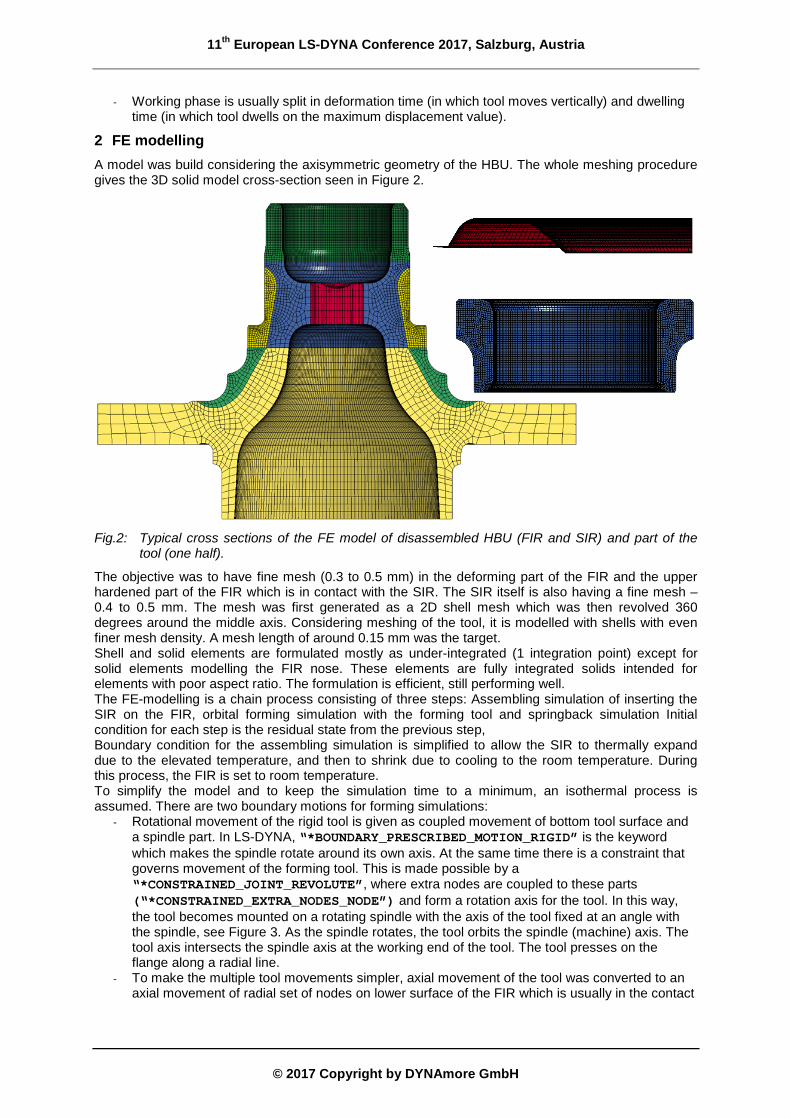
2 FE modelling A model was build considering the axisymmetric geometry of the HBU. The whole meshing procedure gives the 3D solid model cross-section seen in Figure 2.
Fig.2: Typical cross sections of the FE model of disassembled HBU (FIR and SIR) and part of the
tool (one half).
The objective was to have fine mesh (0.3 to 0.5 mm) in the deforming part of the FIR and the upper hardened part of the FIR which is in contact with the SIR. The SIR itself is also having a fine mesh – 0.4 to 0.5 mm. The mesh was first generated as a 2D shell mesh which was then revolved 360 degrees around the middle axis. Considering meshing of the tool, it is modelled with shells with even finer mesh density. A mesh length of around 0.15 mm was the target. Shell and solid elements are formulated mostly as under-integrated (1 integration point) except for solid elements modelling the FIR nose. These elements are fully integrated solids intended for elements with poor aspect ratio. The formulation is efficient, still performing well. The FE-modelling is a chain process consisting of three steps: Assembling simulation of inserting the SIR on the FIR, orbital forming simulation with the forming tool and springback simulation Initial condition for each step is the residual state from the previous step, Boundary condition for the assembling simulation is simplified to allow the SIR to thermally expand due to the elevated temperature, and then to shrink due to cooling to the room temperature. During this process, the FIR is set to room temperature. To simplify the model and to keep the simulation time to a minimum, an isothermal process is assumed. There are two boundary motions for forming simulations:
- Rotational movement of the rigid tool is given as coupled movement of bottom tool surface and a spindle part. In LS-DYNA, “*BOUNDARY_PRESCRIBED_MOTION_RIGID” is the keyword which makes the spindle rotate around its own axis. At the same time there is a constraint that governs movement of the forming tool. This is made possible by a “*CONSTRAINED_JOINT_REVOLUTE”, where extra nodes are coupled to these parts (“*CONSTRAINED_EXTRA_NODES_NODE”) and form a rotation axis for the tool. In this way, the tool becomes mounted on a rotating spindle with the axis of the tool fixed at an angle with the spindle, see Figure 3. As the spindle rotates, the tool orbits the spindle (machine) axis. The tool axis intersects the spindle axis at the working end of the tool. The tool presses on the flange along a radial line.
- To make the multiple tool movements simpler, axial movement of the tool was converted to an axial movement of radial set of nodes on lower surface of the FIR which is usually in the contact
11th European LS-DYNA Conference 2017, Salzburg, Austria
with the fixture. “*BOUNDARY_PRESCRIBED_MOTION_SET” is the LS-DYNA keyword for the node set movements.
Fig.3: The revolute joint principle: In a general application (left), and in the orbital forming application.
In order to compensate for stiffness of the machine head, a linear spring has been added to the spindle. The upper end of the spring has all degrees of freedom locked, while the lower end may move in the axial direction, followed by the spindle movement. An experimental attempt was made to measure this stiffness. Unfortunately, the load cell of the applied device was limited to cope with a non-linear stiffness response. To overcome this, the FE-model was instead calibrated to the global response with a linear spring stiffness. Keyword “*CONTACT_FORMING_SURFACE_TO_SURFACE_SMOOTH” was used for contacts between
- the tool and the deformed flange (nose), and - the nose and the small inner ring.
This is a contact for metal forming applications, where a smooth curve-fitted surface is used to represent the master segment, so that it can provide a more accurate representation of the actual surface, reduce the contact noise, and produce smoother results with coarse mesh. Orientation of the tool mesh (all normals) must be in the same direction. In all other contacts throughout the model, “*CONTACT_AUTOMATIC_SURFACE_TO_SURFACE” was used.
2.1 Material The upper part of the FIR is profoundly deformed under the forming process. Therefore, it is very important to have good data for those large plasticity levels. Compressive testing generates material curves for plastic deformation in plain strain of up to 80 %. To have values beyond the tested ones, the curves were extrapolated to 100 % plastic straining and then the constant value was assumed to 200 % plasticity, see Figure 4. The material response is temperature and strain rate dependent. To simplify the simulations, the process is assumed to be isothermal and strain rate independent since the raised forming temperature introduces material softening that offsets the influence of strain rate hardening.
11th European LS-DYNA Conference 2017, Salzburg, Austria
Fig.4: Compression material data for three strain rates and two temperatures: room temperature and
80 degrees Celsius.
During the calibration study, it was obvious that the isotropic tabulated model (MAT 24 in LS-DYNA) based on the experimental stress-strain hardening curves in Figure 4, gave higher forming force than measured. In order to lower the forming force, the material model MAT 103 was applied. This visco-plastic material model with possibility to define either kinematic hardening or a combination of kinematic and isotropic hardening gave a reduction in the simulated forming force and a well corresponding shape of the formed flange profile. In order to optimize the hardening parameters simple material test in the computational environment has been made. One element model was exposed to a cyclic tension/compression load. The calibration was an optimization problem, where the objective function was to minimize difference between response obtained with the tabulated tension/compression experimental data, blue/black curves, and response obtained with data for the MAT 103 model, green/red curves in Figure 5. The objective curve is actually a combination of tabulated material models for tension and compression – in the first cycle following the tension curve, otherwise following the compression one.
Fig.5: The material response of a cyclic simulation where the tabulated tension (artificial) and
compression material data, blue/black curves is compared to two mixed hardening models (two different set-ups of MAT 103 model) given by green/red curves.
11th European LS-DYNA Conference 2017, Salzburg, Austria
Two optimization processes gave two different set ups for mixed hardening model, with the difference that the green curve gave better agreement with the orbital forming experiments.
3 Results For correlation of the model, two bearings without outer ring and balls were rolled in the calibration phase, while eight bearings were rolled in the validation phase. This is done to confirm that the model is representing the real process with different part geometries and wide ranges in process parameters. Once the calibration work had showed good agreement between experiments and simulations, the validation study was performed, also with a good correlation. The result overview of the work can be found in Figure 6 to Figure 10 in the form of rolled profiles’ comparison. To accomplish the correct height after rolling, the axial movement of the orbital forming tool had to be increased for some FE models in the validation phase. The reason behind the discrepancy between model and experiments is a measurement uncertainty in the axial tool movement. Partly, the recorded machine head movement is not representing absolute movement of the tool. Furthermore, the whole machine head is an assembly of different parts with relative movements in between them so that the machine head acts as a spring whose stiffness changes with different tool set-ups.
Fig.6: Cut profiles from two calibration experiments vs FE-simulation contours (green curves): Calibration case with minimum load (left) and Calibration case with maximum load (right).
Fig.7: Cut profiles from validation studies 1-1 and 1-2: experiments vs FE-simulation contours (green curves).
11th European LS-DYNA Conference 2017, Salzburg, Austria
Fig.10: Cut profiles from validation studies 4-1 and 4-2: experiments vs FE-simulation contours (green
curves)
4 Summary and conclusions The purpose of this work was to develop a finite element model of the orbital forming process performed on a reduced HBU3 assembly without outer ring and balls. This included a calibration study with a following validation of a series of orbital forming processes where geometry and process parameters were varied. To achieve reasonable computational times with good agreement between simulation and experimental results, the following measures were taken.
1. As a base, material data from compression tests were used. To decrease the simulation time, the process was considered isothermal using a mixed hardening model without strain rate dependency.
2. A discrepancy between the model and measured axial movement of the tool was found. The measuring device on the machine gave values which do not represent the absolute movement of the tool. Additionally, the machine head containing the exchangeable tool have a non-linear stiffness behavior during loading. In the model, the machine behavior is represented by a spring having linear properties. Consequently, the model could not be calibrated giving accurate simulations using the axial tool movement. Instead, the final height of the formed nose was found to be the most important calibration parameter.
The validation study confirmed good agreement between the FE simulations and experiments. The model can predict final shape, needed orbital force, residual stress level in the flange and displacement of the raceway in the bearing. Generally, it gives a good input to verify design of orbital forming processes.
5 Literature [1] J Hallquist: " LS-DYNA KEYWORD USER'S MANUAL", February 2013