7 -Ai84 124 AN INTERACTIVE ORGANIZATIONAL CHOICE PROCESSING SYSTEM
I/1TO SUPPORT DECISIO (U) NAVAL POSTGRADUATE SCHOOLMONTEREY CA S N KANG JUN 87
UNCLASSIFIED F/G 5/1 UL
E///EE//EE/I/EEIIIIIEEEEIIIEEI//II///////IEIIIIIEEEEEEEEI//EE////EEEEIE/////EEEEEE/
111 ' I~1113.2 2.2111112.
J.8-
1111.25 III .4 1. 6
MICROCOPY RESOLUTION TEST CHARTNATIONAL BUJREAU OF STANOARDS 1963-A
N, * ~ ~ U S ~ ~ --
.0 w .
q~A.0
N NAVAL POSTGRADUATE SCHOOLMonterey, California
DTICSELECTE
SEP 0 4 1987
THESISAN INTERACTIVE ORGANIZATIONAL CHOICE
PROCESSING SYSTEMTO SUPPORT DECISION MAKING BY USING
A PRESCRIPTIVE GARBAGE CAN MODEL
by
Kang, Sun Mo
June 1987
Thesis Advisor Taracad R. Sivasankaran
Approved for public release; distribution is unlimited.
-,87 9 1 313
unclassifiedSECLRtry CLASS41CATION OF THIS PAGE
REPORT DOCUMENTATION PAGE
'a REPORT SECURITY CLASSIFICATION 1b RESTRICTIVE MARKINGS
unclassified2a SECLR'TY CLASSIFICATION AUTHORITY I OISTRIBUTION'/AVAILABILITY OF REPORT
Approved for public release;2b DECASSFCATON DOWNGRADING SCHEDULE distribution is unlimited.
4 PERFORMNG ORGANIZATION REPORT NjMBER(S) S MONITOkiNG ORGANIZATION REPORT NuMBER(S)
6a NAME OF PERFORMING ORGANIZATION 6t OFFICE SYMBOL 7a NAME OF MONITORING ORGANIZATION
Naval Postgraduate School (IfdopliCable) Naval Postgraduate SchoolI2
& ADDRESS City, State, and ZIPCodfe) 7b ADDRESS (City. Stare, and ZIP Code)
Monterey, California 93943-5000 Monterey, California 93943-5000
Ba NAME OF FUNDING, SPONSORING 8b OFFICE SYMBOL 9 PROCUREMENT INSTRUMENT IDENTFICATION NUMBERORGANiZATiON (If applicable)
*" c aDDRESS(Ciry. State. ard ZIPCode) 10 SOURCE OF FUNDING NUMBERS
PROGRAM PROJECT TASK WORK JNITELEMENT NO NO NO ACCESS:ON NO
( Include Secu y Clasificaion)AN INTERACTIVE ORGANIZATIONAL CHOICE PROCESSING SYSTEM
TO SUPPORT DECISION MAKING BY USING A PRESCRIPTIVE GARBAGE CAN MODEL
" ,ERSONA, AuTOR(s) Kang, Sun Mo
M 1 s e sis 3tME COVERED 14 1 ET7OfJMOT,, (Year,. Month Day) 15 PAGE (ODNT 92
'6 SLP - "'%iM %N ARY NOTATION
COSAT CODES 18 SUBjECT TERMS (Continue on reverse if neceisary and identfy by block number)
7:: GROUP SUB.GROUP prescriptive garbage can model; organizationalchoice processing system
I AB'SRAC' (Continue on reve;e if necessary and identify by bloca number)
*This thesis discusses and implements an interactive decision support sys-tem using a Prescriptive Garbage Can Model. The fundamental presumptionis that if the choice-outcome relationships in an organization can beobserved and evaluated, it is possible to extract predictiveness fromuncertain streams, and allow the organization to shift to a less randomstrategy. Solving organizational problems consists of selecting thosechoices that lead the organization in a direction towards the ideal state.Thus, it is convenient to model the organizational state transitions asa Markovian process with stationary properties. The purpose of a Pres-criptive Garbage Can Model is to advise the participants of the choices
* available in a current situation, and to present choice policies leadingthe highest potential benefits. Also a method of interfacing the currentsystem with an expert system for intelligent decision making is examined.
,0 D S ' 3j' ON, AVAILABILITY OF ABSTRACT 21 ABSTRACT SECURITY CLASSIFICATION
El .%CLASSIF'ED.,NL:MITED 0 SAME AS RPT r-OTIC ,SERS unclassifieditUa N.A E OF RESPONSIBLE ,DIViDUAL 22b TELEPHONE (Include AreaCode) 22c OFf,( Si'MBiX
' Prof. Taracad R. Sivasankaran (408) 646-2637 Code S4SD FORM 1473, 84 MAR 83 APR ed,t,on may be used untaexhau ted SECURITY CLASSIFCATON OF ',S PACE
All other edoton ar obolete unclassified
Approved for public release; distribution is unlimited.
An Interactive Organizational Choice Processing Systemto support Decision Making by usingA Prescriptive Garbage Can Model
by
Kang, Sun MoMajor, Korean Army
B.S., Korean Military Academy, 1979
Submitted in partial fulfillment of therequirements for the degree of
MASTER OF SCIENCE IN COMPUTER SCIENCE
from the
NAVAL POSTGRADUATE SCHOOLJune 1987
Author: /$ C I-')Kang, Sun Mo
Approved by:Taracad R. Sivasankara Thesis Advisor
C ..D ary S. Baie-r' Seco- d Reader .
•
4
Departmey of Computer Science
Kneale T. MarsDean of Information and PolcyScier 6'-
ABSTRACT
This thesis discusses and implements an interactive decision support system using
. a Prescriptive Garbage Can Model. The fundamental presumtion is that if the choice-- outcome relationships in an organization can be observed and evaluated, it is possible
to extract predictiveness from uncertain streams, and allow the organization to shift to
a less random strategy. Solving organizational problems consists of selecting those
choices that lead the organization in a direction towards the ideal state. Thus, it is
convenient to model the organizational state transitions as a Markovian process with
stationary properties. The purpose of a Prescriptive Garbage Can Model is to advise
the participants of the choices available in a current situation, and to present choice
policies leading the highest potential benefits. Also a method of interfacing the current
system with an expert system for intelligent decision making is examined.
j I"ei,.h . I. LJ I. , LJ
-A-," __"___
.... ", .7 -- "- ... ......
i'
3
TABLE OF CONTENTS
IN TRO D UCTION .............................................. 8
II. BACKG RO UN D .............................................. 10
A. A STOCHASTIC APPROACH TO THE PRESCRIPTIVEGARBAGE CAN MODEL ................................. 10
B. DEFINITIONS AND ASSUMPTIONS ....................... 11
1. Organizational Elem ents ................................ II
2. Organizational States ................................... 11
3. C h oices .............................................. 11
4. Choice Policies ........................................ 12C. A PRESCRIPTIVE MODEL OF ORGANIZATIONAL
C H O IC E ................................................ 12
1. Organizational Flux as Stochastic Transitions ............... 12
2. Goodness Measure of an Organizational State .............. 16
3. Transition Benefit ..................................... 17
4. Identification of a Choice Policy .......................... 17
5. Reinforcement of Choice Policies throughLearning,' R evision ..................................... IS
III. SOFTWARE DESIGN AND IMPLEMENTATION ................. 19
A. DECISION MAKING PROCESS ........................... 19
1. Intelligence Phase ..................................... 192. D esign Phase ......................................... 19
3. C hoice Phase ......................................... 20
B. DESIGNING THE PGCM HIERARCHY AND DFD .......... 20
1. Hierarchical Program Structure .......................... 20
2. D ata Flow D iagram .................................... 20
C. PGCM PROCESS ALGORITHM ........................... 24
1. Input D ata via Terminal ................................ 24
2. Generate Transition/Benefit Probability(formula 2.1,3,4) ...... 24
4
.
3. Value Determination Operation .......................... 24
4. Policy Improvement .................................... 24
5. Combined Operation in An Iteration Cycle ................. 24
D. IMPLEMENTATION WITH OFFENSIVE OPERATIONEX A M PLE .............................................. 25
1. U ser Interaction ....................................... 26
2. Transition Probability M atrix ............................ 29
3. G oodness M easure ..................................... 29
4. Transition Benefit M atrix ............................... 29
5. Generate the long run choice policy ....................... 31
IV. FURTHER RECOMMENDED STUDIES ......................... 35
APPENDIX A: A SOURCE PROGRAM ................................ 37
APPENDIX B: USER MANUAL .. .................................. 58
APPENDIX C: OFFENSIVE OPERATION EXAMPLE .................... 61
APPENDIX D: UNIVERSITY SCHEDULE EXAMPLE ................... 75
LIST OF REFEREN CES ................................................ 89
INITIAL DISTRIBUTION LIST ......................................... 90
5
LIST OF TABLES
1. AN EXAMPLE ORGANIZATIONAL STATE ......................... 14
2. AN EXAMPLE GOODNESS MEASUREMENT ........................ 16
3. DESCRIPTION OF PROBLEMS AND ORGANIZATIONALST A T E S .......................................................... 27
4. TRANSITION PROBABILITIES IN Z1 . . . . . . . . . . . . . . 30
5. EVALUATING GOODNESS MEASURES ............................ 31
6. TRANSITION BENEFIT MATRIX OF ALL CHOICES ................. 31
7. SELECTED CHOICE POLICIES ..................................... 34
6
"* ,. S.. .. . . 5 .. . . . .
LIST OF FIGURES
2.1 An Example Transition Probability Matrix ............................ 153.1 Hierarchical Program Structure for PGCM ............................ 213.2 Data Flow Diagram for PGCM ..................................... 223.3 System Flow Chart of PGCM ...................................... 25
:N7
!21
p
I -
I. INTRODUCTION
The Prescriptive Garbage Can Model (PGCM) of organizational decision-making
tRefs. 1,2] can be defined as chance events resulting from the interactions of fourelements in the organizational context, (i) problems, (ii) solutions, (iii) participants, and
(iv) choice opportunities. As with every anarchic and random system, the participants
desire to solve the current problem in the most effective manner. Which problems areactually taken up for action, in what priority, what choices are made in solving them.
and how conclusively they are solved, are all functions of ambiguous preferences, andtime and energy constraints of the participants.
A model imparting some degree of structure and comprehensibility to thecomplex organizational interactions and suggesting rational choice policies in an
otherwise irrational context may be of invaluable assistance to organizational decision-
makers. Thus, the model is prescriptive in nature. The building of such a model would
link rational decision-making [Refs. 1,31 with anarchic decision-making [Ref. 2]
thought.
Three objectives of the model are the following
I. Advise the participants of the choices available to them in a specificorganizational state
2. Estimate the expected benefit resulting from each choice
3. Lay down choice policies which would assist the participants in leading theorganization in the long run to the state that has the highest potential benefits
Under severe lack of knowledge, decision makers may adopt a random search andchoice rule, i.e., decisions are ill-defined, inconsistent, unclear, uncertain and
problematic. Learning and outcomes are a matter of accidental trial-and-error.
While random strategies are always available, one may wonder whether they can
-be imbued with conscious thought processes to deal with uncertainty more effectively.
If the choice-outcome relationships in an organization can be observed and evaluated,
it is conceivable to extract predictiveness from uncertain streams, and thereby allow the
organization to shift to a less uncertain strategy, in particular toward cybernetic and
stochastic decision procedures.
This study discusses the design and implementation of the Prescriptive Garbage
Can Model to provide a best course of actions on the anarchic organizational system.
&A-f
Chapter II provides background on the prescriptive organizational model of garbage
can choice policies. This includes a stochastic approach to the garbage can model,
definitions and assumptions about the components of PGCM, and a prescriptive model
of organizational choice. Chapter III examines the decision making process and
discusses the design and implementation using a military offensive operation example.
Chapter IV contains recommendations for further study on the topic. Appendix A isthe source program. Appendix B is the user manual for the current implementation.
Appendix C is a demonstration how offensive operation decision choices could be
taken. Appendix D is a demonstration how university schedule decision choices could
be taken.
V9
-Aj,
'V
'V. - . ' - -:' -. : . ' " " ' "'-".. i -", -". - ' : .": "- . : "'':. '''' .-
1I. BACKGROUND
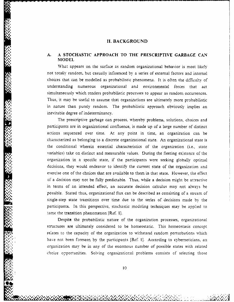
4,' A. A STOCHASTIC APPROACH TO THE PRESCRIPTIVE GARBAGE CANMODEL
What appears on the surface as random organizational behavior is most likely
not totaliy random, but casually influenced by a series of external factors and internal
choices that can be modelled as probabilistic phenomena. It is often the difficulty of
understanding numerous organizational and environmental forces that act
simultaneously which renders probabilistic processes to appear as random occurrences.
Thus, it may be useful to assume that organizations are ultimately more probabilistic
in nature than purely random. The probabilistic approach obviously implies an
inevitable degree of indeterminancy.
The prescriptive garbage can process, whereby problems, solutions, choices and
participants are in organizational confluence, is made up of a large number of distinct
actions sequenced over time. At any point in time, an organization can becharacterized as belonging to a discrete organizational state. An organizational state is
the conditional wherein essential characteristics of the organization (i.e., statevariables) take on distinct and measurable values. During the fleeting existence of the
*. organization in a specific state, if the participants were seeking globally optimaldecisions, they would endeavor to identify the current state of the organization and
exercise one of the choices that are available to them in that state. However, the effect
of a decision may not be fully predictable. Thus, while a decision might be attractive
., in terms of an intended effect, an accurate decision calculus may not always be
possible. Stated thus, organizational flux can be described as consisting of a stream of
single-step state transitions over time due to the series of decisions made by the
participants. In this perspective, stochastic modeling techniques may be applied totame the transition phenomenon [Ref. 1.
Despite the probabilistic nature of the organization processes, organizational
structures are ultimately considered to be homeostatic. This homeostasis concept
relates to the capacity of the organization to withstand random perturbations which
have not been foreseen by the participants [Ref I]. According to cyberneticians, an
organization may be in any of the enormous number of possible states with related
choice opportunities. Solving organizational problems consists of selecting those
10
0% choices that lead the organization in a direction towards the ideal state. Thus, it is
convenient to model the organizational state transitions as a Markovian process with
N stationary properties. A process is stationary when organizational states become stable
and invariant under time shifts. The homeostatic nature of the organizations implies
the operation of at least some stationary properties.
B. DEFINITIONS AND ASSUMPTIONS
1. Organizational Elements
As defined in the PGCM, any organization consists of four relatively
independent elements. They are (i) problems, (ii) solutions, (iii) participants, and (iv)
choices. Relative independence implies that each element can assume its own identity,
existence and relevance. In addition, we presume that problems are triggered by
external or internal factors and represent the mismatch between the current
organizational state and the desired state. Solutions are either tools or answers directly
available within the organization waiting to be bound to the appropriate problems.
Participants with their limited stocks of energy focus their attention on important
problems and search for attractive solutions. Choices act as a cementing factor that
ties the above three elements together.
2. Organizational States
The organizational state Zi is a function of three attributes which describe an
organization at a certain point in time. These attributes are:
I . The importance of the problems remaining to be solved (Pi)'
2. The effectiveness of the solutions applied to problems (Si) in the recent past.
7. The energy levels of the participants available for problem-solving (El).
The choice of P, S and E as attributes of organizational states is motivated by
the structure of the PGCM which employs these elements as building blocks. P, S and
E are assumed to be independent and measurable attributes. For convenience of
representation, we shall use the coordinate system to denote a state. Thus an
organizational state, Zi = f Si, E.
3. Choices
Choices are decisions taken by participants in their pursuit to solve problems.
They are determined by judging the nature of problems remaining to be solved, the
'effectiveness of the considered solutions, and the energy input available from the
(11
dj
................ -
participants required of a particular choice. In an organized anarchy, choices are
.2 iassumed to be made accidentally. However, if choices were to be made rationally
amidst the anarchy, they would presumably carry the organization towards the state
(0,1,1). Rational managers would prefer such a state because they would like to see as
many of the remaining important problems solved as possible. in an effective manner,
and have at their disposal at all times a adequate supply of energy that can be applied
to future problem solving. This is not to imply that managers wish to remain absorbed
in state (0,1,1), since this means no opportunities, eternal calculations and unexpended
energy. Rather, managers would prefer to attain a dynamic equilibrium at or close to
(0,1.1). At such equilibrium, there is a continuous flow of problem opportunities and
their effective resolution in a timely fashion so that sufficient manpower energy is
readily available to meet new problem opportunities as soon as they arise.
In general, selecting a choice induces the transition of the organization to a
new state in the next time interval. It is possible that taking no decisions is a choice in
itself. It can shift the current state to a new state with more problems.
4. Choice Policies
Choice policies provide a prescriptive approach to problem solving. Once a
set of organizational states and associated choices available therein can be identified, itis possible to bring to bear rationality in decision-making by laying down choice
policies. Choice policies consist of suggestions as to what choices should be preffered
- whie the orcanization is perceived to be in a particular state. In a sense, choice
policies form a set of guidelines for organizational decision makers. Usually, the choice
policies are so recommended as will most likely bring in the maximum benefits for the
organization in the long run.
C. A PRESCRIPTIVE MODEL OF ORGANIZATIONAL CHOICE
S1. Organizational Flux as Stochastic Transitions
Introducing rationality into an anarchic system requires that the decision-
makers observe a calculus of outcomes based upon the (i) understanding of the
implications of the various organizational states, (ii) knowledge of all the choices
available to them in each state, and (iii) assessment of the probable impact of
exercising a choice on the current state, before they reach a decision. We infuse
rationalitv into the Prescriptive Garbage Can Model of anarchic actions through the
use of a transition probability matrix.
12
<- .
~w IIq!Im ,I _ y..u,, .qI,,, ..Ircr i : ; II ..L , ,- - 4, -, -. . -;. , - '.7 _w rz . 2, .7 W . 'r -* - - J . . . .
The transition probability matrix represents the various organizational states,
the available choices under each state, and the probabilities with which a choice cantake the organization from one state to another. Z , i = I .... , n, denotes the
organizational states; Ci (k), k = 1 .... , m i , the choices available in a state i; qI
.. F c(k). the probability that the initial state Zi will transit to Z when some choice Ci (k)
F:,:-- is taken. Implicit in the matrix is the fact that there is no guarantee a choice canalwavs lead to a state that is predictable beforehand. Impossible states may be filtered
out Irom the matrix altogether and infeasible transitions may be represented by zeros.
Note that qjqij c- (k) = 1. For simplicity of notation, we omit the subscript i in ci (k),and denote by c(k).
The prescriptive model requires the determination of the transition
probabilities. While several methods have appeared in the literature in estimating
subjective probabilities, one that has evoked considerable interest in recent years
consists of systematic elicitation of expert judgement [Refs. 1,4,51. Expert knowledge
and opinions often form an adequate surrogate, when historical data seem either
inapplicable or unavailable.
The following steps describe the mechanics of generating the transitionprobability matrix
Step I . Determination of the set of organizational states, n.
First, determine the number of possible values p can take. For this divide the
scale (0,1) into as many scale points as possible, say r. Assuming these scale points are
uniformly distributed, the value of each scale point p can be generated using the
formula,pu = (u-) ' (r-l), where u = I ,.., r.
For example, if r= 3, then p1 _ 0, p" = 0.5, = 1. The same formula can beapplied to determine the scale points for S and E. The value of r need not have the
same value for P, S, and E.
Second, generate all possible combinations of pU , Su , Eu to determine all
organizational states. If r= 2 for P, S and E, then the different organizational states
can be described by one of the combinations, (Pl, S1, El), (P1. S1 , E2 ), (Pl. S2 , El),,P1 S21. E2), (p2 ', l, E)9 (P 2, Sl, ), (p 2. S2, El), and (p 2, S2, E2). In general.
assuming the partitions are equal for P, S and E (rp = rs = re) the maximum number
of possible organizational states that can be represented using the (P,S,E) coordinate
13
'-N
form is thus r3 . If r= 2, these states can be denoted by Zi = (Pi, Si, Ei) where i = I,.,8. Thus, Z I=(PI, SI , E'), Z2--(PI, S1, E2), ..., Z8=(P2, S2, E2)
Note that once each possible combination (pU, Su, Eu) is assigned to a specific state
Z i, i= 1,...,n, the actual values of P, S, E's in any state thereafter be refered to by Pi, Si
and Ei. The following Table I represents each organizational states.
TABLE I
AN EXAMPLE ORGANIZATIONAL STATE
State Zi (Pi , Si , Ej) Remarks
1 (0.0,0.0,0.0)2 (0.0,0.0,1.0)3 (0.0,1.0,0.0)4 (0.0,1.0,1.0)5 (1.0,0.0,0.0)6 (1.0,0.0,1.0)7 (1.0,1.0,0.0)8 (1.0,1.0,1.0)
* Step 2 : For each of the states Z i , identify and filter all the conceivable andfeasible choices.
Collect all these choices to form a set defined by Di = k c(k), where k = 1,
mi. In complex organizations, exhaustive enumeration of choices may be a difficult
task. However, it is not unrealistic for organizations to anticipate and equip
themselves with as many available choices as they can to meet different possible
situations.
Step 3 : For an initial state Z i , pick one of available choices
As a result of c(k), assume the organization enters state Z:.
* Step 4 : Estimate the probabilities P, S, E
-Bpi , c(k), where j = 1 ... , n and 7j -pi pj c(k) = 1. Repeat for elements
S and E. This gives jpi 'p c(k) , and Epi , pj c(k).
14
*.Step 5 : Compute the row of the transition probability matr-ix using thefollowing formula
qjj c(k) = pi, Pjc(k) * Si, j k)* 9p , pjc(k) (eqn 2. 1)
herein, we notated P- , S , E as estimation probabilities of P, S, E
0Step 6: Repeat for all remaining (mi - 1) choices in 4i.
0 Step 7: Repeat steps 3-6 for the remaining (n -i) states.
The general layout of the transition probability matrix is shown Figure 2.1.
Next State
u Z1; C(ml) qllC(ml) ql2C(ml) ql3C(ml) . qlnC(ml)rr Z2 Cl q2lC( 1) q22Cl q23Cl ... q2nC(l)
e Z2' C() 2JC 2) q22C(2) q23C(2) . .. q2nC(2)n..t Z2,;C(m2) q2lC(m2) q22C(m2) q23C(m2) .. q2nC(m2)
S Z3, C(1) q3lC( 1) q32C(1) q33C(1) .. q3nC(1t Z3, C(2) q3lC( 2) q32C(2) q33C2) ... q3nC(2)a..t
*e Z3, Ck m3) 4.?lC(m3) q32C(m3) q33C(m3) q3nC(m3)
Zn, C(mi) qnlC(mi) qn2C(mi) qn3C(mi) ... qnnC(mi)
Number of states = Z(1,., n);
Number of choices in each state = C(l,., mi);
TLransition probability matrix satisfies the condition
-j qi C( k) = 1, for k = 1, ...
A Figure 2. 1 An Example Transition Probability Matrix.
15
-r VOL~&4 'Uk
2. Goodness Measure of an Organizational State
For each organizational state Zi , we assume there is an associated measure of
goodness, gi" This measure is ordinal in nature and reflects the amount of benefit
derivable from the values of P, S and E corresponding to each state. The idea is
similar to a balance sheet which conveys the state of health of an organization. S and
E can be viewed as assets in a balance sheet, since they represent the strength of the
organization. On the other hand, P can be viewed as a liability in that it detracts from
the organizational performance. Note that high values of Si and Ei imply high values
of gi' Conversely, high values of Pi imply low values of gi" The composite amount of
goodness for the state Zi can be expressed as follows
gi =- Pi + Si + Ei (eqn 2.2)
In theory, the ideal state of the organization corresponds to g = 2, since P -
0, S = 1, and E = I. Contrarily, for the anti-ideal state, g = -1, since P = ,S 0
and E = 0. The following Table 2 shows each goodness measurement.
TABLE 2
AN EXAMPLE GOODNESS MEASUREMENT.,
State Zi (Pi ' Si I Ei) Goodness Remarks
1 (0.0,0.0,0.0) 0.02 (0.0,0.0,1.0) 1.03 (0.0,1.0,0.0) 1.04 (0.0,1.0,1.0) 2.05 ( 1.0,0.0,0.0) -1.06 (1.0,0.0,1.0) 0.07 (1.0,1.0,0.0) 0.08 (1.0,1.0,1.0) 1.0
16
N N
3. Transition Benefit
The goodness measure of an organizational state can be related to the
transition probabilities through the idea of transition benefit. Transition benefit is the
expected incremental goodness due to a transition that results from a specific choice.
It is calculated as follows.
Step I : Difference of goodness value between current state Zi and terminalstate Zj for choice c(k)
(gj - gi)c(k) = - (Pic(k) - Pi) + (Sjc(k) - Si) + (Ejc(k) - El) (eqn 2.3)
Step 2 : Expected incremental benefit (G) of the choice
G (Zi , c(k)) = Ej (gj - gi)c(k) * qijc(k) (eqn 2.4)
If there are n states and i mi choices, the transition benefit matrix will be
dimension of n x Y, mi.
4. Identification of a Choice Policy
We have seen that policy is a prescriptive function. Its purpose is to suggest
which choice c(k) out of the possible set of choices c(1,2, ... ni) must be acted upon,
given the organization is in state Zi If rationality in decision making is assumed,
choices will have to be so exercised as to maximize gi" This can be achieved by
maximizing the sum of the expected selection and sequencing of the different choices.
Howard's algorithm can be employed to perform the maximization [Refs. 6,7]. The
algorithm is applicable while dealing with a stochastic process where the law of
transition and the corresponding benefit function are known. It consists of an
intelligent trial and error iterative procedure that selects the best beneficial choice for
each state in each iteration until the long run expected mean income per choice is
maximized. The following one is the dynamic programming formulation.
* F V(S) max(i(S,a) - g + Y v(s)q S . s C(a)}, for s = 1, .. S (eqn 2.5)
'81
17
-3
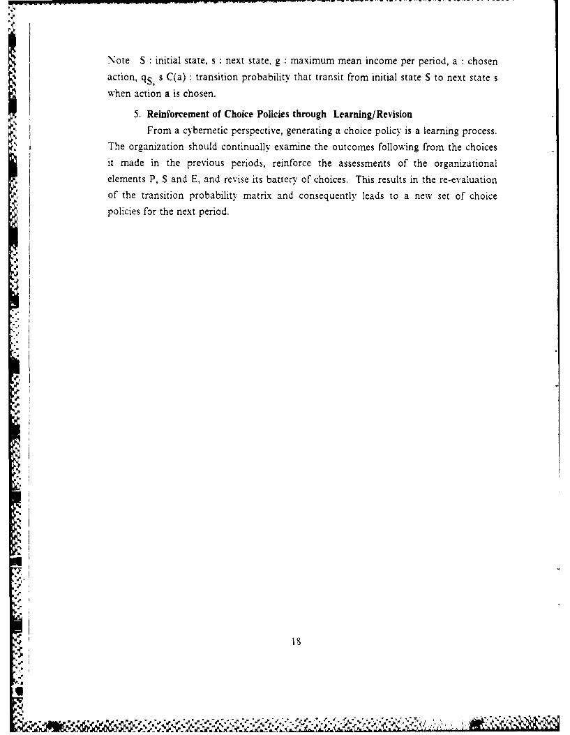
Note S : initial state, s : next state, g : maximum mean income per period, a : chosen
action, qs, s C(a) : transition probability that transit from initial state S to next state s
when action a is chosen.
5. Reinforcement of Choice Policies through Learning/RevisionFrom a cybernetic perspective, generating a choice policy is a learning process.
The organization should continually examine the outcomes following from the choicesit made in the previous periods, reinforce the assessments of the organizationalelements P, S and E, and revise its battery of choices. This results in the re-evaluationof the transition probability matrix and consequently leads to a new set of choice
policies for the next period.
1'%
I'
4..
,Is
III. SOFTWARE DESIGN AND IMPLEMENTATION
A. DECISION MAKING PROCESS
The Prescriptive Garbage Can Model refers to a class of systems which supportthe process of making decisions. The decision maker can retrieve data and testalternative solutions during the process of problem solving. This system also should
provide ease of access to the data base containing relevant data and interactive testing
of solutions. The system analyst must understand the process of decision making for
each situation in order to analysis a system to support it. The model proposed by
Herbert A. Simon consists of three major phases [Ref. 91, they are (i) intelligence
phase, (ii) design phase, and (iii) choice phase.
1. Intelligence Phase
Searching the environment state calling for decisions. Estimation data are
obtained, and examined for clues that may identify problems; set all estimationprobabilities. One of the important fact is how to formulate the problems. A problem
formulation might have a risk of solving the wrong problem, but the purpose of
problem formulation is to clarify the problem so that design and choice activities
operate on the right problem [Ref. 9]. Frequently, the process of clearly starting the
problem is sufficient; in other cases, some reduction of complexity is needed. Four
strategies for reducing complexity and formulating a manageable problem are [Ref. 9]
*. Determining the boundaries
*. Examining changes that may have precipitated the problem
*. Factoring the problem into smaller subproblems
*. Focusing on the controllable elements
A Prescriptive Garbage Can Model can obtain intelligence through searching,
hence allow the user to approach the task heuristically through trial and error rather
than by preestablished, fixed logical steps. So establishing analogy or relationship to
some previously solved problem or class of problems is useful.
2. Design Phase
Inventing, developing, and analyzing possible courses of choices is performed
in this phase. It involves processes to understand the problem, to generate solutions
and to test solutions for feasibility. "A significant part of decision making is the
19
.4
generation of alternatives to be considered in the choice phase" [Ref. 101. The act of
generating alternative is creativity that may be enhanced by alternative generation
procedures and support mechanisms. In this process, an adequate knowledge of the
problem area and its domain knowledge, and motivation to solve the problem will be
required. Given these situations, analogies, brainstorming, checklists can enhance
these creativities [Ref. 9].
3. Choice Phase
Selecting an choice from those available by using decision making
software(.i.e., PGCM), can establish all choices for each organizational state.
B. DESIGNING THE PGCM HIERARCHY AND DFD
1. Hierarchical Program Structure
To process the PGCM, we first set up estimation probabilities and alternative
actions through intelligence,' design phase. Then we also establish choice policiesthrough choice phase. Herein we focus on the choice phase that consists of two
procedures. One is to produce all matrices such as organizational states, transition
matrix, goodness measure table, benefit matrix from given userrequirements, specification. The other one is to apply these matrices to generate longrun policy. Figure 3.1 shows the modules that are invoked by the main PGCM
program. As we see, each of modules is a black box that takes input data, performs
some transformation on that data, and process output data.
2. Data Flow Diagram
Since we are establishing modules as functional elements, we need to knowwhat are the inputs,'outputs. So for each module we will use a simple black box
diagram to show the data flow of PGCM. For example, in Figure 3.2, there is amodule labeled benefit matrix. Independent of all other modules in the program, we
need transition matrix and goodness measure table. The followings are the
inputs outputs parameters for each module [Ref. Il].
Module Getinfo (level 1.1) **
inputs • number of scale points for each factor (rp, rs , re)
number of different choices for each state
estimation probabilities
process: store input data via user interaction
20
N
i} output: estimation probability table
Get ri
GModule Gets (e 1.2) G-info state transi goodness benefittion mat. mat.
Initi- Dynamic Resolve 5etnewalize formula variable action
. . t i o n
Figure 3.1 Hierarchical Program Structure for PGCM.
** Module Getstate (level 1.2) **,'input : number of scale points for each factor (rp, rs ,re)
~process: combinatc all scale points
i output : organizational state table (size : n = r p * r s *re)
! ** Module Gettransition (level L.3))*
inputs : estimation probabilities
organizational state table
21
process: calculate transition probability using formula 2.1
output : transition probability matrices (size : n * ( mi * n))
Policy
p- v
24ue32DtaFo iga 2.2 aG2.1
I1.1
et Module Getoodnew- -eesoeood nt
inu :ogai a ction aate tabiz
F1 sorce/:proess - :dat flodestinations
5.J
~1 f~
Figure 3.2 DaaFo.Darmfo5GM
MUle Getgoodness (level .4)n enfi
process: calculate goodness measure using formula 2.2output : goodness measure table (size : n)
~22
D*1tmto D rnytonr3 eei
Poic
** Module Getbenefit (level 1.5) **
inputs : transition probability matrices
goodness measure table
process: calculate transition benefit probability using formula 2.3, 2.4
output : transition benefit matrix (size : n * maxchoice)
** Module Initialize (level 2.1) **
input : transition benefit matrix
process: select best choices for each state from transition benefit matrix that
has the highest value in that state
output : policy table (size : n)
** Module Dynamicformulation (level 2.2) *
inputs : transition benefit matrix
transition probability matrices
temporary policy table
process: fill the coefficient table need to solve equations described by formula 2.5
output : coefficient table (size : n * n+ 1)
Module Resolvevariable (level 2.3) *
input : coefficient table
process: resolve variable using gaussian elimination method
output : variable values
** Module Setnewaction (level 2.4) **
inputs: variable values
transition benefit matrix
:ransition probability matrices
23
.4
!fv~
process: set a new policy using howard algorithm
output : new policy table
C. PGCM PROCESS ALGORITHM
1. Input Data via Terminal
The current PGCM system needs to know number of scale points for eachfactor, different number of choices, and the estimation probability.
2. Generate Transition/Benefit Probability(formula 2.1,3,4)
3. Value Determination Operationa) establish n linear simultaneous equations (vi , g).
I : use qij and i(S,a) for a given policy to solve
g + vi = i(S,a) + 7 qij vj i = 1,2,..., n
b) set arbitary vi equal to 0, normally vnc) resolve and produce the relative values using gaussian method.
4. Policy Improvementa) find the alternative C(k) that maximizes the test quantity (vi , g).
find max i(S,a) C(k) + qij C(k) vj} using the relative valuesvi of the previous policy, then C(K) becomes the new decision in the
ith state, i(S,a) C(K) becomes i(S,a), and qij C(K) becomes qijb) perform this procedure for every state, and determine a new policy.
5. Combined Operation in An Iteration Cycle
a) select an initial policy from immediate benefit values.
b) solve the relative values vi and g by setting vn to 0.
c) fimd an alternative that has maximal benefit values.
__ d) if all alternatives are equally same benefit values, leave it unchanged
1) sort benefit values (1 .. choice(.n.))
2) calculate absolute difference for each benefit values3) ifa difference is less than 0.0001, take an old action else set
a new action
24
%@
e) repeat until the policies on two successive iterations are identical
f) if gain value g is decreased, then set arbitary vi. 1 equal to 0,
and repeat step3 thru step 5 until satisfied
The above algorithms step 3 thru step 5 based on the policy iteration method
for multiple chain processes (Ref. 61.
D. IMPLEMENTATION WITH OFFENSIVE OPERATION EXAMPLE
Decision making in battle field involves unclear problems, chance event solution-,
fluid energy derived from participants, and choices that seldom resolve problems. At
any moment in time, a battle field may have a large number of problems to dealwith, different possible solutions to cope with these problems, and many participants to
make the necessary choices. Since taking into account all of the problems
simultaneously could confuse the illustration, we shall assume that there is only one
problem to be addressed during the interval of time considered and that the problem is
related to offensive operation. We assume the representative elements in the offensive
operation are number of attack forces, weapon systems, weather, relation to the
consequent military operation. Figure 3.3 shows a system flow chart of thePrescriptive Garbage Can Model process.
Prescriptive Garbage Can Model
Estimation Probability
UserInteraction Transition Prob. Benefit Prob. Result
G7odness Measure
Howard Algorithm
Figure 3.3 System Flow Chart of PGCM.
25
.I4
1. User Interactiona. Define the problem and determine the organizational states
Once we define the problem and number of scale points for each factor, we
can combinate the organizational states. We shall limit the number of scale points to
P = 3 (0, 0.5, 1.0), S = 3 (0, 0.5, 1.0), E = 2 (0, 1.0). Thus, if we take into account
all the combinations of (Pi , Si , E), we can have at most 18(3x3x2) possibleorganizational states. Table 3 shows the description and the organizational states of
this problem.
b. Identify and filter all the conceivable and feasible choices
In this example, we choose only 4 choices towards solving the offensiveoperation problem. They are
C(l): Smoke operation and do attack
C(2) Supporting high performance weapon systems
I C(3) Reinforcing attack forces
C(4) Changing attack forces
I: - For instance, (0.5, 0.5, 1.0) is one of these combinations denoted in our
Fable 3 by Z 10 . It can correspond to a situation where an offensive forces have a
good chance to attain their objectives successfully since they have no significant
problems. But the military expert may have some questions such as the enemy'srecovery ability from the previous shock or friendly forces's risks caused by a little
i shortage of attack forces, etc. So the military expert may look for another action toprotect friendly forces such as a smoke operation. A smoke operation can significantly
reduce the enemy's effectiveness in both the day time and at night. Combined with
suppressive fire, smoke will provide increased opportunities for maneuver forces to
deploy while minimizing losses. Also the effective delivery of smoke at the critical timeand place on the battle field will contribute significantly to the combined arms team
winning the first battle. Therefore, we we choose a smoke operation as one of feasibie
choices. The rest of the choices are also chosen in a same manner. Generally eachstate may have a different set of feasible choices for each state. For example, we can
pick out C(4) since Z6 is an ideal state we don't have to retain on C(4) which can be
selected in the worst situation. so Z6 has 3 choices. Hereby, we bring an interfaceproblem between PGCM and expert system that identify and filter all the conceivable
26
04l- .
TABLE 3
DESCRIPTION OF PROBLEMS AND ORGANIZATIONAL STATES
P; Importance of problems to be solved
S :Degree of effectiveness in problem-solvingE Potential energy of participants
pl=0 No significant problem regarding attack forcesmission load, weather, rela ion with consequenmilitary operation
p2=.5 Moderate shortage of attacking forces, not good,weapon system good weather, a certan ime delayto the consequent operation
p3=1 Acute shortage of attacking forces, biy missionload, bad weather, a tremendous time de ay to theconsequent operation
S1=0 Most of personnel have no experience in the battlefield, poor coordination with adjacent unit,poor per ormance weapon systems
$2=.5 ome personnel have an experience in the battlefield appropriate coordination and reasonableattack-de ~ense forces ratio, good performanceweapon systems, good logistic support systems
S3=1 Some personnel have an experience in the battlefield, excellent coordination, best attack-defenseforces ratio, excellent performance weapon systems
sufficient logistic support systems
E1=0 Not quite proud of their operations,passive actionE2=1 High morale, high responsibility
State Zi (Pi / Si I Ei ) Remarks
i 0.0,0.0,0.03 0.0,0.0,1.0
S3. 0, 0.5,0.04 0.0,0.5,1.05 0.0,1.0,0.06 0.0,1.0,1.0 ideal7 0. 5,0. 0,0. 08 0.5,0.0,1.09 0.50o.5,0.0
10 0.5,0.5,1.0p 1 0.5,1.0,0.0
p ~12 0.5,1.0,1.0 at-da13 1.0,0.0,0.0 anti-ideal14 1.0,0.0,1.015 1. 0,0. 5,0. 016 1.0 0.5,1.017 1.0,11.0,0.0
""18 1.0,1.0,1.0
and feasible choices, if our problem has hundreds of organizational states. That system
certainly helps all experts. For the simplicity, this example has all the same number of
choices for each state, and Appendix D shows a different number of choices for each
staze.
:j 27r. % ' t
I
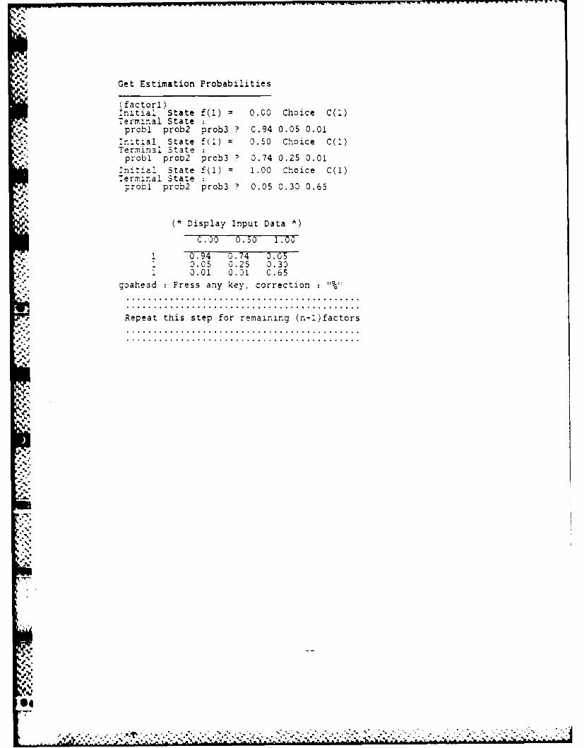
c. Estimate the probabilities using expert judgement
Using expert judgement, estimate the probabilities -pi , PJ c(k), where j1,2, 18 and "j Bpi , pi c(k) = 1. Repeat for elements S and E. This gives ipi , pj
c(k) ,and pi, pj c(k). Given Pi = 0 and C(I), Pi may transit to a new state P
where Pi can be 0, 0.5 or 1.0. Bv examining historical data and gathering advice from
senior officers or military experts, assess the degree of influence of changing attacking
forces on Pi and translate the assessment into matching probabilities, P0 ,0 C(I), PO
05 C(1), PO 1 C(I), with which each of these three transitions can take place. In our*. I Case, These.probabilities are shown below.
i -Pp, pjC(1)
Initial State Pi = 0 Choice C(l)
Terminal State
P =0 P =0.5 P= 1.0
0.98 0.01 0.01
The values shown in the table implies that if there are no major problems
regarding offensive operation at the present time (since Pi = 0), then the chances are
low that new problems might occur merely on account of changing attacking forces.
We now consider Si , the effectiveness of solutions. Let S, = 0 be the
initial state of Si. Focus on the same choice C(l). As before, we estimate the values of
so 0 C(l), SO 0'5 C(l), so , 1'0 C(l). Their values in our case are shown below
L5p * ,C(l)P1 Pi
_". Initial State S, = 0 Choice C(1)
Terminal State, S =0 S= 0.5 S 1.0
07-01.. 0.97 0.02 0.01
..
-
. . . . . . .
We also consider Ei , the potential energy of participants that has only 2
scale points. Let Ei = 0 be the initial state of Ei. consider on the same choice C(I).
Their values in our case are shown below
I pi ' pC(l)
Initial State Si = 0 Choice C(l)
Terminal State
Ej =0 Ej = 1.0
0.95 0.05
I 2. Transition Probability Matrix
Use formula 2.1 to compute the row of the transition probability matrix, ql-
C(l), corresponding to state Z, and choice C(l). In this step, we consider all the three
elements discussed above together to generate the joint transition probabilities, for the
initial state Z 1 (0,0,0) of the battle field, due to changing attacking forces. Repeat to
generate an transition matrix for the remaining 17 states. Table 4 shows the transition
probability matrix of Z 1. The upper part of this table is an application of formula 2.1
in connection with changing attack forces and the lower part is for the remaining
-r choices. C(2). C(3), and C(4). The remaining transition probability matrix. Z,.. ZIS
will be shown in Appendix C.
3. Goodness Measure
The goodness measure for each state is computed using formula (2.2). The
resulting g values for our example are given in Table 5. As shown in Table 5, state Z6
represents the ideal state in that it yields the highest possible benefit, i.e., g= 2.
I Conversely, the anti-ideal state, ZI 3 is the most adverse state for the organization
since the corresponding benefit is the lowest.
4. Transition Benefit MatrLx
I. Based on the transition probability matrix and the vector of goodness
measure, compute the transition benefits using formulas 2.3 and 2.4.. The result of
performing this procedure for all the initial states is shown in Table 6.
, 29
TABLE 4
TRANSITION PROBABILITIES INZ
Computation of Transition Probabilities qlj C(l)
Initial State: Z1 =(Q,Q,Q); Choice C( 1):Changing forces
Terminal State Formula Transiti-on prob.
0.,000. ., Q* ,O* 0. 0980970.50.0370.0,0.0,1.0 .0,.0*.0,.0*.0,. 0.98*0.97*0.05=0.07303.0,0.5,0.0 .0,. Q*.01.5*. 01.0 0.98*0.02*0.95=0.018620'0.0,0.5,1.0 .0,.0*.0,.5*.0,1. 0.98*0.02*0.05=0.000980f0.0,1.0,0.0 .0,.0*.0,1.*.0,.0 0.98*0.01*0.95=0.0093100.0,1.0,1.0 .0,.0*.0,1.*.0,1. 0.98*0.01*0.05=0.0004900.5,0.0,0.0 .0,.5*.0,.0*.0,.0 0.01*0.97*0.95=0.0092150.5,0.0,1.0 .0,.5*.0,.0*.0,1. 0.01*0.97*0.05=0.0004850.5,0.5,0.0 .0,. 5*. 0,. 5*. 0,.0 0.01*0.02*0.95=0.0001900.5,0.5,1.0 .0,.5*.0,.5*.0,1. 0.01*0.02*0.05=0.0000100.5,1.0,0.0 .0,.5*.0,1.*.0,.0 0.01*0.01*0.95=0.0000950.5,1.0,1.0 . 0,. 5*. 0, 1. *.0,1. 0.01*0.01*0.05=0.0000051.0,0.0,0.0 .0,1.*.0,.0*.0,.0 0.01*0.97*0.95=0.0092151.0,0.0,1.0 .0,1.*.0,.0*.0,1. 0.01*0.97*0.05=0.0004851.0,0.5,0.0 .0,1.*.0,.5*.0,.0 0.01*0.02*0.95=0.000190'1.0,0.5,1.0 .0,1.*.0,.5*.0,1. 0.01*0.02*0.05=0.0000101.0,1.0,0.0 .0,1.*.0,1.*.0,.0 0.01*0.01*0.95=0.0000951.0,1.0,1.0 .0,1.*.0,1.*.0,1. 0.01*0.01*0.05=0.000005
Transition Probabilities qlj c(k)
State Z, qlj C(k) for j = 1, ... ,18; k =1, ... ,4
state C(1) C(2) C(3) C(4)
1 0.903070 0.039200 0.617400 0.0180002 0. 047530 0. 156800 0. 264600 0. 0720003 0.018620 0.137200 0.061740 0.0360004 0. 000980 0. 548800 0. 026460 0. 1440005 0.009310 0.019600 0.006860 0.0060006 0. 000490 0. 078400 0. 002940 0. 0240007 0.009215 0.000400 0.006300 0.0360008 0. 000485 0. 001600 0. 002700 0. 1440009 0. 000190 0. 001400 0. 000630 0.072000 1
10 0.000010 0.005600 0.000270 0.28800011 0.000095 0.000200 0.000070 0.01200012 0.000005 0.000800 0.000030 0.04800013 0. 009215 0. 000400 0.00630C 0.00600014 0.000485 0.001600 0.002700 0.02400015 0. 000190 0. 001400 0. 000630 0. 01200016 0. 000010 0. 005600 0. 000270 0.04800017 0.000095 0.000200 0.000070 0.00200018 0.000005 0.000800 0.000030 0.00800
.%J%
TABLE 5
EVALUATING GOODNESS MEASURES
State (Zi) (Pi Si I Ei) gi
1 0.0 0.0 0.0 0.02 0.0 0.0 1.0 1.03 0.0 0.5 0.0 0.54 0.0 0.5 1.0 1.55 0.0 1.0 0.0 1.06 0.0 1.0 1.0 2.0 ideal7 0.5 0.0 0.0 -0.58 0.5 0.0 1.0 0.59 0.5 0.5 0.0 0.0
10 0.5 0.5 1.0 1.011 0.5 1.0 0.0 0.512 0.5 1.0 1.0 1.513 1.0 0.0 0.0 -1.0 anti-ideal14 1.0 0.0 1.0 0.015 1.0 0.5 0.0 -0.516 1.0 0.5 1.0 0.517 1.0 1.0 0.0 0.018 1.0 1.0 1.0 1.0
TABLE 6
TRA-NSITION BENEFIT MATRIX OF ALL CHOICES
State Z Choices C(k)
State C(1) C(2) C(3) C(4)
1 0.055000 1.235000 0.340000 0.8000002 -0.005000 0.425000 -0.010000 -0.3000003 0.175000 1.180000 0.580000 0.4000004 0.115000 0.370000 0.230000 -0.7000005 0.020000 0.770000 0.270000 -0. 1000006 -0.040000 -0.040000 -0.080000 -1.2000007 0.160000 1.595000 0.750000 1.2000008 0. 100000 0.785000 0.400000 0. 1000009 0.280000 1.540000 0.990000 0.8000C0
10 0.220000 0.730000 0.640000 -0.30000011 0.125000 1.130000 0.680000 0.30000012 0.065000 0.320000 0.330000 -0.80000013 0.090000 1.600000 1.045000 1.70000014 0. 030000 0. 790000 0. 695000 0. 60000015 0.210000 1.545000 1.285000 1.30000016 C.150000 0.735000 0.935000 0.20000017 0.055000 1.135000 0.975000 0.80000018 -0.005000 0.325000 0.625000 -0.300000
31
5. Generate the long run choice policy
The objective of this step is to determine the offensive operation policy by
evaluating what choices result in highest benefits in the long run as the battle field
stochastically transits from one state to another. The mathematics of maximization of
the long run benefit, when the law of transition shown in Table 4 and benefit function
,hown in Table 6 are known, can be achieved using Howard's algorithm. Let's trace
the !ong run choice policy by applying formula 2.4.
a. Initialize policy table
'U. Select best choices for each state from the benefit matrix that has
maximum value among C(1) thru C(5), and set up a policy table as the following table.
Origin Choice Policy Table
S1 S2 S3 . . S, S8 S9 SI ... S15 S16 S17 S18
S2 2.. 2 2 2 2 ... 2 3 2 3
b. Resolve variables and evaluate max property
Once we have resolved all the variable values (v(I), ... v(IS), g) using
gaussian elimination method (Ref, 81 we check to see if these resolved values satisfy the
maximal property expressed in formula 2.4. For each state-action pair S,a, we evaluateiiS.a) - g , v(s)qs , s C(a) and then for each state S choose the maximizing act "a'"
rRef. 1. This leads to
State i(S,a) V v(s)q S , s C(a)
( 1.1) 0.055-g+0.903070v(l)+0.047530v(2).. =I.OOE+00 - g
( 1.2 1.235-g+0.039200v(l)+0.156800v(2).. =l.OOE+00 - g
1,3) 0.340-g+ 0.617400v(l) + 0.264600v(2) ..= .0QE--0 - g. (1.-) 0.800-g+ O . SOOOv( )+ 0.072000v (2 . = .00E + 00 - g
' ), 1 2 20- g - 0.0090 19 v(2) - 0. 0o1 S I v(3 = -6.25 E- 16 - g
I !),2) ().- 0 g - 0.O(IO( "h v 21 - 0.0069 O v(3) 1... . .. 50E- 15 - g
.
(10,3) 0.640-g + 0.000400v(2) + 0.007600v(3).. =-1.62E- 15 -g
(10,4) -0.300-g + 0.006000v(2) + 0.01400O(3),. = -8.60E- 16 - g
... ... .,. ....
c. Set a new policy table
At the above step, we observed a new policy, marked by the asterisks and
they are
New Choice Policy Table
SI S2 S3 ... S7 SS S9 SIO ... S15 S16 S17 S18
2 4 2 .. 22 1 ... 2 3 1
,. *J.
d. Compare a new policy table with a previous one
Repeat b) and c) until a new policy table and a previous policy table
correspond each other or the maximal income per unit time (g) is decreased. The latter
case ,occasionally happens, and is possible in the case of g value near zero. For this
unstable state, we set recursively arbitary Vi.1 equal to 0, and repeat a) thru c).
e. Test result
As a result of prescriptive garbage can model execution, we lay down a
policy table shown in Table 7 that have solved expressed by formula 2.5. Givcn Table
7 recommend and advise the commander of the best choices available in a specific
organizational state. For example, if given situations are (i) Acute shortage of
attacking forces, big mission load, a tremendous time delay to the consequent
operation, (ii) Most of personnel have no experience in the battle field, poor
coordination with adjacent, poor performance weapon systems, (iii) Not quite proud oftheir operations, we would like to change attack forces known as choice 4 to achieve
his goal. Like this we can select choice I (do smoke operation) in state 6,10,18, choice
13
.. '--I' ./f.',,- $7 ** * %* ,./< .- ** . . . * . . . ,.. . .- •.-,- . , -" ," .,.,r -" '.-'.-' ,' -,.-,.'. . " " ." ",".".. v ..' ., '." -.." .' .'..,." ..." .''.'.',-; .- .-.".' " "'.."V*., .'"" .-
2 (supporting high performance weapon systems) in state 1,3,4,7,8,9.11,14,15,17, choice
3 (reinforcing attack forces) in state 12,16, and choice 4(changing attack forces) in state
2,5,13.
TABLE 7
SELECTED CHOICE POLICIES
State Choice Policyzi C(k)1 22 43 24 25 46 17 28 29 2
10 111 212 313 414 2
-" 15 216 317 218 1
'3-.
4
IV. FURTHER RECOMMENDED STUDIES
This thesis considers a prescriptive garbage can model to advise the participantsof the choices available to them in a specific organizational state, and implements it togenerate a choice policy table. The current system covers chance events resulting fromthe interactions of four elements in the organizational context, (i) problems, (ii)
,," solutions. (iii) participants, and (IN-) choice opportunities. The computer program couldbe modified to process a greater number of organizational states depend on a memory
allocation(current system maxchoice 5, maxstate 36).An ideal PGCM wouid be one that interfaces with an expert system to
automatically transfer estimation probabilities and feasible actions about the
.organ izationproblem into PGCM system without human intervention. The following.* diigrarr shows how an expert system would be used.
DecisoMae
estimation prob
alternati.ve actions
Expert Sy~stem P. 3. c. Mswppy estirnation-
processprob. and actions
Results
- Interface between Expert System and PGCM
A, exper: s',s'em uses methods of reasoning to eliminate bad courses of acticns.-nJ :0 detor-, e :e best courses of actions to achieve a goal. Expert systems use
,. in an inae.l:.ent way, to perform tasks that are normally associated with
i *... v.
• a~o • .i. -,. .
0 . , , . . . , . - . . . . , , - ., .,4€ ., , . . - - . - ., -. ' - .-% .. " ' " ' r ' ' . . .- . .. ......
human experts. There are many anarchic and random situations, but human experts
have some difficulties to find the best choice every time. Hereby we illustrated a
diagram as one possible model to interface between PGCM system and expert system
to determine the best actions for the given set of organizational states. The next step
in this study is how to interface an expert system to estimate transition probabilities
and feasible actions for input to the prescriptive garbage can model.
.%
..
APPENDIX A
A SOURCE PROGRAM
PROGRAM PGCMPROG(Input, Output);$(*s 400000 *)
** TITLE : PRESCRIPTIVE GARBAGE CAN MODEL **** AUTHOR : Maj Kang, Sun Mo **** Date Written 11 Feb - 19 May 87 **
** Product : Version 1. **** System Used : IBM 3033 VM/CMS **
** I/O Process : Terminal Keyboard **
** Description : This program is an interactive **** choice processing system to support **** decision makinq by using Prescrlptive**
Garbane Can Model **
V. (** Global Constants **)const
zero O;one 1;two 2,three 3;four = 4;six = 6;eight = 8;ten = 10;seventy = 70;maxfactor number of variablemaxchoice 5 number of maximum choice for each statemaxscales 5 number of maximum scale point for one factormaxstate = 36; number of maximum statesmaxstateetc 37; * number of maximum states plus onemaxrow = 180 * number of maxsrows, max-s ate*choice
typecounter = 0..maxint;inputtype = recordline array(.one..seventy.) of char;length counter;las counter;
end;commands = (EXECGCM, EXECEXIT, BAD);usermsgs (BADLINE, NOINPUT, NOINTERACT, ETCVAL, ETCCHO,
NONNUM, OVERSTATE, IMPOSSIBLE);choicetable = array (.one..maxstate.) of integer;transitiontable=array( .one..maxrow, one..maxstate. of real;benefittable = array .one..maxstate, one..maxchoice.) of real;policytable = array(.one..maxstate.) of integer;
(** Global Variables **)var
possiblestates,int, vi integer;gain real;wait char;choices choicetable;tranmatrix: transitiontable;benematrix: benefittable;
37
* •
~### G C M PART 1.## Functions ##
* Function Getinp*-------------------------------------------------------
Function getinp(var userinp : inputtype):boolean;(* Get a single-letter command,
making sure it is in the set of valid commands *)vatbegich char;
beginuserinp.length 0;userinplast 0;if eof then getinp := false
else beginwhile not eoln do begin
read(ch);if userinp.length < seventy then begin
userinp.length := userinp.length + 1;
end userinp.ine(.userinp.length. ) ch;
end;readln;
end;getinp := true;end; (*getinp *)
==Function Skipblanks **---------------------------------------------
Function skipblanks(var userinp : inputtype):boolean;a blank : boolean;
begin1eqbank := true;
while (userinp.last < userinp.length) and blank do beginuserinp.last := userinp.last + 1;i '- if userinp.line(.userinp.last.) <> ''then
blank := falseend;if not blank then
userinp.last := userinp.last - 1;skipblanks := blank;end; (* skipblanks *
= Procedure Getchar *
procedure getchar(var userinp:inputtype; var ch:char);eginIf userinp.last < userinp.length then begin
userinp.last := userinp.last + 1;ch := userinp.line(.userinp.last.);
end elsech
end; (* get char *).4
* Procedure Writeuser
Srocedure writeuser(msg:usermsgs);podegn
case msg of
39
.4
BADLINE : writein 'Bad Input, try again <press enter key>'NOINPUT :writein 'Have no data, try again <press enter key)'1NOINTERACT: writein 'Nothing typed, tr again, <Press enter key>'NONNUM writei 'Nonnumeric data, ry again <press enter key>'ETCVAL begin
w rite ('Available scale point :2 to 9, try again')writein ( '<Press enter key>');
end;ETCCHO begin
write ('Available choice :2 to 5, try again ');write.n ('<press enter key>');
end;
OVESTAE bginwrite ('Maximum organizational states is less')writein ('than 36, try again <press enter key>')
end;IMPOSSIBLE: begin
write ('Cannot set up, try again with new data ')writeln ('<press enter key> )
end; end;reand wi
end;
Function Getcommand
Function getcommand(var command:commands) :boolean;* (* Get a single-letter command
make sure it is in the sei of valid commands *var
ch char;
* beginp: inputtype;
page;
t"rite2.n '* * :67writen '~GCM Program options are the followingswrtin~ ------------------------------------------------------
w4rite~ln '*
wrte).n '** 1. ExecGCM (Execute GCM Program :67writn ) *':67)
writein ' ~2. ExecExit(Execution stop ***:67wr~te2.n ****:6wr ieln ===== Type ,Number !!!!***' :67writeln l* :******************** 6cetcommand :~false;cormmand := BAD;if qetinp(userinp) then begin
*getcommand := true;if not skipblanks(userinp) then begin
getchar(userinp,ch);if skipblanks(userinp) then
if ch in (.1,12.) thencase ch of
Il'l command :EXECGCM'2' command EXECEXIT;
enden;else getcommand :false;
nd;end;
40
~. -. "
F.'- , ## ##-.. ########################################*
- * ### G C M PART Ii. ###*## Generate Matrix ###*### ###
•### generate transition probability, ## ** ### transition benefit probability, ### *4## organizational states, goodness ### *
• ### measure table: Input for Part III ### *• ################## #####t## ###
(***** GET TRANSITION, BENEFIT MATRIX ***
, '., Procedure Getmatrix(var possiblestates:integer; vat choices:choicetable;J var tranmatrx:transitiontable; var benematrix:benefittable);
, constmaxi-row = 45;
tye scaletable = array .one..maxfactor.) of integer.
scalevaltable = array one. .maxscales, one..maxscaies.) of real;estimationtable=array(.one..maxfactorone..maxirowone..maxscales.)
of real;combination = record
column : array (.one..maxfactor.) of real;end;
statematrix = array (.one..maxstate.) of combination;goodnessmatrix = array (one..maxstate of real;
varnumfactor,maxcho : integer;scales scaletable;scalevals scalevaltable;statmatrix : statematrix;goodmatrix : goodnessmatrix;estmatrix estimationtable;
*i ****************************************** *}
-.'.* Get Number of Factors * *v. . ***************************************** *
Procedure getnumoffactor(var numfactor:integer;var possiblestates:integer;var scales:scaletable);
vari : integer;ch char;indomain : boolean;
,.[ === Function Get Max # of States =
Function Getmaxnum(num : integer; scales : scaletable):integer;varb base, i : integer;:'" begin
base : one;for i : 1 to num dobase : base * scales(.i.);
getmaxnum := base;end;begin teln Number of factors : 3 -- P, S, E';
writeln ' __;writeln;
e'.i numfactor := 3;writeln 'Enter # of scale points for each factorwriteln___
v '- 41
.-4,
writein;(********get number of scale point*******)
indomain:=ale* I epeat (*repeatI
repeat (*repeat 2*)goodvalue :=false;writeln(Ifactor',i:2,'if getinp(userinp) then
beginJ, if not skipblanks(userinp) then
begingetchar(userinp,ch ;if skipblanks(userinp) then
if ch in (.''', ,5,6'''''')thenbegin
case ch of'2': it :2;'3' : mt :3;'4' int 4;'5' : mt 5,'6' : mt :6;'7' : mt :7;'8' : mt :8;-'9' : mt :9;
end; (*caseend*)g oodvalue := true;
enc (*endif ch*)else writeuser(ETCVAL) (*else ch*)
else writeuser(ETCVAL) (else shipblanks*)6 end (*endif notskipblanks *)
* else writeuser(NOI NPUT) (*else notskipblanks*)end (*endif qetin *
else writeuser (9QINTERACT); (*else getinp*)- if goodvalue then
beginscales(.i.) := int;
end. i+;
until (i =numfactor+one); (*end repeat2 *(********check and correct scale point*****)
repeat (*repeat3*)writeln('# of scale points arezor i := one to numfactor do
writeln(Ifactorl,i:2,1 : 1,scales(.i.));writeln('goahead : Press any key, correction:writeln; writeln;readln(ch ;if ch = '-.' then begin
writeln('Enter factor number and valuereadln(l, scales (.i.)); end;
until not(ch =I);(*end repeat3*)possiblestates := qetrnaxnum(numfactor, scales);indomain := (possiblestates <= 36);if not indomain then writeuser(OVERSTATE);
until indomain; (*end repeat 1*)end;
"~ '"'~ Get Number of Choices
Procedure getnumofchoices(numfactor:integer; possiblestates:integer;var choices:choicetable; var maxcho:integer);
vari :integer;ch : char;
begin
42
A .A'I -
write 'Get Number of Choices for each State Z(i) ')
writelnIi = 1 ..',possiblestates:3); )
N ~~~~write I____________________________writelrxi' ______ ); writeln;
(********get number of choice *******)I1: 1;repeat
Ngoodvalue :=false; I* writeln('Statel,i:3,* if getinp(userinp) then
beginif not skipblanks(userinp) then
begingetchar(userinp~ch ;if skipblanks(userinp), then
Aif ch in (.121,13', 4,5.) thenbegin
case ch of'2' mnt 2;'3' mnt 3;'4': mt :4;'5' : mt 5;
end; (*caseend*)g oodvalue := true;
end (*endif ch*)else wz-iteuser(ETCCHO) (*else ch*)
else writeuser(ETCCHO) (*else shipblanks*)end (*endif notskipblanks*)else writeuser,(NOINFUT) (*else notskipblanks*)
end (*endif getinp*else writeuser (NINTERACT); (*else getinp*)iJf goodvalue then
begichoices(.i.) :=int;
i + 1V end
until (i = possiblestates+one); (*end repeat2 *(********check and correct
writeln('State ZWi # of choices')writeln(
V repeatfor i :=one to possiblestates do
writeln(i:6, choices(.i.):20);writeln('goahead :Press any key, correctionwritein; writein;readln(ch .,if ch = '-. then begin
writeln( 'Ernter state number and valueUnreadln(i, choices(.i.)); end;utlnot(ch =V;
maxcho :-999;for i one to possiblestates do
if choices(.i.) >maxcho then maxcho choices(_'.);end;
GtEstimate Probability
Procedure getestprob(numfactor:inteqer; maxcho:integer;scales:scaietable; var scalevals:scalevaltable-
var var estmatrix:estimationtable);
i,j,k,l,m,n :integer;
S~p real;ch char;
* ~ Get scale points of each factor
'4
'Ip.q2~ *- ~"d ~ ~ ** ** ~ *.:**<~~
Proedue Gtvrounda(p u~ntg *a 100);ssclvatbl)
begin :rel
for i one to m dofor j on to numfactor. dobei
for vas(1,. one to/100s; j d
be ingevaofc wriumate ' r ob',J.:1, ); wienGet ra estimation probaility*****
for 1 := one to scale(.j. do
beginn
write(' ':10);for k := one to sales()j') do
write I'------al wrteln
* writel (scalevals(.j k)T6:, I ~); wit;write "eria ':0)for k := one to scales(.j. do
write (------');wr Iln. lnforea koetiatison. proilt
or 1 := one to scales(..) do'MW red(estmatrix(.j,(i-l)*scales(.j.)+lkl.):6:,
rieln;end; (*end k*) writen; wien
crt~nhcand coPressaykytcreto
write I ---- 1)iei ; wie
f ch := 'on' th cen (j begiw ritnte Chicro,0o,)ro;fo stka:=ione to lkscales(.j.) lm. do; nd
* ~ ~ ~ ~ ~ rt (I------------------------------ ------*eln
w= rcd r G ~e StaeMatrix *,iilcls(j)kl)62
write4.4
en;'en * wien
procedure Getstatmatrix(numfactor:integer; possiblestates:integer.scajles:scaletable; scaJlevals:scalevaltable;
var statmatrix:statematrix);var
i ,Kb- ptr, loop, mult : integer;
for oneto numfactor do
Tut mult *scales(.i.);loop possblesatesdiv mult;
f:-or := one to rnult do? begin
ptr :=ptr + ofle;if p tr > sca2.es(.i.) then ptr :(ptr mod scales(.i.));for k := one to loop do
end;am t i (.j l * o p k )co u n . . :s al v l (ip r )
end;end;
V.'Procedure Print State Matrix --
procedure printstatmatr.x(numfactor:ainteger; possiblestates:integer;statmatri.x:statematrix);
varcolp tr,
bgnsca leptr, tableptr integer;
page,-y wri.teln(' ____________ 7)
writein ( Organizationa Sae'57;writeln(___________'writein; writeln;writeln' ________________________ '.70);
-. writeln(' Number of factors : :49, numfactor 1)T;writein I State Combinations of Scale Values' :67).writeli (1_______________________ :70);for tableptr := one to possiblestates do
beginw4rite(' ':23); write(tableptr:6); write(' ':9);for Colptr := one to numfactor do
write( statmatrix(.tableptr.).column(.colptr.) :6:2, ' ':2);write in;
end;en writeln(I 1:70);
== Procedure State Matrixc for Help *=------------------------------------------ *
procedure printhelpfile(nurnfactor:integer; possiblestates:integer;var r, tblestatmatrix:statematrix);
begins ca~ epr Pt lptr : integer;
page;rewrite(helpfile, 'helpfile data,);writeln (helpfile, 'Organizational States' :38);write-In helpfile 1___________ :38);writein (helpfile5 ; writeln(helipfi e) ;write (helpfile,
.0
44
~v. writein helpfile,for tabieptr := one to possiblestates do
begin tbet6wiehelp file, -)
for Coip tr :=one to nLmfactor dowrite (helpfile,statmatrix(.tableptr.).column(.colptr.):6:2);
writeln(helpfile, ':2);end;
write (helpfile, _____________________I;
end;w riteln~ helpfile, I_____ )
9 * Procedure Transition Matrix *procedure gettrarimatrix(numfactor:integer; possiblestates:integer;
choices: choice table; scales: scaletable;* scalevals :scalevaltable-
estmatrix:estimationtabie;statmatrix :statematrix*
var tranxnatrix:transitiontable);var
mnit, next.cho, columns,pointer, firstptr, secondptr :integer;getprob, multiprob : real;found : boolean;
begin* for init := one to possiblestates do (*2oop0 *9.Ifor cho := one to choices (.init.) do ( * lop *)
for next := one to possiblestates do (* Lop3 *begin
mul tiprob:= 1;for columns i=one to numfactor do (*loop4 *begin
pointer :0;
firstptr 0; secondptr :=0;found :=false;while not found dobegin
pointer := pointer + 1;.if scalevals(.columns, pointer.)statmatrix (.init.) .column (.columns.) then
if firstLtr := pointer-ifscalevals(.columns 'pointeri)=
statmatrix(.next.).column(.columns.) thenfoundpr : pointer;found not (frtt~eodt)O
V end-secondptr := cho-l)*scales(.columns.)+ secondptr;getprob estratrix(.columns,secondptrjfirstptr.);mul tiprob :=multiprob * getprob;
end;end 'of loop4 *
tranmatrix(.(init-l)*choices(.init.)+cho,next.) :multiprob;end -(end of loop3 *
(end of loop2 *
end; (*end of loopi *
==PROCEDURE PRINT Transition Matrix =
.46
procedure printtranmatrix(pcssiblestates:integer; choices:choicetable;
tranmatrix:transitiontable);
ca olumns,init, next :integer;
beiparr: array (.1- 5.) of real;bgnfor init :=one to possiblestates do (*loopi *
beginpage-writeln ( _____:___ 47)write n (:Transition Matrix'A:4);writein' 1 __________ :47)write ln;write in;writein ('Initial State :Z' ,init:3);wrjt ' ' t_ _ _ _ _ _ _ _ _ _ _ _ _ _ _ _ _ _ _ _ _ _ _ _ _
writeln( ___________ )
wrte ' statefor columns := one to choices(.init.) do
write('C(' ,columns:1,')', .1 :13);write in;write ('________________________________writeln('____________ )
* erase *or columns :=one to choices(.init.) dotemparray(.columns.) := 0;
for next :=one to possiblestates do (* loop2 *beginwrite (next :4);for columns := one to choices(.init.) do beqin (*loop3 *
write(tranmatrix(.(init..1)*choices(.init.)+columns, next.):14:
(*erase *temparray(.columns. temparray(.columns. +
tranmatrix(I(init-l)*choices(.init.)+columns, next.);end; *edof o3
writeln;end.(end of loop2 *
writel ----------- -------- - - - - - -- )
end;end end of loopi *
- = Procedure Do Goodness Measure --
procedure Goodnessmeasure(numfactor:integer; possib3.estates:integer;statmatrix :statematrix;
var goodrnatrix:goodnessmatrix);var
index,ideal, anti : integer;temp,max, min : real;
Procedure Print Goodness Matrix =
procedure printgoodmatrix;ccnstne=1
427
-p.
*31L_
two =2;four= 4;eight=8;var loop,
row, col : integer;begin
page;writeln _ __writein Goodness Measurements*d ritelnL __ _ __ _ __ _ __ _ _
writeln;writeln.Swrite ( _________________ );
w:riteln( );
* write (' State Combination ');writeln(' ':(numfactor-two)*eight+four, 'Goodness Remarks');write (' Z(i) 1);for loop one to numfactor do
write('val',loop:1,' ':4); writeln(lvalue');write (' );writeln (' );for row := one to possiblestates do
beginwrite(row:6);? write(i 1:9 ;for Col := one to numfactor do
write( statmatrix(.row.).column(.col.) : 6:2, ' ':2);writekgoodmatrix(.row.) : 6:2, ' ':2);if row = ideal then write(' ':5, 'ideal')
else if row = anti then write(' ':5, 'anti-ideal');writeln;
end;writeln()" I end;
(** Procedure Begin **)begin
max := -999; min : 999;for index := one to possiblestates doe beginb Case numfactor of
2 : writeln('* Not prepared *');3 : begin
temp := -(statmatrix(.index.).column(.one.))+(statmatrix(.index.) .column(.two.))
+(statmatrix(.index.).column(.three.));goodmatrix(.index.) := temp;if temp > max then
beginmax := temp; ideal : index;
end;if temp < min then
beginmin := temp; anti : index;
end;end;
4 : writeln('* Not prepared *1);end. (* end case
end; (* end for *)end; Printgoodnatrix;
* == Procedure Get Benfit Matrix =
procedure getbenematrix(possiblestates:integer;
48
S4
.
choices :choicetable;tranmatrix: transitiontable;goodm'atrixigoodnessmatrix;
var benematrix:benefittable);var
row, col, loop :integer;tep real;
bei or row :=one to possiblestates do (*loopi *for col :=one to choices(.row.) do (*loop2 *
begintemp := 0;for loop :one to possiblestates do (~loop3 *
temp :=temp+(trannmatrix(.,(row-l)*choices(.row.)4col,loop.)*(goodmatrix(.loop.) - goodmatrix(.row.)));
benematrix(.row col. /- epend of loop3 tmp
(*end-o oo2*(en of loop *
end; edo op
==Procedure Print Benefit Matrix =
procedure printbenematrix(possiblestates:integer; maxcho:integer;choices~choicetable; benematrix:benefittable);
varbgnrow, col : integer;
page; '4writen(' 1:4writeln;'IBSeneft Matrix'1 :47write -in( ' ___ ____':47)
writeln;wr ite In;write ('State ZWifor col := one to maxcho do
write('C( ',col:1, ') ',' ':10);wr ite in;write ____________)_____________________
r ~~~~rltein _____________
for row := one to possiblestates do ( loopi *begin
write(row:4);for col := one to choices(.row.) do (*loop2 *
write(benematrix(.row,col.):14:6);(end of loop2 *
writeln;e4of loopi *
writein~
end,
(*** PART II. MAIN PROGRAM **
begin.========----In ut Data via Terminal---Step I. *
Getnumoffactor (numfactor ,possiblestates scales);Getnumofchoices (numfactor~possiblestates~choices maxcho);Getestprob (numfactor,maxcho~scales,scalevals,estmatrix);
Get Transition Matrix- ----
Getsta natrix(numfactor,possiblestates,scales,scalevals,statmatrix);printstatmatrix(nujmfactor ,possiblestates ,statmatrix);
* .49
% %x>.
- - -, - - -- - C
pi-inthelpfile (numfactor,possiblestates,statmatrix);(* Step III. *)
* ~Gettraninatrix(nurnfactor ,possiblestates ,choices, scales, scalevals,* estmatrix,statmatrix,train'atrix)
Printtranmatrix(possiblestates ,chioices, trar.ratrixY;
-------------------Get Benefit Matrix-----(Step IV. *)
Goodx.essreasure(nuifactor,possiblestates,statrnatri-x,goodmatrix);
(*Step V. *Getbenematrix (possiblestates,choices,trannatri.x,
goodmatr.ix, benematrix);* printbenernatrix(possJ.ibjlestates,maxcho,choces,benenatrix);
end,:
50)
* # # * # # * # # # # # # # # # # ####### ##### G C M PART III. ###
### Generate Long Run Policy ###### This part processes howards algorithm ###### main modules are Dynamic formulation, ###### Resolve variable, and Setnewaction ###
( * * GET CHOICE POLICY * *
Procedure Getchcice(possiblestates:integer choices:choicetable;tranrnatrix:transitiontable;benematrix:benefittable; var policy:policytable);
type markovtable = array (.one..maxstate, one..maxstateetc.) of real;determinval = array (.one..maxstateetc.) of real;
varindex integer;1,j ; integer;maxincome real;markov markovtable;resolution determinval;newpolicy policytable;reached, matched,quitnow, inforced boolean;
(*== PROCEDURE Initialize policy Table == *
*---------------------------------------------
procedure initialize(possiblestates:inteqer; choices:choicetable;benematrix:benefittable; var policy:policytable);
varrow, col : integer;max : real;for row one to possiblestates do
beginmax -999;for col := one to choices(.row.) doIf benematrix(.row,col.) > max then
beginmax := benematrix(.row,col.);policy(.row.) := col;
end;end;
end; I* *IPROCEDURE Dynamic Formulation ==( == = == = = = = ============: -- - - - -- - - - - *) e t t s i t q r
procedure dynamicformulation(vi:integer; possiblestates:integer;choices:choicetable; tranmatrix:transitiontable;benematrix:benefittable; policy:policytable;
var markov:markovtable);varbeginrow, col : integer;
(* fil matrix with variable coefficient *tor row := one to possiblestates do
markov(.rowone.) := 1.0;for row := one to possiblestates do
for col := one to possiblestates doif row col then
narkov(.row,col+1.)i-(tranmatrix(.(row-l)*choices(.row.)+policy(.row.),col.))
else
51
markov(.row, col+l.)-(tranimatrix(. (row-i )*choices(.row.)+policy(.row.),col.));
for row :=one to possiblestates domarkov(.row,possiblestates+2.) :=benematrix(.row,policy(.row.).);
Sremove an arbitary vatiable v(i) *or row :=one to possiblestates do
for col :=vi + one to possiblestates + one doend; markov(.rowcol.) :=markov(.row,col+l.);
* PROCEDURE Resolve all variables =
procedure Resolvevariable(vi:integer; n:integer;var mar ov:markovtable;var resolution:determinval);
varj , integer;
mu tfac,
begin~ el(~******manipulate markov matrix ******
for i 1= to n-i do beginif rnarkov(.i,i.) <> I then
beginmnu' Itfac :=l/(markov(.i,i.));for i : i to n+1 doen;markov(.i,j.) := markov(.i,j.) *multfac;
for j.: i+1 to n dobegin
muitfac :=markov(.j,i.);fcr k :=i to n+1 doen;markov(.j,k.) :=markov(.j,k.) - (multfac *markov(.i,k.));
end;
(*******find solution******)resolution(.n.) :=markov(.n,n+l.)/markov(.n~n.);for i : n-i ownto 1 do
begintemp 0for i +1 to n do
tep = em +(markov(.~. resolution(.j.));resoution(.i.) :=markov( .i)-tep
end;1.-tep
for jn downto vi + 1 doresolution(.j+l.) :=resolution(.j.);
resolhuton(.vi+l.) :=0;end;
PROCEDURE Set New Action =
proced ;re setnewaction(possiblestates:integer choi0ces:choicetable;tranmatrix: transitiontable;benermatrix:benefittable;resolution:determinval; var newpolicy:policytable;policy:policytable);
type-val-propertv =recordptr integer;
%.- real.;
var
.152
'4W
~ :..K r:,Z
Mr U, -- -- W
col, cho loi..j'k,seiectode: integer-,temp,dynamic,max: real;
be property : array (.one. .maxchoice.) of eval..property;
for loop one to possiblestates dobegin
max -999;for cho :=one to choices(.loop.) do
begindvnamic 0;fbr col one to possiblestates do begin
dynamic:=dynamic +(tranmatrix(.(loop-l)*choices(.loop.)+cho~col.)*
resolution( .col~ione.));end;dynamic:=dynamic + benematrix(.loop,cho.)property (.cho.) .ptr :cho;
property( .cho.) .val :=dynamic;end ( * end of choice *Ssorting *)or i :choices(.loop.) downto two dofor j :one to i-i doif property(.i.).val > property(.j.).val then begin
temp :=property(.j.).val;property :1: val roperty(.i.).val;
* ropertyki.vl epK property(.j. .ptr;
property(.:.)ptr: property( .i.) .ptr;pr er: k;r end
* I if Yprope~ty(.l.).val >= 0) and (property(.2.).val >= 0) thenselectcode := 1;
if (property(.l.).val >= 0) and (property(.2.).val < 0) thenselectcode :=2.
*if (property(.l.).val < 0) thenselectcode := 3;
case selectcode of1. if ((property(.l.) val-property(.2.).val)/
property (.1.).va 1) <= 0.0001 then (* identity *newpolicy (.loop.) := policy (.loop.)
else newpolicy( loop.) := property(.1. ) ptr;2 ne'policy(.loop.) := roperty(.l.). Htr;(* nonidentity *3 : if ((property(.2. )val-roperty (.1.).val)/
property(.1.) val > 0.0001 then ( nonidentity *newpolicy (.oop,) :property.1)pt
en;else newpolicy~ .1oop.): policy(. loop.)
end; (* end of loop *end;
(**PART III MAIN PROGRAM" **
begi~nvi :=possiblestates;repeat
fnitia~ize (poshsblestates,choices,benematrix,policy);maxincome : -999.0;inforced :false;repeat
1* Step 11. *Dynamic formulation(vi,possiblestates,choices,
(* Seo ~)tranmatrix, benematrix, policy, markov);Reso.vevari-able(vipossiblestates ,markov, resolut ion);for 1 :-_ 1 to possible states + 1 do
(~Step 1'J. ~setne'act' on(possiblestates,choices,tranmatri x,benematrix,
..... . . -. .- .~ .. .
-. * .. ..t .* *..*-- . - - .--- .** . . . . . *%
resolution,newpolicy,policy);quitnow false;if maxincome <= resolution(.one.) then
begini1ndex :=0;quitnow true;repeat p
index index + 1;reached (index >= possiblestates);matched (olicy( .index)=newpolicy(.index.));q uitnow quitnow and matchedjpicy(.index.) :=newpolicy(.index.);
until reached;if cquitnow and (resolution(.one.) < 0) then inforced true
else maxincome :=resolution(.one.);4 end
utlelse inforced :=true. (*endif maxincome*)utl(guitnow or inforced)>
if (vi = O and (not quitnow) then writeuser(IMPOSSIBLE);until ((quitnow and (not inforced)) or (vi~o));
Vi=v I + I1gain resolution(.one.); (*printed on policytable*)
end;
4'4
. , ##########################################,',## # ###
"### G C M PART IV. ###, ##########################################
*****I N T E R A C T 1 0 N * ***
Procedure interaction(possiblestates:integer; policy:policytable);type elementtable =array one..maxfactor.) of real;
oneline = packed array(.one..seventy.) of char;var
current : integer;elements elementtable;line oneline;yesno char;
* doall, nomore,needhelp : boolean;
-------------------------------Do Partial Decision policy == *
------------------------------------------------------------ Iprocedure dopartial(possiblestates:integer; policy:policytable);begin
writeln('Do you want to see Helpfile for current problem ? y/n');readln(yesno);needhelp := (yesno='Y') or (yesno='y');if needhelp then begin
reset (helpfile, 'helpfile data,);while not eof(helpfile) do begin
readln(helpfile, line);enwriteln(line); end;end;
repeatwriteln('What is your current state ? ===> Type n');readln(current);
until (current > 0) and (current <= possiblestates);writeln;write ('Current State ', current:2, ', ');wr:teln('Best Choice ' , policy(.current.):2);writen;
end;
PRINT POLICY TABLE =
procedure printpolicy(possiblestates:integer; policy:policytable);var
begin loop, cnt : integer;
page;writeln_ ':27
%- writeln 'Decision Choices':27% writeln' _:27;
writeln;wri:eln;writeln 'State Choice Policywriteln 'Z(i) C(k) i;writeln;i' .. writeln.c t := 0;for loop := one to possiblestates do loop2
beginwriteln(loop:4, ' ':30, policy(.loop.):3);
55
.% % %
16A.
I - I F-. -- - -w -, - ---- - - -f~ r
cnt :=cnt + 1;if (cnt mod 3) = 0 then readln(wait);
end;I)wi-iteln(I _ _ _ _ _ _ _ _ _ _ _ _ _ _ _ _ _ _ _ _ _ _
wr-xteln;writeln('set arb2.tary v(', vi:2, ')to 0');writein;wrliteln('maxincome per period ',gain);
writein;
gage;
beainrepeat
page;wrniteln( 'Do you want all decision policy ? yin');readln(yesn )doall :=(yesno='Yl) or (yesno='y');ifdoall then printpolicy(possiblestates,policy)else dopartial(possiblestates,policy);
writeln( 'Do you have another ploblem ?)readln(yesno);nornore :=(yesno'Nl) or (yesno=ln');
until nomore;end;
56
### G C M PART V. #####Exit GraeCan Prod. ##
SGET BOOLEAN VALUE
Procedure Getboolean(var Exit:boolean);
x. t := true;page;
en;
End of Garbage Can Model ProQram ***)****************************
M MA IN P ROG R A M
beginQuitnow := false;While not quitnow do begin
if getcommand(command) then
Case command ofEXECGCM t begin
Getmatrix(possiblestates,choices,tranmatrixbenematrix);
Getchoice(possiblestates,choices,tranmattix,benematrix,policy);
Interaction(possiblestates,policy);end;
EXECEXIT : Getboolean(Quitnow);
endelse Writeuser(BADLINE);
end;end.
.57
fr-I
f.-.
- . .A m-- - - - - n
APPENDIX B
USER MANUAL
*" PGCM Program, 1987
I. PROGRAM NAME : pgcmprog (written in Waterloo pascal language)I. PURPOSE : Get a set of choices available in a specific organization
problemIII.TO USE:
1. Before Execution
1) Formulate problem and set alternative actions2 Turn on your terminal3 LOGIN userid4 ENTER PASSWORD(IT WILL NOT APPEAR WHEN TYPED):5 Memory extention (if necessary)
iDE STOR 1500kI CMS
6) Execute garbage can program: pw gcmprog pascal
2. During Execution
1) Select menu option1 ------ ExecGCM2 ------ ExitGCM
2) Enter number of scale points for each factori.e> factor 1 : 3
factor 2 2factor 3: 2
------> possible states :3 x 2 x 2 = 124) Enter number of choices for each state
i.e> state 1 ? 2state 2 ? 2state 3 ? 3state 4 ? 3state 5 ? 3state 6 ? 3state 7 ? 2state 8 ? 2state 9 ? 3state 10? 3state 11? 3state 12? 3
=====.> maxchoices : 34) Enter estimation probabilities
if user has the following input data,factorl(P) factor2(S) factor3(E)
P S Echo 0.0 0.5 1.0 cho 0.0 1.0 cho 0.0 1.0
F 0.2 0.4 0.3 1 0.106 0.30.61 0.3 0.5 0.5 1 0.9 0.4 1 0.7 0.41 0.5 0.1 0.2
chol 0.0 0.5 1.0 cho 0.0 1.0 cho 0.0 1.00L .1. 0.3 0.2 -T 0.5 0.1 2 -0,2 0.T
2 0.5 0.3 0.2 0.5 0.9 2 0.8 0.12 0.4 0.4 0.6
chol 0.0 0.5 1.0 cho 0.0 1.0 cho 0.0 1.0
-T 0.1 0.7 0.2 I0.8 0.3 --- .4 0.5
44.
3 1 0.1 0.2 0.3 3 I0.2 0.7 3 0.6 0.53 j0.8 0.1 0.5
Interact with the folowing manner
(factor1)Initial State f(1) = 0.00 Choice C(1)Terminal Stateprobl prob2 prob3 ?.2 .3 .5
rectangle : input dataInitial State f(1) = 0.50 Choice C(1)Terminal Stateprobl prob2 prob3 ?
S0.4 0.5 0.
Initial State f(1) = 0.10 Choice C(1)Terminal Stateprobl prob2 prob3 ?
0.3 .5 0.2
(factor2)
(factor3)
choice 2 and choice 3 operations are the same
.4, 3. After Execution
1) Do you want all decision policy ? y/nyes- display all choice policies
no
Do you want to see Helpfile for current problem ? y/nyes
,-isplay organizational states for memory aidsWhat is your current state ? === Type n
no
What is your current state ? => Type n
2) Do you have another ploblem ?yes
no to procedure 3.1no
go to procedure 2.1
4. Get results1) PRINT OUT
PRINT gcmprog listing
U-q'.'.'.59
.04
.... .,... ............ .. -....... -*-...- "4."2' "-"4** ' . .
APPENDIX C
OFFENSIVE OPERATION EXAMPLE
** Step I User Interaction **!-,. ** **
I. Formulate problem and prepare estimation probabilities
P Importance of problems to be solvedS Degree of effectiveness in problem-solvingE Potential energy of participantsp1=0 No significant problem regarding attack forces,
mission load, weather, relation with consequentmilitary operation
p2=.5 Moderate shortage of attacking forces, not goodweapon system good weather, a certain time delayto he consequent operation
'4, p3=1 Acute shortage of attacking forces, big missionload, bad weather, a tremendous time delay to theconsequent operation
S1=0 Most of personnel have no experience in the battlefield, poor coordination with adjacent unit,poor performance weapon systems
S2=.5 Some personnel have an experience in the battlefield, appropriate coordination and reasonableattack-defense forces ratio, good performanceweapon systems, good logistic support systems
S3=1 Some personnel have an experience in the battlefield, excellent coordination, best attack-defenseforces ratio, excellent performance weapon systemssufficient logistic support systems
E1=0 Not quite proud of their operations,passive actionE2=1 High morale, high responsibility
.1-.
P 5 E
-" Choice 0. 50 1.00 000 0.50 1.00 0.00 1.00
1 0.98 0.19 0.01 0.97 0.01 0.01 0.95 0.011 0.01 0.80 0.02 0.02 0.70 0.01 0.05 0.991 0.01 0.01 0.97 0.01 0.29 0.98
2 0.98 0.70 0.10 0.20 0.01 0.C1 0.20 0.012 0.01 0.29 0.50 0.70 0.19 0.01 0.80 0.992 0.01 0.01 0.40 0.10 0.80 0.98
3 0.98 0.80 0.39 0.90 0.01 0.01 0.70 0.053 0.01 0.19 0.60 0.09 0.39 0.01 0.30 0.95
61
-2 ..s... . , ; . . . , ,. . . . , . ..- .. .. . .. .' . . .' .'. ..- . '
3 0.01 0.01 0.01 0.01 0.60 0.98
4 0.30 0.10 0.20 0.30 0.20 0.30 0.20 0.304 0.60 0.80 0.60 0.60 0.60 0.40 0.80 0.70
4 0.10 0.10 0.20 0.10 0.20 0.30
II. Execution
Select Menu Option
1. ExecGCM (Execute GCM Program)2. ExecExit Execution stop
Enter # of scale points for each factor
factor 1 3factor 2 3factor 3 2goahead Press any key, correction II%"
Get Number of Choices for each State Z(i) i = 1 .. 18
State Z(i) # of choices
1? 42 ? 43 ? 44 ? 45 ? 46 ? 47 ? 4a8? 49 ? 4
10 ? 4ii ? 412 ? 413 ? 414? 415 ? 416 ? 417 ? 418 ? 4
goahead Press any key, correction II%"
Get Estimation Probabilities
(factorl)Initial State f(1) = 0.00 Choice C(l)Terminal Stateprobl prob2 prob3 ? 0.98 0.19 0.01
Initial State f(1) = 0.50 Choice C(1)Terminal State :prob! prob2 prob3 ? 0.01 0.80 0.02
Initial State f(1) = 1.00 Choice C(1)Terminal State :probl prob2 prob3 ? 0.01 0.01 0.97
J. • C-"62
ke
e- lie W. %
(* Display Input Data *)
0.00 0.50 1.00
1 0.98 0.19 0.011 0.01 0.80 0.021 0.01 0.01 0.97
goahead Press any key, correction "9"
Repeat this step for remaining (n-1)factors
3.
'.9
'.! 63
'""". . ,.4' "; - - "m . . ." 6' . . - ' . .
I
(** Step II Generate Matrices **)[ *************** ***
Transition Matrix
rInitial State Z 1
state C(1) C(2) C(3) C(4)
1 0.903070 0.039200 0.617400 0.0180002 0.047530 0.156800 0.264600 0.0720003 0.018620 0.137200 0.061740 0.0360004 0.000980 0.548800 0.026460 0.1440005 0.009310 0.019600 0.006860 0.0060006 0.000490 0.078400 0.002940 0.0240007 0.009215 0.000400 0.006300 0.0360008 0.000485 0.001600 0.002700 0.1440009 0.000190 0.001400 0.000630 0.072000
10 0.000010 0.005600 0.000270 0.288000i1 0.000095 0.000200 0.000070 0.01200012 0.000005 0.000800 0.000030 0.04800013 0.009215 0.000400 0.006300 0.00600014 0.000485 0.001600 0.002700 0.02400015 0.000190 0.001400 0.000630 0.01200016 0.000010 0.005600 0.000270 0.04800017 0.000095 0.000200 0.000070 0.0020008 0.000005 0.000800 0.000030 0.008000
Initial State : Z 2
state C(1) C(2) C(3) C(4)
1 0.009506 0.001960 0.044100 0.0270002 0.941094 0.194040 0.837900 0.0630003 0.000196 0.006860 0.004410 0.0540004 0.019404 0.679140 0.083790 0.1260005 0.000098 0.000980 0.000490 0.0090006 0.009702 0.C97020 0.009310 0.0210007 0.000097 0.000020 0.000450 0.0540008 0.009603 0.001980 0.008550 0.1260009 0.000002 0.000070 0.000045 0.108000
10 0.000198 0.006930 0.000855 0.252000i, 0.000001 0.000010 0.000005 0.01800012 0.000099 0.000990 0.000095 0.04200013 0.000097 0.000020 0.000450 0.00900014 0.009603 0.001980 0.008550 0.02100015 0.000002 0.000070 0.000045 0.018000'6 0.C00198 0.006930 0.000855 0.04200017 0.000001 0.O00010 0.000005 0.00300031 0.000099 0.000990 0.000095 0.007000
..4
- ." .... 4 ... " " .... " " ".- .At '" 'A" " " " ' -RL
Initial State : Z 3
state C(l) C(2) C(3) C(4)
1 0.009310 0.001960 0.006860 0.0120002 0.000490 0.007840 0.002940 0.0480003 0.651700 0.037240 0.267540 0.0360004 0.034300 G.148960 0.114660 0.1440005 0.269990 0.156800 0.411600 0.0120006 0.014210 0.627200 0.176400 0.0480007 0.000095 0.000020 0.000070 0.0240001 0.030005 0.000080 0.000030 0.0960009 0.006650 0.000380 0.002730 0.072000
13 0.000350 0.001520 0.0011170 0.2880001 i, 0.002755 0.001600 0.004200 0.0240007 0.00145 0.006400 0.001800 0.0960008 0.000095 0.000020 0.000070 0.004000
14 0.000005 0.000080 0.000030 0.01600015 0.006650 0.000380 0.002730 0.01200016 0.000350 0.001520 0.001170 0.048000!7 0.002755 0.001600 0.004200 0.00400018 0.000145 0.006400 0.001600 0.016000
"° '...Initial State : Z 4
'state C(1) C(2) C(3) C(4)
1 0.000098 0.000098 0.000490 0.0180002 0.009702 0.009702 0.009310 0.0420003 0.006960 0.001862 0.019110 0.0540004 0.679140 0.184338 0.363090 0.1260005 0.002842 0.007840 0.029400 0.018000
S6 0.281358 0.776160 0.558600 0.042000
17 0.000029 0.000001 0.0003005 0.036000S8 0.000099 0.000099 0.000095 0.084000S9 0.000070 0.000019 0.000195 0.108000
1 0 0.006930 0.001881 0.003705 0.252000i1 0.000029 0.000080 0.000300 0.03600012 0.002871 0.007920 0.005700 0.084000i 3 O.OOO001 0.000001 0.000005 0.006000
S14 0.000099 0.000099 0.000095 0.014000_ 15 0.000070 0.000019 0.000195 0.018000. 6 0.006930 0.001861 0.003705 0.042000
17 0.000029 0.000080 0.000300 0.006000'-..-18 0.002871 0.007920 0.005700 0.014000
5i-.
,.5,
65
................-.- - .. . ........ . . ......- ....-... ..... ..
Initial State Z 5
state C(1) C(2) C(3) C(4)
1 0.009310 0.001960 0.006860 0.0180002 0.000490 0.007840 0.002940 0.0720003 0.009310 0.001960 0.006860 0.0240004 0.000490 0.007340 0.002940 0.0960005 0.912380 0.192080 0.672280 0.0180006 0.048020 0.763320 0.288120 0.0720007 0.000095 0.000020 0.000070 0.0360008 0.000005 0.000080 0.000030 0.1440009 0.000C95 0.000020 0.000070 0.048000
10 0.000005 0.000080 0.000030 0.19200011 0.009310 0.001960 0.006860 0.03600012 0.000490 0.007840 0.002940 0.14400013 0.000095 0.000020 0.000070 0.00600014 0.000005 0.000080 0.000030 0.0240005 0.000095 0.000020 0.000070 0.008000
16 0.000005 0.000080 0.000030 0.03200017 0.009310 0.001960 0.006860 0.00600018 0.000490 0.007840 0.002940 0.024000
. Initial State Z 6
staze C(1) C(2) C(3) C(4)
1 0.000098 0.000098 0.000490 0.0270002 0.009702 0.009702 0.009310 0.0630003 0.000098 0.000098 0.000490 0.0360004 0.009702 0.009702 0.009310 0.084005 0.009604 0.009604 0.048020 0.0270006 0.950796 0.950796 0.912380 0.0630007 0.000001 0.000001 0.000005 0.0540008 0.000C99 0.000099 0.000095 0.1260009 0.000001 0.000001 0.000005 0.072000
10 0.000099 0.000099 0.000095 0.1680001i 0.000098 0.000098 0.000490 0.05400012 0.009702 0.009702 0.009310 0.12600013 0.OCO001 0.000001 0.000005 0.00900014 0.000099 0.000099 0.000095 0.02100015 0.000001 0.000001 0.000005 0.012000
0.000099 0.000099 0.000095 0.028000.7 0.000098 0.000098 0.000490 0.00900018 0.009702 0.009702 0.009310 0.021000
S.
66
04
-/
Initial State Z 7
state C(1) C(2) C(3) C(4)
1 0.175085 0.028000 0.504000 0.0060002 0.009215 0.112000 0.216000 0.0240003 0.003610 0.093000 0.050400 0.0120004 0.000190 0.392000 0.021600 0.0480005 0.001805 0.014000 0.005600 0.0020006 0.000095 0.056000 0.002400 0.0080007 0.737200 0.011600 0.119700 0.0480003 0.038300 0.046400 0.051300 0.1920009 0.015200 0.040600 0.011970 0.096000
10 0.000800 0.162400 0.005130 0.3840001 0.007600 0.005800 0.001330 0.01600012 0.000400 0.023200 0.000570 0.06400013 0.009215 0.000400 0.006300 0.00600014 0.000485 0.001600 0.002700 0.024000'5 0.000190 0.001400 0.000630 0.012000
0.000010 0.005600 0.000270 0.04800017 0.000095 0.000200 0.000070 0.00200013 0.000005 0.000800 0.000030 0.008000
Initial State : Z 8
state C(1) C(2) C(3) C(4)2. 0.001843 0.001400 0.036000 0.009000
2 0.182457 0.138600 0.684000 0.0210003 0.000038 0.004900 0.003600 0.0180004 0.003762 0.485100 0.068400 0.0420005 0.000019 0.000700 0.000400 0.0030006 0.001881 0.069300 0.007600 0.0070007 0.007760 0.000sa0 0.008550 0.072008 0.768240 0.057420 0.162450 0.1680009 0.000160 0.002030 0.000855 0.144000I0 0.015840 0.200970 0.016245 0.336000i 0.C00080 0.000290 0.000095 0.02400012 0.007920 0.028710 0.001805 0.05600013 0.000097 0.00020 0.000450 0.00900014 0.009603 0.001950 0.008550 0.021000"5 0.000002 0.C00070 0.000045 0.01800016 0.000198 0.006930 0.000855 0.04200027 0.000001 0.000010 0.000005 0.0030003 0.000099 0.000990 0.000095 0.007000
,--
. . . . -.
.. . . . . -
Initial State : Z 9P.
state C(!) C(2) C(3) C(4)
1. 0.001805 0.001400 0.005600 0.0040002 0.000095 0.005600 0.002400 0.0160003 0.126350 0.026600 0.218400 0.0120004 0.006650 0.106400 0.093600 0.048000
0.052345 0.112000 0.336000 0.0040006 0.002755 0.448000 0.144000 0.0160007 C.007600 0.000580 0.001330 0.0320003 0.000400 0.002320 0.000570 0.1280009 0.532000 0.011020 0.051870 0.096000
10 0.023000 0.044080 0.022230 0.384000ii 0.220400 0.046400 0.079800 0.032000,2 0.011600 0.183600 0.034200 0.12800013 0.000095 0.000020 0.000070 0.00400014 0.000005 0.000080 0.000030 0.01600015 0.006650 0.000380 0.002730 0.01200016 0.000350 0.001520 0.001170 0.04800017 0.002755 0.001600 0.004200 0.00400013 0.000145 0.006400 0.001800 0.016000
Initial State Z 10
- state C(I) C(2) C(3) C(4)
1 0.000019 0.C00070 0.000400 0.006000" 0.001831 0.006930 0.007600 0.0140003 0.001330 0.001330 0.015600 0.0180004 0.131670 0.131670 0.296400 0.0420005 00C0551 0.005600 0.024000 0.0060003 0.054549 0.554400 0.456000 0.0140007 0.000080 0.000023 0.000095 0.0480003 0.007920 0.002871 0.001805 0.1120009 0.005600 0.000551 0.003705 0.144000
10 0.554400 0.054549 0.070395 0.336000i! 0.002320 0.002320 0.005700 0.04800012 0.229680 0.229680 0.108300 0.11200013 0.ooo001 0.000001 0.000005 0.0060004 0.000099 0.000099 0.000095 0.0140005 0.000070 0.000019 0.000195 0.013000
16 0.006930 0.001881 0.003705 0.042000.7 0.000029 0.000080 0.000300 0.00600018 0.002871 0.007920 0.005700 0.014000
-p
O4
Initial State Z 11
state C(1) C(2) C(3) C(4)
1 0.001805 0.001400 0.005600 0.0060002 0.000095 0.005600 0.002400 0.0240003 0.001805 0.001400 0.005600 0.0080004 0.000095 0.005600 0.002400 0.0320005 0.176890 0.137200 0.548800 0.0060006 0.009310 0.548800 0.235200 0.0240007 0.007600 0.000580 0.001330 0.0480003 0.000400 0.002320 0.000570 0.1920009 0.007600 0.000580 0.001330 0.064000
10 0.000400 0.002320 0.000570 0.2560000.744800 0.056840 0.130340 0.0480000.039200 0.227360 0.055860 0.192000
13 0.000095 0.000020 0.000070 0.00600014 0.000005 0.000080 0.000030 0.02400015 0.000095 0.000020 0.000070 0.00800016 0.000005 0.000080 0.000030 0.03200017 0.009310 0.001960 0.006860 0.0060001 0.000490 0.007840 0.002940 0.024000
Initial State Z 12
state C0() C(2) c(3) C(4)
i 0.C00019 0.000070 0.000400 0.0090002 0.001881 0.006930 0.007600 0.0210003 0.000019 0.000070 0.000400 0.0120004 0.001881 0.0C6930 0.007600 0.0280005 0.001862 0.006860 0.039200 0.0090006 0.184338 0.679140 0.744800 0.0210007 0.000080 0.000029 0.000095 0.0720008 0.007920 0.002871 0.001805 0.168000
P. 9 0.000080 0.000029 0.000095 0.09600010 0.007920 0.002871 0.001805 0.224000i1 0.007840 0.002842 0.009310 0.07200012 0.776160 0.281358 0.176890 0.168000:3 0.000001 0.000001 0.000005 0.00900014 0.000099 0.000099 0.000095 0.02100014 0.00000 0.000001 0.000005 0.01200016 0.000099 0.000099 0.000095 0.028000
17 0.000098 0.000098 0.000490 0.009000i8 0.009702 0.009702 0.009310 0.021000
69
q
K initial State :Z 13
state C(1) C(2) C(3) C(4)
1 0.009215 0.004000 0.245700 0.0120000.000485 0.016000 0.105300 0.048000
3 0.000190 0.014000 0.024570 0.0240004 0.000010 0.056000 0.010530 0.0960005 0.000095 0.002000 0.002730 0.0040006 0.000005 0.008000 0.001170 0.0160007 0.018430 0.020000 0.378000 0.0360008 0.003970 0.080000 0.162000 0.1440009 0.000380 0.070000 0.037800 0.072000
10 0.000020 0.280000 0.016200 0.288000i 0.000190 0.010000 0.004200 0.01200012 0.000010 0.040000 0.001800 0.04800013 0.893855 0.016000 0.006300 0.01200014 0.047045 0.064000 0.002700 0.04800015 0.018430 0.056000 0.000630 0.024000i6 0.000970 0.224000 0.000270 0.09600017 0.009215 0.008000 0.000070 0.00400018 0.000485 0.032000 0.000030 0.016000
Initial State : Z 14
state C(!) C(2) C(3) C(4)
14..4 0.000097 0.000200 0.017550 0.0180002 0.009603 0.019800 0.333450 0.0420003 0.000002 0.000700 0.001755 0.0360004 0.000198 0.069300 0.033345 0.0840005 0.000001 0.000100 0.000195 0.0060006 0.000099 0.009900 0.003705 0.0140007 0.000194 0.001000 0.027000 0.0540008 0.019206 0.099000 0.513000 0.1260009 0.000004 0.003500 0.002700 0.108000
10 0.000396 0.346500 0.051300 0.25200011 0.000002 0.000500 0.000300 0.01800012 0.000198 0.049500 0.005700 0.04200013 0.009409 0.000800 0.000450 0.01800014 0.931491 0.079200 0.008550 0.04200015 0.000194 0.002800 0.000045 0.03600016 0.019206 0.277200 0.000855 0.08400017 0.000097 0.000400 0.000005 0.00600013 0.009603 0.039600 0.000095 0.014000
***. .-.. . . . . . .
Initial State Z 15
state C(l) C(2) C(3) C(4)
1 0.000095 0.000200 0.002730 0.0080002 0.000005 0.000800 0.001170 0.0320003 0.006650 0.003800 0.106470 0.0240004 0.000350 0.015200 0.045630 0.0960005 0.002755 0.016000 0.163800 0.0080006 0.000145 0.064000 0.070200 0.0320007 0.000190 0.001000 0.004200 0.0240C08 C.000010 0.004000 0.001800 0.0960009 0.013300 0.019000 0.163800 0.072000
10 0.000700 0.076000 0.070200 0.28800011 0.005510 0.080000 0.252000 0.02400012 0.000290 0.320000 0.108000 0.09600013 0.009215 0.000800 0.000070 0.00800014 0.000485 0.003200 0.000030 0.03200015 0.645050 0.015200 0.002730 0.02400016 0.033950 0.060800 0.001170 0.09600017 0.267235 0.064000 0.004200 0.00800018 0.014065 0.256000 0.001800 0.032000
. Initial State Z Z 16
state c(1) C(2) C(3) c(4)- 0.00000i 0.000010 0.000195 0.0120002 0.000099 0.000990 0.003705 0.0280003 0.000070 0.000190 0.007605 0.0360004 0.006930 0.018810 0.144495 0.0840005 0.000029 0.000800 0.011700 0.0120006 0.002871 0.079200 0.222300 0.0280007 0.000002 0.000050 0.000300 0.0360008 C.000198 0.004950 0.005700 0.0840009 0.000140 0.000950 0.011700 0.108000
10 0.013860 0.094050 0.222200 0.252000'i 0.000058 0.004000 0.018000 0.03600012 0.005742 0.396000 0.342000 0.08400013 0.000097 0.000040 0.000005 0.012000i4 0.009603 0.003960 0.000095 0.02800015 0.006790 0.000760 0.000195 0.03600013 C.672210 0.075240 0.003705 0.08400017 0.002813 0.003200 0.000300 0.01200018 0.278487 0.316800 0.005700 0.028000
A'U E •
/q~
................................................
Initial State Z 17
state C(1) C(2) C(3) C(4)
1 0.000095 0.000200 0.002730 0.0120002 0.000005 0.000800 0.001170 0.0480003 0.000095 0.000200 0.002730 0.0160004 0.000005 0.000800 0.001170 0.0640005 0.009310 0.019600 0.267540 0.0120006 0.000490 0.078400 0.114660 0.0480007 0.000190 0.001000 0.004200 0.0360008 O.Coo0!O 0.004000 0.001800 0.1440009 0.000190 0.001000 0.004200 0.048000
10 0.000010 0.004000 0.00.800 .192000i 0.018620 0.098000 0.411600 0.03600012 0.000980 0.392000 0.176400 0.14400013 0.009215 0.000800 0.000070 0.01200014 0.000485 0.003200 0.000030 0.04800015 0.009215 0.000800 0.000070 0.01600016 0.000485 0.003200 0.000030 0.06400017 0.903070 0.078400 0.006860 0.01200018 0.047530 C.313600 0.002940 0.043000
Initial State Z 18
state C(!) C(2) C(3) C(4)
i 0.000001 O.OCO010 0.000195 0.0180002 0.000099 0.000990 0.C03705 0.0420003 0 .00001 0.000010 0.000195 0.0240004 0.000099 0.000990 0.003705 0.0560005 0.000098 0.000980 0.019110 0.0180006 0.009702 0.097020 0.363090 0.0420007 0.000002 0.000050 0.000300 0.0540008 0.000198 0.004950 0.005700 0.1260009 0.000002 0.000050 0.000300 0.072000
IC 0.000198 0.004950 0.005700 0.16800011 0.000196 0.004900 0.0294CC 0.05400012 0.019404 0.485100 0.558600 0.12600013 0.000097 0.000040 0.000005 0.01800014 0.009603 0.003960 0.000095 0.04200015 0.000097 0.000040 0.000005 0.02400016 0.009603 0.003960 0.000095 0.05600017 0.009506 0.003920 0.000490 0.0180001 0.941094 0.388080 0.009310 0.04200030
-4
4'4<
Goodness Measurements
State Combination Goodness Remarks
Z(i) vall val2 val3 value
1 1 0.00 0.30 0.00 0.002 0.00 0.00 1.00 1.003 0.00 0.50 0.00 0.504 0.00 0.50 1.00 1.505 0.00 1.00 0.00 1.006 0.00 1.00 1.00 2.00 ideal7 0.50 0.00 0.00 -0.50, 0.50 0.00 1.00 0.509 0.50 0.50 0.00 0.00
10 0.50 0.50 1.00 1.000.50 I.CO 0.00 0.50
12 0.50 1.00 1.00 1.5013 1.00 0.00 0.00 -1.00 anti-ideal14 1.00 0.00 1.00 0.0015 1.00 0.50 0.00 -0.50.1 1.00 0.50 1.00 0.5017 1.00 1.00 0.00 0.00i8 1.00 1.00 1.00 1.00
Benefit Matrix
State Z(i) C(1) C(2) C() C(4)
1 0.055000 1.235000 0.340000 0.8000002 -0.005000 0.425000 -0.010000 -0.3000003 0.175000 1.180000 0.580000 0.4000004 0.115000 0.370000 0.230000 -0.7000005 0.020000 0.773000 0.270000 -0.1000006 -3040000 -0.040000 -0.080000 -1.2000007 0.16000 1.595000 0.750000 1.2000006 0.10000C 0.785000 0.400000 0.1000009 0.280000 1.540000 0.990000 0.800000
13 0.220300 0.730000 0.640000 -0.3000001 0.125000 1.130000 0.680000 0.30000012 0.065000 0.320000 0.330000 -0.80000013 0.090000 1.600000 1.045000 1.70000014 0.030000 0.790000 0.695000 0.60000015 0.210000 1.545000 1.285000 1.30000016 0.150000 0.735300 0.935000 0.20000017 0.055000 1.135000 0.975000 0.800000's -0.005000 0.325000 0.625000 -0.300000
'V"
@4
:. N _'7
p Decision Choices
State Choice PolicyZ(i) C(k)
1 22 43 24 2
I5 46 17 28 29 2
10 1's 11 212 3
S 13 414 215 216 317 218 1
* set arbitary v(18) to 0maxincome per period 2.220446049E-15
.4°
b74
APPENDIX DUNIVERSITY SCHEDULE EXAMPLE
.
I.. I.* * * *
!
' Step I User Interaction **
i. Formulate problem and prepare estimation probabilities
Problem descriptionP Importance of problems to be solvedS De ree of effectiveness in problem-solvingE Potential energy of participantsp1=0 No important problem regarding teaching load, class
size, and thesis advisingp2=.5 Moderate faculty shcrtage, large adjunct faculty, big
class size, insufficient thesis advisors, shortage ofrequired infrastructural facilities
p3=1 Acute shortage of faculty, immense class size, heavythesis load, and conflicts in class scheduling
51=0 Very poor quality teaching and research faculty, pooradministration, inability to attract new faculty,unccntrolled student admission
S2=.5 Moderately effective faculty, reasonable student -faculty ratio, nominally effective administration
53=1 Excellent quality teaching and research faculty, beststudent - facul'y ratio, effective administration andleadership,ample supporting infrastructural facilities
El=0 Faculty uninterested in teaching, insufficient timedevoted to problem solving, low motivation
E2=: Nigh motivation, good productivity and commitment,dedicated teaching faculty, adminis rators
Alternative choices
.-) i Hire new faculty"-2 Administer existing faculty betterC' 3) Regulate student admission:4) Tailor class size to faculty availability
--. 5) Add infrastructural facilities
V..
I.
.4
-".-'- - ' " - " - -"
.%
P S E
Choice 0.00 0.50 1.00 0.00 0.53 1.00 0.00
1 0.94 0.74 0.05 0.10 0.05 0.01 0.67 0.081 0.05 0.25 0.30 0.80 0.35 0.20 0.33 0.92
0.01 0.01 0.65 0.10 0.60 0.792 0.97 0.59 0.05 0.05 0.20 0.01 0.60 0.152 0.02 0.40 0.45 0.94 0.50 0.10 0.40 0.852 0.01 0.01 0.50 0.01 0.30 0.89
3 0.96 0.60 0.01 0.40 0.05 0.01 0.91 0.083 0.03 0.38 0.40 0.55 0.30 0.01 0.09 0.923 0.01 0.02 0.59 0.05 0.65 0.98
4 0.95 0.15 0.01 0.71 0.02 0.01 0.89 0.044 0.04 0.84 0.09 0.26 0.53 0.02 0.11 0.964 0.01 0.01 0.90 0.03 0.45 0.97
5 0.90 0.24 0.08 0.84 0.13 0.11 0.92 0.305 0.05 0.75 0.40 0.12 0.57 0.43 0.08 0.705 0.05 0.01 0.52 0.04 0.30 0.46
.4,
II. Execution
Select Menu Option
1. ExecGCM Execute GCM Program)2. ExecExit Execution stop
,-, Enter # of scale points for each factor
factor 1 :factor 2 3:actor 3 2goahead Press any key, correction
3et :umber of Choices for each State Z(i) i = 1 .. 18
State Z~i) # of choices
? 4?7 4
44? 4
; 5? 56 ? s7 ? 58 5
10 ? 5ii ? 5"2 513 ? 414? 4
4-s 7 5<7 , 5
coahe~d Press any key, correction
_6
Get Estimation Probabilities
(factorl)Initial State f(l) = 0.00 Choice C(l)Terminal Stateprcb. prob2 prob3 ? 0.94 0.05 0.01
. Initial State f(l) = 0.50 Choice C(1)Terminal Stateprobl prob2 prcb3 ? 0.74 0.25 0.01
initial State f(1) = 1.00 Choice C(1)Te .nnal Stateprobl prob2 prob3 ? 0.05 0.30 0.65
(* Display Input Data *)
0.00 0.50 1.00
a 1 0.94 0.74 0.05- 0.05 0.25 0.30" 0.01 0.01 0.65
goahead : Press any key, correction
. . . .... ,, , ° , ,° . ...... , ...... , . °.....,.,Repeat this step for remaining (n-1)factors
...'..
M"
mI'a'I.
@4
I*.(* **)
(** Step II Generate Matrices **-, (** - ,
Transition Matrix
lnitia1 State Z 1
state C(1) C(2) C(3) C(4)
:3.30930 0.029100 0.349440 C.6003052 0.031023 0.019400 0.034560 0.0741953 '.533840 0.547080 0.480480 0.219330
. 4 >.248160 0.364720 0.047520 0.0271705 O.0629853 0.005820 0.043680 0.0253656 .031020 0.003880 0.004320 0.0031357 .'0335: 0.000600 0.010920 0.0252763 3.001650 0.000400 0.031080 0.003124C 0.026820 0.011280 0.015015 0.009256
+.0100 0.007520 0.001485 0.001144U ,.003350 C.000120 0.001365 0.001065
12 0.D31650 0.000080 0.000135 0.0001320.00670 0.000300 0.003640 C.006319
'4 0.00C330 0.000200 0.000360 0.C00781I5 0.205363 0.005640 0.005005 0.002314
0.202643 C.03760 0,000495 0.0002360.00670 0.300060 0.000455 0.000267
15 0.0C0330 0.000049 0.000045 0.000033
I .nt~a' State Z 2
st:ate PU ) C 2) C'3i ,)
1.007 20 r.)07275 0.030720 0.0269802 .5643 0 .41225 0.3532813 0.647523.060160 0.136770 0.042240 9.009880
4.69:340 0 775030 C.48576- L.237!2:0.307523 0.001455 C.03840 0.01143
6 0.086480 0.008245 0.044160 0.0273607 0.:D0403 0 00150 0.00960 0.01136
C.04600 C,.0CI0850 0.-11-40 0.C272643 ".23200 0.$02520 0.00.30 060416C.036800 C.5980 00:15180 0.009984).0004C0 0.f00300.o00120 0.C00048
S.004600 .0C017 C^i80 0.001:520.00:080 .C C00320 0.C002540.000920 42 5 00 ,_360 8 0.006160.00640 :A:0 4. 03.30440 C.000iC40.007360 0.077990 . 1 t350 0,024960.000080 0. :o0 :: 3.0 0004 0.C00012
18 0. 030920 0.0 8;55 .0- 4- D 0.000255
I
- . -,
- -fif t
Initial State : Z 3
state C(1) C(2) C(3) C(4)
1 0.031490 0.1!6400 0.043680 0.0169102 0.015510 0.077600 0.004320 0.0020903 0.220430 0.291000 0.262080 0.4481154 0.108570 0.194000 0.025920 0.0553855 0.377880 0.174600 0.567840 0.3804756 0.186120 0.116400 0,056160 0.0470257 C.001675 0.002400 0.001365 0.000712
,. .000825 0.001600 0.000135 0.000088,9 .011725 0.006000 0.008190 0.018868
.2 0.C05775 0.004000 0.000810 0.0023320.020100 0.003600 0.017745 0.016020
.2 0.009900 0.002400 0.001755 0.001980-. 1 0.000335 0.001200 0.0C0455 0.000178A' i 0.000165 0.000600 0.000045 0.00002215 0.002345 0.003000 0.002730 0.004717"6 0.001!-55 0.002000 0.000270 0.0005831-7 0.004020 0.001800 0.005915 0.00400518 0.001980 0.001200 0.000585 0.000495
-nitl.al State : Z 4
state C(1) C(2) C(3) C(4)1 0.02760 0.029100 0.003840 0.000760
2 C.043240 0.164900 0.044160 0.0182403 0.02E320 0.072750 0.023040 0.0201404 C.302680 0.412250 0.264960 0.4833605 0.045120 0.043E50 0.049920 0.0171006 0.518830 0.247350 0.574080 0.410400- C.000200 0.000600 0.000120 0.0000328 0.0C2320 0.003400 0.001380 0.0007689 0.0014 0 0.001500 0.0007,20 0.000848
'" 0.016100 0.008500 0.008280 C.C20352C.0C24C0 0.000900 0.00:560 C.00072C
"2 0.02,76C 0.00510 0.017940 0.0172E:.' C.000040 0.000300 0.000C40 0.00OCC3A 0.000460 0 .01700 0.000460 0.000192I- .0r0ci20 0.000750 0.000240 0.000212.2 0.C3220 0.004250 0.002760 0.C05088
.,.200480 0.000450 0.000520 0.000180*: '5 S.225520 0.002550 C.005980 0.C042'
". °.
Initial State :Z 5
state C(I) 0(2) C113) C(4) C(s)
1 0.006298 0.005820 0.C08726 0.008455 07,79101802 0.003102 0.003880 0.000864 0.001045 0.0079203 0.125960 0.058200 j.008736 0.016913 0.2560404 0.062040 0.036600 0D.100024 0.002090 01.03039605 0.497542 0.5:7980 C.856123 0.820135 0.3808806: 0.245;:58 0.345320 0.084672 0.i01365 0.03-3120
7 .0003345 0.000120 0 .000273 0.000356 0.06c-060% 13111; 6 0.000080 0.000027 0.000044 0.000440
9 0.00-67%0 0.001200 0.000273 0.000712 03.019780. 0.OJ3300 0.0008020 0.000027 0.000088 0.001720
0.026465 '0.010680 C.026754 0.03453 0.021160.2 .0:335 0.007:20 0.C02646 0.004268 0.00'.840
0.)00067 0.000360 0.000091 0.000089 0.11,5060.4 .000033 0.00,1043 0.000009 0.0001011 0.000440
C101034C 0.000600 0.000091 0.000178 0.019780. .300660 0.000400 0.00300 9 0.00 022 0.001720.7 0.0,15293 0.035340 0.0-28918 0.O0633 D0.0211-'0
08 30207 0.003560 0.000852 '0.001067 '0.031E43
:nil--a! State 7 6
stt (2) C() (4) c51 0.Gc0752 0.001455 O.C000768 0.0032Cc~ 0.029700
2 :8u~ 0.008245 0.008832 C.009120 0.069300L 0.015 40 0.014550 0006 .070 0160
4 .790 0.082450 0.008812 0.018240 '0 270 CO-15408 0.129495 0.07E2 4 .0.036860 0_24.C333192 0.733805 0.865536 0.884640 D
0014 00303 .30r1024 0.000016 0OOci1_5D. C0460 0.000170 0.000276 C.000384 C.3
.072800 0.000300 0.000024 0 .0003 2 40.001701- 0.026 c.C00.010267C 0.002352 0015
4 0.015130 .274 .03'245 "I84 00001 0.000008 0C0200
I___80002 0.000092 0 .- 0 0%40.00015 .008 00000.00085 0.000092 0.C00190
2 0.03013315 0.001 1.0003664 5CD7 ~8 0.00765 0.0090: 0. 0033:
- 2~~~~~~~N IIO' 5C 7S 3.- 5
__7 .5 40i I1
o4.
Initial State Z 7
state C(l) C(2) C(3) C(4) C(5)
* 1 0.049580 0.017700 0.218400 0.094785 0.1854722 0.024420 0.011800 0.021600 0.011715 0.0161283 0.396640 0.332760 0.300300 0.034710 0.0264964 0.195360 0.221840 0.029700 0.004290 0.002304
0.049580 0.003540 0.027300 0.004005 0.0088320.024420 0.002360 0.002700 0.000495 0.000768
7 0.016750 0.012000 0.138320 0.530796 0.5796008 0.0,03250 0.008000 0.013680 0.065604 0.0504009 0.134300 0.225600 0.190190 0.194376 0.082800
1 0.066000 0.150400 0.018810 0.024024 0.007200i: 0016'50 0.002400 0.017290 0.022428 0.02760012 0.003250 0.001600 0.001710 0.002772 0.002400"3 C.000670 0.000300 0.007280 0.006319 0.007728
0000330 0.000200 0.000720 0.000781 0.000672,.-.15 0 005360 0.005640 0.010010 0.002314 0.00110416 0.002640 0.003760 0.000990 0.000286 0 .000096,- 0.000670 0.000060 0.000910 0.000267 0.000368"3 0.000330 0.000040 0.000090 0.000033 0.000032
Initial State :Z 8
* state C(1) C(2) C(3) C(4) C(5)
0.0C5920 0.004425 0.019200 0.004260 0.0604802 0.065030 0.025075 0.220800 0.102240 0.141120
0.047360 0.083190 0.026400 0.001560 0.008640..-_ 4 0.544640 0.471410 0.303b00 0.037440 0.020160
0.005920 0.000885 0.002400 0.000180 0.0028800.068080 0.005015 0.027600 0.004320 0.006720
7 0.00200 0.003000 0.012160 0.023656 0.1690003 0.023C00 0.017000 0.139840 0.572544 0.4410009 0.0:6000 0.056400 0.016720 0.008736 0.027000
'0.4000 0.319600 C.192280 0.209664 0.0630000.0:2000 0.000600 0.001520 0.001008 0.009000
.2 0.C23C0 0.003400 0.017480 0.024192 0.0210000.000050 0.0000.75 0.000640 0.000284 0.C025200.0924.002 0.007360 0.C06816 0.005880.C003640 0.001410 0.000880 0.000104 0.000360
0 :07360 0.007990 0.010120 0.002496 0.0008400.000030 0.000015 0.000080 0.000012 0.000120
"5 0.000920 0.000C85 0.000920 0.000288 0.000280
• *.-:.*.
...4
bpInitial State Z 9
state C(1) C(2) C(3) C(4) C(5)
1 0.024790 0.070800 0.027300 0.002670 0.0287042 0.012210 0.047200 0.002700 0.000330 0.0024963 0.173530 0.177000 0.163800 0.070755 0.1258564 0.085470 0.118000 0.016200 0.008745 0.0109445 0.297480 0.106200 0.354900 0.060075 0.0662406 0.146520 0.070800 0.035100 0.007425 0.0057607 0.008375 0.048000 0.017290 0.014952 0.089?008 0.004125 0.032000 0.001710 0.001848 0.0078009 0.058625 0.120000 0.103740 0.396228 0.393300
10 0.023875 0.080000 0.010260 0.048972 0.0342000.100500 0.072000 0.224770 0.336420 0.207000
12 0.049500 0.048000 0.022230 0.041580 0.C1800013 0.000335 0.001200 0.000910 0.600178 0.00119614 0.000165 0.000800 0.000090 0.000022 0.00010415 0.002345 0.003000 0.005460 0.004717 0.00524416 0.001155 0.002000 0.000540 0.0005E3 0.000456-7 0.004020 0.001800 0.011830 0.004005 0.00276013 0.001980 0.001200 0.001170 0.000495 0.000240
initial State Z 10Istate C(1) C(2) C(3) C(4) C(5)
1 0.002960 0.017700 0.002400 0.003350 0.0015002 0.034040 0.1C0300 0.027600 0.001650 0.0010003 0.020720 0.044250 0.014400 0.026800 0.0282004 0.238280 0.250750 0.165600 0.013200 0.0188005 0.035520 0.026550 0.031200 0.003350 0.0003006 0.403840 0.150450 0.358800 0.001650 0.0002007 0.O010CO 0.012000 0.001520 0.020100 0.0135008 0.01!5C0 0.068000 0.017480 0.009900 0.0090009 0.007000 0.030000 0.009120 0.160800 0.253800i0 0.030500 0.170000 0.104880 0.079200 0.16920011 0.012000 0.018000 0.019760 0.720100 0.00270012 0.138000 0.102000 0.227240 0.009900 0.001800
0.000040 0.000300 0.000080 0.043550 0.015000i4 0.000460 0.001700 0.000920 0.021450 0.01000015 0.000280 0.C00750 0.000480 0.348400 ..282000"6 0.003220 0.004250 0 005520 0.171600 0.18800017 0.00C480 0.000450 0.001040 0.043550 0.003000i 0.005520 0.002550 0.011960 0.021450 0.002000
*
Initial State Z 11
state C(1) C(2) C(3) C(4) C(5)
1 0.003640 0.006319 0.000400 0.000375 0.0003202 0.000360 0.000781 0.004600 0.002125 0.0036803 0.005005 0.002314 0.003200 0.007050 0.0004404 0.000495 0.000286 0.036800 0.039950 0.0050605 0.000455 0.000267 0.000400 0.000075 0.0000406 0.000045 0.000033 0.004600 0.000425 0.0004607 0.145600 0.056871 0.002400 0.003375 0.0128008 0.014400 0.007029 0.027600 0.019125 0.1472009 0.200200 0.020826 0.019200 0.063450 0.017600
10 0.019800 0.002574 0.220800 0.359550 0.202400ii 0.018200 0.002403 0.002400 0.000675 0.00160012 0.001800 0.000297 0.027600 0.003825 0.01840013 0.214760 0.568710 0.005200 0.003750 0.01888014 0.021240 0.070290 0.059800 0.021250 0.21712015 0.295295 0.208260 0.041600 0.070500 0.02596016 0.029205 0.025740 0.478400 0.399500 0.29854017 0.026845 0.024030 0.005200 0.000750 0.00236010 0.002655 0.002970 0.059800 0.004250 0.027140
Initial State : Z 12
state C(1) C(2) C(3) C(4) C(5)
1 0.000284 0.001675 0.006000 0.000455 0.0001782 0.006816 0.000825 0.004000 0.000045 0.0000223 0.000104 0.011725 0.015000 0.002730 0.0047174 0.002496 0.005775 0.010000 0.000270 0.0005835 0.000012 0.020100 0.009000 0.005915 0.0040056 0.000288 0.009900 0.006000 0.000585 0.0004957 0.002556 0.010050 0.054000 0.018200 0.001602a 0.061344 0.004950 0.036000 0.001800 0.0001989 0.000936 0.070350 0.135000 0.109200 0.042453
10 0.022464 0.034650 0.090000 0.010800 0.00524711 0.000108 0.120600 0.081000 0.236600 0.036045"2 0.002592 0.059400 0.054000 0.023400 0.004455
13 0.025560 0.021775 0.060000 0.026845 0.01602014 0.613440 0.010725 0.040000 0.002655 0.001980i5 0.009360 0.152425 0.150000 0.161070 0.424530i6 0.224640 0.075075 0.100000 0.015930 0.05247017 0.001080 0.261300 0.090000 0.348985 0.360450i8 0.025920 0.128700 0.060000 0.034515 0.C44550
S3
, '-
Initial State Z 13
state C(1) C(2) C(3) C(4)
1 0.003350 0.001500 0.003640 0.0063192 0.001650 0.001000 0.000360 0.0007813 0.026800 0.028200 0.005005 0.0023144 0.013200 0.018800 0.000495 0.0002865 0.003350 0.000300 0.000455 0.0002676 0.001650 0.000200 0.000045 0.0000337 0.020100 0.013500 0.145600 0.0568718 0.009900 0.009000 0.014400 0.0070299 0.160800 0.253800 0.200200 0.020826
10 0.079200 0.169200 0.019800 0.00257411 0.020100 0.002700 0.018200 0.00240312 0.009900 0.001800 0.0018C0 0.00029713 0.043550 0.015000 0.214760 0.56871014 0.021450 0.010000 0.021240 0.070290
15 0.348400 0.282000 0.295295 0.20826016 0.171600 0.188000 0.029205 0.02574017 0.043550 0.003000 0.026845 0.02403018 0.021450 0.002000 0.002655 0.002970
I Initial State Z 14
state C(1) C(2) C(3) C(4)
1 0.000400 0.000375 0.000320 0.000284,- 2 0.004600 0.002125 0.003680 0.006816
3 0.003200 0.007050 0.000440 0.0001044 0.036800 0.039950 0.005060 0.0024965 0.000400 0.000075 0.000040 0.0000126 0.004600 0.000425 0.000460 0.0002887 0.002400 0.003375 0.012800 0.0025568 0.027600 0.019125 0.147200 0.0613449 0.019200 0.063450 0.017600 0.000936
10 0.2208C0 0.359550 0.202400 0.02246411 0.002400 0.000675 0.001600 0.00010812 0.027600 0.003825 0.018400 0.00259213 0.005200 0.003750 0.018880 0.02556014 0.059800 0.021250 0.217120 0.61344015 0.041600 0.070500 0.025960 0.00936016 0.478400 0.399500 0.298540 0.22464017 0.005200 0.000750 0.002360 0.00108013 0.059800 0.004250 0.027140 0.025920
8k8
6Wq
Initial State : Z 15
state C(1) C(2) C(3) C(4)
1 0.001675 0.006000 0.000455 0.0001782 0.000825 0.004000 0.000045 0.0000223 0.011725 0.015000 0.002730 0.0047174 0.005775 0.010000 0.000270 0.0005835 0.020100 0.009000 0.005915 0.0040056 0.009900 0.006000 0.000585 0.0004957 0.Cc1050 0.054000 0.018200 0.0016028 0.004950 0.036000 0.001800 0.000198
0.070350 0.135000 0.109200 0.04245310 0.034650 0.090000 0.010800 0.0052471i 0.120600 0.081000 0.236600 0.03604512 0.059400 0.054000 0.023400 0.00445513 0.021775 0.060000 0.026845 0.01602014 0.010725 0.040000 0.002655 0.00198015 0.152425 0.150000 0.161070 0.42453016 0.075075 0.100000 0.015930 0.05247017 0.261300 0.090000 0.348985 0.3604501 0.128700 0.060000 0.034515 0.044550
Initial State : Z 16
state C(1) C(2) C(3) C(4)
i 0.000200 0.001500 0.000040 0.0000082 0.002300 0.008500 0.000460 0.0001923 0.001400 0.003750 0.000240 0.0002124 0.016100 0.021250 0.002760 0.0050885 0.002400 0.002250 0.000520 0.0001806 0.027600 0.012750 0.005980 0.0043207 0.001200 0.013500 0.001600 0.0000728 0.013800 0.076500 0.018400 0.0017289 0.008400 0.033750 0.009600 0.001908
10 0.096600 0.191250 0.110400 0.04579211 0.014400 0.020250 0.020800 0.00162012 0.165600 0.114750 0.239200 0.03888013 0.002600 0.015000 0.002360 0.00072014 0.029900 0.085000 0.027140 0.01728015 0.018200 0.037500 0.014160 0.01908016 0.209300 0.212500 0.162840 0.45792017 0.031200 0.022500 0.030680 0.01620013 0.358800 0.127500 0.352820 0.388800
+-++". -'- ' + . .. -.- - +. . . ++ ++ - + + 85
nitial State : Z 17
state C(1) C(2) C(3) C(4) C(5)
1 0.000335 0.000300 0.000091 0.000089 0.0080962 0.000165 0.000200 0.000009 0.000011 0.0007043 0.006700 0.003000 0.000091 0.000178 0.0316484 0.003300 0.002000 0.000009 0.000022 0.0027525 0.026465 0.026700 0.008918 0.008633 0.0338566 0.013035 0.017800 0.000882 0.001067 0.0029447 0.002010 0.002700 0.003640 0.000801 0.0404808 0.000990 0.001800 0.000360 0.000099 0.0035209 0.040200 0.027000 0.003640 0.001602 0.158240
10 0.019800 0.018000 0.000360 0.000198 0.013760'1 0.158790 0.240300 0.356720 0.077697 0.1692801 0.073210 0.160200 0.035280 0.009603 0.01472013 0.004355 0.003000 0.005369 0.008010 0.05262414 0.002145 0.002000 0.000531 0.000990 0.00457615 0.087100 0.030000 0.005369 0.016020 0.20571216 0.042900 0.020000 0.000531 0.001980 0.01788817 0.344045 0.267000 0.526162 0.776970 0.220064is 0.169455 0.178000 0.052038 0.096030 0.019136
Initial State : Z 18
state C(i) C(2) C(3) C(4) C(S)
1 0.000040 0.000075 0.000008 0.000004 0.0026402 0.000460 0.000425 0.000092 0.000096 0.0061603 0.000800 0.000750 0.000008 0.000008 0.0103204 0.009200 0.004250 0.000092 0.000192 0.0240805 0.003160 0.006675 0.000784 0.000388 0.0110406 0.036340 0.037825 0.009016 0.009312 0.0257607 0.000240 0.000675 0.000320 0.000036 0.0132008 0.002760 0.003825 0.003680 0.000864 0.0308009 0.004800 0.006750 0.000320 0.000072 0.051600
10 0.055200 0.038250 0.003680 0.001728 0.12040011 0.018960 0.060075 0.031360 0.003492 0.05520012 0.218040 0.340425 0.360640 0.083808 0.12880013 0.000520 0.000750 0.000472 0.000360 0.01716014 0.005980 0.004250 0.005428 0.008640 0.04004015 0.010400 0.007500 0.000472 0.000720 0.06708016 0.119600 0.042500 0.005428 0.017280 0.15652017 0.041080 0.066750 0.046256 0.034920 0.07176013 0.472420 0.378250 0.531944 0.838080 0.167440
86
4 %
Goodness Measurements
State Combination Goodness RemarksZ(i) vall va12 val3 value
1 0.00 0.00 0.00 0.002 0.00 0.00 1.GO 1.00< 0.00 0.50 0.00 0.50
4 0.00 0.50 i.00 1.505 0.00 1.00 0.00 1.006 0.00 1.00 1.O0 2.00 ideal7 0.50 0.00 0.00 -0.504 0.50 0.00 1.00 0.501 0.50 0.50 0.00 0.00
10 050 0.50 1.00 1.001..0 0.50 1.00 0.00 0.5012 0.50 :.00 1.00 1.5013 1.00 0.00 0.00 -1.00 anti-ideal14 1.00 0.00 1.00 0.0015 1.00 0.50 0.00 -0.5016 1.00 0.50 1.00 0.5017 1.00 1.00 0.00 0.0018. i 1.00 i.00 1.00 1.00
Benefit Matrix
State Z(i) C(1) C(2) C(3) C(4) C(5)
1 0.795000 0.860000 0.390000 0.2400002 0.365000 0.310000 0.220000 0.0900003 0.570000 0.430000 0.365000 0.2950004 0.160000 -0.120C00 0.195000 0.1450005 0.185N00 0.320000 0.050000 0.060000 -0.3200006 -0.225000 -0.230000 -0.120000 -0.090000 -0.7000007 1.195000 1.170000 0.705000 0.340000 0.2950008 0.785000 0.620000 0.535000 0.190000 -0.0850009 0.970000 0.740000 0.680000 0.395000 0.280000
10 0.560000 0.190000 0.510000 -0.970000 -0.84500011 -0.875000 -1.175000 0.120000 0.105000 -0.04500012 -1.325000 -1.195000 -1.275000 -1.400000 -1.62000013 1.030000 1.155000 0.625000 0.325000""14 0.620000 0.605000 0.455000 0.17500015 0.805000 0.725000 0.600000 0.38000016 0.395000 0.175000 0.430000 0.23000017 0.420000 0.615000 0.285000 0.145000 0.035000
i8 0.010000 0.065000 0.115000 -0.005000 -0.345000
. S
p,-[ V
Pt-
So:,-a
Deci.sion Choices
State Choice PolicyZ(i) C(k)
213 14 35 1
6 4718191
10 411 4
12 213 114 215 116 317 118 4
set arbitary v(18) to 0maxincome per period 5.412337245E-16
S 8
ISO
LIST OF REFERENCES
1. Tung Bui, Taracad R. Sivasankaran and Carson Loyang A PrescriptiveOrganizational Model of Garbage Can Choice Policies Department ofAdministrative Sciences Naval Postgraduate School Monterey, CA 93N43,Workin Paper 86-13, 1986.
2. Cohen, M.D., J.G. March, and J.P. Olsen, .4 Garbage Can Model ofOrganizational Choice, Administrative Science Quarterly. 7, 1 (1972), pp. 1-25.
3. Popper, K., The Logic of Scientific Discovery, Hutchinson, London, 1959.
"4. Dalkev, N., ..An Elementary Cross-Impact Model, Technological Forecasting SocialChange. 3(197), pp. 341-351.
* 5. Kadane. J.B. and P.D. Larkey, Subjective Probability and the Theory of Games,Management Science, 28, 2(1982), pp. 113-120.
6. Howard, R.A., Dynamic Programming and Markov Processes. MIT Press,Cambridge, MA, 1960., pp. 32-69.
7. Taylor. H.M. and S. Karlin, An Introduction to Stochastic Modeling, Academicpress, Orlando, FL, 1984, pp. 169-172.
S. Mokhtar S.Bazaraa and John J.Jarvis, Linear Programming and Network Flows.John Wiley and Sons, Inc., 1977, pp. 49,57.
- 9. Gordon B. Davis and Margrethe H. Olsen, Management Information SystemsMcgraw-Hill, Inc., 1985, pp. 164-169.
. 10. A. Arbel and R. M. Tong, On the Generation of Alternatives in Dicision AnalysisProblems, Journal of Operational Research Society, 33:4, 1982, pp. 377-387.
11. Lawrence H, Miller Advanced Programming : Design and Structure Using Pascal,"- Addison-Wesley Publishing Company, Inc., 1986, pp. 101-113.
%
-.
S.9
-89
.4
.........................................-:;..,-.
INITIAL DISTRIBUTION LIST
No. Copies
1. Defense Technical Information Center 2Cameron StationAlexandria. VA 22304-6145
2. Library. Code 0142Naval Postgraduate SchoolMonterey. CA 93943-5002
3. Chief of Naval OperationsDirector, Information Systems (OP-945)Navy Department'Washington, D.C. 20350-2000
4. Department Chairman, code 52Department of Computer SciencesNaval Postgraduate SchoolMonterev, CA 93943-5000
5. Computer Technology Curricular Officer, code 37Naval Postgraduate SchoolMonterey, CA 93943-5000
6. Professor Sivasankaran, Taracad R., Code 54SJ 5Department of Administrative SciencesNaval Postgraduate SchoolMonterey, CA 93943-5000
- CDR Gary S. Baker, Code 52BJDepartment of Computer Sciences
- Naval Postgraduate SchoolMonterey, CA 93943-5000
S. Directorate of EDPSDepartment of Comptroller StaffArmy Headquarters, 140-01,Seoul, Republic of Korea
9. Library, P.O.Box 77 2Postal Code 130-09Gong Neung Dong, Dobong GooSeoul, Republic of Korea
90P'
*y. 10. Major. Kang, Sun Mo SPostal Code 130-60Kyung Gi Do,Yang Pyung Goon. Yang Pyung eubObin Ri, 233-11Seoul, Republic of Korea
11. Kar.g. Sung Mo19 Trout Road ValleyChampaign. IL 61821
12. Maj. Choi. Seok ChoelII()3 Sonoma = 3
,- Seaside, CA 93955
13. .Maj. Kim. Dae Sik119S Sth st. =2Monterey, CA 93943
14.Maj. Yoon. Sang I1_1103 Sonoma = 4
Seaside. CA 939'5
15. Capt. Yee. Seung fleeS1156 Pheonix = BSeaside, CA 93955
16. Lt., Kim, Tae WooNPS BOQ =M-301Monterey, CA 93943
191
At,
'A'.,
£.'",, """ "" .". '.". "2-: " .' ? '- " . ' ."-i. - "
V.~r