Eur. Phys. J. C (2015) 75:584DOI 10.1140/epjc/s10052-015-3817-7
Regular Article - Theoretical Physics
Origin of inflation in CFT driven cosmology: R2-gravityand non-minimally coupled inflaton models
A. O. Barvinsky1,2,3,a, A. Yu. Kamenshchik4,5,b, D. V. Nesterov1,c
1 Theory Department, Lebedev Physics Institute, Leninsky Prospect 53, Moscow 119991, Russia2 Department of Physics, Tomsk State University, Lenin Ave. 36, Tomsk 634050, Russia3 Department of Physics and Astronomy, Pacific Institute for Theoretical Physics, UBC, 6224 Agricultural Road,
Vancouver, BC V6T1Z1, Canada4 Dipartimento di Fisica e Astronomia, Università di Bologna and INFN, Via Irnerio 46, 40126 Bologna, Italy5 L. D. Landau Institute for Theoretical Physics, Moscow 119334, Russia
Abstract We present a detailed derivation of the recentlysuggested new type of hill-top inflation [arXiv:1509.07270]originating from the microcanonical density matrix initialconditions in cosmology driven by conformal field theory(CFT). The cosmological instantons of topology S1 × S3,which set up these initial conditions, have the shape of a gar-land with multiple periodic oscillations of the scale factorof the spatial S3-section. They describe underbarrier oscil-lations of the inflaton and scale factor in the vicinity of theinflaton potential maximum, which gives a sufficient amountof inflation required by the known CMB data. We build theapproximation of two coupled harmonic oscillators for thesegarland instantons and show that they can generate inflationconsistent with the parameters of the CMB primordial powerspectrum in the non-minimal Higgs inflation model and in R2
gravity. In particular, the instanton solutions provide small-ness of inflationary slow-roll parameters ε and η < 0 andtheir relation ε ∼ η2 characteristic of these two models.We present the mechanism of formation of hill-like inflatonpotentials, which is based on logarithmic loop correctionsto the asymptotically shift-invariant tree-level potentials ofthese models in the Einstein frame. We also discuss the roleof R2-gravity as an indispensable finite renormalization toolin the CFT driven cosmology, which guarantees the non-dynamical (ghost free) nature of its scale factor and spe-cial properties of its cosmological garland-type instantons.Finally, as a solution to the problem of hierarchy betweenthe Planckian scale and the inflation scale we discuss theconcept of a hidden sector of conformal higher spin fields.
Keywords Conformal field theory · Quantum cosmology ·Inflation
1 Introduction
The problem of initial conditions in cosmology [1–7] as asource of the inflationary scenario starts attracting attentionagain. A considerable success in explaining the CMB data[8–11] by amplification of primordial quantum cosmologi-cal pertubations [12,13] in the model of R2 gravity [14] andthe non-minimal Higgs inflation model [15,16] is called inquestion by objections against the origin of inflation [17,18].These objections are based on the statement that distributionsof initial conditions violate a widely accepted naturalnessassumption that all forms of inflaton energy (kinetic, gra-dient, and potential) should initially have the same Planck-ian scale magnitude [19–21]. Three known sources of thesedistributions—pure no-boundary [1,2] and “tunneling” [3]quantum states of the universe and the Fokker–Planck equa-tion for coarse-grained cosmological evolution [22–25]—intheir turn suffer from intrinsic difficulties associated witha missing clear canonical quantization ground, insufficientamount of generated inflation, anthropic (observer depen-dence) problems [26–28], the rather contrived multiversemeasure problem [29], etc.
The goal of this work is to give a detailed derivation ofa recently suggested new model of hill-top inflation [30] inthe theory of CFT driven cosmology [31–33] which is likelyto circumvent the difficulties of the above type. This theoryrepresents the synthesis of two main ideas—new concept ofthe cosmological microcanonical density matrix as the ini-tial state of the universe and application of this concept tothe system with a large number of quantum fields confor-
mally coupled to gravity. It plays an important role withinthe cosmological constant and dark energy problems. In par-ticular, its statistical ensemble is bounded to a finite range ofvalues of the effective cosmological constant, it incorporatesinflationary stage and is potentially capable of generating thecosmological acceleration phenomenon within the so-calledBig Boost scenario [31,32,34]. Moreover, as was noticed in[35], the CFT driven cosmology provides perhaps the firstexample of the initial quantum state of the inflationary uni-verse, which has a thermal nature of the primordial powerspectrum of cosmological perturbations [36]. This suggestsa new mechanism for the red tilt of the CMB anisotropy, com-plementary to the conventional mechanism, which is basedon a small deviation of the inflationary expansion from theexact de Sitter evolution [12,13].
This setup has a clear origin in terms of operator quantiza-tion of gravity theory in the Lorentzian signature spacetimeand is based on a natural notion of the microcanonical den-sity matrix as a projector on the space of solutions of thequantum gravitational Dirac constraints—the system of theWheeler–DeWitt equations [33,37]. Its statistical sum has arepresentation of the Euclidean quantum gravity (EQG) pathintegral [31–33],
Z =∫
periodic
D[ gμν,Φ ] e−S[ gμν,Φ ], (1)
over the metric gμν and matter fields Φ which are periodic onthe Euclidean spacetime with time compactified to a circleS1.
As shown in [31–33], this statistical sum is approximatelycalculable and has a good predictive power in the gravita-tional model with the primordial cosmological constant Λ
and the matter sector which mainly consists of a large numberN of free (linear) fields φ conformally coupled to gravity—conformal field theory (CFT) with the action SCFT [ gμν,Φ ],
S[ gμν,Φ ] = −M2P
2
∫d4x g1/2 (R − 2Λ)
+ SCFT[ gμν,Φ]. (2)
An important point, which allows one to overstep the lim-its of the usual semiclassical expansion, consists here inthe possibility to omit the integration over conformally non-invariant matter fields and spatially inhomogeneous metricmodes on top of a dominant contribution of numerous con-formal species. Integrating them out, one obtains the effec-tive gravitational action Seff [ gμν], which differs from (2) bySCFT[ gμν,Φ ] being replaced with ΓCFT[ gμν]—the effec-tive action of Φ on the background of gμν
e−ΓCFT[ gμν ] =∫
DΦ e−SCFT[ gμν,Φ ]. (3)
On a Friedmann–Robertson–Walker (FRW) background thisaction is exactly calculable by using the local conformaltransformation to the static Einstein universe and the well-known local trace anomaly. The resulting ΓCFT[ gμν] turnsout to be the sum of the anomaly contribution and free energyof conformal matter fields on the sphere S3 at the tempera-ture determined by the circumference of the compactifiedtime dimension S1.1 This is the main calculational advan-tage provided by the local Weyl invariance of Φ conformallycoupled to gμν .
The physics of CFT driven cosmology is entirely deter-mined by this effective action. Solutions of its equations ofmotion, which give a dominant contribution to the statisticalsum, are the cosmological instantons of S1 × S3 topology,which have the Friedmann–Robertson–Walker metric
gFRWμν dxμdxν = N 2(τ ) dτ 2 + a2(τ ) d2(3) (4)
with a periodic lapse function N (τ ) and scale factor a(τ )—functions of the Euclidean time belonging to the circle S1
[31,32]. These instantons serve as initial conditions for thecosmological evolution aL(t) in the physical Lorentzianspacetime. The latter follows from a(τ ) by analytic contin-uation aL(t) = a(τ∗ + i t) at the point of the maximumvalue of the Euclidean scale factor a+ = a(τ∗). The fact thatthese instantons exist only in the finite range of Λ impliesthe restriction of the microcanonical ensemble of universesto this range, which from the viewpoint of string theory canbe interpreted as the solution of the landscape problem forstringy vacua.
As was originally mentioned in [34] this scenario canincorporate a finite inflationary stage if the model (2) isgeneralized to the case when Λ is replaced by a compositeoperator Λ(φ) = V (φ)/M2
P—the potential of the inflaton φ
slowly varying during the Euclidean and inflationary stagesand decaying in the end of inflation by a usual exit scenario.The goal of this paper is to develop such a generalizationwhich starts with the replacement of (2) by the action withthe inflaton field, S[ gμν,Φ ] → S[ gμν, φ,Φ ],
S[ gμν, φ,Φ ]=∫
d4x g1/2
(−M2
P
2R+ 1
2(∇φ)2+V (φ)
)
+SCFT [ gμν,Φ ], (5)
whose potential V (φ) simulates the effect of the primordialcosmological constant. Under this replacement the restriction
1 Note that in previous works on trace anomaly applications in cosmol-ogy the contribution of the static Einstein universe was either restrictedto the case of the vacuum state (Casimir energy) [38,39] or recoveredfor a particular value of integration constant in the stress tensor con-servation law [40–42]. Here it follows directly from the density matrixprescription for the initial state of the universe, which endows the Ein-stein universe with the radiation gas of CFT particles and makes oursetting of the problem essentially different from previous studies.
123
Eur. Phys. J. C (2015) 75 :584 Page 3 of 18 584
of the primordial cosmological constant range of the abovetype, Λ(φ) = V (φ)/M2
P , becomes a selection of the range ofφ or fixation of the initial conditions for inflation. The studyof these initial conditions is a principal goal of this paper.
As we will see CFT driven cosmology realizes these initialconditions in the form of the new type of hill-top inflationoriginating from the underbarrier oscillations of the infla-ton φ and the scale factor a in the vicinity of local maximaof V (φ). Thus, these initial conditions are not the Planck-ian scale parameters introduced by hand from some ad hocarguments of naturalness [17–20] but rather become deriv-able from a microcanonical partition function as calculableparameters of the corresponding saddle point configurations.
The dynamical nature of the physical mode simulating theeffect of the cosmological constant has also another impor-tant implication. The properties of instantons in the CFTdriven cosmology critically depend on the vanishing of theconformal anomaly parameter (the coefficient of �R). Itis renormalization ambiguous, because it can be arbitrarilychanged by the addition of the local R2 term, and thereforecan be renormalized to zero to provide the properties of CFTinitial conditions needed [30–32]. Quite interestingly, thisfinite renormalization goes beyond an ad hoc assumption of[31,32] and can be a result of inclusion of the StarobinskyR2 model, one part of which would provide this renormal-ization in the anomaly part of the action and the other partwould give a scalar mode simulating the effect of the infla-ton field—an effective cosmological term decaying at the exitfrom inflation.
The plan of the paper is as follows. In Sect. 2 we overviewthe model of CFT driven cosmology with a fundamental cos-mological constant. Section 3 is devoted to the generalizationof this model to the case of the dynamical inflaton field min-imally coupled to gravity. It suggests the approximation ofcoupled harmonic oscillators for cosmological instantons inthe regime of the Euclidean “slow roll”, which set up theinitial conditions for inflation in physical spacetime, startingin the vicinity of the top of the inflaton potential. Section4 demonstrates formation of the relevant hill-like effectivepotential in the model of Higgs inflation with a strong non-minimal coupling of the inflaton to the scalar curvature. InSect. 5 a similar mechanism is discussed for the Starobin-sky model of R2-gravity which is shown to play a doublerole in the CFT scenario: finite renormalization of the quan-tum effective action, which provides special properties ofthe cosmological instantons, and generation of the dynamicalinflaton feeding the CFT scenario with the hill-like potential.Section 6 contains an attempt to solve the hierarchy problemin CFT cosmology by using a hidden sector of numerous con-formal higher spin fields, and the concluding section, Sect. 7,briefly discusses observational prospects of the model. Twoappendices contain technical details of the harmonic oscilla-tor approximation and its Euclidean “slow-roll” regime.
2 Model with a fundamental cosmological constant
For cosmology with S1 × S3 topology and FRW metric (4)its effective action Seff [ gFRW
μν ] ≡ Seff [ a, N ] reads [31,32]
Seff [ a, N ] = 6π2M2P
∫S1
dτ N
{−aa′2 − a + Λ
3a3
+ B
(a′2
a− a′4
6a
)+ B
2a
}+ F(η), (6)
F(η) = ±∑ω
ln(1 ∓ e−ωη
), (7)
η =∫S1
dτN
a, (8)
wherea′ ≡ da/Ndτ . The first three terms in curly brackets of(6) represent the Einstein action with a fundamental cosmo-logical constant Λ ≡ 3H2 (H is the corresponding Hubbleparameter). The constant B is a coefficient of the contribu-tions of the conformal anomaly and vacuum (Casimir) energy(B/2a) on a conformally related static Einstein spacetimementioned in the Introduction. This constant,
B = β
8π2M2P
, (9)
expresses via the coefficient β of the Gauss–Bonnet termE = R2
μναγ − 4R2μν + R2 in the trace anomaly of conformal
matter fields,
gμν
δΓ
δgμν
= 1
4(4π)2 g1/2(α�R + βE + γC2
μναβ
). (10)
It should be emphasized here that this effective action is inde-pendent of the anomaly coefficients α and γ , because it isassumed that α is renormalized to zero by a local countert-erm,
ΓCFT → Γ RCFT ≡ ΓCFT + (α/384π2)
∫d4x g1/2R2. (11)
This guarantees the absence of higher-derivative terms in(6)—the non-ghost nature of the scale factor—and simul-taneously gives the renormalized Casimir energy a particu-lar value proportional to B/2 = β/16π2M2
P [43–46]. Bothof these properties are critically important for the instantonsolutions of effective equations. The coefficient γ of the Weyltensor term C2
μναβ does not enter (6) because Cμναβ identi-cally vanishes for any FRW metric.
Finally, F(η) is the free energy of conformal fields alsocoming from this Einstein space—a typical boson or fermionsum over CFT field oscillators with energies ω on a unit3-sphere, η playing the role of the inverse temperature—an overall circumference of S1 in the S1 × S3 instanton,calculated in units of the conformal time (8).
The statistical sum (1) is dominated by the solutions ofthe effective equation, δSeff/δN (τ ) = 0, which in the gaugeN = 1 reads
123
584 Page 4 of 18 Eur. Phys. J. C (2015) 75 :584
− a2
a2 + 1
a2 −B
(a4
2a4 − a2
a4
)= Λ
3+ C
a4 , a = da
dτ, (12)
C = B
2+ 1
6π2M2P
dF
dη, (13)
dF
dη=∑ω
ω
eωη ∓ 1. (14)
This is the modification of the Euclidean Friedmann equationby the anomalous B-term and the radiation term C/a4. Theconstant C here characterizes the sum of the Casimir energyand the energy of thermally excited particles with the inversetemperature η given by (8).
This quadratic equation (12) can be solved for a2,
a2 =√
(a2 − B)2
B2 + 2H2
B(a2+ − a2)(a2 − a2−)
−a2 − B
B, (15)
a2± ≡ 1 ± √1 − 4CH2
2H2 , (16)
to give a periodic oscillation of a between its maximal andminimal values a±, provided that at a− we have a turningpoint with a vanishing a, which means that a2− > B. Thisinequality immediately yields the first two restrictions on therange of H2 and C ,
H2 ≤ 1
2B, (17)
C ≥ B − B2H2, (18)
whereas the third one follows from the requirement of realityof turning points a±,
C ≤ 1
4H2 . (19)
As shown in [31–33,35] the solutions of this integro-differential equation2 give rise to the set of periodic S3 × S1
instantons with the oscillating scale factor—garlands thatcan be regarded as the thermal version of the Hartle–Hawking instantons. The scale factor oscillates m times(m = 1, 2, 3, ...) between the maximum and minimum val-ues (16), a− ≤ a(τ ) ≤ a+, so that the full period of the con-formal time (8) is the 2m-multiple of the integral betweenthe two neighboring turning points of a(τ ), a(τ±) = 0,
η = 2m∫ a+
a−
da
a′a. (20)
This value of η is finite and determines the effective tempera-ture T = 1/η as a function of G = 1/8πM2
P and Λ = 3H2.
2 Note that the constantC is a nonlocal functional of the history a(τ )—Eq. (13) plays the role of the bootstrap equation for the amount ofradiation determined by the background on top of which this radiationevolves and produces back reaction.
This is the artifact of a microcanonical ensemble in cos-mology [33] with only two freely specifiable dimensionalparameters—the gravitational and cosmological constants.
According to (17) these garland-type instantons exist onlyin the limited range of the cosmological constant Λ = 3H2
[31,32]. In view of (18) and (19) they belong to the curvi-linear domain in the two-dimensional plane of the Hubbleconstant H2 and the amount of radiation constant C (eachinstanton being represented by a point in this plane). In thisdomain they form a countable,m = 1, 2, ..., sequence of one-parameter families—curves interpolating between the lowerstraight line boundary C = B − B2H2 and the upper hyper-bolic boundary C = 1/4H2. Each curve corresponds to arespective m-folded instantons of the above type. Therefore,the spectrum of admissible values of Λ has a band struc-ture, each band being a projection of the mth curve to theH2 axis. The sequence of bands of ever narrowing widthswith m → ∞ accumulates at the upper bound of this rangeH2
max = 1/2B. The lower bound H2min—the lowest point of
m = 1 family—can be obtained numerically for any fieldcontent of the model.
For a large number of conformal fields N, and thereforea large β ∝ N, the both bounds are of the order m2
P/N.Thus the restriction (17) suggests a kind of 1/N solutionof the cosmological constant problem, because specifying asufficiently high number of conformal fields one can achievea primordial value of Λ well below the Planck scale wherethe effective theory applies, but high enough to generate asufficiently long inflationary stage.
3 Minimally coupled scalar field inflaton in CFTcosmology
Generalization of the action (2) to the effective Λ generatedby a scalar field implies the transition from the effective min-isuperspace action (6) to
Γ [ a, N , φ ] = 6π2M2P
∮dτ N
{− aa′2 − a
+B
(a′2
a− a′4
6a+ 1
2a
)
+ 1
3M2P
a3(V (φ) + 1
2φ′2)}
+ F(η),
a′ = 1
N
da
dτ, φ′ = 1
N
dφ
dτ, (21)
which leads to the replacement
H2 → H2 = 1
3M2P
(V (φ) − φ2
2
)(22)
123
Eur. Phys. J. C (2015) 75 :584 Page 5 of 18 584
in the effective Friedmann equation (12) and to the origin ofa dynamical equation for the inflaton φ,
− a2
a2 + 1
a2 − B
(a4
2a4 − a2
a4
)
= 1
3M2P
(V − 1
2φ2)
+ C
a4 , (23)
1
a3
d
dτ
(a3φ
)− ∂V
∂φ= 0. (24)
The possibility of the existence of periodic solutions ofthis system of equations qualitatively follows from countingits integration constants. Because of the fact that Eq. (23) isof the first order in derivatives, their number is three—theinitial value of the inflaton φ0 at some τ = τ0, its initial timederivative φ0 and the initial vale of the scale factor a0. Thusthe solution has the form
The requirement of periodicity with some period T impliesthe following equations:
Φ(τ0 + T | φ0, φ0, a0) = φ0,
d
dTΦ(τ0 + T | φ0, φ0, a0) = φ0, (26)
A(τ0 + T | φ0, φ0, a0) = a0.
From these three equations one can determine three initialcondition parameters as functions of the period,
φ0, φ0, a0 = φ0(T ), φ0(T ), a0(T ), (27)
which are locally unique provided the Jacobian∂(Φ, Φ, A)/∂(φ0, φ0, a0) �= 0.
The period T does not remain a free parameter, becauseof the additional requirement. Analytical continuation of theEuclidean solution to the real solution in the Lorentzian timeτ = τ∗ + i t requires that the time derivatives of φ(τ) anda(τ ) at τ∗ vanish. The existence of such τ∗ is guaranteedfor one of the variables, say �(τ | φ0(T ), φ0(T ), a0(T ) ),�(τ∗ | φ0(T ), φ0(T ), a0(T ) ) = 0, in view of its periodicmotion away from φ0 and back to φ0 during the period ofoscillations. Now if we require that at the same moment thetime derivative of a(τ ) is also zero, then we get the equationfor T ,
A(τ∗ | φ0(T ), φ0(T ), a0(T ) ) = 0, (28)
which gives a locally unique solution T = T (τ∗). Thiscounting of constants of motion guarantees that, if someapproximate periodic solution satisfying the condition of theEuclidean–Lorentzian junction exists, then perturbation the-ory will guarantee the periodicity of perturbed solution. Letus construct such an approximate solution which will serveas a lowest order of perturbation theory for the exact periodictrajectory.
To begin with, note that periodicity imposes a restrictionon the shape of the potential V (φ)—integration of Eq. (24)over the period gives∮
dτ a3 ∂V
∂φ= 0. (29)
This implies that the gradient of V changes sign at some pointφ0,
∂V (φ0)
∂φ0≡ V ′
0 = 0, (30)
so that inflaton oscillations occur in the vicinity of theextremum of V . Critical point is that these oscillations cantake place only in the vicinity of the potentialmaximum in theunderbarrier regime, which is shown schematically in Fig. 2.This follows from a simple fact that our equations of motionare in Euclidean time, and they admit periodic oscillations ofthe scale factor only in the Euclidean time. Therefore, infla-ton oscillations take place also in the underbarrier regime,which implies the vicinity of a potential maximum.
Critical difference from the tunneling prescription of [1–7]here is that selection of the inflaton potential maxima followsnot from the properties of the probability distribution, butfrom the requirement of a periodic solution for a saddle pointof the partition function path integral. This solution gives riseto a new type of hill-top inflation which starts at the turningpoint φ∗ on the slope of the potential close to its maximum.
3.1 Harmonic oscillator approximation
It is obvious that solutions described above for a constantprimordial Λ remain approximately true for the system ofequations (23)–(24) when the inflaton field and its effectivecosmological “constant” (22) do not vary much and theirvariations are not rapid. This is consistent with sufficientlyslow variations of the scale factor, because from the inflaton
Fig. 1 Band range of garland instantons formed by projections �m oftheir m-folded one-parameter families onto the axis of Λ = 3H2
123
584 Page 6 of 18 Eur. Phys. J. C (2015) 75 :584
equation of motion (24) it follows that the relevant rate ofchange of (22) is also small for small φ and a,
d
dτ
(V − φ2
2
)= 3
a
aφ2. (31)
If we disregard the friction term in (24) and expand the poten-tial in the vicinity of its maximum at φ0,
V (φ) � V0 − 1
2μ2(φ − φ0)
2, V0 = V (φ0),
μ2 = −d2V (φ0)
dφ20
≡ −V ′′0 > 0, (32)
small oscillations of φ will be nearly harmonic,
φ + μ2(φ − φ0) � 0, (33)
φ = φ0 − �φ cos(μτ), (34)
with some amplitude �φ = φ0 − φ∗, where φ∗ is a turningpoint, as shown on Fig. 2.
A related quasi-harmonic behavior of the scale factor isanalytically available for solutions close to the upper hyper-bolic boundary of the domain (19) of Fig. 1. In a small vicin-ity of this boundary smallness of a is guaranteed, because atC = 1/4H2 the scale factor is pinched between the coinci-dent a− and a+, a(τ ) = a− = a+. If we use the notationsintroduced in [51]
ε = 1 − 2BH2, 0 ≤ ε ≤ 1, (35)
� ≡ dε =√
1 − 4CH2, 0 ≤ � ≤ ε, (36)
then the proximity to the upper boundary is determined bysmallness of �, � � 1. In these variables the admissibledomain of solutions looks as a unit triangle (the quadranglein terms of the quantities ε and d ≡ �/ε of [51]) and thescale factor oscillating between the turning points a± can beparameterized by the variable y running between −1 and 1according to
Fig. 2 Picture of hill-top inflation: underbarrier oscillations indicatedby waverly line give rise to inflationary slow roll at the turning point φ∗
a2
B= 1 + y�
1 − ε. (37)
In terms of y Eq. (15) for a2 reads
a2 = �2
ε
1 − y2
[(1+y�/ε)2+(�/ε)2(1−ε)(1 − y2)
]1/2 + 1+�y/ε.
(38)
All these equations hold also for the inflaton model. In thiscase the parameters ε and �, depending on H2, become thefunctions of time. However, if they are sufficiently slowlyvarying, time derivatives ε and � can be disregarded. Thenthe above equation for a reads as the equation for y,
y2 = 1 − ε
εB(1 − y2)
× 1+y�[(1+y�/ε)2+(�/ε)2(1−ε)(1 − y2)
]1/2 + 1+�y/ε.
(39)
Therefore, in the domain of small �
� � ε, (40)
where
1 + y�[(1 + y�/ε)2 + (�/ε)2(1 − ε)(1 − y2)
]1/2 + 1 + y�/ε
= 1
2+ O
(�
ε
), (41)
the variable y describes a harmonic oscillator with a slowlyvarying frequency ω and a unit amplitude,
y2 + ω2y2 = ω2, (42)
ω2 = 21 − ε
εB= 4H2
1 − 2BH2 , (43)
y = cos(ωτ), (44)
so that
a2 = 1
2H2 + �
2H2 cos(ωτ). (45)
The conditions of applicability of this approximation,which should guarantee the smallness of the friction term inthe inflaton oscillator and a small change of ε and H duringthe period of oscillation 2π/ω, are
| φ | �∣∣∣∣ 3 aa φ
∣∣∣∣ , (46)
ωH2 �∣∣∣∣ d
dτH2∣∣∣∣ = 1
3M2P
∣∣∣∣ d
dτ
(V − φ2
2
)∣∣∣∣= 1
M2P
∣∣∣∣ aa φ2∣∣∣∣ . (47)
123
Eur. Phys. J. C (2015) 75 :584 Page 7 of 18 584
Since a/a ∼ ω�/2, these bounds lead to
μ � ω�, (48)
W� � 1, (49)
where we have introduced the notation
W ≡ φ2
2M2P H
2∼ �2
φ
M2P
μ2
H2 . (50)
In addition to the above bounds we also need a small rateof change of ε and � necessary for the transition from Eqs.(38) to (39). The smallness of ε is guaranteed by the bound(49) derived above,
�2φ
M2P
μ2
H2 � 1
�, (51)
whereas a small |�| � ω� requires a much stronger bound,because � � −(1/�)Wa/a ∼ Wω � ω� or
�2φ
M2P
μ2
H2 � �. (52)
Interestingly, the last bound—the smallness of �—canbe replaced by the opposite limit W � �. For large � Eq.(39) does not hold, and oscillations of y become stronglyanharmonic. However, as shown in Appendix A, the periodof these oscillations remains the same 2π/ω and y behavesas y � ∣∣ sin ωτ
2
∣∣ provided the function (50) is slowly varyingcompared to the oscillations of the scale factor, W � ωW .This leads to the extra bound on μ, μ � ω, so that togetherwith (48) the frequency of the inflaton oscillations μ belongsto a limited range,
ω� � μ � ω, (53)
which is nonempty for the assumed values of � � 1.Thus, the inflaton field and the scale factor represent two
coupled quasi-harmonic oscillators with frequencies μ andω. The periodicity of their motion implies their frequenciesto be commensurable,
mμ = nω, (54)
where m and n are some integer numbers. Therefore, fromthe definition (43) of the frequency ω it follows that
H2 = 1
2B + 4n2/μ2m2 . (55)
Thus the approximation of two coupled oscillators worksfor a wide range of instantons lying close to the upper hyper-bolic boundary even when the parameter � is rapidly varyingin time—as fast as the scale factor and violating the bound(52). The lower bound for μ in (53) implies fast oscillationsof a with a slower motion of φ, m � n ≥ 1. This conclu-sion is also confirmed by considering the slow-roll smallness
parameters for the inflation stage originating from the tran-sition through the turning point φ∗.
3.2 Inflation stage and its slow-roll parameters
Hill-top inflation histories in Lorentzian time, φL(t) andaL(t), originate by analytic continuation of the Euclideansolutions (34) and (45) to τ = 2mπ/ω + i t , where m � 1is the number of oscillations of the scale factor in the gar-land instanton. For a small time t the linearized Lorentziansolutions read
φL(t) = φ0 − �φ cosh(μt), (56)
a2L(t) = 1
2H2 + �
2H2 cosh(ωt), ωt � 1, (57)
while at later times nonlinear effects start to dominate, so thatthe Lorentzian version of the nonlinear equation (23) with Λ
replaced by the dynamical inflaton energy density,
Λ → 1
M2P
(V (φL) + φ2
L
2
)≡ ρφ
M2P
, (58)
enters the stage. This equation can be rewritten in themanifestly Friedmann form with the effective Planck massMeff(ρ) depending on the full matter density ρ,
a2L
a2L
+ 1
a2L
= ρ
3M2eff(ρ)
, (59)
M2eff(ρ) = M2
P
2
(1 +
√1 − β ρ
12π2M4P
), (60)
and ρ together with the inflaton energy density ρφ includesthe primordial radiation of the CFT cosmology [34]
ρ = ρφ + R
a4L
,
R = 3M2P
(C − B
2
)= 1
2π2
∑ω
ω
eηω ∓ 1. (61)
The further evolution for large t consists in the fast quasi-exponential expansion during which the primordial radiationgets diluted, the inflaton field decays by a conventional exitscenario and goes over into the quanta of conformally non-invariant fields produced from the vacuum. They get ther-malized and reheated to give a new post-inflationary radi-ation. Thus the primordial radiation of numerous confor-mal species and the inflaton energy get replaced with theradiation of non-conformal particles, ρ → ρrad, which giverise to the radiation dominated universe. With ρrad droppingdown below the sub-Planckian energy scale, ρrad � M4
P/β,the effective Planck mass (60) tends to its Planckian value,Meff(ρ) → MP , and one obtains a standard general rela-tivistic inflationary scenario for which the initial conditionswere prepared by our CFT garland instanton [34,35].
123
584 Page 8 of 18 Eur. Phys. J. C (2015) 75 :584
The parameters of this inflation scenario are determinedby the properties of the inflaton potential at the nucleationpoint φ∗ = φ(τ∗). For the quadratic potential (32) at τ∗ wehave φ∗ = φ0 − �φ and V∗ ≡ V (φ∗) = 3M2
P H2 in view
of φ∗ = 0. Therefore the expressions for the inflationaryslow-roll parameters at this point read
η∗ ≡ M2PV ′′∗V∗
= − μ2
3H2 , (62)
ε∗ ≡ M2P
2
(V ′∗V∗
)2
= 1
2
(�φ
MP
)2 (μ2
3H2
)2
. (63)
Note that they are related by the equation
ε∗ = 1
2
(�φ
MP
)2
η2∗, (64)
which implies for �φ ∼ MP the typical relation η∗ ∼ ε2∗ forslow-roll parameters in the Starobinsky model [14] or in themodel with a non-minimally coupled inflaton [47–50].
With H given by (55) the second slow-roll smallnessparameter (62),
| η∗| = 2
3Bμ2 + 4
3
n2
m2 , (65)
fails to be small unless Bμ2 � 1 and m2 � n2. This givesadditional ground for the scale factor oscillations to be muchfaster than those of the inflaton, m � n, and we consider thislimit below.
3.3 Fast oscillations of the scale factor
For m � n ≥ 1 the number m of the scale factor oscilla-tions during the full period means that we consider an m-foldinstanton garland for which the energy scale is very close tothe upper bound of the range (17) [31,32],
H2 � 1
2B
(1 − ln2 m2
2π2m2
). (66)
The Euclidean solutions of the CFT cosmology in this limitcan be called slow-roll ones, because the rate of change ofthe scale factor is much higher than that of the inflaton field.The Euclidean version of the slow-roll regime is, however,rather peculiar, because in contrast to the Lorentzian casewith monotonically changing variables here the scale factorand inflaton are oscillating functions of time. The details ofthese solutions including, in particular, the derivation of thisasymptotics for H2 (first given in [31,32]) are presented inAppendix B. Here we give a simplified overview of thesesolutions and their relation to the conventional slow-rollparameters of inflation in Lorentzian theory.
Comparison of (66) with (55) implies that
n2 � Bμ2
4π2 ln2 m2. (67)
Since n ≥ 1, the lower bound on m is exponentially high,and the ratio n/m in (65) becomes exponentially small,
m ≥ eπ/√
Bμ2, (68)
n
m�√Bμ2
2π
1
mlnm2 ≤ e−π/
√Bμ2
. (69)
As a result the solution becomes very close to the upperquantum gravity scale—the cusp of the curvilinear triangleon Fig. 1 and the corresponding slow-roll smallness param-eter (65) expresses in terms of the quantity Bμ2 = B| V ′′∗ |,
H2 � 1
2B, η∗ � −2
3Bμ2. (70)
In view of the known CMB data for ns = 1 − 6ε∗ + 2η∗ �1+2η∗ � 0.96, this quantity is thus supposed also to be verysmall, Bμ2 ∼ 0.01. Now, bearing in mind that � ≤ ε with
ε � ln2 m2
2π2m2 ≤ 2
Bμ2 e−2π/√
Bμ2, (71)
we have the admissible range of �, � ≤ (2/Bμ2) exp(−2π/√Bμ2). This range is, however, further reduced by the
requirement of the harmonic oscillator approximation (40),� � ε, and finally reads
� � 2
Bμ2 e−2π/√
Bμ2. (72)
This bound is stronger than the requirement of a validharmonic oscillator approximation (48), μ � ω�, or�2 � εμ2/4H2 � εBμ2/2, which reads as � �exp(−π/
√Bμ2), because in the full range of values of
Bμ2 the last bound is higher than (72) by the factor ofBμ2 exp(π/
√Bμ2)/2 ≥ π2e2/2 � 1.
This establishes the range of the amplitude of scale factoroscillations �. To match with the slow-roll smallness param-eter η∗ ∼ −0.01 it should be exponentially small
� � 4
3|η∗|e−2√
2π/√
3|η∗|. (73)
Below we will estimate the bound on the first smallnessparameter ε∗ in the CFT cosmology modeling initial con-ditions for the non-minimal Higgs inflation. It requires theknowledge of the amplitude of the inflaton field oscilla-tions �φ . As we will see, this amplitude will have a typi-cal sub-Planckian value, so that a typical relation ε∗ ∼ η2∗characteristic of the Starobinsky model or the model of thenon-minimal Higgs inflation will hold and signify that ε∗adds a negligible contribution to the CMB spectral param-eter and provides a very small tensor to scalar ratio, r =16ε∗.
123
Eur. Phys. J. C (2015) 75 :584 Page 9 of 18 584
4 Non-minimal Higgs inflation: the mechanism ofhill-like inflaton potential
In the following we want to advocate that the CFT cosmol-ogy can serve as a source of initial conditions for the non-minimally coupled Higgs inflation model [15,52,53] which,together with the Starobinsky model of R2-inflation [14], isconsidered as one of the most promising models fitting theCMB data [8–11]. There is a twofold reason for that because,first of all, the Higgs inflation model at the quantum level hasa natural mechanism of forming a hill-top potential and, sec-ond, it provides a relation ε∗ ∼ η2∗ � |η∗|, η∗ < 0, whichestablishes a strong link between the observable value of theCMB spectral parameter,
ns = 1 − 6ε∗ + 2η∗ � 1 + 2η∗ � 0.96 (74)
and the value of the Higgs mass discovered at LHC [16,54–56]. This relation, as we will see below, will be provided bythe bound on the amplitude of the inflaton oscillations �φ inthe underbarrier regime.
The inflationary model with a non-minimally coupledHiggs-inflaton H , ϕ2 = H†H , as any other semiclassicalmodel, has a low-derivative part of its effective action (appro-priate for the inflationary slow-roll scenario),
ΓHiggs[ gμν, ϕ ] =∫
d4x g1/2(V (ϕ) −U (ϕ) R(gμν)
+1
2G(ϕ) (∇ϕ)2
). (75)
Its coefficient functions contain together with their tree-level part the logarithmic loop corrections and include thedependence on the UV normalization scale μ,
V (ϕ) = λ
4ϕ4 + λA
128π2 ϕ4 lnϕ2
μ2 , (76)
U (ϕ) = M2P
2+ ξϕ2
2+ C
32π2 ϕ2 lnϕ2
μ2 , (77)
G(ϕ) = 1 + F32π2 ln
ϕ2
μ2 . (78)
Numerical coefficients A,C, F are determined by contri-butions of quantum loops of all particles and represent betafunctions of the corresponding running coupling constants—quartic self-coupling λ, non-minimal coupling of the Higgsfield to curvature ξ—and anomalous dimension of ϕ. In theone-loop approximation these logarithmic corrections com-prise the Coleman–Weinberg potential for the Higgs infla-ton and the relevant correction to the non-minimal curvaturecoupling. When ξ � 1 the inflationary stage and the corre-sponding CMB parameters critically depend only on A andthe part of C linear in ξ , C = 3ξλ [16,52,53]. The other coef-
ficients, the normalization scale μ inclusive, are irrelevant inthe leading order of the slow-roll expansion.
Inflation and its CMB are easy to analyze in the Einsteinframe of fields gμν , φ, in terms of which the action (75)
ΓHiggs[ gμν, ϕ ] = ΓHiggs[ gμν, φ ]
≡∫
d4x g1/2
(V (φ) − M2
P
2R(gμν) + 1
2(∇φ)2
)(79)
has a minimal coupling of the inflaton to curvature, U =M2
P/2, a canonical normalization of the inflaton field, G = 1,and a new inflaton potential,
V (φ) =(M2
P
2
)2V (ϕ)
U 2(ϕ)
∣∣∣∣∣∣ϕ=ϕ(ϕ)
. (80)
These Einstein frame fields are related to the Jordan frameof Eq. (75) by the equations
gμν = 2U (ϕ)
M2P
gμν,
(dφ
dϕ
)2
= M2P
2
GU + 3U ′2
U 2 . (81)
Due to the presence of leading logarithmic terms the Ein-stein frame potential starts decreasing to zero for large valuesof ϕ,
V (φ) � π2M4P
9λ
Aξ2 ln(ϕ/μ)
→ 0, ϕ → ∞. (82)
In this limit the original Jordan frame field ϕ and the Einsteinframe field φ are related by ϕ � MP exp(φ/
√6MP )/
√ξ , so
that this asymptotics looks like V (φ) � π2√
6AM5P/9λξ2φ
→ 0, φ → ∞. Of course, this behavior cannot be extrap-olated to infinity, because semiclassical expansion fails attrans-Planckian energies, but the maximum of the poten-tial, which is reached at some φ, V ′(φ) = 0, ϕ2 �μ2 exp
(16π2/3λ
), corresponds for ξ � 1 to a small sub-
Planckian value of energy
V (φ) � A96 ξ2 M4
P � M4P . (83)
Therefore the potential starts to bend down in the domainwhere the semiclassical expansion is still applicable andwhere it acquires a shape suitable for our hill-top inflationscenario.
In fact a similar qualitative behavior holds in any order ofloop expansion, because in the leading logarithm approxima-tion of lth loop order both V (ϕ) and U (ϕ) grow like the lthpower of the logarithm while their ratio V/U 2 in the Einsteinframe potential (80) decreases like (ln(ϕ/μ))−l . This prop-erty was confirmed numerically within RG resummation ofleading logarithms in [52,53] in the model of non-minimalHiggs inflation, which is illustrated by the plot of V on Fig. 3.
The logic of application of our hill-top scenario to thenon-minimal Higgs inflation model implies a set of careful
123
584 Page 10 of 18 Eur. Phys. J. C (2015) 75 :584
tintend
MH 134.27 GeV
30 32 34 36 38 40 42 440
2. 10 12
4. 10 12
6. 10 12
8. 10 12
t ln Mt
VM
P4
Fig. 3 Hill-like shape of the renormalization group improved effectivepotential in the non-minimal Higgs inflation model as a function of thelogarithmic scale with the Higgs field ϕ in units of the top quark massMt [52,53]. Higgs mass value MH = 134.27 GeV compatible with theCMB data at the one-loop order [52,53] at the two-loop order matcheswith the currently observed at LHC value MH � 126 GeV [56]. Theinflation domain is marked by dashed lines
transitions between the original Jordan frame and the Ein-stein frame on the FRW background. We start with the fullaction containing the Einstein–Hilbert part, the non-minimalstandard model part and the large N CFT part
includes the contributions of the Higgs field ϕ2 ≡ H†H non-minimally coupled to the metric and of the other Standardmodel fields denoted by ellipses. Quantization of this theory,which we perform in the original Jordan frame,3 results inthe effective action of the gravitating Higgs model (75) andthe effective action of the CFT sector (3)
SEH+SM[ gμν, H, . . . ] → ΓHiggs[ gμν, ϕ ], (86)
SCFT[ gμν,Φ ] → ΓCFT[ gμν]. (87)
Now we rewrite the Higgs effective action in the Einsteinframe of fields gμν and φ according to (79) and take it on the
3 Quantization of scale-invariant theories in the Einstein frame withthe asymptotically shift-invariant inflaton potential, allegedly, stabilizesradiative corrections [57]. Flatness of the potential, however, results notonly in the smallness of vertices, but also makes the theory effectivelymassless. This undermines the gradient expansion which is a cornerstone of the Higgs inflation model and brings to life strong infraredeffects [58]. This and the other properties of shift-invariant potentials inthe Einstein frame make us to prefer quantization in the Jordan frame.
FRW background, ΓHiggs[ gμν, φ ]|FRW = ΓHiggs[ a, N , φ ].Then it reads as a classical part of the action (21) but in termsof the Einstein frame scale factor a and lapse N and witha quantum corrected potential V (φ) of the above hill-likeshape,
ΓHiggs[ a, N , φ ] = m2P
∮dτ N
{− aa′2 − a
+ a3
3M2P
(V (φ) + 1
2φ′2)}
, (88)
a′ = 1
N
da
dτ, φ′ = 1
N
dφ
dτ. (89)
The CFT quantum effective action which was obtainedon the FRW background in the original Jordan frame bythe conformal transformation method, ΓCFT [ gμν]|FRW =ΓCFT[ a, N ], has the following form in terms of the originala and N :
ΓCFT[ a, N ] = Bm2P
∮dτN
(a′2
a− a′4
6a+ 1
2a
)+ F(η),
a′ = 1
N
da
dτ. (90)
Now we have to rewrite this CFT action in terms of the Ein-stein frame variables, ΓCFT[ a, N ] = ΓCFT[ a, N , φ ], so thatthe full effective action—the sum of (88) and (90) will beparameterized in the Einstein frame. Under the replacement
a2 = M2P
2Ua2 � M2
P
ξϕ2 a2, N 2 = M2P
2UN 2 � M2
P
ξϕ2 N 2 (91)
(in which we disregard logarithmic corrections inU or absorbthem in the running coupling constants) the conformal timeremains unchanged in view of its local conformal invariance,η = ∮
dτN/a = ∮dτ N/a, and only the derivative of the
scale factor undergoes the transition
a′ =√U
d
Ndτ
a√U
� a′ − a
ϕ
dϕ
Ndτ= a′− φ′
√6MP
a. (92)
This can be interpreted as an additional contribution of theconformal anomaly due to the transition from the Jordanframe to the Einstein frame.
For a slowly varying scalar field,
|φ′|√6MP
� |a′|a
, (93)
this contribution is small, so that ΓCFT[ a, N , φ ] � ΓCFT
[ a, N ], and the full action ΓHiggs[ a, N , φ ] + ΓCFT[ a, N ]takes the form of the minimally coupled inflaton action (21)in terms of hatted variables. One can apply to it the aboveanalysis. The additional restriction |a|/a � |φ|/√6MP (weomit hats from now on) implies the bound
�2φ
M2P
μ2
H2 � �2
ε. (94)
123
Eur. Phys. J. C (2015) 75 :584 Page 11 of 18 584
This is stronger than the bounds (51) and (52). On accountof the first bound (48), μ � ω� or �2/ε � μ2/H2, it takesthe form
�2φ
M2P
� 1. (95)
This suppresses ε in (64) even below its value in the Starobin-sky or Higgs inflation models and makes the estimate for thespectral parameter ns even less sensitive to the value of ε.
5 CFT driven cosmology and the Starobinsky R2 model
Non-minimal Higgs inflation model is very similar to theStarobinsky R2-model [14] from the viewpoint of infla-tion theory predictions [59]. Here we will show that inclu-sion of this R2-model into the full action of the CFTcosmology is very important because it not only suppliesa dynamical degree of freedom with the hill-like infla-ton potential, but also provides the theory with a nec-essary finite renormalization (11) of the trace anomalycoefficient α.
Note that the contribution of the conformal anomaly tothe effective actions (6) and (21) originates from the Wess–Zumino procedure of integrating the trace anomaly (10)along the orbit of the conformal group gμν = eσ gμν . Theresulting Wess–Zumino action for σ is just the difference ofeffective actions calculated on two members of this orbit gμν
and gμν . It reads [60–63]
ΓCFT[ g ] − ΓCFT[ g ] = 1
64π2
∫d4x g1/2
[γ C2
μναβ
+β
(E − 2
3�R
)]σ
+ β
64π2
∫d4x
[g1/2 σ Dσ − 1
9g1/2R2 + 1
9g1/2 R2
]
− α
384π2
∫d4x (g1/2R2 − g1/2 R2), (96)
where all barred quantities are built in terms of gμν and D isthe barred version of the fourth-order Paneitz operator D =�2 + 2Rμν∇μ∇ν − 2
3 R � + 13 (∇μR)∇μ.
This expression has an important property—with α =0 the only higher order (quartic) derivatives of σ , con-tained in the combination g1/2σ Dσ − 1
9 g1/2R2 in the sec-ond line above, completely cancel out, and the resultingWess–Zumino action does not acquire extra higher-derivativedegrees of freedom [31,32]. With a nonzero α the same prop-erty holds for the renormalized action Γ R
CFT[ g ] in (11),
ΓCFT[ g ] → Γ RCFT[ g ] = ΓCFT[ g ]
+ α
384π2
∫d4x g1/2 R2(g). (97)
The increment of this action along the orbit of the local con-formal group becomes α-independent and acquires the fol-lowing minimal form:
Γ RCFT[ g ] − Γ R
CFT[ g ] = γ
4(4π)2
∫d4x g1/2 σ C2
μναβ
+ β
2(4π)2
∫d4x g1/2
×{
1
2σ E −
(Rμν − 1
2gμν R
)∂μσ ∂νσ
− 1
2�σ (∇μσ ∇μσ) − 1
8(∇μσ ∇μσ)2
}, (98)
where again all barred quantities are built in terms of themetric gμν . On the FRW background spacetime of S1 × S3-topology with the metric (4) and conformally related metricof the Einstein static universe ds2 ≡ ds2/a2 = dη2 +d2
(3),dη = N dτ/a, this difference of effective actions—the con-formal anomaly contribution to (6)—equals(
Γ RCFT − Γ R
CFT
) ∣∣FRW
= Bm2P
∫S1
dτ N
(a′2
a− a′4
6a
). (99)
Another part of the full CFT action in (6) is the effectiveaction of the CFT fields on the Einstein universe, which con-sists of the free energy F(η) and the linear in η contributionof the Casimir energy E0. Prior to the finite renormalization(11) it equals
ΓCFT[ g ] ∣∣FRW = F(η) + E0η, E0 = 3
8
(β − α
2
), (100)
where a particular dependence of the Casimir energy onthe coefficients of the conformal anomaly was observed inthe cosmological context [38,39] and universally derived inthe class of conformally flat spacetimes from the normal-ization of this energy to zero in flat spacetime [43–46].4
Since (α/384π2)∫
d4x g1/2 R2 = 3αη/16, the renormaliza-tion (11) also leads to the renormalization of the Casimirenergy
E0 → ER0 ≡ 3
8β = Bm2
P
2, (101)
which acquires a particular value ∼ B/2 corresponding toα = 0. This value of ER
0 contributes to the full action of themodel (6), and it is essentially responsible for the particularproperties of the garland instantons [31,32,64].5
4 Flat spacetime can also be connected to the Einstein universe byanother special conformal transformation, the relevant vacuum stresstensors being related via the conformal factor of this transformation.This gives the dependence of E0 on β and α [43–46].5 This value of the Casimir energy guarantees that the limiting caseof the garland instantons with the radiation constant C → 0 corre-sponds to chains of “touching” exact spheres S4 whose contribution
123
584 Page 12 of 18 Eur. Phys. J. C (2015) 75 :584
This is, of course, equivalent to the well-known state-ment that the coefficient of �R in the trace anomaly canalways be renormalized to zero by the counterterm quadraticin Ricci scalar [65], which is admissible from the view-point of UV renormalization due to its locality. However, wewant to emphasize here that this renormalization results intwofold consequences—CFT quantum corrections preserv-ing the non-dynamical nature of the scale factor and a partic-ular value of the Casimir energy ∼ Bm2
P/2 = 3β/8, whichuniversally expresses via the topological (Gauss–Bonnet)coefficient in the conformal anomaly. In this respect, ΓCFT
in the formalism of Sects. 1–4 should be everywhere labeledby R, which implies that this is the renormalized actionwhich incorporates these properties. Below we show that thisfinite renormalization can be enforced by the inclusion of theStarobinsky model R2-term as a part of the full action.
Indeed, the renormalization (11) can be viewed as areplacement of the Einstein–Hilbert action by the action ofthe Starobinsky model [14] with the coupling constant ξ ofthe curvature squared term
SEH [ gμν] ≡ −M2P
2
∫d4x g1/2 R → SStar
ξ [ gμν]
=∫
d4x g1/2
(−M2
P
2R − ξ
4R2
). (102)
This allows one to rewrite the full action of the theory witha generic set of conformal fields as a combination of theStarobinsky model with a particular value of the couplingconstant ξ = α/96π2 and the renormalized CFT action ofthe non-dynamical dilaton a2 = eσ ,
Γ ≡ SEH + ΓCFT = SStarξ
∣∣ξ=α/96π2 + Γ R
CFT. (103)
In its turn the Starobinsky action, which contains an addi-tional conformal degree of freedom, can be rewritten in termsof the scalar-tensor theory with a non-minimal curvature cou-pling of the auxiliary scalar field ϕ,
SStarξ [ gμν] → SStar
ξ [ gμν, ϕ ]
=∫
d4x g1/2
{−M2
P
2
(1 + ξ
ϕ2
M2P
)R + ξϕ4
4
}. (104)
On the solution of the equation of motion for ϕ this scalarfield expresses in terms of the scalar curvature ϕ2 = R and,thus, recovers the original purely metric representation of the
Footnote 5 continuedis suppressed to zero by infinite positive effective action [64]. Thissuppression excludes the infrared catastrophe of the Hartle–Hawkingno-boundary state leading, as is well known, to the anti-intuitive conclu-sion that the quantum origin of an infinitely large universe is infinitelymore probable than that of the finite one. Other values of the Casimirenergy would lead to conical singularities in this set of instantons andwould leave the resolution of this issue ambiguous.
Starobinsky model. This brings us to the equivalent formu-lation of the full effective action as
Γ [ gμν, ϕ ] = SStarξ [ gμν, ϕ ] ∣∣
ξ=α/96π2 +Γ RCFT [ gμν]. (105)
Naively here the field ϕ does not have a kinetic term,though of course it is hidden in the non-minimal coupling ofϕ to gravity. A transition to the Einstein frame according to(81) with G = 0 and U = (M2
P + ξϕ2)/2 gives the relationbetween the Jordan frame fields and those of the Einsteinframe φ and gμν and the Einstein frame potential V ,
1 + ξϕ2
M2P
= e2| φ |/MP√
6, gμν = e−2| φ |/MP√
6 gμν, (106)
V = 1
4
ξϕ4
(1 + ξϕ2/M2
P
)2
= M4P
4ξ
(1 − e−2|φ|/MP
√6)2
. (107)
Here the modulus of φ is chosen in order to cover the rangeof negative ϕ by negative values of φ.
If the slow-roll condition (93) holds, then this transi-tion leaves the CFT part of the action unchanged similarlyto the case of the Higgs inflation model discussed above.Therefore, on the FRW background the action (105) takesthe form of our original effective action (21) (where a andφ are understood as hatted Einstein frame variables) withthe minimal dynamical inflaton having the potential (107).This potential is asymptotically shift invariant at large φ, butlogarithmic radiative corrections render it a hill-top shapeby the mechanism discussed in the previous section. Thus,we can apply the dynamical inflaton scenario consideredabove.
Moreover, the inclusion of the Starobinsky model becomesindispensable if we put forward as a guiding principle thenecessity to preserve the garland instantons and their dynam-ical inflaton generalization. This is because its R2 term isthe only means to render a non-dynamical nature of thedilaton (scale factor) mode and a particular value of theCasimir energy ∼ B/2. The restriction on the CFT modelfor this to hold is the positivity of the overall value of α.It is necessary for the positivity of ξ in (102)—an admis-sible range of ξ providing unitarity—absence of ghosts inthe Starobinsky model (quite paradoxically correspondingto a negative definite Euclidean R2-action). This restric-tion is rather mild, because for low conformal spins α isdominated by a positive contribution of vector particleswhich should only be not outnumbered by scalar bosons andfermions,
α = 1
90
(−N0 − 3N1/2 + 18N1), (108)
where N0, N1/2, and N1 are the numbers of scalar, spinor(Weyl), and vector particles, respectively.
123
Eur. Phys. J. C (2015) 75 :584 Page 13 of 18 584
Another restriction follows from the observation that theinflaton potential plateau in (80) has over-Planckian scale24π2M4
P/α, because, in contrast to the Higgs model, ξ =α/96π2 is small for a typical overall value of α = O(1).This difficulty can be circumvented by demanding a largevalue of α � 24π2, which requires either a huge num-ber of vector bosons or higher spin conformal particles (seebelow). Another possibility is to start, from the very begin-ning, instead of (105) with the model consisting of the largeξ Starobinsky model and the CFT theory
Γ ≡ SStarξ + ΓCFT = SStar
ξ+α/96π2 + Γ RCFT, (109)
so that even with the negative total α the sub-Planckian boundon V ,
V = M4P
( 1 − e−2|φ|/MP√
6 )2
4ξ + α24π2
, (110)
would imply the bound on ξ , 4ξ + α/24π2 � 1. Then Eq.(109) can be interpreted as the way R2-gravity plays its dou-ble role—part of it performs finite renormalization of α tozero, ΓCFT → Γ R
CFT, while the rest of it generates a dynami-cal inflaton feeding the CFT scenario with the potential (110).
Needless to say that a similar mechanism can be attainedby using a pure R2 term in Eqs. (102)–(105) without theEinstein–Hilbert term. This would correspond to a classi-cally scale-invariant theory in which the Einstein–Hilbertterm arises by dimensional transmutation due to quantumcorrections—UV renormalizable models of this type (withadditional R2
μν terms in the action) were recently consideredin [66,67].
6 Hierarchy problem and higher spin conformal fields
The major difficulty in the construction of a realistic infla-tionary model via SLIH scenario is the hierarchy problem.Its inflation scale H2 � 1/2B requires the parameter B tobe exceedingly large in order to belong to the sub-Planckiandomain compatible with the CMB data. When expressed interms of the coefficient β of the overall trace anomaly (10)the corresponding inflaton potential reads
V∗ = 3M2P H
2 ∼ 3M2P
2B= 12π2
βM4
P . (111)
For the Higgs inflation with a large non-minimal couplingξ ∼ 104 the (Einstein frame) energy density at the start ofinflation is V∗ ∼ 10−11M4
P [16], so that for the total beta wemust have
β ∼ 1013. (112)
In order to reach this value with the conventional low spinparticle phenomenology characteristic of the Standard Model
one would need unrealistically high numbers of conformalinvariant scalar bosons N0, Dirac fermions N1/2 and vectorbosons N1 in the expression for β
β = 1
180
(N0 + 11N1/2 + 62N1
). (113)
A hidden sector of so numerous low spin and very weaklyinteracting particles does not seem to be realistic. However,unification of the interactions inspired by the ideas of stringtheory, holographic duality [68–70], and higher spin gaugetheory [71–73] suggests that this hidden sector might con-tain conformal higher spin (CHS) fields [74–76], so that thetotal value of β consists of the additive sum of their partialcontributions
β =∑s
βsNs . (114)
Recently there was essential progress in the theory of thesefields. In particular, it was advocated in [74,75] that the valuesof βs can be explicitly calculated for conformal fields of anarbitrary spin s, described by totally symmetric tensors and(Dirac) spin tensors,
βs = 1
360ν2s (3 + 14νs),
νs = s(s + 1), s = 1, 2, 3, . . . , (115)
βs = 1
720νs(12 + 45νs + 14ν2
s ),
νs = −2
(s + 1
2
)2
, s = 1
2,
3
2,
5
2, . . . , (116)
where νs is their respective number of dynamical degreesof freedom—polarizations (negative for fermions). Thoughthese fields serve now basically as a playground for holo-graphic AdS/CFT duality issues and suffer from the problemsof perturbative unitarity, which is anticipated to be restoredonly at the non-perturbative level,6 it is worth trying to exploitthem as a possible solution of hierarchy problem in the CFTdriven cosmology.
Strong motivation for this is that partial contributions ofindividual higher spins rapidly grow with the spin as s6, sothat the tower of spins up to some large S generates the totalvalue of β
β � 7
180
∫ S
0ds s6 = S7
180(117)
(for simplicity we consider only bosons and assume thatevery higher spin species is taken only once, Ns = 1). There-fore, in order to provide the hierarchy bound (112) the max-
6 Lack of perturbative unitarity is associated with the fact that CHSfields are not free from ghosts—their kinetic operator contains higherderivatives of order 2s. Manifestation of this fact is the possibility ofnegative energies, negative values of β like in the case of conformalfermions starting with spin s = 3/2, etc.
123
584 Page 14 of 18 Eur. Phys. J. C (2015) 75 :584
imal spin should be S ∼ 100, which corresponds to the fol-lowing estimate of the total number of particle modes (polar-izations) in the hidden sector of the theory:
ν =∑s
νs �∫ S
0ds s2 ∼ 106. (118)
7 Conclusions
Thus, for a wide range of parameters satisfying the bounds(40) and (53) the CFT cosmology with a dynamical infla-ton having a hill-like potential has instantons which are veryclose to the garland-type solutions of the model with a pri-mordial cosmological constant. These garland instantons aredescribed by the approximation of two coupled oscillatorsand generate a new type of hill-top inflation depicted onFig. 2.
Exponentially high number of the garland instanton foldsm, corresponding to the upper bound on the effective cosmo-logical constant in the range (17)–(18), guarantees smallnessof slow-roll parameters ε and η beginning with their val-ues ε∗ and η∗ at the Euclidean–Lorentzian transition point.They turn out to satisfy the relations ε ∼ η2 and η < 0,characteristic of the well-known non-minimal Higgs infla-tion or Starobinsky R2 gravity models. Hill-like potential inthese models can be generated by logarithmic loop correc-tions to their tree-level asymptotically shift-invariant poten-tial, so that with the bounds (94) or (95) on the amplitude andfrequency of oscillations of cosmological instantons, CFTcosmology can be regarded as a source of initial conditionsfor the Higgs inflation with a strong non-minimal couplingor the Starobinsky R2 gravity. The bound (95) implies therelation ε � η2 at the onset of inflation, which even strongerbounds the tensor to scalar ratio in the CMB signal of thesemodels.
It was shown that the R2-gravity becomes indispensableif we put forward as a guiding principle the necessity to pre-serve special properties of garland instantons in the CFT sce-nario. This is because the R2 term is the only means to rendera non-dynamical—and therefore stable non-ghost—nature ofthe scale factor mode and a particular value of the Casimirenergy in (6) and (13). In fact it plays a double role—a part ofit serves as a renormalization tool for the conformal anomalyeffective action, while the rest of it contributes a dynamicalinflaton feeding the CFT scenario with the asymptoticallyshift-invariant potential which is converted by radiative cor-rections to the hill-like shape.
A major difficulty with this scenario is the hierarchy prob-lem between the sub-Planckian scale of inflation and the CFTscale M4
P/β. Possible solution consists in invoking a hiddensector of conformal higher spin fields which can generate alarge value of trace anomaly coefficient β (see Eq. (112)).
Though this mechanism of a large β is very vulnerable tocriticism regarding unitarity problem, problem of natural-ness and fine tuning, it fits presently very popular ideas ofstring theory, higher spin gauge theory [71–73] and holo-graphic duality [74], and it will be considered in much detailin the coming publication [77].
For the inverted quadratic potential (32) garland instan-tons establish a strong correlation between a small magni-tude of the inflationary parameter |η| � 0.02 and expo-nentially high bound (68) on the number of garland folds,m ≥ exp(π/
√Bμ2) � exp(π
√2/
√3|η|). This is another
serious difficulty of the CFT model, which makes the admis-sible range of instantons exceedingly narrow (73) and tooclose to the upper bound of the cosmological constant range(17). In particular, this makes thermal effects of primordialCFT radiation absolutely negligible, because the thermalcontribution to the CMB red tilt �nthermal
s derived in [36]turns out to be exponentially suppressed by an exponentiallyhigh value of m. In the lth CMB multiple it approximatelyreads [36]
�nthermals (l) � −20 l m1/3
(3 β)1/6exp
[− 10 l
(3 β)1/6m1/3
], (119)
where β is the average value of β per one effective conformaldegree of freedom β � ∑
s βsNs/∑
s νsNs . The smallnessof this contribution for large m would unfortunately destroythe experimental verifiability of this model, because the ther-mal pattern of the power spectrum—the temperature of theCMB temperature [36]—seems to be the only observableeffect which distinguishes density matrix initial conditionsof the universe from its initial pure quantum state.
Fortunately, this problem can be solved by consideringpotentials more realistic than (32) with their convexity |V ′′∗ | atthe onset of inflation point being smaller than the one at theirtop μ2 = |V ′′
0 |. For such potentials the correlation betweensmall |η| and large m no longer holds, and the estimate forBμ2 can be raised to yield a moderate O(1) lower bound onm. This makes the thermal tilt (119) largely determined bythe value of β following from the CFT particle content of themodel.
Remarkably, for the tower of CHS fields up to S = 100,chosen above as a solution of the hierarchy problem, theestimate for the average value of β per one conformal degreeof freedom amounts in view of (112) and (118) to the valueβ ∼ 107 (we assume that each higher spin species entersonly once, Ns = 1). With this value of β and m = O(1)
the thermal correction (119) to the spectral index appearsin its third decimal order, �nthermal
s ∼ −0.001, which iswithin the reach of the coming technology. This means that apotential resolution of the hierarchy problem via CHS fieldssimultaneously makes measurable a thermal contribution to
123
Eur. Phys. J. C (2015) 75 :584 Page 15 of 18 584
the CMB red tilt, which is complementary to the conventionaltilt of the CMB spectrum [12,13].
The final remark regarding the CMB signal of the CFTmodel is that its precise power spectrum has not yet beenfound, except the thermal contribution (119) found in [36].The conventional dependence of the CMB parameters onε and η [12,13] might be modified by a nontrivial speedof sound caused by nontrivial kinetic terms in the effectiveaction (98)—the issue subject to current research [78].
Acknowledgments The authors are grateful to F. Bezrukov, M. Sha-poshnikov, S. Sibiryakov, and A. Starobinsky for fruitful and thought-provoking correspondence and discussions. They also greatly benefit-ted from helpful discussions with J. B. Hartle, D. Blas, C. Burgess, C.Deffayet, J. Garriga, D. Gorbunov, A. Panin, P. Stamp, N. Tsamis, A.Tseytlin, W. Unruh, A. Vilenkin, and R. Woodard. A. B. is grateful forhospitality of the Theory Division, CERN, where this work was initi-ated, and the Pacific Institute for Theoretical Physics, UBC, where thiswork was accomplished. His work was also supported by the RFBRGrant No. 14-01-00489 and by the Tomsk State University Compet-itiveness Improvement Program. The work of A. K. and D. N. wassupported by the RFBR Grant No. 14-02-01173.
OpenAccess This article is distributed under the terms of the CreativeCommons Attribution 4.0 International License (http://creativecommons.org/licenses/by/4.0/), which permits unrestricted use, distribution,and reproduction in any medium, provided you give appropriate creditto the original author(s) and the source, provide a link to the CreativeCommons license, and indicate if changes were made.Funded by SCOAP3.
The parameters of the solution ε and � = √1 − 4CH2 in
the inflaton model become slowly varying functions of timein the vicinity of the upper boundary of the triangular domainof Fig. 1, � → 0. However, the rate of change of � is muchfaster than that of ε, |ε| � |�|, because
ε = −2(1 − ε)Wa
a, (A. 1)
� = −1 − �2
�W
a
a� − 1
�W
a
a, � � 1, (A. 2)
where we used Eq. (31), which implies
H
H= W
a
a, (A. 3)
W ≡ φ2
2H2M2P
. (A. 4)
The slow rate of change of W during the period of oscillationof a, τ− ≤ τ ≤ τ+, |W | � ω|W |, allows us to integrate theabove equation for � and obtain in view of (37)
�2(τ ) = �2(τ+) − W lna2(τ )
a2+(τ+)
� �2(τ+) + Wy�(τ) + W�(τ+) + O(W�2). (A. 5)
Note that the quantities (16), a2± ≡ (1 ± �)/2H2, via H =H(τ ) are now functions of time a± = a±(τ ), and a+(τ+) is areal constant—the maximum value of the scale factor duringa given period of oscillations. The above quadratic equationcan be solved for the quantity
λ ≡ �
W(A. 6)
in terms of the variable y running between the values ±1during the individual period of the scale factor oscillations
λ(y) = y
2+√
y2
4+ λ+ + λ2+, λ+ ≡ �(τ+)
W (τ+). (A. 7)
From this relation it follows that during this period of oscil-lation λ (and correspondingly �) change from the minimalvalue λ+ to the maximal value λ+ + 1,
λ+ ≤ λ ≤ λ+ + 1, �+ ≤ � ≤ �+ + W. (A. 8)
A fast change of � means that the differentiated version ofEq. (37), a2
B = 1+�y1−ε
, takes the form
aa
B= 1
1 − ε
(−1
2�y + W
2�ya
a
), (A. 9)
where we disregard ε terms. Solving this equation withrespect to a/a we have
a
a= −1
2
�y
1 − W2�
y+ O(�2/W ). (A. 10)
If we use this relation in Eq. (38) whose right hand side interms of y reads
a2 = �2
2ε(1 − y2) (1 + O(�/ε)) , (A. 11)
then
y2 = ω2(
1− y
2λ(y)
)2 (1−y2
)(1+O(�/ε)) , (A. 12)
ω =√
2(1 − ε)
εB= 2H√
1 − 2BH2= 2H√
ε, (A. 13)
where ω is the same slowly varying in time frequency as (43).This equation is the generalization of Eq. (39) by the factor(1 − y/2λ(y))2 �= 1 taking into account rapid variationsof �. This factor, which renders the oscillations of y veryanharmonic, does not, however, change the period of theseoscillations,
T = 2
1∫
−1
dy
y� 2
ω
1∫
−1
dy√1 − y2
⎛⎝1 + y√
y2 + 4λ+ + 4λ2+
⎞⎠
= 2π
ω. (A. 14)
In the leading order approximation in �/ε � 1 this periodcoincides with the period of harmonic oscillations of (44) for
any positive value of λ+. In fact, with λ(y) given by (A. 7)the equation for y(τ ),
y√1 − y2
⎛⎝1 + y√
y2 + 4λ+ + 4λ2+
⎞⎠ = ω, (A. 15)
can easily be integrated to give
y =1
1+2λ+ − cos(ωτ)√1 + 1
(1+2λ+)2 − 21+2λ+ cos(ωτ)
= (1 + 2λ+) sin2 ωτ2 − λ+√
λ2+ + (1 + 2λ+) sin2 ωτ2
. (A. 16)
In the limit λ+ → ∞ this solution reduces to the harmoniclaw (44), whereas for λ+ → 0 (that is, � � W ) it reads asthe function not differentiable at sin ωτ
2 = 0,
y =∣∣∣ sin
ωτ
2
∣∣∣ . (A. 17)
The range of τ where −1 ≤ y ≤ 0 in this limit shrinks tothese singular points with sin ωτ
2 = 0.
Appendix B: “Slow-roll” Euclidean solutions in CFTcosmology
“Slow-roll” solutions in the Euclidean regime are analogousto the Lorentzian solutions, except that the scale factor andthe inflaton are oscillating instead of, respectively, monotoni-cally growing and decreasing, and the scale factor oscillationsare much faster than those of the inflaton field. Oscillationsof φ with a constant frequency μ and rapid oscillations ofa with a slowly varying frequency ω should be commensu-rable. Then the integer number n of full oscillations of φ
within the time period T = 2πn/μ corresponds to m oscil-lations of a, m � n. The resulting total increase of the phaseof these oscillations by 2πm is given by the integral
2πn/μ∫
0
dτ ω(τ) = 2πm. (B. 18)
For a constant ω this relation implies the commensurabilityequality (54), but with a slowly varying ω(τ) small correc-tions arise. By iterating the solution of the exact equation
H2(τ ) = H2∗ +τ∫
τ∗
dτ ′ φ2
M2P
a
a(τ ′), (B. 19)
where H2∗ = H2(τ∗) is the value of H at the beginning ofthe full period τ∗ = 0—the turning point of the solution, onefinds leading corrections in � and �φ to time dependent H2
and ε = 1 − 2BH2,
H2(τ ) � H2∗ + ω∗�∗4
�2φ
M2P
μ2
(sin2(μ − ω∗
2 )τ
2μ − ω∗
− sin2(μ + ω∗2 )τ
2μ + ω∗+ sin2 ω∗τ
2
ω∗
). (B. 20)
Then one can estimate the total period of the instan-ton in units of the conformal time. This period is the sumof m contributions of individual periods of a-oscillations.Each of them equals π
√2εi , where εi is taken at τi belong-
ing to the i th individual period of duration �τi = Ti ,which according to Appendix A is equal to 2π/ωi with
ωi = 2Hi/
√1 − 2BH2
i ,
η � π
m∑i=1
√2εi = π
m∑i=1
√2εi
�τi
Ti� 1
2
∫ 2πn/μ
0dτ ω
√2ε
= √2∫ 2πn/μ
0dτ H(τ ). (B. 21)
As a result the leading corrections to the frequency com-mensurability Eq. (54) and η have the following form:
μm � ω∗n(
1 − �∗2ε∗
�2φ
M2P
μ2
H2∗n2
m2
), (B. 22)
η � πm√
2ε∗
(1 − �∗
2
�2φ
M2P
μ2
H2∗n2
m2
), (B. 23)
where all starred quantities are taken at τ∗. Suppression ofthese corrections by the factor ��2
φ/M2P is obvious from the
dynamical equation (31) for H2, while the extra suppressingfactor n2/m2 � 1 comes from integration of the slow φ-harmonics modulated by rapid oscillations of the scale factor.As we will see below, these corrections of the magnitude
�
ε× n2
m2 (B. 24)
will be negligibly small, so that they can be discarded in theleading order, and, moreover, the star labels of H , ε and �
can also be omitted in this approximation. Therefore, as inSect. 3.1 we have
μm � ωn, η � πm√
2ε. (B. 25)
From the definition of the variable � and the bootstrapequation (13) we have
H2 = 1 − �2
4C= 1
2B
1 − �2
1 + R, (B. 26)
R ≡ 2F ′
Bm2P
, (B. 27)
where R is the ratio of the thermal energy F ′/m2P to the
Casimir energy B/2. Therefore,
ε = R + �2
1 + R, (B. 28)
123
Eur. Phys. J. C (2015) 75 :584 Page 17 of 18 584
and the admissible range of parameters � ≤ ε implies that�(1 + R) ≤ R + �2 or
� ≤ R. (B. 29)
From Eq. (B. 25) up to corrections O(�2φ/M2
P × � ×n2/m2) we obtain the closed equation for η,
η2
2π2m2 � R(η) + �2
1 + R(η), (B. 30)
and the expression for H2,
H2 = 1
2B
1
1 + 2n2/Bμ2m2 . (B. 31)
Upon comparison with (B. 26) this expression gives theanswer for the ratio
n2
m2 � Bμ2
2
R + �2
1 − �2 . (B. 32)
Since n ≥ 1, this equation imposes the lower bound on m,
m2 ≥ 2
Bμ2
1 − �2
R + �2 , (B. 33)
which in its turn can be rewritten as a bound on �
R2 ≥ �2 ≥2
Bμ2m2 − R
2Bμ2m2 + 1
, (B. 34)
where the first inequality follows from (B. 29). One can showthat the case of R ≤ 2/Bμ2m2 leads to a contradiction,because the resulting value of R becomes too high, R ≥1 − 2�2, and violates the low temperature limit R(η) → 0at η → ∞. On the contrary, the case of
R ≥ 2
Bμ2m2 (B. 35)
does not lead to new bounds except the positivity of �.The further analysis relies on the low temperature limit of
the free energy F(η) for large η, F(η) � −N0e−ω0η, whereN0 is the number of lowest spin conformal fields having thelowest value ω0 of the energy of field-theoretical oscillatoron S3 (ω0 = 1 for a spin zero conformal field). In this limitthe function R(η) becomes
R � 8ω0
3η0e−ω0η, (B. 36)
and the solution of Eq. (B. 30) with small R and � and alarge m reads ω0η � lnm2, so that
R � ln2 m2
2π2m2 , (B. 37)
which indeed tends to zero for largem → ∞. Then the abovelower bound on R gives the exponentially high lower boundon m,
m ≥ eπ/√
Bμ2, (B. 38)
and the exponentially low upper bound on �, R, ε, and theratio n/m,
� ≤ R � ε ≤ 2
Bμ2 e−2π/√
Bμ2, (B. 39)
n
m≤ e−π/
√Bμ2
. (B. 40)
The above bounds are consistent with the admissible range(53) of μ vs. ω, ω � μ � ω�, which can be rewritten as
1 � μ2
ω2 � n2
m2 � �2, (B. 41)
or (in view of n2/m2 � RBμ2/2)
2
Bμ2 � R � 2�2
Bμ2 . (B. 42)
This is because the first inequality coincides with the bound
(B. 39) for e−2π/√
Bμ2 � 1, whereas the second inequalityholds because
2�2
Bμ2 ≤ �
4π4
(2π√Bμ2
)4
e−2π/√
Bμ2
<�
16π4 � � ≤ R. (B. 43)
Finally, these bounds justify the omission of leading cor-rections (B. 24), because in view of ε � R we have
�
ε
n2
m2 � R
ε
Bμ2
2� ≤ e−2π/
√Bμ2 � 1. (B. 44)
References
1. J.B. Hartle, S.W. Hawking, Phys. Rev. D 28, 2960 (1983)2. S.W. Hawking, Nucl. Phys. B 239, 257 (1984)3. A.D. Linde, JETP 60, 211 (1984)4. V.A. Rubakov, JETP Lett. 39, 107 (1984)5. Y.B. Zeldovich, A.A. Starobinsky, Sov. Astron. Lett. 10, 135 (1984)6. A. Vilenkin, Phys. Rev. D 30, 509 (1984)7. A. Vilenkin, Phys. Rev. D 58, 067301 (1998)8. G. Hinshaw et al., Astrophys. J. Suppl. 180, 225 (2009)9. E. Komatsu et al., Astrophys. J. Suppl. 180, 330 (2009)
10. P. Ade et al., Planck collaboration. Astron. Astrophys. 571, A16(2014)
11. P. Ade et al., Planck collaboration. Astron. Astrophys. 571, A22(2014)
12. V.F. Mukhanov, G.V. Chibisov, JETP Lett. 33, 532 (1981)13. V. Mukhanov, H. Feldman, R. Brandenberger, Phys. Rep. 215, 203
(1992)14. A.A. Starobinsky, Phys. Lett. B 91, 99 (1980)15. F. Bezrukov, M. Shaposhnikov, Phys. Lett. B 659, 703 (2008)16. A.O. Barvinsky, A.Y. Kamenshchik, A.A. Starobinsky, JCAP 0811,
021 (2008)17. A. Ijjas, P.J. Steinhardt, A. Loeb, Phys. Lett. B 723, 261 (2013)18. A. Ijjas, P.J. Steinhardt, A. Loeb, Phys. Lett. B 736, 142 (2014)19. A.D. Linde, Phys. Lett. B 129, 177 (1983)20. A.D. Linde, Contemp. Concepts Phys. 5, 1 (1990)21. D.S. Gorbunov, A.G. Panin, Phys. Lett. B 743, 79 (2015)22. A.A. Starobinsky, Lect. Notes Phys. 246, 107 (1986)
123
584 Page 18 of 18 Eur. Phys. J. C (2015) 75 :584
23. A.A. Starobinsky, J. Yokoyama, Phys. Rev. D 50, 6357 (1994)24. C.P. Burgess, R. Holman, G. Tasinato, M. Williams, JHEP 1503,
090 (2015)25. V. Vennin, A.A. Starobinsky, Eur. Phys. J. C 75, 413 (2015)26. D. Page, Phys. Rev. D 56, 2065 (1997)27. S.W. Hawking. arXiv:0710.202928. J.B. Hartle, T. Hertog, Phys. Rev. D 80, 063531 (2009)29. D. Page, JCAP 1411, 038 (2014)30. A.O. Barvinsky, A.Y. Kamenshchik. arXiv:1509.0727031. A.O. Barvinsky, A.Y. Kamenshchik, JCAP 0609, 014 (2006)32. A.O. Barvinsky, A.Y. Kamenshchik, Phys. Rev. D 74, 121502
(2006)33. A.O. Barvinsky, Phys. Rev. Lett. 99, 071301 (2007)34. A.O. Barvinsky, C. Deffayet, A.Y. Kamenshchik, JCAP 0805, 020
(2008)35. A.O. Barvinsky, C. Deffayet, A.Y. Kamenshchik, JCAP 1005, 034
(2010)36. A.O. Barvinsky, JCAP 1310, 059 (2013)37. A.O. Barvinsky, JHEP 1310, 051 (2013)38. L.H. Ford, Phys. Rev. D 11, 3370 (1975) A. A. Starobinsky, in
Proceedings of the First Marcel Grossman Meeting on GeneralRelativity ed. by R. Ruffini, (Trieste, Italy, 7–12 July 1975) (North-Holland Publ. Co., Amsterdam, 1977), p. 499
53. A.O. Barvinsky, A.Y. Kamenshchik, C. Kiefer, A.A. Starobinsky,C. Steinwachs, Eur. Phys. J. C 72, 2219 (2012)
54. F.L. Bezrukov, A. Magnin, M. Shaposhnikov, Phys. Lett. B 675,88 (2009)
55. A. De Simone, M.P. Hertzberg, F. Wilczek, Phys. Lett. B 678, 1(2009)
56. F. Bezrukov, M. Shaposhnikov, JHEP 0907, 089 (2009)57. F. Bezrukov, A. Magnin, M. Shaposhnikov, S. Sibiryakov, JHEP
1101, 016 (2011)58. S.P. Miao, R.P. Woodard. arXiv:1506.0730659. F.L. Bezrukov, D.S. Gorbunov, Phys. Lett. B 713, 365 (2014)60. R.J. Riegert, Phys. Lett. B 134, 56 (1984)61. E.S. Fradkin, A.A. Tseytlin, Phys. Lett. B 134, 187 (1984)62. I. Antoniadis, P.O. Mazur, E. Mottola, Phys. Lett. B 323, 284 (1994)63. A.O. Barvinsky, A.G. Mirzabekian, V.V. Zhytnikov.
arXiv:gr-qc/951003764. A.O. Barvinsky, JCAP 1209, 033 (2012)65. N.D. Birrell, P.C.W. Davies, Quantum Fields in Curved Space
(Cambridge University Press, Cambridge, 1982)66. A. Salvio, A. Strumia. arXiv:1403.422667. M.B. Einhorn, D.R.T. Jones, Phys. Rev. D 91, 084039 (2015)68. J.M. Maldacena, Adv. Theor. Math. Phys. 2, 231 (1998)69. S.S. Gubser, I.R. Klebanov, A.M. Polyakov, Phys. Lett. B 428, 105
(1998)70. E. Witten, Adv. Theor. Math. Phys. 2, 253 (1998)71. M.A. Vasiliev, Phys. Lett. B 243, 378 (1990)72. M.A. Vasiliev, Phys. Lett. B 285, 225 (1992)73. M.A. Vasiliev, Phys. Lett. B 567, 139 (2003)74. S. Giombi, I.R. Klebanov, S.S. Pufu, B.R. Safdi, G. Tarnopolsky,
JHEP 1310, 016 (2013)75. A.A. Tseytlin, Nucl. Phys. B 877, 598 (2013)76. S. Giombi, I.R. Klebanov, A.A. Tseytlin, Phys. Rev. D 90, 024048
(2014)77. A.O. Barvinsky, CFT Driven Cosmology and Conformal Higher
Spin Fields. arXiv:1511.0762578. A.O. Barvinsky, A. Yu.Kamenshchik, work in progress


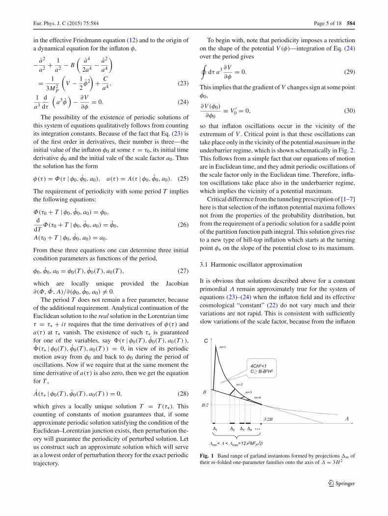


![arXiv · arXiv:1002.1416v3 [astro-ph.CO] 4 Jun 2010 Primordial Non-Gaussianities from Inflation Models Xingang Chen Center for Theoretical Cosmology, Department of Applied Mathematics](https://static.documents.pub/doc/80x56/5fce83e2111fdf56dc3a311d/arxiv-arxiv10021416v3-astro-phco-4-jun-2010-primordial-non-gaussianities-from.jpg)


