183
Orthogonality and Hermitian Analysis John P. D’Angelo Dept. of Mathematics, Univ. of Illinois, 1409 W. Green St., Ur- bana IL 61801 E-mail address : [email protected]
Orthogonality and Hermitian Analysis
John P. D’Angelo
Dept. of Mathematics, Univ. of Illinois, 1409 W. Green St., Ur-bana IL 61801
E-mail address: [email protected]
c©2012 by John P. D’Angelo

Contents
Chapter 1. Introduction to Fourier series 71. Introduction 72. A famous series 73. Trigonometric polynomials 104. Constant coefficient differential equations 145. The wave equation for a vibrating string 206. Solving the wave equation via exponentiation 227. Integrals 238. Approximate identities 259. Definition of Fourier series 2910. Summability methods 3211. The Laplace equation 3712. Uniqueness of Fourier coefficients for continuous functions 4113. Inequalities 43
Chapter 2. Hilbert spaces 471. Introduction 472. Norms and inner products 473. Subspaces and linear maps 524. Orthogonality 545. Orthonormal expansion 586. Polarization 607. Adjoints and unitary operators 628. A return to Fourier series 649. Bernstein’s theorem 6610. Compact Hermitian operators 6811. Sturm-Liouville theory 7312. Generating functions and orthonormal systems 8313. Spherical harmonics 87
Chapter 3. Fourier transform on R 931. Introduction 932. The Schwartz space 943. The dual space 974. Convolutions 1005. Plancherel theorem 1016. Heisenberg uncertainty principle 1027. Differential equations 1038. Pseudo-differential operators 1059. Hermite polynomials 107
3

4 CONTENTS
10. More on Sobolev spaces 10811. Inequalities 110
Chapter 4. Geometric considerations 1151. The isoperimetric inequality 1152. Elementary L2 inequalities 1183. Unitary groups 1254. Proper mappings 1305. Vector fields and differential forms 1366. Differential forms of higher degree 1407. Volumes of parametrized sets 1458. Volume computations 1499. Inequalities 15410. CR Geometry 15911. Positivity conditions for Hermitian polynomials 161
Chapter 5. Appendix 1651. The real and complex number systems 1652. Metric spaces 1683. Integrals 1714. Exponentials and trig functions 1735. Complex analytic functions 1746. Probability 175
Chapter 6. References 179
Index 181
CONTENTS 5
Preface
This book aims both to synthesize much of undergraduate mathematics andto introduce research topics in geometric aspects of complex analysis in severalvariables. The topics all relate to orthogonality, real analysis, elementary complexvariables, and linear algebra. I call the blend Hermitian analysis. The book devel-oped from my teaching experiences over the years and specifically from Math 428,a capstone Honors course taught in Spring 2013 at the University of Illinois. Manyof the students in Math 428 had taken honors courses in analysis, linear algebra,and beginning abstract algebra. They knew differential forms and Stokes’ theo-rem. Other students were strong in engineering, with less rigorous mathematicaltraining, but with a strong sense of how these ideas get used in applications.
Rather than repeating and reorganizing various parts of mathematics, thecourse began with Fourier series, a new topic for many of the students. Developingsome of this remarkable subject and related parts of analysis allows the synthesisof calculus, elementary real and complex analysis, and algebra. Proper mappings,unitary groups, complex vector fields, and differential forms eventually join thismotley crew. Orthogonality and Hermitian analysis unify these topics.
The book includes numerous examples and more than two-hundred exercises.These exercises sometimes appear, with a purpose, in the middle of a section. Thereader should stop reading and start computing.
Chapter 1 begins by considering the conditionally convergent series∑∞n=1
sin(nx)n .
We verify its convergence using summation by parts, which we discuss in some de-tail. We then review constant coefficient ordinary differential equations, the expo-nentiation of matrices, and the wave equation for a vibrating string. These topicsmotivate our development of Fourier series. We prove the Riesz-Fejer theorem char-acterizing non-negative trig polynomials. We develop topics such as approximateidentities and summability methods, enabling us to conclude the discussion on the
series∑∞n=1
sin(nx)n . The chapter closes with two proofs of Hilbert’s inequality.
Chapter 2 discusses the basics of Hilbert space theory, motivated by orthonor-mal expansions, and includes the spectral theorem for compact Hermitian opera-tors. We return to Fourier series after these Hilbert space techniques have becomeavailable. We also consider Sturm-Liouville theory in order to provide additionalexamples of orthonormal systems. The exercises include problems on Legendrepolynomials, Hermite polynomials, and several other collections of special func-tions. The chapter ends with a section on spherical harmonics, whose purpose isto indicate one possible direction for Fourier analysis in higher dimensions. As awhole, this chapter links classical and modern analysis. It considerably expands thematerial on Hilbert spaces from my Carus monograph Inequalities From ComplexAnalysis. Various items here help the reader to think in a magical Hermitian way.Here are two specific examples:
• There exist linear transformations A,B on a real vector space satisfyingthe relationship A−1 + B−1 = (A + B)−1 if and only if the vector spaceadmits a complex structure.
• It is well known that a linear map on a complex space preserves innerproducts if and only it preserves norms. This fact epitomizes the polar-ization technique which regards a complex variable or vector z and itsconjugate z as independent objects.

6 CONTENTS
Chapter 3 considers the Fourier transform on the real line, partly to glimpsehigher mountains and partly to give a precise meaning to distributions. We alsobriefly discuss Sobolev spaces and pseudo-differential operators. This chapter in-cludes several standard inequalities (Young, Holder, Minkowski) from real analysis.Extending these ideas to higher dimensions would be natural, but since many bookstreat this material well, we head in a different direction. This chapter is thereforeshorter than the other chapters and it contains fewer interruptions.
Chapter 4, the heart of the book, considers geometric issues revolving aroundthe unit sphere in complex Euclidean space. We begin with Hurwitz’s proof (us-ing Fourier series) of the isoperimetric inequality for smooth curves. We proveWirtinger’s inequality in two ways. We continue with an inequality on the areas ofcomplex analytic images of the unit disk, which we also prove in two ways. One ofthese involves differential forms. This chapter therefore includes several sections onvector fields and differential forms, including the complex case. Other geometricconsiderations in higher dimensions include topics from my own research: finiteunitary groups, group-invariant mappings, and proper mappings between balls.We use the notion of orthogonal homogenization to prove a sharp inequality on thevolume of the images of the unit ball under certain polynomial mappings. This ma-terial naturally leads to the Cauchy-Riemann (CR) Geometry of the unit sphere.The chapter closes with a brief discussion of positivity conditions for Hermitianpolynomials, connecting the work on proper mappings to an analogue of the Riesz-Fejer theorem in higher dimensions. Considerations of orthogonality and Hermitiangeometry weave all these topics into a coherent whole.
The prerequisites for reading the book include three semesters of calculus, linearalgebra, and basic real analysis. The reader needs some acquaintance with complexnumbers but does not require all of the material in the standard course. Theappendix summarizes the prerequisites. We occasionally employ the notation ofLebesgue integration, but knowing measure theory is not a prerequisite for readingthis book. The large number of exercises, many developed specifically for this book,should be regarded as crucial. They link the abstract and the concrete.
I thank the Department of Mathematics at Illinois for allowing me to teachvarious Honors courses and in particular the one for which I used these notes. Iacknowledge various people for their insights into some of the mathematics here,provided in conversations, published writing, or e-mail correspondences. Such peo-ple include Steve Bradlow, David Catlin, Geir Dullerud, Ed Dunne, Charlie Epstein,Burak Erdogan, Jerry Folland, Jen Halfpap, Zhenghui Huo, Robert Kaufman, RickLaugesen, Jeff McNeal, Tom Nevins, Mike Stone, Emil Straube, Jeremy Tyson,Bob Vanderbei, and others, including several unnamed reviewers.
I also thank Charlie Epstein and Steve Krantz for encouraging me to write abook for the Birkhauser Cornerstone Series. I much appreciate the efforts of KateGhezzi, Associate Editor of Birkhauser Science, who guided the evolution of myfirst draft into this book. I thank Carol Baxter of the Mathematical Association ofAmerica for granting me permission to incorporate some of the material from Chap-ter 2 of my Carus monograph Inequalities From Complex Analysis. I acknowledgeJimmy Shan for helping prepare pictures and solving many of the exercises.
I thank my wife Annette and our four children for their love.I acknowledge support from NSF grant DMS-1066177 and from the Kenneth
D. Schmidt Professorial Scholar award from the University of Illinois.

CHAPTER 1
Introduction to Fourier series
1. Introduction
We start the book by considering the series∑∞n=1
sin(nx)n , a nice example of a
Fourier series. This series converges for all real numbers x, but the issue of con-vergence is delicate. We introduce summation by parts as a tool for handling someconditionally convergent series of this sort. After verifying convergence, but beforefinding the limit, we pause to introduce and discuss several elementary differentialequations. This material also leads to Fourier series. We include the exponentiationof matrices here. The reader will observe these diverse topics begin being woveninto a coherent whole.
After these motivational matters, we introduce the fundamental issues con-cerning the Fourier series of Riemann integrable functions on the circle. We definetrigonometric polynomials, Fourier series, approximate identities, Cesaro and Abelsummability, and related topics enabling us to get some understanding of the con-vergence of Fourier series. We show how to use Fourier series to establish someinteresting inequalities.
In Chapter 2 we develop the theory of Hilbert spaces, which greatly clarifiesthe subject of Fourier series. We prove additional results about Fourier series there,after we know enough about Hilbert spaces. The manner in which concrete andabstract mathematics inform each other is truly inspiring.
2. A famous series
Consider the infinite series∑∞n=1
sin(nx)n . This sum provides an example of a
Fourier series, a term we will define precisely a bit later. Our first agenda item isto show that this series converges for all real x. After developing a bit more theory,we determine the sum for each x; the result defines the famous sawtooth function.
Let an be a sequence of (real or) complex numbers. We say that∑∞n=1 an
converges to L if
limN→∞
N∑n=1
an = L.
We say that∑∞n=1 an converges absolutely if
∑∞n=1 |an| converges. In case
∑an con-
verges, but does not converge absolutely, we say that∑an converges conditionally
or is conditionally convergent. Note that absolute convergence implies convergence,but that the converse fails. See for example Corollary 2.3. See the exercises forsubtleties arising when considering conditionally convergent series.
The expression AN =∑Nn=1 an is called the N -th partial sum. In this section
we will consider two sequences an and bn. We write their partial sums, usingcapital letters, as AN and BN . We regard the sequence of partial sums as an
7
8 1. INTRODUCTION TO FOURIER SERIES
analogue of the integral of the sequence of terms. Note that we can recover theterms from the partial sums because an = An −An−1, and we regard the sequencean of terms as an analogue of the derivative of the sequence of partial sums. Thenext result is extremely useful in analyzing conditionally convergent series. Onecan remember it by analogy with the integration by parts formula∫
aB′ = aB −∫a′B. (1)
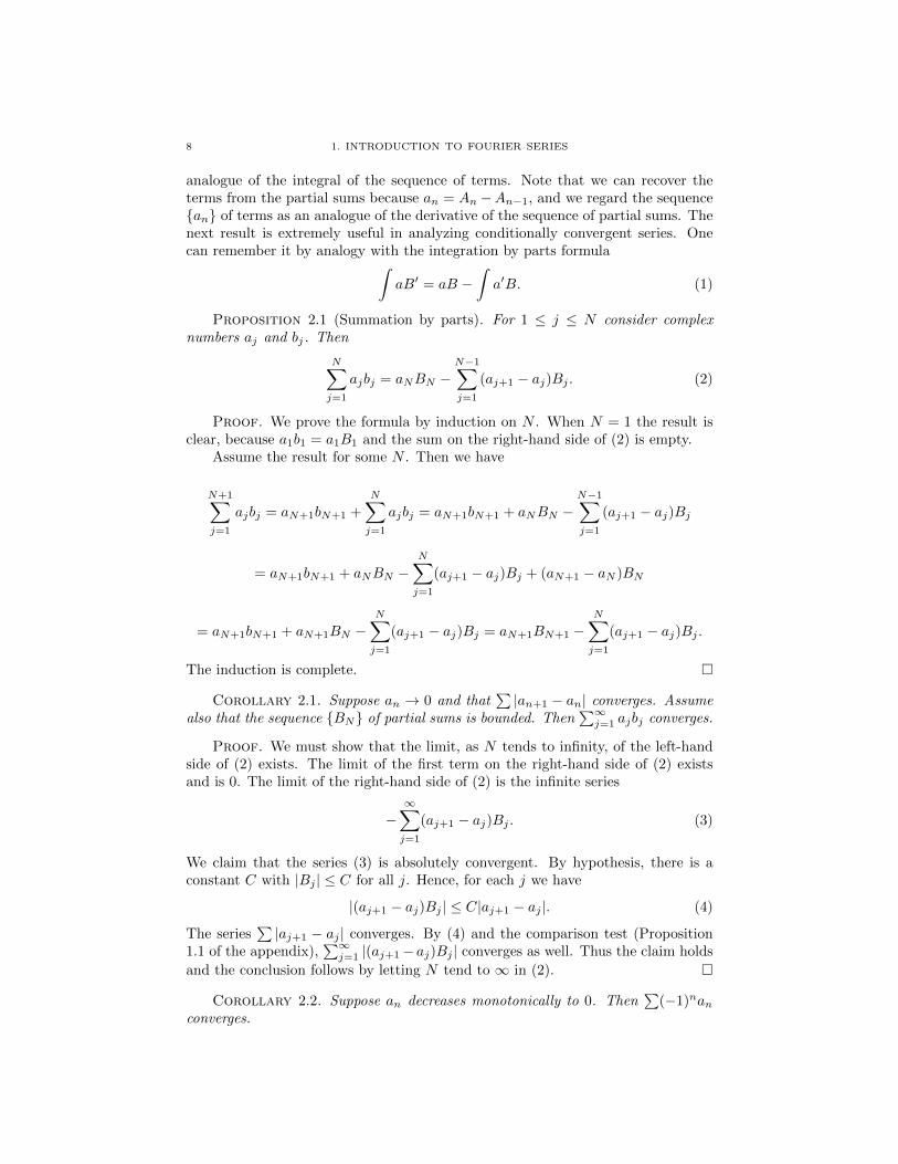
Proposition 2.1 (Summation by parts). For 1 ≤ j ≤ N consider complexnumbers aj and bj. Then
N∑j=1
ajbj = aNBN −N−1∑j=1
(aj+1 − aj)Bj . (2)
Proof. We prove the formula by induction on N . When N = 1 the result isclear, because a1b1 = a1B1 and the sum on the right-hand side of (2) is empty.
Assume the result for some N . Then we have
N+1∑j=1
ajbj = aN+1bN+1 +
N∑j=1
ajbj = aN+1bN+1 + aNBN −N−1∑j=1
(aj+1 − aj)Bj
= aN+1bN+1 + aNBN −N∑j=1
(aj+1 − aj)Bj + (aN+1 − aN )BN
= aN+1bN+1 + aN+1BN −N∑j=1
(aj+1 − aj)Bj = aN+1BN+1 −N∑j=1
(aj+1 − aj)Bj .
The induction is complete.
Corollary 2.1. Suppose an → 0 and that∑|an+1 − an| converges. Assume
also that the sequence BN of partial sums is bounded. Then∑∞j=1 ajbj converges.
Proof. We must show that the limit, as N tends to infinity, of the left-handside of (2) exists. The limit of the first term on the right-hand side of (2) existsand is 0. The limit of the right-hand side of (2) is the infinite series
−∞∑j=1
(aj+1 − aj)Bj . (3)
We claim that the series (3) is absolutely convergent. By hypothesis, there is aconstant C with |Bj | ≤ C for all j. Hence, for each j we have
|(aj+1 − aj)Bj | ≤ C|aj+1 − aj |. (4)
The series∑|aj+1 − aj | converges. By (4) and the comparison test (Proposition
1.1 of the appendix),∑∞j=1 |(aj+1− aj)Bj | converges as well. Thus the claim holds
and the conclusion follows by letting N tend to ∞ in (2).
Corollary 2.2. Suppose an decreases monotonically to 0. Then∑
(−1)nanconverges.
2. A FAMOUS SERIES 9
Proof. Put bn = (−1)n. Then |BN | ≤ 1 for all N . Since an+1 ≤ an for all n,
N∑j=1
|aj+1 − aj | =N∑j=1
(aj − aj+1) = a1 − aN+1.
Since aN+1 tends to 0, we have a convergent telescoping series. Thus Corollary 2.1applies.
Corollary 2.3.∑∞n=1
(−1)n
n converges.
Proof. Put an = 1n and bn = (−1)n. Corollary 2.2 applies.
Proposition 2.2.∑∞n=1
sin(nx)n converges for all real x.
Proof. Let an = 1n and let bn = sin(nx). First suppose x is an integer multiple
of π. Then bn = 0 for all n and the series converges to 0. Otherwise, suppose x isnot a multiple of π; hence eix 6= 1. We then claim that BN is bounded. In the next
section, for complex z we define sin(z) by eiz−e−iz2i and we justify this definition.
Using it we have
bn = sin(nx) =einx − e−inx
2i.
Since we are assuming eix 6= 1, the sum∑Nn=1 e
inx is a finite geometric serieswhich we can compute explicitly. We get
N∑n=1
einx = eix1− eiNx
1− eix. (5)
The right-hand side of (5) has absolute value at most 2|1−eix| and hence the left-
hand side of (5) is bounded independently of N . The same holds for∑Nn=1 e
−inx.Thus BN is bounded. The proposition now follows by Corollary 2.1.
Remark 2.1. The partial sums BN depend on x. We will see later why thelimit function fails to be continuous in x.
Remark 2.2. The definition of convergence of a series involves the partial sums.Other summability methods will arise soon. For now we note that conditionallyconvergent series are quite subtle. For example, in Exercise 2.1 you are asked toverify Riemann’s remark that the sum of a conditionally convergent series dependsin a striking way on the order in which the terms are added. Such a reordered seriesis called a rearrangement of the given series.
Exercise 2.1. Let∑an be a conditionally convergent series of real numbers.
Given any real number L (or ∞), prove that there is a rearrangement of∑an
that converges to L (or diverges). (Harder) Determine and prove a correspondingstatement if the an are allowed to be complex. (Hint: For some choices of complexnumbers an, not all complex L are possible as limits of rearranged sums. If, forexample, all the an are purely imaginary, then the rearranged sum must be purelyimaginary. Figure out all possible alternatives.)
Exercise 2.2. Show that∑∞n=2
sin(nx)log(n) and, (for α > 0),
∑∞n=1
sin(nx)nα con-
verge.

10 1. INTRODUCTION TO FOURIER SERIES
Exercise 2.3. Suppose that∑cj converges and that limn ncn = 0. Determine
∞∑n=1
n(cn+1 − cn).
Exercise 2.4. Find a sequence of complex numbers such that∑an converges
but∑
(an)3 diverges.
Exercise 2.5. This exercise has two parts.
(1) Assume that Cauchy sequences (see Section 1 of the Appendix) of realnumbers converge. Prove the following statement: if an is a sequenceof complex numbers and
∑∞n=1 |an| converges, then
∑∞n=1 an converges.
(2) Next, do not assume that Cauchy sequences of real numbers converge;instead assume that whenever
∑∞n=1 |an| converges, then
∑∞n=1 an con-
verges. Prove that Cauchy sequences of real (or complex) numbers con-verge.
Exercise 2.6. (Difficult) For 0 < x < 2π, show that∑∞n=0
cos(nx)log(n+2) converges
to a non-negative function. Suggestion: Sum by parts twice and find an explicit
formula for∑Nn=1
∑nk=1 cos(kx). If needed, look ahead to formula (49).
3. Trigonometric polynomials
We let S1 denote the unit circle in C. Our study of Fourier series involvesfunctions defined on the unit circle, although we sometimes work with functionsdefined on R, on the interval [−π, π], or on the interval [0, 2π]. In order that suchfunctions be defined on the unit circle, we must assume that they are periodic withperiod 2π, that is, f(x+ 2π) = f(x). The most obvious such functions are sine andcosine. We will often work instead with complex exponentials.
We therefore begin by defining, for z ∈ C,
ez =
∞∑n=0
zn
n!= limN→∞
N∑n=0
zn
n!. (6)
Using the ratio test, we see that the series in (6) converges absolutely for each z ∈ C.It converges uniformly on each closed ball in C. Hence the series defines a complexanalytic function of z whose derivative (which is also ez) is found by differentiatingterm-by-term. See the appendix for the definition of complex analytic function.
Note that e0 = 1. Also it follows from (6) that, for all complex numbers z andw, ez+w = ezew. (See Exercise 3.8.) From these facts we can also see for λ ∈ Cthat d
dz eλz = λeλz. Since complex conjugation is continuous, we also have ez = ez
for all z. (Continuity is used in passing from the partial sum in (6) to the infiniteseries.) Hence when t is real we see that e−it is the conjugate of eit. Therefore
|eit|2 = eite−it = e0 = 1
and hence eit lies on the unit circle. All trigonometric identities follow from thedefinition of the exponential function. The link to trigonometry (trig) comes fromthe definitions of sine and cosine for a complex variable z:
cos(z) =eiz + e−iz
2(7)

3. TRIGONOMETRIC POLYNOMIALS 11
sin(z) =eiz − e−iz
2i. (8)
We obtain eit = cos(t) + isin(t). In particular, when t is real, cos(t) is the real partof eit and sin(t) is the imaginary part of eit. Hence cos(t) and sin(t) have theirusual meanings when t is real.
Although we started the book with the series∑ sin(nx)
n , we prefer using complexexponentials instead of cosines and sines to express our ideas and formulas.
Definition 3.1. A complex-valued function on the circle is called a trigono-metric polynomial or trig polynomial if there are complex constants cj such that
f(θ) =
N∑j=−N
cjeijθ.
It is of degree N if CN or C−N 6= 0. The complex numbers cj are called the(Fourier) coefficients of f .
Lemma 3.1. A trig polynomial f is the zero function if and only if all itscoefficients vanish.
Proof. If all the coefficients vanish, then f is the zero function. The converseis less trivial. We can recover the coefficients cj of a trig polynomial by integration:
cj =1
2π
∫ 2π
0
f(θ)e−ijθdθ. (9)
If f(θ) = 0 for all θ, then each of these integrals vanishes and the converse assertionfollows.
See Theorem 12.1 for an important generalization. Lemma 3.1 has a geometricinterpretation, which we will develop and generalize in Chapter 2. The functionsx→ einx for −N ≤ n ≤ N form an orthonormal basis for the (2N +1)-dimensionalvector space of trig polynomials of degree at most N . The lemma states that f isthe zero vector if and only if all its components with respect to this basis are 0.
We need the following result about real-valued trig polynomials. See Lemma9.1 for a generalization.
Lemma 3.2. A trig polynomial is real-valued if and only if cj = c−j for all j.
Proof. The trig polynomial is real valued if and only if f = f , which becomes
N∑j=−N
cjeijθ =
N∑j=−N
cje−ijθ. (10)
Replacing j by −j in the second sum in (10) shows that f is real-valued if and onlyif
N∑j=−N
cjeijθ =
N∑j=−N
cje−ijθ =
−N∑j=N
c−jeijθ =
N∑j=−N
c−jeijθ. (11)
The difference of the two far sides of (11) is the zero function; hence the conclusionfollows from Lemma 3.1.
We sometimes call this condition on the coefficients the palindrome property; itcharacterizes real-valued trig polynomials. Our next result, which is considerablymore difficult, characterizes non-negative trig polynomials.
12 1. INTRODUCTION TO FOURIER SERIES
Theorem 3.1 (Riesz-Fejer 1916). Let f be a trig polynomial with f(θ) ≥ 0 forall θ. Then there is a complex polynomial p(z) such that f(θ) = |p(eiθ)|2.
Proof. Assume f is of degree d and write
f(θ) =
d∑j=−d
cjeijθ,
where c−j = cj since f is real-valued. Note also that c−d 6= 0. Define a polynomialq in one complex variable by
q(z) = zdd∑
j=−d
cjzj . (12)
Let ξ1, ..., ξ2d be the roots of q, repeated if necessary. We claim that the realityof f , or equivalently the palindrome property, implies that if ξ is a root of q, then(ξ)−1 also is a root of q. This point is called the reflection of ξ in the circle. SeeFigure 1. Because 0 is not a root, the claim follows from the formula
q(z) = z2d q((z)−1). (13)
To check (13), we use (12) and the palindrome property. Also, we replace −j by jin the sum to get
z2d q((z)−1) = zd∑
cj(1
z)j = zd
∑cjz−j = zd
∑c−jz
j = zd∑
cjzj = q(z).
Thus (13) holds. It also follows that each root on the circle must occur with evenmultiplicity. Thus the roots of q occur in pairs, symmetric with respect to the unitcircle.
By the Fundamental Theorem of Algebra, we may factor the polynomial q intolinear factors. For z on the circle we can replace the factor z − (ξ)−1 with
1
z− 1
ξ=ξ − zzξ
.
Let p(z) = C∏dj=1(z − ξj). Here we use all the roots in the unit disk and half
of those where |ξj | = 1. Note that |q| = |p|2 on the circle. Since f ≥ 0 on the circle,we obtain
f(θ) = |f(θ)| = |q(eiθ)| = |p(eiθ)|2.
Exercise 3.1. Put f(θ) = 1 + a cos(θ). Note that f ≥ 0 if and only if |a| ≤ 1.In this case find p such that |p(z)|2 = f(z) on the circle.
Exercise 3.2. Put f(θ) = 1 + a cos(θ) + b cos(2θ). Find the condition ona, b for f ≥ 0. Carefully graph the set of (a, b) for which f ≥ 0. Find p such thatf = |p|2 on the circle. Suggestion: To determine the condition on a, b, rewrite f asa polynomial in x on the interval [−1, 1].
Exercise 3.3. Find a polynomial p such that |p(eiθ)|2 = 4 − 4sin2(θ). (Theroots of p lie on the unit circle, illustrating part of the proof of Theorem 3.1.)

3. TRIGONOMETRIC POLYNOMIALS 13
Ξ
1Ξ
-1.0 -0.5 0.5 1.0 1.5
-1.0
-0.5
0.5
1.0
1.5
Figure 1. Reflection in the circle
In anticipation of later work, we introduce Hermitian symmetry and rephrasethe Riesz-Fejer theorem in this language.
Definition 3.2. Let R(z, w) be a polynomial in the two complex variables z
and w. R is called Hermitian symmetric if R(z, w) = R(w, z) for all z and w.
The next lemma characterizes Hermitian symmetric polynomials.
Lemma 3.3. The following statements about a polynomial in two complex vari-ables are equivalent:
(1) R is Hermitian symmetric.(2) For all z, R(z, z) is real.(3) R(z, w) =
∑a,b cabz
awb where cab = cba for all a, b.
Proof. Left to the reader.
The next result, together with various generalizations, justifies regarding z andits conjugate z as independent variables. When a polynomial identity in z and zholds for all z, it holds when we vary z and z separately.
Lemma 3.4 (Polarization). Let R be a Hermitian symmetric polynomial. IfR(z, z) = 0 for all z, then R(z, w) = 0 for all z and w.
Proof. Write z = |z|eiθ. Plugging into the third item from Lemma 3.3, weare given ∑
cab|z|a+bei(a−b)θ = 0
for all |z| and for all θ. Put k = a − b, which can be positive, negative, or 0. ByLemma 3.1, the coefficient of each eikθ is 0. Thus, for all k and z
|z|k∑
c(b+k)b|z|2b = 0. (14)
After dividing by |z|k, for each k (14) defines a polynomial in |z|2 that is identically0. Hence each coefficient c(b+k)b vanishes and R is the zero polynomial.
Example 3.1. Note that |z+ i|2 = |z|2− iz+ iz+ 1. Polarization implies that(z + i)(w− i) = zw− iz + iw+ 1 for all z and w. We could also replace w with w.
14 1. INTRODUCTION TO FOURIER SERIES
Remark 3.1. We can restate the Riesz-Fejer Theorem in terms of Hermitiansymmetric polynomials: If r is Hermitian symmetric and non-negative on the cir-cle, then r(z, z) = |p(z)|2 there. (Note that there are many Hermitian symmetricpolynomials agreeing with a given trig polynomial on the circle.) The higher dimen-sional analogue of the Riesz-Fejer theorem uses Hermitian symmetric polynomials.See Theorem 11.2 of Chapter 4 and [D1].
Exercise 3.4. Prove Lemma 3.3.
Exercise 3.5. Verify the second sentence of Remark 3.1.
Exercise 3.6. Explain why the factor z2d appears in (13).
Exercise 3.7. Assume a ∈ R, b ∈ C, and c > 0. Find the minimum of theHermitian polynomial R:
R(t, t) = a+ bt+ bt+ c|t|2.
Compare with the proof of the Cauchy-Schwarz inequality, Theorem 2.1 ofChapter 2.
Exercise 3.8. Prove that ez+w = ezew.
Exercise 3.9. Simplify the expression∑kj=1 sin((2j − 1)x).
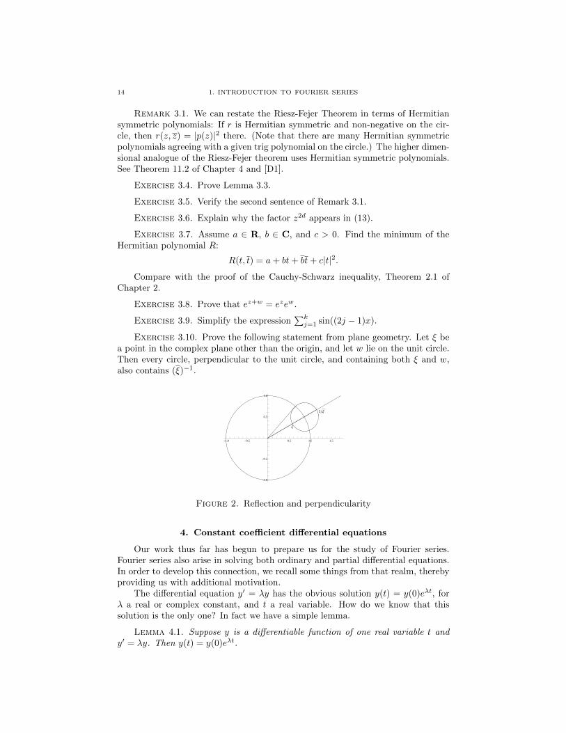
Exercise 3.10. Prove the following statement from plane geometry. Let ξ bea point in the complex plane other than the origin, and let w lie on the unit circle.Then every circle, perpendicular to the unit circle, and containing both ξ and w,also contains (ξ)−1.
Ξ
1 Ξ
-1.0 -0.5 0.5 1.0 1.5
-1.0
-0.5
0.5
1.0
Figure 2. Reflection and perpendicularity
4. Constant coefficient differential equations
Our work thus far has begun to prepare us for the study of Fourier series.Fourier series also arise in solving both ordinary and partial differential equations.In order to develop this connection, we recall some things from that realm, therebyproviding us with additional motivation.
The differential equation y′ = λy has the obvious solution y(t) = y(0)eλt, forλ a real or complex constant, and t a real variable. How do we know that thissolution is the only one? In fact we have a simple lemma.
Lemma 4.1. Suppose y is a differentiable function of one real variable t andy′ = λy. Then y(t) = y(0)eλt.

4. CONSTANT COEFFICIENT DIFFERENTIAL EQUATIONS 15
Proof. Let y be differentiable with y′ = λy. Put f(t) = e−λty(t). Theproduct rule for derivatives gives f ′(t) = e−λt(−λy(t)+y′(t)) = 0. The mean-valuetheorem from calculus guarantees that the only solution to f ′ = 0 is a constant c.Hence e−λty(t) is a constant c, which must be y(0), and y(t) = y(0)eλt.
This result generalizes to constant coefficient equations of higher order; seeTheorem 4.1. Such equations reduce to first order systems. Here is the simple idea.Given a k-times differentiable function y of one variable, we form the vector-valuedfunction Y : R→ Rk+1 as follows:
Y (t) =
y(t)y′(t)...
y(k)(t)
. (15)
The initial vector Y (0) in (15) tells us the values for y(0), y′(0), . . . , y(k)(0).Consider the differential equation y(m) = c0y+ c1y
′+ ...+ cm−1y(m−1). Here y
is assumed to be an m-times differentiable function of one variable t, and each cjis a constant. Put k = m− 1 in (15). Define an m-by-m matrix A as follows:
A =
0 1 0 ... 00 0 1 ... 0... ... ... 1 00 0 ... 0 1c0 c1 c2 ... cm−1
(16)
Consider the matrix product AY and the equation Y ′ = AY . The matrix Ahas been constructed such that the first m − 1 rows of this equation tell us thatddty
(j) = y(j+1), and the last row tells us that y(m) =∑cjy
(j). The equation
y(m) = c0y + c1y′ + ...+ cm−1y
(m−1)
is therefore equivalent to the first-order matrix equation Y ′ = AY . In analogy withLemma 4.1, we solve this system by exponentiating the matrix A.
Let Mν denote a sequence of matrices of complex numbers. We say that Mν
converges to M if each entry of Mν converges to the corresponding entry of M .Let M be a square matrix, say n-by-n, of real or complex numbers. We define
eM , the exponential of M , by the series
eM =
∞∑k=0
Mk
k!= limN→∞
N∑k=0
Mk
k!. (17)
It is not difficult to show that this series converges and also, when MK = KM , thateM+K = eMeK . Note also that e0 = I, where I denotes the identity matrix. As aconsequence of these facts, for each M the matrix eM is invertible and e−M is itsinverse. It is also easy to show that MeM = eMM , that is, M and its exponentialeM commute. We also note that eAt is differentiable and d
dteAt = AeAt.
Exercise 4.1. Prove that the series in (17) converges for each square matrixof complex numbers. Suggestion. Use the Weierstrass M -test to show that eachentry converges.
Exercise 4.2. If B is invertible, prove for each positive integer k that
(BMB−1)k = BMkB−1.

16 1. INTRODUCTION TO FOURIER SERIES
Exercise 4.3. If B is invertible, prove that BeMB−1 = eBMB−1
.
Exercise 4.4. Find a simple expression for det(eM ) in terms of a trace.
A simple generalization of Lemma 4.1 enables us to solve constant coefficientordinary differential equations (ODE)s of higher order m. As mentioned above, theinitial vector Y (0) provides m pieces of information.
Theorem 4.1. Suppose y : R → R is m times differentiable and there areconstants cj such that
y(m) =
m−1∑j=0
cjy(j). (18)
Define Y as in (15) and A as in (16) above. Then Y (t) = eAtY (0), and y(t) is thefirst component of eAtY (0).
Proof. Suppose Y is a solution. Differentiating e−AtY (t) gives
d
dt
(e−AtY (t)
)= e−At(Y ′(t)−AY (t)). (19)
Since y satisfies (18), the expression in (19) is the zero element of Rm. Hencee−AtY (t) is a constant element of Rm and the result follows.
In order to apply this result we need a good way to exponentiate matrices(linear mappings). Let A : Cn → Cn be a linear transformation. Recall that λis called an eigenvalue for A if there is a non-zero vector v such that Av = λv.The vector v is called an eigenvector corresponding to λ. One sometimes findseigenvalues by finding the roots of the polynomial det(A − λI). We note that theroots of this equation can be complex even if A is real and we consider A to be anoperator on Rn.
In order to study the exponentiation of A, we first assume that A has n distincteigenvalues. By linear algebra, shown below, there is an invertible matrix P and adiagonal matrix D such that A = PDP−1. Since (PDP−1)k = PDkP−1 for eachk, it follows that
eA = ePDP−1
= PeDP−1. (20)
It is easy to find eD; it is the diagonal matrix whose eigenvalues (the diagonalelements in this case) are the exponentials of the eigenvalues of D.
We recall how to find P . Given A with distinct eigenvalues, for each eigenvalueλj we find an eigenvector vj . Thus vj is a non-zero vector and A(vj) = λjvj . Thenwe may take P to be the matrix whose columns are these eigenvectors. We includethe simple proof. First, the eigenvectors form a basis of Cn because the eigenvaluesare distinct.
Let ej be the j-th standard basis element of Rn. Let D be the diagonal matrixwith D(ej) = λjej . By definition, P (ej) = vj . Therefore
PDP−1(vj) = PD(ej) = P (λjej) = λjP (ej) = λjvj = A(vj). (21)
By (21), A and PDP−1 agree on a basis, and hence they define the same linearmapping. Thus A = PDP−1.
We apply this reasoning to solve the general second order constant coefficienthomogeneous differential equation y′′ = b1y
′ + b0y. Let λ1 and λ2 be the roots ofthe polynomial λ2 − b1λ− b0 = 0.

4. CONSTANT COEFFICIENT DIFFERENTIAL EQUATIONS 17
Corollary 4.1. Assume y : R→ C is twice differentiable, and
y′′ − (λ1 + λ2)y′ + λ1λ2y = 0 (22)
for complex numbers λ1 and λ2. If λ1 6= λ2, then there are complex constants c1and c2 such that
y(t) = c1eλ1t + c2e
λ2t. (23)
In case λ1 = λ2, the answer is given by
y(t) = eλty(0) + teλt(y′(0)− λy(0)).
Proof. Here the matrix A is given by(0 1
−λ1λ2 λ1 + λ2
). (24)
Its eigenvalues are λ1 and λ2. When λ1 6= λ2, we obtain eAt by the formula
eAt = PeDtP−1,
where D is the diagonal matrix with eigenvalues λ1 and λ2, and P is the change ofbasis matrix. Here eDt is diagonal with eigenvalues eλ1t and eλ2t:
eAt =1
λ2 − λ1
(1 1λ1 λ2
)(eλ1t 0
0 eλ2t
)(λ2 −1−λ1 1
)The factor 1
λ2−λ1on the outside arises in finding P−1. Performing the indicated
matrix multiplications, introducing the values of y and y′ at 0, and doing sometedious work gives
y(t) =(λ2e
λ1t − λ1eλ2t)y(0) + (eλ2t − eλ1t)y′(0)
λ2 − λ1. (25)
Formula (23) is a relabeling of (25). An ancillary advantage of writing the answerin the form (25) is that we can take the limit as λ2 tends to λ1 and obtain thesolution in case these numbers are equal; write λ = λ1 = λ2 in this case. The result(See Exercise 4.5) is
y(t) = eλty(0) + teλt(y′(0)− λy(0)). (26)
A special case of this corollary arises often. For c real but not 0, the solutionsto the differential equation y′′ = cy are (complex) exponentials. The behavior ofthe solutions depends in a significant way on the sign of c. When c = k2 > 0, thesolutions are linear combinations of e±kt. Such exponentials either decay or growat infinity. When c = −k2, however, the solutions are linear combinations of e±ikt,which we express instead in terms of sines and cosines. In this case the solutionsoscillate.
Exercise 4.5. Show that (25) implies (26).
The assumption that A has distinct eigenvalues is used only to find eAt easily.Even when A has repeated eigenvalues and the eigenvectors do not span the space,the general solution to Y ′ = AY remains Y (t) = eAtY (0). The Jordan normal formallows us to write A = P (D+N)P−1, where D is diagonal and N is nilpotent of aparticular form. If the eigenvectors do not span, then N is not 0. It is often easier
18 1. INTRODUCTION TO FOURIER SERIES
in practice to exponentiate A by using the ideas of differential equations ratherthan by using linear algebra. The proof from Exercise 4.5 that (25) implies (26)nicely illustrates the general idea. See also Exercises 4.9 and 4.12.
Exercise 4.6. Explain how to find eAt when the eigenvectors of A do not spanthe full space. In particular find eA if
A =
(λ 10 λ
).
Exercise 4.7. Give an example of two-by-two matrices A and B such thateAeB 6= eA+B .
4.1. Inhomogeneous linear differential equations. We also wish to solveinhomogeneous differential equations. To do so, we introduce natural notation.Let p(z) = zm −
∑m−1j=0 cjz
j be a monic polynomial of degree m. Let D represent
the operation of differentiation with respect to x. We define the operator p(D) byformally substituting Dj for zj .
In Theorem 4.1, we solved the equation p(D)y = 0. In applications, however,one often needs to solve the equation p(D)y = f for a given forcing function f . Forexample, one might turn on a switch at a given time x0, in which case f could bethe function that is 0 for x < x0 and is 1 for x ≥ x0.
Since the operator p(D) is linear, the general solution to p(D)y = f can bewritten y = y0 + y∗, where y0 is a solution to the equation p(D)y = 0 and y∗ isany particular solution to p(D)y∗ = f . We already know how to find all solutionsto p(D)(y0) = 0. Thus we need only to find one particular solution. To do so,we proceed as follows. Using the fundamental theorem of algebra, we factor thepolynomial p:
p(z) =
m∏k=1
(z − λk),
where the λk can be repeated if necessary.When m = 1 we can solve the equation (D − λ1)g1 = f by the following
method. We suppose that g1(x) = c(x)eλ1x for some differentiable function c.Applying D − λ1 to g1 we get
(D − λ1)g1 = (c′(x) + c(x)λ1)eλ1x − λ1c(x)eλ1x = c′(x)eλ1x = f(x).
For an arbitrary real number a (often it is useful to take a = ±∞), we obtain
c(x) =
∫ x
a
f(t)e−λ1tdt.
This formula yields the particular solution g1 defined by
g1(x) = eλ1x
∫ x
a
e−λ1tf(t)dt,
and amounts to finding the inverse of the operator D − λ1.The case m > 1 follows easily from the special case. We solve the equation
(D − λ1)(D − λ2) . . . (D − λm)(y) = f
by solving (D − λ1)g1 = f , and then for j > 1 solving (D − λj)gj = gj−1. Thefunction y = gm then solves the equation p(D)y = f .
4. CONSTANT COEFFICIENT DIFFERENTIAL EQUATIONS 19
Remark 4.1. Why do we start with the term on the far left? The reason isthat the inverse of the composition (D−λ1)(D−λ2) . . . (D−λn) is the compositionof the inverses in the reverse order. To take off our socks, we must first take off ourshoes.
Example 4.1. We solve (D − 5)(D − 3)y = ex. First we solve (D − 5)g = ex,obtaining
g(x) = e5x
∫ x
∞ete−5tdt =
−1
4ex.
Then we solve (D − 3)h = −14 e
x to get
h(x) = e3x
∫ x
∞
−1
4ete−3tdt =
1
8ex.
The general solution to the equation is c1e5x + c2e
3x + 18ex, where c1 and c2 are
constants. We put a =∞ because e−λt vanishes at ∞ if λ > 0.
Exercise 4.8. Find all solutions to (D2 +m2)y = ex.
Exercise 4.9. Solve (D− λ)y = eλx. Use the result to solve (D− λ)2(y) = 0.Compare the method with the result from Corollary 4.1, when λ1 = λ2.
Exercise 4.10. Find a particular solution to (D − 5)y = 1− 75x2.
Exercise 4.11. We wish to find a particular solution to (D − λ)y = g, wheng is a polynomial of degree m. Identify the coefficients of g as a vector in Cm+1.Assuming λ 6= 0, show that there is a unique particular solution y that is a poly-nomial of degree m. Write explicitly the matrix of the linear transformation thatsends y to g and note that it is invertible. Explain precisely what happens whenλ = 0.
Exercise 4.12. Consider the equation (D − λ)my = 0. Prove by inductionthat xjeλx for 0 ≤ j ≤ m− 1 form a linearly independent set of solutions.
We conclude this section with some elementary remarks about solving systemsof linear equations in finitely many variables; these remarks inform to a large degreethe methods used throughout this book. The logical development enabling thepassage from linear algebra to solving linear differential equations was one of thegreat achievements of 19-th century mathematics.
Consider a system of k linear equations in n real variables. We regard thissystem as a linear equation Ly = w, where L : Rn → Rk. Things work out better(as we shall see) in terms of complex variables; thus we consider the linear equationLz = w, where now L : Cn → Ck. Let 〈z, ζ〉 denote the usual Hermitian Euclideaninner product on both the domain and target spaces. Let L∗ denote the adjoint ofL. The matrix representation of L∗ is the conjugate transpose of L. Then Lz = wimplies (for all ζ)
〈w, ζ〉 = 〈Lz, ζ〉 = 〈z, L∗ζ〉.In order that the equation Lz = w have a solution at all, the right-hand side wmust be orthogonal to the nullspace of L∗.
Consider the case where the number of equations equals the number of variables.Using eigenvalues and orthonormal expansion (to be developed in Chapter 2 forHilbert spaces), we can attempt to solve the equation Lz = w as follows. Underthe assumption that L = L∗, there is an orthonormal basis of Cn consisting of
20 1. INTRODUCTION TO FOURIER SERIES
eigenvectors φj with corresponding real eigenvalues λj . We can then write both zand w in terms of this basis, obtaining
w =∑〈w, φj〉φj
z =∑〈z, φj〉φj .
Equating Lz to w, we get∑〈z, φj〉λjφj =
∑〈w, φj〉φj .
Now equating coefficients yields
〈z, φj〉λj = 〈w, φj〉. (27)
If λj = 0, then w must be orthogonal to φj . If w satisfies this condition for allappropriate j, then we can solve Lz = w by division. On each eigenspace withλj 6= 0, we divide by λj to find 〈z, φj〉 and hence we find a solution z. The solutionis not unique in general; we can add to z any solution ζ to Lζ = 0. These ideasrecur throughout this book, both in the Fourier series setting and in differentialequations.
5. The wave equation for a vibrating string
The wave equation discussed in this section governs the motion of a vibratingstring. The solution of this equation naturally leads to Fourier series.
We are given a twice differentiable function u of two variables, x and t, with xrepresenting position and t representing time. Using subscripts for partial deriva-tives, the wave equation is
uxx =1
c2utt. (28)
Here c is a constant which equals the speed of propagation of the wave.Recall that a function is continuously differentiable if it is differentiable and its
derivative is continuous. It is twice continuously differentiable if it is twice differen-tiable and the second derivative is continuous. We have the following result aboutthe partial differential equation (28). After the proof we discuss the appropriateinitial conditions.
Theorem 5.1. Let u : R × R → R be twice continuously differentiable andsatisfy (28). Then there are twice continuously differentiable functions F and G(of one variable) such that
u(x, t) = F (x+ ct) +G(x− ct).
Proof. Motivated by writing α = x+ ct and β = x− ct,we define a functionφ by
φ(α, β) = u(α+ β
2,α− β
2c).
We compute second derivatives by the chain rule, obtaining
φαβ =d
dβφα =
d
dβ(ux2
+ut2c
) =uxx4− uxt
4c+utx4c− utt
4c2= 0. (29)
Note that we have used the equality of the mixed second partial derivatives uxt andutx. It follows that φα is independent of β, hence a function h of α alone. Integrating
5. THE WAVE EQUATION FOR A VIBRATING STRING 21
again, we see that φ is the integral F of this function h plus an integration constant,say G, which will depend on β. We obtain
u(x, t) = φ(α, β) = F (α) +G(β) = F (x+ ct) +G(x− ct). (30)
This problem becomes more realistic if x lies in a fixed interval and u satis-fies initial conditions. For convenience we let this interval be [0, π]. We can alsochoose units for time to make c = 1. The conditions u(0, t) = u(π, t) = 0 statethat the string is fixed at the points 0 and π. The initial conditions for time areu(x, 0) = f(x), and ut(x, 0) = g(x). The requirement u(x, 0) = f(x) means thatthe initial displacement curve of the string is defined by the equation y = f(x).The requirement on ut means that the string is given the initial velocity g(x).
Note that f and g are not the same functions as F and G from Theorem 5.1above. We can, however, easily express F and G in terms of f and g.
First we derive d’Alembert’s solution, Theorem 5.2. Then we attempt to solvethe wave equation by way of separation of variables. That method leads to a Fourierseries. In the next section we obtain the d’Alembert solution by regarding the waveequation as a constant coefficient ODE, and treating the second derivative operatorD2 as a number.
Theorem 5.2. Let u be twice continuously differentiable and satisfy uxx = utt,together with the initial conditions u(x, 0) = f(x) and ut(x, 0) = g(x). Then
u(x, t) =f(x+ t) + f(x− t)
2+
1
2
∫ x+t
x−tg(a)da. (31)
Proof. Using the F and G from Theorem 5.1, and assuming c = 1, we aregiven F +G = f and F ′ −G′ = g. Differentiating, we obtain the system(
1 11 −1
)(F ′
G′
)=
(f ′
g
). (32)
Solving (32) by linear algebra expresses F ′ and G′ in terms of f and g: we obtain
F ′ = f ′+g2 and G′ = f ′−g
2 . Integrating and using (30) with c = 1 yields (31).
We next attempt to solve the wave equation by separation of variables. Thestandard idea seeks a solution of the form u(x, t) = A(x)B(t). Differentiating andusing the equation uxx = utt leads to A′′(x)B(t) = A(x)B′′(t), and hence the
expressions A′′(x)A(x) and B′′(t)
B(t) are equal. Since one depends on x and the other on
t, each must be constant. Thus we have A′′(x) = ξA(x) and B′′(t) = ξB(t) whichwe solve as in Corollary 4.1. For each ξ we obtain solutions. If we insist thatthe solution is a wave, then we must have ξ < 0 (as the roots are then purelyimaginary). Thus
A(x) = a1sin(√|ξ|x) + a2cos(
√|ξ|x)
for constants a1, a2. If the solution satisfies the condition A(0) = 0, then a2 = 0. If
the solution also satisfies the condition A(π) = 0, then√|ξ| is an integer. Putting
this information together, we obtain a collection of solutions um indexed by theintegers:
um(x, t) = (dm1cos(mt) + dm2
sin(mt)) sin(mx),

22 1. INTRODUCTION TO FOURIER SERIES
for constants dm1and dm2
. Adding these solutions (the superposition of thesewaves) we are led to a candidate for the solution:
u(x, t) =
∞∑m=0
(dm1cos(mt) + dm2
sin(mt)) sin(mx).
Given u(x, 0) = f(x), we now wish to solve the equation (where dm = dm1)
f(x) =∑m
dmsin(mx). (33)
Again we encounter a series involving the terms sin(mx). At this stage, the basicquestion becomes, given a function f with f(0) = f(π) = 0, whether there areconstants such that (33) holds. We are thus asking whether a given function canbe represented as the superposition of (perhaps infinitely many) sine waves. Thissort of question arises throughout applied mathematics.
Exercise 5.1. Give an example of a function on the real line that is differen-tiable (at all points) but not continuously differentiable.
Exercise 5.2. Suppose a given function f can be written in the form (33),where the sum is either finite or converges uniformly. How can we determine theconstants dm? (We will solve this problem in Section 9.)
We conclude this section with a few remarks about the inhomogeneous waveequation. Suppose that an external force acts on the vibrating string. The waveequation (28) then becomes
uxx −1
c2utt = h(x, t) (∗)
for some function h determined by this force. Without loss of generality, we againassume that c = 1. We still have the initial conditions u(0, t) = u(π, t) = 0 as wellas u(x, 0) = f(x) and ut(x, 0) = g(x). We can approach this situation also by usingsine series. We presume that both u and h are given by sine series:
u(x, t) =∑
dm(t)sin(mx)
h(x, t) =∑
km(t)sin(mx).
Plugging into (*), we then obtain a family of second order constant coefficient ODErelating dm to km:
d′′m(t) +m2dm(t) = −km(t).
We can then solve these ODEs by the method described just before Remark 4.1.This discussion indicates the usefulness of expanding functions in series such as (33)or, more generally, as series of the form
∑n dne
inx.
6. Solving the wave equation via exponentiation
This section is not intended to be rigorous. Its purposes are to illuminateTheorem 5.2 and to glimpse some deeper ideas.
Consider the partial differential equation (PDE) on R×R given by uxx = uttwith initial conditions u(x, 0) = f(x) and ut(x, 0) = g(x). We regard it formally asa second order ordinary differential equation as follows:

7. INTEGRALS 23
(uu′
)′=
(u′
u′′
)=
(0 1D2 0
)(uu′
). (34)
Here D2 is the operator of differentiating twice with respect to x, but we treat itformally as a number. Using the method of Corollary 4.1, we see formally that theanswer is given by
(u(x, t)ut(x, t)
)= e
0 1D2 0
t(f(x)g(x)
)(35)
The eigenvalues of
(0 1D2 0
)are ±D and the change of basis matrix is given by
P =
(1 −1D D
).
Proceeding formally as if D were a nonzero number, we obtain by this method
u(x, t) =eDt + e−Dt
2f(x) +
eDt − e−Dt
2(D−1g)(x). (36)
We need to interpret the expressions e±Dt andD−1 in order for (36) to be useful.It is natural for D−1 to mean integration. We claim that eDtf(x) = f(x+ t). Wedo not attempt to prove the claim, as a rigorous discussion would take us far fromour aims, but we ask the reader to give a heuristic explanation in Exercise 6.1.The claim and (36) yield d’Alembert’s solution, the same answer we obtained inTheorem 5.2.
u(x, t) =f(x+ t) + f(x− t)
2+
1
2
∫ x+t
x−tg(u)du. (37)
Exercise 6.1. Give a suggestive argument why eDtf(x) = f(x+ t).
7. Integrals
We are now almost prepared to begin our study of Fourier series. In this sectionwe introduce some notation and say a few things about integration.
When we say that f is integrable on the circle, we mean that f is Riemann inte-grable on [0, 2π] there and that f(0) = f(2π). By definition, a Riemann integrablefunction must be bounded. Each continuous function is Riemann integrable, butthere exist Riemann integrable functions that are discontinuous at an infinite (butsmall, in the right sense) set of points.
Some readers may have seen the more general Lebesgue integral and measuretheory. We sometimes use notation and ideas usually introduced in that context.For example, we can define measure zero without defining measure. A subset S ofR has measure zero, if for every ε > 0, we can find a sequence In of intervalssuch that S is contained in the union of the In and the sum of the lengths of theIn is less than ε. A basic theorem we will neither prove nor use is that a boundedfunction on a closed interval on R is Riemann integrable if and only if the set ofits discontinuities has measure zero.
In the theory of Lebesgue integration, we say that two functions are equivalentif they agree except on a set of measure zero. We also say that f and g agree almost

24 1. INTRODUCTION TO FOURIER SERIES
everywhere. Then L1 denotes the collection of (equivalence classes of measurable)functions f on R such that ||f ||L1 =
∫|f | < ∞. Also L2 denotes the collection
of (equivalence classes of measurable) functions f such that ||f ||2L2 =∫|f |2 < ∞.
Finally, L∞ denotes the collection of (equivalence classes of measurable) functionsthat agree almost everywhere with a bounded function. For f continuous, ||f ||L∞ =sup|f |. We write L1(S), L2(S), and so on, when the domain of the function is somegiven set S.
Perhaps the fundamental result distinguishing Lebesgue integration from Rie-mann integration is that the spaces L1 and L2 are complete in the Lebesgue theory.In other words, Cauchy sequences converge. We do not wish to make Measure The-ory a prerequisite for what follows. We therefore regard L1(S) as the completionof the space of continuous functions on S in the topology defined by the L1 norm.We do the same for L2(S). In this approach, we do not ask what objects lie in thecompletion. Doing so is analogous to regarding R as the (metric space) completionof Q, but never showing that a real number can be regarded as an infinite decimal.
We mention a remarkable subtlety about integration theory. There exist se-quences fn of functions on an interval such that each fn is (Riemann or Lebesgue)integrable,
∫fn converges to 0, yet fn(x) diverges for every x in the interval.
Example 7.1. For each positive integer n, we can find unique non-negativeintegers h and k such that n = 2h + k < 2h+1. Let fn be the function on [0, 1] thatis 1 on the half-open interval In defined by
In = [k
2h,k + 1
2h)
and 0 off this interval. Then the integral of fn is the length of In, hence 12h
. As n
tends to infinity, so does h, and thus∫fn also tends to 0. On the other hand, for
each x, the terms of the sequence fn(x) equal both 0 and 1 infinitely often, andhence the sequence diverges.
fn Hx L = 1fm Hx L = 1
Im In
1
Figure 3. Example 7.1
In Example 7.1 there is a subsequence of the fn converging almost everywhereto the 0 function, illustrating a basic result in integration theory.
We will use the following lemma about Riemann integrable functions. Since fis Riemann integrable, it is bounded, and hence we may use the notation ||f ||L∞ .

8. APPROXIMATE IDENTITIES 25
Lemma 7.1. Suppose f is Riemann integrable on the circle. Then there existsa sequence fn of continuous functions such that both hold:
(1) For all k, sup(|fk(x)|) ≤ sup|f(x)|. That is, ||fk||L∞ ≤ ||f ||L∞ .(2) lim
∫|fk(x)− f(x)|dx = 0. That is, fk → f in L1.
We end this section by indicating why it is unreasonable to make the collectionof Riemann integrable functions into a complete metric space. We first note that it isdifficult to define a meaningful distance between two Riemann integrable functions.The natural distance might seem to be d(f, g) =
∫|f−g|, but this definition violates
one of the axioms for a distance. If f and g agree except on a (non-empty) set ofmeasure zero, then
∫|f − g| = 0, but f and g are not equal. Suppose instead we
regard f and g as equivalent if they agree except on a set of Lebesgue measurezero. We then consider the space of equivalence classes of Riemann integrablefunctions. We define the distance between two equivalence classes F and G bychoosing representatives f and g and putting δ(F,G) =
∫|f−g|. Then completeness
fails. The next example shows, with this notion of distance, that the limit ofa Cauchy sequence of Riemann integrable functions need not be itself Riemannintegrable.
Example 7.2. Define a sequence of functions fn on [0, 1] as follows: fn(x) = 0for 0 ≤ x ≤ 1
n and fn(x) = −log(x) otherwise. Each fn is obviously Riemannintegrable, and fn converges pointwise to a limit f . Since f is unbounded, it is notRiemann integrable. This sequence is Cauchy in both the L1 and the L2 norms. Toshow for example that it is Cauchy in the L1 norm, we must show that ||fn−fm||L1
tends to 0 as m,n tend to infinity. But, for n ≥ m,∫ 1
0
|fn(x)− fm(x)|dx =
∫ 1m
1n
|log(x)|dx.
The reader can easily show using calculus that the limit as n,m tend to infinity ofthis integral is 0. A similar but slightly harder calculus problem shows that fn isalso Cauchy in the L2 norm.
In this book we will use the language and notation from Lebesgue integration,but most of the time we work with Riemann integrable functions.
Exercise 7.1. Verify the statements in Example 7.2.
Exercise 7.2. Prove Lemma 7.1.
Exercise 7.3. Prove that each n ∈ N has a unique representation n = 2h + kwhere 0 ≤ k < 2h.
8. Approximate identities
In his work on quantum mechanics, Paul Dirac introduced a mathematicalobject often called the Dirac delta function. This function δ : R→ R was supposedto have two properties: δ(x) = 0 for x 6= 0, and
∫∞−∞ δ(x)f(x)dx = f(0) for all
continuous functions f defined on the real line. No such function can exist, but itis possible to make things precise by regarding δ as a linear functional. That is, δis the function δ : V → C defined by δ(f) = f(0), for V an appropriate space offunctions. Note that
δ(f + g) = (f + g)(0) = f(0) + g(0) = δ(f) + δ(g)

26 1. INTRODUCTION TO FOURIER SERIES
δ(cf) = (cf)(0) = cf(0) = cδ(f),
and hence δ is linear. We discuss linear functionals in Chapter 2. We provide arigorous framework (known as distribution theory) in Chapter 3, for working withthe Dirac delta function.
In this section we discuss approximate identities, often called Dirac sequences,which we use to approximate the behavior of the delta function.
Definition 8.1. Let W denote either the natural numbers or an interval onthe real line, and let S1 denote the unit circle. An approximate identity on S1 isa collection, for t ∈ W , of continuous functions Kt : S1 → R with the followingproperties:
(1) For all t, 12π
∫ π−πKt(x)dx = 1
(2) There is a constant C such that, for all t, 12π
∫ π−π |Kt(x)|dx ≤ C.
(3) For all ε > 0, we have
limt→T
∫ε≤|x|≤π
|Kt(x)|dx = 0.
Here T =∞ when W is the natural numbers, and T = sup(W ) otherwise.
Often our approximate identity will be a sequence of functions Kn and we letn tend to infinity. In another fundamental example, called the Poisson kernel, ourapproximate identity will be a collection of functions Pr defined for 0 ≤ r < 1. Inthis case we let r increase to 1. In the subsequent discussion we will write Kn foran approximate identity indexed by the natural numbers and Pr for the Poissonkernel, indexed by r with 0 ≤ r < 1.
We note the following simple point. If Kt ≥ 0, then the second property followsfrom the first property. We also note that the graphs of these functions Kt spikeat 0. See Figures 4, 5, and 6. In some vague sense, Dirac’s delta function is thelimit of Kt. The crucial point, however, is not to consider the Kt on their own, butrather the operation of convolution with Kt.
We first state the definition of convolution and then prove a result clarifyingwhy the sequence Kn is called an approximate identity. In the next section wewill observe another way in which convolution arises.
Definition 8.2. Suppose f, g are integrable on the circle. Define f ∗ g, theconvolution of f and g, by
(f ∗ g)(x) =1
2π
∫ π
−πf(y)g(x− y)dy.
Note the normalizing factor of 12π . One consequence, where 1 denotes the con-
stant function equal to 1, is that 1 ∗ 1 = 1. The primary reason for the normalizingfactor is the connection with probability. A non-negative function that integratesto 1 can be regarded as a probability density. The density of the sum of two randomvariables is the convolution of the given densities. See [HPS].
Theorem 8.1. Let Kn be an approximate identity, and let f be Riemannintegrable on the circle. If f is continuous at x, then
limn→∞
(f ∗Kn)(x) = f(x).

8. APPROXIMATE IDENTITIES 27
If f is continuous on the circle, then f ∗Kn converges uniformly to f . Also,
f(0) = limn→∞
1
2π
∫ π
−πf(−y)Kn(y)dy = lim
n→∞
1
2π
∫ π
−πf(y)Kn(−y)dy.
Proof. The proof uses a simple idea, which is quite common in proofs inanalysis. We estimate by regarding f(x) as a constant and integrating with respectto another variable y. Then |(f ∗Kn)(x)−f(x)| is the absolute value of an integral,which is at most the integral of the absolute value of the integrand. We then breakthis integral into two pieces, where y is close to 0 and where y is far from 0. Thefirst term can be made small because f is continuous at x. The second term ismade small by choosing n large.
Here are the details. Since Kn is an approximate identity, the integrals of|Kn| are bounded by some number M . Assume that f is continuous at x. Givenε > 0, we first find δ such that |y| < δ implies
|f(x− y)− f(x)| < ε
2M.
If f is continuous on the circle, then f is uniformly continuous, and we can chooseδ independent of x to make the same estimate hold. We next write
|(f ∗Kn)(x)− f(x)| =∣∣∣∣∫ Kn(y)(f(x− y)− f(x))dy
∣∣∣∣≤∫|Kn(y)(f(x− y)− f(x))|dy = I1 + I2 (38)
Here I1 denotes the integral over the set where y is close to 0. We have
I1 =
∫ δ
−δ|Kn(y)(f(x− y)− f(x))|dy ≤M ε
2M=ε
2. (39)
Next, we estimate I2, the integral over the set where |y| ≥ δ. Since f is integrable,it is bounded. For some constant C, I2 is then bounded by
C
∫|y|≥δ
|Kn(y)|dy. (40)
The third defining property of an approximate identity enables us to choose N0
sufficiently large such that, for n ≥ N0, we can bound (40) by ε2 as well. Both
conclusions follow.
Each of the next three examples of approximate identities will arise in thisbook. The third example is defined on the real line rather than on the circle, butthere is no essential difference.
Example 8.1 (Fejer kernel). Let DN (x) =∑N−N e
ikx; this sequence is some-times called the Dirichlet kernel. Although the integral of each DN over the circleequals 1, the integral of the absolute value of DN is not bounded independent ofN . Hence the sequence DN does not form an approximate identity. Instead weaverage these functions; define FN by
FN (x) =1
N
N−1∑n=0
Dn(x).
28 1. INTRODUCTION TO FOURIER SERIES
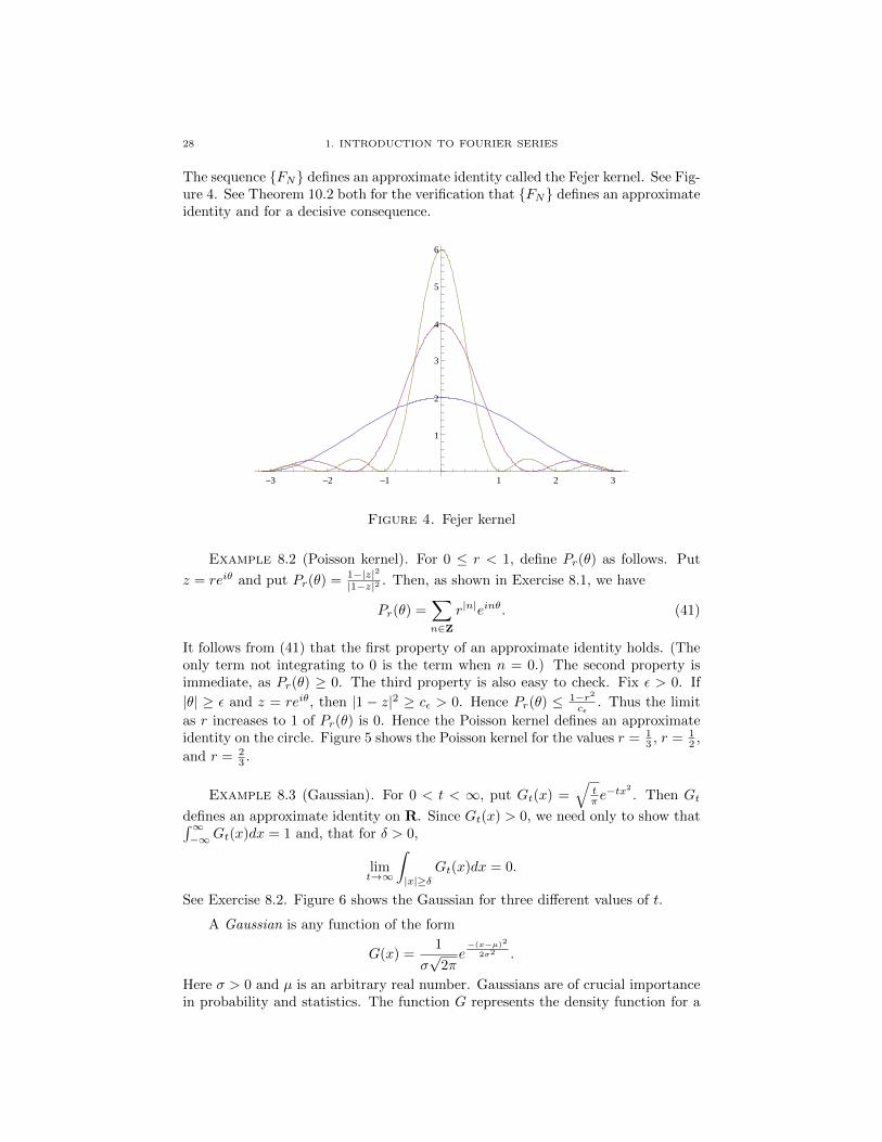
The sequence FN defines an approximate identity called the Fejer kernel. See Fig-ure 4. See Theorem 10.2 both for the verification that FN defines an approximateidentity and for a decisive consequence.
-3 -2 -1 1 2 3
1
2
3
4
5
6
Figure 4. Fejer kernel
Example 8.2 (Poisson kernel). For 0 ≤ r < 1, define Pr(θ) as follows. Put
z = reiθ and put Pr(θ) = 1−|z|2|1−z|2 . Then, as shown in Exercise 8.1, we have
Pr(θ) =∑n∈Z
r|n|einθ. (41)
It follows from (41) that the first property of an approximate identity holds. (Theonly term not integrating to 0 is the term when n = 0.) The second property isimmediate, as Pr(θ) ≥ 0. The third property is also easy to check. Fix ε > 0. If
|θ| ≥ ε and z = reiθ, then |1 − z|2 ≥ cε > 0. Hence Pr(θ) ≤ 1−r2cε
. Thus the limit
as r increases to 1 of Pr(θ) is 0. Hence the Poisson kernel defines an approximateidentity on the circle. Figure 5 shows the Poisson kernel for the values r = 1
3 , r = 12 ,
and r = 23 .
Example 8.3 (Gaussian). For 0 < t < ∞, put Gt(x) =√
tπ e−tx2
. Then Gt
defines an approximate identity on R. Since Gt(x) > 0, we need only to show that∫∞−∞Gt(x)dx = 1 and, that for δ > 0,
limt→∞
∫|x|≥δ
Gt(x)dx = 0.
See Exercise 8.2. Figure 6 shows the Gaussian for three different values of t.
A Gaussian is any function of the form
G(x) =1
σ√
2πe−(x−µ)2
2σ2 .
Here σ > 0 and µ is an arbitrary real number. Gaussians are of crucial importancein probability and statistics. The function G represents the density function for a

9. DEFINITION OF FOURIER SERIES 29
-3 -2 -1 1 2 3Θ
1
2
3
4
5
Pr HΘL
Figure 5. Poisson kernel
normal probability distribution with mean µ and variance σ2. In Example 8.3, weare setting µ = 0 and σ2 = 1
2t . When we let t tend to infinity, we are making thevariance tend to zero and clustering the probability around the mean, thus givingan intuitive understanding of why Gt is an approximate identity. By contrast, whenwe let t tend to 0, the variance tends to infinity and the probability distributionspreads out. We will revisit this situation in Chapter 3.
-6 -4 -2 2 4 6
0.1
0.2
0.3
0.4
Figure 6. Gaussian kernel
Exercise 8.1. Verify (41). (Hint: Sum two geometric series.)
Exercise 8.2. Verify the statements in Example 8.3.
9. Definition of Fourier series
An infinite series of the form∑n=∞n=−∞ cne
inθ is called a trigonometric series.Such a series need not converge.
30 1. INTRODUCTION TO FOURIER SERIES
Let f be an integrable function on the circle. For n ∈ Z we define its Fouriercoefficients by
f(n) =1
2π
∫ 2π
0
f(x)e−inxdx.
Note by (9) that the coefficient cj of a trig polynomial f is precisely the Fourier
coefficient f(j). Sometimes we write F(f)(n) = f(n). One reason is that thisnotation helps us think of F as an operator on functions. If f is integrable onthe circle, then F(f) is a function on the integers, called the Fourier transform off . Later we will consider Fourier transforms for functions defined on the real line.Another reason for the notation is that typographical considerations suggest it.
Definition 9.1. The Fourier series of an integrable function f on the circle isthe trigonometric series ∑
n∈Z
f(n)einx.
When considering convergence of a trigonometric series, we generally considerlimits of the symmetric partial sums defined by
SN (x) =
N∑n=−N
aneinx.
Considering the parts for n positive and n negative separately makes things morecomplicated. See [SS].
The Fourier series of an integrable function need not converge. Much of thesubject of Fourier analysis arose from asking various questions about convergence.For example, under what conditions does the Fourier series of f converge pointwiseto f , or when is the series summable to f using some more complicated summabilitymethod. We discuss some of these summability methods in the next section.
Lemma 9.1 (properties of Fourier coefficients). The following Fourier transformformulas hold:
(1) F(f + g) = F(f) + F(g)(2) F(cf) = cF(f)
(3) For all n, F(f)(n) = f(n) = f(−n) = F(f)(−n).(4) For all n, |F(f)(n)| ≤ ||f ||L1 . Equivalently, ||F(f)||L∞ ≤ ||f ||L1 .
Proof. See Exercise 9.1.
The first two properties express the linearity of the integral. The third propertygeneralizes the palindrome property of real trig polynomials. We will use the fourthproperty many times in the sequel.
We also note the relationship between anti-derivatives and Fourier coefficients.
Lemma 9.2. Let f be Riemann integrable (hence bounded). Assume that f(0) =1
2π
∫f(u)du = 0. Put F (x) =
∫ x0f(u)du. Then F is continuous and for n 6= 0,
F (n) =f(n)
in. (42)
9. DEFINITION OF FOURIER SERIES 31
Proof. The following inequality implies the continuity of F :
|F (x)− F (y)| =∣∣∣∣∫ x
y
f(u)du
∣∣∣∣ ≤ |x− y| ||f ||L∞ .Formula (42) follows either by integration by parts (see Exercise 9.1) or by inter-changing the order of integration:
F (n) =1
2π
∫ 2π
0
(∫ x
0
f(u)du
)e−inxdx =
1
2π
∫ 2π
0
(∫ 2π
u
e−inxdx
)f(u)du
=1
2π
∫ 2π
0
1
−in(1− e−inu)f(u)du =
f(n)
in,
since∫f(u)du = 0.
See Exercise 9.4 for a generalization of this Lemma. The more times f isdifferentiable, the faster the Fourier coefficients must decay at infinity.
Exercise 9.1. Prove Lemma 9.1. Prove Lemma 9.2 using integration by parts.
Exercise 9.2. Find the Fourier series for cos2N (θ). (Hint: Don’t do anyintegrals!)
Exercise 9.3. Assume f is real-valued. Under what additional condition canwe conclude that its Fourier coefficients are real? Under what condition are thecoefficients purely imaginary?
Exercise 9.4. Assume that f is k times continuously differentiable. Show thatthere is a constant C such that ∣∣∣f(n)
∣∣∣ ≤ C
nk.
Exercise 9.5. Assume that f(x) = −1 for −π < x < 0 and f(x) = 1 for0 < x < π. Compute the Fourier series for f .
Exercise 9.6. Put f(x) = eax for 0 < x < 2π. Compute the Fourier series forf .
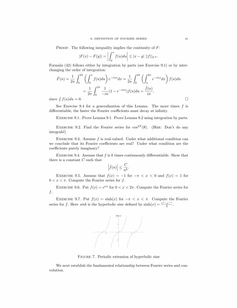
Exercise 9.7. Put f(x) = sinh(x) for −π < x < π. Compute the Fourier
series for f . Here sinh is the hyperbolic sine defined by sinh(x) = ex−e−x2 .
-5 5
-5
5
Sinh HxL
Figure 7. Periodic extension of hyperbolic sine
We next establish the fundamental relationship between Fourier series and con-volution.

32 1. INTRODUCTION TO FOURIER SERIES
Theorem 9.1. If f and g are integrable, then f ∗g is continuous and F(f ∗g) =F(f)F(g). In other words, for all n we have
F(f ∗ g)(n) = (f ∗ g) (n) = f(n)g(n) = F(f)(n)F(g)(n). (43)
Proof. The proof is computational when f and g are continuous. We computethe left-hand side of (43) as a double integral, and then interchange the order ofintegration. The general case then follows using the approximation Lemma 7.1.
Here are the details. Suppose first that f and g are continuous. Then
F(f ∗ g)(n) =1
2π
∫ 2π
0
(1
2π
∫ 2π
0
f(y)g(x− y)dy
)e−inxdx.
By continuity, we may interchange the order of integration, obtaining
F(f ∗ g)(n) = (1
2π)2
∫ 2π
0
f(y)
(∫ 2π
0
g(x− y)e−inxdx
)dy.
Change variables by putting x − y = t. Then use e−in(y+t) = e−inye−int, and theresult follows.
Next, assume f and g are Riemann integrable, hence bounded. By Lemma7.1 we can find sequences of continuous functions fk and gk such that ||fk||L∞ ≤||f ||L∞ , also ||f − fk||L1 → 0, and similarly for gk. By the usual adding andsubtracting trick,
f ∗ g − fk ∗ gk = ((f − fk) ∗ g) + (fk ∗ (g − gk)) . (44)
Since g and each fk is bounded, both terms on the right-hand side of (44) tend to0 uniformly. Therefore fk ∗ gk tends to f ∗ g uniformly. Since the uniform limit ofcontinuous functions is continuous, f ∗ g is itself continuous. Since fk tends to f inL1 and (by property (4) from Lemma 9.1)
|fk(n)− f(n)| ≤ 1
2π
∫ 2π
0
|fk − f |, (45)
it follows that |fk(n) − f(n)| converges to 0 for all n. Similarly |gk(n) − g(n)|converges to 0 for all n. Hence, for each n, fk(n)gk(n) converges to f(n)g(n). Since(43) holds for fk and gk, it holds for f and g.
By the previous result, the function f ∗ g is continuous when f and g areassumed only to be integrable. Convolutions are often used to regularize a function.For example, if f is integrable and g is infinitely differentiable, then f ∗g is infinitelydifferentiable. In Chapter 3 we will use this idea when gn defines an approximateidentity consisting of smooth functions.
10. Summability methods
We introduce two notions of summability, Cesaro summability and Abel summa-bility, which arise in studying the convergence of Fourier series.
First we make an elementary remark. Let An be a sequence of complexnumbers. Let σN denote the average of the first N terms:
σN =A1 +A2 + ...+AN
N.

10. SUMMABILITY METHODS 33
If AN → L, then σN → L as well. We will prove this fact below. It appliesin particular when AN is the N -th partial sum of a sequence an. There existexamples where AN does not converge but σN does converge. See Theorem 10.1.We therefore obtain a more general notion of summation for the infinite series
∑an.
Suppose next that∑an converges to L. For 0 ≤ r < 1, put f(r) =
∑anr
n.We show below that limr→1 f(r) = L. (Here we are taking the limit as r increasesto 1.) There exist series
∑an such that
∑an diverges but this limit of f(r) exists.
A simple example is given by an = (−1)n+1. A more interesting example is givenby an = n(−1)n+1.
Definition 10.1. Let an be a sequence of complex numbers. Let AN =∑Nj=1 aj . Let σN = 1
N
∑Nj=1Aj . For 0 ≤ r < 1 we put FN (r) =
∑Nj=1 ajr
j .
(1)∑∞
1 aj converges to L if limN→∞AN = L.(2)
∑∞1 aj is Cesaro summable to L if limN→∞ σN = L.
(3)∑∞
1 aj is Abel summable to L if limr→1 limN→∞ FN (r) = L.
Theorem 10.1. Let an be a sequence of complex numbers.
(1) If∑an converges to L, then
∑an is Cesaro summable to L. The converse
fails.(2) If
∑an is Cesaro summable to L, then
∑an is Abel summable to L. The
converse fails.
Proof. We start by showing that the converse assertions are false. First putan = (−1)n+1. The series
∑an certainly diverges, because the terms do not tend
to 0. On the other hand, the partial sum AN equals 0 if N is even and equals 1 ifN is odd. Hence σ2N = 1
2 and σ2N+1 = N+12N+1 →
12 . Thus limN→∞ σN = 1
2 . Thus∑an is Cesaro summable but not convergent.
Next put an = n(−1)n+1. Computation shows that A2N = −N and A2N+1 =N + 1. It follows that σ2N = 0 and that σ2N+1 = N+1
2N+1 . These expressions have
different limits and hence limN σN does not exist. On the other hand, for |r| < 1,
∞∑n=1
n(−1)n+1rn = r
∞∑1
n(−r)n−1 =r
(1 + r)2.
Letting r tend upwards to 1 gives the limiting value of 14 . Hence
∑an is Abel
summable to 14 but not Cesaro summable.
1) Suppose that∑an = L. Replace a1 with a1 − L and keep all the other
terms the same. The new series sums to 0. Furthermore, each partial sum ANis decreased by L. Hence the Cesaro means σN get decreased by L as well. Ittherefore suffices to consider the case where
∑an = 0. Fix ε > 0. Since AN tends
to 0, we can find an N0 such that N ≥ N0 implies |AN | < ε2 .
We have for N ≥ N0,
σN =1
N
N0−1∑j=1
Aj +1
N
N∑j=N0
Aj . (46)
Since N0 is fixed, the first term tends to 0 as N tends to infinity, and hence itsabsolute value is bounded by ε
2 for large enough N . The absolute value of the
second term is bounded by ε2N−N0+1
N and hence by ε2 because N ≥ N0 ≥ 1. The
conclusion follows.
34 1. INTRODUCTION TO FOURIER SERIES
2) This proof is a bit elaborate and uses summation by parts. Suppose firstthat σN → 0. For 0 ≤ r < 1 we claim that
(1− r)2∞∑n=1
nσnrn =
∞∑n=1
anrn. (47)
We wish to show that the limit as r tends to 1 of the right-hand side of (47) existsand equals 0. Given the claim, consider ε > 0. We can find N0 such that n ≥ N0
implies |σn| < ε2 . We break up the sum on the left-hand side of (47) into terms
where n ≤ N0 − 1 and the rest. The absolute value of the first part is a finite sumtimes (1− r)2 and hence can be made at most ε
2 by choosing r close enough to 1.
Note that∑∞n=1 nr
n−1 = 1(1−r)2 . The second term T can then be estimated by
|T | ≤ (1− r)2 ε
2
∞∑N0
nrn ≤ (1− r)2 ε
2
∞∑1
nrn = rε
2.
Hence, given the claim, by choosing r close enough to 1 we can make the absolutevalue of (47) as small as we wish. Thus
∑an is Abel summable to 0. As above,
the case where σN tends to L reduces to the case where it tends to 0.It remains to prove (47), which involves summation by parts twice.
N∑1
anrn = ANr
N −N−1∑
1
An(rn+1 − rn) = ANrN + (1− r)
N−1∑1
Anrn.
Next we use summation by parts on∑N−1
1 Anrn:
N−1∑1
Anrn = (N − 1)σN−1r
N−1 −N−2∑
1
nσn(rn+1 − rn)
= (N − 1)σN−1rN−1 + (1− r)
N−2∑1
nσnrn.
Note that AN = NσN − (N − 1)σN−1. Hence we obtain
N∑1
anrn =
(NσN − (N − 1)σN−1)rN + (1− r)rN−1(N − 1)σN−1 + (1− r)2N−2∑
1
nσnrn. (48)
Since |r| < 1, lim(NrN ) = 0. Since also σN is bounded, each of the terms in (48)
other than the sum converges to 0. Thus∑N
1 anrn converges to (1−r)2
∑∞1 nσnr
n,as desired.
The reader should note the similarities in the proofs of Theorem 8.1 and The-orem 10.1. The same ideas appear also in one of the standard proofs of the Funda-mental Theorem of Calculus.
Cesaro summability will be important in our analysis of the series∑∞n=1
sin(nx)n .
We will prove a general result about convergence to f(x) of the Cesaro means ofthe Fourier series of the integrable function f at points x where f is continuous.

10. SUMMABILITY METHODS 35
Then we will compute the Fourier series for the function x on the interval [0, 2π].It then follows for 0 < x < 2π that
∞∑n=1
sin(nx)
n=π − x
2.
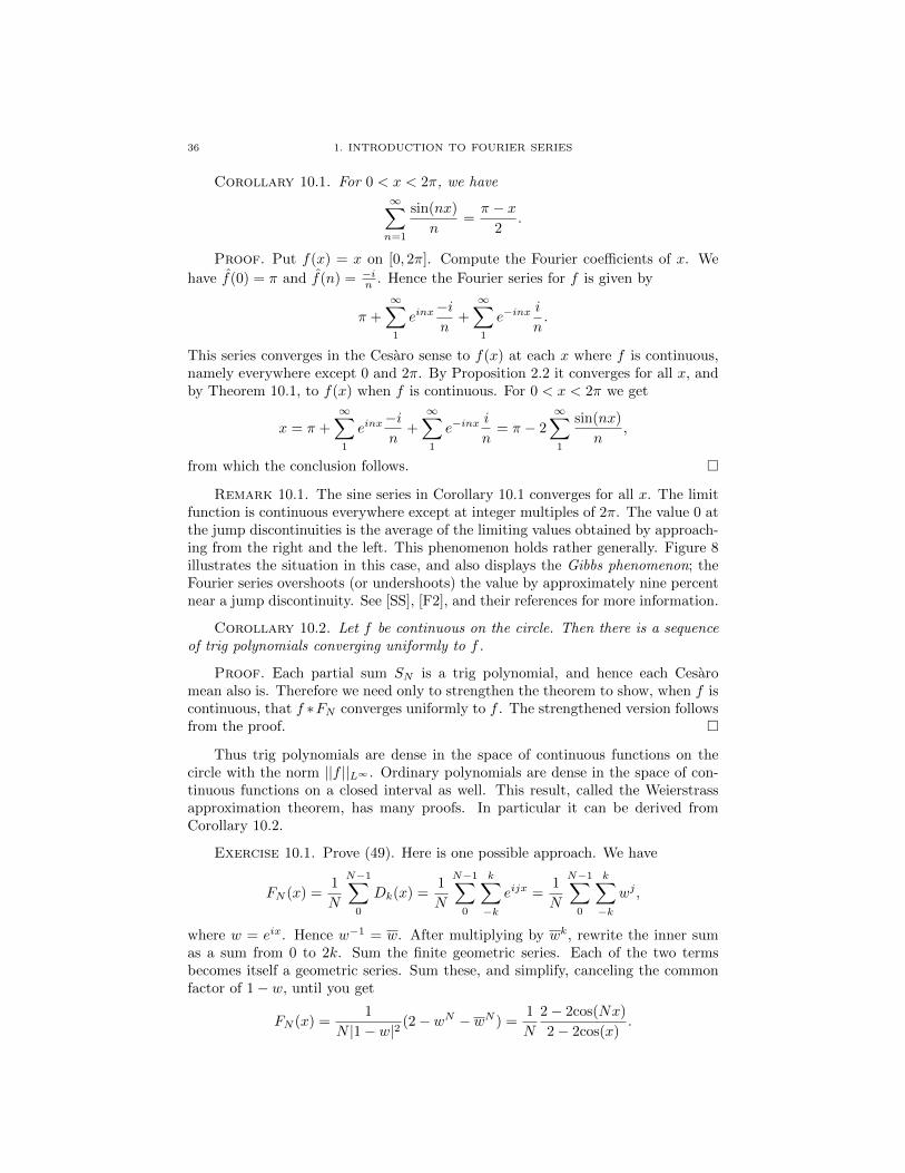
Note that equality fails at 0 and 2π. Figure 8 shows two partial sums of the series.
-6 -4 -2 2 4 6
-1.5
-1.0
-0.5
0.5
1.0
1.5
Figure 8. Approximations to the sawtooth function
Recall that SN (x) =∑N−N f(N)einx denotes the symmetric partial sums of the
Fourier series of f .
Theorem 10.2. Suppose f is integrable on [−π, π] and f is continuous at x.The Fourier series for f at x is Cesaro summable to f(x).
Proof. Put DK(x) =∑K−K e
inx. Define FN by
FN (x) =D0(x) +D1(x) + ...+DN−1(x)
N.
Note that σN (f)(x) = (f ∗ FN )(x). We claim that FN defines an approximateidentity.
Since each DK integrates to 1, each FN integrates to 1. The first property ofan approximate identity therefore holds. A computation (Exercise 10.1) shows that
FN (x) =1
N
sin2(Nx2 )
sin2(x2 ). (49)
Since FN ≥ 0, the second property of an approximate identity is automatic. Thethird is easy to prove. It suffices to show for each ε with 0 < ε < π that
limN→∞
∫ π
ε
FN (x)dx = 0.
But, for x in the interval [ε, π], the term 1sin2( x2 )
is bounded above by a constant and
the term sin2(Nx2 ) is bounded above by 1. Hence FN ≤ cN and the claim follows.
The conclusion of the Theorem now follows by Theorem 8.1.
36 1. INTRODUCTION TO FOURIER SERIES
Corollary 10.1. For 0 < x < 2π, we have∞∑n=1
sin(nx)
n=π − x
2.
Proof. Put f(x) = x on [0, 2π]. Compute the Fourier coefficients of x. We
have f(0) = π and f(n) = −in . Hence the Fourier series for f is given by
π +
∞∑1
einx−in
+
∞∑1
e−inxi
n.
This series converges in the Cesaro sense to f(x) at each x where f is continuous,namely everywhere except 0 and 2π. By Proposition 2.2 it converges for all x, andby Theorem 10.1, to f(x) when f is continuous. For 0 < x < 2π we get
x = π +∞∑1
einx−in
+∞∑1
e−inxi
n= π − 2
∞∑1
sin(nx)
n,
from which the conclusion follows.
Remark 10.1. The sine series in Corollary 10.1 converges for all x. The limitfunction is continuous everywhere except at integer multiples of 2π. The value 0 atthe jump discontinuities is the average of the limiting values obtained by approach-ing from the right and the left. This phenomenon holds rather generally. Figure 8illustrates the situation in this case, and also displays the Gibbs phenomenon; theFourier series overshoots (or undershoots) the value by approximately nine percentnear a jump discontinuity. See [SS], [F2], and their references for more information.
Corollary 10.2. Let f be continuous on the circle. Then there is a sequenceof trig polynomials converging uniformly to f .
Proof. Each partial sum SN is a trig polynomial, and hence each Cesaromean also is. Therefore we need only to strengthen the theorem to show, when f iscontinuous, that f ∗FN converges uniformly to f . The strengthened version followsfrom the proof.
Thus trig polynomials are dense in the space of continuous functions on thecircle with the norm ||f ||L∞ . Ordinary polynomials are dense in the space of con-tinuous functions on a closed interval as well. This result, called the Weierstrassapproximation theorem, has many proofs. In particular it can be derived fromCorollary 10.2.
Exercise 10.1. Prove (49). Here is one possible approach. We have
FN (x) =1
N
N−1∑0
Dk(x) =1
N
N−1∑0
k∑−k
eijx =1
N
N−1∑0
k∑−k
wj ,
where w = eix. Hence w−1 = w. After multiplying by wk, rewrite the inner sumas a sum from 0 to 2k. Sum the finite geometric series. Each of the two termsbecomes itself a geometric series. Sum these, and simplify, canceling the commonfactor of 1− w, until you get
FN (x) =1
N |1− w|2(2− wN − wN ) =
1
N
2− 2cos(Nx)
2− 2cos(x).

11. THE LAPLACE EQUATION 37
We finally obtain (49) after using the identity
sin2(α
2) =
1− cos(α)
2.
Exercise 10.2. Verify the previous trig identity using complex exponentials.
Exercise 10.3. Put f(x) = 1log(x) . Show that f is convex and decreasing.
Conclude that f(x+ 2) + f(x) ≥ 2f(x+ 1).
Exercise 10.4. Find the following limit:
limx→∞
x
(1
log(x+ 2)+
1
log(x)− 2
log(x+ 1)
).
Exercise 10.5. Use (49) and Exercise 10.3 to solve Exercise 2.6. (Again sumby parts twice.) Exercise 2.3 might also be useful.
Remark 10.2. In solving Exercise 10.5, one must include the first term.
Exercise 10.6. Derive the Weierstrass approximation theorem from Corollary10.2. Suggestion. First show that the Taylor polynomials of eix uniformly approx-imate it on any closed and bounded interval. Thus any trig polynomial can beuniformly approximated by ordinary polynomials.
Exercise 10.7. If sn is a monotone sequence of real numbers, show that
the averages σN = 1N
∑Nj=1 sj also define a monotone sequence. Give an example
where the converse assertion is false.
11. The Laplace equation
In this section we connect ideas from Abel summability to the Dirichlet problemfor the Laplace equation.
We have defined Abel summability of a series∑∞n=0 zn of complex numbers.
For Fourier series, we make a small change and consider Abel summability of theseries
∑∞−∞ ane
inθ. Thus we consider∑n∈Z
anr|n|einθ, (50)
and we let r increase to 1. The series in (50) turns out to have a simple expression;it is the convolution of the Fourier series with the Poisson kernel. Since the Poissonkernel is an approximate identity, our next result will follow easily.
Theorem 11.1. Suppose h is integrable on the circle. Then the Fourier seriesof h is Abel summable to h at each point of continuity of h. If h is continuous onthe circle, then the Abel means of its Fourier series converge uniformly to h.
Proof. Recall that Pr(θ) = 1−|z|2|1−z|2 when z = reiθ. We have noted that Pr is
an approximate identity and that
Pr(θ) =∑n∈Z
r|n|einθ.
The Abel means of the Fourier series for h are then∑n∈Z
h(n)r|n|einθ = (Pr ∗ h)(θ).

38 1. INTRODUCTION TO FOURIER SERIES
By Theorem 8.1 the Abel means converge to h(θ) at each point where h is contin-uous. Also by Theorem 8.1, the convergence is uniform if h is continuous.
We recall that a twice differentiable function u of two real variables is calledharmonic if ∆(u) = 0; that is,
∆(u) = uxx + uyy = 0.
The Dirichlet problem is perhaps the most fundamental boundary-value prob-lem in applied mathematics. We are given a continuous function h on the boundaryof an open set Ω, and we wish to find a harmonic function u on Ω such that u = hon the boundary.
For us, Ω will be the unit disk in C; its boundary is the unit circle. Suppose his given by a Fourier series,
h(θ) =∑n∈Z
aneinθ.
Then the solution u to the Dirichlet problem is uniquely determined and satisfies
u(z) = u(reiθ) =∑n∈Z
r|n|aneinθ. (51)
Before proving this result (Theorem 11.3), we recall one of the basic ideas fromcomplex variable theory, the notion of radius of convergence of a power series.
Theorem 11.2. Given a power series∑∞n=1 anz
n, there is a non-negative realnumber R, or the value infinity, such that the series converges for |z| < R anddiverges for |z| > R. The number R can be computed by Hadamard’s formula
R = supr : |an|rn is a bounded sequence. (52)
If R = 0, then the series converges only if z = 0. If 0 ≤ r < R, the the seriesconverges absolutely and uniformly for |z| ≤ r.
Proof. Define R by (52). If |z| > R, then the terms of the series are un-bounded, and hence the series diverges. Next assume that 0 ≤ ρ < r < R. Assumethat |an|rn ≤ M . We claim that
∑anz
n converges absolutely and uniformly in|z| ≤ ρ. The claim follows by the comparison test and the convergence of ageometric series with ratio t = ρ
r :∑|anzn| ≤
∑|an|ρn =
∑|an|rn(
ρ
r)n ≤M
∑tn.
Each assertion follows.
Remark 11.1. We also can compute R by the root test. See Exercise 11.4.
The Laplacian ∆ has a convenient expression using complex partial derivatives:
∆(u) = 4uzz = 4∂2u
∂z∂z.
Here the complex partial derivatives are defined by
∂
∂z=
1
2(∂
∂x− i ∂
∂y)
∂
∂z=
1
2(∂
∂x+ i
∂
∂y).
Exercise 11.1. Verify the formula ∆(u) = 4uzz.

11. THE LAPLACE EQUATION 39
Exercise 11.2. Show that the Laplacian in polar coordinates is given as fol-lows:
∆(u) = urr +1
rur +
1
r2uθθ.
Exercise 11.3. Use the previous exercise to show that the real and imaginaryparts of zn are harmonic for n a positive integer.
Exercise 11.4. Given the series∑anz
n, put L = lim sup(|an|1n ). Show that
the radius of convergence R satisfies R = 1L .
Exercise 11.5. Give three examples of power series with radius of convergence1 with the following true. The first series converges at no points of the unit circle,the second series converges at some but not all points of the unit circle, and thethird series converges at all points of the unit circle.
Exercise 11.6. Let p be a polynomial. Show that the series∑
(−1)np(n) isAbel summable. More generally, show that
∑∞0 p(n)zn is a polynomial in 1
1−zwith no constant term. Hence the limit, as we approach the unit circle from within,exists at every point except 1.
By analogy with the wave equation, the formula for the Laplacian in complexnotation suggests that a function u = u(x, y) is harmonic if and only if it can bewritten u(x, y) = f(z) + g(z), for functions f and g of the indicated one complexvariable. In particular it suggests that a real-valued function is harmonic if andonly if it is the real part of a complex analytic function.
We use these considerations to revisit the Dirichlet problem. Let h be contin-uous on the circle.
Theorem 11.3. Suppose h is continuous on the unit circle. Put
u(reiθ) = (Pr ∗ h)(θ).
Then u is infinitely differentiable on the unit disk, u is harmonic, and u = h on thecircle.
Proof. Since h is continuous, the Fourier coefficients h(n) are bounded. Hencefor each r < 1 the series in (51) converges absolutely. Put z = reiθ and writeu(reiθ) = (Pr ∗ h)(θ). We have
u(reiθ) =
∞∑n=0
h(n)rneinθ +
∞∑n=1
h(−n)rne−inθ =
∞∑n=0
h(n)zn +
∞∑n=1
h(−n)zn
= f(z) + g(z).
Each zn or zn is harmonic. The power series for f and g each converge absolutelyand uniformly in the unit disk. Hence they represent infinitely differentiable func-tions. We can therefore differentiate term by term to conclude that u is harmonic.Since h is continuous, h(θ) = limr→1 u(reiθ).
The Dirichlet problem for domains (open and connected sets) more general thanthe unit disk is of fundamental importance in applied mathematics. Amazinglyenough, the solution for the unit disk extends to much more general situations.By the Riemann mapping theorem, each simply connected domain other than Cis conformally equivalent to the unit disk. Hence one can transfer the problem to

40 1. INTRODUCTION TO FOURIER SERIES
the disk and solve it there. See [A] or [D2] for additional discussion. Exercise 11.9provides an important formula.
We make some additional remarks about the Cauchy-Riemann equations. Sup-pose f is complex analytic in an open set, and we write f = u + iv there. Thenu and v are harmonic and satisfy the system of PDE ux = vy and uy = −vx.These two equations are equivalent to the simpler statement fz = 0 (which yields
fz = 0 as well). Since u = f+f2 (and v has a similar formula), it follows from the
formula ∆ = 4 ∂2
∂z∂z that u and v are harmonic. Furthermore, the Cauchy-Riemannequations guarantee that the level curves of u and v intersect orthogonally. Thisgeometric fact partially explains why complex analytic functions are useful in ap-plied subjects such as fluid flow.
The next exercise approaches the Laplace equation by way of polar coordinatesand separation of variables. It presages spherical harmonics, discussed in Section13 of Chapter 2, where the circle gets replaced with the sphere.
Exercise 11.7. Use Exercise 11.2 and separation of variables to find solutionsof the Laplace equation ∆(f) = 0. Your answers should be in the form rneinθ.Compare with Exercise 11.3.
Exercise 11.8. Graph some level sets of the real and imaginary parts of f ,when f(z) = z2, when f(z) = ez, and when f(z) = log(z), for some branch of thelogarithm.
Exercise 11.9. Assume that f is complex analytic and that h is twice dif-ferentiable in a neighborhood of the image of f . Compute the Laplacian of h f .Suggestion: Use the formula from Exercise 11.1.
Exercise 11.10. Discuss the validity of the formula
log(x+ iy) =1
2log(x2 + y2) + i tan−1(
y
x).
Exercise 11.11. Assume 0 ≤ r < 1. Find formulas for∞∑n=1
rncos(nθ)
nand
∞∑n=1
rnsin(nθ)
n.
Suggestion: Start with the geometric series∞∑n=0
zn =1
1− z,
valid for |z| < 1. Integrate to obtain a series for −log(1− z). Replace z with reiθ,equate real and imaginary parts of the result, and use Exercise 11.10.
Fourier’s original work considered the heat equation ut = ∆(u). The Laplaceequation can be regarded as the steady-state solution of the heat equation.
We pause to consider the heat equation by way of separation of variables. Putu(x, y, t) = A(x, y)B(t). The heat equation becomes ∆A(x, y)B(t) = A(x, y)B′(t),
and hence ∆AA = B′
B = λ for some constant λ, and B(t) = eλt. To guarantee that Btends to zero at∞, the constant λ must be negative. We also obtain the eigenvalueproblem ∆A = λA. We then introduce polar coordinates and use the formula inExercise 11.2. Doing so leads to the equation
r2Arr + rAr +Aθθ = λr2A.
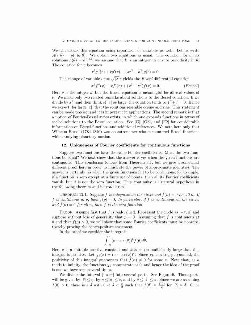
12. UNIQUENESS OF FOURIER COEFFICIENTS FOR CONTINUOUS FUNCTIONS 41
We can attack this equation using separation of variables as well. Let us writeA(r, θ) = g(r)h(θ). We obtain two equations as usual. The equation for h hassolutions h(θ) = e±ikθ; we assume that k is an integer to ensure periodicity in θ.The equation for g becomes
r2g′′(r) + rg′(r)− (λr2 − k2)g(r) = 0.
The change of variables x =√|λ|r yields the Bessel differential equation
x2f ′′(x) + xf ′(x) + (x2 − ν2)f(x) = 0. (Bessel)
Here ν is the integer k, but the Bessel equation is meaningful for all real values ofν. We make only two related remarks about solutions to the Bessel equation. If wedivide by x2, and then think of |x| as large, the equation tends to f ′′+f = 0. Hencewe expect, for large |x|, that the solutions resemble cosine and sine. This statementcan be made precise, and it is important in applications. The second remark is thata notion of Fourier-Bessel series exists, in which one expands functions in terms ofscaled solutions to the Bessel equation. See [G], [GS], and [F2] for considerableinformation on Bessel functions and additional references. We note here only thatWilhelm Bessel (1784-1846) was an astronomer who encountered Bessel functionswhile studying planetary motion.
12. Uniqueness of Fourier coefficients for continuous functions
Suppose two functions have the same Fourier coefficients. Must the two func-tions be equal? We next show that the answer is yes when the given functions arecontinuous. This conclusion follows from Theorem 8.1, but we give a somewhatdifferent proof here in order to illustrate the power of approximate identities. Theanswer is certainly no when the given functions fail to be continuous; for example,if a function is zero except at a finite set of points, then all its Fourier coefficientsvanish, but it is not the zero function. Thus continuity is a natural hypothesis inthe following theorem and its corollaries.
Theorem 12.1. Suppose f is integrable on the circle and f(n) = 0 for all n. Iff is continuous at p, then f(p) = 0. In particular, if f is continuous on the circle,
and f(n) = 0 for all n, then f is the zero function.
Proof. Assume first that f is real-valued. Represent the circle as [−π, π] andsuppose without loss of generality that p = 0. Assuming that f is continuous at0 and that f(p) > 0, we will show that some Fourier coefficients must be nonzero,thereby proving the contrapositive statement.
In the proof we consider the integrals∫ π
−π(c+ cos(θ))kf(θ)dθ.
Here c is a suitable positive constant and k is chosen sufficiently large that thisintegral is positive. Let χk(x) = (c + cos(x))k. Since χk is a trig polynomial, the
positivity of this integral guarantees that f(n) 6= 0 for some n. Note that, as ktends to infinity, the functions χk concentrate at 0, and hence the idea of the proofis one we have seen several times.
We divide the interval [−π, π] into several parts. See Figure 9. These partswill be given by |θ| ≤ η, by η ≤ |θ| ≤ δ, and by δ ≤ |θ| ≤ π. Since we are assuming
f(0) > 0, there is a δ with 0 < δ < π2 such that f(θ) ≥ f(0)
2 for |θ| ≤ δ. Once

42 1. INTRODUCTION TO FOURIER SERIES
δ is chosen, we find a small positive c such that cos(θ) ≤ 1 − 3c2 when |θ| ≥ δ.
Doing so is possible because cos(θ) is bounded away from 1 there. The inequality|c+ cos(θ)| ≤ 1− c
2 for |θ| ≥ δ follows.We want χk(θ) big near 0. We next find η with 0 < η < δ such that c+cos(θ) ≥
c2 + 1 for |θ| ≤ η. Doing so is possible because 1− cos(θ) is small near 0.
On the part where θ is close to 0,∫χkf ≥ C(1 + ( c2 ))k. On the part where
η ≤ |θ| ≤ δ,∫χkf ≥ 0. On the part where |θ| ≥ δ,∣∣∣∣∫ χk f
∣∣∣∣ ≤ C(1− c
2)k. (53)
We gather this information. The integral∫|θ|≤η
χk(x)f(x)dx
actually tends to infinity with k. The integral over the set where η ≤ |θ| ≤ δ yieldsa positive number. By (53), the integral over the remaining part is bounded as ktends to infinity. Thus the sum of the three pieces tends to infinity and hence∫ π
−πχk(x)f(x)dx > 0
for large k. Hence some Fourier coefficient of f must be nonzero.The case when f is complex-valued follows by applying the above reasoning to
its real and imaginary parts. Note that the real part of f is f+f2 and the imaginary
part of f is f−f2i . By Lemma 9.1 we know that
f(n) = f(−n).
Hence all the Fourier coefficients of f vanish if and only if all the Fourier coefficientsof its real and imaginary parts vanish.
Corollary 12.1. If both f and g are continuous on the circle, and f(n) = g(n)for all n, then f = g.
Proof. The function f−g is continuous and all its Fourier coefficients vanish.Hence f − g = 0 and thus f = g.
Corollary 12.2. Suppose∑|f(n)| converges and f is continuous. Then SN
converges uniformly to f .
Proof. Recall that SN (f)(x) =∑N−N e
inxf(n). Each SN (f) is continuous,and the hypothesis guarantees that SN (f) converges uniformly. Hence it has acontinuous limit g. But g and f have the same Fourier coefficients. By Corollary12.1, f = g.
Assuming the continuity of f is not adequate to ensure that the Fourier seriesof f converges absolutely. If f is twice differentiable, however, then a simple com-
putation shows that |f(n)| ≤ Cn2 and hence the Fourier series for f does converge
absolutely, as∑
1n2 converges. Since
∑1np converges for p > 1, we see that an
inequality of the form
|f(n)| ≤ C
np(54)

13. INEQUALITIES 43
-Π -∆ -Η Η ∆ Π
f H0L
2
f H0L
Figure 9. Proof of Theorem 12.1
for p > 1 also guarantees absolute convergence. In Chapter 2 we prove a relatedbut more difficult result involving Holder continuous functions.
Remark 12.1. There exist continuous functions whose Fourier series do notconverge at all points. Constructing such a function is a bit difficult. See [K] orpages 83-87 in [SS].
13. Inequalities
In this section we use Fourier series to establish inequalities. The first exampleis a famous inequality of Hilbert. Rather than proving it directly, we derive it froma general result. There is a vast literature on generalizations of Hilbert’s inequality.See [HLP], [B], [S] and their references.
Theorem 13.1 (Hilbert’s inequality). Let zn (for n ≥ 0) be a sequence ofcomplex numbers with
∑|zn|2 finite. Then
|∞∑
j,k=0
zjzk1 + j + k
| ≤ π∞∑k=0
|zk|2. (55)
Furthermore the constant π is the smallest possible.
Hilbert’s inequality follows by choosing g(t) = i(π − t)e−it in Theorem 13.2below. With this choice of g we have g(n) = 1
n+1 and hence the j, k entry of the
infinite matrix C is 11+j+k . Furthermore |g| is bounded by π.
The inequality can be stated in equivalent ways. For example, by choosingg(t) = i(π − t) we have g(n) = 1
n and we obtain the following:
|∞∑
j,k=1
zjzkj + k
| ≤ π∞∑k=1
|zk|2.
Polarization yields, in case both sequences zk and wk are square-summable,
|∞∑
j,k=1
zjwkj + k
| ≤ π
( ∞∑k=1
|zk|2) 1
2( ∞∑k=1
|wk|2) 1
2
. (56)
We omit the proof that π is the smallest possible constant. [HLP] has severalproofs. We do remark however that equality holds in (55) only if z is the zero

44 1. INTRODUCTION TO FOURIER SERIES
sequence. In other words, unless z is the zero sequence, one can replace ≤ with <in (55).
We can also write (55) or (56) in terms of integrals rather than sums:∫ ∞0
∫ ∞0
f(x)g(y)
x+ ydxdy ≤ π||f ||L2 ||g||L2 , (57.1)
where the L2 norm is taken over [0,∞). See Exercise 13.3. This formulationsuggests a generalization due to Hardy. Let 1
p + 1q = 1. Then p, q are called
conjugate exponents. Hardy’s result gives the following inequality:∫ ∞0
∫ ∞0
f(x)g(y)
x+ ydxdy ≤ π
sin(πp )||f ||Lp ||g||Lq . (57.2)
Again the constant is the smallest possible, and again strict inequality holds unlessf or g is zero almost everywhere. We will verify (57.2) in Chapter 3 after we proveHolder’s inequality.
Theorem 13.2. Let g be integrable on [0, 2π] with sup(|g|) = M and Fouriercoefficients g(k). Let C denote an infinite matrix whose entries cjk for 0 ≤ j, ksatisfy
cjk = g(j + k).
Let zk and wk be square-summable sequences. The following inequalities hold:
|∞∑
j,k=0
cjkzjzk| ≤M∞∑j=0
|zj |2. (58.1)
|∞∑
j,k=0
cjkzjwk| ≤M
∞∑j=0
|zj |2 1
2 ∞∑j=0
|wj |2 1
2
. (58.2)
Proof. Since (58.1) is the special case of (58.2) when the sequences are equal,
it suffices to prove (58.2). Put uN =∑Nj=0 zje
−ijt and vN =∑Nk=0 wke
−ikt. Foreach N we have
N∑j,k=0
cjkzjwk =1
2π
∫ 2π
0
N∑j,k=0
zjwke−i(j+k)tg(t)dt
=1
2π
∫ 2π
0
N∑j=0
zje−ijt
N∑k=0
wke−iktg(t)dt =
1
2π
∫ 2π
0
uN (t)vN (t) g(t)dt. (59)
Since |g| ≤M we obtain∣∣∣∣∣∣N∑
j,k=0
cjkzjwk
∣∣∣∣∣∣ ≤ M
2π
∫ 2π
0
|uN (t)| |vN (t)|dt (60)
The Cauchy-Schwarz inequality for integrals (see Chapter 2) implies that∫|uN | |vN | ≤
(∫|uN |2
) 12(∫|vN |2
) 12
.

13. INEQUALITIES 45
By the orthogonality of the functions t→ eint, we also see that
1
2π
∫|uN |2 =
N∑j=0
|zj |2 ≤∞∑j=0
|zj |2 = ||z||22, (61.1)
1
2π
∫|vN |2 =
N∑k=0
|wk|2 ≤∞∑k=0
|wk|2 = ||w||22. (61.2)
We can therefore continue estimating (60) to get
|N∑
j,k=0
cjkzjwk| ≤M
N∑j=0
|zj |2 1
2 N∑j=0
|wj |2 1
2
.
The desired inequality (58.2) follows by letting N tend to infinity.
The computation in the proof of this theorem differs when the coefficients ofthe matrix C are instead given by g(j − k). Suppose the sequences z and w areequal. Then we obtain∞∑
j,k=0
cjkzjzk =1
2π
∫ 2π
0
∞∑j,k=0
zjzke−i(j−k)tg(t)dt =
1
2π
∫ 2π
0
|∞∑j=0
zje−ijt|2g(t)dt.
To this point no inequality is used. We obtain information from both upper andlower bounds for g. If g is non-negative, for example, we conclude that the infinitematrix g(j−k) is non-negative definite. This result is the easy direction of Herglotz’stheorem: The matrix whose entries satisfy Cjk = cj−k is non-negative definite ifand only if there is a positive measure µ such that cj = µ(j). In our case the
measure is simply gdt2π . See [K] for a proof of Herglotz’s theorem.
We sketch another proof of Hilbert’s inequality. We change notation slightly;the coefficients an play the role of the sequence zn in (55).
Proof. Consider a power series f(z) =∑∞n=0 anz
n that converges in a region
containing the closed unit disk. By the Cauchy theorem, the integral∫ 1
−1(f(z))2dz
along the real axis equals the integral −∫γ(f(z))2dz, where γ denotes the semi-
circle (of radius 1) from 1 to −1. We get the expression in Hilbert’s inequality byintegrating from 0 to 1: ∫ 1
0
(f(z))2dz =
∞∑m,n=0
anam1 +m+ n
. (62)
Next, assume that all coefficients are non-negative, and that f is not identically0. Using (62) and the orthogonality of the einθ we obtain
∞∑m,n=0
anam1 +m+ n
=
∫ 1
0
(f(z))2dz <
∫ 1
−1
(f(z))2dz
= −∫γ
(f(z))2dz ≤ 1
2
∫ π
−π|f(eiθ)|2dθ = π
∑|an|2. (63)
The assumption that the series converges in a region containing the closed unit diskis a bit too strong. It we follow the same proof for f a polynomial of degree N ,

46 1. INTRODUCTION TO FOURIER SERIES
and then let N tend to infinity, we obtain Hilbert’s inequality, but with the strict< replaced by ≤ in (63).
-1.0 -0.5 0.5 1.0
-1.0
-0.5
0.5
1.0
Figure 10. Contour used in second proof of Hilbert’s inequality
Exercise 13.1. Give an example of a sequence an such that the radius ofconvergence of
∑anz
n equals 1 but∑|an|2 diverges. Give another example where∑
|an|2 converges.
Exercise 13.2. Verify for n 6= −1 that g(n) = 1n+1 when g(t) = i(π − t)e−it.
Exercise 13.3. Show that (57.1) is equivalent to (55). Suggestion: Givensequences (x0, x1, . . . ) and (y0, y1, . . . ) in l2, define f(x) by f(x) = x0 on [0, 1), byx1 on [1, 2) and so on, and give a similar definition of g.
Exercise 13.4. The trig polynomial p(θ) = 1 + acos(θ) is non-negative on thecircle if and only if |a| ≤ 1. By Herglotz’s theorem (see the discussion precedingthe second proof of Hilbert’s inequality) a certain infinite matrix is therefore non-negative definite if and only if |a| ≤ 1. Find this matrix, and verify directly that itis non-negative definite if and only if |a| ≤ 1. Suggestion: Find an explicit formulafor the determinant of the N -th principal minor, and then let N tend to infinity.
Exercise 13.5. (Difficult) Generalize Exercise 13.4 to the polynomial consid-ered in Exercise 3.2.

CHAPTER 2
Hilbert spaces
1. Introduction
Fourier series played a significant role in the development of Hilbert spaces andother aspects of abstract analysis. The theory of Hilbert spaces returns the favorby illuminating much of the information about Fourier series. We first developenough information about Hilbert spaces to allow us to regard Fourier series asorthonormal expansions. We prove that (the symmetric partial sums of) the Fourierseries of a square integrable function converges in L2. From this basic result weobtain corollaries such as Parseval’s formula and the Riemann-Lebesgue lemma. Weprove Bernstein’s theorem: the Fourier series of a Holder continuous function (withexponent greater than 1
2 ) converges absolutely. We prove the spectral theoremfor compact Hermitian operators. We include Sturm-Liouville theory to illustrateorthonormal expansion. We close by discussing spherical harmonics, indicating oneway to pass from the circle to the sphere. These results leave one in awe at thestrength of 19-th century mathematicians.
The ideas of real and complex geometry combine to make Hilbert spaces abeautiful and intuitive topic. A Hilbert space is a complex vector space with aHermitian inner product and corresponding norm making it into a complete metricspace. Completeness enables a deep connection between analytic and geometricideas. Polarization, which fails in the real case, also plays a significant role.
2. Norms and inner products
Let V be a vector space over the complex numbers. In order to discuss conver-gence in V , it is natural to use norms to compute the lengths of vectors in V . InChapter 3 we will see the more general concept of a semi-norm.
Definition 2.1 (norm). A norm on a (real or) complex vector space V is afunction v 7→ ||v|| satisfying the following three properties:
(1) ||v|| > 0 for all nonzero v.(2) ||cv|| = |c| ||v|| for all c ∈ C and all v ∈ V .(3) (The triangle inequality) ||v + w|| ≤ ||v||+ ||w|| for all v, w ∈ V .
Given a norm || ||, we define its corresponding distance function by
d(u, v) = ||u− v||. (1)
The function d is symmetric in its arguments u and v, its values are non-negative,and its values are positive when u 6= v. The triangle inequality
||u− ζ|| ≤ ||u− v||+ ||v − ζ||
47
48 2. HILBERT SPACES
follows immediately from the triangle inequality for the norm. Therefore d definesa distance function in the metric space sense (defined in the appendix) and (V, d)is a metric space.
Definition 2.2. A sequence zn in a normed vector space V converges to zif ||zn− z|| converges to 0. A series
∑zk converges to w if the sequence
∑nk=1 zk
of partial sums converges to w.
Many of the proofs from elementary real analysis extend to the setting of metricspaces and even more of them extend to normed vector spaces. The norm in theHilbert space setting arises from an inner product. The norm is a much moregeneral concept. Before we give the definition of Hermitian inner product, we recallthe basic example of complex Euclidean space.
Example 2.1. Let Cn denote complex Euclidean space of dimension n. As aset, Cn consists of all n-tuples of complex numbers; we write z = (z1, . . . , zn) for apoint in Cn. This set has the structure of a complex vector space with the usualoperations of vector addition and scalar multiplication. The notation Cn includesthe vector space structure, the Hermitian inner product defined by (2.1), and thesquared norm defined by (2.2). The Euclidean inner product is given by
〈z, w〉 =
n∑j=1
zjwj (2.1)
and the Euclidean squared norm is given by
||z||2 = 〈z, z〉. (2.2)
Properties (1) and (2) of a norm are evident. We establish property (3) below.
The Euclidean norm on Cn determines by (1) the usual Euclidean distancefunction. A sequence of vectors in Cn converges if and only if each componentsequence converges; hence Cn is a complete metric space. See Exercise 2.5.
Definition 2.3 (Hermitian inner product). Let V be a complex vector space.A Hermitian inner product on V is a function 〈 , 〉 from V × V to C satisfying thefollowing four properties. For all u, v, w ∈ V , and for all c ∈ C:
(1) 〈u+ v, w〉 = 〈u,w〉+ 〈v, w〉.(2) 〈cu, v〉 = c〈u, v〉.(3) 〈u, v〉 = 〈v, u〉. (Hermitian symmetry)(4) 〈u, u〉 > 0 for u 6= 0. (Positive definiteness)
Three additional properties are consequences:
• 〈u, v + w〉 = 〈u, v〉+ 〈u,w〉.• 〈u, cv〉 = c〈u, v〉.• 〈0, w〉 = 0 for all w ∈ V . In particular 〈0, 0〉 = 0.
Positive definiteness provides a technique for verifying that a given z equals 0.We see from the above that z = 0 if and only if 〈z, w〉 = 0 for all w in V .
Definition 2.4. The norm || || corresponding to the Hermitian inner product〈 , 〉 is defined by
||v|| =√〈v, v〉.

2. NORMS AND INNER PRODUCTS 49
A Hermitian inner product determines a norm, but most norms do not comefrom inner products. See Exercise 2.5.
Exercise 2.1. Verify the three additional properties of the inner product.
z +tw
z
Figure 1. Proof of the Cauchy-Schwarz inequality
z+w
w
z
Figure 2. Triangle inequality
Theorem 2.1 (The Cauchy-Schwarz and triangle inequalities). Let V be acomplex vector space, let 〈 , 〉 be a Hermitian inner product on V , and let ||v|| =√〈v, v〉. The function || || defines a norm on V and the following inequalities hold
for all z, w ∈ V :
|〈z, w〉| ≤ ||z|| ||w|| (3)
||z + w|| ≤ ||z||+ ||w||. (4)
Proof. The first two properties of a norm are evident. The first follows fromthe positive definiteness of the inner product. To prove the second, it suffices toshow that |c|2||v||2 = ||cv||2. This conclusion follows from
||cv||2 = 〈cv, cv〉 = c〈v, cv〉 = |c|2〈v, v〉 = |c|2 ||v||2.Note that we have used the linearity in the first slot and the conjugate linearity inthe second slot. The third property of a norm is the triangle inequality (4).
We first prove the Cauchy-Schwarz inequality (3). For all t ∈ C, and for all zand w in V ,

50 2. HILBERT SPACES
0 ≤ ||z + tw||2 = ||z||2 + 2Re〈z, tw〉+ |t|2||w||2. (5)
Think of z and w as fixed, and let φ be the quadratic Hermitian polynomial in t andt defined by the right-hand side of (5). The values of φ are non-negative; we seekits minimum value by setting its differential equal to 0. (Compare with Exercise3.7 of Chapter 1.) We use subscripts to denote the derivatives with respect to t andt. Since φ is real-valued, we have φt = 0 if and only if φt = 0. From (5) we find
φt = 〈z, w〉+ t||w||2.When w = 0 we get no useful information, but inequality (3) is true when
w = 0. To prove (3) when w 6= 0, we may set
t =−〈z, w〉||w||2
in (5) and conclude that
0 ≤ ||z||2 − 2|〈z, w〉|2
||w||2+|〈z, w〉|2
||w||2= ||z||2 − |〈z, w〉|
2
||w||2. (6)
Inequality (6) yields
|〈z, w〉|2 ≤ ||z||2||w||2,from which (3) follows by taking square roots.
To establish the triangle inequality (4), we begin by squaring its left-hand side:
||z + w||2 = ||z||2 + 2Re〈z, w〉+ ||w||2. (7)
Since Re〈z, w〉 ≤ |〈z, w〉|, the Cauchy-Schwarz inequality yields
||z +w||2 = ||z||2 + 2Re〈z, w〉+ ||w||2 ≤ ||z||2 + 2||z|| ||w||+ ||w||2 = (||z||+ ||w||)2.
Taking the square root of each side gives the triangle inequality and completes theproof that
√〈v, v〉 defines a norm on V .
In the proof we noted the identity (7). This (essentially trivial) identity hastwo significant corollaries.
Theorem 2.2. Let V be a complex inner product space. The following hold:
Pythagorean theorem: 〈z, w〉 = 0 implies ||z + w||2 = ||z||2 + ||w||2.Parallelogram law: ||z + w||2 + ||z − w||2 = 2(||z||2 + ||w||2).
Proof. The Pythagorean theorem is immediate from (7), because 〈z, w〉 = 0implies that Re(〈z, w〉) = 0. The parallelogram law follows from (7) by adding theresult in (7) to the result of replacing w by −w in (7).
The two inequalities from Theorem 2.1 have many consequences. For example,we use them to show that the inner product and norm on V are (sequentially)continuous functions.
Proposition 2.1 (Continuity of the inner product and the norm). Let V bea complex vector space with Hermitian inner product and corresponding norm. Letzn be a sequence that converges to z in V . Then, for all w ∈ V , the sequence ofinner products 〈zn, w〉 converges to 〈z, w〉. Furthermore ||zn|| converges to ||z||.
2. NORMS AND INNER PRODUCTS 51
Proof. By the linearity of the inner product and the Cauchy-Schwarz inequal-ity, we have
|〈zn, w〉 − 〈z, w〉| = |〈zn − z, w〉| ≤ ||zn − z|| ||w||. (8)
Thus, when zn converges to z, the right-hand side of (8) converges to 0, and there-fore so does the left-hand side. Thus the inner product (with w) is continuous.
The proof of the second statement uses the triangle inequality. From it weobtain the inequality ||z|| ≤ ||z − zn||+ ||zn|| and hence
||z|| − ||zn|| ≤ ||z − zn||.Interchanging the roles of zn and z gives the same inequality with a negative signon the left-hand side. Combining these inequalities yields
| ||z|| − ||zn|| | ≤ ||z − zn||,from which the second statement follows.
Suppose that∑vn converges in V . For all w ∈ V , we have
〈∑n
vn, w〉 =∑n
〈vn, w〉.
This conclusion follows by applying Proposition 2.1 to the partial sums of the series.We will often apply this result when working with orthonormal expansions.
Finite-dimensional complex Euclidean spaces are complete in the sense thatCauchy sequences have limits. Infinite-dimensional complex vector spaces withHermitian inner products need not be complete. By definition, Hilbert spaces arecomplete.
Definition 2.5. A Hilbert space H is a complex vector space, together witha Hermitian inner product whose corresponding distance function makes H into acomplete metric space.
Exercise 2.2. Prove the Cauchy-Schwarz inequality in Rn by writing ||x||2||y||2−|〈x, y〉|2 as a sum of squares. Give the analogous proof in Cn.
Exercise 2.3. Prove the Cauchy-Schwarz inequality in Rn using Lagrangemultipliers.
Exercise 2.4. Let H be an inner product space. We showed, for all z and win H, that (9) holds:
||z + w||2 + ||z − w||2 = 2||z||2 + 2||w||2. (9)
Why is this identity called the parallelogram law?
Exercise 2.5. (Difficult) Let V be a real or complex vector space with a norm.Show that this norm comes from an inner product if and only if the norm satisfiesthe parallelogram law (9). Comment: Given the norm, one has to define the innerproduct somehow, and then prove that the inner product satisfies all the necessaryproperties. Use a polarization identity such as (19) to get started.
We give several examples of Hilbert spaces. We cannot verify completeness inthe last example without developing the Lebesgue integral. We do, however, makethe following remark. Suppose we are given a metric space that is not complete. Wemay form its completion by considering equivalence classes of Cauchy sequences in

52 2. HILBERT SPACES
a manner similar to defining the real numbers R as the completion of the rationalnumbers Q. Given an inner product space, we may complete it into a Hilbert space.The problem is that we wish to have a concrete realization of the limiting objects.
Example 2.2. (Hilbert Spaces)
(1) Complex Euclidean space Cn is a complete metric space with the distancefunction given by d(z, w) = ||z − w||, and hence it is a Hilbert space.
(2) l2. Let a = aν denote a sequence of complex numbers. We say that a issquare-summable, and we write a ∈ l2, if ||a||22 =
∑ν |aν |2 is finite. When
a, b ∈ l2 we write
〈a, b〉2 =∑ν
aνbν
for their Hermitian inner product. Exercise 2.5 requests a proof that l2 isa complete metric space; here d(a, b) = ||a− b||2.
(3) A2(B1). This space consists of all complex analytic functions f on theunit disk B1 in C such that
∫B1|f |2dxdy is finite. The inner product is
given by
〈f, g〉 =
∫B1
fgdxdy.
(4) L2(Ω). Let Ω be an open subset of Rn. Let dV denote Lebesgue measurein Rn. We write L2(Ω) for the complex vector space of (equivalence classesof) measurable functions f : Ω → C for which
∫Ω|f(x)|2dV (x) is finite.
When f and g are elements of L2(Ω), we define their inner product by
〈f, g〉 =
∫Ω
f(x)g(x)dV (x).
The corresponding norm and distance function make L2(Ω) into acomplete metric space, so L2(Ω) is a Hilbert space. See [F1] for a proofof completeness.
Exercise 2.6. Verify that Cn and l2 are complete.
Exercise 2.7. Let V be a normed vector space. Show that V is complete ifand only if, whenever
∑n ||vn|| converges, then
∑n vn converges. Compare with
Exercise 2.5 of Chapter 1.
3. Subspaces and linear maps
A subspace of a vector space is a subset that is itself a vector space underthe same operations of addition and scalar multiplication. A finite-dimensionalsubspace of a Hilbert space is necessarily closed (in the metric space sense) whereasinfinite-dimensional subspaces need not be closed. A closed linear subspace of aHilbert space is complete and therefore also a Hilbert space. When B is a boundeddomain in Cn, for example, A2(B) is a closed subspace of L2(B) and thus a Hilbertspace.
Next we define bounded linear transformations or operators. These mappingsare the continuous functions between Hilbert spaces that preserve the vector spacestructure.
3. SUBSPACES AND LINEAR MAPS 53
Definition 3.1. Let H and H′ be Hilbert spaces. A function L : H → H′ iscalled linear if it satisfies properties 1) and 2). Also, L is called a bounded lineartransformation from H to H′ if L satisfies all three of the following properties:
1) L(z1 + z2) = L(z1) + L(z2) for all z1 and z2 in H.2) L(cz) = cL(z) for all z ∈ H and all c ∈ C.3) There is a constant C such that ||L(z)|| ≤ C||z|| for all z ∈ H.
We write L(H,H′) for the collection of bounded linear transformations fromH to H′, and L(H) for the important special case when H = H′. In this case Idenotes the identity linear transformation, given by I(z) = z. Elements of L(H)are often called bounded operators on H. The collection of bounded operators is analgebra, where composition plays the role of multiplication.
Properties 1) and 2) define the linearity of L. Property 3) guarantees thecontinuity of L; see Lemma 3.1 below. The infimum of the set of constants C thatwork in 3) provides a measurement of the size of the transformation L; it is calledthe norm of L, and is written ||L||. Exercise 3.2 justifies the terminology. Anequivalent way to define ||L|| is the formula
||L|| = supz 6=0
||L(z)||||z||
.
The set L(H,H′) becomes a complete normed vector space. See Exercise 3.2.We next discuss the relationship between boundedness and continuity for linear
transformations.
Lemma 3.1. Assume L : H → H′ is linear. The following three statements areequivalent:
(1) There is a constant C > 0 such that, for all z,
||Lz|| ≤ C||z||.
(2) L is continuous at the origin.(3) L is continuous at every point.
Proof. It follows from the ε-δ definition of continuity at a point and thelinearity of L that statements (1) and (2) are equivalent. Statement (3) impliesstatement (2). Statement (1) and the linearity of L imply statement (3) because
||Lz − Lw|| = ||L(z − w)|| ≤ C||z − w||.
We associate two natural subspaces with a linear mapping.
Definition 3.2. For L ∈ L(H,H′), the nullspace N (L) is the set of v ∈ H forwhich L(v) = 0. The range R(L) is the set of w ∈ H′ for which there is a v ∈ Hwith L(v) = w.
Definition 3.3. An operator P ∈ L(H) is a projection if P 2 = P .
Observe (see Exercise 3.4) that P 2 = P if and only if (I − P )2 = I − P . ThusI − P is also a projection if P is. Furthermore, in this case R(P ) = N (I − P ) andH = R(P ) +N (P ).

54 2. HILBERT SPACES
Bounded linear functionals, that is, elements of L(H,C), are especially impor-tant. The vector space of bounded linear functionals on H is called the dual spaceof H. We characterize this space in Theorem 4.2 below.
Definition 3.4. A bounded linear functional on a Hilbert spaceH is a boundedlinear transformation from H to C.
One of the major results in pure and applied analysis is the Riesz lemma,Theorem 4.2 below. A bounded linear functional on a Hilbert space is always givenby an inner product. In order to prove this basic result we develop material onorthogonality that also particularly illuminates our work on Fourier series.
Exercise 3.1. For L ∈ L(H,H′), verify that N (L) is a subspace of H andR(L) is a subspace of H′.
Exercise 3.2. With ||L|| defined as above, show that L(H) is a completenormed vector space.
Exercise 3.3. Show by using a basis that a linear functional on Cn is givenby an inner product.
Exercise 3.4. Let P be a projection. Verify that I − P is a projection, thatR(P ) = N (I − P ), and that H = R(P ) +N (P ).
4. Orthogonality
Let H be a Hilbert space, and suppose z, w ∈ H. We say that z and w areorthogonal if 〈z, w〉 = 0. The Pythagorean theorem indicates that orthogonalitygeneralizes perpendicularity and provides geometric insight in the general Hilbertspace setting. The term “orthogonal” applies also for subspaces. Subspaces V andW of H are orthogonal if 〈v, w〉 = 0 for all v ∈ V and w ∈ W . We say that z isorthogonal to V if 〈z, v〉 = 0 for all v in V , or equivalently, if the one-dimensionalsubspace generated by z is orthogonal to V .
Let V and W be orthogonal closed subspaces of a Hilbert space; V ⊕W denotestheir orthogonal sum. It is the subspace of H consisting of those z that can bewritten z = v+w, where v ∈ V and w ∈W . We sometimes write z = v⊕w in orderto emphasize orthogonality. By the Pythagorean theorem, ||v⊕w||2 = ||v||2+||w||2.Thus v ⊕ w = 0 if and only if both v = 0 and w = 0.
We now study the geometric notion of orthogonal projection onto a closedsubspace. The next theorem guarantees that we can project a vector w in a Hilbertspace onto a closed subspace. This existence and uniqueness theorem has diversecorollaries.
Theorem 4.1. Let V be a closed subspace of a Hilbert space H. For each win H there is a unique z ∈ V that minimizes ||z − w||. This z is the orthogonalprojection of w onto V .
Proof. Fix w. If w ∈ V then the conclusion holds with z = w. In generallet d = infz∈V ||z − w||. Choose a sequence zn such that zn ∈ V for all n and||zn − w|| tends to d. We will show that zn is a Cauchy sequence, and henceit converges to some z. Since V is closed, z is in V . By continuity of the norm(Proposition 2.1), ||z − w|| = d.
By the parallelogram law, we express ||zn − zm||2 as follows:
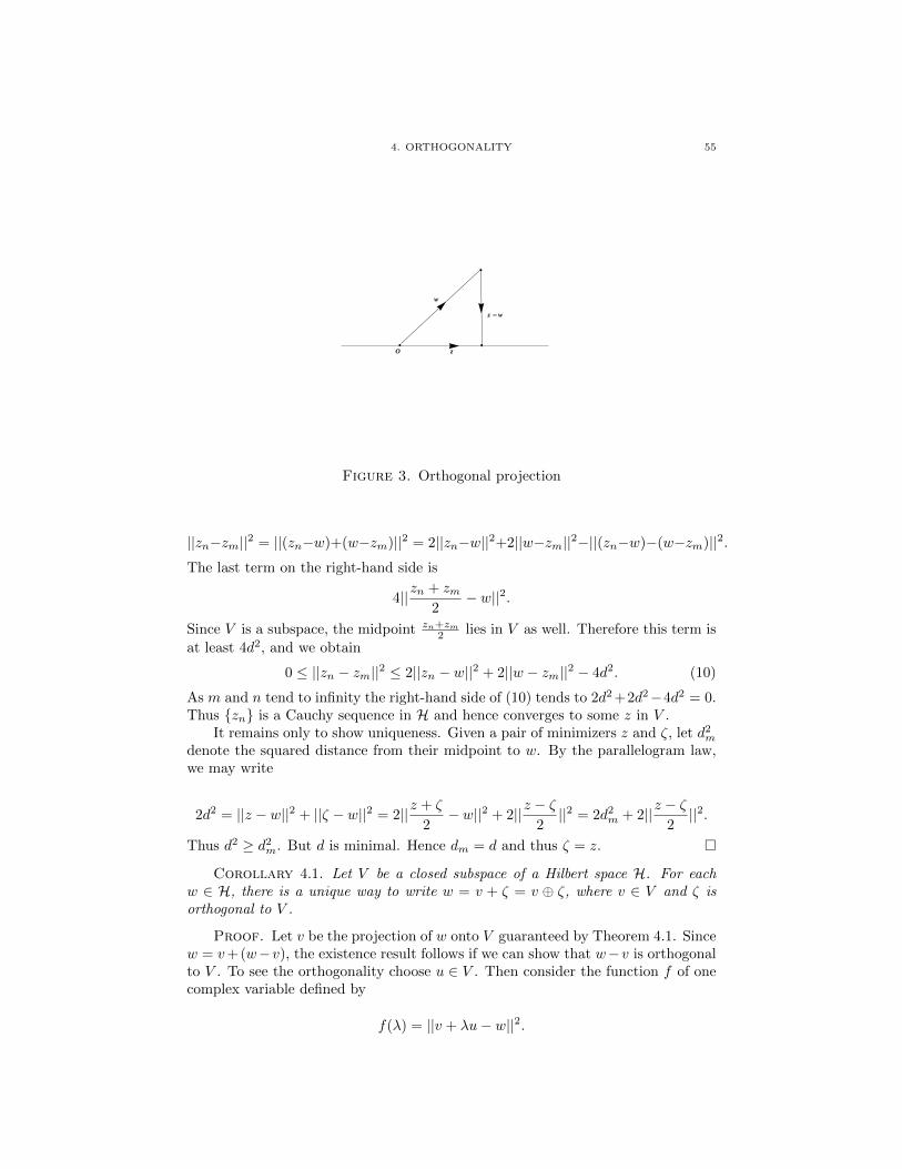
4. ORTHOGONALITY 55
O
w
z
z - w
Figure 3. Orthogonal projection
||zn−zm||2 = ||(zn−w)+(w−zm)||2 = 2||zn−w||2+2||w−zm||2−||(zn−w)−(w−zm)||2.The last term on the right-hand side is
4||zn + zm2
− w||2.
Since V is a subspace, the midpoint zn+zm2 lies in V as well. Therefore this term is
at least 4d2, and we obtain
0 ≤ ||zn − zm||2 ≤ 2||zn − w||2 + 2||w − zm||2 − 4d2. (10)
As m and n tend to infinity the right-hand side of (10) tends to 2d2 +2d2−4d2 = 0.Thus zn is a Cauchy sequence in H and hence converges to some z in V .
It remains only to show uniqueness. Given a pair of minimizers z and ζ, let d2m
denote the squared distance from their midpoint to w. By the parallelogram law,we may write
2d2 = ||z − w||2 + ||ζ − w||2 = 2||z + ζ
2− w||2 + 2||z − ζ
2||2 = 2d2
m + 2||z − ζ2||2.
Thus d2 ≥ d2m. But d is minimal. Hence dm = d and thus ζ = z.
Corollary 4.1. Let V be a closed subspace of a Hilbert space H. For eachw ∈ H, there is a unique way to write w = v + ζ = v ⊕ ζ, where v ∈ V and ζ isorthogonal to V .
Proof. Let v be the projection of w onto V guaranteed by Theorem 4.1. Sincew = v+(w−v), the existence result follows if we can show that w−v is orthogonalto V . To see the orthogonality choose u ∈ V . Then consider the function f of onecomplex variable defined by
f(λ) = ||v + λu− w||2.
56 2. HILBERT SPACES
By Theorem 4.1, f achieves its minimum at λ = 0. Therefore for all λ
0 ≤ f(λ)− f(0) = 2Re〈v − w, λu〉+ |λ|2||u||2. (11)
We claim that (11) forces 〈v − w, u〉 = 0. Granted the claim, we note that u is anarbitrary element of V . Therefore v − w is orthogonal to V , as required.
To prove the claim, thereby completing the proof of existence, we note that〈v−w, u〉 is the (partial) derivative of f with respect to λ at 0, and hence vanishesat a minimum of f .
The uniqueness assertion is easy; we use the notation for orthogonal sum. Sup-pose w = v ⊕ ζ = v′ ⊕ ζ ′, as in the statement of the Corollary. Then
0 = w − w = (v − v′)⊕ (ζ − ζ ′)from which we obtain v = v′ and ζ = ζ ′.
Corollary 4.2. Let V be a closed subspace of a Hilbert space H. For eachw ∈ H, let Pw denote the unique z ∈ V guaranteed by Theorem 4.1; Pw is also thev guaranteed by Corollary 4.1. Then the mapping w → P (w) is a bounded lineartransformation satisfying P 2 = P . Thus P is a projection.
Proof. Both the existence and uniqueness assertions in Corollary 4.1 matterin this proof. Given w1 and w2 in H, by existence we may write w1 = Pw1 ⊕ ζ1and w2 = Pw2 ⊕ ζ2. Adding gives
w1 + w2 = (Pw1 ⊕ ζ1) + (Pw2 ⊕ ζ2) = (Pw1 + Pw2)⊕ (ζ1 + ζ2). (12)
The uniqueness assertion and (12) show that Pw1+Pw2 is the unique element ofV corresponding to w1 +w2 guaranteed by Corollary 4.1; by definition this elementis P (w1 + w2). By uniqueness Pw1 + Pw2 = P (w1 + w2), and P is additive. In asimilar fashion we write w = Pw ⊕ ζ and hence
cw = c(Pw)⊕ cζ.
Again by uniqueness, c(Pw) must be the unique element corresponding to cw guar-anteed by Corollary 4.1; by definition this element is P (cw). Hence cP (w) = P (cw).We have now shown that P is linear.
To show that P is bounded, we note from the Pythagorean theorem that||w||2 = ||Pw||2 + ||ζ||2, and hence ||Pw|| ≤ ||w||.
Finally we show that P 2 = P . For z = v⊕ ζ, we have P (z) = v = v⊕ 0. Hence
P 2(z) = P (P (z)) = P (v ⊕ 0) = v = P (z).
Theorem 4.1 and its consequences are among the most powerful results in thebook. The theorem guarantees that we can solve a minimization problem in diverseinfinite-dimensional settings, and it implies the Riesz representation lemma.
Fix w ∈ H, and consider the function from H to C defined by Lz = 〈z, w〉.Then L is a bounded linear functional. The linearity is evident. The boundednessfollows from the Cauchy-Schwarz inequality; setting C = ||w|| guarantees that|L(z)| ≤ C||z|| for all z ∈ H.

4. ORTHOGONALITY 57
The following fundamental result of F. Riesz characterizes bounded linear func-tionals on a Hilbert space; a bounded linear functional must be given by an innerproduct. The proof relies on projection onto a closed subspace.
Theorem 4.2 (Riesz Lemma). Let H be a Hilbert space and suppose that L ∈L(H,C). Then there is a unique w ∈ H such that
L(z) = 〈z, w〉for all z ∈ H. The norm ||L|| of the linear transformation L equals ||w||.
Proof. Since L is bounded, its nullspace N (L) is closed. If N (L) = H, wetake w = 0 and the result is true.
Suppose that N (L) is not H. Theorem 4.1 implies that there is a nonzeroelement w0 orthogonal to N (L). To find such a w0, choose any nonzero elementnot in N (L) and subtract its orthogonal projection onto N (L).
Let z be an arbitrary element of H. For a complex number α we can write
z = (z − αw0) + αw0.
Note that L(z − αw0) = 0 if and only if α = L(z)L(w0) . For each z we therefore let
αz = L(z)L(w0) .
Since w0 is orthogonal to N (L), computing the inner product with w0 yields
〈z, w0〉 = αz||w0||2 =L(z)
L(w0)||w0||2. (13)
From (13) we see that
L(z) = 〈z, w0
||w0||2L(w0)〉
and the existence result is proved. An explicit formula for w holds:
w =w0
||w0||2L(w0).
The uniqueness for w is immediate from the test we mentioned earlier. If〈ζ, w − w′〉 vanishes for all ζ, then w − w′ = 0.
It remains to show that ||L|| = ||w||. The Cauchy-Schwarz inequality yields
||L|| = sup||z||=1
|〈z, w〉| ≤ ||w||.
Choosing w||w|| for z yields
||L|| ≥ |L(w
||w||)| = 〈w,w〉
||w||= ||w||.
Combining the two inequalities shows that ||L|| = ||w||.
Exercise 4.1. Fix w with w 6= 0. Define P (v) by
P (v) =〈v, w〉||w||2
w.
Verify that P 2 = P .

58 2. HILBERT SPACES
Exercise 4.2. A sequence fn in a Hilbert space H converges weakly to f if,for each g ∈ H, the sequence 〈fn, g〉 converges to 〈f, g〉. Put H = L2([0, 2π]).Put fn(x) = sin(nx). Show that fn converges weakly to 0 but does not convergeto 0.
Exercise 4.3. (Harder) Let fn be a bounded sequence in a Hilbert spaceH. Show that fn has a weakly convergent subsequence.
Exercise 4.4. A hyperplane inH is a level set of a non-trivial linear functional.Assume that w 6= 0. Find the distance between the parallel hyperplanes given by〈z, w〉 = c1 and 〈z, w〉 = c2.
Exercise 4.5. Let b = bj be a sequence of complex numbers, and supposethere is a positive number C such that∣∣∣∣∣∣
∞∑j=1
ajbj
∣∣∣∣∣∣ ≤ C(
∞∑j=1
|aj |2)12
for all a ∈ l2. Show that b ∈ l2 and that∑|bj |2 ≤ C2. Suggestion: Consider the
map that sends a to∑ajbj .
5. Orthonormal expansion
We continue our general discussion of Hilbert spaces by studying orthonormalexpansions. The simplest example comes from basic physics. Let v = (a, b, c) be apoint or vector in R3. Physicists write v = ai + bj + ck, where i, j,k are mutuallyperpendicular vectors of unit length. Mathematicians write the same equation asv = ae1 + be2 + ce3; here e1 = (1, 0, 0) = i, e2 = (0, 1, 0) = j, and e3 = (0, 0, 1) = k.This equation expresses v in terms of an orthonormal expansion:
ae1 + be2 + ce3 = (a, b, c) = v = 〈v, e1〉e1 + 〈v, e2〉e2 + 〈v, e3〉e3.
Orthonormal expansion in a Hilbert space abstracts this idea. Fourier seriesprovide the basic example, where the functions x→ einx are analogous to mutuallyperpendicular unit vectors.
We assume here that a Hilbert space is separable. This term means that theHilbert space has a countable dense set; separability implies that the orthonormalsystems we are about to define are either finite or countably infinite sets. All thespecific Hilbert spaces mentioned or used in this book are separable. Some of theproofs given tacitly use separability even when the result holds more generally.
Definition 5.1. Let S = zn be a finite or countably infinite collection ofelements in a Hilbert space H. We say that S is an orthonormal system in H if, foreach n we have ||zn||2 = 1, and for each n,m with n 6= m, we have 〈zn, zm〉 = 0.We say that S is a complete orthonormal system if, in addition, 〈z, zn〉 = 0 for alln implies z = 0.
Proposition 5.1 (Bessel’s inequality). Let S = zn be a countably infiniteorthonormal system in H. For each z ∈ H we have
∞∑n=1
|〈z, zn〉|2 ≤ ||z||2. (14)

5. ORTHONORMAL EXPANSION 59
Proof. Choose z ∈ H. By orthonormality, for each positive integer N we have
0 ≤ ||z −N∑n=1
〈z, zn〉zn||2 = ||z||2 −N∑n=1
|〈z, zn〉|2. (15)
Define a sequence of real numbers rN = rN (z) by
rN =
N∑n=1
|〈z, zn〉|2.
By (15), rN is bounded above by ||z||2 and nondecreasing. Therefore it has a limitr = r(z). Bessel’s inequality follows.
Proposition 5.2 (Best approximation lemma). Let S = zn be an orthonor-mal system (finite or countable) in H. Let V be the span of S. Then, for eachz ∈ H and each w ∈ V ,
||z −∑〈z, zn〉zn|| ≤ ||z − w||.
Proof. The expression∑〈z, zn〉zn equals the orthogonal projection of z onto
V . Hence the result follows from Theorem 4.1.
The limit r(z) of the sequence in the proof of Bessel’s inequality equals ||z||2for each z if and only if the orthonormal system S is complete. This statement isthe content of the following fundamental theorem. In general r(z) is the squarednorm of the projection of z onto the span of the zj .
Theorem 5.1 (Orthonormal Expansion). An orthonormal system S = zn iscomplete if and only if, for each z ∈ H, we have
z =∑n
〈z, zn〉zn. (16)
Proof. The cases where S is a finite set or where H is finite-dimensional areevident. Assume then that H is infinite-dimensional and S is a countably infiniteset. We first verify that the series in (16) converges. Fix z ∈ H. Put
TN =
N∑n=1
〈z, zn〉zn
and, for N > M , observe that
||TN − TM ||2 = ||N∑
n=M+1
〈z, zn〉zn||2 =
N∑n=M+1
|〈z, zn〉|2 = rN − rM . (17)
Since rN converges, it is a Cauchy sequence of real numbers. By (17), TN is aCauchy sequence in H. Since H is complete, TN converges to some element w of H,and w =
∑〈z, zn〉zn. Note that 〈w, zn〉 = 〈z, zn〉 for each n, so z −w is orthogonal
to each zn.We can now establish both implications. Suppose first that S is a complete
system. Since z −w is orthogonal to each zn, we have z −w = 0. Thus (16) holds.Conversely, suppose that (16) holds. To show that S is a complete system, we
60 2. HILBERT SPACES
assume that 〈z, zn〉 = 0 for all n, and hope to show that z = 0. This conclusionfollows immediately from (16).
Exercise 5.1. Verify (15).
Exercise 5.2. Let H = L2([−1, 1]) with the usual inner product. Apply theGram-Schmidt process (see [G]) to the polynomials 1, x, x2, x3.
Exercise 5.3. Assume H is infinite-dimensional. Show that a sequence oforthonormal vectors does not converge, but does converge weakly to 0. (See Exercise4.2 for the definition of weak convergence.)
6. Polarization
In a Hilbert space we can recover the Hermitian inner product from the squarednorm. In addition, for each linear operator L we can recover 〈Lz,w〉 for all z, wfrom knowing 〈Lz, z〉 for all z. See Theorem 6.1. The corresponding result for realvector spaces with inner products fails.
To introduce these ideas, let m be an integer with m ≥ 2. Recall, for z 6= 1,the sum of the finite geometric series:
1 + z + z2 + · · ·+ zm−1 =1− zm
1− z.
When z is an m-th root of unity, the sum is zero. A primitive m-th root of unityis a complex number ω such that ωm = 1, but no smaller positive power equals 1.The set of powers ωj for j = 0, 1, . . . ,m− 1 forms a cyclic group Γ of order m.
Let ω be a primitive m-th root of unity and consider averaging the m complexnumbers γ||z + γζ||2 as γ varies over Γ. Since each group element is a power of ω,this average equals
1
m
m−1∑j=0
ωj ||z + ωjζ||2.
The next proposition gives a simple expression for the average.
Proposition 6.1 (Polarization identities). Let ω be a primitive m-th root ofunity. For m ≥ 3 we have
〈z, ζ〉 =1
m
m−1∑j=0
ωj ||z + ωjζ||2. (18)
For m = 2 the right-hand side of (18) equals 2Re〈z, ζ〉.
Proof. We prove (18) below when m = 4, leaving the general case to thereader.
For m ≥ 3, each identity in (18) expresses the inner product in terms of squarednorms. It is both beautiful and useful to recover the inner product from the squarednorm. The special case of (18) where m = 4 arises often. We state it explicitly andprove it.
4〈z, w〉 = ||z + w||2 + i||z + iw||2 − ||z − w||2 − i||z − iw||2. (19)

6. POLARIZATION 61
To verify (19), observe that expanding the squared norms gives both equations:
4Re〈z, w〉 = ||z + w||2 − ||z − w||2
4Re〈z, iw〉 = ||z + iw||2 − ||z − iw||2.Observe for ζ ∈ C that Re(−iζ) = Im(ζ). Thus multiplying the second equationby i, using i(−i) = 1, and then adding the two equations, gives (19).
In addition to polarizing the inner product, we often polarize expressions in-volving linear transformations.
Theorem 6.1 (Polarization identities for operators). Let L ∈ L(H). Supposeω is a primitive m-th root of unity.
1) For m ≥ 3 we have
〈Lz, ζ〉 =1
m
m−1∑j=0
ωj〈L(z + ωjζ), z + ωjζ〉. (20)
2) For m = 2 we have
〈Lz, ζ〉+ 〈Lζ, z〉 =1
2(〈L(z + ζ), z + ζ〉 − 〈L(z − ζ), z − ζ〉). (21)
3) Suppose in addition that 〈Lv, v〉 is real for all v ∈ H. Then, for all z and ζ,
〈Lz, ζ〉 = 〈Lζ, z〉.4) Suppose 〈Lz, z〉 = 0 for all z. Then L = 0.
Proof. To prove (20) and (21), expand each 〈L(z + ωjζ), z + ωjζ〉 using thelinearity of L and the defining properties of the inner product. Collect similar terms,and use the above comment about roots of unity. For m ≥ 3, all terms inside thesum cancel except for m copies of 〈Lz, ζ〉. The result gives (20). For m = 2, thecoefficient of 〈Lζ, z〉 does not vanish, and we obtain (21). Thus statements 1) and2) hold.
To prove the third statement, we apply the first for some m with m ≥ 3 andωm = 1; the result is
〈Lz, ζ〉 =1
m
m−1∑j=0
ωj〈L(z + ωjζ), z + ωjζ〉 =1
m
m−1∑j=0
ωj〈L(ωm−jz + ζ), ωm−jz + ζ〉.
(22)Change the index of summation by setting l = m − j. Also observe that
ω−1 = ω. Combining gives the first equality in (23) below. Finally, because 〈Lv, v〉is real, and ω0 = ωm we obtain the second equality in (23):
〈Lz, ζ〉 =1
m
m∑l=1
ωl〈L(ζ + ωlz), ζ + ωlz〉 = 〈Lζ, z〉. (23)
We have now proved the third statement.The fourth statement follows from (20); each term in the sum on the right-hand
side of (20) vanishes if 〈Lw,w〉 = 0 for all w. Thus 〈Lz, ζ〉 = 0 for all ζ. HenceLz = 0 for all z, and thus L = 0.

62 2. HILBERT SPACES
The reader should compare these results about polarization with our earlierresults about Hermitian symmetric polynomials.
Exercise 6.1. Give an example of a linear map of R2 such that 〈Lu, u〉 = 0for all u but L is not 0.
7. Adjoints and unitary operators
Let I denote the identity linear transformation on a Hilbert space H. LetL ∈ L(H). Then L is called invertible if there is a bounded linear mapping T suchthat LT = TL = I. If such a T exists, then T is unique, and written L−1. Wewarn the reader (see the exercises) that, in infinite dimensions, LT = I does notimply that L is invertible. When L is bounded, injective, and surjective, the usualset-theoretic inverse is also linear and bounded.
Given a bounded linear mapping L, the adjoint of L is written L∗. It is definedas follows. Fix v ∈ H. Consider the map u → 〈Lu, v〉 = φv(u). It is obviously alinear functional. It is also continuous because
|φv(u)| = |〈Lu, v〉| ≤ ||Lu|| ||v|| ≤ ||u|| ||L|| ||v|| = c||u||, (24)
where the constant c is independent of u. By Theorem 4.2, there is a unique wv ∈ Hfor which φv(u) = 〈u,wv〉. We denote wv by L∗v. It is easy to prove that L∗ isitself a bounded linear mapping on H, called the adjoint of L.
The following properties of adjoints are left as exercises.
Proposition 7.1. Let L, T ∈ L(H). The following hold:
(1) L∗ : H → H is linear.(2) L∗ is bounded. (In fact ||L∗|| = ||L||.)(3) (L∗)∗ = L.(4) 〈Lu, v〉 = 〈u, L∗v〉 for all u, v.(5) (LT )∗ = T ∗L∗.
Proof. See Exercise 7.1.
Exercise 7.1. Prove Proposition 7.1.
Definition 7.1. A bounded linear transformation L on a Hilbert space H iscalled Hermitian or self adjoint if L = L∗. It is called unitary if it is invertible andL∗ = L−1.
The following simple but beautiful result characterizes unitary transformations.
Proposition 7.2. The following are equivalent for L ∈ L(H).
(1) L is surjective and preserves norms: ||Lu||2 = ||u||2 for all u.(2) L is surjective and preserves inner products: 〈Lu,Lv〉 = 〈u, v〉 for all u, v.(3) L is unitary: L∗ = L−1.
Proof. If L ∈ L(H), then 〈Lu,Lv〉 = 〈u, v〉 for all u, v if and only if 〈u, L∗Lv〉 =〈u, v〉 for all u, v and thus if and only if 〈u, (L∗L − I)v〉 = 0 for all u, v. This laststatement holds if and only if (L∗L − I)v = 0 for all v. Thus L∗L = I. If L isalso surjective, then L∗ = L−1, and therefore the second and third statements areequivalent.
7. ADJOINTS AND UNITARY OPERATORS 63
The second statement obviously implies the first. It remains to prove the subtlepoint that the first statement implies the second or third statement. We are given〈L∗Lz, z〉 = 〈z, z〉 for all z. Hence 〈(L∗L− I)z, z〉 = 0. By part 4 of Theorem 6.1,L∗L − I = 0, and the second statement holds. If L is also surjective, then L isinvertible and hence unitary.
The equivalence of the first two statements does not require L to be surjec-tive. See the exercises for examples where L preserves inner products but L is notsurjective and hence not unitary.
Exercise 7.2. If L : Cn → Cn and L = L∗, what can we conclude about thematrix of L with respect to the usual basis (1, 0, . . . , 0), ..., (0, 0, . . . , 1)?
Exercise 7.3. Suppose U is unitary and Uz = λz for z 6= 0. Prove that|λ| = 1. Suppose L is Hermitian and Lz = λz for z 6= 0. Prove that λ is real.
Exercise 7.4. Let L : l2 → l2 be defined by
L(z1, z2, . . . ) = (0, z1, z2, . . . ).
Show that ||Lz||2 = ||z||2 for all z but that L is not unitary.
Exercise 7.5. Give an example of a bounded linear L : H → H that is injectivebut not surjective, and an example that is surjective but not injective.
Exercise 7.6. Let V be the vector space of all polynomials in one variable.Let D denote differentiation, and J denote integration (with integration constant0). Show that DJ = I but that JD 6= I. Explain.
Exercise 7.7. Assume L ∈ L(H). Show that L is a linear combination oftwo Hermitian operators. (Harder) Show that a Hermitian operator is a linearcombination of two unitary operators.
Exercise 7.8. Give an example of an operator L for which ||L2|| 6= ||L||2.Suppose L = L∗; show that ||L2|| = ||L||2.
We close this section with an interesting difference between real and complexvector spaces, related to inverses, polarization, and Exercise 6.1. The formula (*)below interests the author partly because, although no real numbers satisfy theequation, teachers often see it on exams.
Definition 7.2. A real vector space V admits a complex structure if there isa linear map J : V → V such that J2 = −I.
It is easy to show (Exercise 7.10) that a finite-dimensional real vector spaceadmits a complex structure if and only if its dimension is even. For example, thelinear transformation J : R2 → R2 corresponding to the complex structure is givenby the matrix
J =
(0 −11 0
).
Proposition 7.3. Let V be a vector space over R. Then there are invertiblelinear transformations A,B on V satisfying
(A+B)−1 = A−1 +B−1 (∗)if and only if V admits a complex structure.

64 2. HILBERT SPACES
Proof. Invertible A,B satisfying (*) exist if and only if
I = (A+B)(A−1 +B−1) = I +BA−1 + I +AB−1.
Put C = BA−1. The condition (*) is therefore equivalent to finding C such that0 = I + C + C−1, which is equivalent to 0 = I + C + C2. Suppose such C exists.Put J = 1√
3(I + 2C). Then we have
J2 =1
3(I + 2C)2 =
1
3(I + 4C + 4C2) =
1
3(−3I + 4(I + C + C2)) = −I.
Hence V admits a complex structure. Conversely, if V admits a complex structure,
then J exists with J2 = −I. Put C = −I+√
3J2 ; then I + C + C2 = 0.
Exercise 7.9. Explain the proof of Proposition 7.3 in terms of cube roots ofunity.
Exercise 7.10. Prove that a finite-dimensional real vector space with a com-plex structure must have even dimension. Hint: Consider the determinant of J .
8. A return to Fourier series
The specific topic of Fourier series motivated many of the abstract results aboutHilbert spaces and it provides one of the best examples of the general theory. Inreturn, the general theory clarifies the subject of Fourier series.
Let h be (Riemann) integrable on the circle and consider its Fourier series∑h(n)einx. Recall that its symmetric partial sums SN are given by
SN (h)(x) =
N∑n=−N
h(n)einx.
When h is sufficiently smooth, SN (h) converges to h. See for example Theorem 8.2.We show next that SN (h) converges to h in L2. Rather than attempting to proveconvergence at each point, this result considers an integrated form of convergence.
Theorem 8.1. Suppose f is integrable on the circle. Then ||SN (f)−f ||L2 → 0.
Proof. Given ε > 0 and an integrable f , we first approximate f to withinε2 in the L2 norm by a continuous function g. Then we approximate g by a trigpolynomial p to within ε
2 . See below for details. These approximations yield
||f − p||L2 ≤ ||f − g||L2 + ||g − p||L2 <ε
2+ε
2= ε. (25)
Once we have found this p, we use orthogonality as in Theorem 4.1. Let N beat least as large as the degree of p. Let VN denote the (2N + 1)-dimensional (henceclosed) subspace spanned by the functions einx for |n| ≤ N . By Theorem 4.1, thereis a unique element w of VN minimizing ||f − w||L2 . That w is the partial sumSN (f), namely the orthogonal projection of f onto VN .
By Proposition 5.2, we have
||f − SN (f)||L2 ≤ ||f − p||L2 (26)
for all elements p of VN . Take p to be the polynomial in (25) and take N at leastthe degree of p. Combining (26) and (25) then gives
||f − SN (f)||L2 ≤ ||f − p||L2 ≤ ||f − g||L2 + ||g − p||L2 < ε. (27)
8. A RETURN TO FOURIER SERIES 65
It therefore suffices to verify that the two above approximations are valid.Given f integrable, by Lemma 7.1 of Chapter 1 we can find a continuous g suchthat sup(|g|) ≤ sup(|f |) = M and such that ||f −g||L1 is as small as we wish. Since
||f−g||2L2 =1
2π
∫ 2π
0
|f−g|2dx ≤ sup(|f − g|)2π
∫ 2π
0
|f−g|dx ≤ 2M ||f−g||L1 , (28)
we may choose g to bound the expression in (28) by ε2 .
Now g is given and continuous on the circle. By Corollary 10.2 of Chapter 1,there is a trig polynomial p such that ||g − p||L∞ < ε
2 . Therefore
||g − p||2L2 =1
2π
∫ 2π
0
|g(x)− p(x)|2dx ≤ ||g − p||2L∞ .
Hence ||g − p||L2 < ε2 as well. We have established both approximations used in
(25) and hence the conclusion of the theorem.
Corollary 8.1 (Parseval’s formula). If f is integrable on the circle, then
∞∑−∞|f(n)|2 = ||f ||2L2 . (29)
Proof. By the orthonormality properties of the functions x→ einx, f−SN (f)is orthogonal to VN . By the Pythagorean theorem, we have
||f ||2L2 = ||f − SN (f)||2L2 + ||SN (f)||2L2 = ||f − SN (f)||2L2 +
N∑−N|f(n)|2. (30)
Letting N tend to infinity in (30) and using Theorem 8.1 gives (29).
Corollary 8.2 (Riemann-Lebesgue lemma). If f is integrable on the circle,
then lim|n|→∞ f(n) = 0.
Proof. The series in (29) converges; hence its terms tend to 0.
Polarization has several applications to Fourier series. By (29), if f and g are
integrable on the circle, then∑|f |2 = ||f ||2L2 and similarly for g. It follows by
polarization that
〈f , g〉2 =
∞∑−∞
f(n)g(n) =1
2π
∫ 2π
0
f(x)g(x)dx = 〈f, g〉L2 . (31)
Corollary 8.3. If f and g are integrable on the circle, then (31) holds.
Corollary 8.4. The map f → F(f) from L2(S1) to l2 satisfies the relation
〈Ff,Fg〉2 = 〈f, g〉L2 .
The analogue of this corollary holds for Fourier transforms on R, Rn, or in evenmore abstract settings. Such results, called Plancherel theorems, play a crucial rolein extending the definition of Fourier transform to objects (called distributions)more general than functions. See Chapter 3.
Theorem 8.2. Suppose f is continuously differentiable on the circle. Then itsFourier series converges absolutely to f .

66 2. HILBERT SPACES
Proof. By Lemma 9.2 of Chapter 1, we have f(n) = f ′(n)in for n 6= 0. We first
apply the Parseval identity to the Fourier series for f ′, getting
1
2π
∫|f ′(x)|2dx =
∑|f ′(n)|2 =
∑n2|f(n)|2. (32)
Then we use the Cauchy-Schwarz inequality on∑|f(n)| to get∑
|f(n)| = |f(0)|+∑ 1
nn|f(n)| ≤ |f(0)|+ (
∑ 1
n2)
12 (∑
n2|f(n)|2)12 . (33)
By (32), the second sum on the right-hand side of (33) converges. The sum∑n 6=0
1n2
also converges and can be determined exactly using Fourier series. See Exercise 8.1.Since each partial sum is continuous and the partial sums converge uniformly,
the limit is continuous. By Corollary 12.2 of Chapter 1, the Fourier series convergesabsolutely to f .
Exercise 8.1. Compute the Fourier series for the function f defined by f(x) =
(π − x)2 on (0, 2π). Use this series to show that∑∞n=1
1n2 = π2
6 .
Exercise 8.2. Find∑∞n=1
(−1)n
n2 . Suggestion. Find the Fourier series for x2
on (−π, π).
9. Bernstein’s theorem
We continue by proving a fairly difficult result. We include it to illustratecircumstances more general than Theorem 8.2 in which Fourier series convergeabsolutely and uniformly.
Definition 9.1. Let f : S1 → C be a function and suppose α > 0. We saythat f satisfies a Holder condition of order α if there is a constant C such that
|f(x)− f(y)| ≤ C|x− y|α (34)
for all x, y. Sometimes we say f is Holder continuous of order α.
By the mean-value theorem from calculus, a differentiable function satisfies theinequality
|f(x)− f(y)| ≤ sup|f ′(t)| |x− y|.Hence, if f ′ is bounded, f satisfies a Holder condition with α = 1. Note also thata function satisfying (34) must be uniformly continuous.
Theorem 9.1. Suppose f is Holder continuous on the circle of order α, andα > 1
2 . Then the Fourier series for f converges absolutely and uniformly.
Proof. The Holder condition means that there is a constant C such thatinequality (34) holds. We must somehow use this condition to study∑
n∈Z
|f(n)|.
The remarkable idea here is to break up this sum into dyadic parts, and estimatedifferently in different parts. For p a natural number let Rp denote the set of n ∈ Zfor which 2p−1 ≤ |n| < 2p. Note that there are 2p integers in Rp. We have∑
n∈Z
|f(n)| = |f(0)|+∑p
∑n∈Rp
|f(n)|. (35)

9. BERNSTEIN’S THEOREM 67
In each Rp we can use the Cauchy-Schwarz inequality to write
∑n∈Rp
|f(n)| ≤
∑n∈Rp
|f(n)|2 1
2
(2p)12 . (36)
At first glance the factor 2p2 looks troublesome, but we will nonetheless show that
this series is convergent.Let gh be defined by gh(x) = f(x+ h)− f(x− h). The Holder condition gives
|gh(x)|2 ≤ C2|2h|2α = C ′|h|2α,
and integrating we obtain
||gh||2L2 ≤ C ′|h|2α.By the Parseval-Plancherel theorem (Corollary 8.1), for any h we have∑
n∈Z
|gh(n)|2 = ||gh||2L2 ≤ C ′|h|2α. (37)
Now we compute the Fourier coefficients of gh, relating them to f . Using thedefinition directly, we get
gh(n) =1
2π
∫ 2π
0
(f(x+ h)− f(x− h)) e−inxdx.
Changing variables in each term and recollecting gives
gh(n) =1
2π
∫ 2π
0
f(y)e−inyeinhdy − 1
2π
∫ 2π
0
f(y)e−inye−inhdy = 2isin(nh)f(n).
Hence we have
|gh(n)|2 = 4sin2(nh)|f(n)|2.Putting things together we obtain, with a new constant c,
sin2(nh)|f(n)|2 =1
4|gh(n)|2 ≤ 1
4
∑n
|gh(n)|2 ≤ c|h|2α. (38)
Also we have∑n∈Rp
|f(n)|2 =∑n∈Rp
|f(n)|2sin2(nh)1
sin2(nh)=∑n∈Rp
|gh(n)|2 1
4sin2(nh). (39)
Put h = π2p+1 . Then π
4 ≤ |n|h ≤π2 and hence 1
2 ≤ sin2(nh) ≤ 1. Using sin2(nh) ≥ 12
in (39), we get ∑n∈Rp
|f(n)|2 ≤ 1
2
∑n∈Rp
|gh(n)|2. (40)
For h = π2p+1 , we have
|gh(n)|2 ≤ C1|π
2p+1|2α ≤ C22−2αp. (41)
Combining (40), (41), and (36) (note the exponent 12 there) gives
68 2. HILBERT SPACES
∑n∈Z
|f(n)| = |f(0)|+∑p
∑n∈Rp
|f(n)| ≤ |f(0)|+ C2
∑p
2−αp2p2 . (42)
The series on the right-hand side of (42) is of the form∑xp where x = 2
1−2α2 .
If α > 12 , then |x| < 1 and this series converges.
The conclusion of the theorem fails if f satisfies a Holder condition of order 12 .
See [K].
10. Compact Hermitian operators
Fourier series give but one of many examples of orthonormal expansions. In thissection we establish the spectral theorem for compact Hermitian operators. Suchoperators determine complete orthonormal systems consisting of eigenvectors. Inthe next section we apply this result to Sturm-Liouville equations. These secondorder ordinary differential equations with homogeneous boundary conditions playeda major role in the historical development of operator theory and remain significantin current applied mathematics, engineering, and physics.
An operator on a Hilbert space is compact if it can be approximated (in norm)arbitrarily well by operators with finite-dimensional range. We mention this char-acterization for the intuition it provides. The precise definition, which also appliesin the context of complete normed vector spaces, involves subsequences. In olderliterature, compact operators are called completely continuous.
Definition 10.1. Suppose L ∈ L(H). Then L is compact if, whenever zn isa bounded sequence in H, then L(zn) has a convergent subsequence.
By the Bolzano-Weierstrass theorem (see Theorem 2.1 of the Appendix), eachbounded sequence in Cd has a convergent subsequence. Hence an operator withfinite-dimensional range must be compact. A constant multiple of a compact op-erator is compact. The sum of two compact operators is compact. We check inProposition 10.2 that the composition (on either side) of a compact operator with abounded operator is compact. On the other hand, the identity operator is compactonly when the Hilbert space is finite-dimensional. Proposition 10.5 gives one ofmany possible proofs of this last statement.
We will use the following simple characterization of compact operators. See[D1] for many uses of the method. The two statements in the proof are equivalent,with different values of ε. In the statement we write f for an element of H, toremind us that we are typically working on function spaces.
Proposition 10.1. Suppose L ∈ L(H). Then L is compact if (and only if), foreach ε > 0, there are compact operators Kε and Tε such that either of the following(equivalent) statements holds:
||Lf || ≤ ε||f ||+ ||Kεf ||||Lf ||2 ≤ ε||f ||2 + ||Tεf ||2.
Proof. Assuming the first inequality, we prove that L is compact. The proofassuming the second inequality is similar. Let fn be a bounded sequence; we mayassume that ||fn|| ≤ 1. For each positive integer m, we set ε = 1
m in the inequality.We obtain a sequence Lm of compact operators. Thus each sequence Lm(fn)has a convergent subsequence. By the Cantor diagonalization trick, there is a single

10. COMPACT HERMITIAN OPERATORS 69
subsequence fnk such that Lm(fnk) converges for all m. By the inequality, foreach m we have
||L(fnk)− L(fnl)|| = ||L(fnk − fnl)|| ≤ (1
m)||fnk − fnl ||+ ||Lm(fnk − fnl)||.
Given δ > 0, we can bound the first term by δ2 by choosing 1
m < δ4 . Since Lm(fnk)
converges, it is Cauchy; we can therefore bound the second term by δ2 by picking
nk and nl sufficiently large. Therefore the sequence L(fnk) is also Cauchy in H.Since H is complete, L(fnk) converges, and thus L is compact.
If we know that L is compact, then we may choose Kε or Tε equal to L. Thepoint of Proposition 10.1 is the converse statement. We can often prove compactnessby proving an inequality, instead of dealing with subsequences. We illustrate withseveral examples, which can of course also be proved using subsequences.
Proposition 10.2. Suppose L ∈ L(H) and L is compact. If M,T ∈ L(H),then ML and LT are compact.
Proof. That LT is compact follows directly from the definition of compact-ness. If zn is a bounded sequence, then Tzn also is, and hence L(Tzn) has aconvergent subsequence. Similarly, ML is compact.
That ML is compact can also be proved using Proposition 10.1 as follows.Given ε > 0, put ε′ = ε
1+||M || . Put K = ||M || L; then K is compact. We have
||MLz|| ≤ ||M || ||Lz|| ≤ ||M ||(ε′||z||+ ||Lz||) ≤ ε||z||+ ||Kz||.By Proposition 10.1, ML is also compact.
Proposition 10.3. Let Ln be a sequence of operators with limn ||Ln−L|| = 0.If each Ln is compact, then L is also compact.
Proof. Given ε > 0, we can find an n such that ||L−Ln|| < ε. Then we write
||Lf || ≤ ||(L− Ln)f ||+ ||Ln(f)|| ≤ ε||f ||+ ||Ln(f)||.The result therefore follows from Proposition 10.1.
A converse of Proposition 10.3 also holds; each compact operator is the limitin norm of a sequence of operators with finite-dimensional ranges. We can also useProposition 10.1 to prove the following result.
Theorem 10.1. Assume L ∈ L(H). If L is compact, then L∗ is compact.Furthermore, L is compact if and only if L∗L is compact.
Proof. See Exercise 10.3.
Exercise 10.1. (Small constant large constant trick) Given ε > 0, prove thatthere is a Cε > 0 such that
|〈x, y〉| ≤ ε||x||2 + Cε||y||2.
Exercise 10.2. Prove that the second inequality in Proposition 10.1 impliescompactness.
Exercise 10.3. Prove Theorem 10.1. Use Proposition 10.1 and Exercise 10.1to establish the if part of the implication.

70 2. HILBERT SPACES
Before turning to the spectral theorem for compact Hermitian operators, wegive one of the classical types of examples. The function K in this example is calledthe integral kernel of the operator T . Such integral operators arise in the solutionsof ordinary differential equations such as the Sturm-Liouville equation.
Proposition 10.4. Let H = L2([a, b]). Assume that (x, t) → K(x, t) is con-tinuous on [a, b]× [a, b]. Define an operator T on H by
Tf(x) =
∫ b
a
K(x, t)f(t)dt.
Then T is compact. (The conclusion holds under weaker assumptions on K.)
Proof. Let fn be a bounded sequence in L2([a, b]). The following estimatefollows from the Cauchy-Schwarz inequality:
|T (fn)(x)− T (fn)(y)|2 ≤ sup|K(x, t)−K(y, t)|2||fn||2L2 .
Since K is continuous on the compact set [a, b]× [a, b], it is uniformly continuous.It follows that the sequence T (fn) is equi-continuous and uniformly bounded.By the Arzela-Ascoli theorem, there is a subsequence of T (fn) that convergesuniformly. In particular this subsequence converges in L2. Hence, T (fn) has aconvergent subsequence, and thus T is compact.
Exercise 10.4. Suppose that the integral kernel in Proposition 10.4 satisfies∫ ba|K(x, t)|dt ≤ C and
∫ ba|K(x, t)|dx ≤ C. Show that T ∈ L(H) and that ||T || ≤ C.
A compact operator need not have any eigenvalues or eigenvectors.
Example 10.1. Let L : l2 → l2 be defined by
L(z1, z2, . . . ) = (0, z1,z2
2,z3
3, . . . ).
Think of L as given by an infinite matrix with sub-diagonal entries 1, 12 ,
13 , . . . .
Then L is compact but has no eigenvalues.
Exercise 10.5. Verify the conclusions of Example 10.1.
Compact Hermitian operators, however, have many eigenvectors. In fact, bythe spectral theorem, there is a complete orthonormal system of eigenvectors.Before proving the spectral theorem, we note two easy results about eigenvectorsand eigenvalues.
Proposition 10.5. An eigenspace of a compact operator corresponding to anon-zero eigenvalue must be finite-dimensional.
Proof. Assume that L is compact and L(zj) = λzj for a sequence of orthogo-nal unit vectors zj . Since L is compact, L(zj) = λzj has a convergent subsequence.If λ 6= 0, then zj has a convergent subsequence. But no sequence of orthogonal unitvectors can converge. Thus λ = 0.
Proposition 10.6. The eigenvalues of a Hermitian operator are real and theeigenvectors corresponding to distinct eigenvalues are orthogonal.

10. COMPACT HERMITIAN OPERATORS 71
Proof. Assume Lf = λf and f 6= 0. We then have
λ||f ||2 = 〈Lf, f〉 = 〈f, L∗f〉 = 〈f, Lf〉 = 〈f, λf〉 = λ||f ||2.
Since ||f ||2 6= 0, we conclude that λ = λ.The proof of the second statement amounts to polarizing the first. Thus we
suppose Lf = λf and Lg = µg where λ 6= µ. We have, as µ is real,
λ〈f, g〉 = 〈Lf, g〉 = 〈f, Lg〉 = µ〈f, g〉.Hence 0 = (λ− µ)〈f, g〉 and the second conclusion follows.
Proposition 10.7. Suppose L ∈ L(H) is Hermitian. Then
||L|| = sup||z||=1
|〈Lz, z〉|. (43)
Proof. Let α equal the right-hand side of (43). We prove both inequalities:α ≤ ||L|| and ||L|| ≤ α. Since |〈Lz, z〉| ≤ ||Lz|| ||z||, we see that
α = sup||z||=1
|〈Lz, z〉| ≤ sup||z||=1
||Lz|| = ||L||.
The opposite inequality is harder. It uses the polarization identity (21) and theparallelogram law (9). We first note, by Theorem 6.1, that α = 0 implies L = 0.Hence we may assume α 6= 0. Since L is Hermitian, it follows that
〈Lz,w〉 = 〈z, Lw〉 = 〈Lw, z〉.Applying this equality in (21), we obtain, for all z, w,
4Re〈Lz,w〉 = 〈L(z + w), z + w〉 − 〈L(z − w), z − w〉.Using 〈Lζ, ζ〉 ≤ α||ζ||2 and the parallelogram law, we obtain
4Re〈Lz,w〉 ≤ α(||z + w||2 + ||z − w||2) = 2α(||z||2 + ||w||2). (44)
Set w = Lzα in (44) to get
4||Lz||2
α≤ 2α(||z||2 +
||Lz||2
α2).
Simplifying shows that this inequality is equivalent to 2 ||Lz||2
α ≤ 2α||z||2, which
implies ||Lz||2 ≤ α2||z||2. Hence ||L|| ≤ α.
Theorem 10.2 (Spectral Theorem). Suppose L ∈ L(H) is compact and Her-mitian. Then there is a complete orthonormal system consisting of eigenvectors ofL. Each eigenspace corresponding to a non-zero eigenvalue is finite-dimensional.
Proof. The conclusion holds if L is the zero operator; we therefore ignore thiscase and assume ||L|| > 0.
The first fact needed is that there is an eigenvalue λ with |λ| = ||L||. Note also,since L is Hermitian, that in this case λ is real and thus λ = ±||L||. In the proofwe write α for ±||L||; in general only one of the two values works.
Because L is Hermitian, the subtle formula (43) for the norm of L holds. Welet zν be a sequence on the unit sphere such that |〈Lzν , zν〉| converges to ||L||.Since L is compact, we can find a subsequence (still labeled zν) such that L(zν)converges to some w.
72 2. HILBERT SPACES
We will show that ||w|| = ||L|| and also that αzν converges to w. It followsthat zν converges to z = w
α . Then we have a unit vector z for which Lz = w = αz,and hence the first required fact will hold.
To see that ||w|| = ||L||, we prove both inequalities. Since the norm is contin-uous and ||zν || = 1, we obtain
||w|| = limν||Lzν || ≤ ||L||.
To see the other inequality, note that |〈Lzν , zν〉| is converging to ||L|| and L(zν) isconverging to w. Hence |〈w, zν〉| is converging to ||L|| as well. We then have
||L|| = limν|〈w, zν〉| ≤ ||w||.
Thus ||w|| = ||L||.Next we show that αzν converges to w. Consider the squared norm
||L(zν)− αzν ||2 = ||L(zν)||2 − α2Re〈Lzν , zν〉+ ||L||2.
The right-hand side converges to ||w||2−2||L||2+||L||2 = 0. Therefore the left-handside converges to 0 as well, and hence w = lim(αzν). Thus zν itself converges toz = w
α . Finally
L(z) = lim(L(zν)) = w = αz.
We have found an eigenvector z with eigenvalue α = ±||L||. By Proposition 10.5,the eigenspace Eα corresponding to α is finite-dimensional and thus a closed sub-space of H.
Once we have found one eigenvalue λ1, we consider the orthogonal complementE⊥λ1
of the eigenspace Eλ1. Then E⊥λ1
is invariant under L, and the restrictionof L to this subspace remains compact and Hermitian. We repeat the procedure,obtaining an eigenvalue λ2. The eigenspaces Eλ1 and Eλ2 are orthogonal. Con-tinuing in this fashion, we obtain a non-increasing sequence of (absolute values of)eigenvalues and corresponding eigenvectors. Each eigenspace is finite-dimensionaland the eigenspaces are orthogonal. We normalize the eigenvectors to have norm 1;hence there is a bounded sequence zj of eigenvectors. By compactness L(zj)has a convergent subsequence. Since L(zj) = λjzj , also λjzj has a convergentsubsequence. A sequence of orthonormal vectors cannot converge; the subsequencecannot be eventually constant because each eigenspace is of finite dimension. Theonly possibility is that the eigenvalues λj are tending to 0.
Finally we establish completeness. Let M denote a maximal collection of or-thonormal eigenvectors, including those with eigenvalue 0. Let Pn denote the pro-jection onto the span of the first n eigenvectors. We obtain
Pn(ζ) =
n∑j=1
〈ζ, zj〉zj .
Therefore
||L(Pn(ζ))− L(ζ)|| ≤ max(j≥n+1)|λj | ||ζ||. (45)
Since the eigenvalues tend to zero, (45) shows that L(Pn(ζ)) converges to L(ζ).Hence we obtain the orthonormal expansion for w in the range R(L) of L:
w = L(ζ) =
∞∑j=1
〈ζ, zj〉λjzj . (46)
11. STURM-LIOUVILLE THEORY 73
The nullspace N (L) is the eigenspace corresponding to eigenvalue 0, and henceany element of N (L) has an expansion in terms of vectors in M . Finally, for anybounded linear map L, the space N (L)⊕R(L∗) is dense in H. If also L = L∗, thenN (L) ⊕R(L) is dense. Therefore 0 is the only vector orthogonal to M , and M iscomplete.
Exercise 10.6. Try to give a different proof of (43). (In finite dimensions onecan use Lagrange multipliers.)
Exercise 10.7. Show that L∗L is compact and Hermitian if L is compact.
We close this section with a few words about unbounded operators. This termrefers to linear mappings, defined on dense subsets of a Hilbert space, but notcontinuous.
Suppose D is a dense subset of a Hilbert space H and L is defined and linearon D. If L were continuous, then L would extend to a linear mapping on H. Manyimportant operators are not continuous. Differentiation d
dx is defined and linear on
a dense set in L2([0, 2π]), but it is certainly not continuous. For example, einx
in converges to 0 in L2, but d
dx ( einx
in ) = einx, whose L2 norm equals 1 for each n. Toapply Hilbert space methods to differential operators, we must be careful.
Let L : D(L) ⊂ H → H be an unbounded operator. The domain D(L∗) ofthe adjoint of L is the set of v ∈ H such that the mapping u → 〈Lu, v〉 is acontinuous linear functional. By the Riesz Lemma, there is then a unique w suchthat 〈Lu, v〉 = 〈u,w〉. We then put L∗(v) = w. To say that an unbounded operatorL is self-adjoint or Hermitian means that D(L) = D(L∗) and the two maps agreethere. It often happens, with a given definition of D(L), that L∗ agrees with Lon D(L), but L is not self-adjoint. One must increase the domain of L, therebydecreasing the domain of L∗, until these domains are equal, before one can usewithout qualification the words self-adjoint or Hermitian.
Exercise 10.8. (Subtle) Put L = i ddx on the subspace of differentiable func-
tions f in L2([0, 1]) for which f(0) = f(1) = 0. Show that 〈Lf, g〉 = 〈f, Lg〉, butthat L is not Hermitian. Can you state precisely a domain for L making it Hermit-ian? Comment: Look up the term absolutely continuous and weaken the boundarycondition.
11. Sturm-Liouville theory
Fourier series provide the most famous example of orthonormal expansion, butmany other orthonormal systems arise in applied mathematics and engineering. Weillustrate by considering certain differential equations known as Sturm-Liouvilleequations. Mathematicians from the 19-th century were well-aware that manyproperties of the functions sine and cosine have analogues when these functionsare replaced by linearly independent solutions of a second-order linear ordinarydifferential equation. In addition to orthonormal expansions, certain oscillationissues generalize as well. We prove the Sturm separation theorem, an easy result,to illustrate this sort of generalization, before we turn to the more difficult matterof orthonormal expansion.
Consider a second order linear ordinary differential equation y′′+ qy′+ ry = 0.Here q and r are continuous functions of x. What can we say about the zeroes ofsolutions?

74 2. HILBERT SPACES
Π
Π 2 3 Π 2
1 2 3 4 5x
-1.0
-0.5
0.5
y
y''+ y=0
Figure 4. Sturm Separation
Theorem 11.1 (Sturm separation theorem). Let y1 and y2 be linearly indepen-dent (twice differentiable) solutions of y′′ + qy′ + ry = 0. Suppose that α < β andα, β are consecutive zeroes of y1. Then there is a unique x in the interval (α, β)with y2(x) = 0. Hence the zeroes of y1 and y2 alternate.
Proof. Consider the expression W (x) = y1(x)y′2(x) − y2(x)y′1(x), called theWronskian. We claim that it does not vanish. Assuming the claim, W has only onesign. We evaluate W at α and β, obtaining −y2(α)y′1(α) and −y2(β)y′1(β); theseexpressions must have the same sign. In particular, y′1 does not vanish at thesepoints. Also, the values y′1(α) and y′1(β) must have opposite signs because α andβ are consecutive zeroes of y1. Hence the values of y2(α) and y2(β) have oppositesigns. By the intermediate value theorem, there is an x in between α and β withy2(x) = 0. This x must be unique, because otherwise the same reasoning wouldfind a zero of y1 in between the two zeroes of y2. Since α and β are consecutivezeroes of y1, we would get a contradiction.
It remains to show that W is of one sign. We show more in Lemma 11.1.
Lemma 11.1. Suppose y1 and y2 both solve L(y) = y′′ + qy′ + ry = 0. Then y1
and y2 are linearly dependent if and only if W vanishes identically. Also y1 and y2
are linearly independent if and only if W vanishes nowhere.
Proof. Suppose first that W (x0) = 0. Since W (x0) is the determinant of thematrix of coefficients, the system of equations(
y1(x0) y2(x0)y′1(x0) y′2(x0)
)(c1c2
)=
(00
)has a non-trivial solution (c1, c2). Since L is linear, the function y = c1y1 + c2y2
also satisfies L(y) = 0. Since both y(x0) = y′(x0) = 0, this solution y is identically0. (See the paragraph after the proof.) Therefore the matrix equation holds at allx, the functions y1 and y2 are linearly dependent, and W is identically 0.

11. STURM-LIOUVILLE THEORY 75
Suppose next that W is never zero. Consider a linear combination c1y1 + c2y2
that vanishes identically. Then also c1y′1 + c2y
′2 vanishes identically, and hence(
y1 y2
y′1 y′2
)(c1c2
)=
(00
).
Since W is the determinant of the matrix here and W (x) 6= 0 for all x, the onlysolution is c1 = c2 = 0. Therefore y1 and y2 are linearly independent.
In the proof of Lemma 11.1, we used the following standard fact. The secondorder linear equation Ly = 0, together with initial conditions y(x0) and y′(x0), hasa unique solution. This result can be proved by reducing the second order equationto a first order system. Uniqueness for the first order system can be proved usingthe contraction mapping principle in metric spaces. See for example [Ro].
We now turn to the more sophisticated Sturm-Liouville theory. Consider thefollowing second-order differential equation on a real interval [a, b]. Here y is theunknown function; p, q, w are fixed real-valued functions, and the αj and βj arereal constants. These constants are subject only to the constraint that both (SL.1)and (SL.2) are non-trivial. In other words, neither α2
1 + α22 nor β2
1 + β22 is 0. This
problem is a boundary-value problem as values of y and y′ at both endpoints of theinterval [a, b] matter. The functions p′, q, w are continuous and the functions p andw are positive.
(py′)′ + qy + λwy = 0 (SL)
α1y(a) + α2y′(a) = 0 (SL.1)
β1y(b) + β2y′(b) = 0. (SL.2)
Remark 11.1. It is natural to ask how general the Sturm-Liouville equationis among second order equations. Consider any second order ODE of the formPy′′ + Qy′ + Ry = 0. We can always put it into the Sturm-Liouville form by thefollowing typical trick from ODE, called an integrating factor. We multiply theequation by an unknown function u, and figure out what u must be to put theequation in Sturm-Liouville form:
0 = uPy′′ + uQy′ + uRy = (py′)′ + ry.
To make this equation hold, we need uP = p and uQ = p′. Hence we requirep′
p = QP , which yields p = e
∫ QP . Hence, if we choose u = 1
P e∫ QP , we succeed.
The following lemma involving the Wronskian gets used in an important inte-gration by parts below and also implies that each eigenspace is one-dimensional.Note that the conclusion also holds if we replace g by g, because all the parametersin (SL), (SL.1), and (SL.2) are real.
Lemma 11.2. If f and g both satisfy (SL.1) and (SL.2), then
f(a)g′(a)− f ′(a)g(a) = f(b)g′(b)− f ′(b)g(b) = 0. (47)
Proof. Assume both f and g satisfy the conditions in (SL). We then can write(f(b) f ′(b)g(b) g′(b)
)(β1
β2
)=
(00
). (48)

76 2. HILBERT SPACES
and similarly for the values at a and the αj . Equations (SL.1) and (SL.2) are non-trivial; hence (48) and its analogue for a have non-trivial solutions, and each of thematrices (
f(a) f ′(a)g(a) g′(a)
)(f(b) f ′(b)g(b) g′(b)
)has a non-trivial nullspace. Hence each determinant vanishes.
Corollary 11.1. Suppose f and g both solve the same (SL) equation. Thenf and g are linearly dependent.
Proof. By Lemma 11.2, the two expressions in (47) vanish. But these ex-pressions are Wronskian determinants. By Lemma 11.1, the two solutions arelinearly independent if and only if their Wronskian determinant is (everywhere)non-zero.
Later we use one more fact about the Wronskian.
Lemma 11.3. Assume u, v both solve the Sturm-Liouville equation (py′)′+qy =0. Let W = uv′ − u′v. Then pW is constant. If u, v are linearly independent, thenthis constant is non-zero.
Proof. We want to show that (p(uv′−u′v))′ = 0. Computing the expression,without any assumptions on u, v, gives
p(uv′′ − u′′v) + p′(uv′ − u′v).
Since u and v satisfy the equation we also have
pu′′ + p′u′ + qu = 0
pv′′ + p′v′ + qv = 0.
Multiply the first equation by v, the second by u and then subtract. We get
p(u′′v − uv′′) + p′(u′v − uv′) = 0,
which is what we need. The last statement follows immediately from Lemma 11.1.
Each λ for which (SL) admits a non-zero solution is called an eigenvalue of theproblem, and each non-zero solution is called an eigenfunction corresponding to thiseigenvalue. The terminology is consistent with the standard notions of eigenvalueand eigenvector, as noted in Lemma 11.4 below. Corollary 11.1 thus says that theeigenspace corresponding to each eigenvalue is one-dimensional.
To connect the Sturm-Liouville setting with Fourier series, take p = 1, q = 0,and w = 1. We get the familiar equation
y′′ + λy = 0,
whose solutions are sines and cosines. For example, if the interval is [0, π], and weassume that (SL.1) and (SL.2) give y(0) = y(π) = 0, then the eigenvalues are m2
for positive integers m. The solutions are ym(x) = sin(mx).

11. STURM-LIOUVILLE THEORY 77
Sturm-Liouville theory uses the Hilbert space H = (L2([a, b]), w), consisting of(equivalence classes of) square-integrable measurable functions with respect to theweight function w. The inner product is defined by
〈f, g〉w =
∫ b
a
f(x)g(x)w(x)dx. (48)
Although the Sturm-Liouville situation is much more general than the equationy′′+λy = 0, the conclusions in the following theorem are remarkably similar to theresults we have proved about Fourier series.
Theorem 11.2. Consider the Sturm-Liouville equation (SL) with homogeneousboundary conditions. There is a countable collection of real eigenvalues λj tendingto ∞ with λ1 < λ2 < . . . . For each eigenvalue the corresponding eigenspace is one-dimensional. The corresponding eigenfunctions φj are orthogonal. After dividingeach φj by a constant, we assume that these eigenfunctions are orthonormal. Theseeigenfunctions form a complete orthonormal system for H. If f is continuouslydifferentiable on [a, b], then the series
∞∑j=1
〈f, φj〉wφj(x) (49)
converges to f(x) at each point of (a, b).
Proving this theorem is not easy, but we will give a fairly complete proof. Webegin by rephrasing everything in terms of an unbounded operator L on H. On anappropriate domain, L is defined by
L =−1
w
(d
dx
(pd
dx
)+ q
). (50)
The domain D(L) contains all twice continuously differentiable functions satisfyingthe (SL) boundary conditions. Eigenvalues of the Sturm-Liouville problem corre-spond to eigenvalues of this operator L.
Lemma 11.4. Equation (SL) is equivalent to Ly = λy.
Proof. Left to the reader.
Proposition 11.1. The operator L is essentially Hermitian. In other words,if f and g are twice continuously differentiable functions on [a, b] and satisfy (SL.1)and (SL.2), then
〈Lf, g〉w = 〈f, Lg〉w. (51)
Proof. The proof amounts to integration by parts twice and using the bound-ary conditions. One integration by parts gives
〈Lf, g〉w =
∫ b
a
−1
w(x)
(d
dx(p(x)f ′(x)) + q(x)f(x)
)g(x)w(x)dx
= −∫ b
a
(d
dx(p(x)f ′(x)) + q(x)f(x)
)g(x)dx
= −p(x)f ′(x)g(x)∣∣ba
+
∫ b
a
(p(x)f ′(x))g′(x)dx−∫ b
a
q(x)f(x)g(x)dx. (52)
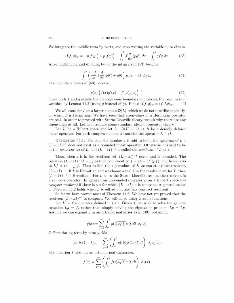
78 2. HILBERT SPACES
We integrate the middle term by parts, and stop writing the variable x, to obtain
〈Lf, g〉w = −p f ′g∣∣ba
+ p fg′∣∣ba−∫ b
a
fd
dx(pg′) dx−
∫ b
a
qfg dx. (53)
After multiplying and dividing by w, the integrals in (53) become∫ b
a
(−fw
(d
dx(pg′) + qg)
)wdx = 〈f, Lg〉w. (54)
The boundary terms in (53) become
p(x)(f(x)g′(x)− f ′(x)g(x)
) ∣∣ba. (55)
Since both f and g satisfy the homogeneous boundary conditions, the term in (55)vanishes by Lemma 11.2 (using g instead of g). Hence 〈Lf, g〉w = 〈f, Lg〉w.
We will consider L on a larger domain D(L), which we do not describe explicitly,on which L is Hermitian. We have seen that eigenvalues of a Hermitian operatorare real. In order to proceed with Sturm-Liouville theory, we ask why there are anyeigenvalues at all. Let us introduce some standard ideas in operator theory.
Let H be a Hilbert space and let L : D(L) ⊂ H → H be a densely definedlinear operator. For each complex number z consider the operator L− zI.
Definition 11.1. The complex number z is said to be in the spectrum of L if(L− zI)−1 does not exist as a bounded linear operator. Otherwise z is said to bein the resolvent set of L, and (L− zI)−1 is called the resolvent of L at z.
Thus, when z is in the resolvent set, (L − zI)−1 exists and is bounded. Theequation (L− zI)−1f = µf is then equivalent to f = (L− zI)(µf), and hence alsoto Lf = (z + 1
µ )f . Thus to find the eigenvalues of L we can study the resolvent
(L−zI)−1. If L is Hermitian and we choose a real k in the resolvent set for L, then(L − kI)−1 is Hermitian. For L as in the Sturm-Liouville set-up, the resolvent isa compact operator. In general, an unbounded operator L on a Hilbert space hascompact resolvent if there is a z for which (L− zI)−1 is compact. A generalizationof Theorem 11.2 holds when L is self-adjoint and has compact resolvent.
So far we have proved most of Theorem 11.2. We have not yet proved that theresolvent (L− kI)−1 is compact. We will do so using Green’s functions.
Let L be the operator defined in (50). Given f , we wish to solve the generalequation Lg = f , rather than simply solving the eigenvalue problem Ly = λy.Assume we can expand g in an orthonormal series as in (49), obtaining
g(x) =
∞∑j=1
∫ b
a
g(t)φj(t)w(t)dt φj(x).
Differentiating term by term yields
(Lg)(x) = f(x) =
∞∑j=1
(∫ b
a
g(t)φj(t)w(t)dt
)λjφj(x).
The function f also has an orthonormal expansion:
f(x) =
∞∑j=1
(∫ b
a
f(t)φj(t)w(t)dt
)φj(x).

11. STURM-LIOUVILLE THEORY 79
We equate coefficients to obtain
g(x) =
∫ b
a
∞∑j=1
φj(x)φj(t)
λjw(t)f(t) dt =
∫ b
a
G(x, t)f(t)w(t)dt. (56)
We summarize the story. Assume that a complete orthonormal system exists.Decompose the Hilbert space into eigenspaces Eλj . If h ∈ Eλj we have Lh = λjh.Note that no λj is zero. Thus, restricted to Eλj , we can invert L by
L−1(h) =1
λjh.
We invert L in general by inverting L on each eigenspace and adding up the results.Things are essentially the same as in Section 4 of Chapter 1, where we solved alinear system when there was an orthonormal basis of eigenvectors.
The kernel G is known as the Green’s function. In other words, if we know thatthere is an orthonormal basis of eigenfunctions, and 0 is not an eigenvalue, thenthis kernel is given by
G(x, t) =
∞∑j=1
φj(x)φj(t)
λj.
11.1. The Green’s function. In this subsection we construct the Green’sfunction G in another fashion, often used in Physics and Engineering. We willprove that the complete orthonormal system in the Sturm-Liouville setting exists.The construction is based on the following idea. Assume that 0 is not an eigenvaluefor L. Put G(x, t) = χt(x). Formally differentiating in x, we see that L(χ) = 0,except when x = t. We also see that χ must obey the boundary conditions (SL.1)and (SL.2). Finally, since Lg = f , we see that L(G)(x, t) behaves like a deltafunction when x = t. Thus we are led to defining G(x, t) as follows.
First we find a solution u to Lu = 0 that satisfies the boundary condition at a.Then we find a solution v of Lv = 0 that satisfies the boundary condition at b. PutG(x, t) = 1
cu(t)v(x) for t < x and G(x, t) = 1cu(x)v(t) for t > x. Then G extends
to be continuous when x = t. Thus Lu = 0 and Lv = 0, and hence, when x 6= t,L(χ) = 0. We put
c = p(x)W (x) = p(x)(u(x)v′(x)− u′(x)v(x)). (57)
By Lemma 11.3, c is a non-zero constant. Since L(v) = 0 we see that L(χ) = 0 fort < x. Since L(u) = 0 we see that L(χ) = 0 for t > x. Our choice of c guaranteesthat things work. The proof is a computation using the fundamental theorem ofcalculus. The following important theorem and its proof summarize our discussion.
Theorem 11.3. Consider the Sturm-Liouville equation (SL). Define L by (59)below. Let u be a solution to Lu = 0 satisfying boundary condition (SL.1) and va solution to Lv = 0 with boundary condition (SL.2). Define c by (57). Given fcontinuous, define y by
y(x) =1
c
∫ x
a
u(x)(vfw)(t)dt+1
c
∫ b
x
v(x)(ufw)(t)dt. (58)
Then y is twice differentiable and Ly = f .

80 2. HILBERT SPACES
Proof. We start with (58) and the formula (59) for L:
Ly =−pwy′′ − p′
wy′ − q
wy. (59)
We apply L to (58) using the fundamental theorem of calculus and compute. Thecollection of terms obtained where we differentiate past the integral must vanishbecause u, v satisfy Lu = Lv = 0. The remaining terms arise because of thefundamental theorem of calculus. The first time we differentiate we get
1
c(uvp)(x)− 1
c(uvp)(x) = 0.
The minus sign arises because the second integral goes from x to b, rather thanfrom b to x.
The next time we differentiate we obtain the termp
c(uxv − uvx)fw,
with all terms evaluated at x. The term in parentheses is minus the Wronskian. ByLemma 11.3, the entire expression simplifies to −(fw)(x). When we finally multiplyby −1
w in the definition of L, this expression becomes f(x). We conclude, as desired,that Ly = f . Since u, v are twice differentiable, p is continuously differentiable, andw, f are continuous, it follows that y is twice differentiable.
In order to finish the proof of the Sturm-Liouville theorem, we need to showonly that there is a real k such that (L − kI)−1 exists as a bounded, compactoperator. Assuming this point, we construct the Green’s function for L − kI inthe same fashion as when k = 0. Thus we can construct a continuous Green’soperator. We write (L − kI)−1f(x) =
∫ baf(t)G(x, t)dt. When G is continuous on
the rectangle [a, b]× [a, b], (L− kI)−1 is compact, by Proposition 10.4.Consider, for example, the simple special case where Ly = −y′′ on the interval
[0, 1] with boundary conditions y(0) = y(1) = 0. For each positive integer m, there
is an eigenvalue π2m2, corresponding to the normalized eigenfunction√
2sin(mπx).The kernel G(x, t) has the following expression
G(x, t) = 2
∞∑m=1
sin(mπx) sin(mπt)
π2m2.
One can also verify here that
G(x, t) =
x(1− t) x < tt(1− x) x > t
(60)
by differentiating twice the relation
y(x) = (1− x)
∫ x
0
tf(t) dt+ x
∫ 1
x
(1− t)f(t) dt.
Of course, we discover this formula by the prescription from Theorem 11.3. Thefunction x is the solution vanishing at 0. The function 1−x is the solution vanishingat 1. See Figure 5.
Exercise 11.1. Assume 0 ≤ x < 12 . Put L = −( d
dx )2 on [0, 1] with boundaryconditions y(0) = y(1) = 0. Equate the two expressions for the Green’s function to

11. STURM-LIOUVILLE THEORY 81
x(1-t) t(1-x)
G(x,t)
Figure 5. Green’s function for the second derivative
establish the identity
x =4
π2
∞∑r=0
(−1)rsin((2r + 1)πx)
(2r + 1)2.
Prove that this identity remains true at x = 12 .
Exercise 11.2. Consider the equation y′′ + λy = 0 with boundary conditionsy(0) − y(1) = 0 and y′(0) + y′(1) = 0. Show that every λ is an eigenvalue. Whydoesn’t this example contradict Theorem 11.2? Hint: Look carefully at (SL.1) and(SL.2).
Exercise 11.3. Suppose L ∈ L(H) is Hermitian. Find limn→∞ ||Ln||1n . Sug-
gestion: If L = L∗, then ||L2|| = ||L||2.
Exercise 11.4. Put the Bessel equation x2y′′ + xy′ + (λ2x2 − ν2)y = 0 intoSturm-Liouville form.
11.2. Exercises on Legendre polynomials. The next several exercises in-volve the Legendre polynomials. These polynomials arise throughout pure andapplied mathematics. We will return to them in Section 13.
We first remind the reader of a method for finding solutions to linear ordinarydifferential equations, called reduction of order. Consider a linear differential op-erator L of order m. Suppose we know one solution f to Ly = g. We then seeka solution of the form y = uf for some unknown function u. The function u′ willthen satisfy a homogeneous linear differential equation of order m− 1. We used a
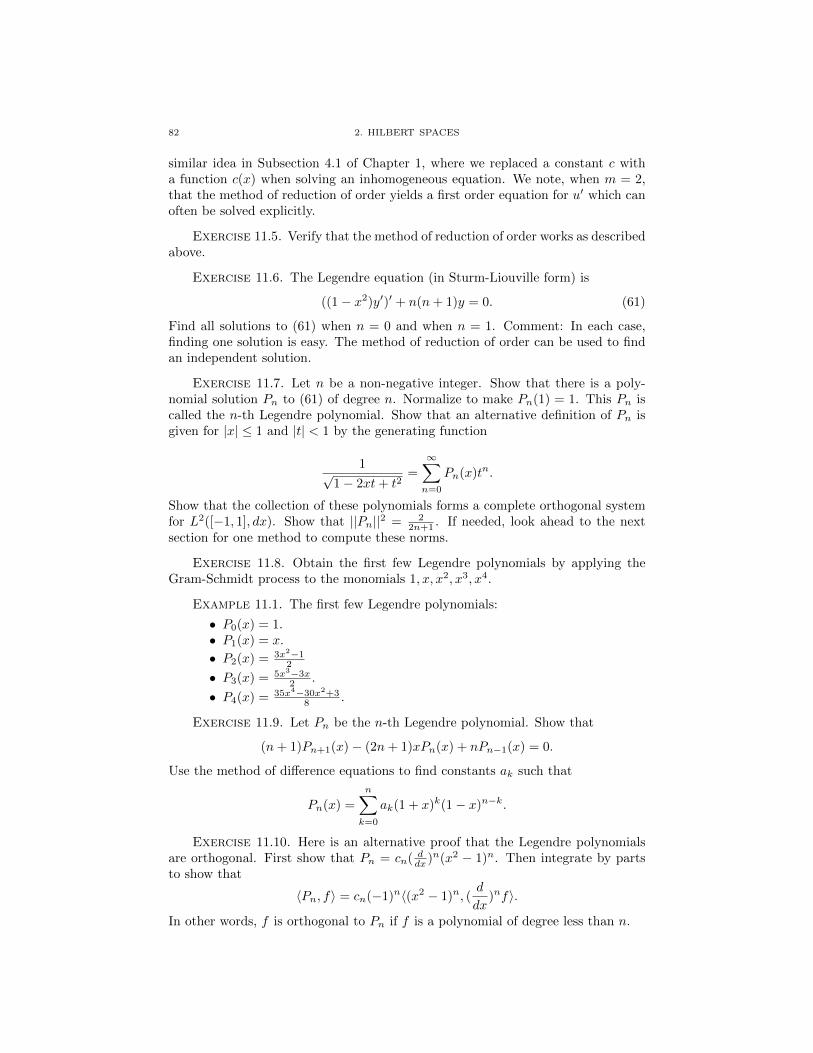
82 2. HILBERT SPACES
similar idea in Subsection 4.1 of Chapter 1, where we replaced a constant c witha function c(x) when solving an inhomogeneous equation. We note, when m = 2,that the method of reduction of order yields a first order equation for u′ which canoften be solved explicitly.
Exercise 11.5. Verify that the method of reduction of order works as describedabove.
Exercise 11.6. The Legendre equation (in Sturm-Liouville form) is
((1− x2)y′)′ + n(n+ 1)y = 0. (61)
Find all solutions to (61) when n = 0 and when n = 1. Comment: In each case,finding one solution is easy. The method of reduction of order can be used to findan independent solution.
Exercise 11.7. Let n be a non-negative integer. Show that there is a poly-nomial solution Pn to (61) of degree n. Normalize to make Pn(1) = 1. This Pn iscalled the n-th Legendre polynomial. Show that an alternative definition of Pn isgiven for |x| ≤ 1 and |t| < 1 by the generating function
1√1− 2xt+ t2
=
∞∑n=0
Pn(x)tn.
Show that the collection of these polynomials forms a complete orthogonal systemfor L2([−1, 1], dx). Show that ||Pn||2 = 2
2n+1 . If needed, look ahead to the nextsection for one method to compute these norms.
Exercise 11.8. Obtain the first few Legendre polynomials by applying theGram-Schmidt process to the monomials 1, x, x2, x3, x4.
Example 11.1. The first few Legendre polynomials:
• P0(x) = 1.• P1(x) = x.
• P2(x) = 3x2−12
• P3(x) = 5x3−3x2 .
• P4(x) = 35x4−30x2+38 .
Exercise 11.9. Let Pn be the n-th Legendre polynomial. Show that
(n+ 1)Pn+1(x)− (2n+ 1)xPn(x) + nPn−1(x) = 0.
Use the method of difference equations to find constants ak such that
Pn(x) =
n∑k=0
ak(1 + x)k(1− x)n−k.
Exercise 11.10. Here is an alternative proof that the Legendre polynomialsare orthogonal. First show that Pn = cn( d
dx )n(x2 − 1)n. Then integrate by partsto show that
〈Pn, f〉 = cn(−1)n〈(x2 − 1)n, (d
dx)nf〉.
In other words, f is orthogonal to Pn if f is a polynomial of degree less than n.
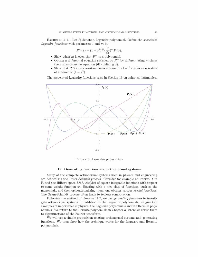
12. GENERATING FUNCTIONS AND ORTHONORMAL SYSTEMS 83
Exercise 11.11. Let Pl denote a Legendre polynomial. Define the associatedLegendre functions with parameters l and m by
Pml (x) = (1− x2)m2 (
d
dx)mPl(x).
• Show when m is even that Pml is a polynomial.• Obtain a differential equation satisfied by Pml by differentiating m-times
the Sturm-Liouville equation (61) defining Pl.• Show that Pml (x) is a constant times a power of (1−x2) times a derivative
of a power of (1− x2).
The associated Legendre functions arise in Section 13 on spherical harmonics.
P0 HxL
P1HxL
P2 HxL P3 HxL P4 HxL P5 HxL
-1.0 -0.5 0.5 1.0
-1.0
-0.5
0.5
1.0
Figure 6. Legendre polynomials
12. Generating functions and orthonormal systems
Many of the complete orthonormal systems used in physics and engineeringare defined via the Gram-Schmidt process. Consider for example an interval I inR and the Hilbert space L2(I, w(x)dx) of square integrable functions with respectto some weight function w. Starting with a nice class of functions, such as themonomials, and then orthonormalizing them, one obtains various special functions.The Gram-Schmidt process often leads to tedious computation.
Following the method of Exercise 11.7, we use generating functions to investi-gate orthonormal systems. In addition to the Legendre polynomials, we give twoexamples of importance in physics, the Laguerre polynomials and the Hermite poly-nomials. We return to the Hermite polynomials in Chapter 3, where we relate themto eigenfunctions of the Fourier transform.
We will use a simple proposition relating orthonormal systems and generatingfunctions. We then show how the technique works for the Laguerre and Hermitepolynomials.

84 2. HILBERT SPACES
Before stating and proving this proposition, we discuss vector-valued convergentpower series. Let B denote the open unit disk in C. Let H be a Hilbert space; itis often useful to consider complex analytic functions f : B→ H.
Consider a power series A(z) =∑Anz
n, where the coefficients An lie in H.This series converges at the complex number z if its partial sums there form aCauchy sequence in H. We define a function A : B→ H to be complex analytic ifthere is a sequence An in H such that the series
∞∑n=0
Anzn
converges to A(z) for all z in B. On compact subsets of B, the series converges innorm, and we may therefore rearrange the order of summation at will.
Proposition 12.1. Let H be a Hilbert space, and suppose A : B → H iscomplex analytic with A(t) =
∑∞n=0Ant
n. Then the collection of vectors Anforms an orthonormal system in H if and only if, for all t ∈ B,
||A(t)||2 =1
1− |t|2.
Proof. Using the absolute convergence on compact subsets to order the sum-mation as we wish, we obtain
||A(t)||2 =
∞∑m,n=0
〈An, Am〉tntm. (62)
Comparison with the geometric series yields the result: the right-hand side of (62)equals 1
1−|t|2 if and only if 〈An, Am〉 equals 0 for n 6= m and equals 1 for n = m.
Definition 12.1. The formal series
∞∑n=0
Lntn
is the ordinary generating function for the sequence Ln. The formal series
∞∑n=0
Lntn
n!
is the exponential generating function for the sequence Ln.
Explicit formulas for these generating functions often provide powerful insightas well as simple proofs of orthogonality relations.
Example 12.1 (Laguerre polynomials). Let H = L2 ([0,∞), e−xdx) be theHilbert space of square integrable functions on [0,∞) with respect to the measuree−xdx. Consider functions Ln defined via their generating function by
A(x, t) =
∞∑n=0
Ln(x)tn = (1− t)−1 exp
(−xt1− t
).

12. GENERATING FUNCTIONS AND ORTHONORMAL SYSTEMS 85
Note that x ≥ 0 and |t| < 1. In order to study the inner products 〈Ln, Lm〉,we compute ||A(x, t)||2. We will find an explicit formula for this squared norm;Proposition 12.1 implies that the Ln form an orthonormal system.
We have
|A(x, t)|2 = (1− t)−1 exp
(−xt1− t
)(1− t)−1 exp
(−xt1− t
).
Multiplying by the weight function e−x and integrating we obtain
||A(x, t)||2 = (1− t)−1(1− t)−1
∫ ∞0
exp
(−x(1 +
t
1− t+
t
1− t)
)dx.
Computing the integral on the right-hand side and simplifying shows that
||A(x, t)||2 =1
(1− t)(1− t)1
1 + t1−t + t
1−t
=1
1− |t|2.
From Proposition 12.1 we see that Ln forms an orthonormal system in H.The series defining the generating function converges for |t| < 1, and each Ln
is real-valued. In Exercise 12.2 we ask the reader to show that the functions Lnsatisfy the Rodrigues formula
Ln(x) =ex
n!
(d
dx
)n(xne−x) (63)
and hence are polynomials of degree n. They are called the Laguerre polynomials,and they form a complete orthonormal system for L2([0,∞), e−xdx). Laguerrepolynomials arise in solving the Schrodinger equation for a hydrogen atom.
A similar technique works for the Hermite polynomials, which arise in manyproblems in physics, such as the simple harmonic oscillator. We discuss thesepolynomials at the end of Chapter 3. One way to define the Hermite polynomialsis via the exponential generating function
exp(2xt− t2) =∑
Hn(x)tn
n!. (64)
The functionsHn are polynomials and form an orthogonal set forH = L2(R, e−x2
dx).With this normalization the norms are not equal to unity. In Exercise 12.4 thereader is asked to study the Hermite polynomials by mimicking the computationsfor the Laguerre polynomials. The reader should be aware that other normalizationsof these polynomials are also common. For example, sometimes the weight function
used is e−x22 . The advantage of this normalization is Theorem 9.1 of Chapter 3.
The technique of generating functions can also be used to find normalizingcoefficients. Suppose, such as in the Sturm-Liouville setting, that the collectionfn for n ≥ 0 forms a complete orthogonal system. We wish to find ||fn||L2 .Assume that we have found the generating function
B(x, t) =
∞∑n=0
fn(x)tn
explicitly. We may assume t is real. Taking L2 norms (in x) we discover that ||fn||2must be the coefficient of t2n in the series expansion of ||B(x, t)||2L2 .
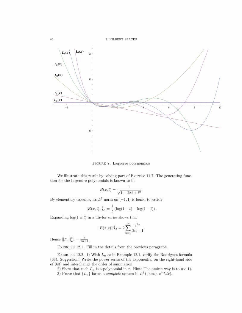
86 2. HILBERT SPACES
L0 HxL
L1HxL
L2 HxL
L3 HxL
L4 HxL L5 HxL
-2 2 4 6 8 10
-10
10
20
Figure 7. Laguerre polynomials
We illustrate this result by solving part of Exercise 11.7. The generating func-tion for the Legendre polynomials is known to be
B(x, t) =1√
1− 2xt+ t2.
By elementary calculus, its L2 norm on [−1, 1] is found to satisfy
||B(x, t)||2L2 =1
t(log(1 + t)− log(1− t)) .
Expanding log(1± t) in a Taylor series shows that
||B(x, t)||2L2 = 2
∞∑n=0
t2n
2n+ 1.
Hence ||Pn||2L2 = 22n+1 .
Exercise 12.1. Fill in the details from the previous paragraph.
Exercise 12.2. 1) With Ln as in Example 12.1, verify the Rodrigues formula(63). Suggestion: Write the power series of the exponential on the right-hand sideof (63) and interchange the order of summation.
2) Show that each Ln is a polynomial in x. Hint: The easiest way is to use 1).3) Prove that Ln forms a complete system in L2 ([0,∞) , e−xdx).
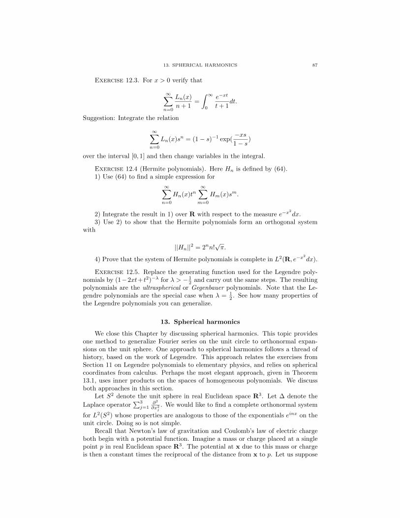
13. SPHERICAL HARMONICS 87
Exercise 12.3. For x > 0 verify that
∞∑n=0
Ln(x)
n+ 1=
∫ ∞0
e−xt
t+ 1dt.
Suggestion: Integrate the relation
∞∑n=0
Ln(x)sn = (1− s)−1 exp(−xs1− s
)
over the interval [0, 1] and then change variables in the integral.
Exercise 12.4 (Hermite polynomials). Here Hn is defined by (64).1) Use (64) to find a simple expression for
∞∑n=0
Hn(x)tn∞∑m=0
Hm(x)sm.
2) Integrate the result in 1) over R with respect to the measure e−x2
dx.3) Use 2) to show that the Hermite polynomials form an orthogonal system
with
||Hn||2 = 2nn!√π.
4) Prove that the system of Hermite polynomials is complete in L2(R, e−x2
dx).
Exercise 12.5. Replace the generating function used for the Legendre poly-nomials by (1−2xt+ t2)−λ for λ > − 1
2 and carry out the same steps. The resultingpolynomials are the ultraspherical or Gegenbauer polynomials. Note that the Le-gendre polynomials are the special case when λ = 1
2 . See how many properties ofthe Legendre polynomials you can generalize.
13. Spherical harmonics
We close this Chapter by discussing spherical harmonics. This topic providesone method to generalize Fourier series on the unit circle to orthonormal expan-sions on the unit sphere. One approach to spherical harmonics follows a thread ofhistory, based on the work of Legendre. This approach relates the exercises fromSection 11 on Legendre polynomials to elementary physics, and relies on sphericalcoordinates from calculus. Perhaps the most elegant approach, given in Theorem13.1, uses inner products on the spaces of homogeneous polynomials. We discussboth approaches in this section.
Let S2 denote the unit sphere in real Euclidean space R3. Let ∆ denote the
Laplace operator∑3j=1
∂2
∂x2j. We would like to find a complete orthonormal system
for L2(S2) whose properties are analogous to those of the exponentials einx on theunit circle. Doing so is not simple.
Recall that Newton’s law of gravitation and Coulomb’s law of electric chargeboth begin with a potential function. Imagine a mass or charge placed at a singlepoint p in real Euclidean space R3. The potential at x due to this mass or chargeis then a constant times the reciprocal of the distance from x to p. Let us suppose
88 2. HILBERT SPACES
that the mass or charge is located at the point (0, 0, 1). The potential at the pointx = (x1, x2, x3) is then
c
||x− p||=
c√(x2
1 + x22 + (x3 − 1)2)
. (65)
X
P
Φ
Figure 8. The co-latitude φ
We wish to express (65) in spherical coordinates. We write
x = (x1, x2, x3) = (ρcos(θ)sin(φ), ρsin(θ)sin(φ), ρcos(φ))
where ρ is the distance to the origin, θ is the usual polar coordinate angle in the(x1, x2) plane measuring longitude, and φ is the co-latitude. Thus 0 ≤ θ ≤ 2πwhereas 0 ≤ φ ≤ π. These conventions are common in calculus books, but thephysics literature often interchanges θ and φ. Also, sometimes r is used instead ofρ. In many sources, however, r is reserved for its role in cylindrical coordinates,and thus r2 = x2 + y2.
Writing (65) in spherical coordinates we obtain
c
||x− p||=
c√1 + ρ2 − 2ρcos(φ)
. (66)
The denominator in (66) is the same expression as in the generating function for theLegendre polynomials Pn from Exercise 11.7, with t replaced by ρ and x replacedby cos(φ). Therefore we can rewrite (66) as follows:
c
||x− p||= c
∞∑n=0
Pn(cos(φ))||x||n. (67)
The potential function from above is harmonic away from p. We leave thecomputation to the reader in Exercise 13.1. We write the Laplace operator inspherical coordinates:
∆(f) =1
ρ2
∂
∂ρ(ρ2fρ) +
1
ρ2sin(φ)
∂
∂φ(sin(φ)fφ) +
1
ρ2sin2(φ)fθθ. (68)
We attempt to solve the Laplace equation ∆(f) = 0 using separation of vari-ables, generalizing Exercise 11.7 of Chapter 1. Thus we assume that
f(ρ, θ, φ) = A(ρ)B(φ)C(θ). (69)

13. SPHERICAL HARMONICS 89
Plugging (69) into the Laplace equation yields the equation
0 = (ρ2A′BC)ρ +1
sin(φ)(sin(φ)AB′C)φ +
1
sin2(φ)ABC ′′. (70)
After dividing by ABC, we obtain
0 = (ρ2A′′ + 2ρA′
A) +
B′′
B+ cot(φ)
B′
B+
1
sin2(φ)
C ′′
C. (71)
The first fraction in (71) depends on ρ; the other terms do not. Hence there is aconstant λ such that
ρ2A′′ + 2ρA′ = λA. (72)
Furthermore we also have(B′′
B+ cot(φ)
B′
B
)sin2(φ) +
C ′′
C= −λsin2(φ). (73)
The only solutions to the equation (72) for A that are continuous at zero areA(ρ) = cρl for non-negative integers l. It follows that λ = l(l + 1).
Now we look at equation (73). Again by grouping the θ and φ terms separatelywe obtain two equations:
C ′′
C= −µ (74)
sin2(φ)
(B′′
B+ cot(φ)
B′
B+ λ
)= µ. (75)
Now (74) must be periodic in θ. Hence µ is the square of an integer k. We seethat C(θ) = ceikθ. Also (75) becomes
sin2(φ)
(B′′
B+ cot(φ)
B′
B+ λ
)= k2. (76)
Simplifying (76) leads to the equation
B′′ + cot(φ)B′ + (l(l + 1)− k2
sin2(φ))B = 0. (77)
Equation (77) evokes the differential equation defining the Legendre polynomials.In fact, if we make the substitution x = cos(φ), then (77) is precisely equivalent(See Exercise 13.3) to the equation
(1− x2)Bxx − 2xBx +
(l(l + 1)− k2
(1− x2)
)B = 0. (78)
The solutions P kl to (78) are the associated Legendre functions from Exercise11.11 when k ≥ 0 and related expressions for k < 0. The function eikθP kl (cos(φ))is the spherical harmonic Y kl (θ, φ). The integer parameter k varies from −l to l,yielding 2l+1 independent functions. The functions ρleikθP kl (cos(φ)) are harmonic.The functions Y kl are not themselves harmonic in general; on the sphere each Y klis an eigenfunction of the Laplacian with eigenvalue −l(l + 1).
A Wikipedia page called Table of spherical harmonics lists these Y kl , includingthe normalizing constants, for 0 ≤ l ≤ 10 and all corresponding k . The functionsY kl and Y ab are orthogonal, on L2(S2), unless k = a and l = b. These functionsform a complete orthogonal system for L2(S2). Remarkable additional propertieswhose discussion is beyond the scope of this book hold as well.

90 2. HILBERT SPACES
We next approach spherical harmonics via homogeneous polynomials. Thingsare simpler this way, but perhaps less useful in applied mathematics.
Let us write x, y, z for the variables. A polynomial p(x, y, z) is homogeneousof degree k if p(tx, ty, tz) = tkp(x, y, z). Homogeneous polynomials are thereforedetermined by their values on the unit sphere. For each n, we write Hn for thevector space of homogeneous harmonic polynomials of degree n. The dimension ofHn turns out to be 2n+ 1; see Theorem 13.1. We restrict these polynomials to theunit sphere to obtain spherical harmonics.
When n = 1, the harmonic polynomials x, y, z form a basis for H1. For n = 2,the following five polynomials form a basis for H2:
• xy• xz• yz• x2 + y2 − 2z2
• x2 − 2y2 + z2.
Note that the harmonic polynomial −2x2 + y2 + z2 is linearly dependent on thelast two items in the list.
Let Vn denote the vector space of homogeneous polynomials of degree n in thevariables x, y, z. We regard Hn as a subspace of Vn. The dimension of Vn is thebinomial coefficient
(n+2
2
). We have a map M : Vn → Vn+2 given by multiplication
by x2 +y2 +z2. The Laplace operator ∆ maps the other direction. These operatorsturn out to be adjoints. See Theorem 13.1.
We begin by defining inner products on the spaces Vn. We decree that thesespaces are orthogonal for distinct n. By linearity, to define the inner product onVn it suffices to define the inner product of monomials. We put
〈xaybzc, xAyBzC〉Vn = 0 (79)
unless a = A, b = B, and c = C. In this case we define ||xaybzc||2Vn = a!b!c!. Thusdistinct monomials are decreed to be orthogonal.
Theorem 13.1. The map M : Vn → Vn+2 is the adjoint of the map ∆ : Vn+2 →Vn. In other words,
〈Mf, g〉Vn+2= 〈f,∆g〉Vn . (80)
As consequences, the image of M is orthogonal to the harmonic space Hn+2 andVn+2 = M(Vn)⊕Hn+2. Furthermore Hn is of dimension 2n+ 1.
Proof. By linearity, it suffices to check (80) on monomials f = xaybzc andg = xAyBzC , where it follows by computing both sides of (80) in terms of factorials.There are three possible circumstances in which the inner product is not zero:
• (a, b, c) = (A− 2, B,C)• (a, b, c) = (A,B − 2, C)• (a, b, c) = (A,B,C − 2).
In the first case, we must check that (a + 2)!b!c! = A(A − 1)(A − 2)!B!C!, whichholds. The other two cases are similarly easy, and hence (80) holds.
Next, suppose that h is in the image of M and that g is in the nullspace of ∆.Then (80) gives
〈h, g〉Vn+2= 〈Mf, g〉Vn+2
= 〈f,∆g〉Vn = 0.

13. SPHERICAL HARMONICS 91
The desired orthogonality thus holds. The direct sum decomposition is immediate.
Finally, the dimension of Vn is (n+2)(n+1)2 . Since M is injective, the dimension of
the image of M is the dimension of Vn. The dimension of Hn+2 is therefore
(n+ 4)(n+ 3)
2− (n+ 2)(n+ 1)
2= 2n+ 5.
Hence the dimension of Hn is 2n+ 1.
Corollary 13.1. On the sphere we have Vn = Hn ⊕Hn−2 ⊕ . . . .
Proof. The formula follows by iterating the equality Vn = M(Vn−2)⊕Hn andnoting that x2 + y2 + z2 = 1 on the sphere.
Corollary 13.2. Suppose f is continuous on the unit sphere. Then there isa sequence of harmonic polynomials converging uniformly to f .
Proof. This proof assumes the Stone-Weierstrass theorem to the effect thata continuous function on a compact subset S of Rn is the uniform limit on S ofa sequence of polynomials. We proved this result in Corollary 10.2 of Chapter 1when S is the circle. Given this theorem, the result follows because, by the firstcorollary, each polynomial can be decomposed on the sphere in terms of harmonicpolynomials.
Corollary 13.3. The spherical harmonics form a complete orthogonal systemfor L2(S2).
We illustrate Corollary 13.1 for n = 0 and n = 1. Of course V0 is the span of theconstant 1. Its image underM is the span of x2+y2+z2. The spaceH2 is spanned bythe five functions xy, xz, yz, x2+y2−2z2, x2−2y2+z2. Each of these is orthogonal tox2 +y2 +z2, which spans the orthogonal complement of H2. Next, V1 is spanned byx, y, z. Its image underM is the span of x(x2+y2+z2), y(x2+y2+z2), z(x2+y2+z2).The space V3 has dimension ten. The seven-dimensional space H3 is the orthogonalcomplement of the span of M(V1).
Exercise 13.1. Show that (65) defines a harmonic function away from p. Useboth Euclidean coordinates and spherical coordinates.
Exercise 13.2. Verify formula (68).
Exercise 13.3. Use the chain rule (and some computation) to show that (77)and (78) are equivalent. Suggestion: First show that
Bφφ = Bxxx2φ +Bxxφφ.
Exercise 13.4. Express the harmonic polynomials of degree two using spher-ical coordinates.
Exercise 13.5. Find seven linearly independent harmonic polynomials of de-gree three.
Exercise 13.6. (Difficult) Analyze (78) fully in terms of Legendre polynomials.


CHAPTER 3
Fourier transform on R
1. Introduction
We define and study the Fourier transform in this chapter. Rather than workingwith functions defined on the circle, we consider functions defined on the real lineR. Among many books, the reader can consult [E], [G], and [GS] for applicationsof Fourier transforms to applied mathematics, physics, and engineering. See [F1]for an advanced mathematical treatment.
When |f | is integrable, we will define its Fourier transform by
F(f)(ξ) = f(ξ) =1√2π
∫ ∞−∞
f(x)e−ixξdx. (1)
In (1), the variable ξ is real. Thus f will be another function defined on the realline. We will then extend the definition of the Fourier transform by using methodsof functional analysis.
Along the way we will develop a deeper understanding of approximate identitiesand the Dirac delta function. We will define distributions or generalized functionsand thereby place the Dirac function on firm theoretical ground. For nice f wehave the Fourier inversion formula
f(x) =1√2π
∫ ∞−∞
f(ξ)eixξdξ. (2)
Our abstract approach leads to a definition of f for f ∈ L2(R) or even when itis a distribution. We prove the fundamental result (Plancherel theorem) that theFourier transform is unitary on L2(R) and hence
||f ||2L2 = ||f ||2L2 . (3)
We combine the Plancherel theorem and the Cauchy-Schwarz inequality toestablish the famous inequality which yields the Heisenberg uncertainty principlefrom quantum mechanics. We include a brief introduction to pseudo-differentialoperators which includes the Sobolev lemma in one dimension. We close this chapterwith a section on inequalities.
For functions defined on the circle, we observed that the more differentiablethe function, the faster its Fourier coefficients decay at infinity. An analogousphenomenon happens for functions on R. It therefore makes sense to begin ourstudy of the Fourier transform by restricting to smooth functions of rapid decay atinfinity.
93

94 3. FOURIER TRANSFORM ON R
2. The Schwartz space
The Schwartz space S consists of the smooth functions of rapid decay at infin-ity. This space is named for Laurent Schwartz, a different person from HermannSchwarz, whose name is associated with the Cauchy-Schwarz inequality. Here isthe precise definition:
Definition 2.1. The Schwartz space S consists of those infinitely differentiablecomplex-valued functions f on R such that, for all non-negative integers a, b,
lim|x|→∞
|x|a(d
dx)bf(x) = 0.
Functions in the Schwartz space decay so rapidly at infinity that, even after dif-ferentiating or multiplying by x an arbitrary (finite) number of times, the resulting
functions still decay at infinity. For any ε > 0, the Gaussian e−εx2
is in S. Smoothfunctions of compact support provide additional examples. For convenience werecall the existence of such functions.
Theorem 2.1. Let I denote any closed bounded interval on R and let J denoteany open interval containing I. Then there is an infinitely differentiable functionχ : R→ [0, 1] such that χ = 1 on I and χ = 0 off J .
I J
1
Figure 1. Cutoff Function
Proposition 2.1. The Schwartz space S is a complex vector space. It is closedunder differentiation and under multiplication by x.
Proof. Left to the reader.
We define the Fourier transform for f ∈ S as an integral:
F(f)(ξ) = f(ξ) =1√2π
∫ ∞−∞
f(x)e−ixξdx. (4)
The definition of S regards differentiation and multiplication on an equal foot-ing. Let D = d
dx denote differentiation and let M = Miξ denote multiplicationby iξ. Working on S is convenient for several reasons; in particular, the Fouriertransform exchanges these operations. Furthermore, as we will show in Theorem2.2, the Fourier transform maps S to itself bijectively. We can interpret the lasttwo items of the following Proposition as saying that F diagonalizes differentiation.
Proposition 2.2. The following elementary properties hold for Fourier trans-forms defined on S.
2. THE SCHWARTZ SPACE 95
(1) F is linear.
(2) ||f ||L∞ ≤ 1√2π||f ||L1 .
(3) f(ξ) = f(−ξ).
(4) Put fh(x) = f(x+ h). Then fh(ξ) = eihξ f(ξ).
(5) f ′(ξ) = iξf(ξ). That is, FD = MF .(6) D = F−1MF and M = FDF−1.
Proof. The first five items are left to the reader. The last item follows fromthe penultimate item and Theorem 2.2 below.
The reader should compare Proposition 2.2 with Lemma 9.1 of Chapter 1.
Proposition 2.3. The Fourier transform maps S to itself.
Proof. It follows by differentiating (4) under the integral sign (justified by
the rapid decay of f at infinity) that f is infinitely differentiable. Since FD = MFit follows for each positive integer k and integration by parts that
FDk = MkiξF .
All boundary terms vanish since we are working in S. It follows that f decays
rapidly if and only if f does. Hence F : S → S.
We next prove several lemmas which get used in establishing the fundamentalproperties of the Fourier transform. The proofs of Lemma 2.2 and Theorem 8.1 ofChapter 1 use the same basic idea.
Lemma 2.1. For f, g ∈ S we have∫ ∞−∞
f(x)g(x)dx =
∫ ∞−∞
f(ξ)g(ξ)dξ (5)
Proof. Because of the rapid decay of f and g, we can write either side of (5)as a double integral, and integrate in either order. Then each side of (5) equals thedouble integral
1√2π
∫ ∞−∞
∫ ∞−∞
f(x)g(ξ)e−ixξdxdξ.
Lemma 2.2. Assume f is differentiable on R and that f ′ is bounded. Let gsatisfy the following:
•∫∞−∞ g(y)dy = 1
•∫∞−∞ |y| |g(y)|dy <∞
Then
limε→0
∫ ∞−∞
f(x+ εy)g(y) dy = f(x). (6.1)
Proof. Since f is differentiable and f ′ is bounded, the mean-value theoremof calculus implies the following inequality:
|f(b)− f(a)| ≤ supt|f ′(t)| |b− a| = M |b− a|. (mvt)
Since g integrates to 1, we can write f(x) =∫∞−∞ f(x)g(y)dy. Using (mvt) we get

96 3. FOURIER TRANSFORM ON R
∣∣∣∣∫ ∞−∞
f(x+ εy)g(y) dy − f(x)
∣∣∣∣ =
∣∣∣∣∫ ∞−∞
(f(x+ εy)− f(x)) g(y) dy
∣∣∣∣≤M
∫ ∞−∞|εy||g(y)|dy. (6.2)
Since |yg(y)| is integrable, the expression in (6.2) is bounded by a constant timesε. The desired conclusion (6.1) then follows by the definition of a limit.
Remark 2.1. It is tempting to plug ε = 0 into (6.1). Doing so is not valid;the limit of an integral is not necessarily the integral of the limit. The reason isthat an integral is itself a limit, and one cannot in general interchange the order oflimits. See Exercise 2.8. This simple issue recurs throughout analysis; one needsappropriate hypotheses before one can interchange the order when taking limits.
Exercise 2.1. Prove that e−x2 ∈ S.
Exercise 2.2. Prove Propositions 2.1 and 2.2.
Exercise 2.3. Prove using complex variable theory that∫∞−∞ e−(x+iy)2dx is
independent of y and find its value.
Exercise 2.4. Compute the Fourier transform of e−a(x−µ)2 for a > 0 andµ ∈ R. (Use the previous exercise.) Comment: This result is of fundamentalimportance in probability theory. We use it in the proofs of Theorem 2.2 andTheorem 9.1.
Exercise 2.5. Compute the Fourier transform of 11+x2 using residues. Com-
ment: the answer depends on |ξ|.
Exercise 2.6. Compute the Fourier transform of χ, if χ(x) = 1 for |x| ≤ 1and χ(x) = 0 otherwise.
Exercise 2.7. Put g(η) = 1√2πe−|η|2
2 for η ∈ R. Show that g satisfies the
hypotheses of Lemma 2.2.
Exercise 2.8. Put f(x, y) = |x||y| for (x, y) 6= (0, 0). Show that
limx→0
limy→0
f(x, y) 6= limy→0
limx→0
f(x, y).
We have now understood the Schwartz space and developed some computa-tional facility with Fourier transforms. We are therefore in a position to prove theFourier inversion formula; this theorem is one of the most important results in pureand applied analysis. Nearly all the rest of this Chapter depends upon the inversionformula.
Theorem 2.2. F is a bijective map of S to itself. Furthermore, for f ∈ S, wehave the Fourier inversion formula
f(x) =1√2π
∫ ∞−∞
f(ξ)eixξdξ. (7)
3. THE DUAL SPACE 97
Proof. We use the Gaussian as an approximate identity. By Exercise 2.4,
the Gaussian e−x22 is its own Fourier transform. We exploit this fact (which uses
Exercise 2.3) as follows. We introduce the factor e−ε2ξ2
2 in the integrand on theright-hand side of (7). Then we compute
1√2π
∫f(ξ)eixξe
−ε2ξ22 dξ =
1
2π
∫ ∫f(y)e−i(
y−xε )εξe
−ε2ξ22 dydξ. (8)
Put µ = εξ and get
1
2π
∫ ∫f(y)e−i(
y−xε )µe
−|µ|22
1
εdµdy. (9)
We recognize the µ integral in (9) as the Fourier transform of the Gaussian G,
evaluated at y−xε . Use G = G to evaluate this integral. After making the change
of variables y−xε = η we see that the expression in (9) equals
1√2π
∫f(x+ εη)e
−|η|22 dη. (10)
We claim that the limit as ε tends to zero in (10) is f(x). The result follows fromLemma 2.2, after noting that
g(η) =1√2πe−|η|2
2
satisfies the hypotheses of the Lemma. See Exercise 2.7. Thus (7) holds.
The reader should note the extent to which the proof of Theorem 2.2 resemblesthe proofs of results from Chapter 1 such as Theorem 8.1.
The next exercise is a bit akin to opening Pandora’s box. Taking functions ofoperations such as differentiation is natural (see for example Section 6 of Chapter1) but somewhat hard to justify. Doing so without great care can lead to delicatelogical issues.
Exercise 2.9. Use the property D = F−1MF to give a plausible definition ofthe α-th derivative of a nice function, where 0 < α < 1. Check that Dα+β = DαDβ .More generally, try to define g(D) for various functions g. What technical difficultiesarise?
3. The dual space
The Schwartz space S is not a normed space, but we nonetheless require anotion of convergence. This notion is achieved via semi-norms. We define mea-surements of a function f as follows:
Definition 3.1. Let a, b be non-negative integers. We define ||f ||a,b by
||f ||a,b = sup
(|x|a
∣∣∣∣( ddx )bf(x)
∣∣∣∣) .These measurements are not norms because ||f ||a,b can be zero without f being
0. If ||f ||a,0 vanishes for some a, however, then f is the zero function. Note that wecould replace supremum by maximum in the definition of the semi-norm, because

98 3. FOURIER TRANSFORM ON R
functions in S are continuous and decay rapidly at infinity. The number of semi-norms is countable, and hence we can make S into a metric space. The distancebetween two functions is given by the formula
dist(f, g) =∑a,b
cab||f − g||a,b
1 + ||f − g||a,b,
where cab > 0 and is chosen to make the sum converge. For example, cab = 2−a−b isoften used. With this distance function, S is a complete metric space. See Exercise3.4. It is adequate to state the notion of convergence in terms of the semi-norms,rather than in an equivalent manner using this distance function.
Definition 3.2. A sequence fn converges to f in S if, for all a, b,
||fn − f ||a,b → 0.
Since S is a vector space, it would have sufficed to give the notion of convergenceto 0. To say that a sequence fn converges to 0 means that, any derivative of anypolynomial multiple of fn tends to 0 uniformly.
Definition 3.3. Let L : S → C be a linear functional. Then L is calledcontinuous if, whenever fn converges to f in S, then L(fn) converges to L(f) in C.
Definition 3.4. The dual space S ′ is the vector space consisting of all con-tinuous linear functionals on S. Elements of S ′ are called Schwartz distributions.
It is often convenient to write the action of a linear functional using innerproduct notation:
φ(f) = 〈f, φ〉.There is no complex conjugate used here.
Each element g of S can be regarded as a distribution by the formula
g(f) = 〈f, g〉 =
∫ ∞−∞
f(x)g(x)dx. (11)
The integral in (11) defines a distribution more generally. For example, when g isbounded and continuous, (11) makes sense and g can be regarded as an element ofS ′. When g is any function such that (11) makes sense for all f ∈ S, we regard g asthe element of S ′ defined by (11). Distributions are more general than functions.
Example 3.1 (Distributions). The most famous example of a distribution isthe Dirac delta function, henceforth called the Dirac delta distribution. We defineδ ∈ S ′ by
δ(f) = 〈f, δ〉 = f(0).
Another example is given by its derivative:
δ′(f) = 〈f, δ′〉 = 〈−f ′, δ〉 = −f ′(0).
More generally, if φ is a Schwartz distribution, we define its k-th derivative φ(k) by
φ(k)(f) = 〈f, φ(k)〉 = (−1)k〈f (k), φ〉. (12)

3. THE DUAL SPACE 99
By Exercise 3.1, (12) defines a continuous linear functional on S, and henceφ(k) ∈ S ′. Formula (12) is the natural definition of distribution derivative. If φ wereitself k times differentiable, then (12) would hold; we integrate by parts k timesand all boundary terms vanish.
Let us give another example of a distribution and its derivative. Define afunction u by u(x) = x for x ≥ 0 and u(x) = 0 for x < 0. This function issometimes called the ramp function. Then u′, which is not defined at 0 as a function,nonetheless defines a distribution. We have
u′(f) = −u(f ′) = −∫ ∞
0
x f ′(x) dx =
∫ ∞0
f(x) dx. (13)
In (13) the first equality is the definition of distribution derivative, the next equalityholds because u is a function, and the last equality holds via integration by parts.We also can compute the second derivative of u:
u′′(g) = −u′(g′) = −∫ ∞
0
g′(t) dt = g(0).
Thus u′′ = δ. The Dirac delta distribution is thus the second distribution derivativeof the ramp function u. The distribution H = u′ is known as the Heaviside function.It is named after Oliver Heaviside, rather than for the following reason. Note thatH = 1 on the positive axis and H = 0 on the negative axis. Thus H is “heavy” onthe right side. See [H] for a fascinating discussion of Heaviside’s life.
Exercise 3.1. Verify that δ ∈ S ′. If φ ∈ S ′, show that φ′, as defined by (12),also is in S ′.
If f is a continuous function, and φ is a distribution, then we naturally definef · φ by (f · φ)(g) = φ(fg). It is not possible to define the product of distributionsin general. See [SR] and its references for discussion of this issue.
Exercise 3.2. Let f be continuous and let δ be the Dirac delta distribution.Find the distribution derivative (f ·δ)′. Assuming f is differentiable, find f ′ ·δ+f ·δ′.
Definition 3.5 (The generalized Fourier transform). Let φ ∈ S ′. We defineits Fourier transform F(φ) by duality as follows. For each f ∈ S we decree that
〈F(φ), f〉 = 〈φ,F(f)〉.
The Fourier transform F(φ) is itself a distribution. It is obviously linear. We
verify continuity. If fn converges to 0 in S, then fn also converges to 0 in S. Hence〈φ,F(fn)〉 converges to 0 in C.
Example 3.2. What is the Fourier transform of the Dirac delta? We have
〈δ, f〉 = 〈δ, f〉 = f(0) =1√2π
∫ ∞−∞
f(x)dx = 〈 1√2π, f〉.
Thus δ is the constant function 1√2π
.
Exercise 3.3. Compute the Fourier transforms H and u.
Exercise 3.4. Fill in the discussion between Definition 3.1 and 3.2 as follows.Verify that the given alleged distance function is in fact a distance function. Thenuse the Arzela-Ascoli theorem to show that S is a complete metric space.
100 3. FOURIER TRANSFORM ON R
Exercise 3.5. Let φ be a linear functional on S. Show that φ ∈ S ′ if and onlyif there is a constant M and an integer N such that
|φ(f)| ≤Mmax||f ||a,b : a+ b ≤ N.
4. Convolutions
We have already observed the power of convolution in understanding Fourierseries. We extend the notion of convolution to R and obtain similarly powerfulresults.
Definition 4.1. Suppose f and g are integrable functions on R. We definef ∗ g by
(f ∗ g)(x) =
∫ ∞−∞
f(x− y)g(y)dy. (14)
We immediately observe by change of variables that f ∗ g = g ∗ f . We also caneasily check that if f ∈ L1 and g ∈ L2, then f ∗ g ∈ L2.
Theorem 4.1. If f and g are in L1, then (f ∗ g) =√
2πf g.
Proof. We write out (f ∗ g)(ξ) as a double integral and interchange the order
of integration, obtaining√
2πf g.
We wish to extend our work on approximate identities to this setting. First letχ denote any integrable smooth function such that
∫∞−∞ χ(x)dx = 1. For ε > 0 we
then define χε by
χε(x) =χ(xε )
ε. (15)
Then, by change of variables,∫∞−∞ χε(x)dx = 1 also.
Definition 4.2. For χε as in (15), put Jε(f) = χε ∗ f . We call Jε a mollifier.
Theorem 4.2. If f ∈ L1, then Jεf converges to f in L1 as ε tends to 0. Iff ∈ L2, then Jεf converges to f in L2 as ε tends to 0. If f is uniformly continuousnear x, then Jεf converges uniformly to f near x. If f is integrable and χ isinfinitely differentiable, then Jεf is infinitely differentiable.
Proof. We refer the reader to Chapter 8 of [F2].
Exercise 4.1. Show that the function f defined by f(x) = e−1x for x > 0 and
by f(x) = 0 otherwise is infinitely differentiable. Sketch the graph of the functionx→ f(x)f(1− x).
Exercise 4.2. Prove Theorem 2.1. Suggestion: First find a continuous func-tion that is 1 on I and 0 off J . Mollify it, using a function χ as constructed in theprevious exercise.
Exercise 4.3. The support of a function f is the smallest closed set outside ofwhich f is identically zero. Suppose f is supported in [a, b] and g is supported in[c, d]. What can you say about the support of f ∗ g?
5. PLANCHEREL THEOREM 101
5. Plancherel theorem
The Parseval formula equates the l2-norm of the Fourier coefficients of a func-tion with the L2 norm of the function. Its polarized form, Corollary 8.4 of Chapter2, states that
〈f , g〉2 = 〈f, g〉L2 .
The Plancherel theorem (which holds both in higher dimensions and in more ab-stract settings) extends the Parseval result by establishing that the Fourier trans-form is a unitary operator on L2(R).
Recall that the Fourier transform is defined on L2 in a subtle manner; theintegral in (1) need not converge for f ∈ L2. We define F on the Schwartz spacevia integration as in (1), and then we extend F to S ′ by duality. We then regard anelement of L2 as an element of S ′. It would also be possible to define F on L1 ∩L2
by the integral (1) and proceed by limiting arguments.
Theorem 5.1. The Fourier transform F : L2(R)→ L2(R) is unitary.
Proof. By Proposition 7.2 of Chapter 2 it suffices to check that ||Ff ||2L2 =||f ||2L2 for all f in L2. The norm is continuous, and hence it suffices to check this
equality on the dense set S. Put g = f in Lemma 2.1. Then g = f and Lemma 2.1
gives ||f ||2L2 = ||f ||2L2 .
Exercise 5.1. First note that F4 = I. Use this fact and Exercise 2.4 to findall eigenvalues of F . Harder: Find all eigenfunctions. Suggestion: Apply d
dx − x to
e−x22 and use formula (64) from Chapter 2.
Exercise 5.2. Put χ(x) = 1 for −1 ≤ x ≤ x and χ(x) = 0 otherwise. Find χ.
Exercise 5.3. Use Exercise 5.2 and the Plancherel Theorem to find∫∞−∞
sin2(x)x2 dx.
Also use contour integration to check your answer.
Exercise 5.4. Assume b ≥ 0. Compute the integrals:∫ ∞0
e−u(1+x2)du.
∫ ∞−∞
e−ibx
1 + x2dx.
∫ ∞0
e−t√te−b24t dt.
Suggestion: Use the first, the second, and the Fourier transform of a Gaussian tocompute the third. The answer to the third is
√π exp(−b).
Exercise 5.5. Put f(x) = e−xxa−1 for x ≥ 0 and f(x) = 0 otherwise. Find
the condition on a for which f ∈ L1(R). Under this condition, find f . Comment.One can use contour integrals from complex analysis here.

102 3. FOURIER TRANSFORM ON R
6. Heisenberg uncertainty principle
The famous Heisenberg uncertainty principle from quantum mechanics statessomething to the effect that it is not possible to determine precisely both the posi-tion and momentum of a moving particle. This principle can be formulated as aninequality involving the Fourier transform. After giving an intuitive explanation,we state and prove this inequality.
Let |f |2 denote the probability density on R determined by the position of amoving particle. By definition, the probability that this particle is found in the
interval [a, b] is the integral∫ ba|f(x)|2dx and of course
∫∞−∞ |f(x)|2dx = 1 (the
particle is somewhere).The mean (expected value) of position is by definition the integral
µ =
∫ ∞−∞
x|f(x)|2dx.
After a translation we may assume without loss of generality that µ = 0.
The picture for momentum looks the same, except that we use |f |2 to define
the density for momentum. By the Plancherel theorem, |f |2 also defines a density.Again, without loss of generality, we may assume (after multiplying f by a constantof modulus 1) that the mean of momentum is 0. See Exercise 6.1.
The variance of the position of a particle of mean 0 equals∫ ∞−∞
x2|f(x)|2dx = ||xf(x)||2L2 ,
and the variance of its momentum is∫ ∞−∞
ξ2|f(ξ)|2dξ = ||ξf(ξ)||2L2 .
The following famous inequality gives a positive lower bound on the productof the two variances.
Theorem 6.1 (Heisenberg uncertainty principle). Assume both f and f ′ aresquare-integrable on R. Then
||xf(x)||2L2 ||ξf(ξ)||2L2 ≥1
4||f ||4L2 . (16)
Proof. We assume that f ∈ S. The general case follows because S is densein L2. Consider the integral
I =
∫ ∞−∞
x(f(x)f
′(x) + f ′(x)f(x)
)dx.
Using integration by parts, we obtain
I = x|f(x)|2∣∣∞−∞ −
∫ ∞−∞|f(x)|2dx = −
∫ ∞−∞|f(x)|2dx,
because the boundary terms are zero. By the Cauchy-Schwarz inequality and thePlancherel theorem, we also have
|I| ≤ 2||xf(x)||L2 ||f ′||L2 = 2||xf(x)||L2 ||ξf(ξ)||L2 . (17)
Putting the two formulas together gives
1
2||f ||2L2 ≤ ||xf(x)||L2 ||ξf(ξ)||L2 , (18)

7. DIFFERENTIAL EQUATIONS 103
which yields (16) upon squaring both sides.
Corollary 6.1. The following inequality holds:
||f ||2L2 ≤ ||xf(x)||2L2 + ||ξf(ξ)||2L2 = ||xf(x)||2L2 + ||f ′(x)||2L2 .
Proof. For non-negative real numbers s, t we always have st ≤ s2+t2
2 . (Thearithmetic-geometric mean inequality, or the Cauchy-Schwarz inequality!). Ap-plying this simple fact to the product on the right-hand side of (18) yields theinequality. The equality follows by Proposition 2.2.
Exercise 6.1. What is the effect on the mean of position if we replace f(x)by eixhf(x)? What is the effect on the mean of momentum in doing so?
Exercise 6.2. When does equality hold in (16)?
A less precise form of the Heisenberg uncertainty formula says the following.
Unless f is identically 0, then f and f cannot both vanish outside of a boundedset. We prove this result next.
Theorem 6.2. Suppose f is integrable on [−r, r] and f(x) = 0 for |x| > r. If
there is an R such that f(ξ) = 0 for |ξ| > R, then f is identically 0.
Proof. We start with
f(ξ) =1√2π
∫ r
−rf(x)e−ixξdx. (19)
In (19) we regard ξ as a complex variable. Since we may differentiate under theintegral as often as we wish (introducing factors of −ix) and the integral still
converges, ξ → f(ξ) is an entire complex analytic function. If an R exists as inthe theorem, then this complex analytic function vanishes on an interval in R. Bybasic complex variable theory, a complex analytic function vanishing on an interval
of the real axis must be identically 0. Thus both f and f vanish identically.One can also prove the theorem as follows. Expand e−ixξ in a Taylor series
about any point and interchange the order of integration and summation. We see
that f is an entire analytic function with a zero of infinite order, and hence it isidentically 0.
7. Differential equations
The Fourier transform plays a major role in partial differential equations. Al-though most of this material is beyond the scope of this book, we can glimpse someof the ideas in simple settings. The key point is that the Fourier transformationdiagonalizes differentiation. When we have diagonalized an operation, we can takefunctions of the operation.
We first consider diagonalization is a simple but interesting context. Consideran affine function z 7→ mz + w = f(z) on C. We write f∗n for the iteration of f atotal of n times. Thus f∗1 = f and f∗(n+1) = f f∗n. Using diagonalization, wecan compute f∗n easily.
There are two cases. When f(z) = z + w (thus f is a translation), we obtainf∗n(z) = z + nw. When f(z) = mz + w for m 6= 1, we can write
f(z) = mz + w = m(z + ζ)− ζ,
104 3. FOURIER TRANSFORM ON R
where mζ − ζ = w. We see that f = T−1MT , where T is translation by ζ and Mis multiplication by m. Thus f∗n = T−1MnT , or
f∗n(z) = mn(z + ζ)− ζ.The simplicity of these formulas is evident. Furthermore, the formulas make
sense when n is replaced by an arbitrary real number α as long as we are carefulin our definition of the multi-valued function m → mα. The crucial point is thatwe can take functions of operators. Often we simply want to find f−1, but we cando more, such as raising f to an arbitrary power α.
This technique of diagonalization applies to differential equations via the Fouriertransform. The starting point is the inversion formula (3). When differentiatingunderneath the integral sign is valid, we obtain
f (k)(x) =1√2π
∫ ∞−∞
(iξ)kf(ξ)eixξdξ.
Thus the process of differentiating k times can be regarded as follows: first takethe Fourier transform. Then multiply by (iξ)k. Then take the inverse Fouriertransform. The reader should compare this process with the discussion in Section4 of Chapter 1 as well as with the above paragraphs.
Let p be a monic polynomial of degree k. Consider a linear differential equationof the form
p(D)y = y(k) −k−1∑j=1
cjy(j) = f. (20)
Taking Fourier transforms of both sides, we obtain a relation
(iξ)ky(ξ)−k−1∑j=1
cj(iξ)j y(ξ) = p(iξ)y(ξ) = f(ξ), (21)
which is an algebraic equation for y. Thus y(ξ) = f(ξ)p(iξ) for the polynomial p which
defines the differential equation. To solve (20), we take the Fourier transform of f ,divide by this polynomial in iξ, and recover y by finally taking the inverse Fouriertransform. The problem of integrating a differential equation gets replaced by theproblem of dividing by a polynomial and taking the inverse Fourier transform ofthe result.
Example 7.1. Consider y′′−y = f . We obtain y(ξ) = −f(ξ)1+ξ2 . Using the Fourier
inversion formula, we get
y(x) =−1
2π
∫ ∫f(t)
eiξ(x−t)
1 + ξ2dt dξ.
For nice f we can invert the order of integration and obtain a formula y(x) =∫G(x, t)f(t)dt.
Example 7.2. We return to the wave equation uxx = utt. Assume u(x, 0) =f(x) and ut(x, 0) = g(x). We apply the Fourier transform in x, regarding t asa parameter. The wave equation becomes a second order ODE with two initialconditions:
utt(ξ, t) = −ξ2u(ξ, t)
u(ξ, 0) = f(ξ)

8. PSEUDO-DIFFERENTIAL OPERATORS 105
ut(ξ, 0) = g(ξ).
Solving this second order ODE is easy, as it has constant coefficients when t isregarded as the variable. We get
u(ξ, t) = f(ξ)cos(|ξ|t) + g(ξ)sin(|ξ|t)|ξ|
. (22)
See Exercise 7.2 for the simple details.Now we can find u by applying the Fourier inversion formula.
Exercise 7.1. Suppose the f in Example 7.1 lies in the Schwartz space. FindG(x, t). Be careful about the sign of x− t.
Exercise 7.2. Fill in the details in Example 7.2.
Exercise 7.3. Let V be a complex vector space. Put f(z) = Mz + b, forM ∈ L(V, V ). Under what condition does f = T−1MT for some translation T?
8. Pseudo-differential operators
This section indicates how the Fourier transform has been used in modernanalysis. Let us repeat the idea from the previous section, by differentiating theFourier inversion formula for a Schwartz function u:
(d
dx)ku(x) =
1√2π
∫ ∞−∞
eixξ(iξ)ku(ξ)dξ. (23)
Let pk(x) be a smooth function of x and let (Lu)(x) =∑mk=0 pk(x)u(k)(x) denote
a differential operator of order m. By (23) we have
Lu(x) =
m∑k=0
pk(x)u(k)(x) =1√2π
∫ ∞−∞
eixξm∑k=0
(iξ)kpk(x)u(ξ)dξ.
As before, Lu is computed by a three-step process. We find u; we multiplyby a polynomial in ξ with coefficients in x, namely
∑k pk(x)(iξ)k; finally we take
the inverse Fourier transform. To invert L we proceed in a similar fashion, withmultiplication replaced by division.
A pseudo-differential operator P is a linear operator, defined on a space offunctions or distributions, obtained in the following fashion. Given u, we computePu as follows. We find u(ξ); we multiply by a smooth function p(x, ξ) satisfyingappropriate smoothness conditions in (x, ξ) and growth restrictions in ξ; finally wetake the inverse Fourier transform. The function p(x, ξ) is called the symbol of P .
One of the most useful examples is the pseudo-differential operator Λs. Itssymbol is (1 + ξ2)
s2 . The operator Λ2 is the same as 1− ( d
dx )2. Note that Λ−2 is its
inverse. Hence we can solve the differential equation (1 − ( ddx )2)u = f by writing
f = Λ−2u. The operator Λ−2 is certainly not a differential operator, although it isthe inverse of one.
Pseudo-differential operators extend this idea to both ordinary and partial lin-ear differential equations. The key idea is to perform algebraic operations (multi-plication and division) on the symbols, rather than to differentiate and integrate.
What functions are allowed as symbols? Perhaps the most basic class of sym-bols, but not the only one, is defined as follows. For m ∈ R, we let Sm denote the
106 3. FOURIER TRANSFORM ON R
space of infinitely differentiable functions u in (x, ξ) such that, for all a, b there isa constant Cab such that
∣∣( ddx
)a(d
dξ)bu(x, ξ)
∣∣ ≤ Cab(1 + ξ2)m−b
2 . (24)
Elements of Sm are called symbols of order m. A pseudo-differential operator hasorder m if its symbol has order m. In particular, a differential operator gives anexample of a pseudo-differential operator of the same order. For each real numbers, the operator Λs has order s.
We obviously have Sl ⊂ Sm if l ≤ m. We therefore naturally define S∞ = ∪Sm
and S−∞ = ∩Sm. The reader might wonder what an operator of order −∞ mightbe. Mollifiers as we defined earlier provide nice examples. These operators smooththings out, as we indicate below.
These ideas are part of a sophisticated theory including Sobolev spaces. See[SR] for example. For us the key point to mention extends our earlier remark tothe effect that the smoothness of a function on the circle is related to the rate ofdecay of its Fourier coefficients at ∞. Sobolev spaces measure the rate of decay at∞ of the Fourier transform of a function. We give the following definition of theSobolev space Hs(R). Henceforth we drop the R from the notation.
Definition 8.1. Assume u ∈ S ′. Then u ∈ Hs if and only if Λsu ∈ L2(R).
This definition is equivalent to demanding that u be a function for which
||u||2Hs =
∫ ∞−∞
(1 + ξ2)s|u(ξ)|2dξ <∞. (24)
Note that Hs ⊂ Ht if s ≥ t. We naturally put H−∞ = ∪sHs and H∞ = ∩sHs.We then have the obvious additional containments, each of which is strict:
S ⊂ H∞ ⊂ H−∞ ⊂ S ′.
Exercise 8.1. Show that 11+x2 is in H∞ but not in S.
Lemma 8.1. Suppose |g| is integrable on R. Then both the Fourier transformof g and the inverse Fourier transform of g are continuous.
Proof. See Exercise 8.2.
The significance of Lemma 8.1 arises from the following crucial idea. To provethat a function or distribution u has k continuous derivatives, we take Fouriertransforms and prove that ξku(ξ) is integrable. This method clarifies the relation-ship between smoothness of a function and the behavior of its Fourier transform atinfinity.
Exercise 8.2. Prove that the Fourier transform of an L1 function is continuous.Be careful in your proof, as the real line is not compact.
Theorem 8.1. Assume u ∈ L2(R) and let k be an integer or ∞. Then:
• u ∈ Hk if and only if u(k) ∈ L2(R).• (Sobolev lemma, special case) If u ∈ Hs for s > k + 1
2 , then u has kcontinuous derivatives.

9. HERMITE POLYNOMIALS 107
Proof. First we note two obvious estimates.
|ξ|2k ≤ (1 + |ξ|2)k ≤ 2k if |ξ| ≤ 1 (25.1)
|ξ|2k ≤ (1 + |ξ|2)k ≤ 2k|ξ|2k if 1 ≤ |ξ|. (25.2)
The inequalities in (25.1) and (25.2) show that u ∈ Hk is equivalent to u(k) beingsquare-integrable, and the first statement holds. To prove the second statement,we estimate using the Cauchy-Schwarz inequality:∫
|ξ|k|u(ξ)| =∫
|ξ|k
(1 + |ξ|2)s2|u(ξ)|(1 + |ξ|2)
s2 ≤ ||u||Hs
(∫|ξ|2k
(1 + |ξ|2)s
) 12
. (26)
The integral on the far right in (26) is convergent if and only if 2k − 2s < −1.Hence, if u ∈ Hs and s > k+ 1
2 , then the expression |ξ|ku(ξ) is integrable. Since werecover the k-th derivative of u by taking the inverse Fourier transform, the secondstatement now follows from Lemma 8.1.
Corollary 8.1. Suppose u ∈ S ′ and u(k) ∈ L2 for all k. Then u agrees withan infinitely differentiable function almost everywhere.
Exercise 8.3. For what s is the Dirac delta distribution in Hs?
Exercise 8.4. Consider the analogue of the integral in (26) in n dimensions:∫Rn
||ξ||2k
(1 + ||ξ||2)sdV.
What is the condition on k, s, n such that this integral converges?
9. Hermite polynomials
We saw in Chapter 2 that the Hermite polynomials Hn(x) have the exponentialgenerating function exp(2xt− t2). In other words,
exp(2xt− t2) =
∞∑n=0
Hn(x)tn
n!. (27)
These polynomials are closely related to the Fourier transform.
Theorem 9.1. For each non-negative integer n, the function e−x22 Hn(x) is an
eigenfunction of the Fourier transform with eigenvalue (−i)n.
Proof. We start with (27) and multiply both sides by e−x22 . We then take
Fourier transforms. Doing so yields
F(
exp(−x2
2+ 2xt− t2)
)(ξ) =
∑n
F(e−x22 Hn(x)
)(ξ)
tn
n!. (28)
We will simplify the left-hand side of (28) and use (27) again to obtain the result.Note that
exp(−x2
2+ 2xt− t2) = exp(
−1
2(x− 2t)2) exp(t2). (29)
Plugging (29) into (28) replaces the left-hand side with
exp(t2)F(
exp(−1
2(x− 2t)2)
)(ξ). (30)
108 3. FOURIER TRANSFORM ON R
The second factor in (30) is the Fourier transform of a Gaussian with mean 2t andvariance 1. By Exercise 2.4, the Fourier transform of the Gaussian with mean µand variance 1 is exp(−iµξ) times itself. The expression in (30) therefore becomes
exp(t2 − 2iξt) exp(−ξ2
2). (31)
The first factor in (31) is the left-hand side of (27) with t replaced by (−it) and xreplaced by ξ. Using the generating function expansion from (27) with t replacedby −it, and equating coefficients of tn, yields the conclusion:
F(
exp(−x2
2)Hn(x)
)(ξ) = (−i)n exp(
−ξ2
2)Hn(ξ).
Example 9.1. The first few Hermite polynomials:
• H0(x) = 1• H1(x) = 2x• H2(x) = −2 + 4x2
• H3(x) = −12x+ 8x3
• H4(x) = 12− 48x2 + 16x4
• H5(x) = 120x− 160x3 + 32x5
• H6(x) = −120 + 720x2 − 480x4 + 64x6
• H7(x) = −1680x+ 3360x3 − 1344x5 + 128x7.
Figure 2 shows the polynomials Hn(x)/2n for 0 ≤ n ≤ 5. We divide by 2n tomake the leading coefficient equal to 1, and the graphs become nicer.
Exercise 9.1. Write simple code to get Mathematica or something similar toprint out the first twenty Hermite polynomials. Observe some patterns and thenprove them.
Exercise 9.2. For each n find (x− ddx )n exp (−x
2
2 ).
Exercise 9.3. Prove that H ′n(x) = 2xHn(x)−Hn+1(x).
Exercise 9.4. Prove for each n that Hn(x) has integer coefficients.
Exercise 9.5. Let M denote multiplication by exp(−x2) and let T denotex− d
dx . Express M−1TnM in terms of Hermite polynomials.
Exercise 9.6. We saw in Chapter 2 that the Hermite polynomials form a com-plete orthogonal system for H = L2(R, exp(−x2)). Show that ||Hn||2 = 2nn!
√π.
Exercise 9.7. Find a combinatorial interpretation of the sequence of (absolutevalues of) coefficients 0, 0, 0, 2, 12, 48, 160, 480, . . . of the second highest power of xin Hn(x).
10. More on Sobolev spaces
We begin by proving the following theorem. Its proof is quite similar to severalproofs from Chapter 1. The analogues of this result and the subsequent propositionin higher dimensions are important tools in partial differential equations. See forexample [F1] and [Ra].
Theorem 10.1. Assume s < t. Let fn be a sequence of functions such that:

10. MORE ON SOBOLEV SPACES 109
-1.0 -0.5 0.5 1.0
-1.0
-0.5
0.5
1.0
Figure 2. Scaled Hermite polynomials
• There is a constant C such that ||fn||Ht ≤ C for all n.
• fn(ξ) converges uniformly to 0 on compact subsets of R.
Then ||fn||Hs converges to 0.
Proof. We start with
||fn||2Hs =
∫(1 + |ξ|2)s|fn(ξ)|2 dξ. (32)
As in many proofs in this book, we estimate the integral by breaking it into twoparts. First consider the set where |ξ| > R. On this set, and remembering thats < t, we have
(1 + |ξ|2)s = (1 + |ξ|2)s−t(1 + |ξ|2)t ≤ (1 +R2)s−t(1 + |ξ|2)t. (33)
Using (33) in (32) we obtain
||fn||2Hs ≤∫|ξ|≤R
(1 + |ξ|2)s|fn(ξ)|2 dξ + (1 +R2)s−t||fn||2Ht . (34)
Suppose ε > 0 is given. Since the terms ||fn||2Ht are bounded, and s < t, we maychoose R large enough to guarantee that the second term on the right-hand side of(34) is at most ε
2 . Fix this R. Now consider the first term on the right-hand side of
(34). It is bounded by a constant (independent of n) times sup|fn(ξ)|2. Since theset where |ξ| ≤ R is compact, the assumption of uniform convergence allows us tobound this term by ε
2 , by choosing n large enough.

110 3. FOURIER TRANSFORM ON R
Proposition 10.1. Suppose s < t < u and ε > 0. Then there is a constant Cεsuch that
||f ||2Ht ≤ ε||f ||2Hu + Cε||f ||2Hs . (35)
Proof. For any positive x we have 1 ≤ xu−t + xs−t since one of x and 1x is
already at least 1. Plug in (1 + |ξ|2)ε1u−t for x. We get
1 ≤ ε(1 + |ξ|2)u−t + εs−tu−t (1 + |ξ|2)u−t.
Then multiply this inequality by (1+ |ξ)|2)t|f(ξ)|2 and integrate. The result is that
||f ||2Ht ≤ ε||f ||2Hu + Cε||f ||2Hs ,
where Cε = εs−tu−t . Note that Cε is a negative power of ε.
One can also write this proof using the operators Λr where r = u − t andr = s− t. Equivalently, put g = Λtf in (35). We obtain an estimate of the L2 normof g in terms of a small constant times a Sobolev norm with a positive index and alarge constant times a Sobolev norm with negative index.
These results are closely related to the Rellich Lemma. See for example [F1].Often one considers Sobolev spaces Hs(Ω) on a bounded domain or compact mani-fold Ω. The Rellich Lemma then states that the inclusion map of Ht(Ω) into Hs(Ω)is a compact operator when s < t. If we work with Sobolev spaces on R, we maystate the Rellich Lemma as follows:
Theorem 10.2 (Rellich lemma). Assume that gn is a bounded sequence inHt and each gn vanishes outside a fixed compact set K. Then, whenever s < t,there is a subsequence gnk converging in Hs.
The proof is similar to that of Theorem 10.1. Under the hypotheses of theRellich lemma, and using the Arzela-Ascoli theorem, one can find a subsequencegnk which converges uniformly on compact sets. Then one applies Theorem 10.1to show that gnk is Cauchy in Hs.
11. Inequalities
We close this chapter with several standard inequalities for functions definedon subsets of the real line. These inequalities hold more generally. See for example[F1]. We begin with a result from elementary calculus.
Lemma 11.1. Let f be continuous and increasing on [0, a], with f(0) = 0. Then
af(a) =
∫ a
0
f(x)dx+
∫ f(a)
0
f−1(y)dy. (36)
Suppose 0 < b < f(a). Then
ab ≤∫ a
0
f(x)dx+
∫ b
0
f−1(y)dy. (37)
Proof. Both sides of (36) represent the area of the rectangle with vertices at(0, 0), (a, 0), (a, f(a)), (0, f(a)), and hence (36) holds. If 0 < b < f(a), then theright-hand side of (37) represents the area of a set strictly containing the rectanglewith vertices (0, 0), (a, 0), (a, b), (0, b). See Figure 2.
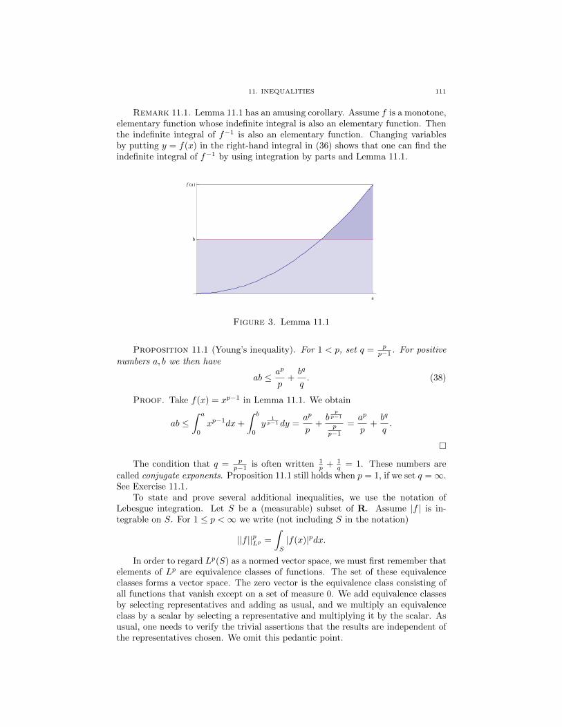
11. INEQUALITIES 111
Remark 11.1. Lemma 11.1 has an amusing corollary. Assume f is a monotone,elementary function whose indefinite integral is also an elementary function. Thenthe indefinite integral of f−1 is also an elementary function. Changing variablesby putting y = f(x) in the right-hand integral in (36) shows that one can find theindefinite integral of f−1 by using integration by parts and Lemma 11.1.
a
f Ha L
b
Figure 3. Lemma 11.1
Proposition 11.1 (Young’s inequality). For 1 < p, set q = pp−1 . For positive
numbers a, b we then have
ab ≤ ap
p+bq
q. (38)
Proof. Take f(x) = xp−1 in Lemma 11.1. We obtain
ab ≤∫ a
0
xp−1dx+
∫ b
0
y1p−1 dy =
ap
p+b
pp−1
pp−1
=ap
p+bq
q.
The condition that q = pp−1 is often written 1
p + 1q = 1. These numbers are
called conjugate exponents. Proposition 11.1 still holds when p = 1, if we set q =∞.See Exercise 11.1.
To state and prove several additional inequalities, we use the notation ofLebesgue integration. Let S be a (measurable) subset of R. Assume |f | is in-tegrable on S. For 1 ≤ p <∞ we write (not including S in the notation)
||f ||pLp =
∫S
|f(x)|pdx.
In order to regard Lp(S) as a normed vector space, we must first remember thatelements of Lp are equivalence classes of functions. The set of these equivalenceclasses forms a vector space. The zero vector is the equivalence class consisting ofall functions that vanish except on a set of measure 0. We add equivalence classesby selecting representatives and adding as usual, and we multiply an equivalenceclass by a scalar by selecting a representative and multiplying it by the scalar. Asusual, one needs to verify the trivial assertions that the results are independent ofthe representatives chosen. We omit this pedantic point.

112 3. FOURIER TRANSFORM ON R
We must also verify that || · ||Lp defines a norm. Property (2) from Definition2.1 of Chapter 2 is clear; property (1) of a norm is clear once we realize we areworking with equivalence classes. Property (3), the triangle inequality, is Theorem11.1 below. It is known as Minkowski’s inequality and is a subtle point. In orderto prove it, we first prove Holder’s inequality. See [S] both for additional versionsof this inequality and for some interesting historical discussion.
Proposition 11.2 (Holder’s inequality). Again assume 1 < p and q = pp−1 .
Assume |f |p is integrable on S and |g|q is integrable on S. Then |fg| is integrableon S and
||fg||L1 ≤ ||f ||Lp ||g||Lq . (39)
Proof. The result is obvious if either ||f ||Lp or ||g||Lq is zero. Otherwise, afterdividing f by ||f ||Lp and g by ||g||Lq , we may assume in (39) that each of thesenorms equals 1. For each x ∈ S, Young’s inequality implies
|f(x)g(x)| ≤ |f(x)|p
p+|g(x)|q
q. (40)
Integrating (40) shows that
||fg||L1 ≤||f ||pLpp
+||g||qLqq
=1
p+
1
q= 1.
Holder’s inequality remains true when p = 1, in which case it is obvious. (Ex-ercise 11.1)
Exercise 11.1. Verify Young’s inequality and Holder’s inequality when p = 1.
Exercise 11.2. Verify the statements from Remark 11.1.
Exercise 11.3. Suppose q = pp−1 . Show that ||hp−1||Lq = ||h||p−1
Lp .
Theorem 11.1 (Minkowski). Assume 1 ≤ p <∞. The triangle inequality holdsin Lp. In other words, if |f |p and |g|p are integrable, then |f + g|p is integrable and
||f + g||Lp ≤ ||f ||Lp + ||g||Lp . (41)
Proof. First we note that the statement is immediate if f + g = 0 and iseasy when p = 1. We thus assume p > 1 and that f + g is not the zero function(equivalence class). The following string of statements is elementary:
||f + g||pLp ≤∫
(|f |+ |g|) |f + g|p−1 =
∫|f | |f + g|p−1 +
∫|g||f + g|p−1. (42)
Now use Holder’s inequality in (42) to get
||f + g||pLp ≤ (||f ||Lp + ||g||Lp) || |f + g|p−1||Lq . (43)
Since q = pp−1 , the last term in (43) becomes || |f + g| ||p−1
Lp . (See Exercise 11.3.)
Dividing both sides by this term gives the triangle inequality (41).
Remark 11.2. The Lp spaces are complete; the proof requires results from thetheory of the Lebesgue integral.

11. INEQUALITIES 113
By Theorem 11.1, the Lp norm of a sum is at most the sum of the Lp norms.That result suggests that the Lp norm of an integral should be at most the integralthe Lp norms. Such a result holds; it is often called Minkowski’s inequality forintegrals. See [F1].
Next we use Holder’s inequality to establish the integral versions of Hilbert’sinequality and Hardy’s inequality, formulas (57.1) and (57.2) of Chapter 1. Notethat (44) is obvious when p = 1, as the right-hand side is infinite.
Theorem 11.2 (Hilbert’s inequality revisited). Let p, q be conjugate exponentswith p > 1. Assume that f ∈ Lp([0,∞)) and that g ∈ Lq([0,∞)). Then∫ ∞
0
∫ ∞0
f(x)g(y)
x+ ydxdy ≤ π
sin(πp )||f ||Lp ||g||Lq . (44)
Proof. Change variables in the integral in (44) by replacing x by yt. We get
I =
∫ ∞0
∫ ∞0
f(x)g(y)
x+ ydxdy =
∫ ∞0
∫ ∞0
f(yt)g(y)
1 + tdtdy. (45)
Let Ft denote the function given by Ft(y) = f(yt). Interchange the order of inte-gration in (45). Then apply Holder’s inequality to the inner integral, obtaining
I ≤∫ ∞
0
dt
1 + t||Ft||Lp ||g||Lq .
By changing variables, note that ||Ft||Lp = ||f ||Lp
t1p
. Plugging in this result gives
I ≤∫ ∞
0
dt
(1 + t)t1p
||f ||Lp ||g||Lq . (46)
The integral on the right-hand side of (46) equals πsin(πp ) , which gives (44). We
discuss the evaluation of the integral after the proof.
For p > 1, put Cp =∫∞
0dt
(t+1)t1p
. This integral can be evaluated by using
contour integrals and complex analysis. See for example page 133 in [D2] or pages157-8 in [A]. The contour used is pictured in Figure 3, where the positive real axisis a branch cut.
One can also reduce the computation of Cp (Exercise 11.4) to the Euler Betafunction discussed in Exercise 8.4 of Chapter 4 and the formula
Γ(z)Γ(1− z) =π
sin(πz). (47)
The best way to establish (47), however, uses contour integrals to evaluate Cp.
Exercise 11.4. For p > 1, put Cp =∫∞
0dt
(t+1)t1p
. Verify that
Cp =
∫ 1
0
s1p−1(1− s)
−1p ds. (48)
If you are familiar with the Gamma and Beta functions (See Chapter 4), show that
Cp = Γ(1
p)Γ(1− 1
p) =
π
sin(πp ).
The next exercise provides another generalization of Hilbert’s inequality. Forsimplicity we work in L2. To solve it, mimic the proof of Theorem 11.2.

114 3. FOURIER TRANSFORM ON R
|z|=Ε
|z|=R
Figure 4. Contour used to evaluate Cp
Exercise 11.5. Consider a continuous function K : (0,∞) × (0,∞) → [0,∞)
such that K(λx, λy) = K(x,y)λ . Show that∫ ∞
0
∫ ∞0
K(x, y)f(x)g(y)dxdy ≤ C||f ||L2 ||g||L2 ,
where C satisfies
C =
∫ ∞0
K(1, y)√y
dy.
The following beautiful exercise also fits into this general discussion, providinga bound from the other direction.
Exercise 11.6. Let xj be a sequence of distinct positive numbers. Considerthe infinite matrix A whose entries are 1
xj+xk. Prove that
0 ≤∑j,k
zjzkxj + xk
for all sequences zj , and equality holds only if z is the zero sequence. Thus A isnon-negative definite. Suggestion: Write
1
xj + xk=
∫ ∞0
e−(xj+xk)tdt.
Exercise 11.7. Suppose f = g, where g ≥ 0. Show that the matrix withentries f(xj − xk) is non-negative definite. Comment: The converse assertion is aspecial case of Bochner’s theorem.
Exercise 11.8. The Laplace transform of a function f is defined by
(Lf)(x) =
∫ ∞0
e−xtf(t)dt,
whenever the improper integral converges. Show that
(L2f)(x) =
∫ ∞0
f(t)
x+ tdt.

CHAPTER 4
Geometric considerations
The purpose of this chapter is to discuss various geometric problems which areinformed by orthogonality and related considerations. We begin with Hurwitz’sproof of the isoperimetric inequality using Fourier series. We prove Wirtinger’sinequality, both by Fourier series and by compact operators. We continue with atheorem comparing areas of the images of the unit disk under complex analyticmappings. We again give two proofs, one using power series and one using Green’s(Stokes’) theorem. The maps z → zd from the circle to itself play a prominentpart in our story. We naturally seek the higher dimensional versions of some ofthese results. It turns out, not surprisingly, that one can develop the ideas in manydirections. We limit ourselves here to a small number of possible paths, focusingon the unit sphere in Cn, and we travel only a small distance along each of them.
Complex analytic mappings sending the unit sphere in Cn to the unit spherein some CN play a major role in this Chapter. For example, we study polynomialmappings that are also invariant under finite subgroups of the unitary group, andwe discover a surprising connection to Chebyshev polynomials. We also computemany explicit integrals. The author’s technique of orthogonal homogenization isintroduced and is used to prove a sharp inequality about volumes (with multiplicityaccounted for) of complex analytic images of the unit ball. To prove this inequalitywe develop needed information about differential forms and complex vector fields.This material leads us to the Cauchy-Riemann (CR) geometry of the unit sphere.We close with a generalization of the Riesz-Fejer theorem on non-negative trigpolynomials to a result on Hermitian polynomials that are positive on the unitsphere. This Chapter thus provides many ways to extend results from the unitcircle to higher dimensions, all informed by orthogonality and Hermitian analysis.
We do not consider the Fourier transform in higher dimensions. Many bookson partial differential equations and harmonic analysis tell that story well.
1. The isoperimetric inequality
Geometric inequalities range from easy observations to deep assertions. One ofthe easiest such inequalities is that the rectangle of a given perimeter with maximumarea is a square. The proof follows from (x+y)(x−y) = x2−y2 ≤ x2, with equalitywhen y = 0. One of the most famous inequalities solves the isoperimetric problem;given a closed curve in the plane of length L, then the area A enclosed satisfies
A ≤ L2
4π . Equality happens only if the curve is a circle. We use Fourier series toprove this isoperimetric inequality, assuming that the curve is smooth.
Recall from calculus that a smooth planar curve is a smooth function γ : [a, b]→R2 for which γ′(t) does not vanish. Officially speaking, the curve is the function,but it is natural to think also of the curve as the image of the function, traced outin some order. The curve is called closed if γ(a) = γ(b) and simple if γ(t1) 6= γ(t2)
115

116 4. GEOMETRIC CONSIDERATIONS
for t1 6= t2 unless t1 = a, t2 = b or t1 = b, t2 = a. This complicated soundingcondition is clear in geometric terms; if one regards the curve as its image, thenthe curve is simple if it neither crosses itself nor covers itself multiple times. Note,for example, that the curve γ : [0, 2π] → C given by γ(t) = e2it is closed but notsimple, because it covers the circle twice.
The length of γ is the integral∫γds, where ds is the arc length form. In terms of
the function t 7→ γ(t), we have the equivalent formula L =∫ ba||γ′(t)||dt; this value
is unchanged if we reparametrize the curve. It is often convenient to parametrizeusing arc length; in this case ||γ′(s)|| = ||γ′(s)||2 = 1.
We can integrate 1-forms along nice curves γ. We give a precise definition of1-form in Section 5. For now we assume the reader knows the meaning of the lineintegral
∫γPdx + Qdy, assuming P and Q are continuous functions on γ. This
integral measures the work done in moving along γ against a force given by (P,Q).We also assume Green’s theorem from calculus. In Green’s theorem, the curve γ isassumed to be positively oriented. Intuitively, this condition means the (image ofthe) curve is traversed counter-clockwise as the parameter t increases from a to b.
Proposition 1.1 (Green’s theorem). Let γ be a piecewise smooth, positivelyoriented, simple closed curve in R2, bounding a region Ω. Assume that P and Qare continuously differentiable on Ω and continuous on Ω ∪ γ. Then∫
γ
Pdx+Qdy =
∫Ω
(∂Q
∂x− ∂P
∂y
)dxdy.
The area A enclosed by γ is of course given by a double integral. Assume thatγ is positively oriented. Using Green’s theorem, we see that A is also given by aline integral:
A =
∫Ω
dxdy =1
2
∫γ
xdy − ydx =1
2
∫ b
a
(x(t)y′(t)− x′(t)y(t)) dt. (1)
Notice the appearance of the Wronskian.
Exercise 1.1. Graph the set of points where x3 +y3 = 3xy. Use a line integralto find the area enclosed by the loop. Solve the same problem when the definingequation is x2k+1 + y2k+1 = (2k + 1)xkyk. Comment: Set y = tx to parametrizethe curve. Then xdy − ydx = x(tdx+ xdt)− txdx = x2dt.
Exercise 1.2. Verify Green’s theorem when Ω is a rectangle. Explain how toextend Green’s theorem to a region whose boundary consists of finitely many sides,each parallel to one of the coordinate axes.
Theorem 1.1 (Isoperimetric inequality, smooth version). Let γ be a smoothsimple closed curve in R2 of length L and enclosing a region of area A. Then
A ≤ L2
4π and equality holds only when γ defines a circle.
Proof. This proof goes back to Hurwitz in 1901. After a change of scalewe may assume that the length L of γ is 2π. After mapping [a, b] to [0, 2π] weparametrize by arc length s and thus assume γ : [0, 2π]→ R2 and ||γ′(s)|| = 1.

1. THE ISOPERIMETRIC INEQUALITY 117
Since the curve is closed, γ may be thought of as periodic of period 2π. Interms of Fourier series we may therefore write:
γ(s) = (x(s), y(s)) =
( ∞∑−∞
aneins,
∞∑−∞
bneins
)(2)
γ′(s) = (x′(s), y′(s)) =
( ∞∑−∞
inaneins,
∞∑−∞
inbneins
). (3)
Since (x′(s), y′(s)) is a unit vector, we have 2π =∫ 2π
0(x′(s))2 + (y′(s))2ds. The
only term that matters in computing the integral of a trigonometric series is theconstant term. Constant terms in x′(s)2 and y′(s)2 arise precisely when the termwith index n is multiplied by the term with index −n. It therefore follows that
∞∑−∞
n2(|an|2 + |bn|2) = 1. (4)
We do a similar computation of xy′ − yx′ to find the area A. We have
A =1
2
∣∣ ∫ 2π
0
(x(s)y′(s)− x′(s)y(s)) ds∣∣ =
1
22π∣∣∑ in(anbn − bnan)
∣∣= π|
∑in(anbn − bnan)| ≤ 2π
∑n|an||bn|. (5)
Next we use |n| ≤ n2 and
|anbn| ≤1
2(|an|2 + |bn|2) (6)
in the last term in (5). These inequalities and (4) yield
A ≤ π∑
n2(|an|2 + |bn|2) = π =L2
4π,
where we have also used the value L = 2π.We check when equality holds in the inequality. It must be that the only non-
zero terms are those with |n| = n2, that is n = 0,±1. We must also have equalityin (6), and hence |an| = |bn|. By (4) we then must have |a1| = |b1| = 1
2 . Put
a1 = 12eiµ and b1 = 1
2eiν . Since x(s) and y(s) are real, a−1 = a1 and b−1 = b1. In
other words we must have
(x(s), y(s)) =(a0 + a1e
is + a1e−is, b0 + b1e
is + b1e−is) .
Under these conditions we get (x − a0, y − b0) = (cos(s + µ), cos(s + ν)). Finally,remembering that (x′)2 + (y′)2 = 1, we conclude that cos(s + ν) = ±sin(s + µ).Hence γ defines a circle of radius 1.
Exercise 1.3. Given an ellipse E, create a family Et of ellipses such that thefollowing all hold:
(1) E = E0.(2) Each Et has the same perimeter.(3) The area enclosed by Et is nondecreasing as a function of t.(4) E1 is a circle.

118 4. GEOMETRIC CONSIDERATIONS
Exercise 1.4. A region Ω in the plane is convex if, whenever p, q ∈ Ω, the linesegment connecting p and q also lies in Ω. Assume that Ω is bounded, has a niceboundary, but is not convex. Find, by a simple geometric construction, a region Ω′
with the same perimeter as Ω but with a larger area. (Reflect a dent across a linesegment. See Figure 1.)
Figure 1. Convexity and the isoperimetric inequality
Remark 1.1. The isoperimetric inequality holds in higher dimensions. Forexample, of all simple closed surfaces in R3 with a given surface area, the sphereencloses the maximum volume.
2. Elementary L2 inequalities
In this section we prove several inequalities relating L2 norms of functions andtheir derivatives. The setting for the first example is an interval on the real line,whereas the setting for the second example is the unit disk in C.
We begin with the Wirtinger inequality, an easy one-dimensional version ofvarious higher dimensional inequalities relating functions and their derivatives. Wegive several proofs to help unify topics in this book.
Theorem 2.1 (Wirtinger inequality). Assume f is continuously differentiableon [0, 1] and f(0) = f(1) = 0. The following inequality holds and is sharp:
||f ||2L2 ≤1
π2||f ′||2L2 .
Proof. First we show that there is a function for which equality occurs. Putf(x) = sin(πx). Then ||f ′||2L2 = π2||f ||2L2 because
||f ||2L2 =
∫ 1
0
sin2(πx)dx =1
2
||f ′||2L2 =
∫ 1
0
π2cos2(πx)dx =π2
2.
Next we use Fourier series to prove the inequality. By putting f(−x) = −f(x),we extend f to be an odd function (still called f) on the interval [−1, 1]. Theextended f is still continuously differentiable, even at the endpoints. Then fequals its Fourier series, which involves only the functions sin(nπx). Put f(x) =

2. ELEMENTARY L2 INEQUALITIES 119∑cnsin(nπx). Since f is odd, c0 = f(0) = 0. Let L2 continue to denote L2([0, 1]).
By either the Parseval formula or by orthonormality we get
||f ||2L2 =1
2
∞∑−∞|cn|2 =
∞∑n=1
|cn|2
||f ′||2L2 =
∞∑n=1
n2π2|cn|2 = π2∞∑n=1
n2|cn|2.
Since 1 ≤ n2 for all n ≥ 1 we obtain
π2||f ||2L2 ≤ ||f ′||2L2 .
The proof also tells us when equality occurs! Put cn = 0 unless n = 1; that is, putf(x) = sin(πx).
Sin(Πx)
-1.0 -0.5 0.5 1.0
-1.0
-0.5
0.5
1.0
Figure 2. Wirtinger inequality
Proof. We sketch a different proof using compact operators. Define a linearoperator T on the continuous functions in L2([0, 1]) by Tf(x) =
∫ x0f(t)dt. We
work on the subspace where f(0) = f(1) = 0. Computation (see Exercise 1.7)
shows that T ∗f(x) =∫ 1
xf(u)du. The operator T ∗T is compact and self-adjoint.
It is easy to check that each eigenvalue of T ∗T is non-negative. By the first partof the proof of the Spectral theorem, the maximal eigenvalue λM of T ∗T satisfiesλM = ||T ∗T || = ||T ||2. We find all eigenvalues.
Set T ∗Tf = λf to get ∫ 1
x
∫ t
0
f(u)dudt = λf(x).
Differentiating twice and using the fundamental theorem of calculus gives
−f(x) = λf ′′(x).
Since f(0) = f(1) = 0 we conclude that f(x) = c sin( x√λ
), where 1√λ
= nπ. Thus
λ = 1n2π2 . The maximum happens when n = 1. We get ||T ||2 = 1
π2 , which is

120 4. GEOMETRIC CONSIDERATIONS
equivalent to saying that ||Tg||L2 ≤ 1π ||g||L2 for all g. Setting g = f ′ gives the
desired conclusion.
Corollary 2.1. Assume f is continuously differentiable with f(a) = f(b) = 0.Then ∫ b
a
|f(x)|2dx ≤ (b− aπ
)2
∫ b
a
|f ′(x)|2dx.
Proof. The result follows from changing variables (Exercise 2.2).
Exercise 2.1. Put Tf(x) =∫ baK(x, y)f(y)dy. Express T ∗ as an integral
operator. Check your answer when T is as in the proof of Theorem 2.1.
Exercise 2.2. Prove Corollary 2.1.
Higher dimensional analogues of the Wirtinger inequality are called Poincareinequalities. Given a region Ω in Rn, a Poincare inequality is an estimate of theform (for some constant C)
||u||2L2 ≤ C2
(∣∣∣∣∫Ω
u
∣∣∣∣2 + ||∇u||2L2
). (P )
Let A denote the volume of Ω and let u0 = 1A
∫Ωu denote the average value of u
on Ω. We can rewrite (P) in the form
||u− u0||2L2 ≤ ||∇u||2L2 . (P.1)
By expanding the squared norm on the left-hand side of (P.1) and doing somesimple manipulations, we can also rewrite (P) in the form
||u||2L2 ≤1
A
∣∣∣∣∫ u
∣∣∣∣2 + C2||∇u||2L2 . (P.2)
The technique of subtracting the average value and expanding the squared normappears, in various guises, many times in this book. For example, this reasoningis standard in elementary probability, as used in Proposition 6.1 of the Appendix.Observe also, for f, f0 in a Hilbert space, that
||f − f0||2 = ||f ||2 − ||f0||2
whenever f = f0 ⊕ g. This version of the Pythagorean theorem was used in theproof of Bessel’s inequality, where f0 was the orthogonal projection of f onto thesubspace spanned by a finite orthonormal system.
Poincare estimates do not hold for all domains. When such an inequality doeshold, the smallest value of C that works is called the Poincare constant for thedomain.
We make one additional observation. In our proof of the Wirtinger inequality,we assumed that f vanished at both endpoints. We could have assumed that fvanished at only one endpoint, or instead that the average value of f was 0, and ineach case proved similar results. The condition that the average value of f vanishesmeans that f is orthogonal to the one-dimensional subspace of constant functions.The condition that f vanish at the endpoints means that f lies in a subspace ofcodimension two.
Exercise 2.3. Find the Poincare constant for the interval [−A,A]. (The func-tion sin( πx2A ) achieves the bound. The answer is 2A
π .)

2. ELEMENTARY L2 INEQUALITIES 121
Remark 2.1. The Wirtinger inequality provides a bound on the L2 norm of afunction in terms of the L2 norm of its derivative. Various inequalities that boundthe maximum of the derivative p′ of a polynomial in terms of the maximum of p(thus going in the other direction) and its degree are called Bernstein inequalitiesand Markov inequalities. We do not consider such results in this book.
We next prove a simple geometric inequality in one complex dimension. Itmotivates a more difficult higher dimensional analogue which we prove in Section9. The orthogonality of the functions einθ again features prominently.
Let f be a complex analytic function on the unit disk B1. Let Af denote thearea of the image, with multiplicity counted. For example, if f(z) = zm, then fcovers the disk m times and Af = mπ. The formula for Af involves the L2 normof the derivative. We make the concept of counting multiplicity precise by definingAf as follows:
Definition 2.1. Let Ω be open in C. Assume f : Ω→ C is complex analytic.The area, written Af (Ω) or Af , of the image of f , with multiplicity counted, isdefined by
Af = ||f ′||2L2(Ω). (7)
We next note that this concept agrees with what we expect when f is injective.
Lemma 2.1. Let f : Ω → C be complex analytic and injective. Then the areaof f(Ω) equals ||f ′||2L2(Ω).
Proof. Let A(f) denote the area of the image of f . Write f = u+iv and defineF (x, y) = (u(x, y), v(x, y)). The Cauchy-Riemann equations and the definition off ′ imply det(F ′) = uxvy − uyvx = u2
x + u2y = |f ′|2. Since F is injective, the change
of variables formula for double integrals applies and gives
A(f) =
∫F (Ω)
dudv =
∫Ω
|det(F ′)|dxdy =
∫Ω
|f ′(z)|2dxdy = ||f ′||2L2 .
Versions of the change of variables formula hold more generally. For example,suppose that f is m-to-one for some fixed m. The change of variables formula gives
m
∫F (Ω)
dudv =
∫Ω
|det(F ′)|dxdy =
∫Ω
|f ′(z)|2dxdy = ||f ′||2L2 .
In general, the multiplicity varies from point to point. For complex analytic func-tions, things are nonetheless quite nice. See [A] for the following result. Supposethat f is complex analytic near z0 and the function z → f(z)− f(z0) has a zero oforder m. Then, for w sufficiently close to f(z0), there is a (deleted) neighborhoodof z0 on which the equation f(z) = w has precisely m solutions. By breaking Ωinto sets on which f has constant multiplicity, we justify the definition of Af .
We return to the unit disk. The natural Hilbert space here is the set A2 ofsquare-integrable complex analytic functions f on the unit disk. The inner producton A2 is given by
〈f, g〉 =
∫B1
f(z)g(z)dxdy.
We are also concerned with the subspace of A2 consisting of those f for which f ′
is square integrable.

122 4. GEOMETRIC CONSIDERATIONS
Lemma 2.2. The functions zn for n = 0, 1, 2, ... form a complete orthogonalsystem for A2.
Proof. Using polar coordinates we have
〈zn, zm〉 =
∫ 1
0
∫ 2π
0
rn+m+1ei(n−m)θdθdr. (8)
By (8), the inner product vanishes unless m = n. To check completeness, we observethat a complex analytic function in the unit disk has a power series based at 0 thatconverges in the open unit disk. If f is orthogonal to each monomial, then eachTaylor coefficient of f vanishes and f is identically 0.
In Proposition 2.1 we relate ||f ||2L2 to the l2 norm of the Taylor coefficientsof f . By (9) below we can identify elements of A2 with sequences bn such that∑ |bn|2
n+1 converges.
Consider the effect on the area of the image if we multiply f by z. Since |z| < 1,the inequality |zf(z)| ≤ |f(z)| is immediate. But the area of the image under zfexceeds the area of the image under f , unless f is identically 0. In fact we canexplain and determine precisely how the area grows.
Proposition 2.1. Let f(z) =∑∞n=0 bnz
n be a complex analytic function onthe unit disk B1. We assume that both f and f ′ are in L2(B1). Then
||f ||2L2 = π
∞∑n=0
|bn|2
n+ 1(9)
||f ′||2L2 = π
∞∑n=0
(n+ 1)|bn+1|2 (10)
||(zf)′||2L2 = ||f ′||2L2 + π
∞∑n=0
|bn|2. (11.1)
Thus Azf ≥ Af and equality occurs only when f vanishes identically.
Proof. The proof of (9) is an easy calculation in polar coordinates, using theorthogonality of einθ. Namely, we have
||f ||2L2 =
∫B1
|∑
bnzn|2dxdy =
∫ 1
0
∫ 2π
0
∑bnbmr
m+neiθ(m−n)rdrdθ.
The only terms that matter are those for which m = n and we see that
||f ||2L2 = 2π∑|bn|2
∫ 1
0
r2n+1dr = π
∞∑n=0
|bn|2
n+ 1.
Formula (10) follows immediately from (9). To prove (11.1) observe that (zf)′(z) =∑∞n=0(n+ 1)bnz
n. By (10) we have
||(zf)′||2L2 = π
∞∑n=0
(n+ 1)|bn|2 = π
∞∑n=0
n|bn|2 + π
∞∑n=0
|bn|2
= ||f ′||2L2 + π
∞∑n=0
|bn|2.

2. ELEMENTARY L2 INEQUALITIES 123
We express (11.1) in operator-theoretic language. Let D = ddz with domain
f ∈ A2 : f ′ ∈ A2. Then D is an unbounded linear operator. Let M denotethe bounded operator of multiplication by z. When f extends continuously to thecircle, we write Sf for its restriction to the circle, that is, its boundary values. Thus
||Sf ||2 = 12π
∫ 2π
0|f |2. The excess area has a simple geometric interpretation:
Corollary 2.2. Suppose Mf is in the domain of D. Then Sf is square-integrable on the circle and
||DMf ||2L2 − ||Df ||2L2 =1
2
∫ 2π
0
|f(eiθ)|2dθ = π||Sf ||2. (11.2)
Proof. The result is immediate from (11.1).
Corollary 2.2 suggests an alternate way to view (11.1) and (11.2). We canuse Green’s theorem to relate the integral over the unit disk to the integral overthe circle. The computation uses the notation of differential forms. We discussdifferential forms in detail in Sections 5 and 6. For now we need to know less. Inparticular dz = dx+ idy and dz = dx− idy. The area form becomes
dx ∧ dy =−1
2idz ∧ dz =
i
2dz ∧ dz.
If f is complex analytic, then ∂f = 0 (the Cauchy-Riemann equations) and we have
df = (∂ + ∂)f = ∂f = f ′(z)dz.
Finally, we use Green’s theorem, expressed in complex notation, in formula (12) ofthe geometric proof below. We generalize this proof in Section 9.
Exercise 2.4. Express Green’s theorem in complex notation: express the lineintegral of Adz +Bdz around γ as an area integral over the region bounded by γ.
Exercise 2.5. Use the previous exercise to show that∫γf(z)dz = 0 when f is
complex analytic and γ is a closed curve as in Green’s theorem.
Here is a beautiful geometric proof of (11.2):
Proof. For any complex analytic f we have
Af = ||f ′||2L2 =i
2
∫B
∂f ∧ ∂f =i
2
∫B
d(f∂f).
We apply this formula also to (zf)′. The difference in areas satisfies
Azf −Af = ||(zf)′||2L2 − ||f ′||2L2 =i
2
∫B
d(zf∂(zf)− f∂f
).
Using Green’s theorem, we rewrite this integral as an integral over the circle:
Azf −Af =i
2
∫S1
zf∂(zf)− (f∂f). (12)
By the product rule, ∂(zf) = fdz + z∂f . We plug this formula into (12) andsimplify, getting
Azf −Af =i
2
∫S1
(|z|2 − 1)f∂f +i
2
∫S1
z|f(z)|2dz.

124 4. GEOMETRIC CONSIDERATIONS
The first integral vanishes because |z|2 = 1 on the circle. We rewrite the secondintegral by putting z = eiθ to obtain
i
2
∫S1
eiθ|f(eiθ)|2(−i)e−iθdθ =1
2
∫S1
|f(eiθ)|2dθ = π1
2π
∫S1
|f(eiθ)|2dθ = π||Sf ||2.
-0.5 0.5 1.0
-1.0
-0.5
0.5
1.0
Figure 3. Injective image of unit disk
-0.5 0.5 1.0
-1.0
-0.5
0.5
1.0
Figure 4. Overlapping image of unit disk
Exercise 2.6. Show that Corollary 2.2 can be stated as M∗D∗DM −D∗D =πS∗S.
Exercise 2.7. What are the eigenfunctions and eigenvalues of DM and ofMD? Show that the commutator [D,M ] = DM − MD is the identity. Thisexample arises in quantum mechanics.
Exercise 2.8. Find a closed formula for∑∞j=0
|z|2jcj
, where cj = ||zj ||2 is the
squared norm in A2. The answer is the Bergman kernel function of the unit disk.

3. UNITARY GROUPS 125
Exercise 2.9. For 0 ≤ a ≤ 1 and for |z| < 1, put fa(z) =√
1− a2z + az2.Find ||f ′a||2L2 in terms of a. For several values of a, graph the image of the unit diskunder f . For what values of a is f injective? See Figures 3 and 4.
Exercise 2.10. Put f(z) = z + z2 + z3. Describe or graph the image of theset |z| = r under f for several values of r. Suggestion: Use polar coordinates.
3. Unitary groups
We now begin studying geometric problems in several complex variables. Recallthat 〈z, w〉 denotes the Hermitian inner product of points in complex Euclideanspace Cn. The unitary group U(n) consists of the linear transformations T whichpreserve the inner product; 〈Tz, Tw〉 = 〈z, w〉. Setting z = w shows that suchtransformations also preserve norms. The converse is also true: if ||Tz||2 = ||z||2for all z, then 〈Tz, Tw〉 = 〈z, w〉 for all z and w by Proposition 7.2 of Chapter 2.
The group law in U(n) is composition. Let U, V be unitary transformations onCN . Then the composition UV is also unitary, because
(UV )∗ = V ∗U∗ = V −1U−1 = (UV )−1.
It follows that the collection U(N) of unitary transformations on CN is a subgroupof the group of invertible linear transformations.
We will occasionally deal with complex Euclidean spaces of different dimen-sions. It is convenient to omit the dimension in the notation for the inner productsand norms. For example, suppose L : Cn → Cn+1 is given by L(z) = (z, 0). ThenL is linear and ||L(z)|| = ||z||, but L is not unitary. Distance preserving maps arecalled isometries.
Our first result (which holds much more generally than we state here) providesa polarization technique and gets used several times in the sequel. We use it severaltimes in the special case when f and g are polynomial mappings.
Theorem 3.1. Let B be a ball centered at 0 in Cn. Suppose f : B → CN1
and g : B → CN2 are complex analytic mappings. and ||f(z)||2 = ||g(z)||2 for allz ∈ B. Assume that the image of g lies in no lower dimensional subspace, and thatN1 ≥ N2. Then there is an isometry U : CN2 → CN1 such that f(z) = Ug(z) forall z. When N2 = N1, U is unitary.
Proof. We expand f and g as convergent power series about 0, writing f(z) =∑αAαz
α and g(z) =∑αBαz
α; the coefficients Aα lie in CN1 and the Bα lie inCN2 . Equating the Taylor coefficients in ||f(z)||2 = ||g(z)||2 leads, for each pair αand β of multi-indices, to
〈Aα, Aβ〉 = 〈Bα, Bβ〉. (13)
It follows from (13) that Aα1, . . . , AαK is a linearly independent set if and only if
Bα1, . . . , BαK is a linearly independent set. We then define U by U(Bα) = Aα for a
maximal linearly independent set of the Bα. If Bµ is a linear combination of someBα, then we define U(Bµ) as the same linear combination of the Aα. The relations(13) guarantee that U is well-defined. Furthermore, these relationships guaranteethat U preserves inner products. Hence U is an isometry on the span of the Bα.When N1 = N2, an isometry U must be unitary.
126 4. GEOMETRIC CONSIDERATIONS
Example 3.1. The parallelogram law provides an example of Theorem 1. Sup-pose g(z1, z2) = (
√2z1,√
2z2) and f(z1, z2) = (z1 + z2, z1 − z2). Then
||g(z)||2 = 2|z1|2 + 2|z2|2 = |z1 + z2|2 + |z1 − z2|2 = ||f(z)||2.In this case f = Ug, where U is given by
U =
(1√2
1√2
1√2
−1√2
).
Let us now consider the geometry of the unit sphere, which admits many sym-metries. For example, if eiθ lies on the unit circle S1, and z lies on the unit sphereS2n−1, the scalar multiple eiθz lies on S2n−1 as well. Thus S1 acts on S2n−1. Wecan replace S1 with the n-torus S1× ...×S1. In this case we map z = (z1, z2, ..., zn)to (eiθ1z1, e
iθ2z2, ..., eiθnzn). These maps are examples of a general situation, in
which we consider subgroups of the group of complex analytic automorphisms ofthe sphere. Rather than considering the full group, we will focus on the unitarygroup U(n) and its finite subgroups. Various interesting combinatorial and number-theoretic issues arise in this setting.
We start in one dimension with an elementary identity (Lemma 3.1) involvingroots of unity. The proof given reveals the power of geometric reasoning; one canalso prove this identity by factoring 1− tm over the complex numbers.
Definition 3.1. A complex number ω is called a primitive m-th root of unityif ωm = 1 and m is the smallest such positive integer.
For example, the imaginary unit i is a primitive fourth root of unity. Givena primitive m-th root of unity ω, the powers ωj for j = 0, 1, ...,m − 1 are equallyspaced on the unit circle. These m points define a cyclic subgroup of the unit circleof order m. Note that the inverse of ω is ωm−1, which also equals ω. Note also thatS1 = U(1).
Lemma 3.1. Let ω be a primitive m-th root of unity. Then
1−m−1∏j=0
(1− ωjt) = tm. (14)
Proof. The expression on the left-hand side is a polynomial in t of degree m.It is invariant under the map t → ωt. The only invariant monomials of degree atmost m are constants and constants times tm. Hence this expression must be ofthe form α + βtm. Setting t = 0 shows that α = 0 and setting t = 1 shows thatβ = 1.
This proof relies on the cyclic subgroup Γm of the unit circle, or of U(1), gen-erated by ω. We will generalize this lemma and related ideas to higher dimensions,where things become more interesting.
Let Γ be a finite subgroup of U(n). The analogue of the left-hand side of (14)is the following Hermitian polynomial:
ΦΓ(z, ζ) = 1−∏γ∈Γ
(1− 〈γz, ζ〉). (15)
One can show (we do not use the result, and hence we omit the proof) that ΦΓ isuniquely determined by the following properties:
3. UNITARY GROUPS 127
(1) ΦΓ is Hermitian symmetric.(2) ΦΓ(0, 0) = 0.(3) ΦΓ is Γ-invariant.(4) ΦΓ(z, z) is of degree in z at most the order of Γ.(5) ΦΓ(z, z) = 1 for z on the unit sphere.
In the special case when Γ is the group generated by a primitive m-th root ofunity times the identity operator, (14) generalizes to the identity (16):
1−m−1∏j=0
(1− ωj
n∑k=1
tk
)=
(n∑k=1
tk
)m=∑|α|=m
(m
α
)tα. (16)
In this case the multinomial coefficients(mα
)make an appearance:(
m
α
)=
m!
α1! . . . αn!.
See Sections 4 and 8 for more information about multi-index notation and themultinomial theorem, which is the far right equality in (16).
Interesting generalizations of (16) result from more complicated representationsof cyclic groups. The product in (17) gives one collection of non-trivial examples:
1−m−1∏j=0
(1−
n∑k=1
ωkjtk
). (17)
The coefficients of the expansion are integers with many interesting properties.
Exercise 3.1. Prove Lemma 3.1 by factoring 1− tm.
Exercise 3.2. Prove that ΦΓ(z, w) is Hermitian symmetric (Definition 3.2 ofChapter 1).
Exercise 3.3. Let R(z, z) =∑α,β cα,βz
αzβ be a Hermitian symmetric poly-
nomial. Prove that there are linearly independent polynomials Aj(z) and Bk(z)such that
R(z, z) =∑j
|Aj(z)|2 −∑k
|Bk(z)|2 = ||A(z)||2 − ||B(z)||2.
Exercise 3.4. Write ΦΓ = ||A||2 − ||B||2 as in the previous exercise. Showthat we may choose A and B to be Γ-invariant.
In the rest of this section we consider several cyclic subgroups of U(2). Write(z, w) for a point in C2. Let η be a primitive p-th root of unity. We next study themapping ΦΓ when Γ = Γ(p, q) is the cyclic group of U(2) of order p generated bythe matrix (
η 00 ηq
).
Remark 3.1. The quotient space S3/Γ(p, q) is called a lens space. Thesespaces are important in topology.
The definition of ΦΓ(p,q) yields
ΦΓ(p,q) = 1−p−1∏j=0
(1− ηj |z|2 − ηqj |w|2).

128 4. GEOMETRIC CONSIDERATIONS
This expression depends only upon the expressions |z|2 and |w|2; we simplify nota-tion by defining the polynomial fp,q(x, y) by
fp,q(x, y) = 1−p−1∏j=0
(1− ηjx− ηqjy). (18)
By taking j = 0 in the product, it follows that fp,q(x, y) = 1 on the line x+ y = 1.
Lemma 3.2. fp,1(x, y) = (x+ y)p.
Proof. The result follows by replacing t by x+ y in Lemma 3.1.
The (binomial) coefficients of fp,1 are integers which satisfy an astonishingnumber of identities and properties. More is true. For each q, the coefficients offp,q are also integers, and they satisfy many interesting combinatorial and number-theoretic properties as well. We mention one of the properties now. Most peopleknow the so-called freshman’s dream, that (x+ y)p ≡ xp + yp modulo p if and onlyif p is prime. The same result holds for each fp,q, although we omit the proof here.
The polynomials fp,2 are more complicated than fp,1 = (x + y)p. When p isodd, all the coefficients of fp,2 are non-negative. Here are the first few fp,2:
f1,2(x, y) = x+ y
f2,2(x, y) = x2 + 2y − y2
f3,2(x, y) = x3 + 3xy + y3
f4,2(x, y) = x4 + 4x2y + 2y2 − y4
f5,2(x, y) = x5 + 5x3y + 5xy2 + y5. (19)
We can find all these polynomials by solving a single difference equation. Weoffer two proofs of the following explicit formula for fp,2. The key idea in the firstproof is to interchange the order in a double product.
Proposition 3.1. For all non-negative integers p we have
fp,2(x, y) = (x+
√x2 + 4y
2)p + (
x−√x2 + 4y
2)p − (−y)p. (20)
Proof. Set q = 2 in (18). We regard the expression as the product of variousquadratics in η, as follows:
1− f(x, y) =
p−1∏j=0
(1− ηjx− η2jy) =
p−1∏j=0
(1− c1(x, y)ηj)(1− c2(x, y)ηj)
=
p−1∏j=0
(1− c1(x, y)ηj)
p−1∏j=0
(1− c2(x, y)ηj).
Here c1 and c2 are the reciprocals of the roots of the quadratic 1− xη− yη2. Eachof the two products is familiar from Lemma 3.1. Using that result we obtain
1− f(x, y) = (1− c1(x, y)p)(1− c2(x, y)p).
It follows that f has the following expression in terms of the cj :
f(x, y) = c1(x, y)p + c2(x, y)p − (c1(x, y)c2(x, y))p.
3. UNITARY GROUPS 129
The product c1(x, y)c2(x, y) equals −y. The sum c1(x, y)+c2(x, y) equals x. Solvingthis system for c1 and c2 using the quadratic formula determines the expressionsarising in (20).
We sketch a second proof based on recurrence relations.
Proof. (Sketch). It follows by setting x = 0 in formula (18) that the term−(−y)p appears in fp,2. Let gp(x, y) denote the other terms. The recurrencerelation gp+2(x, y) = xgp+1(x, y) + ygp(x, y) also follows from (18). To solve thisrecurrence, we use the standard method. The characteristic equation is λ2−xλ−y =
0. Its roots arex±√x2+4y
2 . Using the initial conditions that g1(x, y) = x and
g2(x, y) = x2+2y we determine gp(x, y). Adding in the term−(−y)p yields (20).
These polynomials are related to some classical mathematics.
Definition 3.2. The n-th Chebyshev polynomial Tn is defined by
Tn(x) = cos(n cos−1(x)).
Although it is not instantly obvious, the n-th Chebyshev polynomial is a poly-nomial of degree n. Hence these polynomials are linearly independent.
Example 3.2. The first few Chebyshev polynomials:
• T0(x) = 1• T1(x) = x• T2(x) = 2x2 − 1• T3(x) = 4x3 − 3x• T4(x) = 8x4 − 8x2 + 1• T5(x) = 16x5 − 20x3 + 5x.
Exercise 3.5. Verify that Tn(x) is a polynomial. (See Exercise 3.7 for oneapproach.) Verify the formulas for Tj(x) for j = 1, 2, 3, 4, 5.
Remark 3.2. The polynomials Tn(x) are eigenfunctions of a Sturm-Liouvilleproblem. The differential equation, (SL) from Chapter 2, is (1−x2)y′′−xy′+λy = 0.The Tn are orthogonal on the interval [−1, 1] with respect to the weight functionw(x) = 1√
1−x2. By Theorem 11.2 of Chapter 2, they form a complete orthogonal
system for L2([−1, 1], w).
Exercise 3.6. Verify that Tn is an eigenfunction as described in the remark;what is the corresponding eigenvalue λ?
Proposition 3.2. The fp,2 have the following relationship to the Chebyshevpolynomials Tp(x):
fp,2(x,−1
4) + (
1
4)p = 21−p (cos(p cos−1(x))
)= 21−pTp(x).
Proof. See Exercise 3.7.
It is remarkable that our considerations of group-invariant mappings connectso closely with classical mathematics. The polynomials fp,2 arise for additionalreasons in several complex variables. When p is odd, all the coefficients of fp,2 arenon-negative. Put x = |z|2 and y = |w|2 and write p = 2r + 1. Then
f2r+1,2(|z|2, |w|2) =∑b
cb|z|2(2r+1−2b)|w|2b = ||g(z, w)||2.
130 4. GEOMETRIC CONSIDERATIONS
Since f2r+1,2(x, y) = 1 on x+ y = 1 we see that ||g(z, w)||2 = 1 on the unit sphere.Hence g(z, w) maps the unit sphere S3 to the unit sphere S2N−1, where N = r+ 2.Thus g provides a far from obvious example of a group-invariant mapping betweenspheres.
The functions fp,q satisfy an extremal property. If a polynomial f of degree din x, y has N terms, all non-negative coefficients, and f(x, y) = 1 on x + y = 1,then the inequality d ≤ 2N − 3 holds and is sharp. Equality holds for the f2r+1,2.
Exercise 3.7. Prove Proposition 3.2. Suggestion. First find a formula for
cos−1(s) using cos(t) = eit+e−it
2 = s and solving a quadratic equation for eit.
Exercise 3.8. Show that Tnm(x) = Tn(Tm(x)).
Exercise 3.9. Find a formula for the generating function∑∞n=0 Tn(x)tn. Do
the same for∑∞n=0 fn,2(x, y)tn.
The next exercise is intentionally a bit vague. See [D3] and the references therefor considerably more information.
Exercise 3.10. Use Mathematica or something similar to find fp,3 and fp,4for 1 ≤ p ≤ 11. See what you can discover about these polynomials.
4. Proper mappings
Consider the group-invariant polynomial (15) above when ζ = z. The factor1 − 〈γz, z〉 vanishes on the sphere when γ is the identity of the group. HenceΦΓ(z, z) = 1 when z is on the sphere. By Exercises 3.2 and 3.3, we may write
ΦΓ(z, z) =∑j
|Aj(z)|2 −∑k
|Bk(z)|2 = ||A(z)||2 − ||B(z)||2
where the polynomials Aj and Bk are invariant. If B = 0, (thus ΦΓ is a squarednorm), then ΦΓ will be an invariant polynomial mapping between spheres. If B 6= 0,then the target is a hyperquadric.
The group-invariant situation, where the target is a sphere, is completely un-derstood and beautiful. It is too restrictive for our current aims. In this section wetherefore consider polynomial mappings between spheres, without the assumptionof group-invariance.
In one dimension, the functions z 7→ zm have played an important part in ourstory. On the circle, of course, zm = eimθ. The function z 7→ zm is complex analyticand maps the unit circle S1 to itself. One of many generalizations of these functionsto higher dimensions results from considering complex analytic functions sendingthe unit sphere S2n−1 into some unit sphere, perhaps in a different dimension. Wediscuss these ideas here and relate them to the combinatorial considerations fromthe previous section.
Definition 4.1. Let Ω and Ω′ be open, connected subsets of complex Euclideanspaces. Suppose f : Ω → Ω′ is continuous. Then f is called proper if, wheneverK ⊂ Ω′ is compact, then f−1(K) is compact in Ω.
Lemma 4.1. A continuous map f : Ω→ Ω′ between bounded domains is properif and only if the following holds: whenever zν is a sequence tending to the bound-ary bΩ, then f(zν) tends to bΩ′.

4. PROPER MAPPINGS 131
Proof. We prove both statements by proving their contrapositives. First letzν tend to bΩ. If f(zν) does not tend to bΩ′, then it has a subsequence whichstays in a compact subset K of Ω′. But then f−1(K) is not compact, and f isnot proper. Thus properness implies the sequence property. Now suppose f is notproper. Find a compact set K such that f−1(K) is not compact in Ω. Then thereis a sequence zν in f−1(K) tending to bΩ, but the image sequence stays withina compact subset K.
Lemma 4.1 states informally that f is proper if, whenever z is close to bΩ, thenf(z) is close to bΩ′. Hence it has an ε−δ version which we state and use only whenΩ and Ω′ are open unit balls.
Corollary 4.1. A continuous map f : Bn → BN is proper if and only if, forall ε > 0 there is a δ > 0 such that 1− δ < ||z|| < 1 implies 1− ε < ||f(z)|| < 1.
Our main interest is complex analytic mappings between spheres, especiallysuch polynomial mappings. For complex analytic mappings, the maximum principleimplies that a nonconstant mapping sending the unit sphere to some unit spheremust actually be a proper mapping from ball to ball. On the other hand, a (complexanalytic) polynomial mapping between balls is also defined on the boundary sphere,and Lemma 4.1 implies that such mappings send the boundary to the boundary. Itwould thus be possible never to mention the term proper map and we could still doeverything we are going to do. We continue to work with proper mappings becauseof the intuition they provide.
Remark 4.1. Proper complex analytic mappings must be finite-to-one, al-though not all points in the image must have the same number of inverse images.By definition of proper, the inverse image of a point must be a compact set. Be-cause of complex analyticity, the inverse image of a point must also be a complexvariety. Together these facts show that no point in the target can have more thana finite number of inverse images.
Exercise 4.1. Which of the following maps are proper from R2 → R?
(1) f(x, y) = x2 + y2
(2) g(x, y) = x2 − y2
(3) h(x, y) = x.
Exercise 4.2. Under what circumstances is a linear map L : Cn → CN
proper?
Our primary concern will be complex analytic proper mappings between balls.We start with the unit disk B1 contained in C. Let us recall a simple version ofthe maximum principle. Suppose f is complex analytic in the open unit disk B1,and |f(z)| ≤M on the boundary of a closed set K. Then the same estimate holdsin the interior of K.
Proposition 4.1. Suppose f : B1 → B1 is complex analytic and proper. Thenf is a finite Blaschke product: there are points a1, ..., ad in the unit disk, possiblyrepeated, and a point eiθ on the circle, such that
f(z) = eiθd∏j=1
aj − z1− ajz
.
132 4. GEOMETRIC CONSIDERATIONS
If also either f−1(0) = 0 or f is a polynomial, then f(z) = eiθzm for some positiveinteger m.
Proof. Because f is proper, the set f−1(0) is compact. We first show thatit is not empty. If it were empty, then both f and 1
f would be complex analytic
on the unit disk, and the values of 1|f(z)| would tend to 1 as z tends to the circle.
The maximum principle would then force | 1f(z) | ≤ 1 on the disk, which contradicts
|f(z)| < 1 there.Thus the compact set f−1(0) is not empty. Because f is complex analytic, this
set must be discrete. Therefore it is finite, say a1, ..., ad (with multiplicity allowed).
Let B(z) denote the product∏ aj−z
1−ajz . We show that z 7→ f(z)B(z) is a constant map
of modulus one. Then f = eiθB.By Corollary 4.1, applied to both f and B, for each ε > 0 we can find a δ > 0
such that 1 − ε < |f(z)| ≤ 1 and 1 − ε < |B(z)| ≤ 1 for |z| > 1 − δ. It followsby the maximum principle that these estimates hold for all z with |z| ≤ 1 − δ as
well. The function g = fB is complex analytic in the disk, as the zeros of B and
of f correspond and thus cancel in g. By the maximum principle applied to g, wehave for all z that 1 − ε < |g(z)| < 1
1−ε . Since ε is arbitrary, we may let ε tend to
0 and conclude that |g(z)| = 1. It follows (by either Theorem 3.1 or the maximumprinciple) that g is a constant eiθ of modulus one. Thus f(z) = eiθB(z).
Exercise 4.3. Suppose f : B1 → B1 is complex analytic and proper. Findanother proof that there is a z with f(z) = 0. One possible proof composes f withan automorphism of the disk, preserving properness while creating a zero.
Consider next the proper complex analytic self-mappings of the unit ball Bn inCn for n ≥ 2. We do not prove the following well known result in several complexvariables: the only proper complex analytic maps from the unit ball Bn to itself(when n ≥ 2) are automorphisms. These mappings are analogues of the individualfactors in Proposition 4.1. They have the form
f(z) =z − La(z)
1− 〈z, a〉. (20)
Here La is a linear transformation depending on a, for a an arbitrary point in Bn.The only such polynomial examples are the unitary mappings f(z) = Uz. In orderto obtain analogues of z → zd we must increase the target dimension.
Definition 4.2. Let f = (f1, ..., fM ) and g = (g1, ..., gN ) be mappings takingvalues in CM and CN . Their tensor product f ⊗ g is the mapping taking values inCMN defined by (f1g1, ..., fjgk, ..., fMgN ).
In Definition 4.2 we did not precisely indicate the order in which the terms figjare listed. The reason is that we do not care; nearly everything we do in this sectionregards h and Lh as the same, whenever L is a permutation matrix. The followingobvious formula suggests why the tensor product is relevant to proper mappingsbetween balls:
||f ⊗ g||2 = ||f ||2||g||2. (21)
Let m be a positive integer. We write z⊗m for the tensor product of the identitymap with itself m times. It follows immediately from (21) that ||z⊗m||2 = ||z||2m;

4. PROPER MAPPINGS 133
in particular the polynomial map z 7→ z⊗m takes the unit sphere in its domainto the unit sphere in its target. It exhibits many of the properties satisfied bythe mapping z 7→ zm in one dimension. The main difference is that the targetdimension is much larger than the domain dimension when n ≥ 2 and m 6= 1.
We make a convention about the mapping z 7→ z⊗m. The components of thismap are the monomials of degree m in n variables. We apply an isometry to makethe following identification:
z⊗m = (..., cαzα, ...). (22)
In (22), each α = (α1, . . . , αN ) is an N -tuple of non-negative integers which sumto m, and all such α appear. Also, zα is multi-index notation for
∏nj=1(zj)
αj and
cα is the positive square root of the multinomial coefficient(mα
). With cα chosen in
this fashion, we have ||z⊗m||2 = ||z||2m. See Section 8 for more information aboutmulti-index notation and for additional properties of this mapping.
Example 4.1. Put n = 2 and m = 3. We identify the map z⊗m with the mapH3 defined by
(z1, z2)→ H3(z1, z2) = (z31 ,√
3z21z2,√
3z1z22 , z
32).
Note that ||H3(z1, z2)||2 = (|z1|2 + |z2|2)3.
Definition 4.3. Let p : Cn → CN be a polynomial mapping. Then p is calledhomogeneous of degree m if, for all t ∈ C, p(tz) = tmp(z).
Homogeneity is useful for many reasons. For example, a homogeneous polyno-mial is determined by its values on the unit sphere. Unless the degree of homo-geneity is zero, in which case p is a constant, we have p(0) = 0. For z 6= 0 wehave
p(z) = p(||z|| z
||z||) = ||z||mp( z
||z||).
This simple fact leads to the next lemma, which we use in proving Theorem 4.3.
Lemma 4.2. Let pj and pk denote homogeneous polynomial mappings, of theindicated degrees, from Cn to CN . Assume that 〈pj(z), pk(z)〉 = 0 for all z on theunit sphere. Then this inner product vanishes for all z ∈ Cn.
Proof. The statement is trivial if j = k = 0, as p0 is a constant. Otherwisethe inner product vanishes at z = 0. For z 6= 0, put w = z
||z|| . Homogeneity yields
〈pj(z), pk(z)〉 = ||z||j+k〈pj(w), pk(w)〉,
which vanishes because w is on the sphere.
Exercise 4.4. Show that the dimension of the vector space of homogeneous(complex-valued) polynomials of degree m in n variables equals
(n+m−1
m
).
Exercise 4.5. Give an example of a polynomial r(z, z) that vanishes on thesphere, also vanishes at 0, but does not vanish everywhere.
Recall the convention using (22) that defines the mapping z⊗m. In particular,z⊗m : Cn → CN , where N is the binomial coefficient N =
(n+m−1
m
), the number of
linearly independent monomials of degree m in n variables. By Theorem 3.1, thisinteger is the minimum possible dimension for any map f for which ||f ||2 = ||z||2m.
134 4. GEOMETRIC CONSIDERATIONS
Theorem 4.1. Let Hm : Cn → CN be a homogeneous polynomial mappingof degree m which maps S2n−1 to S2N−1. Assume in addition that the compo-nents of Hm are linearly independent. Then N =
(n+m−1
m
)and there is a unitary
transformation U such that
Hm(z) = Uz⊗m.
Proof. We are given that ||Hm(z)|| = ||z|| = 1 on the sphere. By (21),||Hm(z)||2 = ||z||2m = ||z⊗m||2 on the sphere as well. By homogeneity, this equalityholds everywhere. Theorem 3.1 then guarantees the existence of the unitary mapU . We have used the linear independence of the components of Hm to guaranteethat N1 = N2 in the notation of Theorem 3.1.
We can use a variant of the tensor product operation to construct more exam-ples of polynomial mappings between spheres. By also allowing an inverse operationwe will find all polynomial mappings between spheres.
Let A be a subspace of CN , and let πA be orthogonal projection onto A. Thenwe have ||f ||2 = ||πAf ||2 + ||((1−πA)f ||2 by the Pythagorean theorem. Combiningthis fact with (21) leads to the following:
Proposition 4.2. Suppose f : Cn → CM and g : Cn → CN satisfy ||f ||2 =||g||2 = 1 on some set S. Then, for any subspace A of CM , the map EA,gf =(1− πA)f ⊕ (πAf ⊗ g) satisfies ||EA,gf ||2 = 1 on S.
Proof. By definition of orthogonal sum and (21) we have
||EA,gf ||2 = ||(1− πA)f ⊕ (πA ⊗ g)||2 = ||(1− πA)f ||2 + ||πAf ||2||g||2. (23)
If ||g||2 = 1 on S, then formula (23) becomes ||(1− πA)f ||2 + ||πAf ||2 = ||f ||2 = 1on S.
When g(z) = z, we can write the computation in (23) as follows:
||EA(f)||2 = ||f ||2 + (||z||2 − 1)||πA(f)||2.
This tensor operation evokes our discussion of spherical harmonics, where we mul-tiplied by the squared norm x2 +y2 +z2 in R3. The operation EA is more subtle forseveral reasons; first of all, our map f is vector-valued. Second of all, we performthe multiplication (now a tensor product) on a proper subspace A of the target.
We will begin studying non-constant polynomial mappings taking S2n−1 toS2N−1. By Proposition 4.1, when n = N = 1 the only possibilities are z → eiθzm.When n = N ≥ 2, the only non-constant examples are unitary maps. When N < n,the only polynomial maps are constants. The proofs of these facts use severalstandard ideas in the theory of analytic functions of several complex variables, butwe omit them here to maintain our focus and because we do not use them to proveany of our results. We therefore summarize these facts without proof. We alsoinclude a simple consequence of Proposition 4.1 in this collection of statementsabout polynomial mappings between spheres.
Theorem 4.2. Assume that p : Cn → CN is a polynomial mapping withp(S2n−1) ⊂ S2N−1. If N = n = 1, then p(z) = eiθzm for some m. If N < n, thenp is a constant. If n ≤ N ≤ 2n− 2, then p is either a constant or a unitary map.
When N is much larger than n, there are many maps. We can understandthem via a process of orthogonal homogenization.

4. PROPER MAPPINGS 135
Let p : Cn → CN be a polynomial mapping. Let || || denote the Euclidean normin either the domain or target. We expand p in terms of homogeneous parts. Thus
p =∑dk=0 pk, where each pk : Cn → CN and pk is homogeneous of degree k. That
is, pk(tz) = tkpk(z) for all t ∈ C. Suppose in addition that p : S2n−1 → S2N−1.Then, if ||z||2 = 1, we have
||p(z)||2 = ||∑
pk(z)||2 =∑k,j
〈pk(z), pj(z)〉 = 1. (24)
Replacing z by eiθz and using the homogeneity yields
1 =∑k,j
eiθ(k−j)〈pk(z), pj(z)〉. (25)
But the right-hand side of (25) is a trig polynomial; hence all its coefficients vanishexcept for the constant term. We conclude that p must satisfy certain identitieswhen ||z|| = 1: ∑
||pk||2 = 1, (26)∑k
〈pk, pk+l〉 = 0. (l 6= 0) (27)
Let d be the degree of p. When l = d in (27) the only term in the sum iswhen k = 0, and we conclude that p0 and pd are orthogonal. Let πA denote theprojection of CN onto the span A of p0. We can write
p = (1− πA)p⊕ πAp. (28)
Consider a new map g, defined by
g = EA(p) = (1− πA)p⊕ (πAp⊗ z).
By Proposition 4.2, EA(p) also takes the sphere to the sphere in a larger targetdimension. The map g = EA(p) has no constant term and is of degree d. Thusg0 = 0. Now we apply (27) to g, obtaining the following conclusion. Either gis homogeneous of degree 1, or its first order part g1 is orthogonal to its highestorder part gd. We apply the same reasoning to g, letting πB denote the orthogonalprojection onto the span of the homogeneous part g1. We obtain a map EB(EA(p)),still of degree d, whose homogeneous expansion now has no terms of order 0 or 1.
Proceeding in this fashion, we increase the order of vanishing without increasingthe degree, stopping when the result is homogeneous. Thus we obtain a sequenceof subspaces A0, . . . , Ad−1 such that composing these tensor product operationsyield something homogeneous of degree d. As the last step, we compose with alinear map to guarantee that the components are linearly independent. ApplyingTheorem 4.1 we obtain the following result.
Theorem 4.3. Let p be a polynomial mapping such that p(S2n−1) ⊂ S2N−1
and p is of degree d. Then there is a linear L and a finite sequence of subspacesand tensor products such that
z⊗d = L(EAd−1(. . . (EA0(p)) . . . )). (29)
Here L = qU where U is unitary and q is a projection.

136 4. GEOMETRIC CONSIDERATIONS
Proof. We repeat the previous discussion in more concise language. If pis homogeneous, then the conclusion follows from Theorem 4.1. Otherwise, let
ν denote the order of vanishing of p. Thus ν < d and p =∑dj=ν pj , where pj is
homogeneous of degree j. By (27), pν is orthogonal to pd on the sphere. By Lemma4.2, they are orthogonal everywhere. Let A denote the span of the coefficient vectorsin pν . By Proposition 4.2, the polynomial mapping EA(p) sends the unit sphere inits domain Cn to the unit sphere in its target. This mapping is also of degree d,but its order of vanishing exceeds ν. After finitely many steps of this sort we reacha homogeneous mapping of degree d. We then apply Theorem 4.1.
In the next section we will use this result to prove a geometric inequality con-cerning the maximum volume (with multiplicity counted) of the image of the ballunder a proper polynomial map, given its degree.
Next we illustrate Theorem 4.3 by way of a polynomial mapping S3 to S7.
Example 4.2. Put z = (w, ζ) and p(w, ζ) = (w3, w2ζ, wζ, ζ). Then A0 = 0.Also A1 is the span of (0, 0, 0, 1), and EA1(p) = (w3, w2ζ, wζ, wζ, ζ2). Now A2 isthe span of the three standard basis vectors e3, e4 and e5 in C5. Tensoring on thesubspace A2 yields
f = E2(E1(p)) = (w3, w2ζ, w2ζ, wζ2, w2ζ, wζ2, wζ2, ζ3).
The image of f is contained in a 4-dimensional subspace of C8. We can apply aunitary map U to f to get
Uf = (w3,√
3w2ζ,√
3wζ2, ζ3, 0, 0, 0, 0).
Finally we project onto C4 and identify the result with the map z⊗3. In the notation(29), L = qU is the composition of the unitary map U and the projection q.
5. Vector fields and differential forms
Our second proof of Corollary 1.2 used the differential forms dz and dz in onedimension. In order to extend the result to higher dimensions, we must discusscomplex vector fields and complex differential forms. We begin by reviewing thereal case.
As a first step, we clarify one of the most subtle points in elementary calculus.What do we mean by dx in the first place? High school teachers often say that dxmeans an infinitesimal change in the x direction, but these words are too vague tohave any meaning. We proceed in the standard manner.
A vector field on Rn is simply a function V : Rn → Rn. We think geometricallyof placing the vector V (x) at the point x. We make a conceptual leap by regardingthe two copies of Rn as different spaces. (Doing so is analogous to regarding the xand y axes as different copies of the real line.) For j = 1, . . . , n, we let ej denote the
j-th standard basis element of the first copy of Rn. We write ∂∂xj
for the indicated
partial differential operator; ∂∂xj
will be the j-th standard basis vector of the second
copy of Rn.Thus, at each point x = (x1, . . . , xn) of Rn, we consider a real vector space
Tx(Rn) called the tangent space at x. The vector space Tx(Rn) is also n-dimensional.Here is the precise definition of ∂
∂xj:

5. VECTOR FIELDS AND DIFFERENTIAL FORMS 137
∂
∂xj(f)(x) =
∂f
∂xj(x) = lim
t→0
f(x+ tej)− f(x)
t. (30)
We regard the ∂∂xj
for j = 1, . . . , n as a basis for Tx(Rn). Thus an element of
Tx(Rn) is a vector of the form∑nj=1 cj
∂∂xj
.
Partial derivatives are special cases of directional derivatives. We could there-fore avoid (30) and instead start with (31), the definition of the directional derivativeof f in the direction v = (v1, . . . , vn):
∂f
∂v(x) = lim
t→0
f(x+ tv)− f(x)
t=
n∑j=1
vj∂f
∂xj(x) = V [f ](x). (31)
In this definition (31) of directional derivative, we do not assume that v is aunit vector. Given a vector field V , we write V =
∑vj
∂∂xj
. Then V can be applied
to a differentiable function f and V [f ] means the directional derivative of f in thedirection v, as suggested by the notation. Thus Tx(Rn) is the set of directions inwhich we can take a directional derivative at x.
Remark 5.1. The viewpoint expressed by the previous sentence is useful whenwe replace Rn by a smooth submanifold M . The tangent space Tx(M) is thenprecisely the set of such directions.
Remark 5.2. The expression ∂∂xj
is defined such that ∂∂xj
(f) equals the direc-
tional derivative of f in the j-th coordinate direction. Warning! The expression∂∂xj
depends on the full choice of basis. We cannot define ∂∂x1
until we have chosen
all n coordinate directions. See Exercise 5.2.
The beauty of these ideas becomes apparent when we allow the base point x tovary. We regard a vector field V as a function whose value at each x is an elementof Tx(Rn). Hence we can regard a vector field as a function
x→ V (x) =
n∑j=1
vj(x)∂
∂xj.
A vector field is called smooth if each vj is a smooth function.We pause to restate the definition of vector field in modern language. Let
T (Rn), called the tangent bundle, denote the disjoint union over x of all the spacesTx(Rn). (To be precise, the definition of T (Rn) includes additional information,but we can safely ignore this point here.) A point in T (Rn) is a pair (x, vx), wherex is the base point and vx is a vector at x. A vector field is a map V : Rn → T (Rn)such that V (x) ∈ Tx(Rn) for all x. In other words, V (x) = (x, vx). In modernlanguage, a vector field is a section of the tangent bundle T (Rn). At each x, weregard V (x) as a direction in which we can differentiate functions defined near x.
Now what is a differential 1-form? We begin by defining df for a smoothfunction f . Here smooth means infinitely differentiable.
Let f : Rn → R be a smooth function. Let V be a vector field; v = V (x) is avector based at x; thus V (x) ∈ Tx(Rn). We define df as follows:
df(x)[v] = (df(x), v) =∂f
∂v(x) = lim
t→0
f(x+ tv)− f(x)
t. (32)
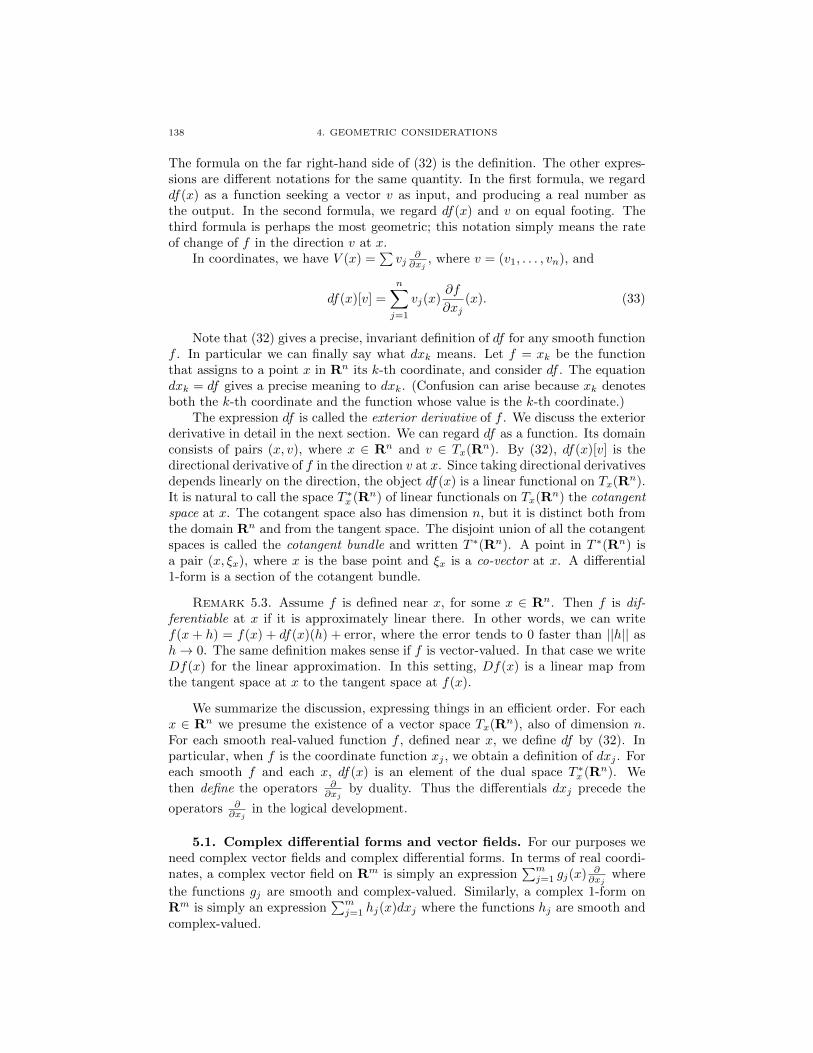
138 4. GEOMETRIC CONSIDERATIONS
The formula on the far right-hand side of (32) is the definition. The other expres-sions are different notations for the same quantity. In the first formula, we regarddf(x) as a function seeking a vector v as input, and producing a real number asthe output. In the second formula, we regard df(x) and v on equal footing. Thethird formula is perhaps the most geometric; this notation simply means the rateof change of f in the direction v at x.
In coordinates, we have V (x) =∑vj
∂∂xj
, where v = (v1, . . . , vn), and
df(x)[v] =
n∑j=1
vj(x)∂f
∂xj(x). (33)
Note that (32) gives a precise, invariant definition of df for any smooth functionf . In particular we can finally say what dxk means. Let f = xk be the functionthat assigns to a point x in Rn its k-th coordinate, and consider df . The equationdxk = df gives a precise meaning to dxk. (Confusion can arise because xk denotesboth the k-th coordinate and the function whose value is the k-th coordinate.)
The expression df is called the exterior derivative of f . We discuss the exteriorderivative in detail in the next section. We can regard df as a function. Its domainconsists of pairs (x, v), where x ∈ Rn and v ∈ Tx(Rn). By (32), df(x)[v] is thedirectional derivative of f in the direction v at x. Since taking directional derivativesdepends linearly on the direction, the object df(x) is a linear functional on Tx(Rn).It is natural to call the space T ∗x (Rn) of linear functionals on Tx(Rn) the cotangentspace at x. The cotangent space also has dimension n, but it is distinct both fromthe domain Rn and from the tangent space. The disjoint union of all the cotangentspaces is called the cotangent bundle and written T ∗(Rn). A point in T ∗(Rn) isa pair (x, ξx), where x is the base point and ξx is a co-vector at x. A differential1-form is a section of the cotangent bundle.
Remark 5.3. Assume f is defined near x, for some x ∈ Rn. Then f is dif-ferentiable at x if it is approximately linear there. In other words, we can writef(x + h) = f(x) + df(x)(h) + error, where the error tends to 0 faster than ||h|| ash→ 0. The same definition makes sense if f is vector-valued. In that case we writeDf(x) for the linear approximation. In this setting, Df(x) is a linear map fromthe tangent space at x to the tangent space at f(x).
We summarize the discussion, expressing things in an efficient order. For eachx ∈ Rn we presume the existence of a vector space Tx(Rn), also of dimension n.For each smooth real-valued function f , defined near x, we define df by (32). Inparticular, when f is the coordinate function xj , we obtain a definition of dxj . Foreach smooth f and each x, df(x) is an element of the dual space T ∗x (Rn). Wethen define the operators ∂
∂xjby duality. Thus the differentials dxj precede the
operators ∂∂xj
in the logical development.
5.1. Complex differential forms and vector fields. For our purposes weneed complex vector fields and complex differential forms. In terms of real coordi-nates, a complex vector field on Rm is simply an expression
∑mj=1 gj(x) ∂
∂xjwhere
the functions gj are smooth and complex-valued. Similarly, a complex 1-form onRm is simply an expression
∑mj=1 hj(x)dxj where the functions hj are smooth and
complex-valued.

5. VECTOR FIELDS AND DIFFERENTIAL FORMS 139
We can identify complex Euclidean space Cn with R2n. Write z = (z1, . . . , zn),and put zj = xj + iyj (where i is the imaginary unit). We can express vector fields
in terms of the ∂∂xj
and ∂∂yj
, and differential forms in terms of the dxj and dyj .
Complex geometry is magic, however. Things become much easier if we workdirectly with complex objects. Everything follows fairly easily from one obviousdefinition.
Definition 5.1. Suppose Ω is an open set in Cn, and f : Ω → C is smooth.Write f = u+ iv where u and v are real-valued. We define df by df = du+ idv.
Corollary 5.1. Let zj = xj + iyj denote the j-th coordinate function on Cn.Then dzj = dxj + idyj and dzj = dxj − idyj.
We define complex differentiation by duality as follows in Definition 5.2. Wecould also use the formulas in Corollary 5.2 as definitions.
Definition 5.2. For j = 1, . . . n, let ∂∂zj
, ∂∂zj denote the dual basis to the
basis dzj , dzj. Thus ∂∂zj
is defined by dzk[ ∂∂zj
] = 0 if j 6= k and by dzk[ ∂∂zk
] = 1.
Also, ∂∂zj
is defined by dzk[ ∂∂zj
] = 0 for all j, k and dzk[ ∂∂zj
] = 0 for j 6= k, but
dzk[ ∂∂zk
] = 1.
Differentiable functions g1, . . . , gm form a coordinate system on an open set Ωin Rm if their differentials are linearly independent on Ω and the mapping g =(g1, . . . , gm) is injective there. This concept makes sense when these functions areeither real or complex-valued. For example, the functions z and z can be regardedas (independent) coordinates on R2, because dx + idy and dx − idy are linearlyindependent and the map (x, y) → (x + iy, x − iy), embedding R2 into C2, isinjective.
We can regard the 2n functions z1, . . . , zn, z1, . . . , zn as complex-valued coor-dinates on R2n. The exterior derivative df is invariantly defined, independent ofcoordinate system, by (32) and Definition 5.1. Hence the following equality holds:
df =∑ ∂f
∂xjdxj +
∑ ∂f
∂yjdyj =
∑ ∂f
∂zjdzj +
∑ ∂f
∂zjdzj . (34)
The following formulas then follow by equating coefficients. See Exercise 5.1.
Corollary 5.2.∂
∂zj=
1
2
(∂
∂xj− i ∂
∂yj
)(35.1)
∂
∂zj=
1
2
(∂
∂xj+ i
∂
∂yj
). (35.2)
Suppose f is differentiable on an open set in Cn. We can then decompose itsexterior derivative df into two parts:
df = ∂f + ∂f =
n∑j=1
∂f
∂zjdzj +
n∑j=1
∂f
∂zjdzj . (36)
Definition 5.3. Let Ω be an open subset of Cn. Assume that f : Ω→ C andf is continuously differentiable. Then f is complex analytic if and only if ∂f
∂zj= 0
for all j. These equations are called the Cauchy-Riemann equations.

140 4. GEOMETRIC CONSIDERATIONS
As in one variable, complex analytic functions are given locally by convergentpower series. In Theorem 3.1 we used the power series expansion of a complexanalytic mapping in a ball. For most of what we do, the crucial point is that theCauchy-Riemann equations have the simple expression ∂f = 0.
Corollary 5.3. A continuously differentiable function, defined on an open setin Cn, is complex analytic if and only if df = ∂f .
In the rest of this chapter most of the complex analytic functions we will en-counter are polynomials. We emphasize the intuitive statement: f is complexanalytic if and only if f is independent of the conjugate variable z = (z1, . . . , zn).
Exercise 5.1. Verify (35.1) and (35.2). Start with (34) and equate coefficients.
Exercise 5.2. This exercise asks you to explain Remark 5.2. Consider thefunctions x and y as coordinates on R2. Then by definition, ∂y
∂x = 0. Supposeinstead we choose u = x and v = x + y as coordinates. Then we would have∂v∂u = 0. But ∂(x+y)
∂x = 1. Explain!
6. Differential forms of higher degree
Our work in higher dimensions relies on differential forms of higher degree. Thisdiscussion presumes that the reader has had some exposure to the wedge product ofdifferential forms, and therefore knows intuitively what we mean by a k-form. Wealso use the modern Stokes’ theorem, which in our setting expresses an integral of a2n-form over the unit ball as an integral of a (2n−1)-form over the unit sphere. Wesummarize enough of this material to enable us to do various volume computations.
Definition 6.1. Let V be a (real or) complex vector space of finite dimension.A function F : V × · · · × V → C (with k factors) is called a multi-linear form ifF is linear in each slot when the other variables are held fixed. We often say F isk-linear. It is called alternating if F (v1, . . . , vk) = 0 whenever vi = vj for some i, jwith i 6= j.
Example 6.1. Consider a k-by-k matrix M of (real or) complex numbers.Think of the rows (or columns) of M as elements of Ck. The determinant functionis an alternating k-linear form on Ck × · · · ×Ck.
Example 6.2. Given vectors a = (a1, a2, a3) and b = (b1, b2, b3) in R3, defineF (a, b) = a1b3 − a3b1. Then F is an alternating 2-linear form.
Lemma 6.1. A multi-linear form F (over Rn or Cn) is alternating if and onlyif the following holds. For each pair i, j of indices, the value of F is multiplied by−1 if we interchange the i-th and j-th slots:
F (v1, . . . , vi, . . . , vj , . . . vk) = −F (v1, . . . , vj , . . . vi, . . . , vk). (37)
Proof. It suffices to ignore all but two of the slots and then verify the resultwhen F is 2-linear. By multi-linearity we have
F (v + w, v + w) = F (v, v) + F (v, w) + F (w, v) + F (w,w). (38)
If F is alternating, then all terms in (38) vanish except F (v, w) + F (w, v). Hencethis term must vanish as well. Conversely, if this term always vanishes, then (38)gives F (v + w, v + w) = F (v, v) + F (w,w). Put w = −v. We get
0 = F (0, 0) = F (v, v) + F (−v,−v) = F (v, v) + (−1)2F (v, v) = 2F (v, v).
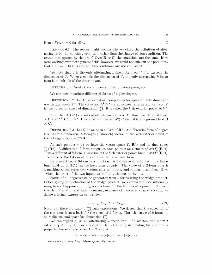
6. DIFFERENTIAL FORMS OF HIGHER DEGREE 141
Hence F (v, v) = 0 for all v.
Remark 6.1. The reader might wonder why we chose the definition of alter-nating to be the vanishing condition rather than the change of sign condition. Thereason is suggested by the proof. Over R or C, the conditions are the same. If wewere working over more general fields, however, we could not rule out the possibilitythat 1 + 1 = 0. In this case the two conditions are not equivalent.
We note that 0 is the only alternating k-linear form on V if k exceeds thedimension of V . When k equals the dimension of V , the only alternating k-linearform is a multiple of the determinant.
Exercise 6.1. Verify the statements in the previous paragraph.
We can now introduce differential forms of higher degree.
Definition 6.2. Let V be a (real or) complex vector space of finite dimensionn with dual space V ∗. The collection Λk(V ∗) of all k-linear alternating forms on Vis itself a vector space of dimension
(nk
). It is called the k-th exterior power of V ∗.
Note that Λ1(V ∗) consists of all 1-linear forms on V ; thus it is the dual spaceof V and Λ1(V ∗) = V ∗. By convention, we set Λ0(V ∗) equal to the ground field Ror C.
Definition 6.3. Let Ω be an open subset of Rn. A differential form of degreek on Ω (or a differential k-form) is a (smooth) section of the k-th exterior power ofthe cotangent bundle T ∗(Rn).
At each point x ∈ Ω we have the vector space Tx(Rn) and its dual spaceT ∗x (Rn). A differential k-form assigns to each point x an element of Λk(T ∗x (Rn)).Thus a differential k-form is a section of the k-th exterior power bundle Λk(T ∗(Rn)).The value of the k-form at x is an alternating k-linear form.
By convention, a 0-form is a function. A 1-form assigns to each x a linearfunctional on Tx(Rn), as we have seen already. The value of a 2-form at x isa machine which seeks two vectors at x as inputs, and returns a number. If weswitch the order of the two inputs we multiply the output by −1.
Forms of all degrees can be generated from 1-forms using the wedge product.Before giving the definition of the wedge product, we express the idea informallyusing bases. Suppose e1, . . . , en form a basis for the 1-forms at a point x. For eachk with 1 ≤ k ≤ n, and each increasing sequence of indices i1 < i2 < · · · < ik wedefine a formal expression eI , written
eI = ei1 ∧ ei2 ∧ · · · ∧ eik . (39)
Note that there are exactly(nk
)such expressions. We decree that the collection of
these objects form a basis for the space of k-forms. Thus the space of k-forms onan n-dimensional space has dimension
(nk
).
We can regard eI as an alternating k-linear form. As written, the index Isatisfies i1 < . . . ik. But we can extend the notation by demanding the alternatingproperty. For example, when k = 2 we put
(e1 ∧ e2)(v, w) = e1(v)e2(w)− e1(w)e2(v).
Then e2 ∧ e1 = −e1 ∧ e2. More generally we put
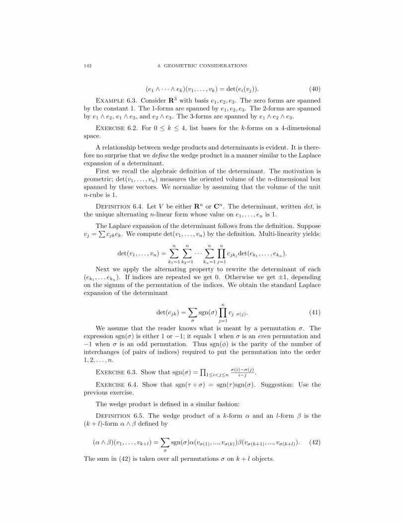
142 4. GEOMETRIC CONSIDERATIONS
(e1 ∧ · · · ∧ ek)(v1, . . . , vk) = det(ei(vj)). (40)
Example 6.3. Consider R3 with basis e1, e2, e3. The zero forms are spannedby the constant 1. The 1-forms are spanned by e1, e2, e3. The 2-forms are spannedby e1 ∧ e2, e1 ∧ e3, and e2 ∧ e3. The 3-forms are spanned by e1 ∧ e2 ∧ e3.
Exercise 6.2. For 0 ≤ k ≤ 4, list bases for the k-forms on a 4-dimensionalspace.
A relationship between wedge products and determinants is evident. It is there-fore no surprise that we define the wedge product in a manner similar to the Laplaceexpansion of a determinant.
First we recall the algebraic definition of the determinant. The motivation isgeometric; det(v1, . . . , vn) measures the oriented volume of the n-dimensional boxspanned by these vectors. We normalize by assuming that the volume of the unitn-cube is 1.
Definition 6.4. Let V be either Rn or Cn. The determinant, written det, isthe unique alternating n-linear form whose value on e1, . . . , en is 1.
The Laplace expansion of the determinant follows from the definition. Supposevj =
∑cjkek. We compute det(v1, . . . , vn) by the definition. Multi-linearity yields:
det(v1, . . . , vn) =
n∑k1=1
n∑k2=1
· · ·n∑
kn=1
n∏j=1
cjkjdet(ek1 , . . . , ekn).
Next we apply the alternating property to rewrite the determinant of each(ek1 , . . . ekn). If indices are repeated we get 0. Otherwise we get ±1, dependingon the signum of the permutation of the indices. We obtain the standard Laplaceexpansion of the determinant
det(cjk) =∑σ
sgn(σ)
n∏j=1
cj σ(j). (41)
We assume that the reader knows what is meant by a permutation σ. Theexpression sgn(σ) is either 1 or −1; it equals 1 when σ is an even permutation and−1 when σ is an odd permutation. Thus sgn(φ) is the parity of the number ofinterchanges (of pairs of indices) required to put the permutation into the order1, 2, . . . , n.
Exercise 6.3. Show that sgn(σ) =∏
1≤i<j≤nσ(i)−σ(j)
i−j .
Exercise 6.4. Show that sgn(τ σ) = sgn(τ)sgn(σ). Suggestion: Use theprevious exercise.
The wedge product is defined in a similar fashion:
Definition 6.5. The wedge product of a k-form α and an l-form β is the(k + l)-form α ∧ β defined by
(α ∧ β)(v1, . . . , vk+l) =∑σ
sgn(σ)α(vσ(1), ..., vσ(k))β(vσ(k+1), ..., vσ(k+l)). (42)
The sum in (42) is taken over all permutations σ on k + l objects.

6. DIFFERENTIAL FORMS OF HIGHER DEGREE 143
Proposition 6.1 (Properties of the wedge product). Let α and β be differentialforms. Then:
(1) α ∧ (β1 + β2) = (α ∧ β1) + (α ∧ β2).(2) α ∧ (β1 ∧ β2) = (α ∧ β1) ∧ β2.(3) α ∧ β = (−1)klβ ∧ α if α is a k-form and β is an l-form.
Proof. Left to the reader as Exercise 6.6.
The exterior derivative d is one of the most important and elegant operationsin mathematics. When η is a k-form, dη is a (k + 1)-form. When η is a function(a 0-form), dη agrees with our definition from (32). We extend d to forms of alldegrees.
One can define d by proceeding inductively on the degree of the form. If f is afunction, then df is defined as in (32) by df [v] = ∂f
∂v . In coordinates, df =∑ ∂f
∂xjdxj .
If g =∑j gjdxj is a 1-form, then
dg =∑j
dgj ∧ dxj =∑j
∑k
∂gj∂xk
dxk ∧ dxj =∑k<j
(∂gj∂xk− ∂gk∂xj
)dxk ∧ dxj . (43)
On the far right-hand side of (43), we have rewritten dg using dxk∧dxj = −dxj∧dxkto make the indices always increase. Of course the terms dxj ∧ dxj drop out. Forexample,
d(Pdx+Qdy) =∂P
∂ydy ∧ dx+
∂Q
∂xdx ∧ dy = (
∂Q
∂x− ∂P
∂y)dx ∧ dy. (44)
Let η be a k-form. We wish to define dη in coordinates. To simplify thenotation, write
dxJ = dxj1 ∧ dxj2 ∧ · · · ∧ dxjk .Then we can write η =
∑J ηJdx
J where the ηJ are functions and each J is ak-tuple of indices. We proceed as we did for 1-forms and put
dη =∑J
dηJ ∧ dxJ =∑J
∑k
∂ηJ∂xk
dxk ∧ dxJ .
Thus dη =∑gLdx
L, where now L is a (k + 1)-tuple of indices.The following standard result, which applies in the setting of smooth manifolds,
characterizes d. We omit the simple proof, which can be summarized as follows.Choose coordinates, use the properties to check the result in that coordinate system,and then use the chain rule to see that d is defined invariantly.
Theorem 6.1. There is a unique operator d mapping smooth k-forms to smooth(k + 1)-forms satisfying the following properties.
(1) If f is a function, then df is defined by (32).(2) d(α+ β) = dα+ dβ.(3) d(α ∧ β) = dα ∧ β + (−1)kα ∧ dβ if α is a k-form.(4) d2 = 0.
It is possible to define d without resorting to a coordinate system. The definitionon 0-forms is as in (32). We give the definition only for 1-forms. Let η be a 1-form;the 2-form dη requires two vector fields as inputs; it must be alternating and multi-linear. Thus we will define dη(v, w) for vector fields v and w.
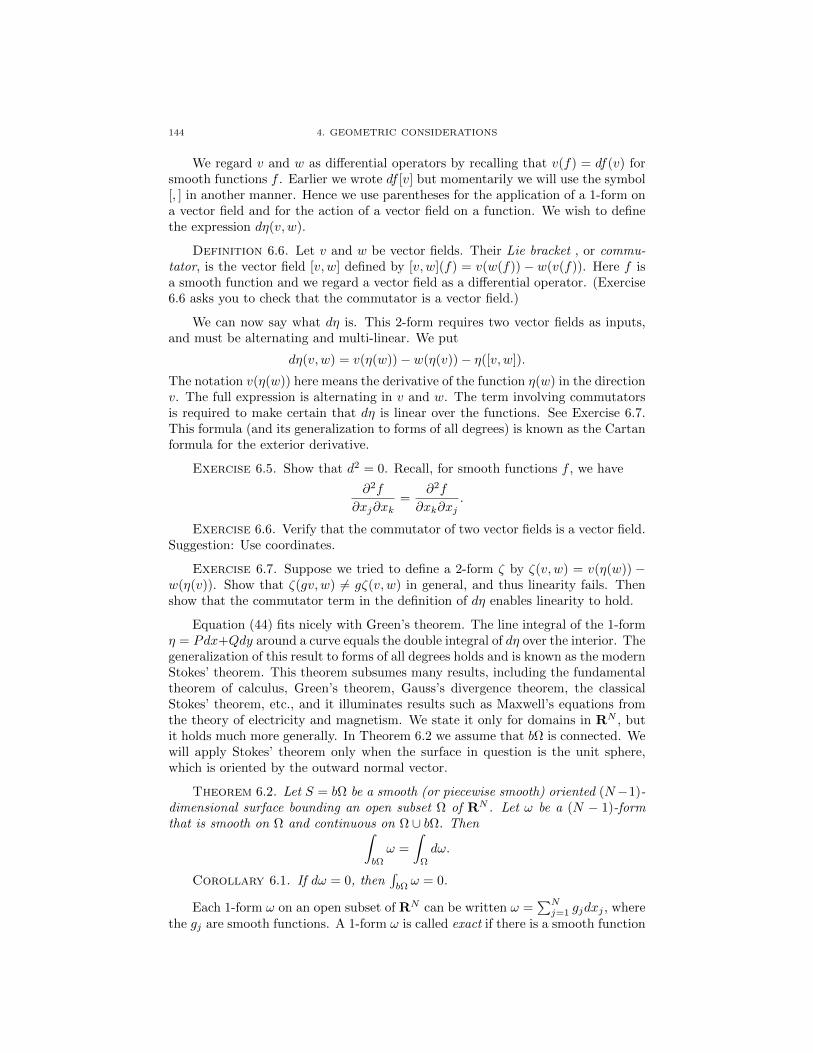
144 4. GEOMETRIC CONSIDERATIONS
We regard v and w as differential operators by recalling that v(f) = df(v) forsmooth functions f . Earlier we wrote df [v] but momentarily we will use the symbol[, ] in another manner. Hence we use parentheses for the application of a 1-form ona vector field and for the action of a vector field on a function. We wish to definethe expression dη(v, w).
Definition 6.6. Let v and w be vector fields. Their Lie bracket , or commu-tator, is the vector field [v, w] defined by [v, w](f) = v(w(f))− w(v(f)). Here f isa smooth function and we regard a vector field as a differential operator. (Exercise6.6 asks you to check that the commutator is a vector field.)
We can now say what dη is. This 2-form requires two vector fields as inputs,and must be alternating and multi-linear. We put
dη(v, w) = v(η(w))− w(η(v))− η([v, w]).
The notation v(η(w)) here means the derivative of the function η(w) in the directionv. The full expression is alternating in v and w. The term involving commutatorsis required to make certain that dη is linear over the functions. See Exercise 6.7.This formula (and its generalization to forms of all degrees) is known as the Cartanformula for the exterior derivative.
Exercise 6.5. Show that d2 = 0. Recall, for smooth functions f , we have
∂2f
∂xj∂xk=
∂2f
∂xk∂xj.
Exercise 6.6. Verify that the commutator of two vector fields is a vector field.Suggestion: Use coordinates.
Exercise 6.7. Suppose we tried to define a 2-form ζ by ζ(v, w) = v(η(w)) −w(η(v)). Show that ζ(gv, w) 6= gζ(v, w) in general, and thus linearity fails. Thenshow that the commutator term in the definition of dη enables linearity to hold.
Equation (44) fits nicely with Green’s theorem. The line integral of the 1-formη = Pdx+Qdy around a curve equals the double integral of dη over the interior. Thegeneralization of this result to forms of all degrees holds and is known as the modernStokes’ theorem. This theorem subsumes many results, including the fundamentaltheorem of calculus, Green’s theorem, Gauss’s divergence theorem, the classicalStokes’ theorem, etc., and it illuminates results such as Maxwell’s equations fromthe theory of electricity and magnetism. We state it only for domains in RN , butit holds much more generally. In Theorem 6.2 we assume that bΩ is connected. Wewill apply Stokes’ theorem only when the surface in question is the unit sphere,which is oriented by the outward normal vector.
Theorem 6.2. Let S = bΩ be a smooth (or piecewise smooth) oriented (N−1)-dimensional surface bounding an open subset Ω of RN . Let ω be a (N − 1)-formthat is smooth on Ω and continuous on Ω ∪ bΩ. Then∫
bΩ
ω =
∫Ω
dω.
Corollary 6.1. If dω = 0, then∫bΩω = 0.
Each 1-form ω on an open subset of RN can be written ω =∑Nj=1 gjdxj , where
the gj are smooth functions. A 1-form ω is called exact if there is a smooth function
7. VOLUMES OF PARAMETRIZED SETS 145
f such that ω = df ; thus gj = ∂f∂xj
. Readers who are familiar with regarding
line integrals as computing work will recognize that exact forms correspond toconservative force fields. A necessary condition for being exact arises in calculus.A form η is called closed if dη = 0. The reader certainly knows that exact impliesclosed (a consequence of d2 = 0), but closed on an open set does not imply exactthere. The standard example is of course
ω =−ydx+ xdy
x2 + y2(45)
on the complement of the origin in R2. The form in (45) leads to the subject ofdeRham cohomology. One relates the existence and number of holes in a space towhether closed forms are exact.
Exercise 6.8. Prove Proposition 6.1.
Exercise 6.9. For 0 < r <∞ and 0 ≤ θ < 2π, put (x, y) = (rcos(θ), rsin(θ)).Show that dx ∧ dy = rdr ∧ dθ.
Exercise 6.10. For 0 < ρ <∞, for 0 ≤ θ < 2π, and for 0 ≤ φ < π, put
(x, y, z) = (ρcos(θ)sin(φ), ρsin(θ)sin(φ), ρcos(φ)).
Compute dx ∧ dy ∧ dz in terms of ρ, θ, φ, dρ, dθ, dφ.
Exercise 6.11. Express the complex 1-form dzz in terms of x, y, dx, dy. Express
the form in (45) in terms of dz and dz.
Exercise 6.12. Show that dz ∧ dz = −2idx ∧ dy.
Exercise 6.13. Put z = reiθ. Compute dz ∧ dz.
Exercise 6.14. Put ω = dx1 ∧ dx2 + dx3 ∧ dx4. Find ω ∧ ω. The answer isnot 0. Explain.
Exercise 6.15. For n ≥ 3, what is the analogue of (45) for the complement ofthe origin in Rn?
Exercise 6.16. Use wedge products to give a test for deciding whether acollection of 1-forms is linearly independent.
Exercise 6.17. For n ≥ k ≥ 2, let r1, . . . rk be smooth real-valued functionson Cn. Show that it is possible for dr1, . . . , drk to be linearly independent while∂r1, . . . , ∂rk are linearly dependent. Here ∂r =
∑∂r∂zj
dzj . This problem is even
easier if we drop the assumption that the rj are real-valued. Why?
7. Volumes of parametrized sets
Our next geometric inequality extends the ideas of Proposition 1.1 to higherdimensions. Things are more complicated for several reasons, but we obtain a sharpinequality on volumes of images of proper polynomial mappings between balls. Wewill also need some computations from multi-variable calculus which are useful inmany contexts.
We begin with a quick review of higher dimensional volume. Let Ω be an opensubset of Rk. Let u1, . . . , uk be coordinates on Rk. Suppose F : Ω → RN iscontinuously differentiable and injective, except perhaps on a small set. Let us alsoassume that the derivative map DF : Rk → RN is injective, again except perhaps

146 4. GEOMETRIC CONSIDERATIONS
on a small set. At each x, DF (x) is a linear map from Tx(Rk)→ TF (x)(RN ). Let
(DF )(x)∗ denote the transpose of DF (x). Then (DF )(x)∗ : TF (x)(RN )→ Tx(Rk).
The composition (DF )∗(x)DF (x) is then a linear mapping of the space Tx(Rk) toitself, and hence its determinant is defined. Then the k-dimensional volume of theset F (Ω) is given by an integral:
Vol(F (Ω)) =
∫Ω
√det((DF )∗DF )du1 ∧ · · · ∧ duk. (46)
In (46), the ordering of the duj defines the orientation on Rk. We sometimes writedVk or dVk(u) instead of du1 ∧ · · · ∧ duk for the Euclidean volume form.
Example 7.1. Let Ω denote the unit disk in R2 with coordinates x, y. Wedefine a family of maps Fα : Ω→ R4 by
Fα(x, y) = (cos(α)x, cos(α)y, sin(α)(x2 − y2), sin(α)2xy).
Computation shows that
DFα =
cos(α) 0
0 cos(α)2xsin(α) −2ysin(α)2ysin(α) 2xsin(α)
. (47)
Matrix multiplication shows that DF ∗α(x)DFα(x) is the matrix in (48):(cos2(α) + 4(x2 + y2)sin2(α) 0
0 cos2(α) + 4(x2 + y2)sin2(α)
). (48)
Hence√
det(DF ∗αDFα) = cos2(α) + 4(x2 + y2)sin2(α). Thus the area of the imageof the unit disk B1 under Fα is the integral:∫
B1
(cos2(α) + 4(x2 + y2)sin2(α))dxdy = π(1 + sin2(α)). (49)
Example 7.2. As both an example and to anticipate a later development, wefind the 3-dimensional volume of S3. We write s =
√1− r2. Define a map F on
the open set 0 < r < 1, 0 < θ < 2π, 0 < φ < 2π by
(r, θ, φ)→ F (r, θ, φ) = (r cos(θ), r sin(θ), s cos(φ), s sin(φ))
Computing DF and DF ∗ gives
(DF )∗ =
cos(θ) sin(θ) −rs2 cos(φ) −r
s2 sin(φ)−r sin(θ) r cos(θ) 0 0
0 0 −s sinφ s cos(φ).
Multiplying (DF )∗ by DF and computing determinants yields the 3-dimensionalvolume form rdrdθdφ on the sphere. Thus
Vol(S3) =
∫ 2π
0
∫ 2π
0
∫ 1
0
rdrdθdφ = (2π)2 1
2= 2π2.
We are primarily interested in images of sets in Cn under complex analyticmappings. When f is a complex-analytic and equi-dimensional mapping, we writef ′ for its derivative and Jf for its Jacobian determinant. Thus
Jf = det
(∂fj∂zk
).

7. VOLUMES OF PARAMETRIZED SETS 147
Volume computations simplify in the complex-analytic case, even when f is notequi-dimensional. For example, we could express Example 7.1 using the complexanalytic map fα defined by fα(z) = (cos(α)z, sin(α)z2) and we easily obtain (49).Part of the explanation comes from the following result in the equi-dimensionalcase.
Lemma 7.1. Suppose f : Ω ⊂ Cn → Cn is complex analytic. Define F : R2n →R2n by F (x, y) = (Re(f(x+iy)), Im(f(x+iy)). Then det(DF ) = |det(f ′)|2 = |Jf |2.
Proof. We know that det(DF ) is the factor required in the volume formwhen we change variables. Thus, if u = F (x), then dV (u) = det((DF )(x))dV (x).The proof amounts to rewriting this equality using complex variables and theirconjugates, and using the relationship between wedge products and determinants.
Put w = f(z), where both z and w are in Cn. Put w = u+ iv and z = x+ iy.In real variables we have
dV2n(u, v) = du1∧dv1∧· · ·∧dun∧dvn = det(DF )dx1∧dy1∧· · ·∧dxn∧dyn. (50)
We will write the volume forms in the z, z variables in the domain and the w,wvariables in the target. Note that
dwj =∑ ∂fj
∂zkdzk.
Hence dw1 ∧ · · · ∧ dwn = det(∂fj∂zk
)dz1 ∧ · · · ∧ dzn = det(Jf)dz1 ∧ · · · ∧ dzn.
Recall from Exercise 6.12 that dzj ∧ dzj = (−2i)dxj ∧ dyj and similarly for thew variables. Putting everything together we get
dV2n(u, v) = du1 ∧ dv1 ∧ · · · ∧ dun ∧ dvn = (i
2)ndw1 ∧ dw1 ∧ · · · ∧ dwn ∧ dwn
= |det(f ′(z))|2(i
2)ndz1 ∧ dz1 ∧ · · · ∧ dzn ∧ dzn
= |det(f ′(z))|2dx1 ∧ dy1 ∧ · · · ∧ dxn ∧ dyn = |det(f ′(z))|2dV2n(x, y). (51)
Comparing (50) and (51) finishes the proof.
Exercise 7.1. Prove (51) using the Cauchy-Riemann equations. The compu-tation is somewhat punishing; do it only in two complex variables where you willdeal with four-by-four matrices.
We continue discussing higher dimensional volumes of complex analytic images.Let ω denote the differential form on CN defined by
ω =i
2
N∑j=1
dζj ∧ dζj .
The factor i2 arises because dz ∧ dz = −2idx ∧ dy in one dimension. See Exercise
6.12. The form ωk, where we wedge ω with itself k times, is used to define 2k-dimensional volume. As before we take multiplicity into account.
Definition 7.1. (2k-dimensional volume) Let Ω be an open subset in Ck, andsuppose that f : Ω → CN is complex analytic. We define V2k(f,Ω), the (2k)-dimensional volume with multiplicity counted, by (52):

148 4. GEOMETRIC CONSIDERATIONS
V2k(f,Ω) =
∫Ω
(f∗ω)k
k!=
1
k!
∫Ω
(i
2)k(
N∑j=1
∂fj ∧ ∂fj)k. (52)
Remark 7.1. Equation (52) is the natural definition based on our L2 perspec-tive. When f is not injective, the formula takes multiplicity into account. Forw ∈ CN , let #(f, w) denote the number of points in Ω ∩ f−1(w). Then we coulddefine V2k(f,Ω) by
V2k(f,Ω) =
∫CN
#(f, w)dh2k(w).
Here dh2k(w) is the 2k-dimensional Hausdorff measure. The so-called area formulafrom Geometric Measure Theory shows under rather general hypotheses, met inour context, that this computation agrees with (52).
We are primarily interested in the case when Ω is the unit ball Bk; in this casewe abbreviate V2k(f,Ω) by Vf . In (52) the upper star notation denotes pullback,and the k! arises because there are k! ways to permute the indices from 1 to k. The
form (f∗ω)k
k! is rdV , where dV = dV2k is the Euclidean volume form in k complexdimensions, for some function r depending on f . In the next section we providetechniques for evaluating the resulting integrals.
Example 7.3. We consider several maps from B2 to C3. Using (52) and themethods of the next section we obtain the following values:
(1) Put g(z, w) = (z, 0, w). Then Vg = π2
2 .
(2) For 0 ≤ λ ≤√
2, put f(z, w) = (z2, λzw,w2). Then Vf = 2(λ2+1)3 π2.
The first map is injective, and Vf gives the volume of the image. For λ 6= 0, thesecond map is generically two-to-one. If (a, b, c) is in the image of f , and (a, b, c) isnot the origin, then f−1(a, b, c) has precisely two points. When λ2 = 2, we obtain4 times the volume of the unit ball. See Theorem 8.1. When λ = 0, the answer is43 times the volume of the unit ball.
Example 7.4. Define h : C2 → C3 by h(z, w) = (z, zw,w2). This map and itsgeneralization to higher dimensions will play an important role for us, because hmaps the unit sphere in C2 into the unit sphere in C3. We use it here to illustratethe subtleties involved in computing multiplicities. Let p = (a, b, c) be a point inC3. Suppose first that a 6= 0. Then h−1(p) is empty unless b2 = ca2, in whichcase h−1(p) is a single point. When a = 0, things change. If b 6= 0, then h−1(p)is empty. If a = b = 0, then h−1(p) consists of two points for c 6= 0 and one pointwith multiplicity two if c = 0.
For us, the easiest method of computation will use the expanded version of thefar right-hand side of (53). We explain why. Let Ω be an open set in Ck, andassume that f : Ω→ CN is complex analytic. Here we allow the target dimensionto differ from the domain dimension. We define the pointwise squared Jacobian||Jf ||2 by
||Jf ||2 =∑|J(fi1 , ..., fik)|2 =
∑|J(fI)|2. (53)
The sum in (53) is taken over all increasing k-tuples. Equivalently, we form allpossible Jacobian determinants of k of the component functions, and sum their

8. VOLUME COMPUTATIONS 149
squared moduli. Recall, in the equi-dimensional case, that
Jg = det
(∂gj∂zk
).
Exercise 7.2. Let α =∑4j=1 ∂fj ∧∂fj Find α∧α∧α by expanding. Compare
with (53).
The next Lemma provides another method for finding Vf . When consideredwith Lemma 7.1, we see why L2 considerations arise.
The complex Hessian Hr of a twice differentiable function r of several com-
plex variables is the matrix(
∂2r∂zj∂zk
). The following result relates the Hessian to
Jacobian determinants when r = ||f ||2 is a squared norm of a complex analyticmapping.
Lemma 7.2. If f : Ck → CN is complex analytic, then ||Jf ||2 = det(H(||f ||2)).
Proof. See Exercise 7.3.
Thus finding the volume (with multiplicity accounted for) of the image of acomplex analytic mapping f : Ω ⊂ Ck → CN involves L2 norms. We must sumthe L2 norms of each Jacobian J(fj1 , ..., fjk) formed from the components of f :
V2k(f,Ω) =
∫Ω
||Jf ||2dV2k =
∫Ω
H(||f ||2)dV2k. (54)
Exercise 7.3. Put r(z, z) =∑Nj=1 |fj(z)|2 = ||f(z)||2. Use differential forms
to prove Lemma 7.2.
8. Volume computations
Our next goal is to compute the 2n-dimensional volume of the image of theunit ball in Cn under the mapping z 7→ z⊗m. As a warm-up, suppose n = 1. Thenthe map z 7→ zm covers the ball m times, and hence the area of the image withmultiplicity counted is πm. We get the same answer using integrals:
A =
∫B1
|mzm−1|2dV = m2
∫ 2π
0
∫ 1
0
r2m−1drdθ = m2 2π
2m= πm. (55)
In order to help us do computations and to simplify the notation, we brieflydiscuss multi-index notation. Let α = (α1, . . . , αn) be an n-tuple of non-negativenumbers, not necessarily integers. We call α a multi-index. When the αj areintegers we write |α| =
∑nj=1 αj and α! =
∏nj=1 αj !. In case d = |α|, we write
multinomial coefficients using multi-indices:(d
α
)=d!
α!=
d!
α1! . . . αn!.
Multi-indices are especially useful for writing polynomials and power series. Ifz ∈ Cn, we write
zα =
n∏j=1
(zj)αj
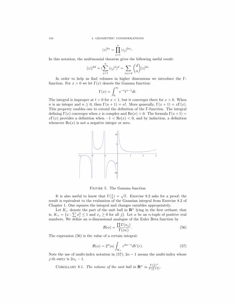
150 4. GEOMETRIC CONSIDERATIONS
|z|2α =
n∏j=1
|zj |2αj .
In this notation, the multinomial theorem gives the following useful result:
||z||2d = (
n∑j=1
|zj |2)d =∑|α|=d
(d
α
)|z|2α
In order to help us find volumes in higher dimensions we introduce the Γ-function. For x > 0 we let Γ(x) denote the Gamma function:
Γ(x) =
∫ ∞0
e−ttx−1dt.
The integral is improper at t = 0 for x < 1, but it converges there for x > 0. Whenn is an integer and n ≥ 0, then Γ(n + 1) = n!. More generally, Γ(x + 1) = xΓ(x).This property enables one to extend the definition of the Γ-function. The integraldefining Γ(x) converges when x is complex and Re(x) > 0. The formula Γ(x+ 1) =xΓ(x) provides a definition when −1 < Re(x) < 0, and by induction, a definitionwhenever Re(x) is not a negative integer or zero.
-3 -2 -1 1 2 3
-10
-5
5
10
Figure 5. The Gamma function
It is also useful to know that Γ( 12 ) =
√π. Exercise 8.2 asks for a proof; the
result is equivalent to the evaluation of the Gaussian integral from Exercise 8.2 ofChapter 1. One squares the integral and changes variables appropriately.
Let K+ denote the part of the unit ball in Rn lying in the first orthant; thatis, K+ = x :
∑x2j ≤ 1 and xj ≥ 0 for all j. Let α be an n-tuple of positive real
numbers. We define an n-dimensional analogue of the Euler Beta function by
B(α) =
∏Γ(αj)
Γ(|α|). (56)
The expression (56) is the value of a certain integral:
B(α) = 2n|α|∫K+
r2α−1dV (r). (57)
Note the use of multi-index notation in (57); 2α − 1 means the multi-index whosej-th entry is 2αj − 1.
Corollary 8.1. The volume of the unit ball in Rn isΓ( 1
2 )n
Γ(n2 +1) .

8. VOLUME COMPUTATIONS 151
Proof. Put α = ( 12 ,
12 , ...,
12 ) in (56) and use (57).
Exercise 8.1. Verify that Γ(x+ 1) = xΓ(x) and Γ(n+ 1) = n!.
Exercise 8.2. Show that Γ( 12 ) =
√π.
Exercise 8.3. Express the formula for the volume of the unit ball in Rn inthe form cnπ
n. (Use the previous exercise.)
Exercise 8.4. Put β(a, b) =∫ 1
0ta−1(1 − t)b−1dt for a, b > 0. This integral is
the classical Euler Beta function. Evaluate it in terms of the Γ-function. Explainthe relationship with (57).
Exercise 8.5. Prove that (56) and (57) are equivalent.
Remark 8.1. Integrals of the form∫ 2π
0cosk(θ)sinl(θ)dθ (for integer exponents)
are easily evaluated by using the complex form of the exponential. Integrals of the
form∫ π
2
0cosk(θ)sinl(θ)dθ are harder. Such integrals reduce to Beta functions:
β(a, b) =
∫ 1
0
ta−1(1− t)b−1dt = 2
∫ π2
0
sin2a−1(θ)cos2b−1(θ)dθ
even when a and b are not integers.
Exercise 8.6. Use the Euler-Beta function to verify the following duplicationformula for the Γ function.
Γ(x)
Γ(2x)= 21−2x Γ( 1
2 )
Γ(x+ 12 ). (58)
Suggestion. First multiply both sides by Γ(x). The left-hand side of the result isthen β(x, x). Write it as a single integral over [0, 1] as in Exercise 8.4. Rewrite bysymmetry as twice the integral over [0, 1
2 ]. Then change variables by 2t = 1−√s.
You will obtain 21−2xβ(x, 12 ) and (58) follows.
Exercise 8.7. Put φ(x, y) = Γ(x)Γ(x+y)Γ(2x)Γ(y) . Find φ(x, 1
2 ) and φ(x, 32 ). Show that
φ(x,5
2) = 21−2x (1 + 2x)(3 + 2x)
3.
Exercise 8.8. (Difficult) Verify the following formula for Γ(z)Γ(1− z):
Γ(z)Γ(1− z) =π
sin(πz).
Suggestion: First obtain a Beta function integral. Convert it to an integral over[0,∞). Then use contour integration. The computation is valid for all complexnumbers except the integers. See also Exercise 11.4 of Chapter 3.
The following exercise gives another circumstance in which the Γ function arisesnaturally.
Exercise 8.9. (For those who know probability). Let X be a Gaussian randomvariable with mean 0 and variance σ2. Use the fundamental theorem of calculusto find the density of the random variable X2. The answer is called the Γ-densitywith parameters 1
2 and 12σ2 . Use this method to show that Γ( 1
2 ) =√π.
We will evaluate several integrals using the n-dimensional Beta function.

152 4. GEOMETRIC CONSIDERATIONS
Lemma 8.1. Let d be a non-negative integer, and let α be a multi-index ofnon-negative real numbers. Let Bn denote the unit ball in Cn. Then∫
Bn
||z||2ddV =πn
(n− 1)!(n+ d). (59.1)∫
Bn
|z|2αdV =πn
(n+ |α|)B(α+ 1). (59.2)
Proof. We use polar coordinates in each variable separately; to evaluate (59.1)we have
I =
∫Bn
||z||2ddV2n = (2π)n∫K+
||r||2d∏
rjdVn.
We then expand ||r||2d using the multinomial theorem to obtain (60):
I = πn2n∑|γ|=d
(d
γ
)∫K+
r2γ+1dVn. (60)
Using formulas (56) and (57) for the Beta function in (60) we obtain
I = πn∑|γ|=d
(d
γ
)B(γ + 1)
|γ + 1|= πn
∑|γ|=d
d!∏γj
∏γj
(d+ n)Γ(d+ n)= πn
d!
(d+ n)!
∑|γ|=d
1.
(61)By Exercise 4.4, the number of independent homogeneous monomials of degree
d in n variables is(n+d−1
d
). We replace the sum in the last term in (61) with this
number to obtain the desired result:
I = πnd!
(d+ n)!
(n+ d− 1)!
(n− 1)!d!=
πn
(n− 1)!(n+ d). (62)
The calculation of (59.2) is similar but easier as there is no summation to compute:
I =
∫Bn
|z|2αdV2n = (2π)n∫K+
r2α+1dVn = πnB(α+ 1)
|α|+ n.
For convenience we write (59.2) when n = 2 and a, b are integers:∫B2
|z|2a|w|2bdV4 =π2a!b!
(a+ b+ 2)!. (63)
We offer one piece of caution. In the complex 2-dimensional case, the volume formis rdV4, where r = EG− |F |2, and we have:
E = ||∂f∂z||2,
G = || ∂f∂w||2,
F = 〈∂f∂z,∂f
∂w〉. (64)
8. VOLUME COMPUTATIONS 153
There is no square root here; by contrast, the classical formula for the surface areaform in the real case is
√EG− F 2, where E,G, F have definitions analogous to
(64).
We return to the homogeneous mapping Hm(z). We consider Hm : Bk → CN ,
where N =(k+m−1k−1
), the dimension of the space of homogeneous polynomials of
degree m in k variables. We use the following lemma to find (Theorem 8.1) anexplicit formula for the 2k-dimensional volume (with multiplicity counted) of theimage of the unit ball under Hm.
Lemma 8.2. The pullback k-th power (H∗m(ω))k satisfies the following:
(H∗m(ω))k = mk+1k!||z||2k(m−1)dV2k. (65)
Proof. Note first that (H∗m(ω))k is a smooth (2k)-form, and hence a multipler of dV2k. Note next that Hm is invariant under unitary transformations, andtherefore r must be a function of ||z||2. Since Hm is homogeneous of degree m, eachfirst derivative is homogeneous of degree m− 1. The (1, 1) form H∗m(ω) must thenhave coefficients that are bihomogeneous of degree (m− 1,m− 1). The coefficientr of its k-th power must be homogeneous of degree 2k(m − 1). Combining thehomogeneity with the dependence on ||z||2 gives the desired expression, except forevaluating the constant mk+1k!.
For simplicity we write |dzj |2 for dzj ∧ dzj . To evaluate the constant it suffices
to compute the coefficient of |z1|2k(m−1). To do so, we compute dHm, and thenwork modulo z2, ..., zn. Thus, in the formula for (H∗m(ω))k we set all variables equalto zero except the first. Doing so yields
H∗m(ω) = m2|z1|2m−2|dz1|2 +m|z1|2m−2k∑j=2
|dzj |2. (66)
From (66) it suffices to compute
(m2|dz1|2 +m
k∑j=2
|dzj |2)k. (67)
Expanding (67) yields
k!mk+1dz1 ∧ dz1 ∧ ... ∧ dzk ∧ dzk,and (65) follows by putting the factor |z1|(2m−2)k from (66) back in.
Theorem 8.1. Let f : Bn → BK be a proper complex analytic homogeneouspolynomial mapping of degree m. The 2n-dimensional volume Vf (with multiplicitycounted) is given by
Vf = mnπn1
n!. (68)
Proof. Consider the function ||f ||2. Since
||f(z)||2 = 1 = ||z||2m = ||Hm(z)||2
on the unit sphere, and both f and Hm are homogeneous, this equality holdseverywhere. Hence ||f ||2 = ||Hm||2 and these two functions have the same complexHessian determinant. By Lemma 8.2 they determine the same volume form:
154 4. GEOMETRIC CONSIDERATIONS
∑I
|J(fI)|2 =∑I
|J((Hm)I))|2,
and hence by Lemma 8.2
Vf =
∫Bn
(H∗m(ω))n
n!=
∫Bn
mn+1||z||2n(m−1)dV2n.
Lemma 8.1 yields
Vf = mn+1 πn
(n(m− 1) + n)
1
(n− 1)!=mnπn
n!.
As a check we observe, when m = 1, that Vf = πn
n! , which is the volume of Bn.When n = 1, we obtain Vf = πm, which is also the correct result, as we observedin (55).
The factor of mn arising in (68) arises because the image of the unit sphere inCn covers m times a subset of the unit sphere in the target. Compare with item(2) of Example 7.3.
9. Inequalities
We are at last ready to state a sharp inequality.
Theorem 9.1. Let p : Cn → CN be a polynomial mapping of degree m. Assumethat p(S2n−1) ⊂ S2N−1. Then Vp ≤ mnπn
n! . Equality happens if and only if p ishomogeneous of degree m.
Proof. If p is homogeneous of degree m, the result is Theorem 8.1. If not, thenwe apply the process from Theorem 4.3 until we obtain a homogeneous mapping.The key point is that the operation of tensoring with z on a subspace A alwaysincreases the volume of the image, in analogy with Proposition 1.1.
The key point is equivalent to the following statement, which we state andprove as Theorem 9.2 below. Put f = (f1, . . . , fN ). Put
g = (z1f1, . . . , znf1, f2, . . . , fN ). (69)
Then Vf ≤ Vg, with equality only if f1 = 0. Therefore, each tensor operationfrom Theorem 4.3 increases the integral. We stop when we reach a homogeneousmap.
With g as in (69), we need to verify that Vf ≤ Vg. We proved this result(Corollary 1.2) when n = N = 1, in two ways. One can prove the general resultin both fashions, but the computations are more elaborate. We give the geometricproof involving a boundary integral.
Theorem 9.2. Assume that f = (f1, ..., fN ) is complex analytic on the unitball Bn in Cn. Define the partial tensor product Ef by
Ef = (z1f1, z2f1, . . . , znf1, f2, . . . , fN ). (70)
Then VEf > Vf unless f1 = 0.
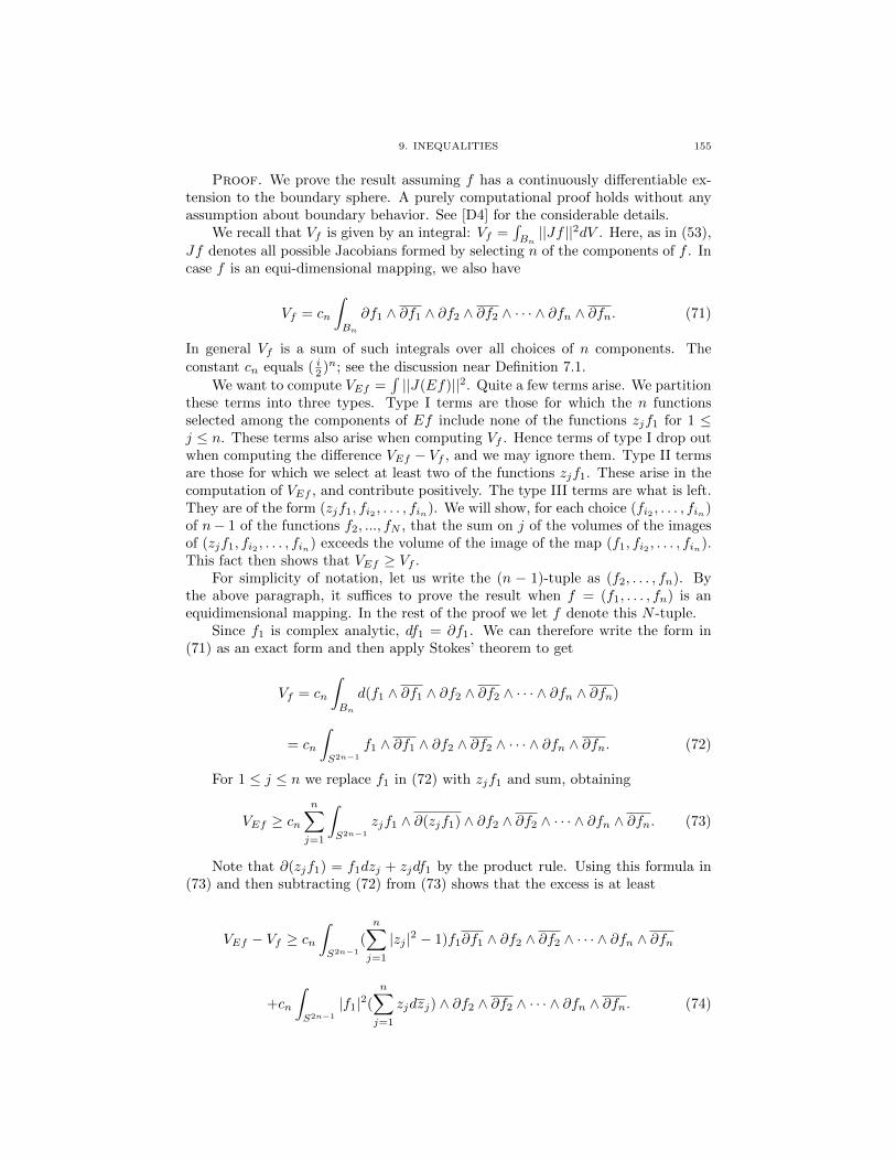
9. INEQUALITIES 155
Proof. We prove the result assuming f has a continuously differentiable ex-tension to the boundary sphere. A purely computational proof holds without anyassumption about boundary behavior. See [D4] for the considerable details.
We recall that Vf is given by an integral: Vf =∫Bn||Jf ||2dV . Here, as in (53),
Jf denotes all possible Jacobians formed by selecting n of the components of f . Incase f is an equi-dimensional mapping, we also have
Vf = cn
∫Bn
∂f1 ∧ ∂f1 ∧ ∂f2 ∧ ∂f2 ∧ · · · ∧ ∂fn ∧ ∂fn. (71)
In general Vf is a sum of such integrals over all choices of n components. Theconstant cn equals ( i2 )n; see the discussion near Definition 7.1.
We want to compute VEf =∫||J(Ef)||2. Quite a few terms arise. We partition
these terms into three types. Type I terms are those for which the n functionsselected among the components of Ef include none of the functions zjf1 for 1 ≤j ≤ n. These terms also arise when computing Vf . Hence terms of type I drop outwhen computing the difference VEf − Vf , and we may ignore them. Type II termsare those for which we select at least two of the functions zjf1. These arise in thecomputation of VEf , and contribute positively. The type III terms are what is left.They are of the form (zjf1, fi2 , . . . , fin). We will show, for each choice (fi2 , . . . , fin)of n− 1 of the functions f2, ..., fN , that the sum on j of the volumes of the imagesof (zjf1, fi2 , . . . , fin) exceeds the volume of the image of the map (f1, fi2 , . . . , fin).This fact then shows that VEf ≥ Vf .
For simplicity of notation, let us write the (n − 1)-tuple as (f2, . . . , fn). Bythe above paragraph, it suffices to prove the result when f = (f1, . . . , fn) is anequidimensional mapping. In the rest of the proof we let f denote this N -tuple.
Since f1 is complex analytic, df1 = ∂f1. We can therefore write the form in(71) as an exact form and then apply Stokes’ theorem to get
Vf = cn
∫Bn
d(f1 ∧ ∂f1 ∧ ∂f2 ∧ ∂f2 ∧ · · · ∧ ∂fn ∧ ∂fn)
= cn
∫S2n−1
f1 ∧ ∂f1 ∧ ∂f2 ∧ ∂f2 ∧ · · · ∧ ∂fn ∧ ∂fn. (72)
For 1 ≤ j ≤ n we replace f1 in (72) with zjf1 and sum, obtaining
VEf ≥ cnn∑j=1
∫S2n−1
zjf1 ∧ ∂(zjf1) ∧ ∂f2 ∧ ∂f2 ∧ · · · ∧ ∂fn ∧ ∂fn. (73)
Note that ∂(zjf1) = f1dzj + zjdf1 by the product rule. Using this formula in(73) and then subtracting (72) from (73) shows that the excess is at least
VEf − Vf ≥ cn∫S2n−1
(
n∑j=1
|zj |2 − 1)f1∂f1 ∧ ∂f2 ∧ ∂f2 ∧ · · · ∧ ∂fn ∧ ∂fn
+cn
∫S2n−1
|f1|2(
n∑j=1
zjdzj) ∧ ∂f2 ∧ ∂f2 ∧ · · · ∧ ∂fn ∧ ∂fn. (74)
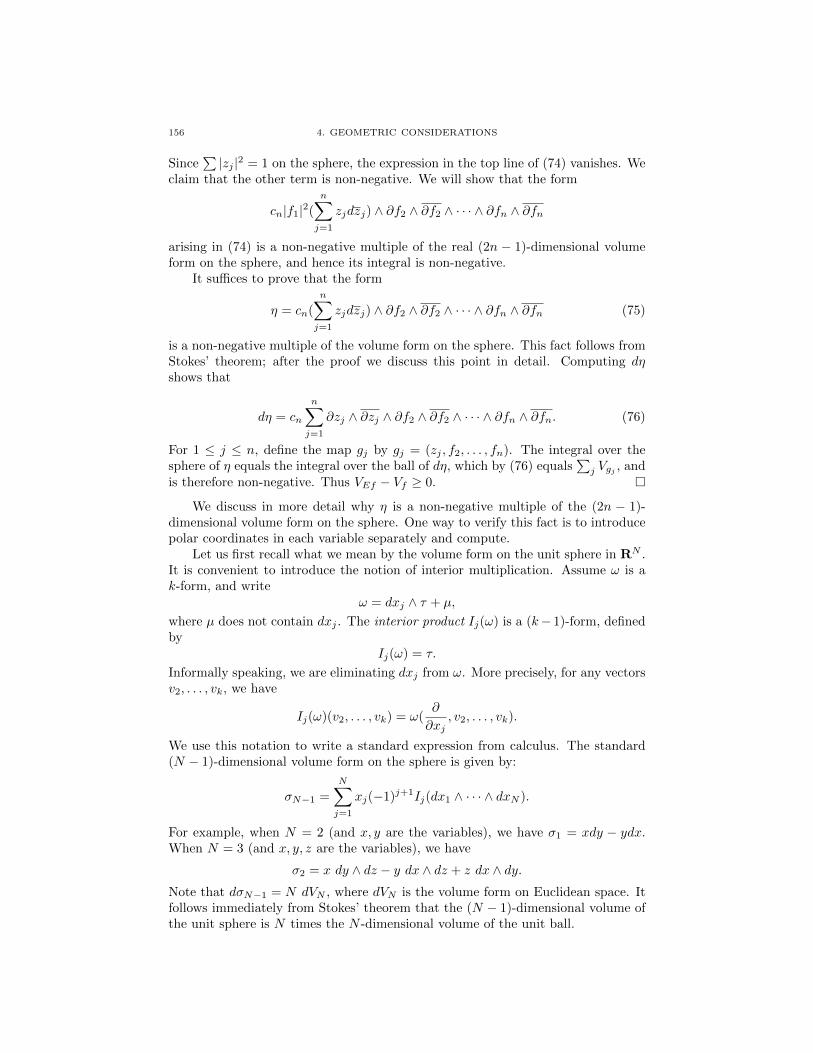
156 4. GEOMETRIC CONSIDERATIONS
Since∑|zj |2 = 1 on the sphere, the expression in the top line of (74) vanishes. We
claim that the other term is non-negative. We will show that the form
cn|f1|2(
n∑j=1
zjdzj) ∧ ∂f2 ∧ ∂f2 ∧ · · · ∧ ∂fn ∧ ∂fn
arising in (74) is a non-negative multiple of the real (2n − 1)-dimensional volumeform on the sphere, and hence its integral is non-negative.
It suffices to prove that the form
η = cn(
n∑j=1
zjdzj) ∧ ∂f2 ∧ ∂f2 ∧ · · · ∧ ∂fn ∧ ∂fn (75)
is a non-negative multiple of the volume form on the sphere. This fact follows fromStokes’ theorem; after the proof we discuss this point in detail. Computing dηshows that
dη = cn
n∑j=1
∂zj ∧ ∂zj ∧ ∂f2 ∧ ∂f2 ∧ · · · ∧ ∂fn ∧ ∂fn. (76)
For 1 ≤ j ≤ n, define the map gj by gj = (zj , f2, . . . , fn). The integral over thesphere of η equals the integral over the ball of dη, which by (76) equals
∑j Vgj , and
is therefore non-negative. Thus VEf − Vf ≥ 0.
We discuss in more detail why η is a non-negative multiple of the (2n − 1)-dimensional volume form on the sphere. One way to verify this fact is to introducepolar coordinates in each variable separately and compute.
Let us first recall what we mean by the volume form on the unit sphere in RN .It is convenient to introduce the notion of interior multiplication. Assume ω is ak-form, and write
ω = dxj ∧ τ + µ,
where µ does not contain dxj . The interior product Ij(ω) is a (k− 1)-form, definedby
Ij(ω) = τ.
Informally speaking, we are eliminating dxj from ω. More precisely, for any vectorsv2, . . . , vk, we have
Ij(ω)(v2, . . . , vk) = ω(∂
∂xj, v2, . . . , vk).
We use this notation to write a standard expression from calculus. The standard(N − 1)-dimensional volume form on the sphere is given by:
σN−1 =
N∑j=1
xj(−1)j+1Ij(dx1 ∧ · · · ∧ dxN ).
For example, when N = 2 (and x, y are the variables), we have σ1 = xdy − ydx.When N = 3 (and x, y, z are the variables), we have
σ2 = x dy ∧ dz − y dx ∧ dz + z dx ∧ dy.Note that dσN−1 = N dVN , where dVN is the volume form on Euclidean space. Itfollows immediately from Stokes’ theorem that the (N − 1)-dimensional volume ofthe unit sphere is N times the N -dimensional volume of the unit ball.

9. INEQUALITIES 157
Exercise 9.1. Verify the following formulas for the (N−1)-dimensional volumeWN of the unit sphere in RN :
• W1 = 2• W2 = 2π• W3 = 4π• W4 = 2π2
• W5 = 83π
2.
We are interested in the case where N = 2n is even, and we identify R2n withCn. In that case we can introduce polar coordinates in each variable separately.Thus zj = rje
iθj , where each rj is non-negative. On the unit sphere we have therelation
∑r2j = 1; it follows that
∑rjdrj = 0 on the sphere. We therefore use
all the θj as coordinates, but we use only r1, . . . , rn−1. The (2n − 1)-dimensionalvolume form on the sphere turns out to be (where the product is a wedge product)n−1∏
j=1
rjdrj ∧ dθj
∧ dθn.We continue this geometric approach by noting the following simple Lemma,
expressing the Cauchy-Riemann equations in polar coordinates.
Lemma 9.1. Assume h is complex analytic in one variable. Use polar coordi-nates z = reiθ. Then ∂h
∂θ = ri∂h∂r .
Proof. We will use subscripts to denote partial derivatives in this proof. Sinceh is complex analytic, hz = ∂h
∂z = 0. It follows that
hr =∂h
∂r=∂h
∂z
∂z
∂r= hze
iθ.
Similarly,
hθ =∂h
∂θ=∂h
∂z
∂z
∂θ= hzrie
iθ = rihr.
Remark 9.1. One can also prove Lemma 9.1 by observing that it suffices tocheck it for h(z) = zk.
Exercise 9.2. Prove Lemma 9.1 as suggested in the Remark.
A continuously differentiable function is complex analytic if and only if it iscomplex analytic in each variable separately. (The same conclusion holds withoutthe hypothesis of continuous differentiability, but this result, which we do not need,is much harder to prove.) The geometry of the sphere suggests, and the easierimplication justifies, working in polar coordinates in each variable separately.
Put zj = rjeiθj for 1 ≤ j ≤ n. Computation yields
dzj = eiθjdrj + irjeiθjdθj .
Note that∑n
1 rjdrj = 0 on the sphere. We compute∑n
1 zjdzj as follows:
n∑j=1
zjdzj =
n∑j=1
rjdrj − in∑j=1
r2jdθj = −i(
n∑j=1
r2jdθj).
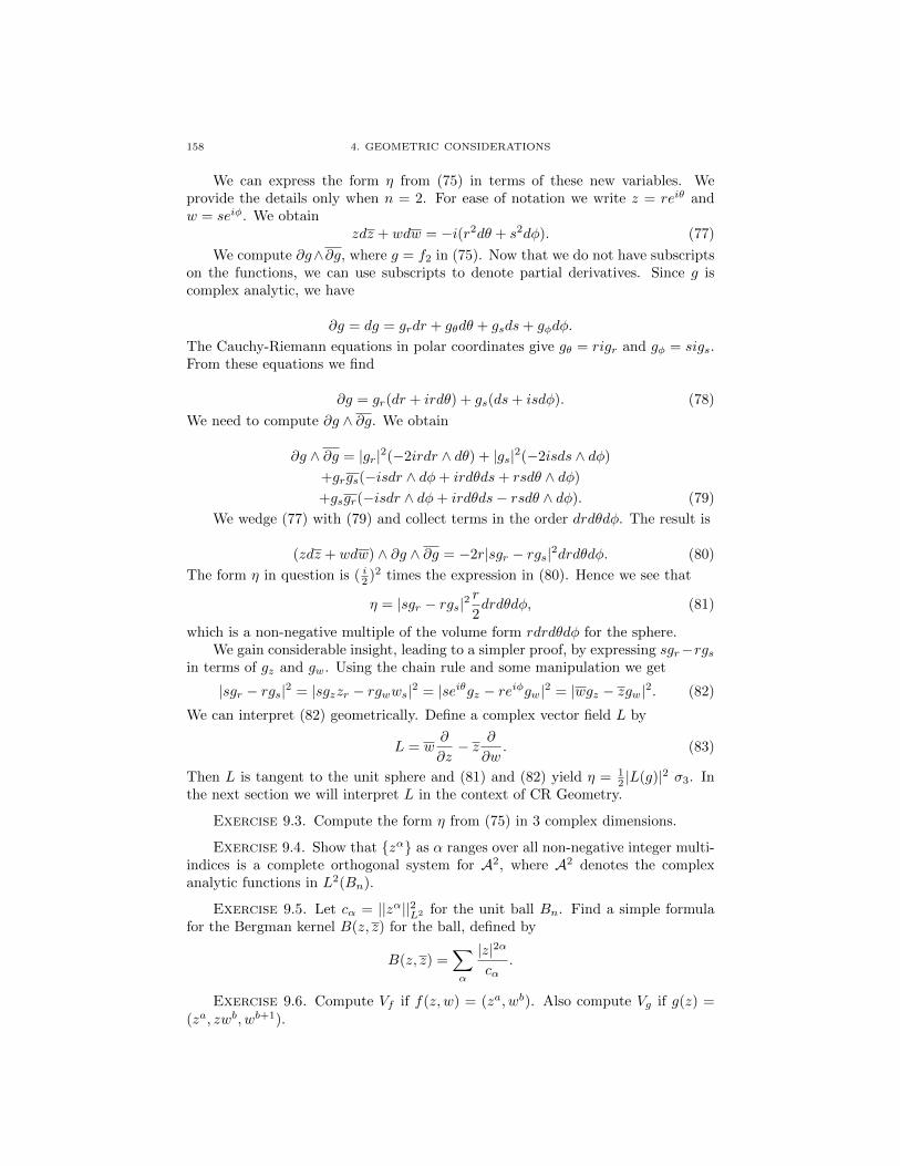
158 4. GEOMETRIC CONSIDERATIONS
We can express the form η from (75) in terms of these new variables. Weprovide the details only when n = 2. For ease of notation we write z = reiθ andw = seiφ. We obtain
zdz + wdw = −i(r2dθ + s2dφ). (77)
We compute ∂g∧∂g, where g = f2 in (75). Now that we do not have subscriptson the functions, we can use subscripts to denote partial derivatives. Since g iscomplex analytic, we have
∂g = dg = grdr + gθdθ + gsds+ gφdφ.
The Cauchy-Riemann equations in polar coordinates give gθ = rigr and gφ = sigs.From these equations we find
∂g = gr(dr + irdθ) + gs(ds+ isdφ). (78)
We need to compute ∂g ∧ ∂g. We obtain
∂g ∧ ∂g = |gr|2(−2irdr ∧ dθ) + |gs|2(−2isds ∧ dφ)
+grgs(−isdr ∧ dφ+ irdθds+ rsdθ ∧ dφ)
+gsgr(−isdr ∧ dφ+ irdθds− rsdθ ∧ dφ). (79)
We wedge (77) with (79) and collect terms in the order drdθdφ. The result is
(zdz + wdw) ∧ ∂g ∧ ∂g = −2r|sgr − rgs|2drdθdφ. (80)
The form η in question is ( i2 )2 times the expression in (80). Hence we see that
η = |sgr − rgs|2r
2drdθdφ, (81)
which is a non-negative multiple of the volume form rdrdθdφ for the sphere.We gain considerable insight, leading to a simpler proof, by expressing sgr−rgs
in terms of gz and gw. Using the chain rule and some manipulation we get
|sgr − rgs|2 = |sgzzr − rgwws|2 = |seiθgz − reiφgw|2 = |wgz − zgw|2. (82)
We can interpret (82) geometrically. Define a complex vector field L by
L = w∂
∂z− z ∂
∂w. (83)
Then L is tangent to the unit sphere and (81) and (82) yield η = 12 |L(g)|2 σ3. In
the next section we will interpret L in the context of CR Geometry.
Exercise 9.3. Compute the form η from (75) in 3 complex dimensions.
Exercise 9.4. Show that zα as α ranges over all non-negative integer multi-indices is a complete orthogonal system for A2, where A2 denotes the complexanalytic functions in L2(Bn).
Exercise 9.5. Let cα = ||zα||2L2 for the unit ball Bn. Find a simple formulafor the Bergman kernel B(z, z) for the ball, defined by
B(z, z) =∑α
|z|2α
cα.
Exercise 9.6. Compute Vf if f(z, w) = (za, wb). Also compute Vg if g(z) =(za, zwb, wb+1).
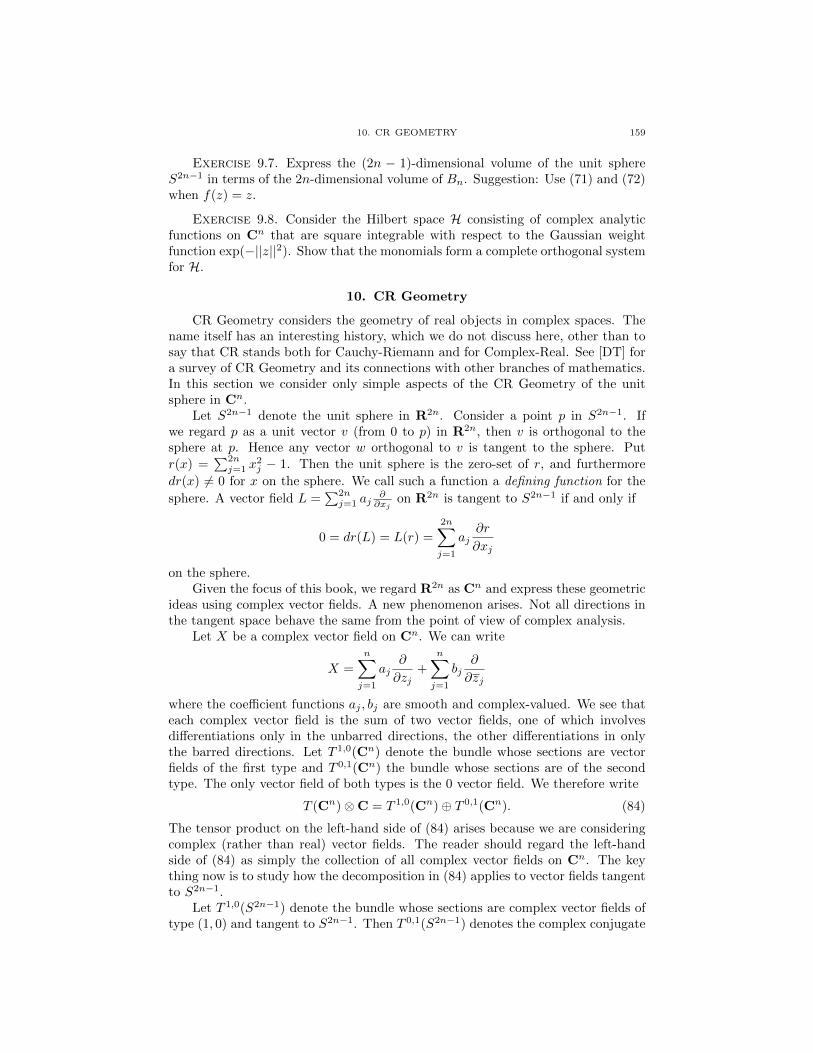
10. CR GEOMETRY 159
Exercise 9.7. Express the (2n − 1)-dimensional volume of the unit sphereS2n−1 in terms of the 2n-dimensional volume of Bn. Suggestion: Use (71) and (72)when f(z) = z.
Exercise 9.8. Consider the Hilbert space H consisting of complex analyticfunctions on Cn that are square integrable with respect to the Gaussian weightfunction exp(−||z||2). Show that the monomials form a complete orthogonal systemfor H.
10. CR Geometry
CR Geometry considers the geometry of real objects in complex spaces. Thename itself has an interesting history, which we do not discuss here, other than tosay that CR stands both for Cauchy-Riemann and for Complex-Real. See [DT] fora survey of CR Geometry and its connections with other branches of mathematics.In this section we consider only simple aspects of the CR Geometry of the unitsphere in Cn.
Let S2n−1 denote the unit sphere in R2n. Consider a point p in S2n−1. Ifwe regard p as a unit vector v (from 0 to p) in R2n, then v is orthogonal to thesphere at p. Hence any vector w orthogonal to v is tangent to the sphere. Putr(x) =
∑2nj=1 x
2j − 1. Then the unit sphere is the zero-set of r, and furthermore
dr(x) 6= 0 for x on the sphere. We call such a function a defining function for the
sphere. A vector field L =∑2nj=1 aj
∂∂xj
on R2n is tangent to S2n−1 if and only if
0 = dr(L) = L(r) =
2n∑j=1
aj∂r
∂xj
on the sphere.Given the focus of this book, we regard R2n as Cn and express these geometric
ideas using complex vector fields. A new phenomenon arises. Not all directions inthe tangent space behave the same from the point of view of complex analysis.
Let X be a complex vector field on Cn. We can write
X =
n∑j=1
aj∂
∂zj+
n∑j=1
bj∂
∂zj
where the coefficient functions aj , bj are smooth and complex-valued. We see thateach complex vector field is the sum of two vector fields, one of which involvesdifferentiations only in the unbarred directions, the other differentiations in onlythe barred directions. Let T 1,0(Cn) denote the bundle whose sections are vectorfields of the first type and T 0,1(Cn) the bundle whose sections are of the secondtype. The only vector field of both types is the 0 vector field. We therefore write
T (Cn)⊗C = T 1,0(Cn)⊕ T 0,1(Cn). (84)
The tensor product on the left-hand side of (84) arises because we are consideringcomplex (rather than real) vector fields. The reader should regard the left-handside of (84) as simply the collection of all complex vector fields on Cn. The keything now is to study how the decomposition in (84) applies to vector fields tangentto S2n−1.
Let T 1,0(S2n−1) denote the bundle whose sections are complex vector fields oftype (1, 0) and tangent to S2n−1. Then T 0,1(S2n−1) denotes the complex conjugate

160 4. GEOMETRIC CONSIDERATIONS
bundle. For p on the sphere, each of the vector spaces T 1,0p (S2n−1) and T 0,1
p (S2n−1)has complex dimension n− 1. Hence there is a missing direction. Observe that thecommutator [L,K] of vector fields L,K, each of type (1, 0) and tangent to S2n−1,also satisfies these properties. That [L,K] is of type (1, 0) follows easily from theformula [L,K] = LK−KL. That [L,K] is tangent follows by applying this formulato a defining function r: [L,K](r) = L(K(r)) − K(L(r)) = 0 − 0 = 0. Since Kis tangent, K(r) = 0 on the sphere. Since L is tangent, L(K(r)) = 0 there. Bysymmetry, K(L(r)) = 0 as well. Note the next remark.
Remark 10.1. Warning! Is the derivative of a constant zero? The functionR(x, y) = x2 +y2−1 equals 0 everywhere on the unit circle, but ∂R
∂x = 2x and henceis NOT zero at most points. The problem is that the differentiation with respectto x is not tangent to the unit circle.
We can abstract the geometry of the sphere as follows:
Definition 10.1. The CR structure on S2n−1 is given by the subbundle V =T 1,0(S2n−1) with the following properties:
(1) V ∩ V = 0.(2) The set of smooth sections of V is closed under the Lie bracket.(3) V ⊕ V has codimension one in T (S2n−1)⊗C.
More generally, a CR manifold of hypersurface type is a real manifold M forwhich there is a subbundle V ⊂ T (M) ⊗ C satisfying the three properties fromDefinition 10.1. For example, any real hypersurface in Cn is a CR manifold of hy-persurface type. See [DT] and its references for more information on CR structures.
Near a point where zn 6= 0, for 1 ≤ j ≤ n− 1, we define define n− 1 type (1, 0)vector fields by
Lj = zn∂
∂zj− zj
∂
∂zn. (85)
A simple check shows that each Lj is tangent to the sphere. Similarly the complex
conjugate vector fields Lj are tangent. These vector fields are linearly independent(as long as we are working where zn 6= 0). There are 2n − 2 of them. There isone missing direction, which requires both unbarred and barred derivatives. Forexample, we can fill out the complex tangent space by setting
T = zn∂
∂zn− zn
∂
∂zn. (86)
Then L1, . . . , Ln−1, L1, . . . , Ln−1, T span the complex tangent space to S2n−1 ateach point where zn 6= 0.
Exercise 10.1. Verify that the Lj from (85) and T from (86) are tangent tothe sphere.
Exercise 10.2. Compute the commutator (Definition 6.6) [Lj , Lk].
Exercise 10.3. Show that translating the sphere leads to the defining function
r(ζ, ζ) =
n−1∑j=1
|ζj |2 + |ζn|2 + 2Re(ζn). (87)
11. POSITIVITY CONDITIONS FOR HERMITIAN POLYNOMIALS 161
Show that a more elaborate change of variables leads to the defining function:
r(w,w) =
n−1∑j=1
|wj |2 + 2Re(wn) (88)
The zero-set of (88), a biholomorphic image of the sphere, is an unboundedobject H, commonly known as the Heisenberg group. Put n = 2 and define A by
A =∂
∂w1− w1
∂
∂w2.
Then A, A, and [A,A] form a basis for the sections of T (H)⊗C at each point. See[DT] and its references for considerable information about the role of the Heisenberggroup in complex analysis, geometry, and PDE.
We next use the CR geometry of the unit sphere to briefly study harmonicpolynomials. For simplicity we work on S3, where the vector field L from (83) de-fines the CR structure. Recall that (z, w) denotes the variable in C2. We also recallfrom Section 11 of Chapter 1 that a smooth function is harmonic if its Laplacianis 0. We can express the Laplace operator in terms of complex partial derivatives;a (possibly complex-valued) smooth function u is harmonic on C2 if and only if
uzz + uww = 0.
As in Section 13 from Chapter 2, it is natural to consider harmonic homoge-neous polynomials. Here we allow our harmonic functions to be complex-valued.The complex vector space Vd, consisting of homogeneous polynomials of degree d(with complex coefficients) in the underlying four real variables, decomposes into asum of spaces Vp,q. Here p+ q = d and elements of Vp,q are homogeneous of degreep in the (z, w) variables and of degree q in the conjugated variables. Similarly weobtain a further decomposition of the space of harmonic homogeneous polynomials.
Observe, for example, for each pair a, b of non-negative integers, that the mono-mials zawb and zawb are harmonic. By elementary calculus we see that
L(zawb) = aza−1wb+1
L(zawb) = −bza+1wb−1.
Combining these results shows that
LL(zawb) = −b(a+ 1)zawb.
LL(zawb) = −a(b+ 1)zawb
Thus the harmonic monomials zawb are eigenfunctions of the differential oper-ators LL and LL, with eigenvalues −b(a + 1) and −a(b + 1). Hence they are alsoeigenfunctions of the commutator T = [L,L], with eigenvalue a− b.
11. Positivity conditions for Hermitian polynomials
This section aims to glimpse recent research directions along the lines of thisbook. We state and discuss, but we do not prove, an analogue of the Riesz-Fejertheorem for positive polynomials on the unit sphere. We offer an application of thisresult to proper mappings between balls.
The Riesz-Fejer theorem (Theorem 3.1 of Chapter 1) characterizes non-negativetrig polynomials; each such polynomial agrees on the circle with the squared abso-lute value of a single polynomial in the complex variable z. We naturally seek to

162 4. GEOMETRIC CONSIDERATIONS
extend this result from the unit circle to the unit sphere in Cn. Things becomemore complicated but also more interesting.
We start with a Hermitian symmetric polynomial r(z, z) =∑α,β cαβz
αzβ ofdegree d in z ∈ Cn. We can always bihomogenize r by adding a variable as follows.We put (Hr)(0, 0) = 0. For z 6= 0 we put
(Hr)(z, t, z, t) = |t|2dr(zt,z
t).
Then Hr is homogeneous of degree d in the variables z, t and also homogeneous ofdegree d in their conjugates. The polynomial Hr is thus determined by its values onthe unit sphere in Cn+1. Conversely we can dehomogenize a bihomogeneous poly-nomial in two or more variables by setting one of its variables (and its conjugate!)equal to the number 1.
Example 11.1. Put r(z, z) = z2 + z2. We compute Hr:
(Hr)(z, t, z, t) = |t|4((z
t)2 + (
z
t)2) = t
2z2 + z2t2.
There is no loss in generality in our discussion if we restrict our attention tothe bihomogeneous case. Let R be a bihomogeneous polynomial in n variables (andtheir conjugates). Assume R(z, z) ≥ 0 on the unit sphere. As a generalization ofthe Riesz-Fejer theorem, we naturally ask if there exist homogeneous polynomialsf1(z), ..., fK(z) such that
R(z, z) = ||f(z)||2 =
K∑j=1
|fj(z)|2.
We call R a Hermitian sum of squares or Hermitian squared norm. Of course wecannot expectK to be any smaller than the dimension. For example, the polynomial∑nj=1 |zj |4 is positive on the sphere, but cannot be written as a Hermitian squared
norm with fewer terms. Furthermore, not every non-negative R is a Hermitiansquared norm. Even restricted to the unit sphere, such a result fails in general, andhence the analogue of the Riesz-Fejer theorem is more subtle.
Example 11.2. Put R(z, z) = (|z1|2 − |z2|2)2. Then R is bihomogeneous andnon-negative. Its underlying matrix Cαβ of coefficients is diagonal with eigenvalues1,−2, 1. Suppose for some f that R(z, z) = ||f(z)||2. Then f would vanish on thesubset of the unit sphere defined by |z1|2 = |z2|2 = 1
2 (a torus), because R does.
A complex analytic function vanishing there would also vanish for |z1|2 ≤ 12 and
|z2|2 ≤ 12 by the maximum principle. Hence f would have to be identically zero.
Thus R does not agree with a squared norm of any complex analytic mapping. Thezero-set of R does not satisfy appropriate necessary conditions here.
The following elaboration of Example 11.2 clarifies the matter. Consider thefamily of polynomials Rε defined by
Rε(z, z) = (|z1|2 − |z2|2)2 + ε|z1|2|z2|2.
For each ε > 0, we have Rε(z, z) > 0 on the sphere. By Theorem 11.2 below thereis a polynomial mapping fε such that Rε = ||fε||2 on the sphere. Both the degreeand the number of components of fε must tend to infinity as ε tends to 0. See [D1]for a lengthy discussion of this sort of issue.
11. POSITIVITY CONDITIONS FOR HERMITIAN POLYNOMIALS 163
From Example 11.2 we discover that non-negativity is too weak of a conditionto imply that R agrees with a Hermitian squared norm. See also Example 11.4.On the other hand, when R(z, z) > 0 on the sphere, the conclusion does hold. See[D1] for detailed proofs of Theorem 11.1 and Theorem 11.2 below. The proof ofTheorem 11.1 there uses the theory of compact operators, but other proofs havebeen found.
Theorem 11.1. Let r be a Hermitian symmetric bihomogeneous polynomial inn variables and their conjugates. Suppose r(z, z) > 0 on the unit sphere. Thenthere are positive integers d and K, and a polynomial mapping g : Cn → CK , suchthat
||z||2dr(z, z) = ||g(z)||2.
We can remove the assumption of bihomogeneity if we want equality to holdonly on the unit sphere.
Theorem 11.2. Let r be a Hermitian symmetric polynomial in n variables andtheir conjugates. Assume that r(z, z) > 0 on the unit sphere. Then there are aninteger N and a polynomial mapping h such that, for z on the unit sphere,
r(z, z) = ||h(z)||2.
Proof. We sketch the derivation of Theorem 11.2 from Theorem 11.1. Firstwe bihomogenize r to get (Hr)(z, t, z, t), bihomogeneous of degree m in the z, tvariables. We may assume m is even. The polynomial Hr could have negativevalues on the sphere ||z||2 + |t|2 = 1. To correct for this possibility, we define abihomogeneous polynomial FC by
FC(z, z, t, t) = (Hr)(z, t, z, t) + C(||z||2 − |t|2)m.
It is easy to show that we can choose C large enough to make FC strictly positiveaway from the origin. By Theorem 11.1, we can find an integer d such that
(||z||2 + |t|2)dFC(z, z, t, t) = ||g(z, t)||2.
Setting t = 1 and then ||z||2 = 1 shows that
2dr(z, z) = ||g(z, 1)||2
on the unit sphere.
The following Corollary of Theorem 11.2 connects these ideas with proper com-plex analytic mappings between balls.
Corollary 11.1. Let f = pq : Ω ⊂ Cn → CN be a rational mapping. (Here
Ω is the complement of the zero set of the denominator q.) Assume that the imageof the closed unit ball under f lies in the open unit ball in CN . Then there are aninteger K and a polynomial mapping g : Cn → CK such that p⊕g
q maps the unit
sphere S2n−1 to the unit sphere S2(N+K)−1.
Proof. The hypothesis implies that |q|2 − ||p||2 is strictly positive on thesphere. By Theorem 11.2 there is a polynomial map g such that |q|2−||p||2 = ||g||2on the sphere. Then p⊕g
q does the job.

164 4. GEOMETRIC CONSIDERATIONS
This corollary implies that there are many rational mappings taking the unitsphere in the domain into the unit sphere in some target. We choose the first severalcomponents to be anything we want, as long as the closed ball gets mapped to theopen ball. Then we can find additional components, using the same denominator,such that the resulting map takes the sphere to the sphere. The following simpleexample already indicates the depth of these ideas.
Example 11.3. Consider the maps pλ : C2 → C given by pλ(z, w) = λzw.Then pλ maps the closed ball in C2 inside the unit disk if |λ|2 < 4. If this conditionis met, then we can include additional components to make pλ into a componentof a polynomial mapping sending S3 to some unit sphere. In case λ =
√3, we
obtain the map (√
3zw, z3, w3), which is one of the group-invariant examples from
Section 3. If√
3 < λ < 2, then we must map into a dimension higher than 3. As λapproaches 2, the minimum possible target dimension approaches infinity.
We close this chapter with a surprising example from [D1] that combines ideasfrom several parts of this book.
Example 11.4. There exists a bihomogeneous polynomial r(z, z), in three vari-ables, with the following properties:
• r(z, z) ≥ 0 for all z.• The zero set of r is a copy of C.• 0 is the only polynomial s for which rs is a Hermitian squared norm.
We put r(z, z) = (|z1z2|2 − |z3|4)2 + |z1|8. The non-negativity is evident. Thezero-set of r is the set of z of the form (0, z2, 0), and hence a copy of C. Assumethat rs is a Hermitian squared norm ||A||2. Consider the map from C to C3 givenby t 7→ (t2, 1 + t, t) = z(t). Pulling back yields the equation
r(z(t), z(t)) s(z(t), z(t)) = ||cmtm + · · · ||2,where · · · denotes higher order terms. Hence the product of the lowest order termsin the pullback of s with the lowest order terms in the pullback of r is ||cm||2|t|2m.A simple computation shows that the lowest order terms in the pullback of r are
t4t6
+ 2|t|10 + t6t4
= 2|t|10(1 + cos(2θ)). (89)
One cannot multiply the right-hand side of (89) by an expression of the form|t|2kp(θ) and obtain a result independent of θ, unless that expression is 0.
No such example is possible in one dimension, because the only bihomogeneouspolynomials are of the form c|t|2m. It is easy to find a non-negative polynomialg(t, t) that doesn’t divide any Hermitian squared norm (other than 0); for example,
2|t|2 + t2 + t2
= 2|t|2(1 + cos(2θ))
does the job. Our example is surprising because r is bihomogeneous.

CHAPTER 5
Appendix
1. The real and complex number systems
In this appendix we organize some of the mathematical prerequisites for readingthis book. The reader must be thoroughly informed about basic real analysis andshould know a bit of complex variable theory.
The real number system R is characterized by being a complete ordered field.The field axioms enable the usual operations of addition, subtraction, multiplica-tion, and division (except by 0). These operations satisfy familiar laws. The orderaxioms allow us to manipulate inequalities as usual. The completeness axiom ismore subtle; this crucial property distinguishes R from the rational number systemQ. One standard way to state the completeness axiom uses the least upper boundproperty:
Definition 1.1. If S is a non-empty subset of R and S is bounded above, thenS has a least upper bound α, written sup(S), and called the supremum of S.
Recall that a sequence of real numbers is a function n → xn from the naturalnumbers to R. (Sometimes we also allow the indexing to begin with 0.) Thesequence xn converges to the real number L if, for all ε > 0, there is an integerNε such that n ≥ Nε implies |xn − L| < ε.
The least upper bound property enables us to prove that a bounded monotonenondecreasing sequence xn of real numbers converges to the supremum of thevalues of the sequence. It also enables a proof of the fundamental result of basicreal analysis: a sequence of real numbers converges if and only if it is a Cauchysequence. Recall that a sequence is Cauchy if, for every ε > 0, there is an Nε suchthat n,m ≥ Nε implies |xn − xm| < ε. Thus a sequence has a limit L if the termsare eventually as close to L as we wish, and a sequence is Cauchy if the terms areeventually all as close to each other as we wish. The equivalence of the conceptssuggests that the real number system has no gaps.
For clarity we highlight these fundamental results as a theorem. The ability toprove Theorem 1.1 should be regarded as a prerequisite for reading this book.
Theorem 1.1. If a sequence xn of real numbers is bounded and monotone,then xn converges. A sequence xn converges to a real number L if and only ifxn is Cauchy.
Corollary 1.1. A monotone sequence converges if and only if it is bounded.
Remark 1.1. The first statement in Theorem 1.1 is considerably easier thanthe second. It is possible to prove the difficult (if) part of the second statementby extracting a monotone subsequence and using the first part. It is also possibleto prove the second statement by using the Bolzano-Weierstrass property fromTheorem 2.6 below.
165

166 5. APPENDIX
The complex number system C is a field, but it has no ordering. As a set C issimply the Euclidean plane R2. We make this set into a field by defining additionand multiplication:
(x, y) + (a, b) = (x+ a, y + b)
(x, y) ∗ (a, b) = (xa− yb, xb+ ya).
The additive identity 0 is then the ordered pair (0, 0) and the multiplicative identity1 is the pair (1, 0). Note that (0, 1) ∗ (0, 1) = (−1, 0) = −(1, 0). As usual we denote(0, 1) by i and then write x + iy instead of (x, y). We then drop the ∗ from thenotation for multiplication, and the law becomes obvious. Namely, we expand(x+ iy)(a+ ib) by the distributive law and set i2 = −1. These operations make R2
into a field called C.Given z = x+ iy we write z = x− iy and call z the complex conjugate of z. We
define |z| to be the Euclidean distance of z to 0; thus |z| =√x2 + y2 and |z|2 = zz.
The non-negative real number |z − w| equals the Euclidean distance betweencomplex numbers z and w. The following properties of distance make C into acomplete metric space. (See the next section.)
• |z − w| = 0 if and only if z = w.• |z − w| ≥ 0 for all z and w.• |z − w| = |w − z| for all z and w.• |z − w| ≤ |z − ζ|+ |ζ − w| for all z, w, ζ. (the triangle inequality)
Once we know that |z − w| defines a distance, we can repeat the definition ofconvergence.
Definition 1.2. Let zn be a sequence of complex numbers, and supposeL ∈ C. We say that zn converges to L if, for all ε > 0, there is an Nε such thatn ≥ Nε implies |zn − L| < ε.
Let an be a sequence of complex numbers. We say that∑∞n=1 an converges
to L, if
limN→∞
N∑n=1
an = L.
We say that∑∞n=1 an converges absolutely if
∑∞n=1 |an| converges. It is often easy
to establish absolute convergence; a series of non-negative numbers converges ifand only if the sequence of partial sums is bounded. The reason is simple: if theterms of a series are non-negative, then the partial sums form a monotone sequence,and hence the sequence of partial sums converges if and only if it is bounded. SeeCorollary 1.1 above. We also use the following standard comparison test; we includethe proof because it beautifully illustrates the Cauchy convergence criterion.
Proposition 1.1. Let zn be a sequence of complex numbers. Assume for alln that |zn| ≤ cn, and that
∑∞n=1 cn converges. Then
∑∞n=1 zn converges.
Proof. Let SN denote the N -th partial sum of the series∑zn, and let TN
denote the N -th partial sum of the series∑cn. For M > N we have
|SM − SN | = |M∑N+1
zn| ≤M∑N+1
|zn| ≤M∑N+1
cn = TM − TN . (1)

1. THE REAL AND COMPLEX NUMBER SYSTEMS 167
Since∑cn is convergent, TN is a Cauchy sequence of real numbers. By (1),
SN is also Cauchy, and hence∑∞n=1 zn converges by Theorem 1.1.
We pause to recall and discuss the notion of equivalence class, which we presumeis familiar to the reader. Let S be a set. An equivalence relation on S is a relation∼ such that, for all a, b, c ∈ S,
Reflexive property: a ∼ aSymmetric property: a ∼ b if and only if b ∼ aTransitive property: a ∼ b and b ∼ c implies a ∼ c.
Given an equivalence relation on a set S, we can form a new set, sometimeswritten S/ ∼, as follows. We say that a and b are equivalent, or lie in the sameequivalence class, if a ∼ b holds. The elements of S/ ∼ are the equivalence classes;the set S/ ∼ is called the quotient space.
We mention three examples. The first is trivial, the second is easy but funda-mental, and the third is profound.
Example 1.1. Let S be the set of ordered pairs (a, b) of integers. We say that(a, b) ∼ (c, d) if 100a + b = 100c + d. If we regard the first element of the orderedpair as the number of dollars, and the second element as the number of cents, thentwo pairs are equivalent if they represent the same amount of money. (Note thatwe allow negative money here.)
Example 1.2. Let S be the set of ordered pairs (a, b) of integers, with b 6= 0.We say that (a, b) ∼ (A,B) if aB = Ab. The equivalence relation restates, withoutmentioning division, the condition that a
b and AB define the same rational number.
Then S/ ∼ is the set of rational numbers. It becomes the system Q after we defineaddition and multiplication of equivalence classes and verify the required properties.
Example 1.3. The real number system R is sometimes defined to be the com-pletion of the rational number system Q. In this definition, a real number is anequivalence class of Cauchy sequences of rational numbers. Here we define a se-quence of rational numbers qn to be Cauchy if, for each positive integer K, wecan find a positive integer N such that m,n ≥ N implies |qm − qn| < 1
K . (The
number 1K plays the role of ε; we cannot use ε because real numbers have not yet
been defined!) Two Cauchy sequences are equivalent if their difference convergesto 0. Thus Cauchy sequences pn and qn of rational numbers are equivalent if,for every M ∈ N, there is an N ∈ N such that |pn − qn| < 1
M whenever n ≥ N .Intuitively, we can regard a real number to be the collection of all sequences ofrational numbers which appear to have the same limit. We use the language of thenext section; as a set, R is the metric space completion of Q. As in Example 1.2,we need to define addition, multiplication, and order and establish their propertiesbefore we get the real number system R.
We are also interested in convergence issues in higher dimensions. Let Rn
denote real Euclidean space of dimension n and Cn denote complex Euclideanspace of dimension n. In the next paragraph, we let F denote either R or C.
As a set, Fn consists of all n-tuples of elements of the field F. We writez = (z1, . . . , zn) for a point in Fn. This set has the structure of a real or complexvector space with the usual operations of vector addition and scalar multiplication:
(z1, z2, . . . , zn) + (w1, w2, . . . , wn) = (z1 + w1, z2 + w2, . . . , zn + wn).

168 5. APPENDIX
c(z1, z2, . . . , zn) = (cz1, cz2, . . . , czn)
Definition 1.3 (norm). A norm on a real or complex vector space V is afunction v 7→ ||v|| satisfying the following three properties:
(1) ||v|| > 0 for all nonzero v.(2) ||cv|| = |c| ||v|| for all c ∈ C and all v ∈ V .(3) (The triangle inequality) ||v + w|| ≤ ||v||+ ||w|| for all v, w ∈ V .
We naturally say normed vector space for a vector space equipped with a norm.We can make a normed vector space into a metric space by defining d(u, v) =||u− v||.
For us the notations Rn and Cn include the vector space structure and theEuclidean squared norm defined by (2):
||z||2 = 〈z, z〉. (2)
These norms come from the Euclidean inner product. In the real case we have
〈x, y〉 =
n∑j=1
xjyj (3.1)
and in the complex case we have
〈z, w〉 =
n∑j=1
zjwj . (3.2)
In both cases ||z||2 = 〈z, z〉.
2. Metric spaces
The definitions of convergent sequence in various settings are so similar that itis natural to put these settings into one abstract framework. One such setting ismetric spaces.
We assume that the reader is somewhat familiar with metric spaces. We recallthe definition and some basic facts. Let R+ denote the non-negative real numbers.
Definition 2.1. Let X be a set. A distance function on X is a functiond : X ×X → R+ satisfying the following properties:
(1) d(x, y) = 0 if and only if x = y.(2) d(x, y) = d(y, x) for all x, y.(3) d(x, z) ≤ d(x, y) + d(y, z) for all x, y, z.
If d is a distance function on X, then the pair (X, d) is called a metric space and dis called the metric.
The real numbers, the complex numbers, real Euclidean space, and complexEuclidean space are all metric spaces under the usual Euclidean distance function.One can define other metrics, with very different properties, on these sets. Forexample, on any set X, the function d : X × X → R+, defined by d(x, y) = 1 ifx 6= y and d(x, x) = 0, is a metric. In general sets admit many different usefuldistance functions. When the metric is understood, one often says “Let X be ametric space”. This statement is convenient but a bit imprecise.
Metric spaces provide a nice conceptual framework for convergence.
2. METRIC SPACES 169
Definition 2.2. Let xn be a sequence in a metric space (X, d). We saythat xn converges to x if, for all ε > 0, there is an N such that n ≥ N impliesd(xn, x) < ε. We say that xn is Cauchy if, for all ε > 0, there is an N such thatm,n ≥ N implies d(xm, xn) < ε.
Definition 2.3. A metric space (M,d) is complete if every Cauchy sequenceconverges.
If a metric space (M,d) is not complete, then we can form a new metric spacecalled its completion. The idea precisely parallels the construction of R given Q.The completion consists of equivalence classes of Cauchy sequences of elements of(M,d). The distance function extends to the larger set by taking limits.
Here are several additional examples of metric spaces. We omit the neededverifications of the properties of the distance function, but we mention that insome instances proving the triangle inequality requires effort.
Example 2.1. Let X be the space of continuous functions on [0, 1]. Define
d(f, g) =∫ 1
0|f(x) − g(x)|dx. Then (X, d) is a metric space. More generally, for
1 ≤ p <∞, we define dp(f, g) by
dp(f, g) =
(∫ 1
0
|f(x)− g(x)|pdx) 1p
.
We define d∞(f, g) by d∞(f, g) = sup|f − g|.
Of these examples, only (X, d∞) is complete. Completeness in this case followsbecause the uniform limit of a sequence of continuous functions is itself continuous.
A subset Ω of a metric space is called open if, whenever p ∈ Ω, there is a positiveε such that x ∈ Ω whenever d(p, x) < ε. In particular the empty set is open andthe whole space X is open. A subset K is called closed if its complement is open.
Proposition 2.1. Let (X, d) be a metric space. Let K ⊂ X. Then K is closedif and only if, whenever xn is a sequence in K, and xn converges to x, thenx ∈ K.
Proof. Left to the reader.
Let (M,d) and (M ′, d′) be metric spaces. The natural collection of maps be-tween them is the set of continuous functions.
Definition 2.4 (Continuity). f : (M,d)→ (M ′, d′) is continuous if, wheneverU is open in M ′, then f−1(U) is open in M .
Proposition 2.2. Suppose f : (M,d) → (M ′, d′) is a map between metricspaces. The following are equivalent:
(1) f is continuous(2) Whenever xn converges to x in M , then f(xn) converges to f(x) in M ′.(3) For all ε > 0, there is a δ > 0 such that
d(x, y) < δ =⇒ d′(f(x), f(y)) < ε.
Exercise 2.1. Prove Propositions 2.1 and 2.2.
We next mention several standard and intuitive geometric terms. The interiorof a set S in a metric space is the union of all open sets contained in S. The closure

170 5. APPENDIX
of a set S is the intersection of all closed sets containing S. Thus a set is open if andonly if it equals its interior, and a set is closed if and only if it equals its closure.The boundary bΩ of a set Ω consists of all points in the closure of Ω but not in theinterior of Ω. Another way to define boundary is to note that x ∈ bΩ if and onlyif, for every ε > 0, the ball of radius ε about x has a non-empty intersection withboth Ω and its complement.
Continuity often gets used together with the notion of a dense subset of a metricspace M . A subset S is dense if each x ∈M is the limit of a sequence of points inS. In other words, M is the closure of S. For example, the rational numbers aredense in the real numbers. If f is continuous on M , then f(x) = limn f(xn), andhence f is determined by its values on a dense set.
One of the most important examples of a metric space is the collection C(M)of continuous complex-valued functions on a metric space M . Several times inthe book we use compactness properties in C(M). We define compactness in thestandard open cover fashion, called the Heine-Borel property. What matters mostfor us is the Bolzano-Weierstrass property.
We quickly review some of the most beautiful results in basic analysis.
Definition 2.5. Let M be a metric space and let K ⊂ M . K is compactif, whenever K is contained in an arbitrary union ∪Aα of open sets, then K iscontained in a finite union ∪Nk=1Ajk of these open sets. This condition is called theHeine-Borel property.
This definition of compact is often stated informally “every open cover has afinite subcover”, but these words are a bit imprecise.
Definition 2.6. Let (M,d) be a metric space. A subset K ⊂ M satisfies theBolzano-Weierstrass property if, whenever xn is a sequence in K, then there is asubsequence xnk converging to a limit in K.
Theorem 2.1. Let (M,d) be a metric space and let K ⊂ M . Then K iscompact if and only if K satisfies the Bolzano-Weierstrass property.
Theorem 2.2. A subset of Euclidean space is compact if and only if it is closedand bounded.
Exercise 2.2. Prove Theorems 2.1 and 2.2.
Definition 2.7 (Equicontinuity). A collection K of complex-valued functionson a metric space (M,d) is called equicontinuous if, for all x and for all ε > 0, thereis a δ > 0 such that
d(x, y) < δ =⇒ |f(x)− f(y)| < ε
for all f ∈ K.
Definition 2.8 (Uniformly bounded). A collection K of complex-valued func-tions on a metric space (M,d) is called uniformly bounded if there is a C such that|f(x)| ≤ C for all x ∈M and for all f ∈ K.
We refer to [F1] for a proof of the following major result in analysis. Thestatement and proof in [F1] apply in the more general context of locally compactHausdorff topological spaces. In this book we use Theorem 2.3 to show that certainintegral operators are compact. See Sections 10 and 11 of Chapter 2.

3. INTEGRALS 171
Theorem 2.3 (Arzela-Ascoli theorem). Let M be a compact metric space. LetC(M) denote the continuous functions on M with d(f, g) = supM |f(x)−g(x)|. LetK be a subset of C(M). Then K is compact if and only if the following three itemsare true:
(1) K is equicontinuous.(2) K is uniformly bounded.(3) K is closed.
Corollary 2.1. Let K be a closed, uniformly bounded, and equicontinuoussubset of C(M). Let fn be a sequence in K. Then fn has a convergent subse-quence. That is, fnk converges uniformly to an element of K.
Proof. By the theoremK is compact; the result then follows from the Bolzano-Weierstrass characterization of compactness.
Exercise 2.3. Let M be a compact subset of Euclidean space. Fix α > 0. LetHα denote the subset of C(M) satisfying the following properties:
(1) ||f ||∞ ≤ 1.(2) ||f ||Hα ≤ 1. Here
||f ||Hα = supx6=y
|f(x)− f(y)||x− y|α
.
Show that Hα is compact.
A function f for which ||f ||Hα is finite is said to satisfy a Holder condition oforder α. See Definition 9.1 of Chapter 2.
3. Integrals
This book presumes that the reader knows the basic theory of the Riemann-Darboux integral, which we summarize. See [Ro] among many possible texts.
Let [a, b] be a closed bounded interval on R, and suppose f : [a, b] → R is a
bounded function. We define∫ baf(t)dt by a standard but somewhat complicated
procedure. A partition P of [a, b] is a finite collection of points pj such that a =p0 < · · · < pj < · · · < pN = b. Given f and a partition P , we define the lower andupper sums corresponding to the partition:
L(f, P ) =
N∑j=1
(pj − pj−1)inf [pj−1,pj ](f(x))
U(f, P ) =
N∑j=1
(pj − pj−1)sup[pj−1,pj ](f(x)).
Definition 3.1. A bounded function f : [a, b] → R is Riemann integrable if
supPL(f, P ) = infPU(f, P ). If so, we denote the common value by∫ baf(t)dt or
simply by∫ baf .
An equivalent way to state Definition 3.1 is that f is integrable if, for eachε > 0, there is a partition Pε such that U(f, Pε)− L(f, Pε) < ε.

172 5. APPENDIX
In case f is complex-valued, we define it to be integrable if its real and imaginaryparts are integrable, and we put∫ b
a
f =
∫ b
a
u+ iv =
∫ b
a
u+ i
∫ b
a
v.
The integral satisfies the usual properties:
(1) If f, g are Riemann integrable on [a, b], and c is a constant, then f +g andcf are Riemann integrable and∫ b
a
f + g =
∫ b
a
f +
∫ b
a
g,
∫ b
a
cf = c
∫ b
a
f.
(2) If f is Riemann integrable and f(x) ≥ 0 for x ∈ [a, b], then∫ baf ≥ 0.
(3) If f is continuous on [a, b], then f is Riemann integrable.(4) If f is monotone on [a, b], then f is Riemann integrable.
We assume various other basic results, such as the change of variables formula,without further mention.
The collection of complex-valued integrable functions on [a, b] is a complex vec-tor space. We would like to define the distance δ(f, g) between integrable functionsf and g by
δ(f, g) = ||f − g||L1 =
∫ b
a
|f(x)− g(x)|dx,
but a slight problem arises. If f and g agree for example everywhere except at asingle point, and each is integrable, then δ(f, g) = 0 but f and g are not the samefunction. This point is resolved by working with equivalence classes of functions.Two functions are called equivalent if they agree except on what is called a set ofmeasure zero. See Section 7 of Chapter 1. Even after working with equivalenceclasses, this vector space is not complete (in the metric space sense). One needs touse the Lebesgue integral to identify its completion.
Often one requires so-called improper integrals. Two possible situations arise;one is when f is unbounded on [a, b], the other is when the interval is unbounded.Both situations can happen in the same example. The definitions are clear, and westate them informally. If f is unbounded at a, for example, but Riemann integrableon [a+ ε, b] for all positive ε, then we define∫ b
a
f = limε→0
∫ b
a+ε
f
if the limit exists. If f is Riemann integrable on [a, b] for all b, then we put∫ ∞a
f = limb→∞
∫ b
a
f.
The other possibilities are handled in a similar fashion. Here are two simple exam-ples of improper integrals:
(1)∫ 1
0xαdx = 1
α+1 if α > −1.
(2)∫∞
0e−xdx = 1.

4. EXPONENTIALS AND TRIG FUNCTIONS 173
At several points in this book, whether an improper integral converges will besignificant. We mention specifically Section 8 of Chapter 3, where one shows thata function has k continuous derivatives by showing that an improper integral isconvergent.
The following theorem is fundamental to all that we do in this book.
Theorem 3.1 (Fundamental theorem of calculus). Assume f is continuous on[a, b]. For x ∈ (a, b) put F (x) =
∫ xaf(t)dt. Then F is differentiable and F ′(x) =
f(x).
Exercise 3.1. Establish the above properties of the Riemann integral.
Exercise 3.2. Verify that∫ bacf = c
∫ baf when c is complex and f is complex-
valued. Check that Re(∫ baf) =
∫ ba
Re(f) and similarly with the imaginary part.
Exercise 3.3. Verify the improper integrals above.
Exercise 3.4. For p a positive integer, prove that∫ 1
0tpdt = 1
p+1 by using the
definition of the Riemann integral. (Find upper and lower sums.)
Exercise 3.5. Prove the fundamental theorem of calculus. The idea of itsproof recurs throughout this book.
4. Exponentials and trig functions
The unit circle is the set of complex numbers of unit Euclidean distance from0, that is, the set of z with |z| = 1.
The complex exponential function is defined by
ez =
∞∑n=0
zn
n!.
The series converges absolutely for all complex z. Furthermore the resultingfunction satisfies e0 = 1 and ez+w = ezew for all z and w.
We define the complex trig functions by
cos(z) =eiz + e−iz
2
sin(z) =eiz − e−iz
2i.
When z is real these functions agree with the usual trig functions. The reader whoneeds convincing can express both sides as power series.
Note, by continuity of complex conjugation, we have ez = ez. Combining thisproperty with the addition law gives (assuming t is real)
1 = e0 = eite−it = |eit|2.
Thus z = eit lies on the unit circle. Its real part x is given by x = z+z2 and its
imaginary part y is given by y = z−z2i . Comparing with our definitions of cosine and
sine, we obtain the famous Euler identity (which holds even when t is complex):
eit = cos(t) + isin(t).

174 5. APPENDIX
Complex logarithms are quite subtle. For a positive real number t we definelog(t), sometimes written ln(t), by the usual formula
log(t) =
∫ t
1
du
u.
For a nonzero complex number z, written in the form z = |z|eiθ, we provisionallydefine its logarithm by
log(z) = log(|z|) + iθ. (4)
The problem with this formula is that θ is defined only up to multiples of 2π. Wemust therefore restrict θ to an interval of length 2π. In order that the logarithmbe continuous, we must choose a branch cut. Thus we first choose an open intervalof length 2π, and then we define the logarithm only for θ in that open interval.Doing so yields a branch of the logarithm. For example, we often write (4) for0 6= z = |z|eiθ and −π < θ < π. Combining the identity eα+β = eαeβ with (4), weobtain elog(z) = |z|eiθ = z.
5. Complex analytic functions
The geometric series arises throughout mathematics. Suppose that z is a com-plex number not equal to 1. Then we have the finite geometric series
n−1∑j=0
zj =1− zn
1− z.
When |z| < 1, we let n→∞ and obtain the geometric series
∞∑j=0
zj =1
1− z.
The geometric series and the exponential series lie at the foundation of complexanalysis. We have seen how the exponential function informs trigonometry. Thegeometric series enables the proof of Theorem 4.1 below; the famous Cauchy integralformula combines with the geometric series to show that an arbitrary complexanalytic function has a local power series expansion.
A subset Ω of C is called open if, for all p ∈ Ω, there is an open ball about pcontained in Ω. In other words, there is a positive ε such that |z − p| < ε impliesz ∈ Ω. Suppose that Ω is open and f : Ω → C is a function. We say that f iscomplex analytic on Ω if, for each z ∈ Ω, f is complex differentiable at z. (in otherwords, if the limit in (5) exists).
limh→0
f(z + h)− f(z)
h= f ′(z) (5)
A continuously differentiable function f : Ω→ C satisfies the Cauchy-Riemannequations if ∂f∂z = 0 at all points of Ω. The complex partial derivative is defined by
∂
∂z=
1
2(∂
∂x+ i
∂
∂y).
In most elementary books on complex variables, one writes f = u+ iv in terms ofits real and imaginary parts, and writes the Cauchy-Riemann equations as the pair
6. PROBABILITY 175
of equations∂u
∂x=∂v
∂y
∂u
∂y= −∂v
∂x.
Perhaps the most fundamental theorem in basic complex analysis relates com-plex analytic functions, convergent power series, and the Cauchy-Riemann equa-tions. Here is the precise statement:
Theorem 5.1. Assume that Ω is open and f : Ω → C is a function. Thefollowing are equivalent:
(1) f is complex analytic on Ω.(2) For all p in Ω, there is a ball about p on which f is given by a convergent
power series:
f(z) =
∞∑n=0
an(z − p)n.
(3) f is continuously differentiable and ∂f∂z = 0 on Ω.
We close this review of complex variable theory by recalling the FundamentalTheorem of Algebra. Many proofs are known, but all of them require the methodsof analysis. No purely algebraic proof can exist.
Theorem 5.2 (Fundamental theorem of algebra). Let p(z) be a non-constantpolynomial with complex coefficients and of degree d. Then p factors into a productof d linear factors:
p(z) = c
d∏j=1
(z − zj),
where the zj may be repeated.
6. Probability
Many of the ideas in this book are closely connected with probability theory.We barely glimpse these connections.
We begin by briefly mentioning probability densities. See a good text such as[HPS] for more information and the relationship with Fourier transforms.
What is meant by the phrase “Let X be a random variable”? We will assumethat X is a continuous random variable with density f . Assume that f : [a, b] ⊂R→ [0, 1] is continuous. Then f is called a continuous probability density on [a, b]
if∫ baf = 1. We define its cumulative distribution function F by
F (x) =
∫ x
a
f(t)dt.
For y < x, we interpret F (x)− F (y) =∫ xyf(t)dt as the probability that a random
variable lies in the interval [x, y].Let X denote a continuous random variable on [a, b] with density f . We define
the mean µ and variance σ2 of X by
µ =
∫ b
a
tf(t)dt
176 5. APPENDIX
σ2 =
∫ b
a
(t− µ)2f(t)dt.
The mean is also known as the expected value. More generally, if g is any
function we call∫ bag(t)f(t)dt the expected value of g. Thus the variance is the
expected value of (t− µ)2 and hence measures the deviation from the mean.
Proposition 6.1. The variance satisfies σ2 =∫ bat2f(t)dt− µ2.
Proof. Expanding the square in the definition of the variance gives:∫ b
a
(t− µ)2f(t)dt =
∫ b
a
t2f(t)dt− 2µ
∫ b
a
tf(t)dt+ µ2
∫ b
a
f(t)dt.
Since µ =∫ batf(t)dt and 1 =
∫ baf(t)dt, the last two terms combine to give −µ2.
The computation in Proposition 6.1 arises in many contexts. It appears, forexample, in the proof of the parallel axis theorem for moments of inertia. The sameidea occurs in verifying the equivalence of two ways of stating Poincare inequalitiesin Chapter 4. Compare also with the proof of Bessel’s inequality, Proposition 5.1of Chapter 2.
Example 6.1 (The normal, or Gaussian, random variable). For 0 < σ2 < ∞,
put g(x) = 1√2πσ
e−x2
2σ2 . See Example 8.3 from Chapter 1. Then the mean of the
random variable with density g is 0 and the variance is σ2.
Example 6.2 (The uniform random variable). Let f(x) = 1b−a for a ≤ x ≤ b.
Then f is a probability density. Its cumulative distribution function F is given onR by F (x) = 0 if x < a, by F (x) = 1 if x > b, and by F (x) = x−a
b−a for x ∈ [a, b].
Exercise 6.1. Show that the mean of the uniform random variable on [a, b] isa+b
2 . Compute its variance.
LetX be a random variable with continuous density function f . The probabilitythat X ≤ x is by definition the integral
∫ x−∞ f(t)dt. We write:
Prob(X ≤ x) =
∫ x
−∞f(t)dt.
Let φ be a strictly monotone differentiable function of one real variable. We can usethe fundamental theorem of calculus to compute the density of φ(X). Assumingthat φ is increasing, we have
Prob(φ(X) ≤ x) = Prob(X ≤ φ−1(x)) =
∫ φ−1(x)
−∞f(t)dt.
Differentiating and using the fundamental theorem of calculus, we see that thedensity of φ(X) is given by f φ−1(φ−1)′. An example of this situation gets brieflymentioned in Exercise 8.9 of Chapter 4, where X is the Gaussian and φ(x) = x2 forx ≥ 0. In case φ is decreasing a similar calculation gives the answer −f φ−1(φ−1)′.Hence the answer in general is f φ−1|(φ−1)′|.
We end this appendix by glimpsing the connection between the Fourier trans-form and probability. Given a continuous random variable on R with densityf , we defined above the expected value of a function g by
∫∞−∞ g(t)f(t)dt. Take
g(t) = 1√2πe−itξ. Then the expected value of g is the Fourier transform of f . The

6. PROBABILITY 177
proof of the central limit theorem relies on several things discussed in this book:the Fourier transform is injective on an appropriate space, the Fourier transformof a Gaussian of mean zero and variance one is itself, and the Gaussian defines anapproximate identity as the variance tends to 0.


CHAPTER 6
References
Let us comment on the references.Both [SS] and [Y] are intended for advanced undergraduate audiences and each
has considerable overlap with this book. I feel that [SS] is a tremendous book;when I first began planning the course that led to this book, I imagined simplygoing through as much of [SS] as possible. Gradually I realized I wanted to includeenough additional material (primarily parts of Chapter 2 and all of Chapter 4) tojustify writing my own text. Chapter 4 in this book is primarily motivated by myown research, and hence does not appear in other texts.
The books [A] and [F1] are masterful treatments of complex and real analysis.The book [K] is considerably more advanced than this book, but can be consulted formore information on the material in Chapters 1 and 3. We barely touch probability,about which there are many texts. I particularly like [HPS], which does quite a bitwith probability densities at a level similar to this book.
The books [E], [F2], [G], and [GS] are intended for different audiences than forthose of this one, but they all provide tremendous physical insight and each overlapswith this book. I thank Mike Stone for giving me a copy of [GS]; I am amazed howgood physicists are at mathematics! The book [E] covers a lot of territory, in partbecause the subject of Medical Imaging uses so much mathematics. It includesconsiderable discussion of Fourier transforms and distributions.
The book [HLP] is a classic. Its style contrasts with more abstract and moremodern books, but it is packed with hard information and compelling examples. Ialso adore the book [S]. The Cauchy-Schwarz inequality is the most used result in mybook, and the more one sees it used, the more one appreciates lots of mathematics.
The book [HH] is one of the best textbooks in multi-variable calculus; it in-cludes differential forms, a proof of Stokes’ theorem, and the usual large number ofcomputational problems. My two books [D1] and [D2] are written at the undergradlevel; [D2] contains all the complex analysis needed in this book, and [D1] has alarge intersection with this book. I also refer to my papers [D3] and [D4] for some ofthe results in Chapter 4. The bibliographies in these papers also provide additionalentries to the literature.
[A] Ahlfors, Lars V., Complex Analysis: an introduction to the theory of ana-lytic functions of one complex variable, Third edition, International Series in Pureand Applied Mathematics, McGraw-Hill Book Co., New York, 1978.
[B] Borwein, J. M., Hilbert’s inequality and Witten’s zeta-function, Amer.Math. Monthly 115 (2008), no. 2, 125137.
[D1] D’Angelo, J., Inequalities from Complex Analysis, Carus MathematicalMonograph No. 28, Mathematics Association of America, 2002.
179

180 6. REFERENCES
[D2] D’Angelo, J. An introduction to complex analysis and geometry, AmericanMath Society, Providence, 2011.
[D3] D’Angelo, J., Invariant CR Mappings, pages 95-107 in Complex Analy-sis: Several complex variables and connections with PDEs and geometry (Fribourg2008), Trends in Math, Birkhauser-Verlag.
[D4] D’Angelo, J., A monotonicity result for volumes of holomorphic images,Michigan Math J. 54 (2006), 623-646.
[DT] D’Angelo, J. and Tyson, J., An invitation to Cauchy-Riemann and sub-Riemannian geometries. Notices Amer. Math. Soc. 57 (2010), no. 2, 208219.
[E] Epstein, C., Introduction to the Mathematics of Medical Imaging, PrenticeHall, Upper Saddle River, 2003.
[F1] Folland, G. , Real Analysis: Modern techniques and their applications,John Wiley and Sons, New York, 1984.
[F2] Folland, G., Fourier Analysis and its Applications, Brooks/Cole Publish-ing, Pacific Grove, California, 1992.
[G] Greenberg, M., Advanced Engineering Mathematics, Prentice Hall, UpperSaddle River, New Jersey, 1998.
[GS] Goldbart, P. and Stone, M., Mathematics for Physics, Cambridge Univ.Press, Cambridge, 2009.
[H] Hunt, Bruce J., Oliver Heaviside: A first-rate oddity, Phys. Today 65(11),48(2012), 48-54.
[HLP] Hardy, G. H., Littlewood, J. E., and Polya, G, Inequalities, CambridgeUniv. Press, Cambridge, 1934.
[HH] Hubbard, J. H, and Hubbard, B., Vector Calculus, Linear Algebra, andDifferential Forms, Prentice-Hall, Upper Saddle River, New Jersey, 2002.
[HPS] Hoel P., Port S., and Stone C., Introduction to probability theory,Houghton Mifflin, Boston, 1971.
[K] Katznelson, Y., An introduction to harmonic analysis, Dover Publications,New York, 1976.
[Ra] Rauch, J., Partial Differential Equations, Springer Verlag, New York, 1991.[Ro] Rosenlicht, M., Introduction to Analysis, Dover Publications, New York,
1968.[S] Steele, J. Michael, The Cauchy-Schwarz Master Class, MAA Problem Book
Series, Cambridge Univ. Press, Cambridge, 2004.[SR] Saint Raymond, X., Elementary Introduction to the Theory of Pseudodif-
ferential Operators, CRC Press, Boca Raton, 1991.[SS] Stein, E. and Shakarchi, R., Fourier Analysis: An Introduction, Princeton
Univ. Press, Princeton, 2003.[Y] Young, N., An introduction to Hilbert space, Cambridge Univ. Press,
Cambridge, 1988.

Index
adjoint, 62
Ahlfors, L., 40, 113, 179
almost everywhere, 24
alternating form, 140
approximate identity, 26–28, 32, 35, 37, 97,
100, 177
area, 110, 116, 121, 123
Arzela-Ascoli theorem, 70, 99, 110, 171
Bergman kernel, 124, 158
Bernstein’s theorem, 66
Bessel’s equation, 41
Bessel’s inequality, 58, 120, 176
Bessel, Wilhelm, 41
Beta function, 113, 150, 151
bihomogeneous polynomial, 153, 162, 163
Blaschke product, 131
Bochner’s theorem, 114
Bolzano-Weierstrass property, 170, 171
Borwein, J., 43
boundary, 170
bounded linear transformation, 52
branch cut, 113
branch of logarithm, 174
Cartan formula, 144
Cauchy sequence, 10, 25, 51, 55, 59, 84,165, 167, 169
Cauchy-Riemann equations, 40, 121, 123,
139, 147, 157, 174
Cauchy-Schwarz inequality, 14, 44, 49, 51,
56, 66, 67, 70, 94, 102, 107
central limit theorem, 177
Chebyshev polynomial, 129
closed form, 145
closure, 170
commutator, 124, 144, 160
compact operator, 68, 70, 80, 119
complete in metric space sense, 24, 25, 47,
48, 51–54, 98, 99, 112, 166, 169, 172
complete orthonormal system, 58–60, 68,70, 73, 79, 82, 83, 85, 87, 89, 122, 129,
158
complex analytic function, 10, 39, 40, 52,
84, 103, 121, 122, 131, 140, 147, 157,
158, 174, 175
complex structure, 63
conjugate exponents, 44, 111, 113
continuously differentiable, 20, 31, 65, 77,116, 118, 140, 157, 174
convex, 118
convolution, 26, 31, 37, 100
cotangent bundle, 138
cotangent space, 138
Coulomb’s law, 87
CR Geometry, 159
D’Angelo, J., 40, 113, 155
dense set, 36, 58, 73, 101, 170
determinant, 142
differential form, 123, 136, 140, 141, 143,
147
Dirac delta distribution, 79, 98, 99, 107
Dirac delta function, 26
Dirac, Paul, 25
Dirichlet problem, 39
distribution, 93, 98
dual space, 54
duplication formula for Γ-function, 151
eigenvalue, 16, 17, 70, 71, 76, 78, 80, 101,107, 119, 129, 161
eigenvector, 16
Epstein, C., 93, 179
equivalence class, 24, 25, 51, 111, 167, 172
Euclidean inner product, 48, 125, 168
exact form, 144
exponential, matrix, 15
exterior derivative, 138, 139, 143
exterior power, 141
Folland, G., 41, 52, 93, 100, 108, 110, 170,179
Fourier inversion formula, 93, 96, 104, 105
Fourier series, 7, 30, 31, 35, 43, 64, 66
Fourier transform, 30, 65, 93–97, 99, 101,
103, 105, 106, 177
181
182 INDEX
Fourier transform, of a distribution, 99
freshman’s dream, 128
fundamental theorem of algebra, 12, 175
fundamental theorem of calculus, 144
Gamma function, 113, 150
Gaussian, 28, 94, 97, 101, 151, 176, 177
Gegenbauer polynomials, 87
Geometric measure theory, 148
Gibbs phenomenon, 36
Gram-Schmidt process, 60, 82, 83
gravity, law of, 87
Green’s function, 78–80
Green’s theorem, 115, 116, 123, 144
group, cyclic, 60, 126
group, unitary, 126, 127
Holder continuous, 47, 66
Holder’s inequality, 44, 112
harmonic, 38, 39, 161
Hausdorff measure, 148
heat equation, 40
Heaviside function, 99
Heisenberg group, 161
Heisenberg uncertainty principle, 102
Hermite polynomials, 83, 85, 87, 107, 108
Hermitian inner product, 48, 49
Hermitian symmetric polynomial, 13, 14,62, 127, 161
Hessian, complex, 149, 153
Hilbert’s inequality, 43, 45, 113
homogeneous polynomial, 90, 133, 135
improper integral, 172
integrating factor, 75
integration by parts, 8, 31, 77, 95, 99, 102,
111
interior, 131, 169
interior multiplication, 156
isoperimetric inequality, 115, 116, 118
Jacobian determinant, 146, 149
Laguerre polynomials, 83–85
Laplace equation, 37, 40, 87, 88
Laplace expansion of determinant, 142
Laplacian, 38
Legendre functions, associated, 83, 89
Legendre polynomials, 81–83, 87, 89, 91
lens space, 127
Lie bracket, 144
linear, 53
linear functional, 25, 54, 56, 98, 138
manifold, 137
maximum principle, 131
Maxwell’s equations, 144
mean, 29, 102, 108, 151, 175–177
mean-value theorem, 15, 66, 95
measure zero, 23, 25, 172
metric space, 47, 48, 51, 52, 75, 166, 168,
170
Minkowski’s inequality, 112
mollifier, 100
moment of inertia, 176
multi-linear form, 140
multinomial theorem, 150
multiplicity, 121, 147
norm, 47, 49
normal distribution, 176
nullspace, 19, 53, 57, 73, 76
operator, bounded, 53
operator, compact, 68, 70
operator, linear, 52
operator, pseudo-differential, 105
operator, unbounded, 73
order, of pseudo-differential operator, 106
ordered field, 165
orthogonal, 54
orthonormal expansion, 58
orthonormal system, 58, 59, 68, 70, 71, 77,
79, 83, 85
palindrome property, 11, 30
parallel axis theorem, 176
parallelogram law, 50, 51, 54, 71
Parseval’s formula, 67
partial sum, 7
Plancherel theorem, 65, 67, 93, 101, 102
Poincare inequality, 120, 176
polarization, 13, 47, 51, 60–62, 65, 71, 125
probability density, 26, 102, 175
projection, 53, 54, 56
proper mapping, 130–132, 163
pseudo-differential operator, 105
Pythagorean theorem, 50, 65, 120
quantum mechanics, 93, 124
quotient space, 127, 167
ramp function, 99
range, 53
rearrangement, 9
recurrence relation, 129
reduction of order, 81
Rellich lemma, 110
Riemann integrable, 23, 24, 26, 32, 171, 172
Riemann mapping theorem, 39
Riesz lemma, 54, 56, 73
Riesz-Fejer theorem, 13, 161
root of unity, 60, 64, 126
sawtooth function, 7, 35
Schwartz distribution, 98
semi-norm, 97
separable, 58
separation of variables, 21, 40, 88
series, trigonometric, 29, 30, 117

INDEX 183
Sobolev lemma, 106
Sobolev space, 106
spectral theorem, 70spherical coordinates, 88
spherical harmonics, 87
square-summable, 52Steele, J. M., 43, 112, 179
Stokes’ theorem, 115, 140, 144, 155, 156
Stone, Mike, 41, 179Stone-Weierstrass theorem, 91
Sturm-Liouville equation, 75, 129
summability, Abel, 33summability, Cesaro, 33
summation by parts, 8, 10, 34, 37symbol of pseudo-differential operator, 106
tangent bundle, 137
tangent space, 136tensor product, 132, 134, 135, 154
trigonometric polynomial, 10, 12, 30, 36,
41, 64, 135
ultraspherical polynomials, 87
unitary, 62, 63, 93, 101, 125, 126, 132, 134,135
variance, 29, 102, 108, 151, 175–177vector field, 136, 137, 139, 144, 158, 159
volume, 118, 120, 142, 145, 147–149, 157,
159volume of unit ball, 150
wave equation, 20–22, 39, 104wave equation, inhomogeneous, 22
weak convergence, 58, 60
wedge product, 140, 141, 143Weierstrass M -test, 15
Wirtinger inequality, 118–121
work, 116, 145
Young’s inequality, 111, 112


