Operating Systems Start Lecture #1 Chapter -1: Administrivia I start at -1 so that when we get to chapter 1, the numbering will agree with the text. (-1).1: Contact Information my-last-name AT nyu DOT edu (best method) http://cs.nyu.edu/~gottlieb 715 Broadway, Room 712 212 998 3344 (-1).2: Course Web Page There is a web site for the course. You can find it from my home page, which is http://cs.nyu.edu/~gottlieb You can also find these lecture notes on the course home page. Please let me know if you can't find it. The notes are updated as bugs are found or improvements made. I will also produce a separate page for each lecture after the lecture is given. These individual pages might not get updated as quickly as the large page. (-1).3: Textbook The course text is Tanenbaum, "Modern Operating Systems", Third Edition (3e). We will cover nearly all of the first six chapters, plus some material from later chapters. (-1).4: Computer Accounts and Mailman Mailing List You are entitled to a computer account on one of the NYU sun machines. If you do not have one already, please get it asap. Sign up for the Mailman mailing list for the course. You can do so by clicking here. If you want to send mail just to me, use my-last-name AT nyu DOT edu not the mailing list. Questions on the labs should go to the mailing list. You may answer questions posed on the list as well. Note that replies are sent to the list.
Transcript
Operating Systems
Start Lecture #1
Chapter -1: Administrivia
I start at -1 so that when we get to chapter 1, the numbering will agree with the text.
(-1).1: Contact Information
my-last-name AT nyu DOT edu (best method)
http://cs.nyu.edu/~gottlieb
715 Broadway, Room 712
212 998 3344
(-1).2: Course Web Page
There is a web site for the course. You can find it from my home page, which is
http://cs.nyu.edu/~gottlieb
You can also find these lecture notes on the course home page. Please let me know if you
can't find it.
The notes are updated as bugs are found or improvements made.
I will also produce a separate page for each lecture after the lecture is given. These
individual pages might not get updated as quickly as the large page.
(-1).3: Textbook
The course text is Tanenbaum, "Modern Operating Systems", Third Edition (3e).
We will cover nearly all of the first six chapters, plus some material from later chapters.
(-1).4: Computer Accounts and Mailman Mailing List
You are entitled to a computer account on one of the NYU sun machines. If you do not
have one already, please get it asap.
Sign up for the Mailman mailing list for the course. You can do so by clicking here.
If you want to send mail just to me, use my-last-name AT nyu DOT edu not the mailing
list.
Questions on the labs should go to the mailing list. You may answer questions posed on
the list as well. Note that replies are sent to the list.
assigned to one of the TAs and should email your labs to him or her (Shasha is a woman; Arthur
and Yan are men). Yan sent a mail to the mailing list giving a table showing which students were
assigned to which TA. You may feel free to send emails to any of them asking for an
appointment for help, but do remember that the best place to get help on the labs is the mailing
list.
1.7: Operating System Structure
I must note that Tanenbaum is a big advocate of the so called microkernel approach in which as
much as possible is moved out of the (supervisor mode) kernel into separate processes. The
(hopefully small) portion left in supervisor mode is called a microkernel.
In the early 90s this was popular. Digital Unix (now called True64) and Windows
NT/2000/XP/Vista/7 are examples. Digital Unix is based on Mach, a research OS from Carnegie
Mellon university. Lately, the growing popularity of Linux has called into question the belief that
all new operating systems will be microkernel based.
1.7.1 Monolithic approach
The previous picture: one big program
The system switches from user mode to kernel mode during the poof and then back when the OS
does a return (an RTI or return from interrupt).
But of course we can structure the system better, which brings us to.
1.7.2 Layered Systems
Some systems have more layers and are more strictly structured.
An early layered system was THE operating system by Dijkstra and his students at Technische
Hogeschool Eindhoven. This was a simple batch system so the operator was the user.
1. The operator process 2. User programs 3. I/O mgt 4. Operator console—process communication 5. Memory and drum management
The layering was done by convention, i.e. there was no enforcement by hardware and the entire
OS is linked together as one program. This is true of many modern OS systems as well (e.g.,
linux).
The multics system was layered in a more formal manner. The hardware provided several
protection layers and the OS used them. That is, arbitrary code could not jump into or access data
in a more protected layer.
1.7.3 Microkernels
The idea is to have the kernel, i.e. the portion running in supervisor mode, as small as possible
and to have most of the operating system functionality provided by separate processes. The
microkernel provides just enough to implement processes.
This does have advantages. For example an error in the file server cannot corrupt memory in the
process server since they have separate address spaces (they are after all separate process).
Confining the effect of errors makes them easier to track down. Also an error in the ethernet
driver can corrupt or stop network communication, but it cannot crash the system as a whole.
But the microkernel approach does mean that when a (real) user process makes a system call
there are more processes switches. These are not free.
Related to microkernels is the idea of putting the mechanism in the kernel, but not the policy. For
example, the kernel would know how to select the highest priority process and run it, but some
user-mode process would assign the priorities. One could envision changing the priority scheme
being a relatively minor event compared to the situation in monolithic systems where the entire
kernel must be relinked and rebooted.
Microkernels Not So Different In Practice
Dennis Ritchie, the inventor of the C programming language and co-inventor, with Ken
Thompson, of Unix was interviewed in February 2003. The following is from that interview.
What's your opinion on microkernels vs. monolithic?
Dennis Ritchie: They're not all that different when you actually use them. "Micro" kernels tend
to be pretty large these days, and "monolithic" kernels with loadable device drivers are taking up
more of the advantages claimed for microkernels.
I should note, however, that the Minix microkernel (excluding the processes) is quite small,
about 4000 lines.
1.7.4 Client-Server
When implemented on one computer, a client-server OS often uses the microkernel approach in
which the microkernel just handles communication between clients and servers, and the main OS
functions are provided by a number of separate processes.
A distributed system can be thought of as an extension of the client server concept where the
servers are remote.
Today with plentiful memory, each machine would have all the different servers. So the only
reason am OS-internal message would go to another computer is if the originating process
wished to communicate with a specific process on that computer (for example wanted to access a
remote disk).
Distributes systems are becoming increasingly important for application programs. Perhaps the
program needs data found only on certain machine (no one machine has all the data). For
example, think of (legal, of course) file sharing programs.
Homework: 24
1.7.5 Virtual Machines
Use a hypervisor (i.e., beyond supervisor, i.e. beyond a normal OS) to switch between multiple
Operating Systems. A more modern name for a hypervisor is a Virtual Machine Monitor
(VMM).
VM/370
The hypervisor idea was made popular by IBM's CP/CMS (now VM/370). CMS stood for
Cambridge Monitor System since it was developed at IBM's Cambridge (MA) Science Center. It
was renamed, with the same acronym (an IBM specialty, cf. RAID) to Conversational Monitor
System.
Each App/CMS runs on a virtual 370. CMS is a single user OS.
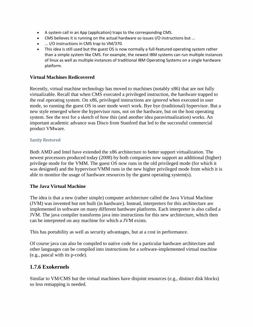
A system call in an App (application) traps to the corresponding CMS. CMS believes it is running on the actual hardware so issues I/O instructions but ... ... I/O instructions in CMS trap to VM/370. This idea is still used but the guest OS is now normally a full-featured operating system rather
than a simple system like CMS. For example, the newest IBM systems can run multiple instances of linux as well as multiple instances of traditional IBM Operating Systems on a single hardware platform.
Virtual Machines Redicovered
Recently, virtual machine technology has moved to machines (notably x86) that are not fully
virtualizable. Recall that when CMS executed a privileged instruction, the hardware trapped to
the real operating system. On x86, privileged instructions are ignored when executed in user
mode, so running the guest OS in user mode won't work. Bye bye (traditional) hypervisor. But a
new style emerged where the hypervisor runs, not on the hardware, but on the host operating
system. See the text for a sketch of how this (and another idea paravirtualization) works. An
important academic advance was Disco from Stanford that led to the successful commercial
product VMware.
Sanity Restored
Both AMD and Intel have extended the x86 architecture to better support virtualization. The
newest processors produced today (2008) by both companies now support an additional (higher)
privilege mode for the VMM. The guest OS now runs in the old privileged mode (for which it
was designed) and the hypervisor/VMM runs in the new higher privileged mode from which it is
able to monitor the usage of hardware resources by the guest operating system(s).
The Java Virtual Machine
The idea is that a new (rather simple) computer architecture called the Java Virtual Machine
(JVM) was invented but not built (in hardware). Instead, interpreters for this architecture are
implemented in software on many different hardware platforms. Each interpreter is also called a
JVM. The java compiler transforms java into instructions for this new architecture, which then
can be interpreted on any machine for which a JVM exists.
This has portability as well as security advantages, but at a cost in performance.
Of course java can also be compiled to native code for a particular hardware architecture and
other languages can be compiled into instructions for a software-implemented virtual machine
(e.g., pascal with its p-code).
1.7.6 Exokernels
Similar to VM/CMS but the virtual machines have disjoint resources (e.g., distinct disk blocks)
so less remapping is needed.
1.8 The World According to C
1.8.1 The C Language
Assumed knowledge.
1.8.2 Header Files
Assumed knowledge.
1.8.3 Large Programming Projects
Mostly assumed knowledge. Linker's are very briefly discussed. Our earlier discussion was much
more detailed.
1.8.4 The model of Run Time
Extremely brief treatment with only a few points made about the running of the operating itself.
The text (code) segment is normally read only. The stack is initially of size zero; it grows and shrinks as functions are called and return. The data segment is initially not empty, with some of it is initialized. It can grow under program
control and perhaps can shrink.
1.9 Research on Operating Systems
Skipped
1.10 Outline of the Rest of this Book
Skipped
1.11 Metric Units
Assumed knowledge. Note that what is covered is just the prefixes, i.e. the names and
abbreviations for various powers of 10.
1.12 Summary
Skipped, but you should read and be sure you understand it (about 2/3 of a page).
Chapter 2 Process and Thread Management
Tanenbaum's chapter title is Processes and Threads. I prefer to add the word management. The
subject matter is processes, threads, scheduling, interrupt handling, and IPC (InterProcess
Communication—and Coordination).
2.1 Processes
Definition: A process is a program in execution.
We are assuming a multiprogramming OS that can switch from one process to another. Sometimes this is called pseudoparallelism since one has the illusion of a parallel processor. The other possibility is real parallelism in which two or more processes are actually running at
once because the computer system is a parallel processor, i.e., has more than one processor. We do not study real parallelism (parallel processing, distributed systems, multiprocessors, etc)
in this course.
2.1.1 The Process Model
Even though in actuality there are many processes running at once, the OS gives each process the
illusion that it is running alone.
Virtual time: The time used by just this processes. Virtual time progresses at a rate independent of other processes. (Actually, this is false, the virtual time is typically incremented a little during the systems calls used for process switching; so if there are other processes, overhead virtual time occurs.)
Virtual memory: The memory as viewed by the process. Each process typically believes it has a contiguous chunk of memory starting at location zero. Of course this can't be true of all processes (or they would be using the same memory) and in modern systems it is actually true of no processes (the memory assigned to a single process is not contiguous and does not include location zero). Think of the individual modules that are input to the linker. Each numbers its addresses from zero; the linker eventually translates these relative addresses into absolute addresses. That is the linker provides to the assembler a virtual memory in which addresses start at zero.
Virtual time and virtual memory are examples of abstractions provided by the operating system
to the user processes so that the latter experiences a more pleasant virtual machine than actually
exists.
2.1.2 Process Creation
From the users' or external viewpoint there are several mechanisms for creating a process.
1. System initialization, including daemon (see below) processes. 2. Execution of a process creation system call by a running process. 3. A user request to create a new process. 4. Initiation of a batch job.
But looked at internally, from the system's viewpoint, the second method dominates. Indeed in
early Unix only one process is created at system initialization (the process is called init); all the
others are decendents of this first process.
Why have init? That is why not have all processes created via method 2?
Ans: Because without init there would be no running process to create any others.
Definition of Daemon
Many systems have daemon process lurking around to perform tasks when they are needed. I
was pretty sure the terminology was related to mythology, but didn't have a reference until a
daemon: /day'mn/ or /dee'mn/ n. [from the mythological meaning, later rationalized as the acronym
`Disk And Execution MONitor'] A program that is not invoked explicitly, but lies dormant waiting for
some condition(s) to occur. The idea is that the perpetrator of the condition need not be aware that a
daemon is lurking (though often a program will commit an action only because it knows that it will
implicitly invoke a daemon). For example, under {ITS}, writing a file on the LPT spooler's directory would
invoke the spooling daemon, which would then print the file. The advantage is that programs wanting
(in this example) files printed need neither compete for access to nor understand any idiosyncrasies of
the LPT. They simply enter their implicit requests and let the daemon decide what to do with them.
Daemons are usually spawned automatically by the system, and may either live forever or be
regenerated at intervals. Daemon and demon are often used interchangeably, but seem to have distinct
connotations. The term `daemon' was introduced to computing by CTSS people (who pronounced it
/dee'mon/) and used it to refer to what ITS called a dragon; the prototype was a program called
DAEMON that automatically made tape backups of the file system. Although the meaning and the
pronunciation have drifted, we think this glossary reflects current (2000) usage.
As is often the case, wikipedia.org proved useful. Here is the first paragraph of a more thorough
entry. The wikipedia also has entries for other uses of daemon.
In Unix and other computer multitasking operating systems, a daemon is a computer program that runs
in the background, rather than under the direct control of a user; they are usually instantiated as
processes. Typically daemons have names that end with the letter "d"; for example, syslogd is the
daemon which handles the system log.
2.1.3 Process Termination
Again from the outside there appear to be several termination mechanism.
1. Normal exit (voluntary). 2. Error exit (voluntary). 3. Fatal error (involuntary). 4. Killed by another process (involuntary).
And again, internally the situation is simpler. In Unix terminology, there are two system calls kill
and exit that are used. Kill (poorly named in my view) sends a signal to another process. If this
signal is not caught (via the signal system call) the process is terminated. There is also an
uncatchable signal. Exit is used for self termination and can indicate success or failure.
2.1.4 Process Hierarchies
Modern general purpose operating systems permit a user to create and destroy processes.
In unix this is done by the fork system call, which creates a child process, and the exit system call, which terminates the current process.
After a fork both parent and child keep running (indeed they have the same program text) and each can fork off other processes.
A process tree results. The root of the tree is a special process created by the OS during startup. A process can choose to wait for children to terminate. For example, if C issued a wait() system
call it would block until G finished.
Old or primitive operating system like MS-DOS are not fully multiprogrammed, so when one
process starts another, the first process is automatically blocked and waits until the second is
finished. This implies that the process tree degenerates into a line.
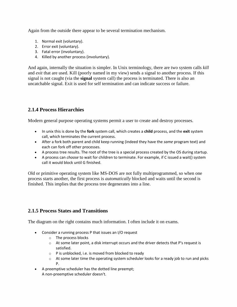
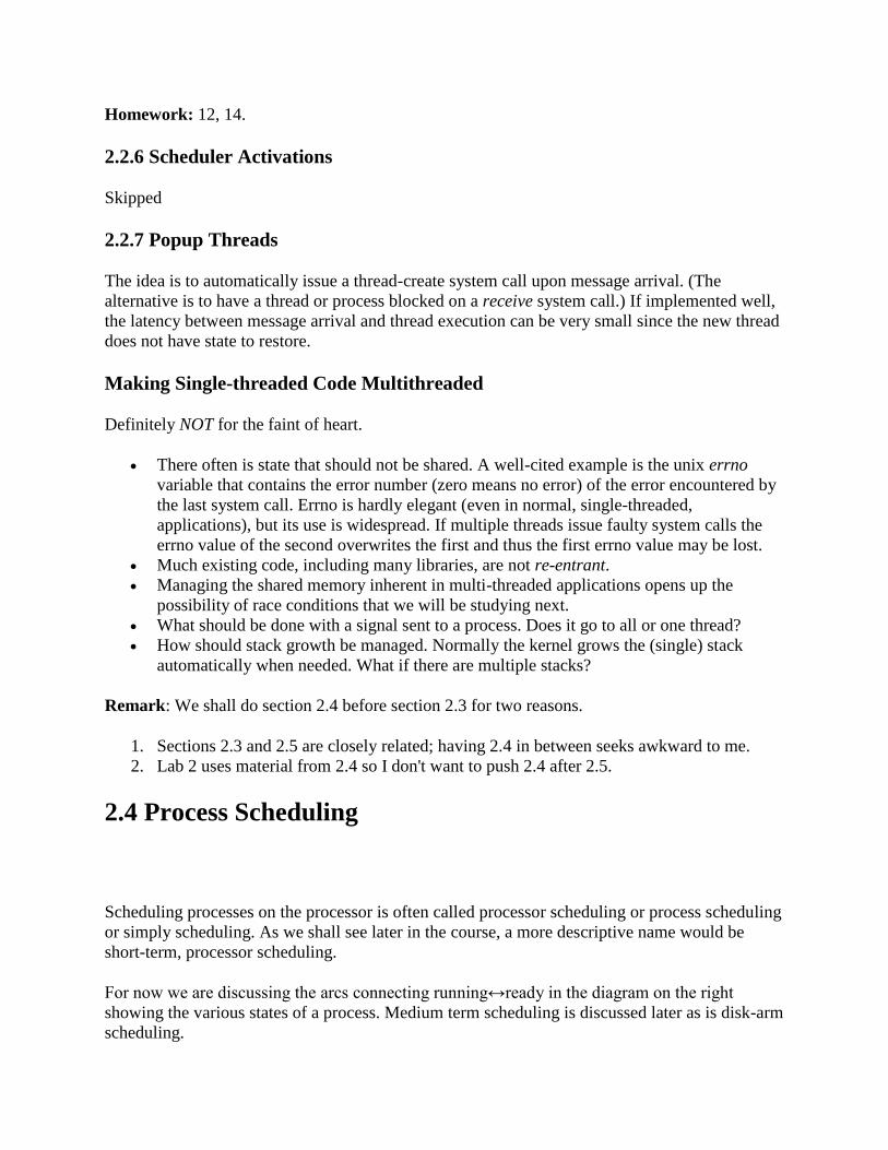
2.1.5 Process States and Transitions
The diagram on the right contains much information. I often include it on exams.
Consider a running process P that issues an I/O request o The process blocks o At some later point, a disk interrupt occurs and the driver detects that P's request is
satisfied. o P is unblocked, i.e. is moved from blocked to ready o At some later time the operating system scheduler looks for a ready job to run and picks
P. A preemptive scheduler has the dotted line preempt;
A non-preemptive scheduler doesn't.
The number of processes changes only for two arcs: create and terminate. Suspend and resume are medium term scheduling
o Done on a longer time scale. o Involves memory management as well. As a result we study it later. o Sometimes called two level scheduling.
Homework: 1.
One can organize an OS around the scheduler.
Write a minimal kernel (a micro-kernel) consisting of the scheduler, interrupt handlers, and IPC (interprocess communication).
The rest of the OS consists of kernel processes (e.g. memory, filesystem) that act as servers for the user processes (which of course act as clients).
The system processes also act as clients (of other system processes).
The above is called the client-server model and is one Tanenbaum likes. His Minix operating system works this way.
Indeed, there was reason to believe that the client-server model would dominate OS design. But that hasn't happened.
Such an OS is sometimes called server based.
Systems like traditional unix or linux would then be called self-service since the user process serves itself. That is, the user process switches to kernel mode (via the TRAP instruction) and performs the system call itself without transferring control to another process.
2.1.6 Implementation of Processes
The OS organizes the data about each process in a table naturally called the process table. Each
entry in this table is called a process table entry or process control block (PCB).
I have often referred to a process table entry as a PTE, but this is bad since I also use PTE for
Page Table Entry. Because the latter usage is very common, I must stop using PTE to abbreviate
the former. Please correct me if I slip up.
Characteristics of the process table.
One entry per process. The central data structure for process management. A process state transition (e.g., moving from blocked to ready) is reflected by a change in the
value of one or more fields in the PCB. We have converted an active entity (process) into a data structure (PCB). Finkel calls this the
level principle an active entity becomes a data structure when looked at from a lower level.
The PCB contains a great deal of information about the process. For example, o Saved value of registers including the program counter (i.e., the address of the next
instruction) when the process not running. o Stack pointer o CPU time used o Process id (PID) o Process id of parent (PPID) o User id (uid and euid) o Group id (gid and egid) o Pointer to text segment (memory for the program text) o Pointer to data segment o Pointer to stack segment o UMASK (default permissions for new files) o Current working directory o Many others
2.1.6A: An Addendum on Interrupts
This should be compared with the addenda on transfer of control and trap.
In a well defined location in memory (specified by the hardware) the OS stores an interrupt
vector, which contains the address of the interrupt handler.
Tanenbaum calls the interrupt handler the interrupt service routine. Actually one can have different priorities of interrupts and the interrupt vector then contains
one pointer for each level. This is why it is called a vector.
Assume a process P is running and a disk interrupt occurs for the completion of a disk read
previously issued by process Q, which is currently blocked. Note that disk interrupts are unlikely
to be for the currently running process (because the process that initiated the disk access is likely
blocked).
Actions by P Just Prior to the Interrupt:
1. Who knows?? This is the difficulty of debugging code depending on interrupts, the interrupt can occur (almost) anywhere. Thus, we do not know what happened just before the interrupt. Indeed, we do not even know which process P will be running when the interrupt does occur. We cannot (even for one specific execution) point to an instruction and say this instruction caused the interrupt.
Executing the interrupt itself:
2. The hardware saves the program counter and some other registers (or switches to using another set of registers, the exact mechanism is machine dependent).
3. The hardware loads new program counter from the interrupt vector.
o Loading the program counter causes a jump. o Steps 2 and 3 are similar to a procedure call. But the interrupt is asynchronous.
4. As with a trap, the hardware automatically switches the system into privileged mode. (It might have been in supervisor mode already. That is, an interrupt can occur in supervisor or user mode.)
Actions by the interrupt handler (et al) upon being activated
5. An assembly language routine saves registers.
6. The assembly routine sets up a new stack. (These last two steps are often called setting up the C environment.)
7. The assembly routine calls a procedure in a high level language, often the C language (Tanenbaum forgot this step).
8. The C procedure does the real work. o Determines what caused the interrupt (in this case a disk completed an I/O). o How does it figure out the cause?
It might know the priority of the interrupt being activated. The controller might write information in memory before the interrupt. The OS might read registers in the controller.
o Mark process Q as ready to run. That is move Q to the ready list (note that again we are viewing Q as a data
structure). Q is now in ready state; it was in the blocked state before. The code that Q needs to run initially is likely to be OS code. For example, the
data just read is probably now in kernel space and Q needs to copy it into user space.
o Now we have at least two processes ready to run, namely P and Q. There may be arbitrarily many others.
9. The scheduler decides which process to run, P or Q or something else. (This very loosely corresponds to g calling other procedures in the simple f calls g case we discussed previously). Eventually the scheduler decides to run P.
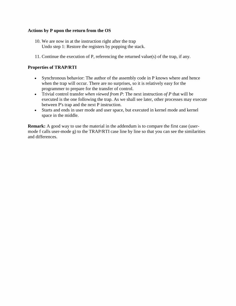
Actions by P when control returns
10. The C procedure (that did the real work in the interrupt processing) continues and returns to the assembly code.
11. Assembly language restores P's state (e.g., registers) and starts P at the point it was when the interrupt occurred.
Properties of interrupts
Phew. Unpredictable (to an extent). We cannot tell what was executed just before the interrupt
occurred. That is, the control transfer is asynchronous; it is difficult to ensure that everything is always prepared for the transfer.
The user code is unaware of the difficulty and cannot (easily) detect that it occurred. This is another example of the OS presenting the user with a virtual machine environment that is more pleasant than reality (in this case synchronous rather asynchronous behavior).
Interrupts can also occur when the OS itself is executing. This can cause difficulties since both the main line code and the interrupt handling code are from the same program, namely the OS, and hence might well be using the same variables. We will soon see how this can cause great problems even in what appear to be trivial cases.
The interprocess control transfer is neither stack-like nor queue-like. That is if first P was running, then Q was running, then R was running, then S was running, the next process to be run might be any of P, Q, or R (or some other process).
The system might have been in user-mode or supervisor mode when the interrupt occurred. The interrupt processing starts in supervisor mode.
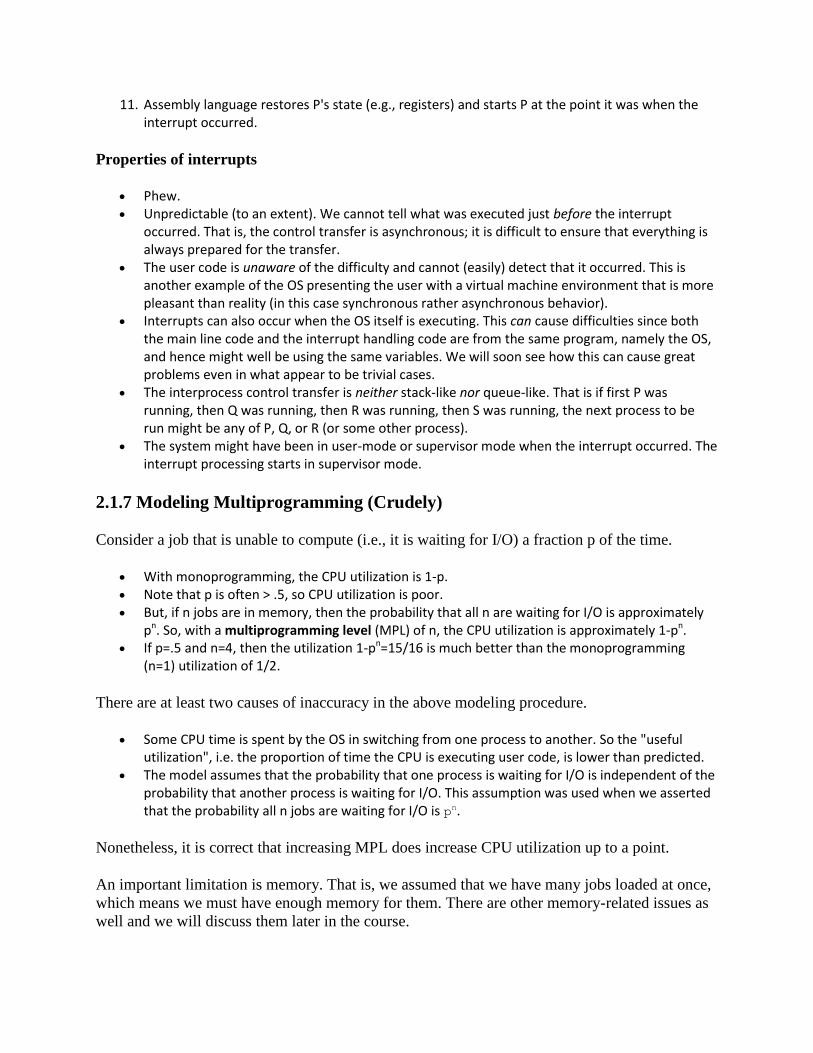
2.1.7 Modeling Multiprogramming (Crudely)
Consider a job that is unable to compute (i.e., it is waiting for I/O) a fraction p of the time.
With monoprogramming, the CPU utilization is 1-p. Note that p is often > .5, so CPU utilization is poor. But, if n jobs are in memory, then the probability that all n are waiting for I/O is approximately
pn. So, with a multiprogramming level (MPL) of n, the CPU utilization is approximately 1-pn. If p=.5 and n=4, then the utilization 1-pn=15/16 is much better than the monoprogramming
(n=1) utilization of 1/2.
There are at least two causes of inaccuracy in the above modeling procedure.
Some CPU time is spent by the OS in switching from one process to another. So the "useful utilization", i.e. the proportion of time the CPU is executing user code, is lower than predicted.
The model assumes that the probability that one process is waiting for I/O is independent of the probability that another process is waiting for I/O. This assumption was used when we asserted that the probability all n jobs are waiting for I/O is pn.
Nonetheless, it is correct that increasing MPL does increase CPU utilization up to a point.
An important limitation is memory. That is, we assumed that we have many jobs loaded at once,
which means we must have enough memory for them. There are other memory-related issues as
well and we will discuss them later in the course.
Homework: 5.
2.2 Threads
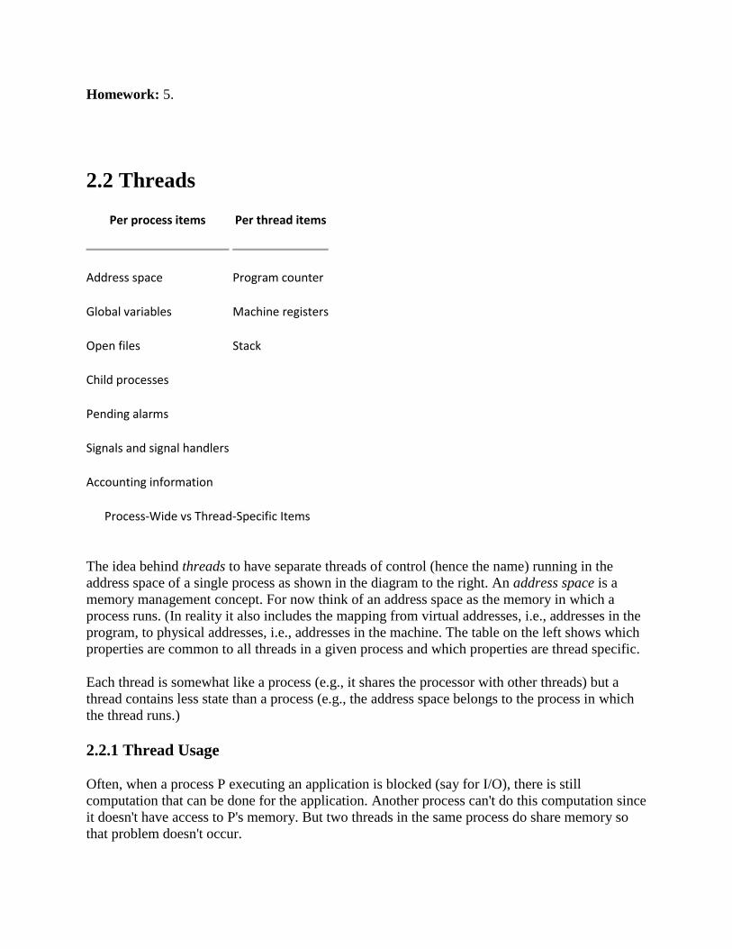
Per process items Per thread items
Address space Program counter
Global variables Machine registers
Open files Stack
Child processes
Pending alarms
Signals and signal handlers
Accounting information
Process-Wide vs Thread-Specific Items
The idea behind threads to have separate threads of control (hence the name) running in the
address space of a single process as shown in the diagram to the right. An address space is a
memory management concept. For now think of an address space as the memory in which a
process runs. (In reality it also includes the mapping from virtual addresses, i.e., addresses in the
program, to physical addresses, i.e., addresses in the machine. The table on the left shows which
properties are common to all threads in a given process and which properties are thread specific.
Each thread is somewhat like a process (e.g., it shares the processor with other threads) but a
thread contains less state than a process (e.g., the address space belongs to the process in which
the thread runs.)
2.2.1 Thread Usage
Often, when a process P executing an application is blocked (say for I/O), there is still
computation that can be done for the application. Another process can't do this computation since
it doesn't have access to P's memory. But two threads in the same process do share memory so
that problem doesn't occur.
An important modern example is a multithreaded web server. Each thread is responding to a
single WWW connection. While one thread is blocked on I/O, another thread can be processing
another WWW connection.
Question: Why not use separate processes, i.e., what is the shared memory?
Answer: The cache of frequently referenced pages.
A common organization for a multithreaded application is to have a dispatcher thread that fields
requests and then passes each request on to an idle worker thread. Since the dispatcher and
worker share memory, passing the request is very low overhead.
Another example is a producer-consumer problem (see below) in which we have 3 threads in a
pipeline. One thread reads data from an I/O device into an input buffer, the second thread
performs computation on the input buffer and places results in an output buffer, and the third
thread outputs the data found in the output buffer. Again, while one thread is blocked the others
can execute.
Really you want 2 (or more) input buffers and 2 (or more) output buffers. Otherwise the middle
thread would be using all the buffers and would block both outer threads.
Question: When does each thread block?
Answer:
1. The first thread blocks while waiting for the device to supply the data. It also blocks if all input buffers for the computational thread are full.
2. The second thread blocks when either all input buffers are empty or all output buffers are full. 3. The third thread blocks while waiting for the device to complete the output (or at least indicate
that it is ready for another request). It also blocks if all output buffers are empty.
A final (related) example is that an application wishing to perform automatic backups can have a
thread to do just this. In this way the thread that interfaces with the user is not blocked during the
backup. However some coordination between threads may be needed so that the backup is of a
Should its priority be frozen during the blockage. Let us assume the first case (reset to zero)
since it seems the simplest.
Approximating the Behavior of SFJ and PSJF
Recall that SFJ/PSFJ do a good job of minimizing the average waiting time. The problem with
them is the difficulty in finding the job whose next CPU burst is minimal. We now learn three
scheduling algorithms that attempt to do this. The first algorithm does it statically, presumably
with some manual help; the other two are dynamic and fully automatic.
Multilevel Queues (**, **, MLQ, **)
Put different classes of processs in different queues
Processes do not move from one queue to another.
Can have different policies on the different queues.
For example, might have a background (batch) queue that is FCFS and one or more
foreground queues that are RR (possibly with different quanta).
Must also have a policy among the queues.
For example, might have two queues, foreground and background, and give the first
absolute priority over the second
o Might apply priority aging to prevent background starvation.
o But might not, i.e., no guarantee of service for background processes. View a
background process as a cycle soaker.
o Might have 3 queues, foreground, background, cycle soaker.
Another possible inter-queue policy would be have 2 queues, apply RR to each but cycle
through the higher priority twice and then cycle through the lower priority queue once.
Multiple Queues (FB, MFQ, MLFBQ, MQ)
As with multilevel queues above we have many queues, but now processes move from queue to
queue in an attempt to dynamically separate batch-like from interactive processs so that we can
favor the latter.
Remember that low average waiting time is achieved by SJF and this is an attempt to
determine dynamically those processes that are interactive, which means have a very
short cpu burst.
Run processs from the highest priority nonempty queue in a RR manner.
When a process uses its full quanta (looks a like batch process), move it to a lower
priority queue.
When a process doesn't use a full quanta (looks like an interactive process), move it to a
higher priority queue.
A long process with frequent (perhaps spurious) I/O will remain in the upper queues.
Might have the bottom queue FCFS.
Many variants.
For example, might let process stay in top queue 1 quantum, next queue 2 quanta, next
queue 4 quanta (i.e., sometimes return a process to the rear of the same queue it was in if
the quantum expires).
Might move to a higher queue only if a keyboard interrupt occurred rather than if the
quantum failed to expire for any reason (e.g., disk I/O).
Shortest Process Next
An attempt to apply sjf to interactive scheduling. What is needed is an estimate of how long the
process will run until it blocks again. One method is to choose some initial estimate when the
process starts and then, whenever the process blocks choose a new estimate via
NewEstimate = A*OldEstimate + (1-A)*LastBurst
where 0<A<1 and LastBurst is the actual time used during the burst that just ended.
Highest Penalty Ratio Next (HPRN, HRN, **, **)
Run the process that has been hurt the most.
For each process, let r = T/t; where T is the wall clock time this process has been in
system and t is the running time of the process to date.
If r=2.5, that means the job has been running 1/2.5 = 40% of the time it has been in the
system.
We call r the penalty ratio and run the process having the highest r value.
We must worry about a process that just enters the system since t=0 and hence the ratio is
undefined. Define t to be the max of 1 and the running time to date. Since now t is at least
1, the ratio is always defined.
HPRN is normally defined to be non-preemptive (i.e., the system only checks r when a
burst ends), but there is an preemptive analogue
o When putting a process into the run state compute the time at which it will no
longer have the highest ratio and set a timer.
o When a process is moved into the ready state, compute its ratio and preempt if
needed.
HRN stands for highest response ratio next and means the same thing.
This policy is yet another example of priority scheduling
Guaranteed Scheduling
A variation on HPRN. The penalty ratio is a little different. It is nearly the reciprocal of the
above, namely t / (T/n)
where n is the multiprogramming level. So if n is constant, this ratio is a constant times 1/r.
Lottery Scheduling
Each process gets a fixed number of tickets and at each scheduling event a random ticket is
drawn (with replacement) and the process holding that ticket runs for the next interval (probably
a RR-like quantum q).
On the average a process with P percent of the tickets will get P percent of the CPU (assuming
no blocking, i.e., full quanta).
Fair-Share Scheduling
If you treat processes fairly you may not be treating users fairly since users with many processes
will get more service than users with few processes. The scheduler can group processes by user
and only give one of a user's processes a time slice before moving to another user.
Fancier methods have been implemented that give some fairness to groups of users. Say one
group paid 30% of the cost of the computer. That group would be entitled to 30% of the cpu
cycles providing it had at least one process active. Furthermore a group earns some credit when
it has no processes active.
Theoretical Issues
Considerable theory has been developed.
NP completeness results abound.
Much work in queuing theory to predict performance.
Not covered in this course.
Medium-Term Scheduling
In addition to the short-term scheduling we have discussed, we add medium-term scheduling in
which decisions are made at a coarser time scale.
Recall my favorite diagram, shown again on the right. Medium term scheduling determines the
transitions from the top triangle to the bottom line. We suspend (swap out) some process if
memory is over-committed dropping the (ready or blocked) process down. We also need resume
transitions to return a process to the top triangle.
Criteria for choosing a victim to suspend include:
How long since previously suspended.
How much CPU time used recently.
How much memory does it use.
External priority (pay more, get swapped out less).
We will discuss medium term scheduling again when we study memory management.
Long Term Scheduling
This is sometimes called Job scheduling.
1. The system decides when to start jobs, i.e., it does not necessarily start them when
submitted.
2. Used at many supercomputer sites.
A similar idea (but more drastic and not always so well coordinated) is to force some users to log
out, kill processes, and/or block logins if over-committed.
CTSS (an early time sharing system at MIT) did this to insure decent interactive response
time.
Unix does this if out of memory.
LEM jobs during the day (Grumman).
2.4.4 Scheduling in Real Time Systems
Skipped
2.4.5 Policy versus Mechanism
Skipped.
2.4.6 Thread Scheduling
Skipped.
Review Homework Assigned Last Time
Lab 2 (Scheduling) Discussion
Show the detailed output
1. In FCFS see the affect of A, B, C, and I/O
2. In RR see how the cpu burst is limited.
3. Note the intital sorting to ease finding the tie breaking process.
4. Note show random.
5. Comment on how to do it: (time-based) discrete-event simulation (DES).
i. DoBlockedProcesses()
ii. DoRunningProcesses()
iii. DoCreatedProcesses()
iv. DoReadyProcesses()
6. For processor sharing need event-based DES.
Operating Systems
Start Lecture #6
2.3 Interprocess Communication (IPC) and
Coordination/Synchronization
2.3.1 Race Conditions
A race condition occurs when two (or more) processes are about to perform some action.
Depending on the exact timing, one or other goes first. If one of the processes goes first,
everything works correctly, but if another one goes first, an error, possibly fatal, occurs.
Imagine two processes both accessing x, which is initially 10.
A1: LOAD r1,x B1: LOAD r2,x
A2: ADD r1,1 B2: SUB r2,1
A3: STORE r1,x B3: STORE r2,x
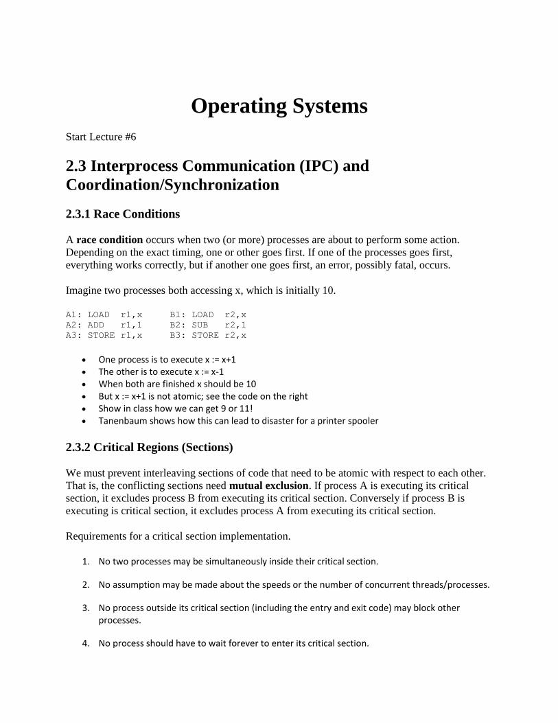
One process is to execute x := x+1 The other is to execute x := x-1 When both are finished x should be 10 But x := x+1 is not atomic; see the code on the right Show in class how we can get 9 or 11! Tanenbaum shows how this can lead to disaster for a printer spooler
2.3.2 Critical Regions (Sections)
We must prevent interleaving sections of code that need to be atomic with respect to each other.
That is, the conflicting sections need mutual exclusion. If process A is executing its critical
section, it excludes process B from executing its critical section. Conversely if process B is
executing is critical section, it excludes process A from executing its critical section.
Requirements for a critical section implementation.
1. No two processes may be simultaneously inside their critical section.
2. No assumption may be made about the speeds or the number of concurrent threads/processes.
3. No process outside its critical section (including the entry and exit code) may block other processes.
4. No process should have to wait forever to enter its critical section.
o I do NOT make this last requirement. o I just require that the system as a whole make progress (so not all processes are
blocked). o I refer to solutions that do not satisfy Tanenbaum's last condition as unfair, but
nonetheless correct, solutions. o Stronger fairness conditions have also been defined.
2.3.3 Mutual exclusion with busy waiting
We will study only solutions in this class. Note that higher level solutions, e.g., having one
process block when it cannot enter its critical are implemented using busy waiting algorithms.
Disabling Interrupts
The operating system can choose not to preempt itself. That is, we could choose not to preempt
system processes (if the OS is client server) or processes running in system mode (if the OS is
self service). Forbidding preemption for system processes would prevent the problem above
where x<--x+1 not being atomic crashed the printer spooler if the spooler is part of the OS.
The way to prevent preemption of kernel-mode code is to disable interrupts. Indeed, disabling
(i.e., temporarily preventing) interrupts is often done for exactly this reason.
This is not, however, sufficient for all cases.
It does not work for user-mode programs. So the Unix print spooler, which is a user-mode program would need another solution.
We do not want to block interrupts for too long or the system will seem unresponsive. Disabling interrupts is insufficient if the system has several processors.
o The main line can be executing on both processors simultaneously so interrupts are not involved.
o One processor cannot block interrupts on the other.
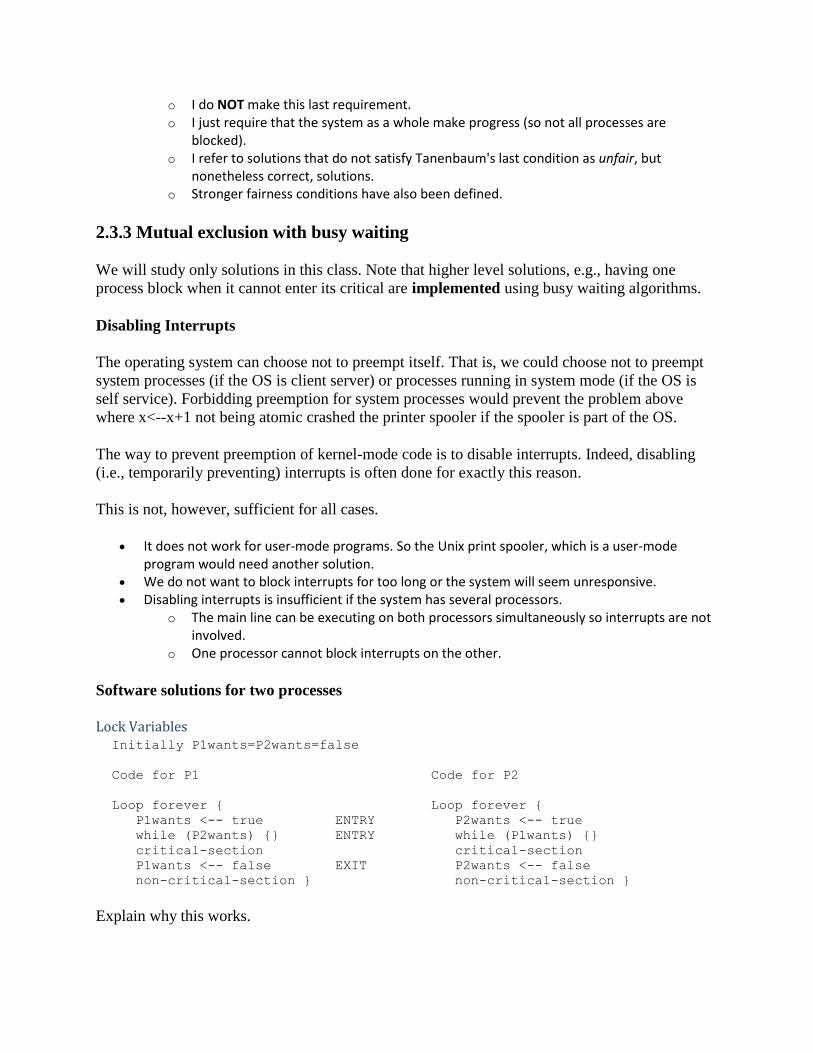
Software solutions for two processes
Lock Variables Initially P1wants=P2wants=false
Code for P1 Code for P2
Loop forever { Loop forever {
P1wants <-- true ENTRY P2wants <-- true
while (P2wants) {} ENTRY while (P1wants) {}
critical-section critical-section
P1wants <-- false EXIT P2wants <-- false
non-critical-section } non-critical-section }
Explain why this works.
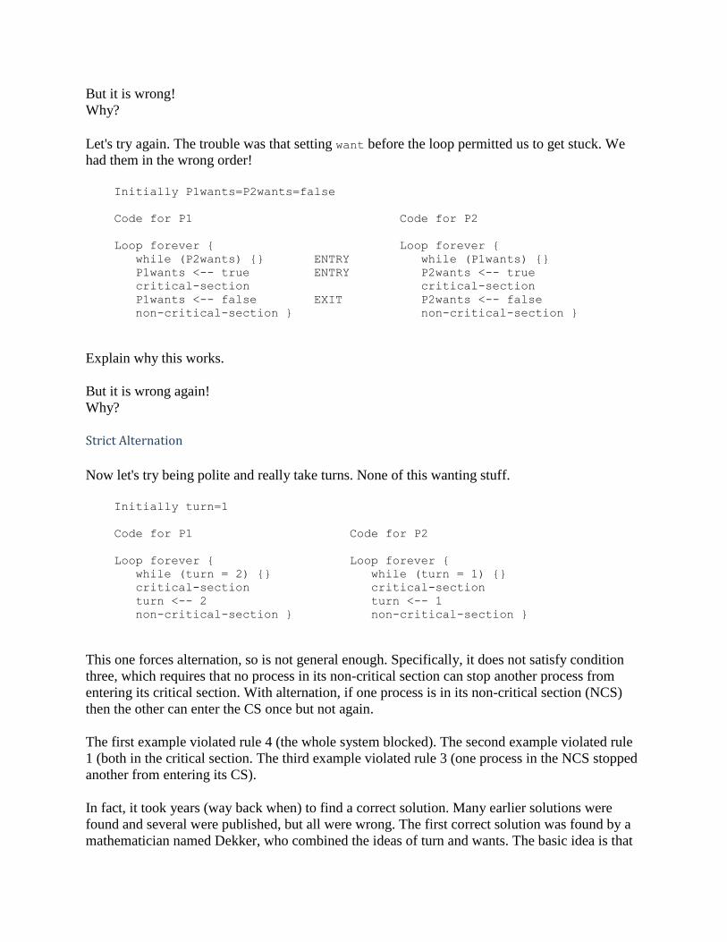
But it is wrong!
Why?
Let's try again. The trouble was that setting want before the loop permitted us to get stuck. We
had them in the wrong order!
Initially P1wants=P2wants=false
Code for P1 Code for P2
Loop forever { Loop forever {
while (P2wants) {} ENTRY while (P1wants) {}
P1wants <-- true ENTRY P2wants <-- true
critical-section critical-section
P1wants <-- false EXIT P2wants <-- false
non-critical-section } non-critical-section }
Explain why this works.
But it is wrong again!
Why?
Strict Alternation
Now let's try being polite and really take turns. None of this wanting stuff.
Initially turn=1
Code for P1 Code for P2
Loop forever { Loop forever {
while (turn = 2) {} while (turn = 1) {}
critical-section critical-section
turn <-- 2 turn <-- 1
non-critical-section } non-critical-section }
This one forces alternation, so is not general enough. Specifically, it does not satisfy condition
three, which requires that no process in its non-critical section can stop another process from
entering its critical section. With alternation, if one process is in its non-critical section (NCS)
then the other can enter the CS once but not again.
The first example violated rule 4 (the whole system blocked). The second example violated rule
1 (both in the critical section. The third example violated rule 3 (one process in the NCS stopped
another from entering its CS).
In fact, it took years (way back when) to find a correct solution. Many earlier solutions were
found and several were published, but all were wrong. The first correct solution was found by a
mathematician named Dekker, who combined the ideas of turn and wants. The basic idea is that
you take turns when there is contention, but when there is no contention, the requesting process
can enter. It is very clever, but I am skipping it (I cover it when I teach distributed operating
systems in V22.0480 or G22.2251). Subsequently, algorithms with better fairness properties
were found (e.g., no task has to wait for another task to enter the CS twice).
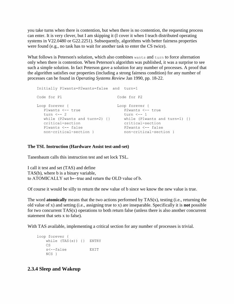
What follows is Peterson's solution, which also combines wants and turn to force alternation
only when there is contention. When Peterson's algorithm was published, it was a surprise to see
such a simple solution. In fact Peterson gave a solution for any number of processes. A proof that
the algorithm satisfies our properties (including a strong fairness condition) for any number of
processes can be found in Operating Systems Review Jan 1990, pp. 18-22.
Initially P1wants=P2wants=false and turn=1
Code for P1 Code for P2
Loop forever { Loop forever {
P1wants <-- true P2wants <-- true
turn <-- 2 turn <-- 1
while (P2wants and turn=2) {} while (P1wants and turn=1) {}
critical-section critical-section
P1wants <-- false P2wants <-- false
non-critical-section } non-critical-section }
The TSL Instruction (Hardware Assist test-and-set)
Tanenbaum calls this instruction test and set lock TSL.
I call it test and set (TAS) and define
TAS(b), where b is a binary variable,
to ATOMICALLY set b←true and return the OLD value of b.
Of course it would be silly to return the new value of b since we know the new value is true.
The word atomically means that the two actions performed by TAS(x), testing (i.e., returning the
old value of x) and setting (i.e., assigning true to x) are inseparable. Specifically it is not possible
for two concurrent TAS(x) operations to both return false (unless there is also another concurrent
statement that sets x to false).
With TAS available, implementing a critical section for any number of processes is trivial.
loop forever {
while (TAS(s)) {} ENTRY
CS
s<--false EXIT
NCS }
2.3.4 Sleep and Wakeup
Remark: Tanenbaum presents both busy waiting (as above) and blocking (process switching)
solutions. We present only do busy waiting solutions, which are easier and used in the blocking
solutions. Sleep and Wakeup are the simplest blocking primitives. Sleep voluntarily blocks the
process and wakeup unblocks a sleeping process. However, it is far from clear how sleep and
wakeup are implemented. Indeed, deep inside, they typically use TAS or some similar primitive.
We will not cover these solutions.
Homework: Explain the difference between busy waiting and blocking process synchronization.
2.3.5: Semaphores
Remark: Tannenbaum use the term semaphore only for blocking solutions. I will use the term
for our busy waiting solutions (as well as for blocking solutions). Others call our solutions spin
locks.
P and V and Semaphores
The entry code is often called P and the exit code V. Thus the critical section problem is to write
P and V so that
loop forever
P
critical-section
V
non-critical-section
satisfies
1. Mutual exclusion. 2. No speed assumptions. 3. No blocking by processes in NCS. 4. Forward progress (my weakened version of Tanenbaum's last condition).
Note that I use indenting carefully and hence do not need (and sometimes omit) the braces {}
used in languages like C or java.
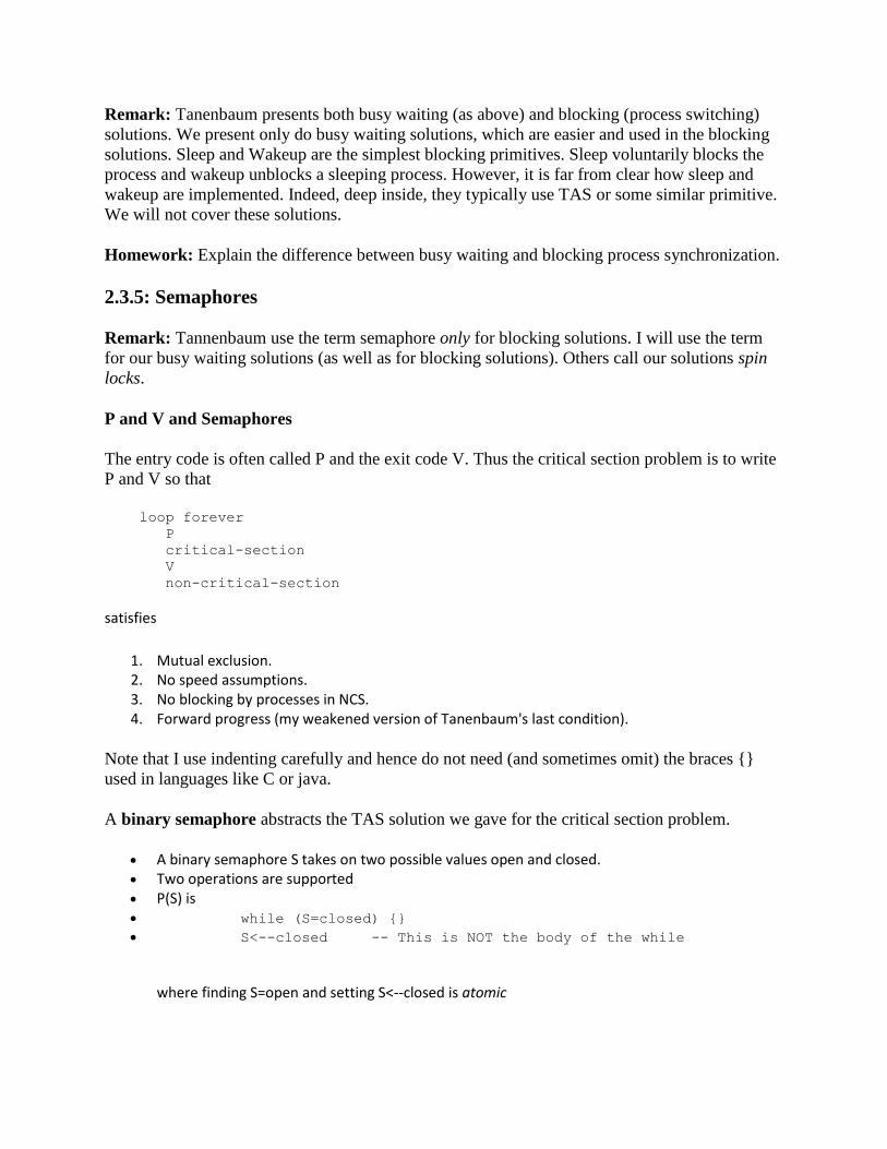
A binary semaphore abstracts the TAS solution we gave for the critical section problem.
A binary semaphore S takes on two possible values open and closed. Two operations are supported P(S) is while (S=closed) {}
S<--closed -- This is NOT the body of the while
where finding S=open and setting S<--closed is atomic
That is, wait until the gate is open, then run through and atomically close the gate Said another way, it is not possible for two processes doing P(S) simultaneously to both see
S=open (unless a V(S) is also simultaneous with both of them). V(S) is simply S<--open
The above code is not real, i.e., it is not an implementation of P. It requires a sequence of two
instructions to be atomic and that is, after all, what we are trying to implement in the first place.
The above code is, instead, a definition of the effect P is to have.
To repeat: for any number of processes, the critical section problem can be solved by
loop forever
P(S)
CS
V(S)
NCS
The only solution we have seen for an arbitrary number of processes is the one just above with
P(S) implemented via test and set.
Remark: Peterson's solution requires each process to know its process number; the TAS soluton
does not. Moreover the definition of P and V does not permit use of the process number. Thus,
strictly speaking Peterson did not provide an implementation of P and V. He did solve the critical
section problem.
To solve other coordination problems we want to extend binary semaphores.
With binary semaphores, two consecutive Vs do not permit two subsequent Ps to succeed (the gate cannot be doubly opened).
We might want to limit the number of processes in the section to 3 or 4, not always just 1.
Both of the shortcomings can be overcome by not restricting ourselves to a binary variable, but
instead define a generalized or counting semaphore.
A counting semaphore S takes on non-negative integer values Two operations are supported P(S) is while (S=0) {}
S--
where finding S>0 and decrementing S is atomic
That is, wait until the gate is open (positive), then run through and atomically close the gate one unit
Another way to describe this atomicity is to say that it is not possible for the decrement to occur when S=0 and it is also not possible for two processes executing P(S) simultaneously to both see the same necessarily (positive) value of S unless a V(S) is also simultaneous.
V(S) is simply S++
Counting semaphores can solve what I call the semi-critical-section problem, where you premit
up to k processes in the section. When k=1 we have the original critical-section problem.
initially S=k
loop forever
P(S)
SCS -- semi-critical-section
V(S)
NCS
Solving the Producer-Consumer Problem Using Semaphores
Note that my definition of semaphore is different from Tanenbaum's so it is not surprising that
my solution is also different from his.
Unlike the previous problems of mutual exclusion, the producer-consumer has two classes of
processes
Producers, which produce times and insert them into a buffer. Consumers, which remove items and consume them.
What happens if the producer encounters a full buffer?
Answer: It waits for the buffer to become non-full.
What if the consumer encounters an empty buffer?
Answer: It waits for the buffer to become non-empty.
The producer-consumer problem is also called the bounded buffer problem, which is another
example of active entities being replaced by a data structure when viewed at a lower level
2.5.0 The Producer-Consumer (or Bounded Buffer) Problem
We did this previously.
2.5.1 The Dining Philosophers Problem
A classical problem from Dijkstra
5 philosophers sitting at a round table Each has a plate of spaghetti There is a fork between each two Need two forks to eat
What algorithm do you use for access to the shared resource (the forks)?
The obvious solution (pick up right; pick up left) deadlocks. Big lock around everything serializes. Good code in the book.
The purpose of mentioning the Dining Philosophers problem without giving the solution is to
give a feel of what coordination problems are like. The book gives others as well. The solutions
would be covered in a sequel course. If you are interested look, for example here.
Homework: 45 and 46 (these have short answers but are not easy). Note that the second problem
refers to fig. 2-20, which is incorrect. It should be fig 2-46.
2.5.2 The Readers and Writers Problem
As in the producer-consumer problem we have two classes of processes.
Readers, which can work concurrently. Writers, which need exclusive access.
The problem is to
1. prevent 2 writers from being concurrent. 2. prevent a reader and a writer from being concurrent. 3. permit readers to be concurrent when no writer is active. 4. (perhaps) insure fairness (e.g., freedom from starvation).
Solutions to the readers-writers problem are quite useful in multiprocessor operating systems and
database systems. The easy way out is to treat all processes as writers in which case the problem
reduces to mutual exclusion (P and V). The disadvantage of the easy way out is that you give up
reader concurrency. Again for more information see the web page referenced above.
2.5A Critical Sections versus Database Transactions
Critical Sections have a form of atomicity, in some ways similar to transactions. But there is a
key difference: With critical sections you have certain blocks of code, say A, B, and C, that are
mutually exclusive (i.e., are atomic with respect to each other) and other blocks, say D and E,
that are mutually exclusive; but blocks from different critical sections, say A and D, are not
mutually exclusive.
The day after giving this lecture in 2006-07-spring, I found a modern reference to the same
question. The quote below is from Subtleties of Transactional Memory Atomicity Semantics by
Blundell, Lewis, and Martin in Computer Architecture Letters (volume 5, number 2, July-Dec.
2006, pp. 65-66). As mentioned above, busy-waiting (binary) semaphores are often called locks
(or spin locks).
... conversion (of a critical section to a transaction) broadens the scope of atomicity, thus changing the
program's semantics: a critical section that was previously atomic only with respect to other critical
sections guarded by the same lock is now atomic with respect to all other critical sections.
2.5B: Summary of 2.3 and 2.5
We began with a subtle bug (wrong answer for x++ and x--) and used it to motivate the Critical
Section Problem for which we provided a (software) solution.
We then defined (binary) Semaphores and showed that a Semaphore easily solves the critical
section problem and doesn't require knowledge of how many processes are competing for the
critical section. We gave an implementation using Test-and-Set.
We then gave an operational definition of Semaphore (which is not an implementation) and
morphed this definition to obtain a Counting (or Generalized) Semaphore, for which we gave
NO implementation. I asserted that a counting semaphore can be implemented using 2 binary
semaphores and gave a reference.
We defined the Producer-Consumer (or Bounded Buffer) Problem and showed that it can be
solved using counting semaphores (and binary semaphores, which are a special case).
Finally we briefly discussed some classical problems, but did not give (full) solutions.
2.6 Research on Processes and Threads
Skipped.
2.7 Summary
Skipped, but you should read.
Chapter 6 Deadlocks
Remark: Deadlocks are closely related to process management so belong here, right after
chapter 2. It was here in 2e. A goal of 3e is to make sure that the basic material gets covered in
one semester. But I know we will do the first 6 chapters so there is no need for us to postpone the
study of deadlock.
A deadlock occurs when every member of a set of processes is waiting for an event that can only
be caused by a member of the set.
Often the event waited for is the release of a resource.
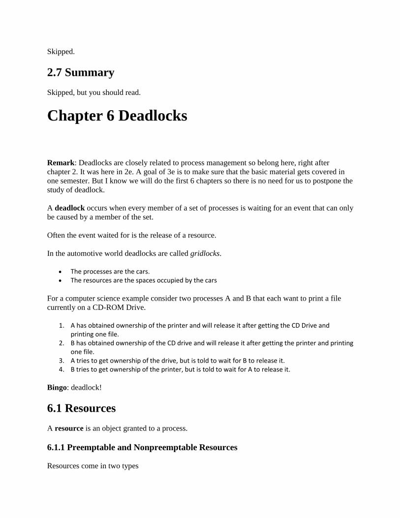
In the automotive world deadlocks are called gridlocks.
The processes are the cars. The resources are the spaces occupied by the cars
For a computer science example consider two processes A and B that each want to print a file
currently on a CD-ROM Drive.
1. A has obtained ownership of the printer and will release it after getting the CD Drive and printing one file.
2. B has obtained ownership of the CD drive and will release it after getting the printer and printing one file.
3. A tries to get ownership of the drive, but is told to wait for B to release it. 4. B tries to get ownership of the printer, but is told to wait for A to release it.
Bingo: deadlock!
6.1 Resources
A resource is an object granted to a process.
6.1.1 Preemptable and Nonpreemptable Resources
Resources come in two types
1. Preemptable, meaning that the resource can be taken away from its current owner (and given back later). An example is memory.
2. Non-preemptable, meaning that the resource cannot be taken away. An example is a printer.
The interesting issues arise with non-preemptable resources so those are the ones we study.
The life history of a resource is a sequence of
1. Request 2. Allocate 3. Use 4. Release
Processes request the resource, use the resource, and release the resource. The allocate decisions
are made by the system and we will study policies used to make these decisions.
6.1.2 Resource Acquisition
A simple example of the trouble you can get into.
Two resources and two processes. Each process wants both resources. Use a semaphore for each. Call them S and T. If both processes execute
P(S); P(T); --- V(T); V(S) all is well.
But if one executes instead P(T); P(S); -- V(S); V(T) disaster! This was the printer/CD example just above.
Recall from the semaphore/critical-section treatment last chapter, that it is easy to cause trouble
if a process dies or stays forever inside its critical section. We assume processes do not do this.
Similarly, we assume that no process retains a resource forever. It may obtain the resource an
unbounded number of times (i.e. it can have a loop forever with a resource request inside), but
each time it gets the resource, it must release it eventually.
6.2 Introduction to Deadlocks
Definition: A deadlock occurs when a every member of a set of processes is waiting for an event
that can only be caused by a member of the set.
Often the event waited for is the release of a resource.
6.2.1 (Necessary) Conditions for Deadlock
The following four conditions (Coffman; Havender) are necessary but not sufficient for
deadlock. Repeat: They are not sufficient.
1. Mutual exclusion: A resource can be assigned to at most one process at a time (no sharing). 2. Hold and wait: A processing holding a resource is permitted to request another. 3. No preemption: A process must release its resources; they cannot be taken away. 4. Circular wait: There must be a chain of processes such that each member of the chain is waiting
for a resource held by the next member of the chain.
One can say If you want a deadlock, you must have these four conditions.. But of course you
don't actually want a deadlock, so you would more likely say If you want to prevent deadlock,
you need only violate one or more of these four conditions..
The first three are static characteristics of the system and resources. That is, for a given system
with a fixed set of resources, the first three conditions are either always true or always false:
They don't change with time. The truth or falsehood of the last condition does indeed change
with time as the resources are requested/allocated/released.
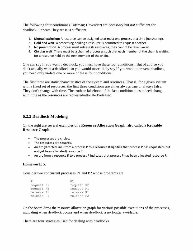
6.2.2 Deadlock Modeling
On the right are several examples of a Resource Allocation Graph, also called a Reusable
Resource Graph.
The processes are circles. The resources are squares. An arc (directed line) from a process P to a resource R signifies that process P has requested (but
not yet been allocated) resource R. An arc from a resource R to a process P indicates that process P has been allocated resource R.
Homework: 5.
Consider two concurrent processes P1 and P2 whose programs are.
P1 P2
request R1 request R2
request R2 request R1
release R2 release R1
release R1 release R2
On the board draw the resource allocation graph for various possible executions of the processes,
indicating when deadlock occurs and when deadlock is no longer avoidable.
There are four strategies used for dealing with deadlocks.
1. Ignore the problem 2. Detect deadlocks and recover from them 3. Prevent deadlocks by violating one of the 4 necessary conditions. 4. Avoid deadlocks by carefully deciding when to allocate resources.
6.3 Ignoring the problem—The Ostrich Algorithm
The put your head in the sand approach.
If the likelihood of a deadlock is sufficiently small and the cost of avoiding a deadlock is sufficiently high it might be better to ignore the problem. For example, if each PC deadlocks once per 10 years, the one reboot may be less painful that the restrictions needed to prevent it.
Clearly not a good philosophy for nuclear missile launchers or patient monitoring systems for cardiac care units.
For embedded systems (such as the two examples above) the programs run are fixed in advance so many of the issues that occur in systems like linux or windows (such as many processes wanting to fork at the same time) don't occur.
Operating Systems
Start Lecture #7
6.4 Detecting Deadlocks and Recovering From Them
6.4.1 Detecting Deadlocks with Single Unit Resources
Consider the case in which there is only one instance of each resource.
Thus a request can be satisfied by only one specific resource.
In this case the 4 necessary conditions for deadlock are also sufficient.
Remember we are making an assumption (single unit resources) that is often invalid. For
example, many systems have several printers and a request is given for a printer not a
specific printer. Similarly, one can have many CD-ROM drives.
So the problem comes down to finding a directed cycle in the resource allocation graph.
Why?
Answer: Because the other three conditions are either satisfied by the system we are
studying, or are not in which case deadlock is not a question. That is, conditions 1,2,3 are
static conditions on the system in general not conditions on the state of the system right
now.
To find a directed cycle in a directed graph is not hard. The algorithm is in the book. The idea is
simple.
1. For each node in the graph do a depth first traversal to see if the graph is a DAG (directed
acyclic graph), building a list as you go down the DAG (and pruning it as you backtrack
back up).
2. If you ever find the same node twice on your list, you have found a directed cycle, the
graph is not a DAG, and deadlock exists among the processes in your current list.
3. If you never find the same node twice, the graph is a DAG and no deadlock exists (right
now).
The searches are finite since there are a finite number of nodes.
6.4.2 Detecting Deadlocks with Multiple Unit Resources
This is more difficult.
The figure on the right shows a resource allocation graph with multiple unit resources.
Each unit is represented by a dot in the box.
Request edges are drawn to the box since they represent a request for any dot in the box.
Allocation edges are drawn from the dot to represent that this unit of the resource has
been assigned (but all units of a resource are equivalent and the choice of which one to
assign is arbitrary).
Note that there is a directed cycle in red, but there is no deadlock. Indeed the middle
process might finish, erasing the green arc and permitting the blue dot to satisfy the
rightmost process.
The book gives an algorithm for detecting deadlocks in this more general setting. The
idea is as follows.
1. look for a process that might be able to terminate. That is, a process all of whose
request arcs can be satisfied by resources the manager has on hand right now.
2. If one is found, pretend that it does terminate (erase all its arcs), and repeat step 1.
3. If any processes remain, they are deadlocked.
We will soon do in detail an algorithm (the Banker's algorithm) that has some of this
flavor.
The algorithm just given makes the most optimistic assumption about a running process:
it will return all its resources and terminate normally. If we still find processes that
remain blocked, they are deadlocked.
In the bankers algorithm we make the most pessimistic assumption about a running
process: it immediately asks for all the resources it can (details later on can). If, even
with such demanding processes, the resource manager can insure that all process
terminates, then we can insure that deadlock is avoided.
6.4.3 Recovery from deadlock
Recovery through Preemption
Perhaps you can temporarily preempt a resource from a process. Not likely.
Recovery through Rollback
Database (and other) systems take periodic checkpoints. If the system does take checkpoints, one
can roll back to a checkpoint whenever a deadlock is detected. You must somehow guarantee
forward progress.
Recovery through Killing Processes
Can always be done but might be painful. For example some processes have had effects that can't
be simply undone. Print, launch a missile, etc.
Remark: We are doing 6.6 before 6.5 since 6.6 is easier and I believe serves as a good warm-up.
6.6: Deadlock Prevention
Attack one of the Coffman/Havender conditions.
6.6.1 Attacking the Mutual Exclusion Condition
The idea is to use spooling instead of mutual exclusion. Not possible for many kinds of
resources.
6.6.2 Attacking the Hold and Wait Condition
Require each processes to request all resources at the beginning of the run. This is often called
One Shot.
6.6.3 Attacking the No Preemption Condition
Normally not possible. That is, some resources are inherently pre-emptable (e.g., memory). For
those, deadlock is not an issue. Other resources are non-preemptable, such as a robot arm. It is
often not possible to find a way to preempt one of these latter resources. One exception is if the
resource (say a CD-ROM drive) can be virtualized (recall hypervisors).
6.6.4 Attacking the Circular Wait Condition
Establish a fixed ordering of the resources and require that they be requested in this order. So if a
process holds resources #34 and #54, it can request only resources #55 and higher.
It is easy to see that a cycle is no longer possible.
Homework: Consider Figure 6-4. Suppose that in step (o) C requested S instead of requesting R.
Would this lead to deadlock? Suppose that it requested both S and R.
6.5 Deadlock Avoidance
Let's see if we can tiptoe through the tulips and avoid deadlock states even though our system
does permit all four of the necessary conditions for deadlock.
An optimistic resource manager is one that grants every request as soon as it can. To avoid
deadlocks with all four conditions present, the manager must be smart not optimistic.
6.5.1 Resource Trajectories
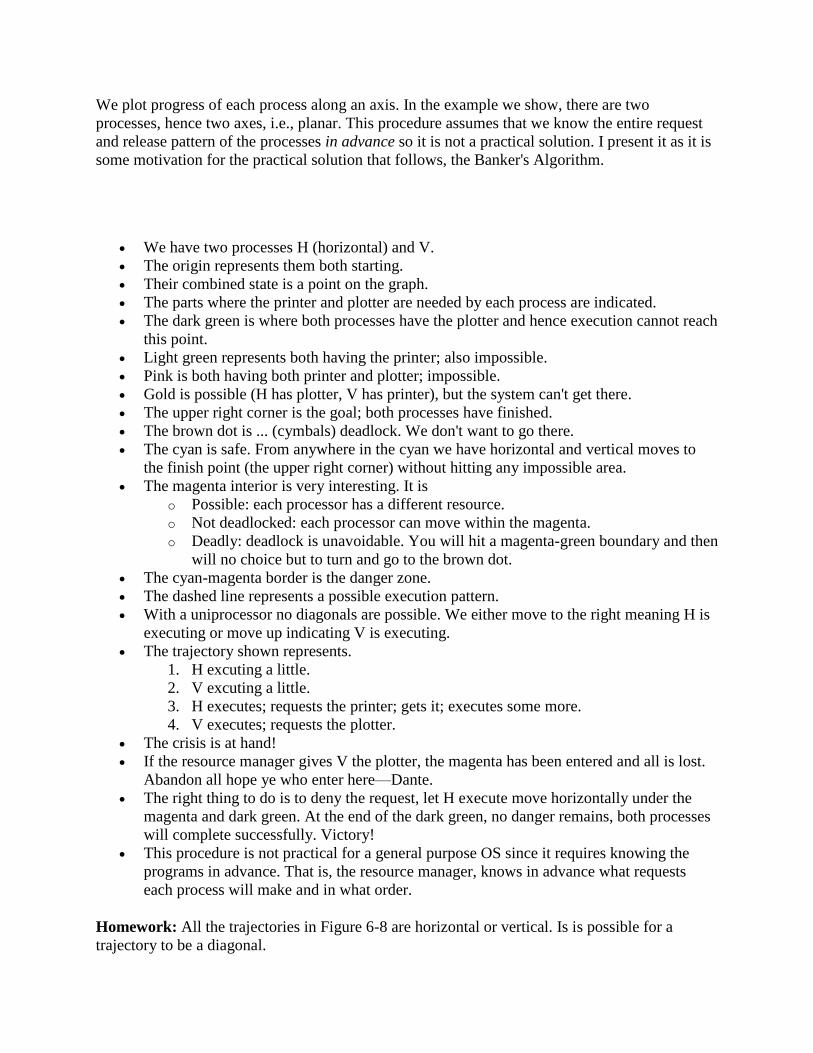
We plot progress of each process along an axis. In the example we show, there are two
processes, hence two axes, i.e., planar. This procedure assumes that we know the entire request
and release pattern of the processes in advance so it is not a practical solution. I present it as it is
some motivation for the practical solution that follows, the Banker's Algorithm.
We have two processes H (horizontal) and V.
The origin represents them both starting.
Their combined state is a point on the graph.
The parts where the printer and plotter are needed by each process are indicated.
The dark green is where both processes have the plotter and hence execution cannot reach
this point.
Light green represents both having the printer; also impossible.
Pink is both having both printer and plotter; impossible.
Gold is possible (H has plotter, V has printer), but the system can't get there.
The upper right corner is the goal; both processes have finished.
The brown dot is ... (cymbals) deadlock. We don't want to go there.
The cyan is safe. From anywhere in the cyan we have horizontal and vertical moves to
the finish point (the upper right corner) without hitting any impossible area.
The magenta interior is very interesting. It is
o Possible: each processor has a different resource.
o Not deadlocked: each processor can move within the magenta.
o Deadly: deadlock is unavoidable. You will hit a magenta-green boundary and then
will no choice but to turn and go to the brown dot.
The cyan-magenta border is the danger zone.
The dashed line represents a possible execution pattern.
With a uniprocessor no diagonals are possible. We either move to the right meaning H is
executing or move up indicating V is executing.
The trajectory shown represents.
1. H excuting a little.
2. V excuting a little.
3. H executes; requests the printer; gets it; executes some more.
4. V executes; requests the plotter.
The crisis is at hand!
If the resource manager gives V the plotter, the magenta has been entered and all is lost.
Abandon all hope ye who enter here—Dante.
The right thing to do is to deny the request, let H execute move horizontally under the
magenta and dark green. At the end of the dark green, no danger remains, both processes
will complete successfully. Victory!
This procedure is not practical for a general purpose OS since it requires knowing the
programs in advance. That is, the resource manager, knows in advance what requests
each process will make and in what order.
Homework: All the trajectories in Figure 6-8 are horizontal or vertical. Is is possible for a
trajectory to be a diagonal.
Homework: 11, 12.
6.5.2 Safe States
Avoiding deadlocks given some extra knowledge.
Not surprisingly, the resource manager knows how many units of each resource it had to
begin with.
Also it knows how many units of each resource it has given to each process.
It would be great to see all the programs in advance and thus know all future requests, but
that is asking for too much.
Instead, when each process starts, it announces its maximum usage. That is each process,
before making any resource requests, tells the resource manager the maximum number of
units of each resource the process can possible need. This is called the claim of the
process.
o If the claim is greater than the total number of units in the system the resource
manager kills the process when receiving the claim (or returns an error code so
that the process can make a new claim).
o If during the run the process asks for more than its claim, the process is aborted
(or an error code is returned and no resources are allocated).
o If a process claims more than it needs, the result is that the resource manager will
be more conservative than need be and there will be more waiting.
Definition: A state is safe if there is an ordering of the processes such that: if the processes are
run in this order, they will all terminate (assuming none exceeds its claim and assuming each
would terminate if all its requests are granted).
Recall the comparison made above between detecting deadlocks (with multi-unit resources) and
the banker's algorithm (which stays in safe states).
The deadlock detection algorithm given makes the most optimistic assumption about a
running process: it will return all its resources and terminate normally. If we still find
processes that remain blocked, they are deadlocked.
The banker's algorithm makes the most pessimistic assumption about a running process:
it immediately asks for all the resources it can (i.e., up to its initial claim). If, even with
such demanding processes, the resource manager can assure that all process terminates,
then we can ensure that deadlock is avoided.
In the definition of a safe state no assumption is made about the running processes. That is, for a
state to be safe, termination must occur no matter what the processes do (providing each would
terminate if run alone and each never exceeds its claims). Making no assumption on a process's
behavior is the same as making the most pessimistic assumption.
Remark: When I say pessimistic I am speaking from the point of view of the resource manager.
From the manager's viewpoint, the worst thing a process can do is request resources.
Give an example of each of the following four possibilities. A state that is
1. Safe and deadlocked—not possible.
2. Safe and not deadlocked—a trivial is example is a graph with no arcs.
3. Not safe and deadlocked—easy (any deadlocked state).
4. Not safe and not deadlocked—interesting.
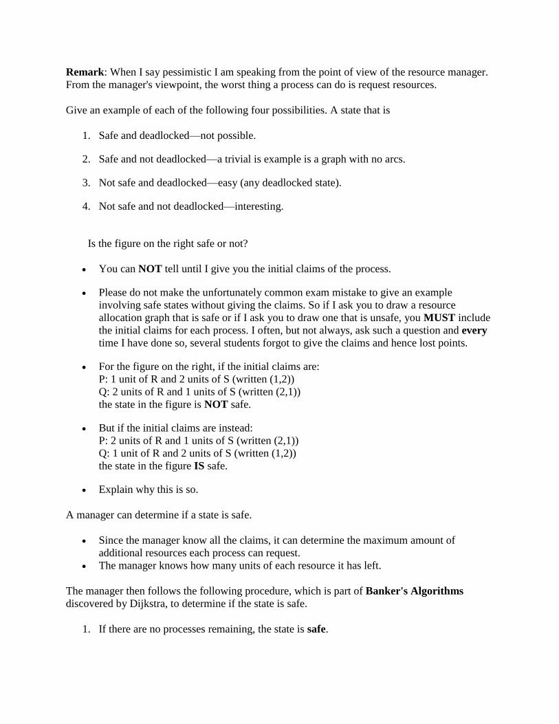
Is the figure on the right safe or not?
You can NOT tell until I give you the initial claims of the process.
Please do not make the unfortunately common exam mistake to give an example
involving safe states without giving the claims. So if I ask you to draw a resource
allocation graph that is safe or if I ask you to draw one that is unsafe, you MUST include
the initial claims for each process. I often, but not always, ask such a question and every
time I have done so, several students forgot to give the claims and hence lost points.
For the figure on the right, if the initial claims are:
P: 1 unit of R and 2 units of S (written (1,2))
Q: 2 units of R and 1 units of S (written (2,1))
the state in the figure is NOT safe.
But if the initial claims are instead:
P: 2 units of R and 1 units of S (written (2,1))
Q: 1 unit of R and 2 units of S (written (1,2))
the state in the figure IS safe.
Explain why this is so.
A manager can determine if a state is safe.
Since the manager know all the claims, it can determine the maximum amount of
additional resources each process can request.
The manager knows how many units of each resource it has left.
The manager then follows the following procedure, which is part of Banker's Algorithms
discovered by Dijkstra, to determine if the state is safe.
1. If there are no processes remaining, the state is safe.
2. Seek a process P whose maximum additional request for each resource type is less than
what remains for that resource type.
o If no such process can be found, then the state is not safe.
o If such a P can be found, the banker (manager) knows that if it refuses all requests
except those from P, then it will be able to satisfy all of P's requests. Why?
Ans: Look at how P was chosen.
3. The banker now pretends that P has terminated (since the banker knows that it can
guarantee this will happen). Hence the banker pretends that all of P's currently held
resources are returned. This makes the banker richer and hence perhaps a process that
was not eligible to be chosen as P previously, can now be chosen.
4. Repeat these steps.
Example 1
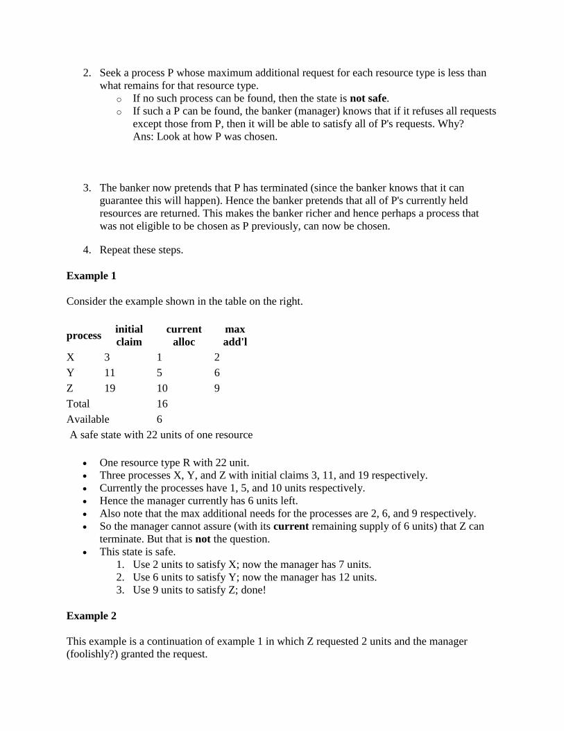
Consider the example shown in the table on the right.
process initial
claim
current
alloc
max
add'l
X 3 1 2
Y 11 5 6
Z 19 10 9
Total 16
Available 6
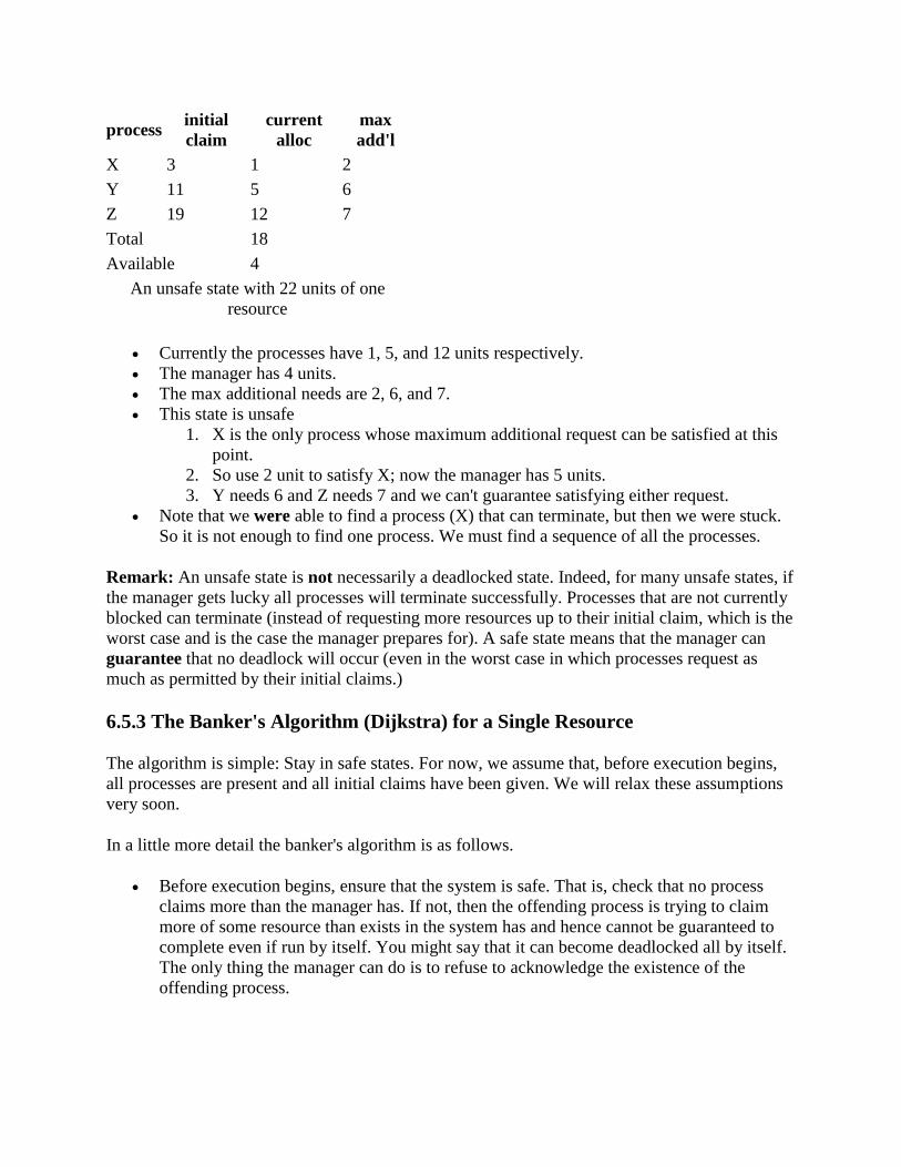
A safe state with 22 units of one resource
One resource type R with 22 unit.
Three processes X, Y, and Z with initial claims 3, 11, and 19 respectively.
Currently the processes have 1, 5, and 10 units respectively.
Hence the manager currently has 6 units left.
Also note that the max additional needs for the processes are 2, 6, and 9 respectively.
So the manager cannot assure (with its current remaining supply of 6 units) that Z can
terminate. But that is not the question.
This state is safe.
1. Use 2 units to satisfy X; now the manager has 7 units.
2. Use 6 units to satisfy Y; now the manager has 12 units.
3. Use 9 units to satisfy Z; done!
Example 2
This example is a continuation of example 1 in which Z requested 2 units and the manager
(foolishly?) granted the request.
process initial
claim
current
alloc
max
add'l
X 3 1 2
Y 11 5 6
Z 19 12 7
Total 18
Available 4
An unsafe state with 22 units of one
resource
Currently the processes have 1, 5, and 12 units respectively.
The manager has 4 units.
The max additional needs are 2, 6, and 7.
This state is unsafe
1. X is the only process whose maximum additional request can be satisfied at this
point.
2. So use 2 unit to satisfy X; now the manager has 5 units.
3. Y needs 6 and Z needs 7 and we can't guarantee satisfying either request.
Note that we were able to find a process (X) that can terminate, but then we were stuck.
So it is not enough to find one process. We must find a sequence of all the processes.
Remark: An unsafe state is not necessarily a deadlocked state. Indeed, for many unsafe states, if
the manager gets lucky all processes will terminate successfully. Processes that are not currently
blocked can terminate (instead of requesting more resources up to their initial claim, which is the
worst case and is the case the manager prepares for). A safe state means that the manager can
guarantee that no deadlock will occur (even in the worst case in which processes request as
much as permitted by their initial claims.)
6.5.3 The Banker's Algorithm (Dijkstra) for a Single Resource
The algorithm is simple: Stay in safe states. For now, we assume that, before execution begins,
all processes are present and all initial claims have been given. We will relax these assumptions
very soon.
In a little more detail the banker's algorithm is as follows.
Before execution begins, ensure that the system is safe. That is, check that no process
claims more than the manager has. If not, then the offending process is trying to claim
more of some resource than exists in the system has and hence cannot be guaranteed to
complete even if run by itself. You might say that it can become deadlocked all by itself.
The only thing the manager can do is to refuse to acknowledge the existence of the
offending process.
When the manager receives a request, it pretends to grant it, and then checks if the
resulting state is safe. If it is safe, the request is really granted; if it is not safe the process
is blocked (that is, the request is held up).
When a resource is returned, the manager (politely thanks the process and then) checks to
see if the first pending requests can be granted (i.e., if the result would now be safe). If so
the pending request is granted. Whether or not the request was granted, the manager
checks to see if the next pending request can be granted, etc.
Homework: 16.
6.5.4 The Banker's Algorithm for Multiple Resources
At a high level the algorithm is identical to the one for a single resource type: Stay in safe states.
But what is a safe state in this new setting?
The same definition (if processes are run in a certain order they will all terminate).
Checking for safety is the same idea as above. The difference is that to tell if there are enough
free resources for a processes to terminate, the manager must check that for all resource types,
the number of free units is at least equal to the max additional need of the process.
Homework: Consider a system containing a total of 12 units of resource R and 24 units of
resource S managed by the banker's algorithm. There are three processes P1, P2, and P3. P1's
claim is 0 units of R and 12 units of S, written (0,12). P2's claim is (8,15). P3's claim is (8,20).
Currently P1 has 4 units of S, P2 has 8 units of R, P3 has 8 units of S, and there are no
outstanding requests.
1. What is the largest number of units of S that P1 can request at this point that the banker
will grant?
2. If P2 instead of P1 makes the request, what is the largest number of units of S that the
banker will grant?
3. If P3 instead of P1 or P2 makes the request, what is the largest number of units of S that
the banker will grant?
Remark: Remind me to go over this one next time.
Limitations of the Banker's Algorithm
Often users don't know the maximum requests a process will make. They can estimate
conservatively (i.e., use big numbers for the claim) but then the manager becomes very
conservative.
New processes arriving cause a problem (but not so bad as Tanenbaum suggests).
o The process's claim must be less than the total number of units of the resource in
the system. If not, the process is not accepted by the manager.
o Since the state without the new process is safe, so is the state with the new
process! Just use the process order the banker had originally and put the new
process at the end.
o Insuring fairness (starvation freedom) needs a little more work, but isn't too hard
either (once an hour stop taking new processes until all current processes finish).
A resource can become unavailable (e.g., a CD-ROM drive might break). This can result
in an unsafe state and deadlock.
Homework: 22, 25, and 30. There is an interesting typo in 22. A has claimed 3 units of resource
5, but there are only 2 units in the entire system. Change the problem by having B both claim and
be allocated 1 unit of resource 5.
6.7 Other Issues
6.7.1 Two-phase locking
This is covered (MUCH better) in a database text. We will skip it.
6.7.2 Communication Deadlocks
We have mostly considered actually hardware resources such as printers, but have also
considered more abstract resources such as semaphores.
There are other possibilities. For example a server often waits for a client to make a request. But
if the request msg is lost the server is still waiting for the client and the client is waiting for the
server to respond to the (lost) last request. Each will wait for the other forever, a deadlock.
A solution to this communication deadlock would be to use a timeout so that the client
eventually determines that the msg was lost and sends another.
But it is not nearly that simple: The msg might have been greatly delayed and now the server will
get two requests, which could be bad, and is likely to send two replies, which also might be bad.
This gives rise to the serious subject of communication protocols.
6.7.3 Livelock
Instead of blocking when a resource is not available, a process may (wait and then) try again to
obtain it. Now assume process A has the printer, and B the CD-ROM, and each process wants
the other resource as well. A will repeatedly request the CD-ROM and B will repeatedly request
the printer. Neither can ever succeed since the other process holds the desired resource. Since no
process is blocked, this is not technically deadlock, but a related concept called livelock.
6.7.4 Starvation
As usual FCFS is a good cure. Often this is done by priority aging and picking the highest
priority process to get the resource. Also can periodically stop accepting new processes until all
old ones get their resources.
6.8 Research on Deadlocks
6.9 Summary
Read.
Operating Systems
Start Lecture #9
Remark: Lab 3 assigned. It is due in 2 weeks on 10 November 2010.
Chapter 3 Memory Management
Also called storage management or space management.
The memory manager must deal with the storage hierarchy present in modern machines.
The hierarchy consists of registers (the highest level), cache, central memory, disk, tape
(backup).
Various (hardware and software) memory managers moves data from level to level of the
hierarchy.
We are concerned with the central memory ↔ disk boundary.
The same questions are asked about the cache ↔ central memory boundary when one
studies computer architecture. Surprisingly, the terminology is almost completely
different!
When should we move data up to a higher level?
o Fetch on demand (e.g. demand paging, which is dominant now and which we
For example, consider the .html extension in class-notes.html, the name of the file we are
viewing. Depending on the system and application, these extensions can have little or great
significance. The extensions can be
1. Conventions just for humans. For example letter.teq (my convention) signifies to me that
this letter is written using the troff text-formatting language and employs the tbl
preprocessor to handle tables and the eqn preprocessor to handle mathematical equations.
Neither linux, troff, tbl, nor equ place any significance in the .teq extension.
2. Conventions giving default behavior for some programs.
o The emacs editor by default edits .html files in html mode. However, emacs can
edit such files in any mode and can edit any file in html mode. It just needs to be
told to do so during the editing session.
o The firefox browser assumes that an .html extension signifies that the file is
written in the html markup language. However, having <html> ... </html> inside
the file works as well.
o The gzip file compressor/decompressor appends the .gz extension to files it
compresses, but accepts a --suffix flag to specify another extension.
3. Default behaviors for the operating system or window manager or desktop environment.
o Click on .xls file in windows and excel is started.
o Click on .xls file in nautilus under linux and openoffice is started.
4. Required for certain programs.
o The gnu C compiler (and probably other C compilers) requires C programs be
have the .c (or .h) extension, and requires assembler programs to have the .s
extension.
5. Required by the operating system
o MS-DOS treats .com files specially.
Operating Systems
Start Lecture #12
Case Sensitive?
Should file names be case sensitive. For example, do x.y, X.Y, x.Y all name the same file? There
is no clear answer.
Unix-like systems employ case sensitive file names so the three names given above are distinct. Windows systems employ case insensitive file names to the three names given above are
equivalent. Mathematicians (and others) often "consider an element x of a set X" so use case sensitive
naming. Normal English (and other natural language) usage often employs case insensitivity (e.g.
capitalizing a word at the beginning of a sentence does not change the word).
4.1.2 File Structure
How should the file be structured. Alternatively, how does the OS interpret the contents of a file.
A file can be interpreted as a
1. Byte stream o Unix, dos, windows. o Maximum flexibility. o Minimum structure. o All structure on a file is imposed by the applications that use it, not by the system itself.
2. (fixed size-) Record stream: Out of date o 80-character records for card images. o 133-character records for line printer files. Column 1 was for control (e.g., new page)
Remaining 132 characters were printed.
3. Varied and complicated beast. o Indexed sequential. o B-trees. o Supports rapidly finding a record with a specific key. o Supports retrieving (varying size) records in key order.
o Treated in depth in database courses.
4.1.3 File Types
The traditional file is simply a collection of data that forms the unit of sharing for processes,
even concurrent processes. These are called regular files.
The advantages of uniform naming have encouraged the inclusion in the file system of objects
that are not simply collections of data.
Regular Files
Text vs Binary Files
Some regular files contain lines of text and are called (not surprisingly) text files or ascii files.
Each text line concludes with some end of line indication: on unix and recent MacOS this is a
newline (a.k.a line feed), in MS-DOS it is the two character sequence carriage return followed by
newline, and in earlier MacOS it was carriage return.
Ascii, with only 7 bits per character, is poorly suited for most human languages other than
English. Latin-1 (8 bits) is a little better with support for most Western European Languages.
Perhaps, with growing support for more varied character sets, ascii files will be replaced by
unicode (16 bits) files. The Java and Ada programming languages (and perhaps others) already
support unicode.
An advantage of all these formats is that they can be directly printed on a terminal or printer.
Other regular files, often referred to as binary files, do not represent a sequence of characters.
For example, a four-byte, twos-complement representation of integers in the range from roughly
-2 billion to +2 billion is definitely not to be thought of as 4 latin-1 characters, one per byte.
Application Imposed File Structure
Just because a file is unstructured (i.e., is a byte stream) from the OS perspective does not mean
that applications cannot impose structure on the bytes. So a document written without any
explicit formatting in MS word is not simply a sequence of ascii (or latin-1 or unicode)
characters.
On unix, an executable file must begin with one of certain magic numbers in the first few bytes.
For a native executable, the remainder of the file has a well defined format.
Another option is for the magic number to be the ascii representation of the two characters #! in
which case the next several characters specify the location of the executable program that is to be
run with the current file fed in as input. That is how interpreted (as opposed to compiled)
languages work in unix.
#!/usr/bin/perl
perl script
Strongly Typed Files
In some systems the type of the file (which is often specified by the extension) determines what
you can do with the file. This make the easy and (hopefully) common case easier and, more
importantly, safer.
It tends to make the unusual case harder. For example, you have a program that turns out data
(.dat) files. Now you want to use it to turn out a java file, but the type of the output is data and
cannot be easily converted to type java and hence cannot be given to the java compiler.
Other-Than-Regular Files
We will discuss several file types that are not called regular.
1. Directories. 2. Symbolic Links, which are used to give alternate names to files. 3. Special files (for devices). These use the naming power of files to unify many actions. 4. dir # prints on screen
5. dir > file # result put in a file
6. dir > /dev/audio # results sent to speaker (sounds awful)
4.1.4 File Access
There are two possibilities, sequential access and random access (a.k.a. direct access).
With sequential access, each access to a given file starts where the previous access to that file
finished (the first access to the file starts at the beginning of the file). Sequential access is the
most common and gives the highest performance. For some devices (e.g. magnetic or paper tape)
access must be sequential.
With random access, the bytes are accessed in any order. Thus each access must specify which
bytes are desired. This is done either by having each read/write specify the starting location or
by defining another system call (often named seek) that specifies the starting location for the
next read/write.
For example, in unix, if no seek occurs between two read/write operations, then the second
begins where the first finished. That is, unix treats a sequences of reads and writes as
sequential, but supports seeking to achieve random access.
Previously, files were declared to be sequential or random. Modern systems do not do this.
Instead all files are random, and optimizations are applied as the system dynamically determines
that a file is (probably) being accessed sequentially.
Various properties that can be specified for a file For example:
hidden do not dump owner key length (for keyed files)
4.1.6 File Operations
Create. The effect of create is essential if a system is to add files. However, it need not be a separate system call. (For example, it can be merged with open).
Delete. Essential, if a system is to delete files. Open. Not essential. An optimization in which a process translates a file name to the
corresponding disk locations only once per execution rather than once per access. We shall see that for the unix inode-based file systems, this translation can be quite expensive.
Close. Not essential. Frees resources without waiting for the process to terminate. Read. Essential. Must specify filename, file location, number of bytes, and a buffer into which
the data is to be placed. Several of these parameters can be set by other system calls and in many operating systems they are.
Write. Essential, if updates are to be supported. See read for parameters. Seek. Not essential (could be in read/write). Specify the offset of the next (read or write) access
to this file. Get attributes. Essential if attributes are to be used. Set attributes. Essential if attributes are to be user settable. Rename. Tanenbaum has strange words. Copy and delete is not an acceptable substitute for big
files. Moreover, copy-delete is not atomic. Indeed link-delete is not atomic so, even if link (discussed below) is provided, renaming a file adds functionality.
Homework: 4, 5.
4.1.7 An Example Program Using File System Calls
Homework: Read and understand copyfile.
Note the error checks. Specifically, the code checks the return value from each I/O system call. It
is a common error to assume that
1. Open always succeeds. It can fail due to the file not existing or the process having inadequate permissions.
2. Read always succeeds. An end of file can occur. Fewer than expected bytes could have been read. Also the file descriptor could be bad, but this should have been caught when checking the return value from open.
3. Create always succeeds. It can fail when the disk (partition) is full, or when the process has inadequate permissions.
4. Write always succeeds. It too can fail when the disk is full or the process has inadequate permissions.
4.2 Directories
Directories form the primary unit of organization for the filesystem.
4.2.1-4.2.3 Single-Level (Two-Level) and Hierarchical Directory Systems
One often refers to the level structure of a directory system. It is easy to be fooled by the names
given. A single level directory structure results in a file system tree with two levels: the single
root directory and (all) the files in this directory. That is, there is one level of directories and
another level of files so the full file system tree has two levels.
Possibilities.
One directory in the system (single-level). This possibility is illustrated by the top left tree. One directory per user and a root above these (two-level). This possibility is illustrated by the
top right tree. One tree in the system. This possibility is illustrated by the bottom tree. One tree per user with a root above. This possibility is also illustrated by the bottom tree. One forest in the system. This possibility is illustrated by viewing all three trees as together
constituting the file system forest. One forest per user. This possibility is not illustrated. To do so would require, for each user, one
picture similar to the entire picture on the right.
These possibilities are not as wildly different as they sound or as the pictures suggests.
Assume the system has only one directory, but also assume the character / is allowed in a file name. Then one could fake a tree by having a file named /allan/gottlieb/courses/os/class-notes.html rather than a directory allan, a subdirectory gottlieb, ..., a file class-notes.html.
The Dos (windows) file system is a forest, the Unix file system is a tree (until we learn about links below, but even then it is not a forest). In Dos, there is no common parent of a:\ and c:\, so the file system is not a tree. But Windows explorer makes the dos forest look quite a bit like a tree.
You can get an effect similar to one X per user by having just one X in the system and having permissions that permits each user to visit only a subset. Of course if the system doesn't have permissions, this is not possible.
Today's multiuser systems have a tree per system or a forest per system. This is not strictly true due to links, which we will study soon.
Simple embedded systems often use a one-level directory system.
You can specify the location of a file in the file hierarchy by using either an absolute or a
relative path to the file.
An absolute path starts at the (or one of the, if we have a forest) root(s). A relative path starts at the current (a.k.a working) directory. In order to support relative paths,
a process must know its current directory and there is such a field in the process control block. The special directories . and .. represent the current directory and the parent of the current
directory respectively.
Homework: Give 8 different path names for the file /etc/passwd.
Homework: 7.
4.2.5 Directory Operations
1. Create. Produces an empty directory. Normally the directory created actually contains . and .., so is not really empty
2. Delete. The delete system call requires the directory to be empty (i.e., to contain just . and ..). Delete commands intended for users have options that cause the command to first empty the directory (except for . and ..) and then delete it. These user commands make use of both file and directory delete system calls.
3. Opendir. As with the file open system call, opendir creates a handle for the directory that speeds future access by eliminating the need to process the name of the directory.
4. Closedir. As with the file close system call, closedir is an optimization that enables the system to free resources prior to process termination.
5. Readdir. In the old days (of unix) one could read directories as files so there was no special readdir (or opendir/closedir) system call. It was then believed that the uniform treatment would make programming (or at least system understanding) easier as there was less to learn.
However, experience has taught that this was a poor idea since the structure of directories
was exposed to users. Early unix had a simple directory structure and there was only one
type of structure for all implementations. Modern systems have more sophisticated
structures and more importantly they are not fixed across implementations. So if
programs used read() to read directories, the programs would have to be changed
whenever the structure of a directory changed. Now we have a readdir() system call that
knows the structure of directories. Therefore if the structure is changed only readdir()
need be changed.
This is an example of the software principle of information hiding.
6. Rename. Similar to the file rename system call. Again note that rename is atomic; whereas, creating a new directory, moving the contents, and then removing the old one is not.
7. Link. Add another name for a file; discussed below.
8. Unlink. Remove a directory entry. This is how a file is deleted. However, if there are many links and just one is unlinked, the file remains. Unlink is discussed in more detail below.
9. There is no Writedir operation. Directories are written as a side effect of other operations.
4.3 File System Implementation
Now that we understand how the file system looks to a user, we turn our attention to how it is
implemented.
4.3.1 File System Layout
We look at how the file systems are laid out on disk in modern PCs. Much of this is required by
the bios so all PC operating systems have the same lowest level layout. I do not know the
corresponding layout for mainframe systems or supercomputers.
A system often has more than one physical disk (3e forgot this). The first disk is the boot disk.
How do we determine which is the first disk?
1. Easiest case: only one disk. 2. Only one disk controller. The disk with the lowest number is the boot disk. The numbering is
system dependent, for SCSI (small computer system interconnect, now used on big computers as well) you set switches on the drive itself (normally jumpers).
3. Multiple disk controllers. The controllers are ordered in a system dependent way.
The BIOS reads the first sector (smallest addressable unit of a disk) of the boot disk into memory
and transfers control to it. A sector contains 512 bytes. The contents of this particular sector is
called the MBR (master boot record).
The MBR contains two key components: the partition table and the first-level loader.
A disk can be logically divided into variable size partitions, each acting as a logical disk. That is, normally each partition holds a complete file system. The partition table (like a process's page table) gives the starting point of each partition. It is actually more like the segment table of a pure segmentation system since the objects pointed to (partitions and segments) are of variable size. As with segments, the size of each partition is stored in the corresponding entry of the partition table.
One partition in the partition table is marked as the active partition. The first level loader then loads 2nd-level loader, which resides in the first sector of the active
partition, and transfers control to it. This sector is called the boot sector or boot block. The boot block then loads the OS (actually it can load another loader, etc)
The contents vary from one file system to another but there is some commonality.
Each partition has a boot block as mentioned above. Each partition must have some information saying what type of file system is stored in this
partition. The region containing this and other administrative information is often called the superblock. The location of the superblock is fixed.
The location of the root directory is either fixed, or is in the superblock, or (as in unix i-node file systems) the root i-node is in a fixed location. The root i-node points to the root directory. We will have more to say about i-nodes below.
Free (i.e., available) disk blocks must be maintained. If these blocks are linked together, the head of the list (or a pointer to it) must be in a well defined spot. If a bitmap is used, it (or a pointer to it) must be in a well defined place.
Files and directories (i.e., in use disk blocks). These are of course the reason we have the file system.
For i-node based systems, the i-nodes are normally stored in a separate region of the partition.
4.3.2 Implementing Files
A fundamental property of disks is that they cannot read or write single bytes. The smallest unit
that can be read or written is called a sector and is normally 512 bytes (plus error
correction/detection bytes). This is a property of the hardware, not the operating system.
The operating system reads or writes disk blocks. The size of a block is a multiple (normally a
power of 2) of the size of a sector. Since sectors are usually (always?) 512 bytes, the block size
can be 512, 1024=1K, 2K, 4K, 8K, 16K, etc. The most common block sizes today are 4K and
8K.
So files will be composed of blocks.
When we studied memory management, we had to worry about fragmentation, processes
growing and shrinking, compaction, etc.. Many of these same considerations apply to files; the
difference is that instead of a memory region being composed of bytes, a file is composed of
blocks.
Contiguous Allocation
Recall the simplest form of memory management beyond uniprogramming was OS/MFT where
memory was divided into a very few regions and each process was given one of these regions.
The analogue for disks would be to give each file an entire partition. This is too inflexible and is
not used for files.
The next simplest memory management scheme was the one used in OS/MVT, where the
memory for a process was contiguous.
The analogous scheme for files is called contiguous allocation. Each entire file is stored as one piece.
This scheme is simple and fast for access since, as we shall see next chapter, disks give much better performance when accessed sequentially.
However contiguous allocation is problematic for growing files. o If a growing file reaches another file, the system must move files. o The extreme would be to compactify the disk, which entails moving many files and the
resulting configuration with no holes will have trouble with any file growing (except the last file).
o OS/MVT had the analogous problem when jobs grew. As with memory, there is the problem of external fragmentation. Contiguous allocation is no longer used for general purpose rewritable file systems. It is ideal for file systems where files do not change size. It is used for CD-ROM file systems. It is used (almost) for DVD file systems. A DVD movie is a few gigabytes in size but the 30 bit file
length field limits files to 1 gigabyte so each movie is composed of a few contiguous files. The reason I said almost is that the terminology used is that the movie is one file stored as a sequence of extents and only the extents are contiguous.
Homework: 10. There is a typo: the first sentence should end at the first comma. Contiguous
allocation of files leads to disk fragmentation.
Linked Allocation
A file is an ordered sequence of blocks. We just considered storing the blocks one right after the
other (contiguous) the same way that one can store an in-memory list as an array. The other
common method for in-memory lists is to link the elements together via pointers. This can also
be done for files as follows.
The directory entry for the file contains a pointer to the first block of the file. Each file block contains a pointer to the next.
However
This scheme gives horrible performance for random access: N disk accesses are needed to access block N.
Having the pointer inside the block is a nuisance.
As a result this implementation of linked allocation is not used.
Consider the following two code segments that store the same data but in a different order. The
first is analogous to the horrible linked list file organization above and the second is analogous to
the ms-dos FAT file system we study next.
struct node_type {
float data; float node_data[100];
int next; int node_next[100];
} node[100]
With the second arrangement the data can be stored far away from the next pointers. In FAT this
idea is taken to an extreme: The data, which is large (a disk block), is stored on disk; whereas,
the next pointers, which are small (each is an integer) are stored in memory in a File Allocation
Table or FAT. (When the system is shut down the FAT is copied to disk and when the system is
booted, the FAT is copied to memory.)
The FAT (File Allocation Table) File System
The FAT file system stores each file as a linked list of disk blocks. The blocks, which contain
file data only (not the linked list structure) are stored on disk. The pointers implementing the
linked list are stored in memory.
There is a long lineage of FAT file systems (FAT-12, FAT-16, vfat, ...) all of which use the file allocation table. The following description of FAT is fairly generic and applies to all of them.
FAT was the file system used by dos and and early versions of Windows. The NT series of Windows (NT, 2000, XP, Vista) supports FAT as well as the superior NTFS (NT
File System). Linux has full support for FAT (and improving support for NTFS). FAT is used on flash RAMS (USB memory sticks) as well as memory cards for digital cameras. The directory entry for a file points to first block (i.e., the directory entry specifies the block
number). A FAT is maintained in memory having one (1-word) entry for each disk block. The entry for
block N contains the block number of the next block in the same file as N. If block N is the last block of a file, the entry is EOF.
This implements linked allocation but the links are stored separate from the data. The time needed to access a random block is still is linear in the size of the file but now all the
references are to the FAT, which is in memory. So it is bad for random accesses, but not nearly as horrible as plain linked allocation.
The size of the table is one pointer per disk block. So the ratio of the disk space supported to the memory space needed is
(size of a disk block) / (size of a pointer)
If the block size is 8KB and a pointer is 2B, the memory requirement is 1/4 megabyte for each
disk gigabyte. Large but not prohibitive. (While 8KB is reasonable today for blocksize, 2B
pointers is not since that would mean the largest partition could be 216 blocks = 216×213 bytes =
229 bytes = 1/2 GB, which is much too small.)
If the block size is 512B (the sector size of most disks) and a pointer is 8B then the memory requirement is 16 megabytes for each disk gigabyte, which would most likely be prohibitive.
The Unix Inode-based Filesystem
Continuing the idea of adapting storage schemes from other regimes to file storage, why don't we
mimic the idea of (non-demand) paging and have a table giving, for each block of the file, where
on the disk that file block is stored? In other words a ``file block table'' mapping each file block
to its corresponding disk block. This is the idea of (the first part of) the unix i-node solution,
which we study next.
Although Linux and other Unix and Unix-like operating systems have a variety of file systems,
the most widely used Unix file systems are i-node based as was the original Unix file system
from Bell Labs.
There is some question of what the i stands for. The consensus seems to be index. Now,
however, people often write inode (not i-node) and don't view the i as standing for anything.
Inode based systems have the following properties.
1. Each file and directory has an associated inode, which enables the system to find the blocks of the file or directory.
2. The inode associated with the root (called the root inode) is at a known location on the disk. In particular, the root inode can be found by the system.
3. The directory entry for a file contains a pointer to the file's i-node.
4. The directory entry for a subdirectory contains a pointer to the subdirectory's i-node.
5. The metadata for a file or directory is stored in the corresponding inode.
6. The inode itself points to the first few data blocks, often called direct blocks. (As of June 2006, the main Linux file system organization used twelve direct blocks.) In the diagram on the right, the inode contains pointers to six direct blocks and all data blocks are colored blue.
7. The inode also points to an indirect block, which then points to a number of disk blocks. The number is K=(blocksize)/(pointersize). In the diagram, the indirect blocks (also called single indirect blocks) are colored green.
8. The inode also points to a double indirect block, which points to a K single indirect blocks. each of which points to N data blocks. In the diagram, double indirect blocks are colored magenta.
9. For some implementations there is a triple indirect block as well. A triple indirect block points to K double indirect blocks, which point ... . In the diagram, the triple indirect block is colored yellow.
10. The i-node is in memory for open files. So references to direct blocks require just one I/O.
11. For big files most references require two I/Os (indirect + data).
12. For huge files most references require three I/Os (double indirect, indirect, and data).
13. For humongous files most references require four I/Os.
14. Actually, fewer I/Os are normally required due to caching.
Retrieving a Block in an Inode-Based File System
Given a block number (byte number / block size), how do you find the block?
Specifically assume
1. The file system does not have a triple indirect block. 2. We desire block number N, where N=0 is the first block. 3. There are D direct pointers in the inode. These pointers are numbered 0..(D-1). 4. There are K pointers in each indirect block. These pointers are numbered 0..(K-1).
If N < D // This is a direct block in the i-node
use direct pointer N in the i-node
else if N < D + K // The single indirect block has a pointer to this
block
use pointer D in the inode to get the indirect block
the use pointer N-D in the indirect block to get block N
else // This is one of the K*K blocks obtained via the double indirect
block
use pointer D+1 in the inode to get the double indirect block
let P = (N-(D+K)) DIV K // Which single indirect block to use
use pointer P to get the indirect block B
let Q = (N-(D+K)) MOD K // Which pointer in B to use
use pointer Q in B to get block N
For example, let D=12, assume all blocks are 1000B, assume all pointers are 4B. Retrieve the
block containing byte 1,000,000.
K = 1000/4 = 250. Byte 1,000,000 is in block number N=1000. N > D + K so we need the double indirect block. Follow pointer number D+1=13 in the inode to retrieve the double indirect block. P=(1000-262) DIV 250 = 738 DIV 250 = 2. Follow pointer number P=2 in the double indirect block to retrieve the needed single indirect
block. Q=(1000-262) MOD 250 = 738 MOD 250 = 238. Follow pointer number 238 in the single indirect block to retrieve the desired block (block
number 1000).
With a triple indirect block, the ideas are the same, but there is more work.
Homework: Consider an inode-based system with the same parameters as just above, D=12,
1. What is the largest file that can be stored. 2. How much space is used to store this largest possible file (assume the attributes require 64B)? 3. What percentage of the space used actually holds file data? 4. Repeat all the above, now assuming the file system supports a triple indirect block.
End of Problem
Operating Systems
Start Lecture #13
4.3.3 Implementing Directories
Recall that the primary function of a directory is to map the file name (in ASCII, Unicode, or
some other text-based encoding) to whatever is needed to retrieve the data of the file itself.
There are several ways to do this depending on how files are stored.
For sequentially allocated files, the directory entry for a file contains the starting address on the disk and the file size. Since disks can only be accessed by sectors, we store the sector number. The system can choose to start all files on a block (rather than sector) boundary in which case the block number, which is smaller, is stored instead.
For linked allocation (pure linked or FAT-based) the directory entry again points to the first block of the file.
For inode-based file systems, the directory entry points to the inode.
Another important function is to enable the retrieval of the various attributes (e.g., length, owner,
size, permissions, etc.) associated with a given file.
One possibility is to store the attributes in the directory entry for the file. Windows does this. Another possibility for inode-based systems, is to store the attributes in the inode as we have
suggested above. The inode-based file systems for Unix-like operating systems do this.
Homework: 25
Long File Names
It is convenient to view the directory as an array of entries, one per file. This view tacitly
assumes that all entries are the same size and, in early operating systems, they were. Most of the
contents of a directory are inherently of a fixed size. The primary exception is the file name.
Early systems placed a severe limit on the maximum length of a file name and allocated this
much space for all names. DOS used an 8+3 naming scheme (8 characters before the dot and 3
after). Unix version 7 limited names to 14 characters.
Later systems raised the limit considerably (255, 1023, etc) and thus allocating the maximum
amount for each entry was inefficient and other schemes were used. Since we are storing variable
size quantities, a number of the consideration that we saw for non-paged memory management
arise here as well.
Searching Directories for a File
The simple scheme is to search the list of directory entries linearly, when looking for an entry
with a specific file name. This scheme becomes inefficient for very large directories containing
hundreds or thousands of files. In this situation a more sophisticated technique (such as hashing
or B-trees) is used.
4.3.4 Shared (Multinamed) Files (Links)
We often think of the files and directories in a file system as forming a tree (or forest). However
in most modern systems this is not necessarily the case, the same file can appear in two different
directories (not two copies of the file, but the same file). It can also appear multiple times in the
same directory, having different names each time.
I like to say that the same file has two different names. One can also think of the file as being
shared by the two directories (but those words don't work so well for a file with two names in the
same directory).
Shared files is Tanenbaum's terminology. If a file exists, one can create another name for it (quite possibly in another directory). This is often called creating another link to the file. Unix has two flavor of links, hard links and symbolic links (a.k.a. symlinks). Dos/windows has shortcuts, which behave somewhat like symlinks, but I don't believe it has an
analogue of hard links. We will concentrate on both flavors of unix links. These links often cause confusion, but I really believe that the diagrams I created make it all
clear.
Hard Links
With unix hard links there are multiple names for the same file and each name has equal status.
The directory entries for both names point to the same inode.
Hard links are thus symmetric multinamed files. When a hard link is created another name is created for the same file. The number of files in the
system is the same before and after the hard link is created. It is not, I repeat NOT, true that one name is the real name and the other one is just a link. Indeed after the hard link has been created it is not possible to tell which was the original name
and which is the newly created link.
For example, the diagram on the right illustrates the result that occurs when, starting with an
empty file system (i.e., just the root directory) one executes
cd /
mkdir /A; mkdir /B
touch /A/X; touch /B/Y
The diagrams in this section use the following conventions
Yellow circles represent ordinary files. Blue squares represent directories. Names are written on the edges. For example, one name for the left circle is /A/X.
o It is not customary to write the names on the edges, normally they are written in the circles and squares.
o When there are no multi-named files, it doesn't matter if they are written in the node or on the edge.
o We will see that when files can have multiple names it is much better to write the name on the edge.
Now we execute
ln /B/Y /A/New
which leads to the next diagram on the right.
Note that there are still exactly 5 inodes and 5 files: two regular files and three directories. All
that has changed is that there is another name for one of the regular files. At this point there are
two equally valid name for the right hand yellow file, /B/Y and /A/New. The fact that /B/Y was
created first is NOT detectable.
The directory entries for both file names point to the same i-node. The file has only one owner (the one who created the file initially). The file has one date of last access (the last access by any of its names), one set of permissions,
one ... . Note the usage: the file nameS (plural) vs the file (singular).
Assume Bob created /B and /B/Y and Alice created /A, /A/X, and /A/New. Later Bob tires of
/B/Y and removes it by executing
rm /B/Y
The file /A/New is still fine (see the diagram on the right). But it is owned by Bob, who can't
find it! If the system enforces quotas Bob will likely be charged (as the owner), but he can
neither find nor delete the file (since Bob cannot unlink, i.e. remove, files from /A).
If, prior to removing /B/Y, Bob had examined its link count (an attribute of the file), he would
have noticed that there is another (hard) link to the file, but would not have been able to
determine in which directory (/A in this case) the hard link was located or what is the name of
the file in that directory (New in this case).
Since hard links are only permitted to files (not directories) the resulting file system is a dag
(directed acyclic graph). That is, there are no directed cycles. We will now proceed to give away
this useful property by studying symlinks, which can point to directories.
Symlinks
As just noted, hard links do NOT create a new file, just another name for an existing file. Once
the hard link is created the two names have equal status.
Symlinks, on the other hand DO create another file, a non-regular file, that itself serves as
another name for the original file. Specifically
Creation of a symlink results in an asymmetric multi-named file. Assuming the original was a regular file, the symlink does indeed have a different status.
When a symlink is created another file is created. The contents of the new file is the name of the original file.
A hard link in contrast is (another name for) the original file. The examples will make this clear.
Again start with an empty file system and this time execute the following code sequence (the
only difference from the above is the addition of a -s).
cd /
mkdir /A; mkdir /B
touch /A/X; touch /B/Y
ln -s /B/Y /A/New
We now have an additional file /A/New, which is a symlink to /B/Y.
The file named /A/New has the name /B/Y as its data (not metadata). The system notices that /A/New is a red diamond (symlink) so reading /A/New will return the
contents of /B/Y (assuming the reader has read permission for /B/Y). It is also possible to read the contents of /A/New itself (those contents are the string /B/Y).
The size of A/New is 4 bytes, one for each character of its contents. If /B/Y is removed, /A/New becomes invalid. If a new /B/Y is created, /A/New is once again valid. Removing /A/New has no effect of /B/Y. Examining /B/Y does not reveal the existence of /A/New. If a user has write permission for /B/Y, then writing /A/New is possible and writes /B/Y.
The bottom line is that, with a hard link, a new name is created for the file. This new name has
equal status with the original name. This can cause some surprises (e.g., you create a link but I
own the file). With a symbolic link a new file is created (owned by the creator naturally) that
contains the name of the original file. We often say the new file points to the original file.
Question: Consider the hard link setup above. If Bob removes /B/Y and then creates another
/B/Y, what happens to /A/New?
Answer: Nothing. /A/New is still a file owned by Bob having the same contents, creation time,
etc. as the original /B/Y.
Question: What about with a symlink?
Answer: /A/New becomes invalid and then valid again, this time pointing to the new /B/Y. (It
can't point to the old /B/Y as that is completely gone.)
Note: Shortcuts in windows contain more than symlinks contain in unix. In addition to the file name of
the original file, they can contain arguments to pass to the file if it is executable. So a shortcut to
Moreover, as was pointed out by students in my 2006-07 fall class, the shortcuts are not a feature
of the windows FAT file system itself, but simply the actions of the command interpreter when
encountering a file named *.lnk
End of Note.
Symlinking a Directory
What happens if the target of the symlink is an existing directory? For example, consider the
code below, which gives rise to the diagram on the right.
cd /
mkdir /A; mkdir /B
touch /A/X; touch /B/Y
ln -s /B /A/New
1. Is there a file named /A/New/Y ? Answer: Yes.
2. What happens if you execute cd /A/New; dir ? Answer: You see a listing of the files in /B, in this case the single file Y.
3. What happens if you execute cd /A/New/.. ? Answer: Not clear! Clearly you are changing directory to the parent directory of /A/New. But is that /A or /? The command interpreter I use offers both possibilities.
o cd -L /A/New/.. takes you to A (L for logical). o cd -P /A/New/.. takes you to / (P for physical). o cd /A/New/.. takes you to A (logical is the default).
4. What did I mean when I said the pictures made it all clear? Answer: From the file system perspective it is clear. It is not always so clear what programs will do.
4.3.5 Log-Structured File Systems
This research project of the early 1990s was inspired by the key observation that systems are
becoming limited in speed by small writes. The factors contributing to this phenomenon were
(and still are).
1. The CPU speed increases have far surpassed the disk speed increases so the system has become I/O limited.
2. The large buffer cache found on modern systems has led to fewer read requests actually requiring I/Os.
3. A disk I/O requires almost 10ms of preparation before any data is transferred, and then can transfer a block in less than 1ms. Thus, a one block transfer spends most of its time getting ready to transfer.
The goal of the log-structured file system project was to design a file system in which all writes
are large and sequential (most of the preparation is eliminated when writes are sequential). These
writes can be thought of as being appended to a log, which gave the project its name.
The project worked with a unix-like file system, i.e. it was i-node based. The system accumulates writes in a buffer until have (say) 1MB to write. When the buffer is full, write it to the end of the disk (treating the disk as a log). Thus writes are sequential and large and hence fast. When any part of a file is changed, the i-node is rewritten. The 1MB units on the disk are called (unfortunately) segments. I will refer to the buffer as the
segment buffer. A segment can contain i-nodes, direct blocks, indirect blocks, blocks forming part of a file, and
blocks forming part of a directory. In short a segment contains the most recently modified (or created) 1MB of blocks.
Note that the now useless overwritten blocks are not reclaimed!
The system keeps a map of where the most recent version of each i-node is located. This map is on disk (but the heavily accessed parts will be in the buffer cache).
So the (most up to date) i-node of a file can be found and from that the entire file can be found. But the disk will fill with garbage since modified blocks are not reclaimed. A cleaner process runs in the background and examines segments starting from the beginning. It
removes overwritten blocks and then adds the remaining blocks to the segment buffer. (This is very much not trivial.)
Thus the disk is compacted and is treated like a circular array of segments.
Despite the advantages given, log-structured file systems have not caught on. They are
incompatible with existing file systems and the cleaner has proved to be difficult.
4.3.6 Journaling File Systems
Many seemingly simple I/O operations are actually composed of sub-actions. For example,
deleting a file on an i-node based system (really this means deleting the last link to the i-node)
requires removing the entry from the directory, placing the i-node on the free list, and placing the
file blocks on the free list.
What happens if the system crashes during a delete and some, but not all three, of the above
actions occur?
If the operations are guaranteed to be done in the order given, then the worst that can occur is that the entry is removed from the directory, but some file blocks and possibly the i-node are not reclaimed. This wastes resources, but is not a disaster.
As we will learn later, I/O performance is sometimes improved if operations are executed out of order.
In that case we can have a directory entry pointing to an i-node that has been freed or an i-node referring to blocks that have been freed.
Since free blocks and i-nodes are later reassigned to other files, the results can be catastrophic.
A journaling file system prevents these problems by using an idea from database theory, namely
transaction logs. To ensure that the multiple sub-actions are all performed, the larger I/O
operation (delete in the example) is broken into 3 steps.
1. Write a log stating what has to be done and ensure it is written to disk. 2. Start doing the sub-actions. 3. When all sub-actions complete, mark the log entry as complete (and eventually erase it)..
After a crash, the log (called a journal) is examined and if there are pending sub-actions, they are
done before the system is made available to users.
Since sub-actions may be repeated (once before the crash, and once after), it is required that they
all be idempotent (applying the action twice is the same as applying it once).
Some history.
IBM's AIX had a journaling file system in 1990. NTFS had journaling from day 1 (1993). Many Unix systems have it now. The main linux file system (ext2) added journaling (and became ext3) in 2001. Journaling
appeared earlier that year in other Linux file systems. Journaling was added to HFS+, the MacOS file system, in 2002. FAT has never had journaling.
4.3.7 Virtual File Systems
A single operating system needs to support a variety of file systems. The software support for
each file system would have to handle the various I/O system calls defined.
Not surprisingly the various file systems often have a great deal in common and large parts of the
implementations would be essentially the same. Thus for software engineering reasons one
would like to abstract out the common part.
This was done by Sun Microsystems when they introduced NFS the Network File System for
Unix and by now most unix-like operating systems have adopted this idea. The common code is
called the VFS layer and is illustrated on the right.
The original motivation for Sun was to support NFS (Network File System), which permits a file
system residing on machine A to be mounted onto a file system residing on machine B. The
result is that by cd'ing to the appropriate directory on machine B, a user with sufficient privileges
can read/write/execute the files in the machine A file system.
Note that mounting one file system onto another (whether they are on different machines or not)
does not require that the two file systems be the same type. For example, I routinely mount FAT
file systems (from MP3 players, cameras, ets) on to my Linux inode file system. The
involvement of multiple file system software components for a single operation is another point
in VFS's favor.
Nonetheless, I consider the idea of VFS to be mainly good (perhaps superb) software
engineering more than OS design. The details are naturally OS specific.
4.4 File System Management and Optimization
Since I/O operations can dominate the time required for complete user processes, considerable
effort has been expended to improve the performance of these operations.
4.4.1 Disk Space Management
All general purpose file systems use a (non-demand) paging algorithm for file storage (read-only
systems, which often use contiguous allocation, are the major exception). Files are broken into
fixed size pieces, called blocks that can be scattered over the disk. Note that although this is
paging, it is not called paging (and may not have an explicit page table).
Actually, it is more complicated since various optimizations are performed to try to have
consecutive blocks of a single file stored consecutively on the disk. This is discussed below.
Note that all the blocks of the file are stored on the disk, i.e., it is not demand paging.
One can imagine systems that do utilize demand-paging-like algorithms for disk block storage.
In such a system only some of the file blocks would be stored on disk with the rest on tertiary
storage (some kind of tape, or holographic storage perhaps). NASA might do this with their huge
datasets.
Choice of Block Size
We discussed a similar question before when studying page size.
There are two conflicting goals, performance and efficiency.
1. We will learn next chapter that large disk transfers achieve much higher total bandwidth than small transfers due to the comparatively large startup time required before any bytes are transferred. This favors a large block size.
2. Internal fragmentation favors a small block size. This is especially true for small files, which would use only a tiny fraction of a large block and thus waste much more than the 1/2 block average internal fragmentation found for random sizes.
For some systems, the vast majority of the space used is consumed by the very largest files. For
example, it would be easy to have a few hundred gigabytes of video. In that case the space
efficiency of small files is largely irrelevant since most of the disk space is used by very large
files.
Typical block sizes today are 4KB and 8KB.
Keeping Track of Free Blocks
There are basically two possibilities, a bit map and a linked list.
Free Block Bitmap
A region of kernel memory is dedicated to keeping track of the free blocks. One bit is assigned to
each block of the file system. The bit is 1 if the block is free.
If the block size is 8KB the bitmap uses 1 bit for every 64 kilobytes of disk space. Thus a 64GB
One can break the bitmap into (fixed size) pieces and apply demand paging. This saves RAM at
the cost of increased I/O.
Linked List of Free Blocks
A naive implementation would simply link the free blocks together and just keep a pointer to the
head of the list. This simple scheme has poor performance since it requires an extra I/O for every
acquisition or return of a free block.
In the naive scheme a free disk block contains just one pointer; whereas it could hold around a
thousand of them. The improved scheme, shown on the right, has only a small number of the
blocks on the list. Those blocks point not only to the next block on the list, but also to many
other free blocks that are not directly on the list.
As aresult only one in about 1000 requests for a free block requires an extra I/O, a great
improvement.
Unfortunately, a bad case still remains. Assume the head block on the list is exhausted, i.e. points
only to the next block on the list. A request for a free block will receive this block, and the next
one on the list is brought it. It is full of pointers to free blocks not on the list (so far so good).
If a free block is now returned we repeat the process and get back to the in-memory block being
exhausted. This can repeat forever, with one extra I/O per request.
Tanenbaum shows an improvement where you try to keep the one in-memory free block half full
of pointers. Similar considerations apply when splitting and coalescing nodes in a B-tree.
Disk Quotas
Two limits can be placed on disk blocks owned by a given user, the so called soft and hard
limits. A user is never permitted to exceed the hard limit. This limitation is enforced by having
system calls such as write return failure if the user is already at the hard limit.
A user is permitted to exceed the soft limit during a login session provided it is corrected prior to
logout. This limitation is enforced by forbidding logins (or issuing a warning) if the user is above
the soft limit.
Often files on directories such as /tmp are not counted towards either limit since the system is
permitted to deleted these files when needed.
4.4.2 File System Backups (a.k.a. Dumps)
A physical backup simply copies every block in order onto a tape (or other backup media). It is
simple and useful for disaster protection, but not useful for retrieving individual files.
We will study logical backups, i.e., dumps that are file and directory based not simply block
based.
Tanenbaum describes the (four phase) unix dump algorithm.
All modern systems support full and incremental dumps.
A level 0 dump is a called a full dump (i.e., dumps everything). A level n dump (n>0) is called an incremental dump and the standard unix utility backs up all
files that have changed since the most recent dump of level k<n. Some other dump utilities dump all files that have changed since the most recent dump at level
k≤n. Assume a level 4 dump is done on sunday and a level 5 is done on the other 6 days of the week
(I personally use this scheme). On thursday, the unix dump will have all files that changed since sunday and thus will be bigger than wednesday's dump. The other style dump will only dump the files that changed since wednesday and hence daily dumps will be about the same size.
Restoring a unix dump would require restoring the most recent level-0, level-4, and level-5. The other dump style would require level-0, level-4, and all level-5s since the last level-4.
The system keeps on the disk the dates of the most recent level i dumps for all i so that the dump program can determine which files need to be dumped for a level-k incremental. In Unix these dates are traditionally kept in the file /etc/dumpdates.
What about the nodump attribute? o Default policy (for Linux at least) is to dump such files anyway when doing a full dump,
but not dump them for incremental dumps. o Another way to say this is the nodump attribute is honored for level n dumps if n>0. o The dump command has an option to override the default policy (can specify k so that
nodump is honored for level n dumps if n>k).
An interesting problem is that tape densities are increasing slower than disk densities so an ever
larger number of tapes are needed to dump a full disk. This has lead to disk-to-disk dumps;
another possibility is to utilize raid, which we study next chapter.
4.4.3 File System Consistency
Modern systems have utility programs that check the consistency of a file system. A different
utility is needed for each file system type in the system, but a wrapper program is often created
so that the user is unaware of the different utilities.
The unix utility is called fsck (file system check) and the windows utility is called chkdsk (check
disk).
If the system crashed, it is possible that not all metadata was written to disk. As a result the file system may be inconsistent. These programs check, and often correct, inconsistencies.
Scan all i-nodes (or fat) to check that each block is in exactly one file, or on the free list, but not both.
Also check that the number of links to each file (part of the metadata in the file's i-node) is correct (by looking at all directories).
Other checks as well. Offers to fix the errors found (for most errors).
Bad blocks on disks
Not so much of a problem now. Disks are more reliable and, more importantly, disks and disk
controllers take care most bad blocks themselves.
4.4.4 File System Performance
Caching
Demand paging again!
Demand paging is a form of caching: Conceptually, the process resides on disk (the big and slow
medium) and only a portion of the process (hopefully a small portion that is heavily access)
resides in memory (the small and fast medium).
The same idea can be applied to files. The file resides on disk but a portion is kept in memory.
The area in memory used to for those file blocks is called the buffer cache or block cache.
Some form of LRU replacement is used.
The buffer cache is clearly good and simple for blocks that are only read.
What about writes?
The system must update the buffer cache if the file block is present (otherwise subsequent reads will return the old value).
If the file block is not present, then a cache block is allocated for it, which likely causes an old file block to be evicted.
This decision to allocate a cache block for writes that are not present in the cache is called a
write-allocate policy Although no-write-allocate is possible and sometimes used for memory
caches, it performs poorly for disk caching.
The major question is whether, on a write to a block that already exists in the cache, the system should write the new value of the block to disk in addition to updating the buffer cache.
The simplest alternative is write through in which each write is performed at the disk as well. o Since floppy disk drivers adopt a write-through policy, one can remove a floppy as soon
as an operation is complete. o Write through results in heavy I/O write traffic.
If a block is written many times all the writes are sent the disk. Only the last one was needed.
If a temporary file is created, written, read, and deleted, all the disk writes were wasted.
o No modern system uses write-through for hard drives. The other alternative is write back, also known as copy-back, in which the disk is not updated
until the in-memory copy is evicted (i.e., at replacement time). o Write-back generates much less write traffic than write through. Hence all modern
systems use write back for hard drives. o Trouble if a crash occurs or if the disk is removed before the write back completes (think
of a removable flash drive). o The system is permitted to write dirty blocks back before they are evicted. It is common
for a system to write back all dirty blocks about once a minute. This limits the possible damage, but also the possible gain.
o Ordered writes. Do not write a block containing pointers until the blocks pointed to have been written. This is especially important if the block pointed to contains pointers since the version of these pointers on disk may be wrong and you are giving a file pointers to some random blocks.
Homework: 27.
Block Read Ahead
When the access pattern looks sequential, read ahead is employed. This means that after
completing a read() request for block n of a file, the system guesses that a read() request for
block n+1 will shortly be issued and hence automatically fetches block n+1.
How does the system decide that the access pattern looks sequential? o If a seek system call is issued, the access pattern is not sequential. o If a process issues consecutive read() system calls for block n-1 and then n, the access
patters is guessed to be sequential. What if block n+1 is already in the block cache?
Ans: Don't issue the read ahead. Would it be reasonable to read ahead two or three blocks?
Ans: Yes. Would it be reasonable to read ahead the entire file?
Ans: No, it could easily pollute the cache evicting needed blocks, and could waste considerable disk bandwidth.
Reducing Disk Arm Motion
The idea is to try to place near each other blocks that are likely to be accessed sequentially.
1. If the system uses a bitmap for the free list, it can allocate a new block for a file close to the previous block (guessing that the file will be accessed sequentially).
2. The system can perform allocations in super-blocks, consisting of several contiguous blocks. o The block cache and I/O requests are still in blocks not super-blocks.
o If the file is accessed sequentially, consecutive blocks of a super-block will be accessed in sequence and these are contiguous on the disk.
3. For a unix-like file system, the i-nodes can be placed in the middle of the disk, instead of at one end, to reduce the seek time needed to access an i-node followed by a block of the file.
4. The system can logically divide the disk into cylinder groups, each of which is a consecutive group of cylinders.
o Each cylinder group has its own free list and, for a unix-like file system, its own space for i-nodes.
o If possible, the blocks for a file are allocated in the same cylinder group as the i-node. o This reduces seek time if consecutive accesses are for the same file.
4.4.5 Defragmenting Disks
If clustering is not done, files can become spread out all over the disk and a utility (defrag on
windows) should be run to make the files contiguous on the disk.
4.5 Example File Systems
4.5.A The CP/M File System
CP/M was a very early and simple OS. It ran on primitive hardware with very little ram and disk
space. CP/M had only one directory in the entire system. The directory entry for a file contained
pointers to the disk blocks of the file. If the file contained more blocks than could fit in a
directory entry, a second entry was used.
4.5.1 CD-ROM File Systems
File systems on cdroms do not need to support file addition or deletion and as a result have no
need for free blocks. A CD-R (recordable) does permit files to be added, but they are always
added at the end of the disk. The space allocated to a file is not recovered even when the file is
deleted, so the (implicit) free list is simply the blocks after the last file recorded.
The result is that the file systems for these devices are quite simple.
The ISO9660 File System
This international standard forms the basis for essentially all file systems on data cdroms (music
cdroms are different and are not discussed). Most Unix systems use iso9660 with the Rock Ridge
extensions, and most windows systems use iso9660 with the Joliet extensions.
The ISO9660 standard permits a single physical CD to be partitioned and permits a cdrom file
system to span many physical CDs. However, these features are rarely used and we will not
discuss them.
Since files do not change, they are stored contiguously and each directory entry need only give
File names are 8+3 characters (directory names just 8) for iso9660-level-1 and 31 characters for -
level-2. There is also a -level-3 in which a file is composed of extents which can be shared
among files and even shared within a single file (i.e. a single physical extent can occur multiple
times in a given file).
Directories can be nested only 8 deep.
Rock Ridge Extensions
The Rock Ridge extensions were designed by a committee from the unix community to permit a
unix file system to be copied to a cdrom without information loss.
These extensions included.
1. The unix rwx bits for permissions. 2. Major and Minor numbers to support special files, i.e. including devices in the file system name
structure. 3. Symbolic links. 4. An alternate (long) name for files and directories. 5. A somewhat kludgy work around for the limited directory nesting levels. 6. Unix timestamps (creation, last access, last modification).
Joliet Extensions
The Joliet extensions were designed by Microsoft to permit a windows file system to be copied
to a cdrom without information loss.
These extensions included.
1. Long file names. 2. Unicode. 3. Arbitrary depth of directory nesting. 4. Directory names with extensions.
4.5.2 The MS-DOS (and Windows FAT) File System
We discussed this linked-list, File-Allocation-Table-based file system previously. Here we add a
little history.
MS-DOS and Early Windows
The FAT file system has been supported since the first IBM PC (1981) and is still widely used.
Indeed, considering the number of cameras and MP3 players, it is very widely used.
Unlike CP/M, MS-DOS always had support for subdirectories and metadata such as date and
The metadata for a file or directory is stored in the corresponding inode. Early unix limited file names to 14 characters, stored in a fixed length field. The name field now is of varying length and file names can be quite long. On my linux system touch 255-char-name
is OK but
touch 256-char-name
is not.
To go down a level in the directory hierarchy takes two steps: get the inode, get the file (or subdirectory).
This shows how important it is not to parse filenames for each I/O operation, i.e., why the open() system call is important.
Do on the blackboard the steps for /a/b/X
4.6 Research on File Systems
Skipped
4.6 Summary
Read
Chapter 5 Input/Output
5.1 Principles of I/O Hardware
5.1.1 I/O Devices
The most noticeable characteristic of current ensemble of I/O devices is their great diversity.
Some, e.g. disks, transmit megabytes per second; others, like keyboards, don't transmit a megabyte in their lifetime.
Some, like ethernet, are purely electronic; others, like disks are mechanical marvels. A mouse can be put in your pocket; a high-speed printer needs at least two people to move it. Some devices, e.g. a keyboard, are input only. But note that this is in some sense a crazy
classification since a keyboard produces output, which is sent to the computer, and receives very little input from the computer (mostly to turn on/off a few lights). Really a keyboard is a transducer, taking mechanical input from a human and producing electronic output for a computer.
Similarly, an output only device such as a printer supplies very little output to the computer (perhaps an out of paper indication) but receives voluminous input from the computer. Again it is better thought of as a transducer, converting electronic data from the computer to paper data for humans.
Many devices are input/output, but again the words can be funny. A disk is viewed as an input device when it is being read, i.e., when it is outputting data; it is viewed as an output device when it is inputting data.
Often devices are characterized as block devices or as character devices. The distinction being that devices like disks are read/written in blocks and individual blocks can be addressed (i.e., not all accesses are sequential). An ethernet interface or a printer has no notion of block or addresses. Instead, it just deals with a stream of characters.
However, the block/character device distinction is fuzzy. What about tapes? They read/write blocks and are sort of block addressable (rewind then skip forward). Clocks are weird and hard to classify; they simply generate periodic interrupts.
5.1.2 Device Controllers
These are the devices as far as the OS is concerned. That is, the OS code is written with the
controller specification in hand not with the device specification.
Controllers are also called adaptors. A controller abstracts away some of the low level features of the devices it controls. For
example, a disk controller performs error checking and assembles the bit stream coming off the disk into blocks of bytes.
In the old days controllers handled interleaving of sectors. Sectors are interleaved if the controller or CPU cannot handle the data rate and would otherwise have to wait a full revolution between sectors. This is not a concern with modern systems since the electronics have increased in speed faster than the devices and now all disk controllers can handle the full data rate of the disks they support.
Graphics controller do a great deal. They often contain processors at least as powerful as the main CPU on which the OS runs.
5.1.3 Memory-Mapped I/O (vs I/O Space Instructions)
Consider a disk controller processing a read request. The goal is to copy data from the disk to
some portion of the central memory. How is this to be accomplished?
The controller contains a microprocessor and memory, and is connected to the disk (by wires).
When the controller requests a sector from the disk, the sector is transmitted to the control via the
wires and is stored by the controller in its memory.
The separate processor and memory on the controller gives rise to two questions.
1. How does the OS request that the controller, which is running on another processor, perform an I/O and how are the parameters of the request transmitted to the controller?
2. How is the data read from the disk moved from the controller's memory to the general system memory? Similarly, how is data that is to be written to the disk moved from the system memory to the controller's memory?
Typically the interface the OS sees consists of some several registers located on the controller.
These are memory locations into which the OS writes information such as the sector to access, read vs. write, length, where in system memory to put the data (for a read) or from where to take the data (for a write).
There is also typically a device register that acts as a go button. There are also devices registers that the OS reads, such as the status of the controller, any errors
that were detected, etc.
So the first question above becomes, how does the OS read and write the device register?
With memory-mapped I/O the device registers appear as normal memory. All that is needed is to know at which address each device register appears. Then the OS uses normal load and store instructions to read and write the registers.
Some systems instead have a special I/O space into which the registers are mapped. In this case special I/O space instructions are used to accomplish the loads and stores.
From a conceptual point of view there is no difference between the two models, but the implementations differ. For example.
i. Memory-mapped I/O is a more elegant solution in that it uses an existing mechanism to accomplish a second objective.
ii. Since normal loads and stores are used for memory-mapped I/O, the algorithm can be written in a high-level language. Assembly language is needed for I/O space instructions since such instructions cannot be expressed in (normal) high-level languages.
iii. A memory-mapped implementation must arrange that these addresses are sent to the appropriate bus and must insure that they are not cached.
5.1.4: Direct Memory Access (DMA)
We now address the second question, moving data between the controller and the main memory.
Recall that (independent of the issue with respect to DMA) the disk controller, when processing
a read request pulls the desired data from the disk to its own buffer (and pushes data from the
buffer to the disk when processing a write).
Without DMA, i.e., with programmed I/O (PIO), the cpu then does loads and stores (assuming
the controller buffer is memory mapped, or uses I/O instructions if it is not) to copy the data
from the buffer to the desired memory locations.
A DMA controller, instead writes the main memory itself, without intervention of the CPU.
Clearly DMA saves CPU work. But this might not be important if the CPU is limited by the
memory or by system buses.
An important point is that there is less data movement with DMA so the buses are used less and
the entire operation takes less time. Compare the two blue arrows vs. the single red arrow.
Since PIO is pure software it is easier to change, which is an advantage.
DMA does need a number of bus transfers from the CPU to the controller to specify the DMA.
So DMA is most effective for large transfers where the setup is amortized.
A serious conceptual difference with DMA is that the bus now has multiple masters and hence
requires arbitration, which leads to issues we faced with critical sections.
Why have the buffer? Why not just go from the disk straight to the memory?
1. Speed matching. The disk supplies data at a fixed rate, which might exceed the rate the memory can accept it. In particular the memory might be busy servicing a request from the processor or from another DMA controller. Alternatively, the disk might supply data at a slower rate than the memory (and memory bus) can handle thus under-utilizing an important system resource.
2. Error detection and correction. The disk controller verifies the checksum written on the disk.
Homework: 12
5.1.5 Interrupts Revisited
Precise and Imprecise Interrupts
5.2 Principles of I/O Software
As with any large software system, good design and layering is important.
5.2.1 Goals of the I/O Software
Device Independence
We want to have most of the OS to be unaware of the characteristics of the specific devices
attached to the system. (This principle of device independence is not limited to I/O; we also want
the OS to be largely unaware of the CPU type itself.)
This objective has been accomplished quite well for files stored on various devices. Most of the
OS, including the file system code, and most applications can read or write a file without
knowing if the file is stored on a floppy disk, an internal SATA hard disk, an external USB SCSI
disk, an external USB Flash Ram, a tape, or (for reading) a CD-ROM.
This principle also applies for user programs reading or writing streams. A program reading from
``standard input'', which is normally the user's keyboard can be told to instead read from a disk
file with no change to the application program. Similarly, ``standard output'' can be redirected to
a disk file. However, the low-level OS code dealing with disks is rather different from that
dealing keyboards and (character-oriented) terminals.
One can say that device independence permits programs to be implemented as if they will read
and write generic or abstract devices, with the actual devices specified at run time. Although
writing to a disk has differences from writing to a terminal, Unix cp, DOS copy, and many
programs we compose need not be aware of these differences.
However, there are devices that really are special. The graphics interface to a monitor (that is, the
graphics interface presented by the video controller—often called a ``video card'') does not
resemble the ``stream of bytes'' we see for disk files.
Homework: What is device independence?
Uniform naming
We have already discussed the value of the name space implemented by file systems. There is no
dependence between the name of the file and the device on which it is stored. So a file called
IAmStoredOnAHardDisk might well be stored on a floppy disk.
More interesting once a device is mounted on (Unix) directory, the device is named exactly the
same as the directory was. So if a CD-ROM was mounted on (existing) directory /x/y, a file
named joe on the CD-ROM would now be accessible as /x/y/joe.
Error handling
There are several aspects to error handling including: detection, correction (if possible) and
reporting.
1. Detection should be done as close to where the error occurred as possible before more
damage is done (fault containment). Moreover, the error may be obvious at the low level,
but harder to discover and classify if the erroneous data is passed to higher level software.
2. Correction is sometimes easy, for example ECC memory does this automatically (but the
OS wants to know about the error so that it can request replacement of the faulty chips
before unrecoverable double errors occur).
Other easy cases include successful retries for failed ethernet transmissions. In this
example, while logging is appropriate, it is quite reasonable for no action to be taken.
3. Error reporting tends to be awful. The trouble is that the error occurs at a low level but by
the time it is reported the context is lost.
Creating the illusion of synchronous I/O
I/O must be asynchronous for good performance. That is the OS cannot simply wait for an I/O to
complete. Instead, it proceeds with other activities and responds to the interrupt that is generated
when the I/O has finished.
Users (mostly) want no part of this. The code sequence
Read X
Y = X+1
Print Y
should print a value one greater than that read. But if the assignment is performed before the read
completes, the wrong value can easily be printed.
Performance junkies sometimes do want the asynchrony so that they can have another portion of
their program executed while the I/O is underway. That is, they implement a mini-scheduler in
their application code.
See this message from linux kernel developer Ingo Molnar for his take on asynchronous IO and
kernel/user threads/processes. You can find the entire discussion here.
Buffering
Buffering is often needed to hold data for examination prior to sending it to its desired
destination.
Since this involves copying the data, which can be expensive, modern systems try to avoid as
much buffering as possible. This is especially noticeable in network transmissions, where the
data could conceivably be copied many times.
1. From user space to kernel space as part of the write system call. 2. From kernel space to a kernel I/O buffer. 3. From the I/O buffer to a buffer on the network adaptor. 4. From the adapter on the source to the adapter on the destination. 5. From the destination adapter to an I/O buffer. 6. From the I/O buffer to kernel space. 7. From kernel space to user space as part of the read system call.
I am not sure if any systems actually do all seven.
Sharable vs. Dedicated Devices
For devices like printers and CD-ROM drives, only one user at a time is permitted. These are
called serially reusable devices, which we studied in the deadlocks chapter. Devices such as
Sometimes an even fancier method is used and the device can be plugged in while the system is
running (USB devices are like this). In this case it is the device insertion that is detected by the
OS and that causes the driver to be loaded.
Some systems can dynamically unload a driver, when the corresponding device is unplugged.
The driver has two parts corresponding to its two access points. Recall the figure at the upper
right, which we saw at the beginning of the course.
1. The driver is accessed by the main line OS via the envelope in response to an I/O system call. The portion of the driver accessed in this way is sometimes called the top part.
2. The driver is also accessed by the interrupt handler when the I/O completes (this completion is signaled by an interrupt). The portion of the driver accessed in this way is sometimes call the bottom part.
In some system the drivers are implemented as user-mode processes. Indeed, Tannenbaum's
MINIX system works that way, and in previous editions of the text, he describes such a scheme.
However, most systems have the drivers in the kernel itself and the 3e describes this scheme. I
previously included both descriptions, but have eliminated the user-mode process description
(actually I greyed it out).
Driver in a self-service paradigm
The numbers in the diagram to the right correspond to the numbered steps in the description that
follows. The bottom diagram shows the state of processes A and B at steps 1, 6, and 9 in the
execution sequence described.
What follows is the Unix-like view in which the driver is invoked by the OS acting in behalf of a
user process (alternatively stated, the process shifts into kernel mode). Thus one says that the
scheme follows a self-service paradigm in that the process itself (now in kernel mode) executes
the driver.
1. The user (A) issues an I/O system call.
2. The main line, machine independent, OS prepares a generic request for the driver and calls (the top part of) the driver.
A. If the driver was idle (i.e., the controller was idle), the driver writes device registers on the controller ending with a command for the controller to begin the actual I/O.
B. If the controller was busy (doing work the driver gave it previously), the driver simply queues the current request (the driver dequeues this request below).
3. The driver jumps to the scheduler indicating that the current process should be blocked.
4. The scheduler blocks A and runs (say) B.
5. B starts running.
6. An interrupt arrives (i.e., an I/O has been completed) and the handler is invoked.
7. The interrupt handler invokes (the bottom part of) the driver. A. The driver informs the main line perhaps passing data and surely passing status (error,
OK). B. The top part is called to start another I/O if the queue is nonempty. We know the
controller is free. Why? Answer: We just received an interrupt saying so.
8. The driver jumps to the scheduler indicating that process A should be made ready.
9. The scheduler picks a ready process to run. Assume it picks A.
10. A resumes in the driver, which returns to the main line, which returns to the user code.
Driver as a Process (Less Detailed Than Above)
Actions that occur when the user issues an I/O request.
1. The main line OS prepares a generic request (e.g. read, not read using Buslogic BT-958 SCSI controller) for the driver and the driver is awakened. Perhaps a message is sent to the driver to do both jobs.
2. The driver wakes up. A. If the driver was idle (i.e., the controller is idle), the driver writes device registers on the
controller ending with a command for the controller to begin the actual I/O. B. If the controller is busy (doing work the driver gave it), the driver simply queues the
current request (the driver dequeues this below). 3. The driver blocks waiting for an interrupt or for more requests.
Actions that occur when an interrupt arrives (i.e., when an I/O has been completed).
1. The driver wakes up. 2. The driver informs the main line perhaps passing data and surely passing status (error, OK). 3. The driver finds the next work item or blocks.
A. If the queue of requests is non-empty, dequeue one and proceed as if just received a request from the main line.
B. If queue is empty, the driver blocks waiting for an interrupt or a request from the main line.
Operating Systems
Start Lecture #14
5.3.3 Device-Independent I/O Software
The device-independent code cantains most of the I/O functionality, but not most of the code
since there are very many drivers. All drivers of the same class (say all hard disk drivers) do
essentially the same thing in slightly different ways due to slightly different controllers.
Uniform Interfacing for Device Drivers
As stated above the bulk of the OS code is made of device drivers and thus it is important that
the task of driver writing not be made more difficult than needed. As a result each class of
devices (e.g. the class of all disks) has a defined driver interface to which all drivers for that class
of device conform. The device independent I/O portion processes user requests and calls the
drivers.
Naming is again an important O/S functionality. In addition it offers a consistent interface to the
drivers. The Unix method works as follows
Each device is associated with a special file in the /dev directory. The i-nodes for these files contain an indication that these are special files and also contain so
called major and minor device numbers. The major device number gives the number of the driver. (These numbers are rather ad hoc,
they correspond to the position of the function pointer to the driver in a table of function pointers.)
The minor number indicates for which device (e.g., which scsi cdrom drive) the request is intended.
For example my system has two scsi disks (one is external via USB, but that is not relevant). The two disks are named by linux sda and sdb. The partitions of sda are named sda1, sda2, etc. From the following listing we can see that the scsi driver is number 8 and that numbers are reserved for 15 partitions for each scsi drive, which is the limit scsi supports. The result is as follows.
allan dev # ls -l /dev/sd*
brw-r----- 1 root disk 8, 0 Apr 25 09:55 /dev/sda
brw-r----- 1 root disk 8, 1 Apr 25 09:55 /dev/sda1
brw-r----- 1 root disk 8, 2 Apr 25 09:55 /dev/sda2
brw-r----- 1 root disk 8, 3 Apr 25 09:55 /dev/sda3
brw-r----- 1 root disk 8, 4 Apr 25 09:55 /dev/sda4
brw-r----- 1 root disk 8, 5 Apr 25 09:55 /dev/sda5
brw-r----- 1 root disk 8, 6 Apr 25 09:55 /dev/sda6
brw-r----- 1 root disk 8, 16 Apr 25 09:55 /dev/sdb
brw-r----- 1 root disk 8, 17 Apr 25 09:55 /dev/sdb1
brw-r----- 1 root disk 8, 18 Apr 25 09:55 /dev/sdb2
brw-r----- 1 root disk 8, 19 Apr 25 09:55 /dev/sdb3
brw-r----- 1 root disk 8, 20 Apr 25 09:55 /dev/sdb4
allan dev #
Protection. A wide range of possibilities are actually done in real systems. Including both
extreme examples of everything is permitted and nothing is (directly) permitted.
In ms-dos any process can write to any file. Presumably, our offensive nuclear missile launchers never ran dos.
In IBM 360/370/390 mainframe OS's, normal processors do not access devices. Indeed the main CPU doesn't issue the I/O requests. Instead an I/O channel is used and the mainline constructs a channel program and tells the channel to invoke it.
Unix uses normal rwx bits on files in /dev (I don't believe x is used).
Buffering
Buffering is necessary since requests come in a size specified by the user and data is delivered by
reads and accepted by writes in a size specified by the device. It is also important so that a user
process using getchar() is not blocked and unblocked for each character read.
The text describes double buffering and circular buffers, which are important programming
techniques, but are not specific to operating systems.
Error Reporting
Allocating and Releasing Dedicated Devices
The system must enforce exclusive access for non-shared devices like CD-ROMs.
5.3.4 User-Space Software
A good deal of I/O software is actually executed by unprivileged code running in user space.
This code includes library routines linked into user programs, standard utilities, and daemon
processes.
If one uses the strict definition that the operating system consists of the (supervisor-mode)
kernel, then this I/O code is not part of the OS. However, very few use this strict definition.
Library Routines
Some library routines are very simple and just move their arguments into the correct place (e.g.,
a specific register) and then issue a trap to the correct system call to do the real work.
I think everyone considers these routines to be part of the operating system. Indeed, they
implement the published user interface to the OS. For example, when we specify the (Unix) read
system call by
count = read (fd, buffer, nbytes)
as we did in chapter 1, we are really giving the parameters and accepting the return value of such a
library routine.
Although users could write these routines, it would make their programs non-portable and would
require them to write in assembly language since neither trap nor specifying individual registers
is available in high-level languages.
Other library routines, notably standard I/O (stdio) in Unix, are definitely not trivial. For
example consider the formatting of floating point numbers done in printf and the reverse
operation done in scanf.
In unix-like systems the graphics libraries and the gui itself are outside the kernel. Graphics
libraries are quite large and complex. In windows, the gui is inside the kernel.
Utilities and Daemons
Printing to a local printer is often performed in part by a regular program (lpr in Unix) that
copies (or links) the file to a standard place, and in part by a daemon (lpd in Unix) that reads the
copied files and sends them to the printer. The daemon might be started when the system boots.
Note that this implementation of printing uses spooling, i.e., the file to be printed is copied
somewhere by lpr and then the daemon works with this copy. Mail uses a similar technique (but
generally it is called queuing, not spooling).
5.3.A Summary
The diagram on the right shows the various layers and some of the actions that are performed by
each layer.
The arrows show the flow of control. The blue downward arrows show the execution path made
by a request from user space eventually reaching the device itself. The red upward arrows show
the response, beginning with the device supplying the result for an input request (or a completion
acknowledgement for an output request) and ending with the initiating user process receiving its
When compared to central memory, disks are big and cheap, but slow.
5.4.1 Disk Hardware
Magnetic Disks (Hard Drives)
Show a real disk opened up and illustrate the components.
Platter
Surface
Head
Track
Sector
Cylinder
Seek time
Rotational latency
Transfer rate
Consider the following characteristics of a disk.
RPM (revolutions per minute). Seek time. This is actually quite complicated to calculate since you have to worry about,
acceleration, travel time, deceleration, and "settling time". Rotational latency. The average value is the time for (approximately) one half a revolution. Transfer rate. This is determined by the RPM and bit density. Sectors per track. This is determined by the bit density. Tracks per surface (i.e., the number of cylinders). This is determined by the bit density. Tracks per cylinder (i.e, the number of surfaces).
Remark: A practice final is available off the web page. Note the format and good luck.
Overlapping I/O operations is important when the system has more than one disk. Many disk
controllers can do overlapped seeks, i.e. issue a seek to one disk while another disk is already
seeking.
As technology improves the space taken to store a bit decreases, i.e., the bit density increases.
This changes the number of cylinders per inch of radius (the cylinders are closer together) and
the number of bits per inch along a given track.
Despite what Tanenbaum says later, it is not true that when one head is reading from cylinder C,
all the heads can read from cylinder C with no penalty. It is, however, true that the penalty is
very small.
Choice of Block Size
Current commodity disks for desktop computers (not for commodity laptops) require about
10ms. before transferring the first byte and then transfer about 40K bytes per ms. (if contiguous).
Specifically
The rotation rate is normally 7200 RPM with 10k, 15k and 20k available. Recall that 6000 RPM is 100 rev/sec or one rev per 10ms. So half a revolution (the average
rotation needed to reach a given point) is less than 5ms. Transfer rates are around 40MB/sec = 40KB/ms. Seek time is around 5ms.
This is quite extraordinary. For a large sequential transfer, in the first 10ms, no bytes are
transmitted; in the next 10ms, 400,000 bytes are transmitted. The analysis suggests using large
disk blocks, 100KB or more.
But the internal fragmentation would be severe since many files are small. Moreover,
transferring small files would take longer with a 100KB block size.
In practice typical block sizes are 4KB-8KB.
Multiple block sizes have been tried (e.g. blocks are 8KB but a file can also have fragments that
are a fraction of a block, say 1KB).
Some systems employ techniques to encourage consecutive blocks of a given file to be stored
near each other. In the best case, logically sequential blocks are also physically sequential and
then the performance advantage of large block sizes is obtained without the disadvantages
mentioned.
In a similar vein, some systems try to cluster related files (e.g., files in the same directory).
Homework: Consider a disk with an average seek time of 5ms, an average rotational latency of
5ms, and a transfer rate of 40MB/sec.
1. If the block size is 1KB, how long would it take to read a block? 2. If the block size is 100KB, how long would it take to read a block? 3. If the goal is to read 1K, a 1KB block size is better as the remaining 99KB are wasted. If the goal is
to read 100KB, the 100KB block size is better since the 1KB block size needs 100 seeks and 100
rotational latencies. What is the minimum size request for which a disk with a 100KB block size would complete faster than one with a 1KB block size?
Virtual Geometry and LBA (Logical Block Addressing)
Originally, a disk was implemented as a three dimensional array
Cylinder#, Head#, Sector#
The cylinder number determined the cylinder, the head number specified the surface (recall that
there is one head per surface), i.e., the head number determined the track within the cylinder, and
the sector number determined the sector within the track.
But there is something wrong here. An outer track is longer (in centimeters) than an inner track,
but each stores the same number of sectors. Essentially some space on the outer tracks was
wasted.
Later disks lied. They said they had a virtual geometry as above, but really had more sectors on
outer tracks (like a ragged array). The electronics on the disk converted between the published
virtual geometry and the real geometry.
Modern disk continue to lie for backwards compatibility, but also support Logical Block
Addressing in which the sectors are treated as a simple one dimensional array with no notion of
cylinders and heads.
RAID (Redundant Array of Inexpensive Disks)
The name and its acronym RAID came from Dave Patterson's group at Berkeley. IBM changed
the name to Redundant Array of Independent Disks. I wonder why?
The basic idea is to utilize multiple drives to simulate a single larger drive, but with added
redundancy.
The different RAID configurations are often called different levels, but this is not a good name
since there is no hierarchy and it is not clear that higher levels are better than low ones. However,
the terminology is commonly used so I will follow the trend and describe them level by level, but
having very little to say about some levels.
1. Striping. Consecutive blocks are interleaved across the multiple drives. The is no redundancy so it is strange to have it called RAID, but it is. Recall that a block may consist of multiple sectors.
2. Mirroring. The next level simply replicates the previous one. That is, the number of drives is doubled and two copies of each block are written, one in each of the two replicas. A read may access either replica. One might think that both replicas are read and compared, but this is not done, the drives themselves have check bits. The reason for having two replicas is to survive a single disk failure. In addition, read time is improved since the heads on one set of drives may be closer to the desired block.
3. Synchronized disks, bit interleaved, multiple Hamming checksum disks. I don't believe this scheme is currently used.
4. Synchronized disks, bit interleaved, single parity disk. I don't believe this scheme is currently used.
5. Striping plus a parity disk. Use N (say 4) data disks and one parity disk. Data is striped across the data disks and the bitwise parity of these blocks is written in the corresponding block of the parity disk.
o On a read, if the block is bad (e.g., if the entire disk is bad or even missing), the system automatically reads the other blocks in the stripe and the parity block in the stripe. Then the missing block is just the bitwise exclusive or (aka XOR) of all these blocks.
o For reads this is very good. The failure free case has no penalty (beyond the space overhead of the parity disk). The error case requires (N-1)+1=N (say 4) reads.
o A serious concern is the small write problem. Writing a sector requires 4 I/Os: Read the old data sector, compute the change, read the parity, compute the new parity, write the new parity and the new data sector. Hence one sector I/O became 4, which is a 300% penalty. Writing a full stripe is not bad. Compute the parity of the N (say 4) data sectors to be written and then write the data sectors and the parity sector. Thus 4 sector I/Os become 5, which is only a 25% penalty and is smaller for larger N, i.e., larger stripes.
6. Rotated parity. That is, for some stripes, disk 1 has the parity block; for others stripes, disk 2 has the parity; etc. The purpose is to avoid having a single parity disk since that disk is needed for all small writes and could easily become a point of contention.
CD-ROMs
CD-Recordables
CD-Rewritables
DVD
Blu-ray
5.4.2 Disk Formatting
5.4.3 Disk Arm Scheduling Algorithms
There are three components to disk response time: seek, rotational latency, and transfer time.
Disk arm scheduling is concerned with minimizing seek time by reordering the requests.
These algorithms are relevant only if there are several I/O requests pending. For many PCs, the
system is so underutilized that there are rarely multiple outstanding I/O requests and hence no
scheduling is possible. At the other extreme, many large servers, are I/O bound with significant
queues of pending I/O requests. For these systems, effective disk arm scheduling is crucial.
Although disk scheduling algorithms are performed by the OS, they are also sometimes
implemented in the electronics on the disk itself. The disks I brought to class were somewhat old
so I suspect those didn't implement scheduling, but the then-current operating systems definitely
did.
We will study the following algorithms all of which are quite simple.
1. FCFS (First Come First Served). The most primitive. One could called this no scheduling, but I wouldn't.
2. Pick. Same as FCFS but pick up requests for cylinders that are passed on the way to the next FCFS request.
3. SSTF or SSF (Shortest Seek (Time) First). Use the greedy algorithm and go to the closest requested cylinder. This algorithm can starve requests. To prevent starvation, one can periodically enter a FCFS mode, but SSTF would still be unfair. Typically, cylinders in the middle receive better service than do cylinders on both extremes.
4. Scan (Look, Elevator). This is the method used by an old fashioned jukebox (remember Happy Days) and by elevators.
Those jukeboxes stole coins since requesting an already requested song was a nop.
The disk arm proceeds in one direction picking up all requests until there are no more requests
in this direction at which point it goes back the other direction. This favors requests in the
middle, but can't starve any requests.
5. N-step Scan. This is what the natural implementation of Scan actually does. The idea is that requests are serviced in batches. Specifically, it works as follows.
o While the disk is servicing a Scan direction, the controller gathers up new requests and sorts them.
o At the end of the current sweep, the new list becomes the next sweep. o Compare this to selfish round robin (SRR) with b≥a=0.
6. C-Scan (C-look, Circular Scan/Look). Similar to Scan but only service requests when moving in one direction. Let's assume it services requests when the head is moving from low-numbered cylinders to high-numbered one. When there are no pending requests for a cylinder with number higher than the present head location, the head is sent to the lowest-numbered, requested cylinder. C-Scan doesn't favor any spot on the disk. Indeed, it treats the cylinders as though they were a clock, i.e., after the highest numbered cylinder comes cylinder 0.
Once the heads are on the correct cylinder, there may be several requests to service. All the
systems I know, use Scan based on sector numbers to retrieve these requests. Note that in this
case Scan is the same as C-Scan. Why?
Ans: Because the disk rotates in only one direction.
The above is certainly correct for requests to the same track. If requests are for different tracks
on the same cylinder, a question arises of how fast the disk can switch from reading one track to
another on the same cylinder. There are two components to consider.
1. How fast can it switch the electronics so that the signal from a different head is the one outputted by the disk?
2. If the disk are is positioned so that one head is over cylinder k, are all the heads exactly over cylinder k.
The electronic switching is very fast. I doubt that would be an issue. The second point is more
problematic. I know it was not true in the 1980s: I proposed a disk in which all tracks in a cylinder were
read simultaneously and coupled this parallel readout disk with with some network we had devised.
Alas, a disk designer explained to me that the heads are not perfectly aligned with the tracks.
Homework: 24.
Homework: A salesman claimed that their version of Unix was very fast. For example, their
disk driver used the elevator algorithm to reorder requests for different cylinders. In addition, the
driver queued multiple requests for the same cylinder in sector order. Some hacker bought a
version of the OS and tested it with a program that read 10,000 blocks randomly chosen across
the disk. The new Unix was not faster that an old one that did FCFS for all requests. What
happened?
Track Caching
Often the disk/controller caches (a significant portion of) the entire track whenever it access a
block, since the seek and rotational latency penalties have already been paid. In fact modern
disks have multi-megabyte caches that hold many recently read blocks. Since modern disks cheat
and don't have the same number of blocks on each track, it is better for the disk electronics (and
not the OS or controller) to do the caching since the disk is the only part of the system to know
the true geometry.
5.4.4 Error Handling
Most disk errors are handled by the device/controller and not the OS itself. That is, disks are
manufactured with more sectors than are advertised and spares are used when a bad sector is
referenced. Older disks did not do this and the operating system would form a secret file of bad
blocks that were never used.
5.4.A Ram Disks
Fairly clear. Organize a region of memory as a set of blocks and pretend it is a disk. A problem is that memory is volatile. Often used during OS installation, before disk drivers are available (there are many types of disk
but all memory looks the same so only one ram disk driver is needed).
5.4.5 Stable Storage
Skipped.
5.5 Clocks (Timers)
5.5.1 Clock Hardware
The hardware is simple. It consists of
An oscillator that generates a pulse at a know fixed frequency. A counter that is decremented at each pulse. A register that can be used to reload the counter. Electronics that generate an interrupt whenever the counter reaches zero.
The counter reload can be automatic or under OS control. If it is done automatically, the interrupt
occurs periodically (the frequency is the oscillator frequency divided by the value in the
register).
The value in the register can be set by the operating system and thus this programmable clock
can be configured to generate periodic interrupts and any desired frequency (providing that
frequency divides the oscillator frequency).
5.5.2 Clock Software
As we have just seen, the clock hardware simply generates a periodic interrupt, called the clock
interrupt, at a set frequency. Using this interrupt, the OS software can accomplish a number of
important tasks.
1. Time of day (TOD).
The basic idea is to increment a counter each clock tick (i.e., each interrupt). The simplest
solution is to initialize this counter at boot time to the number of ticks since a fixed date
(Unix traditionally uses midnight, 1 January 1970). Thus the counter always contains the
number of ticks since that date and hence the current date and time is easily calculated.
Two problems. i. From what value is the counter initialized?
ii. What about overflow?
Three methods are used for initialization. The system can contact one or more know time
sources (see the Wikipedia entry for NTP), the human operator can type in the date and
time, or the system can have a battery-powered, backup clock. The last two methods only
give an approximate time.
Overflow is a real problem if a 32-bit counter is used. In this case two counters are kept,
the low-order and the high-order. Only the low order is incremented each tick; the high
order is incremented whenever the low order overflows. That is, a counter with more bits
is simulated.
2. Time quantum for Round Robbin scheduling. The system decrements a counter at each
tick. The quantum expires when the counter reaches zero. The counter is loaded when the
scheduler runs a process (i.e., changes the state of the process from ready to running).
This is what I (and I would guess you) did for the (processor) scheduling lab.
3. Accounting.
At each tick, bump a counter in the process table entry for the currently running process.
4.
Alarm system call and system alarms.
Users can request a signal at some future time (the Unix alarm system call). The system
also on occasion needs to schedule some of its own activities to occur at specific times in
the future (e.g., exercise a network time out).
The conceptually simplest solution is to have one timer for each event. Instead, we
simulate many timers with just one using the data structure on the right with one node for
each event.
o The first entry in each node is the time after the preceding event that this event's alarm is to ring.
o For example, if the time is zero, this event occurs at the same time as the previous event.
o The second entry in the node is a pointer to the action to perform. o At each tick, the system decrements next-signal. o When next-signal goes to zero, we process the first entry on the list and any others
immediately following with a time of zero (which means they are to be simultaneous with this alarm). We then set next-signal to the value in the next alarm.
5. Profiling.
The objective is to obtain a histogram giving how much time was spent in each software
module of a given user program.
The program is logically divided into blocks of say 1KB and a counter is associated with
each block. At each tick the profiled code checks the program counter and bumps the
appropriate counter.
After the program is run, a (user-mode) utility program can determine the software
module associated with each 1K block and present the fraction of execution time spent in
each module.
If we use a finer granularity (say 10B instead of 1KB), we get increased accuracy but
more memory overhead.
Homework: 28.
5.5.3 Soft Timers
Skipped.
5.6 User Interfaces: Keyboard, Mouse, Monitor
5.6.2 Input Software
Keyboard Software
At each key press and key release a scan code is written into the keyboard controller and the
computer is interrupted. By remembering which keys have been depressed and not released the
software can determine Cntl-A, Shift-B, etc.
There are two fundamental modes of input, traditionally called raw and cooked in Unix and now
sometimes call noncanonical and canonical in POSIX. In raw mode the application sees every
character the user types. Indeed, raw mode is character oriented. All the OS does is convert the
keyboard scan codes to characters and and pass these characters to the application. For example
1. down-cntl down-x up-x up-cntl is converted to cntl-x 2. down-cntl up-cntl down-x up-x is converted to x 3. down-cntl down-x up-cntl up-x is converted to cntl-x (I just tried it to be sure). 4. down-x down-cntl up-x up-cntl is converted to x
Full screen editors use this mode.
Cooked mode is line oriented. The OS delivers lines to the application program after cooking
them as follows.
Special characters are interpreted as editing characters (erase-previous-character, erase-previous-word, kill-line, etc).
Erased characters are not seen by the application but are erased by the keyboard driver. Also needed is an escape character so that the editing characters can be passed to the
application if desired. The cooked characters must be echoed (what should one do if the application is also generating
output at this time?)
The (possibly cooked) characters must be buffered until the application issues a read (and an
end-of-line EOL has been received for cooked mode).
Mouse Software
Whenever the mouse is moved or a button is pressed, it sends a message to the computer
consisting of Δx, Δy, and the status of the buttons. That is all the hardware does. Issues such as
double click vs. two clicks are all handled by the software.
5.6.3 Output Software
Text Windows
In the beginning these were essentially typewriters (called glass ttys) and therefore simply
received a stream of characters. Soon after, they accepted commands (called escape sequences)
that would position the cursor, insert and delete characters, etc.
The X Window System
This is the window system on Unix machines. From the very beginning it was a client-server system in
which the server (the display manager) could run on a separate machine from the clients (graphical
applications such as pdf viewers, calendars, browsers, etc).
Graphical User Interfaces (GUIs)
This is a large subject that would take many lectures to cover well. Both the hardware and the software
are complex. On a high-powered game computer, the graphics hardware is more powerful and likely
more expensive that the cpu on which the operating system runs.