OSCAT backscatter stability evaluation using ocean and natural land targets

Sermsak Jaruwatanadilok, Bryan W. Stiles, Alexander Fore, R. Scott Dunbar,

and Svetla Hristova-VelevaJet Propulsion Laboratory,

California Institute of Technology, Pasadena, CA, USA

International Ocean Vector Wind Science Team Meeting Utrecht, Netherlands, 12-14 June 2012

This work was performed at the Jet Propulsion Laboratory, California Institute of Technology, under contract with the National Aeronautics and Space Administration.

© 2012 California Institute of Technology. Government sponsorship acknowledged.

Outline

• History• Part 1: QuikSCAT backscatter information• Part 2: OSCAT stability evaluation using land

targets• Part 3: OSCAT stability evaluation using ocean

data

History• August 2011: ISRO, JPL and NOAA teams meet in India• After the meeting, ISRO provides OSCAT data from January 2010 –July 2010• This set of data is used to produce a calibration number to match with QuikSCAT data.

0.3362 dB for H-pol, 0.2205 dB for V-pol is recommended to be added to OSCAT data• September 16, 2011: we received 6 revs of data showing that these calibration numbers are

properly put into OSCAT data • We have been receiving NRT data since December 20, 2011• April 2012: we received a disk from ISRO containing OSCAT data from July 2011 to December

2011• We monitor the stability of OSCAT backscatter because we believe that the cal loop back is

not in used. Therefore, OSCAT backscatter is subjected to change/drift due to change in conditions of instruments

In this investigation on OSCAT stability, we use these data• January 2010 – July 2010 data received in September 2011. The calibration constants are

added to this set. => OSCAT2010• Reprocess data July 2011 – December 2011 (Received in a disk from ISRO in April 2012) =>

OSCAT2011• Current NRT data stream (since late December 2011, 2011 till now) => OSCAT2012• There is still missing OSCAT data from August 2010 to June 2011 !

Part 1: QuikSCAT information

• Analysis of 10-year QuikSCAT backscatter data• Find proper land targets to be used as

calibration sites– Time variability– Spatial variability

• Stability of QuikSCAT backscatter and retrieved wind speed

Find ‘constant’ land target

• Bin ‘slice’ sigma0 at 0.1 degrees• Time variation evaluation

– Find monthly average sigma0s (Msig0) that fall into that bin. There are 125 months

– Kp_time = std(Msig0)/mean(Msig0)• Spatial variation evaluation

– Use monthly average data at 0.1 degree bins, at a particular bin use statistics of Msig0 of 1 degree around that bin

– Kp_spat = std(Msig0_0.1d)/mean(Msig0_0.1d)

H-pol ascending aft look example

• Average backscatter (dB)

• Time variability (dB)

• Spatial variability (dB)

Most varied

least varied

Most varied

least varied

Potential land targets

• Global map of places with low time variation and spatially homogeneous

• Kp_spat and Kp_time < 0.12.91 % of globe8.65% of land

3.12 % of globe9.26% of land

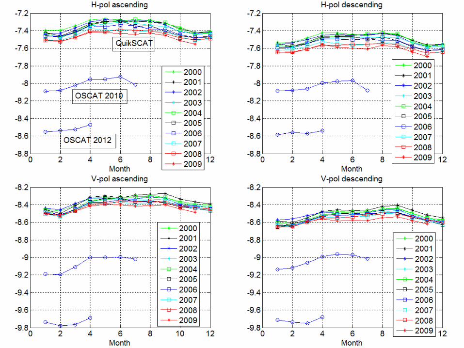
QuikSCAT and ECMWF retrieved wind speed versus time

• Yearly average of wind speed

• -60 < lat <60• QuikSCAT shows no

trend in wind• ECMWF shows

increasing wind speed

Part 2: OSCAT stability evaluation using land targets

2-1: OSCAT backscatter for the same time of year – Characteristic of difference versus signal level– Variation of difference as a function of time

2-2: Comparison with repointed QuikSCAT backscatter2-3: Seasonal adjust using QuickSCAT data

– Variation of difference as a function of time

2-1: OSCAT stability for the same time of year

• Use land, spatial and time mask– Kp_spat and Kp_time < 0.1

• At these location, calculate average sigma0 in dB scale

• Histogram of backscatter difference• Backscatter difference vs backscatter level

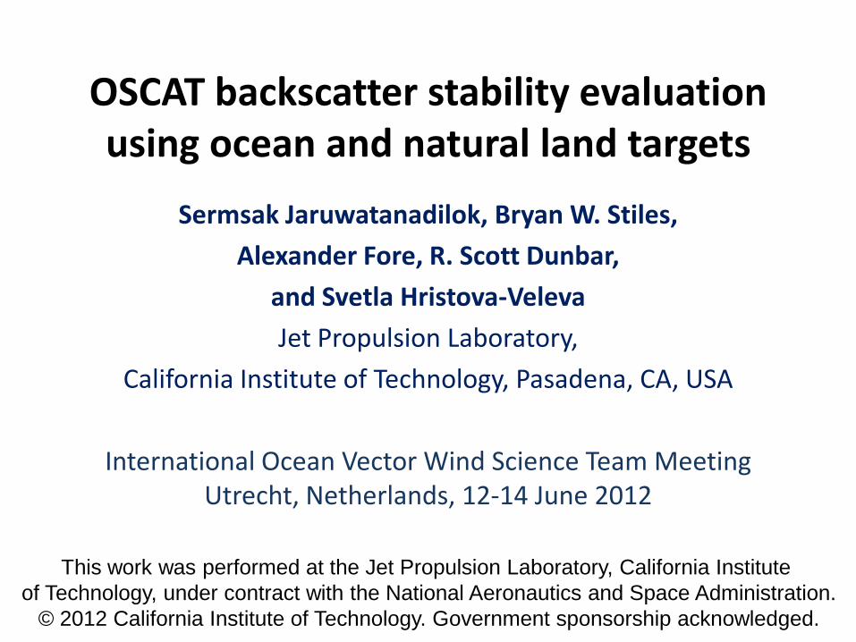
OSCAT backscatter difference Jan 2012 (dB) – Jan 2010 (dB)

• Lots of negatives

Average all data = -0.4884 dB

• OSCAT H-pol January backscatter difference (2012-2010)

• OSCAT V-pol January backscatter difference (2012-2010)

Average difference = -0.6114 dB

OSCAT backscatter level difference (2012-2010) as a function of month

H-pol Asc aft Asc fore Des aft Des for Average

January -0.4884 -0.4653 -0.4963 -0.5014 -0.4879

February -0.4670 -0.4572 -0.5095 -0.5200 -0.4884

March -0.4590 -0.4691 -0.4949 -0.5149 -0.4845

April -0.5148 -0.5161 -0.5143 -0.5477 -0.5232

May -0.5183 -0.5265 -0.5323 -0.5720 -0.5373

V-pol Asc aft Asc fore Des aft Des for Average

January -0.6114 -0.5804 -0.6052 -0.5994 -0.5991

February -0.5876 -0.5631 -0.6316 -0.6320 -0.6036

March -0.5805 -0.5818 -0.6205 -0.6266 -0.6024

April -0.6482 -0.6520 -0.6420 -0.6517 -0.6485

May -0.6718 -0.6625 -0.6791 -0.6891 -0.6756

2-2: OSCAT versus Rep QuikSCAT • QuikSCAT is commanded to point to OSCAT – V-pol incidence

angle on day 82, 2012• Use data on day 82-107 (March 22 – April 16)• For same time of year

– Evaluate difference of OSCAT backscatter for 2012 and 2010– Evaluate difference of QuikSCAT backscatter for 2012 and 2011

METHOD• Pick sigma0 from stable and homogeneous locations• Use only OSCAT data with the same look geometry as

Repointed QuikSCAT • Evaluate drift by taking the difference in sigma0 in dB scale

from one year to another• Only evaluate at co-location points

2-3: Drift versus time – seasonal adjusted

• Use 2000 – 2008 QuikSCAT (spinning) to obtain seasonal trend– Average monthly for all 9 years => result is average

monthly sigma0 for the whole year– Use January as reference, backscatter difference from

other months are “seasonally” adjusted• Apply seasonal adjustment to the OSCAT data• Behavior of OSCAT backscatter versus time• Note: Spinning QuikSCAT data has different incidence angle

than that of OSCAT so seasonal change of OSCAT backscatter are somewhat different (more). We use spinning QuikSCAT because we have a long-term data record.

Seasonal adjust number

• Magnitude is less than 0.15 dB

Jan 2010

July 2011

Jan 2012 Missing months ?

Missing months ?

Part 3: OSCAT stability evaluation using ocean data

• For both repointed QuikSCAT and OSCAT data– Pick only ocean data, abs(latitude) < 50 degree

• For OSCAT data– Pick only scan position 100 for H-pol, 101 for V-pol – Use high gain slices (slice #4 for Hpol #6 for Vpol)

• Method– Bin data versus footprint matched ECMWF speed

and relative azimuth

mean(difference in dB)

QuikSCAT V-pol -0.0539 dB / 1 year

OSCAT V-pol -0.6498 dB / 2 years

OSCAT H-pol -0.622 dB / 2 years

January February March April May

QS V-pol -0.0159 -0.0539 0.0058

Ocean OSCAT V-pol -0.5803 -0.6421 -0.5355 -0.6498 -0.6349

Ocean OSCAT H-pol -0.5359 -0.5724 -0.4858 -0.6222 -0.5117

Land OSCAT V-pol -0.5991 -0.6036 -0.6024 -0.6485 -0.6756

Land OSCAT H-pol -0.4879 -0.4884 -0.4845 -0.5232 -0.5373

Sigma0 difference (dB) for the same month

2012-2011

2012-2010

Average backscatter versus timeECMWF: 5 <= speed <10

Conclusions• Land and ocean are used in evaluating OSCAT backscatter• It shows that there is definitely a drop in OSCAT backscatter

in the order of 0.5 dB in H-pol and 0.6 dB in V-pol in two year time span

• The characteristics of OSCAT backscatter drop is still under investigation. More data is needed, especially, the missing August 2010 – June 2011

• We will continue monitor and characterize this OSCAT backscatter behavior as long as we receive OSCAT data and QuikSCAT is still operating

• Because of its stability, QuikSCAT provides crucial information about any geophysical change which is linked to proper OSCAT backscatter calibration

BACKUP

Absolute calibration check• The absolute calibration to be applied is adding 0.3362 dB for H-pol and

0.2255 dB for V pol to the previous sigma0 data• Check by looking at exact same sigma0 location in the exact same rev:

“S1L1B2010094_02802_02803.h5”• Examples: σo(10,20,4) denote σo at scan position 10, orbit position 20, slice

number 4H-pol=> new σo(10,20,4) = -12.1453 old σo (10,20,4) = -12.4900 difference = 0.3447V-pol=> new σo(10,20,4) = -12.3717 old σo (10,20,4) = -12.6000 difference = 0.2283

• The difference is NOT exactly, but that is expected because of quantization issue.

• When looking at all data in the file, we found that there are some points where the differences are much larger than this absolute calibration.

• Note: The number of orbit step in new data is different from the old ones in some of the files. For 6 revs we received, only 2 has the same number of orbit step as those of old files.

Difference in new and old files

• Processed file : S1L1B2010094_02802_02803.h5• Pick good sigma0 data • Mean of the difference V-pol =0.2205 dB H-pol=0.3312 dB

There are a few points where differences are large

Potential land targets 2

• Specific 1 by 1 degree box with smallest time variation in the regions

• Variation Kp = std()/mean() in linear scale

Amazon Antarctica Australia Congo Indonesia Greenland SaharaLocation of center of box

(Lat,Lon)N 5.3W 59.2

S 75.1E 123.1

S 23.5E 142.7

S 0.2E 11.2

S 6.0E 139.5

N 73.5W 37.5

N 27.2E 17.8

Averageσo (dB)

H-pol asc -6.891 -6.610 -11.380 -7.373 -7.106 -8.466 -10.346H-pol des -7.123 -6.631 -11.218 -7.553 -7.396 -8.457 -10.344V-pol asc -8.114 -7.441 -13.133 -8.607 -8.564 -8.297 -11.977V-pol des -8.428 -7.459 -12.912 -8.988 -8.847 -8.303 -11.973

Variation(Kp)

H-pol asc 0.0255 0.0275 0.0444 0.0181 0.0299 0.0485 0.0276H-pol des 0.0194 0.0282 0.0436 0.0193 0.0192 0.0481 0.0233V-pol asc 0.0256 0.0243 0.0443 0.0200 0.0330 0.0414 0.0288V-pol des 0.0165 0.0239 0.0447 0.0189 0.0169 0.0405 0.0213

Amzlim=[ 4.8 5.8 300.3 301.3];

Kp Sigma0 (dB)

V pol 0.0422 -8.2677

V pol aft 0.0399 -8.2918

V pol for 0.0438 -8.2438

V pol ascending 0.0256 -8.1135

V pol ascending aft 0.0245 -8.1471

V pol ascending for 0.0243 -8.0802

V pol descending 0.0165 -8.4276

V pol descending aft 0.0163 -8.4414

V pol descending for 0.0161 -8.4138

H pol 0.0351 -7.0055

H pol aft 0.0325 -7.0251

H pol for 0.0370 -6.9860

H pol ascending 0.0255 -6.8913

H pol ascending aft 0.0214 -6.9154

H pol ascending for 0.0280 -6.8674

H pol descending 0.0194 -7.1228

H pol descending aft 0.0184 -7.1376

H pol descending for 0.0197 -7.1079

Antlim=[-75.6 -74.6 122.6 123.6];

Kp Sigma0 (dB)

V pol 0.0242 -7.4500

V pol aft 0.0203 -7.5073

V pol for 0.0204 -7.3934

V pol ascending 0.0243 -7.4412

V pol ascending aft 0.0199 -7.5027

V pol ascending for 0.0198 -7.3805

V pol descending 0.0239 -7.4588

V pol descending aft 0.0208 -7.5119

V pol descending for 0.0205 -7.4063

H pol 0.0280 -6.6205

H pol aft 0.0275 -6.6568

H pol for 0.0260 -6.5844

H pol ascending 0.0275 -6.6103

H pol ascending aft 0.0273 -6.6426

H pol ascending for 0.0259 -6.5784

H pol descending 0.0282 -6.6306

H pol descending aft 0.0274 -6.6711

H pol descending for 0.0261 -6.5905

Kp Sigma0 (dB)

V pol 0.0409 -8.3001

V pol aft 0.0403 -8.3162

V pol for 0.0413 -8.2841

V pol ascending 0.0414 -8.2973

V pol ascending aft 0.0401 -8.3343

V pol ascending for 0.0411 -8.2606

V pol descending 0.0405 -8.3029

V pol descending aft 0.0402 -8.2981

V pol descending for 0.0409 -8.3076

H pol 0.0482 -8.4614

H pol aft 0.0488 -8.4772

H pol for 0.0475 -8.4456

H pol ascending 0.0485 -8.4656

H pol ascending aft 0.0480 -8.5218

H pol ascending for 0.0457 -8.4101

H pol descending 0.0481 -8.4572

H pol descending aft 0.0475 -8.4331

H pol descending for 0.0481 -8.4814

Greenland [73.0 74.0 322.0 323.0]

Kp Sigma0 (dB)

V pol 0.0480 -8.7933

V pol aft 0.0465 -8.8047

V pol for 0.0493 -8.7819

V pol ascending 0.0200 -8.6073

V pol ascending aft 0.0190 -8.6256

V pol ascending for 0.0202 -8.5892

V pol descending 0.0189 -8.9876

V pol descending aft 0.0200 -8.9916

V pol descending for 0.0178 -8.9835

H pol 0.0447 -7.3726

H pol aft 0.0435 -7.3871

H pol for 0.0458 -7.3582

H pol ascending 0.0181 -7.1997

H pol ascending aft 0.0171 -7.2193

H pol ascending for 0.0180 -7.1802

H pol descending 0.0193 -7.5527

H pol descending aft 0.0198 -7.5616

H pol descending for 0.0187 -7.5439

Conlim=[ -0.7 0.3 10.7 11.7];

Kp Sigma0 (dB)

V pol 0.0253 -11.9750

V pol aft 0.0247 -12.0029

V pol for 0.0243 -11.9472

V pol ascending 0.0288 -11.9766

V pol ascending aft 0.0224 -12.0556

V pol ascending for 0.0225 -11.8990

V pol descending 0.0213 -11.9733

V pol descending aft 0.0208 -11.9508

V pol descending for 0.0206 -11.9960

H pol 0.0254 -10.3450

H pol aft 0.0251 -10.3634

H pol for 0.0251 -10.3266

H pol ascending 0.0276 -10.3460

H pol ascending aft 0.0215 -10.4207

H pol ascending for 0.0219 -10.2724

H pol descending 0.0230 -10.3440

H pol descending aft 0.0212 -10.3068

H pol descending for 0.0216 -10.3814

Sahlim=[ 26.7 27.7 17.3 18.3]

Small region check

• Backscatter image at several regions• Drift of backscatter at one by one degree box

Amazon Antarctica Congo Greenland SaharaLocation of center of

the box (Lat,Lon)N 5.3W 59.2

S 75.1E 123.1

S 0.2E 11.2

N 73.5W 37.5

N 27.2E 17.8

Drift (dB) H-pol -0.51 -0.632 -0.4090 -0.373 -0.7146

V-pol -0.6254 -0.7130 -0.6201 -0.6284 -0.6730

Amazon box – H-polCenter of the box: N 5.3 W 59.2

Mean drift in box = -0.51 dB

Amazon box – V polCenter of the box: N 5.3 W 59.2

Mean drift in box = -0.6254 dB

Average sigma0 (in linear scale) versus time

6 <= speed <7 200<= relative azimuth <210