OTTO VON-GUERICKE-UNIVERSITY MAGDEBURG · 1 Introduction Earnings of foreigners have been...

Language Usage, Participation, Employment and Earnings

Alisher Aldashevy Johannes Gernandt Stephan L. Thomsen

FEMM Working Paper No. 18, September 2007

OTTO-VON-GUERICKE-UNIVERSITY MAGDEBURG FACULTY OF ECONOMICS AND MANAGEMENT

Otto-von-Guericke-University Magdeburg Faculty of Economics and Management

P.O. Box 4120 39016 Magdeburg, Germany

http://www.ww.uni-magdeburg.de/

F E M M Faculty of Economics and Management Magdeburg

Working Paper Series

Language Usage, Participation, Employment and

Earnings∗

Evidence for Foreigners in West Germany with Multiple Sources of Selection

Alisher Aldashev†, Johannes Gernandt‡ and Stephan L. Thomsen§

†,‡ ZEW, Mannheim§ OvG-University, Magdeburg

November 5, 2007

Abstract

Language ability may not only affect the earnings of the individual, but the probability to participate in thelabor market or becoming employed as well. It may also affect selection of people into economic sectors andoccupation. In this paper the effects of language ability on earnings are analyzed for foreigners in Germanywith joint consideration of up to four types of self-selection. The results show that language proficiencysignificantly increases participation and employment probability and affects earnings directly. However,when self-selection into economic sectors and occupation is regarded, the direct effects of language abilityon earnings vanish.

Keywords: Foreigners, Participation, Employment, Language Ability, Multiple SelectionJEL Classification: J61, I12, J15

∗The authors thank Julia Horstschraer and Thomas Walter for valuable comments and Philipp Eisenhauer andCarmen Nagy for their research assistance. This paper is part of ZEW project “Returns to Education and WageInequality for Persons with Migration Background in Germany”. The usual disclaimer applies.†Alisher Aldashev is Research Fellow at the Centre for European Economic Research (ZEW), Mannheim, e-mail:

[email protected].‡Johannes Gernandt is Research Fellow at the Centre for European Economic Research (ZEW), Mannheim,

e-mail: [email protected].§Stephan L. Thomsen (corresponding author) is Assistant Professor of Labor Economics at Otto-von-Guericke-

University Magdeburg, Department of Economics and Management. P.O. BOX 4120, D-39016 Magdeburg, e-mail:[email protected], phone: +49 391 67-18431, fax: +49 391 67-11218.

1 Introduction

Earnings of foreigners have been extensively studied since the seminal paper of Chiswick (1978).

A well-established finding of most of the works is that migrants’ earnings usually lack behind

those of the equally-qualified and experienced native population, catching up at a later stage. One

explanation for this gap are language difficulties of the migrants. There is a vast international

evidence that speaking the language of the host country fluently has significant positive effects on

earnings, see, e.g., Chiswick, Lee, and Miller (2005) for Australia, Chiswick and Miller (1999) for the

United States, Shields and Price (2002) for the United Kingdom, Berman, Lang, and Siniver (2000)

for Israel, and Dustmann and van Soest (2002) for Germany among others.1 However, evaluating

the impact of language ability on earnings may be complicated for the following reasons: First, self-

selection issues may play an important role for migrants’ earnings. For example, Chiswick, Lee, and

Miller (2005) show that controlling for self-selection may weaken the significance of the language

variable. Language ability may also affect the participation decision and occupation choice. In

that sense, even in the absence of wage discrimination due to language proficiency there could be

discrimination in terms of labor market participation, employment or choice of economic sector and

occupation. Neglecting those aspects when analyzing the impact of language ability on earnings

might lead to severely biased estimates. A second complication may arise from measurement or

misclassification errors in the language ability variable. In most surveys, people are asked to self-

assess the language fluency. Hence, inter-personal (and even intra-personal) comparability may be

limited, see, e.g., Dustmann and van Soest (2001).

The purpose of this paper is to analyze the impact of language ability on earnings for foreigners.

In the theoretical model individuals with better language skills are more likely to participate and

to be employed even in the absence of a language premium in wages. Moreover, more proficient

individuals end up working in higher-paying firms. In this paper, we consider the different stages

of self-selection explicitly. Namely, we take account of self-selection into the labor market as well

as self-selection into employment. As both decisions may be correlated we estimate both decisions

simultaneously in a first step. However, modeling selection into employment as a whole may veil

potentially relevant patterns of economic sector and occupation choice. Therefore, in an extension

of the model we estimate the effect of language ability on earnings regarding self-selection into

economic sectors and occupation.

For the empirical application, data from eight waves of the German Socio-Economic Panel (GSOEP)

for the years 1996 to 2005 (excluding the years 2002 and 2004 due to missing information on lan-

guage usage) are used. All persons with a foreign citizenship are considered in the analysis and

estimations are carried out for the full sample.2 However, a rising number of people possessing1 For further evidence the interested reader is referred to the overview by Chiswick and Miller (1995) and the

studies by McManus, Gould, and Welch (1983), Chiswick (1991) and Dustmann and van Soest (2001).2 The analysis has to be limited to foreigners since further groups with migration background are not asked about

their language usage in GSOEP. However, only about half of the people with migration background living in Germanyare foreigners. For this reason, additional information would be of great value for future research, see e.g. Aldashev,Gernandt, and Thomsen (2007).

2

foreign citizenship is born in Germany (so-called second generation). To test the sensitivity of

the estimates of language usage we carry out separate estimations for first and second generation

foreigners in addition. To mitigate problems of measurement error in the language ability vari-

able, we use information on language usage in the household as a proxy for individual language

command.

Our empirical results show that language proficiency significantly increases participation and em-

ployment probability of foreigners in Germany. Moreover, earnings are clearly higher for persons

speaking mainly or at least partly German in the household compared to people using the native

language only. When additional selection into economic sector and type of occupation is consid-

ered, language usage appears to be relevant for both choices as well. However, the direct effect

of language usage on earnings becomes insignificant. For that reason, we conclude that language

ability is an important determinant for the selection processes in the labor market, but there is no

discrimination in earnings associated with it.

The paper is organized as follows: Section 2 presents the theoretical model with flat wages within

each firm. Section 3 discusses selection issues and the econometric model. Details on the data

and some selected descriptives are given in section 4. The empirical estimates of language usage,

participation, employment and earnings are discussed in section 5. The final section concludes.

2 Theoretical Background

The central question of the paper is the effect of language proficiency on earnings, participation

and employment. We assume here that language ability is related to productivity and through this

affects earnings, participation and employment. The variant of the Burdett and Mortensen (1998)

model (see also Manning, 2003, Mortensen, 2003) laid out in this section provides argumentation

for controlling for self-selection even if an employer pays the same wage for workers with different

language abilities.

Consider an economy consisting of three types of individuals with productivities p0, p1, and p2,

such that p0 < p1 < p2. Suppose that there is a guaranteed minimal income b (for example social

or welfare assistance). The lowest possible wage a firm can set is thus b. Suppose that p0 < b. This

implies that no firm employs individuals with productivity p0 and they do not participate.3 The

inflow of job offers to unemployed workers happens in continuous time according to a stationary

Poisson process so that each worker receives only one offer at maximum during an infinitesimal

time interval. Employed workers may search on the job for higher paid vacancies. The arrival

rates of job offers to employed and unemployed workers are assumed to be equal. Since the arrival

rates are the same for out-of-job and on-the-job search, it is optimal for a worker to accept the3 This is simplification. In reality, some unproductive workers would still participate to be eligible to receive

unemployment assistance. However, one should then consider that participation is associated with a cost (cost oftime-inflexibility due to being available to the labor market). So in the end, there would still be non-participantsfor whom the net effect of participation is negative.

3

first offer she receives and to continue searching on the job for a better offer (if returns to search

are higher than the search costs). As a result in equilibrium there will still be a fraction of highly

productive workers employed at low-wage firms.

For simplicity, suppose that there is a flat wage policy in any firm, so that a firm that hires both

p1 and p2 workers pays equal wages to them. A firm offering a wage lower than p1 can hire both p1

and p2 individuals, but a firm with a wage above p1 can hire only p2 workers. Consider an arbitrary

firm 1, which offers a wage equal to b and has a profit of π1 = (p1 − b)L1(p1) + (p2 − b)L1(p2),

where L1(p1) is the labor supply of p1 workers to firm 1 and L1(p2) is the labor supply of p2

workers to firm 1. A firm 2, offering a wage w greater than p1, has a profit of π2 = (p2−w)L2(p2),

where L2(p2) is the labor supply of p2 workers to firm 2. Then, as in a Burdett and Mortensen

(1998) model, there exists an equilibrium such that both firms are equally profitable. Firm 2 pays

a higher wage, but at the same time has a larger workforce of p2 workers as it would “steal away”

some of the workers from firm 1 attracted by a higher wage. Ultimately, more p2 workers would

be concentrated in high-wage firms.

The model implies that even in the presence of a flat wage policy within a firm the observed wages

in the sample between p1 and p2 workers would be different due to differences in employment

probabilities. When estimating the effect of p on wages one has to keep in mind that p1 workers

are more likely to be unemployed than p2 workers. Moreover, participation rates differ with p as

p0 individuals do not participate. This implies that the estimated effect of p on wages based on the

sample of employed individuals is biased as the sample of employed wage-earners is self-selected

and a distribution of p from a sample of employed individuals is not a correct estimate of the

distribution of p from the population.

3 Econometric model and selection issues

To estimate the effect of language proficiency on earnings, we assume language proficiency to be

related to productivity as

p = ψ(H) + υ, (1)

where H is language proficiency, ψ is some arbitrary function and υ includes other factors affecting

productivity. The theoretical model is constructed in such a way to allow a flat-wage policy, i.e.

a firm pays the same wage to workers with different productivities. In the empirical sense this

implies that we assume firms do not discriminate workers by language proficiency with respect to

earnings. However, discrimination with respect to employment might be present.

Thereby, we would expect a higher participation probability and higher employment chances of

foreigners with better language command. On the other hand, according to theory, there is a

critical level of productivity for participation, b. Persons with productivity below this value do

not participate. Therefore, the participating individuals with a good language command could

have lower values of υ as higher values of H compensate for this to reach the critical level of

4

productivity. Moreover, one needs to keep in mind that the most productive workers are more

likely to be employed in high-paid firms raising out another source of self-selection.

This implies that the effect of language ability on wages could be overestimated when the self-

selection is not accounted for. In the theoretical model it was shown that the samples of participat-

ing and employed individuals may be non-random. To estimate the earnings equation controlling

for self-selection we need to model the participation and employment decisions simultaneously. To

do so, we use a variant of the well-known Heckman-Lee method.4

The participation equation is given as:

I∗1 = Z1γ1 + ε1, (2)

where Z1 is a matrix of exogenous variables, γ1 is a parameter vector, and ε1 is a random compo-

nent. I∗1 is latent, instead we observe I1 = 1 (in case of participation) if wR > b and I1 = 0 (for

nonparticipating individuals) otherwise where wR means reservation wage.

The employment equation is given as:

I∗2 = Z2γ2 + ε2, (3)

where Z2 is a matrix of exogenous variables, γ2 is a parameter vector, and ε2 is a random compo-

nent. I∗2 is latent, instead we observe I2 = 1 (in case of employment) if w > wR and I2 = 0 (for

unemployed individuals) otherwise.

Both I∗1 and I∗2 depend on the reservation wage. If Z1 and Z2 contain all variables which determine

wR, ε1 and ε2 are independent. If some of these variables are not observed (or not contained) in

the data they will be included in the error term, which could result in the correlation between ε1

and ε2. Hence, it might be advisable to allow for this correlation and estimate equations 2 and 3

jointly.

Finally, the wage offer equation is of a standard Becker-Mincer type:

w = Xβ + u, (4)

where X is a matrix of exogenous variables, β is a parameter vector, w is a log wage, and u is

an error component, which is normally distributed with mean zero. Wages are observed if both

I1 = 1 and I2 = 1. Hence, expected observed wage is given by:

E(w|I1 = 1, I2 = 1) = Xβ + E(u|I1 = 1, I2 = 1). (5)

Define the covariance between the error terms of the participation and the earnings equation as

σu1 = cov(u, ε1), and analogously between employment and earnings σu2 = cov(u, ε2). Moreover,4 The classical Heckman-Lee method, following to Heckman (1976) and Lee (1976), is applied when one source

of self-selection is present. In our case we have two (participation and employment), hence, certain adjustments arenecessary, which are discussed later in this section.

5

let var(u) = σ2u. In order to estimate the selection model, variances of the error terms have to

be standardized as var(ε1) = var(ε2) = 1 and cov(ε1, ε2) = ρ. Following Mohanty (2001) (see also

Maddala, 1983), E(u|I1 = 1, I2 = 1) = σu1λ1 + σu2λ2, where λ1 = φ(Z1γ1)Φ(A)/F (Z1γ1, Z2γ2; ρ)

and λ2 = φ(Z2γ2)Φ(B)/F (Z1γ1, Z2γ2; ρ), A = (Z2γ2 − ρ · Z1γ1)/√

(1− ρ2), B = (Z1γ1 − ρ ·Z2γ2)/

√(1− ρ2). φ is the univariate standard normal density function, Φ is the univariate stan-

dard normal distribution function, and F is the bivariate standard normal distribution function.

It is worth noting that the λs are the familiar inverse Mill’s ratios adjusted for the bivariate

case. In fact, if participation and employment decisions are unrelated then F (Z1γ1, Z2γ2; ρ) =

Φ(A) ·Φ(B) (conditional probability of independent events) and hence λ1 = φ(Z1γ1)/Φ(Z1γ1) and

λ2 = φ(Z2γ2)/Φ(Z2γ2), which are the inverse Mill’s ratios in a standard two-stage Heckit model,

see Heckman (1979).

The conditional wage in equation 5 can be rewritten as:

E(w|X) = Xβ + λ1σu1 + λ2σu2. (6)

To estimate equation 6, in a first step equations 2 and 3 have to be estimated jointly. Estimates

obtained at the first stage (γ1, γ2, ρ) are used to construct λ1 and λ2 as defined above. At the

second stage wage is regressed on X, λ1 and λ2 by OLS (as in the Heckman-Lee method), which

produces the parameter estimates β, σu1, and σu2.

4 Data and Descriptives

4.1 Dataset

To analyze the effect of language ability on earnings, labor market participation and employment

we use data on foreigners in West Germany from eight waves of the German Socio-Economic Panel

(GSOEP) for the years 1996 to 2005 excluding 2002 and 2004 due to missing information on the

variable of interest (language usage at home). GSOEP is a wide-ranging representative longitudinal

study of private households carried out since 1984 in Germany. It provides information about all

household members covering Germans, foreigners and recent immigrants to Germany. In 2005,

there were almost 12,000 households and more than 21,000 persons sampled in GSOEP.5 GSOEP

is preferable to other data sources in Germany for our purpose because it is not restricted to

certain labor market groups, e.g. unemployed persons or people registered in the social security

system. Moreover, second generation foreigners, i.e. persons who were born in Germany, possess

German citizenship and whose parents immigrated to Germany from abroad, can be identified. In

addition to the full sample of foreigners we will carry out separate estimations for first and second

generation migrants to enable a more comprehensive analysis on the role of language proficiency.

Variables for language proficiency are prone to measurement error due to self-assessment of the

respondents in many surveys. For example, Dustmann and van Soest (2001) show that reliability5 For more information, see, e.g., Haisken-DeNew and Frick (2005).

6

of the language proficiency variable in GSOEP may be limited in terms of inter-personal and

intra-personal comparability. The language spoken in the household is also not free from inter-

personal variation. However, in about half of observations for foreigners the language ability

is not reported, which makes language spoken in the household preferable for our analysis not

to significantly reduce the sample size of foreigners. Raw descriptive statistics reveal a strong

relationship between language proficiency and language usage in the household, suggesting that

language spoken in the household could be a good proxy for language proficiency. For example, 57

percent of people who speak mainly German at home report to have “very good” speaking ability

(in German), more than 90 percent report at least “good” speaking ability. More than 40 percent

of those who speak partly German at home report to have “good” speaking ability and over 30

percent report “satisfactory” speaking ability. Persons speaking mostly mother tongue at home

mostly report “satisfactory” (about 40%) and “poor” (about 35%).

This variable categorizes language use of the respondents into three categories: speaking mainly

German, speaking mainly the language of the home country or speaking partly German and partly

the mother tongue. As it could be expected that reporting the type of the language used in the

household is easier than assessing language proficiency in terms of written or oral skills, we suppose

the variable to be much less prone to measurement errors.6

As mentioned above, GSOEP provides information on labor market states of non-participation,

employment and unemployment. Moreover, information on employment is not limited to jobs sub-

ject to social security contributions, but also covers civil servants and self-employed. It also covers

details about part-time, full-time employment or whether the individuals has a minor job only.

Unfortunately, even with this information at hand, modeling the two-stage self-selection process

requires some further treatment of the variables. Respondents are asked two separate questions,

whether they are registered unemployed and whether they are non-participants. However, non-

participation is not necessarily understood by respondents as being out of the labor market in an

economic sense (some people mix up non-participation and registered unemployment). For that

reason, we define people as non-participants if they responded “not in the labor market” and “not

registered as unemployed” simultaneously. It has to be noted that this group might still include

some active participants who are not registered at the labor office.7 A further complication arises

from the fact that respondents do not necessarily understand employment and unemployment as

exclusive labor market states. For example, a person having a low-paid job8 is eligible for receiving

additional subsistence allowance. Officially registered unemployed are allowed to hold a minor job

or work part-time and earn up to a certain threshold. In the empirical application, unemployed

people who are registered at the labor office but earn more than 1,000 Euro per month are counted

as employed. The outcome variable (real gross hourly wage) is obtained for all employees including

the self-employed by dividing the gross earnings in the month prior to the interview by the reported6 It may be useful to note that on average about two thirds to three quarters of the respondents answer equally

in consecutive waves. Moreover, there is no reason to expect “changers” to correct wrong answers, but to reportchanges in language usage that actually occurred.

7 Potential reasons could be, for example, expiration of unemployment benefits eligibility or benefit sanctions.8 with earnings below the subsistence level

7

working hours of the last week that are extrapolated to monthly hours. Wages are deflated using

the consumption price index based on the year 2000 to get real consumption wages of comparable

purchasing power.9

Furthermore, the sample is restricted to foreigners who arrived in West Germany after 1948.

German resettlers possessing foreign citizenship are excluded from the analysis. Moreover, due

to sample size considerations, workers in the agricultural sector are dropped. For reasons of

homogeneity, we only consider people aged 25 to 55 years to avoid bias due to education or early

retirement decisions (those in education are explicitly discarded from our data). Individuals who

do not report the language usage in the household are excluded from the sample (less than 2

percent). Finally, information on wages is symmetrically two percent trimmed to exclude extreme

values. In GSOEP, foreigners could leave the sample for two reasons. First, there is some common

panel mortality, i.e. persons decide not to participate in subsequent interviews or they change their

place of residence and interviewers lose track of them. Second, foreigners could be naturalized.

Assuming that panel mortality in GSOEP is random, naturalization could be assumed to be non-

random. In the data, 201 foreigners out of 2,230 became Germans during the observation period.

Performing distribution tests of equality of language usage for “changers” and “non-changers”

showed no significant differences. Hence, we could refrain for controlling for selection into German

citizenship explicitly in the analysis.10

4.2 Selected Descriptives

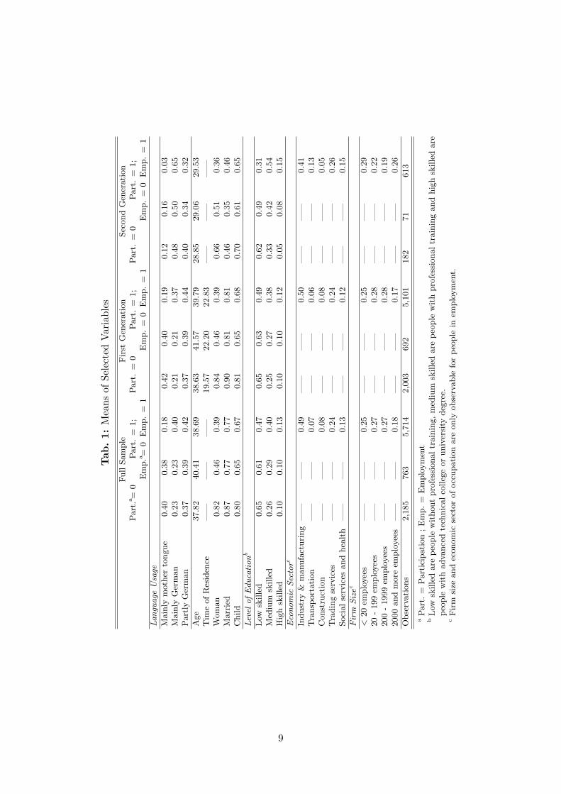
Before presenting the empirical application and the estimation results, it is useful to take a closer

look on the data available. Table 1 provides means of selected variables used in the empirical models

with a distinction between full sample (left panel) and first (center) and second generation (right

panel) foreigners. Each panel contains three columns, of which the left one provides information on

non-participants in the labor market, the center one for participants who are unemployed and the

right column refers to means for the sample of employed foreigners. As becomes obvious from the

table, the sample for the second generation is quite small compared to that of the first generation.

Hence, results for the full sample in analysis are strongly determined by the first generation.

Instead of discussing the single figures in the table, we will concentrate on findings that are mean-

ingful for our analysis. First, compared to the other groups employed individuals are more likely

to speak mainly German at home than their mother tongue. Whereas about 40 percent of the

group of non-participants speak the language of their home country at home, in the group of the

employed the share is about 18 percent only (for the full sample). Regarding the results for the

first and second generation, this discrepancy is more pronounced in the parents’ generation. People

of the second generation use German far more frequently at home.9 It should be noted that the reported gross earnings in the month prior to the interview have not been adjusted

for end-of-year bonuses, overtime-payments, holiday allowances etc.10 It should be noted that persons who were naturalized are not considered in the estimations after the date of

naturalization.

8

Tab

.1:

Mea

nsof

Sele

cted

Var

iabl

es

Full

Sam

ple

Fir

stG

ener

ati

on

Sec

ond

Gen

erati

on

Part

.a=

0P

art

.=

1;

Part

.=

0P

art

.=

1;

Part

.=

0P

art

.=

1;

Em

p.a

=0

Em

p.

=1

Em

p.

=0

Em

p.

=1

Em

p.

=0

Em

p.

=1

La

ngu

age

Usa

ge

Main

lym

oth

erto

ngue

0.4

00.3

80.1

80.4

20.4

00.1

90.1

20.1

60.0

3M

ain

lyG

erm

an

0.2

30.2

30.4

00.2

10.2

10.3

70.4

80.5

00.6

5P

art

lyG

erm

an

0.3

70.3

90.4

20.3

70.3

90.4

40.4

00.3

40.3

2

Age

37.8

240.4

138.6

938.6

341.5

739.7

928.8

529.0

629.5

3T

ime

of

Res

iden

ce—

——

——

—19.5

722.2

022.8

3—

——

——

—W

om

an

0.8

20.4

60.3

90.8

40.4

60.3

90.6

60.5

10.3

6M

arr

ied

0.8

70.7

70.7

70.9

00.8

10.8

10.4

60.3

50.4

6C

hild

0.8

00.6

50.6

70.8

10.6

50.6

80.7

00.6

10.6

5

Lev

elo

fE

du

cati

on

b

Low

skille

d0.6

50.6

10.4

70.6

50.6

30.4

90.6

20.4

90.3

1M

ediu

msk

ille

d0.2

60.2

90.4

00.2

50.2

70.3

80.3

30.4

20.5

4H

igh

skille

d0.1

00.1

00.1

30.1

00.1

00.1

20.0

50.0

80.1

5

Eco

no

mic

Sec

torc

Indust

ry&

manufa

cturi

ng

——

——

0.4

9—

——

—0.5

0—

——

—0.4

1T

ransp

ort

ati

on

——

——

0.0

7—

——

—0.0

6—

——

—0.1

3C

onst

ruct

ion

——

——

0.0

8—

——

—0.0

8—

——

—0.0

5T

radin

gse

rvic

es—

——

—0.2

4—

——

—0.2

4—

——

—0.2

6Soci

al

serv

ices

and

hea

lth

——

——

0.1

3—

——

—0.1

2—

——

—0.1

5

Fir

mS

izec

<20

emplo

yee

s—

——

—0.2

5—

——

—0.2

5—

——

—0.2

920

-199

emplo

yee

s—

——

—0.2

7—

——

—0.2

8—

——

—0.2

2200

-1999

emplo

yee

s—

——

—0.2

7—

——

—0.2

8—

——

—0.1

92000

and

more

emplo

yee

s—

——

—0.1

8—

——

—0.1

7—

——

—0.2

6

Obse

rvati

ons

2,1

85

763

5,7

14

2,0

03

692

5,1

01

182

71

613

aP

art

.=

Part

icip

ati

on

;E

mp.

=E

mplo

ym

ent

bL

owsk

ille

dare

peo

ple

wit

hout

pro

fess

ional

train

ing,

med

ium

skille

dare

peo

ple

wit

hpro

fess

ional

train

ing

and

hig

hsk

ille

dare

peo

ple

wit

hadva

nce

dte

chnic

al

colleg

eor

univ

ersi

tydeg

ree.

cF

irm

size

and

econom

icse

ctor

of

occ

upati

on

are

only

obse

rvable

for

peo

ple

inem

plo

ym

ent.

9

Another finding worth to mention refers to gender differences between the three different labor

market states. The vast majority of non-participating foreigners in Germany are women (82

percent). Within the sample of participants, the share of women is clearly lower. Within the

group of unemployed foreigners, about 46 percent and in the group of employed persons only 39

percent are females. Including the distinct results for first and second generation foreigners, the

picture does not change by far. Even though inactivity of women of the first generation is a bit

more pronounced, also for the second generation the share of females in that group is about two

thirds.

We consider the level of education in three different categories. The low-skilled are people who

lack professional training. This group should be expected to be most strongly disadvantaged in

the labor market, in particular in a highly developed country with a regulated labor market as

Germany. Medium-skilled comprises people who finished a professional training (not necessarily in

the German apprenticeship system, but comparable to it). Finally, the high-skilled are those who

graduated from advanced technical college (Fachhochschule) or university. The shares of the low-

skilled are particularly large in the group of non-participants (about 65 percent of that group) and

the group of unemployed persons (about 61 percent). In contrast, less than half of the employed

persons are low skilled (47 percent). Although the share of low-skilled is smaller in the group of

employed it is still considerable. However, as many un- and low-skilled foreigners were recruited

during the 1960s and early 1970s to reduce labor supply shortage this result is not surprising.

In contrast, the qualification of the second generation is on average higher. For this group, the

majority of the employed is at least medium-skilled, while the number of low-skilled is less than

one third.11

The last point we want to discuss is the selection into economic sectors. Naturally, this information

is only observable for people who are actually employed. The figures from Table 1 clarify the

generational differences. Whereas more than half of the first generation (and, therefore, the full

sample) work in industry and about one quarter in trading services, the composition has changed

slightly in the second generation. Here, the share of people employed in industry is still high with

about 41 percent, but lower than in their parents’ generation. Though the proportion working in

trading services is comparable (26 percent) with the first generation, for transportation the share

is more than twice as large.

5 Results

5.1 Selection Models

To answer the question what impact language ability has on foreigners’ earnings, we will start our

discussion with the results for the selection models. As shown in the set-up of the empirical model,11 Despite this difference between the generations, second generation foreigners are still lower qualified than native

Germans of the same age. See, e.g., Riphahn (2003; 2005) for a detailed discussion.

10

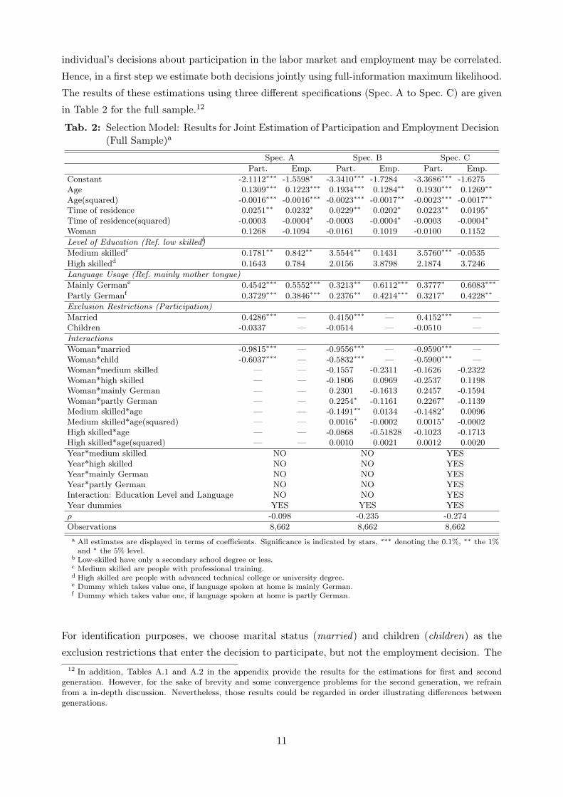
individual’s decisions about participation in the labor market and employment may be correlated.

Hence, in a first step we estimate both decisions jointly using full-information maximum likelihood.

The results of these estimations using three different specifications (Spec. A to Spec. C) are given

in Table 2 for the full sample.12

Tab. 2: Selection Model: Results for Joint Estimation of Participation and Employment Decision(Full Sample)a

Spec. A Spec. B Spec. C

Part. Emp. Part. Emp. Part. Emp.

Constant -2.1112∗∗∗ -1.5598∗ -3.3410∗∗∗ -1.7284 -3.3686∗∗∗ -1.6275Age 0.1309∗∗∗ 0.1223∗∗∗ 0.1934∗∗∗ 0.1284∗∗ 0.1930∗∗∗ 0.1269∗∗

Age(squared) -0.0016∗∗∗ -0.0016∗∗∗ -0.0023∗∗∗ -0.0017∗∗ -0.0023∗∗∗ -0.0017∗∗

Time of residence 0.0251∗∗ 0.0232∗ 0.0229∗∗ 0.0202∗ 0.0223∗∗ 0.0195∗

Time of residence(squared) -0.0003 -0.0004∗ -0.0003 -0.0004∗ -0.0003 -0.0004∗

Woman 0.1268 -0.1094 -0.0161 0.1019 -0.0100 0.1152

Level of Education (Ref. low skilledb)

Medium skilledc 0.1781∗∗ 0.842∗∗ 3.5544∗∗ 0.1431 3.5760∗∗∗ -0.0535

High skilledd 0.1643 0.784 2.0156 3.8798 2.1874 3.7246

Language Usage (Ref. mainly mother tongue)

Mainly Germane 0.4542∗∗∗ 0.5552∗∗∗ 0.3213∗∗ 0.6112∗∗∗ 0.3777∗ 0.6083∗∗∗

Partly Germanf 0.3729∗∗∗ 0.3846∗∗∗ 0.2376∗∗ 0.4214∗∗∗ 0.3217∗ 0.4228∗∗

Exclusion Restrictions (Participation)

Married 0.4286∗∗∗ — 0.4150∗∗∗ — 0.4152∗∗∗ —Children -0.0337 — -0.0514 — -0.0510 —

Interactions

Woman*married -0.9815∗∗∗ — -0.9556∗∗∗ — -0.9590∗∗∗ —Woman*child -0.6037∗∗∗ — -0.5832∗∗∗ — -0.5900∗∗∗ —Woman*medium skilled — — -0.1557 -0.2311 -0.1626 -0.2322Woman*high skilled — — -0.1806 0.0969 -0.2537 0.1198Woman*mainly German — — 0.2301 -0.1613 0.2457 -0.1594Woman*partly German — — 0.2254∗ -0.1161 0.2267∗ -0.1139Medium skilled*age — — -0.1491∗∗ 0.0134 -0.1482∗ 0.0096Medium skilled*age(squared) — — 0.0016∗ -0.0002 0.0015∗ -0.0002High skilled*age — — -0.0868 -0.51828 -0.1023 -0.1713High skilled*age(squared) — — 0.0010 0.0021 0.0012 0.0020

Year*medium skilled NO NO YESYear*high skilled NO NO YESYear*mainly German NO NO YESYear*partly German NO NO YESInteraction: Education Level and Language NO NO YESYear dummies YES YES YES

ρ -0.098 -0.235 -0.274

Observations 8,662 8,662 8,662

a All estimates are displayed in terms of coefficients. Significance is indicated by stars, ∗∗∗ denoting the 0.1%, ∗∗ the 1%and ∗ the 5% level.

b Low-skilled have only a secondary school degree or less.c Medium skilled are people with professional training.d High skilled are people with advanced technical college or university degree.e Dummy which takes value one, if language spoken at home is mainly German.f Dummy which takes value one, if language spoken at home is partly German.

For identification purposes, we choose marital status (married) and children (children) as the

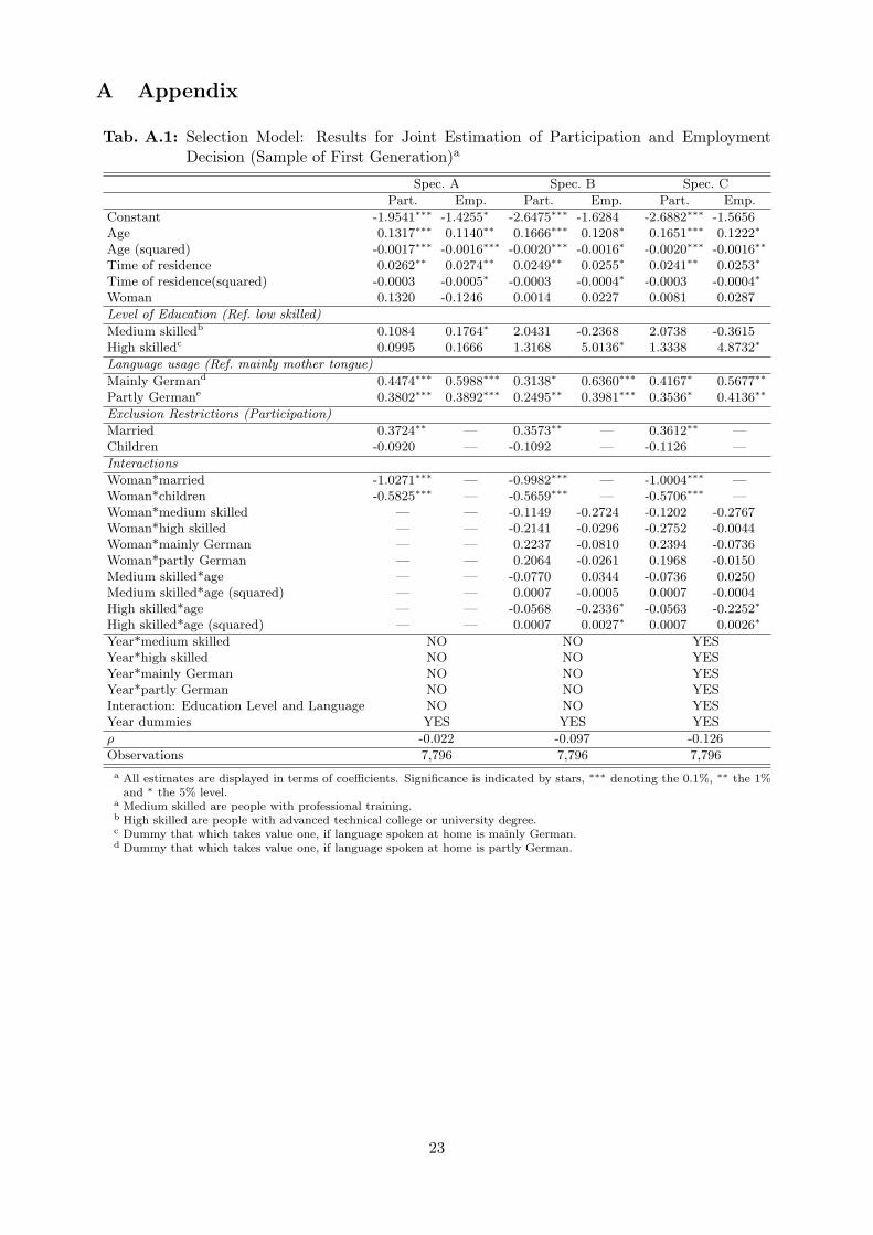
exclusion restrictions that enter the decision to participate, but not the employment decision. The12 In addition, Tables A.1 and A.2 in the appendix provide the results for the estimations for first and second

generation. However, for the sake of brevity and some convergence problems for the second generation, we refrainfrom a in-depth discussion. Nevertheless, those results could be regarded in order illustrating differences betweengenerations.

11

variables of language usage are regarded in both equations. Effects are estimated for dummies for

speaking mainly and speaking partly German at home with speaking mother tongue as a reference

group. Moreover, to improve explanatory power, some socio-economic variables are added to

the models. In particular, person’s age and time of residence (i.e. the years the individual lives

in Germany) as well as the squares are considered in both equations. To take account of gender

differences, we incorporated a dummy for sex, taking value 1 for females (woman). As productivity

is closely related to qualification, we estimate the effect of medium- or high-qualification in reference

to low-qualification. Finally, year dummies for the waves are regarded in all three specifications

to capture macroeconomic and composition effects. Specifications B and C differ from the basic

specification in the number of interactions included. In B, we additionally take into account

interactions between skills and language usage with gender and age. C extends the model to

consider a number of interactions for the year dummies and language usage with education level.

However, including these interactions does not provide great advantage in terms of precision of the

estimates. For that reason, we rely on the more parsimonious specification B for the estimations

of the second-stage (earnings equation, see below).13

Particular interest should be devoted to the coefficient of correlation (ρ) in the joint model. In

all three specifications presented in Table 2, the estimate is insignificant. For that reason, both

decisions could be estimated separately using univariate probit models. The results of the separate

models are given in Table 3.14 The estimates of the language variables clearly point towards a pos-

itive relationship between usage of the host country’s language and both the decision to participate

in the labor market and the employment chances. Although coefficients in the Tables can not be

interpreted as marginal effects, it becomes obvious from the scale that speaking mainly German

has an even stronger effect than using it only partly. Taking a look at the variables used as the

exclusion restrictions indicates that marriage has a positive effect on participation whereas having

children is insignificant at first sight. However, taking into account interactions, particularly with

gender, there is an indication that married men are more likely to participate in the labor market

than the singles; however, for females the reverse is true. Moreover, having children reduces par-

ticipation of foreign women as well. These findings may pinpoint to traditional attitudes of the

foreign population in Germany. Men are the primary earners, while women carry out household

duties and child care with financial support of their spouses15.

With respect to the other variables, most findings are in line with the expectations. Results

establish positive, but concave relationships between individual’s age and time of residence and

participation and employment. With respect to the level of education, medium-skilled people

experience a higher propensity to participate than the low-skilled. Maybe due to the small number13 In order to obtain the “best” specification, we carried out a quite extensive testing of different specifications.

Decisions were made using tests of (joint) significance for single variables, groups of variables and the whole set.14 In addition, the estimation results for first and second generation are given in Tables A.1 and A.2 for joint

estimation and Tables A.3 and A.4 for separate estimation in the appendix.15 Simple descriptive evidence supports this view: female participation rates of foreigners are 58 vs. 75 percent of

the native Germans; and the average number of children per household is 1.30 for foreigners and 0.91 for the nativeGermans.

12

Tab. 3: Selection Model: Results for Separate Estimation of Participation and EmploymentDecision (Full Sample)a



Constant -2.1084∗∗∗ -1.6787∗∗∗ -3.3003∗∗∗ -2.1721∗∗∗ -3.3173∗∗∗ -2.1457∗

Age 0.1309∗∗∗ 0.1260∗∗∗ 0.1915∗∗∗ 0.1460∗∗∗ 0.1906∗∗∗ 0.1473∗∗∗

Age(squared) -0.0016∗∗∗ -0.0017∗∗∗ -0.0023∗∗∗ -0.0019∗∗∗ -0.0023∗∗∗ -0.0019∗∗∗

Time of residence 0.0251∗∗∗ 0.0239∗∗∗ 0.0231∗∗∗ 0.0222∗∗ 0.0225∗∗ 0.0218∗

Time of residence(squared) -0.0003∗∗ -0.0004∗∗ -0.0003∗ -0.0004∗∗ -0.0003 -0.0004∗

Woman 0.1225 -0.1498∗∗∗ -0.0211 -0.0416 -0.0156 -0.0508

Level of Education (Ref. low skilled)

Medium skilledb 0.1793∗∗∗ 0.1930∗∗∗ 3.4741∗∗∗ 0.5311 3.4787∗∗∗ 0.4039High skilledc 0.1646∗∗ 0.1863∗ 1.8790 4.1846∗ 2.0217 4.0926∗


Mainly Germand 0.4547∗∗∗ 0.5767∗∗∗ 0.3220∗∗∗ 0.6288∗∗∗ 0.3789∗ 0.6357∗∗∗

Partly Germane 0.3734∗∗∗ 0.4012∗∗∗ 0.2375∗∗∗ 0.4377∗∗∗ 0.3798∗ 0.4500∗∗


Married 0.4239∗∗∗ — 0.4041∗∗∗ — 0.4025∗∗∗ —Children -0.0335 — -0.0506 — -0.0497 —

Interactions

Woman*married -0.9776∗∗∗ — -0.9478∗∗∗ — -0.9503∗∗∗ —Woman*children -0.6024∗∗∗ — -0.5828∗∗∗ — -0.5903∗∗∗ —Woman*medium skilled — — -0.1591∗ -0.2282∗ -0.1675 -0.2288Woman*high skilled — — -0.1816 0.0954 -0.2490 0.1158Woman*mainly German — — 0.2298∗ -0.0805 0.2451 -0.0644Woman*partly German — — 0.2260∗∗ -0.0610 0.2283∗ -0.0496Medium skilled*age — — -0.1447∗∗∗ -0.0038 -0.1429∗ -0.0104Medium skilled*age (squared) — — 0.0015∗∗ -0.0001 0.0015∗ 0.0000High skilled*age — — -0.0797 -0.1969∗ -0.0931 -0.1885High skilled*age(squared) — — 0.0009 0.0023∗ 0.0010 0.0022

Year*medium skilled NO NO NO NO YES YESYear*high skilled NO NO NO NO YES YESYear*mainly German NO NO NO NO YES YESYear*partly German NO NO NO NO YES YESInteraction: Education Level and Language NO NO NO NO YES YESYear dummies YES YES YES YES YES YES

Observations 8,662 6,477 8,662 6,477 8,662 6,477

adj. R2 0.2133 0.0558 0.2199 0.0596 0.2240 0.0652


b Medium skilled are people with professional training.c High skilled are people with advanced technical college or university degree.d Dummy that takes value one, if language spoken at home is mainly German.e Dummy that takes value one, if language spoken at home is partly German.

of foreigners who are high-skilled, estimations do not provide evidence that those differ in their

behavior from the low-skilled in terms of participation. In contrast, high-skilled have a significant

higher probability with respect to employment.

5.2 The Impact of Language Usage on Earnings

Given the results from the joint estimation of the selection model, there is no need to assume

a joint dependence of foreigners’ earnings on the participation and the employment decisions.

Nevertheless, neglecting self-selection at all in the earnings equation could lead to biased estimates

bearing in mind the explanatory power of the separate models. To consider self-selection in terms

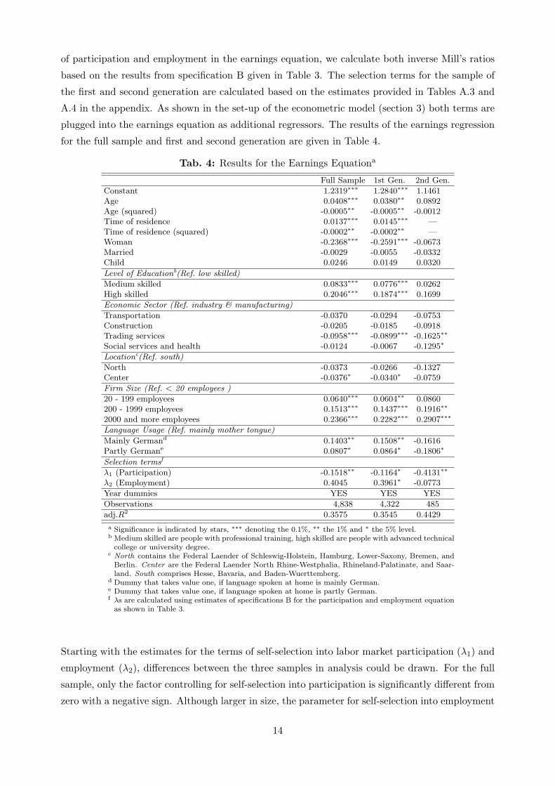
13

of participation and employment in the earnings equation, we calculate both inverse Mill’s ratios

based on the results from specification B given in Table 3. The selection terms for the sample of

the first and second generation are calculated based on the estimates provided in Tables A.3 and

A.4 in the appendix. As shown in the set-up of the econometric model (section 3) both terms are

plugged into the earnings equation as additional regressors. The results of the earnings regression

for the full sample and first and second generation are given in Table 4.

Tab. 4: Results for the Earnings Equationa

Full Sample 1st Gen. 2nd Gen.

Constant 1.2319∗∗∗ 1.2840∗∗∗ 1.1461Age 0.0408∗∗∗ 0.0380∗∗ 0.0892Age (squared) -0.0005∗∗ -0.0005∗∗ -0.0012Time of residence 0.0137∗∗∗ 0.0145∗∗∗ —Time of residence (squared) -0.0002∗∗ -0.0002∗∗ —Woman -0.2368∗∗∗ -0.2591∗∗∗ -0.0673Married -0.0029 -0.0055 -0.0332Child 0.0246 0.0149 0.0320

Level of Educationb(Ref. low skilled)

Medium skilled 0.0833∗∗∗ 0.0776∗∗∗ 0.0262High skilled 0.2046∗∗∗ 0.1874∗∗∗ 0.1699

Economic Sector (Ref. industry & manufacturing)

Transportation -0.0370 -0.0294 -0.0753Construction -0.0205 -0.0185 -0.0918Trading services -0.0958∗∗∗ -0.0899∗∗∗ -0.1625∗∗

Social services and health -0.0124 -0.0067 -0.1295∗

Locationc(Ref. south)

North -0.0373 -0.0266 -0.1327Center -0.0376∗ -0.0340∗ -0.0759

Firm Size (Ref. < 20 employees )

20 - 199 employees 0.0640∗∗∗ 0.0604∗∗ 0.0860200 - 1999 employees 0.1513∗∗∗ 0.1437∗∗∗ 0.1916∗∗

2000 and more employees 0.2366∗∗∗ 0.2282∗∗∗ 0.2907∗∗∗


Mainly Germand 0.1403∗∗ 0.1508∗∗ -0.1616Partly Germane 0.0807∗ 0.0864∗ -0.1806∗

Selection termsf

λ1 (Participation) -0.1518∗∗ -0.1164∗ -0.4131∗∗

λ2 (Employment) 0.4045 0.3961∗ -0.0773

Year dummies YES YES YES

Observations 4,838 4,322 485

adj.R2 0.3575 0.3545 0.4429

a Significance is indicated by stars, ∗∗∗ denoting the 0.1%, ∗∗ the 1% and ∗ the 5% level.b Medium skilled are people with professional training, high skilled are people with advanced technical

college or university degree.c North contains the Federal Laender of Schleswig-Holstein, Hamburg, Lower-Saxony, Bremen, and

Berlin. Center are the Federal Laender North Rhine-Westphalia, Rhineland-Palatinate, and Saar-land. South comprises Hesse, Bavaria, and Baden-Wuerttemberg.

d Dummy that takes value one, if language spoken at home is mainly German.e Dummy that takes value one, if language spoken at home is partly German.f λs are calculated using estimates of specifications B for the participation and employment equation

as shown in Table 3.

Starting with the estimates for the terms of self-selection into labor market participation (λ1) and

employment (λ2), differences between the three samples in analysis could be drawn. For the full

sample, only the factor controlling for self-selection into participation is significantly different from

zero with a negative sign. Although larger in size, the parameter for self-selection into employment

14

is of no statistical significance. In contrast, the estimates for the more homogeneous first generation

sample are more pronounced. Here, both terms have significant influence on foreigners’ earnings.

The estimates show that being more familiar with host’s countries language lead to higher earnings.

Speaking mainly German, for example, lead on average to 14.03 percent (full sample) higher

earnings than speaking mainly mother tongue at home. Even using German partly at home

coincides with an earnings’ increase of about 8.07 percent compared to the reference group. These

differences are even stronger for the first generation. Here, those who speak mainly German

earn on average about 15.08 percent more than people using their home country’s language in the

household. Also when using German language only partly at home, earnings are about 8.64 percent

higher. The estimates for the second generation are somewhat contra-intuitive. Speaking mainly

German has no significant effect while speaking partly German results in lower earnings than

speaking the language of the country of citizenship. However, given the clearly smaller number of

observations the estimates should not be overrated.

The results presented are comparable with other studies. Dustmann (1994) finds a 15.3 percent

wage increase for females and a 7.3 percent increase for males who report to have good or very good

writing abilities in German language. Chiswick and Miller (1999) report higher wages by about

8 percent for migrant males and 17 percent for females who are proficient in both speaking and

reading English using the 1989 Legalized Population Survey (LPS) for the United States. For Great

Britain Shields and Price (2002) establish that language fluency increases the mean occupational

wage by about 16.5 percent. Chiswick, Lee, and Miller (2005) find out that immigrants who are

proficient in English have 19 percent higher earnings than those with limited English language

skills using the Longitudinal Survey of Immigrants to Australia 1993-1995. For Israel Berman,

Lang, and Siniver (2000) predict a 23 percent earnings’ increase for immigrants from the former

Soviet Union who fluently speak Hebrew in 1994.

The parameters of the other variables incorporated in the model show that earnings increase with

age by about 4 percent; each additional year of living in Germany raises earnings by additional

1.45 percent for the first generation (1.37 percent for the full sample). The gender wage gap is

particularly strong within the first generation. Here, men earn about 25.91 percent more than

women. For the second generation, no significant difference could be determined. The benefits

from better education are larger in the full sample than in the sample of the first generation.

Medium-skilled, i.e. people having completed a professional training, earn about 8.33 (7.76 first

generation) percent more than low-skilled; high-skilled, i.e. those having an advanced technical

college (Fachhochschule) or university degree, earn even 20.46 (18.74) percent more. The reason

for the smaller earnings differences in the first generation may be due to the composition of this

group. As mentioned before, first generation immigrants were recruited as unskilled or low-skilled

labor to reduce labor supply shortages in West Germany during the 1960s and early 1970s. As

this group has been employed for a long time, people’s human capital was appreciated over the

years without formal attestation; consequently, wages increased over the years to levels above that

of the average unskilled or low-skilled worker. Choice of the economic sector seems to be relatively

15

ineffective with respect to earnings except when foreigners work in the trading sector. Compared

to working in industry and manufacturing this leads to about 9 to 9.5 percent lower earnings. The

firm size plays a more important role in wage setting as the results reveal bigger firms paying higher

wages with about 25 percent wage differential between the large (more than 2000 employees) and

small (less than 20) firms. Concerning the geographical location, the results show that earnings in

central regions are somewhat smaller (by about 3.7%) compared to the south.

Apart from the minor problems for the second generation, we could recapitulate the (intermediate)

findings as follows: the results for the full sample and the sample of the first generation clearly

indicate that speaking German is important for foreigners not only for the decision whether to

supply labor or becoming employed, but for the resulting earnings, too. Hence, improving the

command of German language for foreigners is important in order to increase earnings and, there-

fore, social security contributions and taxes. Moreover, as the results from the selection models

indicate, particularly women speaking their native languages at home refrain from participating

in the labor market. Improving the command of German language for this group may provide a

further potential of productivity to the economy.

5.3 Considering Self-Selection into Economic Sector and Occupation

Theory predicts that workers with higher productivity enter higher paid jobs. Therefore, even

though controlling for self-selection into participation and employment, earnings may be affected

by worker’s choice for type of occupation and economic sector. Therefore, we extend our model to

explicitly control for selection through these channels. Using the sub-sample of employed, we take

account of self-selection in the economic sector modeled as the probability of working in a basic or

high-tech industry and of self-selection in occupation choice modeled as the probability of being

a qualified/highly-qualified white-collar worker. Analogously to our empirical model discussed in

section 3, both choices are considered as joint decisions in a first step. Assuming joint normality

of the errors, estimation is carried out using a bivariate probit model.

In the extended model, the selection terms for participation (λ1) and employment (λ2) estimated in

the first stage are considered as auxiliary variables in the bivariate probit. The extended earnings

equation (Eq. 6), is augmented by the two auxiliary selectivity variables capturing economic sector

choice (λ3) and type of occupation (λ4):

E(w|X) = Xβ + λ1σu1 + λ2σu2 + λ3σu3 + λ4σu4. (7)

The additional parameters λ3 and λ4 are calculated analogously to the λ1 and λ2 using the esti-

mates of the type of occupation and economic sector choice equations.

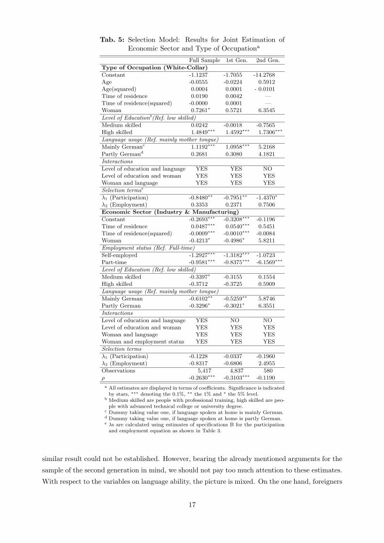
The results of the bivariate probit model on type of occupation and economic sector choice are

given in Table 5 distinguishing full sample and first and second generation. The estimate for the

correlation coefficient (ρ) is highly significant for the full sample and the first generation; hence,

both choices have to be estimated jointly to avoid selection bias. For the second generation, a

16

Tab. 5: Selection Model: Results for Joint Estimation ofEconomic Sector and Type of Occupationa

Full Sample 1st Gen. 2nd Gen.

Type of Occupation (White-Collar)

Constant -1.1237 -1.7055 -14.2768Age -0.0555 -0.0224 0.5912Age(squared) 0.0004 0.0001 - 0.0101Time of residence 0.0190 0.0042 —Time of residence(squared) -0.0000 0.0001 —Woman 0.7261∗ 0.5721 6.3545


Medium skilled 0.0242 -0.0018 -0.7565High skilled 1.4849∗∗∗ 1.4592∗∗∗ 1.7306∗∗∗

Language usage (Ref. mainly mother tongue)

Mainly Germanc 1.1192∗∗∗ 1.0958∗∗∗ 5.2168

Partly Germand 0.2681 0.3080 4.1821

Interactions

Level of education and language YES YES NOLevel of education and woman YES YES YESWoman and language YES YES YES

Selection termse

λ1 (Participation) -0.8480∗∗ -0.7951∗∗ -1.4370∗

λ2 (Employment) 0.3353 0.2371 0.7506

Economic Sector (Industry & Manufacturing)

Constant -0.2693∗∗∗ -0.3208∗∗∗ -0.1196Time of residence 0.0487∗∗∗ 0.0540∗∗∗ 0.5451Time of residence(squared) -0.0009∗∗∗ -0.0010∗∗∗ -0.0084Woman -0.4213∗ -0.4986∗ 5.8211

Employment status (Ref. Full-time)

Self-employed -1.2927∗∗∗ -1.3182∗∗∗ -1.0723Part-time -0.9581∗∗∗ -0.8375∗∗∗ -6.1569∗∗∗


Medium skilled -0.3397∗ -0.3155 0.1554High skilled -0.3712 -0.3725 0.5909


Mainly German -0.6102∗∗ -0.5259∗∗ 5.8746Partly German -0.3296∗ -0.3021∗ 6.3551

Interactions

Level of education and language YES NO NOLevel of education and woman YES YES YESWoman and language YES YES YESWoman and employment status YES YES YES

Selection terms

λ1 (Participation) -0.1228 -0.0337 -0.1960λ2 (Employment) -0.8317 -0.6806 2.4955

Observations 5,417 4,837 580ρ -0.2630∗∗∗ -0.3103∗∗∗ -0.1190

a All estimates are displayed in terms of coefficients. Significance is indicatedby stars, ∗∗∗ denoting the 0.1%, ∗∗ the 1% and ∗ the 5% level.

b Medium skilled are people with professional training, high skilled are peo-ple with advanced technical college or university degree.

c Dummy taking value one, if language spoken at home is mainly German.d Dummy taking value one, if language spoken at home is partly German.e λs are calculated using estimates of specifications B for the participation

and employment equation as shown in Table 3.

similar result could not be established. However, bearing the already mentioned arguments for the

sample of the second generation in mind, we should not pay too much attention to these estimates.

With respect to the variables on language ability, the picture is mixed. On the one hand, foreigners

17

speaking mainly German at home have a clearly higher probability to be white-collar workers, on

the other hand, they have lower chances of working in industry and manufacturing (in general

highly paid industries). For the latter choice, even speaking German at home partly reduces

the probability compared to speaking only mother tongue. Becoming a white-collar worker is

more probable for high-skilled individuals. Interestingly, women are more likely to fill white-collar

positions than men. In addition, people with a medium education level in Germany are less likely

than the low-skilled to work in industry and manufacturing.

With these estimates at hand we calculate two further auxiliary terms capturing selection into

economic sector (λ3) and type of occupation (λ4) non-linearly and augment the earnings equation

as stated above. Table 6 provides the corresponding results. To check the sensitivity of the

estimates, along with the results for the full specification a more parsimonious model (without

taking into account employment status and several interactions) and a model without additional

selection terms are presented. In the parsimonious model, neither the coefficients for the language

terms nor that of the selection into industry and occupation terms are significant. However,

the dummy variables for language and selection into industry and occupation terms are jointly

significant; hence, we cannot drop all four of them from the model. It should be noted that

dropping the language variables leads to significant estimates for the selection into industry and

occupation terms. On the other hand, disregarding selection into industry and occupation gives

language dummies statistical significance. These results make it difficult to say whether language

ability affects earnings directly or indirectly, which is in contrast to the basic model (see Table

4) indicating a direct effect. However, it is in line with the theoretical considerations laid out in

section 2. If we have non-discriminating firms, no wage premium due to language usage could

be expected. This implies that language affects the choice of occupation and economic sector as

well as, more fundamentally, decisions about participation and employment but not wages per se.

Hence, the significant effect of language in Table 4 is likely to be an indirect effect of language

usage on earnings through occupation and economic sector choice.

18

Tab. 6: Earnings Equation with Selection into Type ofOccupation and Economic Sectora

Full Spec. Pars. Spec. w/o selec.

Constant 1.3070∗ 1.2503∗∗∗ 1.2464∗∗∗

Age 0.0364 0.0402∗∗∗ 0.0380∗∗

Age(squared) -0.0004 -0.0005∗∗ -0.0005∗∗

Time of residence 0.0178∗∗∗ 0.0143∗∗∗ 0.0139∗∗∗

Time of residence(squared) -0.0003∗∗ -0.0002∗∗ -0.0002∗∗

Women -0.2688∗∗∗ -0.2419∗∗∗ -0.2320∗∗∗

Married 0.0085 -0.0031 0.0000Children 0.0256 0.0259 0.0317


Medium skilled -0.3604 0.0790∗∗ 0.0803∗∗∗

High skilled 0.4028 0.1926∗∗ 0.2092∗∗∗


Mainly Germanc 0.1071 0.1286 0.1211∗∗

Partly Germand 0.0848 0.0766 0.0732∗

Employment status (Ref. Full-time)

Self-employed 0.0916 — —Part-time -0.2920∗∗ — —

Sector (Ref. industry & manufacturing)

Transportation -0.0396 -0.0389 —Construction -0.0151 -0.0204 —Trading services -0.0940∗∗∗ -0.0983∗∗∗ —Social services and health -0.0041 -0.0150 —

Firm size (Ref. < 20 employees )

20 - 199 employees 0.0865∗∗∗ 0.0681∗∗∗ 0.0799∗∗∗

200 - 1999 employees 0.1696∗∗∗ 0.1558∗∗∗ 0.1823∗∗∗

2000 and more employees 0.2566∗∗∗ 0.2408∗∗∗ 0.2615∗∗∗

Locatione(Ref. south )

North -0.0373 -0.0385 -0.0500Center -0.0336∗ -0.0379∗ -0.0416∗∗

Interactions

Skill Level and age YES NO NOSkill Level and woman YES NO NOEmployment status and woman YES NO NO

Selection termsf

λ1 (Participation) -0.1367∗ -0.1624∗∗ -0.1727∗∗∗

λ2 (Employment) 0.4313 0.3840 0.3523λ3 (Economic sector) -0.0919 -0.0169 —λ4 (Occupation type) 0.1133∗ 0.0219 —

Year dummies YES YES YES


a Significance is indicated by stars, ∗∗∗ denoting the 0.1%, ∗∗ the 1% and∗ the 5% level.

b Medium skilled are people with professional training, high skilled arepeople with advanced technical college or university degree.

c Dummy taking value one, if language spoken at home is mainly German.d Dummy taking value one, if language spoken at home is partly German.e North contains the Federal Laender of Schleswig-Holstein, Hamburg,

Lower-Saxony, Bremen, and Berlin. Center are the Federal LaenderNorth Rhine-Westphalia, Rhineland-Palatinate, and Saarland. Southcomprises Hesse, Bavaria, and Baden-Wuerttemberg.

f λ1 and λ2 are calculated using estimates of specifications B for theparticipation and employment equation as shown in Table 3. λ3 andλ4 are calculated using estimates for the economic sector and type ofoccupation equation as shown in Table 5.

19

6 Conclusion

There is a quite comprehensive international evidence showing that foreigners speaking the lan-

guage of the host country well are better off in terms of earnings than those with only a poor

command. However, issues of self-selection are often neglected and, thereby, effects of language

on earnings may be overestimated. Moreover, estimates may suffer from inaccurate measures of

language ability based on self-assessed survey information. In this study, the effects of language

ability on earnings are analyzed for foreigners in Germany taking account of various dimensions

of selection, i.e. labor market participation, employment, choice of economic sector and type of

occupation. Problems of the language ability measure are mitigated by using the more easily (and

therefore more accurately) self-reported information on language usage in the household.

Based upon theoretical considerations that assume that no wage premium due to language could

be expected in a world of non-discriminating firms, we provide empirical evidence based on data

from GSOEP. Starting with a basic model that takes account of two channels of self-selection

regarding labor market participation and employment, the effects of language ability on earnings

are estimated. The results show that language ability is a relevant determinant both for labor

market participation and employment as well. In addition, foreigners who speak mainly German in

the household receive on average about 14 percent higher wages compared to those using the native

language at home. Hence, the results clarify that language ability is an important and valuable

asset not only for integration, but also for prosperity. In a second step, we extend the model to

capture selection patterns into economic sector and type of occupation as theory predicts high

productive workers to fill high-paid positions. Again, for both decisions language ability is crucial,

although the picture is reverted. Whereas using German in the household as the main language

increases the probability for foreigners to be high-qualified white-collar workers, this reduces the

probability for working in industry and manufacturing. When the earnings equation is augmented

with two additional variables to control for these selection patterns, no direct effects of language

ability on earnings can be established anymore. Hence, language ability only indirectly affects

foreigners’ earnings in Germany, but is a major determinant of the various selection processes.

The analysis distinguishing first and second generation provides only a first approach and shows

that second generation immigrants use German more frequently in the household. Unfortunately,

no clear effects for this groups could be found. Hence, further research on the effects of language

ability on earnings for the second generation migrants is needed. However, for that purpose more

detailed and comprehensive information than that provided in GSOEP is required. The main

finding of the paper clearly indicates that improving the command of the German language for

foreigners should be a major item on the public agenda in order to increase labor market and

economic integration of this group. In this context, a particular focus should be given to foreign

women speaking only native languages at home. Although the government offers language courses,

the use and usefulness of these measures should be evaluated thoroughly.

20

References

Aldashev, A., J. Gernandt, and S. L. Thomsen (2007): “Earnings Prospects for People with

Migration Background in Germany,” Discussion Paper No. 07-31, ZEW.

Berman, E., K. Lang, and E. Siniver (2000): “Language-Skill Complementarity: Returns to

Immigrant Language Acquisition,” Working Paper 7737, NBER.

Burdett, K., and D. Mortensen (1998): “Wage Differentials, Employer Size and Unemploy-

ment,” International Economic Review, 39, 257–273.

Chiswick, B. R. (1978): “The Effect of Americanization on the Earnings of Foreign-born Men,”

Journal of Political Economy, 86(5), 897–921.

(1991): “Speaking, Reading, and Earnings among Low-skilled Immigrants,” Journal of

Labor Economics, 9(2), 149–170.

Chiswick, B. R., Y. L. Lee, and P. W. Miller (2005): “Immigrant Earnings: A Longitudinal

Analysis,” Review of Income and Wealth, 51(4), 485–503.

Chiswick, B. R., and P. W. Miller (1995): “The Endogeneity between Language and Earnings:

International Analyses,” Journal of Labor Economics, 13(2), 246–288.

(1999): “Language Skills and Earnings Among Legalized Aliens,” Journal of Population

Economics, 12, 63–89.

Dustmann, C. (1994): “Speaking Fluency, Writing Fluency and Earnings of Migrants,” Journal

of Population Economics, 7, 133–156.

Dustmann, C., and A. van Soest (2001): “Language Fluency and Earnings: Estimation with

Misclassified Language Indicators,” The Review of Economic and Statistics, 83(4), 663–674.

(2002): “Language and the Earnings of Immigrants,” Industrial and Labor Relations

Review, 55(3), 473–492.

Haisken-DeNew, J., and J. Frick (2005): “Desktop Companion of the German Socio-Economic

Panel,” Discussion paper, DIW, Berlin.

Heckman, J. (1976): “The Common Structure of Statistical Models of Truncation, Sample Se-

lection, and Limited Dependent Variables and a Simple Estimator for Such Models,” Annals of

Economic and Social Measurement, 5, 475–492.

(1979): “Sample Selection Bias as a Specification Error,” Econometrica, 47(1), 153–161.

Lee, L. F. (1976): “Estimation of Limited Dependent Variables by Two-Stage Methods,” Unpub-

lished Ph.D. Dissertation, University of Rochester.

21

Maddala, G. (1983): Limited-dependent and Qualitative Variables in Econometrics. Cambridge

University Press.

Manning, A. (2003): Monopsony in Motion. Princeton University Press.

McManus, W., W. Gould, and F. Welch (1983): “Earnings of Hispanic Men: The Role of

English Language Proficiency,” Journal of Labor Economics, 1(2), 101–130.

Mohanty, M. (2001): “Determination of Participation Decision, Hiring Decision, and Wages

in a Double Selection Framework: Male-Female Wage Differentials in the U.S. Labor Market

Revisited,” Contemporary Economic Policy, 19(2), 197–212.

Mortensen, D. T. (2003): Wage Dispersion: Why Are Similar Workers Paid Differently? Cam-

bridge, Massachusetts.

Riphahn, R. (2003): “Cohort Effects in the Educational Attainment of Second Generation Im-

migrants in Germany: An Analysis of Census Data,” Journal of Population Economics, 16(4),

711–737.

(2005): “Are there Diverging Time Trends in the Educational Attainment of Nationals

and Second Generation Immigrants?,” Jahrbucher fur Nationalokonomie und Statistik, 225(3),

325–346.

Shields, M. A., and S. W. Price (2002): “The English Language Fluency and Occupational

Success of Ethnic Minority Immigrant Men Living in English Metropolitan Areas,” Journal of

Population Economics, 15, 137–160.

22

A Appendix

Tab. A.1: Selection Model: Results for Joint Estimation of Participation and EmploymentDecision (Sample of First Generation)a



Constant -1.9541∗∗∗ -1.4255∗ -2.6475∗∗∗ -1.6284 -2.6882∗∗∗ -1.5656Age 0.1317∗∗∗ 0.1140∗∗ 0.1666∗∗∗ 0.1208∗ 0.1651∗∗∗ 0.1222∗

Age (squared) -0.0017∗∗∗ -0.0016∗∗∗ -0.0020∗∗∗ -0.0016∗ -0.0020∗∗∗ -0.0016∗∗

Time of residence 0.0262∗∗ 0.0274∗∗ 0.0249∗∗ 0.0255∗ 0.0241∗∗ 0.0253∗

Time of residence(squared) -0.0003 -0.0005∗ -0.0003 -0.0004∗ -0.0003 -0.0004∗

Woman 0.1320 -0.1246 0.0014 0.0227 0.0081 0.0287


Medium skilledb 0.1084 0.1764∗ 2.0431 -0.2368 2.0738 -0.3615High skilledc 0.0995 0.1666 1.3168 5.0136∗ 1.3338 4.8732∗


Mainly Germand 0.4474∗∗∗ 0.5988∗∗∗ 0.3138∗ 0.6360∗∗∗ 0.4167∗ 0.5677∗∗

Partly Germane 0.3802∗∗∗ 0.3892∗∗∗ 0.2495∗∗ 0.3981∗∗∗ 0.3536∗ 0.4136∗∗


Married 0.3724∗∗ — 0.3573∗∗ — 0.3612∗∗ —Children -0.0920 — -0.1092 — -0.1126 —

Interactions

Woman*married -1.0271∗∗∗ — -0.9982∗∗∗ — -1.0004∗∗∗ —Woman*children -0.5825∗∗∗ — -0.5659∗∗∗ — -0.5706∗∗∗ —Woman*medium skilled — — -0.1149 -0.2724 -0.1202 -0.2767Woman*high skilled — — -0.2141 -0.0296 -0.2752 -0.0044Woman*mainly German — — 0.2237 -0.0810 0.2394 -0.0736Woman*partly German — — 0.2064 -0.0261 0.1968 -0.0150Medium skilled*age — — -0.0770 0.0344 -0.0736 0.0250Medium skilled*age (squared) — — 0.0007 -0.0005 0.0007 -0.0004High skilled*age — — -0.0568 -0.2336∗ -0.0563 -0.2252∗

High skilled*age (squared) — — 0.0007 0.0027∗ 0.0007 0.0026∗

Year*medium skilled NO NO YESYear*high skilled NO NO YESYear*mainly German NO NO YESYear*partly German NO NO YESInteraction: Education Level and Language NO NO YESYear dummies YES YES YES

ρ -0.022 -0.097 -0.126



a Medium skilled are people with professional training.b High skilled are people with advanced technical college or university degree.c Dummy that which takes value one, if language spoken at home is mainly German.d Dummy that which takes value one, if language spoken at home is partly German.

23

Tab. A.2: Selection Model: Results for Joint Estimation of Participation and EmploymentDecision (Sample of Second Generation)a,b



Constant 1.0882 1.2909 5.7881 5.5187 5.2462 6.7316Age -0.0775 -0.0206 -0.4563 -0.3303 -0.3774 -0.4166Age (squared) 0.0014 0.0005 0.0089 0.0054 0.0077 0.0066Time of residence — — — — — —Time of residence(squared) — — — — — —Woman 0.0283 -0.1118 0.0207 0.8267 0.1468 -0.1875


Medium skilledc 0.7228∗∗∗ 0.2162 1.5627 -3.9363 3.1832 0.8565

High skilledd 0.9055∗∗∗ 0.3141 -13.0034 -16.5763 — —


Mainly Germane 0.5054∗ 0.2043 0.5060 0.7074 -0.1096 1.1818

Partly Germanf 0.3896∗ 0.2247 0.3605 0.9096∗ -0.1555 0.6739


Married 0.6536∗∗ — 0.6900∗∗ — 0.7423∗∗ —Children 0.0780 — 0.0249 — 0.0964 —

Interactions

Woman*married -0.9077∗∗ — -0.9358∗∗ — -0.9386∗∗ —Woman*child -0.5309 — -0.4750 — -0.5616 —Woman*medium skilled — — -0.4434 0.0675 -0.6301 0.0500Woman*high skilled — — 0.4314 5.8398∗∗∗ 0.4241 5.0660Woman*mainly German — — 0.0795 -1.0368∗ 0.1404 0.0535Woman*partly German — — 0.1446 -1.3619∗∗ 0.0245 -0.3504Medium skilled*age — — 0.0875 0.2766 0.0017 0.2895Medium skilled*age(squared) — — -0.0037 -0.0045 -0.0024 -0.0045High skilled*age — — 0.8634 1.0139 0.3701 1.7516High skilled*age(squared) — — -0.0136 -0.0152 -0.0065 -0.0263

Year*medium skilled NO NO YESYear*high skilled NO NO YESYear*mainly German NO NO YESYear*partly German NO NO YESYear dummies YES YES YESInteraction: Education Level and Language NO NO YES

ρ -0.877∗ -0.996 -0.983

Observations 866 866 866

a Due to the small number of observations, convergence of specification B and C was not achieved and maximizationwas stopped after 100 iterations. The results presented in Spec. B and Spec. C do not refer to a global maximum.

b All estimates are displayed in terms of coefficients. Significance is indicated by stars, ∗∗∗ denoting the 0.1%, ∗∗ the1% and ∗ the 5% level.

c Medium skilled are people with professional training.d High skilled are people with advanced technical college or university degree.e Dummy that which takes value one, if language spoken at home is mainly German.f Dummy that which takes value one, if language spoken at home is partly German.

24

Tab. A.3: Selection Model: Results for Separate Estimation of Participation and EmploymentDecision (Sample of First Generation)a

Model A Model B Model C


Constant -1.9533∗∗∗ -1.4524∗∗ -2.6310∗∗∗ -1.7893∗∗ -2.6668∗∗∗ -1.7745∗∗

Age 0.1316∗∗∗ 0.1149∗∗∗ 0.1658∗∗∗ 0.1269∗∗∗ 0.1640∗∗∗ 0.1300∗∗∗

Age (squared) -0.0017∗∗∗ -0.0016∗∗∗ -0.0020∗∗∗ -0.0017∗∗∗ -0.0020∗∗∗ -0.0017∗∗∗

Time of residence 0.0262∗∗∗ 0.0276∗∗∗ 0.0250∗∗∗ 0.0263∗∗∗ 0.0242∗∗∗ 0.0263∗∗∗

Time of residence (squared) -0.0003∗∗ -0.0005∗∗ -0.0003∗ -0.0005∗∗ -0.0003∗ -0.0005∗∗

Woman 0.1313 -0.1344∗∗ -0.0002 -0.0377 0.0066 -0.0488


Medium skilledb 0.1087∗∗ 0.1778∗∗∗ 2.0149∗ -0.1213 2.0365∗ -0.2117High skilledc 0.0997 0.1679∗ 1.2703 5.1115∗∗ 1.2772 5.0008∗∗


Mainly Germand 0.4475∗∗∗ 0.6037∗∗∗ 0.3145∗∗∗ 0.6433∗∗∗ 0.4194∗∗ 0.5808∗∗∗

Partly Germane 0.3803∗∗∗ 0.3929∗∗∗ 0.2498∗∗∗ 0.4048∗∗∗ 0.3538∗∗ 0.4272∗∗


Married 0.3714∗∗∗ — 0.3531∗∗∗ — 0.3482∗∗∗ —Child -0.0918 — -0.1080 — -0.1105 —

Interactions

Woman*married -1.0264∗∗∗ — -0.9956∗∗∗ — -0.9974∗∗∗ —Woman*child -0.5824∗∗∗ — -0.5659∗∗∗ — -0.5711∗∗∗ —Woman*medium skilled — — -0.1159 -0.2713∗∗ -0.1220 -0.2753∗∗

Woman*high skilled — — -0.2144 -0.0336 -0.2728∗ -0.0105Woman*mainly German — — 0.2232∗ -0.0480 0.2383∗ -0.0305Woman*partly German — — 0.2065∗ -0.0044 0.1971∗ 0.0125Medium skilled*age — — -0.0754 0.0295 -0.0715 0.0188Medium skilled*age (squared) — — 0.0007 -0.0005 0.0006 -0.0003High skilled*age — — -0.0543 -0.2381∗ -0.0531 -0.2310∗∗

High skilled*age (squared) — — 0.0007 0.0028∗ 0.0006 0.0028∗∗

Year*medium skilled NO NO NO NO YES YESYear*high skilled NO NO NO NO YES YESYear*mainly German NO NO NO NO YES YESYear*partly German NO NO NO NO YES YESInteraction: Education Level and Language NO NO NO NO YES YESYear dummies YES YES YES YES YES YES

Observations 7,796 5,793 7,796 5,793 7,796 5,793

adj. R2 0.2244 0.0600 0.2283 0.0643 0.2327 0.0701


b Medium skilled are people with professional training.c High skilled are people with advanced technical college or university degree.d Dummy that takes value one, if language spoken at home is mainly German.e Dummy that takes value one, if language spoken at home is partly German.

25

Tab. A.4: Selection Model: Results for Separate Estimation of Participation and EmploymentDecision (Sample of Second Generation)a,b

Model A Model B Model C


Constant 0.5759 0.4631 2.7705 2.2623 4.9796 4.9263

Age -0.0418 0.0012 -0.2429 -0.1532 -0.3427 -0.3034Age (squared) 0.0008 0.0001 0.0052 0.0028 0.0071 0.0050Woman -0.0296 -0.2881∗ -0.0257 0.5316 -0.0551 -0.8461

Level of Qualification (Ref. low skilled)

Medium skilleda 0.7069∗∗∗ 0.4172∗∗ 4.7501 0.2145 3.1106 6.0803

High skilledb 0.8657∗∗∗ 0.5021∗ -9.1897 -15.5554 — -19.6690


Mainly Germanc 0.5353∗ 0.5114 0.5114 0.9495∗ -0.2532 0.9667

Partly Germand 0.4243∗ 0.5236 0.3277 1.1328∗∗ -0.3516 0.3885


Married 0.5766∗∗ — 0.6271∗∗ — 0.6631∗∗ —Child 0.1027 — 0.0638 — 0.1148 —

Interactions

Woman*married -0.8006∗∗ — -0.8426∗∗∗ — -0.8743∗∗∗ —Woman*child -0.5107∗ — -0.4466 — -0.4696 —Woman*medium skilled — — -0.4611 0.1753 -0.6211∗∗ 0.1475Woman*high skilled — — 0.4278 — 0.4606 —Woman*mainly German — — 0.0701 -0.9717 0.2269 0.4747Woman*partly German — — 0.1611 -1.3443∗ 0.1721 0.0069Medium skilled*age — — -0.1369 0.0309 -0.0058 0.0305Medium skilled*age (squared) — — 0.0002 -0.0009 -0.0022 -0.0008High skilled*age — — 0.5993 0.9434 0.3703 1.5237High skilled*age(squared) — — -0.0091 -0.0140 -0.0064 -0.0228

Year*medium skilled NO NO NO NO YES YESYear*high skilled NO NO NO NO YES YESYear*mainly German NO NO NO NO YES YESYear*martly German NO NO NO NO YES YESInteraction: Education Level and Language NO NO NO NO YES YESYear dummies YES YES YES YES YES YES

Observations 866 684 866 650 823 642

adj.R2 0.1640 0.0576 0.1914 0.0789 0.2217 0.1500

a All estimates are displayed in terms of coefficients. Significance is indicated by stars, ∗∗∗ denoting the 0.1%, ∗∗ the1% and ∗ the 5% level.

b Time of residence equals age of individuals and is dropped from estimation.c Medium skilled are people with professional training.d High skilled are people with advanced technical college or university degree.e Dummy that which takes value one, if language spoken at home is mainly German.f Dummy that which takes value one, if language spoken at home is partly German.

26

Date post:	17-Aug-2019
Category:	Documents
Upload:	dangkhanh
View:	212 times
Download:	0 times

OTTO VON-GUERICKE-UNIVERSITY MAGDEBURG · 1 Introduction Earnings of foreigners have been...

Documents