Out-of-Distribution Generalization via Risk Extrapolation

Out-of-Distribution Generalization via Risk Extrapolation

David Krueger 1 2 Ethan Caballero 1 2 Joern-Henrik Jacobsen 3 4 Amy Zhang 1 5 6 Jonathan Binas 1 2

Dinghuai Zhang 1 2 Remi Le Priol 1 2 Aaron Courville 1 2

AbstractDistributional shift is one of the major obstacleswhen transferring machine learning predictionsystems from the lab to the real world. To tacklethis problem, we assume that variation acrosstraining domains is representative of the varia-tion we might encounter at test time, but also thatshifts at test time may be more extreme in magni-tude. In particular, we show that reducing differ-ences in risk across training domains can reducea model’s sensitivity to a wide range of extremedistributional shifts, including the challenging set-ting where the input contains both causal and anti-causal elements. We motivate this approach, RiskExtrapolation (REx), as a form of robust opti-mization over a perturbation set of extrapolateddomains (MM-REx), and propose a penalty onthe variance of training risks (V-REx) as a simplervariant. We prove that variants of REx can re-cover the causal mechanisms of the targets, whilealso providing some robustness to changes in theinput distribution (“covariate shift”). By trading-off robustness to causally induced distributionalshifts and covariate shift, REx is able to outper-form alternative methods such as Invariant RiskMinimization in situations where these types ofshift co-occur.

1. IntroductionWhile neural networks often exhibit super-human general-ization on the training distribution, they can be extremelysensitive to distributional shift, presenting a major roadblockfor their practical application (Su et al., 2019; Engstromet al., 2017; Recht et al., 2019; Hendrycks & Dietterich,2019). This sensitivity is often caused by relying on “spuri-ous” features unrelated to the core concept we are trying tolearn (Geirhos et al., 2018). For instance, Beery et al. (2018)give the example of an image recognition model failing tocorrectly classify cows on the beach, since it has learned to

1Mila 2University of Montreal 3Vector 4University of Toronto5McGill University 6Facebook AI Research. Correspondence to:<[email protected]>.

make predictions based on the features of the background(e.g. a grassy field) instead of just the animal.

In this work, we consider out-of-distribution (OOD) gen-eralization, also known as domain generalization, wherea model must generalize appropriately to a new test domainfor which it has neither labeled nor unlabeled training data.Following common practice (Ben-Tal et al., 2009), we for-mulate this as optimizing the worst-case performance overa perturbation set of possible test domains, F :

ROODF (θ) = max

e∈FRe(θ) (1)

Since generalizing to arbitrary test domains is impossible,the choice of perturbation set encodes our assumptionsabout which test domains might be encountered. Insteadof making such assumptions a priori, we assume access todata from multiple training domains, which can inform ourchoice of perturbation set. A classic approach for this set-ting is group distributionally robust optimization (DRO)(Sagawa et al., 2019), where F contains all mixtures of thetraining distributions. This is mathematically equivalent toconsidering convex combinations of the training risks.

However, we aim for a more ambitious form of OOD gener-alization, over a larger perturbation set. Our method min-imax Risk Extrapolation (MM-REx) is an extension ofDRO where F instead contains affine combinations of train-ing risks, see Figure 1. Under specific circumstances, MM-REx can be thought of as DRO over a set of extrapolateddomains.1 But MM-REx also unlocks fundamental newgeneralization capabilities unavailable to DRO.

In particular, focusing on supervised learning, we showthat Risk Extrapolation can uncover invariant relationshipsbetween inputs X and targets Y . Intuitively, an invariantrelationship is a statistical relationship which is maintainedacross all domains in F . Returning to the cow-on-the-beachexample, the relationship between the animal and the labelis expected to be invariant, while the relationship betweenthe background and the label is not. A model which basesits predictions on such an invariant relationship is said toperform invariant prediction.2

1We define “extrapolation” to mean “outside the convex hull”,see Appendix B for more.

2Note this is different from learning an invariant representation

arX

iv:2

003.

0068

8v5

[cs

.LG

] 2

5 Fe

b 20

21


# »

P 1(X,Y )

# »

P 2(X,Y )e1e2

e3

RRRI

convex hullof trainingdistributions

# »

P 1(X,Y )

# »

P 2(X,Y )e1e2

e3

RMM-RExR

extrapolationregion

Figure 1. Left: Robust optimization optimizes worst-case performance over the convex hull of training distributions. Right: Byextrapolating risks, REx encourages robustness to larger shifts. Here e1, e2, and e3 represent training distributions, and

# »

P 1(X,Y ),# »

P 2(X,Y ) represent some particular directions of variation in the affine space of quasiprobability distributions over (X,Y ).

Many domain generalization methods assume P (Y |X) is aninvariant relationship, limiting distributional shift to changesin P (X), which are known as covariate shift (Ben-Davidet al., 2010b). This assumption can easily be violated, how-ever. For instance, when Y causes X , a more sensibleassumption is that P (X|Y ) is fixed, with P (Y ) varyingacross domains (Schölkopf et al., 2012; Lipton et al., 2018).In general, invariant prediction may involve an aspect ofcausal discovery. Depending on the perturbation set, how-ever, other, more predictive, invariant relationships may alsoexist (Koyama & Yamaguchi, 2020).

The first method for invariant prediction to be compati-ble with modern deep learning problems and techniquesis Invariant Risk Minimization (IRM) (Arjovsky et al.,2019), making it a natural point of comparison. Our workfocuses on explaining how REx addresses OOD generaliza-tion, and highlighting differences (especially advantages) ofREx compared with IRM and other domain generalizationmethods, see Table 1. Broadly speaking, REx optimizesfor robustness to the forms of distributional shift that havebeen observed to have the largest impact on performance intraining domains. This can be a significant advantage overthe more focused (but also limited) robustness that IRMtargets. For instance, unlike IRM, REx can also encouragerobustness to covariate shift (see Section 3 and Figure 3.2).

Our experiments show that REx significantly outperformsIRM in settings that involve covariate shift and require in-variant prediction, including modified versions of CMNISTand simulated robotics tasks from the Deepmind controlsuite. On the other hand, because REx does not distinguishbetween underfitting and inherent noise, IRM has an advan-tage in settings where some domains are intrinsically harderthan others. Our contributions include:

1. MM-REx, a novel domain generalization problem for-

(Ganin et al., 2016); see Section 2.3.

mulation suitable for invariant prediction.

2. Demonstrating that REx solves invariant predictiontasks where IRM fails due to covariate shift.

3. Proving that equality of risks can be a sufficient criteriafor discovering causal structure.

2. Background & Related workWe consider multi-source domain generalization, where ourgoal is to find parameters θ that perform well on unseen do-mains, given a set of m training domains, E = {e1, .., em},sometimes also called environments. We assume the lossfunction, ` is fixed, and domains only differ in terms oftheir data distribution Pe(X,Y ) and dataset De. The riskfunction for a given domain/distribution e is:

Re(θ).= E(x,y)∼Pe(X,Y )`(fθ(x), y) (2)

We refer to members of the set {Re|e ∈ E} as the train-ing risks or simply risks. Changes in Pe(X,Y ) can becategorized as either changes in P (X) (covariate shift),changes in P (Y |X) (concept shift), or a combination. Thestandard approach to learning problems is Empirical RiskMinimization (ERM), which minimizes the average lossacross all the training examples from all the domains:

RERM(θ).= E(x,y)∼∪e∈EDe

`(fθ(x), y) (3)

=∑e

|De|E(x,y)∼De`(fθ(x), y) (4)

2.1. Robust Optimization

An approach more taylored to OOD generalization is ro-bust optimization (Ben-Tal et al., 2009), which aims tooptimize a model’s worst-case performance over some per-turbation set of possible data distributions, F (see Eqn. 1).


Method Invariant Prediction Cov. Shift Robustness Suitable for Deep Learning

DRO 7 3 3

(C-)ADA 7 3 3

ICP 3 7 7

IRM 3 7 3

REx 3 3 3

Table 1. A comparison of approaches for OOD generalization.

When only a single training domain is available (single-source domain generalization), it is common to assumethat P (Y |X) is fixed, and let F be all distributions withinsome f -divergence ball of the training P (X) (Hu et al.,2016; Bagnell, 2005). As another example, adversarial ro-bustness can be seen as instead using a Wasserstein ball asa perturbation set (Sinha et al., 2017). The assumption thatP (Y |X) is fixed is commonly called the “covariate shiftassumption” (Ben-David et al., 2010b); however, we assumethat covariate shift and concept shift can co-occur, and referto this assumption as the fixed relationship assumption(FRA).

In multi-source domain generalization, test distributionsare often assumed to be mixtures (i.e. convex combinations)of the training distributions; this is equivalent to settingF .

= E :

RRI(θ).= max

Σeλe=1λe≥0

m∑e=1

λeRe(θ) = maxe∈ERe(θ). (5)

We call this objective Risk Interpolation (RI), or, follow-ing Sagawa et al. (2019), (group) Distributionally RobustOptimization (DRO). While single-source methods classi-cally assume that the probability of each data-point can varyindependently (Hu et al., 2016), DRO yields a much lowerdimensional perturbation set, with at most one direction ofvariation per domain, regardless of the dimensionality ofX and Y . It also does not rely on FRA, and can providerobustness to any form of shift in P (X,Y ) which occursacross training domains. Minimax-REx is an extension ofthis approach to affine combinations of training risks.

2.2. Invariant representations vs. invariant predictors

An equipredictive representation, Φ, is a function of Xwith the property that Pe(Y |Φ) is equal, ∀e ∈ F . In otherwords, the relationship between such a Φ and Y is fixedacross domains. Invariant relationships betweenX and Yare then exactly those that can be written asP (Y |Φ(x)) withΦ an equipredictive representation. A model P (Y |X = x)that learns such an invariant relationship is called an in-variant predictor. Intuitively, an invariant predictor worksequally well across all domains in F . The principle of risk

extrapolation aims to achieve invariant prediction by enforc-ing such equality across training domains E , and does notrely on explicitly learning an equipredictive representation.

Koyama & Yamaguchi (2020) prove that a maximalequipredictive representation – that is, one that max-imizes mutual information with the targets, Φ∗

.=

argmaxΦI(Φ, Y ) – solves the robust optimization prob-lem (Eqn. 1) under fairly general assumptions.3 When Φ∗

is unique, we call the features it ignores spurious. The re-sult of Koyama & Yamaguchi (2020) provides a theoreticalreason for favoring invariant prediction over the commonapproach of learning invariant representations (Pan et al.,2010), which make Pe(Φ) or Pe(Φ|Y ) equal ∀e ∈ E . Popu-lar methods here include adversarial domain adaptation(ADA) (Ganin et al., 2016) and conditional ADA (C-ADA)(Long et al., 2018). Unlike invariant predictors, invariantrepresentations can easily fail to generalize OOD: ADAforces the predictor to have the same marginal predictionsP (Y ), which is a mistake when P (Y ) in fact changes acrossdomains (Zhao et al., 2019); C-ADA suffers from more sub-tle issues (Arjovsky et al., 2019).

2.3. Invariance and causality

The relationship between cause and effect is a paradigmaticexample of an invariant relationship. Here, we summarizedefinitions from causal modeling, and discuss causal ap-proaches to domain generalization. We will refer to thesedefinitions for the statements of our theorems in Section 3.2.

Definitions. A causal graph is a directed acyclic graph(DAG), where nodes represent variables and edges pointfrom causes to effects. In this work, we use StructuralCausal Models (SCMs), which also specify how the valueof a variable is computed given its parents. An SCM, C,is defined by specifying the mechanism, fZ : Pa(Z) →

3The first formal definition of an equipredictive representationwe found was by Koyama & Yamaguchi (2020), who use the term“(maximal) invariant predictor”. We prefer our terminology since:1) it is more consistent with Arjovsky et al. (2019), and 2) Φ is arepresentation, not a predictor.


0.0 0.2 0.4 0.6 0.8 1.0P(Y = 0|color = red)

0.2

0.4

0.6

0.8

1.0

accu

racy

= 0= 100= 10000

0.0 0.2 0.4 0.6 0.8 1.0P(Y = 0|color = red)

0.25

0.50

0.75

1.00

1.25

1.50

1.75

nll

= 0= 100= 10000

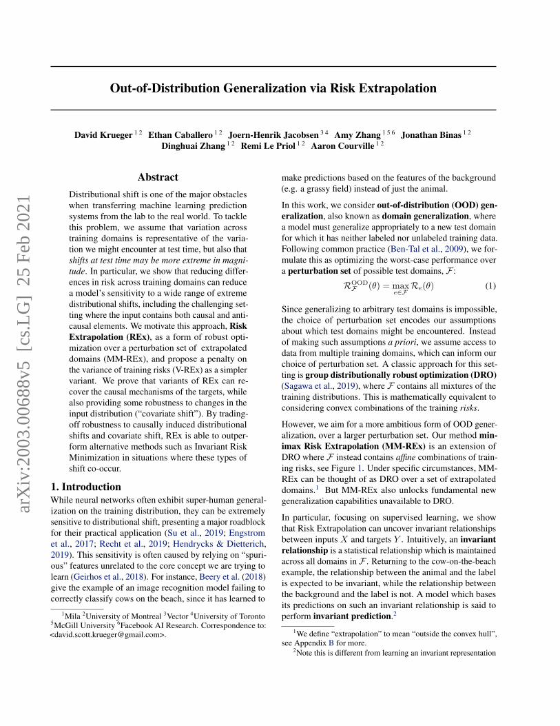
Figure 2. Training accuracies (left) and risks (right) on colored MNIST domains with varying P (Y = 0|color = red) after 500 epochs.Dots represent training risks, lines represent test risks on different domains. Increasing the V-REx penalty (β) leads to a flatter “risk plane”and more consistent performance across domains, as the model learns to ignore color in favor of shape-based invariant prediction. Notethat β = 100 gives the best worst-case risk across the 2 training domains, and so would be the solution preferred by DRO (Sagawa et al.,2019). This demonstrates that REx’s counter-intuitive propensity to increase training risks can be necessary for good OOD performance.

dom(Z) for each variable Z.4 Mechanisms are determinis-tic; noise in Z is represented explicitly via a special noisevariable NZ , and these noise variables are jointly indepen-dent. An intervention, ι is any modification to the mecha-nisms of one or more variables; an intervention can intro-duce new edges, so long as it does not introduce a cycle.do(Xi = x) denotes an intervention which sets Xi to theconstant value x (removing all incoming edges). Data canbe generated from an SCM, C, by sampling all of the noisevariables, and then using the mechanisms to compute thevalue of every node whose parents’ values are known. Thissampling process defines an entailed distribution, PC(Z)over the nodes Z of C. We overload fZ , letting fZ(Z) referto the conditional distribution PC(Z|Z \ {Z}).

2.3.1. CAUSAL APPROACHES TO DOMAINGENERALIZATION

Instead of assumingP (Y |X) is fixed (FRA), works that takea causal approach to domain generalization often assumethat the mechanism for Y is fixed; we call this the fixedmechanism assumption (FMA). Meanwhile, they assumeX may be subject to different (e.g. arbitrary) interventionsin different domains (Bühlmann, 2018). We call changes inP (X,Y ) resulting from interventions on X interventionalshift. Interventional shift can involve both covariate shiftand/or concept shift. In their seminal work on InvariantCausal Prediction (ICP), Peters et al. (2016) leverage thisinvariance to learn which elements of X cause Y . ICPand its nonlinear extension (Heinze-Deml et al., 2018) usestatistical tests to detect whether the residuals of a linearmodel are equal across domains. Our work differs from ICPin that:

1. Our method is model agnostic and scales to deep net-works.

4Our definitions follow Elements of Causal Inference (Peterset al., 2017); our notation mostly does as well.

2. Our goal is OOD generalization, not causal inference.These are not identical: invariant prediction can some-times make use of non-causal relationships, but whendeciding which interventions to perform, a truly causalmodel is called for.

3. Our learning principle only requires invariance of risks,not residuals. Nonetheless, we prove that this canensure invariant causal prediction.

A more similar method to REx is Invariant Risk Minimiza-tion (IRM) (Arjovsky et al., 2019), which shares properties(1) and (2) of the list above. Like REx, IRM also uses aweaker form of invariance than ICP; namely, they insist thatthe optimal linear classifier must match across domains.5

Still, REx differs significantly from IRM. While IRM specif-ically aims for invariant prediction, REx seeks robustnessto whichever forms of distributional shift are present. Thus,REx is more directly focused on the problem of OOD gen-eralization, and can provide robustness to a wider variety ofdistributional shifts, inluding covariate shift. Also, unlikeREx, IRM seeks to match E(Y |Φ(X)) across domains, notthe full P (Y |Φ(X)). This, combined with IRM’s indiffer-ence to covariate shift, make it more effective in cases wheredifferent domains or examples are inherently more noisy.

2.4. Fairness

Equalizing risk across different groups (e.g. male vs. fe-male) has been proposed as a definition of fairness (Doniniet al., 2018), generalizing the equal opportunity definition offairness (Hardt et al., 2016). Williamson & Menon (2019)propose using the absolute difference of risks to measure de-viation from this notion of fairness; this corresponds to ourMM-REx, in the case of only two domains, and is similar toV-REx, which uses the variance of risks. However, in thecontext of fairness, equalizing the risk of training groups is

5In practice, IRMv1 replaces this bilevel optimization problemwith a gradient penalty on classifier weights.


the goal. Our work goes beyond this by showing that it canserve as a method for OOD generalization.

3. Risk ExtrapolationBefore discussing algorithms for REx and theoretical results,we first expand on our high-level explanations of what RExdoes, what kind of OOD generalization it promotes, andhow. The principle of Risk Extrapolation (REx) has twoaims:

1. Reducing training risks

2. Increasing similarity of training risks

In general, these goals can be at odds with each other; de-creasing the risk in the domain with the lowest risk also de-creases the overall similarity of training risks. Thus methodsfor REx may seek to increase risk on the best performing do-mains. While this is counter-intuitive, it can be necessary toachieve good OOD generalization, as Figure 2 demonstrates.From a geometric point of view, encouraging equality ofrisks flattens the “risk plane” (the affine span of the trainingrisks, considered as a function of the data distribution, seeFigures 1 and 2). While this can result in higher trainingrisks, it also means that the risk changes less if the distribu-tional shifts between training domains are magnified at testtime.

Figure 2 illustrates how flattening the risk plane can promoteOOD generalization on real data, using the Colored MNIST(CMNIST) task as an example (Arjovsky et al., 2019). Inthe CMNIST training domains, the color of a digit is morepredictive of the label than the shape is. But because the cor-relation between color and label is not invariant, predictorsthat use the color feature achieve different risk on differentdomains. By enforcing equality of risks, REx prevents themodel from using the color feature enabling successful gen-eralization to the test domain where the correlation betweencolor and label is reversed.

Probabilities vs. Risks. Figure 3 depicts how the extrap-olated risks considered in MM-REx can be translated intoa corresponding change in P (X,Y ), using an example ofpure covariate shift. Training distributions can be thoughtof as points in an affine space with a dimension for everypossible value of (X,Y ); see Appendix C.1 for an example.Because the risk is linear w.r.t. P (x, y), a convex combi-nation of risks from different domains is equivalent to therisk on a domain given by the mixture of their distributions.The same holds for the affine combinations used in MM-REx, with the caveat that the negative coefficients may leadto negative probabilities, making the resulting P (X,Y ) aquasiprobability distribution, i.e. a signed measure withintegral 1. We explore the theoretical implications of this inAppendix E.

x

P(x)

Pe1(x)Pe2(x)

x

P(x)

interpolationextrapolation

Figure 3. Extrapolation can yield a distribution with negative P (x)for some x. Left: P (x) for domains e1 and e2. Right: Point-wiseinterpolation/extrapolation of P e1(x) and P e2(x). Since MM-REx target worst-case robustness across extrapolated domains, itcan provide robustness to such shifts in P(X) (covariate shift).

Covariate Shift. When only P (X) differs across do-mains (i.e. FRA holds), as in Figure 3, then Φ(x) = x is al-ready an equipredictive representation, and so any predictoris an invariant predictor. Thus methods which only promoteinvariant prediction – such as IRM – are not expected toimprove OOD generalization (compared with ERM). In-deed, Arjovsky et al. (2019) recognize this limitation ofIRM in what they call the “realizable” case. Instead, whatis needed is robustness to covariate shift, which REx, butnot IRM, can provide. Robustness to covariate shift canimprove OOD generalization by ensuring that low-capacitymodels spend sufficient capacity on low-density regions ofthe input space; we show how REx can provide such ben-efits in Appendix C.2. But even for high capacity models,P (X) can have a significant influence on what is learned;for instance Sagawa et al. (2019) show that DRO can sig-nificantly improves the performance on rare groups in theirwith a model that achieves 100% training accuracy in theirWaterbirds dataset. Pursuing robustness to covariate shiftalso comes with drawbacks for REx, however: REx does notdistinguish between underfitting and inherent noise in thedata, and so can force the model to make equally bad pre-dictions everywhere, even if some examples are less noisythan others.

3.1. Methods of Risk Extrapolation

We now formally describe the Minimax REx (MM-REx)and Variance-REx (V-REx) techniques for risk extrapola-tion. Minimax-REx performs robust learning over a per-turbation set of affine combinations of training risks withbounded coefficients:

RMM-REx(θ).= max

Σeλe=1λe≥λmin

m∑e=1

λeRe(θ) (6)

= (1−mλmin) maxeRe(θ) + λmin

m∑e=1

Re(θ) ,

(7)

where m is the number of domains, and the hyperparame-ter λmin controls how much we extrapolate. For negativevalues of λmin, MM-REx places negative weights on therisk of all but the worst-case domain, and as λmin → −∞,


this criterion enforces strict equality between training risks;λmin = 0 recovers risk interpolation (RI). Thus, like RI,MM-REx aims to be robust in the direction of variations inP (X,Y ) between test domains. However, negative coeffi-cients allow us to extrapolate to more extreme variations.Geometrically, larger values of λmin expand the perturba-tion set farther away from the convex hull of the trainingrisks, encouraging a flatter “risk-plane” (see Figure 2).

While MM-REx makes the relationship to RI/RO clear, wefound using the variance of risks as a regularizer (V-REx)simpler, stabler, and more effective:

RV-REx(θ).= β Var({R1(θ), ...,Rm(θ)}) +

m∑e=1

Re(θ)

(8)

Here β ∈ [0,∞) controls the balance between reducingaverage risk and enforcing equality of risks, with β = 0 re-covering ERM, and β →∞ leading V-REx to focus entirelyon making the risks equal. See Appendix for the relation-ship between V-REx and MM-REx and their gradient vectorfields.

3.2. Theoretical Conditions for REx to Perform CausalDiscovery

We now prove that exactly equalizing training risks (as in-centivized by REx) leads a model to learn the causal mecha-nism of Y under assumptions similar to those of Peters et al.(2016), namely:

1. The causes of Y are observed, i.e. Pa(Y ) ⊆ X .

2. Domains correspond to interventions on X .

3. Homoskedasticity (a slight generalization of the addi-tive noise setting assumed by Peters et al. (2016)). Wesay an SEM C is homoskedastic (with respect to a lossfunction `), if the Bayes error rate of `(fY (x), fY (x))is the same for all x ∈ X .6

The contribution of our theory (vs. ICP) is to prove thatequalizing risks is sufficient to learn the causes of Y . In con-trast, they insist that the entire distribution of error residuals(in predicting Y ) be the same across domains. We provideproof sketches here and complete proofs in the appendix.

Theorem 1 demonstrates a practical result: we can identifya linear SEM model using REx with a number of domainslinear in the dimensionality of X.

6 Note that our definitions of homoskedastic/heteroskedasticdo not correspond to the types of domains constructed in Arjovskyet al. (2019), Section 5.1, but rather are a generalization of thedefinitions of these terms as commonly used in statistics. Specif-ically, for us, heteroskedasticity means that the “predicatability”(e.g. variance) of Y differs across inputs x, whereas for Arjovskyet al. (2019), it means the predicatability of Y at a given inputvaries across domains; we refer to this second type as domain-homo/heteroskedasticity for clarity.

Theorem 1. Given a Linear SEM, Xi ←∑j 6=i β(i,j)Xj +

εi, with Y .= X0, and a predictor fβ(X)

.=∑j:j>0 βjXj+

εj that satisfies REx (with mean-squared error) over a per-turbation set of domains that contains 3 distinct do() inter-ventions for each Xi : i > 0. Then βj = β0,j ,∀j.Proof Sketch. We adapt the proof of Theorem 4i fromPeters et al. (2016). They show that matching the resid-ual errors across observational and interventional domainsforces the model to learn fY . We use the weaker conditionof matching risks to derive a quadratic equation that thedo() interventions must satisfy for any model other thanfY . Since there are at most 2 solutions to a quadratic equa-tion, insisting on equality of risks across 3 distinct do()interventions forces the model to learn fY .

Given the assumption that a predictor satisfies REx over allinterventions that do not change the mechanism of Y , wecan prove a much more general result. We now consider anarbitrary SCM, C, generating Y and X , and let EI be theset of domains corresponding to arbitrary interventions onX , similarly to Peters et al. (2016).

Theorem 2. Suppose ` is a (strictly) proper scoring rule.Then a predictor that satisfies REx for a over EI uses fY (x)as its predictive distribution on input x for all x ∈ X .

Proof Sketch. Since the distribution of Y given its par-ents doesn’t depend on the domain, fY can make reliablepoint-wise predictions across domains. This translates intoequality of risk across domains when the overall difficultyof the examples is held constant across domains, e.g. byassuming homoskedasticity.7 While a different predictormight do a better job on some domains, we can always findan domain where it does worse than fY , and so fY is bothunique and optimal.

Remark. Theorem 2 is only meant to provide insight intohow the REx principle relates to causal invariance; the per-turbation set in this theorem is uncountably infinite. Note,however, that even in this setting, the ERM principle doesnot, in general, recover the causal mechanism for Y . Rather,the ERM solution depends on the distribution over domains.For instance, if all but an ε→ 0 fraction of the data comesfrom the CMNIST training domains, then ERM will learnto use the color feature, just as in original the CMNIST task.

4. ExperimentsWe evaluate REx and compare with IRM on a range oftasks requiring OOD generalization. REx provides gener-alization benefits and outperforms IRM on a wide range oftasks, including: i) variants of the Colored MNIST (CM-NIST) dataset (Arjovsky et al., 2019) with covariate shift,ii) continuous control tasks with partial observability and

7Note we could also assume no covariate shift in order to fixthe difficulty, but this seems hard to motivate in the context ofinterventions on X , which can change P (X).


0.00.10.20.30.40.5p = P(shape(x) {0,1,2,3,4})

0.2

0.3

0.4

0.5

0.6

Test

Acc

urac

y

Random GuessingV-RExIRMv1

0.00.10.20.30.40.5p = P(shape(x) {1,2} {6,7})

0.2

0.3

0.4

0.5

0.6

Test

Acc

urac

y


0.00.10.20.30.40.5p = P(R1|Red) = P(G1|Green)

0.1

0.2

0.3

0.4

0.5

0.6

Test

Acc

urac

y


Figure 4. REx outperforms IRM on Colored MNIST variants that include covariate shift. The x-axis indexes increasing amount of shiftbetween training distributions, with p = 0 corresponding to disjoint supports. Left: class imbalance, Center: shape imbalance, Right:color imbalance.

Method train acc test acc

V-REx (ours) 71.5± 1.0 68.7± 0.9IRM 70.8± 0.9 66.9± 2.5MM-REx (ours) 72.4± 1.8 66.1± 1.5RI 88.9± 0.3 22.3± 4.6ERM 87.4± 0.2 17.1± 0.6

Grayscale oracle 73.5± 0.2 73.0± 0.4Optimum 75 75Chance 50 50

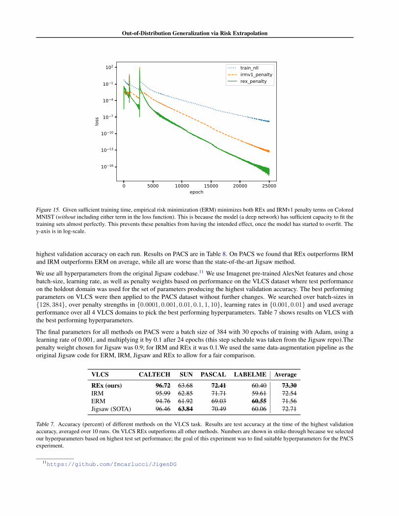
Table 2. Accuracy (percent) on ColoredMNIST. REx and IRM learn to ignore the spurious colorfeature. Strikethrough results achieved via tuning on the test set.

spurious features, iii) domain generalization tasks from theDomainBed suite (Gulrajani & Lopez-Paz, 2020). On theother hand, when the inherent noise in Y varies across envi-ronments, IRM succeeds and REx performs poorly.

4.1. Colored MNISTArjovsky et al. (2019) construct a binary classification prob-lem (with 0-4 and 5-9 each collapsed into a single class)based on the MNIST dataset, using color as a spurious fea-ture. Specifically, digits are either colored red or green,and there is a strong correlation between color and label,which is reversed at test time. The goal is to learn the causal“digit shape” feature and ignore the anti-causal “digit color”feature. The learner has access to three domains:

1. A training domain where green digits have a 80%chance of belonging to class 1 (digits 5-9).

2. A training domain where green digits have a 90%chance of belonging to class 1.

3. A test domain where green digits have a 10% chanceof belonging to class 1.

We use the exact same hyperparameters as Arjovsky et al.(2019), only replacing the IRMv1 penalty with MM-REx orV-REx penalty.8 These methods all achieve similar perfor-

8When there are only 2 domains, MM-REx is equivalent to a

mance, see Table 2.

CMNIST with covariate shift. To test our hypothesis thatREx should outperform IRM under covariate shift, we con-struct 3 variants of the CMNIST dataset. Each variant repre-sents a different way of inducing covariate shift to ensuredifferences across methods are consistent. These exper-iments combine covariate shift with interventional shift,since P (Green|Y = 1) still differs across training domainsas in the original CMNIST.

1. Class imbalance: varying p = P (shape(x) ∈{0, 1, 2, 3, 4}); as in Wu et al. (2020).

2. Digit imbalance: varying p = P (shape(x) ∈{1, 2} ∪ {6, 7}); digits 0 and 5 are removed.

3. Color imbalance: We use 2 versions of each color,for 4 total channels: R1, R2, G1, G2. We vary p =P (R1|Red) = P (G1|Green).

While (1) also induces change in P (Y ), (2) and (3) induceonly covariate shift in the causal shape and anti-causal colorfeatures (respectively). We compare across several levelsof imbalance, p ∈ [0, 0.5], using the same hyperparametersfrom Arjovsky et al. (2019), and plot the mean and standarderror over 3 trials.

V-REx significantly outperforms IRM in every case, seeFigure 3.2. In order to verify that these results are not dueto bad hyperparameters for IRM, we perform a randomsearch that samples 340 unique hyperparameter combina-tions for each value of p, and compare the the number oftimes each method achieves better than chance-level (50%accuracy). Again, V-REx outperforms IRM; in particu-lar, for small values of p, IRM never achieves better thanrandom chance performance, while REx does better thanrandom in 4.4%/23.7%/2.0% of trials, respectively, in theclass/digit/color imbalance scenarios for p = 0.1/0.1/0.2.This indicates that REx can achieve good OOD generaliza-tion in settings involving both covariate and interventionalshift, whereas IRM struggles to do so.

penalty on the Mean Absolute Error (MAE), see Appendix F.2.2.


0.0 0.1 0.2 0.3 0.4 0.5 0.6 0.7 0.8 0.9 1.0step 1e5

50

100

150

200

250

300

Episo

de R

ewar

d

ERMIRMREx

0.0 0.1 0.2 0.3 0.4 0.5 0.6 0.7 0.8 0.9 1.0step 1e5

0

100

200

300

400

500

600

700

800

Episo

de R

ewar

d

ERMIRMREx

Figure 5. Performance and standard error on walker_walk (top), finger_spin (bottom).

Algorithm ColoredMNIST VLCS PACS OfficeHome

ERM 52.0 ± 0.1 77.4 ± 0.3 85.7 ± 0.5 67.5 ± 0.5IRM 51.8 ± 0.1 78.1 ± 0.0 84.4 ± 1.1 66.6 ± 1.0

V-REx 52.1 ± 0.1 77.9 ± 0.5 85.8 ± 0.6 66.7 ± 0.5

Table 3. REx, IRM, and ERM all perform comparably on a set of domain generalization benchmarks.

4.2. Toy Structural Equation Models (SEMs)

REx’s sensitivity to covariate shift can also be a weaknesswhen reallocating capacity towards domains with higherrisk does not help the model reduce their risk, e.g. due to ir-reducible noise. We illustrate this using the linear-Gaussianstructural equation model (SEM) tasks introduced by Ar-jovsky et al. (2019). Like CMNIST, these SEMs includespurious features by construction. They also introduce 1)heteroskedasticity, 2) hidden confounders, and/or 3) ele-ments of X that contain a mixture of causes and effects ofY . These three properties highlight advantages of IRM overICP (Peters et al., 2016), as demonstrated empirically byArjovsky et al. (2019). REx is also able to handle (2) and(3), but it performs poorly in the heteroskedastic tasks. SeeAppendix G.2 for details and Table 5 for results.

4.3. Domain Generalization in the DomainBed Suite

Methodologically, it is inappropriate to assume access to thetest environment in domain generalization settings, as thegoal is to find methods which generalize to unknown testdistributions. Gulrajani & Lopez-Paz (2020) introduced theDomainBed evaluation suite to rigorously compare existingapproaches to domain generalization, and found that nomethod reliably outperformed ERM. We evaluate V-RExon DomainBed using the most commonly used training-domain validation set method for model selection. Dueto limited computational resources, we limited ourselvesto the 4 cheapest datasets. Results of baseline are takenfrom Gulrajani & Lopez-Paz (2020), who compare withmore methods. Results in Table 3 give the average over 3different train/valid splits.

4.4. Reinforcement Learning with partial observabilityand spurious features

Finally, we turn to reinforcement learning, where covariateshift (potentially favoring REx) and heteroskedasticity(favoring IRM) both occur naturally as a result of ran-domness in the environment and policy. In order to showthe benefits of invariant prediction, we modify tasksfrom the Deepmind Control Suite (Tassa et al., 2018) toinclude spurious features in the observation, and traina Soft Actor-Critic (Haarnoja et al., 2018) agent. RExoutperforms both IRM and ERM, suggesting that REx’srobustness to covariate shift outweighs the challenges itfaces with heteroskedasticity in this setting, see Figure 5.We average over 10 runs on finger_spin andwalker_walk, using hyperparameters tuned oncartpole_swingup (to avoid overfitting). SeeAppendix for details and further results.

5. ConclusionWe have demonstrated that REx, a method for robustoptimization, can provide robustness and hence out-of-distribution generalization in the challenging case whereX contains both causes and effects of Y . In particular, likeIRM, REx can perform causal identification, but REx canalso perform more robustly in the presence of covariate shift.Covariate shift is known to be problematic when modelsare misspecified, when training data is limited, or does notcover areas of the test distribution. As such situations areinevitable in practice, REx’s ability to outperform IRM inscenarios involving a combination of covariate shift andinterventional shift makes it a powerful approach.


ReferencesAlbuquerque, I., Naik, N., Li, J., Keskar, N., and Socher,

R. Improving out-of-distribution generalization via multi-task self-supervised pretraining, 2020.

Arjovsky, M., Bottou, L., Gulrajani, I., and Lopez-Paz, D. Invariant risk minimization. arXiv preprintarXiv:1907.02893, 2019.

Bachman, P., Hjelm, R. D., and Buchwalter, W. Learningrepresentations by maximizing mutual information acrossviews, 2019.

Bagnell, J. A. Robust supervised learning. In Proceedingsof the 20th National Conference on Artificial Intelligence- Volume 2, AAAI’05, pp. 714–719. AAAI Press, 2005.ISBN 157735236x.

Beery, S., Van Horn, G., and Perona, P. Recognition interra incognita. Lecture Notes in Computer Science, pp.472–489, 2018. ISSN 1611-3349.

Ben-David, S., Blitzer, J., Crammer, K., Kulesza, A.,Pereira, F., and Vaughan, J. W. A theory of learning fromdifferent domains. Machine learning, 79(1-2):151–175,2010a.

Ben-David, S., Lu, T., Luu, T., and Pál, D. Impossibilitytheorems for domain adaptation. In Proceedings of theThirteenth International Conference on Artificial Intelli-gence and Statistics, pp. 129–136, 2010b.

Ben-Tal, A., El Ghaoui, L., and Nemirovski, A. Robustoptimization, volume 28. Princeton University Press,2009.

Bühlmann, P. Invariance, causality and robustness, 2018.

Carlucci, F. M., D’Innocente, A., Bucci, S., Caputo, B., andTommasi, T. Domain generalization by solving jigsawpuzzles. In Proceedings of the IEEE Conference on Com-puter Vision and Pattern Recognition, pp. 2229–2238,2019.

Cubuk, E. D., Zoph, B., Mane, D., Vasudevan, V., and Le,Q. V. Autoaugment: Learning augmentation policiesfrom data, 2018.

Desjardins, G., Simonyan, K., Pascanu, R., et al. Naturalneural networks. In Advances in Neural InformationProcessing Systems, pp. 2071–2079, 2015.

Donini, M., Oneto, L., Ben-David, S., Shawe-Taylor, J., andPontil, M. Empirical risk minimization under fairnessconstraints, 2018.

Engstrom, L., Tran, B., Tsipras, D., Schmidt, L., and Madry,A. Exploring the landscape of spatial robustness. arXivpreprint arXiv:1712.02779, 2017.

Ganin, Y., Ustinova, E., Ajakan, H., Germain, P., Larochelle,H., Laviolette, F., Marchand, M., and Lempitsky, V.Domain-adversarial training of neural networks. TheJournal of Machine Learning Research, 17(1):2096–2030,2016.

Geirhos, R., Rubisch, P., Michaelis, C., Bethge, M., Wich-mann, F. A., and Brendel, W. Imagenet-trained cnns arebiased towards texture; increasing shape bias improves ac-curacy and robustness. arXiv preprint arXiv:1811.12231,2018.

Goodfellow, I. J., Shlens, J., and Szegedy, C. Explain-ing and harnessing adversarial examples. arXiv preprintarXiv:1412.6572, 2014.

Gowal, S., Qin, C., Huang, P.-S., Cemgil, T., Dvijotham, K.,Mann, T., and Kohli, P. Achieving robustness in the wildvia adversarial mixing with disentangled representations.arXiv preprint arXiv:1912.03192, 2019.

Gulrajani, I. and Lopez-Paz, D. In search of lost domaingeneralization, 2020.

Haarnoja, T., Zhou, A., Abbeel, P., and Levine, S. Softactor-critic: Off-policy maximum entropy deep reinforce-ment learning with a stochastic actor. In Dy, J. andKrause, A. (eds.), Proceedings of the 35th InternationalConference on Machine Learning, volume 80 of Pro-ceedings of Machine Learning Research, pp. 1861–1870,Stockholmsmässan, Stockholm Sweden, 10–15 Jul 2018.PMLR.

Haffner, P. Escaping the convex hull with extrapolatedvector machines. In Dietterich, T. G., Becker, S., andGhahramani, Z. (eds.), Advances in Neural InformationProcessing Systems 14, pp. 753–760. MIT Press, 2002.

Hardt, M., Price, E., and Srebro, N. Equality of opportunityin supervised learning, 2016.

Hastie, T., Tibshirani, R., and Friedman, J. The elements ofstatistical learning: data mining, inference, and predic-tion. Springer Science & Business Media, 2009.

He, Y., Shen, Z., and Cui, P. Towards non-i.i.d. imageclassification: A dataset and baselines, 2019.

Heinze-Deml, C., Peters, J., and Meinshausen, N. Invari-ant causal prediction for nonlinear models. Journal ofCausal Inference, 6(2), Sep 2018. ISSN 2193-3685. doi:10.1515/jci-2017-0016. URL http://dx.doi.org/10.1515/jci-2017-0016.

Hendrycks, D. and Dietterich, T. Benchmarking neuralnetwork robustness to common corruptions and perturba-tions. arXiv preprint arXiv:1903.12261, 2019.

http://dx.doi.org/10.1515/jci-2017-0016

http://dx.doi.org/10.1515/jci-2017-0016


Hendrycks, D. and Gimpel, K. A baseline for detectingmisclassified and out-of-distribution examples in neuralnetworks. arXiv preprint arXiv:1610.02136, 2016.

Hendrycks, D., Mazeika, M., and Dietterich, T. Deepanomaly detection with outlier exposure. arXiv preprintarXiv:1812.04606, 2018.

Hendrycks, D., Mazeika, M., Kadavath, S., and Song, D.Using self-supervised learning can improve model robust-ness and uncertainty, 2019a.

Hendrycks, D., Mu, N., Cubuk, E. D., Zoph, B., Gilmer,J., and Lakshminarayanan, B. Augmix: A simple dataprocessing method to improve robustness and uncertainty,2019b.

Hjelm, R. D., Fedorov, A., Lavoie-Marchildon, S., Grewal,K., Bachman, P., Trischler, A., and Bengio, Y. Learningdeep representations by mutual information estimationand maximization, 2018.

Hu, W., Niu, G., Sato, I., and Sugiyama, M. Does distribu-tionally robust supervised learning give robust classifiers?,2016.

Ilse, M., Tomczak, J. M., and Forré, P. Designing dataaugmentation for simulating interventions. arXiv preprintarXiv:2005.01856, 2020.

Johansson, F. D., Sontag, D., and Ranganath, R. Support andinvertibility in domain-invariant representations, 2019.

Koyama, M. and Yamaguchi, S. Out-of-distribution gener-alization with maximal invariant predictor, 2020.

Krizhevsky, A., Sutskever, I., and Hinton, G. E. Imagenetclassification with deep convolutional neural networks.In Advances in neural information processing systems,pp. 1097–1105, 2012.

Li, D., Yang, Y., Song, Y.-Z., and Hospedales, T. M. Deeper,broader and artier domain generalization. In Proceedingsof the IEEE international conference on computer vision,pp. 5542–5550, 2017.

Li, Y., Tian, X., Gong, M., Liu, Y., Liu, T., Zhang, K.,and Tao, D. Deep domain generalization via conditionalinvariant adversarial networks. In Proceedings of theEuropean Conference on Computer Vision (ECCV), pp.624–639, 2018.

Lipton, Z. C., Wang, Y.-X., and Smola, A. Detecting andcorrecting for label shift with black box predictors. arXivpreprint arXiv:1802.03916, 2018.

Long, M., Cao, Z., Wang, J., and Jordan, M. I. Conditionaladversarial domain adaptation. In Advances in NeuralInformation Processing Systems, pp. 1640–1650, 2018.

Meinshausen, N., Bühlmann, P., et al. Maximin effects ininhomogeneous large-scale data. The Annals of Statistics,43(4):1801–1830, 2015.

Pan, S. J., Tsang, I. W., Kwok, J. T., and Yang, Q. Do-main adaptation via transfer component analysis. IEEETransactions on Neural Networks, 22(2):199–210, 2010.

Peters, J., Bühlmann, P., and Meinshausen, N. Causal in-ference by using invariant prediction: identification andconfidence intervals. Journal of the Royal Statistical Soci-ety: Series B (Statistical Methodology), 78(5):947–1012,2016.

Peters, J., Janzing, D., and Schölkopf, B. Elements of causalinference: foundations and learning algorithms. 2017.

Recht, B., Roelofs, R., Schmidt, L., and Shankar, V. Do im-agenet classifiers generalize to imagenet? arXiv preprintarXiv:1902.10811, 2019.

Sagawa, S., Koh, P. W., Hashimoto, T. B., and Liang, P.Distributionally robust neural networks for group shifts:On the importance of regularization for worst-case gener-alization, 2019.

Sahoo, S. S., Lampert, C. H., and Martius, G. Learningequations for extrapolation and control, 2018.

Schölkopf, B., Janzing, D., Peters, J., Sgouritsa, E., Zhang,K., and Mooij, J. On causal and anticausal learning. InProceedings of the 29th International Coference on Inter-national Conference on Machine Learning, ICML’12, pp.459–466, Madison, WI, USA, 2012. Omnipress. ISBN9781450312851.

Shorten, C. and Khoshgoftaar, T. M. A survey on imagedata augmentation for deep learning. Journal of Big Data,6(1):60, 2019.

Sinha, A., Namkoong, H., Volpi, R., and Duchi, J. Cer-tifying some distributional robustness with principledadversarial training, 2017.

Su, J., Vargas, D. V., and Sakurai, K. One pixel attackfor fooling deep neural networks. IEEE Transactions onEvolutionary Computation, 23(5):828–841, 2019.

Tassa, Y., Doron, Y., Muldal, A., Erez, T., Li, Y.,de Las Casas, D., Budden, D., Abdolmaleki, A., Merel, J.,Lefrancq, A., Lillicrap, T., and Riedmiller, M. DeepMindcontrol suite. Technical report, DeepMind, January 2018.

Tian, Y., Krishnan, D., and Isola, P. Contrastive multiviewcoding, 2019.

Torralba, A. and Efros, A. A. Unbiased look at dataset bias.In CVPR 2011, pp. 1521–1528. IEEE, 2011.


Tzeng, E., Hoffman, J., Saenko, K., and Darrell, T. Adver-sarial discriminative domain adaptation. In Proceedingsof the IEEE Conference on Computer Vision and PatternRecognition, pp. 7167–7176, 2017.

van den Oord, A., Li, Y., and Vinyals, O. Representationlearning with contrastive predictive coding, 2018.

Wang, H., He, Z., Lipton, Z. C., and Xing, E. P. Learningrobust representations by projecting superficial statisticsout. arXiv preprint arXiv:1903.06256, 2019.

Williamson, R. C. and Menon, A. K. Fairness risk measures,2019.

Wu, X., Guo, Y., Chen, J., Liang, Y., Jha, S., and Chalasani,P. Representation bayesian risk decompositions and multi-source domain adaptation, 2020.

Zhang, C., Bengio, S., Hardt, M., Recht, B., and Vinyals, O.Understanding deep learning requires rethinking general-ization. arXiv preprint arXiv:1611.03530, 2016.

Zhang, H., Cisse, M., Dauphin, Y. N., and Lopez-Paz, D.mixup: Beyond empirical risk minimization, 2017.

Zhao, H., des Combes, R. T., Zhang, K., and Gordon, G. J.On learning invariant representation for domain adapta-tion, 2019.


Appendices


A. Appendix OverviewOur code is available online at: https://anonymous.4open.science/r/12747e81-8505-43cb-b54e-e75e2344a397/. The sectionsof our appendix are as follows:

A) Appendix Overview

B) Definition and discussion of extrapolation in machine learning

C) Illustrative examples of how REx works in toy settings

D) A summary of different types of causal model

E) Theory

F) The relationship between MM-REx vs. V-REx, and the role each plays in our work

G) Further results and details for experiments mentioned in main text

H) Experiments not mentioned in main text

I) Overview of other topics related to OOD generalization

B. Definition and discussion of extrapolation in machine learningWe define interpolation and extrapolation as follows: interpolation refers to making decisions or predictions about pointswithin the convex hull of the training examples and extrapolation refers to making decisions or predictions about pointsoutside their convex hull.9 This generalizes the familiar sense of these terms for one-dimensional functions. An interestingconsequence of this definition is: for data of high intrinsic dimension, generalization requires extrapolation (Hastie et al.,2009), even in the i.i.d. setting. This is because the volume of high-dimensional manifolds concentrates near their boundary;see Figure 6.

Extrapolation in the space of risk functions. The same geometric considerations apply to extrapolating to new domains.Domains can be highly diverse, varying according to high dimensional attributes, and thus requiring extrapolation togeneralize across. Thus Risk Extrapolation might often do a better job of including possible test domains in its perturbationset than Risk Interpolation does.

Training points

Test point

Figure 6. Illustration of the importance of extrapolation for generalizing in high dimensional space. In high dimensional spaces, massconcentrates near the boundary of objects. For instance, the uniform distribution over a ball in N + 1-dimensional space can beapproximated by the uniform distribution over the N -dimensional hypersphere. We illustrate this in 2 dimensions, using the 1-sphere (i.e.the unit circle). Dots represent a finite training sample, and the shaded region represents the convex hull of all but one member of thesample. Even in 2 dimensions, we can see why any point from a finite sample from such a distribution remains outside the convex hull ofthe other samples, with probability 1. The only exception would be if two points in the sample coincide exactly.

9Surprisingly, we were not able to find any existing definition of these terms in the machine learning literature. They have been used inthis sense (Hastie et al., 2009; Haffner, 2002), but also to refer to strong generalization capabilities more generally (Sahoo et al., 2018).

https://anonymous.4open.science/r/12747e81-8505-43cb-b54e-e75e2344a397/


C. Illustrative examples of how REx works in toy settingsHere, we work through two examples to illustrate:

1. How to understand extrapolation in the space of probability density/mass functions (PDF/PMFs)

2. How REx encourages robustness to covariate shift via distributing capacity more evenly across possible input distribu-tions.

C.1. 6D example of REx

Here we provide a simple example illustrating how to understand extrapolations of probability distributions. SupposeX ∈ {0, 1, 2} and Y ∈ {0, 1}, so there are a total of 6 possible types of examples, and we can represent their distributionsin a particular domain as a point in 6D space: (P (0, 0), P (0, 1), P (1, 0), P (1, 1), P (2, 0), P (2, 1)). Now, consider threedomains e1, e2, e3 given by

1. (a, b, c, d, e, f)

2. (a, b, c, d, e− k, f + k)

3. (2a, 2b, c(1− a+bc+d ), d(1− a+b

c+d ), e, f)

The difference between e1 and e2 corresponds to a shift in P (Y |X = 2), and suggests that Y cannot be reliably predictedacross different domains when X = 2. Meanwhile, the difference between e1 and e3 tells us that the relative probability ofX = 0 vs. X = 1 can change, and so we might want our model to be robust to these sorts of covariate shifts. Extrapolatingrisks across these 3 domains effectively tells the model: “don’t bother trying to predict Y when X = 2 (i.e. aim forP (Y = 1|X = 2) = .5), and split your capacity equally across the X = 0 and X = 1 cases”. By way of comparison,IRM would also aim for P (Y = 1|X = 2) = .5, whereas ERM would aim for P (Y = 1|X = 2) = 3f+k

3e+3f (assuming|D1| = |D2| = |D3|). And unlike REx, both ERM and IRM would split capacity between X = 0/1/2 cases according totheir empirical frequencies.

C.2. Covariate shift example

We now give an example to show how REx provides robustness to covariate shift. Covariate shift is an issue when a modelhas limited capacity or limited data.

Viewing REx as robust learning over the affine span of the training distributions reveals its potential to improve robustness todistribution shifts. Consider a situation in which a model encounters two types of inputs: COSTLY inputs with probabilityq and CHEAP inputs with probability 1− q. The model tries to predicts the input – it outputs COSTLY with probabilityp and CHEAP with probability 1 − p. If the model predicts right its risk is 0, but if it predicts COSTLY instead ofCHEAP it gets a risk u = 2, and if it predicts CHEAP instead of COSTLY it gets a risk v = 4. The risk has expectationRq(p) = (1 − p)(1 − q)u + pqv. We have access to two domains with different input probabilities q1 < q2. This is anexample of pure covariate shift.

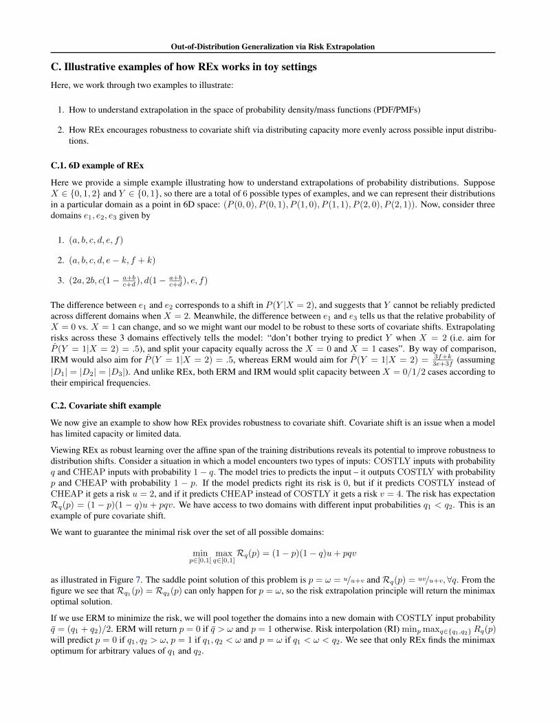
We want to guarantee the minimal risk over the set of all possible domains:

minp∈[0,1]

maxq∈[0,1]

Rq(p) = (1− p)(1− q)u+ pqv

as illustrated in Figure 7. The saddle point solution of this problem is p = ω = u/u+v andRq(p) = uv/u+v,∀q. From thefigure we see thatRq1(p) = Rq2(p) can only happen for p = ω, so the risk extrapolation principle will return the minimaxoptimal solution.

If we use ERM to minimize the risk, we will pool together the domains into a new domain with COSTLY input probabilityq = (q1 + q2)/2. ERM will return p = 0 if q > ω and p = 1 otherwise. Risk interpolation (RI) minp maxq∈{q1,q2}Rq(p)will predict p = 0 if q1, q2 > ω, p = 1 if q1, q2 < ω and p = ω if q1 < ω < q2. We see that only REx finds the minimaxoptimum for arbitrary values of q1 and q2.


0.0 0.2 0.4 0.6 0.8 1.0p

0.0

0.5

1.0

1.5

2.0

2.5

3.0

3.5

4.0 Rq(p)R (p)max

q Rq(p)( , R( ))

Figure 7. Each grey line is a riskRq(p) as functions of p for a specific value of q. The blue line is when q = ω. We highlight in red thecurve maxqRq(p) whose minimum is the saddle point marked by a purple star in p = ω.

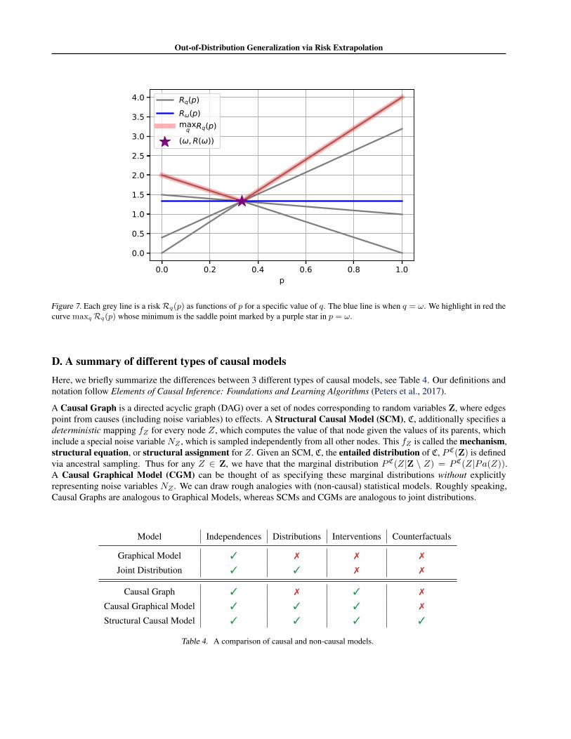
D. A summary of different types of causal modelsHere, we briefly summarize the differences between 3 different types of causal models, see Table 4. Our definitions andnotation follow Elements of Causal Inference: Foundations and Learning Algorithms (Peters et al., 2017).

A Causal Graph is a directed acyclic graph (DAG) over a set of nodes corresponding to random variables Z, where edgespoint from causes (including noise variables) to effects. A Structural Causal Model (SCM), C, additionally specifies adeterministic mapping fZ for every node Z, which computes the value of that node given the values of its parents, whichinclude a special noise variable NZ , which is sampled independently from all other nodes. This fZ is called the mechanism,structural equation, or structural assignment for Z. Given an SCM, C, the entailed distribution of C, PC(Z) is definedvia ancestral sampling. Thus for any Z ∈ Z, we have that the marginal distribution PC(Z|Z \ Z) = PC(Z|Pa(Z)).A Causal Graphical Model (CGM) can be thought of as specifying these marginal distributions without explicitlyrepresenting noise variables NZ . We can draw rough analogies with (non-causal) statistical models. Roughly speaking,Causal Graphs are analogous to Graphical Models, whereas SCMs and CGMs are analogous to joint distributions.

Model Independences Distributions Interventions Counterfactuals

Graphical Model 3 7 7 7

Joint Distribution 3 3 7 7

Causal Graph 3 7 3 7

Causal Graphical Model 3 3 3 7

Structural Causal Model 3 3 3 3

Table 4. A comparison of causal and non-causal models.


E. TheoryE.1. Proofs of theorems 1 and 2

The REx principle (Section 3) has two goals:

1. Reducing training risks

2. Increasing similarity of training risks.

In practice, it may be advantageous to trade-off these two objectives, using a hyperparameter (e.g. β for V-REx or λmin forMM-REx). However, in this section, we assume the 2nd criteria takes priority; i.e. we define “satisfying” the REx principleas selecting a minimal risk predictor among those that achieve exact equality of risks across all the domains in a set E .

Recall our assumptions from Section 3.2 of the main text:

1. The causes of Y are observed, i.e. Pa(Y ) ⊆ X .

2. Domains correspond to interventions on X .

3. Homoskedasticity (a slight generalization of the additive noise setting assumed by Peters et al. (2016)). We say anSEM C is homoskedastic (with respect to a loss function `), if the Bayes error rate of `(fY (x), fY (x)) is the same forall x ∈ X .

And see Section 2.3 for relevant definitions and notation.

We begin with a theorem based on the setting explored by Peters et al. (2016). Here, εi.= Ni are assumed to be normally

distributed.

Theorem 1. Given a Linear SEM, Xi ←∑j 6=i β(i,j)Xj + εi, with Y .

= X0, and a predictor fβ(X).=∑j:j>0 βjXj + εj

that satisfies REx (with mean-squared error) over a perturbation set of domains that contains 3 distinct do() interventionsfor each Xi : i > 0. Then βj = β0,j ,∀j.

Proof. We adapt the proof of Theorem 4i from Peters et al. (2016) to show that REx will learn the correct model undersimilar assumptions. Let Y ← γX + ε be the mechanism for Y , assumed to be fixed across all domains, and let Y = βX beour predictor. Then the residual is R(β) = (γ − β)X + ε. Define αi

.= γi − βi, and consider an intervention do(Xj = x)

on the youngest node Xj with αj 6= 0. Then as in eqn 36/37 of Peters et al. (2016), we compare the residuals R of thisintervention and of the observational distribution:

Robs(β) = αjXj +∑i 6=j

αiXi + ε Rdo(Xj=x)(β) = αjx+∑i 6=j

αiXi + ε (9)

We now compute the MSE risk for both domains, set them equal, and simplify to find a quadratic formula for x:

E

(αjXj +∑i 6=j

αiXi + ε)2

= E

(αjx+∑i 6=j

αiXi + ε)2

(10)

0 = α2jx

2 + 2αjE[∑i6=j

αiXi + ε]x− E

(αjXj)2 − 2αjXj(

∑i 6=j

αiXi + ε)

(11)

Since there are at most two values of x that satisfy this equation, any other value leads to a violation of REx, so that αjneeds to be zero – contradiction. In particular having domains with 3 different do-interventions on every Xi guarantees thatthe risks are not equal across all domains.


Given the assumption that a predictor satisfies REx over all interventions that do not change the mechanism of Y , we canprove a much more general result. We now consider an arbitrary SCM, C, generating Y and X , and let EI be the set ofdomains corresponding to arbitrary interventions on X , similarly to Peters et al. (2016).

We emphasize that the predictor is not restricted to any particular class of models, and is a generic function f : X → P(Y ),where P(Y ) is the set of distributions over Y . Hence, we drop θ from the below discussion and simply use f to representthe predictor, andR(f) its risk.Theorem 2. Suppose ` is a (strictly) proper scoring rule. Then a predictor that satisfies REx for a over EI uses fY (x) as itspredictive distribution on input x for all x ∈ X .

Proof. LetRe(f, x) be the loss of predictor f on point x in domain e, andRe(f) =∫P e(x)

Re(f, x) be the risk of f in e.

Define ι(x) as the domain given by the intervention do(X = x), and note that Rι(x)(f) = Rι(x)(f, x). We additionallydefine X1

.= Par(Y ).

The causal mechanism, fY , satisfies the REx principle over EI . For every x ∈ X , fY (x) = P (Y |do(X = x)) =P (Y |do(X1 = x1)) = P (Y |X1 = x1) is invariant (meaning ‘independent of domain’) by definition; P (Y |do(X = x)) =P (Y |do(X1 = x1)) = P (Y |X1 = x1) follows from the semantics of SEM/SCMs, and the fact that we don’t allow fYto change across domains. Specifically Y is always generated by the same ancestral sampling process that only dependson X1 and NY . Thus the risk of the predictor fY (x) at point x, Re(fY , x) = `(fY (x), fY (x)) is also invariant, soitR(fY , x). Thus Re(fY ) =

∫P e(x)

Re(fY , x) =∫P e(x)

R(fY , x) is invariant whenever R(fY , x) does not depend on x,and the homoskedasticity assumption ensures that this is the case. This establishes that setting f = fY will produce equalrisk across domains.

No other predictor satisfies the REx principle over EI . We show that any other g achieves higher risk than fY for at leastone domain. This demonstrates both that fY achieves minimal risk (thus satisfying REx), and that it is the unique predictorwhich does so (and thus no other predictors satisfy REx). We suppose such a g exists and construct an domain where itachieves higher risk than fY . Specifically, if g 6= fY then let x ∈ X be a point such that g(x) 6= fY (x). And since ` is astrictly proper scoring rule, this implies that `(g(x), fY (x)) > `(fY (x), fY (x)). But `(g(x), fY (x)) is exactly the risk of gon the domain ι(do(X = x)), and thus g achieves higher risk than fY in ι(do(X = x)), a contradiction.

E.2. REx as DRO

We note that MM-REx is also performing robust optimization over a convex hull, see Figure 1. The corners of thisconvex hull correspond to “extrapolated domains” with coefficients (λmin, λmin, ..., (1 − (m − 1)λmin)) (up to somepermutation). However, these domains do not necessarily correspond to valid probability distributions; in general, theyare quasidistributions, which can assign negative probabilities to some examples. This means that, even if the originalrisk functions were convex, the extrapolated risks need not be. However, in the case where they are convex, then existingtheorems, such as the convergence rate result of (Sagawa et al., 2019). This raises several important questions:

1. When is the affine combination of risks convex?

2. What are the effects of negative probabilities on the optimization problem REx faces, and the solutions ultimatelyfound?

Negative probabilities: Figure 8 illustrates this for a case where X = Z22, i.e. x is a binary vector of length 2.

Suppose x1, x2 are independent in our training domains, and represent the distribution for a particular domain by thepoint (P (X1 = 1), P (X2 = 1)). And suppose our 4 training distributions have (P (X1 = 1), P (X2 = 1)) equal to{(.4, .1), (.4, .9), (.6, .1), (.6, .9)}, with P (Y |X) fixed.

F. The relationship between MM-REx vs. V-REx, and the role each plays in our workThe MM-REx and V-REx methods play different roles in our work:

• We use MM-REx to illustrate that REx can be instantiated as a variant of robust optimization, specifically a generaliza-tion of the common Risk Interpolation approach. We also find MM-REx provides a useful geometric intuition, sincewe can visualize its perturbation set as an expansion of the convex hull of the training risks or distributions.


0.00.0

0.5

0.5

1.0

1.0

P (X1 = 1)P(X

2=

1) Training environments

Valid distributions

Perturbation set

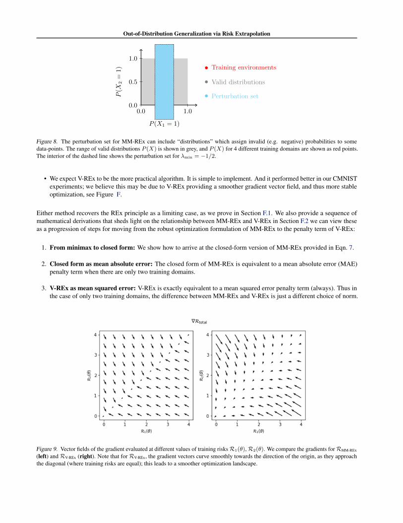
Figure 8. The perturbation set for MM-REx can include “distributions” which assign invalid (e.g. negative) probabilities to somedata-points. The range of valid distributions P (X) is shown in grey, and P (X) for 4 different training domains are shown as red points.The interior of the dashed line shows the perturbation set for λmin = −1/2.

• We expect V-REx to be the more practical algorithm. It is simple to implement. And it performed better in our CMNISTexperiments; we believe this may be due to V-REx providing a smoother gradient vector field, and thus more stableoptimization, see Figure F.

Either method recovers the REx principle as a limiting case, as we prove in Section F.1. We also provide a sequence ofmathematical derivations that sheds light on the relationship between MM-REx and V-REx in Section F.2 we can view theseas a progression of steps for moving from the robust optimization formulation of MM-REx to the penalty term of V-REx:

1. From minimax to closed form: We show how to arrive at the closed-form version of MM-REx provided in Eqn. 7.

2. Closed form as mean absolute error: The closed form of MM-REx is equivalent to a mean absolute error (MAE)penalty term when there are only two training domains.

3. V-REx as mean squared error: V-REx is exactly equivalent to a mean squared error penalty term (always). Thus inthe case of only two training domains, the difference between MM-REx and V-REx is just a different choice of norm.

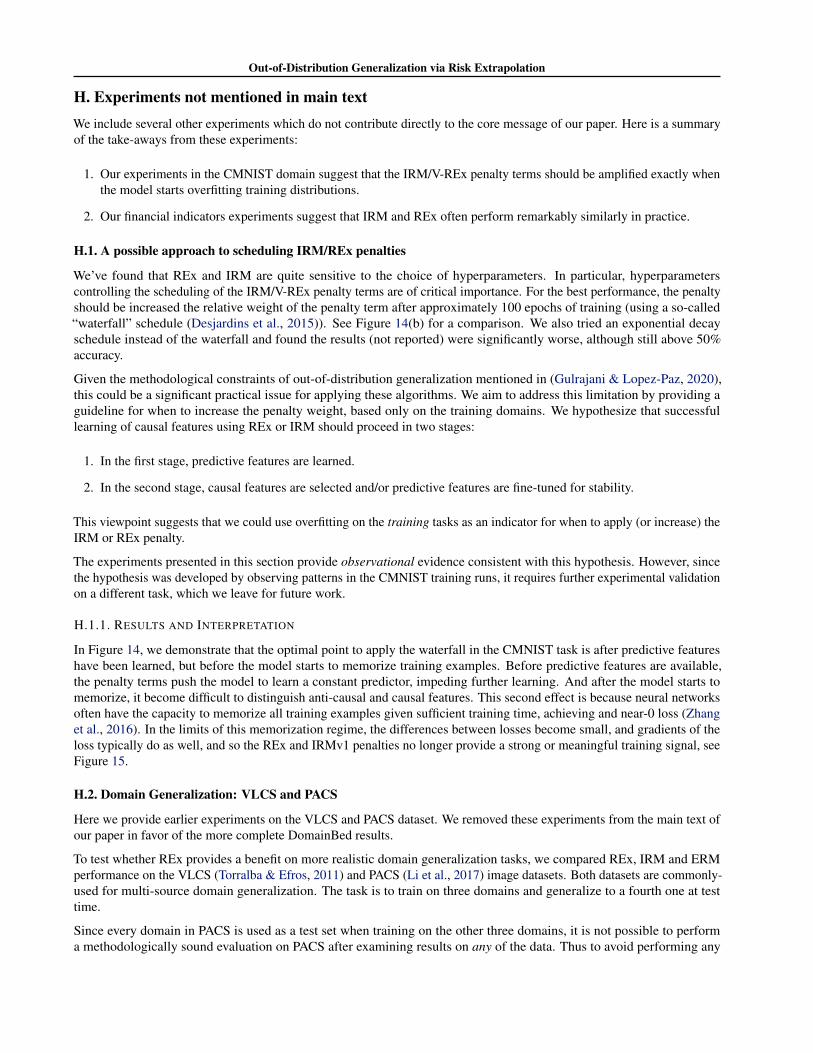
Figure 9. Vector fields of the gradient evaluated at different values of training risksR1(θ),R2(θ). We compare the gradients forRMM-REx

(left) andRV-REx (right). Note that forRV-REx, the gradient vectors curve smoothly towards the direction of the origin, as they approachthe diagonal (where training risks are equal); this leads to a smoother optimization landscape.


F.1. V-REx and MM-REx enforce the REx principle in the limit

We prove that both MM-REx and V-REx recover the constraint of perfect equality between risks in the limit of λmin → −∞or β →∞, respectively. For both proofs, we assume all training risks are finite.

Proposition 1. The MM-REx risk of predictor fθ,RMM−REx(θ)→∞ as λmin → −∞ unlessRd = Re for all trainingdomains d, e.

Proof. Suppose the risk is not equal across domains, and let the largest difference between any two training risks beε > 0. Then RMM−REx(θ) = (1 − mλmin) maxeRe(θ) + λmin

∑mi=1Ri(θ) = maxeRe(θ) − mλmin maxeRe(θ) +

λmin

∑mi=1Ri(θ) ≥ maxeRe(θ)− λminε, with the inequality resulting from matching up the m copies of λmin maxeRe

with the terms in the sum and noticing that each pair has a non-negative value (since Ri −maxeRe is non-positive andλmin is negative), and at least one pair has the value −λminε. Thus sending λ→ −∞ sends this lower bound onRMM−REx

to∞ and henceRMM−REx →∞ as well.

Proposition 2. The V-REx risk of predictor fθ, RV−REx(θ) → ∞ as β → ∞ unless Rd = Re for all training domainsd, e.

Proof. Again, let ε > 0 be the largest difference in training risks, and let µ be the mean of the training risks. Then there mustexist an e such that |Re − µ| ≥ ε/2. And thus V ari(Ri(θ)) =

∑i(Ri − µ)2 ≥ (ε/2)2, since all other terms in the sum are

non-negative. Since ε > 0 by assumption, the penalty term is positive and thusRV−REx(θ).=∑iRi(θ) + βV ari(Ri(θ))

goes to infinity as β →∞.

F.2. Connecting MM-REx to V-REx

F.2.1. CLOSED FORM SOLUTIONS TO RISK INTERPOLATION AND MINIMAX-REX

Here, we show that risk interpolation is equivalent to the robust optimization objective of Eqn. 5. Without loss of generality,let R1 be the largest risk, so Re ≤ R1, for all e. Thus we can express Re = R1 − de for some non-negative de, withd1 = 0 ≥ de for all e. And thus we can write the weighted sum of Eqn. 7 as:

RMM(θ).= max

Σeλe=1λe≥λmin

m∑e=1

λeRe(θ) (12)

= maxΣeλe=1λe≥λmin

m∑e=1

λe(R1(θ)− de) (13)

= R1(θ) + maxΣeλe=2λe≥λmin

m∑e=1

−λe(de) (14)

(15)

Now, since de are non-negative, −de is non-positive, and the maximal value of this sum is achieved when λe = λmin for alle ≥ 2, which also implies that λ1 = 1− (m− 1)λmin. This yields the closed form solution provided in Eqn. 7. The specialcase of Risk Interpolation, where λmin = 0, yields Eqn. 5.

F.2.2. MINIMAX-REX AND MEAN ABSOLUTE ERROR REX

In the case of only two training risks, MM-REx is equivalent to using a penalty on the mean absolute error (MAE) betweentraining risks. However, penalizing the pairwise absolute errors is not equivalent when there are m > 2 training risks, as weshow below. Without loss of generality, assume thatR1 < R2 < ... < Rm. Then (1/2 of) theRMAE penalty term is:


∑i

∑j≤i

(Ri −Rj) = mRm −∑j≤m

Rj + (m− 1)Rm−1 −∑

j≤m−1

Rj . . . (16)

=∑j

jRj −∑j

∑i≤j

Ri (17)

=∑j

jRj −∑j

(m− j + 1)Rj (18)

=∑j

(2j −m− 1)Rj (19)

For m = 2, we have 1/2RMAE = (2 ∗ 1− 2− 1)R1 + (2 ∗ 2− 2− 1)R2 = R2 −R1. Now, adding this penalty term withsome coefficient βMAE to the ERM term yields:

RMAE.= R1 +R2 + βMAE(R2 −R1) = (1− βMAE)R1 + (1 + βMAE)R2 (20)

(21)

We wish to show that this is equal toRMM for an appropriate choice of learning rate γMAE and hyperparameter βMAE. Stillassuming thatR1 < R2, we have that:

RMM.= (1− λmin)R2 + λminR1 (22)

Choosing γMAE = 1/2γMM is equivalent to multiplyingRMM by 2, yielding:

2RMM.= 2(1− λmin)R2 + 2λminR1 (23)

Now, in order forRMAE = 2RMM, we need that:

2− 2λmin = 1 + βMAE (24)2λmin = 1− βMAE (25)

(26)

And this holds whenever βMAE = 1− 2λmin. When m > 2, however, these are not equivalent, since RMM puts equal weighton all but the highest risk, whereasRMAE assigns a different weight to each risk.

F.2.3. PENALIZING PAIRWISE MEAN SQUARED ERROR (MSE) YIELDS V-REX

The V-REx penalty (Eqn. 8) is equivalent to the average pairwise mean squared error between all training risks (up to aconstant factor of 2). Recall thatRi denotes the risk on domain i. We have:

1

2n2

∑i

∑j

(Ri −Rj)2=

1

2n2

∑i

∑j

(R2i +R2

j − 2RiRj)

(27)

=1

2n

∑i

R2i +

1

2n

∑j

R2j −

1

n2

∑i

∑j

RiRj (28)

=1

n

∑i

R2i −

(1

n

∑i

Ri

)2

(29)

= Var(R) . (30)

G. Further results and details for experiments mentioned in main textG.1. CMNIST with covariate shift

Here we present the following additional results:


1. Figure 1 of the main text with additional results using MM-REx, see G.1. These results used the “default” parametersfrom the code of Arjovsky et al. (2019).

2. A plot with results on these same tasks after performing a random search over hyperparameter values similar to thatperformed by Arjovsky et al. (2019).

3. A plot with the percentage of the randomly sampled hyperparameter combinations that have satisfactory (> 50%)accuracy, which we count as “success” since this is better than random chance performance.

These results show that REx is able to handle greater covariate shift than IRM, given appropriate hyperparameters.Furthermore, when appropriately tuned, REx can outperform IRM in situations with covariate shift. The lower success rateof REx for high values of p is because it produces degenerate results (where training accuracy is less than test accuracy)more often.

The hyperparameter search consisted of a uniformly random search of 340 samples over the following intervals of thehyperparameters:

1. HiddenDim = [2**7, 2**12]

2. L2RegularizerWeight = [10**-2, 10**-4]

3. Lr = [10**-2.8, 10**-4.3]

4. PenaltyAnnealIters = [50, 250]

5. PenaltyWeight = [10**2, 10**6]

6. Steps = [201, 601]

0.00.10.20.30.40.5p = P(shape(x) {0,1,2,3,4})

0.2

0.3

0.4

0.5

0.6

Test

Acc

urac

y

Random GuessingV-RExIRMMM-REx

0.00.10.20.30.40.5p = P(shape(x) {1,2} {6,7})

0.2

0.3

0.4

0.5

0.6

0.7

Test

Acc

urac

y

Random GuessingRExIRMMM-REx

0.00.10.20.30.40.5p = P(R1|Red) = P(G1|Green)

0.1

0.2

0.3

0.4

0.5

0.6

Test

Acc

urac

y

Random GuessingRExIRMMM-REx

Figure 10. This is Figure 3.2 of main text with additional results using MM-REx. For each covariate shift variant (class imbalance, digitimbalance, and color imbalance from left to right as described in "CMNIST with covariate shift" subsubsection of Section 4.1 in maintext) of CMNIST, the standard error (the vertical bars in plots) is higher for MM-REx than for V-REx.

0.00.10.20.30.4p = P(shape(x) {0,1,2,3,4})

0.3

0.4

0.5

0.6

0.7

Test

Acc

urac

y

Random GuessingRExIRM

0.00.10.20.30.4p = P(shape(x) {1,2} {6,7})

0.4

0.5

0.6

0.7

Test

Acc

urac

y


0.00.10.20.30.4p = P(R1|Red) = P(G1|Green)

0.3

0.4

0.5

0.6

0.7

Test

Acc

urac

y


Figure 11. This is Figure 3.2 of main text (class imbalance, digit imbalance, and color imbalance from left to right as described in"CMNIST with covariate shift" subsubsection of Section 4.1 in main text), but with hyperparameters of REx and IRM each tuned toperform as well as possible for each value of p for each covariate shift type.


0.00.10.20.30.4p = P(shape(x) {0,1,2,3,4})

0

10

20

30

perc

ent_

of_r

uns_

that

_are

_sat

isfac

tory

RExIRM

0.00.10.20.30.4p = P(shape(x) {1,2} {6,7})

0

10

20

30

perc

ent_

of_r

uns_

that

_are

_sat

isfac

tory

RExIRM

0.00.10.20.30.4p = P(R1|Red) = P(G1|Green)

0

10

20

30

perc

ent_

of_r

uns_

that

_are

_sat

isfac

tory

RExIRM

Figure 12. This also corresponds to class imbalance, digit imbalance, and color imbalance from left to right as described in "CMNISTwith covariate shift" subsubsection of Section 4.1 in main text; but now the y-axis refers to what percentage of the randomly sampledhyperparameter combinations we deemed to to be satisfactory. We define satisfactory as simultaneously being better than random guessingand having train accuracy greater than test accuracy. For p less than .5, a larger percentage of hyperparameter combinations are oftensatisfactory for REx than for IRM; for p greater than .5, a larger percentage of hyperparameter combinations are often satisfactory forIRM than for REx because train accuracy is greater than test accuracy for more hyperparameter combinations for IRM. We stipulate thattrain accuracy must be greater than test accuracy because test accuracy being greater than train accuracy usually means the model haslearned a degenerate prediction rule such as "not color".

G.2. SEMs from “Invariant Risk Minimization”

Here we present experiments on the (linear) structural equation model (SEM) tasks introduced by Arjovsky et al. (2019).Arjovsky et al. (2019) construct several varieties of SEM where the task is to predict targets Y from inputs X1, X2, whereX1 are (non-anti-causal) causes of Y , and X2 are (anti-causal) effects of Y . We refer the reader to Section 5.1 and Figure 3of Arjovsky et al. (2019) for more details. We use the same experimental settings as Arjovsky et al. (2019) (except we onlyrun 7 trials), and report results in Table 5.

These experiments include several variants of a simple SEM, given by:

X1 = N1

Y = W1→YX1 +NY

X2 = WY→2Y +N2

Where N1, NY , N2 are all sampled i.i.d. from normal distributions. The variance of these distributions may vary acrossdomains.

While REx achieves good performance in the domain-homoskedastic case, it performs poorly in the domain-heteroskedastic case, where the amount of intrinsic noise, σ2

y in the target changes across domains.10 Intuitively, this isbecause the irreducible error varies across domains in these tasks, meaning that the risk will be larger on some domains thanothers, even if the model’s predictions match the expectation E(Y |Pa(Y )). We tried using a “baseline” (see Eqn. 5) ofre = V ar(Ye) (Meinshausen et al., 2015) to account for the different noise levels in Y , but this did not work.

We include a mathematical analysis of the simple SEM given above in order to better understand why REx succeeds in thedomain-homoskedastic, but not the domain-heteroskedastic case. Assuming that Y,X1, X2 are scalars, this SEM becomes

X1 = N1

Y = w1→yN1 +NY

X2 = wy→2w1→yN1 + wy→2NY +N2

We consider learning a model Y = αX1 + βX2. Then the residual is:

Y − Y = (α+ w1→y(βwy→2 − 1))N1 + (βwy→2 − 1)NY + βN2

Since all random variables have zero mean, the MSE loss is the variance of the residual. Using the fact that the noiseN1, NY , N2 are independent, this equals:

E[(Y − Y )2] = (α+ w1→y(βwy→2 − 1))2σ21 + (βwy→2 − 1)2σ2

Y + β2σ22

10See Footnote 6.


FOU(c) FOU(nc) FOS(c) FOS(nc)

IRM 0.001±0.000 0.001±0.000 0.001±0.000 0.000±0.000REx, re = 0 0.001±0.000 0.008±0.002 0.007±0.002 0.000±0.000REx, re = V(Ye) 0.816±0.149 1.417±0.442 0.919±0.091 0.000±0.000

POU(c) POU(nc) POS(c) POS(nc)


FEU(c) FEU(nc) FES(c) FES(nc)


PEU(c) PEU(nc) PES(c) PES(nc)


Table 5. Average mean-squared error between true and estimated weights on causal (X1) and non-causal (X2) variables. Top 2: Whenthe level of noise in the anti-causal features varies across domains, REx performs well (FOU, FOS, POU, POS). Bottom 2: When thelevel of noise in the targets varies instead, REx performs poorly (FEU, FES, PEU, PES). Using the baselines re = V(Y ) does not solvethe problem, and indeed, hurts performance on the homoskedastic domains.

Thus when (only) σ2 changes, the only way to keep the loss unchanged is to set the coefficient in front of σ2 to 0, meaningβ = 0. By minimizing the loss, we then recover α = w1→y; i.e. in the domain-homoskedastic setting, the loss equalityconstraint of REx yields the causal model. On the other hand, if (only) σY changes, then REx enforces β = 1/wy→2, whichthen induces α = 0, recovering the anticausal model.

While REx (like ICP (Peters et al., 2016)) assumes the mechanism for Y is fixed across domains (meaning P (Y |Pa(Y )) isindependent of the domain, e), IRM makes the somewhat weaker assumption that E(Y |Pa(Y )) is independent of domain.While it is plausible that an appropriately designed variant of REx could work under this weaker assumption, we believeforbidding interventions on Y is not overly restrictive, and such an extension for future work.

G.3. Reinforcement Learning Experiments

Here we provide details and further results on the experiments in Section 4.1. We take tasks from the Deepmind ControlSuite (Tassa et al., 2018) and modify the original state, s, to produce observation, o = (s + ε, ηs′) including noise ε andspurious features ηs′, where s′ contains 1 or 2 dimensions of s. The scaling factor takes values η = 1/2/3 for the two trainingand test domains, respectively. The agent takes o as input and learns a representation using Soft Actor-Critic (Haarnojaet al., 2018) and an auxiliary reward predictor, which is trained to predict the next 3 rewards conditioned on the next 3actions. Since the spurious features are copied from the state before the noise is added, they are more informative for thereward prediction task, but they do not have an invariant relationship with the reward because of the domain-dependent η.

The hyperparameters used for training Soft Actor-Critic can be found in Table 6. We used cartpole_swingup as adevelopment task to tune the hyperparameters of penalty weight (chosen from [0.01, 0.1, 1, 10]) and number of iterationsbefore the penalty is turned up (chosen from [5000, 10000, 20000]), both for REx and IRM. The plots with the hyperparametersweep are in Figure 13.


0 50000 100000 150000 200000 250000 300000step

100

120

140

160

180

200

220

240

260

Episo

de R

ewar

dcartpole_swingup_iters5000_penalty0.01

rrex_erm_2envs_iters5000_penalty0.01_criticbackprop_rewardlossrrex_irm_2envs_iters5000_penalty0.01_criticbackprop_rewardlossrrex_rex_2envs_iters5000_penalty0.01_criticbackprop_rewardloss

0 50000 100000 150000 200000 250000step

100

120

140

160

180

200

220

240

260

Episo

de R

ewar

d

cartpole_swingup_iters5000_penalty0.1


0 50000 100000 150000 200000 250000 300000 350000 400000 450000step

75

100

125

150

175

200

225

250

275

Episo

de R

ewar

d

cartpole_swingup_iters5000_penalty1

rrex_erm_2envs_iters5000_penalty1_criticbackprop_rewardlossrrex_irm_2envs_iters5000_penalty1_criticbackprop_rewardlossrrex_rex_2envs_iters5000_penalty1_criticbackprop_rewardloss

0 100000 200000 300000 400000step

80

100

120

140

160

180

200

220

240

260

Episo

de R

ewar

d



0 50000 100000 150000 200000 250000 300000 350000 400000step

100

150

200

250

300

350

Episo

de R

ewar

d



0 50000 100000 150000 200000 250000 300000 350000step

100

120

140

160

180

200

220

240

260

280

Episo

de R

ewar

d



0 50000 100000 150000 200000 250000 300000 350000 400000step

120

140

160

180

200

220

240

260

280

Episo

de R

ewar

d



0 100000 200000 300000 400000step

100

120

140

160

180

200

220

240

260

Episo

de R

ewar

d



0 100000 200000 300000 400000 500000 600000 700000 800000step

100

150

200

250

300

350

Episo

de R

ewar

d



0 50000 100000 150000 200000 250000 300000step

80

100

120

140

160

180

200

220

240

Episo

de R

ewar

d



0 50000 100000 150000 200000 250000 300000step

100

125

150

175

200

225

250

275

300

Episo

de R

ewar

d



0 50000 100000 150000 200000 250000 300000step

100

125

150

175

200

225

250

275

300

Episo

de R

ewar

d



Figure 13. Hyperparameter sweep for IRM and REx on cartpole_swingup. Green, blue, and orange curves correspond to REx,ERM, and IRM, respectively. The subfigure titles state the penalty strength (“penalty”) and after how many iterations the penalty strengthwas increased (“iters”). We chose a penalty factor of 1 and 10k iterations.

Parameter name ValueReplay buffer capacity 1000000Batch size 1024Discount γ 0.99Optimizer AdamCritic learning rate 10−5

Critic target update frequency 2Critic Q-function soft-update rate τQ 0.005Critic encoder soft-update rate τenc 0.005Actor learning rate 10−5

Actor update frequency 2Actor log stddev bounds [−5, 2]Encoder learning rate 10−5

Decoder learning rate 10−5

Decoder weight decay 10−7

L1 regularization weight 10−5

Temperature learning rate 10−4

Temperature Adam’s β1 0.9Init temperature 0.1

Table 6. A complete overview of hyperparameters used for reinforcement learning experiments.


H. Experiments not mentioned in main textWe include several other experiments which do not contribute directly to the core message of our paper. Here is a summaryof the take-aways from these experiments:

1. Our experiments in the CMNIST domain suggest that the IRM/V-REx penalty terms should be amplified exactly whenthe model starts overfitting training distributions.

2. Our financial indicators experiments suggest that IRM and REx often perform remarkably similarly in practice.

H.1. A possible approach to scheduling IRM/REx penalties

We’ve found that REx and IRM are quite sensitive to the choice of hyperparameters. In particular, hyperparameterscontrolling the scheduling of the IRM/V-REx penalty terms are of critical importance. For the best performance, the penaltyshould be increased the relative weight of the penalty term after approximately 100 epochs of training (using a so-called“waterfall” schedule (Desjardins et al., 2015)). See Figure 14(b) for a comparison. We also tried an exponential decayschedule instead of the waterfall and found the results (not reported) were significantly worse, although still above 50%accuracy.

Given the methodological constraints of out-of-distribution generalization mentioned in (Gulrajani & Lopez-Paz, 2020),this could be a significant practical issue for applying these algorithms. We aim to address this limitation by providing aguideline for when to increase the penalty weight, based only on the training domains. We hypothesize that successfullearning of causal features using REx or IRM should proceed in two stages:

1. In the first stage, predictive features are learned.

2. In the second stage, causal features are selected and/or predictive features are fine-tuned for stability.

This viewpoint suggests that we could use overfitting on the training tasks as an indicator for when to apply (or increase) theIRM or REx penalty.

The experiments presented in this section provide observational evidence consistent with this hypothesis. However, sincethe hypothesis was developed by observing patterns in the CMNIST training runs, it requires further experimental validationon a different task, which we leave for future work.

H.1.1. RESULTS AND INTERPRETATION

In Figure 14, we demonstrate that the optimal point to apply the waterfall in the CMNIST task is after predictive featureshave been learned, but before the model starts to memorize training examples. Before predictive features are available,the penalty terms push the model to learn a constant predictor, impeding further learning. And after the model starts tomemorize, it become difficult to distinguish anti-causal and causal features. This second effect is because neural networksoften have the capacity to memorize all training examples given sufficient training time, achieving and near-0 loss (Zhanget al., 2016). In the limits of this memorization regime, the differences between losses become small, and gradients of theloss typically do as well, and so the REx and IRMv1 penalties no longer provide a strong or meaningful training signal, seeFigure 15.

H.2. Domain Generalization: VLCS and PACS

Here we provide earlier experiments on the VLCS and PACS dataset. We removed these experiments from the main text ofour paper in favor of the more complete DomainBed results.

To test whether REx provides a benefit on more realistic domain generalization tasks, we compared REx, IRM and ERMperformance on the VLCS (Torralba & Efros, 2011) and PACS (Li et al., 2017) image datasets. Both datasets are commonly-used for multi-source domain generalization. The task is to train on three domains and generalize to a fourth one at testtime.

Since every domain in PACS is used as a test set when training on the other three domains, it is not possible to performa methodologically sound evaluation on PACS after examining results on any of the data. Thus to avoid performing any


0 100 200 300 400

0.50

0.55

0.60

0.65

0.70

accu

racy

(%) IRM

REx

0 100 200 300 4000.00

0.02

0.04

0.06

accu

racy

(%) train generalization gap (%)

overfitting

0 100 200 300 400epoch

0.2

0.4

0.6

0.8

accu

racy

(%)

testtraingrayscale

Figure 14. Stability penalties should be applied around when traditional overfitting begins, to ensure that the model has learned predictivefeatures, and that penalties still give meaningful training signals. Top: Test accuracy as a function of epoch at which penalty term weightis increased (learning rate is simultaneously decreased proportionally). Choosing this hyperparameter correctly is essential for goodperformance. Middle: Generalization gap on a validation set with 85% correlation between color and label (the same as the averagetraining correlation). The best test accuracy is achieved by increasing the penalty when the generalization gap begins to increase. Theincrease clearly indicates memorization because color and shape are only 85%/75% correlated with the label, and so cannot be usedto make predictions with higher than 85% accuracy. Bottom: Accuracy on training/test sets, as well as an auxilliary grayscale set.Training/test performance reach 85%/15% after a few epochs of training, but grayscale performance improves, showing that meaningfulfeatures are still being learned.

tuning on test distributions, we use VLCS to tune hyperparameters and then apply these exact same settings to PACS andreport the final average over 10 runs on each domain.

We use the same architecture, training procedure and data augmentation strategy as the (formerly) state-of-the-art JigsawPuzzle approach (Carlucci et al., 2019) (except with IRM or V-REx intead of JigSaw as auxilliary loss) for all three methods.As runs are very noisy, we ran each experiment 10 times, and report average test accuracies extracted at the time of the


0 5000 10000 15000 20000 25000epoch

10 16

10 13

10 10

10 7

10 4

10 1

102

loss

train_nllirmv1_penaltyrex_penalty

Figure 15. Given sufficient training time, empirical risk minimization (ERM) minimizes both REx and IRMv1 penalty terms on ColoredMNIST (without including either term in the loss function). This is because the model (a deep network) has sufficient capacity to fit thetraining sets almost perfectly. This prevents these penalties from having the intended effect, once the model has started to overfit. They-axis is in log-scale.

highest validation accuracy on each run. Results on PACS are in Table 8. On PACS we found that REx outperforms IRMand IRM outperforms ERM on average, while all are worse than the state-of-the-art Jigsaw method.

We use all hyperparameters from the original Jigsaw codebase.11 We use Imagenet pre-trained AlexNet features and chosebatch-size, learning rate, as well as penalty weights based on performance on the VLCS dataset where test performanceon the holdout domain was used for the set of parameters producing the highest validation accuracy. The best performingparameters on VLCS were then applied to the PACS dataset without further changes. We searched over batch-sizes in{128, 384}, over penalty strengths in {0.0001, 0.001, 0.01, 0.1, 1, 10}, learning rates in {0.001, 0.01} and used averageperformance over all 4 VLCS domains to pick the best performing hyperparameters. Table 7 shows results on VLCS withthe best performing hyperparameters.

The final parameters for all methods on PACS were a batch size of 384 with 30 epochs of training with Adam, using alearning rate of 0.001, and multiplying it by 0.1 after 24 epochs (this step schedule was taken from the Jigsaw repo).Thepenalty weight chosen for Jigsaw was 0.9; for IRM and REx it was 0.1.We used the same data-augmentation pipeline as theoriginal Jigsaw code for ERM, IRM, Jigsaw and REx to allow for a fair comparison.

VLCS CALTECH SUN PASCAL LABELME Average

REx (ours) 96.72 63.68 72.41 60.40 73.30IRM 95.99 62.85 71.71 59.61 72.54ERM 94.76 61.92 69.03 60.55 71.56Jigsaw (SOTA) 96.46 63.84 70.49 60.06 72.71

Table 7. Accuracy (percent) of different methods on the VLCS task. Results are test accuracy at the time of the highest validationaccuracy, averaged over 10 runs. On VLCS REx outperforms all other methods. Numbers are shown in strike-through because we selectedour hyperparameters based on highest test set performance; the goal of this experiment was to find suitable hyperparameters for the PACSexperiment.

11https://github.com/fmcarlucci/JigenDG

https://github.com/fmcarlucci/JigenDG


PACS Art Painting Cartoon Sketch Photo Average

REx (ours) 66.27±0.46 68.8±0.28 59.57±0.78 89.60±0.12 71.07IRM 66.46±0.31 68.60±0.40 58.66±0.73 89.94±0.13 70.91ERM 66.01±0.22 68.62±0.36 58.38±0.60 89.40±0.18 70.60

Jigsaw (SOTA) 66.96±0.39 66.67±0.41 61.27±0.73 89.54±0.19 71.11

Table 8. Accuracy (percent) of different methods on the PACS task. Results are test accuracy at the time of the highest validation accuracy,averaged over 10 runs. REx outperforms ERM on average, and performs similar to IRM and Jigsaw (the state-of-the-art).

2014

2015

2016

2017

2018

Task

Training envs.

2014

2015

2016

2017

2018

Test IRM

2014

2015

2016

2017

2018

Test REx

0.10

0.05

0.00

0.05

0.10

Perfo

rman

ce re

lativ

e to

ERM

Figure 16. Financial indicators tasks. The left panel indicates the set of training domains; the middle and right panels show the testaccuracy on the respective domains relative to ERM (a black dot corresponds to a training domain; a colored patch indicates the testaccuracy on the respective domain.)

H.3. Financial indicators

We find that IRM and REx seem to perform similarly across different splits of the data in a prediction task using financialdata. The dataset is split into five years, 2014–18, containing 37 publicly reported financial indicators of several thousandpublicly listed companies each. The task is to predict if a company’s value will increase or decrease in the following year(see Appendix for dataset details.) We consider each year a different domain, and create 20 different tasks by selectingall possible combinations of domains where three domains represent the training sets, one domain the validation set, andanother one the test set. We train an MLP using the validation set to determine an early stopping point, with β = 104. Theper-task results summarized in fig. 16 indicate substantial differences between ERM and IRM, and ERM and REx. Thepredictions produced by IRM and REx, however, only differ insignificantly, highlighting the similarity of IRM and REx.While performance on specific tasks differs significantly between ERM and IRM/REx, performance averaged over tasks isnot significantly different.

H.3.1. EXPERIMENT DETAILS

We use v1 of the dataset published on 12 and prepare the data as described in.13 We further remove all the variables that arenot shared across all 5 years, leaving us with 37 features, and whiten the data through centering and normalizing by thestandard deviation.

On each subtask, we train an MLP with two hidden layers of size 128 with tanh activations and dropout (p=0.5) after eachlayer. We optimize the binary cross-entropy loss using Adam (learning rate 0.001, β1 = 0.9, β2 = 0.999, ε = 10−8), and anL2 penalty (weight 0.001). In the IRM/REx experiments, the respective penalty is added to the loss (β = 1) and the originalloss is scaled by a factor 10−4 after 1000 iterations. Experiments are run for a maximum of 9000 training iterations withearly stopping based on the validation performance. All results are averaged over 3 trials. The overall performance of thedifferent models, averaged over all tasks, is summarized in Tab. 9. The difference in average performance between ERM,IRM, and REx is not statistically significant, as the error bars are very large.

12https://www.kaggle.com/cnic92/200-financial-indicators-of-us-stocks-2014201813https://www.kaggle.com/cnic92/explore-and-clean-financial-indicators-dataset

https://www.kaggle.com/cnic92/200-financial-indicators-of-us-stocks-20142018

https://www.kaggle.com/cnic92/explore-and-clean-financial-indicators-dataset


Overall accuracy Min acc. Max acc.

ERM 54.6± 4.6 47.6 66.2IRM 55.3± 5.9 45.9 67.5REx 55.5± 6.0 47.2 68.0

Table 9. Test accuracy of models trained on the financial domain dataset, averaged over all 20 tasks, as well as min./max. accuracy acrossthe tasks.

I. Overview of other topics related to OOD generalizationDomain adaptation (Ben-David et al., 2010a) shares the goal of generalizing to new distributions at test time, but allowssome access to the test distribution. A common approach is to make different domains have a similar distribution of features(Pan et al., 2010). A popular deep learning method for doing so is Adversarial Domain Adaptation (ADA) (Ganin et al.,2016; Tzeng et al., 2017; Long et al., 2018; Li et al., 2018), which seeks a “invariant representation” of the inputs, i.e. onewhose distribution is domain-independent. Recent works have identified fundamental shortcomings with this approach,however (Zhao et al., 2019; Johansson et al., 2019; Arjovsky et al., 2019; Wu et al., 2020).

Complementary to the goal of domain generalization is out-of-distribution detection (Hendrycks & Gimpel, 2016;Hendrycks et al., 2018), where the goal is to recognize examples as belonging to a new domain. Three common deeplearning techniques that can improve OOD generalization are adversarial training (Goodfellow et al., 2014; Hendrycks& Dietterich, 2019), self-supervised learning (van den Oord et al., 2018; Hjelm et al., 2018; Hendrycks et al., 2019b;Albuquerque et al., 2020) and data augmentation (Krizhevsky et al., 2012; Zhang et al., 2017; Cubuk et al., 2018; Shorten& Khoshgoftaar, 2019; Hendrycks et al., 2019a; Carlucci et al., 2019). These methods can also been combined effectively invarious ways (Tian et al., 2019; Bachman et al., 2019; Gowal et al., 2019). Data augmentation and self-supervised learningmethods typically use prior knowledge such as 2D image structure. Several recent works also use prior knowledge todesign augmentation strategies for invariance to superficial features that may be spuriously correlated with labels in objectrecognition tasks (He et al., 2019; Wang et al., 2019; Gowal et al., 2019; Ilse et al., 2020). In contrast, REx can discoverwhich features have invariant relationships with the label without such prior knowledge.

Date post:	27-Dec-2021
Category:	Documents
Upload:	others
View:	1 times
Download:	0 times

Out-of-Distribution Generalization via Risk Extrapolation

Documents