VALUE RELEVANT ASSET MEASUREMENT AND ASSET USE: EVIDENCE

FROM INTERNATIONAL ACCOUNTING STANDARD 41

by

Adrienna Alys Huffman

A dissertation submitted to the faculty of The University of Utah

in partial fulfillment of the requirements for the degree of

Doctor of Philosophy

in

Business Administration

David Eccles School of Business

The University of Utah

August 2014

All rights reserved

INFORMATION TO ALL USERSThe quality of this reproduction is dependent upon the quality of the copy submitted.

In the unlikely event that the author did not send a complete manuscriptand there are missing pages, these will be noted. Also, if material had to be removed,

a note will indicate the deletion.

Microform Edition © ProQuest LLC.All rights reserved. This work is protected against

unauthorized copying under Title 17, United States Code

ProQuest LLC.789 East Eisenhower Parkway

P.O. Box 1346Ann Arbor, MI 48106 - 1346

UMI 3640139Published by ProQuest LLC (2014). Copyright in the Dissertation held by the Author.

UMI Number: 3640139

Copyright © Adrienna Alys Huffman 2014

All Rights Reserved

T h e U n i v e r s i t y o f U t a h G r a d u a t e S c h o o l

STATEMENT OF DISSERTATION APPROVAL

The dissertation of Adrienna Alys Huffman

has been approved by the following supervisory committee members:

Christine A. Botosan , Chair 5/22/2014

Date Approved

Melissa Lewis , Member 5/22/2014

Date Approved

Marlene Plumlee , Member 5/22/2014

Date Approved

James Schallheim , Member 5/22/2014

Date Approved

Haimanti Bhattacharya , Member 5/22/2014

Date Approved

and by William Hesterly , Associate

Dean of David Eccles School of Business

and by David B. Kieda, Dean of The Graduate School.

ABSTRACT

This dissertation is the first to empirically test an asset measurement framework

that links asset measurement to asset use. Specifically, I examine whether fair value

applied to in-exchange assets and historical cost applied to in-use assets (i.e.

measurement consistent with asset use) produces incrementally more value relevant

information than when historical cost is applied to in-exchange assets and fair value is

applied to in-use assets (i.e. measurement inconsistent with asset use). I test the

framework on a sample of 182 international firms from 33 different countries that adopt

International Accounting Standard (IAS) 41. IAS 41 prescribes fair value measurement

for biological assets, a class of assets previously classified as property, plant, and

equipment and measured at historical cost. I find that book value and earnings

information is more value relevant when measurement is consistent with asset use as

compared to when asset measurement is not linked to asset use. At present, the

Conceptual Framework provides little guidance on asset measurement and when certain

measurement bases should be used, resulting in inconsistencies across measurement

standards. My findings provide evidence supporting a framework for asset measurement,

which links asset measurement to asset use. These findings should be of interest to

standard setters’ and others interested in conceptually based asset measurement.

To my parents, Boyd and Carlotta, without whom none of this would be possible. Thank you for your unending love and support; you are truly my biggest fans.

vi

TABLE OF CONTENTS

ABSTRACT ...…………….……………………………………………………………...iii

LIST OF TABLES...…………………………………………………………………….. vii

LIST OF FIGURES………..……………………………………………………………viii

ACKNOWLEDGMENTS....……………………………………...……………………...ix

CHAPTERS

1. INTRODUCTION……..………………………………………………....................... 1

2. LITERATURE REVIEW………………...……………………………………...........7

2.1 Asset Measurement Frameworks………………………..……………………......7 2.2 Research on Fair Value Accounting…………………………………………........9 2.3 Research on Historical Cost Accounting.............................................................. .12

3. MOTIVATION AND HYPOTHESES…………………………..…………………..15 3.1 IAS 41 Background……………………………………….…………………..….15 3.2 Main Hypothesis…………………………………...………………………….... 20

4. RESEARCH DESIGN……………………………………………………..………... 23

4.1 Consistent and Inconsistent Measurement Samples.…………………………… 25 4.2 Interpretation of the Results………………………..…………………………… 26 4.3 Price and Return Tests…………..………………….…………………………… 27 4.4 Mechanical Forecast Models……………………………………………....……. 30

5. SAMPLE SELECTION AND DESCRIPTIVE STATISTICS..…………….......... 35

5.1 Sample Identification and Data Sources…………………………………………35 5.2 Descriptive Statistics…………………..…………………………………………36

6. RESULTS…………………....…………………………………………………........47

6.1 Cross-Sectional Results..……………...................................................................47

vi

6.1.1 Price and Return Results……..….…………………………………………47 6.1.2 Operating Cash Flows and Operating Income Results……...……............. 49

6.2 Switcher Sample Results……..……………………….……………………..….. 51 6.2.1 Price and Return Results…………………………………………..……… 51 6.2.2 Operating Cash Flows and Operating Income Results……………............ 52

7. ADDITIONAL ANALYSES..…………………………………………………….... 64

7.1 Reliability Test………………………...…………………………………………64 7.2 Robustness Tests…..…………………..…………………………………………66

8. FUTURE WORK…………………………………………………………………….70

9. CONCLUSION………………………………………………………………………72

APPENDIX: VARIABLE DEFINITIONS……..…………………………………….… 74 REFERENCES……………………………………………………………………….... 76

LIST OF TABLES

5.1 Cross-Sectional Sample Composition by Country………………………………..... 42

5.2 Cross-Sectional Sample Composition by Fiscal Year………..…………………..... 43

5.3 Descriptive Statistics for the Fair Value Cross-Sectional Sample………………….. 44

5.4 Descriptive Statistics for the Historical Cost Cross-Sectional Sample….………….. 45

5.5 Descriptive Statistics for the Switcher Sample………………..…………………….. 46

6.1 Cross-Sectional Price Results………….………………………………………….. 54

6.2 Cross-Sectional Return Results …………………..……………………………..... 55

6.3 Cross-Sectional Operating Cash Flows Results …………………….…………..... 56

6.4 Cross-Sectional Future Operating Cash Flows Results …………………….……… 57

6.5 Cross-Sectional Operating Income Results…………………………………........... 58

6.6 Switcher Sample Price Results………….…………………………………….......... 59

6.7 Switcher Sample Return Results………………..…………………………….......... 60

6.8 Switcher Sample Operating Cash Flows Results …………..…………………..…... 61

6.9 Switcher Sample Future Operating Cash Flows Results ……..………………..…... 62

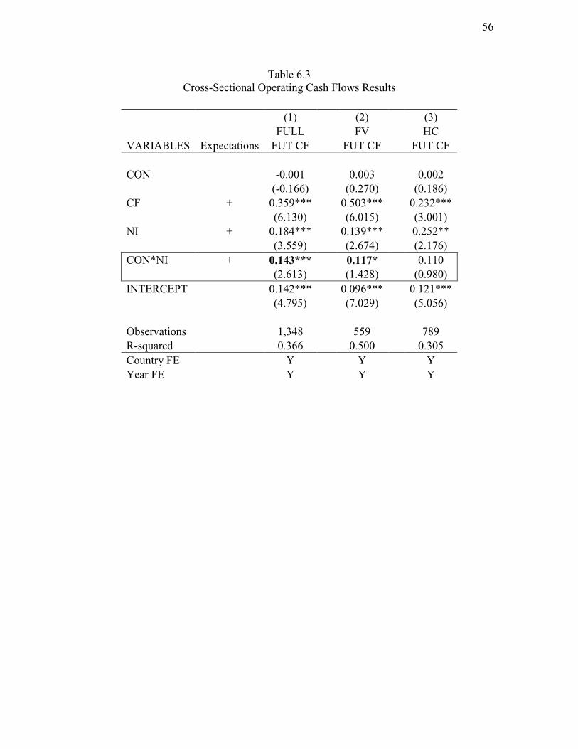
6.7 Switcher Sample Operating Income Results……………………...………………… 63

7.1 Fair Value Firm-Year Observations by Reliability Level and Value Realization….. 69

LIST OF FIGURES

3.1 Value Realization and Measurement Sample Composition for the Cross-Sectional Sample………………………………………………………………….……...........22 4.1 Switcher Sample Research Design……………..……………………………………34 5.1 Value Realization and Measurement Sample Composition for the Switcher Sample………………………………………………………..................................41

ACKNOWLEDGMENTS

I would like to thank my dissertation committee, in particular my chair Christine

Botosan, Melissa Lewis Western, Marlene Plumlee, Jim Schallheim, and Haimanti

Bhattacharya, for all of their support and invaluable feedback. I am especially grateful to

Steve Stubben for all of his excellent suggestions and help, and workshop participants

from the BYU Research Symposium, the University of Utah, the FDIC, and Tulane

University for their helpful comments.

1

CHAPTER 1

INTRODUCTION

Assets generate value via two mechanisms. In-exchange assets (e.g. cash)

generate value on a standalone basis in exchange for cash or other valuable assets, while

in-use assets (e.g. property, plant, and equipment (hereafter, PP&E)) generate value in

combination with other assets. Early accounting theorists link value relevant asset

measurement to the manner in which an asset generates value (e.g. Littleton 1935).

Specifically, this literature claims that fair value applied to in-exchange assets and

historical cost applied to in-use assets has the potential to produce incrementally more

value relevant information for investors. Nevertheless, in some cases, modern accounting

standards do not link asset measurement to the manner in which the asset generates value.

For example, International Accounting Standard (hereafter, IAS) 41 requires fair value

measurement for “biological assets,” which are living plants and animals, regardless of

whether the biological assets derive value in-use or in-exchange.

I use the adoption of IAS 41 as a setting to examine whether asset measurement

linked to asset use provides investors with incrementally more value relevant

information. The adoption of IAS 41 offers an advantageous setting to examine the

implication of linking asset measurement to asset use on the value relevance of

2

accounting information, for several reasons.

First, the extent to which assets derive value in-use or in-exchange varies across

firms for similar types of biological assets. For example, some firms own cattle for meat

production (an in-exchange asset) while other firms own cattle for dairy production (an

in-use asset). Second, the standard provides variation in asset measurement. Prior to IAS

41, firms measured their biological assets at historical cost and classified them as PP&E.

Upon adoption of the standard, some firms began measuring their biological assets at fair

value while others applied the historical cost stipulation, discussed further in Chapter 3.

Therefore, IAS 41 provides a setting where some firms measure their biological assets in

a manner consistent with their use (i.e. historical cost for in-use assets or fair value for in-

exchange assets) while others do not (i.e. historical cost for in-exchange assets or fair

value for in-use assets). In addition, before adoption of the standard, some firms measure

their biological assets consistent with their use (i.e. historical cost for in-use assets) and

then upon adoption of the standard, they do not (i.e. fair value for in-use assets). These

combinations allow for a cross-sectional and a pre- and postadoption comparison of

biological asset-groups where the asset measurement is consistent with the assets’ use,

versus when it is not for both fair value and historical cost accounting.

Third, for the firms that report their biological assets at fair value, IAS 41 is a

“true” fair value standard: the fair value of biological assets is reported on the firm’s

balance sheet, and any change in the fair value of the biological assets over the reporting

period is recognized in periodic income as an unrealized gain or loss. This mitigates

issues related to investors’ perceptions of recognized versus disclosed amounts when

firms fair value nonfinancial assets in disclosures (e.g. Beaver and Landsman 1983;

3

Ahmed et al. 2006), at discretion (e.g. Easton et al. 1993; Barth and Clinch 1998; Aboody

et al. 1999), or when provided a choice (Cairns et al. 2011; Christensen and Nikolaev

2013).

I employ a sample of 182 international firms from 33 countries that adopt IAS 41.

In a multipronged approach, I assess the value relevance of book value and earnings

information in regressions of stock price, stock returns, future operating cash flows, and

future operating income. I separate my sample into two subsamples. The first “consistent

measurement” subsample includes observations for which the measurement of biological

assets is consistent with their use (i.e. where in-exchange biological assets are measured

at fair value and in-use biological assets are measured at historical cost). The second

“inconsistent measurement” subsample includes observations for which the measurement

of biological assets is inconsistent with their use (i.e. where in-exchange biological assets

are measured at historical cost and in-use assets are measured at fair value).

My results are as follows. First, in the cross-sectional tests, I find strong support

for my hypothesis, that when measurement is linked to asset use, investors are provided

with more value relevant information. As suggested by early accounting theorists, I find

that book value and earnings information is more value relevant when asset measurement

is consistent with the manner in which the asset realizes value for the firm, relative to

when it is not. Specifically, I find that book value and earnings information is more value

relevant when in-exchange (in-use) assets are measured at fair value (historical cost) as

compared to when in-exchange (in-use) assets are measured at historical cost (fair value).

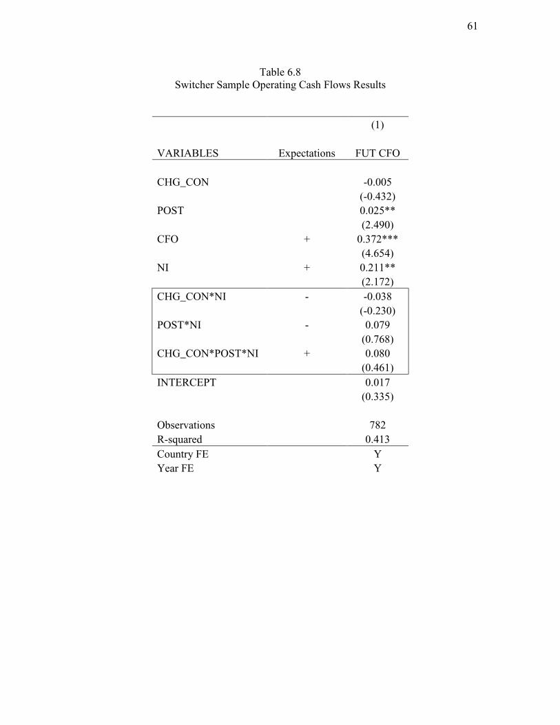
I supplement my cross-sectional findings by comparing the value relevance of

firms’ book value and earnings information for firms that switched measurement from

4

historical cost to fair value upon adoption of IAS 41, the “switcher” sample. The results

provide mixed evidence. Specifically, I find strong evidence that book value per share

became significantly more (less) value relevant for firms that held in-exchange (in-use)

biological assets and began measuring them at fair value upon adoption of the standard.

However, I find no other statistically significant results in the return tests or the

mechanical forecasting models of future operating cash flows and operating income. In

future work, I plan to hand-collect the interim fiscal year IAS 41 disclosures in order to

increase my sample, and consequently, the power of the switcher test.

Overall, my findings provide some empirical support for early accounting theory

that links value relevant asset measurement to the way in which the asset generates value

(e.g. Littleton 1935; May 1936). Further, my findings support the International

Accounting Standards Board’s (hereafter, IASB) recent proposed revisions to the

measurement section of its Conceptual Framework. Specifically, the IASB (2013a, ¶6.16)

proposes that the relevance and selection of a particular measurement basis depends on

how the asset contributes to the entity’s future cash flows, i.e. is used by the firm, and

this occurs either directly (i.e. in-exchange) or in combination with other assets (i.e. in-

use).

This paper makes several contributions to the literature. First, to my knowledge, it

is the first to test and provide empirical support for an asset measurement framework that

links asset measurement to asset use. This should be of interest to accounting standard

setters since the Financial Accounting Standards Board (hereafter, FASB) and the IASB

have voiced concern over their lack of a systematic framework to guide asset

5

measurement standards.1 As a result, asset measurement guidance continues to be a hotly

contested standard setting issue and inconsistencies exist across standards. 2 Thus, a

framework to guide standard setters’ asset measurement choices and to support high-

quality, consistent standard setting is greatly needed. I believe my findings provide

evidence supporting a systematic framework for asset measurement that could inform

standard setters’ decision-making processes on future asset measurement standards.

Second, my findings provide evidence that the asset measurement investors find

useful in assessing firm value is sometimes, but not always, fair value, and similarly for

historical cost. This is in contrast to the current academic debate over asset measurement,

which tends to side with either fair value or historical cost. Instead, my findings support

the IASB’s (2013a, ¶6.14) view on measurement bases which states, “… the IASB’s

preliminary view is the Conceptual Framework should not recommend measuring all

assets and liabilities on the same basis.” By understanding which asset measurement

investors find useful in determining firm value, the accounting community is better

positioned to understand cost-benefit tradeoffs and how to improve the effectiveness of

financial statement disclosures, a primary objective of the FASB’s disclosure framework

project (FASB 2012).

Finally, much of the prior literature examining fair value measurement

investigates whether fair value is sufficiently reliable to be value relevant to investors,

1 For example, the opening paragraph of the measurement section from the IASB’s (2013a, ¶6.1) discussion paper of its conceptual framework states: “The existing Conceptual Framework provides little guidance on measurement and when particular measurement should be used.” 2 The objective of the IASB and FASB’s joint project on an improved conceptual framework for financial reporting is “…for their standards to be clearly based on consistent principles. To be consistent, principles must be rooted in fundamental concepts rather than a collection of conventions” (as quoted in Milburn 2012; from IASB 2008, ¶4).

6

beyond measurement at historical cost.3 This relative reliability perspective differs from a

business valuation perspective, which links value relevant asset measurement to the

manner in which the asset realizes value, not to the relative reliability of the measure. In

contrast to the relative reliability research, I find that fair value information is more value

relevant for in-exchange biological assets than in-use biological assets, even after

controlling for cross-sectional differences in measurement reliability. That is, in my

study, value relevance is a function of asset use, not the reliability of the fair value

measure. 4 I seek to supplement and contribute to the extant literature by providing

evidence regarding the link between value relevant asset measurement and the manner in

which assets realize value.

3 See, for example, among others: Easton et al. 1993; Barth 1994a,b; Bernard et al. 1995; Barth et al. 1996; Barth and Clinch 1998; Aboody et al. 1999; Song et al. 2010. 4 The fair value of both in-exchange and in-use biological assets is often measured using a discounted cash flow approach, considered a “Level 3” estimation as defined by Statement of Financial Accounting Standard (SFAS) 157 (FASB 2006). Research suggests that investors perceive Level 3 estimates as less reliable than “Level 1” or “Level 2” estimates of fair value, which employ market prices (e.g. Kolev 2009; Song et al. 2010).

7

CHAPTER 2

LITERATURE REVIEW

2.1 Asset Measurement Frameworks

Prior research identifies standard setters’ lack of a systematic framework to guide

asset measurement standards as a weakness of the Conceptual Framework (see Agarwal

1987; Barth 2007; Barth 2014). The IASB explicitly acknowledges its lack of a

framework to guide asset measurement standards in the opening paragraph of the

measurement section of the IASB’s (2013a, ¶6.13) recent proposed revisions to its

Conceptual Framework, which states: “The existing Conceptual Framework provides

little guidance on measurement and when a particular measurement basis should be

used.” As a result, inconsistencies exist across asset measurement standards. For

example, under United States Generally Accepted Accounting Principles (hereafter, U.S.

GAAP) investment property is recognized at cost, while under IFRS, investment property

can be recognized at fair value (KPMG 2012). Similarly, under IFRS, PP&E can be

recognized at cost, but biological assets, which were formerly classified as PP&E and

measured at cost, are required to be recognized at fair value (KPMG 2012). As Cooper

(2007, 17) states, the lack of a measurement framework has resulted in, “… a large

number of different measurement bases applied in different standards, often with little

8

underlying logic.”5 Further, Barth (2014) argues that the Conceptual Framework’s lack of

measurement concepts is a major impediment to improving financial reporting.

A potential framework to guide asset measurement appears in early accounting

literature. Specifically, early accounting theorists link asset measurement to asset use (see

Littleton 1935; May 1936). In this literature, assets derive value either in-exchange or in-

use. Assets that derive value in-exchange do so on a standalone basis, independent of

other firm assets. The value of such assets to the firm is market driven with no

incremental value created by using the asset in combination with other assets. Examples

of in-exchange assets include financial securities or a tractor being held for sale. On the

other hand, assets that derive value in-use do so in combination with other firm assets

such that they create value incremental to the sum of the individual assets’ exchange

values. Examples of in-use assets include PP&E that is used for productive purposes.

Specifically, this literature argues that fair value applied to in-exchange assets and

historical cost applied to in-use assets has the potential to provide investors with

incrementally more value relevant information to forecast firm value (e.g. Littleton

1935).

Indeed, some modern-day accounting standards require different measurement

bases depending upon the firm’s use of the asset. For example, Statement of Financial

Accounting Standard (SFAS) 144 requires firms to recognize PP&E at the lower of its

carrying amount or fair value less costs to sell if the assets are being held for sale (FASB

2010). Otherwise, PP&E is recognized at cost on the balance sheet. Although some

5 In a similar sentiment, Barth (2014, 1) writes that as a result of the Conceptual Framework’s lack of a measurement framework, “…standard setting measurement decisions have been necessarily ad hoc and based more on historical precedent and the combined judgment of individual FASB and IASB members derived from experience, expertise, and intuition than on agreed upon measurement concepts.”

9

financial accounting standards link measurement to asset use, consistent with early

accounting theory, this approach has not been adopted at the Conceptual Framework

level. Further, there has been no empirical evidence on whether linking measurement to

asset use provides investors with more value relevant information. This paper provides an

empirical test of the theory.

In contrast to early accounting theory, advocates of fair value accounting propose

fair value as the value relevant measurement basis for both in-exchange and in-use assets,

as long as the fair value can be reliably estimated. Specifically, this research argues that if

fair value can be captured using quoted market prices, a Level 1 estimate from the fair

value measurement hierarchy defined by SFAS 157 (FASB 2006), it will provide

investors with value relevant information (e.g. Barth and Landsman 1995; Dietrich et al.

2000; Barth et al. 2001; Landsman 2007). Generally, fair value advocates argue that fair

value information is more relevant to investors than historical cost information for both

in-exchange and in-use assets (e.g. Barth et al. 2001; Landsman 2007).

2.2 Research on Fair Value Accounting

Consistent with both early accounting theory and fair value advocates, prior

empirical research has repeatedly established the value relevance of fair value

measurement for a specific class of in-exchange assets: financial securities.6 Moreover,

these findings extend to investors’ use of fair value measurement information for

financial securities under all three levels of the fair value measurement hierarchy defined

by SFAS 157: quoted prices for identical assets (Level 1), quoted prices of similar assets

6 These studies consistently find that investors perceive fair value estimates for financial securities as more value relevant than historical cost amounts: Barth 1994a, b; Ahmed and Takeda 1995; Bernard et al. 1995; Petroni and Whalen 1995; Barth et al. 1996; Eccher et al. 1996; Nelson 1996.

10

(Level 2), and fair value measured using valuation techniques (Level 3) (Kolev 2009;

Song et al. 2010). Consistent with these findings, recent research finds no difference in

the value relevance of Level 1 versus Level 3 inputs for financial securities (Lawrence et

al. 2014), and that Level 3 inputs best capture the underlying cash flows generated from

financial securities when markets are inactive (Altamuro and Zhang 2013). Accordingly,

the value relevance of fair value information is not simply a function of measurement

reliability.

The empirical research on the relevance of fair value for financial securities

provides the strongest evidence in favor of fair value as the value relevant measurement

basis. Financial securities, however, derive value in-exchange, not in-use. Therefore, the

fair value research on financial securities does not distinguish between the two asset

measurement frameworks, early accounting theory versus fair value advocates: there is

little variation in the manner in which financial securities are expected to realize value for

the firm. Moreover, whether fair value provides investors with value relevant information

for in-exchange assets that are not financial securities is an empirical question that I test

in this paper.

Empirical research regarding equity investors’ use of fair value measurement for

nonfinancial assets provides mixed findings. First, the studies do not clarify whether the

nonfinancial assets derive value in-use or in-exchange. Second, the research examining

the value relevance of fair value for nonfinancial assets is burdened by the lack of

mandated measurement variation across in-use asset classes. Accordingly, early research

examining investors’ use of fair value information for in-use assets examines disclosed

current cost estimates for firms’ PP&E required under SFAS 33. Collectively, this

11

research fails to find that current cost disclosures are value relevant (e.g. Beaver and

Landsman 1983; Beaver and Ryan 1985; Bernard and Ruland 1987; Hopwood and

Schaefer 1989; Lobo and Song 1989). The lack of relevance, however, could be

attributed to investors’ perceptions of disclosed values as less reliable or relevant than

recognized amounts (see Ahmed et al. 2006).

Later empirical research examining investors’ use of fair value measurement for

nonfinancial assets employs settings in which United Kingdom (hereafter, U.K.) and

Australian firms made discretionary revaluations to their tangible long-lived assets.

Generally, this research provides evidence that investors find the asset revaluations value

relevant in stock price and return estimations (e.g. Easton et al. 1993; Barth and Clinch

1998) and in mechanical forecasting models of future operating cash flows and operating

income (Aboody et al. 1999). However, a problem drawing inferences from the

discretionary asset revaluation research is that managers decide to revalue ex-post and

therefore may revalue for a host of reasons that are unrelated to providing investors with

value relevant information, i.e. when they need to manage reported performance

(Christensen and Nikolaev 2013). Again, the studies do not clarify whether the

nonfinancial assets in question derive value in-use or in-exchange.

More recent empirical research on fair value measurement of nonfinancial assets

examines firms’ measurement choice for nonfinancial assets upon adoption of IFRS.

Both Cairns et al. (2011) and Christensen and Nikolaev (2013) find that few U.K.,

Australian, and German firms choose to measure their nonfinancial assets at fair value

upon adoption of IFRS. Instead, Christensen and Nikolaev (2013) find that firms almost

exclusively choose historical cost measurement for intangibles and PP&E asset classes

12

(i.e. in-use assets).

Some research attributes the mixed evidence on the relevance of fair value

measurement for nonfinancial assets to the lack of reliability of the fair value estimates

(e.g. Barth et al. 2001). Instead, I argue that prior research has not carefully considered

the role asset use might play in determining which asset measurement basis is value

relevant. Thus, the mixed results could be linked to the confounding factor of asset use as

opposed to variation in the reliability of the estimates. I empirically test whether fair

value or historical cost measurement for in-use assets provides investors with more value

relevant information on a sample of firms that adopt IAS 41.

2.3 Research on Historical Cost Accounting

Unlike the research on fair value accounting for nonfinancial assets, there is little

empirical research on the value relevance of historical cost for in-use assets. Most of the

literature arguing that historical cost may provide investors with value relevant

information for in-use assets relies on business valuation theory, including Littleton

(1935) and May (1936). Specifically, this literature focuses on the information investors

require to forecast the cash flows in-use assets generate. For example, Deans (2007, 31)

argues, “…it is harder to see how knowing the fair values (exit values) of [in-use] assets

that generate cash flows helps in forecasting those cash flows.” Cooper (2007, 17) argues

that while historical cost may not be relevant when making an economic decision with

respect to a specific asset, for example deciding whether to sell an asset, not all decisions

are made on an asset-by-asset basis. Instead, Cooper (2007) argues that for in-use assets,

assets that are used in combination with other assets in a business venture and where

13

immediate sale is not intended, historical cost best captures the overall profitability of the

business venture.

In addition, Nissim and Penman (2008) maintain that historical cost accounting is

designed for business models where the firm transforms inputs to add value, i.e. in-use

assets. Similarly, a measurement framework developed by the Institute of Chartered

Accountants in England and Wales (2010) advocates for historical cost accounting as the

most relevant measurement basis when the firm’s business model is to transform inputs

so as to create new assets or services as outputs, i.e. in-use assets. Additionally, Botosan

and Huffman (2014) argue that historical cost provides investors with relevant

information for in-use assets because historical cost information is useful to investors in

forecasting the future cash flows from in-use assets. Finally, the IASB (2013a, ¶6.16b)

states that for assets deriving value in-use, investors may find historical cost more

relevant than fair value because historical cost preserves the margins generated by past

transaction that investors find useful in estimating future margins to forecast the cash

flows in-use assets generate. The IASB (2013a, ¶6.16b) states, “Changes in the market

price of [in-use assets]… may not be particularly relevant for this purpose.”

Whether asset measurement linked to asset use provides investors with value

relevant information is an empirical question I test in this paper. In particular, whether

fair value measurement provides investors with value relevant information for in-

exchange assets that are not financial securities, and whether fair value or historical cost

measurement provides investors with value relevant information for in-use assets remain

open empirical questions in the literature. I examine early accounting theory’s proposal

14

that measurement linked to asset use provides investors with value relevant information

on a sample of firms that adopt IAS 41.

15

CHAPTER 3

MOTIVATION AND HYPOTHESES

3.1 IAS 41 Background

The International Accounting Standards Committee, the IASB’s predecessor,

issued IAS 41 in 2001 in order to develop more uniform accounting practices for

agricultural activities (IASB 2006). The standard became effective for annual reporting

periods beginning on or after January 1, 2003, or alternatively, upon adoption of IFRS.

IAS 41 prescribes accounting treatment for biological assets, which are living plants and

animals. 7 Biological assets are held by firms involved in agricultural activity.

Agricultural activities that produce or employ biological assets include raising livestock,

forestry, cropping, cultivating orchards and plantations, floriculture, and aquaculture

(IASB 2009, ¶6).

Prior to the passage of IAS 41, agricultural activity was excluded from the scope

of international accounting standards (IASB 2012, ¶8). Accounting guidelines for

agricultural activities were developed by national standard setters on a piecemeal basis to

resolve specific issues (IASB 2012, ¶8b). Pre-IAS 41, most firms accounted for their

biological assets at historical cost and classified the assets as PP&E on the balance sheet.

7 Specifically, IAS 41 prescribes accounting treatment for agricultural activity, or “management by the entity of the biological transformation of living animals and plants (biological assets) for sale, into agricultural produce, or into additional biological assets” (IASB 2009, ¶IN1).

16

Consequently, the assets were subject to impairment analysis. Upon adoption of the

standard, however, firms line item the value of their biological assets on the balance

sheet, separate from PP&E.

The passage of IAS 41 offers a unique setting to test whether asset measurement

linked to asset use provides investors with value relevant information, for several reasons.

First, variation exists in the manner in which firms employ their biological assets to

realize value. Specifically, IAS 41 encourages firms to distinguish between “consumable”

and “bearer” biological assets in order to provide information that may help investors to

assess the timing of future cash flows (IASB 2009, ¶43). This distinction maps closely

into the way in which the biological assets are expected to realize value for the firm.

Consumable biological assets are agricultural products, like crops or timber, or sold as

biological assets, like commodities (IASB 2009, ¶44). Consumable biological assets

realize value on a standalone basis and their value to the firm is linked to what the asset

might be exchanged for in the marketplace. Thus, these assets are closer in nature to in-

exchange assets. Bearer biological assets, on the other hand, are self-regenerating assets,

like orchards or oil palm plantations (IASB 2009, ¶44), which are employed in

combination with other assets in the on-going operations of the firm. Thus, bearer

biological assets realize value in combination with other assets and are therefore closer in

nature to in-use assets. I employ IAS 41’s definition of consumable and bearer biological

assets to proxy for the assets’ value realization, either in-exchange or in-use, respectively.

Second, IAS 41 provides a setting with mandated measurement variation. Prior to

adoption of IAS 41, firms measured their biological assets at historical cost and classified

them as PP&E. IAS 41 requires firms to measure their biological assets at fair value,

17

although the standard allows firms to measure their biological assets at historical cost if

the firm is able to demonstrate that the fair value of its biological assets cannot be reliably

estimated, i.e. there is a lack of reliable parameters such as known prices, growth rates, or

physical volumes of the asset (IASB 2009, ¶30). I utilize this measurement variation in

my research design. Specifically, 41% (789 observations) of the firm-year observations in

my sample contain biological assets measured at cost, while 41% of the firm-year

observations contain biological assets measured at fair value (see Figure 3.1). Of the cost

sample, 237 observations are post-IAS 41 firm-year observations where firms applied the

historical cost stipulation. The measurement variation in the sample of firms that apply

the historical cost stipulation postadoption of IAS 41 appears to be driven at the country

level. Specifically, it appears that certain countries are enforcing IAS 41 as mandated,

like the United Kingdom, while other countries are allowing firms to apply the historical

cost stipulation within the standard. I include country fixed-effects in my estimations to

control for this variation, and I also explore the effects of audit enforcement of

accounting standards in robustness tests.

Finally, IAS 41 is a “true” fair value standard. That is, the firms that measure their

biological assets at fair value must recognize the value on their balance sheets and any

change in the value of the assets over the reporting period, unrealized gains or losses, in

income. Therefore, IAS 41 provides variation in asset measurement while helping to

mitigate issues related to investors’ perceptions of recognized versus disclosed amounts

when firms fair value in-use assets in disclosures (e.g. Beaver and Landsman 1983;

Ahmed et al. 2006), or when provided a choice (Cairns et al. 2011; Christensen and

Nikolaev 2013).

18

Under IAS 41, a firm producing palm oil from oil palm trees measures its oil palm

plantations, an in-use asset, at fair value on the balance sheet, excluding any fair value

attributable to the land upon which the oil palms are physically attached or intangible

assets related to the oil palm production (IASB 2009, ¶2). Thus, firms are required to

measure and report only the oil palm trees component of the in-use assets, not the land or

intangible assets related to the production of the palm oil, at fair value. Likewise, a firm

that harvests logs from timber plantations, an in-exchange asset, also measures the timber

plantations at fair value every reporting period on the balance sheet, less any costs to sell.

Changes in the fair value of the oil palm plantations or timber (i.e. unrealized holding

gains and losses) are recognized in periodic income (IASB 2009).

Unlike IFRS, the term “biological assets” does not exist in U.S. GAAP or in its

accounting for agricultural producers (KPMG 2012). Instead, the terms “growing crops”

and “animals being developed for sale” are used to describe what would be called

biological assets under IFRS (KPMG 2012). Under U.S. GAAP, growing crops and

animals being developed for sale can be stated at the lower of cost or market, or at sales

price less costs to sell if the following criteria are met: the product has a determinable

market price, insignificant costs of disposal, and is available for immediate delivery

(KPMG 2012). It is interesting to note that assets with these characteristics are closer in

nature to in-exchange assets and when a sufficiently reliable measure of fair value exists,

U.S. GAAP allows such assets to be reported at fair value determined based on exit value

less cost to sell.

Recently, the Asian-Oceanian Standard Setters Group (AOSSG) proposed

different accounting treatments for bearer and consumable biological assets because of

19

the differences in the way the asset-types are used by the firm (IASB 2012). Specifically,

the AOSSG Issues Paper (IASB 2012) argues that bearer biological assets are held for

income generation (derive value in-use) and therefore should be treated as PP&E, which

allows for measurement at cost, while consumable biological assets are held for sale

(derive value in-exchange), and as such should continue to be measured at fair value.

Moreover, the paper surveys a group of analysts specializing in plantation valuations, a

type of bearer biological asset. The paper reports that the analysts did not find the

reporting of the fair value of bearer biological assets as useful because the fair value,

“…distorts the financial statements’ ability to reflect a ‘true & fair’ view of an agriculture

company’s earnings” (IASB 2012, ¶32a). Further, the analysts said that, “… they always

remove the biological gains or losses [from bearer biological assets] when looking at

earnings and that end-users also do not look at fair value” (IASB 2012, ¶33).

In response to the AOSSG Issues Paper (IASB 2012), the IASB recently issued an

Exposure Draft (IASB 2013b) proposing to amend IAS 41 with respect to a specific class

of bearer biological assets: bearer plants.8 Consistent with the framework I test in this

paper, the Exposure Draft (IASB 2013b, ¶BC2) asserts that bearer plants are similar to

PP&E, and as such, should be accounted for under IAS 16, the standard that prescribes

measurement for PP&E, and allows for measurement at historical cost. The Exposure

Draft (IASB 2013b, ¶BC5) argues that investors, analysts, and other users of financial

statements did not find the fair values of bearer plants useful and would adjust reported

statements to eliminate the effects of the fair value accounting. Further, the Exposure

Draft (IASB 2013b) does not propose disclosing fair value amounts for bearer plants.

Nevertheless, under IAS 41, firms measure both in-exchange and in-use 8 The proposed amendment to IAS 41 does not include bearer livestock, like dairy cattle, only plants.

20

biological assets at fair value, and at historical cost. This allows for cross-sectional tests

of comparison of firm-year observations where measurement is consistent with asset use

(the consistent measurement sample), i.e. where in-exchange biological assets are

measured at fair value and in-use biological assets are measured at historical cost, and

firm-year observations where measurement is inconsistent with asset use (the inconsistent

measurement sample), i.e. where in-exchange biological assets are measured at historical

cost and in-use biological assets are measured at fair value.

3.2 Main Hypothesis

I examine whether asset measurement linked to asset use provides investors with

relatively more value relevant information to assess firm value than asset measurement

that is not linked to asset use. In their joint Conceptual Framework for financial reporting,

the FASB and the IASB characterize financial information as decision-useful if it is

relevant and faithfully represents what it purports to represent (IASB 2010, ¶QC4).

Relevant information, as characterized by the Conceptual Framework, is financial

information that is capable of making a difference in the decisions made by users, i.e. it

has predictive or confirmatory value, or both (IASB 2010, ¶QC6-¶QC7). I adopt this

characterization of value relevant financial reporting information in my empirical tests,

and I focus on the value relevance of financial reporting information to investors.9

Consequently, my main hypothesis examines the relative value relevance of

9 I recognize that the information needs of some users of financial reporting information are driven by economic decisions that are not informed by an assessment of firm value. I focus on the information needs of users interested in assessing firm value because a rigorous consideration of the information needs of all users is impractical. Moreover, I believe the users I focus on comprise an important set. This is supported by Dichev et al. (2012), who find that 94.7% of the public company CFOs they surveyed identify valuation as the primary reason earnings are important to users.

21

firm’s financial statement information when biological assets are measured consistent

with their use, relative to when they are not:

H1: Asset measurement consistent with biological assets’ use provides investors with more value relevant information than measurement that is inconsistent with the biological assets’ use.

22

Measurement

FV HC TOTAL

Value Realization

IN-USE 343 607 950

25% 45% 70%

IN-EXCH 216 182 398

16% 14% 30%

TOTAL 559 789 1,348

41% 59% 100%

Figure 3.1 Value Realization and Measurement Sample Composition for the

Cross-Sectional Sample

23

CHAPTER 4

RESEARCH DESIGN

I adopt a multipronged approach to test my hypothesis. I first employ cross-

sectional tests, where I examine value relevance regressions of stock price and returns,

and mechanical forecasting models of operating cash flows and operating income for the

sample of firms that measure their biological assets consistent with their use compared to

the sample of firms that measure their biological assets inconsistent with the assets’ use. I

estimate the cross-sectional tests on firm-year observations pre-IAS 41, where firms

measured their biological assets at historical cost and classified them as PP&E, and on

firm-year observations post-IAS 41 adoption.

I include pre-IAS 41 observations in my cross-sectional tests for two reasons.

First, pre-IAS 41, measurement at historical cost was not a choice: all firms measured

their biological assets at historical cost, as part of PP&E. This avoids the potential

selection bias of including only post-IAS 41 historical cost observations, where firms

apply the historical cost stipulation to measure their biological assets at historical cost

instead of fair value. Second, including the pre-IAS 41 data allows for a larger sample of

historical cost observations: 789 observations (see Figure 3.1) versus 237 observations if

I only include the post-IAS 41 sample. This increases the power of my tests and

24

therefore, the potential inference to be made regarding value relevant asset measurement

and asset use.

Next, I examine the value relevance of book value and earnings information for

the “switcher” sample, the sample of firms that pre-IAS 41 measured their biological

assets at historical cost and then switched measurement to fair value upon adoption of the

standard. Figure 4.1 illustrates the approach. As described earlier, prior to IAS 41, firms

measured their biological assets at historical cost and classified them as PP&E.

Therefore, the adoption of IAS 41 provides a setting where firms that held in-exchange

biological assets measured them inconsistent with their use pre-adoption, but then

switched measurement to fair value consistent with the biological asset’s use. Similarly,

in the pre-adoption period, some firms measured their in-use assets consistent with their

use (at historical cost) and then postadoption, began measurement of their in-use assets

inconsistent with their use (measured at fair value). I again estimate value relevance

regressions of stock price and returns, and mechanical forecasting models of operating

cash flows and operating income for the switcher sample. I limit my sample to firm-year

observations with at least one year of pre-IAS 41 data.

In both my cross-sectional and switcher tests, I include no more than five years of

pre-IAS 41 data for the following reason. I assume that the type of biological assets the

firm held upon adoption of IAS 41, either in-use or in-exchange, are the type of

biological assets that the firm held in the prior five years since these data are

unobservable in the pre-IAS 41 period. If one assumes that a firm’s business model is

stable over more than five years, this is a conservative assumption in that it excludes

observations, which might otherwise be valid. Nevertheless, this assumption allows me to

25

better ensure that my inferences with respect to the pre-IAS 41 data are driven by the

value relevance of the biological assets, not other unrelated asset or business choices the

firm might have made in a preperiod of greater length than five years.10 Further, several

of the firms in my sample have close to 20 years of pre-IAS 41 data. By restricting the

pre-IAS 41 data to five years, I can better ensure that one firm’s data or a limited sample

of firms are not driving my results.

4.1 Consistent and Inconsistent Measurement Samples

I sort firm-year observations into the consistent and inconsistent measurement

samples in the following manner. I employ IAS 41’s definition of consumable and bearer

biological assets to represent in-exchange and in-use biological assets, respectively. To

be classified as consistent, I group firm-year observations where in-exchange biological

assets are measured at fair value (216 firm-year observations) or in-use biological assets

are measured at historical cost (607 firm-year observations) (see Figure 3.1). To be

classified as inconsistent, I group firm-year observations where in-use biological assets

are measured at fair value (343 firm-year observations) or in-exchange biological assets

are measured at historical cost (182 firm-year observations) (see Figure 3.1). Recall that

for the pre-IAS 41 historical cost data, I assume that the type of biological assets the firm

held in the year it adopted IAS 41, either in-use or in-exchange, is the type of biological

assets the firm held in the pre-adoption period.

My sample is limited to firm-year observations drawn from firms for which all of

their biological assets are measured on a consistent or inconsistent basis. Mixed

measurement firms are those which measure some biological assets on a consistent basis 10 My results are unchanged if I include fewer than five years of pre-IAS 41 data.

26

and some on an inconsistent basis. I exclude firm-year observations from such mixed

measurement firms (270 firm-year observations). I do so to ensure clear predictions

regarding my measurement samples. This provides a sample of 823 firm-year

observations for the consistent measurement sample and 525 firm-year observations for

the inconsistent measurement sample.

4.2 Interpretation of the Results

For the cross-sectional tests, I estimate all models on the pooled sample and then

separately by measurement basis. I evaluate results in the following manner. If value

relevant asset measurement is linked to asset use, then I expect the variables for the

consistent sample, in the stock price and return models and the mechanical forecasting

models of operating cash flows and operating income, to be incrementally more

significant than the variables for the inconsistent sample. Specifically, the evidence

would suggest that firm inputs are relatively more predictive of firm performance when

measurement is consistent with asset use (the consistent sample), relative to when it is not

(the inconsistent sample).

In the switcher sample design, I expect that postadoption of IAS 41, the value

relevance of firms’ book value and earnings information will significantly improve for

the sample of firms that held in-exchange biological assets and began measuring them at

fair value upon adoption of the standard. On the other hand, I expect that postadoption of

IAS 41, the value relevance of firms’ book value and earnings information will

significantly decline for the sample of firms that held in-use biological assets and upon

adoption of IAS 41 measured the assets at fair value. This would provide evidence in

27

support of my hypothesis, that measurement linked to asset use provides investors with

relatively more value relevant information than asset measurement that is not linked to

asset use.

4.3 Price and Return Tests

I follow prior value relevance research and examine value relevance regressions

of price and returns. In a vein similar to Easton et al. (1993), Barth and Clinch (1998),

and Aboody et al. (1999), I estimate the following cross-sectional model on the pooled

sample and then by measurement basis:

��,� � �� ��� �������,� ������,� ���� � �����,� �� �4.1�

In model (4.1), ��,� is the share price for firm i one month following the annual

report filing or, alternatively, four months following the end of the firm’s fiscal year-

end; �� is a dummy variable that takes the value of one for firm-year observations

classified in the consistent measurement sample; �����,� is the firm’s book value per

share at the end of the fiscal year; and ����,� is earnings per share at fiscal year-end

excluding any unrealized gains or losses (URGL) related to the fair value of the

biological assets recognized in income. I include the URGL related to the fair value of the

biological assets in the BVPS term because this is the variable I interact with CON in

testing my hypothesis. I include the interaction term to examine whether firms’ book

value is incrementally more value relevant when biological assets are measured

consistent with their use, i.e. the consistent measurement sample, relative to when they

28

are not, i.e. the inconsistent sample.

I then estimate a variation of model (4.1) for the switcher sample:

��,� � �� ����_�� ������ �������,� ������,�

� ���_�� � �����,� �!���� � �����,�

�"���_�� � ���� � �����,� �� �4.2�

In model (4.2), POST is an indicator variable that takes a value of one if the firm-

year observation falls in the post-IAS 41 period and CHG_CON is an indicator variable

that takes a value of one if the firm holds in-exchange biological assets. All other

variables are defined above. In model (4.2), the variables of interest are: � which

captures the value relevance of BVPS pre-IAS 41 for firms that held in-exchange

biological assets and measured them at cost; �! which captures the value relevance of

BVPS post-IAS 41 for firms that held in-use biological assets and measured them at fair

value; and finally, �" which captures the value relevance of BVPS post-IAS 41 for firms

that held in-exchange biological assets and measured them at fair value. If my hypothesis

is supported, I expect �" to be significantly positive, and I expect � and �! to be

significantly negative. These findings would suggest that firms’ BVPS significantly

increased in value relevance once firms’ that held in-exchange biological assets began

measuring them at fair value (�"), compared to when firms measured their in-exchange

biological assets at historical cost pre-IAS 41 (� ), and firms that held in-use biological

assets and began measuring them at fair value postadoption of IAS 41 experienced a

decline in the value relevance of their BVPS (�!).

29

I also include the changes estimation of model (4.1), following Easton et al.

(1993), Barth and Clinch (1998), and Aboody et al. (1999). Specifically, I estimate the

following cross-sectional model on the pooled sample and then by measurement basis:

$%&�,� � �� ��� �� '�,� ��( '�,� ���� � '�,� �� �4.3�

In model (4.3), $%&�,� is the firm i's cumulative 12-month raw return ending the

month following the annual report filing or, alternatively, four months following the end

of the firm’s fiscal year-end; '�,� is the firm’s net income for the fiscal year; and ( '�,�

is the change in net income over the fiscal year. I include the interaction term to examine

whether net income is incrementally more value relevant for firm returns when

measurement is consistent with asset use. All variables are deflated by beginning period

market value of equity.

Finally, I estimate a variation of model (4.3) for the switcher sample:

$%&�,� � �� ����_�� ������ �� '�,� ��( '�,� � ���_�� � '�,�

�!���� � '�,� �"���_�� � ���� � '�,� �� �4.4�

All variables are defined above. In model (4.4), the variables of interest are: �

which captures the value relevance of firms’ NI pre-IAS 41 for firms that held in-

exchange biological assets and measured them at cost; �! which captures the value

relevance of firms’ NI post-IAS 41 for firms that held in-use biological assets and

30

measured them at fair value; and finally �" which captures the value relevance of firms’

NI post-IAS 41 for firms that held in-exchange biological assets and measured them at

fair value. If my hypothesis is supported, I expect �" to be significantly positive, and I

expect � and �! to be significantly negative. These findings would suggest that firms’

NI significantly increased in value relevance once firms that held in-exchange biological

assets began measuring them at fair value (�"), compared to when firms measured their

in-exchange biological assets at historical cost pre-IAS 41 (� ), and firms that held in-use

biological assets and began measuring them at fair value postadoption of IAS 41

experienced a decline in the value relevance of their NI (�!).

I estimate standard errors clustered by firm for models (4.1)-(4.4) and I winsorize

the price and return samples at the second and 98th percentiles to minimize the influence

of outliers. In addition, I include country and year fixed effects in all estimations in order

to control for unobservable, confounding variables that differ across firms, but are

constant over time and across country.

4.4 Mechanical Forecast Models

I examine whether asset measurement linked to asset use influences the ability of

a mechanical forecasting model of firms’ future operating cash flows and operating

income. I follow prior international accounting research to estimate forecasts of both

operating cash flows and income (e.g. Barth et al. 2012). The operating cash flows model

for the cross-sectional test appears below, which I estimate on the pooled sample and

then by measurement basis:

31

�*�,�+ � , ��� ���*�,� �� '�,� ���� � '�,� ��,� (4.5)

where net operating cash flows for firm i , �*�+, one period ahead of fiscal year t are a

function of: operating cash flows for fiscal year t, �*�,�; and '�,� net income for fiscal

year t. In addition to future operating cash flows, I estimate model (4.5), including the

sum of future operating cash flows one, two, and three periods ahead of fiscal year t, as

the dependent variable. I include the interaction term to examine whether net income is

incrementally more predictive of future operating cash flows when measurement is

consistent with asset use. All variables are deflated by average total assets.

I estimate a variation of model (4.5) for the switcher sample:

�*�,�+ � �� ����_�� ������ ���*�,� �� '�,� � ���_�� � '�,�

�!���� � '�,� �"���_�� � ���� � '�,� �� �4.6�

All variables are defined above. In addition to future operating cash flows, I

estimate model (4.6), including the sum of future operating cash flows one, two, and

three periods ahead of fiscal year t, as the dependent variable. In model (4.6), the

variables of interest are: � which captures the value relevance of firms’ NI pre-IAS 41

for firms that held in-exchange biological assets and measured them at cost; �! which

captures the value relevance of firms’ NI post-IAS 41 for firms that held in-use biological

assets and measured them at fair value; and finally �" which captures the value relevance

of firms’ NI post-IAS 41 for firms that held in-exchange biological assets and measured

them at fair value. If my hypothesis is supported, I expect �" to be significantly positive,

32

and I expect � and �! to be significantly negative. These findings would suggest that

firms’ NI significantly increased in value relevance once firms’ that held in-exchange

biological assets began measuring them at fair value (�" ), compared to when firms

measured their in-exchange biological assets at historical cost pre-IAS 41 (� ), and firms

that held in-use biological assets and began measuring them at fair value postadoption of

IAS 41 experienced a decline in the value relevance of their NI (�!).

The operating income model I estimate for the cross-sectional test appears below,

which I estimate on the pooled sample and then by measurement basis:

��_' ��,�+ � , ��� ����_' ��,� ����_' ��,�. ���� �

��_' ��,� ��,� (4.7)

where operating income for firm i, �/_' ��,�+, one period ahead of fiscal year t is a

function of: the current period’s operating income, �/_' ��,� ; and lagged operating

income, �/_' ��,�.. I calculate operating income using the S&P Capital IQ variable

“earnings from continuing operations,” which includes unrealized gains and losses

related to biological assets. Again, I include the interaction term to examine whether

operating income is incrementally more predictive of future operating income when

measurement is consistent with asset use.

I estimate a variation of model (4.7) for the switcher sample:

33

��012�,�+� �� ����_�� ������ ����012�,�

����012�,�.

� ���_�� � ��012�,� �!���� � ��012�,�

�"���_�� � ����

� ��012�,� �� �4.8�

All variables are defined above. In model (4.8), the variables of interest are: �

which captures the value relevance of firms’ OP_INC pre-IAS 41 for firms that held in-

exchange biological assets and measured them at cost; �! which captures the value

relevance of firms’ OP_INC post-IAS 41 for firms that held in-use biological assets and

measured them at fair value; and finally �" which captures the value relevance of firms’

OP_INC post-IAS 41 for firms that held in-exchange biological assets and measured

them at fair value. If my hypothesis is supported, I expect �" to be significantly positive,

and I expect � and �! to be significantly negative. These findings would suggest that

firms’ OP_INC significantly increased in value relevance once firms that held in-

exchange biological assets began measuring them at fair value (�"), compared to when

firms measured their in-exchange biological assets at historical cost pre-IAS 41 (� ), and

firms that held in-use biological assets and began measuring them at fair value

postadoption of IAS 41 experienced a decline in the value relevance of their OP_INC

(�!).

All variables in models (4.5)-(4.8) are deflated by average total assets and are

winsorized at the second and 98th percentiles to minimize the influence of outliers. I

estimate all standard errors clustered by firm. In addition, I include country and year

fixed effects in all estimations in order to control for unobservable, confounding variables

that differ across firms, but are constant over time and across country.

34

IAS 41 PRE-IAS 41 POST-IAS 41

CHG_CON=1 In-Exchange Bio Assets

Historical Cost

Fair Value

CHG_CON=0 In-Use Bio Assets

Historical Cost

Fair Value

Figure 4.1 Switcher Sample Research Design

35

CHAPTER 5

SAMPLE SELECTION AND DESCRIPTIVE STATISTICS

5.1 Sample Identification and Data Sources

I identify firms that hold biological assets by conducting a word search in the

Morningstar Document Research Global Report’s subscription and in the S&P Capital

IQ databases. I search on the phrase “biological assets.” I supplement this search with a

report issued by the Institute of Charted Accountants of Scotland that lists Australian,

U.K., and French firms that hold biological assets (see Elad and Herbohn 2011, Appendix

1). I restrict the Morningstar and the S&P Capital IQ searches to annual report filings. I

then eliminate firms with biological assets that comprise less than 5% of the firm’s total

assets (433 firm-year observations). I eliminate firm-year observations where book equity

is negative (11 firm-year observations). I further eliminate firms that have less than $1

million U.S. Dollars (USD) in total assets, or fewer than five years of financial statement

data available on the S&P Capital IQ database to eliminate outliers from my estimations

that may have undue influence on the results (55 firm-year observations).

I hand-collect the IAS 41 data. Specifically, for each fiscal year in my sample, I

hand-collect the following amounts: the balance sheet value of the biological assets; any

URGL related to the change in the fair value of the biological assets recognized on the

36

income statement or in the footnote; the classification of the biological assets as

consumable or bearer; and whether the firm measures the biological assets at fair value or

historical cost. I collect all financial statement data from S&P Capital IQ and I collect all

price and return data from Datastream.

For firms that are cross-listed on different exchanges, I calculate the price and

return variables using aggregated market data.11 Specifically, I sum the market value and

the shares outstanding across all cross-listed market exchanges. I then calculate an

aggregate firm price by dividing the aggregated market cap by the aggregated shares

amount. I calculate an aggregate firm return by value-weighting the monthly returns from

all the cross-listed market exchanges by market cap.

I pull all financial statement, price, and return data converted to USD from the

respective databases. The hand-collected data, on the other hand, are reported in the filing

currency. I convert the hand-collected amounts to USD using the ratio of S&P Capital

IQ’s total assets reported in the firm’s filing currency to S&P Capital IQ’s total assets

reported for the firm in USD to calculate a historical conversion rate. This way I convert

the hand-collected amounts using the same historical conversion rate S&P Capital IQ

used for the other firm financial statement data. I convert all data to USD for descriptive

ease.

5.2 Descriptive Statistics

Figure 5.1 provides the sample composition for the switcher sample by pre- and

postadoption periods, and value realization, either in-use or in-exchange. Recall that

firms are included in the switcher sample if they have at least one year and no more than 11 Fifty-five percent of firms in the sample are cross-listed on a variety of other exchanges.

37

five years of preperiod data. This provides a sample of 154 firms. The majority of the

sample holds in-use assets (66%). Further, preperiod data account for 42% of the sample

while postadoption data account for 58% of the sample.

Table 5.1 provides descriptive statistics for the composition of the cross-sectional

sample by country. The sample is comprised of 182 firms from 33 different countries (see

Table 5.1). Approximately 42% of the firms in the sample are located in Australia,

Malaysia, or Singapore. Table 5.2 provides descriptive statistics for the composition of

the cross-sectional sample by fiscal year and measurement basis. The cross-sectional

sample spans 1996-2011 (see Table 5.2). The historical cost observations comprise the

early years of the sample while the fair value sample is concentrated in the latter half of

the sample period, coinciding with the increased country-level adoption of IFRS. The fair

value firm-year observations from 1999-2001 are Australian firms that reported the fair

value of their regenerating and self-generating assets under the Australian standard

AASB 1037 that predated IAS 41. I include these observations in the sample because

they provide variation in value realization and asset measurement.12

Table 5.3 provides descriptive statistics for the cross-sectional sample that

measures their biological assets at fair value. The descriptive statistics are presented by

consistent and inconsistent measurement sample. All data are reported in USD and

winsorized at the second and 98th percentiles to reduce the influence of outliers on results.

Results from t-statistic tests of differences in means and medians between the consistent

and inconsistent samples are reported in the consistent sample tables.

Table 5.3 shows that consistent sample of firms that measure their biological

assets at fair value is significantly less profitable, on average and at the median, in terms 12 My findings are robust to the exclusion of the firm-year observations that pre-date IAS 41.

38

of operating cash flows ($0.03 versus $0.05), net income ($0.02 versus $0.05), operating

income ($0.02 versus $0.05), and future operating income ($0.03 versus $0.06). This

finding is possibly related to the difference in firms’ business models. Specifically, firms

that hold in-exchange assets (the consistent sample) are less profitable than firms that

hold in-use assets (the inconsistent sample) because firms with in-use assets take on more

risk and therefore require a higher return: in-use assets (bearer biological assets) take

longer to produce future revenue than in-exchange assets (consumable biological assets).

There is no significant difference at the mean between the consistent and inconsistent

samples for the price and return variables. Further, both the consistent and inconsistent

samples hold on average 25% of biological assets comprising total assets. In addition,

both samples have average price per share of approximately $5.00.

Table 5.4 provides descriptive statistics for the cross-sectional sample that

measures their biological assets at historical cost. The descriptive statistics are presented

by consistent and inconsistent measurement sample. All data are reported in USD and

winsorized at the second and 98th percentiles to reduce the influence of outliers on results.

Results from t-statistic tests of differences in means and medians between the consistent

and inconsistent samples are reported in the consistent sample tables.

Table 5.4 shows that consistent sample of firms that measure their in-use

biological assets at historical cost is significantly larger in terms of observations for the

price and return estimations: 440 observations for the consistent sample versus 85

observations for the inconsistent sample. The sample is comprised of few firms that

measure their in-exchange biological assets at historical cost. Nevertheless, the consistent

sample is more profitable, on average, than the inconsistent sample in terms of EPS

39

($0.08 versus $0.01), and returns (0.26 versus 0.17). This finding is again consistent with

differences in firms’ business models. Specifically, firms that hold in-use assets (the

consistent sample) are more profitable and have a higher return than firms that hold in-

exchange assets (the inconsistent because firms with in-use assets take on more risk and

require a higher return: in-use assets (bearer biological assets) take longer to produce

future revenue than in-exchange assets (consumable biological assets). There is no

significant difference between the two samples with respect to mechanical forecasting

model variables.

Table 5.5 provides descriptive statistics for the switcher sample. The descriptive

statistics are presented by consistent and inconsistent measurement sample. All data are

reported in USD and winsorized at the second and 98th percentiles to reduce the influence

of outliers on results. Results from t-statistic tests of differences in means and medians

between the consistent and inconsistent samples are reported in the consistent sample

tables.

Table 5.5 shows that consistent sample of switcher firms is significantly less

profitable than the inconsistent sample of switcher firms. The consistent switcher sample

is less profitable, on average, than the inconsistent switcher sample in terms of operating

cash flows ($0.01 versus $0.06), net income ($0.01 versus $0.04), future operating cash

flows ($0.02 versus $0.06), operating income (-$0.01 versus $0.04), and future operating

income (-$0.01 versus $0.05). This finding continues to support my assertion that the

difference in profitability is related to the different business models required for in-use

versus in-exchange biological assets. Specifically, firms that hold in-exchange assets (the

consistent sample) are less profitable than firms that hold in-use assets (the inconsistent

40

sample) because firms with in-use assets take on more risk and therefore require a higher

return: in-use assets (bearer biological assets) take longer to produce future revenue than

in-exchange assets (consumable bearer biological assets).

41

PRE-IAS 41 POST-IAS 41

HC FV

IN-USE 222 292 514

28% 37% 66%

IN-EXCH 106 162 268

14% 21% 34%

TOTAL 155 368 782

42% 58% 100%

Figure 5.1 Value Realization and Measurement Sample Composition for the

Switcher Sample

42

Table 5.1 Cross-Sectional Sample Composition by Country

Country Firms % of Total

Australia 23 12.60% Brazil 9 4.90% Canada 7 3.80% Channel Islands 2 1.10% Chile 4 2.20% China 3 1.60% Denmark 1 0.50% Finland 3 1.60% Greece 2 1.10% Hong Kong 9 4.90% Indonesia 1 0.50% Jamaica 1 0.50% Latvia 3 1.60% Lithuania 1 0.50% Luxembourg 2 1.10% Malaysia 41 22.40% Mauritius 1 0.50% Mexico 1 0.50% Netherlands 1 0.50% New Zealand 7 3.80% Norway 8 4.40% Peru 2 1.10% Philippines 4 2.20% Portugal 2 1.10% Singapore 12 6.60% South Africa 6 3.30% Spain 1 0.50% Sri Lanka 9 4.90% Sweden 3 1.60% Switzerland 1 0.50% Turkey 1 0.50% Ukraine 3 1.60% United Kingdom 7 3.80% Zambia 1 0.50%

TOTAL FIRMS 182 100.00%

43

Table 5.2 Cross-Sectional Sample Composition by Fiscal Year

FYEAR HC

Observations FV

Observations Total

Observations

1996 2 0 2 1997 5 0 5 1998 17 0 17 1999 29 1 30 2000 36 2 38 2001 44 6 50 2002 56 8 64 2003 72 17 89 2004 74 27 101 2005 75 34 109 2006 77 46 123 2007 76 56 132 2008 75 80 155 2009 60 91 151 2010 51 94 145

2011 40 97 137

TOTAL 789 559 1,348

44

Table 5.3 Descriptive Statistics for the Fair Value Cross-Sectional Sample

Consistent Sample – In-Exchange Assets at Fair Value

Variable Obs Mean Median St. Dev.

FV BIO % 141 0.25 0.23* 0.17 MVE 141 1056.01 199.50 2202.66 PRICE 141 5.97 1.36 9.19 EPS 141 0.21* 0.05 0.85 BVPS 141 4.50 1.55 6.54 RETURN 141 0.17 0.00 0.77 CF 216 0.03*** 0.04 0.11 NI 216 0.02*** 0.04*** 0.11 FUT CF 216 0.05 0.05 0.12 LAG OP_INC 216 0.01*** 0.03*** 0.11 OP_INC 216 0.02*** 0.04*** 0.11 FUT OP_INC 216 0.03** 0.04*** 0.14 SUM FUT CF 179 0.16* 0.18 0.35

Inconsistent Sample – In-Use Assets at Fair Value

Variable Obs Mean Median St. Dev.

FV BIO % 266 0.25 0.18 0.18 MVE 266 1204.16 166.74 2958.65 PRICE 266 4.96 1.08 7.90 EPS 266 0.33 0.10 0.70 BVPS 266 4.61 1.27 8.26 RETURN 266 0.18 0.08 0.65 CF 343 0.05 0.06 0.08 NI 343 0.05 0.05 0.10 FUT CF 343 0.06 0.06 0.09 LAG OP_INC 343 0.04 0.05 0.10 OP_INC 343 0.05 0.06 0.11 FUT OP_INC 343 0.06 0.06 0.12 SUM FUT CF 274 0.20 0.18 0.27

45

Table 5.4 Descriptive Statistics for the Historical Cost Cross-Sectional Sample

Consistent Sample – In-Use Assets at Historical Cost

Variable Obs Mean Median St. Dev.

BV BIO % 237 0.21** 0.16** 0.17 MVE 440 533.43* 66.82 1781.98 PRICE 440 1.54 0.39 3.71 EPS 440 0.08** 0.03*** 0.23 BVPS 440 1.09** 0.41* 2.32 RETURN 440 0.26** 0.16*** 0.69 CF 607 0.06 0.06 0.08 NI 607 0.04 0.04 0.09 FUT CF 607 0.07 0.07 0.10 LAG OP_INC 607 0.03 0.04 0.08 OP_INC 607 0.04 0.04 0.08 FUT OP_INC 607 0.05* 0.05* 0.10 SUM FUT CF 560 0.22 0.23* 0.26

Inconsistent Sample – In-Exchange Assets at Historical Cost

Variable Obs Mean Median St. Dev.

BV BIO % 54 0.27 0.19 0.24 MVE 85 190.53 63.52 278.92 PRICE 85 1.41 0.34 3.20 EPS 85 0.01 0.01 0.33 BVPS 85 1.83 0.53 4.18 RETURN 85 0.17 0.01 0.78 CF 182 0.05 0.05 0.10 NI 182 0.03 0.04 0.10 FUT CF 182 0.06 0.06 0.11 LAG OP_INC 182 0.02 0.03 0.10 OP_INC 182 0.03 0.04 0.10 FUT OP_INC 182 0.03 0.04 0.11 SUM FUT CF 169 0.22 0.20 0.27

46

Table 5.5 Descriptive Statistics for the Switcher Sample

Consistent Sample – In-Exchange Assets at Fair Value

Variable Obs Mean Median St. Dev.

FV BIO % 164 0.15 0.10 0.19 MVE 164 887.48 128.54 2075.27 PRICE 164 3.86 0.82 7.11 EPS 164 0.11*** 0.03** 0.65 BVPS 164 3.04 0.72** 5.38 RETURN 164 0.12** -0.01 0.67 CF 268 0.03*** 0.05 0.11 NI 268 0.02** 0.04** 0.11 FUT CF 268 0.04** 0.05 0.12 LAG OP_INC 268 0.01*** 0.03* 0.11 OP_INC 268 0.02*** 0.04** 0.12 FUT OP_INC 268 0.03*** 0.04*** 0.14 SUM FUT CF 233 0.17* 0.18 0.32

Inconsistent Sample – In-Use Assets at Fair Value

Variable Obs Mean Median St. Dev.

FV BIO % 359 0.15 0.10 0.17 MVE 359 1013.18 120.60 2585.13 PRICE 359 4.56 0.90 7.47 EPS 359 0.29 0.07 0.64 BVPS 359 4.08 1.13 7.50 RETURN 359 0.27 0.15 0.79 CF 514 0.05 0.06 0.08 NI 514 0.04 0.04 0.09 FUT CF 514 0.06 0.06 0.10 LAG OP_INC 514 0.03 0.04 0.08 OP_INC 514 0.04 0.05 0.09 FUT OP_INC 514 0.05 0.05 0.11 SUM FUT CF 448 0.20 0.21 0.29

47

CHAPTER 6

RESULTS

6.1 Cross-Sectional Results

6.1.1 Price and Return Results

Table 6.1 presents the results from the cross-sectional price estimation. Column

(1) presents the results for the full sample, while columns (2) and (3) present the results

for the sample of firms that measure their biological assets at fair value, and the sample

of firms that measure their biological assets at historical cost, respectively. All

estimations include country and year fixed effects in order to control for unobservable,

confounding variables that differ across firms, but are constant over time and across

country.

Consistent with prior value relevance research, both book value and earnings per

share are significantly, and positively, associated with price in all estimations. Further,

the book value per share for the sample of firms that measure their biological assets

consistent with their use is significantly more value relevant than the book value of firms

that measure their biological assets inconsistent with their use. This result holds for both

the fair value and historical cost samples. Specifically, when firms measure their in-

exchange biological assets at fair value and their in-use assets at historical cost, their

48

book value is significantly more value relevant than firms that measure their in-use assets

at fair value and their in-exchange assets at historical cost (see Table 6.1, columns (1) -

(3)). The price results strongly support my first hypothesis, that when firms measure their

biological assets consistent with their use, they provide investors with more value

relevant information than firms that do not measure their biological assets consistent with

their use.

Table 6.2 presents the results from the cross-sectional return estimation. Column

(1) presents the results for the full sample, while columns (2) and (3) present the results

for the sample of firms that measure their biological assets at fair value, and the sample

of firms that measure their biological assets at historical cost, respectively. Again, all

estimations include country and year fixed effects in order to control for unobservable,

confounding variables that differ across firms, but are constant over time and across

country.

The return results for the full sample (see Table 6.2, column (1)) suggest that

when firms measure their biological assets consistent with their use, they provide

investors with significantly more value relevant net income than firms that do not

measure their biological assets consistent with their use. Again, this result holds for both

the fair value and historical cost samples (see Table 6.2, columns (2) and (3)). Overall,

the return results in Table 6.2 confirm the findings in Table 6.1, that when firms measure

their biological assets consistent with their use, they provide investors with significantly

more value relevant earnings information in return estimations than firms that do not

measure their biological assets consistent with their use.

Both the price and return estimations strongly support my hypothesis, namely that

49

when asset measurement is linked to asset use, firm inputs to price and return estimations

are significantly more value relevant than when measurement is not linked to asset use.

6.1.2 Operating Cash Flows and Operating Income Results

Table 6.3 presents the results from the mechanical forecasting model of future

operating cash flows. Column (1) presents the results for the full sample, while columns

(2) and (3) present the results for the sample of firms that measure their biological assets

at fair value, and the sample of firms that measure their biological assets at historical

cost, respectively. All estimations include country and year fixed effects in order to

control for unobservable, confounding variables that differ across firms, but are constant

over time and across country.

The results for the full sample in Table 6.3 (see column (1)) suggest that when

measurement is linked to assets’ use, firms’ net income is significantly more predictive of

the next year’s operating cash flows. However, the results for the full sample appear to be

driven by the fair value sample and not the historical cost sample (see Table 6.3, columns

(2) and (3)). Specifically, the results suggest that net income is significantly more

predictive of future operating cash flows when in-exchange assets are measured at fair

value relative to when in-use assets are measured at fair value (see Table 6.3, column

(2)). However, it does not appear that net income is significantly more predictive of

future operating cash flows when in-use assets are measured at historical cost relative to

when in-exchange assets are measure at historical cost (see Table 6.3, column (3)).

Table 6.4 presents the results from the mechanical forecasting model of the sum

of future operating cash flows, one, two and three periods ahead of the current fiscal year.

50

Column (1) presents the results for the full sample, while columns (2) and (3) present the

results for the sample of firms that measure their biological assets at fair value, and the

sample of firms that measure their biological assets at historical cost, respectively. All

estimations include country and year fixed effects in order to control for unobservable,

confounding variables that differ across firms, but are constant over time and across

country.

The results in Table 6.4, column (1) demonstrate no difference in the

predictability of net income for the sum of future operating cash flows between the

consistent and inconsistent samples. Thus, net income is not significantly more predictive

for the consistent sample beyond the first year of future operating cash flows. This result

holds for both the fair value and historical cost samples (see Table 6.4, columns (2) and

(3)). Overall, the results in Table 6.4 suggest that the incremental predictive ability of the

consistent sample’s net income for future operating cash flows is restricted to the first

year of future operating cash flows, not beyond the first year.

Finally, Table 6.5 presents the results from the mechanical forecasting model of

future operating income. Column (1) presents the results for the full sample, while

columns (2) and (3) present the results for the sample of firms that measure their

biological assets at fair value, and the sample of firms that measure their biological assets

at historical cost, respectively. All estimations include country and year fixed effects in

order to control for unobservable, confounding variables that differ across firms, but are

constant over time and across country.

The results in Table 6.5 suggest that when firms measure their biological assets

consistent with their use, their operating income is significantly more predictive of their

51

future operating income, relative to firms that do not measure their biological assets

consistent with their use. Again, the results hold for both the fair value and historical cost

samples. Specifically, when firms measure their in-exchange biological assets at fair

value and their in-use assets at historical cost, their operating income is significantly

more predictive of their future operating income than firms that measure their in-use

assets at fair value and their in-exchange assets at historical cost (see Table 6.5, columns

(2) and (3)).

Collectively, the results from the mechanical forecasting models of future

operating cash flows and operating income provide strong support for my hypothesis.

Specifically, the results suggest that when measurement is consistent with the biological

assets’ use, net income and operating income are significantly more predictive of future

firm performance.

6.2 Switcher Sample Results

6.2.1 Price and Return Results

Table 6.6 presents the results from the switcher sample price estimation. I include

country and year fixed effects in the estimation in order to control for unobservable,

confounding variables that differ across firms, but are constant over time and across

country.

The results support my main hypothesis. Specifically, the results in Table 6.6

suggest that book value per share became significantly more value relevant for the

sample of firms that held in-exchange biological assets and began measuring them at fair

value upon adoption of IAS 41 (CHG_CON*POST*BVPS). On the other hand, the

52

results in Table 6.6 suggest that book value per share became significantly less value

relevant for the sample of firms that held in-use biological assets and began measuring

them at fair value upon adoption of IAS 41 (POST*BVPS). Moreover, the results in

Table 6.6 also suggest that book value per share was significantly less value relevant

when firms measured their in-exchange biological assets at historical cost, pre-adoption

of IAS 41 (CHG_CON*BVPS). The price results provide strong support for my main

hypothesis that measurement linked to asset use provides investors with significantly

more value relevant information.

Table 6.7 presents the results from the switcher sample return estimation. I

include country and year fixed effects in the estimation in order to control for

unobservable, confounding variables that differ across firms, but are constant over time

and across country. Overall, I find no statistically significant results, although the signs of

the coefficients of interest support my hypothesis. Specifically, the sign on the

CHG_CON*POST*NI coefficient in Table 6.7 is positive, while the signs on both

CHG_CON*NI and POST*NI are negative,. The coefficients, however, are not

statistically different from zero.

Collectively, the price results for the switcher sample support my main

hypothesis, while I find no evidence in the return switcher estimation.

6.2.2 Operating Cash Flows and Operating Income Results

Table 6.8 presents the results from the switcher sample mechanical forecasting

model of future operating cash flows, while Table 6.9 presents the results from the

switcher sample mechanical forecasting model of the sum of future operating cash flows,

53

one, two, and three years following the current fiscal year. I include country and year

fixed effects in the estimations in order to control for unobservable, confounding

variables that differ across firms, but are constant over time and across country.

Again, I find no significant results. In Table 6.8, the sign on the

CHG_CON*POST*NI coefficient is positive while the sign on the CHG_CON*NI

coefficient is negative, consistent with my predictions, but the sign on the POST*NI

coefficient is positive, opposite my prediction. None of the coefficients are statistically

different from zero. Further, none of the coefficients of interest in Table 6.9 have the

predicted signs, even though the coefficients are, again, not statistically different from

zero.

Finally, Table 6.10 presents the results from the switcher sample mechanical

forecasting model of future operating income. I include country and year fixed effects in

the estimation in order to control for unobservable, confounding variables that differ

across firms, but are constant over time and across country.

Again, I find no significant results. In Table 6.10, the sign on the

CHG_CON*POST*OP_INC coefficient is positive, but the signs on the

CHG_CON*OP_INC coefficient and the POST* OP_INC coefficient are positive,

opposite my predictions. None of the coefficients are statistically different from zero,

however.

Overall, I find no support for my hypothesis in the switcher sample tests of future

operating cash flows and operating income.

54

Table 6.1 Cross-Sectional Price Results

(1) (2) (3) FULL FV HC

VARIABLES Expectations PRICE PRICE PRICE CON -0.394 -0.775** -0.358*

(-1.466) (-2.093) (-1.923) BVPS + 0.832*** 0.749*** 0.540*

(9.070) (7.748) (1.891) EPS + 0.866*** 0.700*** 2.973***

(3.631) (2.881) (3.434) CON*BVPS + 0.365*** 0.312** 0.865*** (3.558) (1.765) (3.005) INTERCEPT 0.141 1.328** -0.029

(0.334) (2.487) (-0.108)

Observations 932 407 525 R-squared 0.863 0.890 0.822 Country FE Y Y Y Year FE Y Y Y

55

Table 6.2 Cross-Sectional Return Results

(1) (2) (3) FULL FV HC

VARIABLES Expectations RET RET RET

CON 0.105** -0.011 0.085

(2.071) (-0.124) (1.063)

NI + -0.012 0.143 -0.673**

(-0.059) (0.657) (-2.400) CHG_NI + 0.115 0.114 0.329

(1.380) (1.004) (1.231)

CON*NI + 0.582** 0.558** 1.104*** (2.474) (2.067) (3.544)

INTERCEPT -0.262** 0.304*** -0.036

(-2.593) (4.966) (-0.408)

Observations 932 407 525

R-squared 0.235 0.288 0.282

Country FE Y Y Y

Year FE Y Y Y

56

Table 6.3 Cross-Sectional Operating Cash Flows Results

(1) (2) (3) FULL FV HC

VARIABLES Expectations FUT CF FUT CF FUT CF CON -0.001 0.003 0.002

(-0.166) (0.270) (0.186) CF + 0.359*** 0.503*** 0.232***

(6.130) (6.015) (3.001) NI + 0.184*** 0.139*** 0.252**

(3.559) (2.674) (2.176) CON*NI + 0.143*** 0.117* 0.110 (2.613) (1.428) (0.980) INTERCEPT 0.142*** 0.096*** 0.121***

(4.795) (7.029) (5.056)

Observations 1,348 559 789 R-squared 0.366 0.500 0.305 Country FE Y Y Y Year FE Y Y Y

57

Table 6.4 Cross-Sectional Sum of Future Operating Cash Flows Results

(1) (2) (3) FULL FV HC

VARIABLES Expectations SUM FUT

CF SUM FUT

CF SUM FUT

CF CON -0.012 -0.001 -0.002

(-0.657) (-0.019) (-0.080) CF + 1.111*** 1.259*** 0.964***

(7.269) (4.592) (5.316) NI + 0.559*** 0.573** 0.465

(3.264) (2.510) (1.465) CON*NI + 0.153 0.074 0.248 (0.764) (0.226) (0.703) INTERCEPT 0.203*** 0.151*** 0.190***

(4.454) (2.835) (3.663)

Observations 1,182 453 729 R-squared 0.453 0.583 0.384 Country FE Y Y Y Year FE Y Y Y

58

Table 6.5 Cross-Sectional Operating Income Results

(1) (2) (3) FULL FV HC

VARIABLES Expectations FUT OP FUT OP FUT OP CON -0.008 -0.016 0.017

(-1.344) (-1.107) (1.371) OP_INC + 0.541*** 0.556*** 0.470***

(8.652) (6.346) (4.083) LAG_OP_INC + 0.149*** 0.107 0.172**

(2.605) (1.454) (2.278) CON*OP_INC + 0.141** 0.179* 0.159* (1.929) (1.344) (1.355) INTERCEPT -0.026 0.082*** -0.062

(-0.343) (5.382) (-0.645)

Observations 1,348 559 789 R-squared 0.496 0.527 0.510 Country FE Y Y Y Year FE Y Y Y

59

Table 6.6 Switcher Sample Price Results

(1)

VARIABLES Expectations PRICE

CHG_CON -0.214

(-0.852) POST 1.146***

(3.603) BVPS + 1.275***

(8.246) EPS + 1.190***

(3.500)

CHG_CON *BVPS - -0.298* (-1.621)

POST*BVPS - -0.463*** (-3.200) CHG_CON *POST*BVPS + 0.515*** (3.485)

INTERCEPT -2.122 (-1.278)

Observations 523 R-squared 0.884

Country FE Y Year FE Y

60

Table 6.7 Switcher Sample Return Results

(1)

VARIABLES Expectations RET CHG_CON -0.133

(-1.584) POST -0.171

(-1.547) NI + 0.530

(1.178) CHG_NI + 0.157

(1.275) CHG_CON*NI - -0.226

(-0.383) POST*NI - -0.144 (-0.276) CHG_CON *POST*NI + 0.443 (0.666) INTERCEPT -0.211**

(-2.141)

Observations 523 R-squared 0.249 Country FE Y Year FE Y

61

Table 6.8 Switcher Sample Operating Cash Flows Results

(1)

VARIABLES Expectations FUT CFO CHG_CON -0.005

(-0.432) POST 0.025**

(2.490) CFO + 0.372***

(4.654) NI + 0.211**

(2.172) CHG_CON*NI - -0.038

(-0.230) POST*NI - 0.079 (0.768) CHG_CON*POST*NI + 0.080 (0.461) INTERCEPT 0.017

(0.335)

Observations 782 R-squared 0.413 Country FE Y Year FE Y

62

Table 6.9 Switcher Sample Sum of Future Operating Cash Flows Results

(1)

VARIABLES Expectations SUM FUT

CFO CHG_CON -0.008

(-0.240) POST 0.071**

(2.104) CFO + 1.221***

(6.285) NI + 0.481*

(1.754) CHG_CON *NI - 0.104

(0.248) POST*NI - 0.424 (1.153) CHG_CON*POST*NI + -0.428 (-0.836) INTERCEPT 0.279***

(5.833)

Observations 681 R-squared 0.504

Country FE Y Year FE Y

63

Table 6.10 Switcher Sample Operating Income Results

(1)

VARIABLES Expectations FUT OP

CHG_CON -0.026**

(-2.128) POST 0.028**

(2.621) OP_INC + 0.474***

(4.292) LAG_OP_INC + 0.140*

(1.799)

CHG_CON*OP_INC - 0.002 (0.014)

POST*OP_INC - 0.148 (1.114) CHG_CON *POST*OP_INC + 0.051 (0.270)

INTERCEPT 0.064*** (3.104)

Observations 782 R-squared 0.492

Country FE Y Year FE Y

CHAPTER 7

ADDITIONAL ANALYSES

7.1 Reliability Test

Fair value advocates argue that as long as fair value can be estimated reliably

enough, with a Level 1 estimate as defined by the fair value hierarchy established under

SFAS 157, then it will provide investors with value relevant information (e.g. Barth and

Landsman 1995; Dietrich et al. 2000; Barth et al. 2001; Landsman 2007). Instead, I argue

that when measurement is linked to asset use, it will provide investors with value relevant

information. Specifically, I argue that historical cost applied to in-use (in-exchange)

assets and fair value applied to in-exchange (in-use) assets provides investors with more

(less) value relevant information.

To ensure my results are not driven by systematic differences in the reliability of

fair value measurements between in-exchange and in-use assets, however, I investigate

the role of reliability in my fair value findings. For example, it is possible that I find fair

value as less relevant for in-use assets than in-exchange biological assets because the in-

use assets are measured with a less reliable fair value estimate than the in-exchange

assets.

65

Table 7.1 provides descriptive statistics for the reliability of the fair value

estimates employed for in-exchange and in-use assets: Level 1, Level 2, and Level 3. I

include observations for which the reliability of the fair value estimate was disclosed in

the IAS 41 footnote. This provides a sample of 533 firm-year observations, of which 209

observations are in-exchange assets and 324 observations are in-use assets. Table 7.1

shows that, indeed, the majority of in-use assets, 81%, are measured with a Level 3

estimate of fair value, while only 10% are measured with a Level 2 fair value estimate,

and 8% are measured with a Level 1 estimate. On the other hand, Table 7.1 shows that

44% of in-exchange assets are measured using a Level 1 estimate of fair value, while

16% are measured with a Level 2 estimate of fair value, and 41% are measured with a

Level 3 estimate of fair value. Table 7.1 highlights the fact that although the majority of

in-use assets are measured using a Level 3 estimate, 44% of the in-exchange biological

assets are also measured using a Level 3 estimate.

Because of the variation in reliability across the two samples (see Table 7.1), I

address the concern that reliability may be influencing my results in two ways. First, I re-

estimate the cross-sectional regressions and include a dummy variable that takes a value

of one if the firm employs a Level 2 or Level 3 input to estimate the fair value of its

biological assets, and zero otherwise. I intend the dummy variable to capture the effect of

firms’ use of less reliable fair value estimates. My results are unchanged after controlling

for cross-sectional variation via the inclusion of the indicator variable.

The second way I address reliability is to re-estimate the cross-sectional tests on

the fair value sample, by reliability level: Level 1, Level 2, and Level 3. This is a

stringent test since partitioning the sample in this manner significantly limits the size of

66

the three subsamples. Consequently, I find little statistical significance in the main

coefficients or the interaction terms for the consistent sample. This is likely a power issue

since the sample size is substantially reduced when I estimate each regression by level of

reliability. I plan on addressing this issue in future work when I hand-collect the

remaining fiscal year disclosures, discussed further in the next chapter.

7.2 Robustness Tests

I conduct several robustness tests to assess the stability of my results. First, I re-

estimate all regressions employing a robust regression estimation technique. Robust

regression is an alternative to least squares regression when there is a possibility that

outliers or influential observations may be driving the results. To ensure that my results

are not driven by outliers, I re-estimate all regressions employing the robust estimation

technique. My results are unchanged.

Next, I explore the effect of IFRS enforcement on my results. It is possible that

certain countries are better able to enforce IAS 41 than others because they have the

expertise to do so. For example, certain countries may have auditors with better access to

valuation resources who in turn provide more reliable estimates of fair value, or better

enforce the standard, than auditors in other countries. I control for country fixed effects in

my regression analysis, which should address this concern to some extent. Nevertheless,

as an alternative to this control, I include an index of country-level audit enforcement

developed in Brown et al. (2014). Brown et al. (2014) develop an audit enforcement

index where countries receive higher scores if auditors have greater incentives to provide

a high-quality audit and make a greater effort to promote compliance with accounting

67

standards. Using the Brown et al. (2014) index, which is available for 24 of the countries

in my sample, I re-estimate all my regressions by including fixed effects for the

enforcement index, instead of country fixed effects, in order to examine whether

differences in audit enforcement are driving my results. The results remain unchanged.

In my primary price regression, I interact the consistent variable with BVPS but

not EPS because I am interested in the difference between the value relevance of book

value for the consistent and inconsistent samples. I examine the value relevance of firm

income in the return regression and in the mechanical forecasting models. To examine the

sensitivity of my results to this research design choice, I include an interaction of the

consistent variable with EPS in my price regressions, in addition to the interaction with

BVPS. I find that for the fair value sample, BVPS is significantly more value relevant,

while EPS is significantly less value relevant for the consistent sample. This finding is

consistent with investors placing more weight on the firm’s balance sheet than the firm’s

earnings when a fair value model is employed (see Nissim and Penman 2008). Consistent

with this argument, I find that both BVPS and EPS are significantly more value relevant

for the consistent sample that measures their biological assets at historical cost. As

Nissim and Penman (2008) argue, investors rely more heavily on earnings when a

historical cost model is employed relative to a fair value model.

For the cross-sectional tests, I re-estimate all fair value models and restrict the

sample to fiscal years in 2005 and later to explore the effects of early IFRS adopters on

my results. My results are unchanged and, in fact, they are even more statistically

significant.

68

In addition, I estimate the cross-sectional price models by examining the value

relevance of the biological assets, separated out from BVPS. I find that the fair value of

the biological assets for the consistent sample is not incrementally more value relevant

relative to the inconsistent sample, which suggests that investors do not price the fair

value of in-exchange and in-use assets differently. On the other hand, I find that the book

value of the biological assets for the consistent sample is significantly more value

relevant relative to the inconsistent sample. This result suggests that investors apply

different multiples to in-use and in-exchange biological assets when they are measured at

historical cost. Specifically, investors apply a higher multiple to in-use biological assets

when they are measured at historical cost relative to in-exchange biological assets,

consistent with in-use assets being used in combination with other firm assets to create

value for the firm. Therefore, investors apply a higher multiple to in-use assets in order to

capture the value the in-use assets create, relative to in-exchange assets.

For the switcher sample tests, I re-estimate all models utilizing different samples.

First, I estimate the switcher sample models employing firm-year observations the year

prior to IAS 41 adoption, and the year of IAS 41 adoption. I also estimate the switcher

sample models employing firm-year observations the year prior to IAS 41 adoption, and

the year following IAS 41 adoption, excluding the adopting year. Finally, I estimate the

switcher models including all pre-IAS 41 data. The switcher results are unchanged.

69

Table 7.1 Fair Value Firm-Year Observations by Reliability Level and Value Realization

RELIABILITY IN-EXCHANGE IN-USE

LEVEL 1 91 26

44% 8% LEVEL 2 33 34

16% 10% LEVEL 3 85 264 41% 81%

TOTAL 209 324 100% 100%

CHAPTER 8

FUTURE WORK

This study provides empirical evidence in support of early accounting theory,

namely that measurement linked to asset use provides investors with more value relevant

information. This finding is novel to the extant literature. In particular, I find support for

early accounting theory instead of the relative reliability approach adopted by fair value

advocates. My findings and the unique setting I employ, the adoption of IAS 41, provide

a host of other research questions.

First and foremost, I plan to hand-collect IAS 41 disclosures for fiscal years 2012

and 2013. This will increase the number of observations in my sample.

Second, I plan to investigate whether URGL are more informative for investors

when biological assets are measured consistent with their use, relative to when they are

not. This will provide new evidence to the extant literature: IAS 41 is one of a few

standards that requires fair value measurement of nonfinancial assets and is a “true” fair

value standard. Prior research examines the informativeness of URGL recognized in

other comprehensive income, for fair value standards that require fair value measurement

of financial assets. Instead, I will examine the informativeness of URGL recognized in

income for nonfinancial assets. Moreover, if measurement linked to asset use provides

71

investors with more value relevant information, than I would expect that URGL for assets

that derive value in-exchange versus in-use would provide investors with more value

relevant information.

Finally, I also hand-collected firms’ placement of the URGL related to the change

in the fair value of the biological assets. Specifically, some firms disclose the URGL on

the face of the income statement, while others disclose the URGL under, “other revenues

or expenses.” I plan to investigate the pricing of the URGL depending upon the

placement on the financial statement. Specifically, this research would provide insight

into whether disclosing the URGL on the face of the statements versus the footnotes

influences investors use of that information.

CHAPTER 9

CONCLUSION

I empirically examine whether asset measurement linked to asset use provides

investors with relatively more value relevant information than when measurement is not

linked to asset use. I test early accounting theory, which proposes the asset measurement

linked to asset use provides investors with value relevant information. I test this

framework on a sample of 182 firms from 33 different countries that adopt IAS 41. IAS

41 prescribes fair value measurement for biological assets, which are living plants and

animals.

In a multipronged approach, I assess the value relevance of book value and

earnings information in regressions of stock price, stock returns, future operating cash

flows, and future operating income for the firms that measure their biological assets

consistent with their use, where in-exchange biological assets are measured at fair value

and in-use biological assets are measured at historical cost (the consistent measurement

sample) and for the firms that measure their biological assets inconsistent with their use,

where in-exchange biological assets are measured at historical cost and in-use assets are

measured at fair value (the inconsistent measurement sample).

My results are as follows. First, in the cross-sectional tests, I find strong support

73

for my hypothesis, that when measurement is linked to asset use, investors are provided

with more value relevant information. As suggested by early accounting theorists, I find

that book value and earnings information is more value relevant when asset measurement

is consistent with the manner in which the asset realizes value for the firm, relative to

when it is not. Specifically, I find that book value and earnings information is more value

relevant when in-exchange (in-use) assets are measured at fair value (historical cost) as

compared to when in-exchange (in-use) assets are measured at historical cost (fair value).

I supplement my cross-sectional findings by comparing the value relevance of

firms’ book value and earnings information for firms that switched measurement from

historical cost to fair value upon adoption of IAS 41, the “switcher” sample. The results

provide mixed evidence. Specifically, I find strong evidence that book value per share

became significantly more (less) value relevant for firms that held in-exchange (in-use)

biological assets and began measuring them at fair value upon adoption of the standard.

However, I find no other significant results in the return tests or the mechanical

forecasting models of future operating cash flows and operating income. In future work, I

plan to hand-collect the interim fiscal year IAS 41 disclosures in order to increase my

sample, and consequently, the power of the switcher test.

Overall, my findings support an asset measurement framework that links asset

measurement to asset use, and suggest that a measurement basis that violates the link to

asset use provides investors with relatively less value relevant information to assess firm

value.

74

APPENDIX

VARIABLE DEFINITIONS

75

Variable Name Definition/Calculation

EPS The variable ‘basic_eps_incl’ from the Capital IQ database in fiscal year t.

BVPS Book value of equity per share in fiscal year t. (Total Assets –Total Liabilities)/Common Shares Outstanding.

CF Cash flows from operations, scaled by average total assets, in fiscal year t.

CHG NI Change in net income, excluding the URGL, from fiscal year t to fiscal year t-1, scaled by lagged market value of equity.

FUT CF Cash flows from operations, scaled by average total assets, in fiscal year t+1.

FUT OP The variable ‘earnings from continuing operations’ from the Capital IQ database, scaled by average total assets, in fiscal year t+1.

LAG OP_INC The variable ‘earnings from continuing operations’ from the Capital IQ database, scaled by average total assets, in fiscal year t-1.

NI Net income in fiscal year t, scaled by average total assets,.

OP_INC The variable ‘earnings from continuing operations’ from the Capital IQ database, scaled by average total assets, in fiscal year t.

PRICE Price is calculated for the month following the annual report filing or, alternatively, four months following the firm’s fiscal year end. Data are from Datastream.

RET

Cumulated 12-month, raw returns over the fiscal year ending the month following the annual report issuance or alternatively, four months following the firm’s fiscal year end. Data are from Datastream.

SUM FUT CF The sum of operating cash flows from fiscal year t+1, t+2, and t+3, scaled by average total assets.

76

REFERENCES

Aboody, D., M. Barth and R. Kasnik. 1999. Revaluations of fixed assets and future firm performance: Evidence from the UK. Journal of Accounting and Economics 26 (1-3): 149-178.

Agrawal, S. 1987. On the conceptual framework of accounting. Journal of Accounting

Literature 6: 165-178. Ahmed, A. and C. Takeda. 1995. Stock market valuation of gains and losses on

commercial banks investment securities: An empirical analysis. Journal of Accounting and Economics 20 (2): 207-225.

______, A., E. Kilic, and G. Lobo. 2006. Does recognition versus disclosure matter?

Evidence from the value-relevance of banks’ recognized and disclosed derivative financial instruments. The Accounting Review 81 (3): 567-588.

Altamuro, J. and H. Zhang. 2013. The financial reporting of fair value based on

managerial inputs versus market inputs: evidence from mortgage servicing rights. Review of Accounting Studies 18 (3): 833-858.

Barth, M. 1994a. Fair Value Accounting: Evidence from investment securities and the

market valuation of banks. The Accounting Review 69(1): 1-25. ______, M. 1994b. Fair Value Accounting for banks investment securities: What do

bank shares prices tell us? Bank Accounting and Finance 7: 13-23. ______, M. 2007. Standard-setting measurement issues and the relevance of research.

Accounting and Business Research 37 (Supplement): 7-15. ______, M. 2014. Measurement in financial reporting: The need for concepts. Accounting

Horizons (forthcoming). ______, M. and W. Landsman. 1995. Fundamental issues related to using fair value

accounting for financial reporting. Accounting Horizons 9 (4): 97-107. ______, M., M. Clement, G. Foster, and R. Kasznik. 1996. Value-relevance of banks fair

value disclosures under SFAS 107. The Accounting Review 71 (4):513-537. ______, M. and G. Clinch. 1998. Revalued Financial, Tangible, and Intangible Assets:

Associations with Share Prices and Non-Market-Based Value Estimates. Journal

77

of Accounting Research 36 (Supplement): 199-233. ______, M., W. Beaver, and W. Landsman. 2001. The relevance of value relevance

literature for financial accounting standard setting: Another view. Journal of Accounting and Economics 31 (1-3): 77-104.

______, M., W. Landsman, M. Lang, and C. Williams. 2012. Are IFRS-based and US

GAAP-based accounting amounts comparable? Journal of Accounting and Economics 54 (1): 68-93.

Beaver, W. and W. Landsman. 1983. Incremental information content of Statement No.

33 disclosures. FASB: Norwalk, CT. ______, W. and S. Ryan. 1985. How well do statement no. 33 earnings explain stock

returns? Financial Analysts Journal 41 (5): 66-71. Bernard, V. and R. Ruland. 1987. The incremental information content of historical cost

and current cost income numbers: Time series analyses for 1962-1980. The Accounting Review 62 (4): 707-722.

______, V., R. Merton, and K. Palepu. 1995. Mark-to-market accounting for U.S. banks

and thrifts: Lessons from the Danish experience. Journal of Accounting and Research 33 (1):1-32.

Botosan, C. and A. Huffman. 2014. A business valuation framework for asset

measurement. Working paper, University of Utah. Brown, P., J. Preiato and A. Tarca. 2014. Measuring country differences in enforcement

of accounting standards: An audit and enforcement proxy. Journal of Business Finance and Accounting 41 (1-2): 1-51.

Cairns, D., D. Massoudi, R. Taplin and A. Tarca. 2011. IFRS fair value measurement and

accounting policy choice in the United Kingdom and Australia. The British Accounting Review 43 (1): 1-21.

Christensen, H. and V. Nikolaev. 2013. Does Fair Value Accouting for Nonfinancial

Assets Pass the Market test? Review of Accounting Studies 18 (3): 734-775. Cooper, S. 2007. Discussion of 'Standard-setting measurement issues and the relevance

of research.' Accounting and Business Research 37 (Supplement): 17-18. Deans, S. 2007. Discussion of 'Is fair value accounting information relevant and reliable?

Evidence from captial market research.' Accounting and Business Research 37 (Supplement): 31-32.

Dichev, I., J. Graham, C. Harvey, and S. Rajgopal. 2013. Earnings quality: Evidence

78

from the field. Journal of Accounting and Economics 56 (2-3): 1-33. Dietrich, J., M. Harris, K. Muller. 2000. The reliability of investment property fair value

estimates. Journal of Accounting and Economics 30 (2): 125-158. Easton, P.D., P.H. Eddey and T.S. Harris. 1993. An Investigation of Revaluations of

Tangible Long-Lived Assets. Journal of Accounting Research 31 (Supplement): 1-38.

Eccher, A., K. Ramesh, and S. Thiagarajan. 1996. Fair value disclosures of bank holding

companies. Journal of Accounting and Economics 22 (1-3):79-117. Elad, C. and K. Herbohn. 2011. Implementing fair value accounting in the agricultural

sector. The Institute of Chartered Accountants of Scotland: Edinburgh. Financial Accounting Standards Board (FASB). 2006. Statement of financial accounting

standards no. 157: Fair value measurements. Financial Accounting Series. Norwalk, CT: FASB.

Financial Accounting Standards Board (FASB). 2010. Statement of financial accounting

standards no. 144: Accounting for the impairment of disposal of long-lived assets. Financial Accounting Series. Norwalk, CT: FASB.

Financial Accounting Standards Board (FASB). 2012. Discussion paper: Disclosure

framework. Financial Accounting Series. Norwalk, CT: FASB. Hopwood, W. and T. Schaefer. 1989. Firm-specific responsiveness to input price changes

and the incremental information content in current cost income. The Accounting Review 64 (2): 312-338.

Institute of Chartered Accountants in England and Wales. 2010. Business models in

accounting: The theory of the firm and financial reporting. Working Paper, Information for Better Markets Initiative.

International Accounting Standards Board (IASB). 2006. International Accounting

Standard 41: Agriculture. London, UK: IASB. International Accounting Standards Board (IASB). 2008. Exposure draft: An improved

conceptual framework for financial reporting. London, UK: IASB. International Accounting Standards Board (IASB). 2009. International Accounting

Standard 41: Agriculture. London, UK: IASB. International Accounting Standards Board (IASB). 2010. Conceptual Framework for

Financial Reporting 2010. London, UK: IASB.

79

International Accounting Standards Board (IASB). 2012. AOSSG Issues Paper on IAS 41: Agriculture. London, UK: IASB.

International Accounting Standards Board (IASB). 2013a. Discussion Paper: A Review of

the Conceptual Framework for Financial Reporting. London, UK: IASB. International Accounting Standards Board (IASB). 2013b. Exposure draft: Agriculture:

Bearer Plants. London, UK: IASB. Kolev, K. 2009. Do investors perceive marking-to-model as marking-to-myth? Early

evidence from FAS 157. Working paper, Yale University. KPMG. 2012. IFRS Compared to U.S.GAAP. London, UK: KPMG International

Financial Reporting Group. Landsman, W. 2007. Is fair value accounting information relevant and reliable? Evidence

from capital markets research. Accounting and Business Research 37 (Supplement): 19-30.

Lawrence, A., J. Sirikival, and R. Sloan. 2014. Working paper, University of California -

Berekely. Littleton, A. 1935. Value or Cost. The Accounting Review 10 (3): 269-273. Lobo, G. and I. Song. 1989. The incremental information in SFAS No. 33 income

disclosures over historical cost income and its cash and accrual components. The Accounting Review 64 (2): 329-343.

May, G. 1936. The influence of accounting on the development of the economy. Journal

of Accountancy 61 (1):11-22. Milburn, J. 2012. Toward a measurement framework for financial reporting by profit-

oriented entities. Canadian Institute of Chartered Accountants. Nelson, K. 1996. Fair Value Accounting for Commercial Banks: An Empirical Analysis

of SFAS No. 107. The Accounting Review 71 (2): 161-182. Nissim, D. and S. Penman. 2008. Principles for the application of fair value accounting.

Working paper, Columbia Business School Center for Excellence in Accounting and Security Analysis.

Petroni, K. and J. Whalen. 1995. Fair values of equity and debt securities and share prices

of property casualty insurance companies. Journal of Risk and Insurance 62: 719-737.

Song, C., W. Thomas, and H. Yi. 2010. Value Relevance of FAS 157 Fair Value

80

Hierarchy Information and the Impact of Corporate Governance Mechanisms. The Accounting Review 85 (4): 1375-1410.