Louisiana State UniversityLSU Digital Commons

LSU Doctoral Dissertations Graduate School

2002

Outcrop to subsurface stratigraphy of thePennsylvanian Hermosa Group southern ParadoxBasin U.S.A.Alan Lee BrownLouisiana State University and Agricultural and Mechanical College, abrownel@earthlink.net

Follow this and additional works at: https://digitalcommons.lsu.edu/gradschool_dissertations

Part of the Earth Sciences Commons

This Dissertation is brought to you for free and open access by the Graduate School at LSU Digital Commons. It has been accepted for inclusion inLSU Doctoral Dissertations by an authorized graduate school editor of LSU Digital Commons. For more information, please contactgradetd@lsu.edu.

Recommended CitationBrown, Alan Lee, "Outcrop to subsurface stratigraphy of the Pennsylvanian Hermosa Group southern Paradox Basin U.S.A." (2002).LSU Doctoral Dissertations. 2678.https://digitalcommons.lsu.edu/gradschool_dissertations/2678

OUTCROP TO SUBSURFACE STRATIGRAPHY OF THE

PENNSYLVANIAN HERMOSA GROUP SOUTHERN PARADOX BASIN

U. S. A.

A Dissertation

Submitted to the Graduate Faculty of the Louisiana State University and

Agricultural and Mechanical College

in partial fulfillment of the requirements for the degree of

Doctor of Philosophy

in

The Department of Geology and Geophysics

by

Alan Lee Brown B.S., Madison College, 1977

M.S., West Virginia University 1982 December 2002

ii

DEDICATIONS

This dissertation is dedicated to the memory of Marcy and Peter Fabian both

were teacher and mentor to me at a critical time in my life. I first met Marcy and Peter

at Kisikiminetas Springs Prep School as a high school post-graduate waiting admission

to the United States Naval Academy. Peter was an English teacher, tennis coach, and

the main athletic trainer. He was a nurturing but demanding teacher. Peter taught me

about overcoming adversity in my life and playing to ones strengths. Like me he had a

disability. His was stuttering, but he did not let it affect his ability to teach and

communicate with his students. Marcy was the strength in their relationship. She was a

towering intellect that pushed you to new areas when ever possible but was quick to

inspire if your self esteem begun to fade. Marcy also had a disability Chrones disease.

Through the illness was very debilitating, she never stopped giving to those who were

open to receive. As with the many teachers that I have been privileged to work with in

this study, Pete and Marcy represent the people who go into the teaching arena, to help

kids become all they can be.

iii

ACK NOWLEDGEMENTS One page is far to little space to acknowledge all the people who have

contributed to the completion of this dissertation. At the top of that list is my family for

allowing me to complete a dream that meant taking time away from them. Next is my

committee: Dr. Nummedal, for starting this endeavor and staying with me even after

leaving LSU; Dr. Dokka, for taking on the chairmanship roll after Dr. Nummedal left

the university and being extremely patient with my lack writing skills; Dr. Bouma, for

unending encouragement and his helpful insights on how to attack outcrop analysis; Dr.

Thomas, who really was the one that gave me the courage to start this project by

mentoring me through a tough petrophysical studies program when I was at Amoco; Dr.

Scott, for his helpful guidance with paleontological investigation and his unending

support; Dr. Ellwood, who replaced Dr. Hazel due to health issues. A better committee

could not have been assembled.

Others needing thanks are my many co-workers: both Bill Chandler and Craig

Cooper, my managers at Amoco; Carolyn Bauerschlag and Helen Sestak, the two ladies

of the database, who without heir help this project would have never gotten off the

ground; and Randy Miller of Reservoir Inc. for use of a proprietary core study. Dr. Greg

Wahlman of Amoco who gave his time and effort to documenting the fusulinid content

of the samples taken. A particular thanks to those rock climbing experts Dr. Rich

Chambers and Dr. D. Hall for not letting me fall of off the repelling ropes as we took

the outcrop measurements. Last but not least, Dr. Donald Rasmussen who took a chance

with an unknown fellow geologist and allowed him to utilize his unique proprietary tops

database.

iv

TABLE OF CONTENTS

DEDICATIONS................................................................................…………………..ii ACKNOWLEDGEMENTS……………………………………………………………ii LIST OF TABLES…………………………………………………………………….vi LIST OF FIGURES…………………………………………………………………..vii ABSTRACT…………………………………………………………………………..xiii CHAPTER 1. INTRODUCTION……………………………………………………..1

1.1 Overview of Geologic Setting and Objectives ………..………………….....1 1.2 Goals and Objectives……………………………………………..……….....4 1.3 Evaluation Techniques……………………….…………………...…….…...5

CHAPTER 2. GEOLOGIC FRAMEWORK OF THE STUDY AREA…………….7

2.1 Location and Geographic Setting.……………………………..…...….…….7 2.2 Stratigraphy of the Study Area ………………………………..….……..…10 2.3 Biostratigraphic Correlations, from Basin to Global Scale…...……………23

CHAPTER 3. LITHOLOGIC CALIBRATION OF ROCKTYPES TO IN-SITU WELLBORE MEASUREMENTS …………………………………...27

3.1 Chapter Overview…………………………………………………….…….27 3.2 Measured Section at Hotter’s Crack……………………………….....…….28

3.2.1 Outcrop Measurement Techniques………………...……………. 28 3.2.2 Outcrop Gamma Ray Measurement.………………………..…... 35

3.3 Wireline Facies Prediction …………….………………..…………………41 3.3.1 Standard Wireline Crossplot Analysis Techniques………………42 3.3.2 Wireline Crossplot Analyses………………………………..……45

3.4 Neural Network Facies Succession Prediction…………………..…..……. 55 3.4.1 Neural Network Training of Calibration data……………………56

CHAPTER 4. CORRELATION OF THE HERMOSA GROUP FROM THE ANIMAS VALLEY OUTCROP EXPOSURES TO THE SUBSURFACE ALONG THE SOUTHERN PARADOX BASIN....65

4.1 Chapter Overview………………………………………………………..…65 4.2 2D Correlation Process……………………………………………….....….66 4.3 Building the Stratigraphic Framework from 2-D to 3-D…………………...71 4.4 Applying the Correlation Model………………………………………….. 78 4.5 Construction of 2-D Framework………………………………………...…85

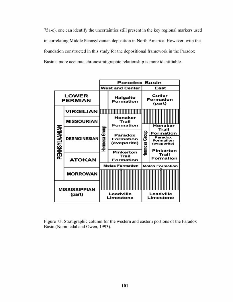
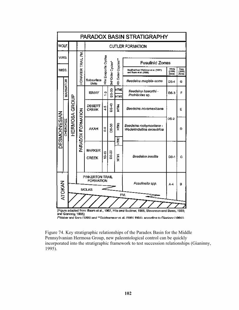
4.6 3-D model for Integration of 2-D Surfaces to Basin Distribution……….... 93 4.7 Stratigraphic Implications………………………………………………...100

v

CHAPTER 5. CONCLUSIONS ……………………….…………………………...105 REFERENCES………………………………………………………………………108

APPENDIX

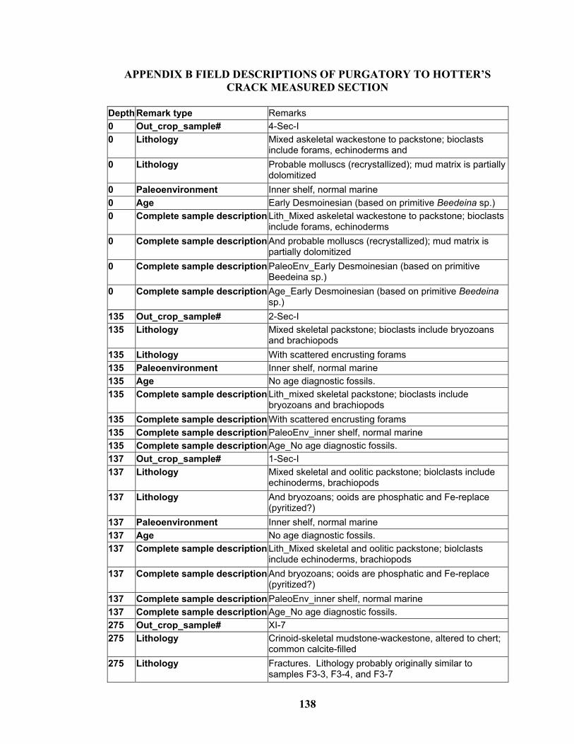
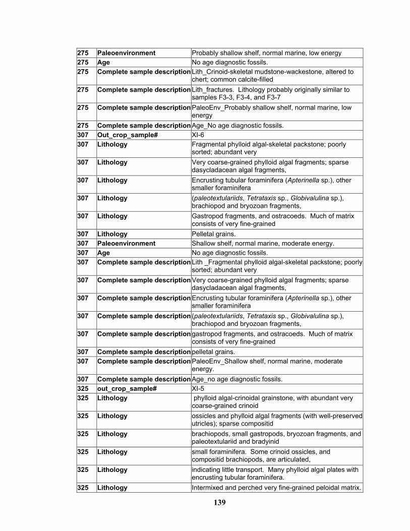
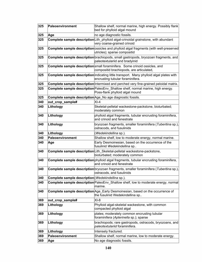
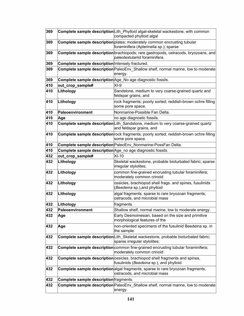
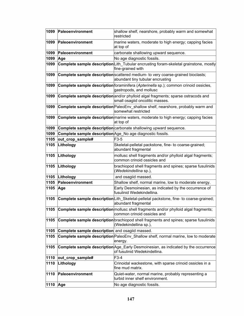
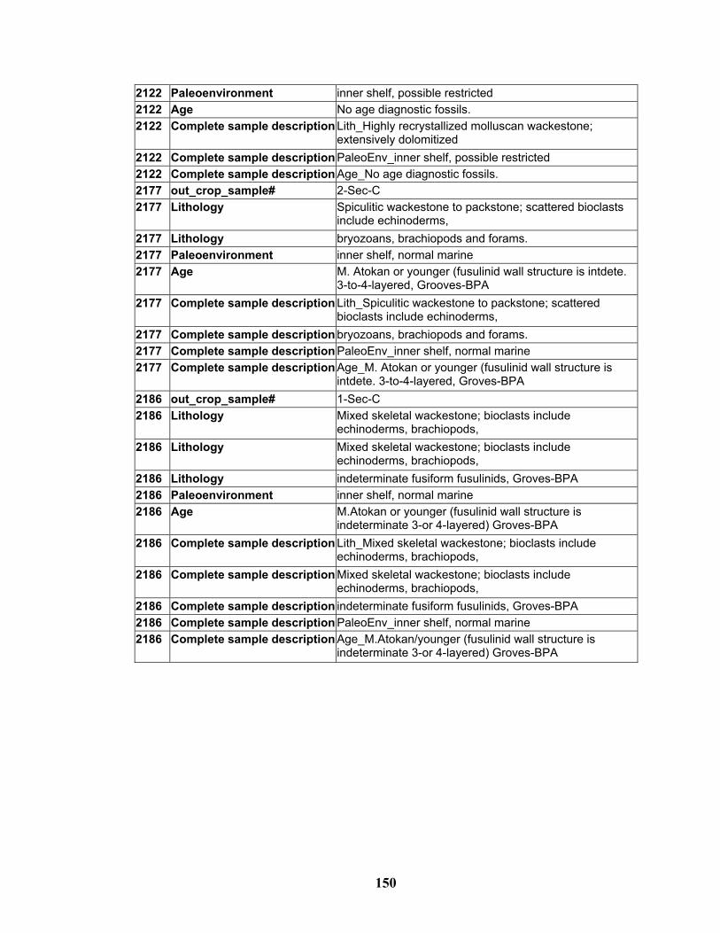
A STRATIGRAPHIC SECTION BIOSTRATIGRAPHY AND MICROFACIES…………………………………………………………113 B FIELD DESCRIPTIONS OF PURGATORY TO HOTTER’S CRACK MEASURED SECTION……………………….………………………...138 C FIELD MEASUREMENTS FROM OUTCROP OF SPECTRAL GAMMA-RAY RESPONSES………………………….…………….…..151 D NUCLEAR LOGGING TOOLS ...........................................…….……...154 E NNLAP WORKFLOW……………………..………………………....….158 F CROSS SECTION CONSTRUCTION CONTOURING WORKFLOW DESCRIPTION UTILIZING LANDMARK INTERPRETIVE APPLICATIONS STRATWORKS AND ZMAPPLUS……….……….165

VITA…………………………………………………………………………………180

vi

LIST OF TABLES

1. Traditional Desmoinesian fusulinid subzones and equivalent lithostratigraphic equivalents in the Mid-continent USA Region (Wahlman, 1999)…….…………….25

2. Descriptive comparison updated evaluation of Hermosa Mountain section compared to the Purgatory to Hotter’s Crack section…………………………………………..34

3. Lithology types with color code and numeric value for curve plotting.……...……..49 4. Sample number and depth from Hotter’s Crack to Purgatory measured section.….113

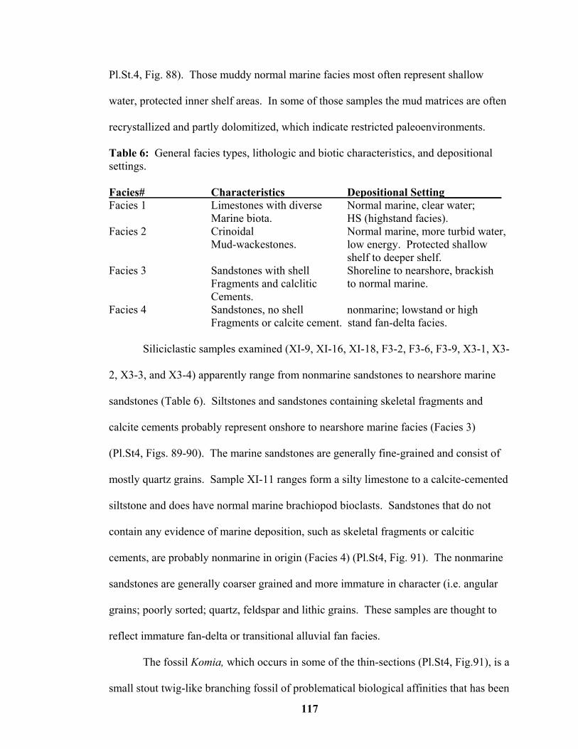
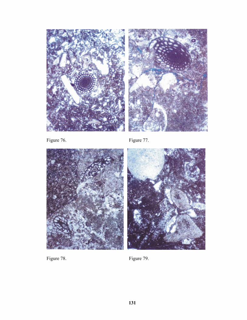
5. Listing of the occurrences of biostratigraphic diagnostic fossils in the thin-section samples examined, in descending stratigraphic order……………………………...116 6.General facies types, lithologic and biotic characteristics and depositional settings……………………………………………………………………………...117 7. Listing of samples from stratigraphic interval XI summary of lithologies, and paleoenvironmental interpretations ……………………………………….….……120

8. Listing of samples from stratigraphic interval F3 lithologies, and paleoenvironmental interpretations …………………………………………...…...121

vii

LIST OF FIGURES

1. General location map of study area with major regional tectonic elements………...2 2. Global continental reconstruction for the late Carboniferous………………….……3 3. The Four Corners region of the western United States showing the study area. Cross sections are highlighted and labeled ………………………………..………...7 4. Physiographic features of the study area…………………………………………….9

5. Stratigraphic column for study area………………………………………………..10

6. Structural Schematic diagram across the southern Paradox Basin..……….………12

7. Structural elements affecting Pennsylvanian deposition………………………..….13

8. Location map of key stratigraphic outcrop sections with surface geology in the Animas Valley area………………………………………………………………...16

9. Preserved Pennsylvanian age strata and inferred physiographic features in the Four Corners Area……………………………………………………...…...18 10. Schematic of Eastern Paradox Basin Salt Anticline development………………....19 11. Preserved Permian age strata and inferred physiographic features in the Four

Corners Area…………………………………………………………………….…23 12. Paradox Basin stratigraphy and key biostratigraphic zonations…………………....26 . 13. Location map Durango to Quray, Colorado…………………….……………….....29 14. Hotter’s Crack to Purgatory measured section location .…………………………..30 15. Upper Hotter’s Crack measured section with lithnum curve representing numerical

value of lithology…………………………………...…………………………..32 16. Upper Hotter’s Crack measured section segments G,H, and I…………………..…33 17. Field picture of measured section at Hotter’s Crack with lithology description sand

spectral gamma-ray...………………………………………………………………33

18. Lower section of Hermosa Group just above the Pinkerton Formation contact…...36

viii

19. Outcrop spectral gamma-ray measurements and lithology descriptions for full

measured section description ...……………………………………………………38 20. Outcrop total gamma-ray (GR) measurements by color-code lithology type, see

Table 3 for color bar-lithology reference…………………………………………..38 21. Total Uranium (u) Total Potassium (k) cross correlation.…………………………39 22. Total Gamma (t) versus Total Potassium (k) count from Scintillometer

measurements with color lithologies ………………………………………………40 23. Crossplot of lithology type (y) versus total gamma-ray (x)from wireline

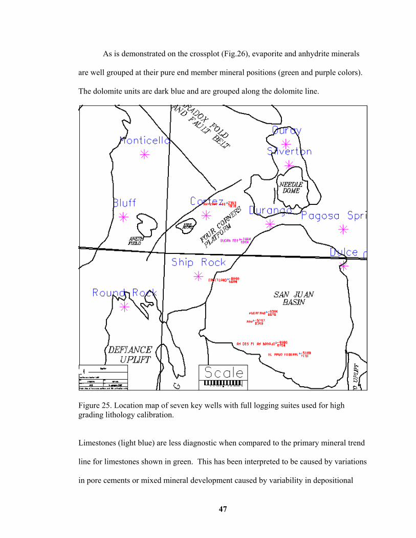
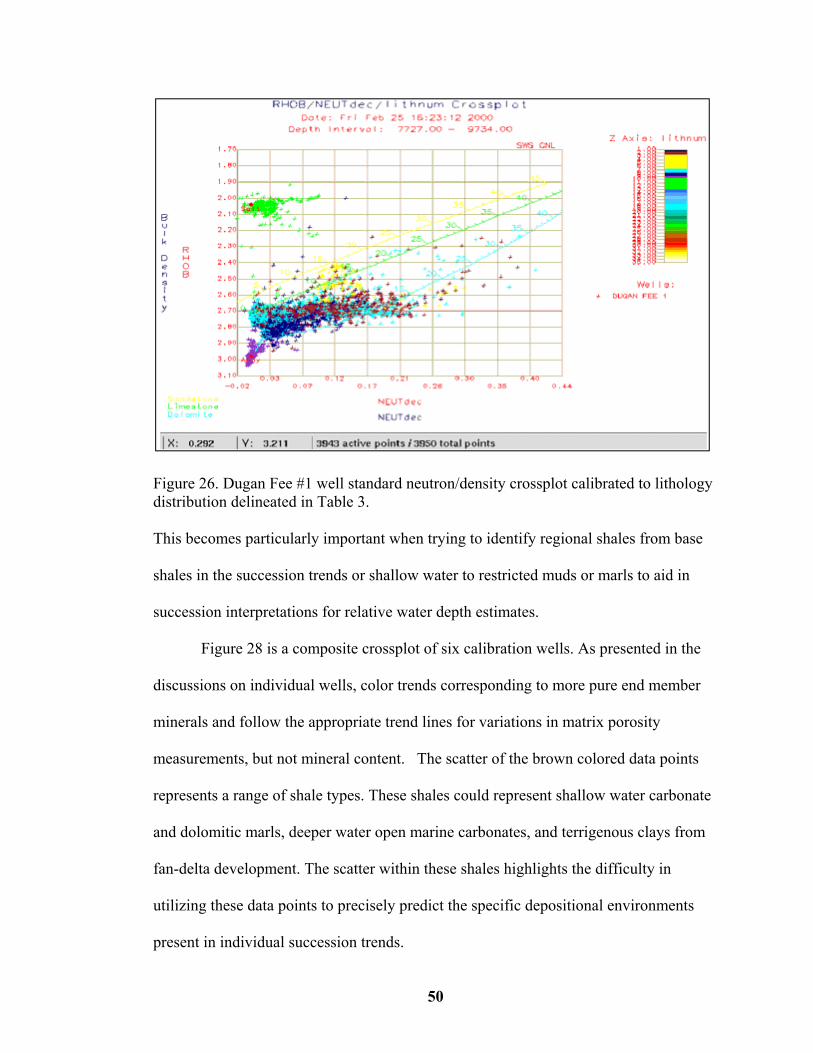
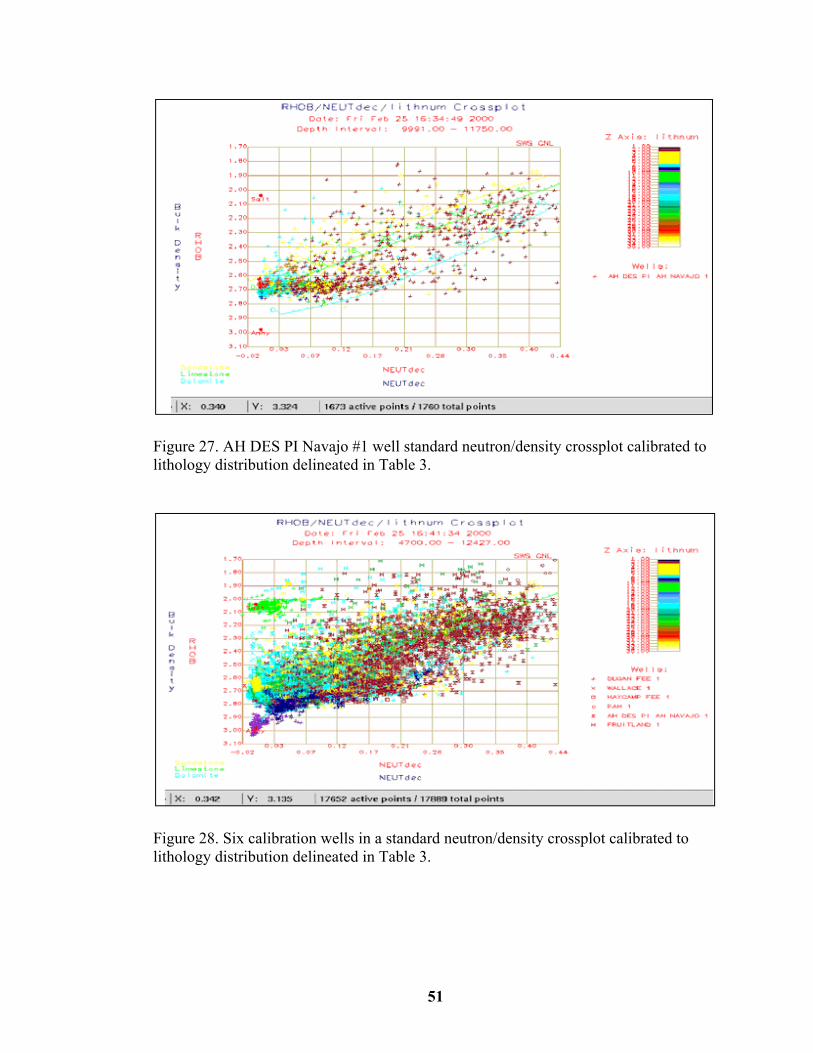
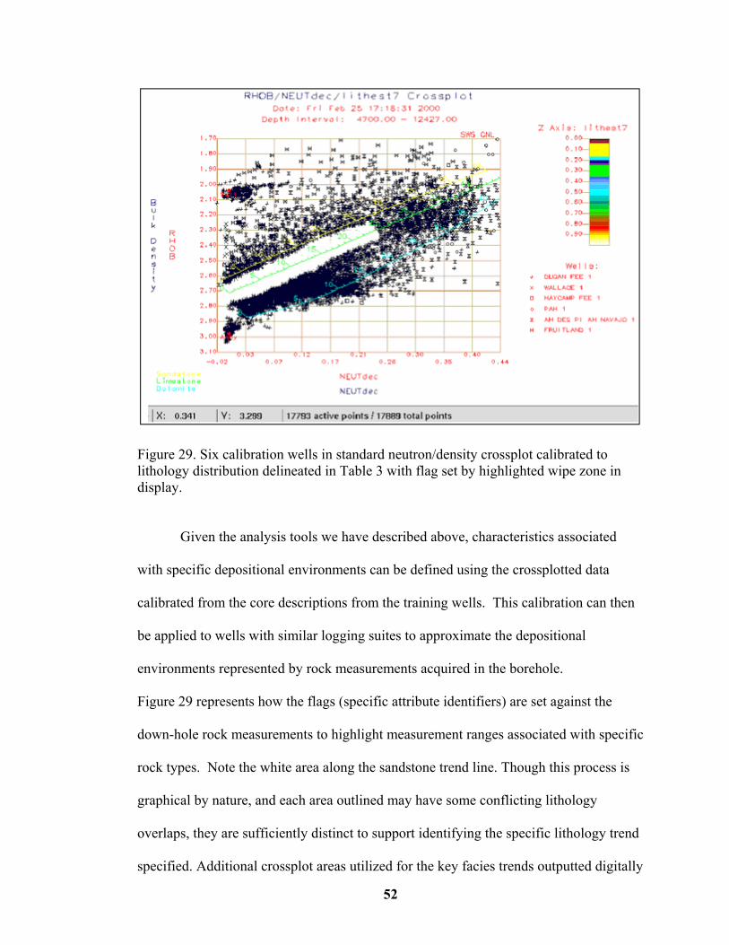
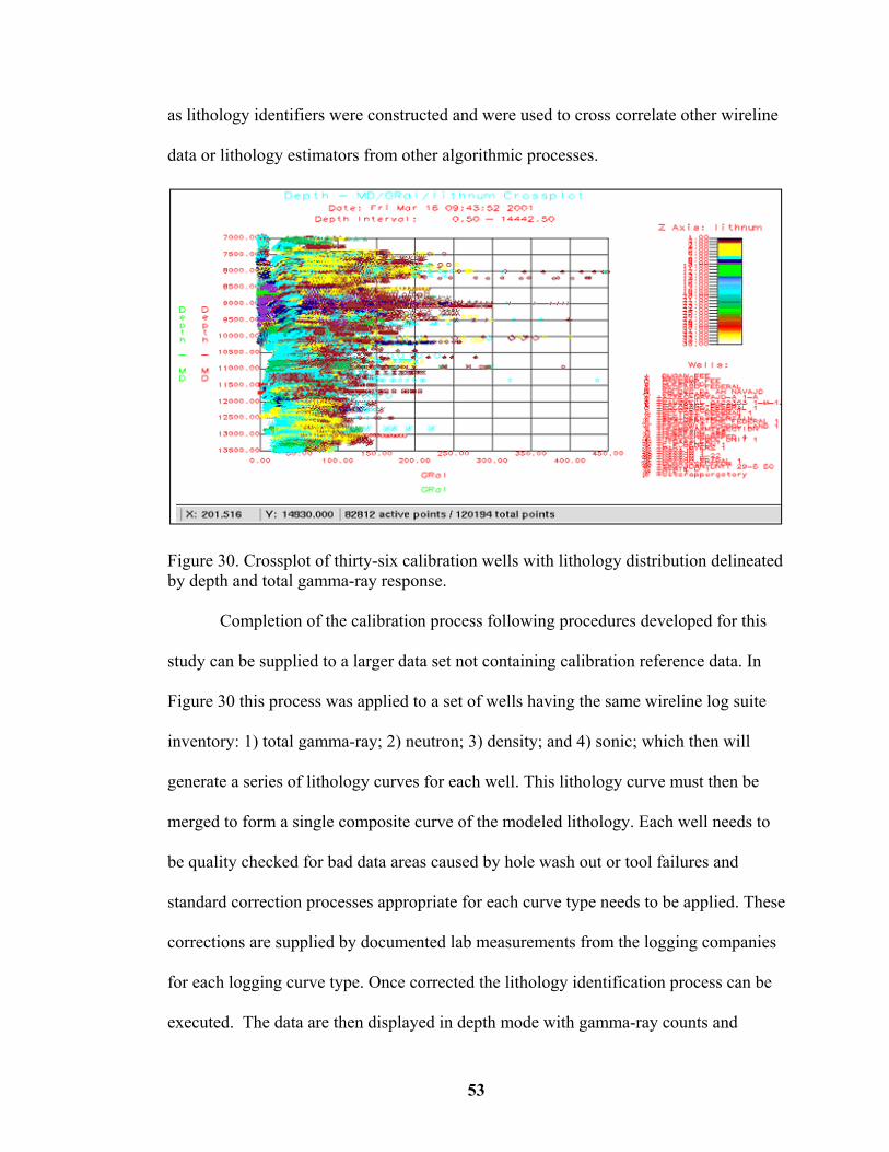
measurements for 36 calibration wells ………………………………………….…40 24. Location map of 36 lithology calibration wells……………………………………46 25. Location map of seven key wells with full logging suites used for high grading lithology calibration………………………………………………………………..47 26. Dugan Fee #1 well standard neutron/density crossplot…………………………....50 27. Ah Des Pi Ah Navajo #1well neutron/density standard crossplot………………....51 28. Six calibration wells in a standard neutron/density crossplot calibrated to lithology distribution ……………………………………………………………....51 29. Six calibration wells in standard neutron/density crossplot calibrated to

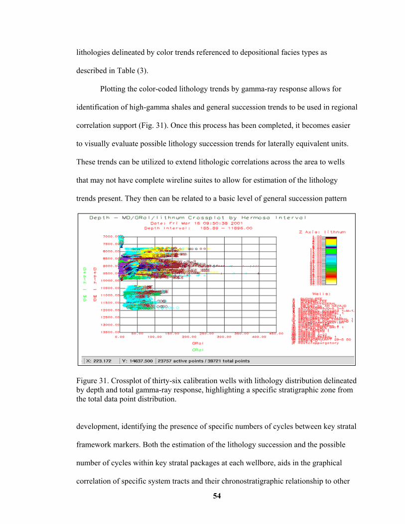
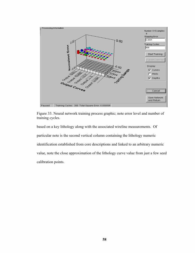
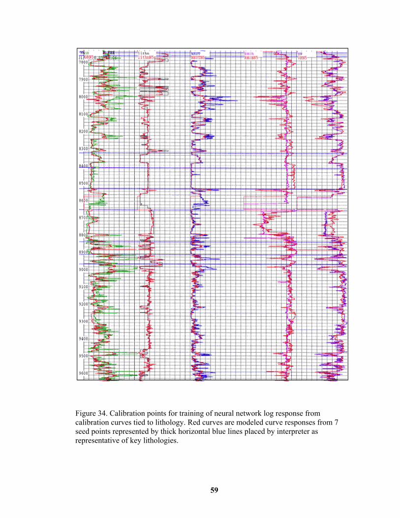
lithology distribution …………………………………………………...…………52 30. Cross plot of thirty-six calibration wells with lithology distribution delineated depth and total gamma-ray response………………………………………….……53 31. Crossplot of thirty-six calibration wells with lithology distribution delineated by depth and total gamma-ray response, highlighting a specific stratigraphic zone from the total data point distribution……………………………………………...……...54 32. Back propagation neural node model……………………………………………....56 33. Neural network training process graphic……………….………………………….58 34. Calibration points for training of neural network log response from calibration curves tied to lithology.…………………………………………………………....59 35. For the Dugan Fee #1 well lithology prediction (lithesta) versus lithology ground truth from core (lithnum) lithology types………………………………………….61

ix

36. For the Dugan Fee #1 well lithology prediction (lithesta) versus lithology ground

truth from core (lithnum) with color distribution representing specific lithology types………………………………………………………………………………..61

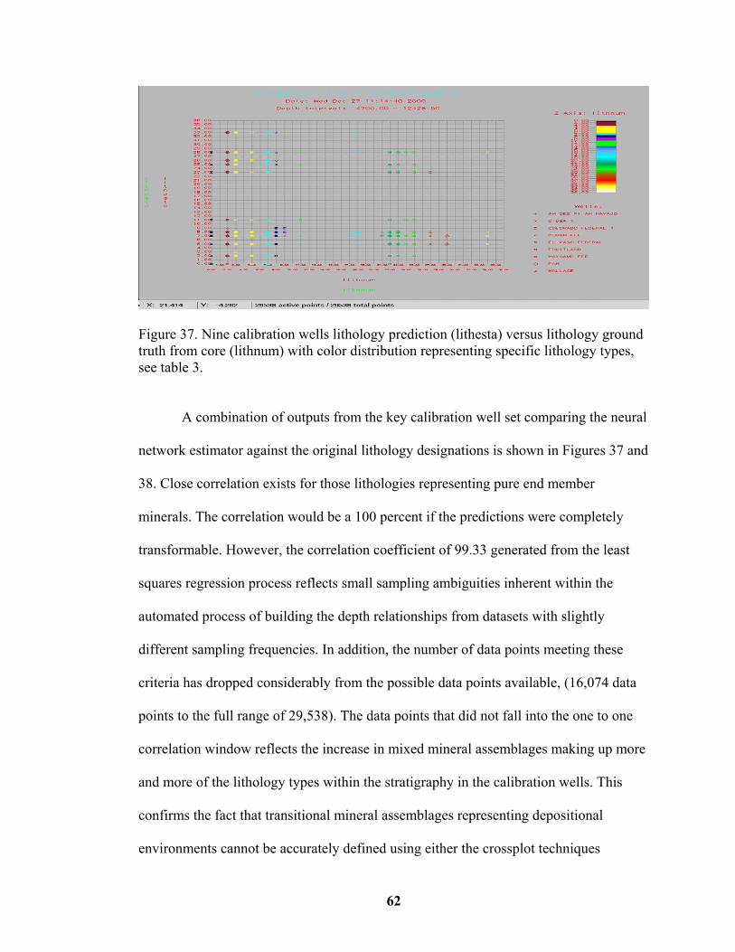
37. Nine calibration wells lithology prediction (lithesta) versus lithology ground truth from core (lithnum) with color distribution representing specific

lithology types……………………………………………………………………...62

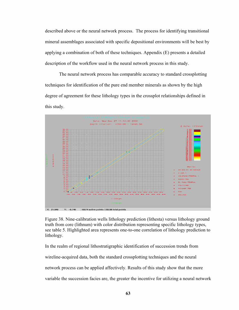
38. Nine calibration wells lithology prediction (lithesta) versus lithology ground truth from core (lithnum) with color distribution representing specific lithology types………………………………………………………………………….…….63

39. Regional structural cross section surface correlations from Ouray, Colorado to

Mexican Hat, Utah ………………………………………………………………...67

40. Location map for key cross sections constructed and wells…..…………………...67

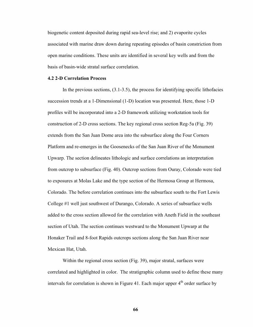
41. Definition of the stratigraphic column defining specific correlation surface……....68

42. Lithology successions across the Desert Creek and Ismay intervals Dugan Fee #1 well……………………………………………………………………..…………..69

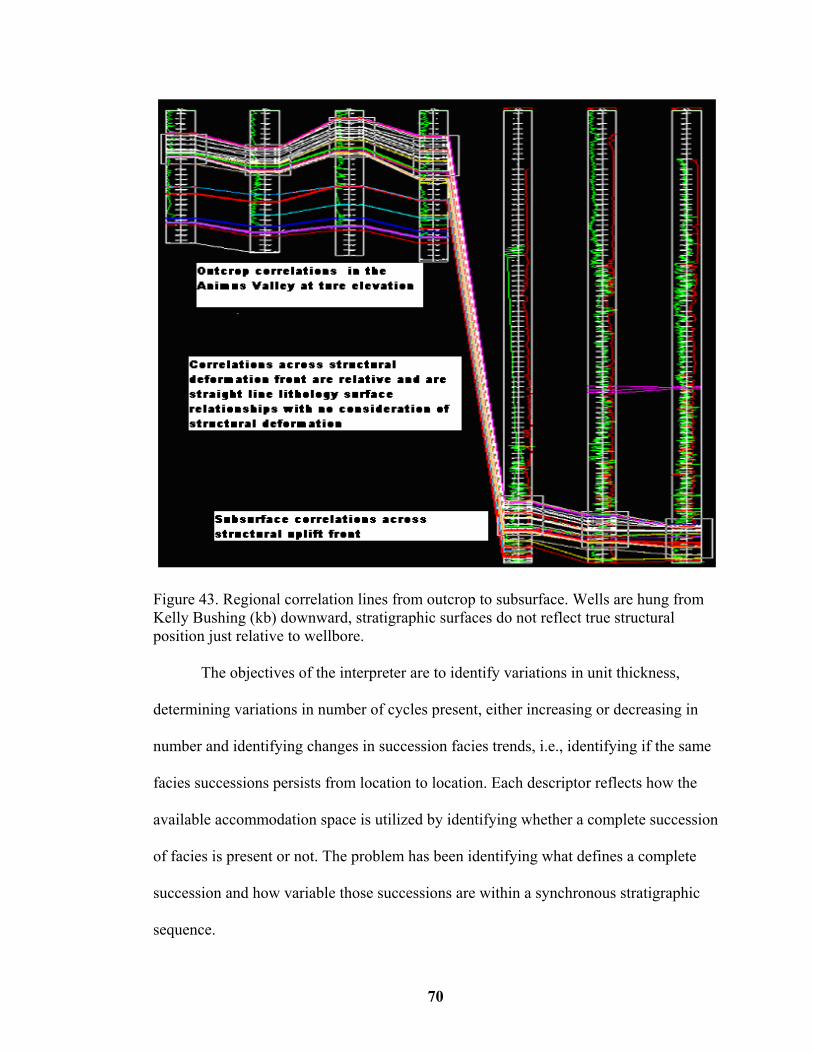
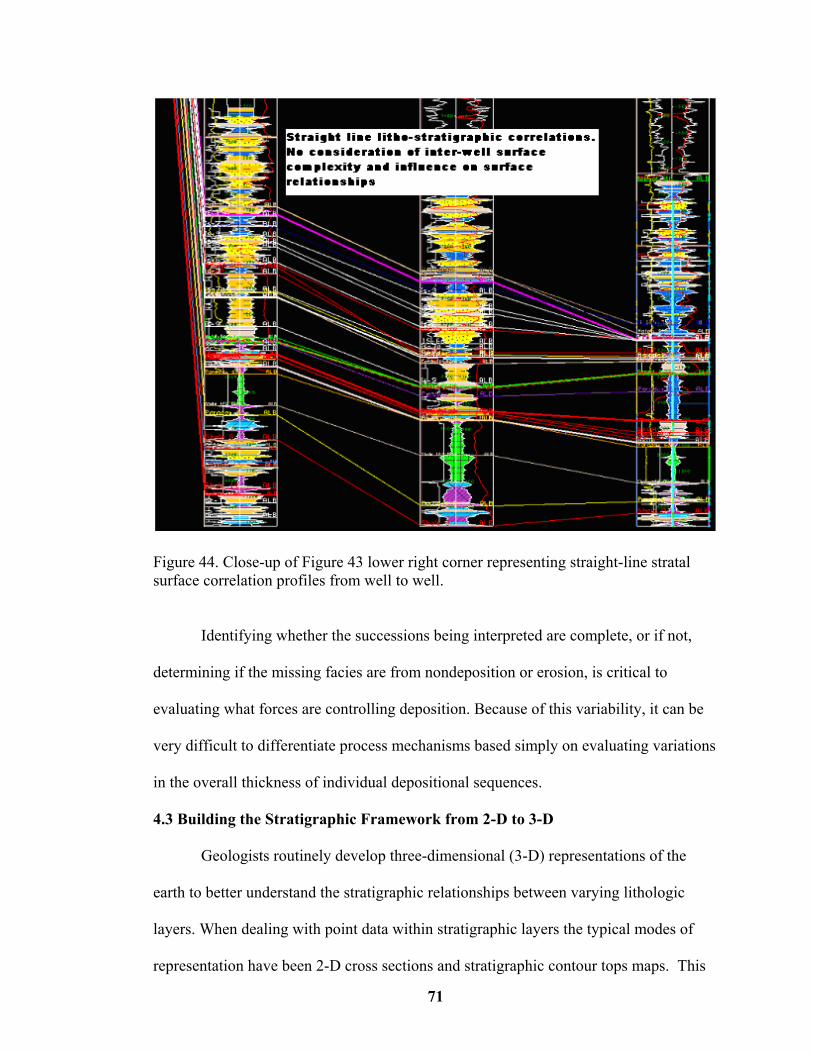
43. Regional correlation lines from outcrop to subsurface ………...……………….....70 44. Close-up of Figure 43 lower right corner representing straight-line stratal

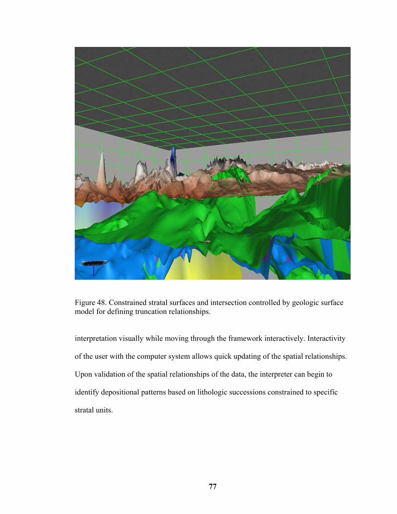
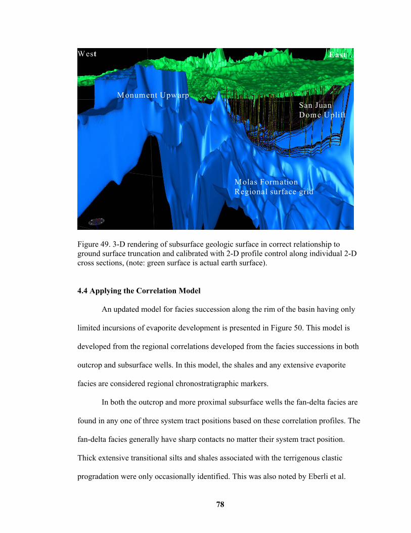
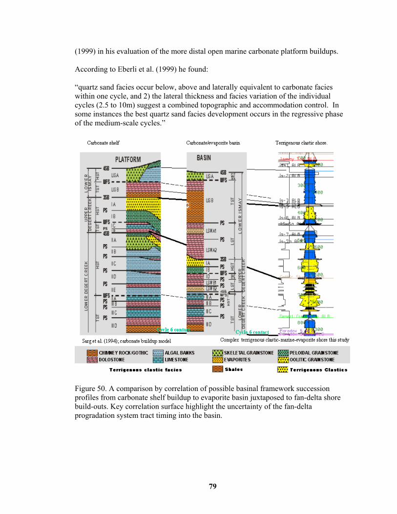
surface correlation profiles from well to well………………………...……….…..71 45. Map level with large grid radius of (2500m) …………………………………..…75 46. Map level with smaller grid radius of (300m) ……………………………….…..75 47. Un-constrained stratal grid surfaces………………………….………………….....76 48. Constrained stratal surfaces and intersections…………………….…………….….77 49. 3-D rendering of subsurface geologic surfaces………………………….………....78 50. Succession profiles from carbonate shelf buildup to evaporite basin

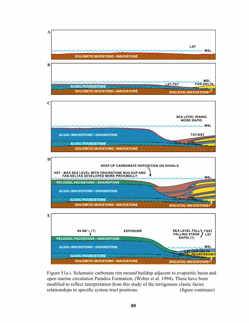
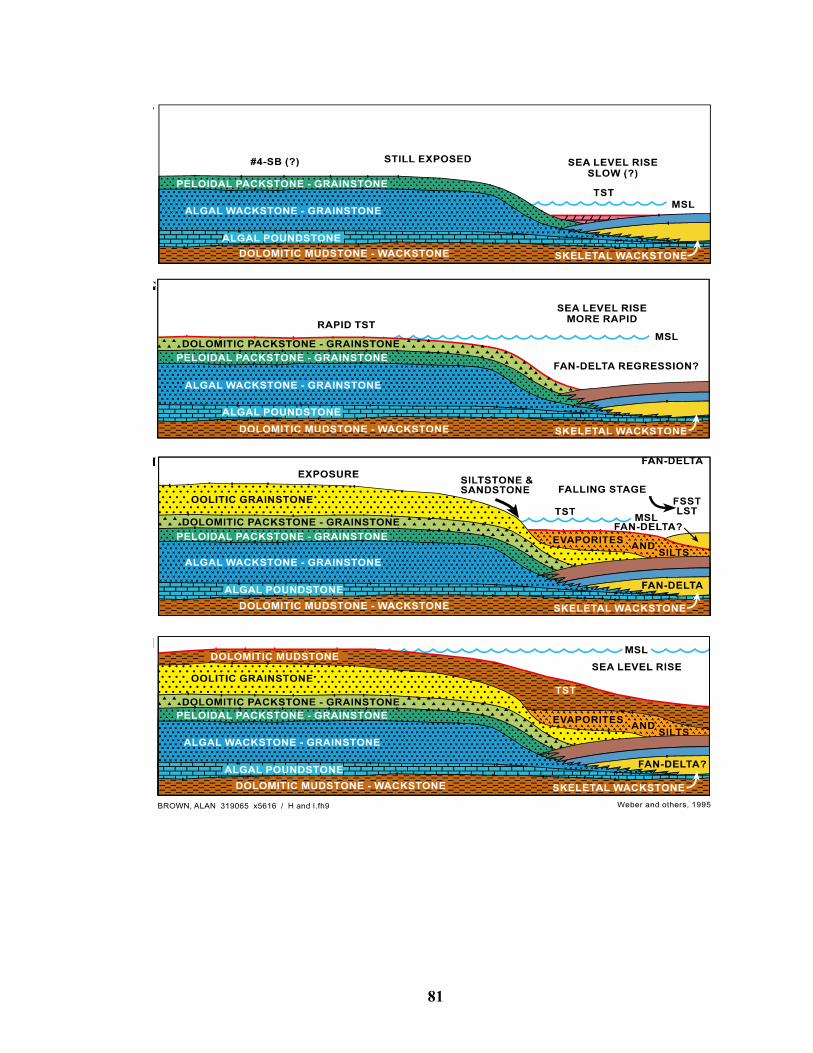
juxtaposed to fan-delta shore build-outs………………………………………..…79 51a-i. Schematic carbonate rim mound buildup adjacent to evaporitic basin and

open marine circulation Paradox Formation………………………………….....80

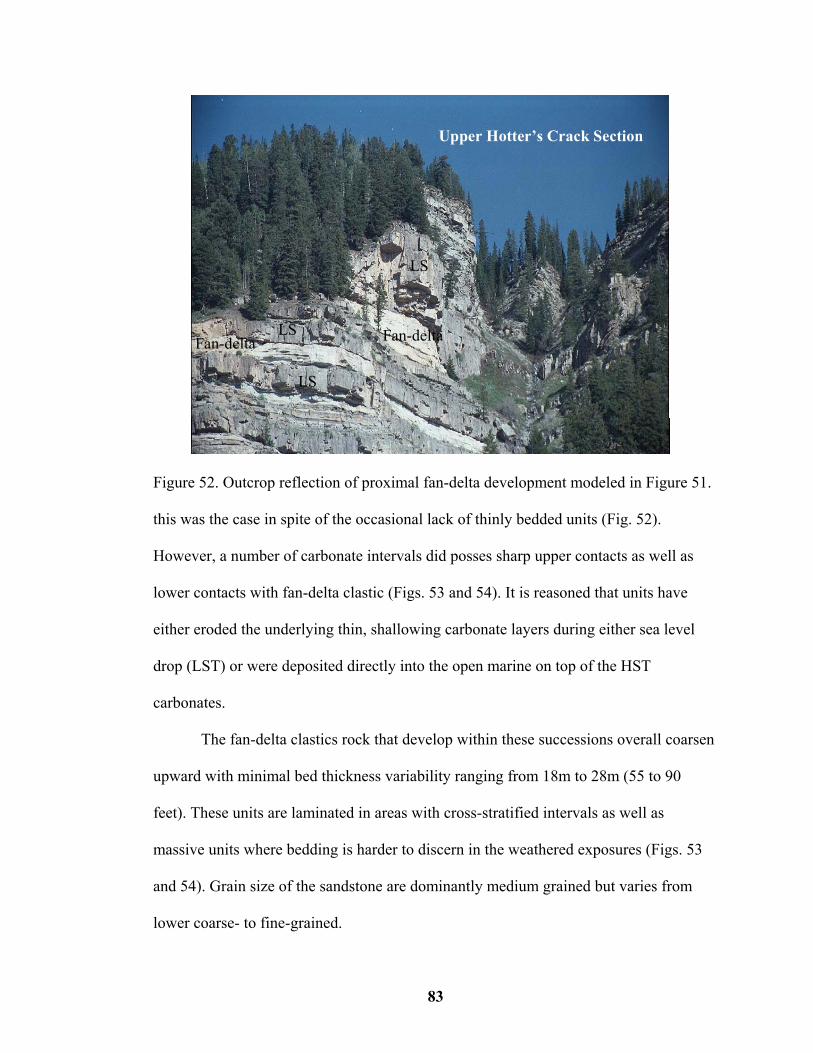
52. Outcrop reflection of proximal fan-delta development………………………….…83

x

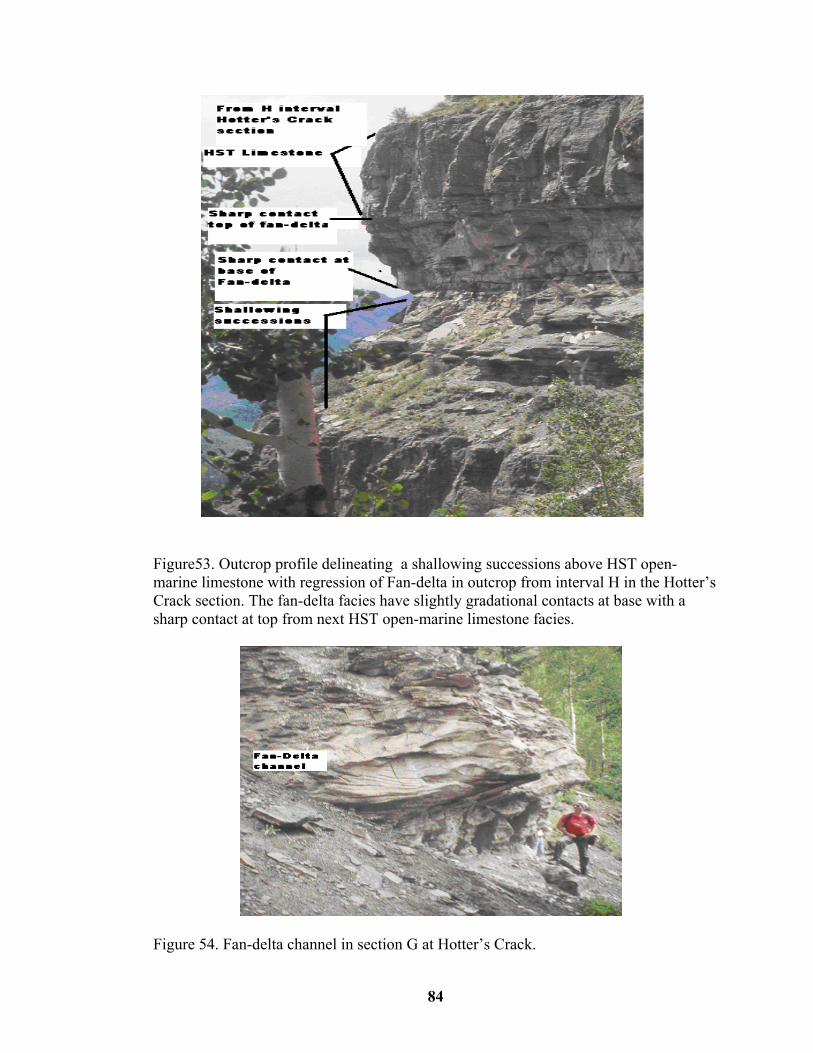
53. Outcrop profile delineation a shallowing succession…………………..……….....84

54. Fan-delta channel in section G at Hotter’s Crack………………………..………..84

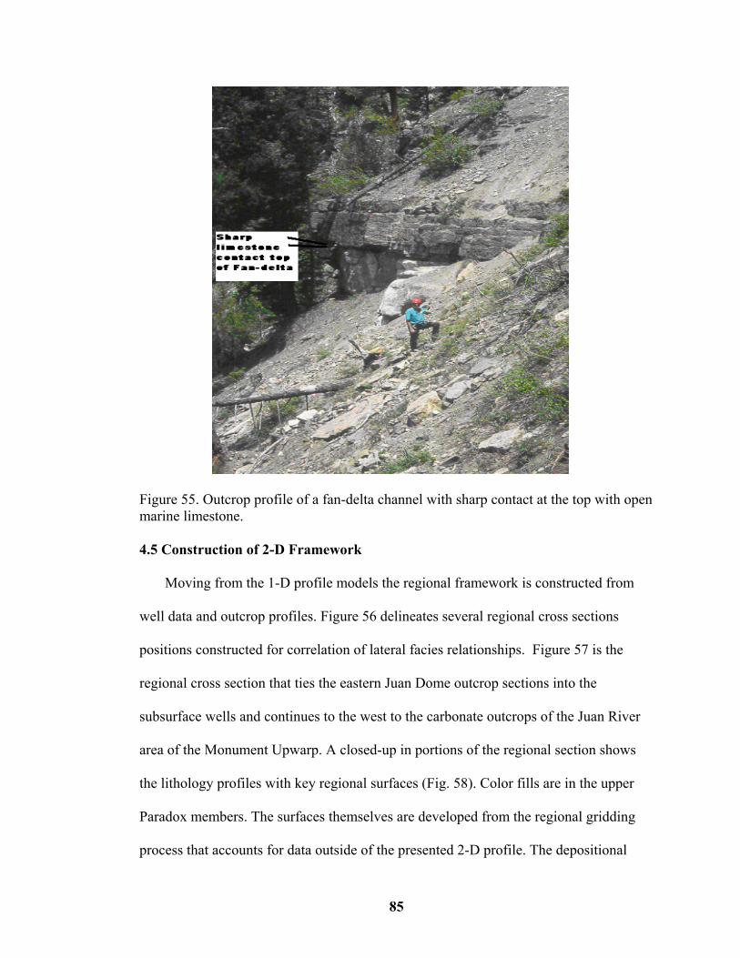
55. Outcrop profile of a fan-delta channel……………………………………………..85 56. Regional base map with location of cross section and wells……………..……..…86 57. Regional cross section from the San Juan Dome Outcrop ties to subsurface

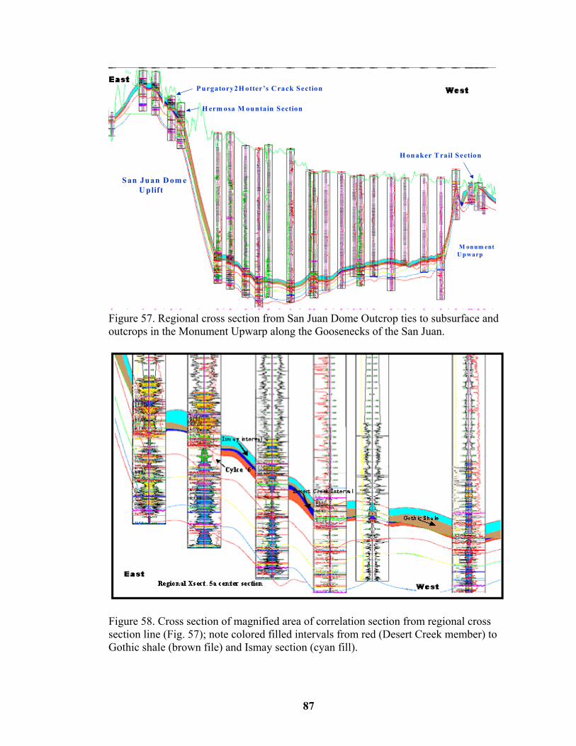
and outcrop ties in the Monument Upwarp area……………………………..…….87 58. Cross section of magnified area of correlation section from cross section

line (Fig 57)……………………………………………………………..…………87

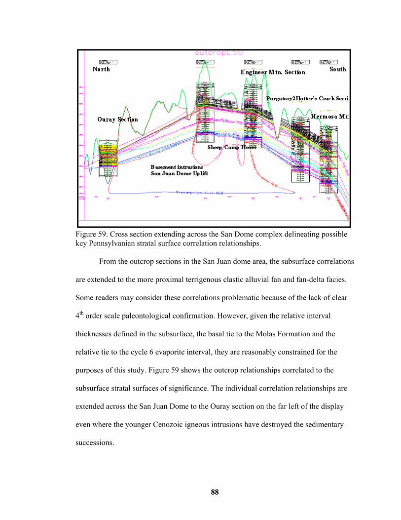
59. Cross section extending across the San Dome complex delineating possible key Pennsylvanian stratal surface correlation relationships……..……….………..88

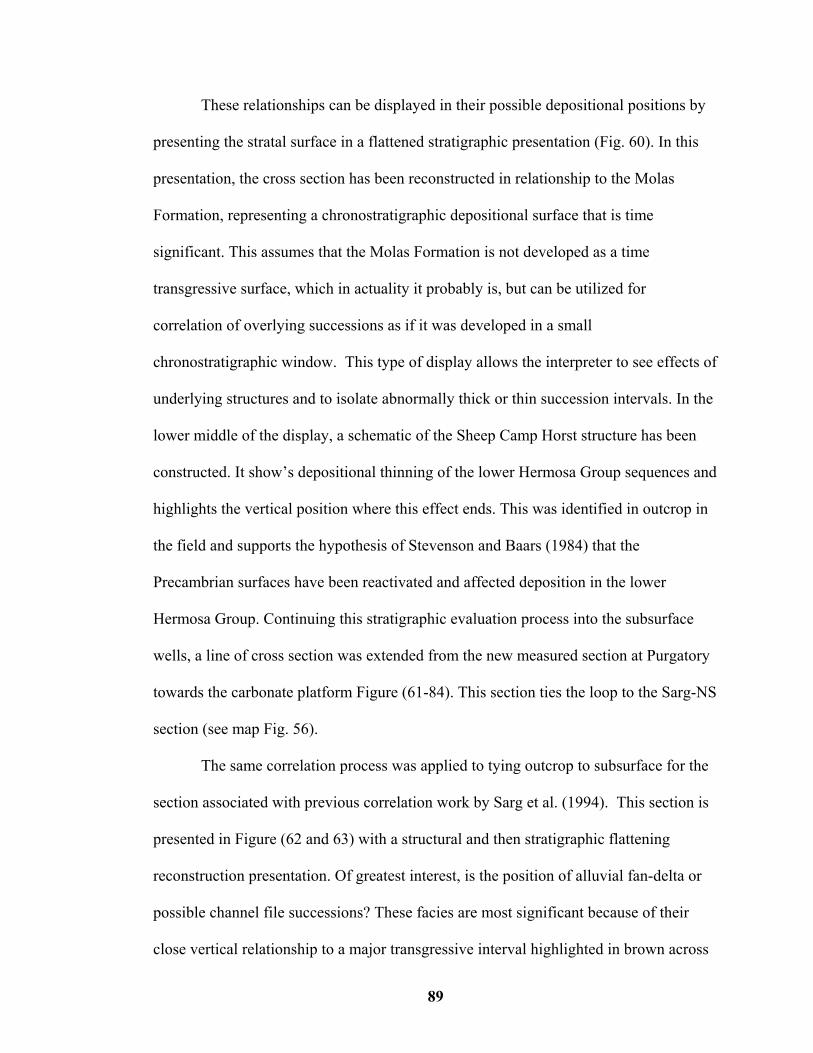
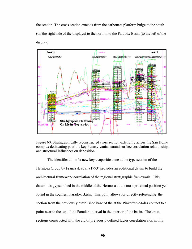
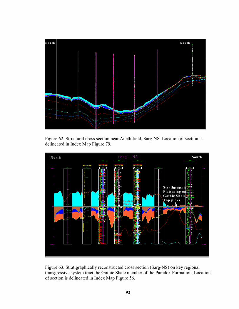
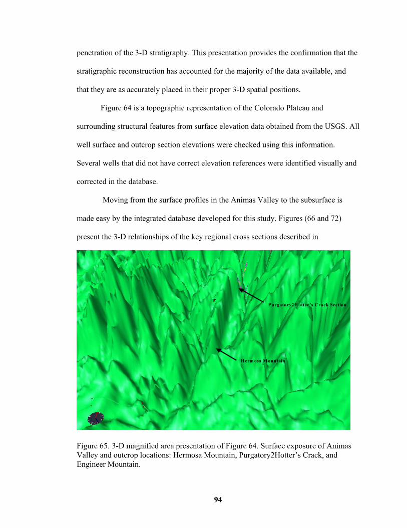
60. Stratigraphically reconstructed cross section extending across the San Juan Dome.90 61. Structural cross section ties from Purgatory measured section extending west- southwest ………..………………………………………………………………...91 62. Structural cross section near Aneth field, cross section line (Sarg-NS)……………92 63. Stratigraphically reconstructed cross section (Sarg-NS) datumed on Gothic Shale.92 64. 3-D of surface topography………………………..………………………………..93 65. 3-D magnified area of Figure 64………………………………………………...…94

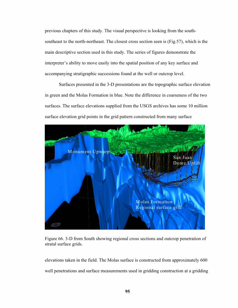
66. 3-D from south showing regional cross sections and outcrop penetration of stratal surface from gridded data………………………………………………….……....95

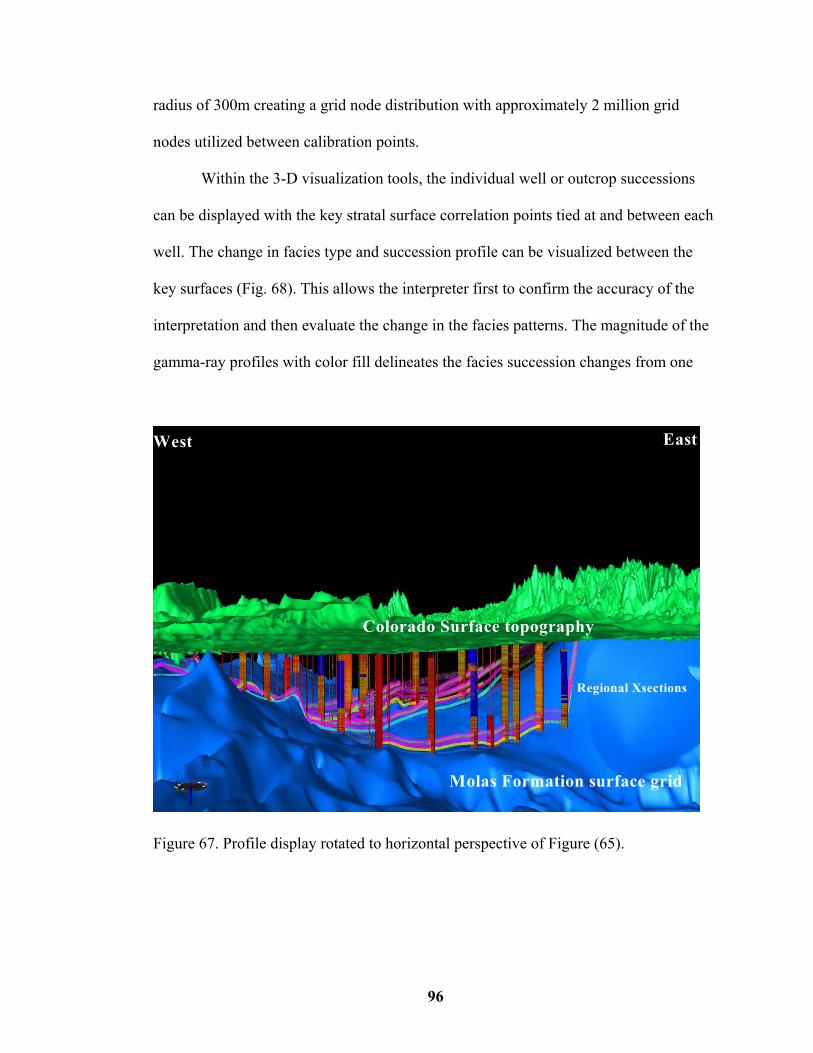
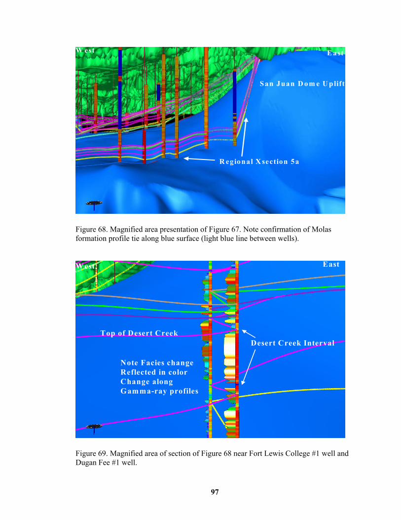
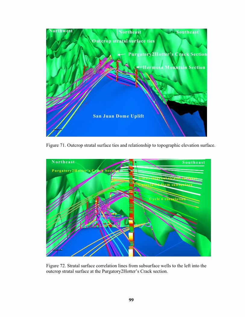
67. Profile display rotated to horizontal perspective of Figure 65…...…………..…….96 68. Magnified area presentation of Fig. (67)………………………..……….………...97 69. Magnified area section of Fig. (68) near Fort Lewis College #1 well and Dugan Fee #1 well……………………………………………………………….....97 70. Stratal surface ties from subsurface wells along key cross sections to the outcrops measured in the San Juan Dome area……………………………………………....98 71. Outcrop stratal surface ties and relationship to topographic elevation surface…….99

xi

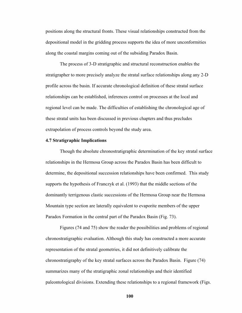
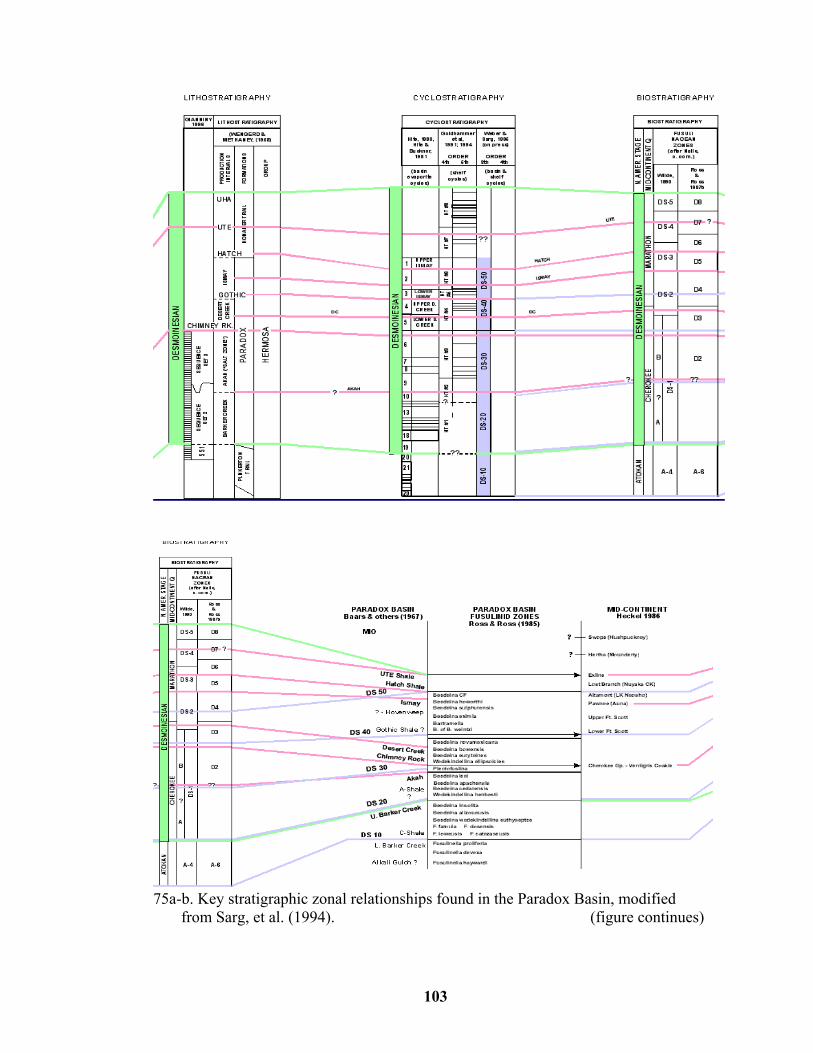
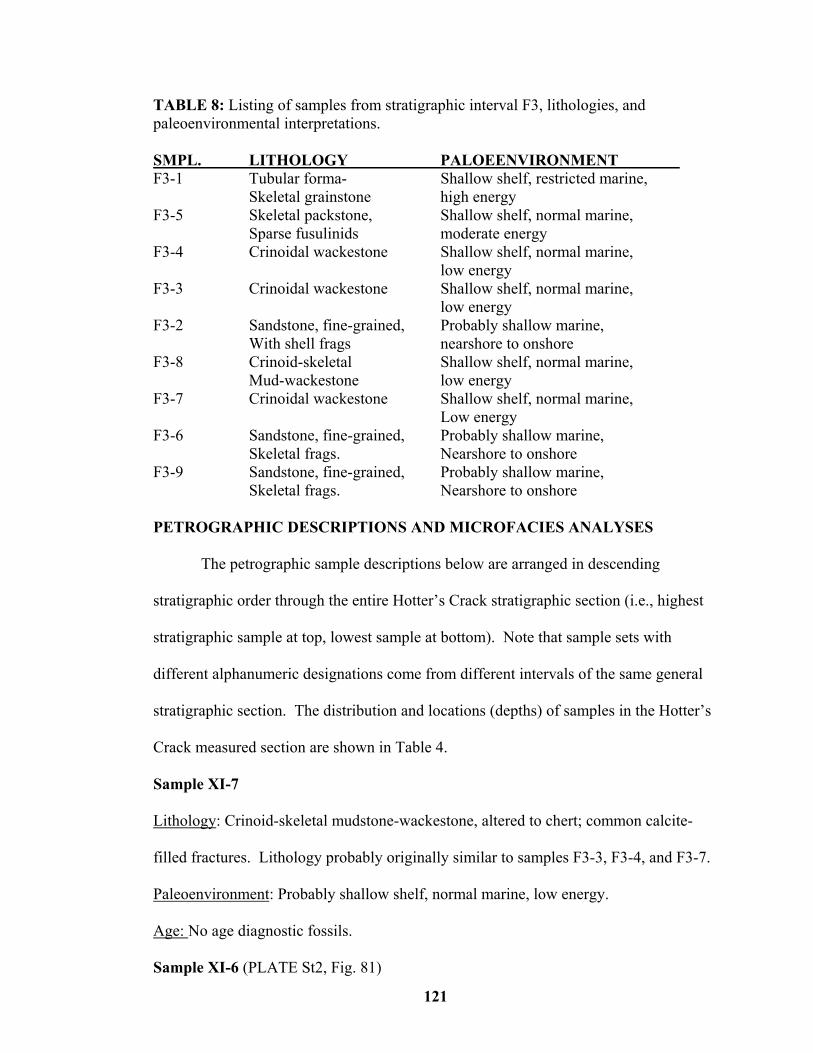
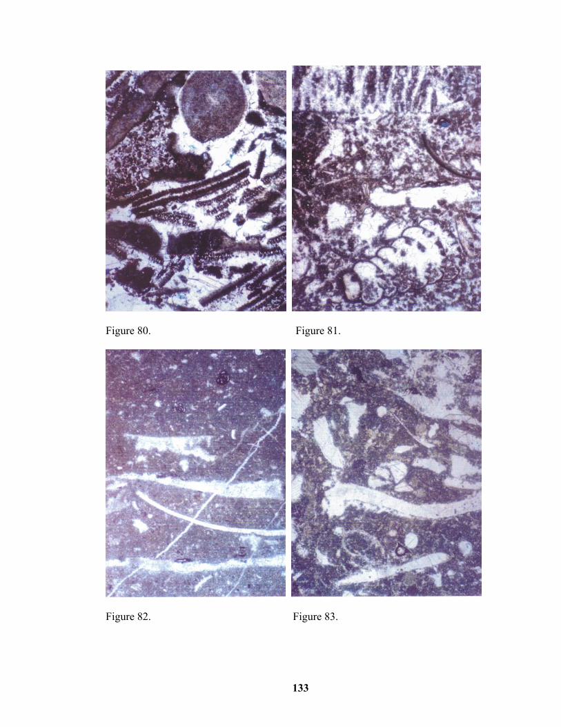
72. Stratal surface correlation lines from subsurface wells on left into the outcrop stratal surface at the Purgatory2Hotter’s Crack section…………………...……….99 73. Stratigraphic column for the western and eastern portions of the Paradox Basin………………………………………………………...…………………….101 74. Key stratigraphic relationships of the Paradox Basin ……………………………102 75a-b. Key stratigraphic zonal relationships found in the Paradox Basin, modified from Sarg, et al. (1994)…………………………………………………………...103 76. Sample F3-5……………………………………………………………………….131 77. Sample XI-4……………………………………………………………………….131 78. Sample XI-10……………………………………………………………………...131 79. Sample XI-13……………………………………………………………………...131 80. Sample XI-5……………………………………………………………………….133 81. Sample XI-6……………………………………………………………………….133 82. Sample XI-8……………………………………………………………………….133 83. Sample XI-15……………………………………………………………………...133 84. Sample F3-1……………………………………………………………………….135 85. Sample XI-14……………………………………………………………………...135 86. Sample XI-17……………………………………………………………………...135 87. Sample F3-3……………………………………………………………………….135 88. Sample F3-7……………………………………………………………………….137 89. Sample XI-11……………………………………………………………………...137 90. Sample F3-2……………………………………………………………………….137 91. Sample XI-18……………………………………………………………………...137

xii

ABSTRACT

Pennsylvanian (Desmoinesian) sedimentary rocks within the Paradox Basin Four

Corners area of the western United States afford a unique opportunity to study the

development of sedimentary successions in a complex marine to nonmarine

depositional setting. The close association of thick intervals of nonmarine fan-delta

facies adjacent to and in time equivalent position to marine carbonate-evaporite facies

suggests complex relationships between the factors affecting deposition. Development

of an effective scheme to differentiate the depositional signatures from within these

sedimentary successions is the primary goal of this study. To achieve this goal, two

objectives were pursued. The first was to calibrate the diverse range of rock-types in

the Hermosa Group to in-situ wellbore measurements. To facilitate this process, a

neural network evaluation procedure coupled with standard petrophysical evaluation

techniques were employed to aid in facies succession prediction and lateral facies

correlation. This process proved to be as accurate as standard wireline analysis

procedures and was able to account for variations not as detectable in conventional

scheme. The second objective was to correlate the stratigraphy of the Hermosa Group

from outcrops of the Animas Valley to the subsurface along the southern Paradox

Basin. The key to understanding the depositional sequences within the Middle

Pennsylvanian section is to determine spatial and temporal relationships between the

evaporites and black-shale deposits associated with carbonate algal mound buildups and

juxtaposed terrigenous clastic fan-delta depositional facies. Once the relationships of

these facies successions are delineated, then a three dimensional architectural

framework can be manipulated to examine all possible lateral facies successions. By

xiii

utilizing these analyses, several members of the Paradox Formation were shown to be

laterally equivalent and physically continuous with parts of the previously designated

undifferentiated Honaker Trail Formation of the San Juan Dome region.

The study required a rigorous integration process utilizing a digital workstation

environment combining large and more diverse datasets than previously utilized for

improved correlation control. Techniques for evaluation of facies successions involved

core (42), subsurface wells (4000+), and measured sections (12+) were employed.

1

CHAPTER 1. INTRODUCTION

1.1 Overview of Geologic Setting and Objectives

Baars (1972) describes the area at the intersection of the states of Colorado, Utah,

Arizona, and New Mexico as “Red Rock Country” for the great exposures of red-brown

cliffs and canyons (Fig. 1). This area is commonly referred to as the Four Corners

Region of the Colorado Plateau. Within these canyon systems exist some of the most

striking examples of cyclic sedimentary deposition involving a complex

interrelationship between open marine, evaporitic and siliciclastic deposition. These

cycles have been studied extensively over the years in an attempt to understand what

sedimentary processes controlled their depositional patterns (Roth, 1934; Wengerd and

Strickland, 1954: Spoelhof, 1974; Stevenson and Baars, 1984; Goldhammer et al., 1991

and 1994). In particular, these sedimentary successions are type examples showing of

the dominance of eustasy on depositional architecture. Many factors, however, control

the process of sedimentation; eustasy, tectonics, climate, and sediment supply are some

of the most important ones. Understanding the interdependencies of these depositional

processes on controlling depositional successions is of fundamental interest to

geologists.

The stratigraphic interval of interest in this study is the Middle Pennsylvanian

(Desmoinesian) Hermosa Group. It is composed of a series of coalescing marine

carbonates, evaporites, and terrigenous clastic deposits formed in a shallow

intercontinental sea extending over the Four Corners Region (Stevenson and Baars,

1984). This sea occupied an equatorial setting between 5 degrees north and south

latitude (Fig 2) in an extremely arid climate that accumulated over 2 Kilometers (+7000

2

feet) of evaporitic sediments (Baars, 1972). These marine sedimentary rocks form a

series of stacked successions that are punctuated by many unconformities and

regionally extensive shales. The regionally extensive shales are considered to have been

Figure 1. General location map of study area showing major tectonic elements. Regionally referred to as the Four Corners Region of Western USA, modified from Wood (1987). Modified from Houch (1998); deposited during rapid marine transgressions and coincided with many short duration

repetitive rises in sea level approximately 100,000 to 400,000 years in length

(Goldhammer et al., 1991 and 1994). These marine rocks interfinger laterally with non-

marine terrigenous clastic rocks adjacent to the western flank of the ancestral

Uncompahgre Uplift (Stevenson and Baars, 1984). The product of this depositional

3

system is the Hermosa Group of the Paradox Basin (Hite, 1960; Peterson and Hite

1969; and, Hite and Buckner, 1981).

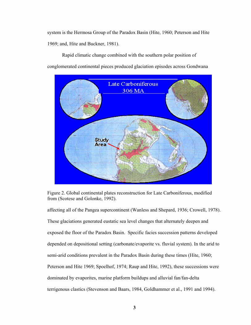
Rapid climatic change combined with the southern polar position of

conglomerated continental pieces produced glaciation episodes across Gondwana

Figure 2. Global continental plates reconstruction for Late Carboniferous, modified from (Scotese and Golonke, 1992). affecting all of the Pangea supercontinent (Wanless and Shepard, 1936; Crowell, 1978).

These glaciations generated eustatic sea level changes that alternately deepen and

exposed the floor of the Paradox Basin. Specific facies succession patterns developed

depended on depositional setting (carbonate/evaporite vs. fluvial system). In the arid to

semi-arid conditions prevalent in the Paradox Basin during these times (Hite, 1960;

Peterson and Hite 1969; Spoelhof, 1974; Raup and Hite, 1992), these successions were

dominated by evaporites, marine platform buildups and alluvial fan/fan-delta

terrigenous clastics (Stevenson and Baars, 1984, Goldhammer et al., 1991 and 1994).

4

In the more humid climate in the Appalachian Basin these successions are fluvially

dominated with coal development (Donaldson et al., 1979; Brown, 1982). Each area

shows a succession profile with a Punctuated Aggradational Cycle (PAC) including a

shallowing-upward cycle separated by surfaces marked by abrupt changes to deeper

facies that take on different characteristics depending on the climatic conditions of the

area both reflecting the worldwide glaciations that develop (Goodwin and Anderson,

1985).

The many cycles and unconformities found throughout the area indicate that the

shallow sea of the Paradox Basin responded to slight fluctuations in sea level. These

Pennsylvanian age cycles are considered to have developed in response to changing

climatic conditions dominated by glacial events over the southern hemisphere portion of

Pangea (Fig. 2; Wanless and Shepard, 1936; Crowell, 1978; Goldhammer et al., 1991).

The PACs are thought to represent successive stacking of repeated depositional facies

that coarsen or shallow upwards and are abruptly terminated by a definable stratigraphic

surface, either an exposure surface or abrupt shallowing or deepening sequence at the

parasequence level. Research reported here suggests that these repetitions may occur

more often over a given, relatively short geologic time frame than at most other times in

geologic past. It will be shown below that the surfaces that define these changes from

one succession to another are roughly correlateable globally. This depositional pattern

dominated Pennsylvanian sedimentation all over the globe but were manifested locally

depending on local tectonics, climate, sediment source, and depositional environment.

1.2 Goals and Objectives

The goal of this study is to define an effective methodology for more precisely

defining the relationship between cyclic signatures in a depositional environment that

5

juxtaposes facies successions from marine, evaporite and terrigenous fan-delta

depositional processes. To accomplish this, two objectives needed to be attained: 1)

development of methodologies to acquire and integrate pertinent lithology data from

outcrop and/or core using subsurface wireline information; and 2) to apply these

methodologies to evaluate the predictability of facies relationships in the Pennsylvanian

system and correlate their relationships from outcrop to subsurface across the southern

Paradox Basin where the section is affected by both eustasy and tectonic processes.

The study area located along the southern boundary of ancestral Paradox Basin

is well suited for this study because of the close proximity of chronostratigraphically

related successions of carbonates, evaporites, and terrigenous clastic deposition that

have both a eustatic and tectonic signature. Key to these relationships is relating

potential regionally constructed stratal boundary surfaces and their associated facies

successions. This study relates the stratal architecture for these Pennsylvanian age

successions.

1.3 Evaluation Techniques

Reconstruction of the depositional facies relationships requires accurate

prediction of the vertical facies successions from wellbore measurements. Whereas

there are many outcrop exposures in the area allowing study of these facies succession

patterns, there is not a single section exposed that allows study of all the associated

facies successions together and then allows expansion of these vertical relationships

into a three dimensional architecture. Regional correlation of stratal surfaces and their

associated facies successions is thus imperative to further differentiate the factors that

control the depositional patterns found in the Hermosa Group and to accurately predict

the successions where both eustasy and tectonism affect the depositional progression.

6

In this study, this includes relating outcrop, core and wireline data across 5875 square

kilometers (22,000 square miles) with stratigraphy ranging in thickness from 610 to

2134 meters (2000 to 7000 feet).

The data available for this study consisted of some 4000 subsurface wireline

logs of various vintage dates of acquisition from the late 1950’s to the present. Also

accessible was a reservoir analysis study of 42 well cores from the southern portions of

the study area (Stevenson, 1986). Several other studies have documented the nature of

outcrops that define the different facies types found in the study area. Wireline

measurements from wellbore calibrated to cored wells were utilized to establish

lithologic logs for non-cored wells. These are in turn used to establish the regional

subsurface depositional framework.

A new outcrop section was measured within the Animas Valley at Hotter’s

Crack one mile south of Purgatory Ski Resort along US Highway 55. The section was

studied in order to correlate more accurately the type section at Hermosa Mountain.

This field validation permitted the creation of a two dimensional correlation framework

of the identified facies succession.

7

CHAPTER 2. GEOLOGIC FRAMEWORK

2.1 Location and Geographic Setting

The study focuses on subsurface and outcrop identified sedimentary successions

found at three localities within the Four Corners area of the southwestern United States

(Fig. 3). Subsurface information comes primarily from the Paradox Basin in eastern

Figure 3. The Four Corners region of the western United States showing the study area. Cross sections are highlighted and labeled.

Utah, southwestern Colorado, and the San Juan Basin of northwest New Mexico.

During Pennsylvanian time, the Paradox basin extended from eastern Utah across

today’s Four Corner platform and into the San Juan basin. The studied outcrops are

located from Ouray, Colorado to just north of Durango at Purgatory and Hermosa Cliffs

outcrop, Colorado along U.S. Highway 550 (Fig. 3 ). The new section measured in this

study occurs in the Animas River valley near Purgatory, Colorado.

8

The areal extent of Pennsylvanian rocks studied extends over large sections of

the central Colorado Plateau. The Four Corners region is a high plateau with several

highland areas and major river canyons that developed in association with post-

Laramide age structural and geomorphic elements (Fig. 4). The area includes the

Paradox fold and fault belt to the northwest, the Uncompahgre Uplift to the north-

northeast, and the San Juan Dome and Four Corners Platform continuing to the east-

southeast. To the south-southwest, the Defiance Uplift and the Monument Upwarp

enclose the present day study area. The present San Juan Basin to the southeast is

separated from of the Paradox Basin by the Four Corners Platform.

Several rivers dissect the current Paradox and San Juan basins. The Green,

Northern Colorado, and Delores rivers cut many canyons into the cyclic Pennsylvanian

strata of the study area (Baars, 1972; Stevenson and Baars; 1986, Hite, 1960; Weimer,

1980; Hite and Buckner, 1981; and Nummedal and Owens, 1993). The San Juan Basin

is primarily traversed by the San Juan River across northern New Mexico, with

spectacular cliffs exposing the Pennsylvanian to the west in the famed "Goosenecks" of

the San Juan in the Monument Uplift area of Utah (Fig. 3). The regional cross sections

constructed in this study incorporate the exposures of Pennsylvanian rocks along the

western reaches of the San Juan Basin.

Elevations in the area range from 1963 meters (6500 feet) in the Valley near

Hermosa to over 3624 meters (12,000 feet) near Engineer Mountain. Spectacular

exposures of upper Pennsylvanian strata are found between Hermosa and Coal Bank

9

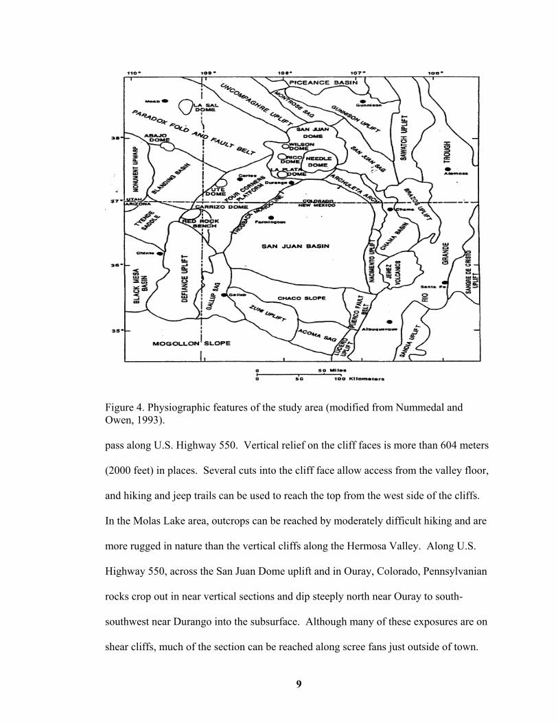
Figure 4. Physiographic features of the study area (modified from Nummedal and Owen, 1993). pass along U.S. Highway 550. Vertical relief on the cliff faces is more than 604 meters

(2000 feet) in places. Several cuts into the cliff face allow access from the valley floor,

and hiking and jeep trails can be used to reach the top from the west side of the cliffs.

In the Molas Lake area, outcrops can be reached by moderately difficult hiking and are

more rugged in nature than the vertical cliffs along the Hermosa Valley. Along U.S.

Highway 550, across the San Juan Dome uplift and in Ouray, Colorado, Pennsylvanian

rocks crop out in near vertical sections and dip steeply north near Ouray to south-

southwest near Durango into the subsurface. Although many of these exposures are on

shear cliffs, much of the section can be reached along scree fans just outside of town.

10

2.2 Stratigraphy of Study Area

The Lower-Middle Pennsylvanian Hermosa Group across the Paradox Basin and

surrounding areas is the focus of this study. Figure 5 delineates the internal and

Figure 5. Stratigraphic Column for study area, Four Corners region, western United States. structural relationships exposed in the study area respectively.

Basement geology in the study area is thought to have set the stage for overall

deposition in the Paleozoic strata of interest (Stevenson and Baars, 1984). Reactivation

of basement faults has long been considered a primary control on both structural

development and depositional architecture (Stevenson and Baars, 1984). The effects are

11

seen in each geologic system from the Precambrian to the Permian including the

stratigraphy of the Hermosa Group (Stevenson and Baars, 1984).

The present structural interpretation of the Paradox Basin is described as a

"complex pull-apart basin of large proportions" (Stevenson and Baars, 1984). The

Paradox Basin and the adjacent San Juan Basin were affected by the same geologic

processes, from Late Proterozoic time to the end of the Paleozoic. During

Pennsylvanian time, the Paradox Basin subsided rapidly as the Uncompahgre uplift rose

to the north and east. The area defined by the later development of the San Juan Basin

was relatively stable in comparison to the Paradox Basin and accumulated sediments at

a much slower rate during Pennsylvanian time (Dolson et al., 1992).

The stratigraphic successions in the Paradox Basin consist of a large evaporite

section within the Hermosa Group (Hite, 1960; Hite and Buckner, 1981; and Spoelhof,

1974). This includes the evaporitic Paradox Formation and its marine equivalents the

Barker Creek, Akah, Desert Creek, and Ismay members. The marine section is overlain

by the dominantly clastic section of the Honaker Trail Formation as defined by the

currently recognized stratigraphic definitions (Franczyk et al., 1993; Fig. 5).

A schematic diagram of the Paradox Basin (Fig. 6) shows that it is asymmetrical

from southwest to north-northeast. Structural development of the study area began in

Late Precambrian time approximately 1700 m.y. ago, during an interval of wrench

faulting involving the Olympic-Wichita (northwest trending) and Colorado (northeast

trending) lineament systems (Baars and Elingson, 1984, Stevenson and Baars, 1984).

12

Figure 6. Structural schematic diagram across the southern Paradox Basin western U.S.A. modified from Stevenson and Baars (1984), Hite and Buckner (1981), and Stroud (1994).

The structural fabric of the study area developed at the intersection of these lineaments.

During the development of the Ancestral Rockies, several Precambrian basement

structures were reactivated as strike slip faults (Stevenson and Baars, 1986). Figure 7

shows how this wrench system is thought to have developed. Influence of this

movement on sedimentation can be seen in the Pennsylvanian exposures in the Molas

Lake area where strata are uplifted and truncated in association with strike rotational

movement (Spoelhof, 1974).

The most dominant structural element affecting terrigenous clastic deposition in

the study area is the Uncompahgre Uplift. This highland was approximately in the

same position as the current Uncompahgre Mountains north and east of the Paradox

13

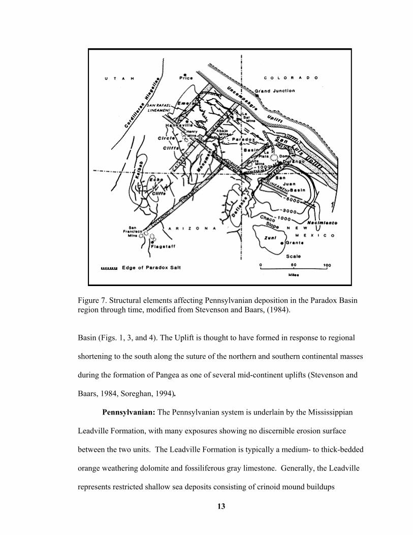
Figure 7. Structural elements affecting Pennsylvanian deposition in the Paradox Basin region through time, modified from Stevenson and Baars, (1984).

Basin (Figs. 1, 3, and 4). The Uplift is thought to have formed in response to regional

shortening to the south along the suture of the northern and southern continental masses

during the formation of Pangea as one of several mid-continent uplifts (Stevenson and

Baars, 1984, Soreghan, 1994).

Pennsylvanian: The Pennsylvanian system is underlain by the Mississippian

Leadville Formation, with many exposures showing no discernible erosion surface

between the two units. The Leadville Formation is typically a medium- to thick-bedded

orange weathering dolomite and fossiliferous gray limestone. Generally, the Leadville

represents restricted shallow sea deposits consisting of crinoid mound buildups

14

surrounded by lime muds (Spoelhof, 1974 and Franczyk et al., 1993). Following

shallow water marine deposition of the Ouray to Leadville sequence, the study area was

uplifted during the Antler orogenic event (Stevenson and Baars, 1984). Formation of the

Kaskaskia - Absaroka worldwide unconformity followed, separating the Mississippian

from the Pennsylvanian system in North America (Sloss, 1963). This sequence

boundary is marked in the study area by the occurrence of the Pennsylvanian (Atokan

age) Molas Formation, a paleosol formed on the karst surface of the underlying

Mississippian (Osagean age) Leadville dolomite. This surface is marked by a lacuna or

gap in the stratigraphic record of approximately 20 m.y. duration (Nummedal and

Owens, 1993). According to Wengerd and Matheny (1958) “The contact appears to be

transitional between the uppermost fine-grained red siltstone or shale bed of the

Leadville Formation, and beneath the first gray shale and limestone interval of the

Pinkerton Trail Formation”. This basal formation underlies the Pennsylvanian Hermosa

Group, resulting from dramatic changes in depositional patterns during the

Pennsylvanian, which is the focus of this study.

The Middle Pennsylvanian Hermosa Group (Desmoinesian age) is developed

stratigraphically above the Mississippian Leadville Formation and is marked at its base

by the Molas Formation, (Fig. 8;Wengerd and Strickland, 1958). The Hermosa Group

was first identified by Cross and Spencer (1900) in the Hermosa Cliffs near the town of

Hermosa, Colorado (Fig. 8). Baker et al. (1933) subdivided the Hermosa into members,

a lower and upper members separated by the Paradox member. These three units have

been raised to formational rank and are designated the Honaker Trail, Paradox, and

Pinkerton Trail formations (Fig. 5; Wengerd and Strickland, 1958).

15

The Paradox Formation was described by Wengerd and Strickland (1958) as

consisting of cyclic successions of halite and associated evaporite lithologies in the

Paradox Basin near Moab, Utah. This situation is not encountered at the designated type

section (Roth, 1934, Wengerd and Strickland, 1954; Wengerd and Matheny, 1958;

Wengerd, 1962; and Wengerd and Szabo, 1968). There was general recognition of the

lateral and vertical relationships of the Paradox Formation to the Honaker Trail

Formation; however, the Paradox Formation is not found at the type section location in

the Animas Valley. This study and other more recent evaluations (Spoelhof, 1974;

Franczyk et al., 1993) consider that the stratigraphy at the type section, while

lithostratigraphically equivalent to the Honaker Trail Formation, is

chronostratigraphically equivalent to the Paradox formation in the central part of the

basin. This issue is discussed in Chapter 5.

In the continuing process of refining the stratigraphic relationships of the

Pennsylvanian system in the Paradox Basin, Wengerd and Strickland (1954), Wengerd

and Matheny (1958), and Wengerd (1962), proposed that the Hermosa Formation be

raised to group status. The suggestion was that the group be comprised of three

members: a lower member designated as the Pinkerton Trail Formation, followed by the

Paradox Formation and the Honaker Trail Formation at the top. These descriptions are

primarily lithostratigraphic divisions that may be time transgressive. Definition of a

16

Figure 8. Location map of key stratigraphic outcrop sections with surface geology in the Animas Valley area. Surface exposures of Pennsylvanian age sediments are gray in color, modified from USGS Durango East Quad map.

more definitive genetic relationship between these formations is an outcome of this

study and is discussed below.

The Pinkerton Trail Formation is the basal unit of the Hermosa Group. It is

composed of a sequence of marine carbonate rocks with black and dark-gray shale with

little detrital material. This marine section reflects the reintroduction of marine

conditions following terminal Mississippian regression. It overlies the Molas paleosol,

is time transgressive from Early to Middle Pennsylvanian (Atokan-Desmoinesian), and

ranges in thickness from 0-60 meters (0-200 feet) (Wengerd and Matheny, 1958; Dr.

Donald Rasmussen personal communication, 1999). Whereas the Molas Formation is

easily recognized in outcrop, the unit is difficult to distinguish in the subsurface from

the Pinkerton Formation.

17

The Pinkerton Trail Formation generally shows a gradual shallowing up-section

with wackestone and packstone textures dominating. Corals and algae present in the

rocks are the diagnostic time and environmental features used to define these events

(Spoelhof, 1974). At Molas Lake, the Pinkerton Trail is divided into three units: a

poorly stratified marine siltstone at the base; a middle unit of thicker open marine

carbonate rocks; and an upper unit consisting of uniformly thin beds that display some

dolomitization that is indicative of shallow inter-tidal conditions (Spoelhof, 1974, p.40).

The Pinkerton Trail is extensive over the study area (Wengerd and Strickland, 1954).

Outcrops along the Animas valley on the eastern flank of Hermosa Mountain are late

Atokan to Early Desmoinesian in age based on fusulinid foraminifera, Fusulina,

Fusulinella and Wedekindellina, (this paper, see Appendix A). The Pinkerton Trail can

range in thickness from 11 meters (36 feet) in the southwest to greater then 84 meters

(275 feet) in the San Juan Mountains. Spoelhof (1974) identified biota consisting of

normal open marine assemblages including: bryozoans, brachiopods, solitary corals,

Chaetetes, and phylloid algae of Ivanovia and Komia. The lack of coarse clastic

sedimentary rock anywhere in the formation suggests that the early stage of formation

of the Uncompahgre Uplift had little impact on sedimentation and that shallow marine

conditions persisted across the region (Wengerd and Strickland, 1954).

The Paradox Formation is the middle member of the Hermosa Group and was

first identified in the Paradox Valley in west central Colorado by Baker et al. (1933).

The Paradox Formation, which is primarily observed in the middle of the Paradox

Basin, is dominated by evaporites. The evaporites are interbedded with open marine

carbonate rocks and shoaling-up carbonate buildups to the west, and terrigenous clastic

rocks to the north-northeast (Fig. 9). The evaporites alternate with black marine shales

18

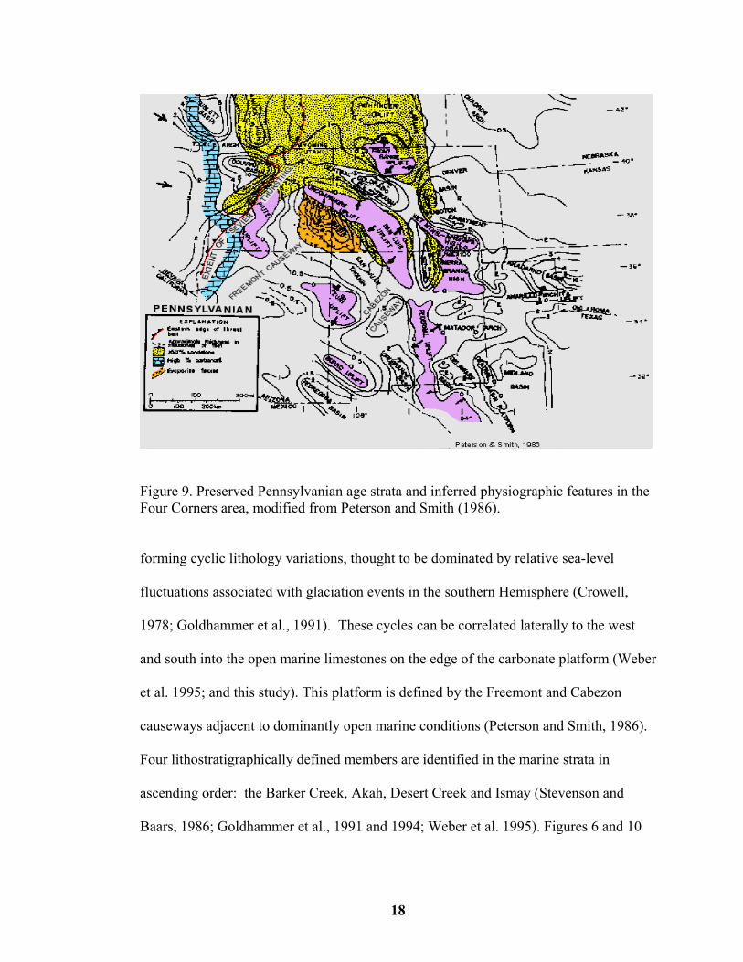
Figure 9. Preserved Pennsylvanian age strata and inferred physiographic features in the Four Corners area, modified from Peterson and Smith (1986).

forming cyclic lithology variations, thought to be dominated by relative sea-level

fluctuations associated with glaciation events in the southern Hemisphere (Crowell,

1978; Goldhammer et al., 1991). These cycles can be correlated laterally to the west

and south into the open marine limestones on the edge of the carbonate platform (Weber

et al. 1995; and this study). This platform is defined by the Freemont and Cabezon

causeways adjacent to dominantly open marine conditions (Peterson and Smith, 1986).

Four lithostratigraphically defined members are identified in the marine strata in

ascending order: the Barker Creek, Akah, Desert Creek and Ismay (Stevenson and

Baars, 1986; Goldhammer et al., 1991 and 1994; Weber et al. 1995). Figures 6 and 10

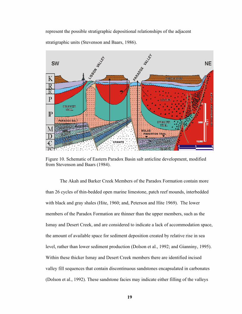
19

represent the possible stratigraphic depositional relationships of the adjacent

stratigraphic units (Stevenson and Baars, 1986).

Figure 10. Schematic of Eastern Paradox Basin salt anticline development, modified from Stevenson and Baars (1984).

The Akah and Barker Creek Members of the Paradox Formation contain more

than 26 cycles of thin-bedded open marine limestone, patch reef mounds, interbedded

with black and gray shales (Hite, 1960; and, Peterson and Hite 1969). The lower

members of the Paradox Formation are thinner than the upper members, such as the

Ismay and Desert Creek, and are considered to indicate a lack of accommodation space,

the amount of available space for sediment deposition created by relative rise in sea

level, rather than lower sediment production (Dolson et al., 1992; and Gianniny, 1995).

Within these thicker Ismay and Desert Creek members there are identified incised

valley fill sequences that contain discontinuous sandstones encapsulated in carbonates

(Dolson et al., 1992). These sandstone facies may indicate either filling of the valleys

20

during low relative sea level or rapid filling during sea level rise into long-term relative

sea level highstand as surmised by this author. Thus, the long held believe that these

distal valley fill sandstones are only developed during relative sea level lowstands is

suspect and will be investigated during the course of this study.

The Desert Creek member overlies the Akah member of the Paradox Formation

and is divided into upper and lower units that have distinctive highstand and lowstand

components. The majority of the hydrocarbon production in the study area is produced

from the lower Desert Creek at the Aneth Field complex, a highstand algal mound

facies (Fig. 3, Weber et al., 1995). The Papoose Canyon Field also produces from the

lower Desert Creek but is associated with the lowstand carbonate shoreline facies

(Dolson et al., 1992). The upper and lower Desert Creek have similar lithologic

characteristics. However, at the Aneth Field area, no major reefal builders occur in the

upper unit (Figs. 5 and 6) (Dolson et al., 1992).

The Desert Creek is onlapped from north to south by the Ismay Member the

uppermost unit in the Paradox Formation (Dolson et al. 1992). The top of the Ismay is

marked by evaporites that transition into a shallowing upward marine succession

generally consisting of shallow open marine muds and mound buildups with associated

evaporites. The Ismay member is also divided into upper and lower units. Facies

within the Ismay section are similar to the underlying Desert Creek member (Dolson et

al., 1992). The upper Ismay coincides with a decrease in overall evaporite production

in the basin and is overlain by the prograding Honaker Trail Formation that defines the

top of the Hermosa Group.

The Honaker Trail Formation consists of several lithofacies: fan delta complexes

composed of coarse-grained arkosic sandstones in more proximal locations and

21

becoming more medium grained in marine fan-delta and valley fill facies; shales from

both open marine transgressions and terrigenous delta development; and open to

restricted marine limestones up to 914 meters (3000 feet) thick. These limestones occur

above the uppermost evaporite bed in Paradox Formation. Many of the Pennsylvanian

age outcrops in the San Juan Mountains are composed of these alternating marine

carbonates and terrigenous clastic alluvial fan-fan delta successions (Spoelhof, 1974,

Stevenson and Baars, 1984).

In the parts of the basin floored by evaporites, loading of the Honaker Trail is

thought to have caused early diapirism, that continued into Jurassic time (Fig. 10). The

Paradox Formation is generally missing in the outcrop sections of the San Juan Dome

area. The absence of the Paradox Formation, as well as its possible time equivalence to

parts of the Honaker Trail Formation, had previously been an unresolved. Regional

correlation work in this study demonstrates that parts of the Paradox are physically

continuous with parts of the Honaker Trail (discussed in Chapter 4 and 5).

Between Coal Bank Pass and Silverton, the Pennsylvanian section consists of

the Pinkerton Trail Formation that grades upward into Honaker Trail Formation. The

Honaker Trail Formation in this area consists of three units designated as upper-middle-

lower undifferentiated Honaker Trail (Spoelhof, 1974). The upper and lower Honaker

Trail members are dominated by terrigenous clastic sedimentary rocks and the middle

Honaker trail member is dominantly marine carbonate rock. The middle unit has been

correlated along U.S. Highway 550 near the original type section at Hermosa, Colorado

(Franczyk et al., 1993). Each of the cycles identified in the Honaker Trail represents

marine to deltaic sedimentation that show gradual shoaling up section. Of particular

interest is a gypsum unit described by Franczyk et al. (1993) in the type section.

22

Franczyk noted that this unit might correlate to cycle 6 the most extensive evaporite unit

identified in the Paradox Basin by Hite (1960).

The abrupt deepening of the Paradox Basin during Pennsylvanian time is

recorded in open marine limestones. These units are found at the base of many of the

cycles in the more proximal terrigenous clastic cycles. These facies are thought to

represent the effects of moderate sea-level changes in a relatively shallow shelf platform

environment that was in close proximity to clastic depocenters off the Uncompahgre

uplift (Spoelhof, 1974; Weber et al, 1985). The ability to correlate these cyclic beds

across the platform from terrigenous clastic dominated outcrops to subsurface carbonate

dominated units is required in order to achieve the goals of this study.

Waning of Pennsylvanian time deposition in the study area is indicated by the

change from dominantly marine sedimentary rocks to the continental red-beds of the

Permian time. Permian deposition begins as subsidence rates in the Four Corners region

decreased and the land becomes emergent. Permian continental sedimentary rocks

began to dominate the study area as evidenced by the red arkosic and conglomeritic

sandstones of the Cutler Formation that were derived from the Uncompahgre Uplift

(Fig. 11) (Spoelhof, 1974; Campbell, 1979). Dark-red shales representing transition

from marine to continental conditions are found within this increasingly continentally

dominated section (Campbell, 1979). The Cutler Formation is defined to overly the

uppermost marine limestone of the Honaker Trail Formation, which is locally named as

the "Rico Formation" (Spoelhof, 1974).

23

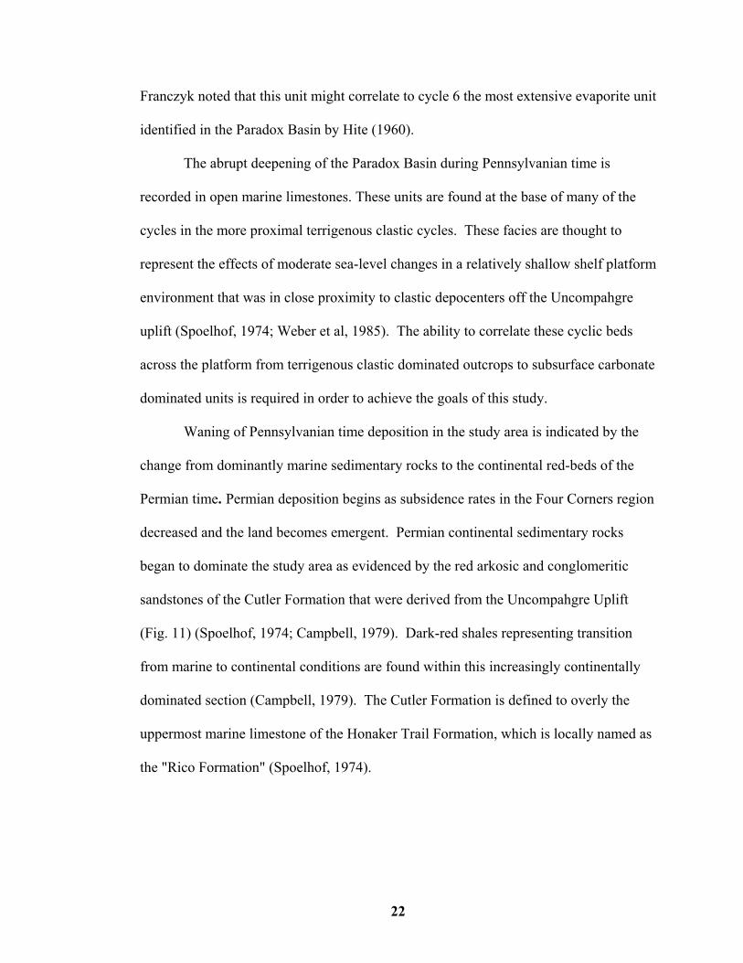
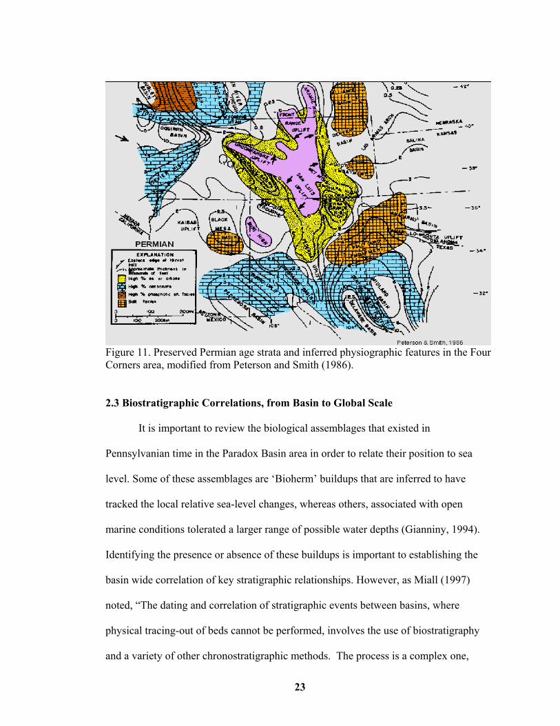
Figure 11. Preserved Permian age strata and inferred physiographic features in the Four Corners area, modified from Peterson and Smith (1986).

2.3 Biostratigraphic Correlations, from Basin to Global Scale

It is important to review the biological assemblages that existed in

Pennsylvanian time in the Paradox Basin area in order to relate their position to sea

level. Some of these assemblages are ‘Bioherm’ buildups that are inferred to have

tracked the local relative sea-level changes, whereas others, associated with open

marine conditions tolerated a larger range of possible water depths (Gianniny, 1994).

Identifying the presence or absence of these buildups is important to establishing the

basin wide correlation of key stratigraphic relationships. However, as Miall (1997)

noted, “The dating and correlation of stratigraphic events between basins, where

physical tracing-out of beds cannot be performed, involves the use of biostratigraphy

and a variety of other chronostratigraphic methods. The process is a complex one,

24

fraught with many possible sources of errors”. Thus, understanding what the source

and ranges of error uncertainty in correlating chronostratigraphically inferred

relationships are important to determining the possible stratigraphic relationships

identified in the Paradox Basin.

Fusulinid faunas from the Eastern and mid-continent of the United States have

long supplied the primary faunal divisions utilized to delineate age relationships for the

Pennsylvanian System in North America (Wahlman, 1999). More recently, conodont

faunas are supplementing the fusulinid data in defining the biostratigraphic zones in the

Pennsylvanian strata of the Paradox Basin, because conodont analysis allows more

precise correlation to the mid-continent successions (Nail et al., 1996). In this study,

biostratigraphic delineation was a secondary concern and was primarily utilized to

determine the stratigraphic position of the newly measured section in the Animas

Valley. Ultimately, however, an inference of the chronostratigraphic significance of the

stratigraphic relationships of the Pennsylvanian age rocks in the Paradox Basin is

necessary if global versus local controls on sedimentation are to be determined.

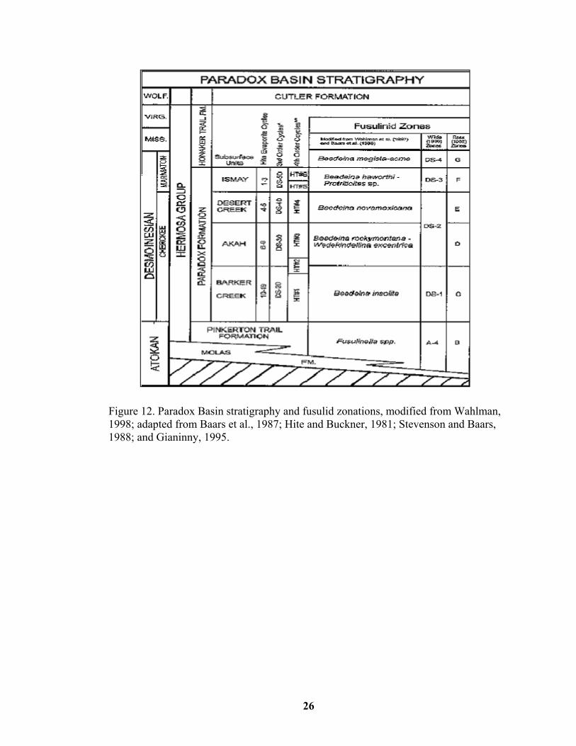
Wahlman (1999) noted that the Desmoinesian Stage of the Pennsylvanian

System has been generally subdivided into four fusulinid subzones for regional

correlation, Table 1.

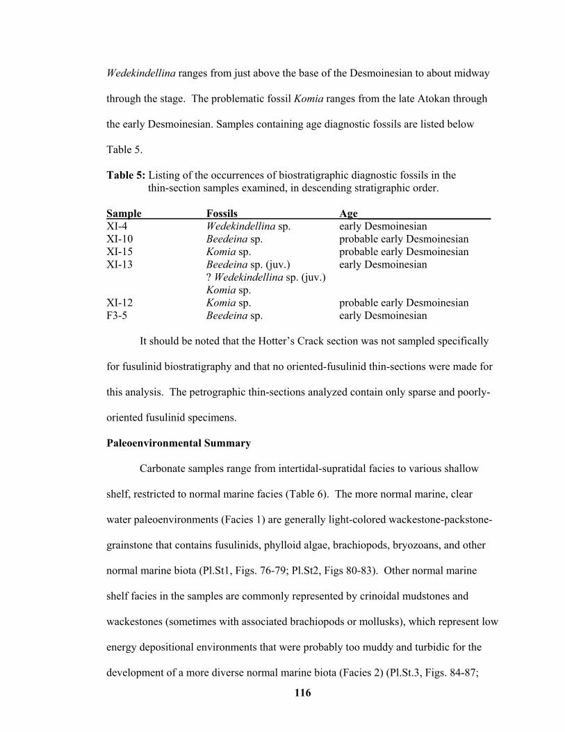
“Of the thirty-two samples examined from the Hotter’s Crack Section for this study, six samples contained age-diagnostic fossils. All six of these samples are early Desmoinesian in age, based on the occurrences of the fusulinids Beedeina sp. and Wedekindellina sp., and the problematic fossil Komia a calcareous red algae (Rhodophyta). The fusulinid genus Beedeina ranges from the base to the top of the Desmoinesian. All of the specimens of Beedeina sp. identified here appear to be relatively primitive forms of the genus. The fusulinid genus Wedekindellina ranges from just above the base of the Desmoinesian to about midway through the stage. The problematic fossil Komia ranges from the late Atokan through the early Desmoinesian” (Wahlman, 1999, Appendix A and Fig. 12).

25

Table 1: Standard Desmoinesian fusulinid subzones and their corresponding lithostratigraphic units in the Mid-Continent USA region (Wahlman, 1999).

_______________________________________________ Mid-continent Units Fusulinid Subzones

Upper Marmaton Group Beedeina eximia-B.acme

Lower Marmaton Group Beedina girtyi-B. haworthi

Upper Cherokee Group Beedina novamexicana-

Wedekindellina euthysepta

Lower Cherokee Group Beedeina insolita-B. leei.

These inferences are consistent with analysis completed by Spoelhof (1974) to the north

of the Hotter’s Crack section and Franczyk et al. (1993) at the Hermosa type section to

the south. Spoelhof (1974) identified fusulinid species Wedekindellina, Fusulina, F.

pristina, Eoschubertella and Fusulinella. Therefore, as Wahlman has previously noted,

the sections in the Animas Valley generally resides in the Desmoinesian stage of the

Pennsylvanian but the age designation of the internal cycles can not be refined to 4th or

5th order levels making it difficult to correlate specific chronostratigraphic intervals

regionally.

26

Figure 12. Paradox Basin stratigraphy and fusulid zonations, modified from Wahlman, 1998; adapted from Baars et al., 1987; Hite and Buckner, 1981; Stevenson and Baars, 1988; and Gianinny, 1995.

27

CHAPTER 3. LITHOLOGIC CALIBRATION OF ROCKTYPES TO IN-SITU WELLBORE MEASUREMENTS

3.1 Chapter Overview

From Hutton's 1785 "principles of uniformitarianism", Davis (1898) gives a

framework for associating "observed geologic effects with competent causes"

(Nummedal, 1993). Observed geologic effects are manifested in the development of

genetically related successions of depositional facies that reflect specific depositional

forces. In this study, the effects of eustasy and tectonism (causes) on the stratigraphic

patterns developed in the Hermosa Group of the Paradox Basin have been related to

outcrop and subsurface data sets. These data sets encompass juxtaposed depositional

facies and cannot be looked at separately if the objectives of this study are to be met.

These successions consist of carbonate, evaporite, and siliciclastic depositional systems.

Emphasis is on relating rock-data to wireline measurements and inferring stacking

pattern hierarchies, lateral correlation accuracy, and process dependencies on the

stratigraphic succession development in the Hermosa Group.

A fundamental concept used in predicting facies relationships is often predicted

using the concept of stratal "stacking patterns" (Posamentier et al., 1988). To predict

the lateral facies distribution, a determination is needed of what genetically related

internal depositional facies constitute a specific succession within a stacking pattern.

Succession implies a linkage between what came before with what comes after. In the

study of stratigraphy, ‘succession’ is defined as, “a number of rock units or a mass of

strata that succeed one another in chronologic order; e.g. an inclusive stratigraphic

sequence involving any number of stages, series, systems, or parts thereof, seen in an

exposed section” (Bates and Jackson, 1987). Based on this concept, geologists have

observed that many depositional successions in the rock record repeat themselves in

28

whole or part within a stratigraphic framework. This observation of repeatability, i.e.

cyclicity, can be recognized in the stratigraphic record is fundamental to the study of

stratigraphy.

Once specific facies successions are defined and repeatable units recognized, a

determination of the types and numbers of depositional sequences can be inferred.

These defined depositional sequences can then be used to evaluate the lateral and

temporal extent of the depositional elements that produced them. This section presents

the methods and results of defining these facies succession relationships in the study.

3.2. Measured Section at Hotter’s Crack

To supplement previous work done on stratigraphic analysis in the study area, a

new section of the Pennsylvanian Hermosa Group was measured along the Hermosa

Cliffs 21 miles north of Durango, Colorado on the west side of the Animas River Valley

(Fig. 13). The section has its base at the top of the Molas Formation near Purgatory Ski

Resort to its top at Hotter’s Crack 1.5 miles to the south along Highway 550 (Fig.14).

This measured section lies between the type section at Hermosa Mountain and the

Molas Lake area of the San Juan Dome complex. The section consists of basin-margin

marine/evaporite facies co-mingled with terrigenous clastic fan-delta successions.

3.2.1 Outcrop Measurement Techniques

The Purgatory to Hotter’s Crack measured section is composed of nine segments (A-I)

located at approximately (latitude, 37.61115 N. and longitude, –107.84560 W.), (Figure

14, Electra Lake, 7.5 minute quadrangle). The lower segments of the measured

29

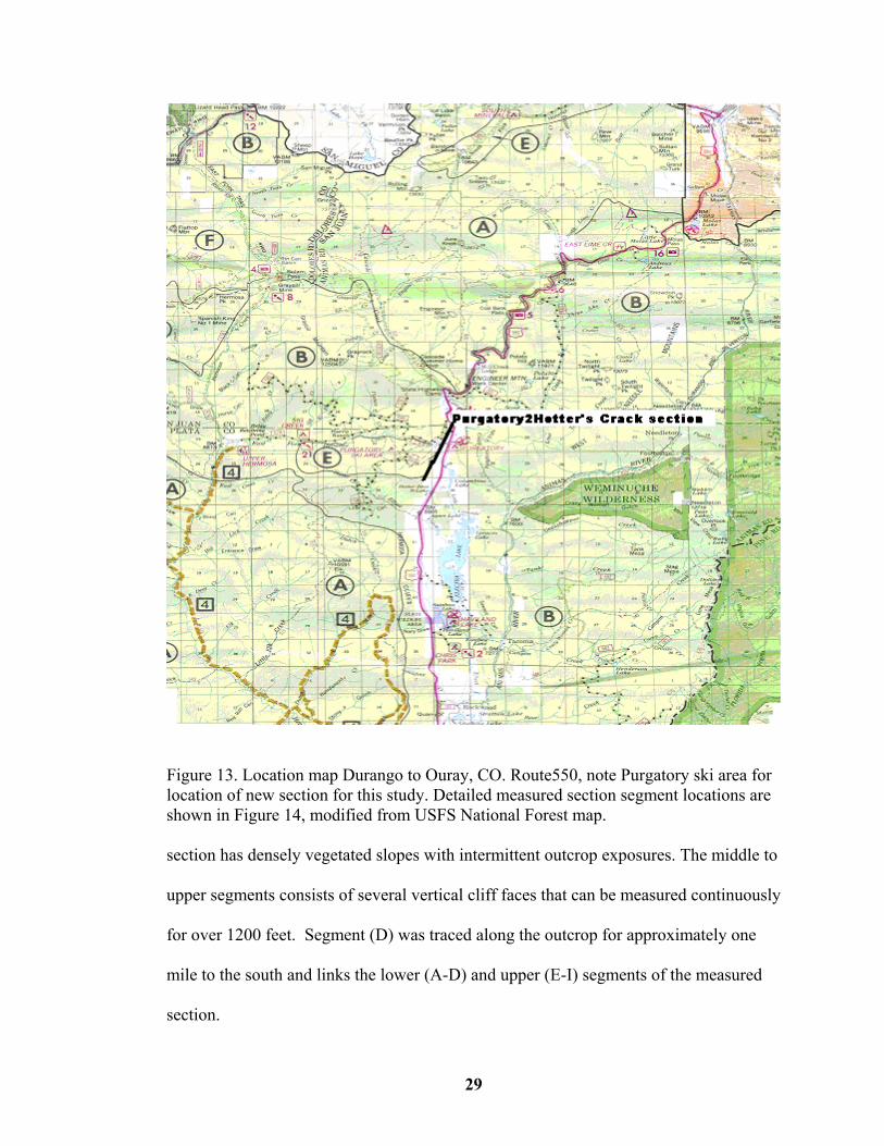
Figure 13. Location map Durango to Ouray, CO. Route550, note Purgatory ski area for location of new section for this study. Detailed measured section segment locations are shown in Figure 14, modified from USFS National Forest map. section has densely vegetated slopes with intermittent outcrop exposures. The middle to

upper segments consists of several vertical cliff faces that can be measured continuously

for over 1200 feet. Segment (D) was traced along the outcrop for approximately one

mile to the south and links the lower (A-D) and upper (E-I) segments of the measured

section.

30

Outcrop Sections at Purgatory to Hotter’s Crack.

Base of section start at segm ent A

Top of section segm ent I

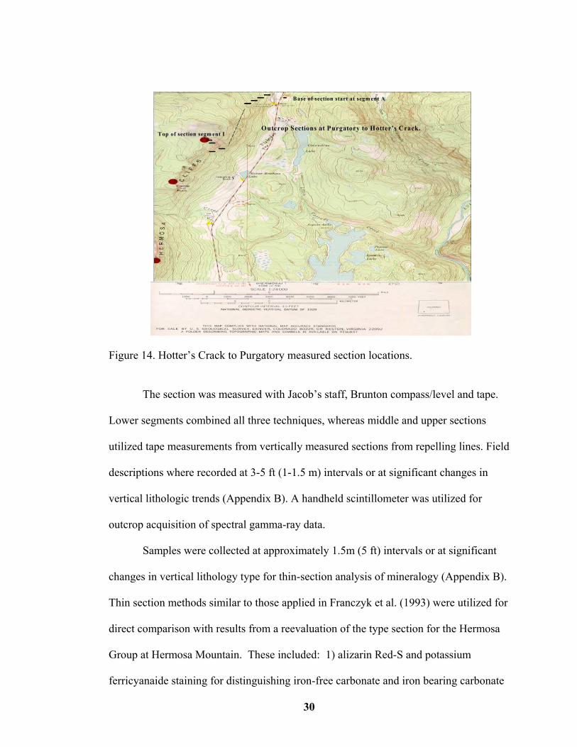
Figure 14. Hotter’s Crack to Purgatory measured section locations.

The section was measured with Jacob’s staff, Brunton compass/level and tape.

Lower segments combined all three techniques, whereas middle and upper sections

utilized tape measurements from vertically measured sections from repelling lines. Field

descriptions where recorded at 3-5 ft (1-1.5 m) intervals or at significant changes in

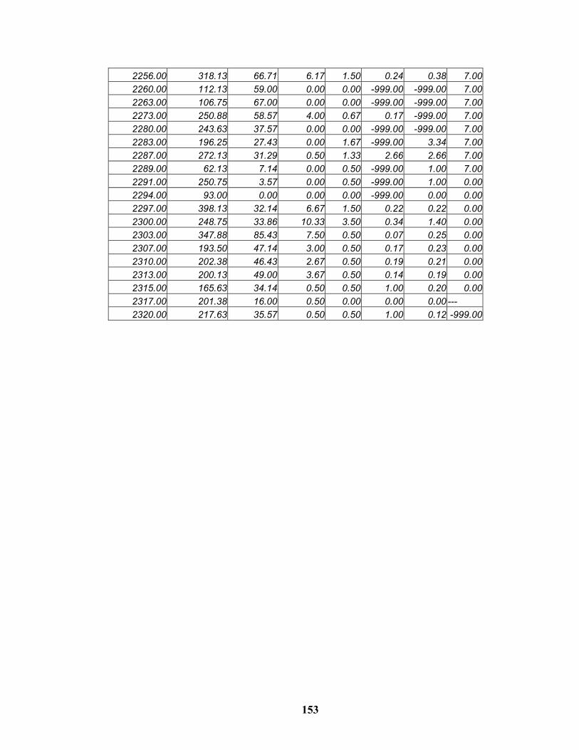
vertical lithologic trends (Appendix B). A handheld scintillometer was utilized for

outcrop acquisition of spectral gamma-ray data.

Samples were collected at approximately 1.5m (5 ft) intervals or at significant

changes in vertical lithology type for thin-section analysis of mineralogy (Appendix B).

Thin section methods similar to those applied in Franczyk et al. (1993) were utilized for

direct comparison with results from a reevaluation of the type section for the Hermosa

Group at Hermosa Mountain. These included: 1) alizarin Red-S and potassium

ferricyanaide staining for distinguishing iron-free carbonate and iron bearing carbonate

31

minerals; and 2) sodium cobaltinitrite stain for identifying potassium-feldspar grains.

These staining methods improve identification of calcite, dolomite, ferroan calcite, and

ferroan dolomite minerals within the carbonate assemblages, and feldspars with the

quartz sandstone assemblages. Mineral abundance, grain sorting, roundness, and size

distributions where estimated visually. In addition, the paleontological content of the

carbonate samples were evaluated with specific emphasis on fusulinid genera

identifications (Dr. G. Wahlman, Amoco Production Company, Appendix A).

Figure 38 is a small-scale profile of the upper segment of the Purgatory to

Hotter’s Crack measured section showing the major lithologic units. The middle to

upper members of the measured section at Hotter’s Crack contains alternating

successions of open marine limestone (light gray), terrigenous clastics (white to light

brown) and intervening shales (darker gray) can be seen (Fig. 15, 4, and 5).

This section shows nicely the sharp contacts between the open marine limestone units

and the fan-delta clastics. This contrast can best be seen in the outcrop sections (G, H,

and I) from the Hotter’s Crack location (Figures 16 and 17). Figure 17 show the contrast

of the outcrop relationships to a subsurface well 20 miles to the southwest. In each case,

the fan-delta clastics have in general sharp contacts with the limestone units with little

to no transitional fine mud intervals. There are several instances where the contact

between the limestones and the fan-delta clastics is very sharp at both the top and the

base of the clastics. This suggests that that the clastic sediments were deposited during

both sea level lowstand, where the clastics downlap the carbonate facies, as well as, sea

level highstand, where they are deposited quickly into the open marine

32

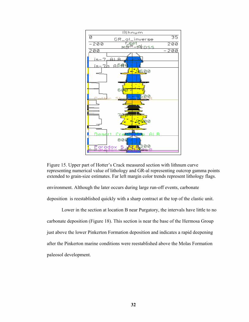
Figure 15. Upper part of Hotter’s Crack measured section with lithnum curve representing numerical value of lithology and GR-al representing outcrop gamma points extended to grain-size estimates. Far left margin color trends represent lithology flags. environment. Although the later occurs during large run-off events, carbonate

deposition is reestablished quickly with a sharp contract at the top of the clastic unit.

Lower in the section at location B near Purgatory, the intervals have little to no

carbonate deposition (Figure 18). This section is near the base of the Hermosa Group

just above the lower Pinkerton Formation deposition and indicates a rapid deepening

after the Pinkerton marine conditions were reestablished above the Molas Formation

paleosol development.

33

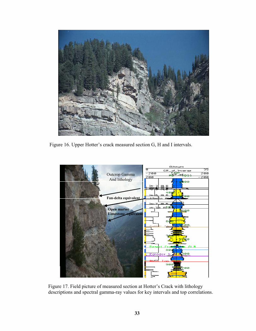
Figure 16. Upper Hotter’s crack measured section G, H and I intervals.

Put my measured Here! Or as separateSlide next to this.

Outcrop GammaAnd lithology

Fan-delta equivalent

Open marine Limestone equivalent

Figure 17. Field picture of measured section at Hotter’s Crack with lithology descriptions and spectral gamma-ray values for key intervals and top correlations.

34

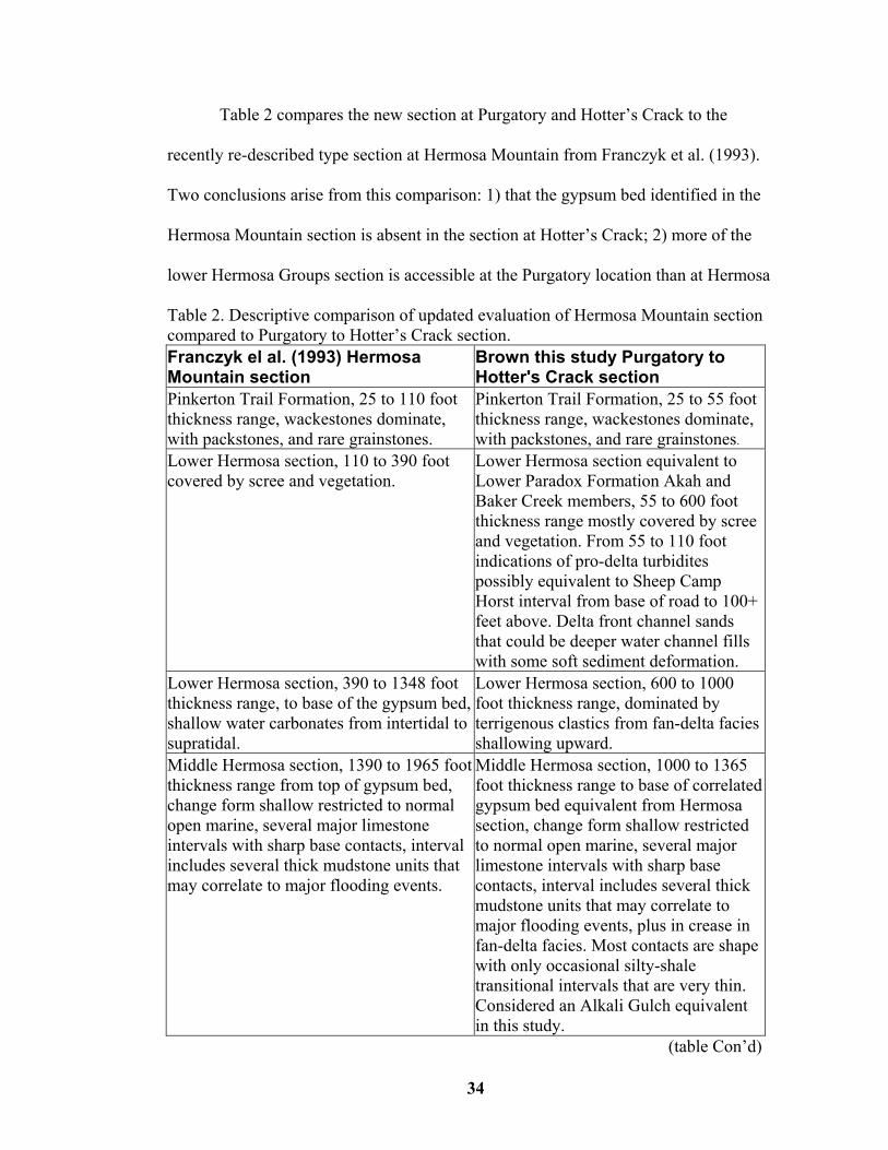
Table 2 compares the new section at Purgatory and Hotter’s Crack to the

recently re-described type section at Hermosa Mountain from Franczyk et al. (1993).

Two conclusions arise from this comparison: 1) that the gypsum bed identified in the

Hermosa Mountain section is absent in the section at Hotter’s Crack; 2) more of the

lower Hermosa Groups section is accessible at the Purgatory location than at Hermosa

Table 2. Descriptive comparison of updated evaluation of Hermosa Mountain section compared to Purgatory to Hotter’s Crack section. Franczyk el al. (1993) Hermosa Mountain section

Brown this study Purgatory to Hotter's Crack section

Pinkerton Trail Formation, 25 to 110 foot thickness range, wackestones dominate, with packstones, and rare grainstones.

Pinkerton Trail Formation, 25 to 55 foot thickness range, wackestones dominate, with packstones, and rare grainstones.

Lower Hermosa section, 110 to 390 foot covered by scree and vegetation.

Lower Hermosa section equivalent to Lower Paradox Formation Akah and Baker Creek members, 55 to 600 foot thickness range mostly covered by scree and vegetation. From 55 to 110 foot indications of pro-delta turbidites possibly equivalent to Sheep Camp Horst interval from base of road to 100+ feet above. Delta front channel sands that could be deeper water channel fills with some soft sediment deformation.

Lower Hermosa section, 390 to 1348 foot thickness range, to base of the gypsum bed, shallow water carbonates from intertidal to supratidal.

Lower Hermosa section, 600 to 1000 foot thickness range, dominated by terrigenous clastics from fan-delta facies shallowing upward.

Middle Hermosa section, 1390 to 1965 foot thickness range from top of gypsum bed, change form shallow restricted to normal open marine, several major limestone intervals with sharp base contacts, interval includes several thick mudstone units that may correlate to major flooding events.

Middle Hermosa section, 1000 to 1365 foot thickness range to base of correlated gypsum bed equivalent from Hermosa section, change form shallow restricted to normal open marine, several major limestone intervals with sharp base contacts, interval includes several thick mudstone units that may correlate to major flooding events, plus in crease in fan-delta facies. Most contacts are shape with only occasional silty-shale transitional intervals that are very thin. Considered an Alkali Gulch equivalent in this study.

(table Con’d)

35

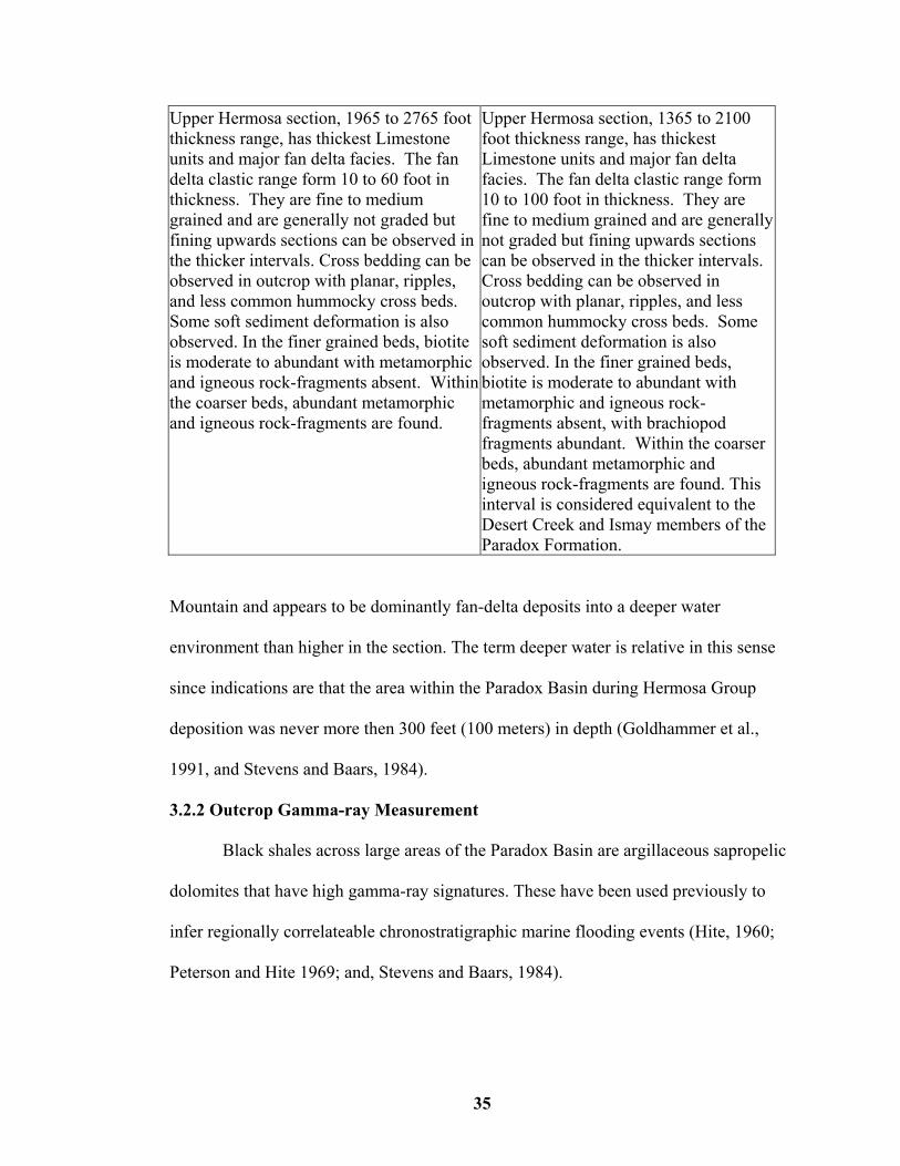
Upper Hermosa section, 1965 to 2765 foot thickness range, has thickest Limestone units and major fan delta facies. The fan delta clastic range form 10 to 60 foot in thickness. They are fine to medium grained and are generally not graded but fining upwards sections can be observed in the thicker intervals. Cross bedding can be observed in outcrop with planar, ripples, and less common hummocky cross beds. Some soft sediment deformation is also observed. In the finer grained beds, biotite is moderate to abundant with metamorphic and igneous rock-fragments absent. Within the coarser beds, abundant metamorphic and igneous rock-fragments are found.

Upper Hermosa section, 1365 to 2100 foot thickness range, has thickest Limestone units and major fan delta facies. The fan delta clastic range form 10 to 100 foot in thickness. They are fine to medium grained and are generally not graded but fining upwards sections can be observed in the thicker intervals. Cross bedding can be observed in outcrop with planar, ripples, and less common hummocky cross beds. Some soft sediment deformation is also observed. In the finer grained beds, biotite is moderate to abundant with metamorphic and igneous rock-fragments absent, with brachiopod fragments abundant. Within the coarser beds, abundant metamorphic and igneous rock-fragments are found. This interval is considered equivalent to the Desert Creek and Ismay members of the Paradox Formation.

Mountain and appears to be dominantly fan-delta deposits into a deeper water

environment than higher in the section. The term deeper water is relative in this sense

since indications are that the area within the Paradox Basin during Hermosa Group

deposition was never more then 300 feet (100 meters) in depth (Goldhammer et al.,

1991, and Stevens and Baars, 1984).

3.2.2 Outcrop Gamma-ray Measurement

Black shales across large areas of the Paradox Basin are argillaceous sapropelic

dolomites that have high gamma-ray signatures. These have been used previously to

infer regionally correlateable chronostratigraphic marine flooding events (Hite, 1960;

Peterson and Hite 1969; and, Stevens and Baars, 1984).

36

Passive nuclear logs called gamma-ray logs measure the natural gamma ray

intensity from rocks observed in boreholes and outcrops. There are two types of

passive gamma-ray (GR) logs, those that record the total gamma ray count and those

D e lta F r o n t T u r b id iteF in in g u p fa c ie s C -D

D e lta F r o n t T u r b id iteF a c ie s D -E

B a se o f H e r m o sa G r o u p S e c t io n B a t P u r g a to r y

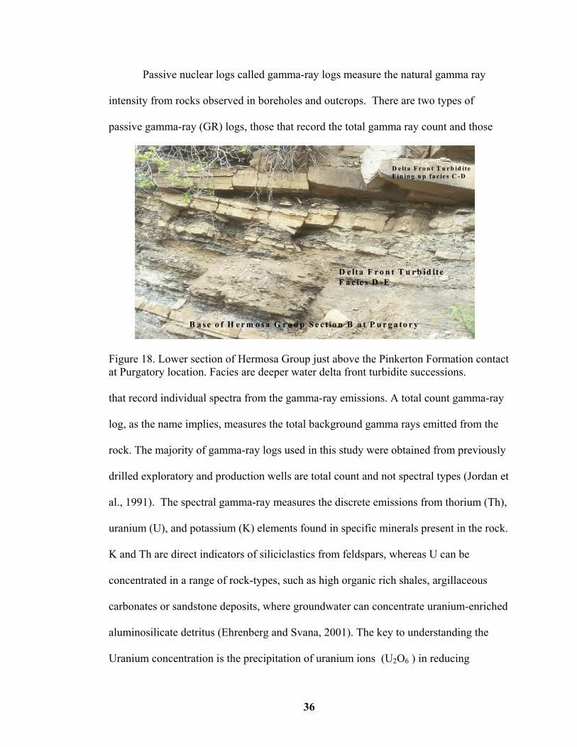
Figure 18. Lower section of Hermosa Group just above the Pinkerton Formation contact at Purgatory location. Facies are deeper water delta front turbidite successions. that record individual spectra from the gamma-ray emissions. A total count gamma-ray

log, as the name implies, measures the total background gamma rays emitted from the

rock. The majority of gamma-ray logs used in this study were obtained from previously

drilled exploratory and production wells are total count and not spectral types (Jordan et

al., 1991). The spectral gamma-ray measures the discrete emissions from thorium (Th),

uranium (U), and potassium (K) elements found in specific minerals present in the rock.

K and Th are direct indicators of siliciclastics from feldspars, whereas U can be

concentrated in a range of rock-types, such as high organic rich shales, argillaceous

carbonates or sandstone deposits, where groundwater can concentrate uranium-enriched

aluminosilicate detritus (Ehrenberg and Svana, 2001). The key to understanding the

Uranium concentration is the precipitation of uranium ions (U2O6 ) in reducing

37

environments. The intensity of K40 is a measure of the amount of clay minerals

produced from feldspar dissolution.

Outcrop data acquired for this study at the Hotter’s Crack section, was

integrated with previous work of Spoelhof (1974) in the Molas Lake area of the San

Juan Dome region, and of Franczyk et al. (1992 and 1993) from outcrop studies of

Pennsylvanian rocks near Hermosa, and Ouray, Colorado. All outcrop data from this

and previously completed studies from the area were transformed into a digital format

for study. Pseudo gamma-ray logs were calibrated by using outcrop gamma-ray data

obtained in this study (Fig. 19). These data are used to calibrate the detailed lithologic

definitions from the outcrop sections to the subsurface wireline data. Results from the

upper part of the measured section are presented in Figures 20 and 21. The data

displayed includes: lithology descriptions for the measured section with Spectral

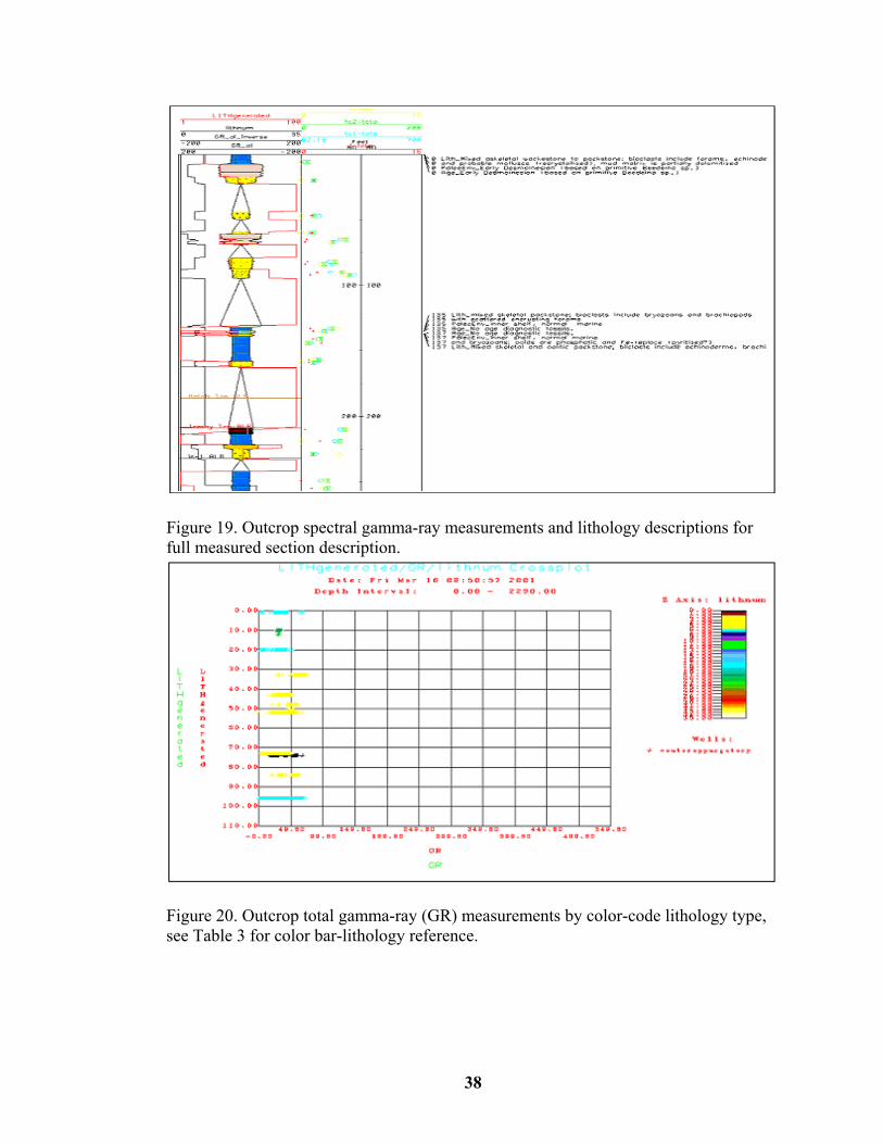
gamma-ray counts of Total GR (API), Th ppm, U ppm, and K ppm. A total of 96-

outcrop measurements were acquired in the Hotter’s Crack section. The complete

section measurements are found in Appendix (C). In the outcrop section, no high

gamma ray intervals were found (Fig. 21). Crossplots of the spectral components did

not indicate any definitive relationships. If lithology controlled the distribution of the

spectral minerals specific ratio plots would show significant variation from a one-to-one

relationship (Jordan et al., 1991a and 1991b; Jordan, 1993). Neither the Th/K nor Th/U

ratios could be used to discriminate the many different lithology types with ratios

generally less than 1 (Figs. 19, 20, 21 and 22).

38

Figure 19. Outcrop spectral gamma-ray measurements and lithology descriptions for full measured section description.

Figure 20. Outcrop total gamma-ray (GR) measurements by color-code lithology type, see Table 3 for color bar-lithology reference.

39

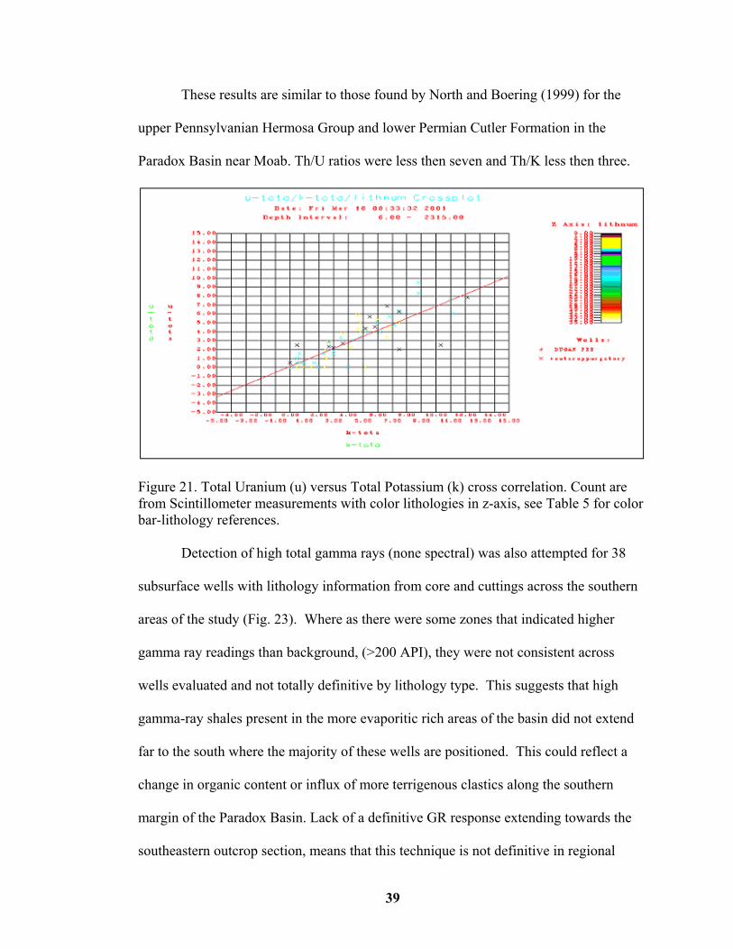
These results are similar to those found by North and Boering (1999) for the

upper Pennsylvanian Hermosa Group and lower Permian Cutler Formation in the

Paradox Basin near Moab. Th/U ratios were less then seven and Th/K less then three.

Figure 21. Total Uranium (u) versus Total Potassium (k) cross correlation. Count are from Scintillometer measurements with color lithologies in z-axis, see Table 5 for color bar-lithology references.

Detection of high total gamma rays (none spectral) was also attempted for 38

subsurface wells with lithology information from core and cuttings across the southern

areas of the study (Fig. 23). Where as there were some zones that indicated higher

gamma ray readings than background, (>200 API), they were not consistent across

wells evaluated and not totally definitive by lithology type. This suggests that high

gamma-ray shales present in the more evaporitic rich areas of the basin did not extend

far to the south where the majority of these wells are positioned. This could reflect a

change in organic content or influx of more terrigenous clastics along the southern

margin of the Paradox Basin. Lack of a definitive GR response extending towards the

southeastern outcrop section, means that this technique is not definitive in regional

40

correlation. However, construction of the gamma-ray profiles for the section using the total gamma counts did aid in general correlation to surface measurements.

Figure 22. Total Gamma (t) versus Total Potassium (k) count from Scintillometer measurements with color lithologies; see Table 5 for color bar-lithology reference.

Figure 23. Crossplot of lithology type (y) versus total gamma-ray (x) from wireline measurements for 36 calibration wells; see Table 6 for color bar-lithology reference.

41

3.3 Wireline Facies Prediction

Wireline data acquisition is one of the primary methods for remotely

determining stratigraphic successions in the subsurface. Predicting facies relationships

from wireline data is a critical procedure needed to unravel depositional signatures in

the subsurface. Whereas surface geophysical techniques, e.g. seismic, also provides a

record of the subsurface stratigraphy, it currently does not have the spatial resolution

needed to define the stratal thickness and facies transitions required for describing

depositional facies successions. Although the most precise method for evaluating

subsurface depositional successions is coring, this process is too costly to perform on

every well drilled. Therefore, utilizing wireline data calibrated to the limited amounts

of core and drill-cuttings is the most practical method for delineating subsurface

lithology successions and facies distributions. From this wireline calibration a

framework for predicting succession, patterns and their possible depositional process

can be constructed.

To identify subsurface succession and depositional facies relationships for this

study, two techniques where employed utilizing wireline logging data were used. One

technique utilizes commonly applied crossplot relationships for neutron-density,

acoustic-density and acoustic-neutron wireline tools (Schlumberger, 1987). The second

technique employs a neural network backpropagation analysis (Schlumberger, 1987).

Both methodologies are calibrated to the subsurface stratigraphy by defining

relationships between lithologies in core, drill cuttings, and outcrop. Each technique is

discussed separately below.

42

3.3.1 Standard Wireline Crossplot Analysis Techniques

Below, a brief overview of methods for applying crossplot analysis techniques

to wireline data is provided. This is done in order to help the reader understand the

complex relationship of the individual measurement to the rock matrix and fluid content

within a target stratigraphic interval.

The neutron, density, and acoustic wireline logs commonly acquired in uncased

well bores respond to lithology, porosity and in-situ fluid variations. These

relationships can be used in equations to simultaneously solve for each variable if the

lithologies are simple (Appendix D). However, this procedure can be difficult to apply

if the mineral fractions for the sampled matrix cannot be determined precisely

(Schlumberger, 1987). There are over 2900 possible mineral types found in nature.

Fortunately, less than 200 are common and of those, only about two dozen make up

most of the rock record. For many years the wireline measurement companies have

compensated for this variability by testing their tool responses against nearly pure end

members for the major minerals found in the sedimentary record, i.e. quartz, calcite,

dolomite, anhydrite and evaporites. By contrasting their controlled measurements of

porosity variations, the analysts can derive accurate estimates of the insital porosity

regardless of the variability of the mineral in the rock matrix. However, simple

mixtures of any two of these major mineral types will fall in-between the calculated

linear trends defined by the lab measurements. Therefore, use of crossplotting

techniques for robust lithology prediction requires a more accurate prediction of

lithology than what is provided by pure end-member assemblages.

With neutron and density tools, data are acquired using an active nuclear source.

The tools measure absorption of gamma rays as they interact with rocks down-hole.

43

These measurements aid in defining the rock matrix, porosity values, and fluid types

present within a specific stratigraphic interval. Schlumberger crossplot charts represent

the linear relationship of the porosity values for pure end member mineralogy over

varying porosity ranges for each tool (Appendix D).

All tool calibration is defined for specific fluid salinities and temperature. If the

insitu salinity and temperature measurements are significantly different from the

standard charts supplied for each tool, a correction varigram for specific log tool

responses is available from standard logging company chart books depending on the

vendors tool. In addition to salinity and temperature variation, adjustments need to be

made for hydrocarbons when predicting accurate porosity measurements.

Because shales vary considerably in their bulk matrix constituent minerals and

measured parameters, it is difficult to define proper shale trend lines within most

standard wireline crossplots. The standard crossplot responses are calibrated to

lithology matrices, fluid content and porosity. For the pure end member minerals of

quartz, calcite, dolomite, halite, and anhydrite the matrix is defined first as a solid with

no porosity or free fluid content. As porosity increases the matrix bulk parameters

diminish and free fluid of a specific density is introduced over a measurable porosity

range. Once these relationships are established a set of trend lines can be shown on a

specific crossplot defining the logging tool estimate of porosity to matrix constituent.

Within the rock matrix there are generally two ways in which fluid is present,

free fluid within the open porosities system or isolated voids, and bound fluid called

bound water within the matrix of the specific rock type. The fluids associated with shale

measurements reflect both total and bound water constituents and tend to give a false

estimate of the total porosity within their rock volumes. This can lead to an incorrect

44

identification of the rock type estimated from the standard crossplot measurement

techniques. These inaccurate lithology indicators are caused by the bound water in the

clay minerals being associated with free water in the pores giving high estimates of the

total porosity, thus producing a false lithology estimate associated with the crossplotting

analysis.

Within stratigraphic sections that have mixed siliciclastic, carbonate and

evaporate lithologies, what is identified simply as a shale in the wireline crossplot

analysis, is not descriptive enough to define the depositional environment associated

with the measurement. An inferred shale prediction is not usable in the crossplotting

techniques described for predicting depositional facies types without calibration to

descriptive lithologic information from core, outcrop or cuttings. For example, is an

inferred shale measurement plotted along the carbonate lithology line in a crossplot of

shallow water or deepwater origin? Alternately, does an inferred shale measurement

along a dolomite tend line indicate deposition from a shallow marine or playa

environment? Either example shows that the complexity of depositional facies

identification from remotely measured wireline tools without real lithology calibration

is limited.

Similarly in quartz lithologies, the preponderance of calcite mineralization can

dominate a logging tool response and make it difficult to discern the difference between

the primary depositional grain type and diagenetic placed cements. An example would

be a sample trend that crosses between the quartz and calcite lines. Is the inferred

depositional environment for this trend that of a quartz sand with calcite cement or a

carbonate rock with quartz cement?

45

As recognized in the preceding discussion, when the complexity associated with

bulk matrix material strays far from the pure mineral trend definitions, it becomes

increasingly difficult to associate these mineral assemblages with specific lithologies.

This is an important recognition of the limitations of wireline tool measurements for

differentiation of depositional systems. In this study, the limitations of the standard

wireline crossplotting analysis techniques have been recognized and additional analysis

techniques have been applied to compensate for these limitations and are described in

the following sections.

For more detail on using wireline data in crossplot techniques, refer to Appendix

D in this document or user manuals supplied by vendors such as Schlumberger, Baker

Atlas, or Halliburton.

3.3.2 Wireline Crossplot Analyses

This section presents results of calibration of succession trends in the subsurface

utilizing data from wireline wellbore logs and lithology descriptions of core and

cuttings. With the large amount of data available for calibration isolating the key

contributing variables for any specific response is very difficult. Therefore, the

interpreter must isolate specific data distribution patterns from the maze of overlapping

data responses by employing graphic analysis techniques to help with pattern

recognition. The graphical process helps to isolate patterns not easily identified from a

numerical process of evaluation (Johnson, 1998). To this end, the utilization of both a

graphical cross correlation techniques and neural network approximations are employed

in this study.

In this study, 107 wells had neutron-density pairs for analysis. Eleven of 36

lithology calibration wells had lithology information from drill cuttings or core (Fig. 24)

46

(Stevenson, 1986). Of those same 36 wells, eight have complete section descriptions

combined with the most complete suite of modern wireline analysis logs (Fig.25).

Figure 24. Location map for 36 lithology calibration wells.

The eight key wells were analyzed utilizing several crossplotting analysis techniques.

Figures 26 and 27 show the results from two representative wells of the calibration set.

Figure 28 has crossplots from all seven-calibration wells.

The Dugan Fee #1 well (Fig. 26) located approximately 20 miles south-

southwest of the Hermosa Mountain type section shows the tightest grouping of the

primary pure end-member mineral lithologies found in the well calibration group.

Table 3, delineates the lithology types and their color designation on the crossplots.

47

As is demonstrated on the crossplot (Fig.26), evaporite and anhydrite minerals

are well grouped at their pure end member mineral positions (green and purple colors).

The dolomite units are dark blue and are grouped along the dolomite line.

Figure 25. Location map of seven key wells with full logging suites used for high grading lithology calibration.

Limestones (light blue) are less diagnostic when compared to the primary mineral trend

line for limestones shown in green. This has been interpreted to be caused by variations

in pore cements or mixed mineral development caused by variability in depositional

48

environments leaving other mineral constituents that are marine or diagenetic in origin

but are not pure calcite.

The core descriptions that have been interpreted for marine limestone in the

study area have many different inferred depositional settings with mineralogical

variability that does not correlate exactly to a pure calcite or dolomite mineralogy.

Therefore, rock units that are described as limey-dolomites or dolomitic-limestones fall

in-between the pure end member mineral trends defined by the tool response criteria.

While each of these examples may have exactly the same bulk mineral constituents,

they represent different depositional environments. This makes it extremely difficult to

use the classic wireline crossplotting techniques to infer a depositional setting from

these measurements. An example is the brown markers on the crossplots representing

deposition of marine muds lithofied to a shale (Figs. 26). These muds are hihgly

variable in their mineral assemblages and not easily classifiable through the standard

crossplot techniques. As stated earlier, this is an important recognition of the limitations

of wireline tool response criteria for defining facies differentiation across transitional

mineral types.

Figure 27 (from the Ah Des Pi Ah Navajo #1 well) represents a less well-

behaved set of mineral trends and lithology descriptions. In this case, the brown data-

points are generally described as a marine muds, although they could be representative

of deeper water or shallow water marine sediments. The true designation of which is

important when trying to define succession trends for wireline data when no lithology

calibration information is present. By being able to infer a specific depositional facies to

a wireline measurement, the interpreter can estimate a relative water depth and whether

49

the succession of sedimentary facies represented in the rocks measured in the wellbore

are showing a general deepening or shallowing trend in the rock succession sequences.

Table 3. Lithology types with color code and numeric value for curve plotting.

Lithnum numeric value Color code Lithology description

1 Unknown 2 Shale-general shale no distinction between marine or terrigenous clastic origin 3 Siltstone 4 Fine sand 5 Upper-med sand 6 Coarse sand 7 marine limestone 8 Dolomite 9 Anhydrite

10 Gypsum 11 Evaporites 12 Fossiliferous siltstone 13 Gas 1 14 Gas 2 15 Oil 16 Dominately grainstone 17 Marlstone 18 Sandy limestone 19 Oolitic limestone 20 Silicious limestone 21 Fossiliferous limestone 22 Cherty limestone 23 Shaly limestone 24 Anhydritic limestone 25 Shaly siltstone 26 Silty sandstones 27 conglomerate 28 Sandy shale 29 metamorphic 30 ? 31 Unknown sandstone 32 Unknown sandstone 33 Shaly dolomite 34 Unknown shales 35 ?

50

Figure 26. Dugan Fee #1 well standard neutron/density crossplot calibrated to lithology distribution delineated in Table 3. This becomes particularly important when trying to identify regional shales from base

shales in the succession trends or shallow water to restricted muds or marls to aid in

succession interpretations for relative water depth estimates.

Figure 28 is a composite crossplot of six calibration wells. As presented in the

discussions on individual wells, color trends corresponding to more pure end member

minerals and follow the appropriate trend lines for variations in matrix porosity

measurements, but not mineral content. The scatter of the brown colored data points

represents a range of shale types. These shales could represent shallow water carbonate

and dolomitic marls, deeper water open marine carbonates, and terrigenous clays from

fan-delta development. The scatter within these shales highlights the difficulty in

utilizing these data points to precisely predict the specific depositional environments

present in individual succession trends.

51

Figure 27. AH DES PI Navajo #1 well standard neutron/density crossplot calibrated to lithology distribution delineated in Table 3.

Figure 28. Six calibration wells in a standard neutron/density crossplot calibrated to lithology distribution delineated in Table 3.

52

Figure 29. Six calibration wells in standard neutron/density crossplot calibrated to lithology distribution delineated in Table 3 with flag set by highlighted wipe zone in display.

Given the analysis tools we have described above, characteristics associated

with specific depositional environments can be defined using the crossplotted data

calibrated from the core descriptions from the training wells. This calibration can then

be applied to wells with similar logging suites to approximate the depositional

environments represented by rock measurements acquired in the borehole.

Figure 29 represents how the flags (specific attribute identifiers) are set against the

down-hole rock measurements to highlight measurement ranges associated with specific

rock types. Note the white area along the sandstone trend line. Though this process is

graphical by nature, and each area outlined may have some conflicting lithology

overlaps, they are sufficiently distinct to support identifying the specific lithology trend

specified. Additional crossplot areas utilized for the key facies trends outputted digitally

53

as lithology identifiers were constructed and were used to cross correlate other wireline

data or lithology estimators from other algorithmic processes.

Figure 30. Crossplot of thirty-six calibration wells with lithology distribution delineated by depth and total gamma-ray response.

Completion of the calibration process following procedures developed for this

study can be supplied to a larger data set not containing calibration reference data. In

Figure 30 this process was applied to a set of wells having the same wireline log suite

inventory: 1) total gamma-ray; 2) neutron; 3) density; and 4) sonic; which then will

generate a series of lithology curves for each well. This lithology curve must then be

merged to form a single composite curve of the modeled lithology. Each well needs to

be quality checked for bad data areas caused by hole wash out or tool failures and

standard correction processes appropriate for each curve type needs to be applied. These

corrections are supplied by documented lab measurements from the logging companies

for each logging curve type. Once corrected the lithology identification process can be

executed. The data are then displayed in depth mode with gamma-ray counts and

54

lithologies delineated by color trends referenced to depositional facies types as

described in Table (3).

Plotting the color-coded lithology trends by gamma-ray response allows for

identification of high-gamma shales and general succession trends to be used in regional

correlation support (Fig. 31). Once this process has been completed, it becomes easier

to visually evaluate possible lithology succession trends for laterally equivalent units.

These trends can be utilized to extend lithologic correlations across the area to wells

that may not have complete wireline suites to allow for estimation of the lithology

trends present. They then can be related to a basic level of general succession pattern

Figure 31. Crossplot of thirty-six calibration wells with lithology distribution delineated by depth and total gamma-ray response, highlighting a specific stratigraphic zone from the total data point distribution.

development, identifying the presence of specific numbers of cycles between key stratal

framework markers. Both the estimation of the lithology succession and the possible

number of cycles within key stratal packages at each wellbore, aids in the graphical

correlation of specific system tracts and their chronostratigraphic relationship to other

55

laterally equivalent successions. Chapter 4 presents a series of 2D cross sections that

apply this correlation process across the field area in an attempt to establish specific

chronostratigraphic relationships to dissimilar depositional systems responding to

process controls within the study area at that instant in geologic time.

3.4 Neural Network Facies Succession Prediction

Predicting lithology from wireline logs is problematic when trying to solve the

non-linear relationship between mineral assemblages that reflect different depositional

environments. As described previously, the assemblage of rock matrix mineralogy can

range from pure end-member minerals to mixtures of these minerals. When these

measurements are then used to predict a depositional environment they are inconsistent

in defining a linear correlation. To improve predictability of lithology types and facies

successions utilizing abundant wireline data, a neural network approach was employed

to aid in facies succession prediction.

A neural network is a learning process similar to the that of neutron-synapse

models of the human brain, which transforms input data (predictors) into desired output

data (target values) by applying a “backpropagation” methodology that processes

multiple iterations of probable outcomes and compares them to the original data source

(Arbogast, 2001). Once the predictive error has been reduced to some level set by the

interpreter, the mathematical relationships can be determined and applied to other

similar data types to make a specific prediction (Arbogast, 2001; Fig. 32).

In geologic studies of well logs Artificial Neural Networks (ANN’s) have great

utility in predicting relationships from the complex relationships between rocks, fluids,

pore systems, and the log measurements designed to characterize them (Olson, 1998).

ANNs perform best when: 1) abundant data and good control are available, 2)

56

classification and pattern recognition, generalized regression analysis, is possible on

specific subsets, and 3) you already know some of the answers for mixed data types

(Olson, 1998).

Figure 32. Back propagation neural node model, modified from Arbogast (2001)

In addition, some basic analytical considerations should be followed: 1) abundant data

and good control, 2) training set must represent entire problem space, 3) use layers and

processing elements sparingly, 4) reserve an adequately sized validation set, 5) do not

over train, and 6) transform data where necessary (Arbogast, 2001).

3.4.1 Neural Network Training of Calibration Data

The neural network process requires a training set, test set, and validation set for

successful application. In this study, the first step was to establish a training data set of

eight wells from a set of 36 wells with lithology types defined from core or drill cuttings

(Fig. 24). The eight training wells had the most complete set of modern wireline data

that could be calibrated to by cross correlation techniques (Fig. 25). The wireline

57

logging suites include: gamma ray, spontaneous potential, resistivity, sonic, bulk

density and neutron-density tools.

The neural network process utilized in this study applies a backpropagation

learning process to weight probable outcomes of facies succession to a duplication error

level that can be set by the investigator (Franklin, 1997). The process sets an equation

For the weights identified and establishes a learning rule from a set of initial conditions

for relationship weights, learning rate and threshold for rejecting defining relationship

by summing of products from a weighted process element, then reiterate against the

response with a check against original data for best-fit least error (Franklin, 1997). An

error level repeatability of 0.0001 was established for this study (Fig. 33). The trained

response is then used to aid in defining the most probable facies sequences in multiple

wells with variable wireline logging suites. From these predicted facies relationships a

3-D framework can be interpreted in an interactive workstation environment. Stratal

surface relationships can then be tested and possible geobody, a three dimensional

geological unit defined from a specific attribute, of a depositional

facies distributions can be visualized. This process greatly enhances predicting

stratigraphic successions in a geologic setting that has rapid lateral facies changes.

In this study wireline data consisting of gamma-ray, sonic, neutron, density,

numeric lithology representation and estimated numeric lithology from crossplot

process, were exported in an industry standard log format (LAS) for quick input into the

neural network. Figure 34 represents the input and output display of one training

data session. The red line in each column is the modeled response based on the seed-

points identified by the heavy blue horizontal lines. The heavy blue line was positioned

58

Figure 33. Neural network training process graphic; note error level and number of training cycles. based on a key lithology along with the associated wireline measurements. Of

particular note is the second vertical column containing the lithology numeric

identification established from core descriptions and linked to an arbitrary numeric

value, note the close approximation of the lithology curve value from just a few seed

calibration points.

59

Figure 34. Calibration points for training of neural network log response from calibration curves tied to lithology. Red curves are modeled curve responses from 7 seed points represented by thick horizontal blue lines placed by interpreter as representative of key lithologies.

60

Attempting to improve the accuracy of the lithology estimation process for the

wireline data, a comparison of the standard crossplot techniques was made to those

generated through the neural network process described in section 3.3 of this chapter.

Figure 35 is a crossplot of lithology from the core calibration data versus the neural net

estimations. If lithology estimates from the neural network process were completely

transformed, a one-to-one correspondence would exist to the lithologies described from

core and matched to insitu wireline measurements. Figure 36 represents the area of the

crossplot where this one-to-one relationship exists in the Dugan Fee #1 well. Note there

is a nearly perfect correlation between described lithologies and neural network

prediction for a least squares fit of the data. However, these data only represent 2/3 of

the original data set, 3857 total points to 2367 delineated in the polygon window. Of

these correlated responses, the lithology types that have the greatest correspondence are,

as one would expect, the pure end member minerals: calcite, representing normal

limestones; quartz, representing mature sandstones; dolomite, representing pure

dolomitic material; and evaporites, halite and anhydrite. Some of the transitional

members that are not mud bound, such as a calcite-cemented sandstone (quartz), are

also readily identifiable in the crossplots. The data represented by the greatest scatter in

the data is associated with the lithologies with different fine mud relationships from

marl like carbonates to dolomitic muds with evaporite cements. The uncertainty

represented by this scatter in the data demonstrates the limitations of the standard

crossplots when both fine grain and total porosity estimates are affected.

61

Figure 35. For the Dugan Fee #1 well lithology prediction (lithesta) versus lithology ground truth from core (lithnum) with color distribution representing specific lithology types, see Table 3.

Figure 36. For the Dugan Fee #1 well lithology prediction (lithesta) versus lithology ground truth from core (lithnum) with color distribution representing specific lithology types, see table 3. Highlighted area represents one-to-one correlation of lithology prediction to lithology.

62

Figure 37. Nine calibration wells lithology prediction (lithesta) versus lithology ground truth from core (lithnum) with color distribution representing specific lithology types, see table 3.

A combination of outputs from the key calibration well set comparing the neural

network estimator against the original lithology designations is shown in Figures 37 and

38. Close correlation exists for those lithologies representing pure end member

minerals. The correlation would be a 100 percent if the predictions were completely

transformable. However, the correlation coefficient of 99.33 generated from the least

squares regression process reflects small sampling ambiguities inherent within the

automated process of building the depth relationships from datasets with slightly

different sampling frequencies. In addition, the number of data points meeting these

criteria has dropped considerably from the possible data points available, (16,074 data

points to the full range of 29,538). The data points that did not fall into the one to one

correlation window reflects the increase in mixed mineral assemblages making up more

and more of the lithology types within the stratigraphy in the calibration wells. This

confirms the fact that transitional mineral assemblages representing depositional

environments cannot be accurately defined using either the crossplot techniques

63

described above or the neural network process. The process for identifying transitional

mineral assemblages associated with specific depositional environments will be best by

applying a combination of both of these techniques. Appendix (E) presents a detailed

description of the workflow used in the neural network process in this study.

The neural network process has comparable accuracy to standard crossplotting

techniques for identification of the pure end member minerals as shown by the high

degree of agreement for these lithology types in the crossplot relationships defined in

this study.

Figure 38. Nine-calibration wells lithology prediction (lithesta) versus lithology ground truth from core (lithnum) with color distribution representing specific lithology types, see table 5. Highlighted area represents one-to-one correlation of lithology prediction to lithology. In the realm of regional lithostratigraphic identification of succession trends from

wireline-acquired data, both the standard crossplotting techniques and the neural

network process can be applied affectively. Results of this study show that the more

variable the succession facies are, the greater the incentive for utilizing a neural network

64

process while still understanding limitations inherent to this approach. Where the

succession trends contain fewer depositional facies variability, standard wireline log

crossplotting techniques are adequate.

65

CHAPTER 4. CORRELATION OF THE HERMOSA GROUP FROM THE ANIMAS VALLEY OUTCROP EXPOSURES TO THE SUBSURFACE ALONG

THE SOUTHERN PARADOX BASIN

4.1 Chapter Overview

This chapter reviews the results of the analyses performed in this study and

attempt to address two basic objectives: 1) delineate stratal surface relationships from

outcrop to subsurface along the southern extent of the ancestral Paradox Basin during

Early to Middle Pennsylvanian times; 2) determine facies succession patterns from

shallow marine through evaporitic to terrigenous clastic deposition from outcrop to

subsurface along the southern extent of the ancestral Paradox Basin during Early to

Middle Pennsylvanian times.

The key to establishing an accurate architectural framework for sedimentation in

the study area is correlation of specific proximal terrigenous clastic successions to their

chronostratigraphic equivalent distal marine and evaporite intervals. The basic geologic

tool for this construction is a 2-Dimensional (2-D) cross section that accurately

presents the lateral spatial relationships of the vertical successions in outcrop or

wellbore. Because biostratigraphic range zones are not definitive at the resolution

required in the study interval to delineate succession cycles at the 4th and 5th order level,

lithostratigraphic correlation has dominated the process of relating facies zones across

the Paradox Basin. Therefore, the process of lateral correlation will be largely

lithostratigraphic in nature. As discussed in Chapter 3 section 3.5, there are two key

lithologic units that form the foundation of stratal surface correlation across the Paradox

Basin: 1) high gamma-ray marine shales assumed to be associated with concentrated

66

biogenetic content deposited during rapid sea-level rise; and 2) evaporite cycles

associated with marine draw down during repeating episodes of basin constriction from

open marine conditions. These units are identified in several key wells and from the

basis of basin-wide stratal surface correlation.

4.2 2-D Correlation Process

In the previous sections, (3.1-3.5), the process for identifying specific lithofacies

succession trends at a 1-Dimensional (1-D) location was presented. Here, those 1-D

profiles will be incorporated into a 2-D framework utilizing workstation tools for

construction of 2-D cross sections. The key regional cross section Reg-5a (Fig. 39)

extends from the San Juan Dome area into the subsurface along the Four Corners

Platform and re-emerges in the Goosenecks of the San Juan River of the Monument

Upwarp. The section delineates lithologic and surface correlations an interpretation

from outcrop to subsurface (Fig. 40). Outcrop sections from Ouray, Colorado were tied

to exposures at Molas Lake and the type section of the Hermosa Group at Hermosa,

Colorado. The before correlation continues into the subsurface south to the Fort Lewis

College #1 well just southwest of Durango, Colorado. A series of subsurface wells

added to the cross section allowed for the correlation with Aneth Field in the southeast

section of Utah. The section continues westward to the Monument Upwarp at the

Honaker Trail and 8-foot Rapids outcrops sections along the San Juan River near

Mexican Hat, Utah.

Within the regional cross section (Fig. 39), major stratal, surfaces were

correlated and highlighted in color. The stratigraphic column used to define these many

intervals for correlation is shown in Figure 41. Each major upper 4th order surface by

67

San Juan Dome Uplift

M onum ent Upwarp

Purgatory2Hotter’s Crack Section

Herm osa M ountain Section

Honaker Trail Section

Figure 39. Regional structural cross section surface correlations from Ouray, Colorado to Mexican Hat, Utah.

Figure 40. Location map of key cross sections and wells with Pennsylvanian age outcrop locations utilized in regional cross sections. previous interpreters was verified and incorporated into this study. Intervening

68

correlation surfaces are noted as an abbreviation of the upper defining stratal unit

designator followed by a number. For example, the Is-1 surface indicator denotes the

first Ismay parasequence surface below the top stratal surface for a specific succession

interval.

Figure 41. Definition of the stratigraphic column defining specific correlation surfaces used in the computer correlation process. The correlation process employed in this study utilizes litho-successions identified at 1-

D outcrop or subsurface locations (Figure 42), allowing the interpreter to pick and

confirm visually the succession trends in a workstation with other digital data. Wireline

profiles from the subsurface successions were calibrated to lithology types and

employed in defining the stratal surface positions. By having the ability to drag a log

profile from one 1-D section to another, the interpreter develops greater confidence in

the resulting correlation of the stratal surfaces.

69

Figures 44 and 45 show the correlations lines along the 2-D profile based on

outcrop to subsurface relationships. The correlation process is greatly aided by the

Figure 42. Lithologic successions across the Desert Creek and Ismay intervals, Dugan Fee #1 well. introduction of color-pattern recognition calibrated to the different lithology trends.

This same process was repeated on a series of cross sections (approximately 50) that tie

the dominantly terrigenous clastic proximal outcrops of the eastern Paradox Basin to the

marine intervals to the west. Once the correlation profiles are constructed and the

interpreter is confident of the associated surface picks in each 1-D profile, evaluation of

succession variations can be started. This interactive process is not mathematically

confirmed but is based on the knowledge of the interpreter.

70

Figure 43. Regional correlation lines from outcrop to subsurface. Wells are hung from Kelly Bushing (kb) downward, stratigraphic surfaces do not reflect true structural position just relative to wellbore.

The objectives of the interpreter are to identify variations in unit thickness,

determining variations in number of cycles present, either increasing or decreasing in

number and identifying changes in succession facies trends, i.e., identifying if the same

facies successions persists from location to location. Each descriptor reflects how the

available accommodation space is utilized by identifying whether a complete succession

of facies is present or not. The problem has been identifying what defines a complete

succession and how variable those successions are within a synchronous stratigraphic

sequence.

71

Figure 44. Close-up of Figure 43 lower right corner representing straight-line stratal surface correlation profiles from well to well.

Identifying whether the successions being interpreted are complete, or if not,

determining if the missing facies are from nondeposition or erosion, is critical to

evaluating what forces are controlling deposition. Because of this variability, it can be

very difficult to differentiate process mechanisms based simply on evaluating variations

in the overall thickness of individual depositional sequences.

4.3 Building the Stratigraphic Framework from 2-D to 3-D

Geologists routinely develop three-dimensional (3-D) representations of the

earth to better understand the stratigraphic relationships between varying lithologic

layers. When dealing with point data within stratigraphic layers the typical modes of

representation have been 2-D cross sections and stratigraphic contour tops maps. This

72

section of the paper continues the discussion on 2-D spatial integration of stratigraphic

data into the 3-D framework of stratal surface relationships.

The approach taken here is to define spatially time-constrained genetic surfaces

and to determine their depositional relationships. Several data types were analyzed

through contouring processes: drillers’ lithologic tops, thickness of key units,

depositional facies distributions and variations; as well as, several other petrophysical

rock attributes. Lithologic logs and age-defined paleontological intervals were used to

correlate correlateable tops for mapping.

Contouring techniques allow the interpreter to develop spatial relationships

between points of equal value along a two-dimensional surface. In stratigraphy, the

recognition of a mappable surface or unit that possess certain distinctive genetic

relationships forms the framework for describing the depositional setting. The problem

with this definition is that the mappable unit can be more descriptive (lithostratigraphic)

than time stratigraphic (genetically) relatable and in reconstructing depositional settings,

both relationships need to be determined.

A key aspect of this study was access to a proprietary “tops” database that

identified key correlation surfaces in approximately 4000+ individual wells across the

Paradox Basin. This database is the property of Dr. Donald Rasmussen of Paradox

Basin Data (PBD). Regional subsurface lithostratigraphic correlation tops

(approximately 300,000) from (PBD) and other information from BP Corporation

(formally Amoco) data achieves, were utilized in this study to define the stratigraphic

stratal surface framework and for correlation purposes (Rasmussen and Bean, 1999).

These data points are clustered around oil and gas fields and measured sections. Such

groupings have greater influence on contouring than do specific regional stratigraphic

73

relationships and thus, must be accounted for when interpretations into 2-D and 3-D

space.

In this study, an Oracle relational database (OpenWorks from Landmark

Graphics Corporation) was utilized to store and distribute geocoded data to different

interpretive geologic software applications. ZMAPPlus was utilized for 2-D surface

contouring construction. In creating a gridding framework, a spatial relationship is

established that defines a grid pattern referring to nodes that are established in 2-D

space by an ad hoc x- and y-coordinate. The node spacing is then used to estimate data

value relationships in areas where sample data is not evenly distributed. In essence, the

gridding process takes an unevenly distributed data set and creates a regularly spaced

representation of the relationship between the data points. The grid framework allows

the estimation of these relationships through several different kinds of mathematical

algorithms such as: Least squares, projected slopes, weighted average, closest point,

distance to closest point, isopach and isochron. Important to all these methods is

establishing the best sample increment to use for the type of parameter analysis needed

(Appendix D). Issues around neighborhood and distance between data points (Euclidean

distance) for determining influence on contour node must also be considered. In this

study, a simple ‘Least Squares’ approach was used to generating the contours.

In any study area where large numbers of wells and outcrop profiles are to be

integrated, the interpreter must account for missing tops in the succession. Not every

well or measured section location provides a uniform set of data. This may be caused by

not having a clear correlation point with which to reference the surface. Important

markers may have been eroded away or were never deposited at the specific location.

To account for this inconsistency, Landmark Software employs a “clipping” process

74

was employed to assure that surfaces considered to be older in depositional order did

not grid higher than younger controlling surface. The clipping routine assumes that

beds have not been overturned structurally to the point of having repeat sections in the

profile. This would complicate the interpretation greatly but was not an issue because

of the generally undeformed relationships of the stratal surfaces in the area. Examples

are presented in Figures (45 and 46) that present the surfaces relationships within a

stratigraphically consistent model that assumes a primary control by relative sea-level

change. Appendix (F) documents the detailed workflow of clipping and quality control

processes for creating 2-D stratal surface profiles in this research.

As shown in Figure 47, each surface is displayed with no accounting for trailing

stratal surface development and for inconsistency in data point distribution at each

level. As can be seen by the green interval, this has penetrated above several surfaces

that are clearly shown to be younger in age. Assuming no structural inversion, the

surface relationships are correctly modeled by applying the clipping relationships

outlined previously. This same green surface is shown in Figure 48, properly truncated

by a defined overlying surface. The brown surface representing the regional surfaces

elevations acquired from the USGS and the previously identified green surface is

properly truncated at the current topographically defined surface elevations. The surface

grid (brown surface in Figure 48) was validated by grid corrections to known control

points referenced to well Kelly Bushing (KB) measurements for known well locations

(some 4200+ locations). This process was applied to the thirteen key surfaces and

utilized in the correlation process to delineate succession profiles, (see results in

Chapter 5).

75

Figure 45. Map level with large grid radius of 2500m at the Desert Creek surface.

Figure 46. Map level with smaller grid radius of 300m at the Desert Creek surface.

76

Figure 47. Un-constrained stratal grid surfaces with no geologic model accounting for incorrect contouring relationships.

In migrating from 2-D surfaces to a 3-D framework, all aspects of the 2-D

relationships must be maintained and all 1-D calibration points must be honored (Fig.

49). The 3-D spatial orientations of the surfaces allows the interpreter to validate the

77

Figure 48. Constrained stratal surfaces and intersection controlled by geologic surface model for defining truncation relationships.

interpretation visually while moving through the framework interactively. Interactivity

of the user with the computer system allows quick updating of the spatial relationships.

Upon validation of the spatial relationships of the data, the interpreter can begin to

identify depositional patterns based on lithologic successions constrained to specific

stratal units.

78

Monument UpwarpSan JuanDome Uplift

Molas Formation Regional surface grid

West East

Figure 49. 3-D rendering of subsurface geologic surface in correct relationship to ground surface truncation and calibrated with 2-D profile control along individual 2-D cross sections, (note: green surface is actual earth surface).

4.4 Applying the Correlation Model

An updated model for facies succession along the rim of the basin having only

limited incursions of evaporite development is presented in Figure 50. This model is

developed from the regional correlations developed from the facies successions in both

outcrop and subsurface wells. In this model, the shales and any extensive evaporite

facies are considered regional chronostratigraphic markers.

In both the outcrop and more proximal subsurface wells the fan-delta facies are

found in any one of three system tract positions based on these correlation profiles. The

fan-delta facies generally have sharp contacts no matter their system tract position.

Thick extensive transitional silts and shales associated with the terrigenous clastic

progradation were only occasionally identified. This was also noted by Eberli et al.

79

(1999) in his evaluation of the more distal open marine carbonate platform buildups.

According to Eberli et al. (1999) he found:

“quartz sand facies occur below, above and laterally equivalent to carbonate facies within one cycle, and 2) the lateral thickness and facies variation of the individual cycles (2.5 to 10m) suggest a combined topographic and accommodation control. In some instances the best quartz sand facies development occurs in the regressive phase of the medium-scale cycles.”

Figure 50. A comparison by correlation of possible basinal framework succession profiles from carbonate shelf buildup to evaporite basin juxtaposed to fan-delta shore build-outs. Key correlation surface highlight the uncertainty of the fan-delta progradation system tract timing into the basin.

80

Figure 51a-i. Schematic carbonate rim mound buildup adjacent to evaporitic basin and open marine circulation Paradox Formation, (Weber et al. 1994). These have been modified to reflect interpretation from this study of the terrigenous clastic facies relationships to specific system tract positions. (figure continues)

81

82

The stratigraphic framework of the area suggests that it is just as likely to have

the fan-delta facies development in a sea level highstand as it is in a lowstand situation.

It is recognized that a large sea level fall combined with an increase in runoff support

for moving large coarse sediment load far out into the basin. This would be the ideal

situation for migrating thick successions of fan-delta sediments across the broad

Paradox carbonate shelf, but it seems unlikely to have these processes occurring in the

same chronostratigraphic position.

In Figure, 51a-I, expansion of the system tract development shown in Figure 50

is presented. This sequencial presentation is in contrast to the purely open marine

deposition constructed by Sarg et al. (1994) in the original models.

Generally, the individual cycles within the Animas Valley sections are placed

within an open marine depositional setting with the carbonate interval at the base

having a sharp contact above a clastic fan-delta interval that coarsened upward, Figures

52 and 53 (Spoelhof, 1974; and Franczyk et al., 1993).

In this study, the measured section at Hotter’s Crack had similar carbonate basal

contacts as those described at the Hermosa Mountain section and varied in terms of

thickness, lithology and depositional environments. There was an indication of general

open marine conditions developing upwards into thinner shallow restricted intertidal

deposition. In general, the carbonate units are thicker and traceable in the middle to

upper sections of the outcrops. Although the base contact of these carbonate units were

consistently sharp the upper part of the open marine intervals were variable with

gradational thinning and development of exposure surfaces indicating slow shallowing

83

LS

Fan-deltaLSFan-delta

LS

Upper Hotter’s Crack Section

Figure 52. Outcrop reflection of proximal fan-delta development modeled in Figure 51. this was the case in spite of the occasional lack of thinly bedded units (Fig. 52).

However, a number of carbonate intervals did posses sharp upper contacts as well as

lower contacts with fan-delta clastic (Figs. 53 and 54). It is reasoned that units have

either eroded the underlying thin, shallowing carbonate layers during either sea level

drop (LST) or were deposited directly into the open marine on top of the HST

carbonates.

The fan-delta clastics rock that develop within these successions overall coarsen

upward with minimal bed thickness variability ranging from 18m to 28m (55 to 90

feet). These units are laminated in areas with cross-stratified intervals as well as

massive units where bedding is harder to discern in the weathered exposures (Figs. 53

and 54). Grain size of the sandstone are dominantly medium grained but varies from

lower coarse- to fine-grained.

84

Figure53. Outcrop profile delineating a shallowing successions above HST open-marine limestone with regression of Fan-delta in outcrop from interval H in the Hotter’s Crack section. The fan-delta facies have slightly gradational contacts at base with a sharp contact at top from next HST open-marine limestone facies.

Figure 54. Fan-delta channel in section G at Hotter’s Crack.

85

Figure 55. Outcrop profile of a fan-delta channel with sharp contact at the top with open marine limestone. 4.5 Construction of 2-D Framework

Moving from the 1-D profile models the regional framework is constructed from

well data and outcrop profiles. Figure 56 delineates several regional cross sections

positions constructed for correlation of lateral facies relationships. Figure 57 is the

regional cross section that ties the eastern Juan Dome outcrop sections into the

subsurface wells and continues to the west to the carbonate outcrops of the Juan River

area of the Monument Upwarp. A closed-up in portions of the regional section shows

the lithology profiles with key regional surfaces (Fig. 58). Color fills are in the upper

Paradox members. The surfaces themselves are developed from the regional gridding

process that accounts for data outside of the presented 2-D profile. The depositional

86

model applied to the successions identifies truncated sections and possible mound

buildups (Figs.53a-i). The successions also identify the positions of the clastic intervals

within the carbonate facies successions. As the successions migrate more basinward,

from left-east to right-west, the carbonate facies become more dominant. However, the

correlation inferences delineate the relative positions of the potential sources of clastic

input.

Figure 56. Regional base map with location of cross section lines and wells.

87

San Juan D om e U plift

M onum ent Upwarp

P urgatory2H otter’s C rack Section

H erm osa M ountain Section

H onaker T rail Section

Figure 57. Regional cross section from San Juan Dome Outcrop ties to subsurface and outcrops in the Monument Upwarp along the Goosenecks of the San Juan.

Figure 58. Cross section of magnified area of correlation section from regional cross section line (Fig. 57); note colored filled intervals from red (Desert Creek member) to Gothic shale (brown file) and Ismay section (cyan fill).

88

Figure 59. Cross section extending across the San Dome complex delineating possible key Pennsylvanian stratal surface correlation relationships.

From the outcrop sections in the San Juan dome area, the subsurface correlations

are extended to the more proximal terrigenous clastic alluvial fan and fan-delta facies.

Some readers may consider these correlations problematic because of the lack of clear

4th order scale paleontological confirmation. However, given the relative interval

thicknesses defined in the subsurface, the basal tie to the Molas Formation and the

relative tie to the cycle 6 evaporite interval, they are reasonably constrained for the

purposes of this study. Figure 59 shows the outcrop relationships correlated to the

subsurface stratal surfaces of significance. The individual correlation relationships are

extended across the San Juan Dome to the Ouray section on the far left of the display

even where the younger Cenozoic igneous intrusions have destroyed the sedimentary

successions.

89

These relationships can be displayed in their possible depositional positions by

presenting the stratal surface in a flattened stratigraphic presentation (Fig. 60). In this

presentation, the cross section has been reconstructed in relationship to the Molas

Formation, representing a chronostratigraphic depositional surface that is time

significant. This assumes that the Molas Formation is not developed as a time

transgressive surface, which in actuality it probably is, but can be utilized for

correlation of overlying successions as if it was developed in a small

chronostratigraphic window. This type of display allows the interpreter to see effects of

underlying structures and to isolate abnormally thick or thin succession intervals. In the

lower middle of the display, a schematic of the Sheep Camp Horst structure has been

constructed. It show’s depositional thinning of the lower Hermosa Group sequences and

highlights the vertical position where this effect ends. This was identified in outcrop in

the field and supports the hypothesis of Stevenson and Baars (1984) that the

Precambrian surfaces have been reactivated and affected deposition in the lower

Hermosa Group. Continuing this stratigraphic evaluation process into the subsurface

wells, a line of cross section was extended from the new measured section at Purgatory

towards the carbonate platform Figure (61-84). This section ties the loop to the Sarg-NS

section (see map Fig. 56).

The same correlation process was applied to tying outcrop to subsurface for the

section associated with previous correlation work by Sarg et al. (1994). This section is

presented in Figure (62 and 63) with a structural and then stratigraphic flattening

reconstruction presentation. Of greatest interest, is the position of alluvial fan-delta or

possible channel file successions? These facies are most significant because of their

close vertical relationship to a major transgressive interval highlighted in brown across

90

the section. The cross section extends from the carbonate platform bulge to the south

(on the right side of the displays) to the north into the Paradox Basin (to the left of the

display).

Figure 60. Stratigraphically reconstructed cross section extending across the San Dome complex delineating possible key Pennsylvanian stratal surface correlation relationships and structural influences on deposition.

The identification of a new key evaporitic zone at the type section of the

Hermosa Group by Franczyk et al. (1993) provides an additional datum to build the

architectural framework correlation of the regional stratigraphic framework. This

datum is a gypsum bed in the middle of the Hermosa at the most proximal position yet

found in the southern Paradox Basin. This point allows for directly referencing the

section from the previously established base of the at the Pinkerton-Molas contact to a

point near to the top of the Paradox interval in the interior of the basin. The cross-

sections constructed with the aid of previously defined facies correlation aids in this

91

study support the assertion previously noted by Franczyk et al. (1993) that the gypsum

bed identified at the newly measured Hermosa Mountain section was laterally

equivalent to the evaporite bed “6’ that Hite (1960) and previously mapped.

Figure 61 Structural cross section ties from Purgatory measured section. This section intersects the general profile of the cross section in Figure 85 that reconstructs a key interpretation cross section from Sarg et al. (1994). This cross section was constructed in order to correlate the regional surface from the outcrop into a key evaluation profile from the distal carbonate facies successions.

92

F ir s t o f s e v e ra l c ro s s s e c tio n s lid e s .

x se c S a rg 1 .g if

N o r th S o u th

Figure 62. Structural cross section near Aneth field, Sarg-NS. Location of section is delineated in Index Map Figure 79.

First of several cross section slides.

xsecSarg1.gif

North South

Fan-D eltaChannels

StratigraphicFlattening onG othic Shale Top picks

Figure 63. Stratigraphically reconstructed cross section (Sarg-NS) on key regional transgressive system tract the Gothic Shale member of the Paradox Formation. Location of section is delineated in Index Map Figure 56.

93

4.6 3-D model for Integration of 2-D Surfaces to Basin Distribution

Extending the 2-D stratal surface framework into a 3-D basinal relationship is

the next phase in the stratigraphic interpretation process. Accurate reconstruction of

these 3-D relationships must be achieved in order to determine depositional process

dependencies. The analytical processes developed in this study allow the interpreter to

construct this stratal surface framework and its associated facies succession

relationships. Examples of the Paradox Basin framework are presented in the following

Figures (64 and 72). It must be understood that these static 2-D pictures of the

3-D framework are not very adequate in conveying the depositional relationships and

the reader is referred to the accompanying CD with movie images that present a visual

Anim as Valley

Durango

Figure 64. 3-D of surface topography of Animas Valley and outcrop locations Hermosa Mountain, Purgatory2Hotter’s Crack, and Engineer Mountain.

94

penetration of the 3-D stratigraphy. This presentation provides the confirmation that the

stratigraphic reconstruction has accounted for the majority of the data available, and

that they are as accurately placed in their proper 3-D spatial positions.

Figure 64 is a topographic representation of the Colorado Plateau and

surrounding structural features from surface elevation data obtained from the USGS. All

well surface and outcrop section elevations were checked using this information.

Several wells that did not have correct elevation references were identified visually and

corrected in the database.

Moving from the surface profiles in the Animas Valley to the subsurface is

made easy by the integrated database developed for this study. Figures (66 and 72)

present the 3-D relationships of the key regional cross sections described in

Herm osa M ountain

Purgatory2Hotter’s Crack Section

Figure 65. 3-D magnified area presentation of Figure 64. Surface exposure of Animas Valley and outcrop locations: Hermosa Mountain, Purgatory2Hotter’s Crack, and Engineer Mountain.

95

previous chapters of this study. The visual perspective is looking from the south-

southeast to the north-northeast. The closest cross section seen is (Fig.57), which is the

main descriptive section used in this study. The series of figures demonstrate the

interpreter’s ability to move easily into the spatial position of any key surface and

accompanying stratigraphic successions found at the well or outcrop level.

Surfaces presented in the 3-D presentations are the topographic surface elevation

in green and the Molas Formation in blue. Note the difference in coarseness of the two

surfaces. The surface elevations supplied from the USGS archives has some 10 million

surface elevation grid points in the grid pattern constructed from many surface

Monument UpwarpSan JuanDome Uplift

Molas Formation Regional surface grid

Figure 66. 3-D from South showing regional cross sections and outcrop penetration of stratal surface grids.

elevations taken in the field. The Molas surface is constructed from approximately 600

well penetrations and surface measurements used in gridding construction at a gridding

96

radius of 300m creating a grid node distribution with approximately 2 million grid

nodes utilized between calibration points.

Within the 3-D visualization tools, the individual well or outcrop successions

can be displayed with the key stratal surface correlation points tied at and between each

well. The change in facies type and succession profile can be visualized between the

key surfaces (Fig. 68). This allows the interpreter first to confirm the accuracy of the

interpretation and then evaluate the change in the facies patterns. The magnitude of the

gamma-ray profiles with color fill delineates the facies succession changes from one

Colorado Surface topography

Molas Formation surface grid

Regional Xsections

West East

Figure 67. Profile display rotated to horizontal perspective of Figure (65).

97

San Juan D om e U plift

R egional X section 5a

W est E ast

Figure 68. Magnified area presentation of Figure 67. Note confirmation of Molas formation profile tie along blue surface (light blue line between wells).

W est East

Desert Creek IntervalTop of Desert Creek

Note Facies changeReflected in color Change along Gamma-ray profiles

Figure 69. Magnified area of section of Figure 68 near Fort Lewis College #1 well and Dugan Fee #1 well.

98

well to another. In addition, quick validation of the stratigraphic stratal surface model

applied to the data can be tested. The light purple surface truncated by the dark blue

surface is an example of the model working. The model constructs the stratal

relationships so that the underlying surfaces are to always be truncated by overlying

surfaces to fit the succession model. These subsurface relationships are then easily

tied to the outcrop sections along the individual stratal surface projections (Figs. 70-72).

Moving from the subsurface wells on the left of Figure (70), the two following figures

progress up the basement structure profile of the San Juan Dome to

the outcrop sections. The stratal surfaces are correlated to the outcrop points and

evaluated as to their relative stratigraphic position. Of particular interest is the

truncation of several of the surfaces as they migrate to the more proximal depositional

Northeast Southw est

San Juan Dom e Uplift

O utcrop stratal surface correlations

Northw est

Figure 70. Stratal surface ties from subsurface wells along key cross sections to the outcrop sections measured in the San Juan Dome area.

99

Outcrop stratal surface ties

Hermosa Mountain Section

Purgatory2Hotter’s Crack Section

Northwest Northeast Southeast

San Juan Dome Uplift

Figure 71. Outcrop stratal surface ties and relationship to topographic elevation surface.

N o rth e a st S o u th ea st

P u rg a to ry 2 H o tter ’s C r a ck S e c tio n

Ism a y in terv a l str ata l su r faces

C o rr e la te d fr o m su b su r fa c e

C y c le 6 cor re la tio n

Figure 72. Stratal surface correlation lines from subsurface wells to the left into the outcrop stratal surface at the Purgatory2Hotter’s Crack section.

100

positions along the structural fronts. These visual relationships constructed from the

depositional model in the gridding process supports the idea of more unconformities

along the coastal margins coming out of the subsiding Paradox Basin.

The process of 3-D stratigraphic and structural reconstruction enables the

stratigrapher to more precisely analyze the stratal surface relationships along any 2-D

profile across the basin. If accurate chronological definition of these stratal surface

relationships can be established, inferences control on processes at the local and

regional level can be made. The difficulties of establishing the chronological age of

these stratal units has been discussed in previous chapters and thus precludes

extrapolation of process controls beyond the study area.

4.7 Stratigraphic Implications

Though the absolute chronostratigraphic determination of the key stratal surface

relationships in the Hermosa Group across the Paradox Basin has been difficult to

determine, the depositional succession relationships have been confirmed. This study

supports the hypothesis of Franczyk et al. (1993) that the middle sections of the

dominantly terrigenous clastic successions of the Hermosa Group near the Hermosa

Mountain type section are laterally equivalent to evaporite members of the upper

Paradox Formation in the central part of the Paradox Basin (Fig. 73).

Figures (74 and 75) show the reader the possibilities and problems of regional

chronostratigraphic evaluation. Although this study has constructed a more accurate

representation of the stratal geometries, it did not definitively calibrate the

chronostratigraphy of the key stratal surfaces across the Paradox Basin. Figure (74)

summarizes many of the stratigraphic zonal relationships and their identified

paleontological divisions. Extending these relationships to a regional framework (Figs.

101

75a-c), one can identify the uncertainties still present in the key regional markers used

in correlating Middle Pennsylvanian deposition in North America. However, with the

foundation constructed in this study for the depositional framework in the Paradox

Basin a more accurate chronostratigraphic relationship is more identifiable.

Figure 73. Stratigraphic column for the western and eastern portions of the Paradox Basin (Nummedal and Owen, 1993).

102

Figure 74. Key stratigraphic relationships of the Paradox Basin for the Middle Pennsylvanian Hermosa Group, new paleontological control can be quickly incorporated into the stratigraphic framework to test succession relationships (Gianinny, 1995).

103

75a-b. Key stratigraphic zonal relationships found in the Paradox Basin, modified from Sarg, et al. (1994). (figure continues)

104

105

CHAPTER 5 CONCLUSIONS

Through the process of addressing the main objectives of this dissertation the

following conclusions concerning the Middle Pennsylvanian Hermosa Group of the

Paradox Basin were reached:

1. Regional correlation work in this study demonstrate that parts of the Paradox

Formation are physically continuous with parts of the Honaker Trail Formation in the

southern area of the Paradox Basin extending into the San Juan Dome uplift.

2. The stratigraphic successions within the middle intervals of the Hermosa

Group at the type section near Hermosa Mountain can be reasonably correlated to the

major extent of evaporite sedimentation within the upper Paradox Formation extending

across the central Paradox Basin.

3. Terrigenous clastic deposition within Pennsylvanian Hermosa Group is found

in both highstand and lowstand depositional system tract positions along the southern

margins of the Paradox Basin Platform.

4. Development of a basin-wide 3-D framework for the Pennsylvanian Hermosa

Group in a depositional setting composed of mixed siliciclastic-evaporitic-marine cyclic

depositional facies types affected by both eustatic and tectonic processes offers an

independent assessment of the nature and origin of Pennsylvanian cyclicity compared to

Mid-continent-type cyclothems and eastern Application deltaic PAC successions.

5. Neural Network back propagation predictive techniques can be applied

successfully to lithology prediction using wireline digital logging data in a mixed

siliciclastic-evaporitic-marine cyclic deposition setting.

106

6. Standard wireline digital log crossplotting and Neural Network back

propagation predictive techniques are approximately equivalent in predicting

depositional facies by mineralogical content and should be used in combination to

predict more accurately transitional depositional facies.

7. Both Neural Network and standard wireline digital log crossplotting

evaluation techniques have limited prediction utility for defining depositional facies

composed of complex mineralogical content and should be used in combination to

predict more accurately transitional depositional facies.

8. Given the complexity of the succession trends being evaluated, this study

concludes that the more variable the succession facies, the greater the incentive for

utilizing a neural network process. However, even this approach still has its limiting

factors.

9. The use of an integrated workstation environment greatly enhances an

investigator’s ability to integrate large amounts of lithologic data for accurate

reconstruction of regional lithology relationships. Workflow diagrams have been

created to allow future practitioners to apply this approach to their complex

stratigraphic problems.

1100.. Thin, open marine biohermal buildups develop in an environment of rapid

sea-level change on the high-riding side of the rapidly subsiding asymmetric Paradox

Basin. Laterally equivalent to these marine buildups are evaporite facies and

terrigenous clastic depositional facies. The clastics are composed of alluvial fan and

braided stream deposits that change laterally into marine “Gilbert deltas ” and “delta

mouth bar” facies over a relatively narrow alluvial/delta plain province. Faulting along

the Uncompahgre Front controlled the depositional focus of clastic deposition and the

107

intermittent discharge rates in this semi-arid to arid setting. The clastic facies locally

extended across the basin during relative lowstands and into full sea-level rise. This

structural control dominates the clastic depositional process and contrasts with the

predominately eustatic control of the marine and evaporitic facies deposited as laterally

equivalent events.

11. Individual evaporitic cycles, heretofore, utilized for regional correlation of

4th and 5th order eustatic fluctuations, might only be reliable when associated with the

extensive dark marine muds (shales) interpreted as 3rd order regional flooding events

are present. This further suggests both eustatic and a climatic control on evaporite cycle

development at the 4th and/or 5th order level. This being true, it makes the calibration

of eustatic fluctuations as the dominant process control on succession orders from 3rd to

5th order more difficult to ascertain. This further complicates the separation of eustatic

and tectonic process controls on deposition.

108

REFERENCES

Arbogast, J.S.; Butler, M.L.; Franklin, M.H.; and Thompson, K.A., 2001Enhancement of “Limited” Log suit Using Neural Networks, in Johnson, K.S. (ed.), Pennsylvanian and Permian geology and petroleum in the southern Midcontinent, 1998 symposium: Oklahoma Geol. Sur. Cir. 104, p. 185-195. Baars, D.L., and J.A. Elingson, 1984, Geology of the western San Juan Mountains, in D.C. Brew, ed., Four Corners Geological Society Guidebook: 37th Annual Meeting Rocky Mountain Section, Geological Society of America, p. 1-32. Baker, A.A.; Dane, C.H.; and Reeside, J.B., 1933, Paradox formation of eastern Utah and western Colorado: American Association of Petroleum Geologist Bulletin, v. 17, n. 8, p. 963-980. Bateman, R. M., 1985. “Open-hole log Analysis and Formation Evaluation,” IHRDC Publishers, Boston, Massachusetts, Chapter9-19. Brinton, L., 1986 Deposition and Diagenesis of Middle Pennsylvanian (Desmoinesian) Phylloid Algal Banks, Paradox Formation, Ismay Zone, Ismay Field and San Juan Canyon, Paradox basin, Utah, Colorado, Masters thesis, Colorado School of Mines, p.1-317. Connolly, M.W., L. L. Lambert, and R.J. Stanton Jr., 1989, Paleoecology of lower and middle Pennsylvanian (Upper Carboniferous) Chaetetes in North America Facies v.20: 139-168. Crowell, J.C.1978, Gondwanan glaciation, cyclothems, continental positioning, and climate change: American Association of Petroleum Geologist Bulletin, v.268, p. 193-224. Dolson, J. J. Plombino, R. Brogdon, M. Kidman, and C. Fred, 1992, Hydrocarbon Potential of the Pennsylvanian of the Four Corners Area, With Emphasis on the San Juan Basin of New Mexico, Amoco internal executive Summary, Amoco Production Company, Houston, Texas, p. 1-12. Donaldson, A. C., Presley, M. W., and Renton, J. J., 1979, Field trip guidebook for carboniferous coal short course: Department of Geology and Geography, West Virginia University, p. 5-14. Dresser, Atlas, 1982. “Well logging and Interpretation Techniques,” Dresser Atlas, Dresser Industries Inc. Eberli, G.P., A.M. Schwab and G.M. Grammer, 1999, Anatomy of Ismay algal Fields – a comparison of outcrop and 3-D seismic data, Elf Memoir, Aberdeen, Scotland, p. 1-18.

109

Ehrenberg, S. N., and T. A. Svana, 2001, Use of spectral gamma-ray signature to interpret stratigraphic surfaces in carbonate strata: An example from the Finnmark carbonate Platform (Carboniferous-Permian), Barents Sea, American Association of Petroleum Geologist Bulletin, V. 85, no. 2, (Feb. 2001), p. 295-308. Franczyk, K. J., 1992, Measured Section of the Pennsylvanian Hermosa Group Near Hermosa, Colorado, USGS Denver, Colorado, Open-File Report 92-689, p.1-5.

Gianniny, G.L., 1995, Facies and Sequence Stratigraphic Evolution of the Mixed Carbonate-Siliciclastic Strata, Lower Desmoinesian, Southwest Paradox Basin, Utah, Doctoral Dissertation, University of Wisconsin, Madison, Wis., p. 1-330. Gianniny, G.L. and J. A. Simo, 1996, Implications of unfilled accommodation space for sequence stratigraphy on mixed carbonate-siliciclastic Platforms – an example from the Lower Desmoinesian (Middle Pennsylvanian), southwestern Paradox Basin. in: Longman, M. W. and Sonnenfeld, M.d. (Eds.): Paleozoic Systems of the Rocky Mountains Region. Rocky Mountain Section, SEPM Spec. Publ., 213-234. Goldhammer, R. K., Oswald, E. J. and Dunn, P. A., 1991, The Hierarchy of Stratigraphic Forcing: an Example form Middle Pennsylvanian Shelf Carbonates of the Paradox Basin, in Franseen, E. K., and others, eds., Sedimentary Modeling: Computer Simulations and Methods for Improved Parameter Definition: Kansas Geological Survey, Bulletin 33, p. 361-413. Goldhammer, R. K., Oswald, E. J. and Dunn, P. A., 1994, High –Frequency, glacio-eustatic cyclicity in the Middle Pennsylvanian of the Paradox Basin: an evaluation of Milankovitch forcing. Pec. Publs. Int. Ass. Sediment, p. 243-283. Goodwin, P.W., and E.J. Anderson, 1985, Punctuated Aggradational Cycles: A General Hypothesis of Episodic Stratigraphic Accumulation, Journal of Geology, v. 93, no. 5, p. 515-533. Girdley, W.A., 1967. Petrology of Pennsylvanian Limestones, San Juan Mountains, Colorado: Unpubl. Ph.D. diss., Washington State university, Pullman, 204pp. Girdley, W.A., 1968. Komia banks (Pennsylvanian) of southwestern San Juan Mountains, Colorado (Abstract): AAPG Bull. 52:529. Hilchie, D. W., 1987, Applied Openhole Log Interpretation, Chapter 10, Combined Porosity logs, pub. Douglas W. Hilchie, Inc. P. O. Box 75, Boulder, Colorado, Ch. 10, p. (1-33). Hilchie, D. W., 1987, The Geologic Well Log Interpreter, pub. Douglas W. Hilchie, Inc. P. O. Box 75, Boulder, Colorado, Hite, R. J., 1960, Stratigraphy of the saline facies of the Paradox member of the Hermosa Formation of southeastern Utah and southwestern Colorado, in Smith, K. G.

110

ed., Geology of the Paradox Basin Fold and Fault Belt: Durango, Four Corners Geological Society 3rd Field Conference Guidebook, p.86-89. Hite, R. J., and Buckner, D. H., 1981, Stratigraphic Correlations, Facies Concepts, and Cyclicity in Pennsylvanian Rocks of the Paradox Basin, in Weigand, D. L., ed., Geology of the Paradox Basin: Denver, Rocky Mountain Association of Geologists 1981 Field Conference, p. 147-159. Houch, K. J., 1998, Effects of Sedimentation, Tectonics, and Glacio-Eustasy on Depositional Sequences, Pennsylvanian Minturn Formation, North-Central Colorado, AAPG Bulletin Sept. 1997. Vol.81/9, p.1510-1533. Jordan, D.W., R. M. Slatt, A.E. D’Agositino, and R.H. Gillespie, 1991, Outcrop gamma ray logging: truck-mounted and handheld Scintillometer methods are useful for exploration, development, and training purposes: Soc. Petrol. Eng. Paper 22747, p. 841-852. Lokke, D.H., 1964. Pennsylvanian occurrences of Komia sp. in southwestern United States: Journal of Paleontology, 38(2): p.415-416. Mack, G.H. and M.L. Miller. 1980. Pennsylvanian mudmound, Hermosa Group, southwestern Colorado; Mountain Geologists, 17(2): p.37-43. Nail, S. R., J. E. Barrick, and S. M. Ritter, 1996, Preliminary Fusulinid and Conodont Biostratigraphy of the Honaker Trail Formation, (late Middle Pennsylvanian) in the Gibson Dome 1 and Elk Ridge 1 Cores, Paradox Basin, Utah, Geology and Resources of the Paradox Basin: Utah Geological Association Guidebook 25, A.C. Huffman, Jr., W.R. Lund, and L.H. Gordin, Eds., p.303-311. North, C. P., and M. Boering, 1999, Spectral Gamma-Ray Logging for Facies Discrimination in Mixed Fluvial-Eolian Successions: A Cautionary tale: American Association of Petroleum Geologist Bulletin, V. 83, No. 1 (January 1999), p. 155-169. Nummedal, D., and D.E. Owens, 1993, Clastic Sequence Stratigraphy Field Seminar Four Corners Area, Amoco Production Company, internal number F-319. v. 1-2. Olson, Terrilyn M., 1998, Porosity and Permeability Prediction in Low-Permeability Gas Reservoirs From Well Logs Using Neural Networks, Society of Petroleum Engineers, Rocky Mountain Regional/Low-Permeability Reservoir Symposium and Exhibition Abstracts, SPE 39964, Denver Colorado meeting, 5-8 April 1998. Peterson, J. A., and R. J. Hite, 1969, Pennsylvanian evaporite-carbonate cycles and their relation to petroleum occurrence, southern Rocky Mountains, American Association of Petroleum Geologist Bull., v. 53, p. 884-908. Posamentier, H. W., M. T. Jervey and P. R. Vail, 1988, Eustatic Controls on Clastic Deposition I and II, in Wilgus, C. K., B. S. Hastings, C. G. Kendell, H. W. Posamentier,

111

Raup, O. B., and R. J. Hite, 1992, Lithology of Evaporite Cycles and Cycle boundaries in the Upper part of the Paradox Formation of the Hermosa Group of Pennsylvanian Age in the Paradox basin, Utah and Colorado. U.S.G.S. Bul. 2000-b, p. B1-B37. Read, J. F., 1991. Schlumberger, Educational Services, 1987, Log Interpretation Principles/Applications, Publisher Schlumberger Corporation Educational Services, 1331 Lamar, Suite 1175, Houston, Texas, Ch. 6, p. 56-68. Scotese, C.R., and Golonke, J., 1992, PALEOMAP Paleogeographic Atlas, PALEOMAP Progress Report No. 20, Department of Geology, University of Texas at Arlington, Arlington, Texas, 34 pp. Soreghan, G.S., 1992, Sedimentology and Process Stratigraphy of the Upper Pennsylvanian, Pedregosa (Arizona) and Orogrande (New Mexico) Basins, Doctoral Dissertation, University of Arizona Tempe, Arizona. P. 1-278. Spoelhof, R.W., 1974. Pennsylvanian stratigraphy and tectonics in the Lime Creek-Molas lake area, San Juan County, Colorado: Ph.D. diss., Colorado School of Mines, Golden, 1-193pp. Stevenson, G. M,, and Baars, D. L., 1984, The Paradox: A Pull-apart Basin of Pennsylvanian Age, in Peterson, J. A., ed., American Association of Petroleum Geologist Memoir 41, p. 513-539. Stevenson and Baars; 1986 Stevenson, G.M.,1986, Regional Study of the Carboniferous System (Mississippian/Pennsylvanian) of the San Juan Basin, Reservoir, Inc., ADivision of CoreLab, Houston, Texas, p. 1-50. Stroud, S., 1994, The Evolution of an Inland Sea of Marine Origin to a Non-Marine Saline Lake: The Pennsylvanian Paradox Salt, in Renaut, R. W., and Last, W. M. ed., Sedimentology and Geochemistry of Modern and Ancient Saline Lakes, SEPM Special Pub. No. 50., p. 293-313. Wahlman, G.P., 1984. The paleoenvironmental and exploration significance of the Middle Pennsylvanian (Atokan-Desmoinesian) fossil Komia: Amoco memorandum, Paleontology Group, Houston Region Exploration Department (Sept. 12, 1984), pp., 13 figs. Walhman, G. P., 1998, Internal Amoco field sample biostratigraphic report on the Hermosa cliffs section, pseudeo-API#050530000000. p.1-15. Wahlman, G. P., 1999, Fusulinid Biostratigraphy of the Honaker Trail Section, San Juan River Canyon, Southeastern Utah: in Middle and upper Pennsylvanian (Upper Carboniferous) Cyclothem Succession in Mid-continent Basin, U.S.A., P. H. Heckel. Ed.: XIV International Congress on the Carboniferous-Permian, Field Trip #8 Guidebook: Kansas Geological Survey, Open-file Report 99-27, p. 208-216.

112

Wanless, H. R., and F. P. Shepard, 1936, Sea-level and climatic changes related to Late Paleozoic glaciation: Geological Society of America Bulletin, v. 3,p.1177-1206. Warner, L.A., 1983, Comment on PLATE tectonics of the Ancestral Rocky Mountains. Geology, v. 11, pp.120-121. Webber, L.J., Sarg, J.F., Wright, F.M. and Huffman, A.C., 1994; High-resolution sequence stratigraphy: reservoir description and geologic setting of the giant Aneth oil field, SE Utah. (Field guide to exposures along the San Juan River canyon) AAPG/RMAG Field Trip#2, 1994 AAPG Annual Convention. Webber, L.J., Sarg, J.F., Wright, F.M. and Huffman, A.C., 1995, Sequence Stratigraphy and Reservoir Delineation of the Middle Pennsylvanian (Desmoinesian), Paradox Basin and Aneth Field, Southwestern USA., from Read et al. 1995, SEPM short Course No. 35. Wengerd, S.A., and M. L. Matheny, 1958, Pennsylvanian system of Four Corners region: AM Assoc. Petro. Geol. Bull., v. 42, no. 9 p. 2048-2106 Wengerd and Strickland, (1958) Wood, M. L., 1988, Sedimentology and Architecture of Gilbert- and Mouth Bar-Type Fan Deltas, Paradox Basin, Colorado, Unpub. M.S. Thesis, Colorado State University, Fort Collins, Colorado, p. 1-177. Van Buchem, F.S.P., Eschard, R., G.M. Grammer and G.P. Eberli, Cycle Diversity and Facies Partitioning in a Mixed Carbonate-Siliciclastic Shelf, Carboniferous, Paradox Basin, Utah, Abst. Van Wagoner, J., 1988, in Wilgus, C. K., B. S. Hastings, C. G. Kendell, H. W. Posamentier, C. A. Ross, J. C. Van Wagoner, ed. Sea-level changes – an integrated approach. Soc. Econ. Paleontologist and Mineralogist Spec. Pub. 42, p. Van Wagoner, J., 1991, in Wilgus, C. K., B. S. Hastings, C. G. Kendell, H. W. Posamentier, C. A. Ross, J. C. Van Wagoner, ed. Sea-level changes – an integrated approach. Soc. Econ. Paleontologist and Mineralogist Spec. Pub. 42, p.

113

APPENDIX A STRATIGRAPHIC SECTION BIOSTRATIGRAPHY AND MICROFACIES

General biostratigraphic and microfacies evaluation was supported by Dr.

Gregory Wahlman, Amoco Production Company in an internal company document

duplicated here in almost its’ entirety with permission of Amoco Production Company.

Thirty-two petrographic thin-sections of field samples form the Hermosa Group

(Middle Pennsylvanian, Atokan-Desmoinesian) where utilized. The samples were

collected form the Hermosa Cliffs adjacent to Castle Rock one-mile south of Purgatory

Ski Resort, La Plata County, southwestern Colorado (see Index map, Fig.13). This

section is here-to-fore referred to as Hotter’s Crack. A pseudo-API #050530000000 was

established for the section. Emphasis was on fusulinid biostratigraphic evaluation. The

distribution and stratigraphic order of the samples through the section at Hotter’s Crack

are listed in Table 4. The sample sets have different alpha-numeric designations

because of sampling sequences being accessed at different dates and not in sequencial

order. The listing however shows the true stratigraphic position of the samples from

base to top of the section.

Petrographic Preparation

The thirty-two sample thin-sections where prepared for porosity, carbonate and

dolomitic evaluations. The thin-sections where stained for porosity with Blue

Alizarin Red-S for carbonate analysis and Pink potassium ferricyanaide for dolomitic

analysis.

Table 4 . Sample distribution in stratigraphic order from the Hotter’s Crack measured section. Note, samples in Bold type mark samples for which thin-sections were examined in this study.

SAMPLE DEPTH from top of section (Ft.) 4-sec-I 0

2-sec-I 135

114

1-sec-I 137 3-sec-I 163 XI-7 275 XI-6 307 XI-5 325 XI-4 340 XI-8 369 XI-9 410 XI-10 432 XI-11 442 XI-16 465 XI-15 478 XI-14 483 XI-13 492 XI-12 503 XI-18 528 XI-17 538 9-sec-G 777 12-sec-G 804 11-sec-G 812 10-sec-G 818 8-sec-G 824 7-sec-G 848 6-sec-G 970 5-sec-G 1008 4-sec-G 1022 3-sec-G 1022 2-sec-G 1042 1-sec-G 1051 F3-1 1099 F3-5 1105 F3-4 1110 F3-3 1114 F3-2 1126 F3-8 1140 F3-7 1146 F3-6 1156 F3-9 1191 I-sec-E? 1280 2-sec-E 1464 1-sec-E 1475 3-sec-E 1486 4-sec-E 1525 13-sec-C 1902 12-sec-C 1910 11-sec-C 1911 10-sec-C 2107 9-sec-C 2119

115

8-sec-C 2122 5-sec-C 2127 4-sec-C 2130 3-sec-C 2152 7-sec-C 2165 6-sec-C 2172 2-sec-C 2177 1-sec-C 2186

Biostratigraphic Summary

This analysis relies on the expertise of Dr. Wahlman and is extracted from his

report verbatim. The emphasis of this study was not on biostratigraphy. The author

recognizes that biostratigraphy is critical for establishing any worldwide correlation of

cyclic events delineated, however time and main emphasis of the study did not allow

such expertise to be developed by the author. Therefore, Dr. Wahlman’s expertise

where relied upon to establish the general Pennsylvanian Age relationships for the study

and the new measured section. In addition the most recently completed study by

Franczyk et al. (1993) and the study by Spoelhof (1974) were utilized to define the Age

framework for the primary regional relationships studied.

“All the samples are known to be of Pennsylvanian Age. In the Age sections of

the sample descriptions, when it is stated that there are ‘No age diagnostic fossils’, it

means that there were no fossils that could be assigned to a specific stage of the

Pennsylvanian (e.g., Desmoinesian).

Of the thirty-two samples examined, six samples contained age-diagnostic

fossils. All six of these samples are early Desmoinesian in age based on the

occurrences of the fusulinids Beedeina sp. and Wedekindellina sp., and the

problematical fossil Komia. The fusulinid genus Beedeina ranges from the base to the

top of the Desmoinesian Stage. All of the specimens of Beedeina sp. Identified here

appear to be relatively primitive forms of the genus. The fusulinid genus

116

Wedekindellina ranges from just above the base of the Desmoinesian to about midway

through the stage. The problematic fossil Komia ranges from the late Atokan through

the early Desmoinesian. Samples containing age diagnostic fossils are listed below

Table 5.

Table 5: Listing of the occurrences of biostratigraphic diagnostic fossils in the thin-section samples examined, in descending stratigraphic order. Sample Fossils Age________________________ XI-4 Wedekindellina sp. early Desmoinesian XI-10 Beedeina sp. probable early Desmoinesian XI-15 Komia sp. probable early Desmoinesian XI-13 Beedeina sp. (juv.) early Desmoinesian ? Wedekindellina sp. (juv.) Komia sp. XI-12 Komia sp. probable early Desmoinesian F3-5 Beedeina sp. early Desmoinesian

It should be noted that the Hotter’s Crack section was not sampled specifically

for fusulinid biostratigraphy and that no oriented-fusulinid thin-sections were made for

this analysis. The petrographic thin-sections analyzed contain only sparse and poorly-

oriented fusulinid specimens.

Paleoenvironmental Summary

Carbonate samples range from intertidal-supratidal facies to various shallow

shelf, restricted to normal marine facies (Table 6). The more normal marine, clear

water paleoenvironments (Facies 1) are generally light-colored wackestone-packstone-

grainstone that contains fusulinids, phylloid algae, brachiopods, bryozoans, and other

normal marine biota (Pl.St1, Figs. 76-79; Pl.St2, Figs 80-83). Other normal marine

shelf facies in the samples are commonly represented by crinoidal mudstones and

wackestones (sometimes with associated brachiopods or mollusks), which represent low

energy depositional environments that were probably too muddy and turbidic for the

development of a more diverse normal marine biota (Facies 2) (Pl.St.3, Figs. 84-87;

117

Pl.St.4, Fig. 88). Those muddy normal marine facies most often represent shallow

water, protected inner shelf areas. In some of those samples the mud matrices are often

recrystallized and partly dolomitized, which indicate restricted paleoenvironments.

Table 6: General facies types, lithologic and biotic characteristics, and depositional settings. Facies# Characteristics Depositional Setting__________ Facies 1 Limestones with diverse Normal marine, clear water; Marine biota. HS (highstand facies). Facies 2 Crinoidal Normal marine, more turbid water, Mud-wackestones. low energy. Protected shallow shelf to deeper shelf. Facies 3 Sandstones with shell Shoreline to nearshore, brackish Fragments and calclitic to normal marine. Cements. Facies 4 Sandstones, no shell nonmarine; lowstand or high Fragments or calcite cement. stand fan-delta facies.

Siliciclastic samples examined (XI-9, XI-16, XI-18, F3-2, F3-6, F3-9, X3-1, X3-

2, X3-3, and X3-4) apparently range from nonmarine sandstones to nearshore marine

sandstones (Table 6). Siltstones and sandstones containing skeletal fragments and

calcite cements probably represent onshore to nearshore marine facies (Facies 3)

(Pl.St4, Figs. 89-90). The marine sandstones are generally fine-grained and consist of

mostly quartz grains. Sample XI-11 ranges form a silty limestone to a calcite-cemented

siltstone and does have normal marine brachiopod bioclasts. Sandstones that do not

contain any evidence of marine deposition, such as skeletal fragments or calcitic

cements, are probably nonmarine in origin (Facies 4) (Pl.St4, Fig. 91). The nonmarine

sandstones are generally coarser grained and more immature in character (i.e. angular

grains; poorly sorted; quartz, feldspar and lithic grains. These samples are thought to

reflect immature fan-delta or transitional alluvial fan facies.

The fossil Komia, which occurs in some of the thin-sections (Pl.St4, Fig.91), is a

small stout twig-like branching fossil of problematical biological affinities that has been

118

variously assigned to the red algae, stromatoporoids, and hydrozoans. It is widespread

in late Atokan and early Desmoinesian carbonate rocks of the southwestern United

States (Lokke, 1964), and it is sometimes so abundant that it has been interpreted to

have built carbonate banks. Komia, and its banks, have been described in the Hermosa

Group of the San Juan Mountains by Gridley (1967,1968), Spoelhof (1974), and Mack

and Miller (1980). None of the samples examined here represent Komia banks, but

some samples have scattered specimens commonly associated with phylloid algae and

other shallow water biota. The Komia bank facies appears to most commonly occur in

normal marine settings as a rather narrow facies-band along the seaward flanks of

paleotopogaphic highs on the seafloor. They occur in slightly deeper water than

phylloid algal buildups (i.e., along the seaward flanks of phylloid algal buildups), and

probably just below wave base in moderate to low energy settings (Wahlman, 1984).

Komia appears to have been tolerant of more turbid water conditions than the phylloid

algae, but their habitats were still moderately clean as indicated by the common

association with fusulinids.

Below, the paleoenvironments and depositional sequences of different sampled

intervals are given. It should be stressed that these interpretations are limited in that

they are based only on the microfacies of the thin-sections examined. The data should

be fit into actual field observations and adjusted accordingly.

In general, and as expected from the updip shelfal paleogeographic position of

the samples, the samples represent shallow shelf carbonates, nearshore to onshore

carbonates and sandstones, and nonmarine sandstones. Although attempts are made to

relate the paleoenvironmental interpretations to the sequence stratigraphy of the area, it

should be realized that in such a proximal position to the Uncompahgre uplift, some

119

changes in depositional facies were probably related to tectonics and sediment supply

rather than eustasy.

The uppermost set of samples analyzed are XI-4 to XI-18, which are listed in

Table 7 in descending stratigraphic order along with their lithologies and depositional

paleoenvironments. In general, the interval consists of shallow shelf, normal marine

carbonates. Fusulinid-bearing limestone samples (XI-4, -10, and –13) probably

represent sea-level highstands), and the occasional interbedded nonmarine sandstones

(XI-9, -16, and –18) represent lowstands.

Samples 10-sec-G, 11-sec-G, and 12-sec-G are all dolomites, and were probably

deposited in an onshore to nearshore, restricted marine setting.

Samples f3-1 to F3-9 consist of shallow shelf, nearshore, and onshore

carbonates and sandstones, as listed in Table 8 in descending stratigraphic order. The

muddy crinoidal limestones are quiet-water, normal to possibly restricted marine shelf

paleoenvironments, but probably were too turbid for a well-developed normal marine

biota (e.g., fusulinids). A more adverse, normal marine biota (with fusulinids) is

developed in F3-5 near the top of the sampled interval, which probably represents a

slight transgression and highstand, and the development of normal marine, clear water

conditions on the shelf. The top sample of tubular foram-skeletal grainstone is the

capping facies at the top of that shallowing-upward carbonate cycle. The depositional

sequence could be interpreted as follows: onshore marine sandstones representing a

lowstand (F3-6 and –9); followed by a minor transgression to shallow shelf normal

marine, but turbid water conditions (F3-7 an –8); followed by regression and nearshore-

onshore sandstone deposition (F3-2); and finally followed by another transgression into

120

shallow shelf conditions (F3-3 and –40 continuing into highstand, normal marine, clear

water conditions (F3-50 that shallow-upward to a capping grainstone (F3-1).

Table 7: Listing of samples from stratigraphic interval XI, summary of lithologies, and paleoenvironmental interpretations. SMPL LITHOLOGY PALEOENVIRONMENT____________ XI-7 Crinoid-skeletal Shallow shelf normal marine, Mud-wackestone low energy XI-6 Phylloid algal-skeletal Shallow shelf, normal marine, Packstone moderate energy XI-5 Phylloid algal-crinoid Shallow shelf, normal marine, Grainstone high energy XI-4 Skeletal-pelletal Shallow shelf, normal marine, Wacke-packstone, low-moderate energy With sparse fusulinids XI-8 Phylloid algal-skeletal Shallow shelf, normal marine, Wackestone low-moderate energy XI-9 Sandstone, med. to Nonmarine v. crs-grained XI-10 Skeletal wackestone, Shallow shelf, normal marine, With fusulinids low-moderate energy XI-11 Brachiopodal calcareous Shallow nearshore, normal marine, Sandstone moderate energy XI-16 Siltstone to fn-gr. Nearshore to onshore marine Sandstone with to brackish Skeletal frags XI-15 Phylloid algal- Shallow shelf, normal marine, Skeletal packstone moderate energy XI-14 Intracalastic-skeletal Prob. Intertidal to supratidal Wackestone onshore facies XI-13 Phylloid algal-skeletal Shallow shelf, normal marine, Packstone, with fusulinids moderate energy XI-12 Skeletal packstone, Shallow shelf, normal marine, Bioturbated low-moderate energy XI-18 Sandstone, med. Probably nonmarine To v. crs-gr. XI-17 Gastropodal-skeletal Shallow shelf lagoon, normal to Packstone restricted marine, low energy XI Sandstone, med. to Nonmarine v. crs-gr

121

TABLE 8: Listing of samples from stratigraphic interval F3, lithologies, and paleoenvironmental interpretations. SMPL. LITHOLOGY PALOEENVIRONMENT F3-1 Tubular forma- Shallow shelf, restricted marine, Skeletal grainstone high energy F3-5 Skeletal packstone, Shallow shelf, normal marine, Sparse fusulinids moderate energy F3-4 Crinoidal wackestone Shallow shelf, normal marine, low energy F3-3 Crinoidal wackestone Shallow shelf, normal marine, low energy F3-2 Sandstone, fine-grained, Probably shallow marine, With shell frags nearshore to onshore F3-8 Crinoid-skeletal Shallow shelf, normal marine, Mud-wackestone low energy F3-7 Crinoidal wackestone Shallow shelf, normal marine, Low energy F3-6 Sandstone, fine-grained, Probably shallow marine, Skeletal frags. Nearshore to onshore F3-9 Sandstone, fine-grained, Probably shallow marine, Skeletal frags. Nearshore to onshore PETROGRAPHIC DESCRIPTIONS AND MICROFACIES ANALYSES

The petrographic sample descriptions below are arranged in descending

stratigraphic order through the entire Hotter’s Crack stratigraphic section (i.e., highest

stratigraphic sample at top, lowest sample at bottom). Note that sample sets with

different alphanumeric designations come from different intervals of the same general

stratigraphic section. The distribution and locations (depths) of samples in the Hotter’s

Crack measured section are shown in Table 4.

Sample XI-7

Lithology: Crinoid-skeletal mudstone-wackestone, altered to chert; common calcite-

filled fractures. Lithology probably originally similar to samples F3-3, F3-4, and F3-7.

Paleoenvironment: Probably shallow shelf, normal marine, low energy.

Age: No age diagnostic fossils.

Sample XI-6 (PLATE St2, Fig. 81)

122

Lithology: Fragmental phylloid algal-skeletal packstone; poorly sorted; abundant very

coarse-grained phylloid algal fragments; sparse dasycladacean algal fragments,

encrusting tubular foraminifera (Apterinella sp.), other smaller foraminifera

(paleotextulariids, Tetrataxis sp., Globivalulina sp.), brachiopod and bryozoan

fragments, gastropod fragments, and ostracoeds. Much of matrix consists of very fine-

grained pelletal grains.

Paleoenvironment: Shallow shelf, normal marine, and moderate energy.

Age: no age diagnostic fossils.

Sample XI-5 (PLATE St2, Fig. 80)

Lithology: phylloid algal-crinoidal grainstone, with abundant very coarse-grained

crinoid ossicles and phylloid algal fragments (with well-preserved utricles); sparse

compositid brachiopods, small gastropods, bryozoan fragments, and paleotextulariid

and bradyinid small foraminifera. Some crinoid ossicles, and composited brachiopods,

are articulated, indicating little transport. Many phylloid algal plates with encrusting

tubular foraminifera. Intermixed and perched very fine-grained peloidal matrix.

Paleoenvironment: Shallow shelf, normal marine, high energy. Possibly flank bed for

phylloid algal mound.

Age: no age diagnostic fossils.

Sample XI-4 (PLATE St1, Fig. 77)

Lithology: Skeletal-pelletal wackestone-packstone, bioturbated; moderately common

phylloid algal fragments, tubular encrusting foraminifera, and crinoid and fenestrate

bryozoan fragments, smaller foraminifera (Tuberitina sp.), ostracods, and fusulinids

(Wedekindellina sp.).

Paleoenvironment: Shallow shelf, low to moderate energy, normal marine.

123

Age: Early Desmoinesian, based on the occurrence of the fusulinid Wedekindellina sp.

Sample XI-8 (PLATE St2, Fig. 82)

Lithology: Phylloid algal-skeletal wackestone, with common compacted phylloid algal

plates; moderately common encrusting tubular foraminifera (Apterinella sp.); sparse

brachiopods; rare gastropods, ostracods, bryozoans, and paleotextulariid foraminifera.

Intensely fractured.

Paleoenvironment: Shallow shelf, normal marine, low to moderate energy.

Age: No age diagnostic fossils.

Sample XI-9

Lithology: Sandstone, medium to very coarse-grained quartz and feldspar grains, and

rock fragments; poorly sorted; reddish-brown ochre clay filling some pore space.

Paleoenvironment: Nonmarine.

Age: no age diagnostic fossils.

Sample XI-10

Lithology: Skeletal wackestone, probable bioturbated fabric; sparse irregular stylolites;

common fine-grained encrusting tubular foraminifera; moderately common crinoid

ossicles, brachiopod shell fragments and spines, fusulinids (Beedeina sp.), and phylloid

algal fragments; sparse to rare bryozoan fragments, ostracods, and microbial mass

fragments.

Paleoenvironment: Shallow shelf, normal marine, low to moderate energy.

Age: Early Desmoinesian, based on the size and primitive morphological features of

the non-oriented specimens of the fusulinid Beedeina sp. in the sample.

Sample XI-11 (PLATE St4, Fig. 89)

124

Lithology: brachiopodal silty limestone, with a silt to very-fine-grained quartz sand

matrix and calcareous cement, and containing a packstone layer of brachiopod valves

and spines; sparse crinoid ossicles.

Paleoenvironment: Shallow nearshore, normal marine, low to moderate energy.

Age: No age diagnostic fossils.

Sample XI-16

Lithology: Siltstone to very fine-grained sandstone, wispy stylotitic, some tiny shell

debris, bioturbated; pyrite blebs.

Paleoenvironment: probably nearshore to onshore, marine to brackish.

Age: No age diagnostic fossils.

Sample XI-15 (PLATE St2, Fig. 83)

Lithology: Fragmental phylloid algal packstone; abundant fragments of phylloid algal

PLATE in pelleted mud matrix; sparse crinoid ossicles, and smaller foraminifera

(Tetrataxis, encrusting tubular forams, Tuberitina); very sparse ostracods, and

fragments of gastropods, brachiopods, bryozoans, and Komia.

Paleoenvironment: Shallow shelf, normal marine, and moderate energy.

Age: Probably early Desmoinesian, based on the occurrence of Komia.

Sample XI-14 (PLATE St3, Fig. 86)

Lithology; Intraclastic-skeletal wackestone; muddy matrix with common small dark

mudstone (or microbial?) intraclastic, which may be intertidal flat rip-up clasts; sparse

encrusting tubular foraminifera, small mollusc and brachiopod shells; very sparse quartz

sand and silt grains; mud matrix neomorphosed to microspar. A cross stylolite at one

end of thin-section is clotted peloidal packstone with intraclasts that probably have

supratidal or even paleosol origin.

125

Paleoenvironment: Shoreline, intertidal to supratidal facies.

Age: No age diagnostic fossils.

Sample XI-13 (PLATE St1, Fig. 79)

Lithology: Fragmental phylloid algal packstone; abundant fragments of phylloid algal

PLATEs; common crinoid ossicles; moderately common brachiopod and bryozoan

Fragments, and Komia fragments; sparse small juvenile fusulinids, encrusting tubular

foraminifera, and paleotextulariid foraminifera. Muddy-pelleted matrix with

bioturbated fabric.

Paleoenvironment: Shallow shelf, normal marine, low energy.

Age: Early Desmoinesian, based on the occurrences of juvenile fusulinids of Beedenia

sp. and possibly Wedekindellina sp., and the problematical fossil Komia.

Sample XI-12

Lithology: Skeletal packstone, poorly sorted; common crinoid ossicles, compositid

Brachiopods, the problematic branching fossil Komia (see below), encrusting tubular

foraminifera and Tuberitina, and probable phylloid algal plate fragments, rate ostracods.

Somewhat pelleted matrix with probable bioturbated fabric.

Paleoenvironment: Shallow shelf, normal marine, and moderate energy.

Age: Early Desmoinesian, based on the occurrence of Komia.

Sample XI-18 (PLATE St4, Fig. 91)

Lithology: Sandstone, medium- to very coarse-grained, 70% quartz grains, 30% rock

fragments; very porous due largely to breakdown of rock fragments.

Paleoenvironment: Nonmarine

Age: No age diagnostic fossils.

Sample XI-17 (PLATE St3, Fig. 86)

126

Lithology: Gastropodal-skeletal wackestone; pelleted mud matrix with common small

gastropods; sparse small foraminifera (encrusting tubular forams, Globivalulina,

Tuberitina), ostracods, and probably small pelecypod and/or brachiopod shells; cavities

at one end of thin-section problematical, but appear to be internal cavities or shelter

cavities associated with poorly preserved fossil organisms, possibly brachiopods or

bryozoans.

Paleoenvironment: Very shallow shelf lagoon, possibly somewhat restricted marine,

low energy.

Age: No age diagnostic fossils.

Sample XI

Lithology: Similar to sample XI-18, but generally coarser grained, more poorly sorted,

and less porous.

Paleoenvironment: probably nonmarine.

Age: No age diagnostic fossils.

Sample 12-sec-G

Lithology: Dolomite, skeletal dolopackstone-grainstone that has been leached and

recemented with calcareous cement. Shapes of many of the skeletal grains are

supportive of crinoid ossicles.

Paleoenvironment: nearshore to onshore, restricted marine, mod. to high energy.

Age: No age diagnostic fossils.

Sample 11-sec-G

Lithology: Dolomite, similar to 10-sec-G, but more calcareous, with vertical fractures,

and somewhat more stylotitic.

Paleoenvironment: Probably nearshore to onshore, restricted marine.

127

Age: No age diagnostic fossils.

Sample 10-sec-G

Lithology: Dolomite, uniformly fine-crystalline dolomite, faint lamination, wispy

stylolites.

Paleoenvironment: Probably nearshore to onshore, restricted marine.

Age: No age diagnostic fossils.

Sample F3-1 (PLATE St3, Fig. 84)

Lithology: Tubular encrusting foram-skeletal grainstone, mostly fine-grained with

scattered medium- to very coarse-grained bioclasts; abundant tiny tubular encrusting

foraminifera (Apterinella sp.); common crinoid ossicles, gastropods, and mollusc and/or

phylloid algal fragments; sparse ostracods and small osagiid oncolitic masses.

Paleoenvironment: shallow shelf, nearshore, probably warm and somewhat restricted

marine waters, moderate to high energy; capping facies at top of carbonate shallowing

upward sequence.

Age: No age diagnostic fossils.

Sample F3-5

Lithology: Skeletal-pelletal packstone, fine- to coarse-grained; abundant fragmental

mollusc shell fragments and/or phylloid algal fragments; common crinoid ossicles and

brachiopod shell fragments and spines; sparse fusulinids (Wedekindellina sp.), and

osagiid massed.

Paleoenvironment: Shallow shelf, normal marine, low to moderate energy.

Age: Early Desmoinesian, as indicated by the occurrence of fusulinid Wedekindellina.

Sample F3-4

Lithology: Crinoidal wackestone, with sparse crinoid ossicles in a fine mud matrix.

128

Paleoenvironment: Quiet-water, normal marine, probably representing a turbid inner

shelf environment.

Age: No age diagnostic fossils.

Sample F3-3 (PLATE St3, Fig. 87)

Lithology: Crinoidal wackestone, same as sample F3-4.

Paleoenvironment: Quiet-water, normal marine, probably representing a turbid inner

shelf environment.

Age: No age diagnostic fossils.

Sample F3-2 (PLATE St4, Fig. 90)

Paleoenvironment: Sandstone, fine-grained, well-sorted, with angular quartz grains,

pellets, organic grains (woody fragments?), and fine bioclastic fragments; carbonate

cement.

Paleoenvironment: Shallow shelf, onshore to nearshore, marine depositional setting.

Age: No age diagnostic fossils.

Sample F3-8

Lithology: Crinoidal-skeletal mudstone-wackestone; with very sparse crinoid ossicles

and thin-shelled pelecypods in a fine mud matrix that is partially dolomitized. Similar

to samples f3-3, F3-4, and F3-7. Common calcite-filled fractures.

Paleoenvironment: Quiet-water, normal marine, probably representing a turbid inner

shelf environment.

Age: no age diagnostic fossils.

Sample F3-7 (PLATE St4, Fig. 88)

129

Lithology: Crinoidal wackestone, with sparse crinoid ossicles and other bioclasts in a

fine mud matrix that is apparently partially dolomitized. Similar to samples F3-3, F3-4

and F3-8. Common calcite-filled fractures.

Paleoenvironment: Quiet-water, normal marine, probably representing a turbid inner

shelf environment.

Age: No age diagnostic fossils.

Sample F3-6

Lithology: Sandstone, very fine- to medium-grained, angular quartz and feldspar

grains; sparse skeletal fragments and organic grains (woody fragments?); calcite

cement.

Paleoenvironment: Shallow shelf, onshore to nearshore, marine depositional setting.

Age: No age diagnostic fossils.

Sample F3-9

Lithology: Sandstone, with fine-grained angular to subangular quartz and feldspar

grains; probable shell fragments.

Paleoenvironment: Shallow shelf, onshore to nearshore, probably marine depositional

setting.

Age: No age diagnostic fossils.

Sample X3-1

Lithology: Sandstone, poorly sorted very fine- to very coarse-grained, angular quartz

grains and rock fragments.

Paleoenvironment: Probably nonmarine.

Age: No age diagnostic fossils.

Sample X3-2

130

Lithology: Sandstone, similar to sample S3-1, but fine- to very coarse-grained.

Paleoenvironment: Probably nonmarine.

Age: no age diagnostic fossils.

Sample X3-3

Lithology: Sandstone, with medium- to coarse-grained quartz and feldspar grains, in a

calcareous matrix; sparse to rare skeletal fragments.

Paleoenvironment: Probably shallow nearshore marine.

Age: no age diagnostic fossils.

Sample X3-4

Lithology: Sandstone, fine-grained, moderately well-sorted, angular to subrounded

quartz grains, rock fragments and shell fragments; rare glauconite grains; stylolitic.

Paleoenvironment: shallow nearshore marine. Age: No age diagnostic fossils.

PLATE ST 1 FIGURE 76: Sample F3-5 (X25). Skeletal-pelletal packstone, with a parallel section of the fusulinid Wedekindellina in the center; other bioclasts include mollusc and brachiopod shell fragments, echinoderm ossicles, and smaller foraminifera. Shallow shelf, normal marine, moderate energy paleoenvironment. FIGURE 77: Sample XI-4 (X25). Skeletal-pelletal wackestone-packstone, with an oblique section of the fusulinid Wedekindellina in the top center. Other bioclasts include mollusc shell fragment (bottom left), and echinoderm ossicles. Shallow shelf, normal marine, moderate energy paleoenvironment. FIGURE 78: Sample XI-10 (X25). Skeletal wackestone with probable bioturbated fabric. Fragments of primitive Beedeina Fusulinids. Other bioclasts include smaller foraminifera, small echionderm ossicles, and shell fragments. Shallow shelf, normal marine, moderate to low energy paleoenvironment. FIGURE 79: Sample XI-13 (X25). Skeletal packstone, here with two fragments of the problematical fossil Komia (lower right), phylloid algal fragments, and a large echinoderm ossicle (upper left). Shallow shelf, normal marine, and moderate energy paleoenvironment.

131

Figure 76. Figure 77.

Figure 78. Figure 79.

132

PLATE ST 2

FIGURE 80: Sample XI-5 (X25). Phylloid algal-crinoidal grainstone, with many of the phylloid algal blades preserved only as rows of filled wall pores (utricles). Very shallow shelf, normal marine, high-energy paleoenvironment. FIGURE 81: Sample XI-6 (X25). Phylloid algal-skeletal packstone; note large phylloid algal blade at top, and smaller blade fragments, some of which are encrusted by foraminifera (Apterinella, Tuberitina)(center and center right); other bioclasts include, brachiopod and bryozoan fragments, and smaller foraminifera, including the large palaeotextulariid foram Climacammina (bottom). Shallow shelf, normal marine, moderate energy paleoenvironment. FIGURE 82: Sample XI-8 (X25). Phylloid algal-skeletal wackestone, with small tubular encrusting foraminifera, and possibly mollusc shell fragments. Shallow shelf, normal to restricted marine, low energy paleoenvironment. FIGURE 83: Sample XI-15 (X25). Fragmental phylloid algal packstone with pelleted matrix. Other bioclasts include small tubular encrusting foraminifera, echinoderm ossicles, and probable mollusc shell fragments. Shallow shelf, normal marine, moderate energy paleoenvironment.

133

Figure 80. Figure 81.

Figure 82. Figure 83.

134

PLATE ST 3 FIGURE 84: Sample F3-1 (X25). Tubular encrusting foram-skeletal fine-grained grainstone, with coarser aggregate grains (upper left) and oncolitic algal-encrusted grains (upper right). Shallow shelf, probably somewhat restricted marine, moderately high energy paleoenvironment. FIGURE 85: Sample XI-14 (X25). Intraclastic-skeletal wackestone, with small intraclasts and smaller foraminifera in a partially recrystallized carbonate mud matrix. Note at lower right, across stylotitic boundary, is clotted peloidal packstone that resemble a paleosol fabric. Shoreline, intertidal to supratidal paleoenvironment. FIGURE 86: Sample XI-17 (X25). Gastropod-skeletal wackestone, with gastropod shell (upper right center), and fine-grained skeletal fragments and small foraminifera. Very shallow shelf lagoon, possibly somewhat restricted to normal marine, low energy paleoenvironment. FIGURE 87: Sample F3-3 (X63). Crinoidal wackestone, with crinoid ossicles (stained pink) in a recrystallized (dolomitized?) mud matrix. Shallow inner shelf, normal to restricted marine, possibly turbid, low energy paleoenvironment.

135

Figure 84. Figure 85.

Figure 86. Figure 87.

136

PLATE ST 4 FIGURE 88: Sample F3-7 (X40). Crinoid wackestone, with crinoid ossicles and other small bioclasts in a partially dolomitized mud matrix. Shallow inner shelf, normal to restricted marine, possibly turbid, low energy paleoenvironment. FIGURE 89: Sample XI-11 (X25). Silty carbonate mudstone-wackestone with brachiopodal packstone layer; lower part of photomicrograph shows brachiopod shell fragments and spines, and upper part shows probable bioturbated fabric. Shallow nearshore to onshore, normal marine to brackish, low to moderate energy paleoenvironment. FIGURE 90: Sample F3-2 (X4). Quartz sandstone with common skeletal fragments and calcite cement (pink staining); bioclasts include echinoderm ossicles, and probably mollusc and phylloid algal PLATE fragments. Shallow inner shelf, onshore to nearshore, possibly normal marine, moderate to high energy paleoenvironment. FIGURE 91: Sample XI-18 (X25). Medium to coarse-grained sandstone consisting of angular to subrounded quartz, feldspar, and lithic grains; very immature. Nonmarine paleoenvironment.

137

Figure 88. Figure 89.

Figure 90. Figure 91.

138

APPENDIX B FIELD DESCRIPTIONS OF PURGATORY TO HOTTER’S CRACK MEASURED SECTION

Depth Remark type Remarks 0 Out_crop_sample# 4-Sec-I 0 Lithology Mixed askeletal wackestone to packstone; bioclasts

include forams, echinoderms and 0 Lithology Probable molluscs (recrystallized); mud matrix is partially

dolomitized 0 Paleoenvironment Inner shelf, normal marine 0 Age Early Desmoinesian (based on primitive Beedeina sp.) 0 Complete sample description Lith_Mixed askeletal wackestone to packstone; bioclasts

include forams, echinoderms 0 Complete sample description And probable molluscs (recrystallized); mud matrix is

partially dolomitized 0 Complete sample description PaleoEnv_Early Desmoinesian (based on primitive

Beedeina sp.) 0 Complete sample description Age_Early Desmoinesian (based on primitive Beedeina

sp.) 135 Out_crop_sample# 2-Sec-I 135 Lithology Mixed skeletal packstone; bioclasts include bryozoans

and brachiopods 135 Lithology With scattered encrusting forams 135 Paleoenvironment Inner shelf, normal marine 135 Age No age diagnostic fossils. 135 Complete sample description Lith_mixed skeletal packstone; bioclasts include

bryozoans and brachiopods 135 Complete sample description With scattered encrusting forams 135 Complete sample description PaleoEnv_inner shelf, normal marine 135 Complete sample description Age_No age diagnostic fossils. 137 Out_crop_sample# 1-Sec-I 137 Lithology Mixed skeletal and oolitic packstone; biolclasts include

echinoderms, brachiopods 137 Lithology And bryozoans; ooids are phosphatic and Fe-replace

(pyritized?) 137 Paleoenvironment Inner shelf, normal marine 137 Age No age diagnostic fossils. 137 Complete sample description Lith_Mixed skeletal and oolitic packstone; biolclasts

include echinoderms, brachiopods 137 Complete sample description And bryozoans; ooids are phosphatic and Fe-replace

(pyritized?) 137 Complete sample description PaleoEnv_inner shelf, normal marine 137 Complete sample description Age_No age diagnostic fossils. 275 Out_crop_sample# XI-7 275 Lithology Crinoid-skeletal mudstone-wackestone, altered to chert;

common calcite-filled 275 Lithology Fractures. Lithology probably originally similar to

samples F3-3, F3-4, and F3-7

139

275 Paleoenvironment Probably shallow shelf, normal marine, low energy 275 Age No age diagnostic fossils. 275 Complete sample description Lith_Crinoid-skeletal mudstone-wackestone, altered to

chert; common calcite-filled 275 Complete sample description Lith_fractures. Lithology probably originally similar to

samples F3-3, F3-4, and F3-7 275 Complete sample description PaleoEnv_Probably shallow shelf, normal marine, low

energy 275 Complete sample description Age_No age diagnostic fossils. 307 Out_crop_sample# XI-6 307 Lithology Fragmental phylloid algal-skeletal packstone; poorly

sorted; abundant very 307 Lithology Very coarse-grained phylloid algal fragments; sparse

dasycladacean algal fragments, 307 Lithology Encrusting tubular foraminifera (Apterinella sp.), other

smaller foraminifera 307 Lithology (paleotextulariids, Tetrataxis sp., Globivalulina sp.),

brachiopod and bryozoan fragments, 307 Lithology Gastropod fragments, and ostracoeds. Much of matrix

consists of very fine-grained 307 Lithology Pelletal grains. 307 Paleoenvironment Shallow shelf, normal marine, moderate energy. 307 Age No age diagnostic fossils. 307 Complete sample description Lith _Fragmental phylloid algal-skeletal packstone; poorly

sorted; abundant very 307 Complete sample description Very coarse-grained phylloid algal fragments; sparse

dasycladacean algal fragments, 307 Complete sample description Encrusting tubular foraminifera (Apterinella sp.), other

smaller foraminifera 307 Complete sample description (paleotextulariids, Tetrataxis sp., Globivalulina sp.),

brachiopod and bryozoan fragments, 307 Complete sample description gastropod fragments, and ostracoeds. Much of matrix

consists of very fine-grained 307 Complete sample description pelletal grains. 307 Complete sample description PaleoEnv_Shallow shelf, normal marine, moderate

energy. 307 Complete sample description Age_no age diagnostic fossils. 325 out_crop_sample# XI-5 325 Lithology phylloid algal-crinoidal grainstone, with abundant very

coarse-grained crinoid 325 Lithology ossicles and phylloid algal fragments (with well-preserved

utricles); sparse compositid 325 Lithology brachiopods, small gastropods, bryozoan fragments, and

paleotextulariid and bradyinid 325 Lithology small foraminifera. Some crinoid ossicles, and

compositid brachiopods, are articulated, 325 Lithology indicating little transport. Many phylloid algal plates with

encrusting tubular foraminifera. 325 Lithology Intermixed and perched very fine-grained peloidal matrix.

140

325 Paleoenvironment Shallow shelf, normal marine, high energy. Possibly flank bed for phylloid algal mound

325 Age no age diagnostic fossils. 325 Complete sample description Lith_phylloid algal-crinoidal grainstone, with abundant

very coarse-grained crinoid 325 Complete sample description ossicles and phylloid algal fragments (with well-preserved

utricles); sparse compositid 325 Complete sample description brachiopods, small gastropods, bryozoan fragments, and

paleotextulariid and bradyinid 325 Complete sample description small foraminifera. Some crinoid ossicles, and

compositid brachiopods, are articulated, 325 Complete sample description indicating little transport. Many phylloid algal plates with

encrusting tubular foraminifera. 325 Complete sample description Intermixed and perched very fine-grained peloidal matrix. 325 Complete sample description PaleoEnv_Shallow shelf, normal marine, high energy.

Poss-flank phylloid algal mound 325 Complete sample description Age_No age diagnostic fossils. 340 out_crop_sample# XI-4 340 Lithology Skeletal-pelletal wackestone-packstone, bioturbated;

moderately common 340 Lithology phylloid algal fragments, tubular encrusting foraminifera,

and crinoid and fenestrate 340 Lithology bryozoan fragments, smaller foraminifera (Tuberitina sp.),

ostracods, and fusulinids 340 Lithology (Wedekindellina sp.). 340 Paleoenvironment Shallow shelf, low to moderate energy, normal marine. 340 Age Early Desmoinesian, based on the occurrence of the

fusulinid Wedekindellina sp.. 340 Complete sample description Lith_Skeletal-pelletal wackestone-packstone,

bioturbated; moderately common 340 Complete sample description phylloid algal fragments, tubular encrusting foraminifera,

and crinoid and fenestrate 340 Complete sample description bryozoan fragments, smaller foraminifera (Tuberitina sp.),

ostracods, and fusulinids 340 Complete sample description (Wedekindellina sp.). 340 Complete sample description PaleoEnv_Shallow shelf, low to moderate energy, normal

marine. 340 Complete sample description Age_Early Desmoinesian, based on the occurrence of

the fusulinid Wedekindellina sp.. 369 out_crop_sample# XI-8 369 Lithology Phylloid algal-skeletal wackestone, with common

compacted phylloid algal 369 Lithology plates; moderately common encrusting tubular

foraminifera (Apterinella sp.); sparse 369 Lithology brachiopods; rare gastropods, ostracods, bryozoans, and

paleotextulariid foraminifera. 369 Lithology Intensely fractured. 369 Paleoenvironment Shallow shelf, normal marine, low to moderate energy. 369 Age No age diagnostic fossils.

141

369 Complete sample description Lith_Phylloid algal-skeletal wackestone, with common compacted phylloid algal

369 Complete sample description plates; moderately common encrusting tubular foraminifera (Apterinella sp.); sparse

369 Complete sample description brachiopods; rare gastropods, ostracods, bryozoans, and paleotextulariid foraminifera.

369 Complete sample description Intensely fractured. 369 Complete sample description PaleoEnv_Shallow shelf, normal marine, low to moderate

energy. 369 Complete sample description Age_No age diagnostic fossils. 410 out_crop_sample# XI-9 410 Lithology Sandstone, medium to very coarse-grained quartz and

feldspar grains, and 410 Lithology rock fragments; poorly sorted; reddish-brown ochre filling

some pore space. 410 Paleoenvironment Nonmarine-Possible Fan Delta. 410 Age no age diagnostic fossils. 410 Complete sample description Lith_Sandstone, medium to very coarse-grained quartz

and feldspar grains, and 410 Complete sample description rock fragments; poorly sorted; reddish-brown ochre filling

some pore space. 410 Complete sample description PaleoEnv_Nonmarine-PossFan Delta. 410 Complete sample description Age_no age diagnostic fossils. 432 out_crop_sample# XI-10 432 Lithology Skeletal wackestone, probable bioturbated fabric; sparse

irregular stylolites; 432 Lithology common fine-grained encrusting tubular foraminifera;

moderately common crinoid 432 Lithology ossicles, brachiopod shell frags. and spines, fusulinids

(Beedeina sp.),and phylloid 432 Lithology algal fragments; sparse to rare bryozoan fragments,

ostracods, and microbial mass 432 Lithology fragments. 432 Paleoenvironment Shallow shelf, normal marine, low to moderate energy. 432 Age Early Desmoinesian, based on the size and primitive

morphological features of the 432 Age non-oriented specimens of the fusulinid Beedeina sp. in

the sample. 432 Complete sample description Lith_Skeletal wackestone, probable bioturbated fabric;

sparse irregular stylolites; 432 Complete sample description common fine-grained encrusting tubular foraminifera;

moderately common crinoid 432 Complete sample description ossicles, brachiopod shell fragments and spines,

fusulinids (Beedeina sp.), and phylloid 432 Complete sample description algal fragments; sparse to rare bryozoan fragments,

ostracods, and microbial mass 432 Complete sample description fragments. 432 Complete sample description PaleoEnv_Shallow shelf, normal marine, low to moderate

energy.

142

432 Complete sample description Age_Early Desmoinesian, based on the size and primitive morphological features of the

432 Complete sample description non-oriented specimens of the fusulinid Beedeina sp. in the sample.

442 out_crop_sample# XI-11 442 Lithology brachiopodal silty limestone, with a silt to very-fine-

grained quartz sand 442 Lithology matrix and calcareous cement, and containing a

packstone layer of brachiopod valves and 442 Lithology spines; sparse crinoid ossicles. 442 Paleoenvironment Shallow nearshore, normal marine, low to moderate

energy. 442 Age No age diagnostic fossils. 442 Complete sample description Lith_brachiopodal silty limestone, with a silt to very-fine-

grained quartz sand 442 Complete sample description and matrix and calcareous cement, and containing a

packstone layer of brachiopod valves 442 Complete sample description spines; sparse crinoid ossicles. 442 Complete sample description PaleoEnv_Shallow nearshore, normal marine, low to

moderate energy. 442 Complete sample description Age_No age diagnostic fossils. 465 out_crop_sample# XI-16 465 Lithology Siltstone to very fine-grained sandstone, wispy stylotitic,

some tiny shell 465 Lithology debris, bioturbated; pyrite blebs. 465 Paleoenvironment probably nearshore to onshore, marine to brackish. 465 Age No age diagnostic fossils. 465 Complete sample description Lith_Siltstone to very fine-grained sandstone, wispy

stylotitic, some tiny shell 465 Complete sample description debris, bioturbated; pyrite blebs. 465 Complete sample description PaleoEnv_probably nearshore to onshore, marine to

brackish. 465 Complete sample description Age_No age diagnostic fossils. 478 out_crop_sample# XI-15 478 Lithology Fragmental phylloid algal packstone; abundant

fragments of phylloid algal 478 Lithology plate in pelleted mud matrix; sparse crinoid ossicles, and

smaller foraminifera 478 Lithology (Tetrataxis, encrusting tubular forams, Tuberitina); very

sparse ostracods, and fragments 478 Lithology of gastropods, brachiopods, bryozoans, and Komia. 478 Paleoenvironment Shallow shelf, normal marine, moderate energy. 478 Age Probably early Desmoinesian, based on the occurrence

of Komia. 478 Complete sample description Lith_Fragmental phylloid algal packstone; abundant

fragments of phylloid algal 478 Complete sample description plate in pelleted mud matrix; sparse crinoid ossicles, and

smaller foraminifera

143

478 Complete sample description (Tetrataxis, encrusting tubular forams, Tuberitina); very sparse ostracods, and fragments

478 Complete sample description of gastropods, brachiopods, bryozoans, and Komia. 478 Complete sample description PaleoEnv_Shallow shelf, normal marine, moderate

energy. 478 Complete sample description Age_Probably early Desmoinesian, based on the

occurrence of Komia. 483 out_crop_sample# XI-14 483 Lithology Intraclastic-skeletal wackestone; muddy matrix with

common small dark 483 Lithology mudstone (or microbial?) intraclastic, which may be

intertidal flat rip-up clasts; sparse 483 Lithology encrusting tubular foraminifera, small mollusc and

brachiopod shells; very sparse quartz 483 Lithology sand and silt grains; mud matrix neomorphosed to

microspar. Across stylolite at one end 483 Lithology end of thin-section is clotted peloidal packstone with

intraclasts that probably has supratidal 483 Lithology Alternatively, even paleosol origin. 483 Paleoenvironment Shoreline, intertidal to supratidal facies. 483 Age No age diagnostic fossils. 483 Complete sample description Lith_Intraclastic-skeletal wackestone; muddy matrix with

common small dark 483 Complete sample description mudstone (or microbial?) intraclastic, which may be

intertidal flat rip-up clasts; sparse 483 Complete sample description encrusting tubular foraminifera, small mollusc and

brachiopod shells; very sparse quartz 483 Complete sample description sand and silt grains; mud matrix neomorphosed to

microspar. Across stylolite at one end 483 Complete sample description end of thin-section is clotted peloidal packstone with

intraclasts that probably has supratidal 483 Complete sample description Alternatively, even paleosol origin. 483 Complete sample description PaleoEnv_Shoreline, intertidal to supratidal facies. 483 Complete sample description Age_No age diagnostic fossils. 492 out_crop_sample# XI-13 492 Lithology Fragmental phylloid algal packstone; abundant fragments

of phylloid algal 492 Lithology Plates; common crinoid ossicles; moderately common

brachiopod and bryozoan 492 Lithology Fragments, and Komia fragments; sparse small juvenile

fusulinids, encrusting tubular 492 Lithology foraminifera, and paleotextulariid foraminifera. Muddy

pelleted matrix with bioturbated 492 Lithology fabric. 492 Paleoenvironment Shallow shelf, normal marine, low energy. 492 Age Early Desmoinesian, based on the occurrences of

juvenile fusulinids of Beedenia sp. 492 Age and possibly Wedekindellina sp., and the problematical

fossil Komia.

144

492 Complete sample description Lith_Fragmental phylloid algal packstone; abundant fragments of phylloid algal

492 Complete sample description Plates; common crinoid ossicles; moderately common brachiopod and bryozoan

492 Complete sample description Fragments, and Komia fragments; sparse small juvenile fusulinids, encrusting tubular

492 Complete sample description foraminifera, and paleotextulariid foraminifera. Muddy pelleted matrix with bioturbated

492 Complete sample description fabric. 492 Complete sample description PaleoEnv_Shallow shelf, normal marine, low energy. 492 Complete sample description Age_E. Desmoinesian, based on the occurrences of

juvenile fusulinids of Beedenia sp. 492 Complete sample description and possibly Wedekindellina sp., and the problematical

fossil Komia. 503 out_crop_sample# XI-12 503 Lithology Skeletal packstone, poorly sorted; common crinoid

ossicles, compositid 503 Lithology Brachiopods, the problematic branching fossil Komia

(see below), encrusting tubular 503 Lithology foraminifera and Tuberitina, and probable phylloid algal

plate fragments, rate ostracods. 503 Lithology Somewhat pelleted matrix with probable bioturbated

fabric. 503 Paleoenvironment Shallow shelf, normal marine, moderate energy. 503 Age Early Desmoinesian, based on the occurrence of Komia

and stratigraphic superposition. 503 Complete sample description Lith_Skeletal packstone, poorly sorted; common crinoid

ossicles, compositid 503 Complete sample description Brachiopods, the problematic branching fossil Komia

(see below), encrusting tubular 503 Complete sample description foraminifera and Tuberitina, and probable phylloid algal

plate fragments, rate ostracods. 503 Complete sample description Somewhat pelleted matrix with probable bioturbated

fabric. 503 Complete sample description PaleoEnv_Shallow shelf, normal marine, moderate

energy. 503 Complete sample description Age_E. Desmoinesian, based on occurrence of Komia

and stratigraphic superposition. 528 out_crop_sample# XI-18 528 Lithology Sandstone, medium- to very coarse-grained, 70% quartz

grains, 30% rock 528 Lithology fragments; very porous due largely to breakdown of rock

fragments. 528 Paleoenvironment Nonmarine Possible Fan Delta or lower alluvial Fan. 528 Age No age diagnostic fossils. 528 Complete sample description Lith_Sandstone, medium- to very coarse-grained, 70%

quartz grains, 30% rock 528 Complete sample description fragments; very porous due largely to breakdown of rock

fragments.

145

528 Complete sample description PaleoEnv_Nonmarine Possible Fan Delta or lower alluvial Fan.

528 Complete sample description Age_No age diagnostic fossils. 538 out_crop_sample# XI-17 538 Lithology Gastropodal-skeletal wackestone; pelleted mud matrix

with common small 538 Lithology Gastropodal-skeletal wackestone; pelleted mud matrix

with common small Tuberitina), 538 Lithology ostracods, and probably small pelecypod and/or

brachiopod shells; cavities at one end of 538 Lithology thin-section problematical, but appear to be internal

cavities or shelter cavities associated 538 Lithology with poorly preserved fossil organisms, possibly

brachiopods or bryozoans. 538 Paleoenvironment Very shallow shelf lagoon, possibly somewhat restricted

marine, low energy. 538 Age No age diagnostic fossils. 538 Complete sample description Lith_Gastropodal-skeletal wackestone; pelleted mud

matrix with common small 538 Complete sample description Gastropodal-skeletal wackestone; pelleted mud matrix

with common small (Tuberitina), 538 Complete sample description ostracods, and probably small pelecypod and/or

brachiopod shells; cavities at one end of 538 Complete sample description thin-section problematical, but appear to be internal

cavities or shelter cavities associated 538 Complete sample description with poorly preserved fossil organisms, possibly

brachiopods or bryozoans. 538 Complete sample description PaleoEnv_Very shallow shelf lagoon, possibly somewhat

restricted marine, low energy. 538 Complete sample description Age_No age diagnostic fossils. 804 out_crop_sample# 12-sec-G 804 Lithology Dolomite, skeletal dolopackstone-grainstone, that has

been leached and 804 Lithology and recemented with calcareous cement. Shapes of

many of the skeletal grains are supportive 804 Lithology of crinoid ossicles. 804 Paleoenvironment probably nearshore to onshore, restricted marine,

moderate to high energy. 804 Age No age diagnostic fossils. 804 Complete sample description Lith_Dolomite, skeletal dolopackstone-grainstone, that

has been leached and 804 Complete sample description and recemented with calcareous cement. Shapes of

many of the skeletal grains are supportive 804 Complete sample description of crinoid ossicles. 804 Complete sample description PaleoEnv_probably nearshore to onshore, restricted

marine, moderate to high energy. 804 Complete sample description Age_No age diagnostic fossils. 812 out_crop_sample# 11-sec-G

146

812 Lithology Dolomite, similar to 10-sec-G, but more calcareous, with vertical fractures,

812 Lithology and somewhat more stylotitic. 812 Paleoenvironment Probably nearshore to onshore, restricted marine. 812 Age No age diagnostic fossils. 812 Complete sample description Lith_Dolomite, similar to 10-sec-G, but more calcareous,

with vertical fractures, 812 Complete sample description and somewhat more stylotitic. 812 Complete sample description PaleoEnv_Probably nearshore to onshore, restricted

marine. 812 Complete sample description Age_No age diagnostic fossils. 818 out_crop_sample# 10-sec-G 818 Lithology Dolomite, uniformly fine-crystalline dolomite, faint

lamination, wispy stylolites. 818 Paleoenvironment Probably nearshore to onshore, restricted marine. 818 Age No age diagnostic fossils. 818 Complete sample description Lith_Dolomite, uniformly fine-crystalline dolomite, faint

lamination, wispy stylolites. 818 Complete sample description PaleoEnv_Probably nearshore to onshore, restricted

marine. 818 Complete sample description Age_No age diagnostic fossils. 1022 out_crop_sample# 4-Sec-G 1022 Lithology Skeletal wackestone to boundstone; fabric consists of

solenoporid coral elements 1022 Lithology separated by protected, mud-filled voids (mud sediment

is preferentially dolomitized); 1022 Lithology bioclasts include algal-foram consortia and possible

calcisponges 1022 Paleoenvironment inner shelf, normal marine 1022 Age No age diagnostic fossils. 1022 Complete sample description Lith_Skeletal wackestone to boundstone; fabric consists

of solenoporid coral elements 1022 Complete sample description separated by protected, mud-filled voids (mud sediment

is preferentially dolomitized); 1022 Complete sample description bioclasts include algal-foram consortia and possible

calcisponges 1022 Complete sample description PaleoEnv_innner shelf, normal marine 1022 Complete sample description Age_No age diagnostic fossils. 1099 out_crop_sample# F3-1 1099 Lithology Tubular encrusting foram-skeletal grainstone, mostly fine-

grained with 1099 Lithology scattered medium- to very coarse-grained bioclasts;

abundant tiny tubular encrusting 1099 Lithology foraminifera (Apterinella sp.); common crinoid ossicles,

gastropods, and mollusc and/or 1099 Lithology phylloid algal fragments; sparse ostracods and small

osagiid oncolitic masses.

147

1099 Paleoenvironment shallow shelf, nearshore, probably warm and somewhat restricted

1099 Paleoenvironment marine waters, moderate to high energy; capping facies at top of

1099 Paleoenvironment carbonate shallowing upward sequence. 1099 Age No age diagnostic fossils. 1099 Complete sample description Lith_Tubular encrusting foram-skeletal grainstone, mostly

fine-grained with 1099 Complete sample description scattered medium- to very coarse-grained bioclasts;

abundant tiny tubular encrusting 1099 Complete sample description foraminifera (Apterinella sp.); common crinoid ossicles,

gastropods, and mollusc 1099 Complete sample description and/or phylloid algal fragments; sparse ostracods and

small osagiid oncolitic masses. 1099 Complete sample description PaleoEnv_shallow shelf, nearshore, probably warm and

somewhat restricted 1099 Complete sample description marine waters, moderate to high energy; capping facies

at top of 1099 Complete sample description carbonate shallowing upward sequence. 1099 Complete sample description Age_No age diagnostic fossils. 1105 out_crop_sample# F3-5 1105 Lithology Skeletal-pelletal packstone, fine- to coarse-grained;

abundant fragmental 1105 Lithology mollusc shell fragments and/or phylloid algal fragments;

common crinoid ossicles and 1105 Lithology brachiopod shell fragments and spines; sparse fusulinids

(Wedekindellina sp.), 1105 Lithology and osagiid massed. 1105 Paleoenvironment Shallow shelf, normal marine, low to moderate energy. 1105 Age Early Desmoinesian, as indicated by the occurrence of

fusulinid Wedekindellina. 1105 Complete sample description Lith_Skeletal-pelletal packstone, fine- to coarse-grained;

abundant fragmental 1105 Complete sample description mollusc shell fragments and/or phylloid algal fragments;

common crinoid ossicles and 1105 Complete sample description brachiopod shell fragments and spines; sparse fusulinids

(Wedekindellina sp.), 1105 Complete sample description and osagiid massed. 1105 Complete sample description PaleoEnv_Shallow shelf, normal marine, low to moderate

energy. 1105 Complete sample description Age_Early Desmoinesian, as indicated by the occurrence

of fusulinid Wedekindellina. 1110 out_crop_sample# F3-4 1110 Lithology Crinoidal wackestone, with sparse crinoid ossicles in a

fine mud matrix. 1110 Paleoenvironment Quiet-water, normal marine, probably representing a

turbid inner shelf environment. 1110 Age No age diagnostic fossils.

148

1110 Complete sample description Lith_Crinoidal wackestone, with sparse crinoid ossicles in a fine mud matrix.

1110 Complete sample description PaleoEnv_Quiet-water, normal marine, probably representing a turbid inner shelf environment.

1110 Complete sample description Age_No age diagnostic fossils. 1114 out_crop_sample# F3-3 1114 Lithology Crinoidal wackestone, same as sample F3-4. 1114 Paleoenvironment Quiet-water, normal marine, probably representing a

turbid inner shelf environment. 1114 Age No age diagnostic fossils. 1114 Complete sample description Lith_Crinoidal wackestone, same as sample F3-4. 1114 Complete sample description PaleoEnv_Quiet-water, normal marine, probably

representing a turbid inner shelf environment. 1114 Complete sample description Age_No age diagnostic fossils. 1126 out_crop_sample# F3-2 1126 Lithology Sandstone, fine-grained, well-sorted, with angular quartz

grains, pellets, 1126 Lithology organic grains (woody fragments?), and fine bioclastic

fragments; carbonate cement. 1126 Paleoenvironment Shallow shelf, onshore to nearshore, marine depositional

setting. 1126 Age No age diagnostic fossils. 1126 Complete sample description Lith_Sandstone, fine-grained, well-sorted, with angular

quartz grains, pellets, 1126 Complete sample description organic grains (woody fragments?), and fine bioclastic

fragments; carbonate cement. 1126 Complete sample description Paleo_Shallow shelf, onshore to nearshore, marine

depositional setting. 1126 Complete sample description Age_No age diagnostic fossils. 1140 out_crop_sample# F3-8 1140 Lithology Crinoidal-skeletal mudstone-wackestone; with very

sparse crinoid ossicles 1140 Lithology and thin-shelled pelecypods in a fine mud matrix that is

partially dolomitized. 1140 Lithology Similar to samples f3-3, F3-4, and F3-7. Common

calcite-filled fractures. 1140 Paleoenvironment Quiet-water, normal marine, probably representing a

turbid inner shelf environment. 1140 Age no age diagnostic fossils. 1140 Complete sample description Lith_Crinoidal-skeletal mudstone-wackestone; with very

sparse crinoid ossicles 1140 Complete sample description and thin-shelled pelecypods in a fine mud matrix that is

partially dolomitized. 1140 Complete sample description Similar to samples f3-3, F3-4, and F3-7. Common

calcite-filled fractures. 1140 Complete sample description PaleoEnv_Quiet-water, normal marine, probably

representing a turbid inner shelf environment. 1140 Complete sample description Age_no age diagnostic fossils.

149

1146 out_crop_sample# F3-7 1146 Lithology Crinoidal wackestone, with sparse crinoid ossicles and

other bioclasts in a 1146 Lithology fine mud matrix that is apparently partially dolomitized.

Similar to samples F3-3, F3-4 1146 Lithology and F3-8. Common calcite-filled fractures. 1146 Paleoenvironment Quiet-water, normal marine, probably representing a

turbid inner shelf environment. 1146 Age No age diagnostic fossils. 1146 Complete sample description Lith_Crinoidal wackestone, with sparse crinoid ossicles

and other bioclasts in a 1146 Complete sample description fine mud matrix that is apparently partially dolomitized.

Similar to samples F3-3, F3-4 1146 Complete sample description and F3-8. Common calcite-filled fractures. 1146 Complete sample description PaleoEnv_Quiet-water, normal marine, probably

representing a turbid inner shelf environment. 1146 Complete sample description Age_No age diagnostic fossils. 1156 out_crop_sample# F3-6 1156 Lithology Sandstone, very fine- to medium-grained, angular quartz

and feldspar grains; 1156 Lithology sparse skeletal fragments and organic grains (woody

fragments?); calcite cement. 1156 Paleoenvironment Shallow shelf, onshore to nearshore, marine depositional

setting. 1156 Age No age diagnostic fossils. 1156 Complete sample description Lith_Sandstone, very fine- to medium-grained, angular

quartz and feldspar grains; 1156 Complete sample description sparse skeletal fragments and organic grains (woody

fragments?); calcite cement. 1156 Complete sample description PaleoEnv_Shallow shelf, onshore to nearshore, marine

depositional setting. 1156 Complete sample description Age_No age diagnostic fossils. 1191 out_crop_sample# F3-9 1191 Lithology Sandstone, with fine-grained angular to subangular

quartz and feldspar 1191 Lithology grains; probable shell fragments. 1191 Paleoenvironment Shallow shelf, onshore to nearshore, probably marine

depositional setting. 1191 Age No age diagnostic fossils. 1191 Complete sample description Lith_Sandstone, with fine-grained angular to subangular

quartz and feldspar 1191 Complete sample description grains; probable shell fragments. 1191 Complete sample description PaleoEnv_Shallow shelf, onshore to nearshore, probably

marine depositional setting. 1191 Complete sample description Age_No age diagnostic fossils. 2122 out_crop_sample# 6-Sec-C 2122 Lithology Highly recrystallized molluscan wackestone; extensively

dolomitized

150

2122 Paleoenvironment inner shelf, possible restricted 2122 Age No age diagnostic fossils. 2122 Complete sample description Lith_Highly recrystallized molluscan wackestone;

extensively dolomitized 2122 Complete sample description PaleoEnv_inner shelf, possible restricted 2122 Complete sample description Age_No age diagnostic fossils. 2177 out_crop_sample# 2-Sec-C 2177 Lithology Spiculitic wackestone to packstone; scattered bioclasts

include echinoderms, 2177 Lithology bryozoans, brachiopods and forams. 2177 Paleoenvironment inner shelf, normal marine 2177 Age M. Atokan or younger (fusulinid wall structure is intdete.

3-to-4-layered, Grooves-BPA 2177 Complete sample description Lith_Spiculitic wackestone to packstone; scattered

bioclasts include echinoderms, 2177 Complete sample description bryozoans, brachiopods and forams. 2177 Complete sample description PaleoEnv_inner shelf, normal marine 2177 Complete sample description Age_M. Atokan or younger (fusulinid wall structure is

intdete. 3-to-4-layered, Groves-BPA 2186 out_crop_sample# 1-Sec-C 2186 Lithology Mixed skeletal wackestone; bioclasts include

echinoderms, brachiopods, 2186 Lithology Mixed skeletal wackestone; bioclasts include

echinoderms, brachiopods, 2186 Lithology indeterminate fusiform fusulinids, Groves-BPA 2186 Paleoenvironment inner shelf, normal marine 2186 Age M.Atokan or younger (fusulinid wall structure is

indeterminate 3-or 4-layered) Groves-BPA 2186 Complete sample description Lith_Mixed skeletal wackestone; bioclasts include

echinoderms, brachiopods, 2186 Complete sample description Mixed skeletal wackestone; bioclasts include

echinoderms, brachiopods, 2186 Complete sample description indeterminate fusiform fusulinids, Groves-BPA 2186 Complete sample description PaleoEnv_inner shelf, normal marine 2186 Complete sample description Age_M.Atokan/younger (fusulinid wall structure is

indeterminate 3-or 4-layered) Groves-BPA

151

APPENDIX C FIELD MEASUREMENTS FROM OUTCROP OF SPECTRAL GAMMA-RAY RESPONSES

Column header references:

1. tc1-tota, total Scintillometer reading five-minute intervals. 2. tc2-tota, total Scintillometer reading one-minute intervals. 3. k-tota, potassium counts Scintillometer reading one-minute intervals. 4. t-tota, thorium counts Scintillometer reading one-minute intervals. 5. Th_Kration, Thorium to potassium ration one minute intervals 6. lithnum, digital number representing a specific lithology (see Table 3).

Depth tc1-tota tc2-tota k-tota t-tota Th_Kratio Th_Uratio lithnum

0.00 -999.00 -999.00 -999.00 -999.00 -999.00 -999.00 7.006.00 81.63 11.14 0.00 0.00 -999.00 -999.00 7.00

20.00 134.75 20.29 0.00 1.67 -999.00 -999.00 4.0043.00 156.25 21.00 0.00 1.33 -999.00 -999.00 7.0061.00 111.88 20.86 0.00 1.33 -999.00 -999.00 2.0065.00 271.13 74.57 5.33 0.67 0.13 0.15 2.0067.00 241.50 53.00 3.67 0.50 0.14 0.13 2.0083.00 212.63 56.57 4.17 0.83 0.20 0.38 4.0085.00 229.50 38.14 2.50 0.50 0.20 0.50 4.0091.00 216.63 68.29 5.17 2.00 0.39 0.46 0.0093.00 342.25 79.43 5.50 1.17 0.21 0.21 0.00

133.00 214.75 52.29 4.33 1.17 0.27 0.39 7.00136.00 183.50 39.29 2.50 1.50 0.60 0.82 4.00142.00 154.75 32.57 2.00 1.50 0.75 -999.00 7.00150.00 113.38 11.43 1.00 2.50 2.50 -999.00 7.00158.00 157.75 28.29 1.50 1.00 0.67 -999.00 4.00160.00 135.88 20.86 0.00 1.00 -999.00 -999.00 4.00211.00 269.13 73.00 5.83 0.50 0.09 0.11 0.00220.00 240.25 64.00 0.00 2.33 -999.00 -999.00 7.00230.00 140.88 18.86 4.67 1.50 0.32 0.35 5.00250.00 168.13 44.14 3.00 0.00 0.00 0.00 7.00257.00 192.00 44.86 2.67 1.33 0.50 0.47 22.00263.00 219.88 54.29 3.50 0.00 0.00 0.00 7.00283.00 157.25 38.86 2.33 0.50 0.21 0.33 7.00

1430.00 125.25 21.86 5.17 1.50 0.29 0.38 7.001442.00 280.75 43.43 0.00 0.00 -999.00 -999.00 7.001450.00 141.50 31.86 1.67 1.00 0.60 2.00 7.001487.00 95.75 18.29 0.00 1.83 -999.00 -999.00 0.001518.00 293.25 56.71 2.40 1.17 0.49 -999.00 2.001524.00 266.00 70.86 4.83 0.83 0.17 0.21 2.001532.00 183.25 29.43 0.00 0.00 -999.00 -999.00 4.00

152

1537.00 143.75 17.71 0.00 0.00 -999.00 -999.00 4.001540.00 203.50 24.43 0.00 0.00 -999.00 -999.00 4.001609.00 97.13 9.86 0.00 0.67 -999.00 -999.00 7.001623.00 112.88 16.00 0.00 1.50 -999.00 -999.00 7.001635.00 150.88 22.43 0.00 2.33 -999.00 -999.00 7.001643.00 163.88 23.71 0.00 2.33 -999.00 4.66 7.001656.00 127.63 17.71 0.00 0.00 -999.00 -999.00 7.001662.00 170.75 25.71 0.00 1.83 -999.00 -999.00 7.001667.00 183.50 27.29 0.00 1.50 -999.00 -999.00 7.001699.00 156.13 27.29 0.50 0.50 1.00 -999.00 7.001728.00 127.25 19.71 0.00 1.83 -999.00 3.66 7.001736.00 133.13 22.43 0.00 1.50 -999.00 -999.00 7.001746.00 145.25 26.86 0.00 1.50 -999.00 -999.00 7.001750.00 178.75 35.86 0.83 0.00 0.00 0.00 7.001767.00 250.00 48.29 0.67 0.50 0.75 0.33 7.001776.00 225.00 39.43 1.00 0.00 0.00 0.00 7.001784.00 163.50 30.57 0.50 0.33 0.66 -999.00 7.001789.00 170.88 27.29 0.00 0.00 -999.00 -999.00 7.001796.00 217.00 29.71 0.00 0.00 -999.00 -999.00 7.002004.00 247.50 59.14 4.83 1.00 0.21 0.30 7.002010.00 155.50 26.14 0.17 1.00 -999.00 -999.00 7.002021.00 225.88 35.29 0.00 1.00 -999.00 -999.00 7.002026.00 270.88 37.43 0.00 0.00 -999.00 -999.00 7.002029.00 436.63 120.29 8.83 0.50 0.06 0.06 7.002037.00 373.13 99.29 7.50 1.50 0.20 0.24 7.002049.00 556.88 149.29 11.00 3.17 0.29 0.42 7.002055.00 537.88 145.71 8.83 2.50 0.28 0.26 7.002070.00 353.75 87.29 6.00 1.50 0.25 0.30 7.002083.00 346.38 94.71 6.83 1.50 0.22 0.26 7.002090.00 461.13 125.57 11.17 1.33 0.12 0.22 7.002093.00 342.13 92.71 7.17 1.67 0.23 0.36 7.002103.00 487.00 128.29 7.50 2.00 0.27 0.32 0.002106.00 664.50 184.57 12.17 2.33 0.19 0.30 0.002125.00 182.75 35.86 1.00 0.00 0.00 -999.00 5.002128.00 155.75 28.00 0.50 0.00 0.00 -999.00 5.002131.00 324.75 91.43 7.50 1.50 0.20 0.30 5.002135.00 247.50 59.71 4.67 0.50 0.11 0.09 5.002139.00 262.88 72.57 6.00 0.67 0.11 0.13 5.002141.00 274.75 72.71 6.67 0.50 0.08 0.15 3.002147.00 292.75 78.57 6.83 0.83 0.12 0.18 3.002150.00 272.88 71.29 4.83 1.33 0.28 0.27 3.002156.00 262.88 62.29 5.17 0.00 0.00 -999.00 5.002242.00 127.63 18.57 0.00 0.67 -999.00 1.34 7.002246.00 132.00 19.00 0.50 0.50 1.00 1.00 7.002248.00 265.63 32.71 0.00 0.33 -999.00 -999.00 7.002251.00 192.50 22.86 0.50 1.17 2.34 1.17 7.002253.00 462.88 76.86 3.00 0.50 0.17 0.33 7.00

153

2256.00 318.13 66.71 6.17 1.50 0.24 0.38 7.002260.00 112.13 59.00 0.00 0.00 -999.00 -999.00 7.002263.00 106.75 67.00 0.00 0.00 -999.00 -999.00 7.002273.00 250.88 58.57 4.00 0.67 0.17 -999.00 7.002280.00 243.63 37.57 0.00 0.00 -999.00 -999.00 7.002283.00 196.25 27.43 0.00 1.67 -999.00 3.34 7.002287.00 272.13 31.29 0.50 1.33 2.66 2.66 7.002289.00 62.13 7.14 0.00 0.50 -999.00 1.00 7.002291.00 250.75 3.57 0.00 0.50 -999.00 1.00 0.002294.00 93.00 0.00 0.00 0.00 -999.00 0.00 0.002297.00 398.13 32.14 6.67 1.50 0.22 0.22 0.002300.00 248.75 33.86 10.33 3.50 0.34 1.40 0.002303.00 347.88 85.43 7.50 0.50 0.07 0.25 0.002307.00 193.50 47.14 3.00 0.50 0.17 0.23 0.002310.00 202.38 46.43 2.67 0.50 0.19 0.21 0.002313.00 200.13 49.00 3.67 0.50 0.14 0.19 0.002315.00 165.63 34.14 0.50 0.50 1.00 0.20 0.002317.00 201.38 16.00 0.50 0.00 0.00 0.00 --- 2320.00 217.63 35.57 0.50 0.50 1.00 0.12 -999.00

154

APPENDIX D NUCLEAR LOGGING TOOLS

Nuclear wireline logs fall into two general categories: passive or active. Passive

nuclear logs are called gamma ray logs and measure the natural gamma ray

observations from stratigraphic layers penetrated in the borehole or from outcrop

measurements. There are two passive log categories, the total count gamma ray and the

spectral gamma ray. Total count gamma ray logs as the name implies measure the total

background gamma rays admitted from the stratigraphic interval of interest. The

spectral gamma rays measure the discrete responses from thorium, uranium, and

potassium minerals present in the local matrix. Active nuclear logs emit a specific

nuclear spectrum that responds to the hydrogen atoms in the fluids filling the porosity

voids and to matrix constituents. In the petroleum, industry the accurate measurement

of the porosity volume and determination of the fluid type filling the voids is the

primary focus. Determination of the lithology that incases the subsurface fluid is only

secondary to aiding the evaluation of porosity volume and fluid type found. In this

study the lithology, evaluation is the primary focus.

Gamma Ray Logs

Gamma ray logging is a passive statistical estimator of the naturally radiating

nuclear signature of minerals in the subsurface. The gamma ray itself is the naturally

eminating electromagnetic photon radiation from an atomic nucleus. There are two

passive log categories for gamma ray measurements, the total count gamma ray and the

spectral gamma ray. Total count gamma ray log, as the name implies, measures the

total background gamma rays admitted from the stratigraphic interval of interest and

have been the most numerous type of nuclear logging tool employed in the petroleum

155

industry. The spectral gamma tools measure the discrete responses from thorium,

uranium, and potassium minerals present in the local matrix. The potassium-bearing

minerals are the most commonly found types affecting the gamma tool and dominate

continental shales generated predominately from mica, K-feldspars, and illite. In

marine settings, glauconite is a contributing source. Uranium and thorium are less

abundant and may concentrate in other lithologies other then shales (Jordan et al.,

1991).

Density Logs

The density log can be used as an indicator of porosity (φ) and a measure of bulk

density (ρb) (porosity, rock matrix density (ρma) and fluid density (ρf) Hilchie (1987).

Active nuclear logs admit a specific nuclear spectrum that responds to the hydrogen

atoms in the fluids filling the porosity voids and to matrix constituents. The density

logs contain a continuously emanating gamma ray source. The gamma rays are actively

focused to the sides of the borehole to the stratigraphic section. Over the intervals,

being measured the gamma rays pass into the formation where they continuously lose

energy until they are absorbed by the rock matrix or are recaptured by the gamma

detectors in the tool. Compton scattering is the effect monitored by the gamma

detectors (Bateman, 1985). Compton scattering is described as, the collision of a

gamma ray with an electron orbiting some nucleus of the material in the strata where an

electron is ejected in the collision and the gamma ray loses energy (Bateman, 1985).

Therefore, as formation density goes up, the count rate goes down because the gammas

do not have enough energy to travel back to the tool detector. Porosity, then shows

more counts (less density) as it increases. In addition, if the fluid in the pore space

decreases in density, as I water to increasing gas content, the bulk density measure

156

decreases even more. The density tools are pad type devices that need to be positioned

against the side of the borehole in contact with the formation. It is a shallow reading

tool that’s depth of investigation is only a few inches. Therefore, mud cake build-up, as

well as mud filtrate invasion, greatly impact the reliability of the readings acquired by

the tool and must be corrected for accurate evaluation.

Bulk Density equation: Pb = φPf + (1-φ) Pma

φ = (Pma – Pb)/ (Pma- Pf) Neutron Logs

Active nuclear logs admit a specific nuclear spectrum that responds to the

hydrogen atoms in the fluids filling the porosity voids and to matrix constituents. The

neutron tools generally use sources that emit neutrons into the formation. Neutron

capture is the basic principle involved in this measure. A neutron is the nuclear particle,

which is the same size as a proton, but carries no electrical charge. This condition

allows the neutron to penetrate most masses easily, such as penetrating into a rock

formation. As the neutrons penetrate a formation, they lose energy as they collide with

different size atoms reaching a lower energy level where they can be capture by certain

nuclei, which then emit a gamma ray that can be measured. Two elements, hydrogen

and chlorine, are the most efficient at affecting neutron behavior. In simple mechanics,

two masses of equal size colliding have the maximum energy loss. The hydrogen atom

with only a single proton is the same mass practically as the neutron, therefore, it is

most efficient at slowing the neutron down and because the hydrogen atom is found in

formation waters and hydrocarbons it is an effective measure of porosity. Chlorine is

very good at absorbing neutrons and is found in the salts in most formation brines and

drilling fluids, and must be compensated for in the neutron measurement. The measure

157

relationship of neutron capture to hydrogen density is greatly reduced and the neutron

tool gives a low hydrogen concentration count. By crossplotting the neutron tool with a

density tool, compensation for both tools inaccuracies can be made to estimate porosity

and possible fluid type. However, when the tools are calibrated they are generally

measured in a lab setting against as pure and end member of calcite, quartz, anhydrite,

and gypsum that is available at specifically defined porosity, fluid saturation,

temperature and pressure. Therefore, while each tool can supply an accurate reading of

porosity variations in a formation, it is less accurate at placing mixed lithology

relationships along an estimated crossplot trend for the density and neutron tools.

In general:

Hi Neutron Counts = Low amounts of Hydrogen in the formation, i.e. little porosity, i.e. tight. Low Neutron Counts = High amounts of Hydrogen in the formation, i.e.

higher porosity.

Because Hydrogen in nature is mostly present in water or hydrocarbons, the

neutron log sees the total amount of fluid in the formation. Gas is not seen as porosity

by the neutron logs because it is usually only 1/5- 1/10 as dense as water or oil. This

factor can be used with density logs, which can identify gas zones. This appears as a

drop in density and crossover the neutron response in the same zone.

158

APPENDIX E NNLAP WORKFLOW

Tutorial: workflow paraphrased from NNLAP help (1997-1999). Open the

NNLAP program from the Start menu. The splash screen opens, containing version and

copyright information about NNLAP, followed by the main display window.

IMPORT LAS FILES.

From the File menu, select Import LAS to LBS. The LAS to LBS Importer

window will open. Open the folder C:\NNLAP\Examples (if C:\ is where you installed

the program). Eight to forty-two files will appear under Available Wells. Select *.las

for conversion. When the wells appear under Wells to be Converted, click the Convert

button. When Conversion Complete appears above the progress bar, new LBS files have

been created and you may click the Exit button.

CREATE A PROJECT

Select Create New Project from the File menu. The New Project window opens.

Name the new project an appropriate name reflecting the project area (example:

LMFnnlap1), keeping in mind that multiple versions from the same project may need to

be executed, and save it in the defined directory (where the LAS files are located). By

keeping them with the original LAS files, it is easier to keep track of models and

versions for reloading.

The Project Properties window will open. From the first tab, location of wells in

Project, select .LBS from the Project File Type list. Then open the NNLAP\directory

folder again. The wells that were converted should appear under Available Wells

(Well0001.LBS and Well0002.LBS). Select only Well0001.LBS for training. The

input name of the well form the LAS file is retained and can be seen when the well is

159

viewed, however, it is not readily apparent in this window which well matches

Well0001.LBS. By looking back at the directory, location with the original LAS files

the Well*.LBS can be associated with the well that was read in sequence when loading.

From the Curves Tab, select predictors (input curves) and target values (output

curves).

In this study, we will use Gamma Ray and or Spontaneous Potential Deep Resistivity,

Acoustic Travel Time, Neutron Density and Bulk Density curves to predict depositional

facies lithology types defined by core. Under Input Curves, first select GR (Gamma

Ray) from the drop down list. Set the Minimum and Maximum to the typical log scale

values of 0 and 300. Back Predicted should be yes and Logarithmic should be No.

Select RT (Deep Resistivity) as a second input curve. Since the Deep Resistivity is

measured logarithmically, set Minimum to 0.2, Maximum to 200 and Logarithmic to

Yes. Back Predicted should also be Yes. Continue this process for all curves that will

be utilized for prediction relationships.

1. Under Output Curves, select DT (Acoustic Travel Time) with a Minimum of 40

and a Maximum of 140. Logarithmic should be No.

2. You may accept all the defaults on the General tab. Note that the synthetic curves will be distinguished by having the suffix NN added to the original name.

The Set Zone Top/Bottom tab will use the entire well interval by default. For

this study, the structural depth for the target interval was quite variable and needed to be

set for each well. One option from the Landmark OpenWorks data-model would be to

output data for each well between defined tops from paleo-picks or correlated surfaces.

Click the OK button to close the Project Properties window.

The Display Properties window will then open. The Tracks tab will have

several tracks set up, one for each of the inputs, and one for the output. The Curves tab

160

lists the display properties for each of the input and output curves, along with the

corresponding synthetic curves that will be created. Add any Curve to the list by

selecting it from the drop down list in the bottom (empty) row. Set the Track to 1, the

Left Scale to 6 and the Right Scale to 16. Leave the other values at their default. For

example utilizing a Caliper curve in this manor would allow the investigator to identify

washout zones on the display, without using the Caliper curve as a predictor. Click the

OK button to close the Display Properties window.

ADD TRAINING EXAMPLES

The Main display will be drawn with all of the selected curves. You may adjust

the orientation of the display by selecting Draw Vertical from the Preferences menu.

You should begin to look for relationships between the curves.

Zoom in to the region between any depths of interest. To do this, select Zoom Selection

from the Project menu. Position the mouse pointer near a depth value on the depth

scale and click, then at another depth and click again. The display will be redrawn

using the new depth interval.

Add training examples associated with the lithology types under investigation.

Select Add Training Examples from the Project menu. The mouse pointer will appear

as a white line. Position it at the approximate depth of the lithology of interest and

click. The selected line will become fixed to the display and will turn green. Repeat

the above process, placing the line at each lithology of interest.

TRAIN NETWORK

161

Train the neural network using the defined process. Select Train Network from

the Project menu. Click the Start Training button on the Training Network window.

When training has completed, click the Save Network and Return button.

The main display will be redrawn with the newly created synthetic curves in red.

Look for a close match between DT and DTNN, etc. Retrain the network. Select

another lithology and retain. Did the results improve? Zoom out to view results over

the entire well interval. Select Zoom Entire Well from the Project Menu.

APPLY NETWORK

When satisfied with the results in the training well, select Synthesize from the

View menu, next select Add/Remove Wells for Synthesis from the Project menu. The

Apply Neural Network to Other Wells window will open. From the Select Wells tab,

select *.LBS from the File Type drop down list, and open the project folder. Select

additional wells. The Set Zone Top/Bottom tab will default to the entire depth range of

the well. Accept this by clicking the OK button.

The Apply Neural Network to Other Wells window will close and the main

display will be redrawn using the application well. Select Apply Network to Target

Wells from the Project menu. Synthetic curves will be created in the application well

using the neural network created during training. When complete, the display will once

again be redrawn to include the new curves. Since this well already contained a DT

curve, it may be considered a confirmation well. If the match between DT and DTNN

is good, we could confidently apply this network to wells in the same area without a

measured Acoustic Travel Time.

162

The confidence in the prediction can be set and refined by setting the training

error at deferent levels. The default is 0.0001. The number of cycles that the interpreter

can set for analysis is applied through the backpropagation process. The default is 500.

Note: “significantly lowering the STOPPING ERROR or raising the TRAINING

CYCLES often results in over-training the neural network. It may begin to learn tool

noise and other undesired details.” (Arbogast, 2001).

The results of the training confidence can be seen graphically by a 3D-graphics

display. The name of each curve, well and the depths of each training example may be

viewed while training. This allows quick validation of the results and fast adjustments

to the process for improved results.

Output of results form models can be delivered through LAS and Petcom (PCI)

formats for delivery back to the Landmark OpenWorks data-model for correlation

processing.

PROCESS: Validation of neural network predictions put in Appendix E.

1) Normalized and edited wireline logging data are moved from the Landmark Unix

environment using PetroWorks log export utility in LAS logging format.

2) The LAS files can be directly read into the neural net program. Within NNLAP, the

neural network engine can then be readily applied.

3) The wireline data is then displayed in a graphical interface for visual calibration and

training Fig. (Neurl-1).

4) Key: First training set included:

a) Wireline logs: normalized gamma ray, resistivity (deep measuring tools),

Sonic log (general long space), Bulk Density, and Neutron (density)

porosity tool.

163

b) Lithology log, from core and cutting descriptions, a continuous numerical

representation of the lithology by depth is used for lithology validation.

There is a single curve for each lithology with a 0 (not present) or 1

(present) value indicated. This process is defined as classification within

the NNLAP program since the numerical representation of the lithology

has no quantitative meaning from one lithology value to the next.

Second training set included:

Third training set included:

5) Each lithology is established for the associated wireline logging points by selecting

a training point. This process is repeated for each lithology type among the wells

selected for the training set.

6) Test the relationship of the lithology tags to the wireline logging tool responses by

applying the neural network backpropagation engine. The NNLAP process test

establishes the normalized error level selected on the input for each wireline tool

response the test applied. This result can be captured as a 3D bar plot as seen in Fig

(Neurl-2). The results can be displayed within the wireline-logging template as the

red colored overlay curve against the original wireline response (Fig. Neurl-3).

7) Once the test has been run and an acceptable relationship established to the truth

case, then the relationships can be stored as a mathematical equation to be run

against equivalent wireline sets to establish the lithology relationships as a curve

function in depth.

8) The output curves are then stored in the project directory. They can then be output

as LAS curve files for return to the Landmark Unix environment. On input to the

Landmark data structure the logging; curves established for each lithology are

164

stored as single curves representing each lithology type predicted. They are also

combined into a single lithology log represented by a numerical value (see Table

Neurl1). In addition, the numerical values are transformed into the lithology

graphic representing the established lithology types for display in graphical form in

each well succession by depth (see Table Neurl2).

165

APPENDIX F CROSS SECTION CONSTRUCTION CONTOURING WORKFLOW DESCRIPTION UTILIZING LANDMARK INTERPRETIVE

APPLICATIONS STRATWORKS AND ZMAPPLUS Landmark Applications Workflow These processes assume that the LandMark integrated software environment has been

properly loaded to the interpreter’s UNIX computer software environment StratWorks,

PetroWorks, ZmapPLUS, Stratamodel, and OpenVision.

Data Loading: OpenWorks

Load wellbore specific data. In this study, this included 4000 wells with proper lat/long,

KB (Kelly Busing elevation reference), MD (measured depth) of well measurements

taken, directional information for deviated wellbores and any other data available.

1. Identify all wireline log types that were available and make log suite specific

well list. In this specific project, created more then 200+ well lists for

processing. This was easily done with the workstation tools available. This

would have taken weeks without the database integration.

2. Specific well lists allow quick processing of specific suites of logs and rapid

spatial positioning of log types available. Examples: all wells with neutron-

density-sonic-gamma log measurements.

3. Load lithology descriptions from 42 cored wells. Need to convert descriptive

data into digital identifier for these lithology types. This was done from a

spreadsheet and converted into a numeric value. Numeric value was unique to

description but had no numeric relationship to other designated value.

Description was entered into the database with a digital curve representing the

lithology to process the wireline estimation of lithology by curve type which

does represent a numeric value that is semi-unique to the lithology present but

166

which is also affected by matrix porosity and fluid present in the sampling range

of the specific tool utilized.

4. All key wireline data needs to be QC’d (quality checked) for depth positioning

accuracy and corrected for hole environmental conditions that can affect the

measurement accuracy, such as, temperature, salinity, or bore hole rugousity that

does not allow tools that need to keep contact with the wellbore wall to be

consistent.

5. Load tops from any other data repository and match with correct API #. API is

universal index for well data in USA.

a. The data were in multiple data formats making it difficult to converted to

a spreadsheet structure with associated API# identifier.

6. Check selected wells to validate that tops were added at the correct depth. With

a digitally related database and the tools to both correlate between wells and to

validate ties to specifically gridded surfaces. An example was the use of the

surface elevation grid along specific well and measured section tracks to check

to see if KB (Kelly Bushing) positions from the drill floor where each wireline

measurement is referenced to is in the correct elevation position. For several

hundred wells, the KB was either wrong or missing. With the computer

processing tools, the interpreter could quickly estimate the correct position from

the surface elevation grids and add an approximate KB to the database. because

all wireline and surface measured sections are referenced in this way, it was

critical to have this information for correct correlation work.

7. Go to petrophysical software (PetroWorks) to calibrate known lithologies from

core descriptions to wireline data in order to predict away from the known

167

lithology wells. Because the data was converted to a digital relationship this was

easy to do initially. What was identified in the crossplot analysis process was

that some data was easily calibrated with minimal variability for specific

lithologies that where close to pure mineral types, such as quartz-sandstone,

carbonate-limestone, dolomite, but the actual depositional environment is still

descriptive and needs to be calibrated to the wireline response. Other lithologies

with transitional mineralogy between different depositional environments could

not be calibrated directly given the standard wireline processing procedures an

uncertainty range needs to be identified and designation of depositional

possibilities within the crossplot field defined. Specific flags can then be

mathematically set and a lithology type designated that implies a specific

depositional environment.

8. Move data for key calibration wells to neural net process for additional

calibration processing. This was done easily utilizing standard LAS file formats.

9. Once the neural net process has identified an output estimate of lithology types,

that lithology is returned to the relation database as a digital curve for

comparison to the standard estimates.

10. Next validation process was applied to wells with no direct lithology indicators

to help with lithology trend identification, which aids in correlation of specific

facies types.

11. When lithology trends are identified for wells along specific cross section trend

lines, an interactive correlation process can be utilized to correlate specific keys

stratal surface in 2D space. Construct the key cross sections utilizing well lists

and spatial distribution of key tops to setup interactively the cross sections to

168

construct (see process in StratWorks cross section/correlation software for

process of picking tops and correlating logs.

12. With 2D lateral correlation of key stratal surface complete, a 2D gridded surface

can be constructed from specific tops across the study area. Since each interval

does not contain all tops due to erosion or none deposition a stratigraphic model

has to be constructed to constrain the grid distributions and relationships in a

vertical and lateral sense. The interactive nature of the computing environment

allows for quick validation of tops and grid relationships. Multiple relationships

can be checked quickly for accuracy and validity.

13. When the 2D vertical and surface relationships are constructed, they can be

placed into their 3D relationships to interpret the possible depositional

environments and the possible forces that constructed them. The 3D viewing and

interpretation environment extends the interpreters ability to more accurately

evaluate these relationships.

Cross Sections: StratWorks

Creation: Utilizing MapView from the StratWorks application family, click with

cursor along line of section to create the spatial reference for the section. Then create

well list projections with line of section utilizing the tools in the application. Create a

well list specific to each line of section by pding (utilizing the internal program

functionality to ‘Point Dispatch’ the data from one app to another. By creating the well,

list with the line of section it easier later to process against that information specifically.

Correlation: is an interactive graphical interface that allows the interpreter to

create surface ‘Top” picks by correlating wireline and lithology information on the

computer screen. Once identified these pick are automatically added to the database for

169

utilization by all applications. They can also be edited easily in the application as the

interpreter continuously updates the interpretation.

MapView: Pointset export to Zmap directly:

1) Must create a pointset for the mapping program to use as the data source for the

surface being gridded. To do this, activate the well list manager and create a well

list that only contains the well locations with the surface of interest. The search

option within Well List Manager allows a query on all wells with the surface of

interest. The query will identify those wells for the surface of interest, then save the

new list named for that surface with a date, example Jan99 ISMAY TOP. This new

well list then needs to be set as the active list in Project Status from the main menu

File section. Now Mapview in StratWorks can be activated.

2) Open the StratWorks cross section application. From the application menu, select

Mapview. This utility displays a 2D map view of the study area and data

distribution of the selected surface values.

3) From the Mapview menu select mapping->Structure->Create pointset. Within

Create, pointset select the surface of interest and define aliases, choose to create

point set only and define a meaningful name for the output pointset, example Jan99

Desert_Creek_tvdss. The name gives the surface of interest, the values are

referenced to a datum below sealevel surface that is calculated automatically within

OpenWorks, and has a date of creation. Note: surface must be an active surface in

the stratcolumn utility (see stratcolumn--).

4) From the Mapview menu, select export. Select the newly created pointset to export

to Zmap mfd. The ‘mfd’ (master file directory) is the location used within Zmap to

store data. The mfd is like a file folder that can be combined with other data in the

170

same mfd to create a ‘zgf’ or a graphic representation of the combined data files

from the mfd. Note: before export to Zmap directory, detach the mfd file within

Zmap. See explanation below.

Mapping: ZMAPPlus

A general process for optimizing use of Zmap computer generated contouring

application. This process assumes that the LandMark integrated software environment

has been properly loaded to the interpreter’s UNIX computer software environment and

that ZMAPPlus is an application available within the application suite. The following

procedural description is developed with the premise that an interpreter will need to

execute a series of iterations of the same contouring workflow to produce the most

accurate representation of a series of 2dimensional geologic surfaces. These surfaces

can represent any number of different subsurface geologic parameters, however, the

contouring workflow process is for all practical purposes identical.

Zmap Workflow. Procedural steps for creating surface grids through key applications: OpenWorks (data

engine), StratWorks (integrated cross section application), and Zmap (contouring

application). Note: (see LandMark Reference help for explanation of all LandMark

application process explanations referenced below, LandMark 1998).

Data Model: OpenWorks 1) Identify key surfaces for mapping by utilizing previously implied key genetic

surfaces identified by authors noted in this study and determining the number of

data points associated with each surface as documented by Rasmussen’s in the

171

regional data base used in this study (see section for description of surfaces, also

note list of surface).

2) Define the surface name and associated aliases (other possible names for that

surface) in order to capture all possible definitions of the key surface defined in the

database. Utilizing the ‘StratColumn’, utility an alias referencing system can be

established to capture this related information. The Well List Manager utility can set

search criteria that are used to create a list of all wells containing the specified

surface reference. Once the list has been created, make it the active reference list

for the other integrated applications to use only those wells as data locations for the

identified surface value or interval attribute value being evaluated.

StratWorks 1) Open the StratWorks cross section application. From the application menu, select

Mapview. This utility displays a 2D map view of the study area and data

distribution of the selected surface values.

2) From the Mapview menu select mapping->Structure->Create pointset. Within

Create pointset by selecting the surface of interest and defining aliases, choose to

create point set only and define a meaningful name for the output pointset, example

J99 ISMAY TOP PICKS_tvdss. The name gives the surface of interest the values

are referenced to a datum below sealevel surface that is calculated automatically

within OpenWorks with a date if creation.

Note: pointsets represent the x, y and z values associated with a geologic surface or

sequence in space (x, y) and value (z).

Note: surface must be an active surface in the stratcolumn utility (see stratcolumn--).

172

3) From the MapView menu, select export. Select the newly created pointset to export

to Zmap++ mfd. The ‘mfd’ (master file directory) is the location used within

Zmap++ to store data. The mfd is a binary file analogous to a file that holds/stores

many pages of data. A graphics presentation of the combined data files is written to

a ‘zgf. The zgf is a binary file analogous to a map cabinet which holds/stores many

rolled up maps and cross section that have integrated many different data types.

Note: before export to Zmap directory, detach the mfd file within Zmap. See

explanation below.

Return to OpenWorks and initiate ZMAPPlus application. 4) QC data import to Zmap. Check the file to insure that the correct number of data

pick values was transferred. The number can be identified from the number of wells

in the well list file created in OpenWorks for the defined surface.

5) From the LandMark OpenWorks main menu select System->Unix window. Change

directories to an established Zmap project file location. The data directories must be

set prior to launching a new Zmap project. An example would be:

/machine name/project name directory/Zmap directory/

Change directories (cd) to the correct Zmap directories. Then launch Zmap by typing in

the executable path defined by the system setup, normally the alias ZMAPPlus is used.

It is recommended to run Zmap in this fashion and not from the general OpenWorks

Application location because of the need to control the ‘LASPARM’ file for each mfd

in a project. The LASPARM file is the setup file that remembers the screen parameters

that were set for the last session of Zmap. This is overwritten each time when launched

from the main application menu. By using the system, application UNIX window as

described above, each mfd LASPARM set up is remembered and is reused saving time

173

and book keeping problems. (Note: see Zmap online help for description of LASPARM

files, and LASPARM.lck files). In addition, it is recommended that the interpreter

create several key application directories under the project Zmap directory location.

These subdirectories are located in the main ZMAP project director (example:

/data/hogc010b/data1/zalb02/fourcorners/SGM/dec98/zmap) and are identified as:

a) Mfd: (master file directory) is the location used within Zmap to store data once

imported to a Zmap project. The mfd is like a file folder that can be combined

with other data in the same mfd to create a ‘zgf’.

b) Zgf: (Zycor graphic file) graphics representation of the combined data files from

the mfd.

c) Color: location for the color pallets used to display data in a project.

d) Dat: location directory for storing data files for import to or export from the

defined Zmap project.

e) Fmt: location for storing data formats used specifically for the indicated project.

Note: for this study the convention for naming mfds is:

a) monthyear_DATA_date. Example: DEC98_DATA_1204.mfd

For zgfs convention is;

a) monthyear_PICS_date. Example: DEC98_PICS_1204.zgf

For Grids the convention is,

a) monthyear_PICNAME_GINC, Example, DEC98_ISMAY_2500.dat

6) Within the Zmap menu go to Application->ZmapPlus. Then select the directory

paths defined in step 1 for the mfd, zgf, data and format directories. From File->

Directory Paths examples:

MASTER FILES->/machine name/fourcorners/Zmap/MFD.then APPLY

174

GRAPHIC FILES->/machine name/fourcorners/Zmap/ZGF.then APPLY

DATA FILES->/machine name/fourcorners/Zmap/DAT.... then APPLY

FORMAT FILES->/machine name/fourcorners/Zmap/FMT. Then APPLY

7) If creating a new Zmap project go to ‘CREATE MASTER FILE’ name the New

Master File as a meaningful descriptive name. Example: surfaces. MFD. Repeat

steps for the zgf. If selecting an existing project pick files marked (*.MFD and

*.ZGF) for the session from the specific Zmap project you want to work with. There

can be multiple mfd’s that can be used by multiple zgf’s for each defined Zmap

project. Example:

MASTER FILES->/machine name/fourcorners/Zmap/surfaces. MFD

GRAPHIC FILES->/machine name/fourcorners/Zmap/structure. ZGF

Naming your mfd’s and zgf’s in a meaningful fashion will help in project management and integration.

8) If importing flat file data from the ‘dat’ directory go to the Z-map Plus menu. a) Select FILES->IMPORT FILES-Disk File to MFD

b) Select EXAMINE/PREPARE->INPUT

c) Define Input format.

Note: see Zmap Help file on line for explanation of file types that can be

imported to Zmap. File types are defined as:

DATA-x, y, z

CNTR-digitized

FALT-fault

VERT-cultural data

GRIDS-grid values in xy space

175

d) Mark the first field (define an EASTING value from your knowledge of the

project area).

-Check that the FIELD TYPE is X (EASTING) and FILE TYPE is

DATA. Then APPLY.

e) Mark the second field (define an NORTHING value from your knowledge

of the project area). Then APPLY.

f) Mark the third field

-use the default Field of Z-VALUE

-change the action parameter to SAVE FORMAT, then AAPLY

-set the format file name (MUST BE UPPER CASE)

-define the format name (if new format)

g) Set the OUTPUT NAME to something meaningful and store in format file

under this project or under the set mfd. Then APPLY.

h) EXECUTE the file import

i) DISMISS the menu screen for import.

9) If importing ‘point data’ directly from a LandMark project Fallow the instructions

found under StratWorks Pointset creation to Zmap (Appendix F). The data should

reside in the same directory location as described above.

10) To check the file within Zmap go to main menu->File->data->data statistics. Verify

number of null data values equal ‘0’. Note: make sure that z-field name is

something other than “z-field’ or ‘pick’. It should be a meaningful name similar to

the surface name defined in Mapview step 5 using the data operation->rename-

>type name, then save and close data statistics window.

176

11) Continue to gridding process. Select from the Zmap main menu GRIDDING-

POINT GRIDDING PLUS->create.

12) Next Create Grids

a) Zmap main menu-> POINT GRIDDING PLUS

b) Process-select Control Points->*.mfd (data file with x, y, z values usually

created from Mapview pointset output when using a LandMark OpenWorks

Project).

c) Unlock parameters file form previous execution each time.

d) Z Field- (what is value, examples: depth, isopach, isochore, petrophysical

parameter value-like porosity, density, pick, etc.)

e) Select Output file->give grid name (ex. J99 ISMAY TOP GRID), attach to

correct mfd choose gridding algorithm (see algorithm explanation section)

first pass least squares.

f) Go to Algorithm data type->Control Grid Usage default AOI and choose a

previous grid for AOI only.

g) Primary parameters->Set (AOI, gird increment-can use default for selected

surface that was imported from OpenWorks, search radius. Check search

radius and keep in name, ex. 2500, 300.

h) Flexing parameter-> choose .1 when using many wells as control points.

i) APPLY/SAVE

j) Check File->Info->grid status to make sure there are no znon values.

StrataModel requires a value at every point.

Note: For this study uses a ‘least squares grid’ with a first pass parameter setup for

GINC of 2500, SEARCH RADIUS of half the diagonal of interest area 298392.4 and an

177

AOI of xmin=-200, xmax=382300, ymin=3945000and ymax=4405200 GINC,

SEARCH RADIUS, and AOI). GINC and SEARCH RADIUS will very for defining

different attribute relationships and will be specifically documented (see section on

gridding main body). These default parameters may need to be varied depending on the

data pointset distributions and objective of gridding for the specific parameter or

surface. In this study with a GRID of 300m, there were 1535 rows and 1276 columns

of grid nod values. With a 2500m, the rows were 185 and columns were 154.

13) View new grid.

Main Menu->View->Contouring

a) select newly created grid.

b) Pick fault constant

c) OK

14) QC of least squares gridding. Tie new grid-process back to original well point data

set for verification of gridding process. Back-interpolate the grid with the data set

containing the pick values. The back interpolation operation yields a file which has

at least 2 z-fields; one containing the original pick form the well, and the second

containing the grid value at the well locations from the least squares process. If the

process was successful, the back-interpolated pick values from the grid should be

close to or identical to the well pick values. A more detailed workflow is outlined

next.

Process Grid Creation via Back Interpolation.

This process describes the necessary steps to tie a grid to well control. The process

works in many situations. In this case, we have created a grid on elevation or another

surface. For surface elevation, the surface grid was widely sampled elevation values

178

extracted from a GIS program. Because we have KB data from 4000+ wells, we want

to ensure that the GIS grid honors the KB values from the well locations. For key

subsurface horizons, the control points are from a tops database. In each case, the

process is the same.

Process: One grid (GRID A from Step 12) and one data file (DATA A from well point file

set), with the DATA file containing picks for elevation or surface depth for key

horizons. The DATA points are non-symmetrically distributed and have differing

numbers of data point picks. Each record in the DATA file contains the x location,

Y location, and Z-field value.

Step1) 15) If QC is successful then write grid to OpenWorks file. Go to the Zmap main menu

File->data->Export to OpenWorks. Identify the OpenWorks project, which

contained the original point data set that was gridded, and export to it.

16) If bad data points are identified in process may need to regenerate the point sets and

grid again.

Two additional workflows in ZMAPPlus 1) Back Interpolation example. 2) Clipping process for building grids for StrataModel process example.

In order to build a succession of stratal surface grids that reflect their genetic

depositional sequence certain assumptions need to be made. In this study the stratal

surfaces identified as significant within the study interval are assumed to onlap each

preceding surface if deposition occurred. This then would dictate that each older

surface grid could not be found higher structurally at any equivalent grid point to the

179

younger surfaces. Therefore, in this study all older surfaces were assumed to have a

maximum no higher then the next younger significant stratal surface. When the number

of pick points are not equivalent this creates possible areas in the gridding process that

may pull an older surface stratigraphically above a younger surface if no specific

control point at that grid node exists. In order to account for this a process of grid

clipping was used to clip the older surface to a depth no shallower then the next younger

significant stratal surface. Later isopaching and isochoring will show these intervals as

zero values and will aid in predicting stratal surface distribution relationships.

This grid clipping process was executed within ZMAPPlus as an operation. To

execute go to ZMAPPlus main menu after all grids have been created from the control

point sets imported from OpenWorks. Then proceed to Operations->Dual Grid

Operations. Then menu indicates that one need's to pick a surface A and B for some

operation. In this study, we used grid minimum operations with A (the older surface)

minimized by B (the younger surface). This process outputs a new grid from the

previous operation on two previously defined grids. Since in this study we controlled

mfd-naming conventions to reflect the data a new set of grids was completed the

naming convention for this grid reflects that data and aids ‘min’ to reflect the process.

Example, J99 ISMAY TOP min.

180

VITA

Alan Lee Brown, born September 29, 1952, in York, Pennsylvania to the parents of

William Edward Brown Jr. and Ann Christian Brown (Muir). Elementary years were

completed in York, Pennsylvania before, moving to Waynesboro, Pennsylvania in the

beautiful Shenandoah Valley of South Central Pennsylvania. He completed High

School at Waynesboro High in 1971 where honors where gained as one of four

recognized Outstanding Teenagers of America and recognized as football player and

athlete of the year for Waynesboro High. The next year was spent at Kisikiminetas

Springs School in Saltsburgh, Pennsylvania awaiting admission to the United States

Naval Academy in Annapolis, Maryland, in the summer of 1972. He spent 2 years at the

Naval Academy and was recognized as a plebe class officer. In 1973 destroyed knee

playing varsity football and left the Academy at the end of second full year in 1974.

Attended Madison College (now James Madison University) 1974-77 and obtained a

Bachelor of Science in Geology. While attending Madison College he was elected

president of the Geology Club, was a student coach for the Madison College football

team that went undefeated in 1976, and met his future wife, the former Leigh Meredith

Harrison. The next two years were spent doing lignite exploration for Phillips

Petroleum as a consultant and a production control coordinator for Frick Forest

Products my fathers company. He attend West Virginia University from 1979-1982

obtaining an Master of Science in Economic Geology completing an acid mine drainage

remediation study for the U. S. Bureau of Mines and was elected to the Phi Kappa Phi

graduate honors society by members of the faculty as the outstanding graduate student

for year end 1981. From 1982-1999 was a geologist for Amoco Production Company.

Working areas included: the Gulf of Mexico exploration and production development

181

from 1982-89, Amoco’s advanced petrophysics school in Tulsa, Oklahoma 1989-90,

and in the Houston office as the rockphysics coordinator for a large geophysical

processing team. He is currently employed by Landmark Graphic Corporation in

Austin, Texas as a Product Manager for Stratigraphic and Petrophysical software

application development.