Page 1
Louisiana State UniversityLSU Digital Commons
LSU Doctoral Dissertations Graduate School
2015
Output Consensus Control for HeterogeneousMulti-Agent SystemsAbhishek PandeyLouisiana State University and Agricultural and Mechanical College, [email protected]
Follow this and additional works at: https://digitalcommons.lsu.edu/gradschool_dissertations
Part of the Electrical and Computer Engineering Commons
This Dissertation is brought to you for free and open access by the Graduate School at LSU Digital Commons. It has been accepted for inclusion inLSU Doctoral Dissertations by an authorized graduate school editor of LSU Digital Commons. For more information, please [email protected] .
Recommended CitationPandey, Abhishek, "Output Consensus Control for Heterogeneous Multi-Agent Systems" (2015). LSU Doctoral Dissertations. 3528.https://digitalcommons.lsu.edu/gradschool_dissertations/3528
Page 2
OUTPUT CONSENSUS CONTROL FOR HETEROGENEOUSMULTI-AGENT SYSTEMS
A Dissertation
Submitted to the Graduate Faculty of theLouisiana State University and
Agricultural and Mechanical Collegein partial fulfillment of the
requirements for the degree ofDoctor of Philosophy
in
The Division of Electrical and Computer Engineering
byAbhishek Pandey
B.E., Visvesvaraya Technological University, India, 2008M.S., Louisiana State University, USA, 2012
August 2015
Page 3
AcknowledgmentsI would like to express my never ending gratitude to my advisor and committee chair
Professor Guoxiang Gu, for providing guidance and expertise during all stages of this
research project. His enthusiasm and support gave me the confidence to tackle problems
that seemed overwhelming at the time. His suggestions helped me to overcome hurdles and
kept me enthusiastic and made this work a wonderful learning experience.
I wish to express my gratitude to Professors Kemin Zhou, Shuangqing Wei, Shahab
Mehraeen and Frank Tsai for being a part of my dissertation committee and providing
constructive criticism and insight on this dissertation. I also take this opportunity to
thank Professor James J. Spivey for his moral support throughout my studies. I would also
like to extend my thanks to Dr. Luis D. Alvergue for the many project related meetings
and discussions we had to help me through this research work.
Finally, I would like to thank my family for their care, unconditional love, and invaluable
support throughout my entire life.
ii
Page 4
Table of ContentsACKNOWLEDGMENTS . . . . . . . . . . . . . . . . . . . . . . . . . . . . . . . . . . . . . . . . . . . . . . . . . . . . . . . . . ii
LIST OF TABLES . . . . . . . . . . . . . . . . . . . . . . . . . . . . . . . . . . . . . . . . . . . . . . . . . . . . . . . . . . . . . . . v
LIST OF FIGURES . . . . . . . . . . . . . . . . . . . . . . . . . . . . . . . . . . . . . . . . . . . . . . . . . . . . . . . . . . . . . . vi
ACRONYMS . . . . . . . . . . . . . . . . . . . . . . . . . . . . . . . . . . . . . . . . . . . . . . . . . . . . . . . . . . . . . . . . . . . . . viii
ABSTRACT . . . . . . . . . . . . . . . . . . . . . . . . . . . . . . . . . . . . . . . . . . . . . . . . . . . . . . . . . . . . . . . . . . . . . . ix
CHAPTER1 INTRODUCTION . . . . . . . . . . . . . . . . . . . . . . . . . . . . . . . . . . . . . . . . . . . . . . . . . . . . . . . . . 1
1.1 Motivation . . . . . . . . . . . . . . . . . . . . . . . . . . . . . . . . . . . . . . . . . . . . . . . . . . . . . . . . . . . 11.2 Applications of Consensus Control . . . . . . . . . . . . . . . . . . . . . . . . . . . . . . . . . . . . 21.3 Early Work in Consensus Control . . . . . . . . . . . . . . . . . . . . . . . . . . . . . . . . . . . . . 21.4 An Overview on Consensus Control in Homogeneous MASs . . . . . . . . . . . . 41.5 An Overview on Consensus Control in Heterogeneous MASs . . . . . . . . . . . 91.6 Organization of the Dissertation . . . . . . . . . . . . . . . . . . . . . . . . . . . . . . . . . . . . . . 16
2 PRELIMINARIES . . . . . . . . . . . . . . . . . . . . . . . . . . . . . . . . . . . . . . . . . . . . . . . . . . . . . . . . . 182.1 Internal Model Principle . . . . . . . . . . . . . . . . . . . . . . . . . . . . . . . . . . . . . . . . . . . . . . 182.2 Positive Real Property . . . . . . . . . . . . . . . . . . . . . . . . . . . . . . . . . . . . . . . . . . . . . . . . 212.3 Greshgorin Circle Theorem . . . . . . . . . . . . . . . . . . . . . . . . . . . . . . . . . . . . . . . . . . . 212.4 Dominant and M -matrices . . . . . . . . . . . . . . . . . . . . . . . . . . . . . . . . . . . . . . . . . . . . 22
3 OUTPUT CONSENSUS CONTROL WITH TIME DELAYS . . . . . . . . . . . . . . . 233.1 Problem Formulation . . . . . . . . . . . . . . . . . . . . . . . . . . . . . . . . . . . . . . . . . . . . . . . . . 233.2 Full Information Distributed Protocol . . . . . . . . . . . . . . . . . . . . . . . . . . . . . . . . . 283.3 FI Distributed Protocol with Time Delays . . . . . . . . . . . . . . . . . . . . . . . . . . . . . 293.4 Consensus Tracking of Reference Inputs . . . . . . . . . . . . . . . . . . . . . . . . . . . . . . . 353.5 Output Consensus with Time Delays . . . . . . . . . . . . . . . . . . . . . . . . . . . . . . . . . . 383.6 Simulation Setup and Results . . . . . . . . . . . . . . . . . . . . . . . . . . . . . . . . . . . . . . . . . 39
4 OUTPUT CONSENSUS CONTROL WITHCOMMUNICATION CONSTRAINTS . . . . . . . . . . . . . . . . . . . . . . . . . . . . . . . . . . . . . 424.1 Distributed Stabilization . . . . . . . . . . . . . . . . . . . . . . . . . . . . . . . . . . . . . . . . . . . . . . 44
4.1.1 State Feedback . . . . . . . . . . . . . . . . . . . . . . . . . . . . . . . . . . . . . . . . . . . . . . 444.1.2 Output Feedback . . . . . . . . . . . . . . . . . . . . . . . . . . . . . . . . . . . . . . . . . . . . 514.1.3 Robust Analysis . . . . . . . . . . . . . . . . . . . . . . . . . . . . . . . . . . . . . . . . . . . . . 56
4.2 Output Consensus . . . . . . . . . . . . . . . . . . . . . . . . . . . . . . . . . . . . . . . . . . . . . . . . . . . . 584.3 Simulation Setup and Results . . . . . . . . . . . . . . . . . . . . . . . . . . . . . . . . . . . . . . . . . 654.4 Consensus Tracking. . . . . . . . . . . . . . . . . . . . . . . . . . . . . . . . . . . . . . . . . . . . . . . . . . . 67
4.4.1 Offset Method . . . . . . . . . . . . . . . . . . . . . . . . . . . . . . . . . . . . . . . . . . . . . . . 67
iii
Page 5
4.4.2 Tracking a Ramp Input - Local and DistributedApproach . . . . . . . . . . . . . . . . . . . . . . . . . . . . . . . . . . . . . . . . . . . . . . . . . . . 72
4.4.3 Tracking a Sinusoid Input . . . . . . . . . . . . . . . . . . . . . . . . . . . . . . . . . . . 76
5 APPLICATION: AIRCRAFT TRAFFIC CONTROL . . . . . . . . . . . . . . . . . . . . . . . 815.1 Introduction . . . . . . . . . . . . . . . . . . . . . . . . . . . . . . . . . . . . . . . . . . . . . . . . . . . . . . . . . . 815.2 Linearized Aircraft Model . . . . . . . . . . . . . . . . . . . . . . . . . . . . . . . . . . . . . . . . . . . . . 835.3 MAS Approach for Aircraft Traffic Control . . . . . . . . . . . . . . . . . . . . . . . . . . . . 885.4 Simulation Results . . . . . . . . . . . . . . . . . . . . . . . . . . . . . . . . . . . . . . . . . . . . . . . . . . . . 88
6 CONCLUSION AND FUTURE WORK . . . . . . . . . . . . . . . . . . . . . . . . . . . . . . . . . . . . 91
REFERENCES . . . . . . . . . . . . . . . . . . . . . . . . . . . . . . . . . . . . . . . . . . . . . . . . . . . . . . . . . . . . . . . . . . . . 95
APPENDIXA ALGEBRAIC GRAPH THEORY . . . . . . . . . . . . . . . . . . . . . . . . . . . . . . . . . . . . . . . . . . 101
A.1 Terminologies . . . . . . . . . . . . . . . . . . . . . . . . . . . . . . . . . . . . . . . . . . . . . . . . . . . . . . . . 101A.2 Matrices Associated with Graphs . . . . . . . . . . . . . . . . . . . . . . . . . . . . . . . . . . . . . 104
VITA . . . . . . . . . . . . . . . . . . . . . . . . . . . . . . . . . . . . . . . . . . . . . . . . . . . . . . . . . . . . . . . . . . . . . . . . . . . . . 109
iv
Page 6
List of Tables5.1 Kinematic and dynamic equations for an aircraft. . . . . . . . . . . . . . . . . . . . . . . . . . . . . 85
v
Page 7
List of Figures1.1 a) Left: Strongly Connected Graph. b) Right: Connected Graph. . . . . . . . . . . . . . 4
1.2 Block diagram of the proposed scheme in [39]. . . . . . . . . . . . . . . . . . . . . . . . . . . . . . . . 15
3.1 Graph for N = 4 point masses. . . . . . . . . . . . . . . . . . . . . . . . . . . . . . . . . . . . . . . . . . . . . . . 40
3.2 Position of each agent under step reference input . . . . . . . . . . . . . . . . . . . . . . . . . . . . 41
3.3 Position of each agent under ramp reference input. . . . . . . . . . . . . . . . . . . . . . . . . . . . 41
4.1 Closed loop system . . . . . . . . . . . . . . . . . . . . . . . . . . . . . . . . . . . . . . . . . . . . . . . . . . . . . . . . . . 49
4.2 Equivalent closed loop system . . . . . . . . . . . . . . . . . . . . . . . . . . . . . . . . . . . . . . . . . . . . . . . 49
4.3 Gain margin analysis . . . . . . . . . . . . . . . . . . . . . . . . . . . . . . . . . . . . . . . . . . . . . . . . . . . . . . . . 57
4.4 Evolution of the output signals under state feedback (solid), lo-cal observer-based feedback with LQG (dotted), local observer-based feedback with LTR (dashed), andH∞ loop shaping (dash-dot). Signals are communicated through the graph in Figure 3.1. . . . . . . . . . . . . . . . . . . . . . . . . . . . . . . . . . . . . . . . . . . . . . . . . . . . . . . . . . . . . . . . . . . . . . . . . . . . . 66
4.5 Evolution of the output signals tracking a ramp function. Sig-nals are communicated through the graph in Figure 3.1. . . . . . . . . . . . . . . . . . . . . . . 72
4.6 Evolution of the output signals tracking a sinusoid function forN = 2. . . . . . . . . . . . . . . . . . . . . . . . . . . . . . . . . . . . . . . . . . . . . . . . . . . . . . . . . . . . . . . . . . . . . . 80
5.1 Block diagram of the simulation model. . . . . . . . . . . . . . . . . . . . . . . . . . . . . . . . . . . . . . . 89
5.2 Flight path of 2 aircrafts: Far View. . . . . . . . . . . . . . . . . . . . . . . . . . . . . . . . . . . . . . . . . . 90
5.3 Simulation of flight phases in 3D-airspace. . . . . . . . . . . . . . . . . . . . . . . . . . . . . . . . . . . . 90
A.1 a) Left: Undirected Graph: V = 1, 2, 3, 4, E = (1, 2), (1, 3), (1, 4), (2, 4).b) Right: Directed Graph: V = 1, 2, 3, 4, E = (1, 3), (2, 1), (1, 4), (2, 4). . . . . 101
A.2 a) Left: Example of Walk of length r = 6 in an graph. 1→ 2→3→ 4→ 5→ 6. b) Right: Example of Trail: Walk of 2→ 6→6→ 5→ 3→ 4→ 5. Since the vertices 6, 5 both occur twice.c) Right: Example of Path: Walk of 2→ 3→ 4→ 5→ 6. . . . . . . . . . . . . . . . . . . . . 102
A.3 Examples of Globally Reachable Node Sets. a) Left: 1, 2, 6.b) Right: 6. . . . . . . . . . . . . . . . . . . . . . . . . . . . . . . . . . . . . . . . . . . . . . . . . . . . . . . . . . . . . . . . 103
vi
Page 8
A.4 a) Left: Example of Spanning Tree for Undirected graph. b)Example of Spanning Tree for digraph which is equivalent tothe case that there exists a node having a directed path to allother nodes. Node 1 has a directed path to all other nodes.. . . . . . . . . . . . . . . . . . . 104
vii
Page 9
AcronymsARE Algebraic Riccati Equation
ATC Air Traffic Control
ATM Air Traffic Management
FAA Federal Aviation Administration
FI Full Information
GM Gain Margin
LMI Linear Matrix Inequality
LQG Linear Quadratic Gaussian
LTR Loop Transfer Recovery
MAS Multi-agent System
MIMO Multi-Input/ Multi-Output
PR Positive Real
SISO Single-Input/ Single-Output
viii
Page 10
AbstractWe study distributed output feedback control of a heterogeneous multi-agent system
(MAS), consisting of N different continuous-time linear dynamical systems. For achieving
output consensus, a virtual reference model is assumed to generate the desired trajectory
for which the MAS is required to track and synchronize. A full information (FI) protocol is
assumed for consensus control. This protocol includes information exchange with the feed-
forward signals. In this dissertation we study two different kinds of consensus problems.
First, we study the consensus control over the topology involving time delays and prove
that consensus is independent of delay lengths. Second, we study the consensus under
communication constraints. In contrast to the existing work, the reference trajectory is
transmitted to only one or a few agents and no local reference models are employed in
the feedback controllers thereby eliminating synchronization of the local reference models.
Both significantly lower the communication overhead. In addition, our study is focused on
the case when the available output measurements contain only relative information from
the neighboring agents and reference signal. Conditions are derived for the existence of
distributed output feedback control protocols, and solutions are proposed to synthesize the
stabilizing and consensus control protocol over a given connected digraph. It is shown that
the H∞ loop shaping and LQG/LTR techniques from robust control can be directly applied
to design the consensus output feedback control protocol. The results in this dissertation
complement the existing ones, and are illustrated by a numerical example.
The MAS approach developed in this dissertation is then applied to the development of
autonomous aircraft traffic control system. The development of such systems have already
started to replace the current clearance-based operations to trajectory based operations.
Such systems will help to reduce human errors, increase efficiency, provide safe flight path,
and improve the performance of the future flight.
ix
Page 11
Chapter 1Introduction
1.1 Motivation
The consensus control is a research topic which has attracted great attention from
many research communities, ever since the theoretical framework of the consensus problem
for multi-agent systems (MASs) was proposed and analyzed by Olfati-Saber and Murray
in [62]. It leads to the research field of consensus control.
The main objective of the consensus control is to develop algorithms for MASs such
that the group of dynamic agents reaches an agreement regarding a certain quantity of in-
terest by communicating information with neighboring agents and itself. The MASs differs
from traditional control systems because it requires the convergence of control theory and
communications. The challenges to MASs lie in the design of control systems that achieve
robust cooperation, despite disconnections of some agents, inherent to most distributed
environments. Had no notion of cooperative control evolved, each agent would be running
separately, utilizing more resources and increasing the cost. It would not be able to uti-
lize the availability of several agents in a distributed environment. It is the need for the
cooperation which reveals many problems which otherwise would have been undiscovered.
Most of the existing consensus study is for homogeneous MASs. But in real world,
most systems are heterogeneous in nature. In fact for practical systems, the agents coupled
with each other have different dynamics because of various restrictions or depending on the
common goal which they are trying to achieve together. For truly heterogeneous MASs,
the state consensus may not be meaningful due to possible difference in their dynamics
and state dimensions. Hence it makes more sense to consider output consensus. It should
be pointed out that even if all the agent systems are made by the same manufacturer, the
system dynamics may change due to aging and working environments. Therefore there is
a need to study the more complex consensus problem of heterogeneous MASs for example;
1
Page 12
heterogeneous MASs with delays, heterogeneous MASs under directed graphs/switching
topologies/random networks, discrete heterogeneous MASs etc. Parameters like friction,
changing masses, damping coefficients, material properties, and the like can not be ignored
in real-life.
1.2 Applications of Consensus Control
Consensus control has received a lot of attention in the literature due to its nu-
merous applications in various areas, e.g. unmanned aerial vehicles [12, 13, 82], mobile
robots [84, 85], satellites [14, 16, 71], formation control [25, 43], distributed sensor net-
works [59, 60], flocking [57], automated highway systems [7, 69] and synchronization of
complex networks [45, 68, 73], to name only a few.
1.3 Early Work in Consensus Control
The consensus problem is a fundamental research topic in the field of distributed com-
puting [42]. The problem of cooperative control of networked MASs [25] is important
because in real-life networked systems have limitations such as restricted network band-
width, limited sensing capabilities of agents or packet loss during communication. This
makes the area of cooperative control interesting, where the agents may have limited infor-
mation about their environment and the state of the other agents while they should also
adjust themselves to the changing environment according to their system dynamics.
Formation control is one of the important applications of cooperative MASs. Exist-
ing approaches to solve this type of problem are classified as leader-follower method and
virtual-leader method. The leader-follower approach has a leader which defines a reference
trajectory for others to follow. Although the method is simple to implement, it requires
each follower to have information about its leader. This dependence on a leader during
formation may be undesirable and can lead to a bottleneck situation. Additionally, this
approach is known to have poor disturbance rejection properties. Such situations can be
tackled by having decentralized control where each agent may look for information from
its neighbors, thereby reducing the complexity of information exchange between agents.
2
Page 13
Another approach is based on creation of a virtual-leader. A fictitious leader is created
to replace the real leader and all other agents are considered as followers. This approach
simplifies analysis and requires fewer sensors for control law implementation. Such an ap-
proach is also capable of overcoming the problems associated with disturbance rejection.
Although the advantage is achieved at the expense of high communication and computa-
tion capabilities which are essential to identify the virtual leader and then to communicate
its position in real-time to the other followers.
Early work in the field of cooperative MASs includes [35] where the agents’ dynamics
are modeled as a switched linear system, and [52, 62] where agents consist of a scalar
integrator. In [41] the agents are modeled as double integrators. Also in [74] the authors
investigate the motion of vehicles modeled as double integrators. The objective for them
is to achieve a common velocity while avoiding collision between vehicles. The results for
integrator chains more than two has been discussed in [79].
Some of the recent work concerned with homogeneous MASs [45, 48, 87] have state-
space representation. They are more general and include integrator dynamics as a special
case. The results in aforementioned papers and others solve the problems of designing
distributed and local control protocols for state feedback and state estimation. As the
problem can be decomposed into two parts, the solutions to cooperative control based on
output feedback are also available.
The survey paper [61] by Olfati-Saber and Murray, and references therein, provide a
good overview of system-theoretic framework for expression and analysis of consensus algo-
rithms in both continuous-time and discrete-time of MASs along with results, applications
and challenges in this area. The common feature between these approaches is the assump-
tion about the communication topology which allows us to use a particular cooperative
formation control methodology. Communication topologies in networked systems can be
fixed. They can also be dynamic or be a switching network [62, 64] either due to node
and link failures/creations, formation reconfigurations [58] or due to flocking [57, 63]. The
3
Page 14
network with switching topology is interesting as the graph is changing i.e, a node is being
removed or added which could affect the consensus between the agents. The information
flow between graphs could be directed or undirected, with or without time-delays. The
strategy to form a communication topology should satisfy stability and meet performance
requirements, and should be robust to any changes in the communication topology. A
directed graph (digraph) can be strongly connected or connected. It is called strongly con-
nected if there is a path from each node in the graph to every other node [Figure 1.1(a)],
whereas it is called connected if between any two nodes there is a path from one to another
[Figure 1.1(b) - Node 6 is a connected node].
1
2
3
4
5
6
1
2
3
4
5
6
Figure 1.1: a) Left: Strongly Connected Graph. b) Right: Connected Graph.
1.4 An Overview on Consensus Control in Homoge-
neous MASs
In systems theory to achieve a desired behavior from a complicated system it is usually
preferred to design an interconnection of simpler subsystems whose dynamics are similar
to the complex system. Luc Moreau puts forward the stability properties for a class of
linear time-varying systems in [52, 53, 54]. Moreau considers each individual system in the
network to be a scalar integrator. He provided a condition for convergence to a consensus
value for minimal connectivity of the graph which allowed the communication from one
4
Page 15
system to another to be indirect, assuming that a system need not communicate directly
with all other systems in the network at any given time. A linear time-varying system is
described as
x(t) = A(t)x(t). (1.1)
We assume that A(t) is piecewise continuous and bounded. In addition, A(t) satisfies
A(t) =
N∑k=1
aik(t), j = i
−aij(t), j 6= i.
(1.2)
If there exists a T > 0 such that for all t
∫ t+T
t
A(τ)dτ, (1.3)
represents a connected graph, then the system equilibrium sets of the consensus states is
uniformly exponentially stable. Each component of x(t) in the MAS described by (1.1)
represents an agent.
The communication between the set of interconnected systems is encoded through
a time-varying weighted directed graph (digraph) specified by G(t) = (V , E(t)), where
V = viNi=1 is the set of nodes and E(t) ⊂ V × V is the set of edges or arcs, where an
edge starting at node i and ending at node j is denoted by (vi, vj) ∈ E(t). The node index
set is denoted by N = 1, · · · , N. The neighborhood of node i at time t is denoted by
the set Ni(t) = j | (vj, vi) ∈ E(t). A path on the digraph is an ordered set of distinct
nodes vi1 , · · · , viK such that (vij−1, vij) ∈ E(t). Let A(t) = [ aij(t) ] ∈ RN×N be weighted
adjacency matrix. The value of aij(t) ≥ 0 represents the coupling strength of edge (vj, vi)
at time t. Self edges are not allowed, i.e., aii(t) = 0 ∀ i ∈ N for all t. Denote the degree
matrix for A(t) by D(t) = diag deg1(t), · · · , degN(t) with degi(t) =∑j∈Ni
aij(t) and the
Laplacian matrix as L(t) = D(t)−A(t) which is equivalent to
5
Page 16
lij(t) =
N∑k=1
aik(t), j = i
−aij(t), j 6= i.
(1.4)
If vi → vj ∀ j ∈ N , then vi is called a connected node of G(t). The digraph is called
connected if there exists a connected node. The graph G(t) is uniformly connected if there
exists a time horizon T > 0 and a node vi such that vi → vj ∀ j ∈ N across [t, t+ T ].
Notice that A(t) as defined by Moreau may be interpreted as −L(t) due to the prop-
erties of the Laplacian matrix. As a result,
x(t) = −L(t)x(t). (1.5)
Scardovi and Sepulchre [68] provide an extension to the work done by Moreau. Consider
N agents exchanging information about their state vectors xi, for i = 1, . . . , N , according
to a communication graph G(t). They describe the consensus protocol as
xi =N∑j=1
aij(t)(xj − xi), i = 1, . . . , N. (1.6)
Using the definition of Laplacian matrix we can rewrite the above equation as
x(t) = −Ln(t)x(t), (1.7)
where Ln(t) = L(t)⊗ In.
A more general MAS is the one in which each agent is a dynamic system. An instance
is the N identical linear state-space models described by
xi(t) = Axi(t) +Bui(t), yi(t) = Cxi(t), (1.8)
where xi(t) ∈ Rn is the state vector, ui(t) ∈ Rm is the control input, and yi(t) ∈ Rp is
6
Page 17
the output vector for k = 1, . . . , N . The authors in [68] consider a special case where B
and C are n × n nonsingular matrices and all the eigenvalues of A are on the imaginary
axis. Under the assumption that the communication graph G(t) is uniformly connected
and the corresponding Laplacian matrix L(t) be piecewise continuous and bounded. Then
the control law is given by
ui = B−1C−1
N∑j=1
aij(t)(yj − yi), i = 1, . . . , N, (1.9)
uniformly exponentially synchronizes all the solutions of linear systems to a solution of the
system x = Ax. This discussion may not be true as B and C are not invertible in general.
Hence, we are unlikely to obtain an equation similar to (1.7).
The above assumption of square nonsingular matrices B and C is removed by consid-
ering the condition which only requires stabilizability of the pair (A,B), detectability of
the pair (C,A) and by employing dynamic couplings. Then the control law is given by
ηi = (A+BK)ηi +N∑j=1
aij(t)(ηj − ηi + xi − xj),
˙xi = Axi +Bui +H(yi − yi),
ui = Kηi, i = 1, . . . , N, (1.10)
where K is the an arbitrary stabilizing feedback matrix, H is the observer matrix and
yk = Cxk, solves the synchronization problem. The result can be stated under the condition
that the communication graph G(t) is uniformly connected and the Laplacian matrix L(t)
is piecewise continuous and bounded. The eigenvalues of A are on the closed left half
complex plane. If pairs (A,B) is stabilizable and (A,C) is detectable then we can choose
K and H such that A + BK and A + HC are Hurwitz, then the solution of the linear
system with dynamic couplings will uniformly exponentially synchronize to a solution of
the system x = Ax.
7
Page 18
It would be of interest to identify other classes of systems beyond the simple integrators
considered by Moreau. Consensus control for such systems would require us to design dis-
tributed state and output feedback controllers. Next we discuss the work done by Li, Duan,
Chen and Huang in [45] in the field of consensus control. The authors present a unified
way to achieve consensus in MAS and synchronization of complex networks. They propose
distributed observer-type consensus protocol based on relative output measurements for
the agents whose dynamics are extended to be in a general linear form (1.8). The static
consensus protocol is given by the relative measurements of other agents with respect to
agent i
ζi = cN∑j=1
aij(t)(yj − yi), i = 1, . . . , N. (1.11)
A distributed observer type consensus protocol is proposed
vi = (A+BK)vi + F [cN∑j=1
aijC(vi − vj)− ζi], ui = Kvi, (1.12)
where F and K are feedback gain matrices. This observer based protocol solves the consen-
sus problem for a directed network of agents having a spanning tree if and only if (A+BK)
and (A+ cλiFC), for i = 2, . . . , N , are Hurwitz. This allows the use of separation principle
for a multi-agent setting and converts the consensus problem into stability problem for a
set of matrices with the same dimension as a single agent.
Based on leader-follower approach another paper which discusses agent dynamics for
the identical general linear form is by Zhang, Lewis and Das [87]. A leader node is used to
generate the desired tracking trajectory. An optimal design for synchronization of cooper-
ative systems is proposed including full state feedback control, observer design, and output
feedback control.
8
Page 19
1.5 An Overview on Consensus Control in Heteroge-
neous MASs
The recent development in the area of consensus problem has motivated the researchers
to now think about the more difficult situation and extend it to the case of heterogeneous
MASs. There are some results which are reported in the literature [27, 39, 47, 75, 78],
dealing with the complex problem of heterogeneous MASs. It is important for us to know
the requirement for consensusability for such agents. The problem could be to design a
controller such that the output of the closed loop system asymptotically tracks a reference
signal [26] or as a special case of output regulation [10], regardless of external disturbance
and the initial state.
The well know internal model principle for the classical regulator problem for linear,
time-invariant, finite dimensional systems is introduced by Francis and Wonham [26]. They
embed an internal model of the disturbance and reference signals in the open loop system.
The purpose of introducing this internal model is to supply closed loop transmission zeros
which will cancel the unstable poles for the disturbance or reference signals.
Wieland and Allgower introduced the internal model principle to the area of consensus
control [77]. They show that each agent with its controller requires an internal model of
the consensus dynamics for it to have a solution to the consensus problem. They provide
a necessary condition for existence of a solution to the consensus problem which applies to
both output and state consensus over a constant communication graph. Later the authors
extended their work in [78] to put forward a more generalized version and provide necessary
and sufficient requirements for output synchronization in case of time-varying connected
graphs based on the results provided by Moreau [52, 53, 54] and Scardovi and Sepulchre [68]
by employing dynamic couplings to the system model. They solve the heterogeneous syn-
chronization problem for N linear systems by finding a distributed control law, dependent
on the relative information only over the uniformly connected communication graph G(t),
9
Page 20
of which the outputs of the closed loop system asymptotically synchronize to a common
trajectory.
Consider N heterogeneous agents with the dynamics of the ith agent described by
xi(t) = Aixi(t) +Biui(t), yi(t) = Cixi(t), (1.13)
where xi(t) ∈ Rni is the state, ui(t) ∈ Rm is the input, and yi(t) ∈ Rp is the measurement
output of the ith dynamic agent. It follows that Ai ∈ Rni×ni , Bi ∈ Rni×m, and Ci ∈
Rp×ni . Thus the ith agent admits transfer matrix Pi(s) = Ci(sIni − Ai)−1Bi with In the
n× n identity matrix. Note that the state dimension ni can be different from each other.
However, all agents have the same number of inputs and outputs. The global system of
(1.13) is described by
x(t) = Ax(t) +Bu(t), y(t) = Cx(t), (1.14)
where A = diag(A1, . . . , AN), B = diag(B1, . . . , BN), C = diag(C1, . . . , CN), and
x(t) = vecx1(t), . . . , xN(t) :=
x1(t)
...
xN(t)
,
u(t) = vecu1(t), . . . , uN(t), y(t) = vecy1(t), . . . , yN(t). For heterogeneous MASs, the
consensus problem is concerned with the agents’ outputs and requires that
limt→∞
[yi(t)− yj(t)] = 0, ∀ i, j ∈ N . (1.15)
The necessary condition extended from the results of [77] to solve the heterogeneous
synchronization problem is stated as follows. Consider N linear state space models coupled
through dynamic controllers. Assume that the closed loop system has no asymptotically
10
Page 21
stable equilibrium set on which outputs vanish. Then there exists a number m ∈ N,
matrices S ∈ Rn×n and R ∈ Rq×m, where the eigenvalues of S are on the closed right-half
complex plane and (S,R) is observable, and matrices Πi ∈ Rni×m and Γi ∈ Rpi×m for
i = 1, . . . , N satisfying
AiΠi +BiΓi = ΠiS,
CiΠi = R, (1.16)
for i = 1, . . . , N , which is necessary for synchronizability of heterogeneous network.
The authors propose the following dynamic couplings to achieve synchronization of
heterogeneous networks
ζi = Sζi +N∑j=1
aij(t)(ζj − ζi),
˙xi = Aixi +Biui +Hi(yi − yi),
ui = Ki(xi − Πiζi) + Γiζi, (1.17)
with controller states ζi ∈ Rm and xi ∈ Rni for i = 1, . . . , N . Comparing the controller
equation, ui of (1.17) with (1.10) we see that two new terms Πiζi and Γiζi are added, these
are needed for synchronization of heterogeneous networks.
The sufficient condition to achieve synchronization of heterogeneous networks is the
main result of [78] and is stated as follows. Consider N heterogeneous linear state-space
models with (Ai, Bi) stabilizable and (Ai, Ci) detectable for i = 1, . . . , N . Let Laplacian
matrix L(t) be piecewise continuous and bounded for a uniformly connected communication
graph G(t). Gain matrices Ki and Hi can be chosen such that Ai+BiKi and Ai+HiCi are
Hurwitz for i = 1, . . . N , then a solution to heterogeneous problem exists which uniformly
exponentially synchronizes if and only if there exists a number m ∈ N, matrices S ∈ Rn×n,
R ∈ Rq×m, Πi ∈ Rni×m and Γi ∈ Rpi×m for i = 1, . . . , N satisfies the necessary conditions
and has eigenvalues of S on the imaginary axis.
11
Page 22
Under the assumption that (Ai, Bi) stabilizable and (Ai, Ci) detectable for i = 1, . . . , N
the proposed dynamic couplings achieve synchronization by assigning each individual sys-
tem a reference generator in the form
ζi = Sζi +N∑j=1
aij(t)(ζj − ζi). (1.18)
All the individual systems then asymptotically track their reference generators to achieve
synchronization.
Output synchronization for heterogeneous networks of non-introspective agents was
proposed by Grip, Yang, Saberi and Stoorvogel in [27]. Most of the design methods for
output synchronization of heterogeneous agents rely on self-knowledge, or in other words
they may be required to know their state, their output or their own state/output relative
to that of reference trajectory, which is different from the information transmitted via the
network. As pointed out by the authors there may be situations when this self-knowledge
is unavailable. The authors refer to agents which possess self-knowledge as introspective
agents, while non-introspective agents are those which possess no self-knowledge except
for what is received via the network. A multi-input/multi-output (MIMO) network of N
non-introspective agents is described by linear state-space model. The only knowledge the
agent receives is from a constant communication network (in this case a weighted digraph
G) is in the form of linear combination of its own output relative to that of the other agents
ζi =N∑j=1
aij(yi − yj), (1.19)
where aij = 0 and aii = 0. Using the definition of Laplacian matrix the above equation is
equivalent to
ζi =N∑j=1
lijyj. (1.20)
Apart from the information which agents receives from output relative to other agents,
12
Page 23
they are also assumed to exchange relative information about the internal estimates via
the network and that is given by
ζi =N∑j=1
aij(ηi − ηj) =N∑j=1
lijηj, (1.21)
where ηj ∈ Rp is produced internally by the controller for agent j.
Certain assumptions about the network topology and the agents are made. A directed
spanning tree which is considered here is a directed tree that contains all the nodes of G.
The digraph G has a directed spanning tree with root agent W ∈ 1, . . . , N, such that for
each i ∈ 1, . . . , N \W , has the following properties
1) (Ai, Bi) is stabilizable
2) (Ai, Ci) is observable
3) (Ai, Bi, Ci, Di) is right-invertible
4) (Ai, Bi, Ci, Di) has no invariant zeros in the closed right-half complex plane that
coincide with the eigenvalues of AW .
Let LW = [lij]i,j 6=W be defined from L by removing the row and column corresponding to
the root agent W .
A 3-step design procedure of the decentralized controllers which can achieve output
synchronization is provided in [27], we discuss it briefly here. The control output and the
internal estimate of the root agent is set to 0. The goal is to set the dynamics of the
synchronization error variable, ei := yi − yW to 0. The dynamics of ei is governed by
xi
xW
=
Ai 0
0 AW
xi
xW
+
Bi
0
ui,
ei =
[Ci −CW
] xi
xW
+Diui. (1.22)
13
Page 24
The system defined above in general is not stabilizable. To achieve the goal of making
ei = 0 a standard output regulation method is used with the only available information to
agent i being ζi and ζi. First step reduces the dimension of the model to xi by performing
state transformation. This removes the redundant modes which have no effect on ei so even
though the original model may be unobservable, the reduced model is always observable.
˙xi = Aixi + Biui :=
Ai Ai12
0 Ai22
xi +
Bi
0
ui,
ei =
[Ci −Ci2
]xi +Diui. (1.23)
Second step designs a state feedback controller as a function of xi to regulate ei to 0.
Consider the following regulator equations with unknowns Πi ∈ Rni×ri and Γi ∈ Rmi×ri ,
where ri = ηW − qi. The null space dimension of the observability matrix corresponding
to the system is defined as qi. Based on Πi and Γi, find matrix Fi =
[Fi Γi − FiΠi
],
where Fi is chosen such that Ai + BiFi is Hurwitz. This controller cannot be directly
implemented as xi is not available to agent i. Third step, construct an observer that makes
an estimate of xi available to agent i. This observer is based on the information ζi and ζi
received via the network. A second state transformation is performed as the network in
heterogeneous in nature, in order to obtain a dynamical model which is similar to other
agents. In conclusion we can state that by implementing the observer estimates for each
agent along with the state feedback controller output synchronization is achieved.
Kim, Shim and Sio studied output synchronization for uncertain linear MASs with
single-input/single-output (SISO), minimum phase systems in [39]. The block diagram in
Figure 1.2 shows how they achieve synchronization by embedding an identical generator in
each agent, the output of which is tracked by the actual agent output.
14
Page 25
Generator Observer PlantYi− yi
1
yj vi ui yi
+
yi
−
yi
Figure 1.2: Block diagram of the proposed scheme in [39].
Consider a group of heterogeneous uncertain N agents given by
xi = Ai(µi)xi +Bi(µi)ui, yi = Ci(µi)xi, i = 1, . . . , N, (1.24)
where xi ∈ Rni is the state, ui ∈ Ri the control input, yi ∈ Ri the output of the ith agent,
and the uncertain vector µi ranges over a compact subset Mi of Rni for all i = 1, . . . , N .
A weighted, directed and fixed network topology is considered here.
The output feedback controller is written as
ζi = Fiζi +G1iyi −G2i
∑j∈N
lijyj,
ui = Hiζi + J1iyi − J2i
∑j∈N
lijyj, i = 1, . . . , N, (1.25)
where ζi ∈ Rpi . Recall the consensus problem which implies that a certain signal φ(t) exists
such that for all i
limt→∞yi(t)− φ(t) = 0 (1.26)
Consider a group of auxiliary linear systems which are termed as generators and are of
the form
w = Sw, φ = Rw, (1.27)
where w ∈ Rq, Re λj(S) = 0 for j = 1, . . . , q and (S,R) is observable. The generator
15
Page 26
produces signals which is an outcome of online consensus among the agents. The fact
which motivates to embed the dynamics w = Sw into the controller is the presence of all
eigenvalues of S for all µi ∈ Mi and i = 1, . . . , N in the closed loop system matrix given
by
Ai(µi) :=
Ai(µi) +Bi(µi)J1iCi(µi) Bi(µi)Hi
G1iCi(µi) Fi
, (1.28)
so that the solution of the closed loop system satisfies the consensus condition given by
limt→∞
yi(t)−ReStwo
= 0. (1.29)
Synchronization of heterogeneous agents with arbitrary linear dynamics given by (1.14)
based on internal reference model requires the agents to have a common intersection so
that they become synchronizable is proposed by Lunze in [47]. The agents are said to be
synchronized if the following statements are satisfied
1) Agents have a common intersection, i.e. for specific initial states all outputs yi(t)
follow a common trajectory ys(t).
2) For all initial states, the agents asymptotically approach the same trajectory ys(t).
It is assumed that the communication between the agents is restricted to transfer of its
outputs. If the agents are synchronized then agents generate a synchronous trajectory
ys(t) without interactions such that the error vanishes. This synchronous trajectory is
generated by an exosystem. The overall system has a plant model and an exosystem with
a communication graph which is fixed, directed spanning tree.
1.6 Organization of the Dissertation
We introduce consensus control for the heterogeneous MAS in Chapter 1, consisting of
N different continuous-time dynamical systems. The motivation for studying heterogeneous
MASs is discussed in this chapter along with the numerous application areas. Before we
go into the detail of our work we provide an overview of how this area has evolved both
16
Page 27
in terms of homogeneous MASs and heterogeneous MASs. In Chapter 2 and Appendix A
we provide the preliminaries required to proceed with our work which includes topics like
internal model principle, graph theory etc. Our main results for heterogeneous MASs are
provided in Chapters 3 to 5. Two different kinds of consensus problems are presented in
this dissertation. In Chapter 3 we consider consensus control when time delays exist in
the communication topology. In Chapter 4 we consider consensus under communication
constraints where the reference trajectory is transmitted to only one or few agents. We
also consider the problem of designing the feedback control law in order to achieve tracking
for typical test signals in MAS environment. In Chapter 5 we consider the consensus
control of aircrafts in an attempt to build autonomous aircraft traffic control systems. The
dissertation is concluded in Chapter 6, which also lists some ideas about possible future
research topics.
17
Page 28
Chapter 2Preliminaries
2.1 Internal Model Principle
As mentioned in the earlier section, Francis and Wonham [26] put forward the internal
model principle for the classical regulator problem. Disturbance or reference signals have
a known structure and is being generated by an exosystem or reference model. The aim
of the controller is to provide disturbance rejection and reference tracking by embodying
the model of disturbance or reference signal within itself. In this section, we give a brief
overview of internal model principle method from [30].
Consider the state space model described by
x(t) = Ax(t) +Bu(t), y(t) = Cx(t), (2.1)
where x(t) ∈ Rn is the state, u(t) ∈ Rm is the input, and y(t) ∈ Rp is the measured output
with p = m. The exosystem or reference model is described by
r(t) = Arr(t), yr(t) = C0r(t), (2.2)
where r(t) ∈ Rnr . The condition for tracking requires
limt→∞
e(t) = limt→∞
[y(t)− yr(t)]
= limt→∞
[y(t)− C0r(t)] . (2.3)
The static state feedback controller can be modeled as
u(t) = Kxx(t) +Krr(t) (2.4)
18
Page 29
where Kx ∈ Rm×n and Kr ∈ Rm×nr are constant matrices. The closed loop system can
then be written as
xc(t) = Acxc(t) +Bcr(t), yc(t) = Ccxc(t) +Dcr(t), (2.5)
where Ac = (A+BKx), Bc = BKr , Cc = (C +DKx) and Dc = DKr.
Lemma 1 The linear output regulation problem can be solved by using the control law of
the form (2.4) under the following assumptions
1) Ar has no eigenvalues with negative real parts. 2) (A,B) is stabilizable.
3) Closed loop system in (2.5) is Hurwitz.
The closed loop system is said to have output regulation property if it follows
limt→∞
e(t) = limt→∞
[Ccxc(t) +Dcr(t)] = 0.
Then there exists a unique matrix Xc that satisfies the following matrix equations
XcAr = AcXc +Bc, 0 = CcXc +Dc. (2.6)
The following steps can be followed to synthesize a desired static state feedback con-
troller.
Step 1: Find a feedback gain Kx such that (A+BKx) is stable.
Step 2: Solve for both Xc and Kr from the set of linear equations given by
XcAr = (A+BKx)Xc +BKr, 0 = (C +DKx)Xc +DKr. (2.7)
This approach has a drawback wherein Xc and Kr depend on Kx. This dependency requires
a recomputation of Xc and Kr each time Kx is redesigned. To overcome this issue a better
19
Page 30
approach is obtained by making the following linear transformation
X
U
=
In 0n×m
Kx Im
Xc
Kr
in Equation (2.7). After the transformation we get the following set of linear matrix
equations in unknown matrices X and U given by
XAr = AX +BU, 0 = CX +DU. (2.8)
Theorem 1 Under the assumptions in Lemma 1, let the feedback gain Kx be computed
such that (A + BKx) is exponentially stable. Then the linear output regulation problem is
solvable by a static state feedback control of the form
u = Kxx+Krr
if and only if there exists two matrices X and U that satisfy (2.8), with the feedforward
gain Kr given by
Kr = U −Kxx.
Theorem 2 Equations in (2.8) admit a solution pair (X,U), if and only if
rank
A− sI B
C D
= # rows ∀s = λi(Ar).
The regulator equations in (2.8) can be written as
In 0
0 0
XAr − A B
C D
X =
0n×nr
−C0
, X =
X
U
.
20
Page 31
Denote x = vec (X) that packs columns of X into a single vector column in order. Then
the above equation is equivalent to Mx = b with
M = A′r ⊗
In 0
0 0
− Inr ⊗ A B
C D
, b = vec
0n×nr
−C0
.
Hence using the above synthesis procedure we can track a reference input by using a static
state feedback controller of the form (2.4).
2.2 Positive Real Property
Positive real (PR) transfer function matrices have been studied extensively in network
theory [4] and for stability analysis in control theory [22]. Consider a continuous linear
time-invariant system described by (2.1). Let T (s) = C(sI − A)−1B be a square transfer
function matrix of a complex variable s = jω. Then T (s) is termed PR [4, 5] if the following
conditions are satisfied
1) All the elements of T (s) are analytic in Re[s] > 0.
2) T (s) is real for real positive s.
3) T ∗(s) + T (s) ≥ 0 for Re[s] > 0 where superscript * denotes complex conjugate
transpose.
2.3 Greshgorin Circle Theorem
There are many areas in engineering and physics, where eigenvalues and eigenvectors
play important roles. In linear algebra eigenvalues are defined for a square matrix A. An
eigenvalue for the matrix A is a scalar λ such that there is a non-zero vector x which satisfies
the equation Ax = λx. In linear algebra the eigenvalues are also roots of the characteristic
polynomial det(A−λI). Unfortunately, it is often difficult to find the eigenvalues of A as it
requires solving a degree n polynomial equation. Another way of estimating the eigenvalues
is to find the trace of the matrix, tr(A) =n∑i=1
|aii|. The trace of a matrix is the sum of the
eigenvalues but it does not give us any range for the eigenvalues.
21
Page 32
In order to bound the eigenvalues in the complex plane the Greshgorin circle theorem
is used. The theorem can be stated as follows [32]. Let A = [ aij ] be a n × n matrix, let
di =∑i 6=j|aij|. Then the set Di = z ∈ C : |z − Aii| ≤ di is called the ith Greshgorin disc
of a matrix A. The eigenvalues of A are the union of Greshgorin discs
G(A) =n⋃i=1
z ∈ C : |z − Aii| ≤ di . (2.9)
Furthermore, if the union of k of the n discs that comprise G(A) forms a set Gk(A) that
is disjoint from the remaining n− k discs, then Gk(A) contains exactly k eigenvalues of A,
counted according to their algebraic multiplicities.
2.4 Dominant and M-matrices
Denote RN as the N -dimensional real space. Let A = [ aij ] be a matrix with aij the
(i, j)th entry. The real square matrix A is called row dominant if |aii| ≥∑j 6=i|aij|, column
dominant if |ajj| ≥∑i 6=j|aij|, and doubly dominant if it is both row and column dominant.
If the inequalities are strict then one calls such matrices strictly row or column or doubly
dominant.
A certain class of matrices which is extensively studied for stability analysis in control
theory is M -matrices [1, 18, 65, 66]. A square matrix M is called an M -matrix (resp. semi
M -matrix), if all its off-diagonal elements are either negative or zero, and all its principal
minors are positive (resp. nonnegative).
The following properties of M -matrices are useful [81]. Suppose that all the off-diagonal
elements of the square matrix M are either negative or zero. Then the following are
equivalent
1) M is an M -matrix; 2) −M is Hurwitz;
3) The leading principal minors of M are all positive;
4) There exists a diagonal matrix D = diag d1, . . . , dN > 0 such that MD (resp.
DM) is strictly row (resp. column) dominant.
22
Page 33
Chapter 3Output Consensus Control with TimeDelays
The design of distributed and local control protocols to achieve not only feedback stabil-
ity but also output consensus in tracking reference trajectories remains a major challenge.
In this chapter we develop a more accessible method for consensus control and derive a
consensusability condition for heterogeneous MASs and also consider the issue of time de-
lays over communication topology. It will be shown that similar results to the ones found
in [45, 48, 87] for homogeneous MASs are available for heterogeneous MASs. The exist-
ing design methods, such as linear quadratic Gaussian (LQG) and loop transfer recovery
(LTR) [4], and H∞ loop shaping [51], developed for MIMO feedback control systems can
be employed to synthesize consensus controllers for heterogeneous MASs. Since the con-
troller gains are computed based on either H∞ loop shaping or LQG/LTR methods, each
controlled agent is robust to perturbations in the form of coprime factor uncertainties or
gain/phase uncertainties, respectively.
3.1 Problem Formulation
We considerN heterogeneous agents with the dynamics of ith agent described by (1.13).
In studying output consensus, tracking performance is often taken into account [87]. In
particular, the N outputs of the MAS are required to track the output of some exosystem
or reference model described by
x0(t) = A0x0(t), y0(t) = C0x0(t), (3.1)
with zero steady-state error. This is a virtual reference generator, and all eigenvalues of
A0 are restricted to lie on the imaginary axis. A real-time reference trajectory may not be
actually from this exosystem, but consists of piece-wise step, ramp, sinusoidal signals, etc.
23
Page 34
whose poles coincide with eigenvalues of A0. Following [87], we call these agents controlled
agents. The consensus control requires that
limt→∞
[yi(t)− y0(t)] = 0 ∀i ∈ N . (3.2)
Such a consensus problem has more control flavor, and deserves attention from the control
community.
Assume that the realizations of N agents are all stabilizable and detectable. We will
study under what condition for the feedback graph, there exist distributed stabilizing con-
trollers and consensus control protocols such that the outputs of N agents satisfy (3.2).
Moreover we will study how to synthesize the required distributed and local controllers in
order to achieve output consensus, taking performance into account.
For consensus control of the MAS involving time delays under our study, two useful
facts are stated next. The first is purely algebraic.
Fact 1 If two square matrices M1 ∈ CN×N and M2 ∈ CN×N satisfy
M1 +M∗1 ≥ 0, M2 +M∗
2 > 0,
then det(I +M1M2) 6= 0.
The next fact is concerned with positive realness (PR) of the dynamic system under
state feedback control [4].
Fact 2 Suppose (A,B) is stabilizable for system
x =Ax+Bu,
and F = B′X is the stabilizing feedback control gain, where X > 0 is the stabilizing solution
24
Page 35
to the algebraic Riccati equation (ARE)
A′X +XA−XBB′X +Q = 0
with Q ≥ 0, then the closed-loop transfer matrix
TF (s) = F (sI − A+BF )−1B
is PR, i.e., TF (s) + TF (s)∗ ≥ 0 ∀ Re[s] > 0.
An interesting algebraic property for the digraph is derived and referred to as funda-
mental lemma in [2] in studying the consensus control for heterogeneous MASs. Here we
provide a more complete version with a simpler proof for this lemma.
• A Fundamental Lemma
Let eiR ∈ RN be a vector with 1 in the iRth entry and zeros elsewhere. We state the
following lemma that is instrumental to the main results.
Lemma 2 Suppose that L is the Laplacian matrix associated with the digraph G. The
following statements are equivalent:
(i) There exists an index iR ∈ N such that
rankL+ eiRe
′iR
= N ; (3.3)
(ii) There exist diagonal matrices D > 0 and G ≥ 0 (with rank 1) such that
M+M′ > 0, M = DL+G; (3.4)
(iii) The digraph G is connected.
Proof: Let ⇒ stand for “implies”. We will show that (iii) ⇒ (i) ⇒ (ii) ⇒ (iii) in order
to establish the equivalence of the three statements. For (iii) ⇒ (i), assume that G is
25
Page 36
connected. Then there exists a reachable node viR ∈ V for some index iR ∈ N . We can
construct an augmented graph G by adding a node v0, and adding an edge from viR to
v0 with weight 1. The augmented graph is again connected with v0 as the only reachable
node. It follows that the Laplacian matrix associated with the augmented graph G is given
by
L =
0 · · · 0
−eiR L+ eiRe′iR
.Since the augmented graph is connected, the Laplacian matrix L has only one zero eigen-
value, implying the rank condition (3.3), and thus (i) is true.
For (i) ⇒ (ii), assume that the rank condition (3.3) is true. Then L + eiRe′iR is an
M -matrix, because it is not only a semi M -matrix but also has all its eigenvalues on strict
right half plane, in light of the Gershgorin circle theorem. Properties of M -matrices from
Section 2.4 can then be applied to conclude the existence of a diagonal matrix D such that
M = D(L+ eiRe′iR
) = DL+G, (3.5)
is strictly column dominant where G = DeiRe′iR
is diagonal and has rank 1. Since M is
row dominant, although not strictly, M +M′ is both strictly row and column dominant,
thereby concluding (ii).
For (ii) ⇒ (iii), assume that (3.4) is true. Then M is an M -matrix, by the fact that
all its eigenvalues lie on strict right half plane. Hence there holds
N = rankD−1M = rankL+ geiRe′iR
≤ rankL+ 1,
26
Page 37
by the rank inequality and rankgeiRe′iR = 1, where D−1G = geiRe′iR
for some scalar g > 0
and some index iR ∈ N . The above implies that rankL ≥ N − 1. It follows that the
Laplacian matrix L has only one zero eigenvalue, concluding that the graph G is connected,
and thus (iii) is true. The proof is now complete. 2
Although Lemma 2 considers only the directed graph, the result holds for the undirected
graph with a similar and much simpler proof. The requirement that a digraph is strongly
connected has been reported in several papers to ensure consensusability [15, 35], whereas
the condition (3.3) with the addition of the connected condition is new and crucial to our
main results. In practice N is large, and hence condition (3.3) holds generically for some
i ∈ N .
Remark 1 (a) Lemma 2 is an improved version of the fundamental lemma in [2] with a
much simpler proof. More important the rank condition (3.3) in Lemma 2 is true for an
arbitrary node viR , provided that it is a reachable node. In addition the Gershgorin circle
theorem can be used to conclude that all eigenvalues of L + eiRe′iR
lie on strict right half
plane, and thus it is an M -matrix. As pointed out in [2], (ii) implies
M+M′ = (DL+G) + (DL+G)′ > 2κI, (3.6)
for some κ > 0; In fact κ = 1 can be taken with no loss of generality. Efficient algorithms
for linear matrix inequality (LMI) can be used to search for D and G. In fact G = geiRe′iR
with g > 0 for those iR satisfying (3.3) can be taken. Hence computation of the required
D and G in Lemma 2 is not an issue.
(b) For MIMO agents with m-input/p-output, a commonly adopted graph has the
weighted adjacency matrix in form of A = aijIq with q = m or q = p. Thus
D = diag(d1Iq, · · · , dNIq),
G = diag(g1Iq, · · · , gNIq),(3.7)
27
Page 38
with only one nonzero g > 0. In this case Lemma 2 holds true, and (3.3) is extended to
rankL+ (eiR ⊗ Iq)(e′iR ⊗ Iq)
= Nq. (3.8)
Basically the state-space system consists of q decoupled identical scalar systems to which
the result of Lemma 2 is applicable.
3.2 Full Information Distributed Protocol
We consider a full information (FI) protocol, assuming that all xi(t)Ni=0 are available
for consensus control. Let Fi be a stabilizing state feedback gain in the sense that (Ai−BiFi)
is a Hurwitz matrix and ri(t) = F0ix0(t) with F0i the feed-forward gain. The distributed
control protocol over the topology is given by
ui(t) = gi [ri(t)− Fixi(t)] + di
N∑j=1
aij [(ri(t)− Fixi(t))− (rj(t)− Fjxj(t))] , (3.9)
for i, j ∈ N and 1 ≤ i ≤ N . Recall that di > 0 for all i and gi > 0 for only one i with
the rest zero. This protocol includes information exchange with the feed-forward signals
ri(t). The collective control protocol (3.9) can now be written as
u(t) = (DL+G) [r(t)− Fx(t)] . (3.10)
Applying the Laplace transform to the above control input yields
U(s) = (DL+G) [R(s)− FX(s)] (3.11)
where U(s), R(s), and X(s) are Laplace transform of u(t), r(t), and x(t), respectively.
Substituting the control protocol in (3.10) into the state equation (1.14) yields
x(t) = (A−BMF )x(t) +BMr(t). (3.12)
28
Page 39
Now consider the collective output
y(t) = Cx(t), C = diag(C1, · · · , CN). (3.13)
Let Y (s) = Ly(t) and R(s) = Lr(t) be the Laplace transforms of y(t) and r(t)
respectively. The Laplace transform of (3.12) with the output equation (3.13) is given by
Y (s) = C(sI − A+BMF )−1BMR(s). (3.14)
3.3 FI Distributed Protocol with Time Delays
While consensus of heterogeneous MASs has been studied in [27, 78], the issue of time
delays is not considered, which is the focus of this chapter. Recall the diagonal matrices
D = diag(d1, · · · , dN) and G = diag(g1, · · · , gN) in (ii) of Lemma 2. We begin with
the FI protocol, assuming that all xi(t)Ni=0 are available for consensus control over the
topology involving time delays. Let Fi be a stabilizing state feedback gain in the sense that
(Ai − BiFi) is a Hurwitz matrix and ri(t) = F0ix0(t − τi) with F0i the feed-forward gain
and τi ≥ 0 for 1 ≤ i ≤ N . Denote
εi(t) = ri(t)− Fixi(t), εji(t; τ) = rj(t)− Fjxj(t− τij), (3.15)
for i, j ∈ N . The distributed control protocol over the topology involving time delays is
proposed as
ui(t) = giεi(t)− diN∑j=1
aij[εi(t)− εji(t; τ)], (3.16)
for 1 ≤ i ≤ N . Recall that di > 0 for all i and gi > 0 for only one i with the rest zero. The
above protocol is modified by adding delay parameters τi ≥ 0 and τij ≥ 0, and by adding
the information exchange for the feed-forward signals ri(t). In this initial study, τii = 0
29
Page 40
for all i ∈ N is assumed. That is, there is no time delay for each agent’s controller to
receive its own agent’s output measurement. We will prove an interesting result that the
consensus goal as required in (3.2) can be achieved by using the delayed control protocol
in (3.16) independent of the delay lengths.
Define delay operator q−1τ via q−1
τ s(t) = s(t − τ). The graph topology involving time
delays introduces the Laplacian matrix Lq involving delay operators. Specifically the (i, j)th
entry of Lq, denoted as `(q)ij , is specified by
`(q)ij =
∑N
k=1 aik, if j = i,
−aijq−1τij, if j 6= i.
(3.17)
Let F = diag(F1, · · · , FN) and r(t) = vecr1(t), · · · , rN(t). The collective control protocol
(3.16) can now be rewritten as
u(t) = (DLq +G) [r(t)− Fx(t)] . (3.18)
Applying Laplace transform to the above control input yields
U(s) = (DL(s) +G) [R(s)− FX(s)] , (3.19)
where U(s), R(s), and X(s) are Laplace transform of u(t), r(t), and x(t), respectively, and
L(s) is the Laplacian in s-domain with `ij(s) as its (i, j)th element given by
`ij(s) =
∑N
k=1 aik, if j = i,
−aije−sτij , if j 6= i.(3.20)
For convenience define
Mq := DLq +G, M(s) := DL(s) +G. (3.21)
30
Page 41
Upon substituting the control protocol in (3.18) into the state equation in (1.14) yields
x(t) = (A−BMqF )x(t) +BMqr(t). (3.22)
Distributed stabilization is aimed at synthesizing the collective state feedback gain F =
diag(F1, . . . , FN) such that the characteristic polynomial
λ(s) := det[sI − A+BM(s)F ] 6= 0 ∀ Re[s] ≥ 0. (3.23)
The following result is instrumental to the synthesis of the stabilizing state feedback gains
Fi later.
Lemma 3 Let L(s) be the Laplacian matrix associated with the delayed feedback graph with
its (i, j)th element defined in (3.20), and M(s) = DL(s) + G. The following statements
are equivalent:
(a) There exists diagonal matrices D > 0 and G ≥ 0 (with rank 1) such that
M(0) +M′(0) > 0;
(b) There exist diagonal matrices D > 0 and G ≥ 0 with rank 1 such that
M(s) +M∗(s) > 0 ∀ Re[s] ≥ 0;
(c) The corresponding graph is connected.
Proof: SinceM :=M(0) and L := L(0) correspond to the delay-free case, the equivalence
of (a) and (c) is true in light of Lemma 2. We need only to prove the equivalence of (a)
and (b) in order to to establish the equivalence of the three statements. Now suppose (a)
is true. Then M =M(0) is an M -matrix, and it is strictly column dominant in addition
to be row dominant. Let µij be the (i, j)th element of M. The fact that M +M′ being
31
Page 42
both strictly row and column dominant implies that
2µii >N∑
j=1,j 6=i
(|µij|+ |µji|) ∀ i ∈ N .
By an abuse of notation, denote µij(s) as the (i, j)th element of M(s). Then there holds
|µij(s)| ≤ |µij| ∀ Re[s] ≥ 0 and for all j 6= i in light of the off-diagonal elements of L and
M. It follows that
2µii >N∑
j=1,j 6=i
(|µij(s)|+ |µji(s)|) ∀ i ∈ N
and for all Re[s] ≥ 0, thereby proving that (b) holds true. If (b) is true, then (a) holds as
well by simply taking s = 0 that concludes the proof. 2
Lemma 3 shows that M(s) is strictly PR regardless of the delay lengths. In addition
there exists κ > 0 such that
M(s) = DL(s) +G(s) = κ[Z(s) + I], (3.24)
where Z(s) + Z(s)∗ > 0 for all Re[s] ≥ 0, i.e., Z(s) is strictly PR as well. Furthermore
κ = 1 can be taken without loss of generality. Hence we can obtain the following main
result in this section.
Theorem 3 Suppose that (Ai, Bi) is stabilizable ∀i ∈ N for the MAS described in (1.13),
and the feedback digraph G is connected. Then there exist distributed stabilizing state feed-
back control protocols in the form of (3.16) for the underlying MAS over the delayed feedback
topology.
Proof: The closed-loop stability of the heterogeneous MAS is hinged on the inequality
(3.23). By (3.24),
Z(s) = κ−1M(s)− I,
is strictly PR as well for some κ > 0. We set κ = 1 that has no loss of generality. As a
32
Page 43
result the characteristic equation λ(s) in (3.23) can be written as
λ(s) = det[sI − A+BF +BZ(s)F ]. (3.25)
Hence the inequality (3.23) is equivalent to
det[I + (sI − A+BF )−1BZ(s)F ] 6= 0 ∀ Re[s] ≥ 0
that is in turn equivalent to
det[I + F (sI − A+BF )−1BZ(s)] 6= 0 ∀ Re[s] ≥ 0. (3.26)
The stabilizability of (Ai, Bi) for all i ∈ N implies the existence of Fi such that
TFi(s) = Fi(sI − Ai +BiFi)−1Bi,
is PR in light of Fact 2. It follows that
TF (s) = F (sI − A+BF )−1B = diag[TF1(s), . . . , TFN (s)], (3.27)
is PR as well. Consequently the inequality (3.26) can be made true by those state feedback
gains rendering TF (s) PR, in light of Fact 1 by setting M1 = TF (s) and M2 = Z(s) at each
s with Re[s] ≥ 0. Therefore there indeed exist state feedback gains Fi that stabilize the
heterogeneous MAS asymptotically. 2
If the states of the MAS are not available for feedback, then a distributed observer can
be designed to estimate the states of the agent, and used in the control protocol (3.18).
We consider neighborhood observers [87], assuming that only relative outputs are available
from and to the neighboring agents. Let xi(t) and yi(t) = Cixi(t) be the estimated state
33
Page 44
and output of the ith agent, respectively, and denote
exi(t) = xi(t)− xi(t), eyi(t) = yi(t)− yi(t), (3.28)
for 0 ≤ i ≤ N . The state of the reference model x0(t) may require estimation as well at
the ith agent based on the received noisy feed-forward signal F0ix0(t). The observer for the
heterogeneous MAS over the feedback topology involving time delays is given by
˙xi(t) = Aixi(t) +Biui(t) + giLi [eyi(t)− ey0(t− τi)] (3.29)
+ diLi
N∑j=1
aij[eyi(t)− eyj(t− τij)
]∀ i ∈ N
where Li is a stabilizing state estimation gain, i.e., (Ai−LiCi) is a Hurwitz matrix for each
i. Taking difference between the state equation of (1.13) and (3.29) for 1 ≤ i ≤ N leads to
exi(t) = Aiexi(t)− giLi [Ciexi(t)− C0ex0(t− τi)]− diLiN∑j=1
aij[Ciexi(t)− Cjexj(t− τij)].
Denote ey0(t) = vecey0(t − τ1), · · · , ey0(t − τN). The collective error dynamics can be
written as
ex(t) = [A− LMqC] ex(t) +GLey0(t), L = diag(L1, . . . , LN).
It follows that the above and (3.18) with x(t) replacing by x(t) lead to the following overall
MAS system
x(t)
ex(t)
=
A−BMqF BMqF
0 A− LMqC
x(t)
ex(t)
+
BMqr(t)
GLey0(t)
. (3.30)
The separation principle holds true for neighborhood observers as shown in the above
34
Page 45
collective dynamics. We have the following result for output feedback for which the proof
is omitted.
Theorem 4 Suppose that (Ai, Bi, Ci) is both stabilizable and detectable for all i ∈ N , and
the feedback graph is connected. Then there exist distributed output feedback stabilizing
controllers for the underlying heterogeneous MAS over the delayed feedback topology.
3.4 Consensus Tracking of Reference Inputs
We consider the problem of designing a FI control protocol in which both states of the
plant model and reference model are available without time delays in the communication
topology. We focus on the SISO agents, but our consensus results are applicable to MIMO
systems. The next lemma is useful.
Lemma 4 For each distinct eigenvalue of A0, denoted as sκ with Re[sκ] ≥ 0 and multi-
plicity µκ ≥ 1, assume that sκ is also a pole of Pi(s) = Ci(sI − Ai)−1Bi with the same
multiplicity µκ for 1 ≤ i ≤ N . Let both det[sI − A + BMF ] and det[sI − A + LMC] be
Hurwitz. Denote
TMF (s) = C[sI − A+BMF ]−1BM,
and ∆(s) = TMF (s)− TF (s) with
TF (s) = F (sI − A+BF )−1B. (3.31)
Then there holds
lims→sκ
∆(s)
(s− sκ)µκ−1= 0. (3.32)
35
Page 46
Proof: Denote P (s) = C(sI − A)−1B and PF (s) = F (sI − A)−1B. The hypotheses imply
∆(s) = C[sI − A+BMF ]−1BM− C(sI − A+BF )−1B
= P (s)[I +MPF (s)]−1M− P (s)[I + PF (s)]−1
= P (s)PF (s)−1[I +M−1PF (s)−1]−1 − P (s)PF (s)−1[I + PF (s)−1]−1
= P (s)PF (s)−1
[I +M−1PF (s)−1]−1 − [I + PF (s)−1]−1.
Since P (s) and PF (s) are diagonal transfer matrices and each of their diagonal entry has
sκ as pole with multiplicity µκ, PF (s)−1 → 0, [(s− sκ)µκ−1PF (s)]−1 → 0, and P (s)PF (s)−1
approaches a finite diagonal matrix as s→ sκ. Moreover
[I + PF (s)−1]−1 = I − PF (s)−1 + o(PF (s)−12,
[I +M−1PF (s)−1]−1 = I −M−1PF (s)−1 + o(PF (s)−12,
with o ([PF (s)−1]2) indicating that each of its terms approaches zero in the order of [PF (s)−1]2
as s→ sκ. Consequently there holds
∆(s)→ P (s)PF (s)−1I −M−1
PF (s)−1 + o([PF (s)−1]2),
as s→ sκ. Substituting the above into the left hand side of (3.32) yields
lims→sκ
∆(s)
(s− sκ)µκ−1=P (s)PF (s)−1 I −M−1PF (s)−1 + o([PF (s)−1]2)
(s− sκ)µκ−1= 0,
that concludes the proof. 2
Lemma 4 indicates that TMF (s)R(s)− TF (s)R(s) = ∆(s)R(s) has no pole at sκ. Oth-
erwise its partial fraction in computing the term with pole at sκ would contradict the
limit in (3.32). Since sκ is an arbitrary eigenvalue of A0, no eigenvalue of A0 is a pole
of ∆(s)R(s). This is ensured by taking all eigenvalues of A0 to be poles of Pi(s) for all
36
Page 47
i ∈ N . That is, each eigenvalue of A0 needs to be eigenvalue of AiNi=1. This has no loss
of generality, as weighting functions Wi(s) can be used to augment the agent dynamics
so that Pai(s) = Pi(s)Wi(s) satisfies the hypothesis of Lemma 4 for all i ∈ N . Such a
technique is used often in engineering practice. Hence sκ cannot be transmission zero of
P (s) and TF (s), and F0i can thus be designed by solving
(Ai −BiFi)Π +BiF0i = ΠiA0,
(Ci −DiFi)Π + C0i = 0,(3.33)
for each i where Di = 0 is assumed. In light of the internal model principle [30, 40], each
output of TF (s) tracks y0(t) with zero steady state error. More importantly the following
result is true.
Theorem 5 Under the same hypotheses as those of Lemma 4, there exist solutions F0i
to (3.33), and the tracking performance (3.2) is satisfied with feed-forward signals ri(t) =
F0ix0(t) ∀ i ∈ N .
Proof: It is straightforward to see that the tracking error in the s-domain is given by
E(s) = TMF (s)R(s)− Y 0(s) = ∆(s)R(s) + [TF (s)R(s)− Y 0(s)],
where Y 0(s) and R(s) are the Laplace transform of y0(t) = vecC0x0(t), · · · , C0x0(t), and
r(t) = vecr1(t), · · · , rN(t), respectively. The existence of F0 = diag(F01, · · · , F0N) to
achieve the zero tracking error for E(s) := TF (s)R(s) − Y 0(s) is well known by the form
of TF (s) in (3.31). On the other hand ∆(s) is stable and ∆(s)R(s) has no pole at each
distinct eigenvalue of A0 by Lemma 4, implying that the tracking error indeed approaches
zero based on the final value theorem. 2
37
Page 48
3.5 Output Consensus with Time Delays
For heterogeneous MASs, the consensus problem is concerned with the agents’ outputs
and requires that (3.2) be satisfied. We consider the problem of designing a FI control
protocol in order to achieve the tracking performance in (3.2) that is modified to
limt→∞‖yi(t)− y0(t− τi)‖ ∀ i ∈ N , (3.34)
due to the existence of time delays τi. Indeed if the overall closed-loop MAS is internally
stable, and A0−L0C0 is a Hurwitz matrix, then ex(t)→ 0 and ey0(t)→ 0 as t→∞. As a
result the estimated output y(t) under output feedback control approaches y(t) under FI
control. For this reason it is adequate to consider FI control protocol. We focus on the
SISO agents, but our consensus results are applicable to MIMO systems. The next lemma
is useful.
Lemma 5 For each distinct eigenvalue of A0, denoted as sκ with Re[sκ] ≥ 0 and multi-
plicity µκ ≥ 1, assume that sκ is also a pole of Pi(s) = Ci(sI − Ai)−1Bi with the same
multiplicity µκ for 1 ≤ i ≤ N . Let both det[sI −A+BM(s)F ] and det[sI −A+LM(s)C]
be Hurwitz. Denote
TMF (s) = C[sI − A+BM(s)F ]−1BM(s),
and ∆(s) = TMF (s)− TF (s) with TF (s) the same as in (3.27). Then there holds
lims→sκ
∆(s)
(s− sκ)µκ−1= 0. (3.35)
Proof: The proof is similar to Lemma 4 and is omitted here. 2
38
Page 49
Theorem 6 Under the same hypotheses as those of Lemma 5, there exist solutions F0i
to (3.33), and the tracking performance (3.34) is satisfied with feed-forward signals ri(t) =
F0ix0(t− τi) ∀ i ∈ N .
Proof: The proof is similar to Theorem 5 and is omitted here. 2
It is worth pointing out that the tracking performance as required in (3.34) does not
imply that in (3.2) unless the reference signals are step functions, or all delays τi (from
the reference model to the N agents) are the same. Hence there is an incentive to estimate
τi at each local agent i in order to adjust the transmission delay from the reference model
locally, if the track performance in (3.2) is required.
3.6 Simulation Setup and Results
Following [44], consider a system of N point masses moving in one spatial dimension.
Dynamics are governed by
xi =1
mi
ui, yi = xi,
for i = 1, 2, . . . , ` and
xi = Aixi +Biui, yi = Cixi,
for i = `+ 1, . . . , N , where
Ai =
0 1
0 −fdi
, Bi =
0
1mi
,
and Ci =
[1 0
]. The first set of dynamics represents agents whose velocity is directly
controlled, while the second set represents agents that experience drag forces and whose
acceleration is directly controlled. The output signal corresponds to the position of the
point mass. Figure 3.1 shows the interconnection graph for a network of 4 agents. Agents
39
Page 50
1 and 2 consist of scalar dynamics, while 3 and 4 of second order dynamics. We assume
that the communication graph has τij = 1s if aij = 1 and τij = 0 if aij = 0. On the other
hand τii = 0 for all i ∈ N as we have mentioned earlier that there is no time delay for each
agent’s controller to receive its own agent’s output measurement.
1
2
3
4
Figure 3.1: Graph for N = 4 point masses.
The parameters of the agent dynamic models are specified by mi4i=1 = 0.5, 2, 2.5, 3,
and fdi4i=1 = 0, 0, 0.5, 0.9. Our goal is output consensus with the position as the
controlled output. Figure 3.2 shows each agent’s position for the closed loop MAS. It
needs to be pointed out that the feedback graph is strongly connected, and that g1 = 0.5
with the rest gi = 0. In addition the rank condition (3.3) is satisfied by taking D =
diag (0.1608, 0.4348, 0.5683, 0.7168), and κ = 0.1. For simplicity, the control protocol in
(3.16) is used with the state feedback gain designed using the LQR control for each agent.
If the output feedback is required, then the tracking error will involve estimation errors.
The tracking of the ramp reference input is shown in Figure 3.3 over the same feedback
graph in Figure 3.1. In order to satisfy the assumption that each eigenvalue of A0 is also
an eigenvalue of AiNi=1, a weighting functions Wi(s) = 1s
is used to augment the agent
dynamics so that Pai(s) = Pi(s)Wi(s) for all i ∈ N . It can be seen that the tracking is
achieved for the ramp input in the presence of time delays.
40
Page 51
0 20 40 60 80 1000
2
4
6
8
10
12
t
y(t
)
i = 1 tau = 0
i = 2 tau = 0
i = 3 tau = 0
i = 4 tau = 0
i = 1 tau = 1
i = 2 tau = 1
i = 3 tau = 1
i = 4 tau = 1
Figure 3.2: Position of each agent under step reference input
0 10 20 30 40 500
5
10
15
20
25
30
35
40
45
50
t
y(t
)
i = 1
i = 2
i = 3
i = 4
Figure 3.3: Position of each agent under ramp reference input.
41
Page 52
Chapter 4Output Consensus Control withCommunication Constraints
In this chapter we study output consensus of heterogeneous MASs with communication
constraints. A major distinction of our work compared to other investigations is that we
provide a solution to the consensus problem for the case when not all agents have access
to the reference trajectory. In fact, if the communication graph is connected (or contains
a spanning tree) and the Laplacian matrix of the graph satisfies a rank condition, then it
is sufficient for one agent to have access to the reference input for the heterogeneous MAS
to achieve consensus. Moreover our proposed design method does not require duplication
of the reference model in each of the local controllers thereby eliminating synchronization
of the local reference models commonly adopted in the existing work. Both features lower
significantly the communication overhead between agents by avoiding the need to commu-
nicate the reference trajectory to all agents and by removing additional synchronization
between local reference models. Furthermore we focus on non-introspective agents as in
[27] and use only relative information for both state feedback and state estimation.
We considerN heterogeneous agents with the dynamics of ith agent described by (1.13).
The consensus problem is concerned with agents’ output and should satisfy (1.15). The N
outputs of the MAS are required to track the output of the reference model described by
(3.1) with zero steady-state error. To reduce the communication overhead, the reference
signal is often transmitted to only one or a few of the N agents. The realizations of
N agents are all stabilizable and detectable. We will study under what condition for
the feedback graph, there exist distributed stabilizing controllers and consensus control
protocols such that the outputs of N agents satisfy not only (1.15) but also yi(t)→ y0(t) =
r(t) ∀ i asymptotically. We will study how to synthesize the required distributed and local
controllers in order to achieve output consensus, taking performance into account.
42
Page 53
The following two facts are useful for our work.
Fact 3 If two square matrices M1 and M2 satisfy
M1 +M ′1 ≥ 0, M2 +M ′
2 > 0,
with ′ transpose, then det(I +M1M2) 6= 0. Note that
M1 = (I +R1)−1(I −R1), M2 = (I +R2)−1(I −R2),
for some (R1, R2) satisfying σ(R1) ≤ 1 and σ(R2) < 1.
Fact 4 Let Xa ≥ 0 be the stabilizing solution to the following algebraic Riccati equation
(ARE)
A′aXa +XaAa −XaBaR−1a B′aXa +Qa = 0, (4.1)
where Qa ≥ 0 and Ra > 0. Then with Fa = R−1a B′aXa, (Aa − BaFa) is Hurwitz, and the
transfer matrix
TFa(s) = RaFa(sI − Aa +BaFa)−1Ba, (4.2)
is PR [4] (page 106). That is, TFa(s)∗+ TFa(s) ≥ 0 ∀ Re[s] ≥ 0 with superscript ∗ denoting
conjugate transpose. Specifically, let AFa = Aa −BaFa and s = 12σ + jω, σ ≥ 0. The ARE
(4.1) can be written as
(sI − AFa)∗Xa +Xa(sI − AFa) = Qa + F ′aRaFa + σXa ≥ 0.
Multiplying the above equation by B′a(sI − AFa)∗−1 from left, by (sI − AFa)
−1Ba from
43
Page 54
right, and using the relation RaFa = B′aXa leads to TFa(s)∗ + TFa(s) ≥ 0 ∀ Re[s] ≥ 0,
concluding the PR property.
Finally we recall a normal form for a p×p plant model P (s) = C(sIn−A)−1B satisfying
det(CB) 6= 0 and n > p. Without loss of generality, its realization can be assumed to be
of the normal form [34]
A =
A11 A12
A21 A22
, B =
0
Ip
, C =
[0 Ip
],
where A22 ∈ Rp×p. It can be easily shown that transmission zeros of P (s) are eigenvalues
of A11, thus termed as zero dynamics.
4.1 Distributed Stabilization
This section is focused on the distributed control protocol over the connected graph
G, represented by its Laplacian matrix L. Distributed stabilization will be studied and
stabilizability condition will be derived for both the case of state feedback and output
feedback.
4.1.1 State Feedback
Consider the control protocol for the ith agent given by (recall r(t) = C0x0(t) and that
only one gi 6= 0)
ui(t) = gi(r − Fixi)− diN∑j=1
aij(Fixi − Fjxj), (4.3)
with di > 0, gi ≥ 0, and Fi the state feedback gain for the state vector of agent i where
1 ≤ i ≤ N . Basically the control signal for the ith agent consists of relative information,
i.e., its error signals with respect to the neighboring agents, plus its tracking error with
respect to the reference signal. Such a control protocol is different from (3.9) where the
agents had FI. We propose (4.3) in order to minimize the communication overhead, only one
44
Page 55
of gini=1 being nonzero is required, that is why condition (3.3) in Lemma 2 becomes useful.
However, there is a trade off between stability/consensus robustness and communication
overhead. If more than one gi 6= 0, then the single point of failure scenario is avoided, if
the rank condition (3.3) is enforced for each i such that gi 6= 0. This way the closed loop
system is more robust in the presence of broken communication links.
Substituting (4.3) into (1.13) yields
xi = Aixi −Bidi
N∑j=1
aij(Fixi − Fjxj)−Bigi(Fixi − r).
Let D and G be in (3.7) with q = m, and L be the corresponding Laplacian matrix
as in (b) of Remark 1. By denoting x(t) as the collective state, i.e., the stacked vector of
xi(t)Ni=1, the collective closed loop dynamics are now described by
x = [A−B(DL+G)F ]x+BG [1N ⊗ r] , (4.4)
where A = diag(A1, · · · , AN), B = diag(B1, · · · , BN), and F = diag(F1, · · · , FN). Recall
M in (3.5). Since L(1N ⊗ r) = 0 ∀ r ∈ Rm, (4.4) is equivalent to
x = [A−BMF ]x+BM [1N ⊗ r] . (4.5)
The following result is concerned with stabilization for the underlying MAS under state
feedback.
Theorem 7 Suppose that (Ai, Bi) is stabilizable ∀ i ∈ N . There exists a stabilizing state
feedback control protocol (4.3) for the underlying MAS over the directed graph G, if G is
connected, and the condition (3.8) holds for q = m.
Proof: If G is connected and (3.8) holds for q = m, then Lemma 2 and Remark 1 imply
the existence of a diagonal G ≥ 0 with only one of giNi=1 nonzero and a diagonal D > 0
45
Page 56
such that the inequality (3.4) holds. In fact (3.6) holds for some κ > 0. Thus Z + Z ′ > 0
by taking Z = (DL + G)/κ − I, i.e., (DL + G) = κ(Z + I). Feedback stability of the
underlying MAS requires that
det [sI − A+B(DL+G)F ] 6= 0 ∀ Res ≥ 0. (4.6)
Recall that κ = 1 can be taken with no loss of generality. Substituting (DL+G) = (Z+ I)
into the above inequality yields
det (sI − A+BF +BZF ) 6= 0 ∀ Res ≥ 0.
Simple manipulation shows the equivalence of the above inequality to
det [I + TF (s)Z] 6= 0 ∀ Res ≥ 0 (4.7)
where TF (s) = F (sI − A + BF )−1B. Stabilizability of (Ai, Bi) assures the existence of a
stabilizing state feedback control gain Fi such that for each i ∈ N ,
TFi(s) = Fi(sI − Ai +BiFi)−1Bi, (4.8)
is PR. Recall Fact 4 in Section 3.1 with Ra = I > 0. As a result,
TF (s) = diag TF1(s), · · · , TFN (s) ,
is PR as well. That is,
TF (s) + T ∗F (s) ≥ 0 ∀ Res ≥ 0.
It follows that the inequality (4.7) holds by (Z + Z ′) > 0 and in light of Fact 3. 2
46
Page 57
Theorem 7 provides a sufficient condition for stabilizability under the distributed state
feedback control. This sufficient condition becomes necessary for two special cases as shown
next.
Corollary 1 Consider state feedback control for the MAS over the directed graph G. If
feedback stability holds for the MAS consisting of either (i) homogeneous multi-input unsta-
ble agents or (ii) heterogeneous single input unstable agents with AiNi=1 having a common
unstable eigenvalue, then the directed graph G is connected and the rank condition in either
(3.3) or (3.8) holds.
Proof: For case (i), the homogeneous hypothesis implies
F (sI − A)−1B = IN ⊗ Fa(sI − Aa)−1Ba,
where (Ai, Bi, Fi) = (Aa, Ba, Fa)∀ i ∈ N . Using the same procedure as in [45, 62], the
feedback stability condition in (4.6) can be shown to be equivalent to
det[I + Fa(sI − Aa)−1Baλi(M)] 6= 0 ∀ Re[s] ≥ 0.
Since Aa has unstable eigenvalues by the hypothesis, the above inequality implies λi(M) 6=
0 for all i, concluding that the graph G is connected and the rank condition (3.8) for
M = (DL+G) holds for some diagonal D > 0 and G ≥ 0 with rank of G equal to 1. For
case (ii), feedback stability implies stability of (A−BMF ) for some F . Thus
rank
[sIn − A BM
]= n ∀ Re[s] ≥ 0
where n = n1 + · · · + nN . Recall Ai has dimension ni × ni. For single input agents,
BM has N columns. Taking s to be the common unstable eigenvalue of AiNi=1 implies
47
Page 58
that (sIn − A) has rank (n−N), and thus BM has rank N , leading to the conclusion of
nonsingular M = (DL+G) again that concludes the proof. 2
We now consider a time-varying graph G(t) = (V , E(t)) where the edge set E(t) is
time-varying. This results in a time-varying adjacency matrix A(t) and Laplacian L(t). A
concept of uniformly connected graph has been proposed in [52, 70, 78]. Because its formal
definition is rather lengthy and abstract, we adopt the following slightly modified notion.
Definition 1 A time-varying graph G(t) with Laplacian L(t) is uniformly connected with
time interval h > 0, if
Lh(t) :=1
h
∫ t+h
t
L(τ) dτ, (4.9)
is a Laplacian matrix corresponding to some connected graph at all time t.
The above notion is essentially the same as that in [52, 68, 78] and is motivated by
practical considerations. Roughly speaking the time-varying graph should be more often
connected, in some uniform sense, in the time interval h > 0 and at all time t. The next
result extends Theorem 7 to the case of time-varying graphs.
Corollary 2 Let (Ai, Bi) be stabilizable ∀ i ∈ N . There exists a stabilizing state feedback
control protocol
ui(t) = gi(r − Fixi)− diN∑j=1
aij(t)(Fixi − Fjxj) (4.10)
for the underlying MAS over the directed graph G(t), if G(t) is uniformly connected with
sufficiently small time interval h > 0, and
rankLh(t) + eiR(t)e
′iR(t)
= N ; (4.11)
for at least one index iR(t) ∈ N ∀ t.
48
Page 59
Proof: Since Lh(t) corresponds to a connected graph and condition (4.11) holds at all t,
there exists diagonal D(t) > 0 and G(t) ≥ 0 in the form of (3.7) with only one gi(t) > 0
such that M(t) = D(t)Lh(t) +G(t) satisfies
Z(t) + Z(t)′ > 0, Z(t) =M(t)− I.
Note that (4.4), with r(t) = 0, is equivalent to the closed loop system in Figure 4.1, where
TF (s) is block diagonal with the ith block TFi(s) defined in (4.8) and Z(t) =M(t)−I with
M(t) = D(t)L(t) +G(t).
Let G(s) = [I + TF (s)]−1 [I − TF (s)] and R(t) = [I + Z(t)]−1 [I − Z(t)]. Then the
closed loop in Figure 4.1 is equivalent to the one in Figure 4.2 with d+(t) = z(t) +w(t) and
d−(t) = z(t)− w(t).
TF (s)
−Z(t)
z w
Figure 4.1: Closed loop system
Figure 4.2: Equivalent closed loop system
Since TF (s) is PR, G(s) is bounded real [4], i.e.,
‖G‖H∞ := supRe[s]>0
σ[G(s)] ≤ 1. (4.12)
49
Page 60
It follows that for each pair of input/output signals, there holds ‖d−‖2 ≤ ‖d+‖2 with ‖ · ‖2
the L2 norm defined via
‖d‖22 =
∫ ∞−∞
d(t)′d(t) dt.
On the other hand d+(t) = −R(t)d−(t) by Figure 4.2 and
< w, z > :=
∫ ∞−∞
w(t)′z(t) dt
= −1
2
∫ ∞−∞
w(t)′ [Z(t) + Z(t)′]w(t) dt,
by Figure 4.1. Denote fk(t) = f(kh+ t). Then
< w, z > = −1
2
∞∑k=−∞
∫ h
0
wk(t)′[Zk(t) + Zk(t)
′]wk(t) dt.
Now choosing D(t) and G(t) piecewise constant over each time interval [kh, (k+1)h) leads
to∞∑
k=−∞
∫ h
0
[Zk(t) + Zk(t)′] dt =
∞∑k=−∞
h[Zk(0) + Zk(0)′
].
Note that Zk(0) + Zk(0)′ > 0 for all k. Since TF (s) is PR, its output w(t) is a smooth
function, which is approximately constant over [kh, (k+ 1)h) for each k by the hypothesis
that h is adequately small. Consequently < w, z > is strictly negative. It follows that
‖d+‖22 = ‖z‖2
2 + ‖w‖22 + 2 < w, z >
< ‖z‖22 + ‖w‖2
2 − 2 < w, z > = ‖d−‖22.
That is, L2 induced norm for the block with gain −R(t) in Figure 4.2 is strictly less than
1. By the small gain theorem, the closed loop system in Figure 4.2 is stable, implying the
stability of the closed loop system in Figure 4.1. 2
Corollary 2 is weaker than the results in [78] due to the stronger condition on the
adequately small time interval h. However this condition does not sacrifice much in practice
50
Page 61
by noting that h consists of hoff and hon, the time intervals over which the graph losses its
connectivity, and keeps its connectivity, respectively. We would expect that in practice a
graph will be more often connected, so as long as hoff is adequately small, h can be taken
adequately small too. It is important to observe that large hoff can cause divergence of the
output signal inducing system breakdown if the agents are unstable.
4.1.2 Output Feedback
When the states of the MAS are not available for feedback, a distributed observer can
be designed to estimate the state of each agent, which can then be used for feedback control.
See [45, 87] for homogeneous MASs. We will modify some of the distributed observers in
[87] for design of distributed output feedback controllers in the case of heterogeneous MASs.
Our first distributed observer has the local form
˙xi = Aixi +Biui − Li(yi − yi)
= (Ai − LiCi)xi + LiCixi +Biui, (4.13)
for each i. Notice that there is no communication graph for the output estimation part.
Since xi = Aixi +Biui, taking the difference of the two leads to
exi = (Ai − LiCi)exi , exi = xi − xi,
where i ∈ N . By packing exiNi=1 into a single vector ex, we obtain ex = (A−LC)ex with
L = diag(L1, · · · , LN).
Using the estimated states xi for the control input in (4.3) leads to
ui(t) = gi(r − Fixi)− diN∑j=1
aij(Fixi − Fjxj). (4.14)
51
Page 62
Recall M = DL+G. Substituting the above into x = Ax+Bu for 1 ≤ i ≤ N yields
x = [A−BMF ]x+BMFex +BM (1N ⊗ r) . (4.15)
Thus the overall MAS satisfies the state space equation
x
ex
=
A−BMF BMF
0 A− LC
x
ex
+
BM
0
(1N ⊗ r) . (4.16)
It follows that the internal stability holds, if and only if (A − BMF ) and (A − LC) are
both Hurwitz.
A drawback for the local form in (4.13) and also for the results reported in [39, 78]
lies in the use of yi(t). For applications to vehicle formation, yi(t) often represents the
absolute position of the ith agent and requires a GPS signal which may not be available
to all agents for feedback except the one with gi 6= 0. Instead the relative positions are
available from and to the neighboring vehicles, which motivates the second observer, termed
neighborhood observer [87]. We propose the following modified observer for heterogeneous
MASs
˙xi = Aixi +Biui + gi[Li(yi − yi)− L0(y0 − y0)] (4.17)
+ diLi
N∑j=1
aij[(yi − yj)− (yi − yj)] ∀ i ∈ N
where yi = Cixi for 0 ≤ i ≤ N . Notice that in this observer there is a communication graph
for the output estimation part. The above observer employs the error signals with respect
to neighbors of the ith agent plus the reference signal, and thus can be more preferred in
some applications, such as vehicle formation.
In fact the state of the reference model x0(t) also requires estimation at the ith agent
whenever gi 6= 0 due to possible corrupting noise in the received reference signal r(t) =
52
Page 63
C0x0(t). Taking difference between xi = Aixi +Biui and (4.17) leads to
exi = Aiexi − diLiN∑j=1
aij(Ciexi − Cjexj)− giLiCiexi + giL0C0ex0 ,
which results in the collective error dynamics
ex = [A− L (DL+G)C] ex + (IN ⊗ L0)M (1N ⊗ C0ex0) ,
withM = (DL+G) and ex0(t) = x0(t)− x0(t). Denote L0 = IN ⊗L0. In connection with
(4.15), the overall MAS has the state space equation
x
ex
=
A−BMF BMF
0 A− LMC
x
ex
+
BM (1N ⊗ C0x0)
L0M (1N ⊗ C0ex0)
. (4.18)
For both local and neighborhood observers, the separation principle for stabilization holds
true as manifested in the collective dynamics (4.16) and (4.18). Hence we have the following
result for which we omit the proof.
Theorem 8 Suppose that (Ai, Bi, Ci) is both stabilizable and detectable for all i ∈ N . Then
there exist distributed output feedback stabilizing controllers for the underlying heterogeneous
MAS, if the feedback graph is connected and (3.8) holds for both q = p and q = m. For
the MAS over the time-varying graph, the distributed output stabilization requires that the
graph be uniformly connected with adequately small h > 0 and (4.11) holds for both q = p
and q = m.
In light of Corollary 1, the sufficient condition in Theorem 8 for distributed output
stabilizability condition can be made necessary for SISO heterogeneous MASs when all
agents share some common unstable poles. In synthesizing the distributed output protocol
controllers, the state estimation gain Li is required not only to be stabilizing but also satisfy
53
Page 64
the PR property for the resulting
TLi(s) = Ci(sI − Ai + LiCi)−1Li ∀ i ∈ N (4.19)
which is dual to the state feedback case. Consequently ex(t) → 0 as t → ∞. Hence
the observer-based control results in the same closed-loop transfer matrix in steady-state.
We also point out that Theorem 8 assumes the same communication graph at both input
and output. In practice they can be different from each other which can give more design
freedom. In case that the graphs differ, then both need to be connected and satisfy the rank
condition (3.8) or (4.11). Moreover each agent may have different measurement output
from the consensus output. For simplicity, our paper considers only the case when the
measurement output is the same as the consensus output; however our design method can
be easily adapted to fit to the case when they differ. For this case, the current matrix, Ci, in
the state estimator needs to be replaced by a different Ci corresponding to the measurement
output.
Remark 2 Many known output feedback controllers are observer based and satisfy the
required PR property, including the controllers designed using H∞ loop shaping and
LQG/LTR methods. Indeed for H∞ loop shaping based on a right coprime factoriza-
tion (a dual result is presented in [51], page 69-72), Fi = B′iXi and Li = Yi∞C′i with Xi ≥ 0
the stabilizing solution to the control ARE
A′iXi +XiAi −XiBiB′iXi + C ′iCi = 0, (4.20)
and Yi∞ ≥ 0 the stabilizing solution to the filtering ARE
AiYi∞ + Yi∞A′i − Yi∞C ′iCiYi∞ +BiB
′i + ∆i = 0, (4.21)
where ∆i = (γ2i − 1)(I +Yi∞Xi)BiB
′i(I +XiYi∞). Since γi > γiopt =
√1 + λmax(XiYi) ≥ 1,
54
Page 65
∆i ≥ 0 is true. In light of Fact 4, both TFi(s) defined in (4.8) and TLi(s) defined in (4.19)
are PR.
For LQG/LTR, Fi = B′iXi with Xi ≥ 0 the stabilizing solution to the ARE (4.20), and
Li = YiC′i with Yi ≥ 0 the stabilizing solution to the ARE
AiYi + YiA′i − YiC ′iCiYi + q2
i Qi = 0,
for some design parameter qi > 0 sufficiently large. The matrix Qi = BiB′i if Pi(s) = Ci(sI−
Ai)−1Bi is minimum phase. Otherwise Qi = BimB
′im where Pi(s) = Pim(s)Bia(s) with
Pim(s) = Ci(sI − Ai)−1Bim being the minimum phase part of Pi(s) and Bia(s) satisfying
Bia(−s)′Bia(s) = I and containing all unstable zeros of Pi(s) [86]. Hence both TFi(s)
defined in (4.8) and TLi(s) defined in (4.19) are again PR in light of Fact 4. 2
The next result is concerned with the existence of static output stabilizing control law
for heterogeneous MASs.
Corollary 3 Suppose that (Ai, Bi, Ci) is both stabilizable and detectable satisfying det(CiBi) 6=
0 and (Ai, Bi, Ci) is strictly minimum phase for all i ∈ N . Then there exist distributed
static output stabilizing controllers for the underlying heterogeneous MAS, if the feedback
graph is connected and (3.8) holds for q = m.
Proof: It is shown in [28] that under the hypotheses for (Ai, Bi, Ci), there exists Ki such
that
ui(t) = Kiyi(t) = KiCixi(t),
is an LQR control law for the system xi = Aixi + Biui with R = I. Since this is true for
each i ∈ N , the result for distributed state feedback control can be applied. Specifically
TF (s) in the proof of Theorem 7 with Fi = KiCi for each i can be made PR. The corollary
is thus true. 2.
55
Page 66
4.1.3 Robust Analysis
It is well known that bothH∞ loop shaping and the LQG/LTR methods provide robust-
ness for the designed feedback control system. For instance a feedback controller designed
using LQG/LTR has good gain margin (GM), while one designed using H∞ loop shaping
is optimally robust against model uncertainty described by normalized coprime factors.
However the distributed controllers with distributed observer may obscure the robustness
of these two different controllers. This subsection presents a preliminary analysis.
Consider first the LQG/LTR design method. Suppose that the ith plant is described
by
Pi(s)(I + ∆i) = Ci(sI − Ai)−1Bi(I + ∆i),
where ∆i is diagonal with its kth diagonal element in the range of (αi,k, βi,k) satisfying
0 < αi,k < 1 < βi,k <∞.
The overall gain margin for the MAS can be defined as
GM = 20 log10
(N∏i=1
m∏k=1
βi,kαi,k
)dB
that is the largest possible subject to feedback stability for all ∆i in the interval. For
convenience, denote ∆ = diag(∆1, · · · ,∆N). We’ll focus on the control protocol based on
neighborhood observers in form of (4.17). Since the reference input does not change the
gain margin, r(t) = 0 is taken for (4.14). It results in
x = Ax−B(I + ∆)MFx, y = Cx,
˙x = (A−BMF − LMC)x− LMy.
The feedback system described above is depicted in the following block diagram Figure 4.3.
56
Page 67
- ∆
Tdz(s)
z(t) d(t)
Figure 4.3: Gain margin analysis
Denote P (s) = diag[P1(s), · · · , PN(s)] and
K(s) = F (sI − A+BF + LC)−1L, (4.22)
with F =MF and L = LM. The transfer matrix Tdz(s) can be obtained as
Tdz(s) = −K(s)[I − P (s)K(s)]−1P (s).
Although P (s) is diagonal, K(s) is not due to the presence of M = DL + G in F and L.
It can be verified that
Tdz(s) = F (sI − A+BF )−1LC(sI − A+ LC)−1B.
Hence in general the gain margin calculation is a µ-analysis problem that can be difficult,
especially for the case when N is large.
In the case ofH∞ loop shaping, ∆i is a stable transfer matrix, representing the modeling
uncertainty of the system, different from the previous real diagonal ∆. Moreover the
expression of the equivalent Tdz(s) is more complex. Let Pi(s) = Ni(s)Mi(s)−1 be the
normalized right coprime factorization of Pi(s). The true unknown model for the ith agent
is assumed to be
[Ni(s) + ∆iN(s)][Mi(s) + ∆iM(s)]−1
57
Page 68
and ∆i(s) = [ ∆iN(s)′ ∆iM(s)′ ]′ satisfying ‖∆i‖H∞ ≤ δi [51] with ‖ · ‖H∞ the H∞-norm
defined in (4.12). Let K(s) be as in (4.22). An equivalent Tdz(s) in the sense of the same
H∞-norm as that for Tdz(s) is given by
Tdz(s) =
P (s)
I
(I − K(s)P (s))−1
[K(s) −I
].
Since the derivation is similar, it is skipped. The stability margin can be obtained via
computing
δmax =(‖Tdz‖H∞
)−1
implying that feedback stability holds as long as δi < δmax for all i ∈ N . Again, the
computation of δmax can be very demanding.
Before concluding this section, we would like to point out that while both H∞ loop
shaping and LQG/LTR methods produce robust controllers, the robustness measures such
as GM and δmax of the feedback MAS can be very different from the case in absence of
M = DL+G.
4.2 Output Consensus
Several results exist regarding the condition for heterogeneous MASs to achieve output
consensus, including [27, 39, 78]. Our results differ from the existing work due to the
absence of a local reference model at each agent and in the explicit conditions for the
consensusability in terms of the connected graph and the rank condition in Lemma 2.
Hence synchronization of the local reference models can be avoided and consensus control
can be achieved directly using local and distributed feedback control protocols. More
importantly the existing well-developed design methods such as H∞ loop shaping [51] and
LQG/LTR [4] can be used to synthesize the output consensus control law.
Prior to study of output consensus, we introduce a known result from [30].
58
Page 69
Lemma 6 Let the plant model be described by
xa(t) = Aax(t) +Baua(t), ya(t) = Caxa(t),
where Aa ∈ Rna×na, Ba ∈ Rna×ma, and Ca ∈ Rpa×na, and the reference model be described
in (3.1) with A0 ∈ Rn0×n0, C0 = Ip, and p = pa. Assume that (Aa, Ba) is stabilizable and
consider the control law ua(t) = −Faxa(t)+F0ar(t). Then for each stabilizing state feedback
gain Fa ∈ Rma×n0, there exists a reference feed-forward gain F0a ∈ Rma×p such that
limt→∞
[ya(t)− r(t)] = 0, (4.23)
i.e., the output of the plant model tracks the reference input with zero steady-state error, if
and only if
rank
λI − Aa Ba
Ca 0
= n+ p, (4.24)
at λ = λ`(A0) for ` = 1, · · · , n0.
The above lemma implicitly assumes p ≤ m. That is, the plant model Pa(s) = Ca(sI−
Aa)−1Ba is a wide or square transfer matrix. Thus the feed-forward gain F0a is a tall or
square matrix. It follows that the closed-loop transfer matrix from the reference input r(t)
to output ya(t) is square and given by
Ta(s) = Ca(sI − Aa +BaFa)−1BaF0a. (4.25)
Computation of F0a, given a stabilizing Fa, requires first computing the solution (Wa, Ua)
59
Page 70
to the equation
Ina 0
0 0
Wa
Ua
A0 −
Aa Ba
Ca 0
Wa
Ua
=
0
C0
, (4.26)
and then setting F0a = Ua−FaWa [30] (page 7-9). Generally F0a has full rank, and in fact,
the full rank condition can be assured if the synthesis of the stabilizing state feedback Fa
admits design degrees of freedom.
It is important to observe that the tracking condition in (4.23) does not require that
the plant model include the modes λ`(A0) due to the existence of the feed-forward gain
F0a. In practice, though, the inclusion of the modes λ`(A0) in the plant dynamics help
to improve performance of both tracking and disturbance rejection. For this reason we
assume the following:
Assumption 1 Each distinct eigenvalue of λ`(A0) is a pole of Pi(s) and satisfies
rank
lim
s→λ`(A0)[s− λ`(A0)]Pi(s)
= full ∀ i.
If Assumption 1 does not hold, then dynamic weighting functions Wi(s) (having poles
at the missing modes of λ`(Ai)) can be employed so that the weighted plant PWi(s) =
Pi(s)Wi(s) satisfies Assumption 1 ∀ i. In fact adding weighted dynamics such as integra-
tors and lead/lag compensators to obtain a desired frequency shape has been a standard
procedure in LQG/LTR and H∞ loop shaping design methods [4, 51]. Controller design
can then proceed for PWi(s) and implementation of the controller needs to take Wi(s) as
part of the controller. Assumption 1 then results in no loss of generality, since it can al-
ways be made true. The next result provides the output consensusability condition for
heterogeneous MASs in the case p = m.
60
Page 71
Theorem 9 Consider the heterogeneous MAS with equal number of inputs and outputs,
and agent model Pi(s) = Ci(sIni − Ai)−1Bi having stabilizable and detectable realization
for all i. Let the reference model be described in (3.1) with C0 = Ip. Under Assumption
1, the given MAS over the feedback graph G is output consensusable, if G is connected, the
condition (3.8) holds for q = p = m, and (4.24) is true for all a = i ∈ N .
Proof: The connected graph G and rank condition (3.8) imply the existence of observer-
based controllers with feedback gains Fi and Li which achieve distributed local stabi-
lization. In fact stabilizing state feedback and state estimation gains can be synthesized
such that TFi(s) in (4.8) and TLi(s) in (4.19) are not only stable but also PR using
either LQG/LTR or H∞ loop shaping design method. It follows from condition (4.24) with
a = i and Lemma 6 that the feed forward gain F0i ∈ Rm×m exists such that the fictitious
closed-loop system with transfer matrix
TCi(s) = Ci(sI − Ai +BiFi)−1BiF0i,
achieves tracking with zero steady-state error. Note that F0i can be made nonsingular
by choosing a suitable stabilizing state feedback gain due to the many design degrees of
freedom in both LQG/LTR and H∞ loop shaping design methods. For output consensus
control, the control input in (4.14) is modified by setting ui(t) = F0iui(t) and
ui(t) = Gi(r − Fixi)− Di
N∑j=1
aij(Fixi − Fjxj), (4.27)
where xi(t) are estimated states based on either local observers (4.13) or neighborhood
observers (4.17), and
Gi = R−10i gi, Di = R−1
0i di, R0i = F ′0iF0i. (4.28)
The above leads to replacement of Bi by Bi = BiF0i and Fi by Fi = F−10i Fi. Thus BiFi =
61
Page 72
BiFi, leading to
TCi(s) = Ci(sI − Ai + BiFi)−1Bi, (4.29)
for each i ∈ N . The control input ui(t) = F0iui(t) with ui(t) in (4.27) shows that the
collective state equation in (4.15) is now replaced by
x = [A− BMF ]x+ BMF ex + BM(1N ⊗ r), (4.30)
where M = DL+ G and
D = diag(D1, · · · , DN), G = diag(G1, · · · , GN),
B = diag(B1, · · · , BN), F = diag(F1, · · · , FN).
Recall (4.28). Denoting R0 = diag(R01, · · · , R0N) yields
M = R−10 M, M = DL+G.
The connectedness of G and the rank condition (3.8) imply thatM+M′ > 0 for some diag-
onal D > 0 and G ≥ 0 in (3.7) with only one nonzero gi > 0. Let F0 = diag(F01, · · · , F0N).
Then R0M+ M′R0 =M+M′ > 0 that is equivalent to (recall that κ = 1 can be taken)
F0MF−10 + (F0MF−1
0 )′ > I ⇐⇒ M+ M′ > I (4.31)
with M = F0MF−10 . It is claimed that (A− BMF ) is Hurwitz, provided that (Ai−BiFi)
is for all i ∈ N . Indeed
det(sI − A+ BMF ) = det(sI − A+BMF ),
where M = F0MF−10 by B = BF0 and F = F−1
0 F . Hence a similar argument in the proof
62
Page 73
of Theorem 7 can be used to conclude the claim.
Now consider the collective output
y(t) = Cx(t), C = diag(C1, · · · , CN). (4.32)
Let Y (s) = Ly(t), R(s) = Lr(t), and Ex(s) = Lex(t) be the Laplace transforms of
y(t), r(t), and ex(t), respectively. The Laplace transform of (4.30) with the output equation
(4.32) is given by
Y (s) = C(sI − A+ BMF )−1x(0)
+ C(sI − A+ BMF )−1BMFEx(s)
+ C(sI − A+ BMF )−1BM(1N ⊗R(s)), (4.33)
taking the modification in (4.27) into account. Because (A− BMF ) is Hurwitz, the term
associated with x(0) approaches zero as t→∞. In addition the estimation error ex(t) also
approaches zero as t→∞ regardless of local or neighborhood observers being used. Hence
the steady-state response of y(t) is determined by
TC(s) = C(sI − A+ BMF
)−1
BM, (4.34)
that is the transfer matrix from 1N ⊗ r(t) to y(t). Recall that P (s) = C(sI − A)−1B =
diag(P1, · · · , PN). Denote
P (s) = P (s)F0 = C(sI − A)−1B.
In light of the hypotheses that p = m and Assumption 1, there holds
lims→λ`(A0)
P (s)−1 = lims→λ`(A0)
P (s)−1 = 0.
63
Page 74
Hence for a simple eigenvalue λ`(A0) = s`, there holds
lims→s`
TC(s) = lims→s`
C(sI − A+ BMF )−1BM
= lims→s`
[MF (sI − A)−1BP (s)−1
]−1
M
= lims→s`
[F (sI − A)−1BP (s)−1
]−1
= lims→s`
C(sI − A+ BF )−1B
= lims→s`
[TC(s)] ,
with TC(s) = diagTC1(s), · · · , TCN (s) and TCi(s) in (4.29). Since TCi(s) achieves tracking
with zero steady-state error for each i, the output consensus for the heterogeneous MAS is
also achieved in the case of simple eigenvalue λ`(A0) = s`. In the case of multiple eigenvalue
λ`(A0) = 0 with multiplicity µ > 1, perfect tracking requires that
lims→0
TC(s)− TC(0)
sµ−1= 0.
Since the limit of TC(s) is the same as the limit of TC(s) at λ`(A0), the above equality
is true, implying the output consensus at λ`(A0) = 0. The proof for nonzero repeated
eigenvalues is similar so it is skipped. 2
Theorem 9 does not consider the issue of p 6= m, i.e., the number of inputs does
not equal to the number of outputs for each agent. A simple way to bypass the issue of
p < m is to append additional (m − p) linearly independent rows to Ci for all i before
synthesizing the output consensus. The augmented agents are square and thus Theorem 9
can be applied to synthesize the output consensus controllers. Note that the added (m−p)
outputs are fictitious for which the tracking performance can be ignored in design of the
output consensus control protocol. The issue of p > m is more complex, because it is not
possible for p outputs to track m reference inputs with zero steady-state error in general.
A convenient way is to consider consensus control for the first m outputs. However instead
64
Page 75
of deleting the last (p −m) rows of Ci, we can consider appending (p −m) zero columns
to Bi, and then apply the design procedure from the proof of Theorem 9. Although the
invertibility of the augmented Pi(s) does not hold, the first m×m block is invertible, and
thus tracking of the first m outputs to m reference inputs can be assured.
In practice, we have a virtual reference model that does not exist physically. What is
available to the MAS is the reference input r(t) that is piecewise step, ramp, sinusoidal,
etc, i.e., r(t) = C0(t)x0(t) with C0(t) piecewise constant in time to pick up the step or ramp
or sinusoidal signal generated by x(t) = A0x(t) with different initial condition. For this
reason, n0 > m and C0(t) 6= I in general. However for each fixed reference input, it can
be generated by a reference model with much smaller dimension. Thus C0 = I assumed in
Theorem 9 has no loss of generality.
Finally it needs to be reminded that the tracking performance is influenced by the
eigenvalues of the Laplacian matrix L. How to take L into consideration for design of
high performance feedback controllers remains a challenging issue. For some ideas in this
direction, see [3, 15, 76], where the issue of how the topology of the graph influences the
dynamics of the agents is discussed. While time-varying graphs are not considered in
Theorem 9, the output consensusability condition can be easily extended to the uniformly
connected graph with adequately small h > 0 and the rank condition in (4.11).
4.3 Simulation Setup and Results
Consider the simulation setup as described in Section 3.6 without time delays in the
communication graph. We want to asymptotically regulate the position such that the final
positions are 10, 4, 6, and 8 for agent 1, 2, 3, and 4, respectively. In order to achieve this,
we add an offset value ψi to each agent as shown below
ui(t) = gi(r − Fixi)− diN∑j=1
aij(Fixi − Fjxj) + φi,
φi = giψi − diN∑j=1
aij(ψi − ψj).
65
Page 76
Note that φi is a fixed value for each i which can be computed and stored locally beforehand.
In this manner, the closed loop collective dynamics are given by
x = [A−BMF ]x+BM [ψ + 1N ⊗ r] .
where ψ is a vector with its ith element containing the offset value ψi. Figure 4.4 shows
each agent’s position in closed loop using the state feedback control signal (4.3) and the
local observer based control signal (4.14) with offset term.
Figure 4.4: Evolution of the output signals under state feedback (solid), local observer-based feedback with LQG (dotted), local observer-based feedback with LTR (dashed), andH∞ loop shaping (dash-dot). Signals are communicated through the graph in Figure 3.1
It is important to note that for all cases, the network graph is connected and that
gi 6= 0 only for i = 1, i.e., only agent 1 has direct access to r(t). In addition, the rank
condition (3.3) is satisfied with i = 1. With respect to (3.6), κ = 0.1, g1 = 0.5, and
D = diag (0.1608, 0.4348, 0.5683, 0.7168). Notice that the 4th agent is the best one at
following the trajectory of the 1st agent while the 2nd agent is the worst one. This may be
66
Page 77
explained by the graph interconnection since the 2nd agent is the last in the communication
chain.
4.4 Consensus Tracking
We consider the problem of designing a feedback control law in order to achieve tracking
of reference inputs in control systems focusing on unit step and ramp functions. The
tracking is a complicated problem for MASs. In addition to design of each stabilizing state
feedback Fi we also need to design a feed-forward gain F0i such that steady-state error
ess = lims→∞
e(t) = lims→∞
[y(t)− r(t)] = 0. (4.35)
The final-value theorem can be employed to obtain the condition for output consensus
given by
lims→0
s [Y (s)− 1N ⊗R(s)] = 0. (4.36)
We consider two different methods to achieve tracking of unit step and ramp functions.
4.4.1 Offset Method
In this method, we assume that P (s) has exactly one pole at the origin. The steady-
state response of y(t) is determined by (4.34). The following derivation shows that
TC(s) = C(sI − A)−1B[I + MF (sI − A)−1B
]−1
M
=[P (s)−1 + MPF (s)P (s)−1
]−1
M,
67
Page 78
in light of the assumption that Pi(s) has a pole at the origin where P (s) = C(sI −A)−1B
and PF (s) = F (sI − A)−1B. We also note that
TC(s) = C(sI − A+ BF )−1B = C(sI − A)−1B[I + F (sI − A)−1B
]−1
=[P (s)−1 + PF (s)P (s)−1
]−1.
By the assumption that Pi(s) has a pole at the origin,
lims→0
TC(s) = lims→0
P (s)PF (s)−1 = lims→0
TC(s). (4.37)
We begin with tracking of step input.
• Tracking a Step Input
Output consensus for step input requires
lims→0
s
[Y (s)− 1N ⊗
1
s
]= 0. (4.38)
Consider the LHS of (4.38) where Y (s) is given by (4.33) we get
lims→0
s
[Y (s)− 1N ⊗
1
s
]= lim
s→0s
[C(sI − A+ BMF )−1BM
(1N ⊗
1
s
)− 1N ⊗
1
s
]= lim
s→0
[C(sI − A+ BMF )−1BM − I
]1N
= lims→0
[C(sI − A+ BF )−1B − I
]1N ,
in light of (4.37). The following result is thus true.
Lemma 7 Under the assumption that Pi(s) has a pole at the origin for each i, tracking of
step input with zero steady-state error for the MAS is achievable, if and only if (Ai, Bi) is
stabilizable for all i.
68
Page 79
Proof: Since s = 0 is a pole of Pi(s), it cannot be a zero for Pi(s). That is,
rank
Ai Bi
Ci 0
= rank
Ai −BiFi Bi
Ci 0
= ni + 1,
for each i, and any state feedback gain Fi. If (Ai, Bi) is stabilizable for all i, then stabilizing
Fi exists for each i, and thus the above rank condition implies that
lims→0
Ci(sI − Ai +BiFi)−1Bi 6= 0 ∀ i.
The above shows that F0i exists such that
lims→0
Ci(sI − Ai +BiFi)−1BiF0i = 1,
by setting that F0i = [Ci(−Ai +BiFi)−1Bi]
−1. It follows that
lims→0
[C(sI − A+ BF )−1B − I
]1N = 0,
and thus the zero steady-state error is achieved for the step input. Conversely the zero
steady-state error implies that TC(s) and TC(s) are all stable implying that (Ai −BiFi) is
a stability matrix, and this (Ai, Bi) is stabilizable for all i. 2
• Tracking a Ramp Input
Here we consider the output consensus condition for tracking a ramp with an offset
term φi added. For output consensus control, the control input in (4.27) is modified and
written as
ui(t) = Gi(r − Fixi)− Di
N∑j=1
aij(Fixi − Fjxj) + φi, (4.39)
φi = Giψi − Di
N∑j=1
aij(ψi − ψj). (4.40)
69
Page 80
Subsequently the collective state equation in (4.30) can now be replaced by
x = [A− BMF ]x+ BMF ex + BM(ψ + 1N ⊗ r). (4.41)
Note that φi is a fixed value for each i which can be computed and stored locally beforehand.
As the estimation error ex(t) approaches zero, the closed loop collective dynamics can be
written as
x =[A− BMF
]x+ BM [ψ + 1N ⊗ r] , (4.42)
where ψ is a vector with its ith element containing the offset value ψi.
Output consensus for ramp input with offset method requires
lims→0
s
[Y (s)− 1N ⊗
1
s2
]= 0. (4.43)
Consider the collective output (4.32). The Laplace transform of (4.41) with the output
equation (4.32) is given by
Y (s) = C(sI − A+ BMF )−1x(0)
+ C(sI − A+ BMF )−1BMFEx(s)
+ C(sI − A+ BMF )−1BM[ψ
s+ 1N ⊗R(s)
], (4.44)
taking the modification in (4.39) into account. Because (A− BMF ) is Hurwitz, the same
arguments as earlier concludes that steady-state output yss(t) reduces to
Yss(s) = C(sI − A+ BMF )−1BM[ψ
s+ 1N ⊗R(s)
]. (4.45)
The steady-state response of y(t) is again determined by TC(s) in (4.34). Consider the LHS
70
Page 81
of (4.43) where Y (s) is given by (4.45) we get
lims→0
s
[Y (s)− 1N ⊗
1
s2
]= lim
s→0s
[C(sI − A+ BMF )−1BM
(ψ
s+ 1N ⊗R(s)
)− 1N ⊗R(s)
]= lim
s→0s
[(C(sI − A+ BMF )−1BM − I
)1N ⊗R(s) +
C(sI − A+ BMF )−1BMψ
s
]
= lims→0
s
(C(sI − A+ BMF )−1BM − I
)1N
s2+C(sI − A+ BMF )−1BMψ
s
= lim
s→0s
(C(sI − A+ BMF )−1BM − I
)1N
s2
+ lims→0
s
[C(sI − A+ BMF )−1BMψ
s
]
= lims→0
(C(sI − A+ BMF )−1BM − I
)1N
s
+ ψ.
Recall that C(−A + BMF )−1BM = I in the earlier case of step input where we design
F0i = (Ci(−Ai +BiFi)−1Bi)
−1 such that lims→0
TC(s) = I. Define
Ω = lims→0
[C(sI − A+ BMF )−1BM − I
]1N
s.
The limit is of the form 00
and the L’Hospital’s rule can be applied. Using the result
obtained from tracking of step input where Fi is designed such that (Ai +BiFi) is Hurwitz
for all i, applying L’Hospital’s rule yields
Ω = lims→0−C(sI − A+ BMF )−2BM1N
= −C(−A+ BMF )−2BM1N .
The consensus condition reduces to
−C(−A+ BMF )−2BM1N + ψ = 0. (4.46)
71
Page 82
Using (4.46) we can calculate ψ that is given by
ψ = C(−A+ BMF )−2BM1N . (4.47)
Figure 4.5 shows each agent’s position as they track the ramp input with an offset term
(4.39).
0 10 20 30 40 50−5
0
5
10
15
20
25
30
35
40
45
50
t
y(t
)
i = 1
i = 2
i = 3
i = 4
Figure 4.5: Evolution of the output signals tracking a ramp function. Signals are commu-nicated through the graph in Figure 3.1.
Although consensus is achieved the method proposed is not a local and distributed
approach to MASs, because of the use of M matrix in computing the offset vector ψ. To
overcome this weakness we propose another method in the following section.
4.4.2 Tracking a Ramp Input - Local and Distributed Approach
This approach assumes that s = 0 is a double pole of Pi(s) for all i. We thus have a
similar lemma to Lemma 7.
Lemma 8 Under the assumption that s = 0 is a double pole of Pi(s) for all i, tracking
of the ramp input with zero steady-state error for the MAS is achievable, if and only if
72
Page 83
(Ai, Bi) is stabilizable for all i.
Instead of proving this lemma, we will provide derivation of the consensus result as-
suming the stabilizability of (Ai, Bi) for all i. Consider the following MAS output under
ramp reference plus the offset
Y (s) = TC(s)R(s) = C(sI − A+ BMF )−1BM[ψ
s+ 1N ⊗
1
s2
].
The error of the system is defined by
E(s) = Y (s)−R(s)
= Y (s)− 1N ⊗1
s2
= C(sI − A+ BMF )−1BM[ψ
s+ 1N ⊗
1
s2
]−(
1N ⊗1
s2
)=
[C(sI − A+ BMF )−1BM1N − 1N ]
s2+C(sI − A+ BMF )−1BMψ
s. (4.48)
In light of the final value theorem, the steady-state error is given by
lims→0
sE(s) = lims→0
C(sI − A+ BMF )−1BM1N − 1Ns
+ lims→0
C(sI − A+ BMF )−1BMψ
Next we consider the following error function in s-domain:
s∆(s) = C(sI − A+ BMF )−1BM − C(sI − A+BF )−1B.
By noting that Bi = BiF0i and Fi = F−10i Fi for each i, there holds
s∆(s) = P (s)F0[I + MF−10 PF (s)F0]−1M − P (s)[I + PF (s)]−1F0
= P (s)[I + F0MF−10 PF (s)]−1F0M − P (s)[I + PF (s)]−1F0.
73
Page 84
Denote M0 = F0MF−10 . Then
s∆(s) = P (s)[I +M0PF (s)]−1M0F0 − P (s)[I + PF (s)]−1F0
= P (s)PF (s)−1[I +M−10 PF (s)−1]−1F0 − P (s)PF (s)−1[I + PF (s)−1]−1F0
= P (s)PF (s)−1
[I +M−10 PF (s)−1]−1 − [I + PF (s)−1]−1
F0.
We assume that P (s)−1 → 0 and [sP (s)]−1 → 0 as s → 0 which is equivalent to P (s)
having double pole at the origin. Hence there holds
s∆(s) = P (s)PF (s)−1
[I −M−10 PF (s)−1]− [I − PF (s)−1]
F0 + o([PF (s)−1]2)
= P (s)PF (s)−1I −M−1
0
PF (s)−1F0 + o([PF (s)−1]2),
where o ([PF (s)−1]2) indicates that the term approaches zero in the order of [PF (s)−1]2, i.e.,
o(s2), as s→ 0. This is ensured by the double zero eigenvalue of the A matrix. It follows
that
lims→0
∆(s) = P (s)PF (s)−1I −M−1
0
[sPF (s)]−1F0 + o([PF (s)−1]) = 0.
The above shows that so long as the plant has a double pole at the origin, there holds
lims→0
C(sI − A+ BMF )−1BM − C(sI − A+BF )−1B
s= 0. (4.49)
The equality (4.49) yields the steady state error
lims→0
sE(s) = lims→0
C(sI − A+BF )−1B1N − 1Ns
+ lims→0
C(sI − A+ BMF )−1BMψ
= lims→0
C(sI − A+BF )−1BF01N − 1Ns
+ lims→0
C(sI − A+BF )−1BF0ψ, (4.50)
74
Page 85
by B = BF0. Hence we can design F0 such that
lims→0
Ci(sI − Ai +BiFi)−1BiF0i = 1 ∀ i
or
lims→0
C(sI − A+BF )−1BF0 = I ⇒ F0 =(C(−A+BF )−1B
)−1
that is ensured by the nonzero DC gain for each Pi(s). Substituting F0 in (4.50) the tracking
condition becomes
lims→0
C(sI − A+BF )−1BF01N − 1Ns
+ ψ = 0
ψ = lims→0
1N − C(sI − A+BF )−1BF01Ns
. (4.51)
The limit is of the form 00, applying L’Hospital’s rule to calculate the limit, we get
ψ = C(−A+BF )−2BF01N
or
γi = lims→0
Ci(sI − Ai +BiFi)−1BiF0i − 1
s
for i = 1, 2, · · · , N . Then the MAS achieves the zero steady-state error to unit ramp
reference, if ψi = −γi for i = 1, 2, · · · , N .
The proposed method is local and distributed in nature as the design of each agent is
decoupled and does not depend on M. This is crucial as the MAS has the advantage of
being scalable. That is, the consensus is achievable even if some agents are removed while
new ones are added in. In such situations, M changes all the time, and thus the local and
distributed results for consensus are preferred.
75
Page 86
4.4.3 Tracking a Sinusoid Input
The reference model which is required for tracking a sinusoid input is described as
x0(t) = A0x0(t) (4.52)
where
A0 =
0 ω0
−ω0 0
.Taking Laplace transform of (4.52)
sX0(s)−X0(0) = A0X0(s). (4.53)
Rearranging (4.53) as
(sI − A0)X0(s) = X0(0). (4.54)
The initial conditions for the states can be chosen to be
X0(0) =
α
β
.Substituting the initial conditions in (4.54)
X0(s) = (sI − A0)−1
α
β
=1
s2 + ω20
s −ω0
ω0 s
α
β
=1
s2 + ω20
αs+ βω0
βs− αω0
.(4.55)
Consider α = 0 and β = 1, we can then write (4.55) as
X0(s) =1
s2 + ω20
ω0
s
. (4.56)
76
Page 87
Taking inverse Laplace transform of (4.56) we get
x0(t) =
sinω0t
cosω0t
.
To track the reference signal we need to design the feedback F0 =
[a b
]. The reference
signal can be written as
r(t) = F0x0(t) = a sinω0t+ b cosω0t. (4.57)
Taking Laplace transform of (4.57) we get
R(s) =
[aω0
s2 + ω20
+bs
s2 + ω20
]. (4.58)
Lemma 9 Under the assumption that s = ±jω is a pair of complex conjugate poles on the
imaginary axis of Pi(s) for all i, tracking of sinusoid input with zero steady state error for
the MAS is achievable, if and only if (Ai, Bi) is stabilizable for all i.
For tracking of a sinusoid input in a MAS environment we consider the feedforward
gain, F0i = I. By using the design procedure as discussed in the earlier section R0i = I,
which in turn yields M = M. Here it is required that we calculate F0 =
[ai bi
]for
each agent beforehand. To calculate ai and bi we follow the method explained below. The
output equation can be written as
Y (s) = TC(s)R(s) = C(sI − A+BMF )−1BM[
aiω0
s2 + ω20
+bis
s2 + ω20
]= C(sI − A)−1B
[I +MF (sI − A)−1B
]−1M[
aiω0
s2 + ω20
+bis
s2 + ω20
].
77
Page 88
Define
K = lims→jω0
C(sI − A)−1B[I +MF (sI − A)−1B
]−1M
= lims→jω0
P (s) [I +MPF (s)]−1M.
We assume that P (jω0)−1 → 0 which is equivalent to P0(s) having double complex pole at
the origin. Hence we define P (s) = P1(s)P0(s) and PF (s) = PF1(s)P0(s). Further we can
rewrite
K = lims→jω0
P1(s)P0(s) [I +MPF1(s)P0(s)]−1M
= lims→jω0
P1(s)[P0(s)−1 +MPF1(s)P0(s)P0(s)−1
]−1M
= lims→jω0
P1(s)[P0(s)−1 + PF1(s)−1
]= lim
s→jω0
P (s) [I + PF (s)]−1 = lims→jω0
C(sI − A)−1B[I + F (sI − A)−1B
]−1
= lims→jω0
C(sI − A+BF )−1B = lims→jω0
TF (s).
From above we can conclude that the design of each agent is decoupled and does not depend
on M. Then the output equation can be written as
Yi(s) = Ci(sI − Ai +BiFi)−1Bi
[aiω0
s2 + ω20
+bis
s2 + ω20
]=
Ki
(s− jω0)+
K∗i(s+ jω0)
.
78
Page 89
Steady state solution is given by Yss(t) = 2 |Ki| cos(ω0t + ∠Ki). Calculating the partial
fractions and taking the limits we can write
2Ki = lims→jω0
2TFi(s)
[aiω0
(s+ jω0)+
bijω0
(s+ jω0)
]= 2TFi(jω0)
[aiω0
2jω0
+bijω0
2jω0
]= TFi(jω0)
[ai + jbi
j
].
For tracking cosω0t, we set ∠Ki = 0
∠Ki = ∠TFi(jω0) + ∠ [ai + jbi]− 90 = 0.
The angle can be calculated to be equal to
∠ [ai + jbi] = 90− ∠TFi(jω0) =π
2− ∠TFi(jω0), (4.59)
and the magnitude is equal to
|Ki| = |TFi(jω0)|√a2i + b2
i = 1⇒√a2i + b2
i =1
|TFi(jω0)| . (4.60)
Equations (4.59) and (4.60) implies Yss(t) = cosω0t.
Hence we can track a sinusoid input by locally generating the sinusoid and cosine
functions for each agent. As these functions are generated locally for each agent we will
have to provide corresponding reference signals to each of the agents to achieve consensus.
Therefore all the agents must receive the reference signal in order to achieve consensus
unlike the cases of step and ramp input discussed earlier in this chapter where only one
agent was required to receive the reference signal. For simplicity, we have considered N = 2
agents whose dynamics are described by second set of agents in Section 3.6. The dynamics
of the agents do not have a pair of complex conjugate poles on the imaginary axis, hence
79
Page 90
the plant model needs to be augumented with a weighting function equal to Wi(s) = 1s2+ω2
0.
We assume that ω0 = π, and the graph is strongly connected. The rank condition (3.3) is
satisfied by taking D = diag (−0.0019, 0.4981), κ = 0.1 and g1 = 0.5 with the rest gi = 0.
Figure 4.6 shows each agent’s position as they track a sinusoid input.
0 2 4 6 8 10 12−1.5
−1
−0.5
0
0.5
1
1.5
2
t
y(t
)
i = 1
i = 2
Figure 4.6: Evolution of the output signals tracking a sinusoid function for N = 2.
80
Page 91
Chapter 5Application: Aircraft Traffic Control
5.1 Introduction
Today’s air traffic capacity has doubled compared to the last decade and faces many
challenges of managing an ever-growing amount of air traffic. Hence it has become a need
to update the design of airspace continuously to meet the demands and provide the best,
safest and the shortest routes for the increasing number of flights. Currently air traffic
control (ATC) provides this service with the help of ground-based controllers who direct
the aircraft safely based on traffic separation rules. The rules help the ATC operator to
direct the aircraft on the ground and in controlled airspace, and also provide advisory
services when it is in the uncontrolled airspace by maintaining a minimum amount of no-
fly space around it at all times. This is known as Air Traffic Management (ATM). The
aviation industry today has to find a transformational ATM solution which will help to do
away with outdated infrastructure and operating techniques. In an attempt to optimize
and enhance the efficiency in the aviation industry, advances have been made based on
trajectory-based operations for replacing the current clearance-based operations in many
parts of the airspace thereby reducing the human interaction in the operations. This
shift in technique gives rise to a number of issues for distributed coordination in future
ATM systems, as safe separation between aircrafts can only be achieved by coordinated
management of the aircraft.
The flight dynamics of an aircraft are nonlinear in nature and can be described by a set
of simultaneous second-order differential equations. The mathematical model of an aircraft
provides us a way to simulate the aircraft conditions on a computer, which otherwise, would
involve high costs if a real aircraft had to be built and tested upon. The detailed derivation
of the mathematical model can be found in any aircraft or flight control design textbook
[9, 23, 19, 56].
81
Page 92
In mathematics, a nonlinear system is the one that does not satisfy the superposition
principle. It refers to a set of nonlinear equations used to describe a physical system that
cannot be written as a linear combination of the inputs. The theory of nonlinear systems
have evolved with time and today is used to describe a great variety of scientific and
engineering phenomena. For linear systems, the design of controller for output feedback is
a two step process comprising of state feedback and state estimation. Separation principle
can be applied for controller design and the two steps can be carried out independently for
assigning the closed-loop eigenvalues. The design methods based on separation principle are
fundamental and widely used as many techniques are developed based on this principle for
the design of linear systems. For the general nonlinear systems, unlike the linear systems,
the problem of output feedback control is much more difficult and less understood.
The study of nonlinear problem is important because most of the physical systems
are inherently nonlinear in nature. The complexity of nonlinear systems poses a major
challenge to the control community and requires design procedures which could meet control
objectives for the desired specifications. These real-world control problems can be solved
by using the nonlinear design tools presented in [36]. These useful methods include Lie
algebra and differential geometry [34], sliding mode control, a Lyapunov redesign - which
uses a Lypunov function of a nominal system to design a control component which is
robust, backstepping - a recursive process [38] and passivity-based control. Most of these
design tools require state feedback although a situation may arise when the control designer
chooses not to measure the state variables due to technical or economical reasons. This may
create a need to extend design techniques to output feedback. One of the methods used
in practice by researchers is the introduction of high-gain observers for a class of nonlinear
systems using separation principle [24, 37, 49, 50, 72]. Also certain control problems have
an abstract mathematical model which make it difficult to find a property that could
correspond to physical energy. These physical systems could be an electrical network or
a mechanical machine. The notion of stored energy, passivity and dissipativity are widely
82
Page 93
appreciated in the study of such physical systems as these provide a useful tool for the
analysis of system behavior [11, 31, 80].
Despite the success of the nonlinear control design methods, the linearization methods
are still widely used due to its simplicity and the availability of the many linear design
tools. The process involves design by linearizing the system about the desired equilibrium
point and then design a stabilizing linear feedback control for the linearized model but this
can only guarantee asymptotic stability locally. Various other linearization techniques used
are discussed in [36]. Techniques such as gain-scheduling can be used to extend the region
of validity of linearization.
5.2 Linearized Aircraft Model
The stability of an aircraft is studied under two different categories i.e. static and
dynamic stability. Static stability can be defined as the initial tendency of the aircraft
to return to its equilibrium state after a disturbance while dynamic stability is related
to actual time history of the systems state as t → ∞. It is important to mention here
that static stability does not always imply dynamic stability. However, dynamically stable
systems are statically stable. Our focus will be on dynamic stability as it affects the actual
motion of the aircraft when a control input is provided or a disturbance is injected. An
aircraft is considered as a rigid body with movable surfaces like rudder, elevator and ailerons
designed to control it. Usually in the study of flight control systems the equations of motion
for an aircraft are derived as a rigid body with three components of translation and three
components of rotation, which means that it has six degrees of freedom. For the sake of
convenience, reference axis fixed with respect to the earth is considered.
The mathematical basis for the analysis of an aircraft quickened after the first manned
flight was made possible by Wright brothers. This caused development in the area of aero-
nautics to suddenly gain momentum in the early 1900. Many scientists and mathematicians
got involved in studying the stability and control problems faced by these early flights. The
works of G. H. Bryan (1911) and Frederick Lanchester (1908) are recognized to have laid
83
Page 94
the foundations for the subject. Lanchester conducted experiments with hand-launched
gliders and was able to identify and describe certain mathematical dynamic characteristics
of an aircraft. On the other hand Bryan was the first to develop the general equations of
motion for the dynamic stability analysis which are still in use with some modifications.
These equations of motion of an aircraft are the foundation on which the entire frame-
work of flight dynamics is constructed. He also recognized that the equations of motion
could be separated into symmetric longitudinal motion and an unsymmetric lateral mo-
tion. Bryan’s mathematical theory was complex and lacked information about the various
stability derivatives. In order to determine these stability derivatives experimental studies
were carried out on scaled aircraft models inside the wind-tunnel by L. Bairstow and B.
M. Jones at the National Physical Laboratory in England. They also showed that under
certain assumptions the equations of motion can have two independent solutions, i.e., one
longitudinal and one lateral. Around the same time Jerome Hunsaker at Massachusetts
Institute of Technology conducted more wind-tunnel studies on scaled models of several
flying aircrafts and added valuable information about them and their dynamic stability.
The rigid body equations of motion can be derived by applying Newton’s second law.
To find the solution for these equations of motion perturbation theory is applied. According
to linear theory it is possible to write states as a sum of nominal value and a perturbation.
We consider that the aircraft motion consists of small deviations from the equilibrium
flight conditions. Perturbation theory is used to linearize the equations and the results
thus obtained are decoupled state-space models for longitudinal and lateral motions which
have sufficient accuracy for practical engineering purposes. The assumptions made are
reasonable provided the aircraft is not undergoing a large amplitude or very rapid maneuver.
The kinematic and dynamic equations for an aircraft are summarized in the Table 5.1
where u, v and w are the components of velocity along the x, y and z axes respectively.
The angular velocities are denoted by p, q and r and the Euler’s angles are denoted by ψ, θ
and φ. The mass moments of inertia of the body about the x, y and z axes are represented
84
Page 95
Table 5.1: Kinematic and dynamic equations for an aircraft.
Force Equationsm (u+ qw − rv) = X −mg sin θm (v + ru− pw) = Y +mg cos θ sinφm (w + pv − qu) = Z +mg cos θ cosφ
Moment EquationsL = Ixxp+ qr(Izz − Iyy)M = Iyy q + pr(Ixx − Izz)N = Izz r + pq(Iyy − Ixx)
Attitude Dynamicsθ = q cosφ− r sinφ
φ = p+ tan θ(q sinφ+ r cosφ)
ψ = sec θ(q sinφ+ r cosφ)
by the terms Ixx, Iyy and Izz respectively. To linearize each of the kinematic and dynamic
equations we need to replace the variables by a nominal value plus a perturbation
u = u0 + ∆u v = v0 + ∆v w = w0 + ∆w
p = p0 + ∆p q = q0 + ∆q r = r0 + ∆r
X = X0 + ∆X Y = Y0 + ∆Y Z = Z0 + ∆Z
M = M0 + ∆M N = N0 + ∆N L = L0 + ∆L
δe = δe + ∆δe0 δt = δt + ∆δt0 .
For convenience the equilibrium flight condition is assumed to be symmetric and with no
angular velocity. This implies that v0 = p0 = q0 = r0 = φ0 = ψ0 = 0. Also the x-axis is
set along the direction of aircraft’s velocity vector and hence w0 = 0. The aircraft is flying
with the speed u = u0 and θ0 is the reference angle of climb. In our discussion we restrict
ourselves only to finding the longitudinal equations. The X-force, Z-force and pitching
moment form the longitudinal equations whereas the Y -force, yawing and rolling moment
form the lateral equations. The perturbed linearized longitudinal equations of motion are
as follows
(d
dt−Xu
)∆u−Xw∆w + (g cos θ0)∆θ = Xδe∆δe +Xδt∆δt
85
Page 96
−Zu∆u+
[(1− Zw)
d
dt− Zw
]∆w −
[(u0 + Zq)
d
dt− g sin θ0
]∆θ = Zδe∆δe + Zδt∆δt
−Mu∆u−(Mw
d
dt+Mw
)∆w +
(d2
dt2−Mq
d
dt
)∆θ = Mδe∆δe +Mδt∆δt.
(5.1)
• Longitudinal Aircraft Dynamics
The perturbed linearized longitudinal equations are simple, ordinary linear differential
equations with constant coefficients. These equations can be written in state-space form
and represented mathematically as
x = Ax+Bη (5.2)
where x is a state vector and η is the control vector defined as follows:
x =
[∆u ∆w ∆q ∆θ
]Tand η =
∆δe
∆δt
.The control or actuator inputs δe and δt are the change in elevator angle and thrust,
respectively. The coefficients of system matrix A are the aerodynamic stability derivatives
and the coefficient of input matrix B are the control derivatives of the aircraft. The
linearized longitudinal set of equations in (5.1) can be rewritten as
∆u = Xu∆u+Xw∆w +Xδe∆δe +Xδt∆δt − (g cos θ0)∆θ
∆w = Zu∆u+ Zw∆w + Zw∆w + Zq∆q + Zδe∆δe + Zδt∆δt + u0∆q − (g sin θ0)∆θ
∆q = Mq∆q +Mw∆w +Mu∆u+Mw∆w +Mδe∆δe +Mδt∆δt
∆θ = ∆q (5.3)
where X(·) = 1m
∂X∂δ(·) , Z(·) = 1
m∂Z∂δ(·) and M(·) = 1
Iyy∂M∂δ(·) . Putting the equations in state-space
form we obtain
86
Page 97
A =
Xu Xw 0 −g cos θ0
Zu Zw u0 −g sin θ0
Mu +MwZu Mw +MwZw Mq +Mwu0 0
0 0 1 0
and
B =
Xδe Xδt
Zδe Zδt
Mδe +MwZδe Mδt +MwZδt
0 0
. (5.4)
In our discussion we consider the perturbation equations of longitudinal motion for
the Boeing 747 transport aircraft in level flight at an altitude of 40, 000 ft and velocity of
774 ft/sec (Mach number = 0.8) [29]. For convenience the effect of wind is ignored. The
state-space model is given by
∆u
∆w
∆q
∆θ
=
−0.003 0.039 0 −0.322
−0.065 −0.319 7.74 0
0.020 −0.101 −0.429 0
0 0 1 0
∆u
∆w
∆q
∆θ
+
0.01 1
−0.18 −0.04
−1.16 0.598
0 0
∆δe
∆δt
where the units are ft, sec and crad. The outputs of interest are aircraft speed ∆u and
climb rate ∆h. The output equation can be written as
∆u
∆h
=
1 0 0 0
0 −1 0 7.74
x.The above state-space model of an aircraft is used in our work for all simulations.
87
Page 98
5.3 MAS Approach for Aircraft Traffic Control
We propose to use the above aircraft model to provide a solution based on the MAS
approach for local and distributed coordination using the concept of free flight. Free flight is
being developed to replace the current ATMs as it transfers the responsibility to the aircraft
pilots who will now have the ability to change the trajectory in mid-flight independently.
This allows the airspace to be reserved dynamically and automatically in a distributed
manner using computer communication to ensure the required safety separation between
aircrafts. Each aircraft will coordinate with the neighboring aircraft in achieving free flight
as much as possible. Although conflicts may arise in determining the aircraft trajectories
which can in turn lead to more new conflicts with the other aircrafts in the space and hence
simple changes of flight path may not help and this will increase the chances of potential
accidents and also increase flight delays and fuel consumption. To overcome these issues
the MAS approach is proposed for ATM using a two-level architecture [20]. In the first
level trajectory predictions are made based on the information available about the density
of the given airspace. The second level ATM assumes full information about the airspace
guarantees trajectory clearance and assures separation in order to avoid any collision. Our
objective is to develop design tools that can apply the known results from consensus and
develop practical design tools which will help to improve the performance of future flight.
The aircraft model is a MIMO system. Hence we need to satisfy the rank condition
in (3.8). The FI distributed protocol in (3.9) is used for the simulation. We can achieve
consensus because each aircraft will have access to its own reference along with the infor-
mation from its neighbors. This will also make the closed loop system more robust in case
of communication failure or broken links.
5.4 Simulation Results
We consider two aircrafts for our simulation which are heading towards each other and
may collide. The Federal Aviation Administration (FAA) regulations require a vertical
separation of 1000 ft between the two aircrafts to maintain safe separation. Each aircraft
88
Page 99
acts as an agent in the airspace. The simulation model is set up as shown in the Figure 5.1
where the collective dynamics of the MAS are described by (3.12) and (3.13). Note that we
have only two aircrafts for our simulation and hence the graph is strongly connected. Next
we establish a rule for the flight path taken by the aircrafts. As soon as the two aircrafts
enter in a zone of minimum horizontal separation the developed consensus protocol takes
over and change the course of the flight. The aircrafts are cruising at a height of 40000 ft.
To change the course of flight we ascend the height of one of the aircrafts by 500 ft while
the height of the other aircraft descends by 500 ft. Such a rule will help avoid head-on
collision and maintain the FAA regulation of 1000 ft vertical separation. Once they have
crossed each other we can bring the aircrafts to their initial height. A step input is given to
the collective dynamics of the two aircrafts which causes a change in the flight path. The
simulated flight paths in two different views are shown in Figure 5.2 and Figure 5.3.
Figure 5.1: Block diagram of the simulation model.
89
Page 100
0 2 4 6 8 10 12 14 167
7.1
7.2
7.3
7.4
7.5
7.6
7.7
7.8
7.9
8Flight path of 2 Aircrafts − Far View
x−axis −− Position (in miles)
z−
axis
−−
He
igh
t (in
mile
s)
Aircraft I
Aircraft II
Vertical Separation between the two aircrafts = 1000 ft
Figure 5.2: Flight path of 2 aircrafts: Far View.
02
46
810
1214
16
−1−0.8
−0.6−0.4
−0.20
0.20.4
0.60.8
1
7
7.1
7.2
7.3
7.4
7.5
7.6
7.7
7.8
7.9
8
x−axis: position (in miles)
Flight path of 2 Aircrafts in 3D−airspace
y−axis: lateral motion
z−
axis
: h
eig
ht
(in
mile
s)
r − Airplane 1
g − Airplane 2
Figure 5.3: Simulation of flight phases in 3D-airspace.
90
Page 101
Chapter 6Conclusion and Future Work
We have studied output consensus control for heterogeneous MASs with FI protocol
as it makes more sense to have all the states available for consensus control and provide
each of them with reference signals. Such an arrangement can provide a more reliable con-
trol between communicating agents. We also introduce time delays in the communication
topology and show that consensus is independent of the delay lengths. We have shown
that under some mild rank condition involving a connected digraph, there exist distributed
stabilizing controllers and consensus control protocols for heterogeneous MASs for both sys-
tems with or without time delays. The consensus control under communication constraints
is also studied here. In order to achieve consensus to a reference trajectory, it is sufficient
for one agent to have access to the reference signal, which lowers the communication over-
head for the MAS. In addition it is not necessary to duplicate the reference model in each
of the N local and distributed feedback controllers, thereby eliminating synchronization of
the local reference models commonly required in the existing work for consensus control.
Thus the communication cost can be lowered further. Although our work has focused on a
fixed topology of feedback graph, we have also studied the switching topology and we have
presented a similar result to that in [78]. The controller synthesis is based on H∞ loop
shaping and LQG/LTR methods, and therefore can accommodate performance and robust-
ness requirements. We have also studied consensus tracking for various reference inputs.
Our results show that each agent dynamics need to have modes of the reference model as
internal modes in order to achieve the tracking performance and output consensus.
This dissertation also includes application to aircraft traffic control. The air traffic
is expected to double in the next decade and this would require advanced ATMs. Today
aircraft’s are heavily dependent on the ground based air traffic controllers which require
humans to operate. The human intervention could become an issue when traffic increases
91
Page 102
and there is a need to cooperate between many aircraft’s. The next generation ATMs will
be trajectory-based and will replace today’s clearance based methods. These ATMs would
perform majority of operations automatically though humans would still be responsible for
handing noncritical operations. This shift in technology would give rise to a number of
issues in distributed coordination in ATMs, as separation assurance can be achieved only
by coordinated management of aircraft. In order to address the issues of coordination, we
proposed an MAS approach. The goal is to allow cooperation between aircraft’s to achieve
as much free flight as possible subject to safety constraints. The local and distributed coor-
dination methods which were developed for MASs are used to achieve minimum separation
between aircrafts.
In the following we would like to provide our view for the future work on MAS.
Time-varying Graphs:
We discussed about consensus of MASs over time-varying graphs in our work. Our result
though is under the assumption that graph is more often connected. Such an assumption
is too strong. There can be more work done to improve upon it and provide a weaker
condition as in [53, 67, 68, 78].
Non-cooperative Consensus Control for Aircrafts:
To provide conflict detection and resolution we would like to extend our results to non-
cooperative consensus control of aircrafts. As we have considered FI protocol and provided
reference signal to each agent we need to modify our current protocol such that it can
provide an offset based on the output measurements. Such a modification can allow many
aircrafts to fly in the airspace in any direction with required safety separation between
them and keeping the distance to destination minimum.
92
Page 103
Consensus Control for Discrete-time Heterogeneous MASs:
The distributed output feedback of a heterogeneous MASs, consisting ofN different continuous-
time linear dynamical systems which satisfies the positive real condition was studied in
this dissertation. There is a need to study and provide an approach for output feedback
of discrete-time heterogeneous systems. Our method based on positive real condition is
difficult to be extended to discrete-time MASs. This is because a strictly proper transfer
function cannot be positive real. Although there has been significant work in the past for
studying the positive real condition for discrete-time systems [33, 83] but none of them
have considered a strictly proper transfer function. It will be interesting to derive results
similar to the case of continuous-time systems from the dissertation where the reference
input r(t) which is to be tracked is piecewise step, ramp, sinusoidal etc and the MASs are
connected with an underlying graph could have either fixed or switching topology. The
discrete-time dynamic agents can be networked over the communication topology repre-
sented by an undirected graph or directed graph. The aim would be to achieve consensus
which can accommodate performance and robustness requirements.
Consensus under Communication Constraints:
The communication topology considered in our work is under the assumption that there
are no packet drops. But in reality due to network congestion, fading and faulty network
hardware or drivers there will be packet losses, considering that the MASs are network
centric and digital data are often employed for transmitting and receiving signals. It will
be interesting to extend our discussion on consensus under communication constraints in
future by addressing the issues due quantization error and packet drops.
Nonlinear Multi-agent Systems:
Most of the physical systems are nonlinear in nature and hence there is a need to study
nonlinear MASs. Nonlinear systems are complex and require design procedures to meet
93
Page 104
the control objectives. To study nonlinear MASs it will be advantageous to identify a
class of nonlinear systems to which the separation principle can be applied. In past re-
searchers have achieved separation by using various techniques such as the use of high-gain
observers, bilinear approach, backstepping methods, etc. The known approaches to achieve
synchronization behavior for nonlinear MASs are based on the concepts of dissipativity and
passivity. The future work should relax these assumptions and meet the specified perfor-
mance objectives by developing more practical design methods for consensus control of
nonlinear systems.
MASs involving Uncertainty:
The discussion on robust analysis in Section 4.1.3 showed that the distributed controllers
with distributed observers may obscure the robustness for the controllers designed by both
H∞ loop shaping and the LQG/LTR methods. The stability margin given by
δmax =(‖Tdz‖H∞
)−1
can be arbitrarily small. Our calculations indicate that for the example with N = 4
considered in this dissertation there is a 90% reduction in robustness. The concern here
is that for a very large N this can be diminishing to zero. Robust consensus control is a
challenge and should be studied in the future.
94
Page 105
References[1] M. Araki and B. Kondo, “Stability and transient behavior of composite nonlinear
systems,” IEEE Trans. Automat. Contr., vol. 17, no. 4, pp. 537-541, 1972.
[2] Alvergue, L.; Pandey, A.; Gu, G.; Chen, X., “Output consensus control for heteroge-neous multi-agent systems,” Proc. IEEE Conf. Decision and Control , pp.1502-1507,Italy, 2013.
[3] W. Abbas and M. Egerstedt, “Distribution of agents in heterogeneous multiagentsystems,” Proc. IEEE Conf. Decision and Control, pp. 976-981, Orlando, FL, 2011.
[4] B. D. O. Anderson and J. B. Moore, Optimal Control – Linear Quadratic Methods,Prentice-Hall, Englewoods Cliffs, NJ, 1990.
[5] B. D. O. Anderson and S. Vongpanitlerd, Network Analysis and Synthesis – A ModernSystem Theory Approach, Prentice-Hall, Englewoods Cliffs, NJ, 1973.
[6] B. Bollobas, Modern Graph Theory, Springer, 1998.
[7] J. G. Bender, “An overview of systems studies of automated highway systems,” IEEETrans. Veh. Technol., vol. 40, pp. 82-99, 1991.
[8] J. A. Bondy and U. S. R. Murty, Graph Theory, vol. 244, New York: Springer-Verlag,2008.
[9] A. E. Bryson, Control of Spacecraft and Aircraft Princeton, N.J: Princeton UniversityPress, 1994.
[10] C. I. Byrnes, F. Delli Priscoli, and A. Isidori, “Output regulation of uncertain non-linear systems,” Systems and Control: Foundations and Applications, Birkhouser,1997.
[11] C. I. Byrnes, A. Isidori, and J. C. Willems, “Passivity, feedback equivalence, and theglobal stabilization of minimum phase nonlinear systems,” IEEE Trans. Automat.Contr., vol. 36, no. 11, pp. 1228-1240, 1991.
[12] R. W. Beard, T. W. McLain, M. A. Goodrich, and E. P. Anderson, “Coordinatedtarget assignment and intercept for unmanned air vehicles,” IEEE Trans. Robot.Autom., vol. 18, no. 6, pp. 911-922, 2002.
[13] L. E. Buzogany, M. Pachter, and J. J. d’Azzo, ”Automated control of aircraft information flight,” Proc. AIAA Conf. Guidance, Navigation, and Control, pp. 1349-1370, 1993.
[14] R. Burns, C. A. McLaughlin, J. Leitner, M. Martin, “TechSat21: Formation design,control and simulation,” Proc. IEEE Aerospace Conf., pp. 19-25, 2000.
95
Page 106
[15] S. Di Cairano, A. Pasini, A. Bemporad, and R. M. Murray “Convergence propertiesof dynamic agents consensus networks with broken links,” Proc. American ControlConference, pp. 1362-1367, Seattle, WA, 2008.
[16] J. R. Carpenter, “Decentralized control of satellite formations,” Int. J. Robust Non-linear Control, vol. 12, no. 2/3, pp. 141-161, 2002.
[17] F. R. K. Chung, “Spectral Graph Theory, ser. Regional Conference Series in Mathe-matics,” Conference Board of the Mathematical Sciences, vol. 92, 1997.
[18] P. A. Cook, “On the stability of interconnected systems,” Int. J. Control, vol. 20, pp.407-415, 1974.
[19] M. V. Cook, Flight Dynamic Principles, Butterworth-Heinemann, Oxford, 2007.
[20] P. DellOlmo and G. Lulli, “A New Hierarchical Architecture for Air Traffic Manage-ment: Optimization of Airway Capacity in a Free Flight Scenario,” European Journalof Operational Research, vol. 144, pp. 179193, 2003.
[21] R. Diestel, Graph Theory, ser. Grad. Texts in Math., New York: Springer-Verlag,vol. 173, 1997.
[22] C. A. Desoer and M. Vidyasagar, Feedback Systems: Input-Output Properties, NewYork: Academic Press, 1975.
[23] B. Etkin and L.D. Reid, Dynamics of Flight: Stability and Control, Wiley New York,1996.
[24] F. Esfandiari and H. K. Khalil, “Output feedback stabilization of fully linearizablesystems,” Int. J. of Contr., vol. 56, no. 5, pp. 1007-1037, 1992.
[25] J. A. Fax and R. M. Murray, “Information flow and cooperative control of vehicleformations,” IEEE Trans. Automat. Contr., vol. 49, no. 9, pp. 1465-1476, 2004.
[26] B. A. Francis and W. M. Wonham, “The internal model principle of control theory,”Automatica, Volume 12, Issue 5, Pages 457-465, 1976.
[27] H. Grip, T. Yang, A. Saberi, and A. Stoorvogel, “Output synchronization for hetero-geneous networks of non-introspective agents,” Automatica, vol. 48, pp. 2444-2453,2012.
[28] G. Gu, “On the existence of linear optimal control with output feedback,” SIAM J.Contr. and Optimiz., vol. 28, pp. 711-719, 1990.
[29] R. K. Heffley and W. F. Jewell, “Aircraft Handling Qualities,” Systems TechnologyInc. Tech. Report 1004-1, Hawthrone, California, 1972.
[30] J. Huang, Nonlinear Output Regulation: Theory and Applications, SIAM Publisher,2004.
96
Page 107
[31] D. Hill and P. Moylan, “The stability of nonlinear dissipative systems,” IEEE Trans.Automat. Contr., vol. 21, no. 5, pp. 708-711, 1976.
[32] A.R. Horn and R.C. Johnson, Matrix Analysis, Cambridge University Press, 1990.
[33] L. Hitz and B. D. O. Anderson, “Discrete positive-real functions and their applicationto system stability,” Proc. IEE, vol. 116, no. 1, pp. 153-155, 1969.
[34] A. Isidori, Nonlinear Control Systems, Springer, 1995.
[35] A. Jadbabaie, J. Lin, and A. Morse, “Coordination of groups of mobile autonomousagents using nearest neighbor rules,” IEEE Trans. Automat. Contr., vol. 48, no. 6,pp. 988-1001, 2003.
[36] H. K. Khalil, Nonlinear Systems, Prentice Hall PTR, 2002.
[37] H. K. Khalil and F. Esfandiari, “Semiglobal stabilization of a class of nonlinearsystems using output feedback,” IEEE Trans. Automat. Contr., vol. 38, no. 9, pp.1412-1415, 1993.
[38] M. Krstic, I. Kanellalopoulos and P. Kokotovio, Nonlinear and Adaptive ControlDesign, Wiley, 1995.
[39] H. Kim, H. Shim, and J. H. Seo, “Output consensus of heterogeneous uncertain linearmulti-agent systems,” IEEE Trans. Automat. Contr., vol. 56, no. 1, pp. 200-206, 2011.
[40] H.W. Knobloch, A. Isidori, and D. Flockerzi, Dietrich, Topics in Control Theory(Chapter 1: The problem of output regulation), Birkhauser, 1993.
[41] J. R. T Lawton, R. W. Beard, and B. J. Young, “A decentralized approach to forma-tion maneuvers,” IEEE Trans. Robotics and Automation, vol. 19, no. 6, pp. 933-941,2003.
[42] N. A. Lynch, Distributed Algorithms, Morgan Kaufmann, California, 1997.
[43] G. Lafferriere, A. Williams, J. Caughman, and J. Veerman, “Decentralized control ofvehicle formations,” Syst. & Contr. Lett., vol. 54, no. 9, pp. 899-910, 2005.
[44] D. Lee and M. W. Spong, “Stable flocking of multiple inertial agents on balancedgraphs,” IEEE Trans. Automat. Contr., vol. 52, no. 8, pp. 1469-1475, 2007.
[45] Z. Li, Z. Duan, G. Chen, and L. Huang, “Consensus of multi-agent systems andsynchronization of complex networks: A unified viewpoint,” IEEE Trans. on CircuitsSyst. I, vol. 57, no. 1, pp. 213-224, 2010.
[46] Z. Lin, B. Francis, and M. Maggiore, “Necessary and suficient graphical conditions forformation control of unicycles,” Dept. ECE, Univ. Toronto, Toronto, ON, Canada.
[47] J. Lunze, “Synchronization of heterogeneous agents,” IEEE Trans. Automat. Contr.,vol. 57, no. 11, pp. 2885-2890, 2012.
97
Page 108
[48] C. Ma and J. Zhang, “Necessary and sufficient conditions for consensusability of linearmulti-agent systems,” IEEE Trans. Automat.Contr., vol. 55, no. 5, pp. 1263-1268,2010.
[49] M. Maggiore and K. M. Passino, “A separation principle for a class of non-UCOsystems,” IEEE Trans. Automat. Contr., vol. 48, no. 7, pp. 1122-1133, 2003.
[50] N. A. Mahmoud and H. K. Khalil, “Asymptotic regulation of minimum phase non-linear systems using output feedback,” IEEE Trans. Automat. Contr., vol. 41, no.10, pp. 1402-1412, 1996.
[51] D.C. McFarlane and K. Glover, Robust Controller Design using Normalized CoprimeFactor Plant Descriptions, Springer Verlag, Lecture Notes in Control and InformationSciences, vol. 138, 1989.
[52] L. Moreau, “Stability of continuous-time distributed consensus algorithms,” Proc.IEEE Conf. Decision and Control, pp. 3998-4003, Nassau, 2004.
[53] L. Moreau, “Stability of continuous-time distributed consensus algorithms,”arXiv:math/0409010 [math.OC], 2004.
[54] L. Moreau, “Stability of multiagent systems with time-dependent communicationlinks,” IEEE Trans. Automat. Contr., vol. 50, no. 2, pp. 169-182, 2005.
[55] R. Merris, “A survey of graph Laplacians,” Linear Multilinear Alg., vol. 39, pp. 19-31,1995.
[56] R. C. Nelson, Flight Stability and Automatic Control, McGraw-Hill, New York, 1989.
[57] R. Olifati-Saber, “Flocking for multi-agent dynamic agents: Algorithms and theory,”IEEE Trans. Automat. Contr., vol.51, no.3, pp. 401-420, 2006.
[58] R. Olfati-Saber and R. M. Murray, “Graph rigidity and distributed formation stabi-lization of multi-vehicle systems,” Proc. IEEE, vol. 3, pp. 2965-2971, 2002.
[59] R. Olfati-Saber and J. S. Shamma, “Consensus filters for sensor networks and dis-tributed sensor fusion,” Proc. IEEE, pp. 6698-6703, Seville, Spain, 2005.
[60] R. Olfati-Saber and P. Jalalkamali, “Coupled distributed estimation and control formobile sensor networks,” IEEE Trans. Automat. Contr., vol. 57, no. 10, pp. 2609-2614, 2012.
[61] R. Olfati-Saber, J. Fax, and R. Murray, “Consensus and cooperation in networkedmulti-agent systems,” Proc. IEEE, vol. 95, no. 1, pp. 215-233, 2007.
[62] R. Olfati-Saber and R. Murray, “Consensus problems in networks of agents withswitching topology and time-delays,” IEEE Trans. Automat.Contr., vol. 49, no. 9,pp. 1520-1533, 2004.
98
Page 109
[63] R. Olfati-Saber and R. Murray, “Flocking with obstacle avoidance: cooperation withlimited communication in mobile networks,” Proc. IEEE, vol. 2, pp. 2022-2028, 2003.
[64] W. Ren and R. W. Beard, “Consensus seeking in multi-agent systems under dynam-ically changing interaction topologies,” IEEE Trans. Automat.Contr., vol. 50, no. 5,pp. 655-661, 2005.
[65] H.H. Rosenbrock, “Lyapunov functions with applications to some nonlinear physicalsystems,” Automatica, vol. 1, pp. 31-53, 1963.
[66] H.H. Rosenbrock, “A Lyapunov function for some naturally-occurring linear homo-geneous time-dependent equations,” Automatica, vol. 1, pp. 97-109, 1963.
[67] Y. Su and J. Huang, “Stability of a Class of Linear Switching Systems with Appli-cations to Two Consensus Problems,” IEEE Trans. Automat. Control, vol.57, no.6,pp.1420-1430, 2012.
[68] L. Scardovi and R. Sepulchre, “Synchronization in networks of identical linear sys-tems,” Automatica, Vol. 45, Issue 11, pp. 2557-2562, 2009.
[69] D. Swaroop and J. K. Hedrick,“Constant spacing strategies for platooning in au-tomated highway systems,”ASME J. Dyna. Syst., Measure., Control, vol. 121, pp.462-470, 1999.
[70] S. Sternberg, Lie Algebras, Orange Grove Books, 2009.
[71] H. Schaub, S. R. Vadali, J.L. Junkins, and K. T. Alfriend, “Spacecraft formationflying control using mean orbital elements,” J. Astronaut. Sci., vol. 48, no. 1, pp.69-87, 2000.
[72] A. Teel and L. Parly, “Global stabilizability and observability imply semi-global sta-bilizability by output feedback,” Syst. Control Lett., vol. 22, pp. 313-325, 1994.
[73] S. E. Tuna, “Synchronizing linear systems via partial-state coupling,” Automatica,vol. 44, no. 8, pp. 2179-2184, 2008.
[74] H. G. Tanner, A. Jadbabaie, and G. J. Pappas, “Flocking in fixed and switchingnetworks,” IEEE Trans. Automat.Contr., vol. 52, no. 5, pp. 863-868, 2007.
[75] Y. Tian and Y. Zhang, “High-order consensus of heterogeneous multi-agent systemswith unknown communication delays,” Automatica, vol. 48, pp. 1205-1212, 2012.
[76] S. Tonetti and R. M. Murray, “Limits on the network sensitivity function for homo-geneous multi-agent systems on a graph,” Proc. American Control Conference, pp.3217-3222, Baltimore, MD, 2010.
[77] P. Wieland and F. Allgower, “An internal model principle for consensus in hetero-geneous linear multi-agent systems,” 1st IFAC Workshop on Estimation and Controlof Networked Systems, vol. 1, part 1, Artigianelli, Italy, 2009.
99
Page 110
[78] P. Wieland, R. Sepulchre, and F. Allgower, “An internal model principle is necessaryand sufficient for linear output synchronization,” Automatica, vol. 47, pp. 1068-1074,2011.
[79] R. Wei, K. Moore, and C. Yang-Quan, “High-order consensus algorithms in cooper-ative vehicle systems,” Proc. IEEE, pp.457-462, 2006.
[80] J. C. Willems, “Dissipative dynamical systems Part I: General Theory; Part II: Linearsystems with quadratic supply rates,” Arch. Rational Mechanics and Analysis, vol.45, no. 5, pp. 321-393, 1972.
[81] J. C. Willems, “Lyapunov functions for diagonally dominant systems,” Automatica,vol. 12, pp. 519-523, 1976.
[82] J. D. Wolfe, D. F. Chichka, and J. L. Speyer, “Decentralized controllers for unmannedaerial vehicle formation fight,” Proc. AIAA Conf. Guidance Navigation, and Control,AIAA Paper 96-3833, 1996.
[83] C. Xiao and D. J. Hill, “Generalizations and new proof of the discrete-time positivereal lemma and bounded real lemma,” IEEE Transactions on Circuits Syst. I, vol.46, no. 6, pp. 740-743, 1999.
[84] H. Yamaguchi, “A cooperative hunting behavior by mobile robot troops,” Int. J.Robot Res., vol. 18, no. 9, pp. 931-940, 1999.
[85] H. Yamaguchi, T. Arai, and G. Beni, “A distributed control scheme for multiplerobotic vehicles to make group formations,” Robot. Auton. Syst., vol. 36, no. 4, pp.125-147, 2001.
[86] Z. Zhang and J.S. Freudenberg, “Loop transfer recovery for nonminimum phaseplants,” IEEE Trans. Automat. Contr., AC-35:547-553, May 1990.
[87] H. Zhang, F. L. Lewis, and A. Das, “Optimal design for synchronization of coopera-tive systems: State feedback, observer and output feedback,” IEEE Trans. Automat.Contr., vol. 56, no. 9, pp. 1948-1952, 2011.
100
Page 111
Appendix AAlgebraic Graph Theory
Consider the graph G description in Section 1.4. The graph can be defined as time-
varying or time-invariant (fixed). In this section we provide the terminologies used in
graphs and selected properties of graph theory. There are many references available to
study graph theory, we use the following for our discussion [6, 8, 21, 46], along with some
online resources cited later in the section.
A.1 Terminologies
A. Undirected Graph: An undirected graph G = (V , E) is a finite set of V nodes and a set
E of unordered pairs (vi, vj) where vi, vj ∈ V : vi 6= vj. By definition, mathematical sets are
unordered. This means the set a, b is the same as the set b, a, and so the edges have
no direction. See Figure A.1.
B. Directed Graph or Digraph: Contrary to a undirected graph, a graph in which the edges
have a direction is called a directed graph. The set of edges E is a set of ordered pairs of
elements V ; we write an ordered pair as (u, v) which is different from (v, u). See Figure
A.1.
12
34
12
34
Figure A.1: a) Left: Undirected Graph: V = 1, 2, 3, 4, E = (1, 2), (1, 3), (1, 4), (2, 4).b) Right: Directed Graph: V = 1, 2, 3, 4, E = (1, 3), (2, 1), (1, 4), (2, 4).
C. In-degree and Out-degree of Directed Graphs: In a directed graph, number of edges
directed into a vertex is called the in-degree of the vertex, and the number of edges directed
out is called the out-degree.
D. Incident: If v1 and v2 are vertices and (v1, v2) where (v1 6= v2) is an arc then this arc is
101
Page 112
said to be incident on v1 and v2.
E. Adjacent: The vertices of the graph v1 and v2 are said to be adjacent if they are joined
by an edge.
F. Weighted Graph: A weighted graph G is one where each arc (vi, vj) ∈ E has associated
with its weight wij.
G. Subgraph: A graph G ′ = (V , E) is a subgraph of the graph G = (V , E) if G ′ is a graph,
V ′ ⊂ V and E ′ ⊂ E .
H. Walk: A walk is like a path except that there is no restriction on the number of times a
node can be visited. A walk of length r in a digraph is a sequence of nodes v0, v1, . . . , vr,
where a node may appear more than once. A path is a kind of walk with no repeated nodes.
A walk with no repeated edges (but not necessarily all the vertices) is called a tour/trail.
The terms directed walk and directed path have the expected meanings. Also if v0 = vr,
then the walk is closed. See Figure A.2.
1
2
3
4
5
6
1
2
3
4
5
6
Figure A.2: a) Left: Example of Walk of length r = 6 in an graph. 1→ 2→ 3→ 4→ 5→6. b) Right: Example of Trail: Walk of 2→ 6 → 6 → 5 → 3 → 4 → 5. Since the vertices6, 5 both occur twice. c) Right: Example of Path: Walk of 2→ 3→ 4→ 5→ 6.
I. Connected Graph: Connected graph as defined earlier exists if vi → vj ∀ j ∈ N , then vi is
called a connected node in G. The digraph G is called connected if there exists a connected
node in G. Refer Figure 1.1. For an undirected graph, a connected graph is defined as a
102
Page 113
graph where for any two nodes vi and vj we can find a walk which begins at vi and ends
at vj.
J. Strongly Connected Graph: The digraph is called strongly connected if vi → vj and
vj → vi ∀ i, j ∈ N . A digraph with at least two nodes is strongly connected if and only if
each node is globally reachable. It is weakly connected if there exists an undirected path
between any two distinct nodes of G. See Figure 1.1.
K. Bipartite Graphs: A graph G is bipartite if the vertex set of G can be partitioned into
at most 2 independent sets.
L. Reachable Node: If there is a path in G from node vi to node vj, then vj is said to be
reachable from vi, denoted as vi → vj, else vj is not reachable from vi, denoted as vi 9 vj.
M. Globally Reachable Node: If a node vi is reachable from every other node in the digraph
then it is called globally reachable node. See Figure A.3.
1
2
3
4
5
6
1
2
3
4
5
6
Figure A.3: Examples of Globally Reachable Node Sets. a) Left: 1, 2, 6. b) Right: 6.
N. Trees: A graph which does not contain a cycle is called acyclic, or a forest. A connected
acyclic graph is called a tree. The edges of the tree are called branches. A graph is a tree
if and only if there is exactly one path between every pair of its vertices. If removal of
anyone of the edges from the graph disconnects it then such a graph is called minimally
connected. A graph is a tree if and only if it is minimally connected. A directed tree is a
103
Page 114
digraph where except the root node every other node has exactly one parent.
O. Spanning Tree: A spanning tree of a connected graph is a subtree which includes all the
vertices of the graph. Alternatively, a spanning tree for a directed graph can be defined
as a directed tree formed by graph edges that connect all the vertices of the graph. See
Figure A.4. Every connected graph has at least one spanning tree.
1 2
3 4
5
6
7
1 2
3 4
5
6
7
Figure A.4: a) Left: Example of Spanning Tree for Undirected graph. b) Example ofSpanning Tree for digraph which is equivalent to the case that there exists a node havinga directed path to all other nodes. Node 1 has a directed path to all other nodes.
A.2 Matrices Associated with Graphs
A stochastic matrix is used to describe a Markov chain. Therefore they are also called
as Markov matrices. All entries are nonnegative real numbers. There are several types of
stochastic matrices. A nonnegative square matrix consisting of real numbers is called row
stochastic matrix, if all row sums are equal to one. A nonnegative square matrix consisting
of real numbers is called column stochastic matrix, if all column sums are equal to one.
A doubly stochastic matrix is a square matrix of nonnegative real numbers with each row
and column summing to one.
Laplacian matrix L was earlier defined in Section 1.4. The properties of Laplacian
matrices can be found in [17, 55, 58]. Some of them are discussed here.
Example 1 Consider the digraph in Figure A.3a as an example with weights associated
with each edge equal to 1. Then we can write the adjacency matrix A, degree matrix D and
104
Page 115
the Laplacian matrix L as follows
A =
0 1 0 0 0 0
0 0 1 0 0 1
0 0 0 1 0 0
0 0 0 0 1 0
0 0 1 0 0 1
1 0 0 0 0 0
, D =
1 0 0 0 0 0
0 2 0 0 0 0
0 0 1 0 0 0
0 0 0 1 0 0
0 0 0 0 2 0
0 0 0 0 0 1
,
L =
1 −1 0 0 0 0
0 2 −1 0 0 −1
0 0 1 −1 0 0
0 0 0 1 −1 0
0 0 −1 0 2 −1
−1 0 0 0 0 1
. (A.1)
The eigenvalues of L are 2± i, 1, 1, 0, 2.
It is clear that L1N = 0 and thus it has at least one zero eigenvalue. It is also known
that Reλi(L) ≥ 0 ∀ i. In fact the only eigenvalues of the Laplacian matrix on the imag-
inary axis are zero in light of the Gershgorin circle theorem. In addition zero is a simple
eigenvalue of L, if G is a connected digraph. Also the Laplacian matrix is a semi M -matrix.
Perron-Frobenius Theorem:
A non-negative matrix square A is called primitive if there is a k such that all the
entries of Ak are positive. It is called irreducible if for any i, j there is a k = k(i, j) such
that (Ak)ij > 0. Let A be a n×n matrix which has all its entries nonnegative (A ≥ 0) and
is irreducible, that is, the digraph of matrix A is strongly connected. Then the following
statements hold true for A [70]
1) ρ(A) > 0;
105
Page 116
2) A has a positive eigenvector x > 0 corresponding to ρ(A);
3) ρ(A) is a simple eigenvalue of A.
Lemma 10 If G is strongly connected, then the degree matrix, D, is invertible.
Proof: If G is strongly connected, then vi must have at least one edge ending at vi, therefore
degi > 0 ∀ i. Recall that D = diag deg1, · · · , degN, therefore D is invertible.
Lemma 11 If A is nonnegative and row stochastic, then ρ(A) = max1≤i≤n
|λi(A)| = 1.
Proof: Consider Ax = λx with A nonnegative and row stochastic. Notice that each
component of Ax is of the form
(Ax)i = ai,1x1 + ai2x2 + · · ·+ ainxn
withn∑j=1
aij = 1 ∀ i and aij ≥ 0 ∀ i, j. Set xmax = max1≤i≤n
|xi|, then, for all i,
|(Ax)i)| ≤ |ai1x1|+ |ai2x2|+ · · ·+ |ainxn|
≤ ai1xmax + ai2xmax + · · ·+ ainxmax
= xmax
since A is row stochastic. Now suppose that |λ| > 1 exists, then for some i
|λxi| = |λ|xmax > xmax.
Since
Ax = λx⇒ |(Ax)i| = |λxi| ∀ i,
we have the contradiction that |(Ax)i| ≤ xmax and |λxi| > xmax for some i. Therefore
|λ| ≤ 1. Now we just have to show that λ = 1 is and eigenvalue of A to conclude that
106
Page 117
ρ (A) = 1. Indeed
A1n = 1n
so x = 1n, λ = 1 is an eigenpair. Therefore ρ (A) = 1.
Lemma 12 If G is strongly connected, then 0 is a simple eigenvalue of L.
Proof: By Lemma 10 we know that D−1 exists. Define L = D−1L = I − A, where
A = D−1A. Since aij = 1degi
aij, A has the same zero and non-zero entries as A and so
G(V , E
)is also strongly connected. Furthermore, A is row stochastic since
N∑j=1
aij =N∑j=1
aijdegi
=N∑j=1
aijN∑j=1
aij
= 1 ∀ i.
By Lemma 11, ρ(A)
= 1 and by the Perron-Frobenius theorem, ρ(A)
is a simple eigen-
value. Since L = I − A, 0 is a simple eigenvalue of L and also of L since L = DL.
Theorem 10 G is connected if and only if 0 is a simple eigenvalue of L.
Proof for sufficiency: We use the contrapositive argument to show that if G is not connected
then 0 is not a simple eigenvalue of L. Since G is not connected, we can renumber the nodes
to obtain the following form for L,
L =
L11 0 0
0 L22 0
L31 L32 L33
.
By the properties of Laplacians, 0 is an eigenvalue of both L11 and L22, therefore 0 is not
a simple eigenvalue of L.
Proof for necessity: Assume G is connected. Set V ′ as the set containing all connected
nodes. Since G is connected, V ′ contains either all N nodes or r, 1 ≤ r < N , nodes. If
107
Page 118
V ′ = V , then G is strongly connected and by property 4, 0 is a simple eigenvalue of L.
If V ′ contains r nodes, then u→ v and v 6→ u for u ∈ V ′, v ∈ V\V ′. If necessary, renumber
the nodes of G so that V ′ = 1, 2, . . . , r. Therefore D, A, and L have the block partition
form
D =
D1 0
0 D3
, A =
A1 0
A2 A3
, and L =
L1 0
L3 L3
,with the (1, 1) block of each matrix of size r× r. If r = 1, then L1 = D1 = A1 = 0. In this
case define
Ds1 =
1 if r = 1
D1 if 1 < r < n, As1 =
1 if r = 1
A1 if 1 < r < n,
and L =
Ds1 0
0 D3
−As1 0
A2 A3
. Notice that L has not changed since for r = 1, L1 = 0
still holds. Since L1 corresponds to a strongly connected set of nodes, by Lemma 12, 0 is
a simple eigenvalue of L1. Now we just need to show that 0 is not an eigenvalue of L3 to
conclude that 0 is a simple eigenvalue of L. Recall that As1 is strongly connected therefore
Ds1 is invertible. Likewise, u → v for u ∈ V ′, v ∈ V\V ′ so D3 is invertible. Therefore
Ds =
Ds1 0
0 D3
is invertible. Consider
A = D−1s
As1 0
A2 A3
=
As1 0
A2 A3
and L = D−1
s L = I − A. Notice that each row of A2 must have at least one positive
entry. Since A is row stochastic, the maximum row sum of A3 must be less than one. This
implies ρ(A3
)< 1. Therefore, L3 = I − A3 is invertible and so is L3. Therefore 0 is not
an eigenvalue of L3 and so 0 is a simple eigenvalue of L.
108
Page 119
VitaAbhishek Pandey was born in March, 1987, in Dhanbad, India. He obtained his Bache-
lor’s degree in Electrical and Electronics Engineering in 2008 at Visvesvaraya Technological
University, India. In 2010 he enrolled at Louisiana State University to pursue graduate stud-
ies in the Division of Electrical and Computer Engineering with focus in control systems.
He was awarded the degree of Master of Science in Electrical Engineering by Louisiana
State University in August 2012. He is currently a candidate for the degree of Doctor
of Philosophy in Electrical Engineering to be awarded by Louisiana State University in
August 2015.
109


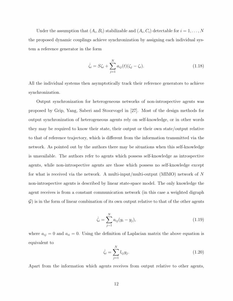


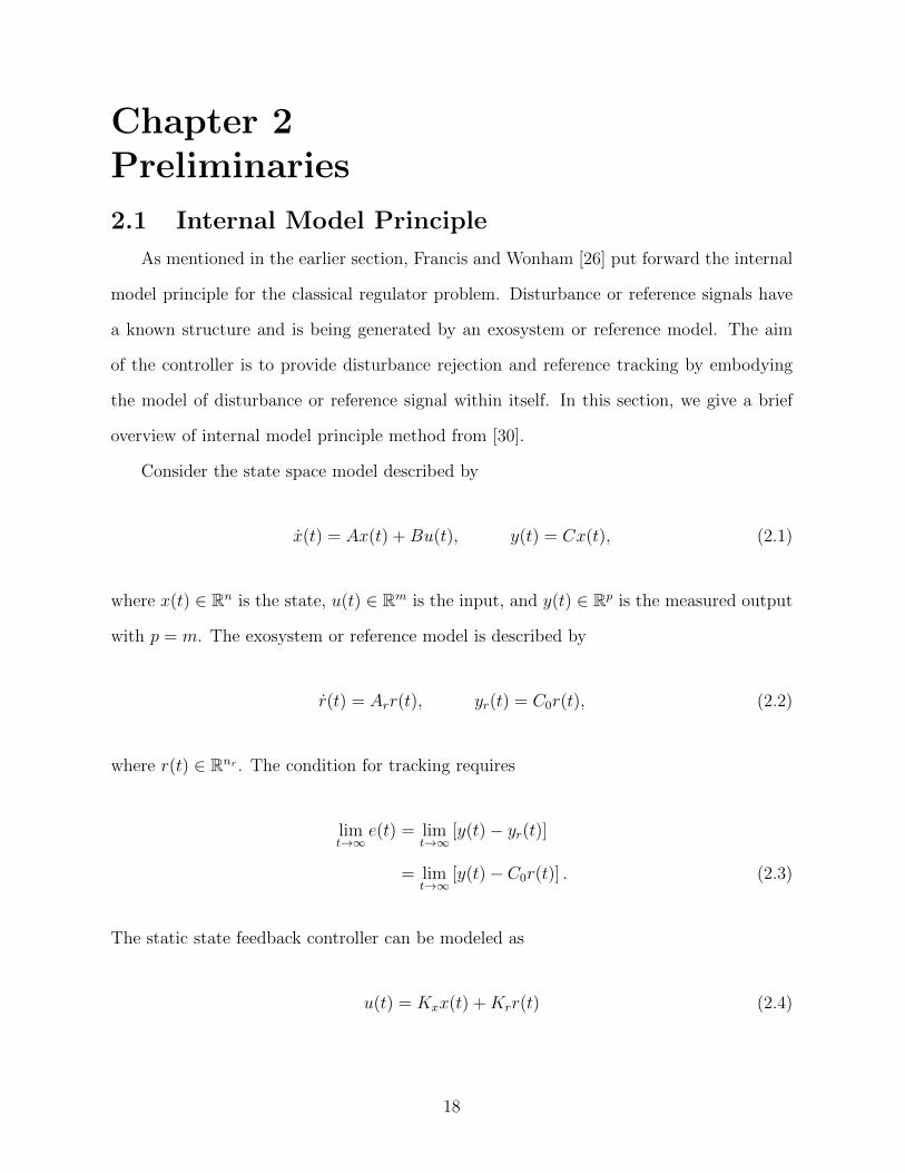
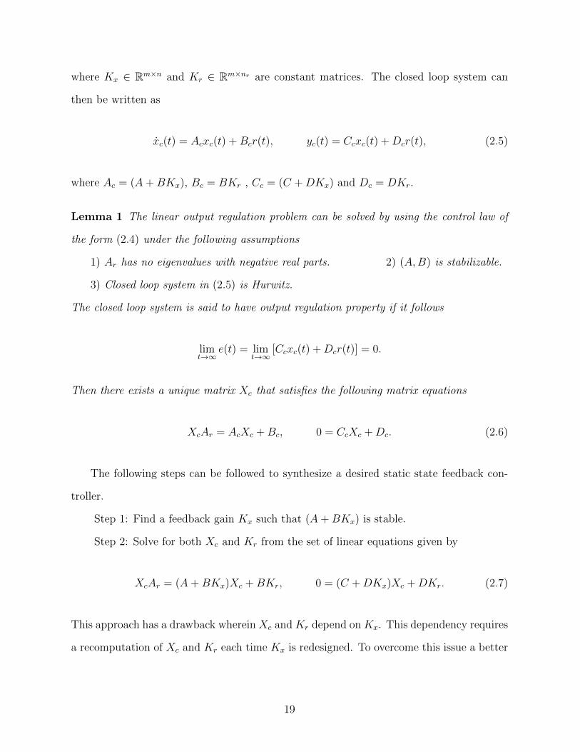


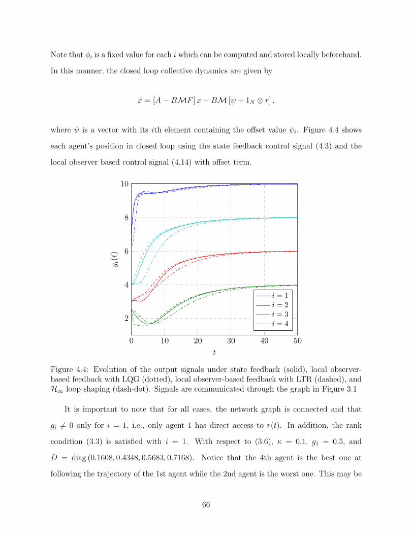


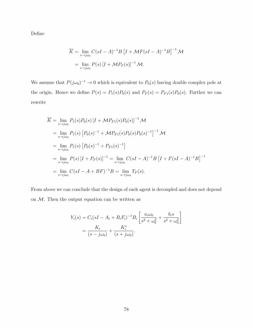

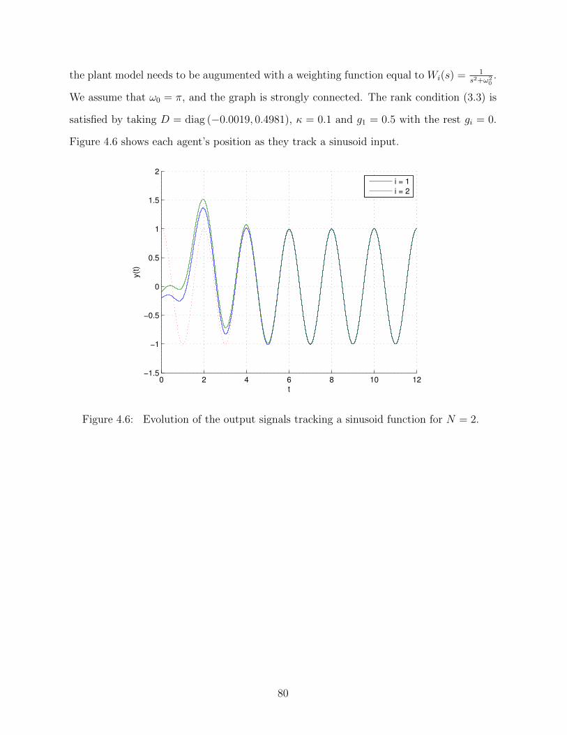


![Synchronization of Multi-Agent Systems With Heterogeneous … · 2018. 8. 20. · arXiv:1512.07362v4 [cs.SY] 13 Mar 2016 1 Synchronization of Multi-Agent Systems With Heterogeneous](https://static.documents.pub/doc/80x56/6020f60865a6e67d441a6ae2/synchronization-of-multi-agent-systems-with-heterogeneous-2018-8-20-arxiv151207362v4.jpg)