20
Output Data Analysis
| Date post: | 19-Dec-2015 |
| Category: |
Documents |
| View: | 224 times |
| Download: | 2 times |

Output Data Analysis

2
How to analyze simulation data?
• simulation
– computer based statistical sampling experiment
–estimates are just particular realizations of random variables that may
have large variances
–n independent replications
–each replication terminated by same event
– started with same initial conditions
– replications are independent by means of using different random
variables
– single measure of performance one per replication
040669 || WS 2008 || Dr. Verena Schmid || PR KFK PM/SCM/TL Praktikum Simulation I
3
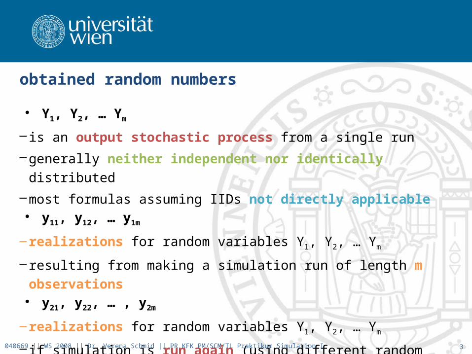
obtained random numbers
• Y1, Y2, … Ym
– is an output stochastic process from a single run
–generally neither independent nor identically distributed
–most formulas assuming IIDs not directly applicable• y11, y12, … y1m
– realizations for random variables Y1, Y2, … Ym
– resulting from making a simulation run of length m observations• y21, y22, … , y2m
– realizations for random variables Y1, Y2, … Ym
– if simulation is run again (using different random variables)
040669 || WS 2008 || Dr. Verena Schmid || PR KFK PM/SCM/TL Praktikum Simulation I
4
obtained random numbers (cont)
040669 || WS 2008 || Dr. Verena Schmid || PR KFK PM/SCM/TL Praktikum Simulation I
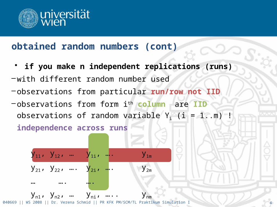
• if you make n independent replications (runs)
–with different random number used
–observations from particular run/row not IID
–observations from form ith column are IID observations of random
variable Yi (i = 1..m) ! independence across runs
y11, y12, … y1i, …. y1m
y21, y22, …. y2i, …. y2m
… …. ….
yn1, yn2, … yni, ….. ynm

5
Transient and Steady-State Behavior
• stochastic output process Y1, Y2, ..
– transient condition: Fi( y | I ) = P(Yi · y | I) for i = 1, 2…
– y is a real number
– I represents initial conditions
• density fYi
– specifies how random variable Yi can vary from one replication to
another• Fi(y | I ) ! F(y) as i ! 1
–F(y) steady-state distribution of output process Y1, Y2, …
– in theory only obtained at limit
– in practice ! finite time index (k+1) ! distributions will be approximately
the same040669 || WS 2008 || Dr. Verena Schmid || PR KFK PM/SCM/TL Praktikum Simulation I

6
Transient and Steady-State Behavior (cont.)
040669 || WS 2008 || Dr. Verena Schmid || PR KFK PM/SCM/TL Praktikum Simulation I
7
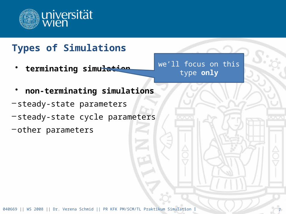
Types of Simulations
• terminating simulation
• non-terminating simulations
– steady-state parameters
– steady-state cycle parameters
–other parameters
040669 || WS 2008 || Dr. Verena Schmid || PR KFK PM/SCM/TL Praktikum Simulation I
we’ll focus on this type only

8
Example
• bank
–5 tellers, one queue
–opens at 9:00
– closes at 17:00 (stays open until all customers in the bank have been
served)
– terminating simulation• close at/after17:00 (as soon as all customers have left)
040669 || WS 2008 || Dr. Verena Schmid || PR KFK PM/SCM/TL Praktikum Simulation I

9
Example (cont.)
040669 || WS 2008 || Dr. Verena Schmid || PR KFK PM/SCM/TL Praktikum Simulation I
R # served time avg Delay avg Length % C’s delayed < 5 minutes
1 484 8.12 1.53 1.52 0.917
2 475 8.14 1.66 1.62 0.916
3 484 8.19 1.24 1.23 0.952
4 483 8.03 2.34 2.34 0.822
5 455 8.03 2.00 1.89 0.84
6 461 8.32 1.69 1.56 0.866
7 451 8.09 2.69 2.5 0.783
8 486 8.19 2.86 2.83 0.782
9 502 8.15 1.7 1.74 0.873
10 475 8.25 2.6 2.5 0.779
10
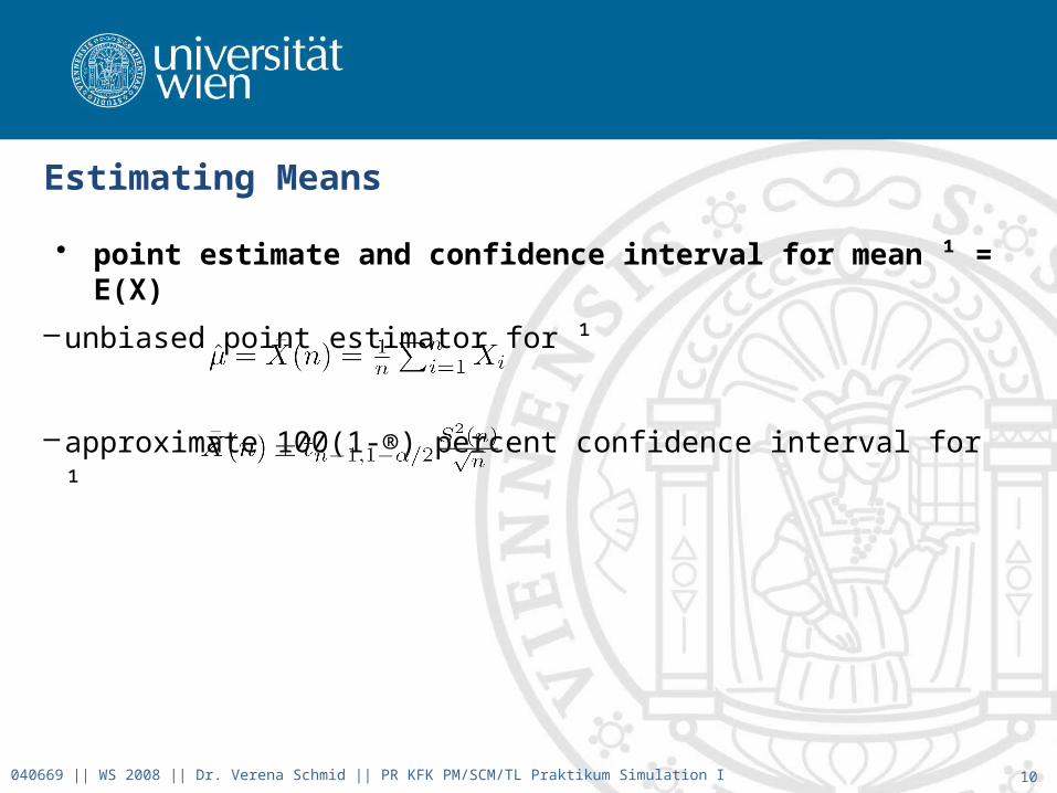
Estimating Means
• point estimate and confidence interval for mean ¹ = E(X)
–unbiased point estimator for ¹
–approximate 100(1-®) percent confidence interval for ¹
040669 || WS 2008 || Dr. Verena Schmid || PR KFK PM/SCM/TL Praktikum Simulation I

11
Estimating Means (example)
• estimate expected delay
– = 2.031
– S2(n) = 0.309
– confidence interval with ® = 10%
• estimated proportion of customers being delayed < 5 minutes
–expected proportion for a given day/run• indicator function
– = 0.853 S2(n) = 0.0039
– CI with ® = 10%040669 || WS 2008 || Dr. Verena Schmid || PR KFK PM/SCM/TL Praktikum Simulation I

12
Obtaining a desired precision
• so far
– fixed sample size procedure (based on n replications)
–disadvantage: no control over the CI’s half length (i.e. precision of )
–half length depends on population variance S2(n)
• 2 ways to measure the error in the estimate
–absolute error ¯
– relative error °
– resulting number of replications may be random
040669 || WS 2008 || Dr. Verena Schmid || PR KFK PM/SCM/TL Praktikum Simulation I
13
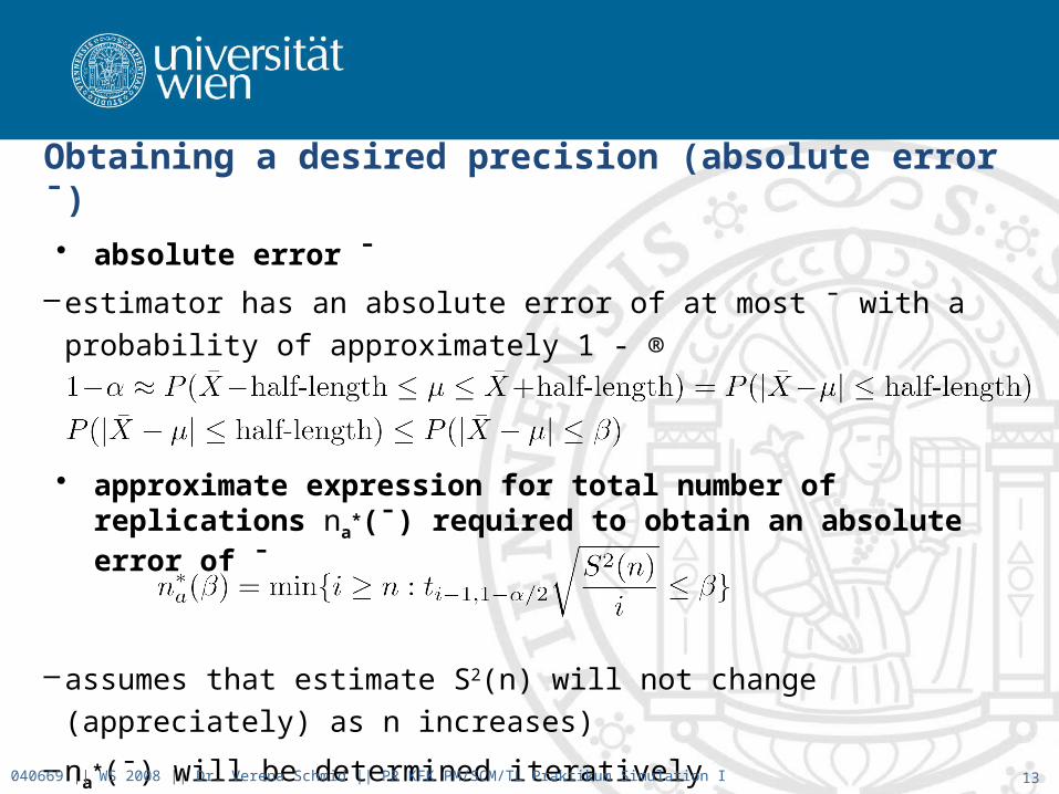
Obtaining a desired precision (absolute error ¯)
• absolute error ¯
–estimator has an absolute error of at most ¯ with a probability of
approximately 1 - ®
• approximate expression for total number of replications na*(¯)
required to obtain an absolute error of ¯
–assumes that estimate S2(n) will not change (appreciately) as n
increases)
–na*(¯) will be determined iteratively
040669 || WS 2008 || Dr. Verena Schmid || PR KFK PM/SCM/TL Praktikum Simulation I
14
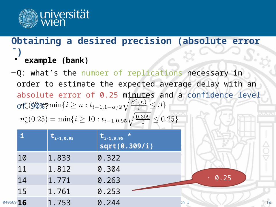
Obtaining a desired precision (absolute error ¯) • example (bank)
–Q: what’s the number of replications necessary in order to estimate the
expected average delay with an absolute error of 0.25 minutes and a
confidence level of 90%?
040669 || WS 2008 || Dr. Verena Schmid || PR KFK PM/SCM/TL Praktikum Simulation I
i ti-1,0.95 ti-1,0.95 * sqrt(0.309/i)
10 1.833 0.32211 1.812 0.30414 1.771 0.26315 1.761 0.25316 1.753 0.244
· 0.25
15
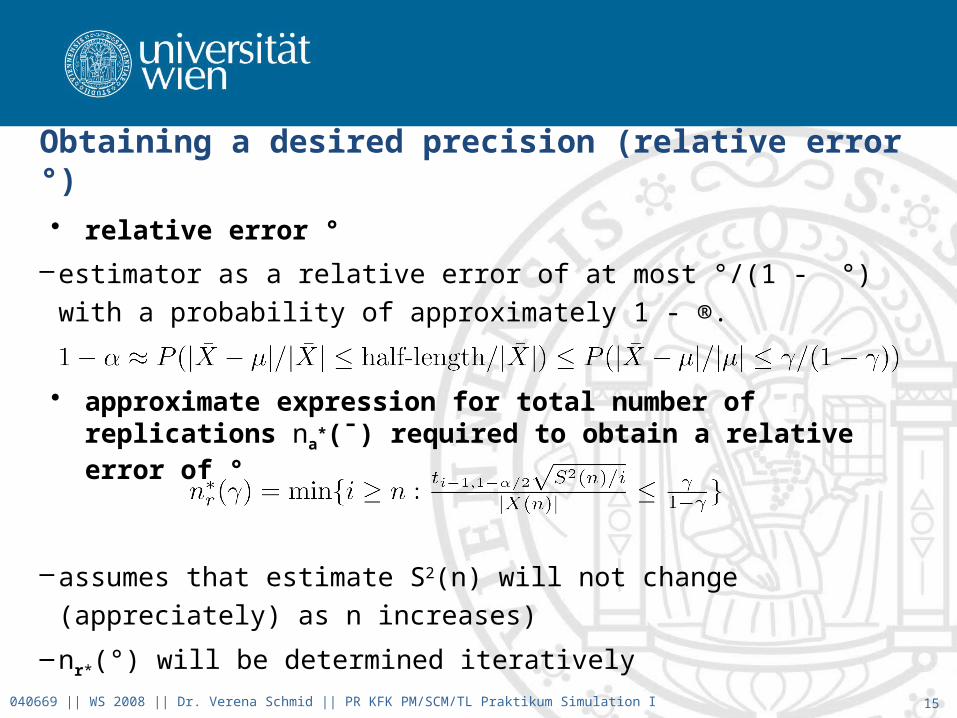
Obtaining a desired precision (relative error °)
• relative error °
–estimator as a relative error of at most °/(1 - °) with a probability of
approximately 1 - ®.
• approximate expression for total number of replications na*(¯)
required to obtain a relative error of °
–assumes that estimate S2(n) will not change (appreciately) as n
increases)
–nr*(°) will be determined iteratively
040669 || WS 2008 || Dr. Verena Schmid || PR KFK PM/SCM/TL Praktikum Simulation I
16
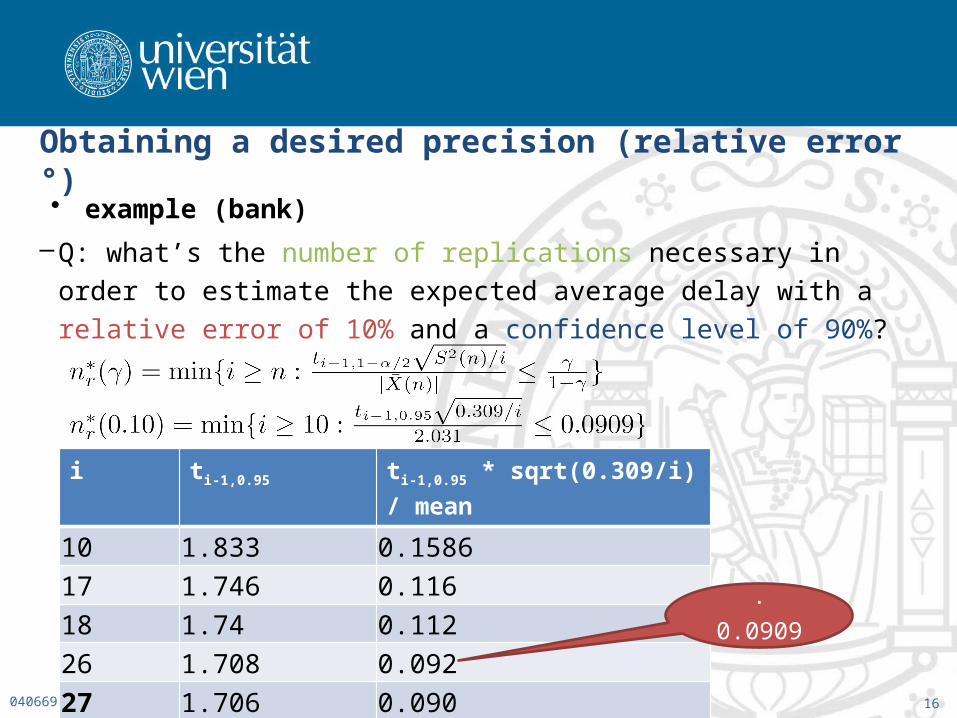
Obtaining a desired precision (relative error °) • example (bank)
–Q: what’s the number of replications necessary in order to estimate the
expected average delay with a relative error of 10% and a confidence
level of 90%?
040669 || WS 2008 || Dr. Verena Schmid || PR KFK PM/SCM/TL Praktikum Simulation I
i ti-1,0.95 ti-1,0.95 * sqrt(0.309/i) / mean
10 1.833 0.158617 1.746 0.11618 1.74 0.11226 1.708 0.09227 1.706 0.090
· 0.0909
17
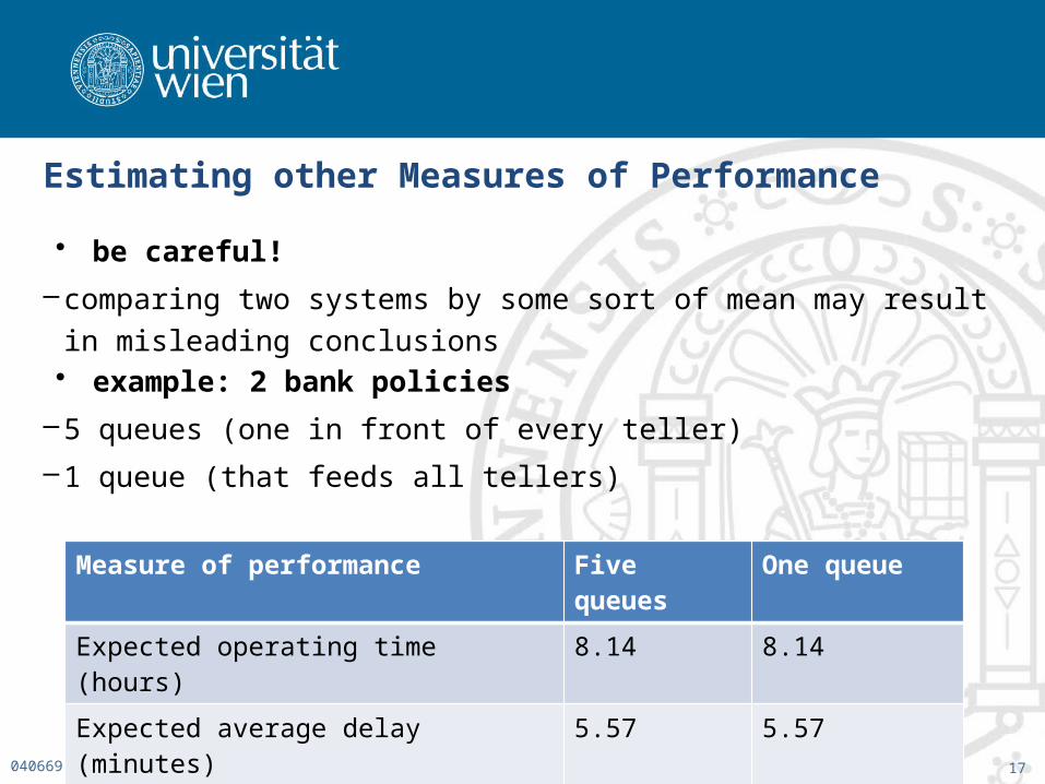
Estimating other Measures of Performance
• be careful!
– comparing two systems by some sort of mean may result in misleading
conclusions• example: 2 bank policies
–5 queues (one in front of every teller)
–1 queue (that feeds all tellers)
040669 || WS 2008 || Dr. Verena Schmid || PR KFK PM/SCM/TL Praktikum Simulation I
Measure of performance Five queues One queue
Expected operating time (hours) 8.14 8.14
Expected average delay (minutes) 5.57 5.57
Expected average number in queue(s) 5.52 5.52

18
Estimating other Measures of Performance
• Estimates of expected proportions of delays in interval
040669 || WS 2008 || Dr. Verena Schmid || PR KFK PM/SCM/TL Praktikum Simulation I
Interval (minutes) Five queues One queue
[0,5) 0.626 0.597
[5,10) 0.182 0.188
[10,15) 0.076 0.107
[15,20) 0.047 0.095
[20,25) 0.031 0.013
[25,30) 0.02 0
[30,35) 0.015 0
[35,40) 0.003 0
[40,45) 0 0
still identical?
19
Choosing initial conditions
• careful!
–measures of performance depend explicitly on the state of the system
at time 0
– take care when choosing appropriate initial conditions
• example: estimate expected average delay at bank between noon and 1pm
–bank will probably be quite congested at noon• starting with no customers present -> estimates will be biased low
040669 || WS 2008 || Dr. Verena Schmid || PR KFK PM/SCM/TL Praktikum Simulation I
20
Choosing initial conditions
• careful!
–measures of performance depend explicitly on the state of the system
at time 0
– take care when choosing appropriate initial conditions
• 2 heuristic approaches
–use warmup period
–collect data to get an idea of state of system and choose it randomly
040669 || WS 2008 || Dr. Verena Schmid || PR KFK PM/SCM/TL Praktikum Simulation I


