DI

SC

US

SI

ON

P

AP

ER

S

ER

IE

S

Forschungsinstitut zur Zukunft der ArbeitInstitute for the Study of Labor

Outsourcing and Technological Change

IZA DP No. 4678

December 2009

Ann BartelSaul LachNachum Sicherman

Outsourcing and Technological Change

Ann Bartel Columbia University and NBER

Saul Lach

Hebrew University and CEPR

Nachum Sicherman Columbia University and IZA

Discussion Paper No. 4678 December 2009

IZA

P.O. Box 7240 53072 Bonn

Germany

Phone: +49-228-3894-0 Fax: +49-228-3894-180

E-mail: iza@iza.org

Any opinions expressed here are those of the author(s) and not those of IZA. Research published in this series may include views on policy, but the institute itself takes no institutional policy positions. The Institute for the Study of Labor (IZA) in Bonn is a local and virtual international research center and a place of communication between science, politics and business. IZA is an independent nonprofit organization supported by Deutsche Post Foundation. The center is associated with the University of Bonn and offers a stimulating research environment through its international network, workshops and conferences, data service, project support, research visits and doctoral program. IZA engages in (i) original and internationally competitive research in all fields of labor economics, (ii) development of policy concepts, and (iii) dissemination of research results and concepts to the interested public. IZA Discussion Papers often represent preliminary work and are circulated to encourage discussion. Citation of such a paper should account for its provisional character. A revised version may be available directly from the author.

IZA Discussion Paper No. 4678 December 2009

ABSTRACT

Outsourcing and Technological Change* We present a dynamic model where the probability of outsourcing production is increasing in the firm’s expectation of technological change. As the pace of innovations in production technologies increases, the less time the firm has to amortize the sunk costs associated with purchasing and adopting new technologies to produce in-house. Therefore, purchasing from market suppliers, who can afford to use the latest technology, becomes relatively cheaper. The predictions of the model are tested using a panel dataset on Spanish firms for the time period 1990 through 2002. In order to address potential endogeneity problems, we use an exogenous proxy for technological change, namely the number of patents granted by the U.S. patent office classified by technological class. We map the technological classes to the Spanish industrial sectors in which the patents are used and provide causal evidence of the impact of expected technological change on the likelihood and extent of production outsourcing. No prior study has been able to provide such causal evidence. Our results are robust to the inclusion of detailed characteristics of the firms as well as firm fixed effects. JEL Classification: J21, L23, L24, O33 Keywords: outsourcing, technological change Corresponding author: Nachum Sicherman Graduate School of Business Columbia University New York, NY 10027 USA E-mail: Nachum.Sicherman@Columbia.edu

* The authors gratefully acknowledge the generous support of grants from the Columbia University Institute for Social and Economic Research and Policy, Columbia Business School’s Center for International Business Education and Research, and the European Commission (Grant # CIT5-CT-2006-028942). We thank Diego Rodriguez Rodriguez for his assistance with the ESSE data and Daniel Johnson for providing us with his algorithm for converting patent data from industry of origin to industry of use. We received very helpful comments from Maria Guadalupe, Catherine Thomas and participants in the February 2009 “Innovation, Internationalization and Global Labor Markets” Conference in Torino, Italy. Outstanding research assistance was provided by Ricardo Correa, Cecilia Machado and Raymond Lim.

2

I. Introduction

Outsourcing, or the contracting out of activities to subcontractors outside the firm, has

become widespread in many countries.1 A number of explanations for the increase in outsourcing

have been proposed and tested in the literature. Among them are that outsourcing is a response to

unpredictable variations in demand (Abraham and Taylor, 1996), an opportunity to take

advantage of the specialized knowledge of suppliers (Abraham and Taylor, 1996), and a method

to save on labor costs (Abraham and Taylor, 1996; Autor, 2001; Diaz-Mora, 2005; and Girma and

Gorg, 2004).2

Another important determinant of outsourcing is technology and this has been the subject

of theoretical and empirical work. According to the transactions costs theory (Williamson 1975,

1985), if investments result in greater asset specificity, firms fearing expropriation of investments

will reduce outsourcing. The property rights theory (Grossman and Hart, 1986) predicts that

vertical integration between an upstream firm (the supplier) and a downstream firm (the final

good producer) generates different costs and benefits to each of the parties. Therefore, the

incentives to integrate or to outsource depend on which investments – the supplier’s or the final

good producer’s – are relatively more important for the success of the joint relationship

(Grossman and Hart, 1986; Gibbons, 2005; Hubbard, 2008).3

Some empirical studies have focused on testing these theories. In a study of U.K.

manufacturing firms, Acemoglu et.al. (2010) found evidence consistent with the predictions of

1 See Arndt and Kierzkowski (2001), Girma and Gorg (2004), Mol (2005), Magnani (2006) and Abramovsky and Griffith (2006). 2 Other researchers (Ono (2007) and Holl (2008)) have studied the effect of agglomeration economies on outsourcing. For empirical studies of the impacts of outsourcing on wages and productivity, see Feenstra and Hanson (1999), Amiti and Wei (2006), Gorg, Hanley and Strobl (2007), Gorg and Hanley (2007), and Lopez (2002). 3 Grossman and Helpman (2003, 2005) and Antras (2005a, 2005b) use the insights of the property rights theory to study important issues in international trade such as the decision to obtain intermediate inputs by engaging in foreign direct investment or contracting with arm’s-length overseas suppliers.

3

the property rights theory, namely that technology intensity in the producing industry is

associated with more vertical integration while technology intensity in the supplying industry is

associated with less integration, where technology intensity is measured by R&D intensity.

Lileeva and Van Biesebroeck (2008) also found evidence consistent with the predictions of the

property rights model, using data on Canadian manufacturing firms. Mol (2005), however, found

that in the Dutch manufacturing sector, R&D-intensive industries were able to solve the non-

contractibility problem by using partnership relations with outside suppliers to reduce the

likelihood of specific investments being appropriated.4 Other studies that have examined the

relationship between technology and outsourcing, without relying on the transactions cost or

property rights theories, are Magnani (2006) who found evidence that technological diffusion

driven by R&D spillovers was in part responsible for the growth of outsourced services in the

U.S. and Abramovsky and Griffith (2006) who found that UK firms that were intensive in

information and communication technologies were more likely to purchase services in the

market.

In this paper we provide an alternative perspective on the relationship between

technology and outsourcing. Unlike previous studies which have focused on the nature or

intensity of technology, we focus on expectations of technology change. We present a dynamic

model that analyzes how firms’ expectations with regards to technological change influence the

decision to outsource production, an issue ignored in the literature.5 Our model abstracts from

other considerations such as transactions costs or asset specificity. The model shows that

outsourcing becomes more beneficial to the firm when technology is changing rapidly. A firm

4 Baker and Hubbard (2003) consider how information technology in the trucking industry impacts contracting possibilities and vertical integration. Baccara (2007) uses a general equilibrium model to study how information leakages could affect a firm’s outsourcing decision as well as its investments in R&D. 5 Lewis and Sappington (1991) present a model in which technological progress acts to reduce the cost asymmetries between suppliers and end users. In their model, technological progress reduces the suppliers’ cost advantage, thereby making outsourcing less likely. Unlike Lewis and Sappington, our model does not consider the nature of technology but focuses instead on the rate of change of the technology.

4

can buy the latest technology and produce intermediate inputs in-house. Firms incur a sunk cost

when adopting new technologies. Outsourcing, on the other hand, enables the firm to purchase

inputs from supplying firms using the latest production technology while avoiding the sunk costs

of the new technology. As the pace of innovations in production technology increases, the less

time the firm has to amortize the sunk costs associated with purchasing the new technologies.

This makes producing in-house with the latest technologies relatively more expensive than

outsourcing. The model therefore provides an explanation for the recent increases in outsourcing

that have taken place in an environment of increased expectations for technological change.

We test the predictions of the model using a panel dataset of Spanish firms for the time

period 1990 through 2002. This dataset is superior to those used in previous studies of the

determinants of outsourcing in several dimensions.6 First, unlike many studies that used industry

level data, we use a large sample of firms. Second, we have panel data that allow us to observe

changes within firms over a long time period. Third, in addition to detailed information on

outsourcing, the dataset provides rich information related to technological activities, such as the

use of computers, investment in R&D, registration of patents, and product innovation.

While information on the firm’s technological activities is likely to be correlated with the

firm’s expectations of technological change, these variables cannot be treated as purely

exogenous. To address this endogeneity problem, we use the number of patents granted by the

U.S. patent office classified by technological class and map the technological classes to the

Spanish industries in which the patents are used.7 The empirical results support the main

prediction of the theoretical model, namely, that all other things equal, outsourcing increases with

the probability of technological change. Our use of the patent variable enables us to conclude

that this relationship is causal; no prior study has been able to provide causal evidence of the

6 Holl (2008) used this dataset to study the effect of agglomeration economies on outsourcing and Lopez (2002) used it to study the impact of outsourcing on wages. 7 Patents are commonly classified by the industry in which they originated, while our analysis calls for a classification by industry of use. In Section III we describe how we constructed such a measure.

5

impact of technological change on outsourcing. We also show that our results are robust to the

inclusion of a measure of relationship-specific investments and furthermore that the patents

variable remains significant when the analysis is restricted to industries with little relationship-

specific investments. Importantly, this shows that our results cannot be explained by the

transactions cost or property rights theories. Finally, our finding regarding the relationship

between patents and outsourcing is robust to the inclusion of firm-level fixed effects, unlike the

findings for many of the non-technology variables that prior researchers have studied.

Part II describes a simple dynamic model of the relationship between outsourcing and

expected technological change. The complete model is given in the Appendix. Part III discusses

the data and empirical specifications used to test the predictions of the model. Results are

presented in Part IV. Part V concludes.

II. The Decision to Outsource Production

In this section we present a simple model that shows how the decision to outsource

production is related to the probability of technological change. The complete model is presented

in the Appendix. The model is motivated with the following example.

Suppose that the production of a final good requires an input that is composed of

advanced capital equipment and labor. This input can either be produced in-house by the final

good firm or it can be purchased in the market from an external supplier. The latter option

amounts to outsourcing the production process. Installing the capital equipment and training the

workforce to use the equipment involve expenses that are sunk to the firm. Suppose that

technological change occurs in the sector supplying capital goods to this firm. For example, new

IT-enhanced capital equipment becomes available for use in manufacturing.8 The firm will need

8 For example, in many manufacturing industries, computer numerically controlled (CNC) machines replaced numerically controlled machines which had previously replaced manual machines. See Bartel, Ichniowski and Shaw (2007) for a discussion of the impact of these new technologies on productivity in the valve-making industry.

6

to decide between making this capital investment or outsourcing the production of the final good

to a firm that uses the new equipment. The relative costs of in-house production will increase if

the frequency of technological change is increasing because the length of time over which a given

fixed investment will benefit the firm becomes too short to justify incurring the sunk costs

associated with the investment, making outsourcing the cheaper alternative.9 The model we

present below captures the essence of this example.

A firm produces a profit-maximizing amount q of a final good using a single input .x

The model focuses on determining how to procure a given level of input .x There are two ways

of obtaining .x One way is to produce x in-house, while the other way is to buy x in the

market, which we refer to as "outsourcing production" . We implicitly assume that there are firms

(the suppliers) willing to produce and supply x , i.e., there is an active market for x but we do

not model the supply side here. The final good producer takes the price of x as given.

For simplicity we assume constant returns to scale in production. This allows us, after a

normalization, to set =x q which is desirable for the empirical work since q is observed. This

assumption also ensures that the firm does not split x between in-house production and

outsourcing. The firm will either produce all of x in-house or will outsource all of it.10 Let

= 1ty indicate that the firm decides to outsource x in period ,t while = 0ty indicates in-house

production of x .

9 The firm could also attempt to lower its sunk costs by outsourcing the training of its workforce. For example, the firm may need to hire an instructor to train a single operator of the advanced equipment, but the same instructor could probably train more than one person simultaneously without incurring additional costs. The combination of a sunk cost and indivisibility (of the instructor) is precisely the feature being exploited by temporary employment agencies (Autor, 2001): they use the same instructor to train several workers in basic computer skills and offer them to firms at an attractive price because they can spread the sunk cost over a larger output (computer-skilled workers). Our model and empirical work does not consider outsourcing of training but rather focuses on the outsourcing of production. 10In reality, however, firms usually outsource part of their production, so that we should interpret x as one of the multiple input components of the final output.

7

In order to produce x in-house the firm uses another input which we call “machines" ,

each of which produces tθ units of .x The productivity parameter θ evolves over time in a

discrete fashion. That is, with probability ,λ θ can jump to +θ δ in the next period,

1

with probability =

with probability 1

θ δ λθ

θ λ+

+⎧⎪⎨⎪ −⎩

t

t

t

where > 0.δ

Our goal is to show how the decision to outsource depends on ,λ the probability of

technological change. Note that technological change occurs in the sector producing the machines

used in the production of .x Thus, we view technological change as embodied in machines.

The revenues obtained from selling the final good do not depend on the way in which x

was procured. Thus, the decision to produce x in-house or to buy it in the market (outsource it )

depends on which alternative is cheaper. At the beginning of each period, the state of technology

is realized and the firm compares the costs of in-house production ( 0 )C to the costs of

outsourcing 1( )C .

Adopting a new technology involves the payment of 0≥s dollars to use it. The sunk

cost s is associated with installing and using the machines of a given productivity for the first

time. s is incurred only once and includes training costs. For simplicity, this sunk cost does not

depend on the firm's previous experience with in-house production. Thus, there are no dynamic

gains associated with in-house production.

When a new technology appears in the market a firm that decides to produce in-house

can, in principle, always " skip" the new, upgraded machines. That is, the firm has the option to

continue using the previous (old) technology if it has bought it in the past, or it could even buy

8

the old technology in the market if it did not do so previously. It is not always profitable to adopt

the latest technology. This adoption decision depends on whether using the upgraded technology

is less costly than using the old technology. This is determined by the size of the sunk cost

relative to the savings of using the latest technology. However, to simplify the analysis and

because this adoption decision is not the focus of the paper, we will assume that upgrading

always dominates keeping the old technology (and, as shown in the Appendix, we make the

necessary assumptions that guarantee this is the optimal decision). Thus, if a firm decides to

produce in-house it will always do so using the latest technology.

The cost of in-house production 0C is therefore the cost of production using the latest

technology available. A-fortiori, this assumption logically implies that suppliers of x in the

market should always be producing with the latest technology because they spread the sunk cost

of upgrading over a larger quantity of output. Thus, outsourcing involves buying x from

suppliers using the latest technology.

The cost of in-house production 0C depends on whether technology changed from last

period and on the firm’s outsourcing decision last period, 1.−ty If technology changed, the firm

will pay the sunk cost s and other costs of production to produce q units of .x If there was no

change in technology the firm does not need to pay s again if it already produced in-house last

period 1( = 0)−ty but, if it did outsource last period 1( = 1),−ty it will have to pay s to produce

in-house with the latest technology (the one existing last period). Thus, 01 1( , , , , ).− −t t tC y s qθ θ

The cost of outsourcing 1C depends on the market price of x which can vary with

technology but it does not depend on 1.−ty The price of x , as well as the prices of the machines,

9

may depend on the state of technology θ, as shown in the Appendix, but to simplify the notation

here we do not condition on prices explicitly. Thus, 11( , , ).−t tC qθ θ 11

At the beginning of each period ,t the firm observes the evolution of technology up to ,t

i.e., 1 2( , , , )− − Kt t tθ θ θ and its past actions ( 1 2,, ),− − Kt ty y as well as the sunk cost s and the level

of output q it wants to produce. The firm makes its (discrete) outsourcing decision in order to

maximize the expected discounted value of its profits. Note that the Markovian nature of

technology implies that only tθ affects the future evolution of technology. However, because the

costs of procuring x depend on whether tθ is a new technology and on whether it was previously

used or not 1( )−ty , the firm bases its outsourcing decision at t also on 1−tθ and 1.−ty

Let 1 1( , , , , )− −t t tV y s qθ θ be the expected discounted value of the firm's stream of profits

given 1 1( , , , , ).− −t t ty s qθ θ V is defined by,

{ }0 11 1 1 1 1 1( , , , , ) = ( , , , , ), ( , , , , )− − − − − −t t t t t t t t tV y s q Max V y s q V y s qθ θ θ θ θ θ (1)

where 0V is the expected discounted value if the firm decides to produce in-house

during ,t i.e., = 0,ty and 1V is defined similarly when the firm decides to outsource, i.e.,

= 1.ty

The firm decides to outsource if, and only if,

1 01 1 1 1= 1 ( , , , , ) ( , , , , ) 0− − − −⇔ − ≥t t t t t t ty V y s q V y s qθ θ θ θ (2)

11 In the formal model we also add other factors that affect the cost of outsourcing that are known to the firm but unobserved to the econometrician. These factors reflect adjustment costs due to loss of control over the input design, i.e., the additional cost of using a standardized input. This additional cost is absent when x is produced in-house because the firm can perfectly tailor the input to its specific needs.

10

In the Appendix we solve for 1 0−V V which completely determines the firm's

outsourcing decision in period t as a function of ( )1 1, , , , .− −t t ty s qθ θ This implies that there is a

threshold value for the sunk cost s such that firms with s below the threshold produce in-house

while those with sunk costs above the threshold outsource in period .t

This threshold value depends on the state variables as well as on the parameters of the

model. We are interested in how the threshold value changes with .λ In the Appendix we show

that the threshold value decreases with λ (for any value of the state) and therefore firms facing

higher expectations of technological change in their inputs -- a higher λ -- are more likely to

outsource, all other things equal.12 Thus, when λ increases and new production technologies are

more likely to appear in the future, firms will be more reluctant to buy the current machines today

and produce in-house because these technologies will soon be obsolete. Upgrading the

technology -- which is the optimal thing to do -- involves incurring a sunk cost di novo. The

higher is ,λ the more frequently the new machines arrive and the less time the firm has to

amortize the sunk costs. Instead, the firm can use outsourcing to obtain x from supplying firms

using the latest technology and avoid the sunk costs. All other things equal, an increase in λ

decreases the cost of outsourcing relative to that of in-house production making the firm more

likely to outsource. This is the main prediction of the model that we take to the data .

III. Data and Empirical Specification

We use data for 1990-2002 from the Encuesta sobre Estrategias Empresariales (ESEE, or

Survey on Business Strategies), a survey of 3,195 Spanish manufacturing firms conducted by the

Fundacion SEPI with the support of the Ministry of Industry, Tourism and Trade. The survey has 12In addition, larger firms and firms facing higher adjustment costs from outsourcing also have higher probabilities of producing in-house.

11

been conducted annually since 1990 and is an unbalanced panel. In 1990, all firms with more than

200 employees were asked to participate in the survey (with a response rate of 70 percent). Firms

with 10-200 employees were chosen according to a random sampling scheme. In subsequent

years, as firms dropped from the survey, new firms were incorporated into the sample using the

same sampling criteria as in the base year. There are approximately 1800 firms in each year of the

survey.

The survey includes annual information on firms’ production outsourcing decisions,

defined as a contractual relationship in which the firm commissions a third party to produce

products, parts, or components made to the firm’s specifications.13 We use this information to

create two indicators of production outsourcing: a dummy for whether or not the firm engaged in

outsourcing, and the value of outsourcing divided by total costs. Total costs are defined as the

sum of: (1) labor costs, (2) the cost of external services (R&D, advertising, public relations and

other) and (3) purchases of goods for sale in the same condition in which they were acquired, raw

materials and other consumables, and work carried out by subcontractors. The items in (3) are

reported in the survey as an aggregate figure.

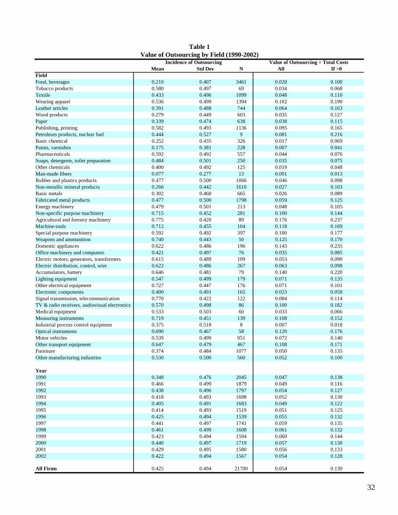
Table 1 shows the percentage of firms that reported outsourcing at least some part of

production during the 1990 – 2002 time period and the mean value of the outsourced production

as a percentage of total cost. On average, 43% of firms reported that they outsourced production

during this time period. The outsourcing percentage rose from 35% in 1990 to 42% in 2002, with

even higher values in some of the intervening years. There is significant variation in the

likelihood of outsourcing across industries ranging from a low of 7.7% for “man-made fibers” to

a high of 77.5% for “agricultural and forestry machinery”. The average value of the outsourced

production as a percentage of total costs is 5.4 percent during this time period; for firms that did

outsource production, the mean value of outsourced production as a percentage of total costs is 13

13 Production outsourcing does not include purchases of non-customized products, parts or components.

12

percent, with a low of 1.8 percent (industrial process control equipment) and a high of 23.7

percent (agricultural and forestry machinery).

The model in the Appendix derives the decision to outsource, yit , as a function of

expected technological change, λ, size of the firm (output or sales), lagged outsourcing and input

prices. Under the assumption that input prices are common to all firms in an industry, these will

be captured by industry dummies (ID). The main implication of the model presented in Part II is

that, all other things equal, the probability of outsourcing increases with the exogenous

probability of technological change, λ, which is given to the firm and represents the probability of

technological change in the production process. The model also predicts that the probability of

outsourcing decreases with sales, qt.

As a first approximation to the model, we estimate equation (3):

= + + +∑it it it j ij itj

y q ID uβ λ α δ (3)

where the dependent variable is either of the two measures of outsourcing. Later, we add

dynamics to this equation.

In order to test the main prediction of the model, we need a proxy for λ, the firm’s

expectations with regard to technological change in its production process. The Spanish dataset

includes a number of variables which might be reasonable proxies for λ. The firm’s investment in

R&D or its patent registrations can be good proxies to the extent that R&D (or patenting) is used

to adapt exogenous changes in the production technology to the specific requirements of the firm.

The notion of R&D serving this adaptive role has been tested by Cohen and Leventhal (1989).

Another suitable proxy could be whether the firm engages in product innovation since this may

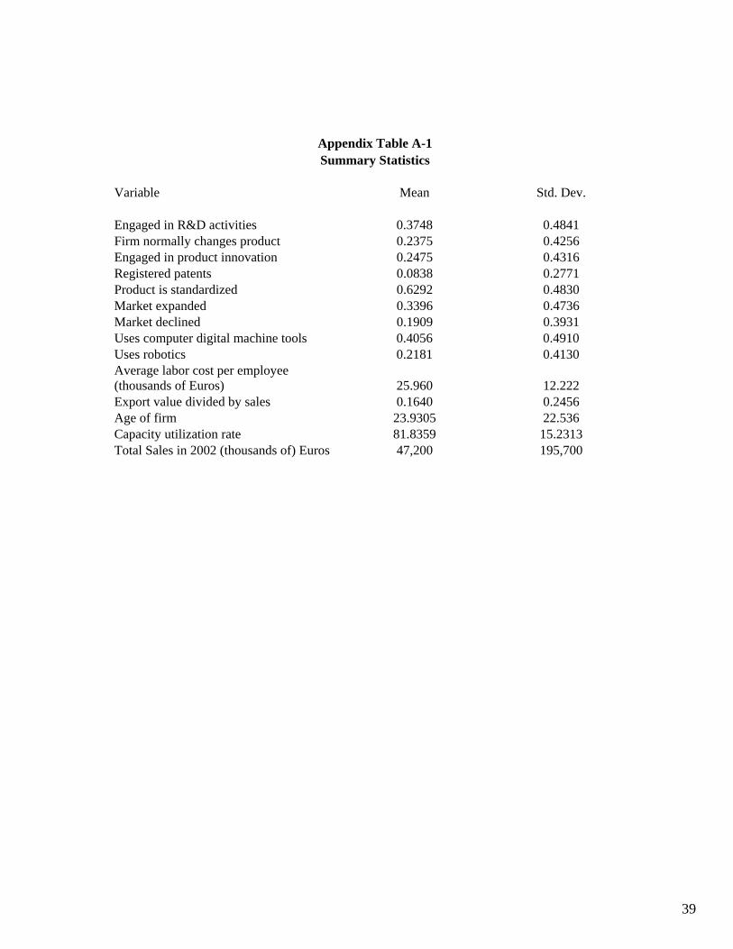
be facilitated by exogenous changes in production technologies. Summary statistics for R&D

13

intensity, patent registrations, and product innovation are shown in Appendix Table A-1. While

these variables are likely to be correlated with the firms’ expectations of technological change in

its production process, they could be endogenous if unobserved factors drive these decisions as

well as the decision to outsource. For example, firms that are unobservably more “innovative” or

“creative” may be engaging in more R&D, registering patents, engaging in product innovations

and outsourcing production.

We can partially address this concern by exploiting the panel nature of our data which

allows us to control for time-invariant unobserved factors that affect both the decision to engage

in R&D (and therefore increase λ) and to outsource. Inclusion of fixed effects also enables us to

control for other factors that affect the cost of outsourcing such as adjustment costs due to loss of

control over input design. But adding fixed effects does not address all sources of endogeneity of

the proposed proxies for λ. Causality could also go in the other direction. For example, the

decision to outsource could induce the firm to shift from secrecy to patenting in order to protect

an innovation.14

In order to address this concern, we use a proxy for λ which, by construction, is

exogenous to the firm. This proxy is the number of patents granted yearly by the U.S. Patent

Office that are linked to the industry in which the patents are used. These data are obtained from

the NBER Patent Citations Data File described in Hall, Jaffe and Trajtenberg (2001). The

industrial sector to which a patent is assigned is usually not identical to the sector using the

patented invention. Hence it is necessary to convert data on the number of patents originating in

an industry into the number of patents used by an industry. We are able to do this conversion

using an algorithm kindly provided by Daniel Johnson as described in Johnson (2002). This

algorithm takes the data on patents originating in the U.S. in each year and creates a count of the

number of patents used by each of 38 manufacturing sectors (based on the ISIC classification). 14 For this reason, technological change might deter firms from outsourcing the production of a product or component for which competitors could more easily copy or steal an innovation (Williamson, 1985).

14

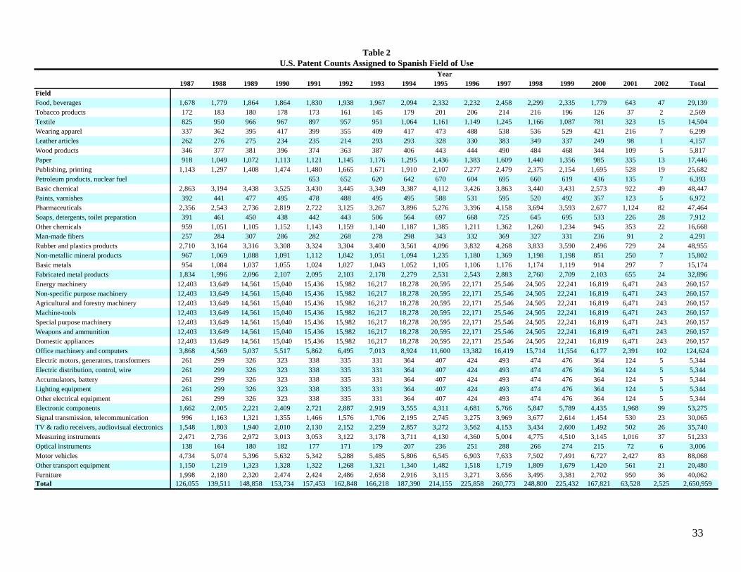
We then matched these 38 sectors to the 44 manufacturing sectors used in the ESEE. Table 2

shows the contemporaneous patent counts for 1990 through 2002 assigned to each of the Spanish

manufacturing sectors. The patent counts for the later years are significantly lower than those in

earlier years because of the time lag between submission of a patent application and the actual

granting of the patent. Note that seven industries (energy machinery, non-specific-purpose

machinery, agricultural and forestry machinery, machine-tools, special purpose machinery,

weapons and ammunition, and domestic appliances) were assigned the same patent counts

because the ISIC classification groups these industries together.

For the regressions, we calculated, for each year, the average number of patents used in

the sector over the previous three years and assigned this value to each Spanish firm based on its

industrial sector. The three period lag is used instead of the contemporaneous value of patents for

two reasons. First, year to year variations in patents are volatile and using information over a

three year period smooths the data.15 Second, given the time lag between patent application and

patent granting, using the average of patent counts over the prior three years, rather than the

current year plus the prior two years, enables us to include 2002 in our analysis. The U.S. patents

variable is clearly exogenous to the outsourcing decisions of the Spanish firm and enables us to

estimate the causal impact of expected technological change on outsourcing.

Our model predicts that larger firms will be less likely to outsource and we therefore

include the firm’s sales in the equation. We also control for a set of variables that have been the

subject of previous research on the determinants of outsourcing. Since firms may use outsourcing

as a way of economizing on labor costs (see Abraham and Taylor, 1996), we include the firm’s

average labor cost defined as total annual spending (wages and benefits) on employees divided by

total employment. Outsourcing may also be used to smooth the workload of the core workforce

during peaks of demand (Abraham and Taylor, 1996; Holl, 2008). Hence, we add a measure of

capacity utilization defined as the average percentage of the standard production capacity used 15We tried shorter and longer time horizons and our results were unchanged.

15

during the year. Another factor that can increase the propensity to outsource is the volatility in

demand for the product (Abraham and Taylor, 1996; Holl, 2008). We proxy volatility using two

dummy variables that indicate whether the company’s main market expanded or declined during

the year. It has also been argued that very young firms may be less likely to outsource because

they have not had sufficient time to learn about the quality and reliability of potential

subcontractors (Holl, 2008) and we therefore include the age of the firm. Whether the firm

primarily produces standardized products or custom made products could also affect the

propensity to outsource production if custom made products involve more frequent changes in the

production process. We add a dummy variable that equals one if the firm indicated that it

produces standardized products that are, in most cases, the same for all buyers. Finally, we

control for the firm’s export propensity, the value of exports divided by sales (Girma and Gorg,

2004; Diaz-Mora, 2005; and Holl, 2008).16 Summary statistics on all of these variables are shown

in Appendix Table A-1.

IV. Results

We use two dependent variables, an indicator of whether the firm is engaged in

outsourcing production and the value of the firm’s outsourced production as a percentage of total

costs. Regressions using the first dependent variable are estimated with fixed effect Logit while

random effect Tobit is used for the second dependent variable since 60 percent of the

observations are zeroes. Table 3 uses the proxies for expected technological change that come

directly from the Spanish data (whether the firm engaged in R&D, registered patents or

introduced new products) while Tables 4 and 5 use the exogenous measure of expected

technological change based on the U.S. patent filings.

16 The firm’s location could also serve as a proxy for the ease with which outsourcing can be done (see Ono, 2007). Our data do not provide this information, but a firm’s location is likely to be time-invariant and its potential effect on outsourcing is captured by the firm fixed effect in our regressions.

16

A. Expected Technological Change

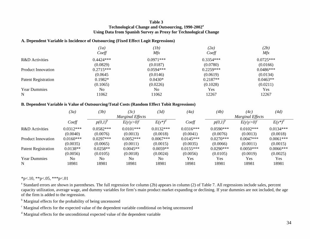
Table 3 shows the coefficients on the technological change proxies from fixed effect

Logit regressions and random effect Tobit regressions. Marginal effects from the Logit

regressions are evaluated at the mean. Marginal effects from the Tobit regressions are shown for

the probability of outsourcing a positive amount, the expected value of the dependent variable

conditional on outsourcing a positive amount, and the unconditional expected value of the

dependent variable. The coefficients in Table 3 are from regressions that include industry

dummies, sales, and additional control variables; the coefficients on the additional variables are

shown in Table 7, where column (2) uses the exact specification from column (2b) in Table 3.17

The proxies for technological change (R&D, product innovation, and patent registration) are all

positive and significant in both the fixed effect Logits and the random effect Tobits. According to

the Logit estimates, firms that engage in R&D are 7 percent more likely to outsource and firms

that engage in product innovation or register patents are 5 percent more likely to outsource. We

note that since these variables are all proxies for expected technological change and we do not

know the true relationship between the proxies and the actual value for expected technological

change, it is difficult to interpret the magnitudes of the coefficients. Hence, we prefer to conclude

simply that there is a positive and significant relationship between outsourcing and these proxies.

However, as explained in Part III, we cannot infer causation from these results because the firm’s

decision to engage in R&D, create new products and/or register patents is endogenous.

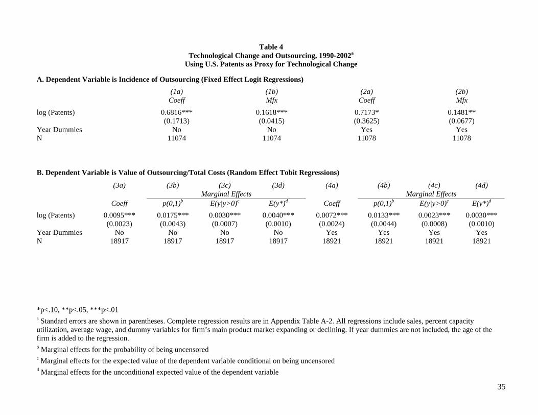
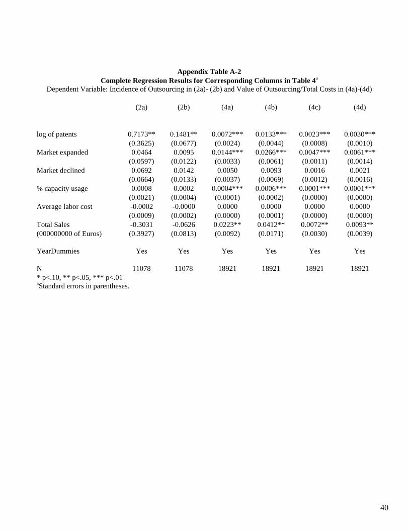
Table 4 presents the results of fixed effect Logit and random effect Tobit regressions that

use the exogenous proxy for expected technological change based on patent counts in the U.S.

The complete regressions are shown in Appendix Table A-2. The patent variable is positive and

significant in all columns of Table 4. This is strong evidence of a causal relationship between

17 In column (1) of Table 7 we report the estimated coefficients of a logit regression without firm fixed effects but with industry dummies.

17

expected technological change and the decision to outsource production as well as the extent of

outsourcing. As explained above, we cannot interpret the magnitudes of the coefficients on

patents in Table 4.

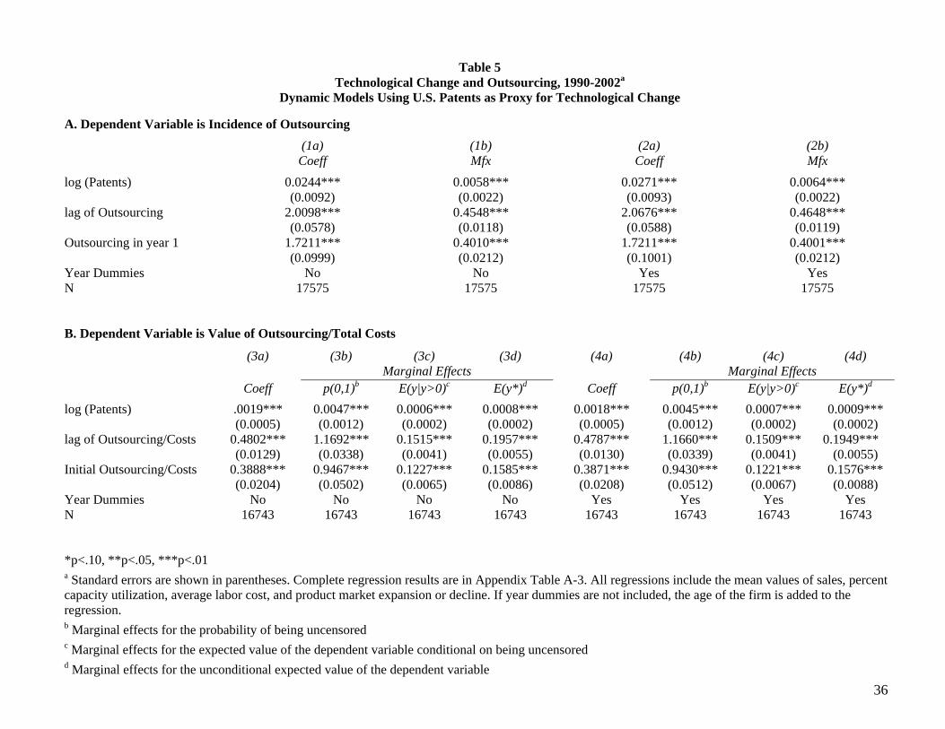
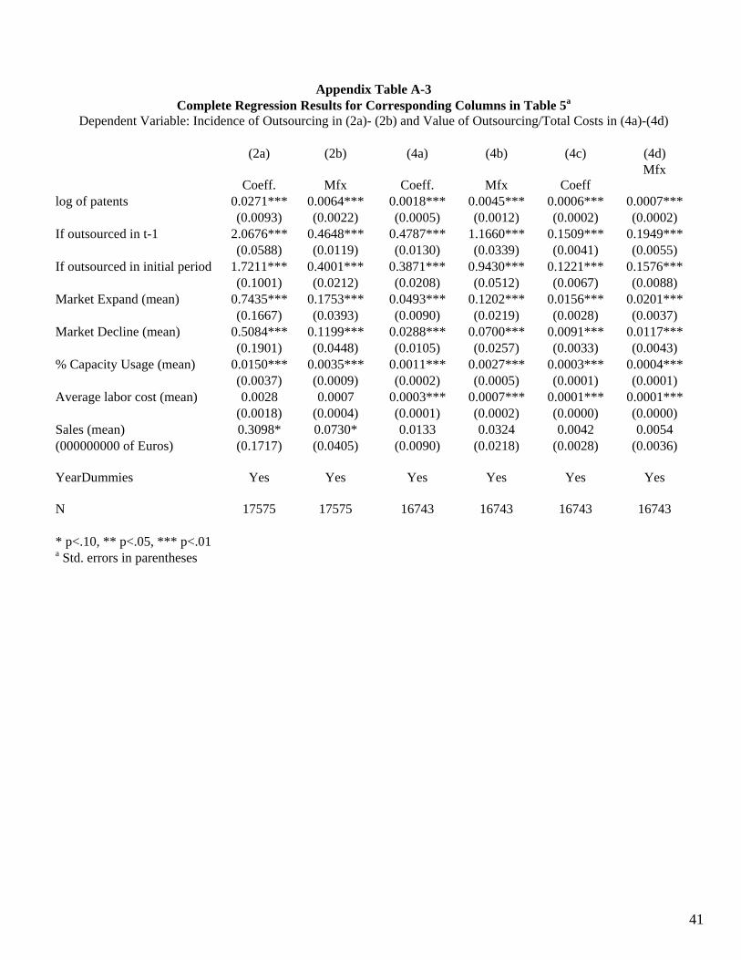
In Table 5, we show the coefficients on the patent variable from random effects Logit and

Tobit regressions that use the specification generated from the model presented in the Appendix;

complete regression results are in Appendix Table A-3. Adding dynamics to the model, i.e.

including lagged outsourcing as a regressor, requires that we address the initial conditions

problem. We follow Wooldridge (2005) in specifying a homoskedastic normal density for the

unobserved firm effect conditional on the exogenous variables and initial outsourcing. We

express the unobserved effect as a linear combination of the time averages of the exogenous

variables, initial outsourcing and a normal error term which is then integrated out from the

likelihood function. The results in Table 5 are virtually identical to those in Table 4; the causal

impact of U.S. patents on the outsourcing decisions of Spanish firms remains even when we add

dynamics to the model.

B. Alternative Explanations

The prior literature on vertical integration and outsourcing has focused on the role played

by relationship-specific investments in a context where at least some part of the contract is non-

verifiable ex post and hence non-contractible ex ante (Gibbons, 2005; Hubbard, 2008; Acemoglu

et.al., 2010). Our model on the other hand, focuses on expectations of technology change and

implicitly assumes full contractibility. It is possible, and perhaps likely, that both approaches - -

expectations about technological change and the existence of incomplete markets - - play a role in

explaining outsourcing. Since we have not controlled for the specificity of investment, we are

concerned that our estimates of the effect of technological expectations may be reflecting the

effect of incomplete markets on outsourcing.

18

In order to control for the effect of incomplete markets on outsourcing, we turn to the

proxy for relationship-specific investments created by Nunn (2007). Nunn used 1997 data to

calculate the proportion of each industry’s intermediate inputs that are sold on an organized

exchange or reference priced in a trade publication. He defines “differentiated inputs” as inputs

that are neither sold on an organized exchange nor reference priced in a trade publication. As in

Nunn (2007), we use the measure of differentiated inputs as a proxy for the extent to which an

industry is subject to industry-specific investments. We matched Nunn’s data to the industrial

sectors in the ESEE and re-estimated the regressions in Table 4 adding the differentiated inputs

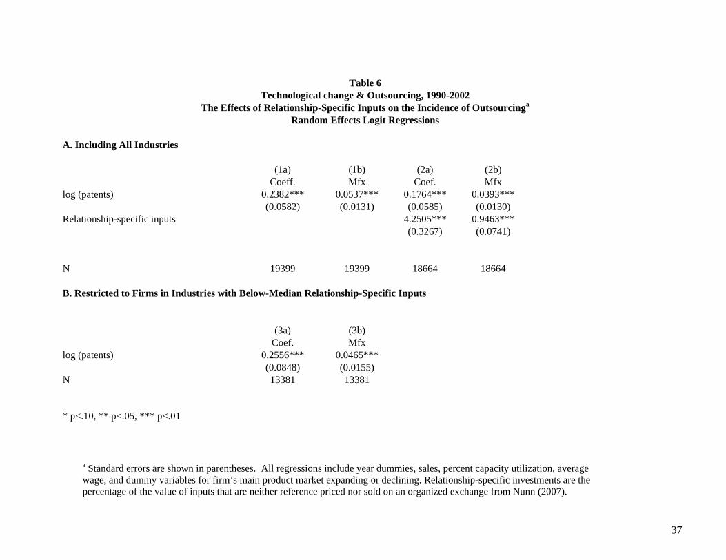
variable. 18 The results, shown in Panel A of Table 6, demonstrate that the patent variable

remains positive and significant. Note also that the effect of the differentiated inputs variable is

positive and significant which is consistent with the property rights theory in the case of the input

supplier’s investments dominating the relationship.19 The positive coefficient on the differentiated

inputs variable rules out a role for the transactions cost theory because this theory predicts that

vertical integration is more likely in the presence of relationship-specific investments.

In Panel B, we delete firms that are in industries that have a large share of relationship-

specific inputs, defined as having a value above the median for the Nunn variable. In this way we

restrict the analysis to firms in industries which have a small share of relationship-specific inputs.

Since the property rights theory of outsourcing is based on the role of relationship-specific inputs,

by focusing on industries where relationship-specific inputs are less important, the property rights

theory of outsourcing would have less relevance for these industries. In Panel B, we find that the

patent variable remains positive and significant for these industries. In other words, our finding

regarding a positive relationship between U.S. patent filings and production outsourcing by

18 We are unable to estimate fixed effects Logit regressions because the Nunn variables are only available for one year. 19 The Nunn variable is positively but marginally significantly correlated with the patent measure we use for 1997 (i.e. the mean over 1994-1996) as well as with the mean number of patents over the 1990-2002 time period (.268 and .243, with significance levels of 9 percent and 13 percent, respectively.)

19

Spanish firms holds for firms that are in industries where relationship-specific inputs are not

important. For these firms, the property rights theory would not be relevant, while our model of

expected technological change still applies. Hence, we conclude that our findings on the effects of

technological expectations on outsourcing do not reflect the effect of incomplete markets.

C. Other Determinants of Outsourcing

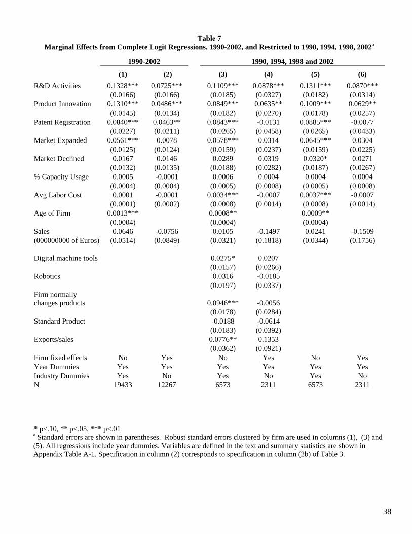
Table 7 presents the coefficients on the non-technology variables described in Section III.

Column (2) corresponds to the specification in column (2b) of Table 3. Column (1) shows the

results without firm fixed effects. In columns (3) through (6), the analysis is restricted to 1990,

1994, 1998 and 2002 because these are the only years in which data on some of the non-

technology variables were collected. Columns (3) and (4) use identical specifications, except that

Column (4) includes firm fixed effects. Finally, Columns (5) and (6) report the specifications

from Columns (1) and (2) but restrict the sample to the four years in which data for all of the non-

technology variables are available.

Unlike the proxies for expected technological change, the coefficients on the non-

technology variables in the model are not robust to the inclusion of fixed effects. When firm fixed

effects are not included in the regressions, some of the non-technology variables are significant,

supporting results from the prior literature. As shown in previous research (Abraham and Taylor,

1996; Holl (2008) the volatility of demand for the product as proxied by market expansion, is

positively correlated with the probability of outsourcing. High average labor costs are also

associated with outsourcing in columns (3) and (5), consistent with previous work (Abraham and

Taylor, 1996). But we find no effect of sales which is at odds with the prediction of our model.20

The firm’s export propensity is positively correlated with outsourcing. But, importantly, none of

these results remain significant when we add fixed effects. We conclude that findings from 20 Holl (2008) suggested that large firms may be more likely to outsource because they have greater capacity to establish and manage subcontracting relationships. If this is true, it would offset the negative relationship that our model predicts.

20

previous studies that rely on cross-sectional analyses may not be robust.

V. Conclusions

Previous research on the relationship between technology and outsourcing has focused on

the roles played by asset specificity, technological diffusion, and information and

communications technology. In this paper we study the outsourcing of production and we propose

an alternative perspective on the relationship between technological change and outsourcing. We

present a dynamic model that shows that outsourcing becomes more beneficial to the firm when

technology is changing rapidly. The intuition behind the model is that as the pace of innovations

in production technology increases, the less time the firm has to amortize the sunk costs

associated with purchasing the new technologies. This makes producing in-house with the latest

technologies relatively more expensive than outsourcing. The model therefore provides an

explanation for the recent increase in outsourcing that has taken place in an environment of

increased expectations for technological change.

We test the predictions of the model using a panel dataset on Spanish firms for the time

period 1990 through 2002. This dataset is superior to those used in previous studies of

outsourcing because it enables us to observe changes within firms over a long time period. Our

econometric analysis controls for unobservable fixed characteristics of the firms and, most

importantly, uses an exogenous measure of expected technological change, i.e. the number of

patents granted by the U.S. patents office in the Spanish firm’s industrial sector. The empirical

results support the main prediction of the model, namely, that all other things equal, outsourcing

of production increases with expected technological change. Our use of the patent variable

enables us to conclude that this relationship is causal; no prior study has been able to provide

causal evidence of the impact of technological change on production outsourcing. We also show

that our results are robust to the inclusion of a measure of relationship-specific investments and

21

furthermore that the patents variable remains significant when the analysis is restricted to

industries with little relationship-specific investments. This shows that our results cannot be

explained by the transactions costs or property rights theories of the firm. Furthermore, while the

existing literature has found evidence that non-technology variables play a role in the decision to

outsource, we find no such evidence here when accounting for firms’ fixed effects.

22

References

Abraham, K. and S. Taylor (1996). “Firms’ Use of Outside Contractors: Theory and Evidence.” Journal of Labor Economics 14: 394-424.

Abramovsky, L. and R. Griffith (2006). “Outsourcing and Offshoring of Business Services: How Important is ICT?” Journal of the European Economic Association 4:594-601.

Acemoglu, D., P. Aghion, R. Griffith, and F. Ziliboti (2010), “Vertical Integration and Technology: Theory and Evidence,” Journal of the European Economic Association.

Amiti, M. and S.J. Wei (2006). “Service Offshoring and Productivity: Evidence from the United States”, NBER Working Paper 11926.

Antras, Pol (2005a). “Property Rights and the International Organization of Production,” AEA Papers and Proceedings, 95(2): 25-32.

Antras, Pol (2005b). “Incomplete Contracts and the Product Cycle.” American Economic Review, 95(4): 1054-73.

Arndt, S.W. and H. Kierzkowski (2001). Fragmentation: New Production Patterns in the World Economy (New York: Oxford University Press).

Autor, D. (2001). “Why Do Temporary Help Firms Provide Free General Skills Training?” Quarterly Journal of Economics, 118 (4): 1409-1448.

Baccara, M. (2007). “Outsourcing, Information Leakage and Consulting Firms,” The Rand Journal of Economics, 38:269-289.

Baker, G. and Hubbard, T. (2003): “Make versus Buy in Trucking: Asset Ownership, Job Design and Information,” American Economic Review, June: 551-572.

Bartel, A., Ichniowski, C. and K. Shaw (2007). “How Does Information Technology Affect Productivity? Plant-Level Comparisons of Product Innovation, Process Improvement and Worker Skills,” Quarterly Journal of Economics, 122(4): 1721-1758.

Benkard, C. Lanier (2000). “Learning and Forgetting: The Dynamics of Aircraft Production,” American Economic Review, September: 1034-54.

Cohen W.M. and D.A. Levinthal (1989). “Innovation and Learning: The Two Faces of R&D”, Economic Journal, September: 569-596.

Diaz-Mora, C. (2005): “Determinants of Outsourcing Production: A Dynamic Panel Data Approach for Manufacturing Industries.” Foundation for Applied Economics Studies working paper.

Feenstra, R.C. and G.H. Hanson (1999). “The Impact of Outsourcing and High-Technology Capital on Wages: Estimates for the United States, 1979-1990”, Quarterly Journal of Economics 114:907-941.

Girma and Gorg (2004). “Outsourcing, Foreign Ownership, and Productivity: Evidence from UK Establishment-level Data,” Review of International Economics 12:817-832.

23

Gibbons, Robert (2005). “Four Formal(izable) Theories of the Firm?” Journal of Economic Behavior & Organization 58:200-245.

Gordon, Robert J. (1990). The Measurement of Durable Goods Prices, Chicago: University of Chicago Press

Gorg, H., A. Hanley and E. Strobl (2007). “Productivity Effects of International Outsourcing: Evidence from Plant-level Data”, Canadian Journal of Economics.

Gorg, H. and A. Hanley (2007). “International Services Outsourcing and Innovation: An Empirical Investigation”. working paper.

Grossman, S. and O. Hart (1986). “The Costs and Benefits of Ownership: A Theory of Vertical and Lateral Integration”, Journal of Political Economy 94(4): 691-719.

Grossman, S. and E. Helpman (2003). “Outsourcing versus FDI in Industry Equilibrium,” Journal of the European Economic Association, 1(2-3): 317-327.

Grossman, S. and E. Helpman (2005). “Outsourcing in a Global Economy.” Review of Economic Studies, 72(1): 135-169. Hall, B. H., A. B. Jaffe, and M. Tratjenberg (2001). "The NBER Patent Citation Data File: Lessons, Insights and Methodological Tools." NBER Working Paper 8498. Holl, A. (2008). “Production Subcontracting and Location,” Regional Science and Urban Economics 38(3): 299-309.

Hubbard, T. (2008). “Viewpoint: Empirical research on firms’ boundaries”, Canadian Journal of Economics 41:341-359.

Johnson, Daniel K.N. (2002), “The OECD Technology Concordance (OTC): Patents by Industry of Manufacture and Sector of Use”.

Lewis, T.R. and D.E.M. Sappington (1991). “Technological Change and the Boundaries of the Firm,” American Economic Review 81: 887-900.

Lileeva, A. and J. Van Biesebroeck (2008). “Outsourcing When Investments are Specific and Complementary.” NBER Working Paper No. 14477, November.

Lopez, A. (2002). “Subcontratacion de servicios y produccion: evidencia par alas empresas manufactureras espanolas,” Econmia Indsutrial, 348:127-140.

Magnani, E (2006). “Technological Diffusion, the Diffusion of Skill and the Growth of Outsourcing in US Manufacturing,” Economics of Innovation and New Technology

Mol, M. (2005). “Does Being R&D-Intensive Still Discourage Outsourcing? Evidence from Dutch Manufacturing,” Research Policy 34:571-582.

Nunn, N. (2007). “Relationship-Specificity, Incomplete Contracts, and the Pattern of Trade,” The Quarterly Journal of Economics, May, 569-600.

Ono, Y. (2007). “Outsourcing Business Services and the Scope of Local Markets,” Regional Science and Urban Economics 37: 220-238.

Williamson, O. (1975). Markets and Hierarchies: Analysis and Antitrust Implications, New

24

York: The Free Press.

Williamson, O. (1985). The Economic Institutions of Capitalism: Firms, Markets, Relational Contracting, New York: The Free Press.

Wooldridge, J. (2002). Econometric Analysis of Cross Section and Panel Data, Cambridge: MIT Press.

Wooldridge, J. (2005). “Simple Solutions to the Initial Conditions Problem for Dynamic, Nonlinear Panel Data Models with Unobserved Heterogeneity,” Journal of Applied Econometrics 20: 39-54.

25

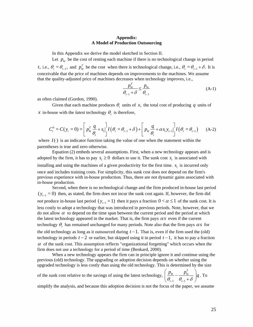
Appendix:

A Model of Production Outsourcing In this Appendix we derive the model sketched in Section II. Let ktp be the cost of renting each machine if there is no technological change in period

,t i.e., 1= ,−t tθ θ and Tktp be the cost when there is technological change, i.e., 1= .− +t tθ θ δ It is

conceivable that the price of machines depends on improvements to the machines. We assume that the quality-adjusted price of machines decreases when technology improves, i.e.,

1 1− −

≤+

Tkt kt

t t

p pθ δ θ

(A-1)

as often claimed (Gordon, 1990). Given that each machine produces tθ units of ,x the total cost of producing q units of

x in-house with the latest technology tθ is therefore,

( ) ( )01 1 1= ( = 0) = = =− − −

⎡ ⎤ ⎡ ⎤+ + + +⎢ ⎥ ⎢ ⎥

⎣ ⎦ ⎣ ⎦T

t t kt t t t kt t t t tt t

q qC C y p s I p s y Iθ θ δ α θ θθ θ

(A-2)

where ( )⋅I is an indicator function taking the value of one when the statement within the parentheses is true and zero otherwise.

Equation (2) embeds several assumptions. First, when a new technology appears and is adopted by the firm, it has to pay 0≥ts dollars to use it. The sunk cost ts is associated with installing and using the machines of a given productivity for the first time. ts is incurred only once and includes training costs. For simplicity, this sunk cost does not depend on the firm's previous experience with in-house production. Thus, there are not dynamic gains associated with in-house production.

Second, when there is no technological change and the firm produced in-house last period 1( = 0)−ty then, as stated, the firm does not incur the sunk cost again. If, however, the firm did

not produce in-house last period 1( = 1)−ty then it pays a fraction 0 < 1≤α of the sunk cost. It is less costly to adopt a technology that was introduced in previous periods. Note, however, that we do not allow α to depend on the time span between the current period and the period at which the latest technology appeared in the market. That is, the firm pays sα even if the current technology tθ has remained unchanged for many periods. Note also that the firm pays sα for the old technology as long as it outsourced during 1.−t That is, even if the firm used the (old) technology in periods 2−t or earlier, but skipped using it in period 1,−t it has to pay a fraction α of the sunk cost. This assumption reflects "organizational forgetting" which occurs when the firm does not use a technology for a period of time (Benkard, 2000).

When a new technology appears the firm can in principle ignore it and continue using the previous (old) technology. The upgrading or adoption decision depends on whether using the upgraded technology is less costly than using the old technology. This is determined by the size

of the sunk cost relative to the savings of using the latest technology, 1 1− −

⎛ ⎞−⎜ ⎟+⎝ ⎠

Tkt kt

t t

p p qθ θ δ

. To

simplify the analysis, and because this adoption decision is not the focus of the paper, we assume

26

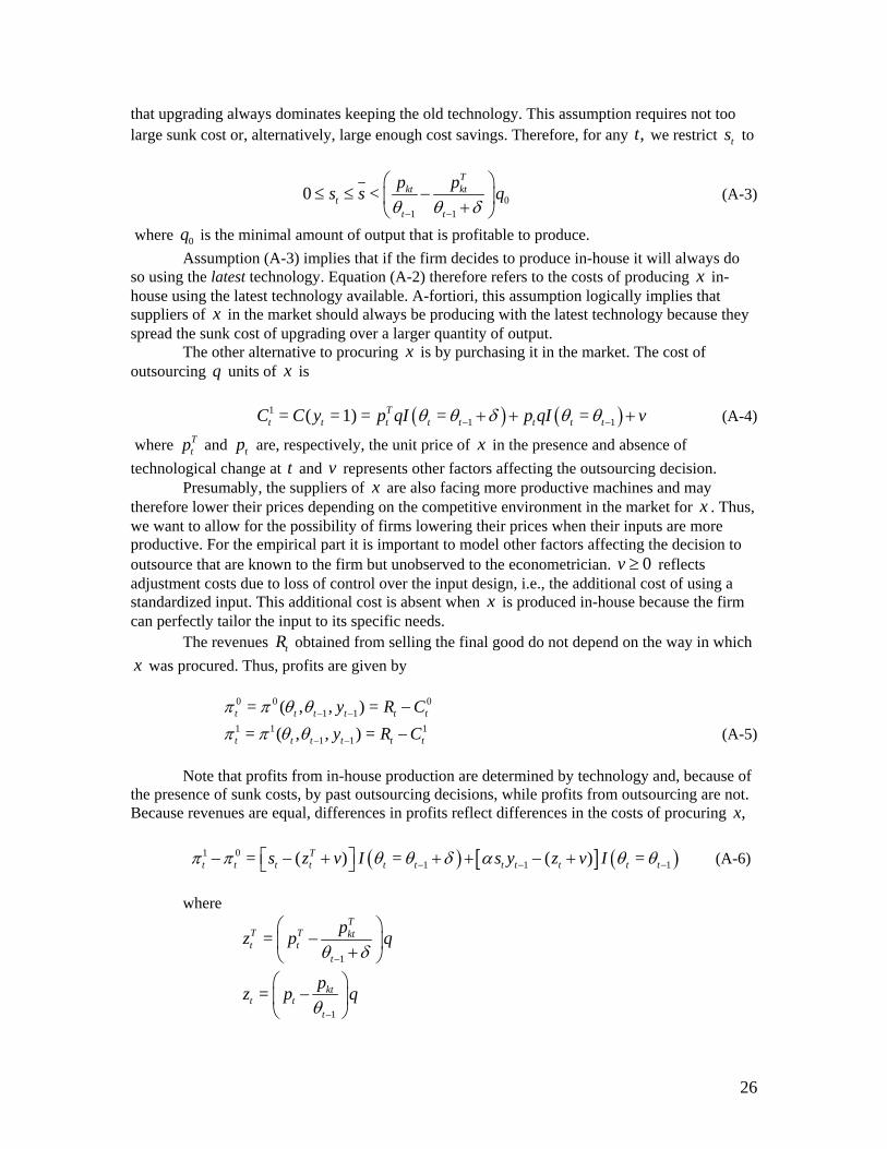
that upgrading always dominates keeping the old technology. This assumption requires not too large sunk cost or, alternatively, large enough cost savings. Therefore, for any ,t we restrict ts to

0

1 1

0 <− −

⎛ ⎞≤ ≤ −⎜ ⎟+⎝ ⎠

Tkt kt

tt t

p ps s qθ θ δ

(A-3)

where 0q is the minimal amount of output that is profitable to produce. Assumption (A-3) implies that if the firm decides to produce in-house it will always do

so using the latest technology. Equation (A-2) therefore refers to the costs of producing x in-house using the latest technology available. A-fortiori, this assumption logically implies that suppliers of x in the market should always be producing with the latest technology because they spread the sunk cost of upgrading over a larger quantity of output.

The other alternative to procuring x is by purchasing it in the market. The cost of outsourcing q units of x is

( ) ( )1

1 1= ( = 1) = = =− −+ + +Tt t t t t t t tC C y p qI p qI vθ θ δ θ θ (A-4)

where Ttp and tp are, respectively, the unit price of x in the presence and absence of

technological change at t and v represents other factors affecting the outsourcing decision. Presumably, the suppliers of x are also facing more productive machines and may

therefore lower their prices depending on the competitive environment in the market for x . Thus, we want to allow for the possibility of firms lowering their prices when their inputs are more productive. For the empirical part it is important to model other factors affecting the decision to outsource that are known to the firm but unobserved to the econometrician. 0≥v reflects adjustment costs due to loss of control over the input design, i.e., the additional cost of using a standardized input. This additional cost is absent when x is produced in-house because the firm can perfectly tailor the input to its specific needs.

The revenues tR obtained from selling the final good do not depend on the way in which x was procured. Thus, profits are given by

0 0 0

1 1= ( , , ) =− − −t t t t t ty R Cπ π θ θ

1 1 11 1= ( , , ) =− − −t t t t t ty R Cπ π θ θ (A-5)

Note that profits from in-house production are determined by technology and, because of

the presence of sunk costs, by past outsourcing decisions, while profits from outsourcing are not. Because revenues are equal, differences in profits reflect differences in the costs of procuring ,x

( ) [ ] ( )1 0

1 1 1= ( ) = ( ) =− − −⎡ ⎤− − + + + − +⎣ ⎦T

t t t t t t t t t t ts z v I s y z v Iπ π θ θ δ α θ θ (A-6)

where

1

=−

⎛ ⎞−⎜ ⎟+⎝ ⎠

TT T ktt t

t

pz p qθ δ

1

=−

⎛ ⎞−⎜ ⎟

⎝ ⎠kt

t tt

pz p qθ

27

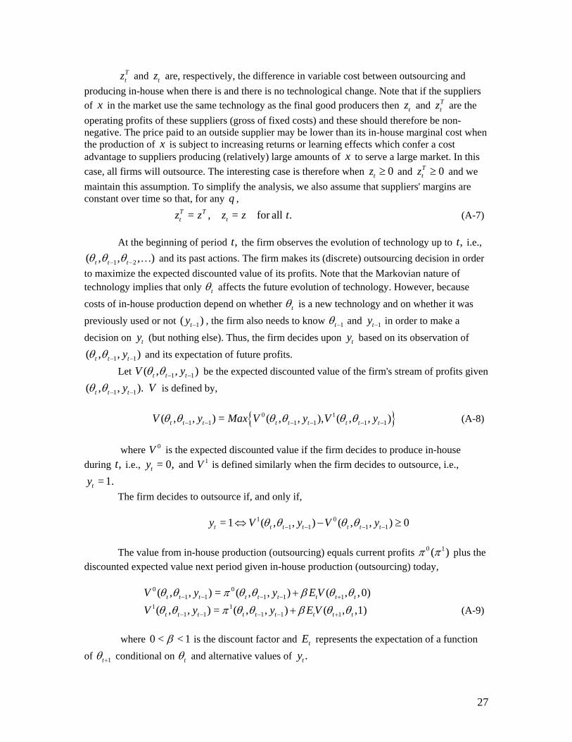
Ttz and tz are, respectively, the difference in variable cost between outsourcing and

producing in-house when there is and there is no technological change. Note that if the suppliers of x in the market use the same technology as the final good producers then tz and T

tz are the operating profits of these suppliers (gross of fixed costs) and these should therefore be non-negative. The price paid to an outside supplier may be lower than its in-house marginal cost when the production of x is subject to increasing returns or learning effects which confer a cost advantage to suppliers producing (relatively) large amounts of x to serve a large market. In this case, all firms will outsource. The interesting case is therefore when 0≥tz and 0≥T

tz and we maintain this assumption. To simplify the analysis, we also assume that suppliers' margins are constant over time so that, for any q ,

= , = for all .T Tt tz z z z t (A-7)

At the beginning of period ,t the firm observes the evolution of technology up to ,t i.e.,

1 2( , , , )− − Kt t tθ θ θ and its past actions. The firm makes its (discrete) outsourcing decision in order to maximize the expected discounted value of its profits. Note that the Markovian nature of technology implies that only tθ affects the future evolution of technology. However, because costs of in-house production depend on whether tθ is a new technology and on whether it was previously used or not 1( )−ty , the firm also needs to know 1−tθ and 1−ty in order to make a decision on ty (but nothing else). Thus, the firm decides upon ty based on its observation of

1 1( , , )− −t t tyθ θ and its expectation of future profits. Let 1 1( , , )− −t t tV yθ θ be the expected discounted value of the firm's stream of profits given

1 1( , , ).− −t t tyθ θ V is defined by, { }0 1

1 1 1 1 1 1( , , ) = ( , , ), ( , , )− − − − − −t t t t t t t t tV y Max V y V yθ θ θ θ θ θ (A-8)

where 0V is the expected discounted value if the firm decides to produce in-house

during ,t i.e., = 0,ty and 1V is defined similarly when the firm decides to outsource, i.e., = 1.ty

The firm decides to outsource if, and only if, 1 0

1 1 1 1= 1 ( , , ) ( , , ) 0− − − −⇔ − ≥t t t t t t ty V y V yθ θ θ θ

The value from in-house production (outsourcing) equals current profits 0 1( )π π plus the discounted expected value next period given in-house production (outsourcing) today,

0 0

1 1 1 1 1( , , ) = ( , , ) ( , ,0)− − − − ++t t t t t t t t tV y y E Vθ θ π θ θ β θ θ

1 11 1 1 1 1( , , ) = ( , , ) ( , ,1)− − − − ++t t t t t t t t tV y y E Vθ θ π θ θ β θ θ (A-9)

where 0 < < 1β is the discount factor and tE represents the expectation of a function

of 1+tθ conditional on tθ and alternative values of .ty

28

In order to evaluate the last terms in (A-9) we note that because technology in period 1+t remains at tθ with probability (1 )−λ or jumps to +tθ δ with probability λ we have,

1( , ,0) = (1 ) ( , ,0) ( , ,0)+ − + +t t t t t t tE V V Vθ θ λ θ θ λ θ δ θ 1( , ,1) = (1 ) ( , ,1) ( , ,1)+ − + +t t t t t t tE V V Vθ θ λ θ θ λ θ δ θ

Given our simplifying assumptions, when a new technology appears the costs of both

alternatives -- outsourcing and in-house production -- do not depend on 1.−ty Thus, when there is technological change, the past history of in-house production does not matter. This implies,

( , ,0) = ( , ,1).+ +t t t tV Vθ δ θ θ δ θ Given the model's assumptions

0

( , ,1) ( , ,0) = ( ) ( )⎡ ⎤− − − ≡ −⎢ ⎥⎣ ⎦∫s

t t t tV V s G s ds B sθ θ θ θ α α (A-10)

where G is the distribution function of s and

0

( ) = ( ) 0− ≥∫s

B s s G s ds

( )

=1 (1 )

+− −

z vsβ λ α

P roof. Using (A-8) when 1 = =+t tθ θ θ and = 1ty as well as (A-9) we get

{ }0 1 0( , ,1) = ( , ,1) 0, ( , ,1) ( , ,1)+ −V V Max V Vθ θ θ θ θ θ θ θ

[ ]{ }0 1 0= ( , ,1) 0, ( , ,1) ( , ,1) (1 ) ( , ,1) ( , ,0)+ − + − −V Max V Vθ θ π θ θ π θ θ β λ θ θ θ θ

Similarly, we have

[ ]{ }0 1 0( , ,0) = ( , ,0) 0, ( , ,0) ( , ,0) (1 ) ( , ,1) ( , ,0)+ − + − −V V Max V Vθ θ θ θ π θ θ π θ θ β λ θ θ θ θ

The difference in the firm's value between outsourcing and in-house production when 1 = =+t tθ θ θ is therefore

0 0( , ,1) ( , ,0) = ( , ,1) ( , ,0)− −V V V Vθ θ θ θ θ θ θ θ

[ ]{ }1 00, ( , ,1) ( , ,1) (1 ) ( , ,1) ( , ,0)+ − + − −Max V Vπ θ θ π θ θ β λ θ θ θ θ

[ ]{ }1 00, ( , ,0) ( , ,0) (1 ) ( , ,1) ( , ,0)− − + − −Max V Vπ θ θ π θ θ β λ θ θ θ θ

From (A-9) and (A-5) we have 0 0 0 01( , ,1) ( , ,0) = ( , ,1) ( , ,0) = .+− − − tV V sθ θ θ θ π θ θ π θ θ α

Let 1( , ,1) ( , ,0) = +− tV V Dθ θ θ θ and 11= ++

⎛ ⎞−⎜ ⎟

⎝ ⎠kt

tt

pz p qθ

(which is constant over time by

assumption (7)). 1+tD must satisfy,

{ } { }1 1 1 1 1= 0, (1 ) 0, (1 )+ + + + +− + − − + − − − − + −t t t t tD s Max s z v D Max z v Dα α β λ β λ

This implies 1 0.+ ≤tD As explained above we assume that 0≥z and therefore

{ }10, (1 ) = 0.+− − + − tMax z v Dβ λ Thus,

29

{ }1 1 1 1= 0, (1 )+ + + +− + − − + −t t t tD s Max s z v Dα α β λ

For ( )101 (1 )+

+≤ ≤ ≡

− −tz vs s

β λ α we let 1+tD on the RHS be 1,+− tsα and for < ≤s s s we let

the RHS be equal to .1 (1 )

+−

− −z vβ λ

We want to check that the RHS operator returns these

values. It can be easily checked that

{ }1 1

1 1 1 1

1

0= 0, (1 ) =

= <1 (1 )

+ +

+ + + +

+

⎧⎪− ≤ ≤⎪⎪− + − − + − ⎨⎪ +⎪− − ≤

− −⎪⎩

t t

t t t t

t

s s sD s Max s z v D

z v s s s s

αα α β λ

αβ λ

If >s s then 1( , ,1) ( , ,0) = +− −t t t t tV V sθ θ θ θ α for any 1 .+ ≤ts s Note that 1+tD depends on 1+ts and we denote 1 1= ( ).+ +t tD D s We now average 1+tD

over 1+ts using the distribution of sunk costs .G Abusing the notation, we obtain

0

( , ,1) ( , ,0) = ( ) ( )⎡ ⎤− − +⎢ ⎥⎣ ⎦∫ ∫s s

sV V sg s ds sg sθ θ θ θ α

0

= ( )⎡ ⎤− −⎢ ⎥⎣ ⎦∫s

s G s dsα

This proves equation (A-10).

Note that 0

( ) ≤∫sG s ds s and therefore ( , ,1) ( , , 0) 0− ≤V Vθ θ θ θ because, when there is

no technological change, outsourcing at 1+t is more costly that producing in-house (there are no sunk costs since the firm is already using the latest technology at )t .

Using (A-6), (A-10) and the equality between ( , ,0)+t tV θ δ θ and ( , ,1),+t tV θ δ θ the

gains from outsourcing 1 01 1 1 1( , , ) ( , , )− − − −−t t t t t tV y V yθ θ θ θ can be written as,

1

1 0

1 1

(1 ) ( ) ==

(1 ) ( ) =

−

− −

⎧ − − − − +⎪− ⎨⎪ − − − −⎩

Tt t t

t t t t

s z v B sV V

s y z v B s

β λ α θ θ δ

α β λ α θ θ (A-11)

These equations completely determine the firm's outsourcing decision in period t as a

function of the firm's sunk cost at t and ( )1 1, ,− −t t tyθ θ and other factors ( , , ).Tz z v In every

period, the firm draws a sunk cost from the distribution G and decides whether to outsource or not according to (A-11). It is important to have heterogeneity in ts (or in )v . Otherwise, all firms of a given size q would be either outsourcing or producing in-house which is in general contrary to the facts.

The first row in (A-11) indicate that when there is technological change the decision to outsource does not depend on 1−ty . This is a result of our assumption on the lack of dynamic

30

gains from previous in-house experience. Thus, the probability of outsourcing at t conditional on a technological jump is,

( )1( = 1| = , , , ) = (1 ) ( ))− + ≥ + + −T Tt t t tP y z z v P s z v B sθ θ δ β λ α (A-12)

( )= 1 (1 ) ( )− + + −TG z v B sβ λ α

It can be easily shown that

( ) = 1 ( ) 0− ≥

dB s G sd s

( )

= 01 (1 )

∂− ≤

∂ − −s sβλ β λ

( )1 ( )( ) = 01 (1 )−∂

− ≤∂ − −

G s sB s βλ β λ

where g is the density function of .s When technological change occurs, the probability of outsourcing increases with λ and

decreases with .+z v Thus, firms facing higher expectations of technological change in their inputs are more likely to outsource, while larger firms (larger )q and firms facing higher per unit cost of outsourcing are less likely to outsource.

Note that when there is no technological change, 1= ,−t tθ θ and the firm did not outsource in the previous period, 1 = 0,−ty the gains from outsourcing are always non-positive. Because marginal cost of in-house production is lower than tp and the firm already paid the sunk cost (since it was producing in-house last period with the latest technology which did not change) it will continue producing in-house in period .t That is,

1 1( = 1| = 0, = , , , ) = 0− −

Tt t t tP y y z z vθ θ (A-13)

In other words, the model implies that in-house producers will only outsource when there

is technological change. When the firm outsourced in period 1,−t and there is no technological change, it may

decide to produce in-house in period t if the realized sunk cost ts is low enough. Thus, the probability of outsourcing is less than one (even if the technology does not change). From (A-11) we can easily compute,

1 1( = 1| = 1, = , , , ) = ( (1 ) ( ))− −

+≥ + −T

t t t t tz vP y y z z v P s B sθ θ β λα

(A-14)

= 1 (1 ) ( )+⎛ ⎞− + −⎜ ⎟⎝ ⎠

z vG B sβ λα

As in the previous case, the probability of outsourcing conditional on ( )1 1, ,− −t t tyθ θ

increases with λ and decreases with .+z v Thus, when λ increases and new production technologies are more likely to appear in

the future, firms will be more reluctant to buy the current machines today and produce in-house because these technologies will soon be obsolete. Upgrading the technology -- which is the

31

optimal thing to do -- involves incurring a sunk cost di novo. The higher is ,λ the more frequently the new machines arrive and the less time the firm has to amortize the sunk costs. Instead, the firm can use outsourcing to obtain x from supplying firms using the latest technology and avoid the sunk costs. All other things equal, an increase in λ decreases the cost of outsourcing relative to that of in-house production making the firm more likely to decide to outsource. The main prediction of the model that we take to the data is that the probability of outsourcing increases with .λ

32

Mean Std Dev N All If >0FieldFood, beverages 0.210 0.407 3461 0.020 0.100Tobacco products 0.580 0.497 69 0.034 0.068Textile 0.433 0.496 1099 0.048 0.110Wearing apparel 0.536 0.499 1394 0.102 0.190Leather articles 0.391 0.488 744 0.064 0.163Wood products 0.279 0.449 603 0.035 0.127Paper 0.339 0.474 638 0.038 0.115Publishing, printing 0.582 0.493 1136 0.095 0.165Petroleum products, nuclear fuel 0.444 0.527 9 0.081 0.216Basic chemical 0.252 0.435 326 0.017 0.069Paints, varnishes 0.175 0.381 228 0.007 0.041Pharmaceuticals 0.592 0.492 557 0.044 0.076Soaps, detergents, toilet preparation 0.484 0.501 250 0.035 0.075Other chemicals 0.400 0.492 125 0.019 0.048Man-made fibers 0.077 0.277 13 0.001 0.013Rubber and plastics products 0.477 0.500 1066 0.046 0.098Non-metallic mineral products 0.266 0.442 1610 0.027 0.103Basic metals 0.302 0.460 665 0.026 0.089Fabricated metal products 0.477 0.500 1798 0.059 0.125Energy machinery 0.479 0.501 213 0.048 0.105Non-specific purpose machinery 0.715 0.452 281 0.100 0.144Agricultural and forestry machinery 0.775 0.420 89 0.176 0.237Machine-tools 0.712 0.455 104 0.118 0.169Special purpose machinery 0.592 0.492 397 0.100 0.177Weapons and ammunition 0.740 0.443 50 0.125 0.170Domestic appliances 0.622 0.486 196 0.143 0.235Office machinery and computers 0.421 0.497 76 0.035 0.085Electric motors, generators, transformers 0.615 0.489 109 0.053 0.090Electric distribution, control, wire 0.622 0.486 267 0.063 0.098Accumulators, battery 0.646 0.481 79 0.140 0.220Lighting equipment 0.547 0.499 179 0.071 0.135Other electrical equipment 0.727 0.447 176 0.071 0.101Electronic components 0.400 0.491 165 0.023 0.058Signal transmission, telecommunication 0.770 0.422 122 0.084 0.114TV & radio receivers, audiovisual electronics 0.570 0.498 86 0.100 0.182Medical equipment 0.533 0.503 60 0.033 0.066Measuring instruments 0.719 0.451 139 0.108 0.152Industrial process control equipment 0.375 0.518 8 0.007 0.018Optical instruments 0.690 0.467 58 0.120 0.176Motor vehicles 0.539 0.499 951 0.072 0.140Other transport equipment 0.647 0.479 467 0.108 0.171Furniture 0.374 0.484 1077 0.050 0.135Other manufacturing industries 0.530 0.500 560 0.052 0.100

Year1990 0.348 0.476 2045 0.047 0.1381991 0.466 0.499 1879 0.049 0.1161992 0.438 0.496 1797 0.054 0.1271993 0.418 0.493 1698 0.052 0.1301994 0.405 0.491 1683 0.049 0.1221995 0.414 0.493 1519 0.051 0.1251996 0.425 0.494 1539 0.055 0.1321997 0.441 0.497 1741 0.059 0.1351998 0.461 0.499 1608 0.061 0.1321999 0.423 0.494 1594 0.060 0.1442000 0.440 0.497 1719 0.057 0.1302001 0.429 0.495 1580 0.056 0.1332002 0.422 0.494 1567 0.054 0.128

All Firms 0.425 0.494 21700 0.054 0.130

Table 1Value of Outsourcing by Field (1990-2002)

Incidence of Outsourcing Value of Outsourcing ÷ Total Costs

33

1987 1988 1989 1990 1991 1992 1993 1994 1995 1996 1997 1998 1999 2000 2001 2002 TotalFieldFood, beverages 1,678 1,779 1,864 1,864 1,830 1,938 1,967 2,094 2,332 2,232 2,458 2,299 2,335 1,779 643 47 29,139Tobacco products 172 183 180 178 173 161 145 179 201 206 214 216 196 126 37 2 2,569Textile 825 950 966 967 897 957 951 1,064 1,161 1,149 1,245 1,166 1,087 781 323 15 14,504Wearing apparel 337 362 395 417 399 355 409 417 473 488 538 536 529 421 216 7 6,299Leather articles 262 276 275 234 235 214 293 293 328 330 383 349 337 249 98 1 4,157Wood products 346 377 381 396 374 363 387 406 443 444 490 484 468 344 109 5 5,817Paper 918 1,049 1,072 1,113 1,121 1,145 1,176 1,295 1,436 1,383 1,609 1,440 1,356 985 335 13 17,446Publishing, printing 1,143 1,297 1,408 1,474 1,480 1,665 1,671 1,910 2,107 2,277 2,479 2,375 2,154 1,695 528 19 25,682Petroleum products, nuclear fuel 653 652 620 642 670 604 695 660 619 436 135 7 6,393Basic chemical 2,863 3,194 3,438 3,525 3,430 3,445 3,349 3,387 4,112 3,426 3,863 3,440 3,431 2,573 922 49 48,447Paints, varnishes 392 441 477 495 478 488 495 495 588 531 595 520 492 357 123 5 6,972Pharmaceuticals 2,356 2,543 2,736 2,819 2,722 3,125 3,267 3,896 5,276 3,396 4,158 3,694 3,593 2,677 1,124 82 47,464Soaps, detergents, toilet preparation 391 461 450 438 442 443 506 564 697 668 725 645 695 533 226 28 7,912Other chemicals 959 1,051 1,105 1,152 1,143 1,159 1,140 1,187 1,385 1,211 1,362 1,260 1,234 945 353 22 16,668Man-made fibers 257 284 307 286 282 268 278 298 343 332 369 327 331 236 91 2 4,291Rubber and plastics products 2,710 3,164 3,316 3,308 3,324 3,304 3,400 3,561 4,096 3,832 4,268 3,833 3,590 2,496 729 24 48,955Non-metallic mineral products 967 1,069 1,088 1,091 1,112 1,042 1,051 1,094 1,235 1,180 1,369 1,198 1,198 851 250 7 15,802Basic metals 954 1,084 1,037 1,055 1,024 1,027 1,043 1,052 1,105 1,106 1,176 1,174 1,119 914 297 7 15,174Fabricated metal products 1,834 1,996 2,096 2,107 2,095 2,103 2,178 2,279 2,531 2,543 2,883 2,760 2,709 2,103 655 24 32,896Energy machinery 12,403 13,649 14,561 15,040 15,436 15,982 16,217 18,278 20,595 22,171 25,546 24,505 22,241 16,819 6,471 243 260,157Non-specific purpose machinery 12,403 13,649 14,561 15,040 15,436 15,982 16,217 18,278 20,595 22,171 25,546 24,505 22,241 16,819 6,471 243 260,157Agricultural and forestry machinery 12,403 13,649 14,561 15,040 15,436 15,982 16,217 18,278 20,595 22,171 25,546 24,505 22,241 16,819 6,471 243 260,157Machine-tools 12,403 13,649 14,561 15,040 15,436 15,982 16,217 18,278 20,595 22,171 25,546 24,505 22,241 16,819 6,471 243 260,157Special purpose machinery 12,403 13,649 14,561 15,040 15,436 15,982 16,217 18,278 20,595 22,171 25,546 24,505 22,241 16,819 6,471 243 260,157Weapons and ammunition 12,403 13,649 14,561 15,040 15,436 15,982 16,217 18,278 20,595 22,171 25,546 24,505 22,241 16,819 6,471 243 260,157Domestic appliances 12,403 13,649 14,561 15,040 15,436 15,982 16,217 18,278 20,595 22,171 25,546 24,505 22,241 16,819 6,471 243 260,157Office machinery and computers 3,868 4,569 5,037 5,517 5,862 6,495 7,013 8,924 11,600 13,382 16,419 15,714 11,554 6,177 2,391 102 124,624Electric motors, generators, transformers 261 299 326 323 338 335 331 364 407 424 493 474 476 364 124 5 5,344Electric distribution, control, wire 261 299 326 323 338 335 331 364 407 424 493 474 476 364 124 5 5,344Accumulators, battery 261 299 326 323 338 335 331 364 407 424 493 474 476 364 124 5 5,344Lighting equipment 261 299 326 323 338 335 331 364 407 424 493 474 476 364 124 5 5,344Other electrical equipment 261 299 326 323 338 335 331 364 407 424 493 474 476 364 124 5 5,344Electronic components 1,662 2,005 2,221 2,409 2,721 2,887 2,919 3,555 4,311 4,681 5,766 5,847 5,789 4,435 1,968 99 53,275Signal transmission, telecommunication 996 1,163 1,321 1,355 1,466 1,576 1,706 2,195 2,745 3,275 3,969 3,677 2,614 1,454 530 23 30,065TV & radio receivers, audiovisual electronics 1,548 1,803 1,940 2,010 2,130 2,152 2,259 2,857 3,272 3,562 4,153 3,434 2,600 1,492 502 26 35,740Measuring instruments 2,471 2,736 2,972 3,013 3,053 3,122 3,178 3,711 4,130 4,360 5,004 4,775 4,510 3,145 1,016 37 51,233Optical instruments 138 164 180 182 177 171 179 207 236 251 288 266 274 215 72 6 3,006Motor vehicles 4,734 5,074 5,396 5,632 5,342 5,288 5,485 5,806 6,545 6,903 7,633 7,502 7,491 6,727 2,427 83 88,068Other transport equipment 1,150 1,219 1,323 1,328 1,322 1,268 1,321 1,340 1,482 1,518 1,719 1,809 1,679 1,420 561 21 20,480Furniture 1,998 2,180 2,320 2,474 2,424 2,486 2,658 2,916 3,115 3,271 3,656 3,495 3,381 2,702 950 36 40,062Total 126,055 139,511 148,858 153,734 157,453 162,848 166,218 187,390 214,155 225,858 260,773 248,800 225,432 167,821 63,528 2,525 2,650,959

Year

Table 2U.S. Patent Counts Assigned to Spanish Field of Use

34

Table 3 Technological Change and Outsourcing, 1990-2002a

Using Data from Spanish Survey as Proxy for Technological Change

A. Dependent Variable is Incidence of Outsourcing (Fixed Effect Logit Regressions) (1a) (1b) (2a) (2b) Coeff Mfx Coeff Mfx R&D Activities 0.4424*** 0.0971*** 0.3354*** 0.0725*** (0.0829) (0.0187) (0.0780) (0.0166) Product Innovation 0.2715*** 0.0594*** 0.2259*** 0.0486*** (0.0645 (0.0146) (0.0619) (0.0134) Patent Registration 0.1982* 0.0430* 0.2187** 0.0463** (0.1065) (0.0226) (0.1028) (0.0211) Year Dummies No No Yes Yes N 11062 11062 12267 12267 B. Dependent Variable is Value of Outsourcing/Total Costs (Random Effect Tobit Regressions)

(3a) (3b) (3c) (3d) (4a) (4b) (4c) (4d) Marginal Effects Marginal Effects Coeff p(0,1)b E(y|y>0)c E(y*)d Coeff p(0,1)b E(y|y>0)c E(y*)d R&D Activities 0.0312*** 0.0582*** 0.0101*** 0.0132*** 0.0316*** 0.0590*** 0.0102*** 0.0134*** (0.0040) (0.0076) (0.0013) (0.0018) (0.0041) (0.0076) (0.0013) (0.0018) Product Innovation 0.0160*** 0.0297*** 0.0052*** 0.0067*** 0.0145*** 0.0270*** 0.0047*** 0.0061*** (0.0035) (0.0065) (0.0011) (0.0015) (0.0035) (0.0066) (0.0011) (0.0015) Patent Registration 0.0138** 0.0258** 0.0045** 0.0059** 0.0155*** 0.0290*** 0.0050*** 0.0066*** (0.0056) (0.0105) (0.0018) (0.0024) (0.0056) (0.0105) (0.0019) (0.0025) Year Dummies No No No No Yes Yes Yes Yes N 18981 18981 18981 18981 18981 18981 18981 18981 *p<.10, **p<.05, ***p<.01 a Standard errors are shown in parentheses. The full regression for column (2b) appears in column (2) of Table 7. All regressions include sales, percent capacity utilization, average wage, and dummy variables for firm’s main product market expanding or declining. If year dummies are not included, the age of the firm is added to the regression. b Marginal effects for the probability of being uncensored c Marginal effects for the expected value of the dependent variable conditional on being uncensored d Marginal effects for the unconditional expected value of the dependent variable

35

Table 4

Technological Change and Outsourcing, 1990-2002a Using U.S. Patents as Proxy for Technological Change

A. Dependent Variable is Incidence of Outsourcing (Fixed Effect Logit Regressions) (1a) (1b) (2a) (2b) Coeff Mfx Coeff Mfx log (Patents) 0.6816*** 0.1618*** 0.7173* 0.1481** (0.1713) (0.0415) (0.3625) (0.0677) Year Dummies No No Yes Yes N 11074 11074 11078 11078 B. Dependent Variable is Value of Outsourcing/Total Costs (Random Effect Tobit Regressions)

(3a) (3b) (3c) (3d) (4a) (4b) (4c) (4d) Marginal Effects Marginal Effects Coeff p(0,1)b E(y|y>0)c E(y*)d Coeff p(0,1)b E(y|y>0)c E(y*)d log (Patents) 0.0095*** 0.0175*** 0.0030*** 0.0040*** 0.0072*** 0.0133*** 0.0023*** 0.0030*** (0.0023) (0.0043) (0.0007) (0.0010) (0.0024) (0.0044) (0.0008) (0.0010) Year Dummies No No No No Yes Yes Yes Yes N 18917 18917 18917 18917 18921 18921 18921 18921 *p<.10, **p<.05, ***p<.01 a Standard errors are shown in parentheses. Complete regression results are in Appendix Table A-2. All regressions include sales, percent capacity utilization, average wage, and dummy variables for firm’s main product market expanding or declining. If year dummies are not included, the age of the firm is added to the regression. b Marginal effects for the probability of being uncensored c Marginal effects for the expected value of the dependent variable conditional on being uncensored d Marginal effects for the unconditional expected value of the dependent variable

36

Table 5 Technological Change and Outsourcing, 1990-2002a

Dynamic Models Using U.S. Patents as Proxy for Technological Change

A. Dependent Variable is Incidence of Outsourcing (1a) (1b) (2a) (2b) Coeff Mfx Coeff Mfx log (Patents) 0.0244*** 0.0058*** 0.0271*** 0.0064*** (0.0092) (0.0022) (0.0093) (0.0022) lag of Outsourcing 2.0098*** 0.4548*** 2.0676*** 0.4648*** (0.0578) (0.0118) (0.0588) (0.0119) Outsourcing in year 1 1.7211*** 0.4010*** 1.7211*** 0.4001*** (0.0999) (0.0212) (0.1001) (0.0212) Year Dummies No No Yes Yes N 17575 17575 17575 17575 B. Dependent Variable is Value of Outsourcing/Total Costs

(3a) (3b) (3c) (3d) (4a) (4b) (4c) (4d) Marginal Effects Marginal Effects Coeff p(0,1)b E(y|y>0)c E(y*)d Coeff p(0,1)b E(y|y>0)c E(y*)d log (Patents) .0019*** 0.0047*** 0.0006*** 0.0008*** 0.0018*** 0.0045*** 0.0007*** 0.0009*** (0.0005) (0.0012) (0.0002) (0.0002) (0.0005) (0.0012) (0.0002) (0.0002) lag of Outsourcing/Costs 0.4802*** 1.1692*** 0.1515*** 0.1957*** 0.4787*** 1.1660*** 0.1509*** 0.1949*** (0.0129) (0.0338) (0.0041) (0.0055) (0.0130) (0.0339) (0.0041) (0.0055) Initial Outsourcing/Costs 0.3888*** 0.9467*** 0.1227*** 0.1585*** 0.3871*** 0.9430*** 0.1221*** 0.1576*** (0.0204) (0.0502) (0.0065) (0.0086) (0.0208) (0.0512) (0.0067) (0.0088) Year Dummies No No No No Yes Yes Yes Yes N 16743 16743 16743 16743 16743 16743 16743 16743 *p<.10, **p<.05, ***p<.01 a Standard errors are shown in parentheses. Complete regression results are in Appendix Table A-3. All regressions include the mean values of sales, percent capacity utilization, average labor cost, and product market expansion or decline. If year dummies are not included, the age of the firm is added to the regression. b Marginal effects for the probability of being uncensored c Marginal effects for the expected value of the dependent variable conditional on being uncensored d Marginal effects for the unconditional expected value of the dependent variable

37

Table 6 Technological change & Outsourcing, 1990-2002

The Effects of Relationship-Specific Inputs on the Incidence of Outsourcinga

Random Effects Logit Regressions

A. Including All Industries (1a) (1b) (2a) (2b) Coeff. Mfx Coef. Mfx log (patents) 0.2382*** 0.0537*** 0.1764*** 0.0393*** (0.0582) (0.0131) (0.0585) (0.0130) Relationship-specific inputs 4.2505*** 0.9463*** (0.3267) (0.0741) N 19399 19399 18664 18664 B. Restricted to Firms in Industries with Below-Median Relationship-Specific Inputs (3a) (3b) Coef. Mfx log (patents) 0.2556*** 0.0465*** (0.0848) (0.0155) N 13381 13381 * p<.10, ** p<.05, *** p<.01

a Standard errors are shown in parentheses. All regressions include year dummies, sales, percent capacity utilization, average wage, and dummy variables for firm’s main product market expanding or declining. Relationship-specific investments are the percentage of the value of inputs that are neither reference priced nor sold on an organized exchange from Nunn (2007).

38

Table 7 Marginal Effects from Complete Logit Regressions, 1990-2002, and Restricted to 1990, 1994, 1998, 2002a

1990-2002

1990, 1994, 1998 and 2002

(1) (2) (3) (4) (5) (6) R&D Activities 0.1328*** 0.0725*** 0.1109*** 0.0878*** 0.1311*** 0.0870*** (0.0166) (0.0166) (0.0185) (0.0327) (0.0182) (0.0314) Product Innovation 0.1310*** 0.0486*** 0.0849*** 0.0635** 0.1009*** 0.0629** (0.0145) (0.0134) (0.0182) (0.0270) (0.0178) (0.0257) Patent Registration 0.0840*** 0.0463** 0.0843*** -0.0131 0.0885*** -0.0077 (0.0227) (0.0211) (0.0265) (0.0458) (0.0265) (0.0433) Market Expanded 0.0561*** 0.0078 0.0578*** 0.0314 0.0645*** 0.0304 (0.0125) (0.0124) (0.0159) (0.0237) (0.0159) (0.0225) Market Declined 0.0167 0.0146 0.0289 0.0319 0.0320* 0.0271 (0.0132) (0.0135) (0.0188) (0.0282) (0.0187) (0.0267) % Capacity Usage 0.0005 -0.0001 0.0006 0.0004 0.0004 0.0004 (0.0004) (0.0004) (0.0005) (0.0008) (0.0005) (0.0008) Avg Labor Cost 0.0001 -0.0001 0.0034*** -0.0007 0.0037*** -0.0007 (0.0001) (0.0002) (0.0008) (0.0014) (0.0008) (0.0014) Age of Firm 0.0013*** 0.0008** 0.0009** (0.0004) (0.0004) (0.0004) Sales 0.0646 -0.0756 0.0105 -0.1497 0.0241 -0.1509 (000000000 of Euros) (0.0514) (0.0849) (0.0321) (0.1818) (0.0344) (0.1756) Digital machine tools

0.0275* 0.0207

(0.0157) (0.0266) Robotics 0.0316 -0.0185 (0.0197) (0.0337) Firm normally changes products

0.0946*** -0.0056

(0.0178) (0.0284) Standard Product -0.0188 -0.0614 (0.0183) (0.0392) Exports/sales 0.0776** 0.1353 (0.0362) (0.0921) Firm fixed effects No Yes No Yes No Yes Year Dummies Yes Yes Yes Yes Yes Yes Industry Dummies Yes No Yes No Yes No N 19433 12267 6573 2311 6573 2311 * p<.10, ** p<.05, *** p<.01 a Standard errors are shown in parentheses. Robust standard errors clustered by firm are used in columns (1), (3) and (5). All regressions include year dummies. Variables are defined in the text and summary statistics are shown in Appendix Table A-1. Specification in column (2) corresponds to specification in column (2b) of Table 3.

39

Appendix Table A-1 Summary Statistics

Variable Mean Std. Dev. Engaged in R&D activities 0.3748 0.4841 Firm normally changes product 0.2375 0.4256 Engaged in product innovation 0.2475 0.4316 Registered patents 0.0838 0.2771 Product is standardized 0.6292 0.4830 Market expanded 0.3396 0.4736 Market declined 0.1909 0.3931 Uses computer digital machine tools 0.4056 0.4910 Uses robotics 0.2181 0.4130 Average labor cost per employee (thousands of Euros) 25.960 12.222 Export value divided by sales 0.1640 0.2456 Age of firm 23.9305 22.536 Capacity utilization rate 81.8359 15.2313 Total Sales in 2002 (thousands of) Euros 47,200 195,700

40

Appendix Table A-2 Complete Regression Results for Corresponding Columns in Table 4a

Dependent Variable: Incidence of Outsourcing in (2a)- (2b) and Value of Outsourcing/Total Costs in (4a)-(4d) (2a) (2b) (4a) (4b) (4c) (4d) log of patents 0.7173** 0.1481** 0.0072*** 0.0133*** 0.0023*** 0.0030*** (0.3625) (0.0677) (0.0024) (0.0044) (0.0008) (0.0010) Market expanded 0.0464 0.0095 0.0144*** 0.0266*** 0.0047*** 0.0061*** (0.0597) (0.0122) (0.0033) (0.0061) (0.0011) (0.0014) Market declined 0.0692 0.0142 0.0050 0.0093 0.0016 0.0021 (0.0664) (0.0133) (0.0037) (0.0069) (0.0012) (0.0016) % capacity usage 0.0008 0.0002 0.0004*** 0.0006*** 0.0001*** 0.0001*** (0.0021) (0.0004) (0.0001) (0.0002) (0.0000) (0.0000) Average labor cost -0.0002 -0.0000 0.0000 0.0000 0.0000 0.0000 (0.0009) (0.0002) (0.0000) (0.0001) (0.0000) (0.0000) Total Sales -0.3031 -0.0626 0.0223** 0.0412** 0.0072** 0.0093** (000000000 of Euros) (0.3927) (0.0813) (0.0092) (0.0171) (0.0030) (0.0039) YearDummies Yes Yes Yes Yes Yes Yes N 11078 11078 18921 18921 18921 18921 * p<.10, ** p<.05, *** p<.01 aStandard errors in parentheses.

41

Appendix Table A-3

Complete Regression Results for Corresponding Columns in Table 5a Dependent Variable: Incidence of Outsourcing in (2a)- (2b) and Value of Outsourcing/Total Costs in (4a)-(4d)

(2a) (2b) (4a) (4b) (4c) (4d)

Coeff. Mfx Coeff. Mfx Coeff Mfx

log of patents 0.0271*** 0.0064*** 0.0018*** 0.0045*** 0.0006*** 0.0007*** (0.0093) (0.0022) (0.0005) (0.0012) (0.0002) (0.0002) If outsourced in t-1 2.0676*** 0.4648*** 0.4787*** 1.1660*** 0.1509*** 0.1949*** (0.0588) (0.0119) (0.0130) (0.0339) (0.0041) (0.0055) If outsourced in initial period 1.7211*** 0.4001*** 0.3871*** 0.9430*** 0.1221*** 0.1576*** (0.1001) (0.0212) (0.0208) (0.0512) (0.0067) (0.0088) Market Expand (mean) 0.7435*** 0.1753*** 0.0493*** 0.1202*** 0.0156*** 0.0201*** (0.1667) (0.0393) (0.0090) (0.0219) (0.0028) (0.0037) Market Decline (mean) 0.5084*** 0.1199*** 0.0288*** 0.0700*** 0.0091*** 0.0117*** (0.1901) (0.0448) (0.0105) (0.0257) (0.0033) (0.0043) % Capacity Usage (mean) 0.0150*** 0.0035*** 0.0011*** 0.0027*** 0.0003*** 0.0004*** (0.0037) (0.0009) (0.0002) (0.0005) (0.0001) (0.0001) Average labor cost (mean) 0.0028 0.0007 0.0003*** 0.0007*** 0.0001*** 0.0001*** (0.0018) (0.0004) (0.0001) (0.0002) (0.0000) (0.0000) Sales (mean) 0.3098* 0.0730* 0.0133 0.0324 0.0042 0.0054 (000000000 of Euros) (0.1717) (0.0405) (0.0090) (0.0218) (0.0028) (0.0036) YearDummies Yes Yes Yes Yes Yes Yes N 17575 17575 16743 16743 16743 16743 * p<.10, ** p<.05, *** p<.01 a Std. errors in parentheses