Over-Extraction in the Shallow and the Deep { The...1 Over-Extraction in the Shallow and the Deep {...

WATER RESOURCES RESEARCH, VOL. ???, XXXX, DOI:10.1029/,

Over-Extraction in the Shallow and the Deep – The1

Sustainability and Reliability of India’s Groundwater2

Irrigation3

Ram Fishman,1

Tobias Siegfried,1

Pradeep Raj,2

Vijay Modi,3

and Upmanu

Lall1

1Columbia Water Center, The Earth

Institute, Columbia University, New York,

NYC, USA

2Groundwater Department, Government

of Andhra Pradesh, Hyderabad, India

3Department of Mechanical Engineering,

Columbia University, New York, NY, USA

D R A F T March 2, 2011, 11:49am D R A F T

X - 2 FISHMAN ET AL.: EXCESSIVE EXTRACTION IN THE SHALLOW AND THE DEEP

Abstract. The excessive exploitation of aquifers is emerging as a world-4

wide problem, but it is nowhere as dramatic and consequential as it is in In-5

dia, the world’s largest groundwater consumer for irrigation. While the prob-6

lem is usually framed in terms of long-term depletion of fossil aquifers, we7

focus here on the agricultural implications of over-exploitation in aquifer of8

limited storage, such as those that underlie most of peninsular India, by con-9

trasting water table and irrigation dynamics in two irrigation intensive re-10

gions of India that differ in underlying hydrogeology. In the deep alluvial aquifers11

of Punjab of north-western India, water table dynamics are dominated by12

declining trends, while in the hard rock, shallow aquifer region of Telangana13

in southern-central India, dynamics are dominated by short-term fluctua-14

tions. We show that irrigation from the deep aquifers in Punjab is largely15

unaffected by fluctuations in water tables and rainfall, but in the hard rock16

shallow aquifers of Telangana, irrigation is more variable and sensitive to these17

stochastic variables. These findings indicate that energy and land are the bind-18

ing constraints to irrigation in Punjab, but physical water scarcity is the bind-19

ing constraint in Telangana. We argue that over-exploitation of a deep aquifer20

is primarily an issue of long-term sustainability, whereas in a shallow aquifer,21

it leads to increased short-term variability in irrigation and a loss of buffer-22

ing capacity which can be harmful economically.23


FISHMAN ET AL.: EXCESSIVE EXTRACTION IN THE SHALLOW AND THE DEEP X - 3

1. Introduction

The excessive exploitation of groundwater aquifers is emerging as a worldwide problem,24

but it is nowhere as dramatic and consequential as it is in India, the world’s largest con-25

sumer of groundwater (250 km3 per year), and a country where up to 70 % of agricultural26

production and 50 % of the population depend on this vital resource [The World Bank27

and Government of India, 1980; Shah, 2008]. An understanding of the consequences of28

excessive exploitation for agricultural production is clearly an important research agenda.29

However, despite the pervasive indications of excessive extraction around the country,30

documentation or analysis of the associated impacts on irrigated agriculture are hard to31

find. This paper takes a first step in this direction.32

Usually, the problem is posed in terms of consistent declines in water table and the33

implications for the long-term sustainability of irrigated agriculture [Moench, 1992; Rodell34

et al., 2009; Tiwari et al., 2009; Wada et al., 2010]. Such a decline is typical in over-35

exploited aquifers of large storage, such as the alluvial aquifers that cover much of northern36

and western India. In this kind of environment, increases in the use of energy for pumping37

can make up for the decline in water tables while guaranteeing constant or increasing water38

use at the same time. This could be one of the reasons for the difficulty of observing the39

impacts of groundwater depletion on irrigated agriculture, especially in light of the fact40

that in much of India, energy use for pumping is determined by political, rather than41

economic rationale: farmers usually face a flat, low (if any) charge on electricity use for42

pumping, and use as much of it as they can, even while lobbying for increases in its supply.43

144



In India, however, intensive groundwater irrigated agriculture is practiced over a large45

range of hydrogeological conditions. Much of India, in particular, overlays hard rock,46

shallow aquifers of more limited storage. The exploitation of these aquifers has proven47

to be as economically important as that of alluvial aquifers. It has resulted in a similar48

boom in irrigation and agriculture [Shah, 2008], as well as a similar pattern of unregulated49

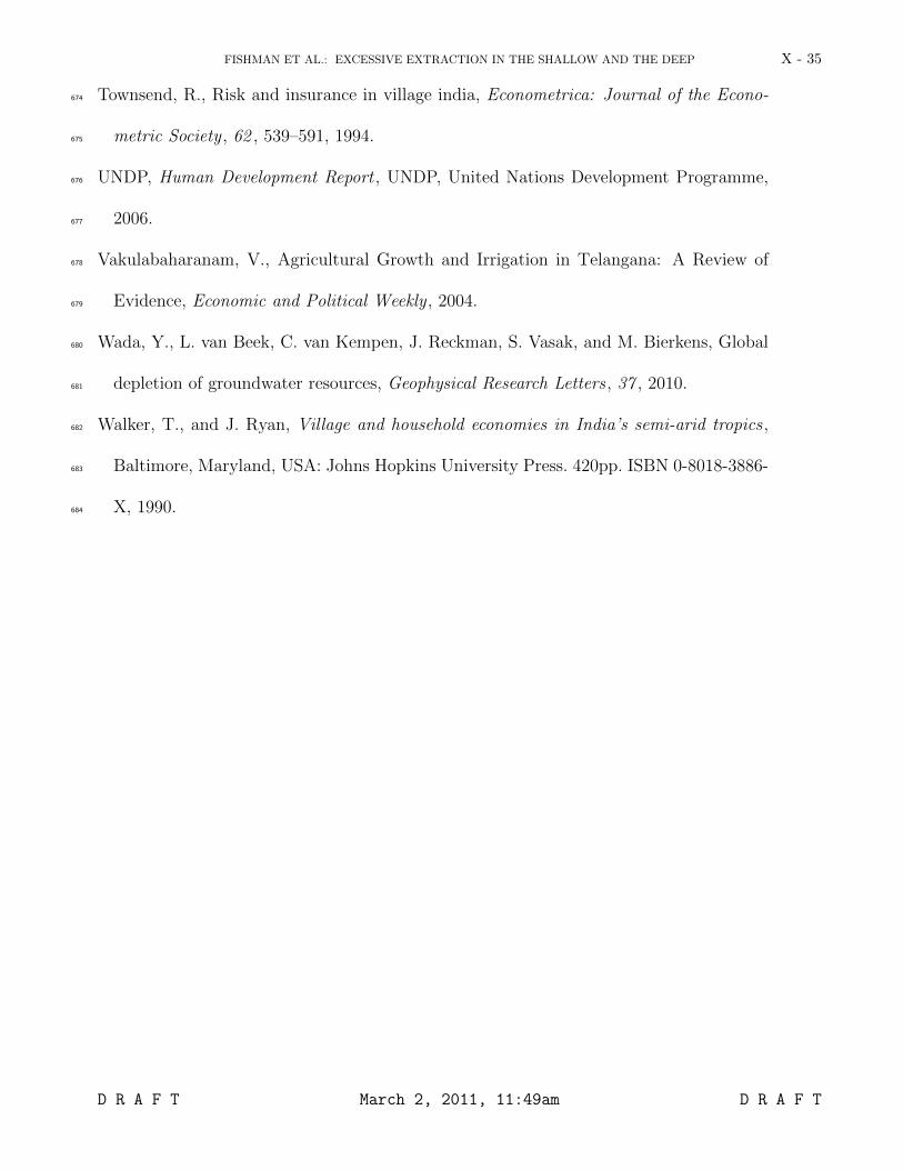
and excessive extraction (Figure 1). In this paper, however, we argue that the nature,50

dynamics and implications of over-exploitation of these shallower aquifers is fundamentally51

different than it is in deep, thick aquifers.52

Our analysis utilizes data on water tables, rainfall and irrigation over the last two53

decades to perform a comparative analysis of coupled groundwater and agricultural dy-54

namics in two key regional hotspots of depletion. These represent the two prominent55

hydrogeological regimes in the country, i.e. the state of Punjab on the one hand [Kumar56

et al., 2007], which overlies the deep alluvial aquifers of the Gangetic basin, and Telangana57

[Raj , 2004a, 2006], in the state of Andhra Pradesh on the other, which overlies shallow,58

fractured hard rock aquifers much like those that cover much of peninsular India.59

While the two regions have similar agricultural energy economies, and both are labeled60

as over-exploited by India’s central groundwater board (see Central Ground Water Board61

[2007], also Figure 1), we find clear differences in their groundwater usage dynamics that62

are consistent with the appearance of bottom effects in the shallow aquifers of Telangana63

and their absence, so far, in the deep aquifers of Punjab. There, the dynamics of both64

water tables and irrigation are dominated by steady secular declines. Conversely, in Telan-65

gana they are dominated by short-term variability (with large welfare costs). In Punjab,66

water supply for irrigation is insensitive to rainfall or water tables, but in Telangana, it67



is highly dependent on both. Thus, groundwater access can make up for a bad rainfall in68

Telangana, but only if the water tables are not excessively low under which the buffering69

ability groundwater is limited. In Punjab, land availability and electricity supply are the70

limiting factors on irrigation but in Telangana, it is water availability.71

Our comparative analysis is intended to highlight unique elements of over-extraction72

of shallower aquifers that tend to receive much less attention in both the policy and73

theoretical literature than the steady declines in water tables in aquifers like Punjab’s.74

We believe such an analysis is important for two reasons. First, it is important in itself75

because, as stated above, shallow, hard rock aquifers support significant parts of India’s76

groundwater irrigated areas and are important sources of water supply all over the world77

[Shiklomanov , 2000; UNDP , 2006]. Second, it can provide an indication of where deeper78

aquifers might be heading in the longer run as water levels approach the bottom, and can79

thus inform the policy debate surrounding groundwater depletion.80

Indeed, while increases in the energy supply allow agriculture and farmers to temporar-81

ily escape the impacts of falling water tables, this process cannot continue indefinitely.82

Eventually, the bottom is reached: either the resource is literally depleted (i.e. the bottom83

of the aquifer reached) or the costs of further deepening wells become prohibitive. When84

that happens, water extraction will have to decline to renewable levels, i.e. to the level85

of natural recharge, and increases in energy use will be of no avail (and we shall argue,86

actually harmful). The time it would take to reach the bottom, however, depends on the87

properties of the aquifer in question, and in particular, on its storage capacity (or the88

depth of its bottom). Where aquifers have a large storage and thus are thick, the impacts89

of falling water tables might still be hidden in agricultural energy usage (for which reliable90



data are very difficult to find) but by looking at low storage, i.e. thinner aquifers, we91

might expect to find more direct evidence of the impacts.92

One insight from our analysis is that while in deep aquifers excessive exploitation (i.e.93

excessive energy usage) is an issue of long-term sustainability, in shallower aquifers it is94

primarily an issue of short-term reliability in water supply. Water tables simply cannot95

decline consistently because they can reach the bottom and can be recovered by abundant96

rains, but they tend to be more variable for these very same reasons. This variability97

translates to lack or reliability in water supply and the associated welfare and economic98

costs. Thus, the classification of a thin aquifer as over-exploited on the basis of short-term99

(annual deficit) data has to be interpreted with caution. Shallow aquifers cannot be over-100

exploited, in terms of a mass deficit, consistently over long periods of time. This is perhaps101

part of the reason they are not detected by the recent satellite gravity measurement based102

methods employed by [Rodell et al., 2009] and [Tiwari et al., 2009], among others, to103

dramatically confirm the extent of depletion over northern India. However, they can be104

over-exploited in years when they are relatively well recharged, and this has the social105

costs we highlight in this paper.106

A second, related, insight has to do with the notion of the buffering service offered107

by groundwater storage against inter-annual fluctuations in rainfall, a major economic108

concern in the semi-arid tropics especially, and in developing countries in particular [Ribot109

et al., 1996]. In shallow aquifers, the initial development of irrigation can provide such110

a buffer, but if excessively developed, can also undermine it. In other words, the inter-111

annual buffer value of groundwater aquifers has a non-monotonic relationship to irrigation112

development. Asymptotically, we will argue it can be completely lost. We will discuss113



how the degree of social aversion to fluctuations in agricultural productions can determine114

the optimal level of irrigation development (in particular, energy usage) and why it may115

be difficult, from the policy perspective, to achieve this optimal level.116

The rest of the paper is organized as follows. In Section 2 we describe the regions117

of study and the data. Section 3 introduces a simple coupled human-natural modeling118

framework of groundwater use and conducts a comparative analysis of the dynamics of119

water tables in the two regions. Section 4 contains a comparative analysis of the dynamics120

of water supply for irrigation. Section 5 discusses the social welfare and policy implications121

and section 6 concludes.122

2. Regional Overview and Data

2.1. Agricultural Production

When it comes to food production, the state of Punjab has been leading the way in India123

ever since the green revolution started on its soils in the late 1960s. Today, groundwater124

irrigation has taken over from the traditional surface irrigation network of the state as125

the dominant source of irrigation and food production. Despite its relatively small area126

(1.5% of India’s total), Punjab is now the principal provider of cereals (rice and wheat)127

to the rest of the country (53% in terms of total production), an increase attributed to128

the expansion of irrigation to cover virtually the entire cropped area of the state. Its129

seasonal cycle is overwhelmingly dominated by irrigated cultivation of rice during the130

rainy season (i.e. Kharif, June-October) and of wheat during the dry season (i.e. Rabi,131

October-February).132

In Telangana, agriculture was traditionally only feasible in the rainy season (Kharif).133

The cultivation of irrigated crops, predominantly rice and some cotton, was limited to134



small areas in which shallow, hand dug wells provided sufficient water yield, or where135

topographic conditions allowed the constructions of small tanks. Elsewhere, rain fed136

cultivation was dominated by traditional crops such as Bajra (millets), Jowar (Sorghum)137

and certain pulses. In this hard rock geology, groundwater could substantially accumulate138

only in certain pockets of weathered granite, concentrated along ancient flow paths, and139

it was above these pockets alone that shallow wells could be dug that provided a sufficient140

water yield to irrigate a few hectares of paddy rice.141

The situation began to change in the 1980s with the introduction of bore-wells that142

could tap deeper pockets of groundwater, and the spread of rural electrification that143

could provide the energy needed to pump this groundwater to the surface. The increased144

water yields allowed farmers to expand dramatically the area under irrigation. From a145

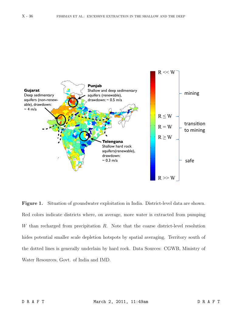
mere 23% in 1985, irrigated area has grown to cover 38% of net sown area in 2001 (see also146

Figure 2). Almost this entire increase is due to irrigation by bore-wells (from 0.3% to 10%147

of net sown area) and shallower dug wells (from about 8% to about 13% of net sown area).148

Bore-well irrigated area has expanded consistently and dramatically, but this expansion149

has been partially eroded by the decline in area irrigated by other sources. The decline in150

areas served by tanks is noteworthy and is attributed to lack of maintenance and siltation151

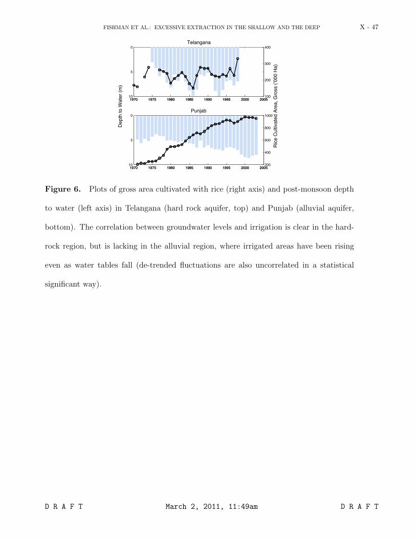
(which is also possibly related to farmers taking up private wells instead). The decline152

in areas irrigated by other wells (dug wells and borecumdug wells, which are bore-wells153

drilled at the bottom of open dug wells) is often also attributed to the expansion of deeper154

tubewells and the resulting lowering of the water table over time.155

The expansion of irrigation is believed to have played a role in the rapid agricultural156

growth in the region in the period of 1970-2001 (see for example Vakulabaharanam [2004]).157



Irrigation allowed the cultivation of waterintensive crops like rice and cotton, the use of158

high yielding varieties (HYVs) and above all, a second cropping during the dry season159

(called the Rabi season, which last from October to March). By the turn of the century,160

Telangana rice production began to rival that of the canal-laden coastal regions (AP is161

one of the major rice growing regions of India) and Rabi season production began to rival162

that of the Kharif season.163

Both Telangana and Punjab are semi-arid regions that employ an energy intensive, rice164

dominated, productive irrigation system that is nevertheless placing great pressure on the165

energy sector (which is both energy starved and required to cross subsidize the basically166

free electricity provided to farmers). In both of them, rice was not cultivated on a large167

scale prior to the advent of groundwater irrigation because of the inadequacy of local168

precipitation. Both of the regions are now classified by the CGWB as over-exploited (i.e.169

Figure 1), and anecdotal reports from both regions tell of drying up and deepening of170

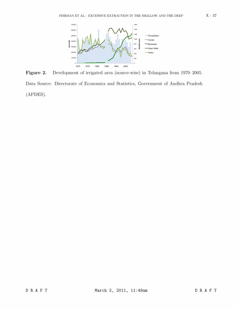
bore-wells. Table 1 highlights some of the basic commonalities and differences between171

the two areas.172

In Punjab, almost the entire cultivated area is irrigated in both seasons (even though173

wheat, which requires far less water, is grown in the dry season). In Telangana, a smaller174

share of the area is irrigated, especially in the dry season. Despite the similarity in175

horsepower and hours of electricity supply, a well in Punjab is able to irrigate a larger176

area, a reflection of the lower hydraulic conductivity and storage capacity of Telangana’s177

fractured granite, in comparison to alluvial strata2. In Punjab, aquifers are vast and deep,178

and the real constraint on irrigation is availability of energy and land. In Telangana, it179

seems that the supply of energy has a more limited capacity in overcoming physical water180



scarcity. The analysis to follow will further confirm this suggestion by showing that the181

high degree of variability in irrigated areas in Telangana over time is driven to a large182

extent by fluctuations in the water table.183

2.2. Groundwater situation

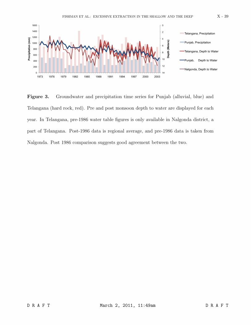
Plots of bi-annual regionally averaged drawdown for Punjab and Telangana are pre-184

sented in Figure 3. Drawdown is measured before (June) and after (November) the annual185

monsoonal recharge season (June-September), during which more than 75 % of the total186

annual rainfall in India is concentrated [Singh et al., 2007]. It is clear, from the figure,187

that the level of recharge is correlated with the amount of precipitation, and that there188

is a large degree of inter-annual variability in both.189

Also, while plots in both regions show the characteristic seesaw pattern of rainy season190

rise and dry season decline, and while the magnitude of the drawdown is comparable,191

there is a clear contrast between the two regions. In Punjab, water table dynamics are192

dominated by a declining trend, the familiar symptom of over-extraction. In Telangana,193

they are dominated by a high degree of short-term fluctuations and there is no clear long-194

term trend. While water tables show a net decline on an average year, the trend can be195

reversed by one or two consecutive wet monsoons that can largely recharge the aquifers.196

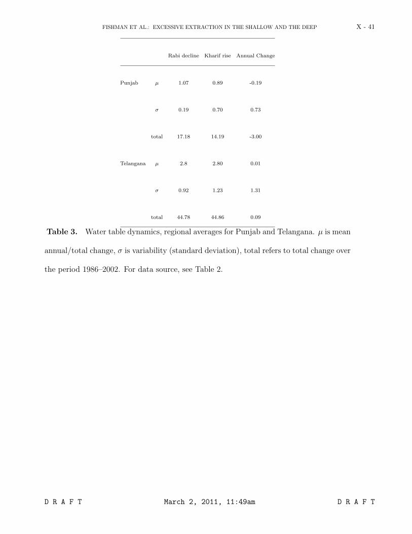
This picture is also reflected in the summary statistics of Table 3.197

In comparison to Punjab, seasonal changes in water tables are larger in Telangana198

(because of both, the higher rainfall and the lower porosity of the strata), but the annual199

decline and rise in drawdown almost cancel out to leave an smaller and insignificant trend200

and a larger degree of variation in annual net change. Finally, it is also interesting to201

note that mean precipitation is higher in Telangana – in fact, it is almost sufficient for202



rice cultivation3. It has to – there is no large reservoir of old water to tap, which is how203

Punjabi farmers are able to cultivate rice with the lower amounts of rainfall. In other204

words, Punjabi rice cultivation relies on the mining of an effectively fossil source of water205

– hence the unsustainable and steady decline in drawdown. Telangana’s irrigation is not206

unsustainable.207

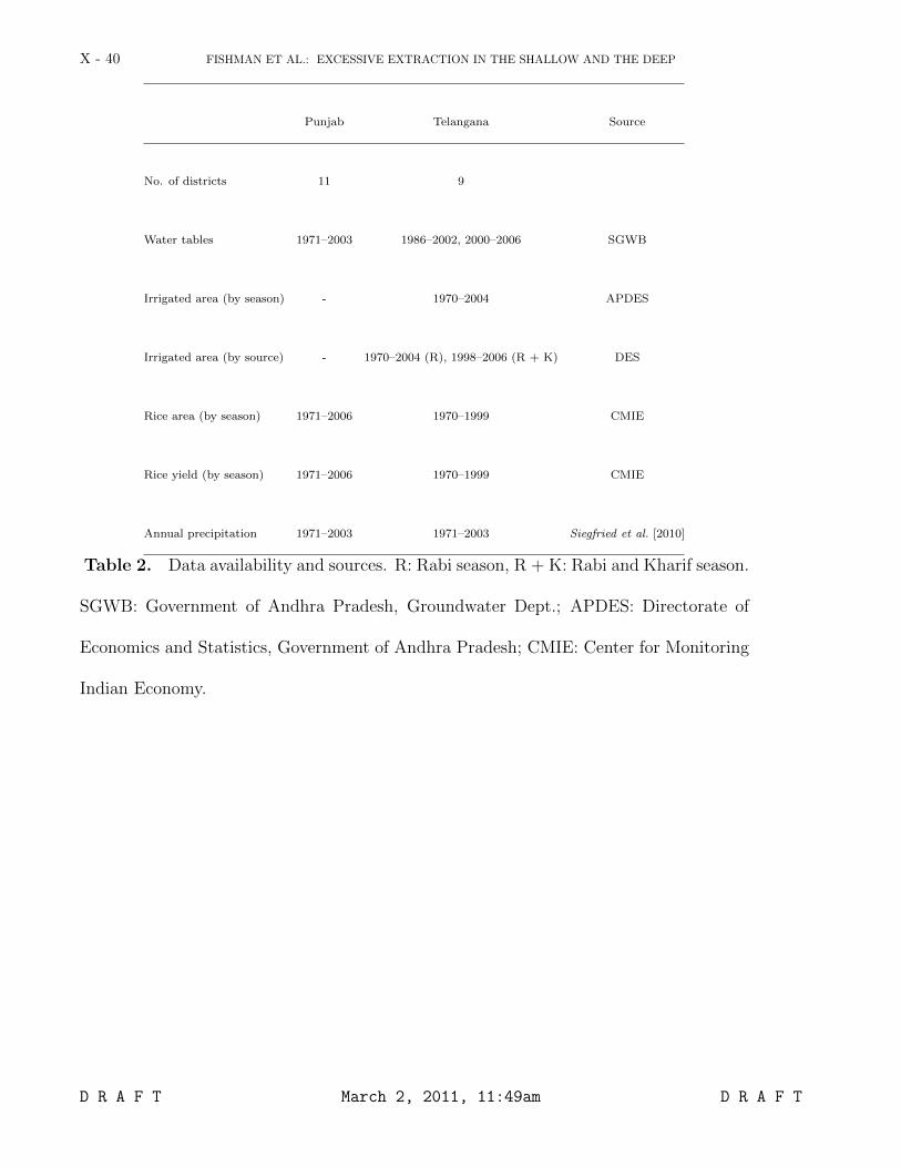
2.3. Data

In both Telangana and Punjab, we use district-level data on irrigated areas, water208

tables (we will use the terms water table, drawdown, or depth to water interchangeably)209

and precipitation. Data are available for the nine districts of Telangana, AP, and for210

eleven districts in Punjab (Table 2 lists all datasets and sources). Annual precipitation211

figures were obtained from a national gridded dataset through a process of weighted spatial212

averaging (for details see Siegfried et al. [2010]). Water table figures were obtained through213

district-wise averaging of data from a network of monitoring wells operated by the state214

groundwater boards of Punjab and Telangana available on a bi-annual basis (pre- and post-215

monsoon). In Punjab, data were obtained for the period 1971–2003 and in Telangana,216

we have data from two separate sets of monitoring wells, one for the period 1986–2002217

and another for the period 1998–20064. We take these averaged water tables as indicators218

of fluctuations rather than absolute value of the water tables actually experienced by219

farmers.220

We focus on agricultural seasons in which land is intensively irrigated, mainly for rice221

cultivation. In Punjab, rice is cultivated only during the rainy season (Kharif). The extent222

of area devoted to irrigated rice cultivation were obtained from from the Indian Harvest223

Database from the Center for Monitoring Indian Economy (2008). In Telangana, details224



of areas irrigated during the rainy Kharif season (net irrigated area) and dry Rabi season225

(area irrigated more than once) were obtained from the Directorate of Economics and226

Statistics, Government of Andhra Pradesh (APDES). In both seasons, a major potion of227

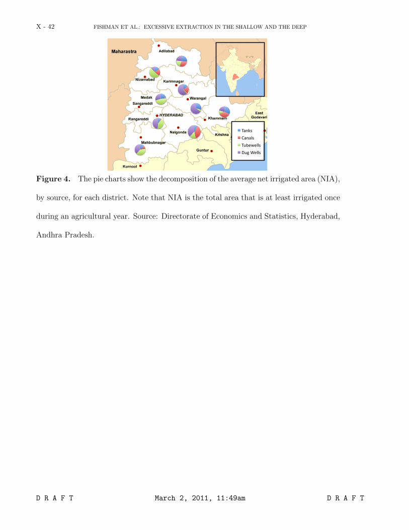
irrigated areas is devoted to rice cultivation. In Telangana, some figures are also available228

on the source-wise decomposition of irrigated areas (only for the rainy season until 1998,229

and for both seasons afterwards). Figure 4 describes the composition of irrigation sources230

in the year 2000.231

3. Water Table Dynamics

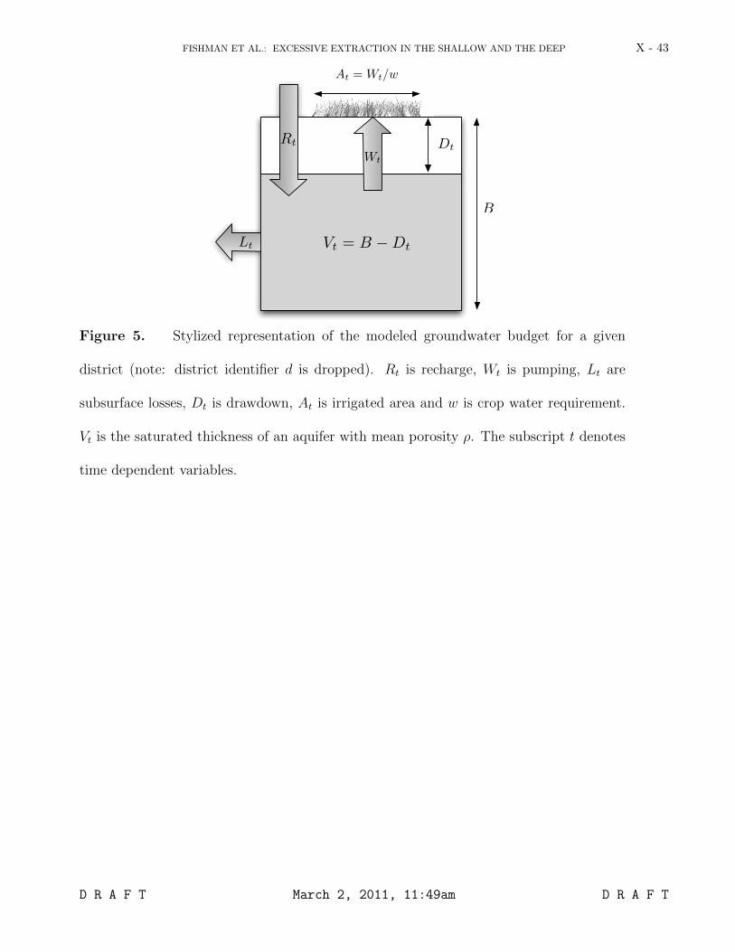
The purpose of the model presented here is to understand annual fluctuations in ground-232

water supply in a given district d. For this purpose, we consider the water budget of a233

simple bathtub aquifer of depth B, the entire surface area (normalized to be one unit) of234

which can cultivated by a given crop with a given water requirement w (Figure 5). This235

aquifer can be an extensive uniform aquifer like those in Punjab, or a much smaller local236

aquifer like those that make up the complex hydrogeology of Telangana. We thus look237

at a fixed spatial extent and ignore trends resulting from an expansion of irrigated area.238

The discrete time step t can refer to a season or to an annual cycle.239

The average depth to water at the beginning of period t in a district d is denoted by Dd,t.240

The volume of water stored in the aquifer at t is Vd,t = ρd(Bd−Dd,t), where ρd is the mean241

porosity which assumed to be uniform and Bd−Dd,t is the saturated thickness at time t.242

Let the amount of water extracted for irrigations net of return flow from excess irrigation243

be Wd,t. Since the average crop water requirement is wd, then area Ad = Wd/wd can be244

irrigated in a given period t. Let the amount of net natural discharge from the aquifer245

that is irretrievably lost to the downstream be Ld,t. Finally, let Pd,t be the in-period t246



precipitation in a particular district. Correspondingly, aquifer recharge from rainfall is247

Rd,t and assumed to be an increasing function of Pd,t.248

The water budget thus becomes249

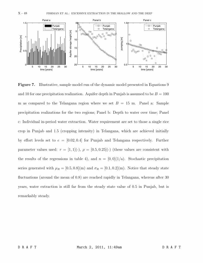
Vd,t+1 = Vd,t −Wd,t − Ld,t +Rd,t (1)

For the reasons outlined in the previous section, we assume that Wd,t and Ld,t are250

functions of the available storage. Hence, under the assumptions251

W = W (V ) ≤ V, L = L(V ) ≤ V (2)

we get252

Vd,t+1 = Vd,t − f(Vd,t) +Rd,t (3)

where f(Vd,t) = W (Vd,t)+L(Vd,t) is a positive, non-decreasing function (we will verify this253

empirically in section 4) of the initial storage V .254

Precipitation, and therefore recharge, fluctuates stochastically in time. We will assume,255

for simplicity, that Pd,t are a sequence of independent and identically distributed random256

variables. Equation 3 therefore describes a stochastic dynamical process. Such a process257

can converge to a steady state. This steady state is itself a probability distribution of258

water tables that is invariant under the dynamics, and if the process is ergodic, describes259

the long-term distribution of water tables over time (see for example Feller [1966]).260

We estimate a linearized version of this process, i.e.261

Vd,t+1 = Vd,t − wVd,t +Rd,t (4)



or, by writing it in terms of observable water tables262

Dd,t+1 = (1− w)Dd,t −r

ρPd,t + cd (5)

where we have assumed that recharge is proportional to precipitation, i.e. Rd,t = rPd,t,263

with r a recharge coefficient, and cd are district specifics constant with cd = wBd. Since264

recharge is always positive, for a stochastic process shown in Equation 5 to converge to a265

steady state, we must have 1 ≥ w ≥ 0.266

We estimate the model by using available water table data from the two regions. In267

each region, water table data is available twice a year (pre-and post monsoon) per district.268

We use the full district-year panel to estimate an ‘average’ regional magnitude of the269

parameters w,r and ρ 5. across the entire panel of observations in each region. Because of270

the high degree of correlation across districts, errors are allowed to be correlated spatially271

(clustered by year).272

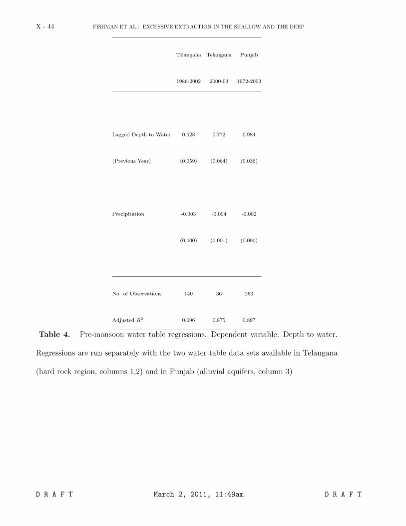
Table 4 displays regression estimates for Telangana (columns 1-2) and Punjab (column273

3) for pre-monsoon (May) water tables6. The estimation suggest, first, that every addi-274

tional mm of rainfall raises the water table by about 3–4 mm in Telangana and by about275

2 mm in Punjab. In terms of physical properties, these estimates should correspond to276

the product of recharge coefficient and porosities in the two regions.277

Second, as shown in Table 4, estimated coefficients on pre-season water tables in Punjab278

are not much different from 1, i.e. w ≈ 0. This suggests that neither extraction nor279

discharge respond strongly to starting depth to water there. In the shallow aquifers280

of Telangana, in contrast, the coefficients are both estimated to be smaller than 1, i.e.281

0 < w < 1 with large probability. This indicates that annual declines in water tables282



are lower when the starting depth to water is deeper. Indeed, the presence of a shallow283

‘bottom’ would reflect in just this way: large declines are simply not possible when the284

water table starts off near to it.285

This interpretation of the results suggests that in Telangana, either discharge or ex-286

traction or both are significantly and negatively associated with the pre-season storage287

(groundwater levels). Put differently, water extraction in this shallow aquifer region is288

limited by water scarcity. In contrast, In the alluvial regions of Punjab, our results suggest289

that extraction is little influenced by water table constraints. There is sufficient supply of290

energy and no physical water constraint, so that the declines in water tables can continue,291

being still far from the physical bottom. In the following section we will use data on292

irrigation to check this directly and confirm these predictions.293

4. Irrigation Dynamics

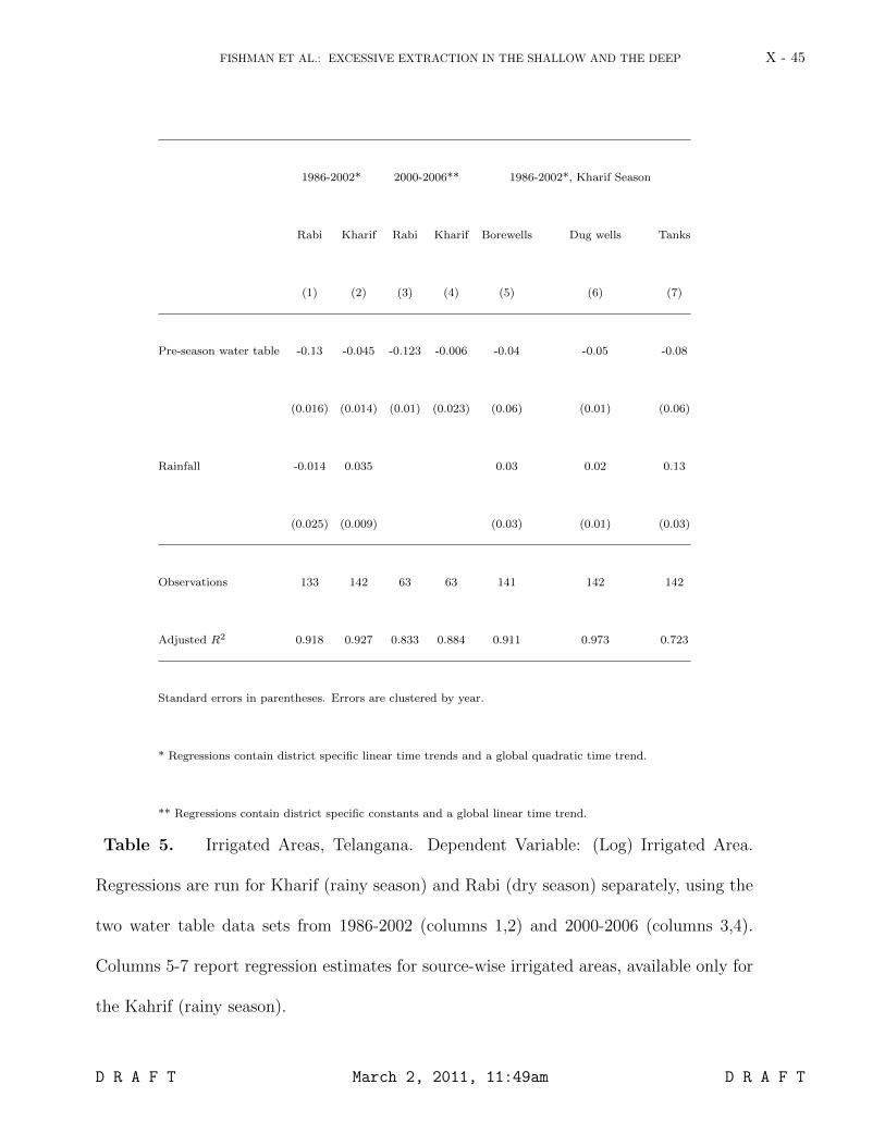
Here, we examine the variation in irrigated area over time and its sensitivity to ground-294

water tables. Since direct measurements of water use are not available we use both total295

irrigated areas (data available in Telangana only) and rice cultivated areas (the principal296

consumer of irrigation water in both regions) as a measure of water use in agriculture.297

Irrigated area provides a good proxy of water availability for irrigation. It is determined298

through cropping choices that are mostly made in the beginning of the agricultural sea-299

son (although it is possible that some of the area is abandoned during the season due300

to either insufficient rainfall, flooding or other factors like pests), and therefore should301

reflect limits on water supply, as perceived by farmers. In fact, it was farmer interviews302

conducted in June 2008 in Nalgonda district (see map Figure 4), that have led us to test303

this relationship. Farmers who wish to maximize the extent of irrigated land will naturally304



prefer to spread the available water supply over as large an area as possible, contingent305

on pre-season water availability. Of course, in making these choices, they may still take306

into account uncertainties in precipitation during the coming rainy season).307

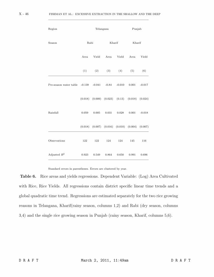
In contrast, the yield of irrigated crops is subject to numerous stochastic influences,308

including the distribution of precipitation, pest outbreaks and solar radiation, to name a309

few, and would thus be a poorer proxy of water availability. Below, we will actually see310

that rice yields are less sensitive to water tables and rainfall than are rice areas.311

Irrigated areas show a great deal of variability in Telangana, a variability that, as we312

will discuss in the next section, can have painful economic implications for farmers. Our313

goal is to assess to what degree this variability is caused by the large fluctuations in water314

tables and precipitation that we studied in the previous section.315

We estimate a model of the form:

log(Ad,t) = −aDd,t + bPd,t + cdt+ log(Ad) + ed,t (6)

Here, Ad,t is area, Dd,t is depth to water, Pd,t is annual (monsoon) rainfall, and Ad are316

unknown base district specific areas, d is a district index and t is a year index. This317

logarithmic model assumes that changes in water tables or rainfall have a scale effect on318

irrigated area, i.e. that the local effects of these variables on irrigated areas on the farm319

level is rather homogenous, and therefore the size of the effect is proportional to the base320

irrigated area in a district. This form is convenient, because it allows us to use a fixed321

effects approach to remove differences in basic scales of irrigation across districts.322

Also, we include district-specific time trends (i.e. district specific growth rates of irri-323

gated areas) in order to isolate annual fluctuations from steady increases that result from324

geographical expansion of irrigation over time7. We also check the robustness of the re-325



sults to the inclusion of quadratic time trends, to the clustering of errors across districts,326

and to AR(1) serial correlation.327

While no data on irrigated area is available for Punjab, such data in Telangana are328

available for the rainy (Kharif) and dry (Rabi) season separately. We run the regressions329

separately over the two periods 1986–2002 and 1998–2006 for which two different water330

table time-series are available. Regressions estimates are displayed in Table 5. The effect331

of the pre-season depth to water has a clear and strong effect in both seasons. A one332

meter decline in depth to water leads to a 13 % reduction in irrigated areas in the dry333

season (consistently across both periods, columns 1 and 3) and a 4.5 % reduction in the334

rainy season (column 2). While annual rainfall is important in the rainy season, and a 100335

mm increase raises irrigated area by 3.5 %, it has no significant effect in the dry season.336

This could reflect either cropping decisions that are based on early season rainfall or the337

abandoning of some irrigated area if precipitation does not fulfill its expected share of the338

water requirements and is consistent with the fact, that rainfall is very highly concentrated339

in the rainy season, so its only effect on the dry season should be mediated through the340

pre-season water table. It is the cumulative rainfall over several years that matters for dry341

season irrigation, not only the same year’s rainfall. In that sense, groundwater resources342

provide a buffer, but this buffering capacity is limited.343

Columns 5-7 in Table 5 display regression estimates for source-wise rainy season irrigated344

areas. Areas irrigated by wells, especially the shallower wells, are mostly responsive to345

water tables, whereas areas irrigated by tanks, shallow surface structures, are especially346

responsive to rainfall. This is consistent with our framework: groundwater irrigation is347



not as sensitive to same year rainfall as small surface storage, but it is sensitive to the348

water table, especially if it comes from shallower wells.349

We also apply similar regressions for the areas cultivated with rice, which dominates350

intensive irrigation in both regions and allows for a comparative analysis. In Punjab, rice351

cultivation is largely restricted to the rainy (Kharif) season, since dry season temperatures352

are unsuitable for it whereas dry season irrigation is devoted to wheat which has an353

approximately 40 % lower irrigation water requirement as compared to rice in the region354

[Bandyopadhyay and Mallick , 2003; Kang et al., 2003]. In Telangana, rice cultivation355

dominates irrigation in both the rainy and dry seasons.356

Regression results, displayed in Table 6, paint a similar pattern as the irrigated area357

regression (Table 5). A one meter decline in the pre-rainy season water table in Telangana358

leads to a 8 % reduction in rice cultivated area. In the dry season, the reduction is larger359

at 14 %. There are no significant effects of either water tables or precipitation in Punjab.360

We also check the effects on rice yields. The effects of rainfall or water tables are sub-361

stantially lower than the corresponding effects on areas, in terms of magnitude, statistical362

significance (except for rainfall during the rainy season in Telangana), and explanatory363

power, consistently with out empirical framework’s focus on areas. In Punjab, rainfall364

actually has a negative effect which is probably attributable to flooding and water logging365

or to reductions in solar radiation, pointing again to the absence of water limitations in366

this region.367

These regression results support the discussion in Section 2 about the relative impor-368

tance of water scarcity and energy in Punjab and Telangana. They are also consistent369

with anecdotal evidence. During the drought years of 1988, 1997 and even 2002, irrigation370



in Telangana suffered greatly and our interviews in the region have revealed that many371

farmers had to abandon their farms and migrate, whereas in Punjab the effect was hardly372

noticeable. Since water tables in Telangana’s hard rock aquifers are highly variable even373

on small spatial scales, deeper average water tables may mean a greater proportion of wells374

are completely dry at the beginning of the season so their owners have to forgo irrigated375

cultivation. Moreover, the interviews showed that farmers gauge pre-season water tables376

and take them into account in deciding how much area to sow with paddy, especially in377

the dry season, when groundwater is the sole source of irrigation water. The decision in378

the rainy season is more complicated because farmers are facing an uncertain supply from379

rainfall, and it is likely, but not certain that it will both fill their wells and reduce irri-380

gation requirements. Moreover, low or excessive rain might force them to abandon some381

of their cropped areas and this might be reflected in the accounting of irrigated areas.382

Whatever the precise mechanism is, both anecdotal evidence and the above regressions383

paint a similar picture of the important role of physical water scarcity as a limiting factor384

in Telangana and its basically non-existent role in Punjab.385

In summary, we find that in Telangana, irrigation grows at a more variable rate than in386

Punjab, and even despite the limitations of our coarse dataset, we are able to see that a387

significant portion of this variation is explained, in a statistically significant and intuitive388

manner by stochastic changes in water supply (and these explain a large fraction of the389

variation). In the dry season, annual fluctuations are largely driven by pre-season water390

tables, and in the rainy season, by rainfall. In the deep aquifers of Punjab, in contrast,391

such changes do not seem to impact irrigation much.392



5. Welfare and Policy Dimension

Discussions of the social impacts of groundwater over-extraction, in India and gener-393

ally, usually revolve around the long-term threats to the sustainability of agricultural394

production and incomes as a result of falling water tables. In Section 3, we saw that395

over-extraction of deep alluvial aquifers in north-western India has indeed led to consis-396

tent declines in water tables over several decades. Conversely, in a prominent region of397

central India overlying shallow aquifers, a declining trend does not subsist over long-term398

period. Off course, this is a natural consequence of the limited storage of such aquifers.399

Extraction cannot actually exceed renewable supply consistently in the long-run, and wa-400

ter tables cannot, by definition, keep declining, because they relatively rapidly approach401

the bottom, and also, because they are rapidly recovered by abundant rainfall.402

The classification of such aquifers as over-extracted should therefore be interpreted in403

a different light. In what sense, then, can such aquifers be excessively exploited? If the404

issue is not really an issue of sustainability, what are the associated welfare losses?405

While lacking in trend, water table dynamics in the hard rock region display a large406

degree of inter-annual variability. In Section 4, we showed that these fluctuations translate407

to fluctuations in irrigated areas, which in turn lead to a high degree of variability in food408

production and farmers’ incomes. Here, we will argue that beyond a point, increases in409

the extraction effort (the density of wells, energy usage, etc.) of a thin aquifer lead to410

increased variability in water supply. This variability can carry high social costs, and411

it is in this sense that extraction can be excessive. In other words, we argue that it is412

extraction effort that can be excessive, because it enables unrestrained extraction when413

water is abundant, and this increases the variability in water tables and, as a result, the414



variability in water extraction and in irrigation. It is this variability that is the main415

source of social welfare losses associated with excessive extraction effort.416

Inter-annual fluctuations in income can carry heavy social costs, especially in a rural, de-417

veloping country context. The development economics literature documents high income418

variability as a prominent characteristic of rural poverty 8 and demonstrates the adverse,419

direct and indirect effects on consumption, welfare, mean income, investment decisions420

and technology adoption [Morduch, 1994; Townsend , 1994]. The primary cause is that the421

poor often lack access to formal financial mechanisms like insurance or credit that enable422

them to maintain stable consumption in the face of income fluctuations. Traditional, in-423

formal mechanisms for consumption smoothing are prevalent in these environments, but424

they seem to only be able to offer partial protection, and are likely to be ineffective in deal-425

ing with non-idiosyncratic income shocks, i.e. shocks that are covariate across households,426

like the spatially coherent rainfall deficiencies we study here. One direct indication of the427

social importance of income variability in rural India is provided by the government’s428

large-scale efforts to provide farmers with alternative sources of income during times of429

low agricultural productivity, a large fraction of which are climate- and water-related.430

Formally, the social welfare loss associated with variability in agricultural production431

means that the (gross) benefits from groundwater exploitation depend not only on the432

mean supply of irrigation water (positively), but also on its variability (negatively). The433

socially optimal choice of the water extraction effort (i.e. well density and depth, pump434

HP, etc.) involves a balance between energy and infrastructure costs and the net benefits435

of irrigation. Below, we illustrate how this optimal level of effort is affected by the presence436

of variability and show in what sense extraction effort can be excessive.437



We analyze a linear form of the coupled groundwater-agriculture dynamics presented438

in Section 3, in which439

W (V ) = eV (7)

and (assuming natural discharge takes place after extraction)440

L(V ) = n(1− e)V (8)

The assumption of linear discharge (post-human harvesting) is the standard modeling441

assumption in linear reservoir models where n is a response factor. The assumption of442

linear water extraction is also common in the natural resources literature (sometimes443

called the Gordon-Schaffer relationship), where the proportionality constant e is referred444

to as harvesting effort. Here, we understand e as an extraction effort. This parameter is445

constrained to be lower than unity, and reflects the density and depth of wells and the446

energy supply, in terms of both pump horsepower and hours of power supply.447

This way of modeling human harvesting behavior is appropriate for un-regularized com-448

mon property, open-access resources, for which incentives to conserve, or reduce effort449

levels are lacking. It is especially apt in the Indian context, because even the electricity450

for pumping is provided at a flat rate which is independent of actual usage (and even this451

charge has been nullified lately), further reducing the incentives for conservation or reduc-452

tions in use. In this context, the level of extraction effort corresponds to the length of daily453

power distribution by the government, as well as to well density and pump horsepower.454

The irregular supply of power is further reason to fully utilize it when it is available. In-455



deed, all anecdotal evidence suggests farmers utilize all electricity provided to maximize456

their water extraction.457

With these assumptions, the dynamics of water tables and water extraction obey the458

following stochastic dynamics:459

Dt+1 = (1− e− n(1− e))Dt −r

ρRt + (e+ n(1− e))B (9)

Wt = eρ(B −Dt) (10)

This simple model can describe the deep aquifers of Punjab as well as the shallow460

aquifers of Telangana by varying the parameter B correspondingly. Both regions have461

roughly similar water requirements per area (same cropping pattern), w ≈ Wt, and compa-462

rable water tables D, but they differ in aquifer depths where B(Punjab)>> B(Telangana)463

which means that e(Punjab)<< e(Telangana)9.464

Over time, the stochastic dynamics it describes converge to a steady state probability465

distribution of water tables and water supply, a distribution that describes both the466

risk profile of water supply in a given year (far enough in the future) and the temporal467

distribution of water extraction over long time scales.468

The time scale needed to converge to the steady state depends on the parameters of the469

model, and in particular, on the depth to the bottom. As an illustration, Figure 7 displays470

a simulation of the model for two parameterizations that roughly capture the two regions,471

and differ primarily in their depth to bottom B. It is clear that the shallower aquifers472

(low B) reach steady states faster (give a constant level of effort). The steady state is not473

an appropriate description of the dynamics of Punjab’s groundwater irrigation, if only by474

the fact it is still able to consistently support extraction in excess of natural recharge, but475



it can be appropriate for the shallow aquifers of Telangana, as is suggested by Figure 3,476

and on which we now focus.477

The steady state corresponding to a given extraction effort level e is characterized by478

a probability distribution for the water table, and hence for water extraction. Increases479

in effort level affect both the expected value and higher moments of this probability480

distribution. In the linear model, we can obtain closed-form solutions for the expected481

value and variance of water extraction, which we will denote by µW (e) = E(W ) and482

σ2W (e) = V(W ), by taking the expectation and variance of the dynamic equation in the483

infinite time limit, and noting that recharge from rainfall is independent of pre-season484

water table 10. Denoting by µR(e) = E(R) and σ2R(e) = V(R) the mean and variance of485

aquifer recharge, we find:486

µW =eµR

e+ n(1− e) (11)

σ2W =

σ2Re

2

1− (e+ n(1− e))2 (12)

From these expressions, it can be readily shown that both the expectation and variance487

of water extraction increase in effort level, i.e.488

dµW

de≥ 0,

dσWde≥ 0 (13)

A higher extraction capacity enables one to capture more of the annual recharge from489

rainfall and lose less to natural discharge. The expected value of water extraction therefore490

increases in e(unless n = 0). The increase in variability is less obvious. It captures the fact491

that high extraction efforts allow the near emptying of the aquifer even after a relatively492



abundant recharge, which leave no buffer in the aquifer in case a dry year follows. The493

reduction in buffering results in higher variability. In the limit, as effort increases and494

e → 1, all buffering capacity of the aquifer is lost: water extraction is exactly equal to495

recharge, and is as variable as rainfall.496

Figure 8 shows a plot of the mean and the spread of the long-term water extraction for497

two values of n. The benchmark case n = 0 (no natural discharge losses) is instructive,498

and is probably a reasonable approximation in Telangana’s aquifers. In this limit expected499

water extraction µW remains constant at the value of average rainfall recharge µR, even as500

the variability σW keeps increasing. This simply reflects the fact that long-term extraction501

must equal long-term recharge (note that the mean depth does increase with e, but these502

two balance each other in terms of water extraction. Off course, the initial volume of503

water stored in the aquifer can help avoid this long-term mass balance for a while — and504

for quite a long while in a deep aquifer where this initial storage can be very large). At505

this limit, it obviously makes no economic sense to increase extraction effort, even if it506

were costless to do, because it only increases the variability without improving the mean.507

For positive values of n, this is not as obvious, as both the expected level and variance508

of water extraction increase simultaneously. The trade-off between increases in these two509

variables depends on the social welfare function and the degree to which it embodies510

aversion to variability.511

A standard way in economic theory to describe a risk-averse social welfare function512

associated with a randomly distributed water supply, is to use a rising, concave benefit513

function B(W ), and define a gross social welfare function associated with a probability514

distribution of water supply as the expected benefit, GB(e) = Ee(B(W )), where the sub-515



script e indicates that the expectation is taken with respect to the probability distribution516

associated with the steady state reached as a result of extracting water at the effort level517

e. Again, the use of the steady state mean benefit is appropriate for the thin aquifer of518

Telangana since it is reached quite rapidly. 11519

The gross social welfare function is a function of e, the water extraction effort, which520

is a measure of the extent of (private and government financed) expenditure on pumping521

infrastructure and energy supply, and has a cost, which we will assume can be described522

by a convex cost function C(e). The net social benefit from an effort level e is then:523

NB(e) = GB(e)− C(e) (14)

The optimal level of social effort is524

e = argmax NB(e) (15)

Our goal here is to understand the effect of stochastic variability in recharge on the525

optimal level of social effort. In the deterministic case this would amount to optimizing526

NB(e) = Be(W (e))− c(e). The stochasticity of precipitation complicates things because527

varying the level of effort now affects the entire probability distribution of water supply,528

and therefore affects the expected benefit not only through the change in the expected529

water supply, but also in higher moments of the water supply distribution.530

Our linear model in Equation 7 and 8 allowed us to calculate the first two moments of531

the water extraction probability distribution. To build on these results, we will assume532

that the benefit function is quadratic 12 (so it will be a function of only the first two533



moments) and concave, and that the gross benefit function is also concave in effort so it534

has a unique maximum:535

Be(w) = aw − bw2

GB(e) = Ee(B(W ))

= B(Ee(W )) + (Ee(B(W ))−B(Ee(W )))

= B(µW )− bσ2W (16)

We have seen in Equation 12 above that σ2W is proportional to σ2

R, the variance of536

aquifer recharge. The optimal level of effort is determined by the first-order condition:537

dB(µW )

de− bdσ

2W

de=dC(e)

de(17)

Suppose now that σR is increased, i.e. that the variability in aquifer recharge is in-538

creased. This decreases the LHS. To rebalance the equation for the new level of σR, e539

should therefore be lowered, because by assumption of concavity that would increase the540

LHS and decrease the RHS. Thus, the new optimal level of effort becomes lower. This541

proves that, in our linearized model, the optimal level of extraction effort e is decreasing542

in the variability of rainfall. In particular, it is lower than the deterministic optimal level.543

This is intuitively pleasing. Once again, a higher extraction effort reduces the losses544

to natural discharge, but reduces the reliability of water extraction. Taking this into545

consideration reduces the socially optimal level of harvesting effort. This is the key insight546

of our model.547

6. Discussion and Conclusion



By mining the large volumes of stored water, and by continuously enhancing extrac-548

tion capacity through increases in the depth of wells and the power of pumps, Punjabi549

agriculture can temporarily sustain water use levels that exceeds mean recharge, escape550

the long-run mass balance and remain far from steady state. Eventually, this process551

will come to a halt. Extraction capacity will hit a practical (the energy or drilling costs552

become prohibitive) or theoretical limit (maximum effort reached) and water extraction553

will start to decline and the system will converge to a steady state, but this outcome does554

not seem to be very near in Punjab.555

In Telangana, however, the shallowness of the aquifer means convergence to steady556

state is rapid so the steady state can provide a reasonable approximation. Increases in557

extraction capacity can sometimes raise water supply above mean recharge, but this will558

be a short-lived benefit. In the long-run, as our model shows, such increases will improve559

the mean (at a decreasing rate), and they will also reduce the buffering capacity of the560

irrigation system and its reliability. The length of the time-series we have is insufficient561

to establish these predictions empirically, but the general pattern suggested by Figure 2 is562

not inconsistent with them. The boom in bore-well proliferation (an increase in extraction563

capacity) has had some positive returns, but they are not as high as would be hoped and564

they have certainly not made the groundwater irrigated agricultural system more reliable565

or steady.566

The lack of regulation on groundwater pumping and structuring of the costs of energy567

in much of India, including our regions of study in Punjab and Andhra Pradesh, makes568

it unlikely that the socially optimal level of extraction effort, as discussed above, will be569

achieved. First, electricity for pumping is provided at no cost in the two states (elsewhere570



in India the rate is flat and highly subsidized). Farmers do not face a marginal cost of571

neither pumping energy nor groundwater and have little incentive to use it efficiently,572

especially as they are locked in a tragedy of the commons over the exploitation of this573

common resource. Under these conditions, it is natural for farmers to use as much energy574

as their pumps can use while it is supplied, which is sure to be excessive from the social575

point of view. Second, while farmers do bear the costs of installing wells, the open access576

to the groundwater resource suggests there is an excess of wells being drilled and that577

erodes the water supply and profit per well (for more discussion on that topic, see also578

Athanassoglou et al. [2011]). For these two reasons, it is likely that extraction capacity is579

excessive, even if only from the point of view of average profit.580

Even if the costs of enhanced variability are ignored, there are good reasons to ex-581

pect extraction capacity to be excessive, in other ways, in both Punjab and Telangana.582

Groundwater is a common, free access resource. There is no real limitation or regulation583

on the drilling of wells to access it. Basic economic principles predicts inefficiently ex-584

cessive extraction capacity to be installed in exploiting such an open access resource, in585

the sense that the mean returns per unit of effort (i.e. per well, or per unit of energy)586

will be lower than optimum. To make matters worse, in both the states, Andhra Pradesh587

and Punjab, as in most key groundwater irrigated parts of India, energy costs are heavily588

subsidized by state governments and the low tariffs are also flat, so there is no marginal589

cost on the use of pumping energy, not to speak of water.590

The analysis in this paper suggests there are additional costs to this excessive extraction591

capacity because of the variability it enhances. Not only is extraction capacity inefficiently592

excessive in terms of average profits, but in shallow aquifers like Telangana’s, our model593



suggests it may lead to an increase in variability that further reduces social welfare. Our594

analysis thus provides additional motivation for reducing energy use in Indian agriculture.595

It may not be unreasonable for a government to find it justified to spend large amounts of596

energy in order to sustain irrigation, support rural livelihood and boost food production.597

However, our analysis shows that even if the government’s energy costs are ignored, a598

large energy supply may actually harm the welfare of the farmers that utilize it in ways599

that have not been appreciated so far.600

Acknowledgments. Support from the Pepsi Co. foundation and the Columbia Uni-601

versity’s Cross-Cutting Initiative at the Earth Institute is gratefully acknowledged. We602

would like to dedicate this paper to the memory of Dr. Pradeep Raj who passed away603

early 2011. Dr. Raj was instrumental in furthering our understanding of the groundwater604

situation in India. We are grateful to him for having been a constant source of inspiration605

and learning. He will be deeply missed. We thank Victor Vazquez. We thank S. P. Tucker606

and the district collector of Nalgonda District. We thank the Groundwater department,607

Government of Andhra Pradesh and Nalgonda district, as well as the Andhra Pradesh608

directorate of Economics and Statistics, for helpful discussions and data. We offer special609

thanks to A. C. Reddy for assistance and insights in the field. We thank the participants610

of the 11th Occasional California Workshop on Environmental and Resource Economics,611

University of California Santa Barbara, the Eleventh Annual Colorado University Environ-612

mental and Resource Economics Workshop, Vail, Colorado, the Sustainable Development613

seminar at Columbia University, New York and sessions in the American Geophysical614

Union meetings in San Francisco, 2009, for helpful discussions.615



Notes

1. While reliable figures are difficult to come by, it is clear that energy use for pumping has increased steadily over the last

few decades [Morris, 1996; Dubash, 2008] and in many states it is estimated to use more than 40 % of total electricity

consumption and be responsible for more than 40% of the annual budget deficit [Briscoe et al., 2006].616

2. The hydraulic conductivity of granite is in the order of 10−7 ft/day (even though it is highly variable and can locally be

as high as 10 − 103 ft/day) whereas in an alluvium it is in the range 0.1 − 103 ft/day [Raj et al., 1996; Raj , 2004b].

3. Off course, a smaller fraction of the total land area is irrigated in Telangana, but on the other hand, only a fraction of

precipitation over unirrigated land is actually captured for recharging the aquifer.

4. It should be noted that water tables reported by monitoring wells tend to be lower than those reported by farmers in

their irrigation wells, probably due to local cones of depression around active irrigation wells.

5. Each of our two regions is relatively homogenous in its hydro-geologic properties, but the two regions are very different

from one another

6. Note that regressions for post-monsoon water tables (not shown) produce similar results.

7. Growth in irrigated areas can take place on both the extensive and intensive margin. The spread of irrigation wells to

new locations extends irrigation geographically, whereas an increase in the supply of energy can increase the yield of an

existing well. Remarkably, the rise of irrigated areas in Punjab coincides with the steady decline in water tables and the

associated rise in the amount of energy required to lift a given amount of water. The method of paddy cultivation makes

it unlikely that the intensity of irrigation has been improving in any significant manner, so the spread of irrigation is

likely driven by an even steeper increase in energy use for pumping.

In Telangana, where hard rock aquifers are more localized and heterogeneous, the geographical expansion of wells

can exploit new pockets of groundwater so it is probably the more potent driver of the expansion of irrigation. This is

especially true if, as suggested in the introduction, irrigation there is constrained by water scarcity, rather than land or

energy limitations: an increase in the energy supply per well should do little to increase the supply of water beyond a

temporary access to hitherto untapped layers of water through a deeper, more energized well. Figure 2 suggests that is

part of what happened when bore-wells were introduced in Telangana: the rise in areas irrigated by bore-wells was soon

followed by a decline (and larger fluctuations) in areas served by the traditional, shallow, open dug wells.

8. Some of the original evidence comes from the same areas we are analyzing here, e.g. [Walker and Ryan, 1990]

9. Indeed, in this linear model, the estimates of Section 4, mean that in Punjab e + n(1 − e) << 1, whereas in Telangana

e+ n(1 − e) is not negligible. Note also that in this linear model, we have, to first order, Wt+1/Wt ≈ 1 + ∆D/B, so the

coefficients of log irrigated areas on water tables can be interpreted as the inverses of some effective depth of the aquifer:

this is consistent with the comparison of Punjab and Telangana (Table 6) as well as the comparison of different irrigation

sources within Telangana (Table 5).



10.It should be noted that in this approximation the model does not prevent the aquifer from spilling over which implies

that negative values of D might occur artificially. Hence, e must be at least high enough to guarantee that E(D) > 0 for

the model to be meaningful, i.e. that Be(e+n) > R, so that natural losses plus extraction exceed mean recharge. Lower

values of e lead to rising water tables, i.e. a regime that is far removed from the realities of both of our regions

11.This approach would not be appropriate for thick aquifers where it only describes the long-term distribution and therefore

needs to be balanced with short-term benefits in an inter-temporal optimality framework. We do not engage in such

analysis in this paper. It has been extensively discussed in the groundwater economics literature (see [Rubio and Casino,

2001] for a review), and our focus here is different.

12.As an example of a welfare function that describes one of the harmful effect of variability, consider the market price p of

irrigated crop production F assumed to be proportional to the water supply in any year. This market price is negatively

related to the supply F , and it is standard to assume a linear relationship p = p0 − ρF . The annual profit from irrigated

cultivation is pF = p0F −aF 2. The expected (or mean long-term) profit is reduced when variability is increased (keeping

the expected value constant), since prices and production are negatively correlated E(pF ) ≤ E(p)E(F ) and the difference

is higher the more variable F is.

References

Athanassoglou, S., G. Sheriff, T. Siegfried, and T. Huh, A simple mechanism for a complex617

aquifer, 2011, mimeo.618

Bandyopadhyay, P., and S. Mallick, Actual evapotranspiration and crop coefficients of619

wheat (triticum aestivum) under varying moisture levels of humid tropical canal com-620

mand area, Agricultural Water Management , 59 , 33–47, 2003.621

Briscoe, J., R. Malik, and W. Bank, India’s Water Economy: Bracing for a turbulent622

future, Oxford University Press, 2006.623

Central Ground Water Board, Annual report, 2006-2007, Tech. rep., Ministry of Water624

Resources, Govt. of India, Faridabad, 2007.625

Dubash, N. K., The electricity-groundwater conundrum: Case for a political solution to626

a political problem, Economic and Political Weekly , 2008.627



Feller, W., An Introduction to Probability Theory and Its Applications , vol. 2, 3 ed., Wiley,628

1966.629

Kang, S., B. Gu, T. Du, and J. Zhang, Crop coefficient and ratio of transpiration to630

evapotranspiration of winter wheat and maize in a semi-humid region, Agricultural631

Water Management , 59 , 239–254, 2003.632

Kumar, M., K. Kumari, A. Ramanathan, and R. Saxena, A comparative evaluation of633

groundwater suitability for irrigation and drinking purposes in two intensively cultivated634

districts of Punjab, India, Environmental Geology , 53 , 553–574, 2007.635

Moench, M., Drawing down the buffer: Science and politics of ground water management636

in india, Economic and Political Weekly , 27 , 7–14, 1992.637

Morduch, J., Poverty and vulnerability, The American Economic Review , 84 , 221–225,638

1994.639

Morris, S., Political economy of electric power in india, Economic and Political Weekly ,640

31 , pp. 1274–1285, 1996.641

Raj, P., Groundwater Resource, 2004-05, Andhra Pradesh, Tech. rep., Groundwater De-642

partment, Government of Andhra Pradesh, 2004a.643

Raj, P., Classification and interpretation of piezometer well hydrographs in parts of south-644

eastern peninsular india, Environmental Geology , 46 , 808–819, 2004b.645

Raj, P., Status of ground water in Andhra Pradesh: Availability, Use and Strategies for646

Management, Tech. rep., Groundwater Department, Government of Andhra Pradesh,647

India, 2006.648

Raj, P., L. Nandulal, and G. Soni, Nature of aquifer in parts of granitic terrain Mahabub-649

nagar District, Andhra Pradesh, Journal of the Geological Society of India, 49 , 61–74,650



1996.651

Ribot, J., A. Magalhaes, and S. Panagides, Climate variability, climate change and social652

vulnerability in the semi-arid tropics , Cambridge Univ Pr, 1996.653

Rodell, M., I. Velicogna, and J. Famiglietti, Satellite-based estimates of groundwater654

depletion in india, Nature, 460 , 999–1002, 2009.655

Rubio, S. J., and B. Casino, Competitive versus efficient extraction of a common property656

resource: The groundwater case, Journal of Economic Dynamics and Control , 25 , 1117657

– 1137, 2001.658

Shah, T., Taming the Anarchy: Groundwater Governance in South Asia, RFF Press,659

2008.660

Shiklomanov, I. A., Appraisal and Assessment of World Water Resources, Water Inter-661

national , 25 , 11–32, 2000.662

Siegfried, T., S. Sobolowski, P. Raj, R. Fishman, V. Vasquez, K. Narula, U. Lall, and663

V. Modi, Modeling Irrigated Area to Increase Water, Energy and Food Security in664

Semi-Arid India, Weather, Climate, and Society , 2010.665

Singh, K. K., D. R. Reddy, S. Kaushik, L. S. Rathore, J. Hansen, and G. Sreenivas,666

Application of Seasonal Climate Forecasts for Sustainable Agricultural Production in667

Telangana Subdivision of Andhra Pradesh, India, Springer Berlin Heidelberg, 2007.668

The World Bank and Government of India, India – water resources management sector669

review: Groundwater regulation and management report., Tech. rep., World Bank,670

Government of India, Washington, DC, New Delhi, 1980.671

Tiwari, V., J. Wahr, and S. Swenson, Dwindling groundwater resources in northern india,672

from satellite gravity observations, Geophysical Research Letters , 36 , L18,401, 2009.673



Townsend, R., Risk and insurance in village india, Econometrica: Journal of the Econo-674

metric Society , 62 , 539–591, 1994.675

UNDP, Human Development Report , UNDP, United Nations Development Programme,676

2006.677

Vakulabaharanam, V., Agricultural Growth and Irrigation in Telangana: A Review of678

Evidence, Economic and Political Weekly , 2004.679

Wada, Y., L. van Beek, C. van Kempen, J. Reckman, S. Vasak, and M. Bierkens, Global680

depletion of groundwater resources, Geophysical Research Letters , 37 , 2010.681

Walker, T., and J. Ryan, Village and household economies in India’s semi-arid tropics ,682

Baltimore, Maryland, USA: Johns Hopkins University Press. 420pp. ISBN 0-8018-3886-683

X, 1990.684



R << W

R ! W

R " W

R >> W

R = W

!"#"#$

%&'(

)*&#%"+,#-),-!"#"#$

PunjabShallow and deep sedimentary aquifers (renewable), drawdown: ~ 0.5 m/a

GujaratDeep sedimentary aquifers (non-renew-able), drawdown: ~ 4 m/a

TelenganaShallow hard rock aquifers(renewable), drawdown:~ 0.3 m/a

Figure 1. Situation of groundwater exploitation in India. District-level data are shown.

Red colors indicate districts where, on average, more water is extracted from pumping

W than recharged from precipitation R. Note that the coarse district-level resolution

hides potential smaller scale depletion hotspots by spatial averaging. Territory south of

the dotted lines is generally underlain by hard rock. Data Sources: CGWB, Ministry of

Water Resources, Govt. of India and IMD.



0

200

400

600

800

1000

1200

1400

1600

0

100000

200000

300000

400000

500000

600000

700000

1970 1976 1982 1988 1994 2000

Rai

nfal

l (m

m)

Are

a (H

a)

Precipitation

Canals

Borewells

Open Wells

Tanks

Figure 2. Development of irrigated area (source-wise) in Telangana from 1970–2005.

Data Source: Directorate of Economics and Statistics, Government of Andhra Pradesh

(APDES).



Punjab Telangana

Average hours of electricity supply 6.2 6.6

Average pump horsepower 5.4 4.7

Costs of electricity for pumping free free

Principal water consumer rice rice

Hydrogeology alluvial hard rock

Precent of area irrigated (from groundwater) 94% (68%) 41% (43%) (AP)

Area irrigated per well, Kharif Season 2.6 (rice +) 0.8 (rice +)

Area irrigated per well, Rabi Season 2.6 (rice +) 0.5 (rice +)

Table 1. Key irrigation characteristics in Punjab and Telangana. Source: 3rd Census

of Minor Irrigation Schemes.



0

2

4

6

8

10

12

14 0

200

400

600

800

1000

1200

1400

1600

1973 1976 1979 1982 1985 1988 1991 1994 1997 2000 2003

Dep

th (M

eter

s)

Pre

cipi

tatio

n (m

m)

Telangana, Precipitation

Punjab, Precipitation

Telangana, Depth to Water

Punjab, Depth to Water

Nalgonda, Depth to Water

Figure 3. Groundwater and precipitation time series for Punjab (alluvial, blue) and

Telangana (hard rock, red). Pre and post monsoon depth to water are displayed for each

year. In Telangana, pre-1986 water table figures is only available in Nalgonda district, a

part of Telangana. Post-1986 data is regional average, and pre-1986 data is taken from

Nalgonda. Post 1986 comparison suggests good agreement between the two.



Punjab Telangana Source

No. of districts 11 9

Water tables 1971–2003 1986–2002, 2000–2006 SGWB

Irrigated area (by season) - 1970–2004 APDES

Irrigated area (by source) - 1970–2004 (R), 1998–2006 (R + K) DES

Rice area (by season) 1971–2006 1970–1999 CMIE

Rice yield (by season) 1971–2006 1970–1999 CMIE

Annual precipitation 1971–2003 1971–2003 Siegfried et al. [2010]

Table 2. Data availability and sources. R: Rabi season, R + K: Rabi and Kharif season.

SGWB: Government of Andhra Pradesh, Groundwater Dept.; APDES: Directorate of

Economics and Statistics, Government of Andhra Pradesh; CMIE: Center for Monitoring

Indian Economy.



Rabi decline Kharif rise Annual Change

Punjab µ 1.07 0.89 -0.19

σ 0.19 0.70 0.73

total 17.18 14.19 -3.00

Telangana µ 2.8 2.80 0.01

σ 0.92 1.23 1.31

total 44.78 44.86 0.09

Table 3. Water table dynamics, regional averages for Punjab and Telangana. µ is mean

annual/total change, σ is variability (standard deviation), total refers to total change over

the period 1986–2002. For data source, see Table 2.



!"#$%&

'"#"(%&

!)*+,+((%&

-).&/+((%&

Figure 4. The pie charts show the decomposition of the average net irrigated area (NIA),

by source, for each district. Note that NIA is the total area that is at least irrigated once

during an agricultural year. Source: Directorate of Economics and Statistics, Hyderabad,

Andhra Pradesh.



Vt = B − Dt

Rt

Lt

B

Dt

At = Wt/w

Wt

Figure 5. Stylized representation of the modeled groundwater budget for a given

district (note: district identifier d is dropped). Rt is recharge, Wt is pumping, Lt are

subsurface losses, Dt is drawdown, At is irrigated area and w is crop water requirement.

Vt is the saturated thickness of an aquifer with mean porosity ρ. The subscript t denotes

time dependent variables.



Telangana Telangana Punjab

1986-2002 2000-03 1972-2003

Lagged Depth to Water 0.528 0.772 0.984

(Previous Year) (0.059) (0.064) (0.036)

Precipitation -0.003 -0.004 -0.002

(0.000) (0.001) (0.000)

No. of Observations 140 36 263

Adjusted R2 0.696 0.875 0.897

Table 4. Pre-monsoon water table regressions. Dependent variable: Depth to water.

Regressions are run separately with the two water table data sets available in Telangana

(hard rock region, columns 1,2) and in Punjab (alluvial aquifers, column 3)



1986-2002* 2000-2006** 1986-2002*, Kharif Season

Rabi Kharif Rabi Kharif Borewells Dug wells Tanks

(1) (2) (3) (4) (5) (6) (7)

Pre-season water table -0.13 -0.045 -0.123 -0.006 -0.04 -0.05 -0.08

(0.016) (0.014) (0.01) (0.023) (0.06) (0.01) (0.06)

Rainfall -0.014 0.035 0.03 0.02 0.13

(0.025) (0.009) (0.03) (0.01) (0.03)

Observations 133 142 63 63 141 142 142

Adjusted R2 0.918 0.927 0.833 0.884 0.911 0.973 0.723

Standard errors in parentheses. Errors are clustered by year.

* Regressions contain district specific linear time trends and a global quadratic time trend.

** Regressions contain district specific constants and a global linear time trend.

Table 5. Irrigated Areas, Telangana. Dependent Variable: (Log) Irrigated Area.

Regressions are run for Kharif (rainy season) and Rabi (dry season) separately, using the

two water table data sets from 1986-2002 (columns 1,2) and 2000-2006 (columns 3,4).

Columns 5-7 report regression estimates for source-wise irrigated areas, available only for

the Kahrif (rainy season).



Region Telangana Punjab

Season Rabi Kharif Kharif

Area Yield Area Yield Area Yield

(1) (2) (3) (4) (5) (6)

Pre-season water table -0.139 -0.041 -0.84 -0.010 0.001 -0.017

(0.018) (0.009) (0.023) (0.13) (0.018) (0.024)

Rainfall 0.059 0.005 0.031 0.028 0.001 -0.018

(0.018) (0.007) (0.016) (0.010) (0.004) (0.007)

Observations 122 122 124 124 145 116

Adjusted R2 0.923 0.549 0.864 0.650 0.991 0.696

Standard errors in parentheses. Errors are clustered by year.

Table 6. Rice areas and yields regressions. Dependent Variable: (Log) Area Cultivated

with Rice, Rice Yields. All regressions contain district specific linear time trends and a

global quadratic time trend. Regressions are estimated separately for the two rice growing

reasons in Telangana, Kharif(rainy season, columns 1,2) and Rabi (dry season, columns

3,4) and the single rice growing season in Punjab (rainy season, Kharif, columns 5,6).



1970 1975 1980 1985 1990 1995 2000 200510

5

0

Dep

th to

Wat

er (m

)

1970 1975 1980 1985 1990 1995 2000 2005100

200

300

400

Ric

e C

ultiv

ated

Are

a, G

ross

(’00

0 H

a)

Telangana

1970 1975 1980 1985 1990 1995 2000 200510

5

0

1970 1975 1980 1985 1990 1995 2000 2005200

400

600

800

1000Punjab

Figure 6. Plots of gross area cultivated with rice (right axis) and post-monsoon depth

to water (left axis) in Telangana (hard rock aquifer, top) and Punjab (alluvial aquifer,

bottom). The correlation between groundwater levels and irrigation is clear in the hard-

rock region, but is lacking in the alluvial region, where irrigated areas have been rising

even as water tables fall (de-trended fluctuations are also uncorrelated in a statistical

significant way).



5 10 15 20 25 300

0.5

1

1.5

time [years]

Prec

ipita

tion

[m]

Panel a

PunjabTelangana

5 10 15 20 25 3025

20

15

10

5

0

time [years]Aq

uife

r sto

rage

hei

ght [

m]

Panel b

PunjabTelangana

5 10 15 20 25 300.5

1

1.5

time [years]

pum

ping

[m]

Panel c

PunjabTelangana

Figure 7. Illustrative, sample model run of the dynamic model presented in Equations 9

and 10 for one precipitation realization. Aquifer depth in Punjab is assumed to be B = 100

m as compared to the Telangana region where we set B = 15 m. Panel a: Sample

precipitation realizations for the two regions; Panel b: Depth to water over time; Panel

c: Individual in-period water extraction. Water requirement are set to those a single rice

crop in Punjab and 1.5 (cropping intensity) in Telangana, which are achieved initially

by effort levels set to e = [0.02, 0.4] for Punjab and Telangana respectively. Further

parameter values used: r = [1, 1](-), ρ = [0.5, 0.25](-) (these values are consistent with

the results of the regressions in table 4), and n = [0, 0](1/a). Stochastic precipitation

series generated with µR = [0.5, 0.8](m) and σR = [0.1, 0.2](m). Notice that steady state

fluctuations (around the mean of 0.8) are reached rapidly in Telangana, whereas after 30

years, water extraction is still far from the steady state value of 0.5 in Punjab, but is

remarkably steady.



0 0.1 0.2 0.3 0.4 0.5 0.6 0.7 0.8 0.9 10

0.1

0.2

0.3

0.4

0.5

0.6

0.7

0.8

0.9

1

Level of e!ort e

µW

Panel a

2!W (n = 0)µW (n = 0)2!W (n = 0.1)µW (n = 0.1)

Figure 8. The Figure shows the steady state mean (dotted line) and spread (standard

deviation, shaded area) of groundwater supply as a function of extraction effort levels e

(see Equations 11 and 12) for the Telangana region, using the parameterization of Figure

7. Two different parameter values for n are shown. n = 0 is the case where water losses

L to the downstream are negligible.


Date post:	27-May-2020
Category:	Documents
Upload:	others
View:	28 times
Download:	0 times

Over-Extraction in the Shallow and the Deep { The...1 Over-Extraction in the Shallow and the Deep {...

Documents