Overcoming Computational Challenges on Large Scale Overcoming Computational Challenges on Large Scale Overcoming Computational Challenges on Large Scale Overcoming Computational Challenges on Large Scale Security Constrained Unit Commitment (SCUC) Problems Security Constrained Unit Commitment (SCUC) Problems Security Constrained Unit Commitment (SCUC) Problems Security Constrained Unit Commitment (SCUC) Problems – – – MISO and Alstom’s Experience with MIP Solver MISO and Alstom’s Experience with MIP Solver MISO and Alstom’s Experience with MIP Solver MISO and Alstom’s Experience with MIP Solver Yonghong Chen, Principal Advisor, MISO Xing Wang, R&D Director, Alstom Grid Qianfan Wang, Power System Engineer, Alstom Grid FERC Technical Conference on Increasing Real-Time and Day-Ahead Market Efficiency through Improved Software, June 23-25, 2014
Transcript
Overcoming Computational Challenges on Large Scale Overcoming Computational Challenges on Large Scale Overcoming Computational Challenges on Large Scale Overcoming Computational Challenges on Large Scale Security Constrained Unit Commitment (SCUC) Problems Security Constrained Unit Commitment (SCUC) Problems Security Constrained Unit Commitment (SCUC) Problems Security Constrained Unit Commitment (SCUC) Problems
–––– MISO and Alstom’s Experience with MIP SolverMISO and Alstom’s Experience with MIP SolverMISO and Alstom’s Experience with MIP SolverMISO and Alstom’s Experience with MIP Solver
Yonghong Chen, Principal Advisor, MISO
Xing Wang, R&D Director, Alstom Grid
Qianfan Wang, Power System Engineer, Alstom Grid
FERC Technical Conference on Increasing Real-Time and Day-Ahead Market Efficiency through
Improved Software, June 23-25, 2014
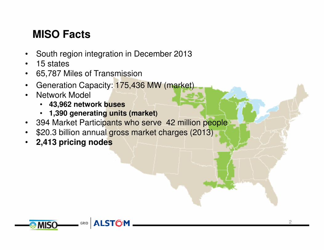
MISO Facts
• South region integration in December 2013• 15 states• 65,787 Miles of Transmission
• Generation Capacity: 175,436 MW (market)• Network Model
• 43,962 network buses
• 1,390 generating units (market)
• 394 Market Participants who serve 42 million people• $20.3 billion annual gross market charges (2013)• 2,413 pricing nodes
2
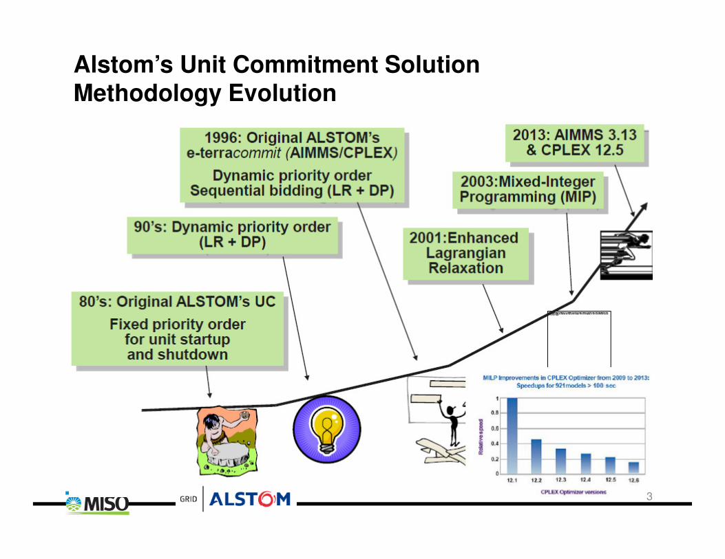
Alstom’s Unit Commitment Solution Methodology Evolution
3
MISO SCUC
• Energy only market started in 2005– Lagrangian Relaxation (LR) based SCUC from Alstom
• Co-optimized energy and ancillary service market launched in 2009– Transition to SCUC using CPLEX MIP solver
• Commercial solver has made the efficient market expansion and market enhancement possible – Focus more on developing good mathematic models and formulations
to reflect market rules and meet business needs • Launch of co-optimized energy and ancillary service market • Integration of south region• Market enhancement projects implemented, e.g.
– Look-ahead commitment (LAC)– Post zonal reserve deployment transmission constraints to address reserve
deliverability issues– Performance based regulation compensation (FERC Order 755)
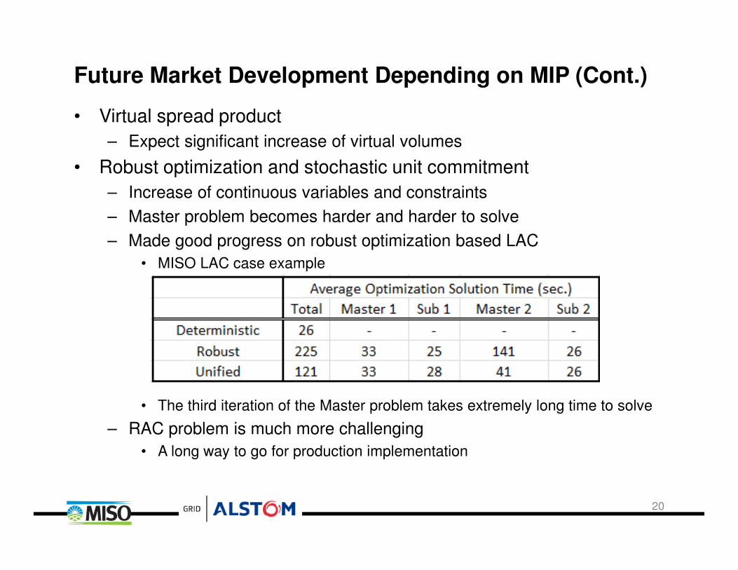
• Market development prototypes, e.g.– Configuration based combined cycle model– Robust optimization based LAC
• MIP solver can solve very well within required time limits for mostcases. However, for a very small percentage of cases, it mayhave difficulty to find good solutions and require longer time tosolve.
4
MISO SCUC Model
• Identified factors that drive MIP performance challenges
– Number of binary and continuous variables
– Number of transmission constraints
– Density of matrix
– Required solving time
• MISO has one of the largest and most complicated unit commitment problems in the real world
– Commitment process
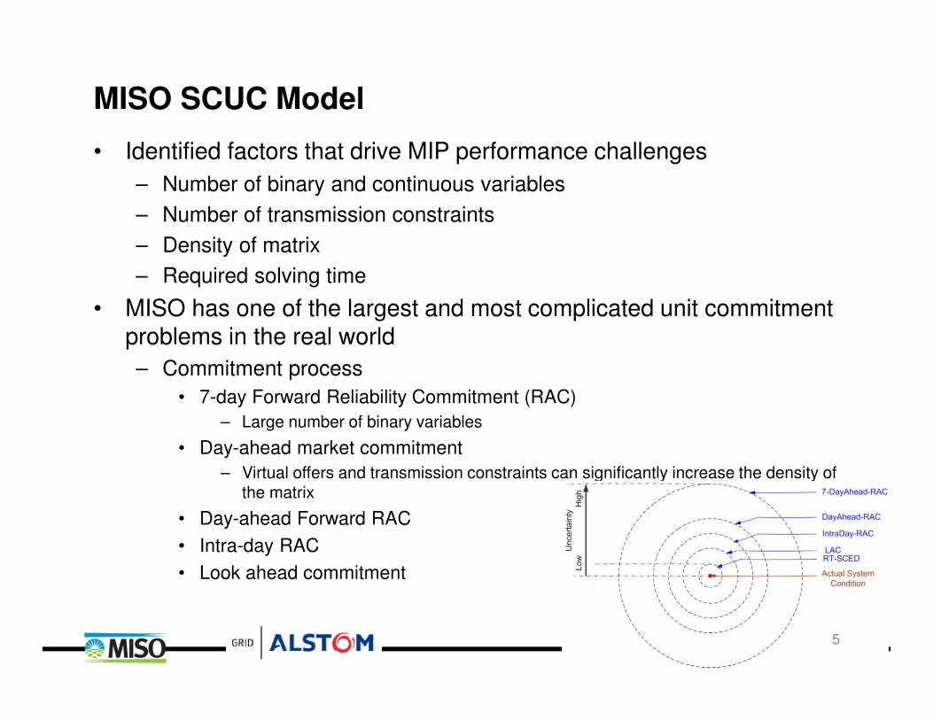
• 7-day Forward Reliability Commitment (RAC)
– Large number of binary variables
• Day-ahead market commitment
– Virtual offers and transmission constraints can significantly increase the density of the matrix
• Day-ahead Forward RAC
• Intra-day RAC
• Look ahead commitment
5
MIP Solver based SCUC
• MIP solvers
– “Branch & bound” + “heuristics”
– Solution and lower bound
• MIP gap to indicate the quality of the solution
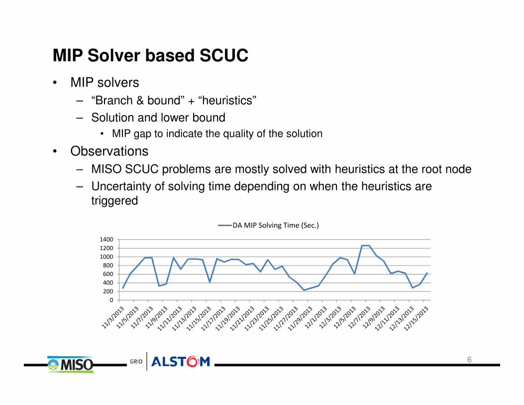
• Observations
– MISO SCUC problems are mostly solved with heuristics at the root node
– Uncertainty of solving time depending on when the heuristics are triggered
0
200
400
600
800
1000
1200
1400
DA MIP Solving Time (Sec.)
6
MIP Solver based SCUC (Cont.)
• Day-ahead case – Without transmission constraints, MISO DA cases can solve in ~100s
• Number of binaries is not the single contributor of performance challenge
– Transmission constraints and continuous virtual variables can cause very dense matrix and drive performance challenge
• DA SCUC requires longer time to solve with large number of continuous variables and dense matrix
– Longer time to solve root relaxation LP
– Longer time to solve each LP problem during the MIP searching process
• MIP may not solve faster even if it is fed with a better initial binary solution
• Uncertainty of solution quality at the time limit
• FRAC case– With no virtuals, the challenge is primarily driven by number of binaries
• Especially for 7-day FRAC cases under load increasing pattern, i.e. requiring more commitment for future days
– Primarily consider commitment cost with near zero incremental energy and reserve cost can cause the problem to be harder to solve
– Multi-thread and parameter tuning can help improve the performance
7
MIP Solver based SCUC (Cont.)
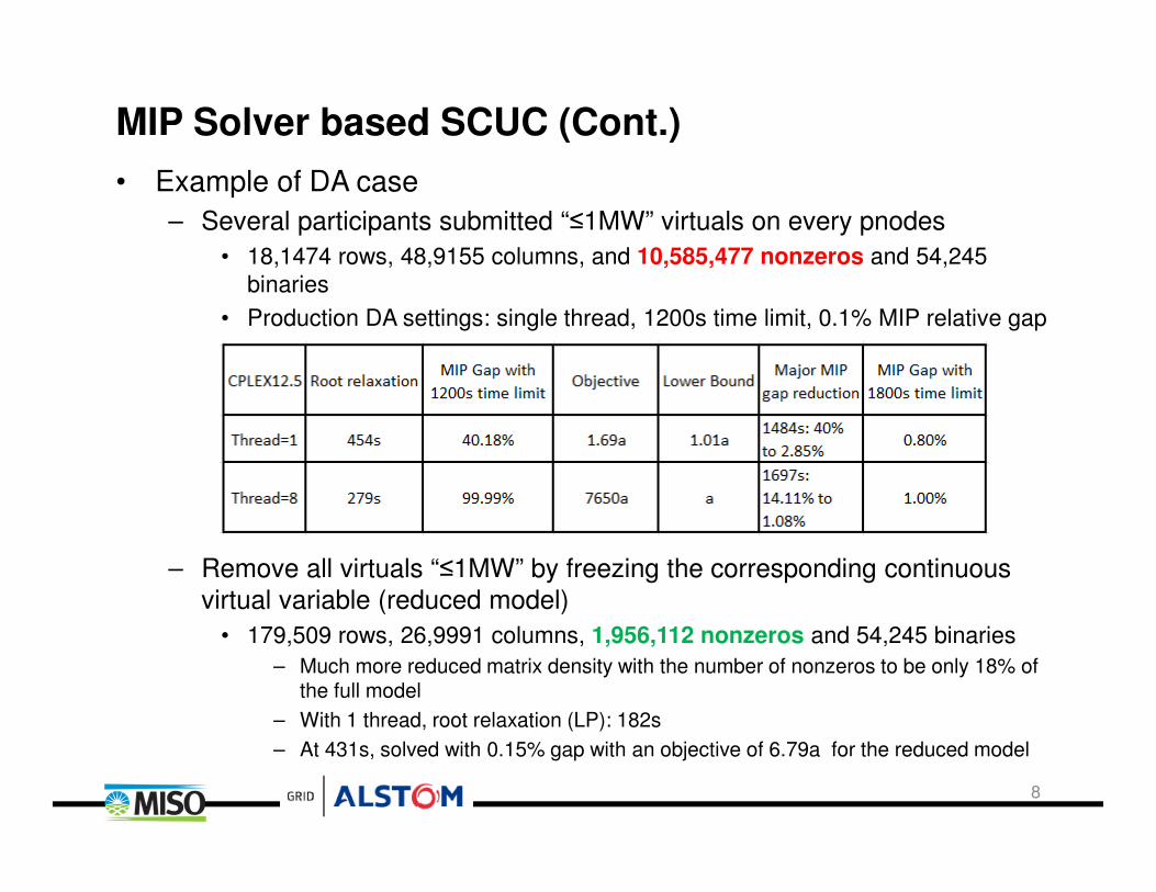
• Example of DA case
– Several participants submitted “≤1MW” virtuals on every pnodes
• 18,1474 rows, 48,9155 columns, and 10,585,477 nonzeros and 54,245 binaries
• Production DA settings: single thread, 1200s time limit, 0.1% MIP relative gap
– Remove all virtuals “≤1MW” by freezing the corresponding continuous virtual variable (reduced model)
• 179,509 rows, 26,9991 columns, 1,956,112 nonzeros and 54,245 binaries
– Much more reduced matrix density with the number of nonzeros to be only 18% of the full model
– With 1 thread, root relaxation (LP): 182s
– At 431s, solved with 0.15% gap with an objective of 6.79a for the reduced model
8
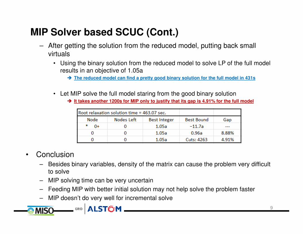
MIP Solver based SCUC (Cont.)
– After getting the solution from the reduced model, putting back small virtuals
• Using the binary solution from the reduced model to solve LP of the full modelresults in an objective of 1.05a
� The reduced model can find a pretty good binary solution for the full model in 431s
• Let MIP solve the full model staring from the good binary solution� It takes another 1200s for MIP only to justify that its gap is 4.91% for the full model
• Conclusion– Besides binary variables, density of the matrix can cause the problem very difficult
to solve
– MIP solving time can be very uncertain
– Feeding MIP with better initial solution may not help solve the problem faster
– MIP doesn’t do very well for incremental solve
9
Strategies for Improving the Performance
• Collaboration with Operations Research community to improve the MIP solver
– Existing MIP solvers cannot handle the DA problem caused by dense matrix very well. Have been working with the R&D experts on the solver side.
– So far there hasn’t been fundamental breakthrough
• MISO/Alstom collaboration to develop heuristics to improve SCUC performance
– LR based approach and decomposition based approach• Using MIP to solve sub-problems makes it much easier to implement the heuristic
approaches
– Fundamental issue: how to justify the optimality
• MISO/Alstom collaboration to improve the entire commitment solving process
– Improve the efficiency of DA-SCED, network analysis and software architecture• Phase I of the effort has reduced DA-SCED solving time by ~50%
• Continue the effort in 2014-2016
– Improve the capability of incremental solve• MIP cannot handle incremental solve very well
• R&D prototype to use LR based approach for incremental changes
10
Strategies for Improving the Performance (Cont.)
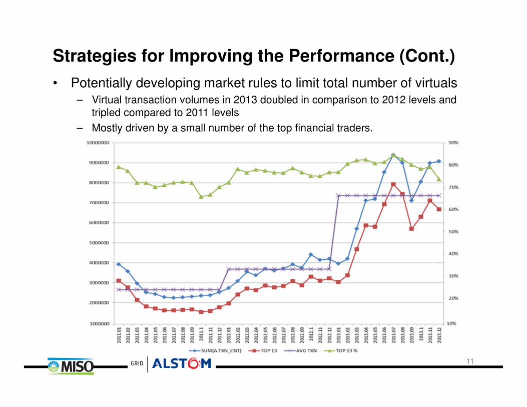
• Potentially developing market rules to limit total number of virtuals– Virtual transaction volumes in 2013 doubled in comparison to 2012 levels and
tripled compared to 2011 levels
– Mostly driven by a small number of the top financial traders.
11
Strategies for Improving the Performance (Cont.)
– Possible rules to limit total number of virtuals
• Impose administrative fees
• Limit number of virtual offers from each participant
• Hardware/OS options– Current server: HP DL380Gen 8 Server Chassis; 2 Intel Xeon E5-2690 8 core
CPUs; 64 GB memory
– MIP solvers need more time to solve dense cases. More powerful hardware can potentially help.
– Linux may give better performance over windows
12
Prototype Heuristic 1: LR Based Approach
• Incrementally adjust the commitment of a subset of the resources– Step 1: solve MIP with no transmission constraint (fast)
– Step 2: freeze commitment variables, add all transmission constraints and solve LP (fast)
– Step 3: Based on the prices, solve profit maximization for each resources (fast)
– Step 4: Compare the profit between step 2 and 3, select the top ~20 resources out of the money for commitment adjustment. Freeze commitment variables of all other resources. Solve MIP for the top ~20 resources. (200s~500s).
– Go to Step 3.
• This approach can also start from any other feasible solutions. Potential usage:– Backup approach to solve SCUC
– Solution polishing when MIP gap is relatively large
– Quickly solving commitment for increment changes
• Issue: no good indicator of the optimality gap
13
Prototype Heuristic 2: Decomposition Approach
• Handle transmission constraint incrementally– Step 1: solve MIP UC (i.e. master problem) with no transmission
constraint (fast)
– Step 2: freeze commitment variables, add all transmissions back to generate a LP (i.e. sub-problem). Solve this LP (fast)
– Step 3: Pick (severe) violated transmissions and feed them back into the master problem; re-optimize the MIP with additional transmission constraints (600s~700s)
– Step 4: Compare the objectives between Step 2 and Step 3. Stop the iteration if they are within the gap requirement
– Go to Step 2.
• Usually achieve a good feasible solution (<10% gap) after two iterations.
– Master problem grows with more transmission constraint after each iteration.
– Final master problem MIP gap reflects global optimality if the approach converges
– No good optimality gap indicator if the approach doesn’t converge well
14
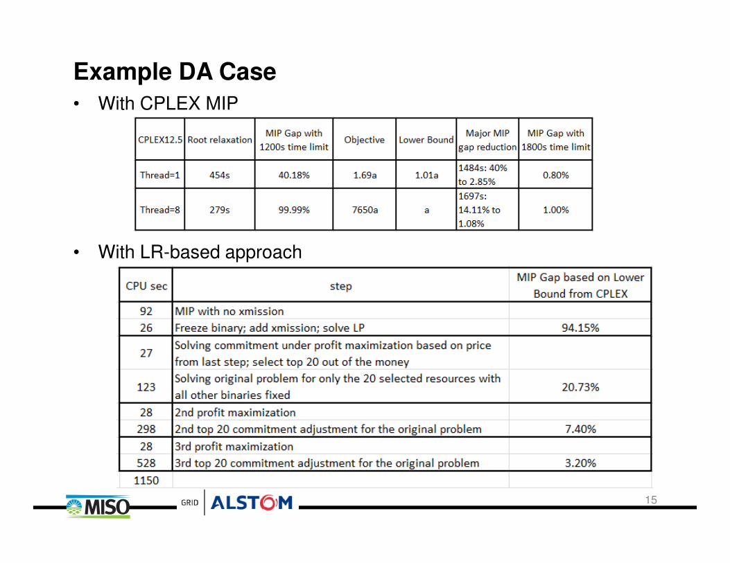
Example DA Case
• With CPLEX MIP
• With LR-based approach
15
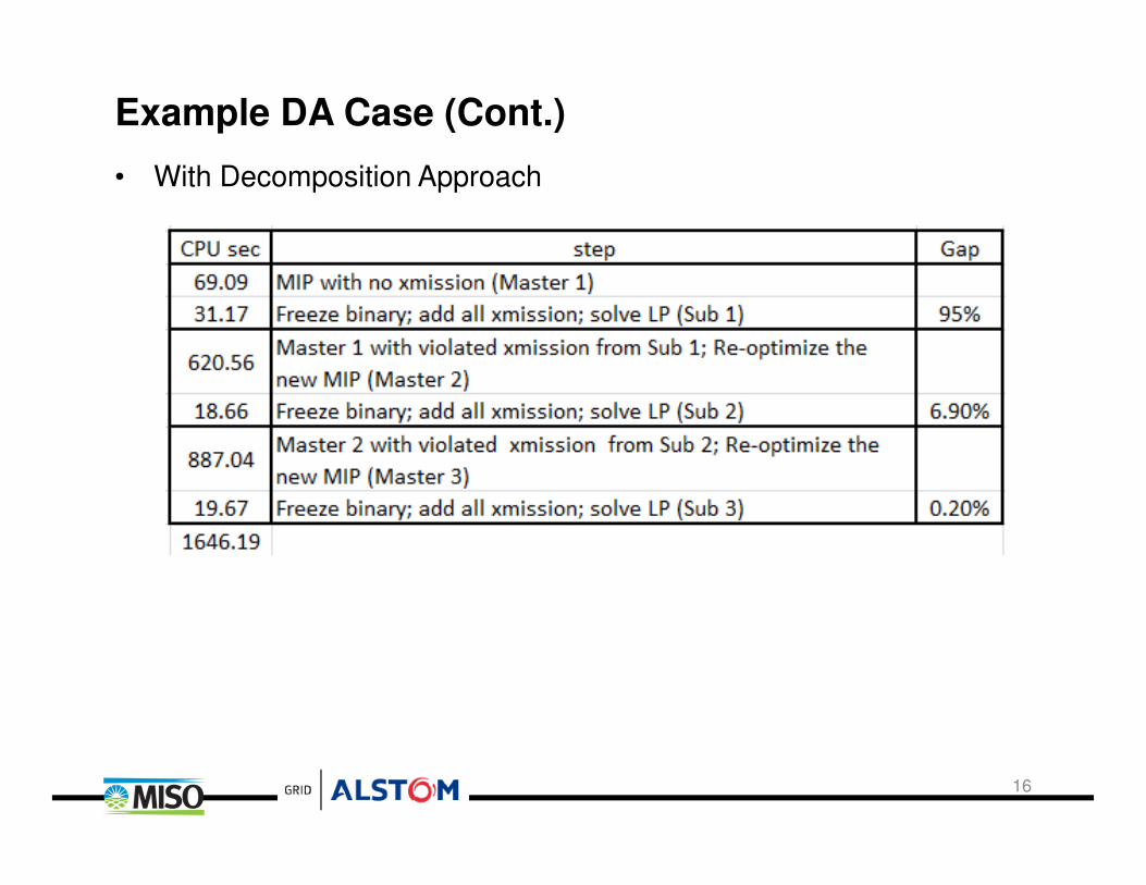
Example DA Case (Cont.)
• With Decomposition Approach
16
Improve the Capability of Incremental solve
• Operators need to make incremental solves every day– Add additional transmission constraints
– IMM mitigation on offers
– Determine commitment reasons for uplift cost allocation
• MIP cannot handle incremental solve very well– MIP may not solve faster even if it starts with a binary solution closer to
the optimal
• LR based approach may improve the incremental solve capability– Example: determine commitment reason
• Some “load pockets” in the south region requires using “N-2” limits while other parts of the system require “N-1” limits
• Need to determine the additional commitment for “N-2” for uplift allocation purpose
• Approach: compare commitment difference between “N-2” and “N-1”. For one DA case:
– Starting from “N-2” MIP solution, applying “N-1” limits and solve MIP: 1251s to reach 0.17% gap.
– Starting from “N-2” MIP solution, one iteration of LR based approach can reach 0.79% gap in 231s CPU time.
17
Next Steps for Improving Existing SCUC Performance
• Short term– Solver performance option tuning and upgrade– Use MIP solver as the primary approach to solve the full SCUC problem– Use “LR based Approach” or “Decomposition Approach” as the backup
approach – Improve the incremental solve capability and improve the entire commitment
process– MISO operations also monitor the number of virtual transactions and
request top traders to reduce the number of offers if needed
• Long term– Work with OR experts to
• Incorporate the heuristics into the solver• Develop other new approaches