177
July 2010 G. Moricca 1 Electric Submersible Pump Systems - 5 days course
| Date post: | 22-Jan-2018 |
| Category: |
Technology |
| Upload: | giuseppe-moricca |
| View: | 339 times |
| Download: | 11 times |

July 2010 G. Moricca 1
Electric Submersible
Pump Systems
-5 days course

July 2010 G. Moricca 2
Course agenda
Day 1
Overview of Artificial Lift Technology and
Introduction to ESP Systems
Day 2
ESP Basic Design and Operational Factors
Days 3
ESP System Components and their Operational Features
Day 4
ESP System design: step-by-step procedure
Day 5
ESP Installation Monitoring, Optimization, Troubleshooting and Diagnostic
July 2010 G. Moricca 3
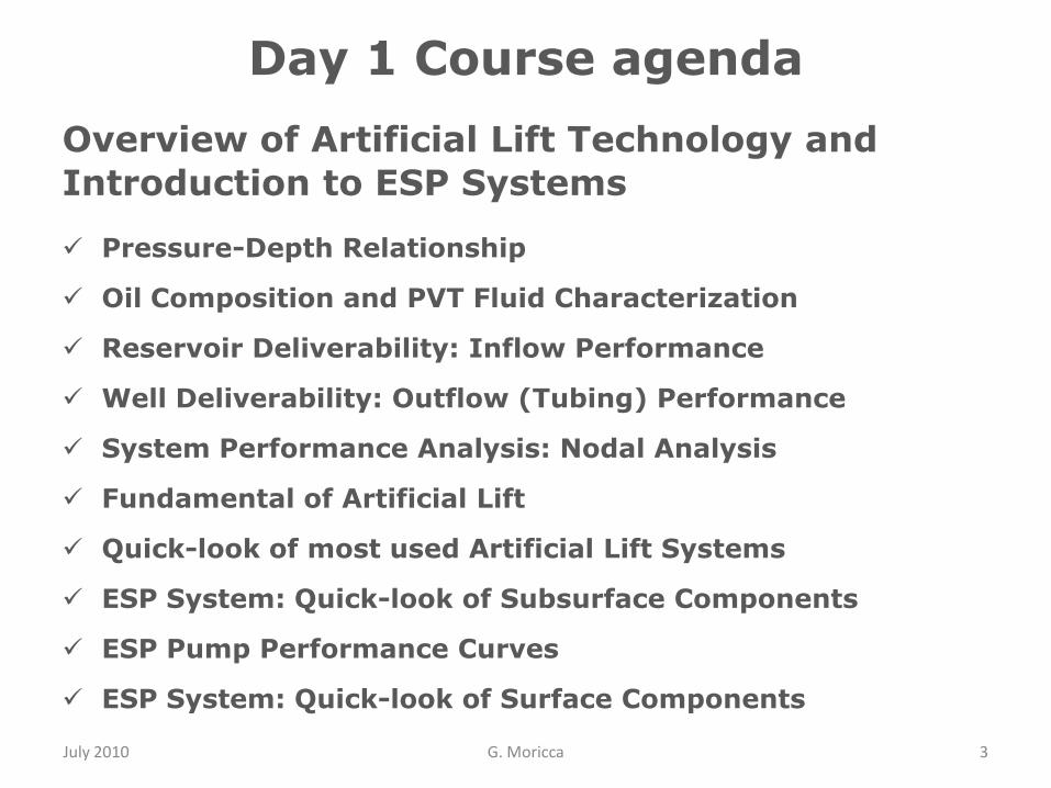
Day 1 Course agenda
Overview of Artificial Lift Technology and
Introduction to ESP Systems
Pressure-Depth Relationship
Oil Composition and PVT Fluid Characterization
Reservoir Deliverability: Inflow Performance
Well Deliverability: Outflow (Tubing) Performance
System Performance Analysis: Nodal Analysis
Fundamental of Artificial Lift
Quick-look of most used Artificial Lift Systems
ESP System: Quick-look of Subsurface Components
ESP Pump Performance Curves
ESP System: Quick-look of Surface Components
July 2010 G. Moricca 4
Pressure-Depth
Relationship
Main sources: Well Completion Design. Jonathan Bellarby. Elsevier Inc

July 2010 G. Moricca 5
Pressure-Depth Relationship
At the end of this section, you will be able to…
● Calculate Fluid Gradient given Density
● Calculate the Pressure given Depth and Gradient or Density
● Calculate the equivalent Fluid column when given pressure
and gradient or Density
● Calculate the fluid gradient when given the pressure
differential and the Depth
● Estimate Fluid level or surface pressure when given
pressure at depth and fluid gradient
● Draw a simple pressure-depth plot.
July 2010 G. Moricca 6
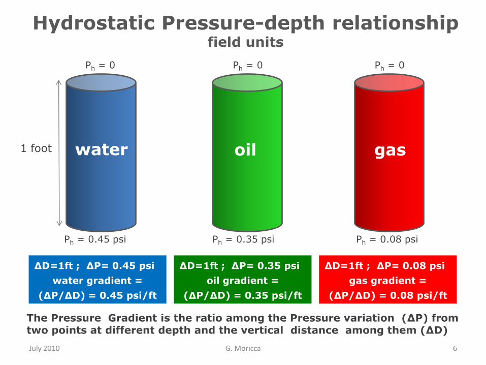
Hydrostatic Pressure-depth relationshipfield units
ΔD=1ft ; ΔP= 0.45 psi
water gradient =
(ΔP/ΔD) = 0.45 psi/ft
ΔD=1ft ; ΔP= 0.35 psi
oil gradient =
(ΔP/ΔD) = 0.35 psi/ft
ΔD=1ft ; ΔP= 0.08 psi
gas gradient =
(ΔP/ΔD) = 0.08 psi/ft
The Pressure Gradient is the ratio among the Pressure variation (ΔP) from two points at different depth and the vertical distance among them (ΔD)
1 foot water oil gas
Ph = 0.45 psi Ph = 0.08 psiPh = 0.35 psi
Ph = 0 Ph = 0Ph = 0
July 2010 G. Moricca 7
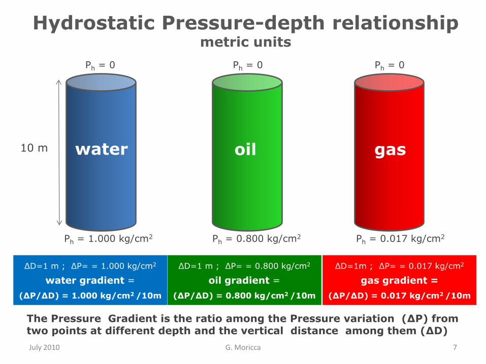
Hydrostatic Pressure-depth relationshipmetric units
ΔD=1 m ; ΔP= = 1.000 kg/cm2
water gradient =
(ΔP/ΔD) = 1.000 kg/cm2 /10m
ΔD=1 m ; ΔP= = 0.800 kg/cm2
oil gradient =
(ΔP/ΔD) = 0.800 kg/cm2 /10m
ΔD=1m ; ΔP= = 0.017 kg/cm2
gas gradient =
(ΔP/ΔD) = 0.017 kg/cm2 /10m
The Pressure Gradient is the ratio among the Pressure variation (ΔP) from two points at different depth and the vertical distance among them (ΔD)
10 m water oil gas
Ph = 1.000 kg/cm2 Ph = 0.017 kg/cm2Ph = 0.800 kg/cm2
Ph = 0 Ph = 0Ph = 0
July 2010 G. Moricca 8
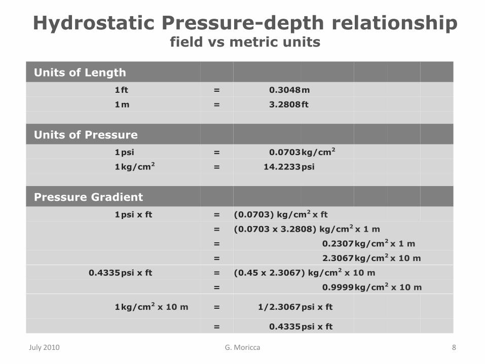
Hydrostatic Pressure-depth relationshipfield vs metric units
Units of Length
1ft = 0.3048m
1m = 3.2808ft
Units of Pressure
1psi = 0.0703kg/cm2
1kg/cm2 = 14.2233psi
Pressure Gradient
1psi x ft = (0.0703) kg/cm2 x ft
= (0.0703 x 3.2808) kg/cm2 x 1 m
= 0.2307kg/cm2 x 1 m
= 2.3067kg/cm2 x 10 m
0.4335psi x ft = (0.45 x 2.3067) kg/cm2 x 10 m
= 0.9999kg/cm2 x 10 m
1kg/cm2 x 10 m = 1/2.3067psi x ft
= 0.4335psi x ft
July 2010 G. Moricca 9
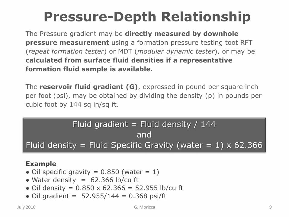
Pressure-Depth RelationshipThe Pressure gradient may be directly measured by downhole
pressure measurement using a formation pressure testing toot RFT
(repeat formation tester) or MDT (modular dynamic tester), or may be
calculated from surface fluid densities if a representative
formation fluid sample is available.
The reservoir fluid gradient (G), expressed in pound per square inch
per foot (psi), may be obtained by dividing the density (ρ) in pounds per
cubic foot by 144 sq in/sq ft.
Example
● Oil specific gravity = 0.850 (water = 1)
● Water density = 62.366 lb/cu ft
● Oil density = 0.850 x 62.366 = 52.955 lb/cu ft
● Oil gradient = 52.955/144 = 0.368 psi/ft
Fluid gradient = Fluid density / 144
and
Fluid density = Fluid Specific Gravity (water = 1) x 62.366

Calculating Pressure Gradient of Producing fluid
Data
● Producing fluid:
― Oil 25 API
― Water Cut (WC) = 80 %
― Formation water Specific Gravity = 1.04
● Density of pure water = 62.3 lb/cu ft
● Specific Gravity of pure water = 1
Calculate Pressure Gradient of Producing fluid
Solution
● Oil Specific Gravity = 141.5 / (131.5 + 25) = 0.904
● Producing fluid Specific Gravity = (SGwater x WC) + [SGoil x (1–WC)]
= (1.04 x 0.8) + [0.904 x (1–0.8)] = 1.013
● Density of produced fluid = 1.013 x 62.3 = 63.1099 lb/cu ft
● Gradient of produced fluid = 63.1099/144 = 0.438 psi/ft
July 2010 10G. Moricca
Calculating Pressure Gradient of Producing fluid
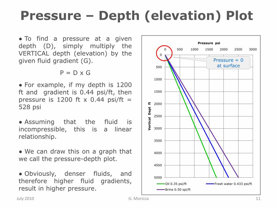
● To find a pressure at a givendepth (D), simply multiply theVERTICAL depth (elevation) by thegiven fluid gradient (G).
P = D x G
● For example, if my depth is 1200ft and gradient is 0.44 psi/ft, thenpressure is 1200 ft x 0.44 psi/ft =528 psi
● Assuming that the fluid isincompressible, this is a linearrelationship.
● We can draw this on a graph thatwe call the pressure-depth plot.
● Obviously, denser fluids, andtherefore higher fluid gradients,result in higher pressure.
0
500
1000
1500
2000
2500
3000
3500
4000
4500
5000
0 500 1000 1500 2000 2500 3000
Verti
cal D
ep
t f
t
Pressure psi
Oil 0.35 psi/ft Fresh water 0.433 psi/ft
Brine 0.50 spi/ft
Pressure = 0 at surface
July 2010 11G. Moricca
Pressure – Depth (elevation) Plot

Pressure – Depth (elevation) Plot
July 2010 G. Moricca 12
If the pressure at surface isn‟tzero, then the whole line shiftsover according to the surfacepressure.
If the lines maintain the same slope (they are parallel) this means that we are dealing with the same fluid.
Reservoir ASpecific Gravity Oil 0.809 (44°API)
Pore pressure gradient 0.35 spi/ft
Reservoir BSpecific Gravity Oil 0.809 (44°API)
Pore pressure gradient 0.40 spi/ft
Reservoir CSpecific Gravity Oil 0.809 (44°API)
Pore pressure gradient 0.45 spi/ft
B CA
0
500
1000
1500
2000
2500
3000
3500
4000
4500
5000
0 500 1000 1500 2000 2500
Verti
cal D
ep
t f
t
Pressure psi
Fluid Gradient 0,35 psi/ft
Pore Pressure Gradient 0.35 psi/ft
Pore Pressure Gradient 0.40 psi7ft
Pore pressure Gradient 0.45 psi/ft
Pressure – Depth (elevation) Plot
Pressure – Depth (elevation) Plot
July 2010 G. Moricca 13
0
500
1000
1500
2000
2500
3000
3500
4000
4500
5000
0 500 1000 1500 2000 2500 3000
Verti
cal D
ep
t f
t
Pressure psi
Fluid Gradient 0.35 psi/ft
Pore Pressure Gradient 0.28 psi/ft
Depleted Reservoir
Fliud Gradient 0.35 psi/ft
0
500
1000
1500
2000
2500
3000
3500
4000
4500
5000
0 500 1000 1500 2000 2500 3000
Verti
cal D
ep
t f
t
Pressure psi
Fluid Gradient 0.60 psi/ft
Pore Pressure Gradient 0.48 psi/ft
Killed well
Fliud Gradient 0.60 psi/ft
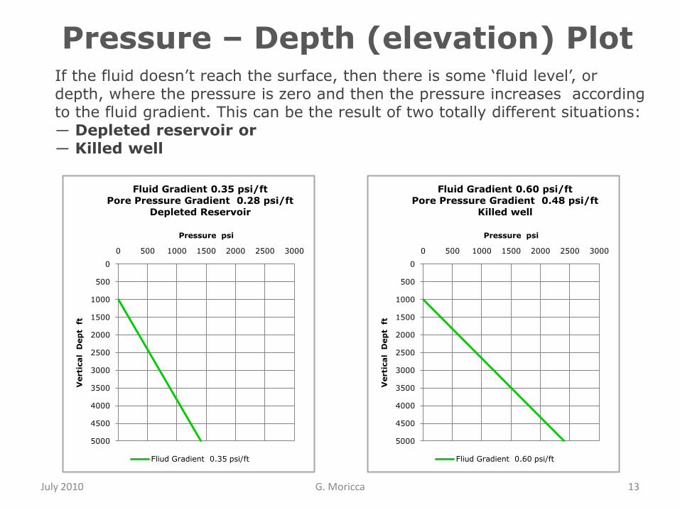
If the fluid doesn‟t reach the surface, then there is some „fluid level‟, or depth, where the pressure is zero and then the pressure increases according to the fluid gradient. This can be the result of two totally different situations:― Depleted reservoir or― Killed well
Pressure – Depth (elevation) Plot

Calculating the Fluid Height or Fluid Column
July 2010 G. Moricca 14
● Similarly, if we know thepressure and the fluid gradient,we can calculate the equivalentfluid column resulting from thatpressure:
H = P/G
―Measured pressure = 2500 psi―Fluid gradient = 0.25 psi/ft―Equivalent fluid column =
2500/0.25 = 10.000 ft
● Here the effect of increasinggradient is reversed, and adenser fluid results in a shorterfluid column for a given pressure.
● Because oil is lighter than water(responsible of “normal” or“hydrostatic” pressure regime),this is the reason that oil wellsflow naturally !
0
1000
2000
3000
4000
5000
6000
7000
8000
9000
10000
11000
12000
13000
0 500 1000 1500 2000 2500 3000
Eq
uiv
ale
t fl
uid
co
lum
n ft
Pressure psi
Fliud Gradient 0.20 psi/ft
Fluid Gradient 0.30 psi/ft
Fluid Gradient 0.40 psi/ft
Fluid Gradient 0.5 psi/ft
Fluid Gradient 0.6 psi/ft
Calculating the Fluid Height or Fluid Column

Normal and Abnormal Pressure Regimes
July 2010 G. Moricca 15
In abnormally pressured reservoir, the continuous pressure-dept relationship is interrupted by a sealing layer, below which the pressure change. In order to maintain underpressure or overpressure, a pressure seal must be present. In hydrocarbon reservoir, there is by definition a seal at the creastof the accumulation, and potential for abnormal pressure regimes therefore exists. The most common causes of abnormally pressured reservoirs are:
Uplift/burial of rock
Thermal effects, causing the expansion or contraction of water
Depletion of a sealed or low-permeability reservoir due to production within the reservoir
Depletion due to production in an adjacent field
Normal and Abnormal Pressure Regimes

Normal Pressure Distribution from Surface through a Reservoir Structure
July 2010 G. Moricca 16
In the water column, the pressure at any depth can be approximated to:
P = D x Gw
where: D is the vertical depth and Gw is the pressure gradient
P = D x Gw
D = 5000 ft
Gw = 0.45 spi/ft
P = 5000 x 0.45 =
2250 psi
Normal Pressure Distribution from Surface through a Reservoir Structure
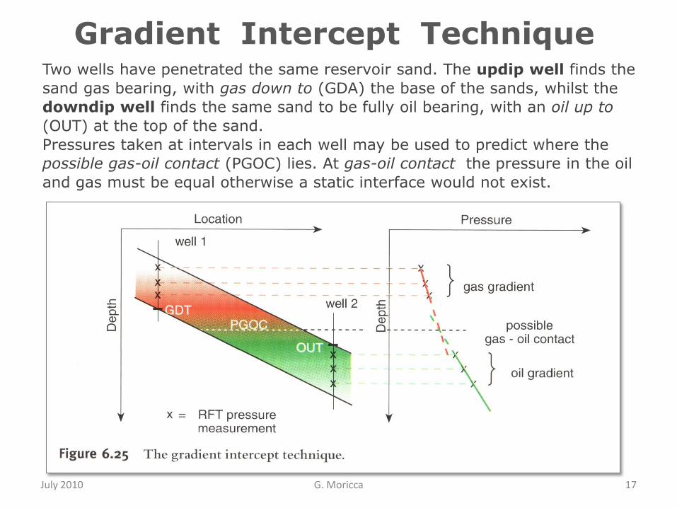
Gradient Intercept Technique
July 2010 G. Moricca 17
Two wells have penetrated the same reservoir sand. The updip well finds the
sand gas bearing, with gas down to (GDA) the base of the sands, whilst the
downdip well finds the same sand to be fully oil bearing, with an oil up to
(OUT) at the top of the sand.
Pressures taken at intervals in each well may be used to predict where the
possible gas-oil contact (PGOC) lies. At gas-oil contact the pressure in the oil
and gas must be equal otherwise a static interface would not exist.
Gradient Intercept Technique
July 2010 G. Moricca 18
Oil Composition
and
PVT Fluid
Characterization
Main source: Fundamentals of Reservoir Engineering. L. P. Dake. Elsevier Inc
July 2010 G. Moricca 19
At the end of this section, you will be able to
understand the…
● Hydrocarbon Phase Behaviour
● PVT parameters required to relate surface to reservoir
volumes for an oil reservoir
and…
● Calculate the PVT parameters through Empirical Correlations
● Estimate the PVT Properties from Production Data
Reservoir Fluids Characterisation

Reservoir Fluids Characterisation
July 2010 G. Moricca 20
Reservoir fluids are broadly categorised using those properties which are easy to measure, namely oil and gas gravity and producing GOR.
Reservoir Fluids Characterisation
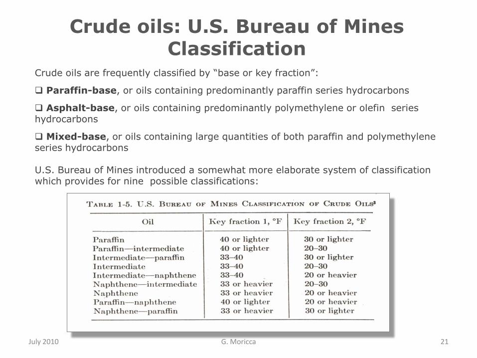
Crude oils: U.S. Bureau of Mines Classification
July 2010 G. Moricca 21
Crude oils are frequently classified by “base or key fraction”:
Paraffin-base, or oils containing predominantly paraffin series hydrocarbons
Asphalt-base, or oils containing predominantly polymethylene or olefin series hydrocarbons
Mixed-base, or oils containing large quantities of both paraffin and polymethyleneseries hydrocarbons
U.S. Bureau of Mines introduced a somewhat more elaborate system of classification which provides for nine possible classifications:
Crude oils: U.S. Bureau of Mines Classification

Crude oils Commercial Classification
July 2010 G. Moricca 22
West Texas Intermediate (WTI), a very high-quality, sweet, light oil delivered at Cushing, Oklahoma for North American oil
Brent Blend, comprising 15 oils from fields in the Brent and Niniansystems in the East Shetland Basin of the North Sea.
Dubai-Oman, used as benchmark for Middle East sour crude oil flowing to the Asia-Pacific region
Tapis (from Malaysia, used as a reference for light Far East oil)
Minas (from Indonesia, used as a reference for heavy Far East oil)
The OPEC Reference Basket, a weighted average of oil blends from various OPEC
The petroleum industry generally classifies crude oil by the geographic location it is produced in (e.g. West Texas Intermediate, Brent, or Oman), its API gravity and by its sulfur content. Crude oil may be considered light if it has low density or heavy if it has high density; and it may be referred to as sweet if it contains relatively little sulfur or sour if it contains substantial amounts of sulfur.
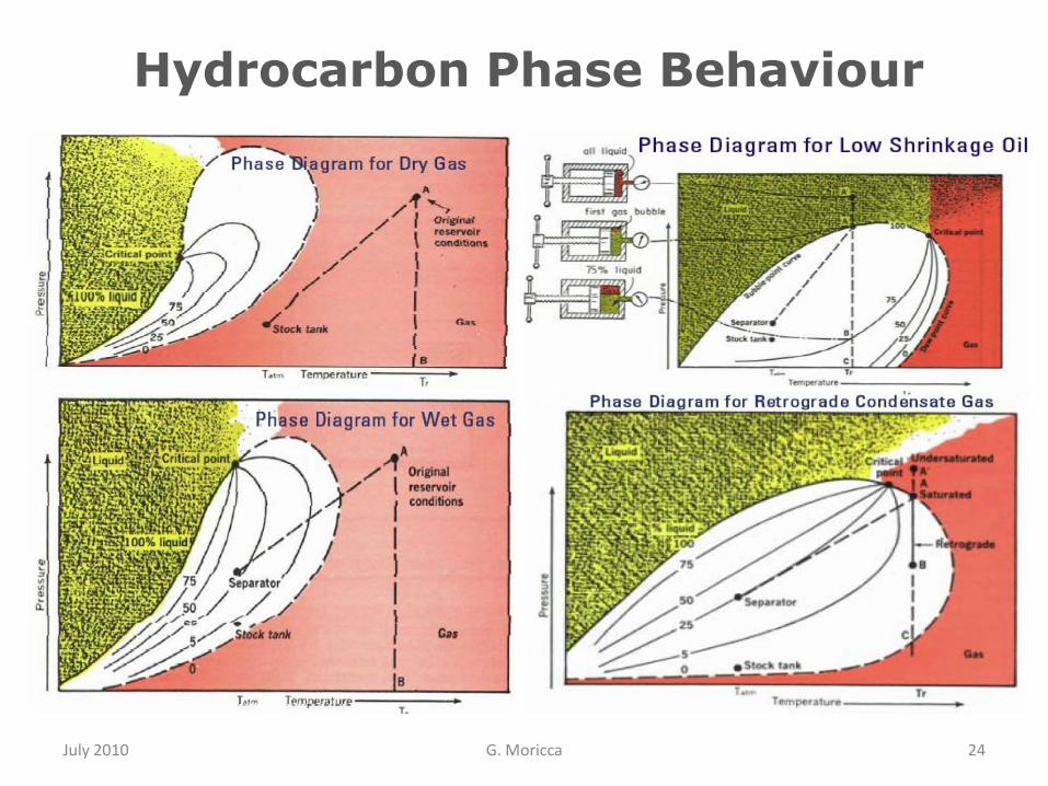
Hydrocarbon Phase Behaviour
July 2010 G. Moricca 23
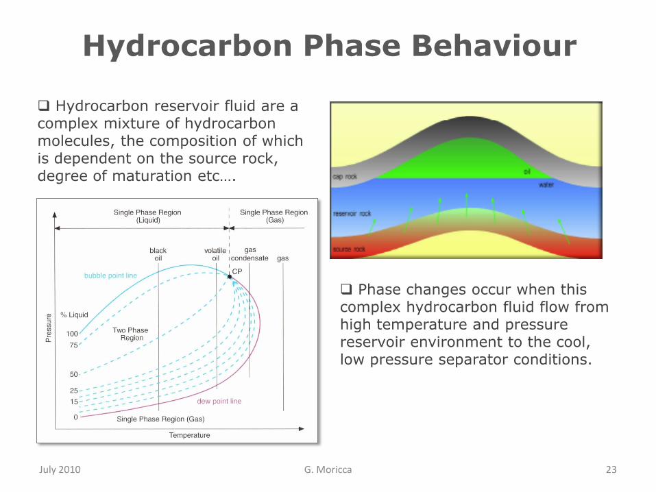
Hydrocarbon reservoir fluid are acomplex mixture of hydrocarbonmolecules, the composition of which is dependent on the source rock, degree of maturation etc….
Phase changes occur when thiscomplex hydrocarbon fluid flow fromhigh temperature and pressure reservoir environment to the cool, low pressure separator conditions.
Hydrocarbon Phase Behaviour
July 2010 G. Moricca 24
Crude Oil Characteristics
July 2010 G. Moricca 25
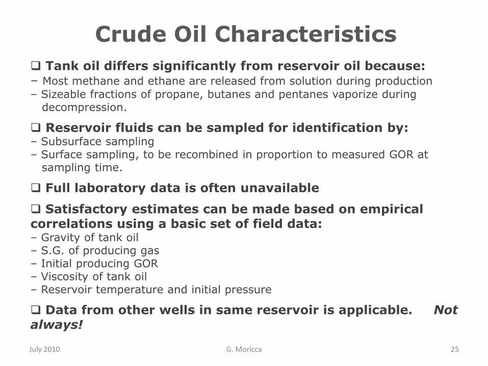
Tank oil differs significantly from reservoir oil because:– Most methane and ethane are released from solution during production
– Sizeable fractions of propane, butanes and pentanes vaporize duringdecompression.
Reservoir fluids can be sampled for identification by:– Subsurface sampling– Surface sampling, to be recombined in proportion to measured GOR at
sampling time.
Full laboratory data is often unavailable
Satisfactory estimates can be made based on empirical correlations using a basic set of field data:– Gravity of tank oil– S.G. of producing gas– Initial producing GOR– Viscosity of tank oil– Reservoir temperature and initial pressure
Data from other wells in same reservoir is applicable. Not always!
Crude Oil PVT Behaviour
July 2010 G. Moricca 26
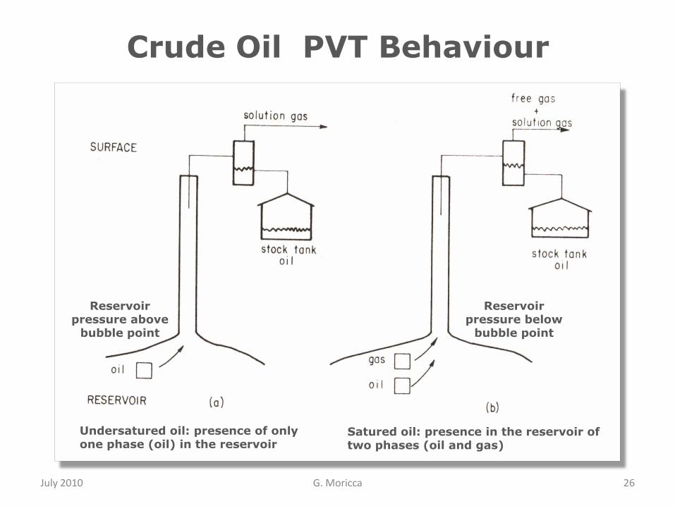
Undersatured oil: presence of only one phase (oil) in the reservoir
Satured oil: presence in the reservoir of two phases (oil and gas)
Reservoir pressure above
bubble point
Reservoir pressure below
bubble point
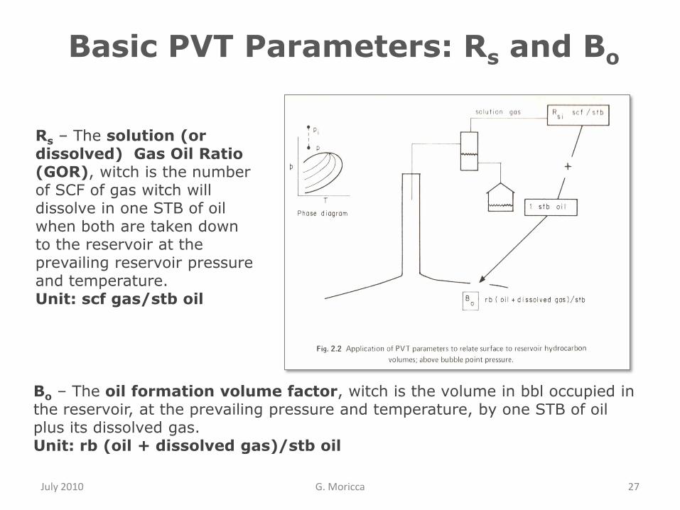
Basic PVT Parameters: Rs and Bo
July 2010 G. Moricca 27
Rs – The solution (or dissolved) Gas Oil Ratio (GOR), witch is the number of SCF of gas witch will dissolve in one STB of oil when both are taken down to the reservoir at the prevailing reservoir pressure and temperature.Unit: scf gas/stb oil
Bo – The oil formation volume factor, witch is the volume in bbl occupied in the reservoir, at the prevailing pressure and temperature, by one STB of oil plus its dissolved gas. Unit: rb (oil + dissolved gas)/stb oil

Basic PVT Parameters: R and Bg
July 2010 G. Moricca 28
R – Instantaneous or producing Gas Oil Ratio (GOR) Unit: scf/stb
Bg – The gas formation volume factor, witch is the volume in bbl that one standard cubic foot of gas will occupy as free gas in the reservoir at the prevailing pressure and temperature. Unit: rb (free gas)/scf gas
Rs – The solution (or dissolved) Gas Oil Ratio (GOR), witch is the number of SCF of gas witch will dissolve in one STB of oil when both are taken down to the reservoir at the prevailing reservoir pressure and temperature.Unit: scf gas/stb oil
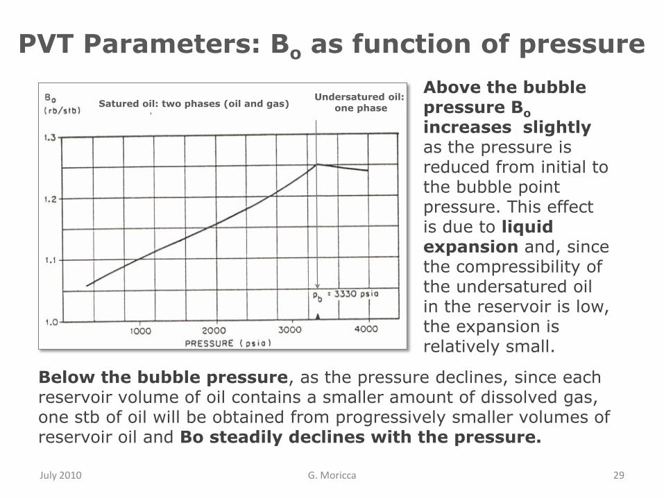
PVT Parameters: Bo as function of pressure
July 2010 G. Moricca 29
Above the bubble pressure Bo
increases slightly as the pressure is reduced from initial to the bubble point pressure. This effect is due to liquid expansion and, since the compressibility of the undersatured oil in the reservoir is low, the expansion is relatively small.
Undersatured oil:one phase Satured oil: two phases (oil and gas)
Below the bubble pressure, as the pressure declines, since each reservoir volume of oil contains a smaller amount of dissolved gas, one stb of oil will be obtained from progressively smaller volumes of reservoir oil and Bo steadily declines with the pressure.
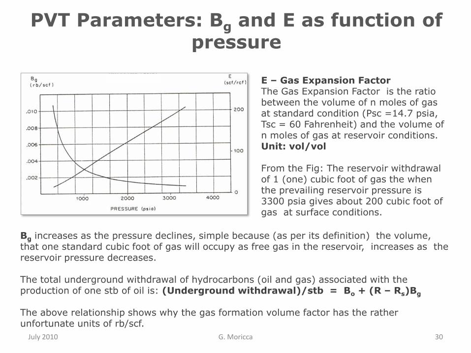
PVT Parameters: Bg and E as function of pressure
July 2010 G. Moricca 30
E – Gas Expansion FactorThe Gas Expansion Factor is the ratio between the volume of n moles of gas at standard condition (Psc =14.7 psia, Tsc = 60 Fahrenheit) and the volume of n moles of gas at reservoir conditions.Unit: vol/vol
From the Fig: The reservoir withdrawal of 1 (one) cubic foot of gas the when the prevailing reservoir pressure is 3300 psia gives about 200 cubic foot of gas at surface conditions.
Bg increases as the pressure declines, simple because (as per its definition) the volume, that one standard cubic foot of gas will occupy as free gas in the reservoir, increases as the reservoir pressure decreases.
The total underground withdrawal of hydrocarbons (oil and gas) associated with the production of one stb of oil is: (Underground withdrawal)/stb = Bo + (R – Rs)Bg
The above relationship shows why the gas formation volume factor has the rather unfortunate units of rb/scf.
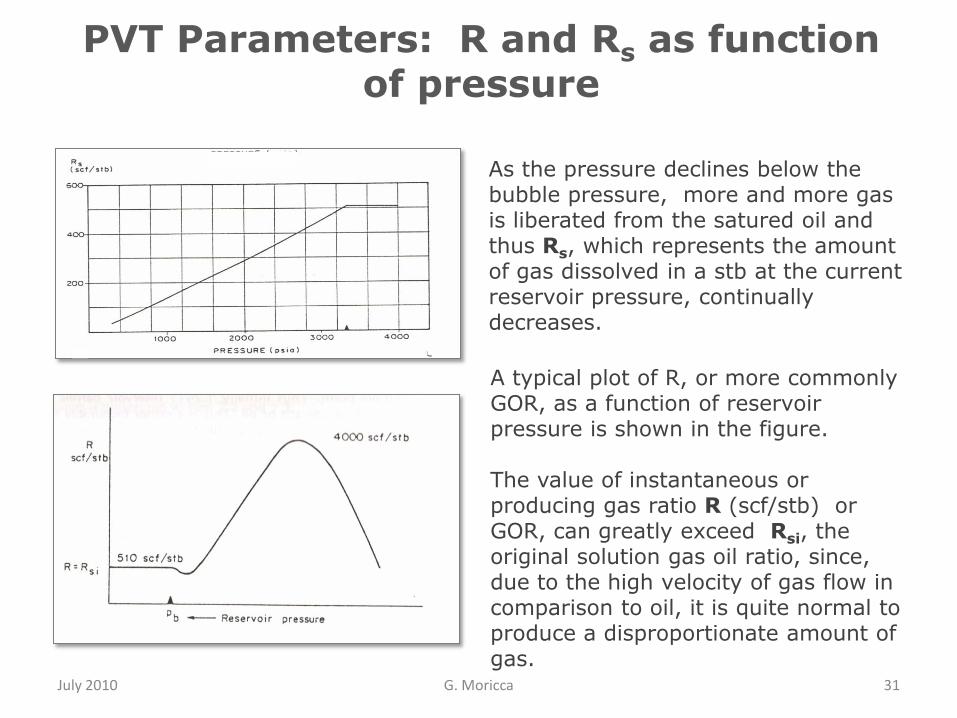
PVT Parameters: R and Rs as function of pressure
July 2010 G. Moricca 31
As the pressure declines below the bubble pressure, more and more gas is liberated from the satured oil and thus Rs, which represents the amount of gas dissolved in a stb at the current reservoir pressure, continually decreases.
A typical plot of R, or more commonly GOR, as a function of reservoir pressure is shown in the figure.
The value of instantaneous or producing gas ratio R (scf/stb) or GOR, can greatly exceed Rsi, the original solution gas oil ratio, since, due to the high velocity of gas flow in comparison to oil, it is quite normal to produce a disproportionate amount of gas.

PVT Empirical Correlations
July 2010 G. Moricca 32
BgGas Volume Factor : Volume in ft3 that one scf of gas will
occupy at specific P and T conditionft3/scf Bg = 0,02827 TZ/P
Bo
Oil Volume Factor : Volume in bbl occupied by one STB of oil
and its associated solution gas when recombined to a single-
phase liquid at specific P and T condition (Standing)
bbl/STB Bo = Bob exp [co (Pb - P)] ;
R < Rs unsatured oil
Bob Oil Volume Factor at Bubble-point pressure (Standing) bbl/STB Bob = 0,9759 + 12*10-5
Y1,2
; R > Rs satured oil
co Undersatured Oil Compresibility (Vazquez) 1/psi co = 10-5
[- 1433 +5 Rs + 17,2T - 1180γg + 12,61γAPI ] / P
Eg Fraction of the total area occupied by gas dimensionless Eg = (1 -EL)
EL Fraction of the total area occupied by liquid (Liquid holdup) dimensionless EL = 5,645 Bo / [(R - Rs)Bg + 5,615(Bo + Bw Fwo)]
Pb Bubble-point Presure (Standing) psi Pb = 18,2 (W - 1,4)
Rs
Solution Gas/Oil Ratio : Volume of gas (in scf) going into
solution in one STB of oil at given P and T conditions. Rs is the
total volume of gas collected from all stages of separation,
divided the volume of stock-tank oil (case of undersaturated oil
production). Rs is function of P and T (Standing)
scf/STB Rs = γg (1,4 + P/18,2)1,205
10 (0,0151γAPI - 0,0011T)
W Constant W = ( Rs / γg )0,83
10 (0,00091 T - 0,0125 γAPI )
Y Constant Y = 1,25 T + Rs [γg / γo ]1/2
ρL Liquid density lbm/ft3 ρL = [62,4 (γSTO + γw Fwo) + 0,0136 γg R] / (Bo + Bw Fwo)
ρm Mixture (oil water and gas) density lbm/ft3 ρm = ρL EL + ρm (1-EL)
ρm Mixture (oil water and gas) density lbm/ft4 ρm = [62,4 (γSTO + γw Fwo) + 0,0136 γg R] / [Bo + Bw Fwo + (R - Rs)Bg / 5,615
ρo Oil density lbm/ft3 ρo = [62,4 γSTO + 0,0136 γg Rs] / Bo
ρw Water density lbm/ft3 ρw = 62,4 γw / Bw
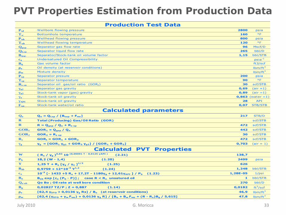
PVT Properties Estimation from Production Data
July 2010 G. Moricca 33
Pwf Wellbore flowing pressure 2800 psia
Tw Bottomhole temperature 160 °F
Pwh Wellhead flowing pressure 800 psia
Twh Wellhead flowing temperature 120 °F
Qgsp Separator gas flow rate 96 Mscf/D
QLsp Separator liquid flow rate 265 bbl/D
Bosp Separator/Stock-tank oil volume factor 1,15 bbl/STB
co Undersatured Oil Compressibility psia-1
Bg Gas volume factor ft3/scf
ρo Oil density (at reservoir conditions) lbm/ft3
ρm Mixture density lbm/ft3
Psp Separator presure 200 psia
Tsp Separator temperature 90 °F
Rs sp Separator oil gas/oil ratio (GOR2) 30 scf/STB
γg1 Separator gas gravity 0,69 (air =1)
γg2 Stock-tank vapor (gas) gravity 0,89 (air =1)
γo Stock-tank oil gravity 0,863 (water =1)
γAPI Stock-tank oil gravity 28 API
Fwo Stock-tank water/oil ratio 0,07 STB/STB
Qo Qo = QLsp / [Bosp + Fwo] 217 STB/D
R Total (Producing) Gas/Oil Ratio (GOR) scf/STB
R R = Qgsp / Qo + Rs sp 472 scf/STB
GOR1 GOR1 = Qgsp / Qo 442 scf/STB
GOR2 GOR2 = Rs sp 30 scf/STB
Rs GORt = GOR1 + GOR2 472 scf/STB
γg γg = [GOR1 γg1 + GOR2 γg2] / [GOR1 + GOR2] 0,703 (air = 1)
W ( Rs / γg )0,83
10 (0,00091 T - 0,0125 γAPI )
(2.21) 138,7
Pb 18,2 (W - 1,4) (1.20) 2499 psia
Y 1,25 T + Rs [γg / γo ]1/2
(1.25) 626
Bob 0,9759 + 12*10-5
Y1,2
(1.24) 1,248 bbl/STB
co 10-5
[- 1433 +5 Rs + 17,2T - 1180γg + 12,61γAPI ] / Pb (1.23) 1,28E-05 1/psi
Bo Bob exp [co (Pb - P)] ;
case R < Rs unsatured oil 1 bbl/STB
Qo wb Qo Bo ; Oil rate at well bore condition 270 bbl/D
Bg 0,02827 TZ/P ; Z = 0,887 (1.14) 0,0182 ft3/scf
ρo [62,4 γSTO + 0,0136 γg Rs] / Bo (at reservoir conditions) 46,9 lbm/ft3
ρm [62,4 (γSTO + γw Fwo) + 0,0136 γg R] / [Bo + Bw Fwo + (R - Rs)Bg / 5,615] 47,8 lbm/ft3
Calculated PVT Properties
Production Test Data
Calculated parameters

Oil Gravity Conversion
July 2010 G. Moricca 34
API 15 16 17 18 19 20 21 22 23 24 25 26 27 28 29 30
kg/l 0,966 0,959 0,953 0,946 0,940 0,934 0,928 0,922 0,916 0,910 0,904 0,898 0,893 0,887 0,882 0,876
API 31 32 33 34 35 36 37 38 39 40 41 42 43 44 45 50
kg/l 0,871 0,865 0,860 0,855 0,850 0,845 0,840 0,835 0,830 0,825 0,820 0,816 0,811 0,806 0,802 0,780
kg/l 0,990 0,985 0,980 0,975 0,970 0,965 0,960 0,955 0,950 0,945 0,940 0,935 0,930 0,925 0,920 0,915
API 11,4 12,2 12,9 13,6 14,4 15,1 15,9 16,7 17,4 18,2 19,0 19,8 20,7 21,5 22,3 23,1
kg/l 0,910 0,905 0,900 0,895 0,890 0,885 0,880 0,875 0,870 0,865 0,860 0,855 0,850 0,845 0,840 0,800
API 24,0 24,9 25,7 26,6 27,5 28,4 29,3 30,2 31,1 32,1 33,0 34,0 35,0 36,0 37,0 45,4
γo = 141,5 / (131,5 + γAPI )
γAPI = (141,5 / γo) - 131,5

July 2010 G. Moricca 35
ReservoirDeliverability:
Inflow Performance-
Pseudo-Steady-State Flow
Productivity Index
Vogel’s equation
Main source: Well Performance . M. Golan /C. H. Whitson. Prentice Hall Inc
July 2010 G. Moricca 36
Reservoir deliverability
At the end of this section, you will be able to…
● Calculate Outflow Pressure/Fluid Rate for a given set of
conditions using:
― Pseudo-Steady-State Flow
― Productivity Index
― Vogel‟s equation
● Calculate the absolute open flow (AOF)
● Generate an Inflow Performance Relationship (IPR)

Reservoir deliverability
July 2010 G. Moricca 37
Reservoir deliverability is defined as the oil or gas production rate achievable from reservoir at a given bottom-hole pressure.
Reservoir deliverability depend on several factors including the following:
● Reservoir pressure● Pay zone thickness and permeability● Reservoir boundary type and distance● Well radius● Reservoir fluid properties● Near well bare condition● Reservoir relative permeability
Symbolsp = average reservoir pressure, psiapwf = flowing bottom-hole pressure, psiaq = oil production rate, stb/dayµo = viscosity of oil, cpk = effective horizontal permeability to oil, mDh = reservoir thickness, ftr = reservoir boundary radius, ftrw = wellbore radius to the sand face, ftS = skin factor
Reservoir deliverability
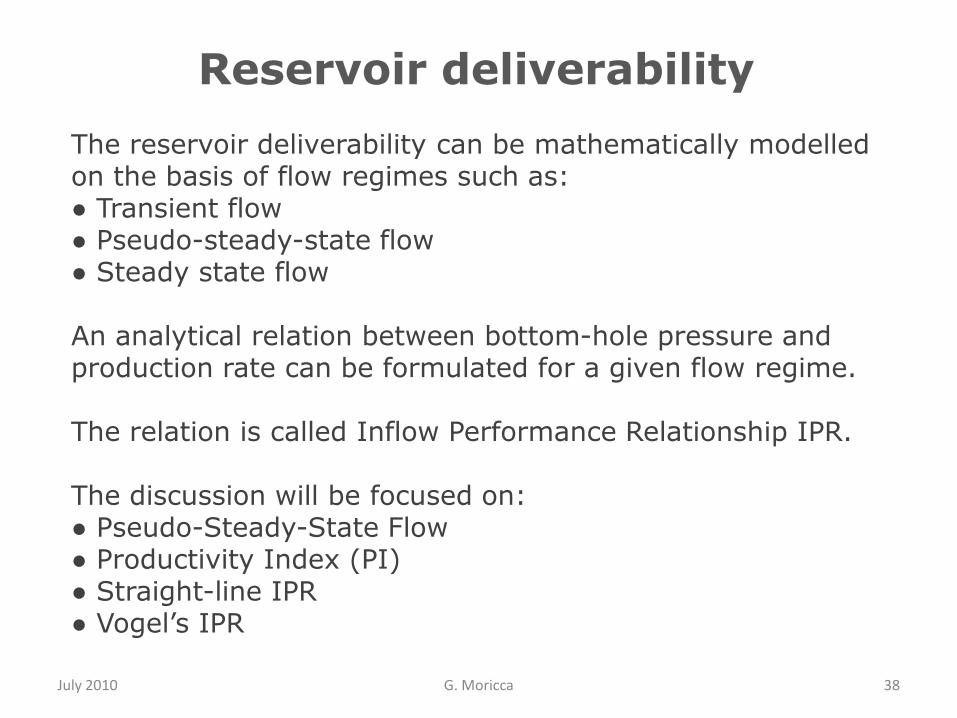
July 2010 G. Moricca 38
The reservoir deliverability can be mathematically modelled on the basis of flow regimes such as:● Transient flow● Pseudo-steady-state flow● Steady state flow
An analytical relation between bottom-hole pressure and production rate can be formulated for a given flow regime.
The relation is called Inflow Performance Relationship IPR.
The discussion will be focused on:● Pseudo-Steady-State Flow● Productivity Index (PI)● Straight-line IPR● Vogel‟s IPR
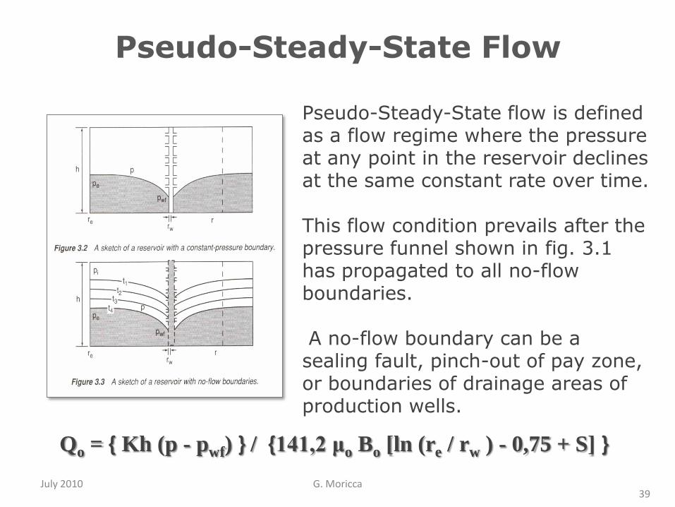
Pseudo-Steady-State Flow
July 2010 G. Moricca39
Pseudo-Steady-State flow is defined as a flow regime where the pressure at any point in the reservoir declines at the same constant rate over time.
This flow condition prevails after the pressure funnel shown in fig. 3.1 has propagated to all no-flow boundaries.
A no-flow boundary can be a sealing fault, pinch-out of pay zone, or boundaries of drainage areas of production wells.
Qo = { Kh (p - pwf) } / {141,2 μo Bo [ln (re / rw ) - 0,75 + S] }
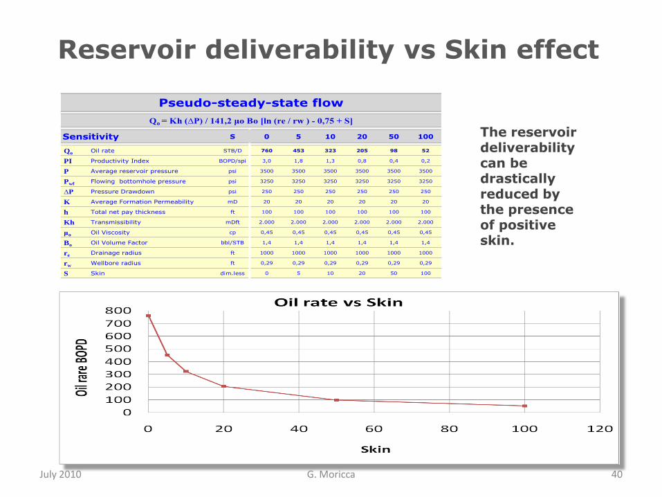
Reservoir deliverability vs Skin effect
July 2010 G. Moricca 40
The reservoir deliverability can be drastically reduced by the presence of positive skin.
S 0 5 10 20 50 100
Qo Oil rate STB/D 760 453 323 205 98 52
PI Productivity Index BOPD/spi 3,0 1,8 1,3 0,8 0,4 0,2
P Average reservoir pressure psi 3500 3500 3500 3500 3500 3500
Pwf Flowing bottomhole pressure psi 3250 3250 3250 3250 3250 3250
∆P Pressure Drawdown psi 250 250 250 250 250 250
K Average Formation Permeability mD 20 20 20 20 20 20
h Total net pay thickness ft 100 100 100 100 100 100
Kh Transmissibility mDft 2.000 2.000 2.000 2.000 2.000 2.000
μo Oil Viscosity cp 0,45 0,45 0,45 0,45 0,45 0,45
Bo Oil Volume Factor bbl/STB 1,4 1,4 1,4 1,4 1,4 1,4
re Drainage radius ft 1000 1000 1000 1000 1000 1000
rw Wellbore radius ft 0,29 0,29 0,29 0,29 0,29 0,29
S Skin dim.less 0 5 10 20 50 100
Pseudo-steady-state flow
Qo = Kh (∆P) / 141,2 μo Bo [ln (re / rw ) - 0,75 + S]
Sensitivity
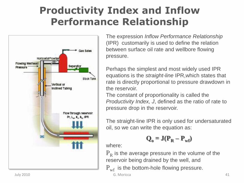
Productivity Index and Inflow Performance Relationship
July 2010 G. Moricca 41
The expression Inflow Performance Relationship
(IPR) customarily is used to define the relation
between surface oil rate and wellbore flowing
pressure.
Perhaps the simplest and most widely used IPR
equations is the straight-line IPR,which states that
rate is directly proportional to pressure drawdown in
the reservoir.
The constant of proportionality is called the
Productivity Index, J, defined as the ratio of rate to
pressure drop in the reservoir.
The straight-line IPR is only used for undersaturated
oil, so we can write the equation as:
Qo = J(PR – Pwf)where:
PR is the average pressure in the volume of the
reservoir being drained by the well, and
Pwf is the bottom-hole flowing pressure.
Productivity Index
July 2010 G. Moricca 42
Productivity Index: J = Qo / (PR – Pwf)
Oil rate: Qo = J(PR – Pwf)
Pressure Drawdown: ΔP = (PR – Pwf)
● By convention, the dependent variable rate defines the x axis and the independent
variable, wellbore flowing pressure, defines the y axis.
● When wellbore flowing pressure equals average reservoir pressure (sometimes
referred to as static pressure), rate is zero and no flow enters the wellbore due to the
absence of any pressure drawdown.
● Maximum rate of flow , Qmax, or absolute open flow, AOF, corresponds to wellbore
flowing pressure equal to zero.
● The slope of straight line equals the reciprocal of the productivity index (slope = 1/J).

Example: Straight line IPR Calculation
July 2010 G. Moricca 43
ProblemThe well Lamar 1 was tested for eight hours at a rate of about 1800 STB/D. Wellbore flowing pressure was calculated to be 850 psia, based on acoustic liquid level measurement.After shutting the well in for 24 hours, the bottom-hole pressure reached a static value of 1125 psia, also based on acoustic level reading.The ESP pump used on this well is considered undersized, and a larger pump can be expected to reduce wellbore flowing pressure to a level near 350 psia (just above the bubble-point pressure).
Data:Qo = 1800 STB/DPwf = 850 psiaPR = 1125 psia
Calculate the following:1. Productivity index2. Absolute open flow based on constant productivity index3. Oil rate for a wellbore flowing pressure of 350psia4. Wellbore flowing pressure required to produce 60 STB/D
cont/...

July 2010 G. Moricca 44
Solution
1. Productivity Index
J = Qo / (PR – Pwf) = 1800/(1125 – 850) = 6.55 STB/D/psi
2. Absolute open flow
AOP = Qomax = (J) x (Pr) = (6.55) x (1125) = 7364 STB/D
3. Expected oil rate from a flowing wellbore pressure of 350 psia
Qo = J x (PR – Pwf) = 6.55 x (1125 – 350) = 5073 STB/D
4. The wellbore flowing pressure required to produce 3000 STB/D is
― Pressure Drawdown: ΔP = (PR – Pwf) = Qo / J = 3000 / 6.55= 458 psia
― Wellbore flowing pressure Pwf = (PR – ΔP) = 1125 – 852.3 = 667 psia
Example: Straight line IPR Calculation
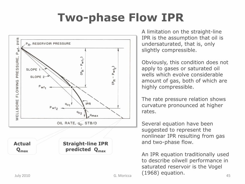
Two-phase Flow IPR
July 2010 G. Moricca 45
Actual Qmax
Straight-line IPRpredicted Qmax
A limitation on the straight-line IPR is the assumption that oil is undersaturated, that is, only slightly compressible.
Obviously, this condition does not apply to gases or saturated oil wells which evolve considerable amount of gas, both of which are highly compressible.
The rate pressure relation shows curvature pronounced at higher rates.
Several equation have been suggested to represent the nonlinear IPR resulting from gas and two-phase flow.
An IPR equation traditionally used to describe oilwell performance in saturated reservoir is the Vogel (1968) equation.
Vogel’s equation
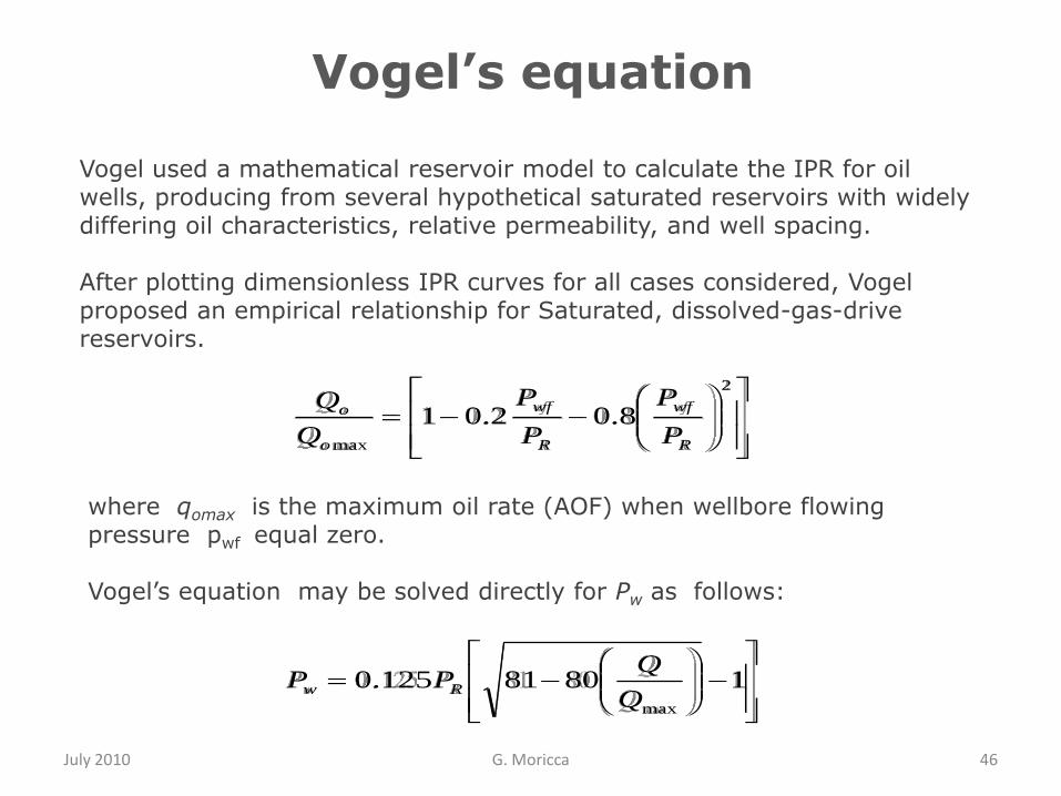
July 2010 G. Moricca 46
Vogel used a mathematical reservoir model to calculate the IPR for oil wells, producing from several hypothetical saturated reservoirs with widely differing oil characteristics, relative permeability, and well spacing.
After plotting dimensionless IPR curves for all cases considered, Vogel proposed an empirical relationship for Saturated, dissolved-gas-drive reservoirs.
2
max
8.02.01R
wf
R
wf
o
o
P
P
P
P
Q
Q
where qomax is the maximum oil rate (AOF) when wellbore flowing pressure pwf equal zero.
Vogel‟s equation may be solved directly for Pw as follows:
18081125.0
maxQ
QPP Rw
Use of Vogel’s IPR equation
July 2010 G. Moricca 47
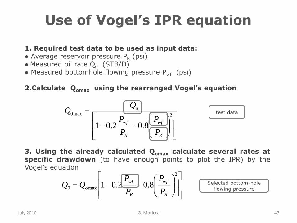
1. Required test data to be used as input data:● Average reservoir pressure PR (psi)● Measured oil rate Qo (STB/D)● Measured bottomhole flowing pressure Pwf (psi)
2.Calculate Qomax using the rearranged Vogel’s equation
3. Using the already calculated Qomax calculate several rates atspecific drawdown (to have enough points to plot the IPR) by theVogel‟s equation
2max0
8.02.01R
wf
R
wf
o
P
P
P
P
QQ test data
2
max0 8.02.01R
wf
R
wf
oP
P
P
PQQ Selected bottom-hole
flowing pressure

July 2010 G. Moricca 48
WorkshopSession
-Vogel’s IPR

Workshop: Vogel’s IPR
July 2010 G. Moricca 49
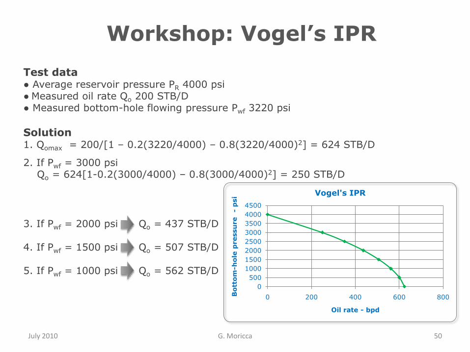
Problem
A discovery well was tested at a rate of 200 STB/D with a bottom-hole
flowing pressure of 3220 psia. Bubble-point pressure was calculated with a
correlation using surface data measured when the well was producing at a low
rate. The estimated bubble point of 3980 psia indicates that the well is
draining saturated oil, since initial reservoir pressure was measured at
4000 psia.
Plot the IPR using Vogel equation.
2max0
8.02.01R
wf
R
wf
o
P
P
P
P
2
max0 8.02.01R
wf
R
wf
oP
P
P
PQQ
July 2010 G. Moricca 50
Test data● Average reservoir pressure PR 4000 psi● Measured oil rate Qo 200 STB/D● Measured bottom-hole flowing pressure Pwf 3220 psi
Solution1. Qomax = 200/[1 – 0.2(3220/4000) – 0.8(3220/4000)2] = 624 STB/D
2. If Pwf = 3000 psiQo = 624[1-0.2(3000/4000) – 0.8(3000/4000)2] = 250 STB/D
3. If Pwf = 2000 psi Qo = 437 STB/D
4. If Pwf = 1500 psi Qo = 507 STB/D
5. If Pwf = 1000 psi Qo = 562 STB/D
Workshop: Vogel’s IPR
0
500
1000
1500
2000
2500
3000
3500
4000
4500
0 200 400 600 800Bott
om
-ho
le p
ressu
re
-p
si
Oil rate - bpd
Vogel's IPR

Reservoir Inflow Performance: Summary
July 2010 G. Moricca 51
Inflow Performance Relationship (IPR ) is routinely measured using bottom hole pressure gauges at regular intervals as part of the field monitoring programme.
● Well Producing undersaturatedoil (no gas at the wellbore) or water have a straight line IPR
● PI is a useful tool for comparing wells since it combines all the relevant rock, fluid and geometry properties into a single value to describe (relative) inflow performance.
● AOF : Absolute Open hole Factor is the flow rate at zero (bottom hole) wellbore flowing pressure.
● AOF is useful parameter when comparing wells within a field since it combines PI and reservoir pressure in one number representative of well inflow potential.
cont/...
Reservoir Inflow Performance: Summary
July 2010 G. Moricca 52
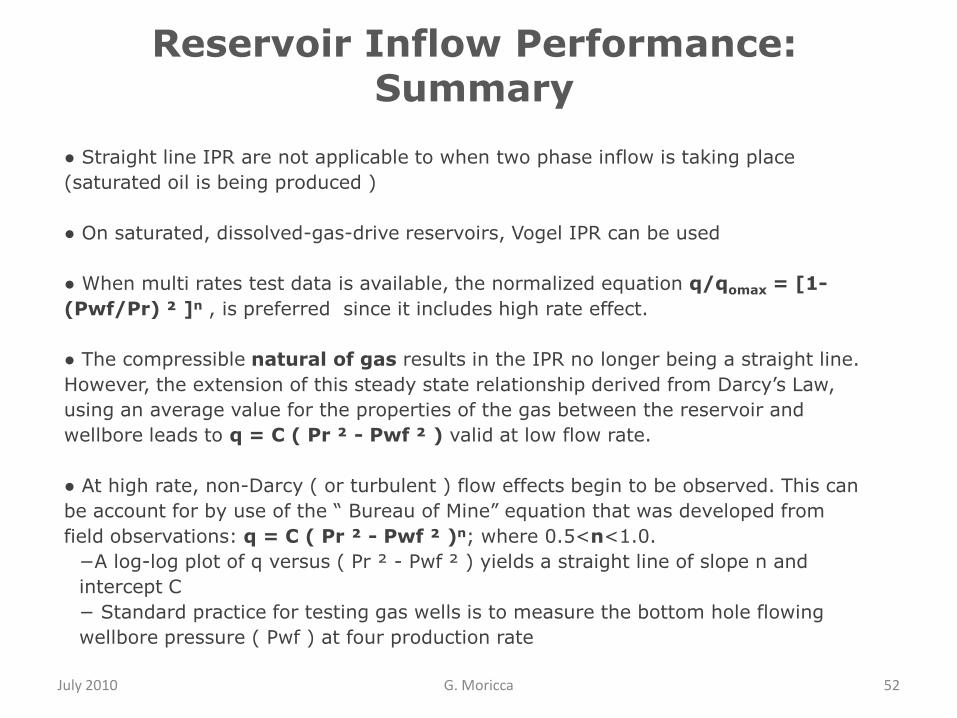
● Straight line IPR are not applicable to when two phase inflow is taking place
(saturated oil is being produced )
● On saturated, dissolved-gas-drive reservoirs, Vogel IPR can be used
● When multi rates test data is available, the normalized equation q/qomax = [1-
(Pwf/Pr) ² ]n , is preferred since it includes high rate effect.
● The compressible natural of gas results in the IPR no longer being a straight line.
However, the extension of this steady state relationship derived from Darcy‟s Law,
using an average value for the properties of the gas between the reservoir and
wellbore leads to q = C ( Pr ² - Pwf ² ) valid at low flow rate.
● At high rate, non-Darcy ( or turbulent ) flow effects begin to be observed. This can
be account for by use of the “ Bureau of Mine” equation that was developed from
field observations: q = C ( Pr ² - Pwf ² )n; where 0.5<n<1.0.
−A log-log plot of q versus ( Pr ² - Pwf ² ) yields a straight line of slope n and
intercept C
− Standard practice for testing gas wells is to measure the bottom hole flowing
wellbore pressure ( Pwf ) at four production rate

July 2010 G. Moricca 53
Well
Deliverability-
Outflowor
Tubing Performance
July 2010 G. Moricca 54
At the end of this section, you will be able to…
● Calculate Friction Pressure losses assuming NO gas.
● Calculate the Outflow Pressure for a given set of conditions.
● Calculate the Outflow pressure against variable flow rates: Tubing
intake Curve.
● Plot the Outflow Curve or Tubing Performance Relationship (TPR).
● Use of the Kermit E. Brown‟s Vertical Flowing Pressure Gradient
working graphs to estimate the tubing intake pressure .
● Understand the effect on the TPR and the Pressure Traverse of the
pressure-loss components: Well-head Back Pressure (THP);
Hydrostatic, and Friction.
● Understand the different behavior of single-phase fluid, dry gas and
multiphase mixture, in terms of TPR and Pressure Traverse.
Well DeliverabilityOutflow or Tubing Performance
July 2010 G. Moricca 55
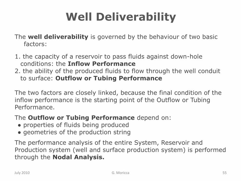
The well deliverability is governed by the behaviour of two basic factors:
1. the capacity of a reservoir to pass fluids against down-hole conditions: the Inflow Performance
2. the ability of the produced fluids to flow through the well conduit to surface: Outflow or Tubing Performance
The two factors are closely linked, because the final condition of the inflow performance is the starting point of the Outflow or Tubing Performance.
The Outflow or Tubing Performance depend on:● properties of fluids being produced● geometries of the production string
The performance analysis of the entire System, Reservoir and Production system (well and surface production system) is performed through the Nodal Analysis.
Well Deliverability

July 2010 G. Moricca 56
Well Deliverability
OPERATINGPOINT
QACTUALP
AC
TU
AL
NATURAL FLOWING WELLDEAD WELL
Flow rate Q
Pressu
re P
Outflow(TPR)
Inflow(IPR)

July 2010 G. Moricca 57
Well Deliverability
TPR
PI1 < PI2 < PI3

July 2010 G. Moricca 58
Well Deliverability
TPR
Well DeliverabilityOutflow or Tubing Performance
July 2010 G. Moricca 59
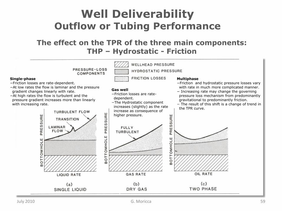
The effect on the TPR of the three main components:
THP – Hydrostatic - Friction
Single-phase−Friction losses are rate-dependent.−At low rates the flow is laminar and the pressure gradient changes linearly with rate.
−At high rates the flow is turbulent and the pressure gradient increases more than linearly with increasing rate.
Multiphase−Friction and hydrostatic pressure losses vary with rate in much more complicated manner.
− Increasing rate may change the governing pressure loss mechanism from predominantly gravitational to predominantly friction.
− The result of this shift is a change of trend in the TPR curve.
Gas well−Friction losses are rate-dependent.
−The Hydrostatic component increases (slightly) as the rate increase as consequence of higher pressure.

July 2010 G. Moricca 60
Tubing (Outflow) Performance
In terms the number of factors that determine the outflow
behaviour, outflow is more complicated than inflow.
The factors that affect outflow are:
● Tubing Wellhead Pressure
● Vertical Depth
● Flowing Fluid Properties (WC, GOR, oil density, fluid viscosity)
● Geometry (well deviation)
● Flow regime:
− single phase (laminar or turbulent),
− multiphase, (slug flow, annular flow, etc.)
● Tubing size, weight, and surface roughness
● Flow Rate
Well DeliverabilityOutflow or Tubing Performance
July 2010 G. Moricca 61
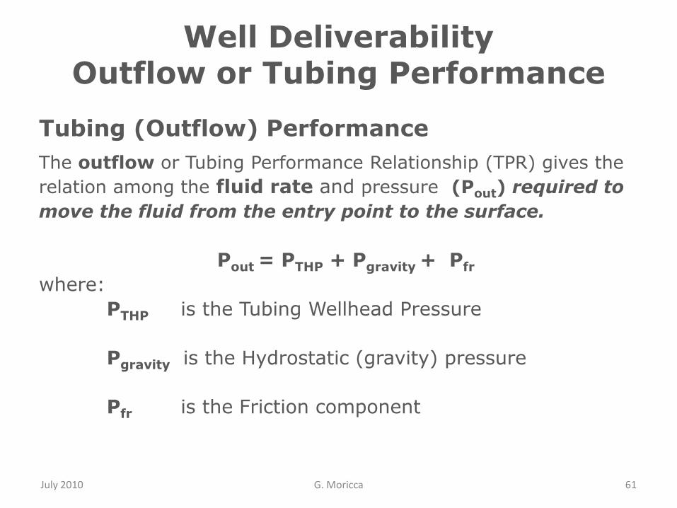
Tubing (Outflow) Performance
The outflow or Tubing Performance Relationship (TPR) gives the
relation among the fluid rate and pressure (Pout) required to
move the fluid from the entry point to the surface.
Pout = PTHP + Pgravity + Pfr
where:
PTHP is the Tubing Wellhead Pressure
Pgravity is the Hydrostatic (gravity) pressure
Pfr is the Friction component
Well DeliverabilityOutflow or Tubing Performance
July 2010 G. Moricca 62
Pressure losses in the tubing:Hydrostatic (gravity) pressure component
● Pgravity is simply determined by the vertical depth (elevation)
and the average fluid gradient (Fluid gradient = Fluid
density /144, in field units) of the fluid in the tubing.
● To find a pressure (Pgravity) at a given depth (D), simplymultiply the VERTICAL depth (elevation) by the given fluidaverage gradient (Gavg).
Pgravity = D x Gavg
Well DeliverabilityOutflow or Tubing Performance

July 2010 G. Moricca 63
Pressure losses in the tubing:Frictional pressure losses component
● Friction is quite more complicated than the other two Pressure losses
components.
● As noted above, friction depends on „everything else‟. This means that the
fluid phases, flow regime, well deviation and profile, fluid viscosity,
and tubing size all determine friction.
● Even without gas, there are several possible ways to estimate the friction in
a pipe due to flow. Examples are the Darcy-Weisbach equation and the
Moody diagram.
● One of the most used is the Hazen-Williams formula for friction losses in
water pipes.
● The Hazen–Williams equation is an empirical formula which relates the flow
of water in a pipe with the physical properties of the pipe and the pressure
drop caused by friction.
● The Hazen–Williams equation has the advantage that is not a function of the
Reynolds number, but it has the disadvantage that it is only valid for water,
NO gas.
Well DeliverabilityOutflow or Tubing Performance
Well DeliverabilityOutflow or Tubing Performance
July 2010 G. Moricca 64
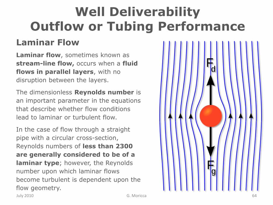
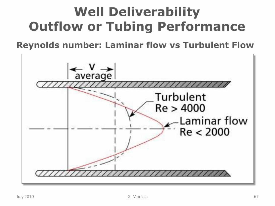
Laminar Flow
Laminar flow, sometimes known as
stream-line flow, occurs when a fluid
flows in parallel layers, with no
disruption between the layers.
The dimensionless Reynolds number is
an important parameter in the equations
that describe whether flow conditions
lead to laminar or turbulent flow.
In the case of flow through a straight
pipe with a circular cross-section,
Reynolds numbers of less than 2300
are generally considered to be of a
laminar type; however, the Reynolds
number upon which laminar flows
become turbulent is dependent upon the
flow geometry.
Well DeliverabilityOutflow or Tubing Performance
July 2010 G. Moricca 65
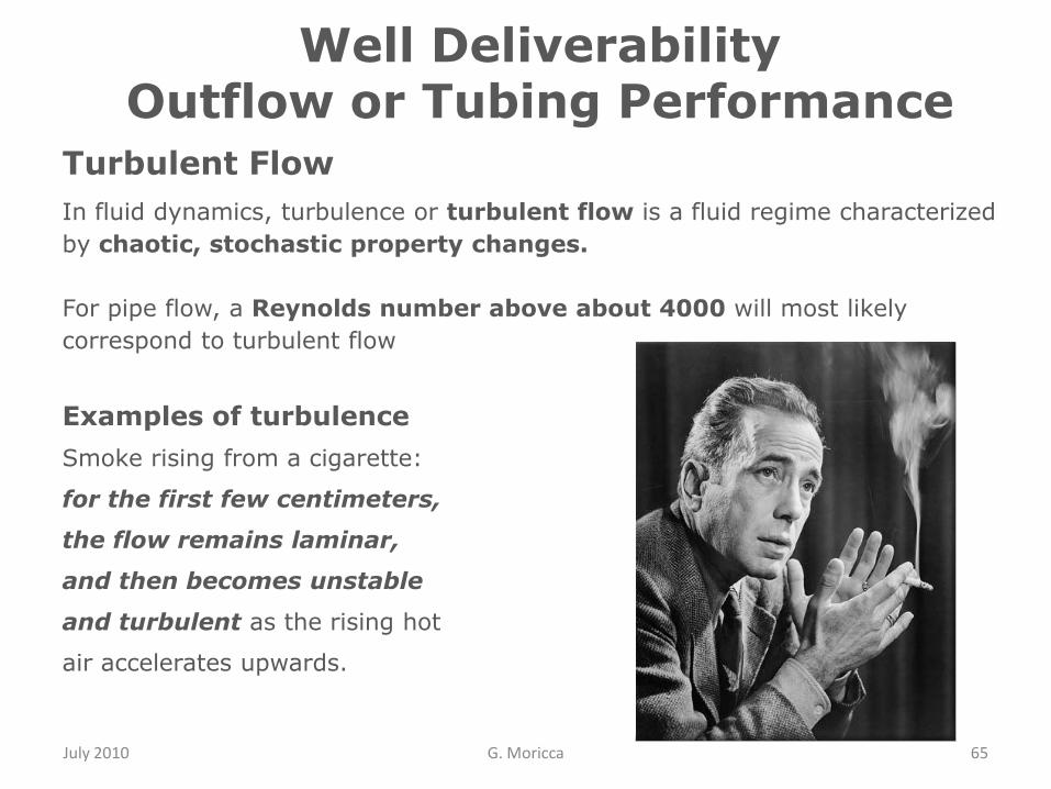
Turbulent Flow
In fluid dynamics, turbulence or turbulent flow is a fluid regime characterized
by chaotic, stochastic property changes.
For pipe flow, a Reynolds number above about 4000 will most likely
correspond to turbulent flow
Examples of turbulence
Smoke rising from a cigarette:
for the first few centimeters,
the flow remains laminar,
and then becomes unstable
and turbulent as the rising hot
air accelerates upwards.
Well DeliverabilityOutflow or Tubing Performance
July 2010 G. Moricca 66
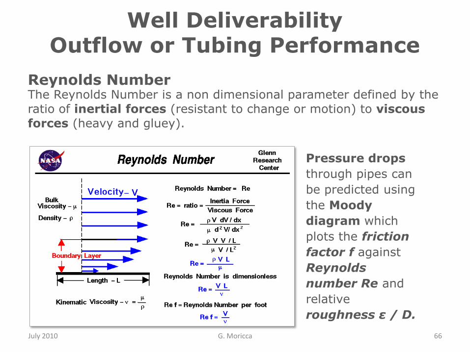
Reynolds NumberThe Reynolds Number is a non dimensional parameter defined by the
ratio of inertial forces (resistant to change or motion) to viscous
forces (heavy and gluey).
Pressure drops
through pipes can
be predicted using
the Moody
diagram which
plots the friction
factor f against
Reynolds
number Re and
relative
roughness ε / D.
Well DeliverabilityOutflow or Tubing Performance
July 2010 G. Moricca 67
Reynolds number: Laminar flow vs Turbulent Flow

Well DeliverabilityOutflow or Tubing Performance
July 2010 G. Moricca 68
Moody Diagram: Friction Factor vs Reynolds Number
Please note that
being Reynolds
Number
proportional to the
velocity (fluid rate)
and, in turn, the
fluid rate is
proportional to the
Friction factor, a
trial an error
calculation process
is required to
identify the friction
factor f.

Well DeliverabilityMultiphase Flow in Vertical Tubing
July 2010 G. Moricca 69
Flow pattern of Multiphase Flow
When the wellbore flowing pressure is greater than the bubble point
pressure, single phase oil is entering the well. Single phase flow
will continue until the pressure reduce sufficiently that the
bubble point is reached.
The flow patterns in the tubing that will result from this gas bubble
formation is a function of:
● Gas and Liquid flow rate
● Pipe angle of inclination
● Pipe diameter
● Phase density
Well DeliverabilityMultiphase Flow in Vertical Tubing
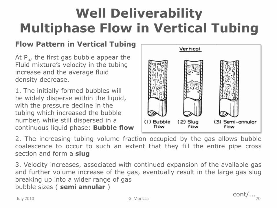
July 2010 G. Moricca 70
Flow Pattern in Vertical Tubing
At Pb, the first gas bubble appear theFluid mixture‟s velocity in the tubingincrease and the average fluiddensity decrease.
1. The initially formed bubbles willbe widely disperse within the liquid,with the pressure decline in thetubing which increased the bubblenumber, while still dispersed in acontinuous liquid phase: Bubble flow
2. The increasing tubing volume fraction occupied by the gas allows bubblecoalescence to occur to such an extent that they fill the entire pipe crosssection and form a slug
3. Velocity increases, associated with continued expansion of the available gasand further volume increase of the gas, eventually result in the large gas slugbreaking up into a wider range of gasbubble sizes ( semi annular )
cont/...

July 2010 G. Moricca 71
4. Further upward fluid flow continues the gasliberation and expansion processes so thatthe phases separate into a central, highvelocity core of gas with a continuous filmof liquid on the tubing wall – The annularflow regime.
5. Shear at the gas/liquid interface resultingfrom continually increasing gas velocitieswill eventually destroy the annular ring ofliquid on the tubing wall and disperse it asa mist of small droplet – the Mist flowregime.
Well DeliverabilityMultiphase Flow in Vertical Tubing
July 2010 G. Moricca 72
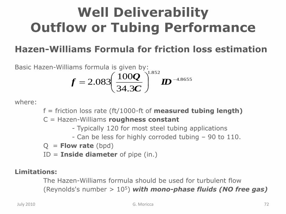
Hazen-Williams Formula for friction loss estimation
Basic Hazen-Williams formula is given by:
where:
f = friction loss rate (ft/1000-ft of measured tubing length)
C = Hazen-Williams roughness constant
- Typically 120 for most steel tubing applications
- Can be less for highly corroded tubing – 90 to 110.
Q = Flow rate (bpd)
ID = Inside diameter of pipe (in.)
Limitations:
The Hazen-Williams formula should be used for turbulent flow
(Reynolds's number > 105) with mono-phase fluids (NO free gas)
Well DeliverabilityOutflow or Tubing Performance
8655.4
852.1
3.34
100083.2
ID
C
Qf
July 2010 G. Moricca 73
Hazen-Williams Formula for friction loss estimation
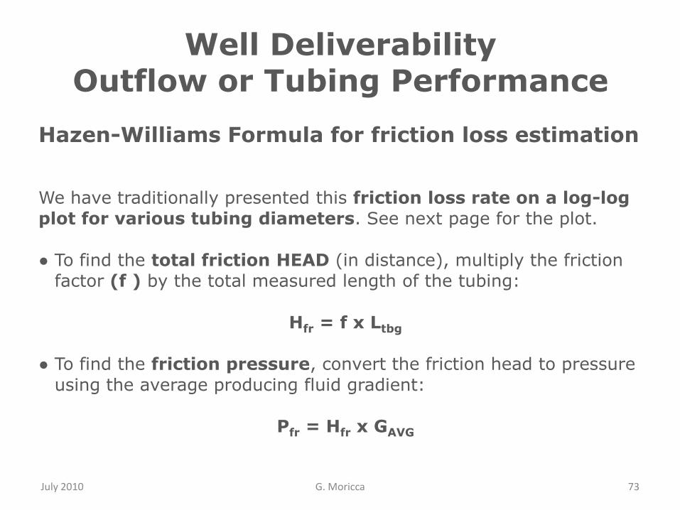
We have traditionally presented this friction loss rate on a log-log
plot for various tubing diameters. See next page for the plot.
● To find the total friction HEAD (in distance), multiply the friction
factor (f ) by the total measured length of the tubing:
Hfr = f x Ltbg
● To find the friction pressure, convert the friction head to pressure
using the average producing fluid gradient:
Pfr = Hfr x GAVG
Well DeliverabilityOutflow or Tubing Performance
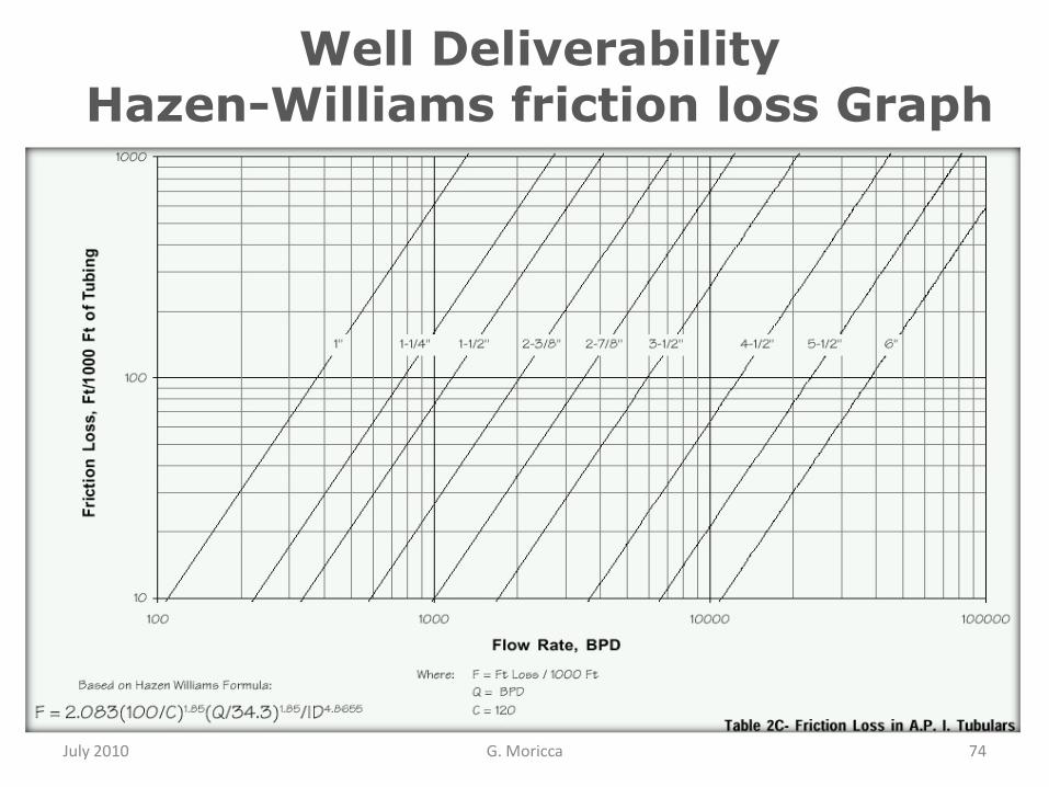
Well DeliverabilityHazen-Williams friction loss Graph
July 2010 G. Moricca 74
July 2010 G. Moricca 75
WorkshopSession
-Outflow or Tubing
Performance
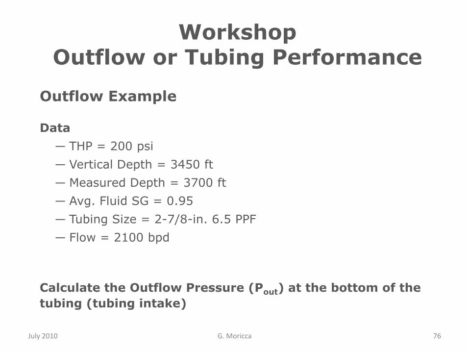
WorkshopOutflow or Tubing Performance
July 2010 G. Moricca 76
Outflow Example
Data
― THP = 200 psi
― Vertical Depth = 3450 ft
― Measured Depth = 3700 ft
― Avg. Fluid SG = 0.95
― Tubing Size = 2-7/8-in. 6.5 PPF
― Flow = 2100 bpd
Calculate the Outflow Pressure (Pout) at the bottom of the
tubing (tubing intake)

July 2010 G. Moricca 77
Outflow Example - Solution
Pout = PTHP + Pgravity + Pfr
1. PTHP = 200 psi
2. Pgravity = Fluid Gradient x Elevation
Fluid Gradient = Fluid density / 144
Fluid density = Fluid Specific Gravity (water =1) x 62.3
Fluid Gradient = (Fluid SG x 62.3)/144 =
= (0.95 x 62.3)/144 = 0.411 psi/ft
Pgravity = 0.411 x 3450 = 1418 psi
Remember that 62.3 is the water density in lb/cu ft; 1 in2 = 144 ft2 and
therefore:
cont/....
ft
psi
inft
lb
in
ft
ft
lb433.0433.0
144
13.62
222
2
3
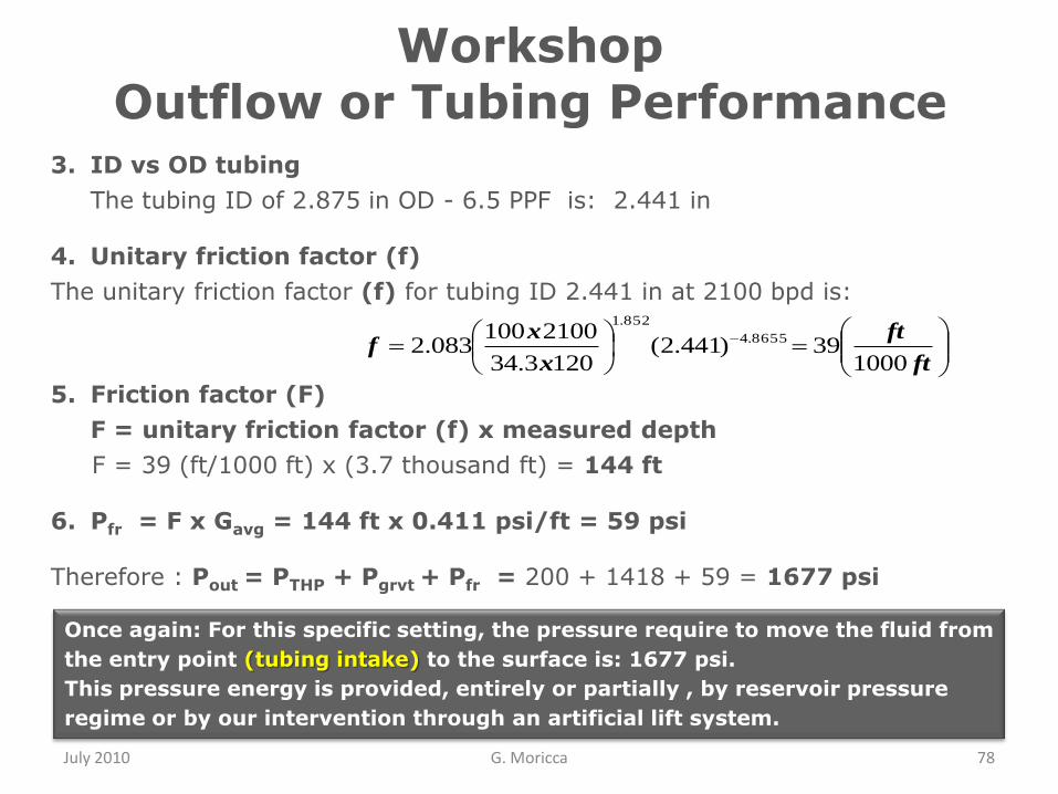
WorkshopOutflow or Tubing Performance
July 2010 G. Moricca 78
3. ID vs OD tubing
The tubing ID of 2.875 in OD - 6.5 PPF is: 2.441 in
4. Unitary friction factor (f)
The unitary friction factor (f) for tubing ID 2.441 in at 2100 bpd is:
5. Friction factor (F)
F = unitary friction factor (f) x measured depth
F = 39 (ft/1000 ft) x (3.7 thousand ft) = 144 ft
6. Pfr = F x Gavg = 144 ft x 0.411 psi/ft = 59 psi
Therefore : Pout = PTHP + Pgrvt + Pfr = 200 + 1418 + 59 = 1677 psi
ft
ft
x
xf
100039)441.2(
1203.34
2100100083.2 8655.4
852.1
Once again: For this specific setting, the pressure require to move the fluid from
the entry point (tubing intake) to the surface is: 1677 psi.
This pressure energy is provided, entirely or partially , by reservoir pressure
regime or by our intervention through an artificial lift system.
WorkshopOutflow or Tubing Performance
July 2010 G. Moricca 79
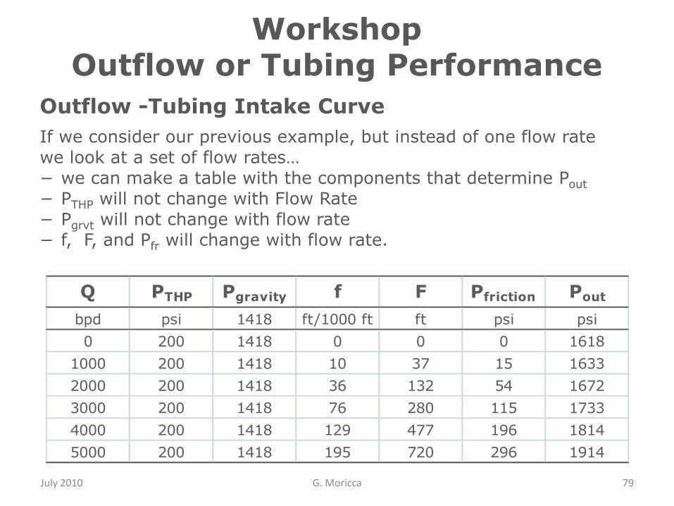
Outflow -Tubing Intake Curve
If we consider our previous example, but instead of one flow rate
we look at a set of flow rates…
− we can make a table with the components that determine Pout
− PTHP will not change with Flow Rate
− Pgrvt will not change with flow rate
− f, F, and Pfr will change with flow rate.
Q PTHP Pgravity f F Pfriction Pout
bpd psi 1418 ft/1000 ft ft psi psi
0 200 1418 0 0 0 1618
1000 200 1418 10 37 15 1633
2000 200 1418 36 132 54 1672
3000 200 1418 76 280 115 1733
4000 200 1418 129 477 196 1814
5000 200 1418 195 720 296 1914
WorkshopOutflow or Tubing Performance
July 2010 G. Moricca 80
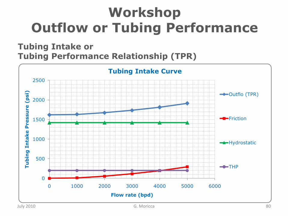
Tubing Intake orTubing Performance Relationship (TPR)
0
500
1000
1500
2000
2500
0 1000 2000 3000 4000 5000 6000
Tu
bin
g I
nta
ke P
ressu
re (
psi)
Flow rate (bpd)
Tubing Intake Curve
Outflo (TPR)
Friction
Hydrostatic
THP
WorkshopOutflow or Tubing Performance
Well DeliverabilityOutflow or Tubing Performance
July 2010 G. Moricca 81
Vertical Flowing Pressure Gradient orPressure Traverse
For a given flow rate, well-head pressure and tubing size, there is
a particular pressure distribution along the tubing, starting its
traverse at the well-head pressure and increasing downward
toward the intake to the tubing.
The pressure-depth profile is called a Vertical Flowing Pressure
Gradient or Pressure Traverse.
The tubing intake pressure can be also estimated by use of the
Vertical Flowing Pressure Gradient working graphs.
In the next pages the step-by-step procedure to obtain the
bottom-hole flowing pressure (intake pressure) from the well-
head flowing pressure (and vice versa), by use of Kermit E.
Brown‟s working graphs will be illustrated.
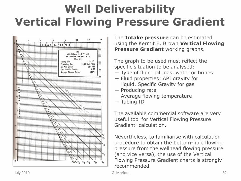
Well DeliverabilityVertical Flowing Pressure Gradient
July 2010 G. Moricca 82
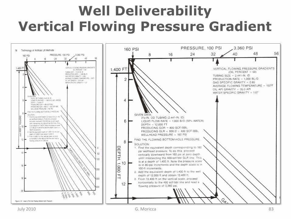
The Intake pressure can be estimated using the Kermit E. Brown Vertical Flowing Pressure Gradient working graphs.
The graph to be used must reflect the specific situation to be analysed:― Type of fluid: oil, gas, water or brines― Fluid properties: API gravity for
liquid, Specific Gravity for gas― Producing rate― Average flowing temperature― Tubing ID
The available commercial software are very useful tool for Vertical Flowing Pressure Gradient calculation.
Nevertheless, to familiarise with calculation procedure to obtain the bottom-hole flowing pressure from the wellhead flowing pressure (and vice versa), the use of the Vertical Flowing Pressure Gradient charts is strongly recommended.
July 2010 G. Moricca 83
Well DeliverabilityVertical Flowing Pressure Gradient

July 2010 G. Moricca 84
Well DeliverabilityVertical Flowing Pressure Gradient
July 2010 G. Moricca 85
Well DeliverabilityVertical Flowing Pressure Gradient
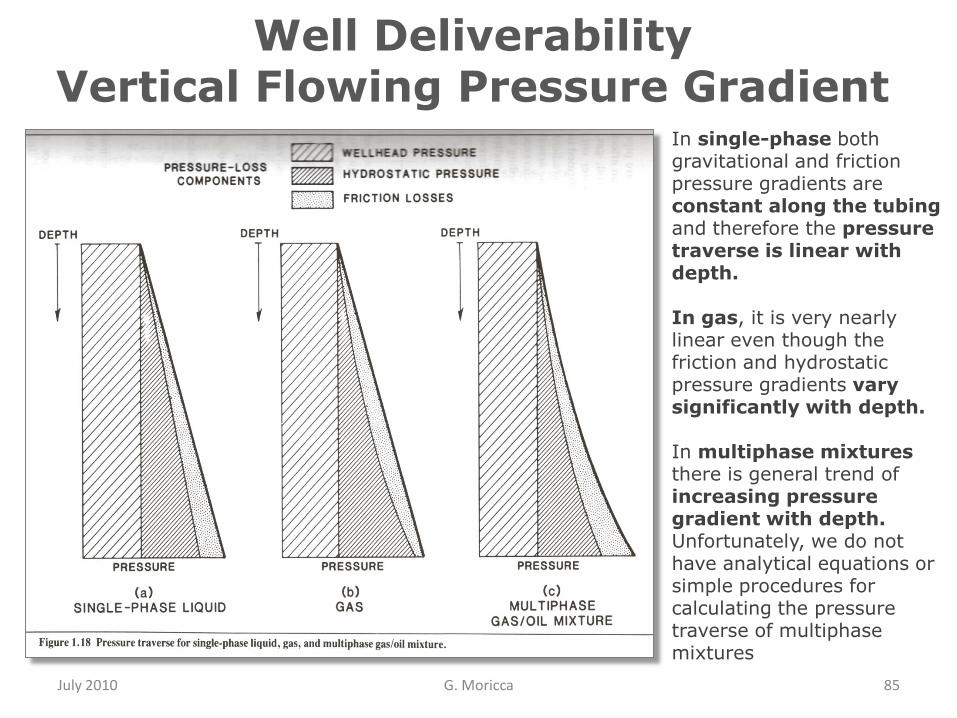
In single-phase both gravitational and friction pressure gradients are constant along the tubing and therefore the pressure traverse is linear with depth.
In gas, it is very nearly linear even though the friction and hydrostatic pressure gradients vary significantly with depth.
In multiphase mixtures there is general trend of increasing pressure gradient with depth.Unfortunately, we do not have analytical equations or simple procedures for calculating the pressure traverse of multiphase mixtures
Well Deliverability
July 2010 G. Moricca 86
Summary
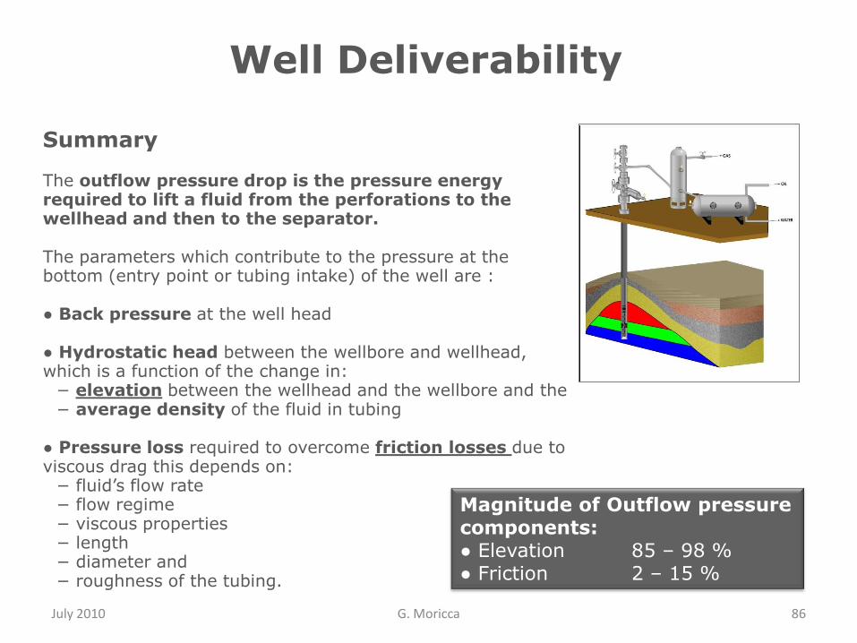
The outflow pressure drop is the pressure energy required to lift a fluid from the perforations to the wellhead and then to the separator.
The parameters which contribute to the pressure at the bottom (entry point or tubing intake) of the well are :
● Back pressure at the well head
● Hydrostatic head between the wellbore and wellhead, which is a function of the change in:
− elevation between the wellhead and the wellbore and the− average density of the fluid in tubing
● Pressure loss required to overcome friction losses due to viscous drag this depends on:
− fluid‟s flow rate− flow regime − viscous properties− length− diameter and− roughness of the tubing.
Magnitude of Outflow pressurecomponents:● Elevation 85 – 98 %● Friction 2 – 15 %

July 2010 G. Moricca 87
SystemPerformance
Analysis-
Nodal Analysis
July 2010 G. Moricca 88
System deliverability
At the end of this section, you will be able to…
● Understand the effect on the overall System deliverability
of the following parameters:
― Productivity Index
― Reservoir Pressure
― Skin effect
― Water cut
― Tubing ID
― Well-head flowing pressure

Nodal Analysis
July 2010 G. Moricca 89
To simulate the fluid flow in the system, it is necessary to “break” the system into discrete nodes that separate system elements.
Nodal analysis is performed on the principle of pressure continuity, that is, there is only one unique pressure value at a given node regardless of whether the pressure is evaluated from the performance of upstream equipment or downstream equipment.
The performance curve (pressure-rate relation) of upstream equipment is called inflow performance curve; the performance curve of downstream equipment is called out flow performance curve.
The intersection of the two performance curves define the operating point, that is, operating flow rate and pressure, at the specified node.
For the convenience of using pressure data measured normally at either the bottom-hole or the wellhead, Nodal analysis is usually conducted using the bottom-hole or the wellhead as the solution node.
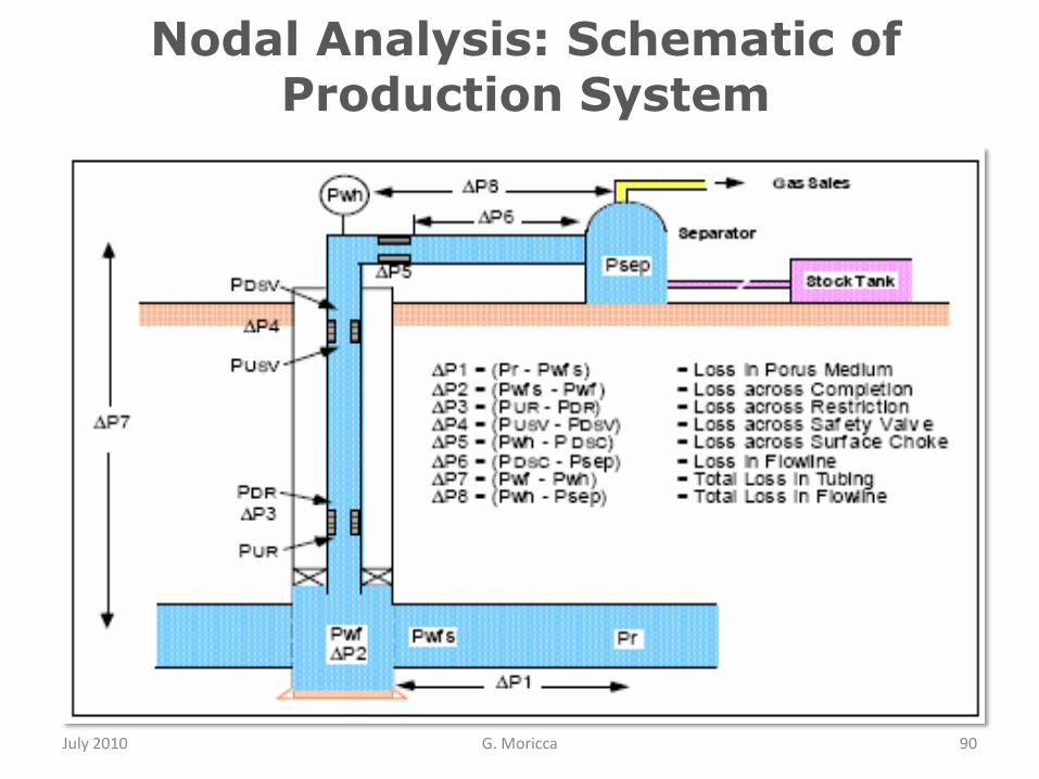
Nodal Analysis: Schematic of Production System
July 2010 G. Moricca 90

Nodal Analysis: Locations of nodes
July 2010 G. Moricca 91
System Analysis consists of:
Selecting a point or node within the production system (well and surface facilities)
Equations for the relationship between flow rate and pressure drop are then developed for the well components both upstream of the node (inflow) and downstream (outflow)
The flow rate and pressure at the node can be calculated since: –Flow into the node equals flow out of the node.–Only one pressure can exist at the node

System Deliverability vs Productivity Index
July 2010 G. Moricca 92

System Deliverability vs Reservoir Pressure
July 2010 G. Moricca 93
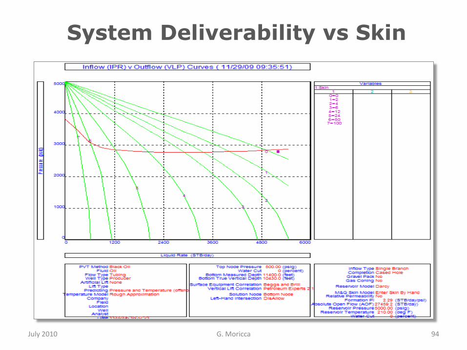
System Deliverability vs Skin
July 2010 G. Moricca 94
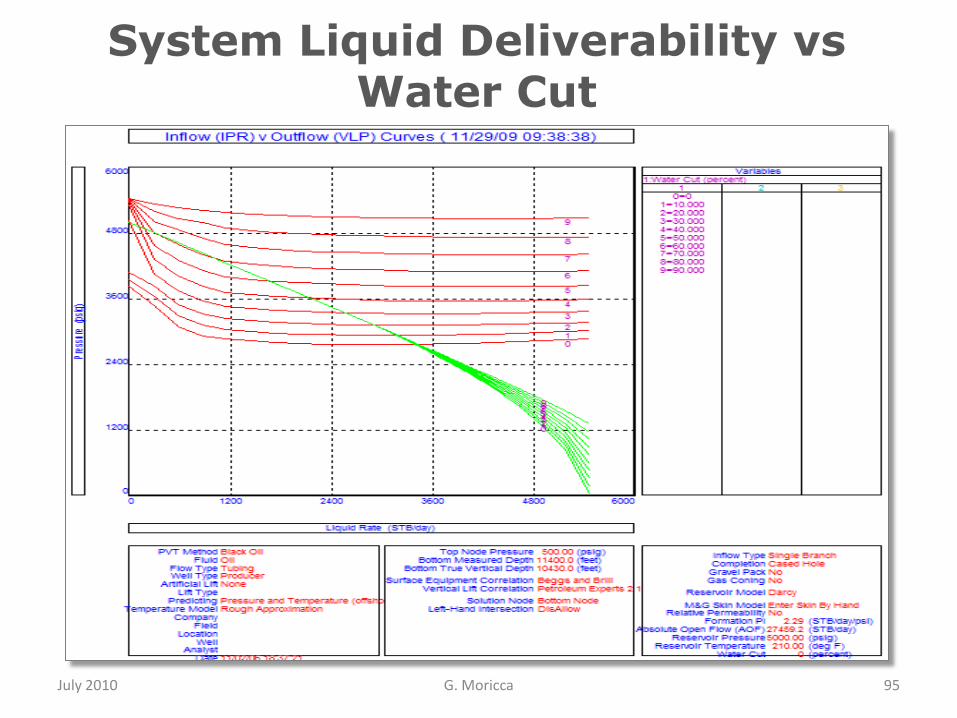
System Liquid Deliverability vsWater Cut
July 2010 G. Moricca 95

System Oil Deliverability vs Water Cut
July 2010 G. Moricca 96

System Deliverability vs TGB ID
July 2010 G. Moricca 97

July 2010 G. Moricca 98
Fundamental
of
Artificial Lift
Main source: Well Performance. M. Golan /C. H. Whitson. Prentice Hall Inc

July 2010 G. Moricca 99
Fundamental of Artificial Lift
At the end of this section, you will be able to
understand the basic of:
― Gas Lift
― Electrical Submersible Pump (ESP)
― Hydraulic Submersible Pump (HSP)
― Jet Pump
― Progressive Cavity Pump (PCP)
― Beam or Sucker Rod Pump
Fundamental of Artificial Lift
July 2010 G. Moricca 100
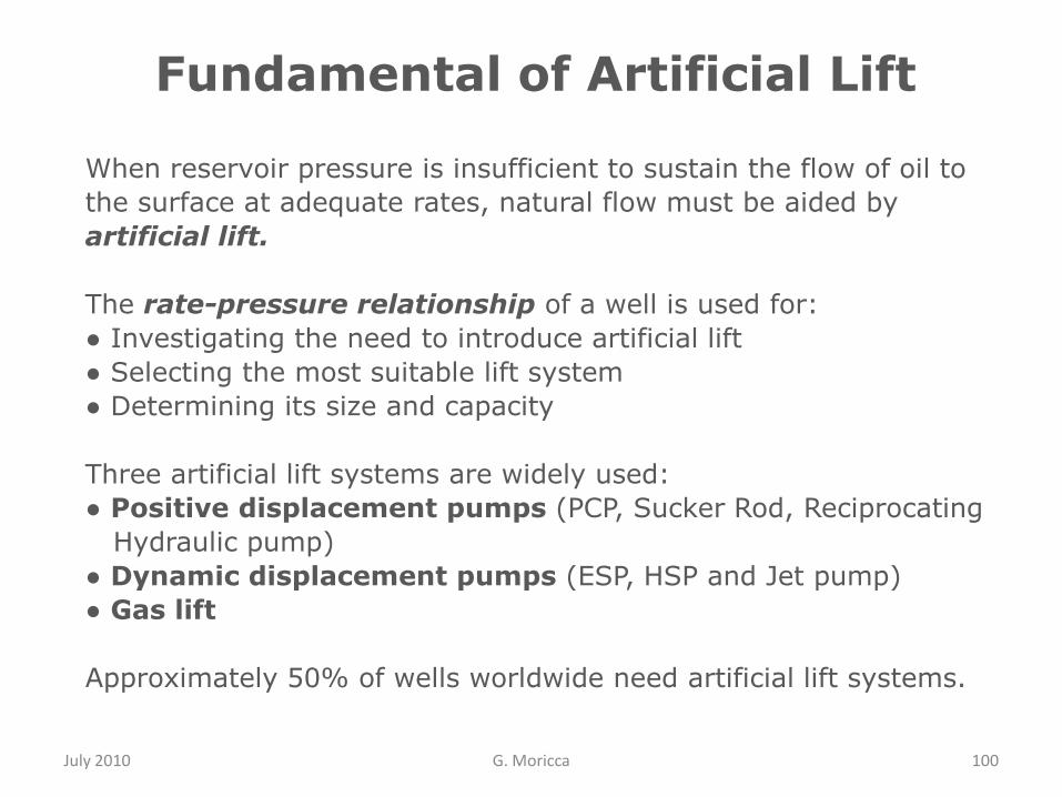
When reservoir pressure is insufficient to sustain the flow of oil to
the surface at adequate rates, natural flow must be aided by
artificial lift.
The rate-pressure relationship of a well is used for:
● Investigating the need to introduce artificial lift
● Selecting the most suitable lift system
● Determining its size and capacity
Three artificial lift systems are widely used:
● Positive displacement pumps (PCP, Sucker Rod, Reciprocating
Hydraulic pump)
● Dynamic displacement pumps (ESP, HSP and Jet pump)
● Gas lift
Approximately 50% of wells worldwide need artificial lift systems.

Methods of Artificial Lift
July 2010 G. Moricca 101
There are two basic forms of continuous artificial lift:● Downhole pump● Gas lift
Downhole pumps boost the transfer of liquid from the bottom-hole to the wellhead eliminating backpressure caused by the fluid flowing in the tubing.
Injection of gas into the production string aerates the flowing fluid reducing the pressure gradient and lowering backpressure at the formation.
For both lift methods, the production rate is increased by reducing wellbore flowing pressure.
The understanding of relationships among the pressure gradient
(backpressure) and bottom-hole flow condition to make possible the
flow is a fundamental step to design the Artificial Lift System and
select the proper action for its optimization.
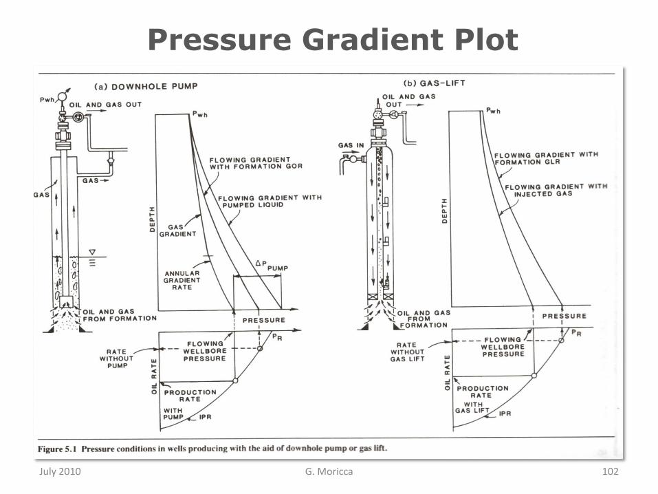
Pressure Gradient Plot
July 2010 G. Moricca 102

Pressure Gradient Plot Analysis
July 2010 G. Moricca 103
● The IPR curve relates the wellbore flowing pressure Pwf to flow rate at the surface.
● The pressure traverse curve, at given wellhead pressure, determines the tubing intake backpressure Pin at a particular flow rate.
● Stable production can only exist if these two pressure Pwf
and Pin are equal.
In the pumping well, the pump provides the pressure
difference (Pin ― Pwf ) needed to overcome tubing
backpressure and sustain stable flow

Pressure Gradient Plot Analysis
July 2010 G. Moricca 104
The Pressure Gradient Plot indicates the limit on production rate achievable by each lifting method:
● Down-hole pumps may withdraw reservoir fluid at rate approaching the absolute open flow (AOF).
● In gas lift backpressure exerted by the flowing fluid column limits the reduction of wellbore flowing pressure and thus limits production to a rate significantly less than the AOF.
An important observation in the pressure diagram is that there exists a relationship between the:
― wellbore flowing pressure― liquid level in the annulus― casing backpressure
This relationship plays a significant role in determining the pump setting depth and its allowable pumping rate.
In pumping well, it is mandatory to settle the pump below the free gas-liquid contact. The free gas is intentionally segregated from the liquid before fluid enters the pump, being vented to the surface through the tubing/casing annulus. Eliminating free gas in pumps is a fundamental requirement for efficient pumping.
Quick-look of Artificial Lift
Systems
July 2010 G. Moricca 105
Main sources:
‒ Well Completion Design. Jonathan Bellarby. Elsevier Inc
‒ Schlumberger Oilfield Review
‒ Electrical Submersible Pumps Manual. Gabor Takacs. Elsevier Inc

Quick-look of Artificial Lift Systems
July 2010 G. Moricca 106
The basic information (concept, application, positive and negative
features) concerning the following Artificial Systems will be
provided:
Gas Lift
Electrical Submersible Pump (ESP)
Hydraulic Submersible Pump (HSP)
Jet Pump
Progressive Cavity Pump (PCP)
Beam or Sucker Rod Pump

Gas Lift
July 2010 G. Moricca 107
Gas lift consist of injecting high pressure gas from the surface to apredetermined tubing string depth to decrease fluid density in wellboretherefore reducing the hydrostatic load on formations which will allowreservoir energy to cause inflow and commercial hydrocarbon volumes canbe boosted or displaced to the Surface.
The gas injected through the operating valve in the tubing string enables the well to resume or increase production by:
● reducing the average fluid density above the injection point
● some of the injected gas dissolvinginto the produced fluids(undersaturated ) and the remainingin form of bubbles will expand as thefluid rise up the tubing string
July 2010 G. Moricca 108
Advantages
● Preferred method for wells with:– High gas oil ratio– High productivity index– Relatively high bottom hole pressure
● Suitable for medium rate
● Suitable for water drive reservoirs withhigh bottom-hole pressure
● Provides full bore tubing string access
● Low operational and maintenance cost
● Flexibility: can handle rates from 10 to 20.000 bpd
● Can handle (tolerate) produced solids
● Low surface profile, importantfor offshore / Urban locations
Disadvantages
● Gas has to be available
● Possible high installation cost– Compressor installation– Modifications to existing platforms
● Gas lifting of viscous crude (<15 API )is difficult and less efficient
● Difficult restart after shut down
● Wax precipitation problem may increase due to cooling effect from gas injection & subsequent expansion
● Hydrate blocking surface gas injection lines can occur if gas inadequately dried
● Limited by reservoir pressure and bottom hole flowing pressure.
Gas Lift
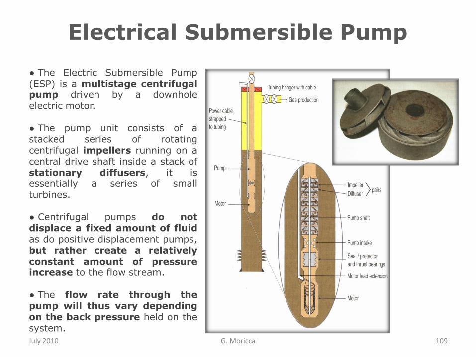
Electrical Submersible Pump
July 2010 G. Moricca 109
● The Electric Submersible Pump(ESP) is a multistage centrifugalpump driven by a downholeelectric motor.
● The pump unit consists of astacked series of rotatingcentrifugal impellers running on acentral drive shaft inside a stack ofstationary diffusers, it isessentially a series of smallturbines.
● Centrifugal pumps do notdisplace a fixed amount of fluidas do positive displacement pumps,but rather create a relativelyconstant amount of pressureincrease to the flow stream.
● The flow rate through thepump will thus vary dependingon the back pressure held on thesystem.

July 2010 G. Moricca 110
● The necessary rate and pressure to lift liquidsto surface are determined by the type andnumber of pump stages.
● The ESP is run in hole suspended to theproduction tubing. Therefore, if the downholeunit should fail, the tubing and pump should bepulled out together for repairs.
● Electric power is supplied to the motor by aprotected round or, in the case of limitedspace, flat cable unrolled along the outside ofthe tubing.
Electrical Submersible Pump

July 2010 G. Moricca 111
Advantages
● Preferred method for wells with:– Low gas oil ratio– High productivity index
● High water cut is not a restriction
● Can lift extremely high volume
● Flexibility: can handle rates from50 to 60.000 bpd
● Controllable production rate
● Comprehensive down-hole measurement
● Real time pump and well performance monitoring
● Can pump against high flow-tubinghead pressure
● Quick restart after shut down
● Long run pump life possible
Disadvantages
● Not applicable in case of:– High GOR– Sand production
● Tubing has to be pulled to replace the pump
● High cost for repairs, especially offshore
● High voltage (1000 V) electrical poweris required
● Susceptible to damage during completion
● No suitable for low volume wells: <150 BPD
● Power cable requires penetration of head and packer integrity
● Viscous crude reduce pump efficiency
● High temperature can degrade the electrical motor
Electrical Submersible Pump

Hydraulic Submersible Pump
July 2010 G. Moricca 112
Hydraulic pumps use a high pressure power fluid
pumped from the surface which :
● Drives a downhole, positive displacement pumps
● Powers a centrifugal or turbine pump
● Creates a reduced pressure by passage through
a venturi or nozzle where pressure energy is
converted into velocity
–This high velocity/low pressure flow of
the power fluid commingles with the
production flow in the throat of the pump.
–A diffuser reduces the velocity, increasing
the fluid pressure and allowing the
combined fluid to flow to surface
– The power fluid consists of oil or
production water
– The power fluid is supplied to the
downhole equipment via a separate
injection tubing
● The majority of installations commingle
the exhaust fluid with the production fluid through
the casing-tubing annulus

July 2010 G. Moricca 113
Advantages
● Range of application opportunities:― Small diameter wells not suited to
other Artificial lift methods― Tough retrofit completion and tough
liquid applications― As good alternative to the ESP
● The pump operate at higher speedthan an ESP (around three-four timeshigher revolution/min) therefore theyrequire few stages and are smaller
● No electrical connections or down-holeelectronics
● Flexibility: can handle rates from50 to 20.000 bpd
● Simple to operate: speed control by thevariation of supplied power fluid
● The power source can be remote from the wellhead giving a low wellhead profile attractive for offshore locations
● The power fluid can be commingled or returned in a separate conduit or disposed of down-hole
Disadvantages
● Pumps with moving parts have a short run life when supplied with poor quality power fluid. Solid-free power fluid is mandatory
● Commingle power-produced fluid imply:― power-produced fluids compatibility― power-produced fluids separation
● High GOR represent gas handling problems
● Viscous crude reduce pump efficiency
Hydraulic Submersible Pump
Jet Pump
July 2010 G. Moricca 114
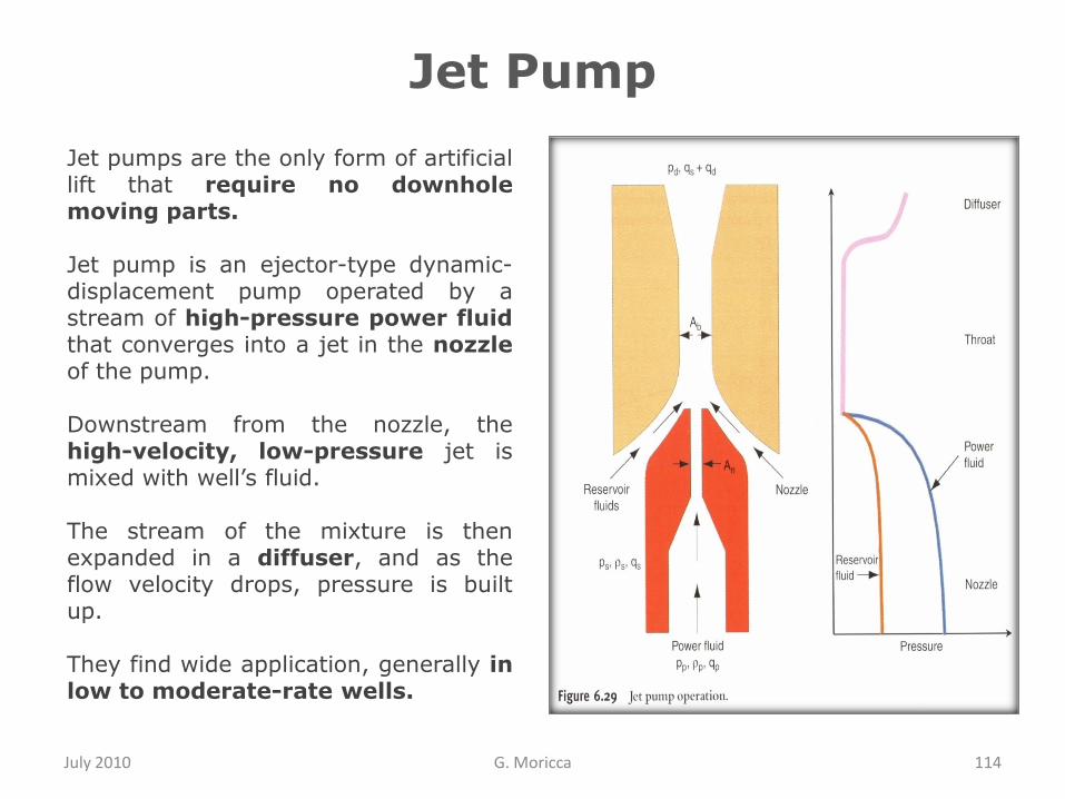
Jet pumps are the only form of artificiallift that require no downholemoving parts.
Jet pump is an ejector-type dynamic-displacement pump operated by astream of high-pressure power fluidthat converges into a jet in the nozzleof the pump.
Downstream from the nozzle, thehigh-velocity, low-pressure jet ismixed with well‟s fluid.
The stream of the mixture is thenexpanded in a diffuser, and as theflow velocity drops, pressure is builtup.
They find wide application, generally inlow to moderate-rate wells.

Jet Pump well configuration
July 2010 G. Moricca 115
Jet Pump
July 2010 G. Moricca 116
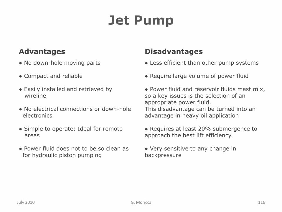
Advantages
● No down-hole moving parts
● Compact and reliable
● Easily installed and retrieved bywireline
● No electrical connections or down-holeelectronics
● Simple to operate: Ideal for remote areas
● Power fluid does not to be so clean asfor hydraulic piston pumping
Disadvantages
● Less efficient than other pump systems
● Require large volume of power fluid
● Power fluid and reservoir fluids mast mix, so a key issues is the selection of an appropriate power fluid.This disadvantage can be turned into an advantage in heavy oil application
● Requires at least 20% submergence to approach the best lift efficiency.
● Very sensitive to any change in backpressure
Progressive Cavity Pump
July 2010 G. Moricca 117
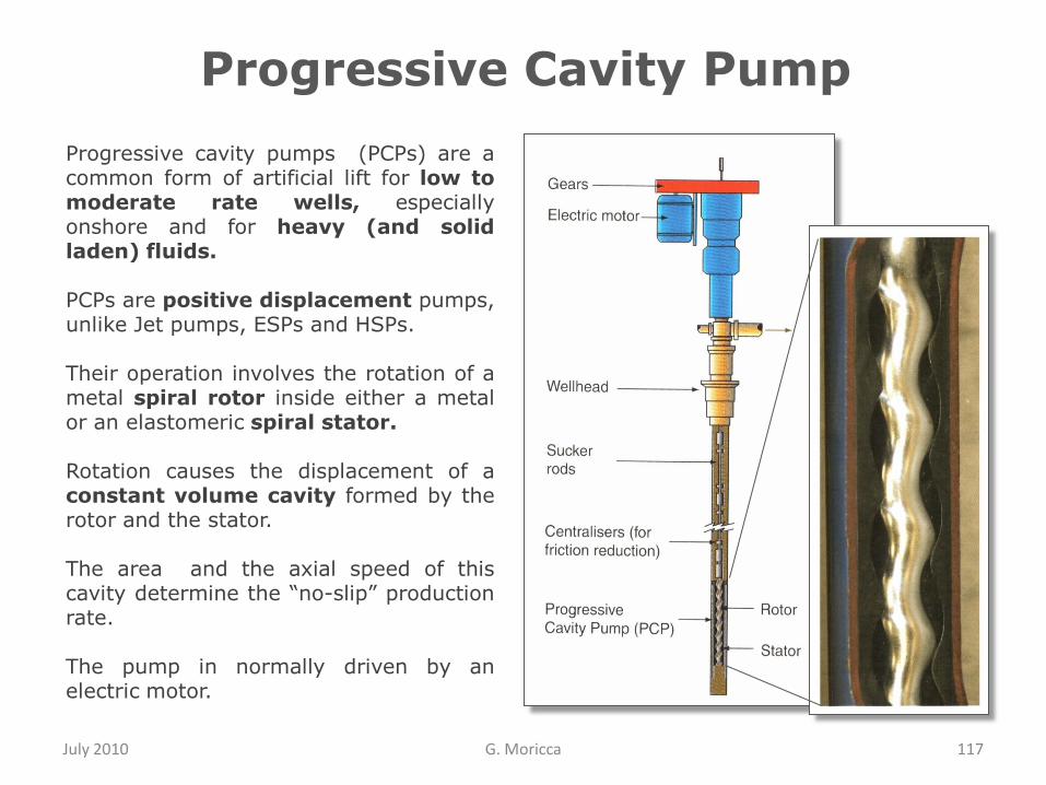
Progressive cavity pumps (PCPs) are acommon form of artificial lift for low tomoderate rate wells, especiallyonshore and for heavy (and solidladen) fluids.
PCPs are positive displacement pumps,unlike Jet pumps, ESPs and HSPs.
Their operation involves the rotation of ametal spiral rotor inside either a metalor an elastomeric spiral stator.
Rotation causes the displacement of aconstant volume cavity formed by therotor and the stator.
The area and the axial speed of thiscavity determine the “no-slip” productionrate.
The pump in normally driven by anelectric motor.
July 2010 G. Moricca 118
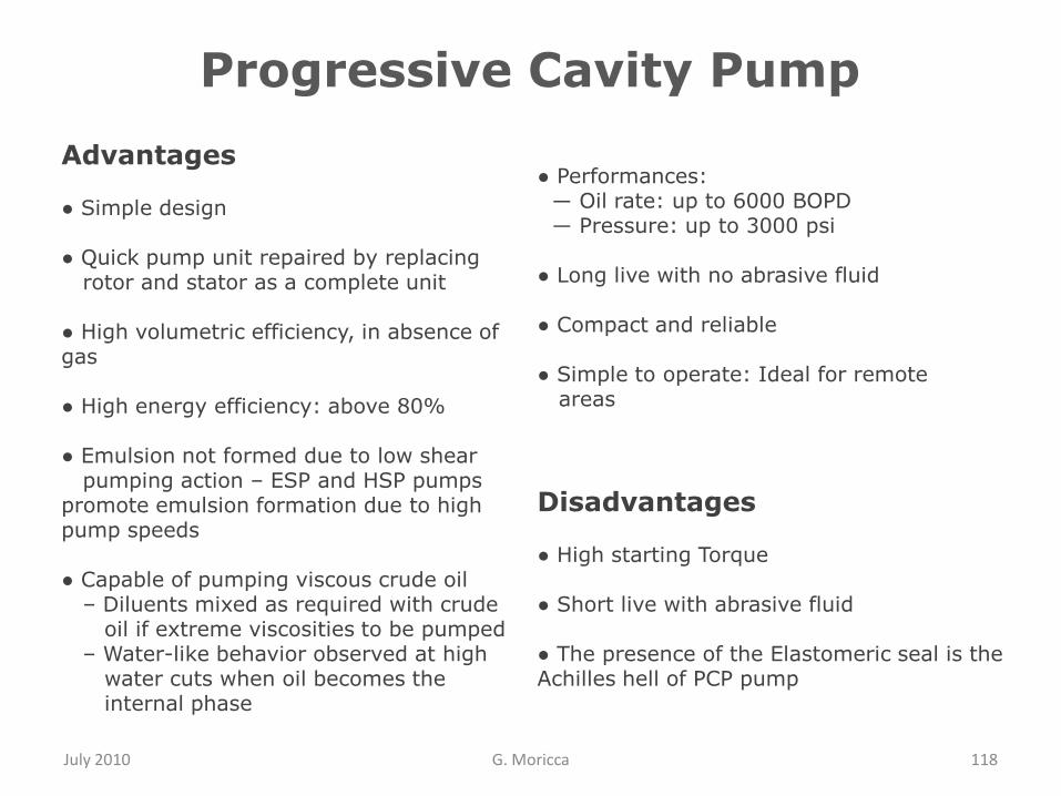
Advantages
● Simple design
● Quick pump unit repaired by replacingrotor and stator as a complete unit
● High volumetric efficiency, in absence of gas
● High energy efficiency: above 80%
● Emulsion not formed due to low shearpumping action – ESP and HSP pumps
promote emulsion formation due to high pump speeds
● Capable of pumping viscous crude oil– Diluents mixed as required with crude
oil if extreme viscosities to be pumped– Water-like behavior observed at high
water cuts when oil becomes theinternal phase
● Performances:― Oil rate: up to 6000 BOPD ― Pressure: up to 3000 psi
● Long live with no abrasive fluid
● Compact and reliable
● Simple to operate: Ideal for remote areas
Disadvantages
● High starting Torque
● Short live with abrasive fluid
● The presence of the Elastomeric seal is the Achilles hell of PCP pump
Progressive Cavity Pump
Beam or Sucker Rod Pump
July 2010 G. Moricca 119
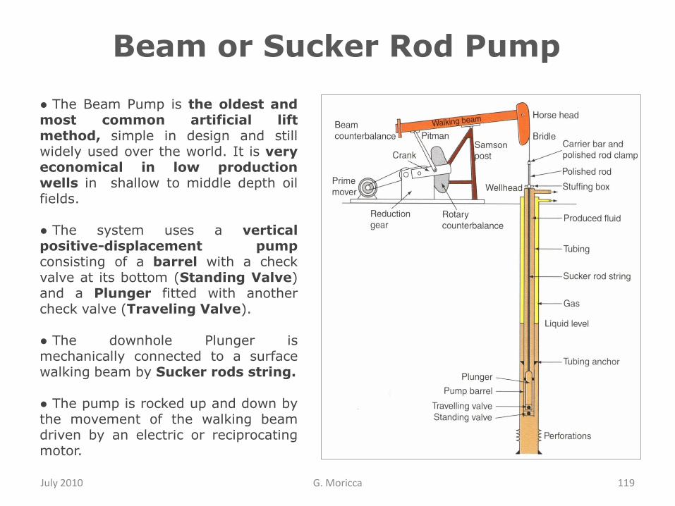
● The Beam Pump is the oldest andmost common artificial liftmethod, simple in design and stillwidely used over the world. It is veryeconomical in low productionwells in shallow to middle depth oilfields.
● The system uses a verticalpositive-displacement pumpconsisting of a barrel with a checkvalve at its bottom (Standing Valve)and a Plunger fitted with anothercheck valve (Traveling Valve).
● The downhole Plunger ismechanically connected to a surfacewalking beam by Sucker rods string.
● The pump is rocked up and down bythe movement of the walking beamdriven by an electric or reciprocatingmotor.
July 2010 G. Moricca 120
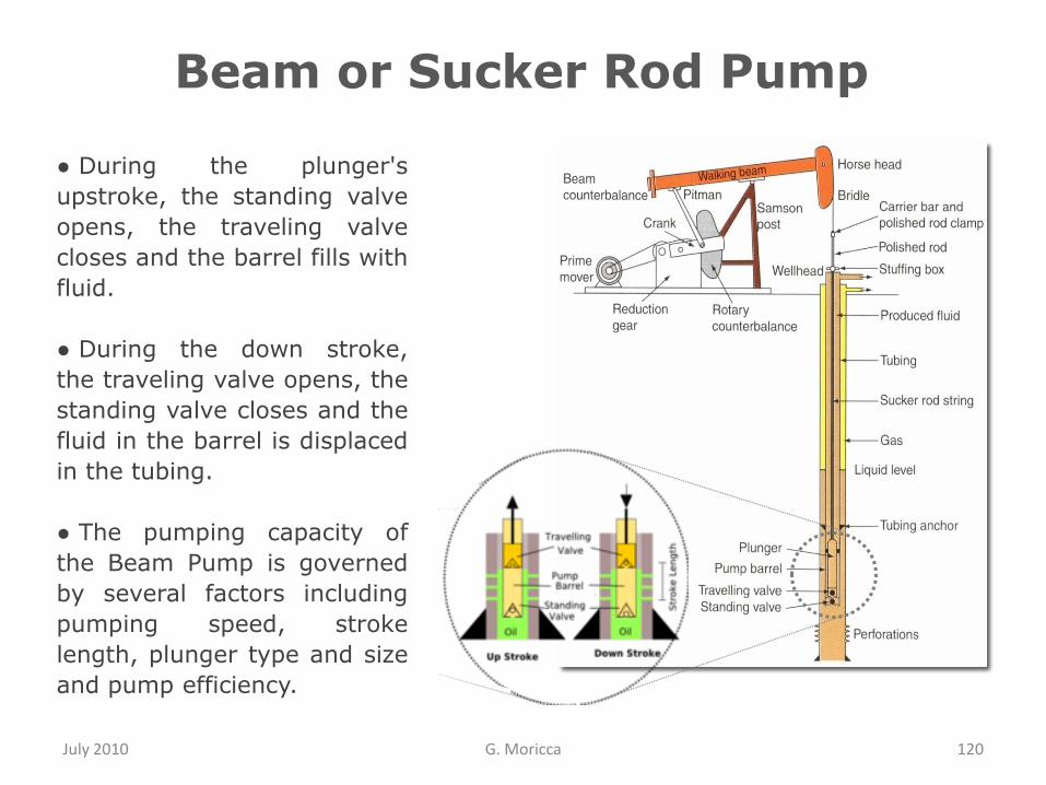
● During the plunger's
upstroke, the standing valve
opens, the traveling valve
closes and the barrel fills with
fluid.
● During the down stroke,
the traveling valve opens, the
standing valve closes and the
fluid in the barrel is displaced
in the tubing.
● The pumping capacity of
the Beam Pump is governed
by several factors including
pumping speed, stroke
length, plunger type and size
and pump efficiency.
Beam or Sucker Rod Pump
July 2010 G. Moricca 121
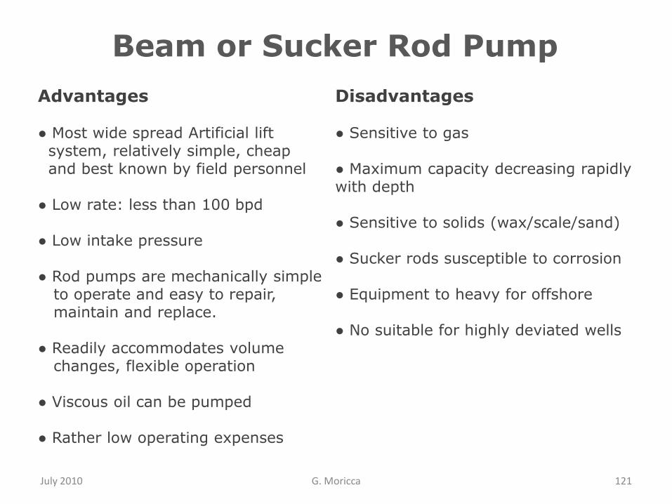
Advantages
● Most wide spread Artificial liftsystem, relatively simple, cheapand best known by field personnel
● Low rate: less than 100 bpd
● Low intake pressure
● Rod pumps are mechanically simpleto operate and easy to repair, maintain and replace.
● Readily accommodates volumechanges, flexible operation
● Viscous oil can be pumped
● Rather low operating expenses
Disadvantages
● Sensitive to gas
● Maximum capacity decreasing rapidly with depth
● Sensitive to solids (wax/scale/sand)
● Sucker rods susceptible to corrosion
● Equipment to heavy for offshore
● No suitable for highly deviated wells
Beam or Sucker Rod Pump
Artificial Lift System Selection
July 2010 G. Moricca 122
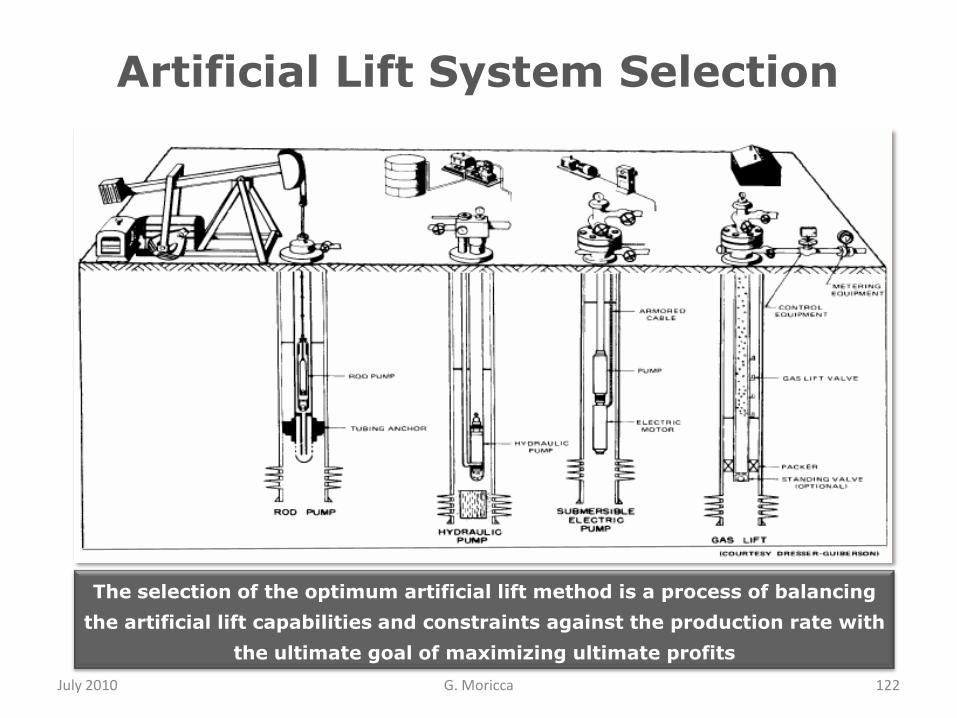
The selection of the optimum artificial lift method is a process of balancing
the artificial lift capabilities and constraints against the production rate with
the ultimate goal of maximizing ultimate profits

July 2010 G. Moricca 123
The main factors governing selection of artificial lift methods are:1. Production rate to be achieved2. Down-hole flowing pressure3. Gas-liquid ratio4. PVT producing fluid characteristics
The other factors to be considered are:
● Operating conditions― Casing size limitation― Well depth― Intake capabilities ( minimum bottom hole flowing pressure)― Flexibility of the artificial lift system― Surveillance― Testing, and time cycle or pump off controllers
● Well conditions― Corrosion/ scale-handling ability― Solids/sand handling ability― Temperature limitation― High-viscosity fluid handling― High and low –volume lift capabilities.
Cont/…
Artificial Lift System Selection
July 2010 G. Moricca 124
● Situation (new field discovery , new well , existing well ):― Many choices may be available for a new field discovery, for which
constraints can be minimized by the production facilities and well design.
― A new well in an exiting field is constrained by the existinginfrastructure: choices become limited.
― An existing well has many fixed constraints (completion, well integrity, location accessibility, etc) that minimize lift selection possibilities.
The original field development plan should address all known constraints and consider future changes (depletion, GOR, water cut) to the lift method.
As a result of the above considerations, the type of artificial lift system should be selected:1. Positive displacement pumps (PCP, Sucker Rod, Reciprocating Hydraulic
pump)2. Dynamic displacement pumps (ESP, HSP, Jet pump)3. Gas lift
Cont/...
Artificial Lift System Selection

July 2010 G. Moricca 125
Based on reservoir production performance analysis, two different approaches
should be investigated:
Long term
Short term
Long term
This frequently leads to the installation of oversized equipment in the
anticipation of ultimately producing large quantities of water. As a result, the
equipment may have operated at poor efficiency due to under-loading over a
significant portion of its total life.
Short term
Essentially, to design for what the well is producing today and not worry
about tomorrow. This can lead to many changes in the type of lift
equipment installed during the well‟s production life. Low cost operations may
result in the short term, but large sum of money will have to be spent later
on to change the artificial lift equipment and /or the completion.
Artificial Lift System Selection

ESP System
-
Quick-look of
Subsurface Components
July 2010 G. Moricca 126
July 2010 G. Moricca 127
Electric Submersible CentrifugalPump System
At the end of this section, you will be able to
understand the basic of ESP System Subsurface main
components:
Electric motor
Protector
Pump Intake
Pump
Cable
July 2010 G. Moricca 128
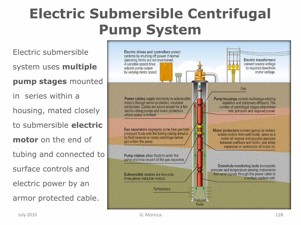
Electric submersible
system uses multiple
pump stages mounted
in series within a
housing, mated closely
to submersible electric
motor on the end of
tubing and connected to
surface controls and
electric power by an
armor protected cable.
Electric Submersible CentrifugalPump System
July 2010 G. Moricca 129
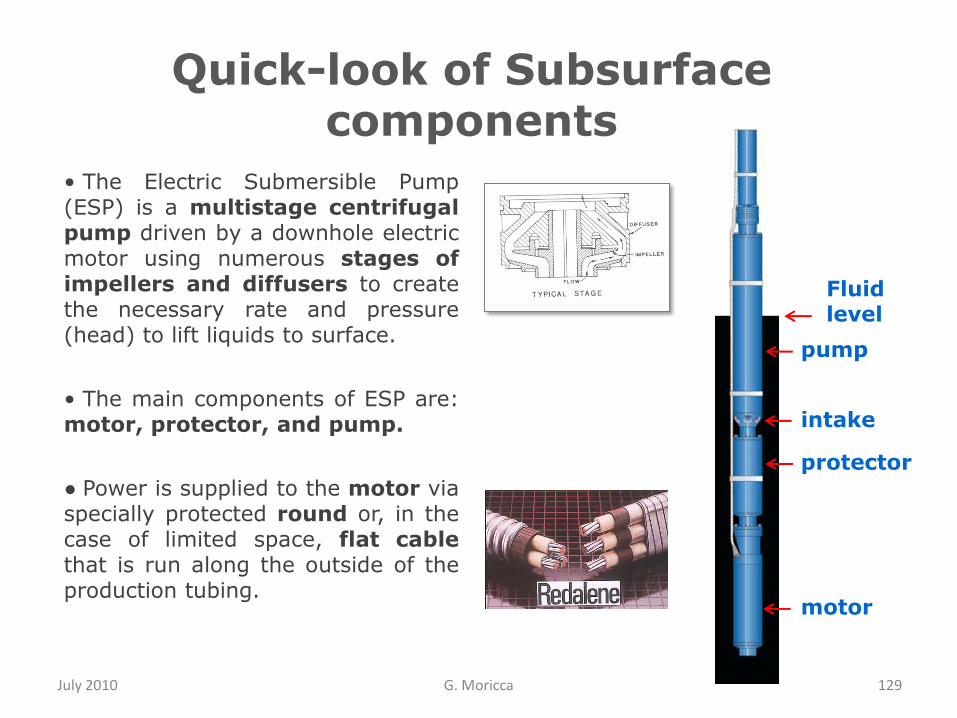
• The Electric Submersible Pump(ESP) is a multistage centrifugalpump driven by a downhole electricmotor using numerous stages ofimpellers and diffusers to createthe necessary rate and pressure(head) to lift liquids to surface.
• The main components of ESP are:motor, protector, and pump.
● Power is supplied to the motor viaspecially protected round or, in thecase of limited space, flat cablethat is run along the outside of theproduction tubing.
Quick-look of Subsurface components
motor
pump
protector
intake
Fluidlevel
July 2010 G. Moricca 130
Quick-look of Subsurface Components
ESP
Electric
Motor
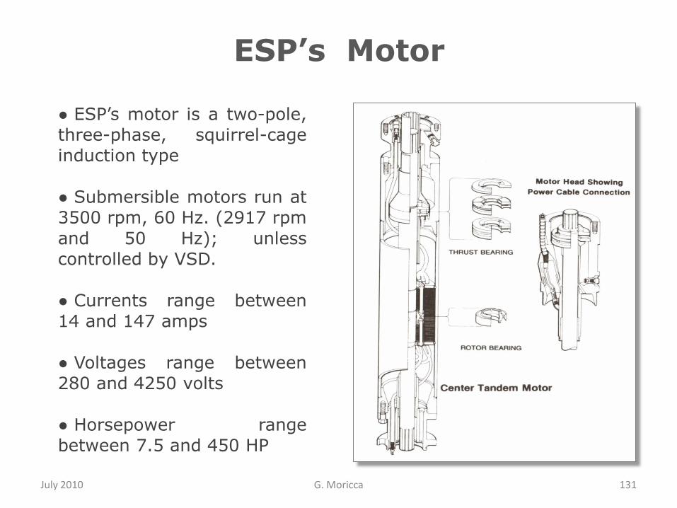
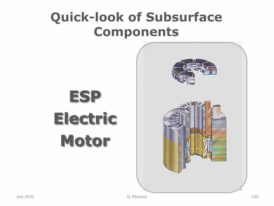
● ESP‟s motor is a two-pole,
three-phase, squirrel-cage
induction type
● Submersible motors run at
3500 rpm, 60 Hz. (2917 rpm
and 50 Hz); unless
controlled by VSD.
● Currents range between
14 and 147 amps
● Voltages range between
280 and 4250 volts
● Horsepower range
between 7.5 and 450 HP
July 2010 G. Moricca 131
ESP’s Motor
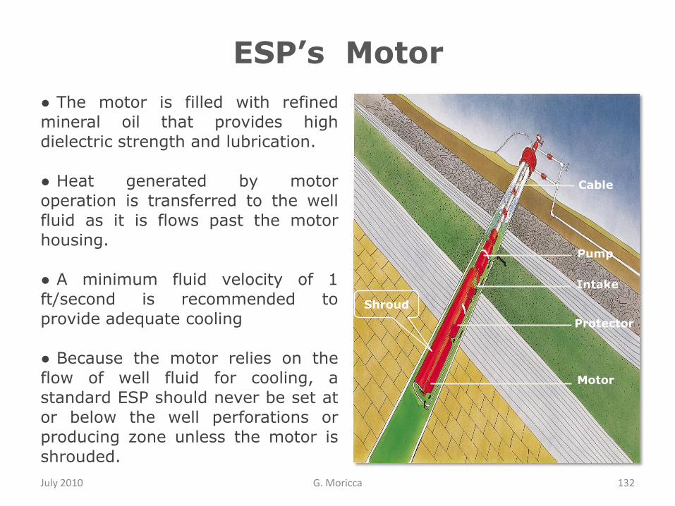
● The motor is filled with refined
mineral oil that provides high
dielectric strength and lubrication.
● Heat generated by motor
operation is transferred to the well
fluid as it is flows past the motor
housing.
● A minimum fluid velocity of 1
ft/second is recommended to
provide adequate cooling
● Because the motor relies on the
flow of well fluid for cooling, a
standard ESP should never be set at
or below the well perforations or
producing zone unless the motor is
shrouded.
July 2010 G. Moricca 132
ESP’s Motor
Cable
Pump
Intake
Protector
Motor
Shroud
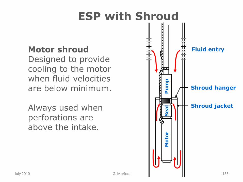
July 2010 G. Moricca 133
Seal
Mo
tor
Pu
mp
Shroud jacket
Shroud hanger
Fluid entryMotor shroud Designed to provide cooling to the motor when fluid velocities are below minimum.
Always used when perforations are above the intake.
ESP with Shroud

July 2010 G. Moricca 134
ESP’sMotor
Protector

July 2010 G. Moricca 135
The protector
is the piece
of equipment
that is
typically
placed above
the motor.
ESP’s Protector

The protector performs the following
basic functions:
● Connects the pump to the motor
● Provides the thrust bearing that
carries the pump thrust load.
● Prevents entry of well fluids into the
motor.
● Equalizes pressures between the
motor and the wellbore.
● Allows thermal expansion of the
motor oil resulting from operating heat
and motor oil contraction after
shutdown.
July 2010 G. Moricca 136
ESP’s Motor Protector
Mechanical
seal
Thrust
bearing
component
July 2010 G. Moricca 137
ESP’s Pump Intake
-Standard Intake
and
Gas Separator Intake
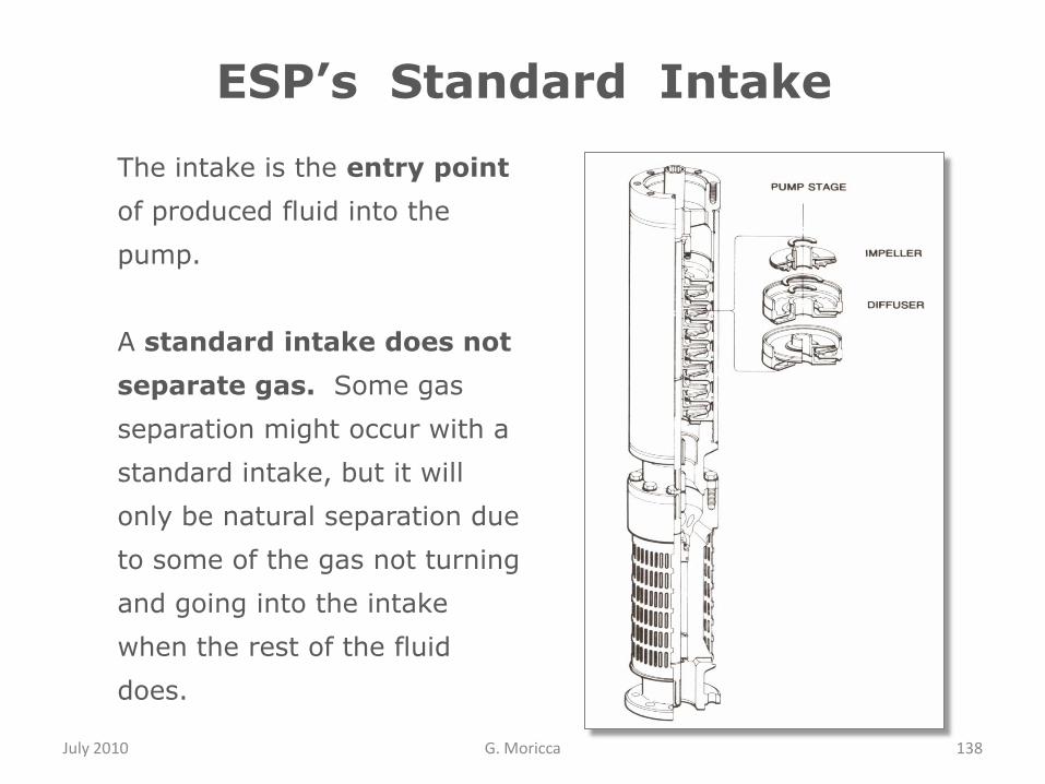
July 2010 G. Moricca 138
Bolt-on Intake
The intake is the entry point
of produced fluid into the
pump.
A standard intake does not
separate gas. Some gas
separation might occur with a
standard intake, but it will
only be natural separation due
to some of the gas not turning
and going into the intake
when the rest of the fluid
does.
ESP’s Standard Intake

July 2010 G. Moricca 139
ESP’s Gas Separator
A Gas Separator intake is used when the gas/liquid ratio (GLR) is greater than can be handled by the pump.
If the gas remains in solution, the pump will perform normally.Once the free gas increases, the pump will eventually “gas lock” which drastically reduces fluid production and in extreme cases can damage the pump.
There are two types of gas separator:● Static● Rotary
Staticseparator
Dynamicseparator
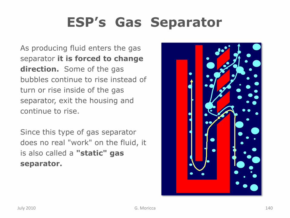
July 2010 G. Moricca 140
Bolt-on Intake
As producing fluid enters the gas
separator it is forced to change
direction. Some of the gas
bubbles continue to rise instead of
turn or rise inside of the gas
separator, exit the housing and
continue to rise.
Since this type of gas separator
does no real "work" on the fluid, it
is also called a "static" gas
separator.
ESP’s Gas Separator

July 2010 G. Moricca 141
ESP’s Rotary Gas Separator
The rotary gas separator design
works in a similar fashion to a
centrifuge. The centrifuge
"paddles" spinning at 3500 rpm
cause the heavier fluids to be
forced to the outside, through
the crossover and up into the
pump, while the lighter fluid
(vapor) stays toward the
center, and exits through the
crossover and discharge ports
back into the well.

July 2010 G. Moricca 142
Subsurface
Electrical
Centrifugal Pump
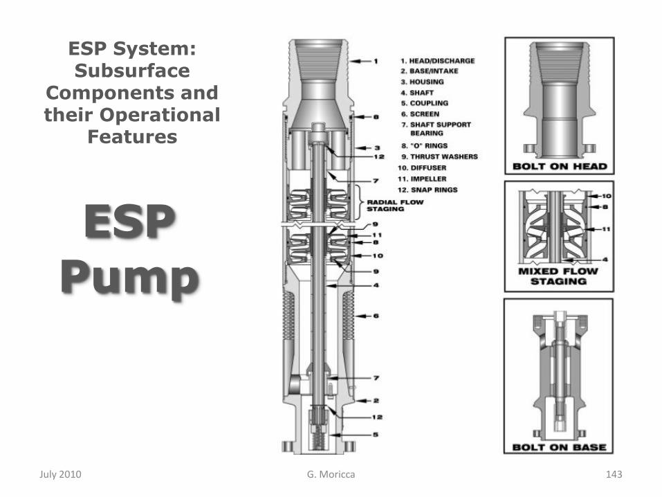
July 2010 143G. Moricca
ESP
Pump
ESP System: Subsurface
Components and their Operational
Features
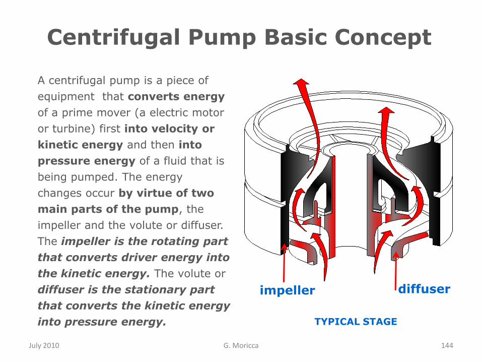
July 2010 G. Moricca 144
Centrifugal Pump Basic Concept
A centrifugal pump is a piece of
equipment that converts energy
of a prime mover (a electric motor
or turbine) first into velocity or
kinetic energy and then into
pressure energy of a fluid that is
being pumped. The energy
changes occur by virtue of two
main parts of the pump, the
impeller and the volute or diffuser.
The impeller is the rotating part
that converts driver energy into
the kinetic energy. The volute or
diffuser is the stationary part
that converts the kinetic energy
into pressure energy. TYPICAL STAGE
impeller diffuser

ESP’s Impeller
July 2010 G. Moricca 145
As liquid leaves the eye of the impeller a low-pressure area is created causing more liquid to flow toward the inlet. Because the impeller blades are curved, the fluid is pushed in a tangential and radial direction by the centrifugal force.
This force acting inside the pump is the same one that keeps water inside a bucket that is rotating at the end of a string.
The liquid enters into center (eye) of a revolving device (impeller). When the impeller rotates, it spins the liquid outward and provides centrifugal acceleration.
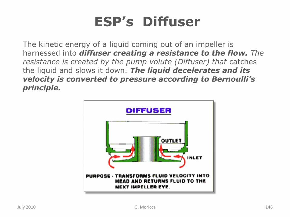
ESP’s Diffuser
July 2010 G. Moricca 146
The kinetic energy of a liquid coming out of an impeller is harnessed into diffuser creating a resistance to the flow. The resistance is created by the pump volute (Diffuser) that catches the liquid and slows it down. The liquid decelerates and its velocity is converted to pressure according to Bernoulli’s principle.
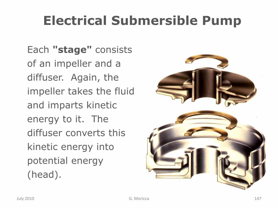
Electrical Submersible Pump
July 2010 G. Moricca 147
Each "stage" consists
of an impeller and a
diffuser. Again, the
impeller takes the fluid
and imparts kinetic
energy to it. The
diffuser converts this
kinetic energy into
potential energy
(head).
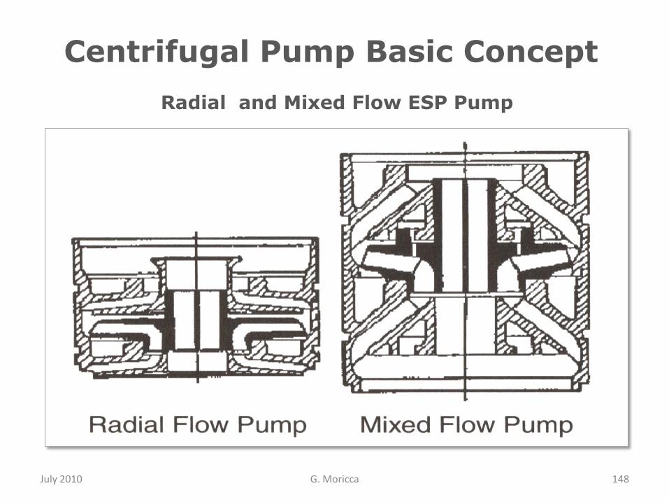
July 2010 G. Moricca 148
Centrifugal Pump Basic Concept
Radial and Mixed Flow ESP Pump

July 2010 G. Moricca 149
Centrifugal Pump Basic Concept
Radial Flow ESP Pump
Radial flow pumps have
low specific speed
and develop their head
mostly due to the
conversion of centrifugal
forces.
The specific speed is defined as: The rotational speed (RPM) required to produce a liquid rate of 1 gallon per minute against 1 ft of head.

July 2010 G. Moricca 150
Centrifugal Pump Basic Concept
Mixed Flow ESP Pump
Mixed flow pumps have high
specific speed and operate
only partially on centrifugal
force and more and more of
the total head is developed by
the lifting action of the
impellers.
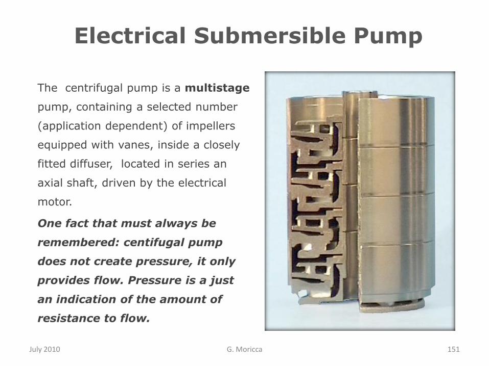
Electrical Submersible Pump
July 2010 G. Moricca 151
The centrifugal pump is a multistage
pump, containing a selected number
(application dependent) of impellers
equipped with vanes, inside a closely
fitted diffuser, located in series an
axial shaft, driven by the electrical
motor.
One fact that must always be
remembered: centifugal pump
does not create pressure, it only
provides flow. Pressure is a just
an indication of the amount of
resistance to flow.

July 2010 G. Moricca 152
ESP’sPower Cable
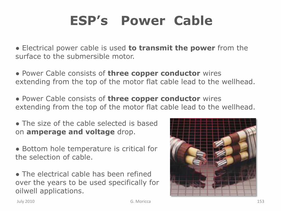
ESP’s Power Cable
July 2010 G. Moricca 153
● Electrical power cable is used to transmit the power from the surface to the submersible motor.
● Power Cable consists of three copper conductor wires extending from the top of the motor flat cable lead to the wellhead.
● Power Cable consists of three copper conductor wires extending from the top of the motor flat cable lead to the wellhead.
● The size of the cable selected is based on amperage and voltage drop.
● Bottom hole temperature is critical for the selection of cable.
● The electrical cable has been refined over the years to be used specifically for oilwell applications.
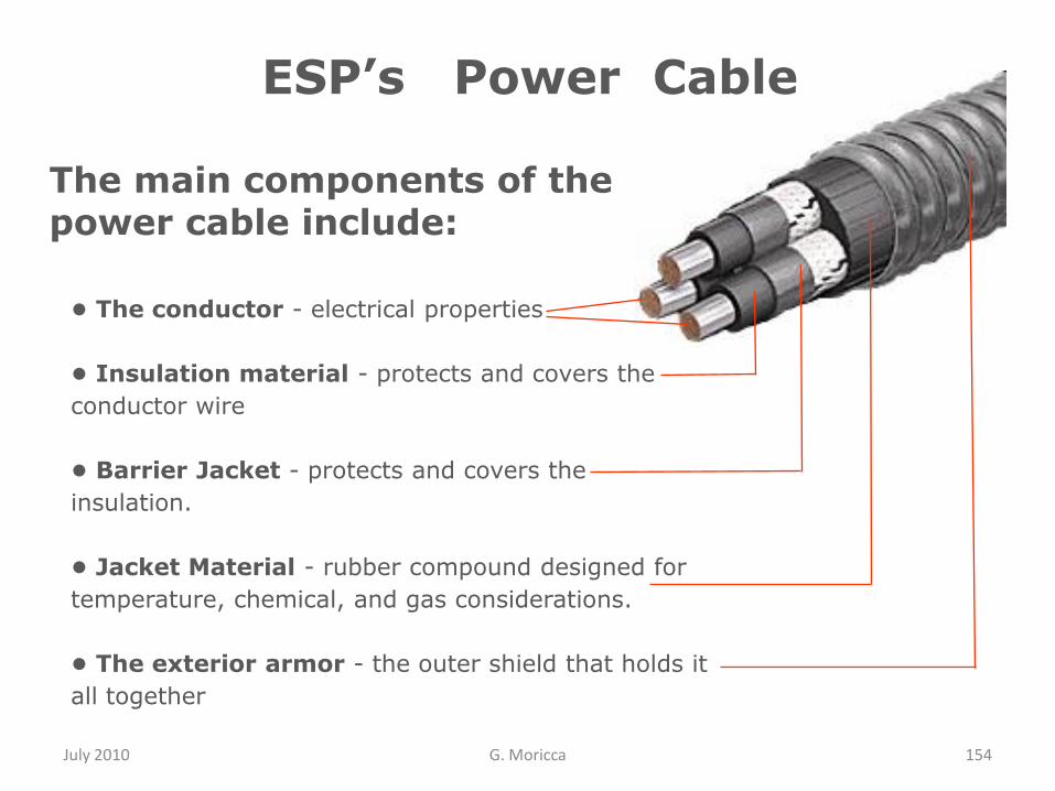
July 2010 G. Moricca 154
● The conductor - electrical properties
● Insulation material - protects and covers the
conductor wire
● Barrier Jacket - protects and covers the
insulation.
● Jacket Material - rubber compound designed for
temperature, chemical, and gas considerations.
● The exterior armor - the outer shield that holds it
all together
The main components of the power cable include:
ESP’s Power Cable

ESP System
-
ESP Pump
Performance
Curves
July 2010 G. Moricca 155
July 2010 G. Moricca 156
Electric Submersible CentrifugalPump
At the end of this section, you will be able to:
― Understand the ESP Performance curves:
− pumping Head
− pumping Power
− pump Efficiency
― Use the ESP Performance curves
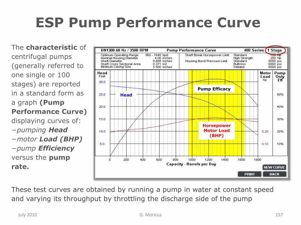
ESP Pump Performance Curve
July 2010 G. Moricca 157
The characteristic of
centrifugal pumps
(generally referred to
one single or 100
stages) are reported
in a standard form as
a graph (Pump
Performance Curve)
displaying curves of:
−pumping Head
−motor Load (BHP)
−pump Efficiency
versus the pump
rate.
HorsepowerMotor Load
(BHP)
Head
Pump Efficacy
These test curves are obtained by running a pump in water at constant speed
and varying its throughput by throttling the discharge side of the pump
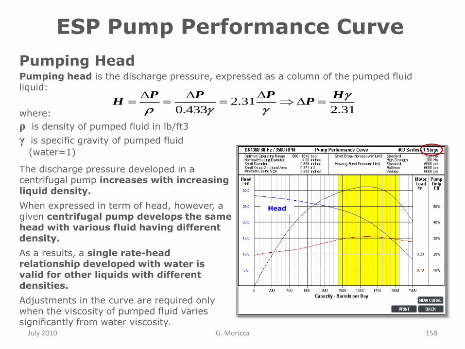
ESP Pump Performance Curve
July 2010 G. Moricca 158
Pumping HeadPumping head is the discharge pressure, expressed as a column of the pumped fluid liquid:
31.231.2
433.0
HP
PPPH
where:
ρ is density of pumped fluid in lb/ft3
γ is specific gravity of pumped fluid
(water=1)
The discharge pressure developed in a centrifugal pump increases with increasing liquid density.
When expressed in term of head, however, a given centrifugal pump develops the same head with various fluid having different density.
As a results, a single rate-head relationship developed with water is valid for other liquids with different densities.
Adjustments in the curve are required only when the viscosity of pumped fluid varies significantly from water viscosity.
Head
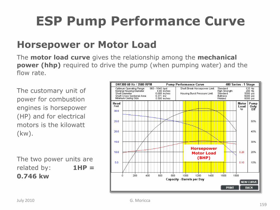
ESP Pump Performance Curve
July 2010 G. Moricca159
Horsepower or Motor Load
The motor load curve gives the relationship among the mechanical
power (hhp) required to drive the pump (when pumping water) and the
flow rate.
HorsepowerMotor Load
(BHP)
The customary unit of
power for combustion
engines is horsepower
(HP) and for electrical
motors is the kilowatt
(kw).
The two power units are
related by: 1HP =
0.746 kw
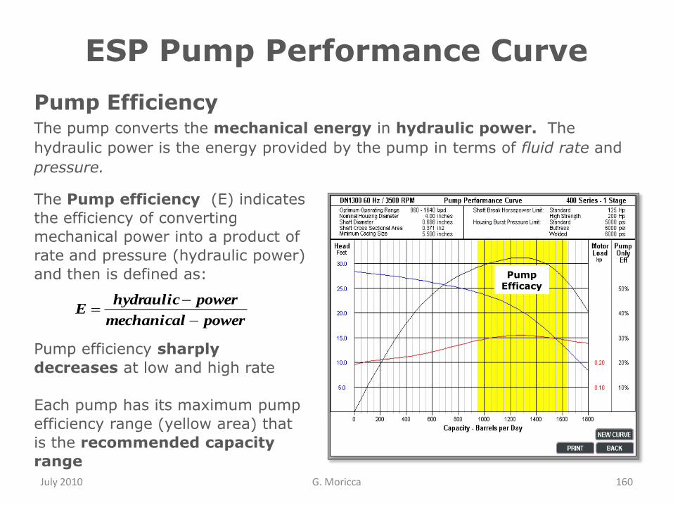
ESP Pump Performance Curve
July 2010 G. Moricca 160
The Pump efficiency (E) indicates
the efficiency of converting
mechanical power into a product of
rate and pressure (hydraulic power)
and then is defined as:
Pump efficiency sharply
decreases at low and high rate
Each pump has its maximum pump
efficiency range (yellow area) that
is the recommended capacity
range
powermechanical
powerhydraulicE
PumpEfficacy
Pump EfficiencyThe pump converts the mechanical energy in hydraulic power. The
hydraulic power is the energy provided by the pump in terms of fluid rate and
pressure.
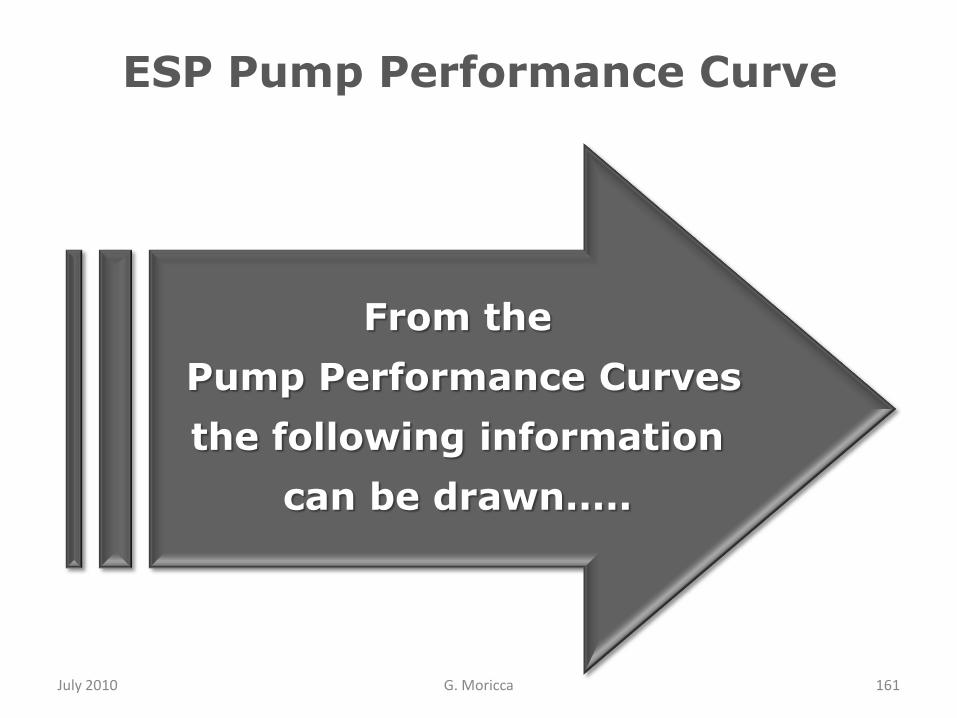
ESP Pump Performance Curve
July 2010 G. Moricca 161
From the
Pump Performance Curves
the following information
can be drawn.....

ESP Pump Performance Curve
July 2010 G. Moricca 162
If the motor
of DN13000
ESP is fed at
60Hz, it run at
constant rate
of 3500 RPM,
regarding-less
the pump fluid
rate and the
corresponding
head.
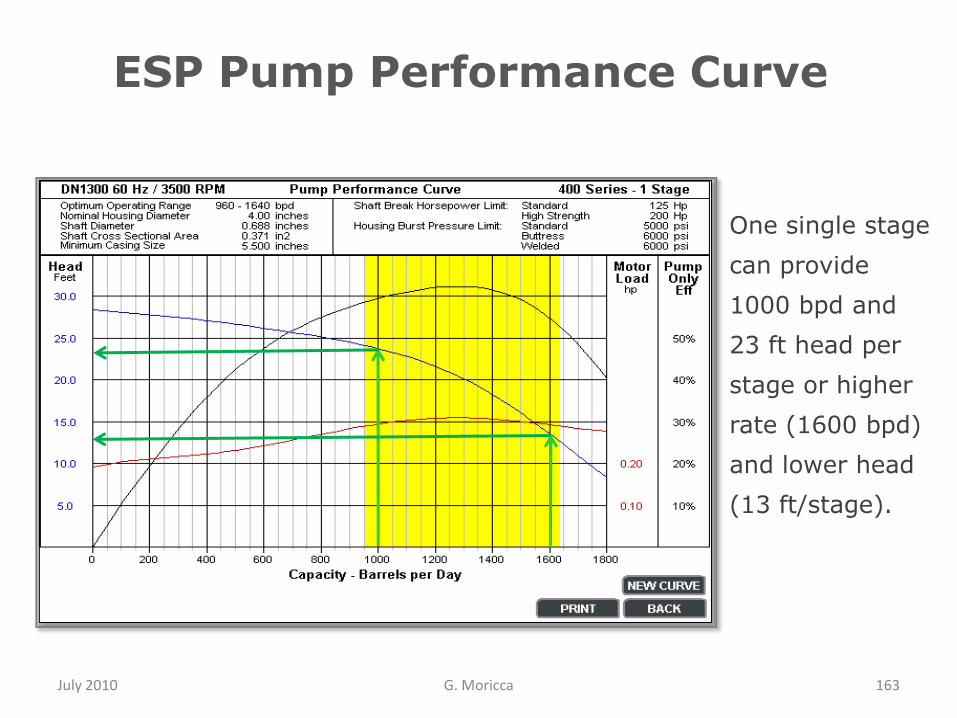
July 2010 G. Moricca 163
One single stage
can provide
1000 bpd and
23 ft head per
stage or higher
rate (1600 bpd)
and lower head
(13 ft/stage).
ESP Pump Performance Curve
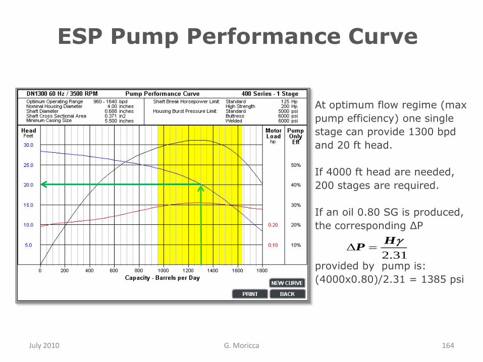
July 2010 G. Moricca 164
At optimum flow regime (max
pump efficiency) one single
stage can provide 1300 bpd
and 20 ft head.
If 4000 ft head are needed,
200 stages are required.
If an oil 0.80 SG is produced,
the corresponding ΔP
provided by pump is:
(4000x0.80)/2.31 = 1385 psi
31.2
HP
ESP Pump Performance Curve
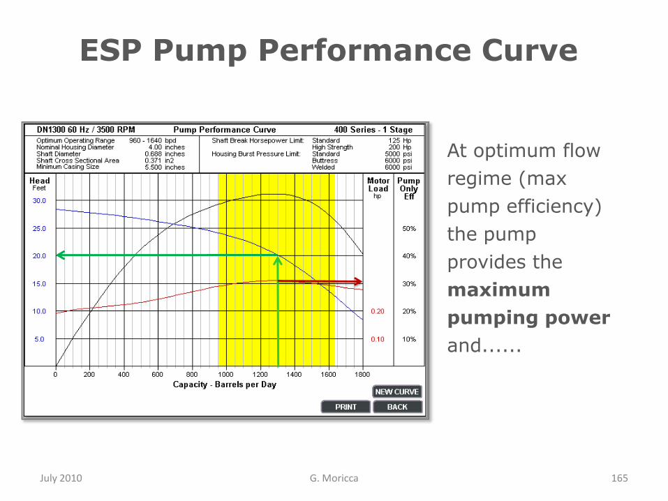
July 2010 G. Moricca 165
At optimum flow
regime (max
pump efficiency)
the pump
provides the
maximum
pumping power
and......
ESP Pump Performance Curve
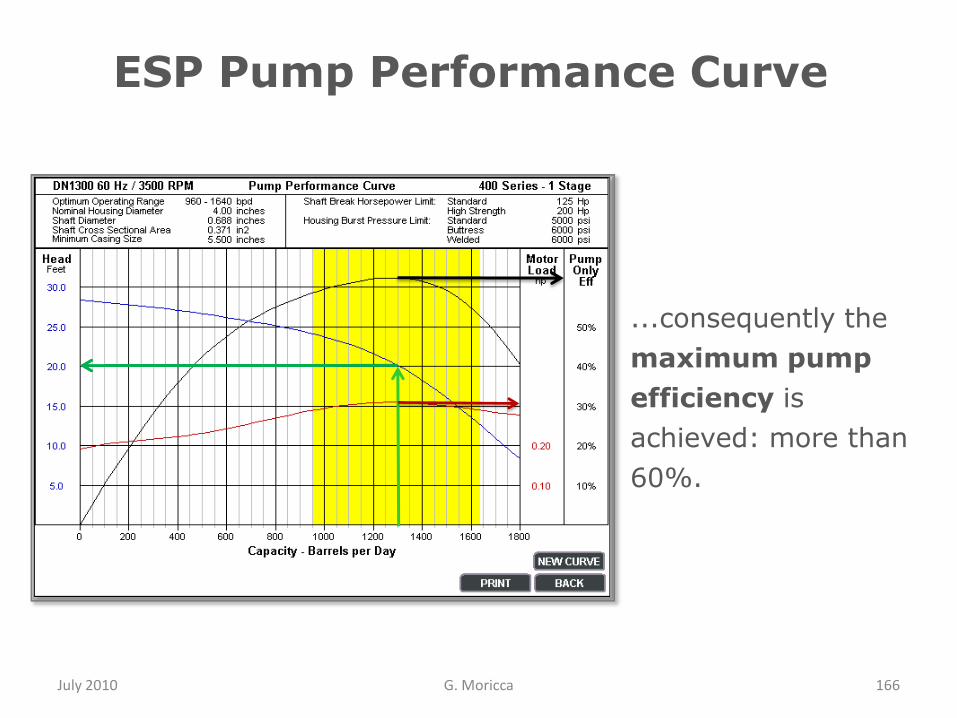
July 2010 G. Moricca 166
...consequently the
maximum pump
efficiency is
achieved: more than
60%.
ESP Pump Performance Curve
July 2010 G. Moricca 167
ESP System
-
Quick-look of Surface
Components

July 2010 G. Moricca 168
ESP System Surface Components
At the end of this section, you will be able to
understand the basic of ESP System Surface main
components:
Transformer
Switchboard/Motor Control devise
Junction box
Variable Speed Drive System

July 2010 G. Moricca 169
Quick-look of Surface Components
Perforations.
Protector
Pump intake
Pump
Joint Tubing
Check valveDrain valve
Casing
MotorPothead
Motor flat cable
Primary cable
Production
WellheadJunction
box
Motor
controller
Transformers
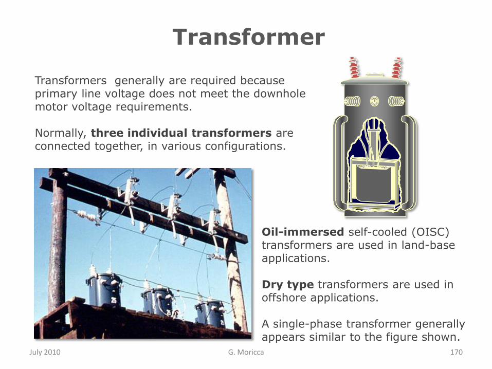
July 2010 G. Moricca 170
Transformers generally are required because primary line voltage does not meet the downhole motor voltage requirements.
Normally, three individual transformers are connected together, in various configurations.
Transformer
Oil-immersed self-cooled (OISC) transformers are used in land-base applications.
Dry type transformers are used in offshore applications.
A single-phase transformer generally appears similar to the figure shown.

July 2010 G. Moricca 171
Switchboard/Motor Controller
The switchboard is basically a motor control device.
Voltage capability ranges from 600 to 4.900 Volt on standard switchboards.
The switchboards range in complexity from a simple motor starter/disconnect switch to an extremely sophisticated monitoring/control device.
The purpose of motor controller is to protect the down-hole unit by sensing abnormal power service and shutting down the power supply.
The monitoring function applies to both overload and under-load conditions.
It can be programmed to automatically restart the down-hole motor following a user-selected time delay if the fault condition is caused by an under-load.
Overload condition shut-down must be restarted manually.This should be done only after the fault condition has been identified and corrected.
The controller also provides the capability to monitor the Production system with the use of a recording instrument.
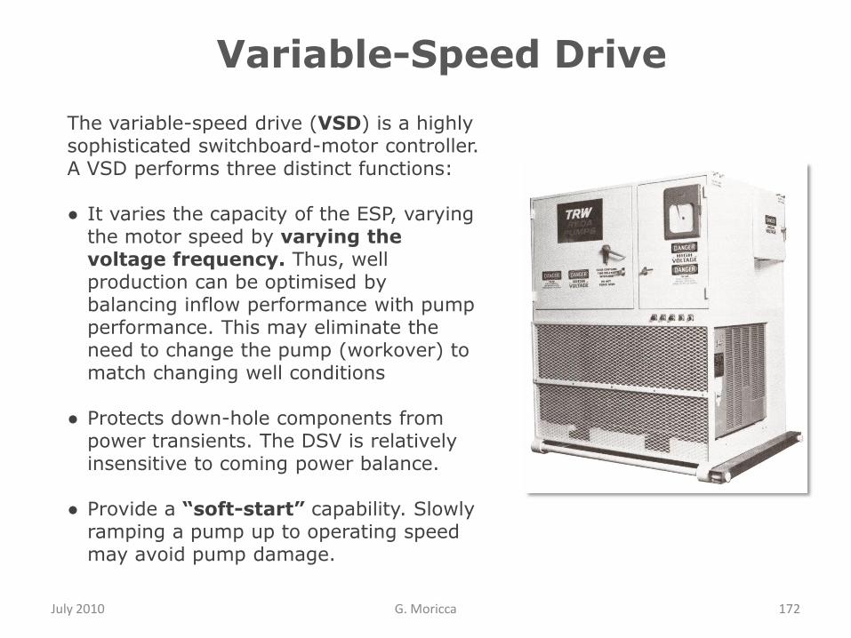
July 2010 G. Moricca 172
Variable-Speed Drive
The variable-speed drive (VSD) is a highly sophisticated switchboard-motor controller. A VSD performs three distinct functions:
● It varies the capacity of the ESP, varying the motor speed by varying the voltage frequency. Thus, well production can be optimised by balancing inflow performance with pump performance. This may eliminate the need to change the pump (workover) to match changing well conditions
● Protects down-hole components from power transients. The DSV is relatively insensitive to coming power balance.
● Provide a “soft-start” capability. Slowly ramping a pump up to operating speed may avoid pump damage.
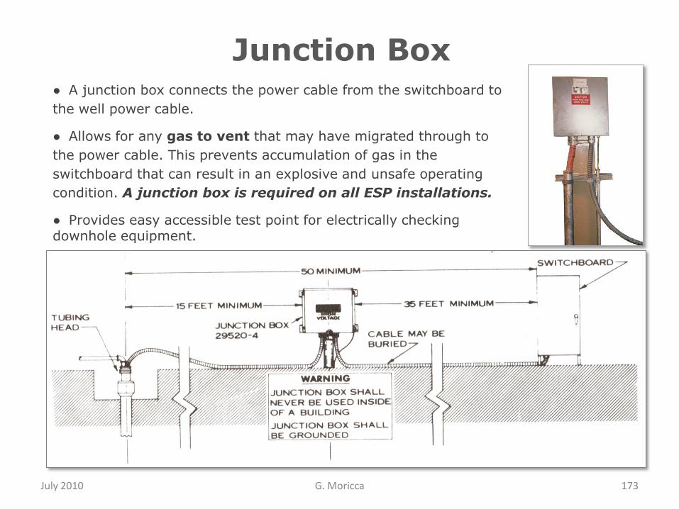
July 2010 G. Moricca 173
Junction Box● A junction box connects the power cable from the switchboard to
the well power cable.
● Allows for any gas to vent that may have migrated through to
the power cable. This prevents accumulation of gas in the
switchboard that can result in an explosive and unsafe operating
condition. A junction box is required on all ESP installations.
● Provides easy accessible test point for electrically checking downhole equipment.
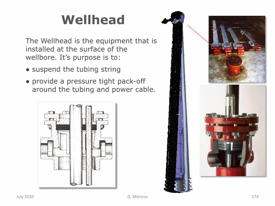
July 2010 G. Moricca 174
Wellhead
The Wellhead is the equipment that is installed at the surface of the wellbore. It‟s purpose is to:
● suspend the tubing string
● provide a pressure tight pack-off around the tubing and power cable.
July 2010 G. Moricca 175
ESP SystemsAbout 15 to 20 percent of almost one million wells worldwide
are pumped with some form of artificial lift employing electric
submersible pumps.
ESP systems are the fastest growing form of artificial lift pumping
technology. They are often considered high volume and depth
champions among oil field lift systems.
ESP systems can be used in casing as small as 4.5-in outside
diameter and can be engineered to handle contaminants commonly
found in oil-aggressive corrosive fluids such as H2S and CO2,
abrasive contaminants such as sand, exceptionally high
downhole temperatures and high levels of gas production.
Increasing water cut has been shown to have no significant
detrimental effect on ESP performance.
ESPs have been deployed in vertical, deviated and horizontal wells,
but they should be located in a straight section of casing for optimum
run life performance

July 2010 G. Moricca 176
ESP Artificial Lift Application Summary
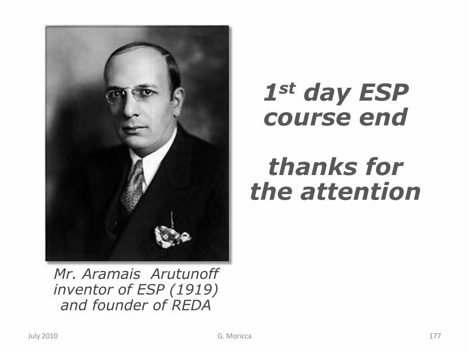
1st day ESP course end
thanks for the attention
July 2010 G. Moricca 177
Mr. Aramais Arutunoffinventor of ESP (1919) and founder of REDA


