32
Gretchen Greene, Ph.D. and Mark Rockel, Ph.D. Senior Natural Resource Economists, ENVIRON Overview of Ecosystem Services Quantification and Valuation Approaches

Gretchen Greene, Ph.D. and Mark Rockel, Ph.D.
Senior Natural Resource Economists, ENVIRON
Overview of Ecosystem
Services Quantification and
Valuation Approaches

Overview of Ecosystem Services
Quantification and Valuation Approaches
• Bringing the quantitative value of ecosystem
service changes into economic decision-making
• Separate Three Types of Activities:
– Taking Stock: Estimating Values for Entire Natural
Capital Stock – Environmental Accounting
– Creating Markets: Bringing more “nonmarket” goods
and services into the market system
– Evaluating Tradeoffs: Strategies that consider
marginal changes, and employ interdisciplinary teams
using a variety of different tools to make decisions that
impact the natural environment

Overview of Ecosystem Services
Quantification and Valuation Approaches
• Introduction
•Overview of Approach
•Examples
•Summary

Overview of Ecosystem Services
Quantification and Valuation Approaches
Introduction
• Framework
• Pros and Cons
• History
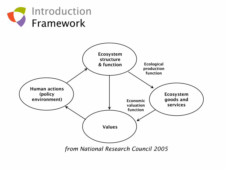
Economic
valuation
function
Ecological
production
function
Ecosystem
structure
& function
Values
Ecosystem
goods and
services
Human actions
(policy
environment)
from National Research Council 2005
Introduction
Framework

Introduction:
Framework – Economic Value Types
• Market Values
– Timber
– Commercial Fishing
– Agriculture
• Emerging Ecosystem
Service Markets
– Wetland Banks
– Carbon Markets
– Water Quality Trading
– Air Quality Markets
• Non-Market Values
– Direct Use
• Recreation
• Education
• Subsistence
– Indirect Use Value
• Habitat
• Flood Projection
– Passive Use Value
• Religious/Cultural
• Nonuse/Existence
Value
• Option

Introduction:
Framework – MEA Service Types

Introduction:
Framework – Valuation Techniques
• Travel cost method
• Hedonic pricing
• Contingent value/
choice/conjoint analysis
• Benefit transfer
• Averting behavior/
avoided cost
• Ecosystem service market
prices

Introduction
Pros and Cons of Valuing Ecosystem Services
• Case for
– Stewardship
– Manage assets/liabilities
– Public planning/investing
– Prevent damage/degradation
– Environmental accounting
– Establish payments for ecological services
• Case against
– Commodification of nature
– Difficult, lack of agreement
– May not work (may do more harm than good)
– Free market environmentalism

Introduction:
Economic Value History
• Travel cost suggested late 1940s
– Harold Hotelling recommends federal government use travel
costs as a proxy for the value of national parks to the nation
• Methods evolve through 1970s
– Travel Cost Method (TCM)
– Contingent Valuation Method (CVM)
– Hedonic Property Values
• Benefit cost analysis
(Principles & Guidelines) 1983
– Public decision making including values for improving/degrading
environmental quality
– Framework still used today (baseline, change from, monetary
value estimate for nonmarket goods)
• Free market environmentalism 1991

Introduction:
Economic Value History
• Environmental accounting 1990s
– Wasting Assets (Repetto et al., 1989)
– U.N. Recognizes need for “satellite”
system to the System of National
Accounts (SNA), 1993
• Valdez “blue ribbon panel” 1995
– Panel defines protocols for use and
application of different methodologies
like CVM
• Ecosystem services 2000 - ?
• Millennium assessment 2003
• Geo Spatial Modeling

Valuation of Ecosystem Services to Support
Decision-Making
Overview of Approach

Overview of Approach:
Ask Key Questions
• Goal of analysis
• Scale
– Geographic
– Demographic
– Temporal
• Gains, losses or status quo?
• Economic, ecologic or both?
• Ex-ante or ex-post?

Services (%
)
0%
100%
Pristine condition service level
Time →
Baseline service level given
anthropogenic sources/industrialization
Adverse impact
Net change in ecosystem services with
decline and rebound over time
Overview of Approach:
Establish Baseline

Overview of Approach:
Understand changes from baseline

Overview of Approach:
Evaluate with/without change
Figure 1. Three different payments for
environmental services scenarios: (a) static,
(b) deteriorating, and (c) improving service-
delivery baseline. Dotted lines show de facto
service delivered “with ES”; solid lines show
counterfactual baseline “without ES.”
Additionality is the incremental service
delivered through PES vis-`a-vis the
counterfactual baseline.
Wunder 2007

Overview of Approach:
Aggregate through time
Year Value
Compound/
Discount
Factor
Adjusted
Value
1997 $515,712 1.47 $757,341
1998 $537,844 1.43 $766,837
1999 $537,979 1.38 $744,689
2000 $548,262 1.34 $736,818
2001 $550,289 1.30 $718,002
2002 $104,743 1.27 $132,686
2003 $102,233 1.23 $125,733
2004 $102,233 1.19 $122,071
2005 $102,233 1.16 $118,516
2006 $102,233 1.13 $115,064
2007 $102,233 1.09 $111,713
2008 $102,233 1.06 $108,459
2009 $102,233 1.03 $105,300
2010 $102,233 1.00 $102,233
2011 $102,233 0.97 $99,166
2012 $102,233 0.94 $96,191
2013 $102,233 0.91 $93,305
2014 $102,233 0.89 $90,506
2015 $102,233 0.86 $87,791
Total Value in 2010 $ $5,232,420

• Present value (PV) of the stream of net social
benefits over the relevant time horizon:
PVNB
= Σi (B
i – C
i)/(1+r)
i
i = 1, 2, …, n.
• (Bi – C
i) = net social benefit “i” years from
present
• “r” = discount rate (see next slide)
• PV = (future value)/(1+r)i
• “n” = end period of total time horizon
(years from present)
Overview of Approach:
Benefit Cost Analysis

• Would you rather have $10,000 now or in
1 year? (Raise hands for now)
• Would you rather have $9,900 now or $10,000
in 1 year? (Raise hands)
• Would you rather have $9,800 now or $10,000
in 1 year? (Raise hands)
• Would you rather have $9,500 now or $10,000
in 1 year? (Raise hands)
• $9,000 now ?
• $8,500 now?
• $7,500 now?
Overview of Approach:
Benefit Cost Analysis

Methods:
Benefit Cost Analysis
PV is inversely related to discount rate
Discount rate (%) Present value of $100 to be
received in 50 years
0.5 $77.93
1 $60.80
2 $37.15
5 $8.72
10 $0.85
20 $0.01

• Habitat Equivalency Analysis (HEA)
– Decision Making without Monetary Units
• Payments for Ecosystem Services (PES)
– Services of Floodplain
• Shellfish Aquaculture
– Working toward Nutrient Trading Market
• Traditional Use Study
– Subsistence Use
– Traditional Ecological Knowledge (TEK)
– Lost Income
Valuation of Ecosystem Services to Support
Decision-Making
Examples

Example 1:
HEA (Draft)
Acres Lost to
Terminal
Footprint
Baseline
Quality of
Acres Lost
Enhanced (+) Restored (+) Created (+) Converted (-) Enhanced (+) Restored (+) Created (+) Converted (-)
149.8 67% 236.9 0 0 9.9 243.2 0 56.8 1.9
123.4 15% 65.7 0.6 0 6.9 0 0 0 73.7
7.3 33% 0 0 0 0.3 0 0 0 1.4
3.6 67% 1.2 2.2 1.5 1.2 0.5 4.7 0 0
4.9 33% 4.3 2.3 5.1 4.3 2.2 10.7 0 0
3.4 67% 0.5 2.2 5.1 0.5 1.4 4.8 0 0
0.8 79% 2 0 4.1 0 5.1 0 0 0
0.01 67% 1.2 0 0 0 0.5 0 3.4 0
0 50% 4.3 0 2 0 2.2 0 3.4 0
0 67% 0.5 0 0 0 0.5 0 3.4 0
0.3 82% 2.2 0 2.1 0 2 0 3.4 0
Wetland Herbaceous
Wetland Scrub/Shrub
Open Water (Ponds)
Shallow Water
Conifer/Hardwood
Table 1: Acres of Habitat and Baseline Quality
Mitigation Plan A1 (ACRES) Mitigation Plan A2 (ACRES)Footprint
Habitat
Upland
Conifer/Hardwood
Upland Herbaceous
Upland Scrub/Shrub
Shallow Water
Herbaceous
Shallow Water
Shrub/Scrub
Shallow Water
(River/Beach)
Wetland
Conifer/Hardwood

Example 1:
HEA (Draft)
A1
Co
nve
rted
Years to
Recovery
Baseline
Quality
Endpoint
Quality
Percent
Success
Years to
Recovery
Baseline
Quality
Endpoint
Quality
Percent
Success
Years to
Recovery
Baseline
Quality
Endpoint
Quality
Percent
Success
Baseline
Quality
Upland
Conifer/Hardwood10 67% 100% 90% 9 0 100% 90% 9 0 100% 90% 73%
Upland Herbaceous 5 50% 100% 50% 8 0 100% 50% 8 0 100% 50% 79%
Upland Scrub/Shrub 3 33% 100% 90% 7 0 100% 90% 7 0 100% 90% 76%
Wetland
Conifer/Hardwood 10 67% 100% 90% 10 0 100% 90% 10 0 100% 90% 79%
Wetland
Herbaceous 5 33% 100% 50% 5 0 100% 50% 5 0 100% 50% 79%
Wetland
Scrub/Shrub3 67% 100% 90% 4 0 100% 90% 4 0 100% 90% 79%
Open Water (Ponds) 1 79% 100% 90% 9 0 100% 90% 9 0 100% 90% 79%
Shallow Water
Conifer/Hardwood10 67% 100% 90% 10 0 100% 90% 5 0 100% 90% 82%
Shallow Water
Herbaceous 5 50% 100% 50% 10 0 100% 50% 10 0 100% 50% 82%
Shallow Water
Shrub/Scrub 3 67% 100% 90% 9 0 100% 90% 9 0 100% 90% 82%
Shallow Water River1 82% 100% 82% 10 0 100% 82% 10 0 100% 82% 82%
Table 2: Assumptions for Mitigation Plan A1
Habitat
A1 Enhancement Assumptions A1 Restoration Assumptions A1 Creation Assumptions

Example 1:
HEA (Draft)

Example 2:
Payments for Ecosystem Services
• Carson River Watershed – payments to farmers
for floodplain preservation
– Simulated flooding with development (HEC-RAS)
– Estimated water quantity
savings (Attenuation)
– Estimated reduced speed
of flood event; increased
warning time
• Results:
– 13 AFY; 18 AFY
– 181 cfs; 319 cfs
– 1 – 2 hours
– $300 - $1900 per year
PES

Example 3:
Shellfish Aquaculture
• Excessive contributions of inorganic
nitrogen (ammonia and nitrate) is
recognized as the primary cause of
degraded water quality, hypoxia, habitat
loss and biodiversity in our nation’s coastal
ecosystems (NOAA 2009)
• Shellfish help to mitigate for these excessive
nutrient contributions through harvest

Oyster Restoration Is Worth Every Penny
Saturday, August 15, 2009, Washington Post Editorial Page
Excerpt:
For one acre, a restored wetland costs $55,000; sediment
remediation is over $1 million; and a 1 1/2 -foot oyster reef is
$40,000. Moreover, the secondary benefits of this investment include
foraging ground and nursery habitat for blue crab, the most
valuable fishery in the Chesapeake Bay; over 900 pounds per acre
annually of valuable fish such as sheepshead and black sea bass;
improved water quality; and, production of larvae that settle on
commercial and private fishing grounds. One waterman in the Great
Wicomico stated that he harvested 400 bushels of oysters from his
private lease in 2008, more than any other time over the past 30
years.
Example 3:
Shellfish Aquaculture

Example 3:
Shellfish Aquaculture
• Based on replacement cost, Burke (2009)
to estimates the value of nitrogen removal
resulting from oyster aquaculture. One annual
oyster harvest for 2010 totaled 5,400,000
oysters, estimated to sequester and remove
between 972 and 2,808 tons of nitrogen.
Using the value estimates from Burke, this
suggests that the value of removing nitrogen
from the farm water is between $8,916 and
$257,400 per year.

Example 3:
Shellfish Aquaculture

Example 4:
Traditional Use Study
• Analyzing the ES losses to Indigenous population from
the disruption of lands.
• Traditional use involves indigenous cultures using the
functions and processes of ecosystems. of natural
resources.
• Involves performing a
primary survey in order to
collect communities impact
of the impact related to the
road
• Mapping resources and
geospatial analysis
• Developing monetary value
estimate for settlement
purposes

Example 4:
Traditional Use Study
Summary of Economic Losses
Category Impact per
Unit
Total Historical
Losses
Total Future
Losses Total Losses
Passive and Non-Market Values
Traditional &
Community
Values
$4.21 per
hectare per
person per
year
$12,862,325 $2,738,140 $15,600,465
Subsistence
Value
$733 per
hectare $9,497,413 $2,018,611 $11,516,024
Lost Income
Non-Timber
Forest Products
$38.85 per
unit sold $896,982 $93,888 $990,870
Timber
Stumpage
$2.36 per
cubic meter $53,438 - $53,438
Total Economic Impact $23,310,158 $4,850,639 $28,160,797

Summary
• Appropriate ecosystem service
quantification tool depends on nature and
scale of problem
• Ecosystem Service Quantification Topics
Include
– Taking Stock – How much is it worth in $$?
– Creating Markets – Getting ecosystem services
into the traditional monetary economic system
– Evaluating Tradeoffs – Variety of tools using $$
and other metrics
• Need a big toolkit
• Quantification is interdisciplinary


