Overview of Topics - Stanford University · Overview of Topics Intro to queueing theory...

Overview of Topics

• Intro to queueing theory

• Discrete-time queues: the Geom/Geom/1 queue

• Continuous-time queues: the M/M/1 queue

• Little’s Law

• Poisson Arrivals See Time Averages (PASTA)

• Corollary: Determinism Minimizes Delay

• References for queueing theory:

- Data Networks. D. Bertsekas and R. Gallager

Simon and Schuster, Englewood Cliffs, New Jersey.

- Stochastic Modelling and the Theory of Queues. R.W. Wolff

Prentice Hall, Englewood Cliffs, New Jersey.

• Intro to Stability

EE384X Packet Switch Architectures I 1

Intro to Queueing Theory

• Notation: A/S/s/k

- A stands for the arrival process; e.g. Poisson, Geometric, Deterministic

- S stands for the service distribution; e.g. Exponential, Geometric, Deterministic

- s stands for the number of servers

- k stands for the amount of buffers (if k is absent, then it is understood k = ∞)

- also, there’s the service discipline: FCFS, LCFS, processor sharing, SRPT, etc

• Mainly concerned with the Geom/Geom/1, the M/M/1 and the M/D/1

queues


Discrete-time queues

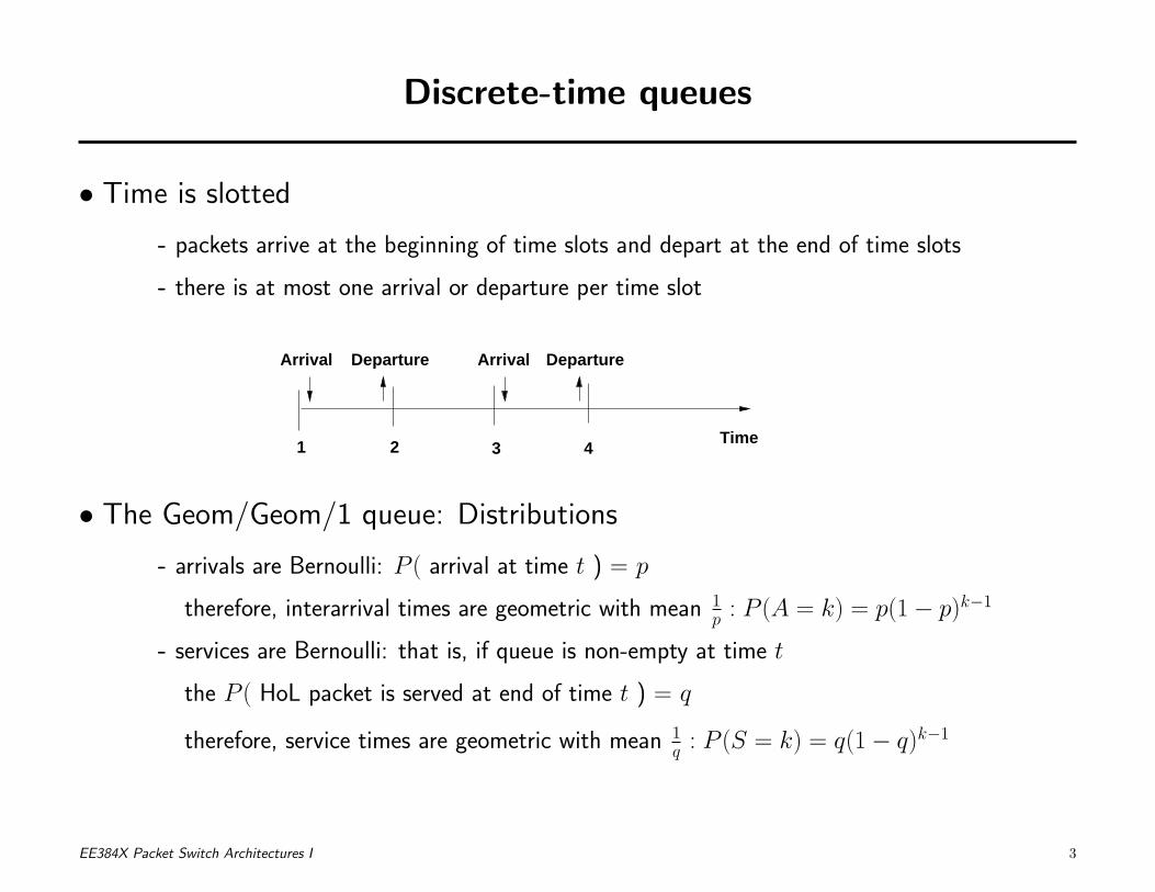
• Time is slotted

- packets arrive at the beginning of time slots and depart at the end of time slots

- there is at most one arrival or departure per time slot

2 3 41

Arrival Departure Arrival Departure

Time

• The Geom/Geom/1 queue: Distributions

- arrivals are Bernoulli: P ( arrival at time t ) = p

therefore, interarrival times are geometric with mean 1p : P (A = k) = p(1 − p)k−1

- services are Bernoulli: that is, if queue is non-empty at time t

the P ( HoL packet is served at end of time t ) = q

therefore, service times are geometric with mean 1q : P (S = k) = q(1 − q)k−1


The Geom/Geom/1 queue

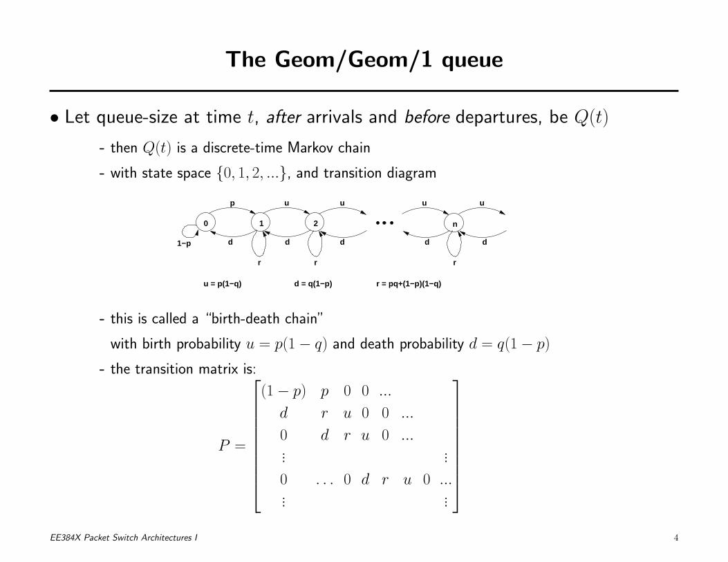
• Let queue-size at time t, after arrivals and before departures, be Q(t)

- then Q(t) is a discrete-time Markov chain

- with state space {0, 1, 2, ...}, and transition diagram

0 1 2

r r

p u u

d d d

n

r

u u

d d1−p

u = p(1−q) r = pq+(1−p)(1−q)d = q(1−p)

- this is called a “birth-death chain”

with birth probability u = p(1 − q) and death probability d = q(1 − p)

- the transition matrix is:

P =

(1 − p) p 0 0 ...

d r u 0 0 ...

0 d r u 0 ...... ...

0 . . . 0 d r u 0 ...... ...



• The equilibrium distribution π is obtained by solving π = πP

- π0 = (1 − p)π0 + dπ1 ⇒ π0 = dpπ1

- π1 = pπ0 + rπ1 + dπ2 ⇔ (d + u)π1 = uπ1 + dπ2 ⇔ uπ1 = dπ2

- for i ≥ 2, πi = uπi−1 + rπi + dπi+1 ⇔ uπi = dπi+1

• Therefore,

- πi =(

ud

)i−1π1, i ≥ 1, and π0 = q(1−p)

p π1

- since∑

i≥0 πi = 1, we get π1 = p(q−p)q2(1−p)

→ note that u < d is necessary, else∑

i≥0 πi = ∞

thus, for “stability” we need birth probability (u) < death probability (d)

• And

- letting ρ = ud , we get π1 = p(1−ρ)

q

- and P (Q = i) = π1ρi−1, i ≥ 1, P (Q = 0) = π1

q(1−p)p

- ρ is called the “load factor” and we have seen that ρ < 1 for stability

- this is equivalent to p < q (arrival rate < service rate)



• Some queueing quantities

- let Q be the steady-state number of packets in the queue, including the one in service

- then, E(Q) =∑

i≥1 iπi = π1

(1−ρ)2= p

q(1−ρ)

- let NQ be the steady-state number of packets in the queue, excluding the one in service

- then, NQ = Q − 1{Q>0} ⇒ E(NQ) = E(Q) − P (Q > 0) = pq(1−ρ) −

pq = pρ

q(1−ρ)


The M/M/1 Queue

• Specification

- arrivals occur according to a rate λ Poisson process

therefore, interarrival times are exp(λ): P (A > t) = e−λt

- service times are IID rate µ exponentials, and independent of arrivals

i.e. P (S > t) = e−µt

• Let Q(t) be the queue-size process at time t

- then Q(t) is a CTMC with state space {0, 1, 2, ...}

- so we need to find out the transition rates qij = γipij

• Determining γi: We know that γi = 1E(Ti)

, where Ti is the average time in

state i. There are two cases to consider

1. for i ≥ 1, Q(t) leaves i if there is an arrival or if there is a departure

E(Ti) = E(min{arrival time, service time}) =∫ ∞

0 P (min{A, S} > t) dt

=∫ ∞

0 P (A > t)P (S > t) dt =∫ ∞

0 e−(λ+µ)t dt = 1λ+µ

⇒ γi = 1E(Ti)

= λ + µ


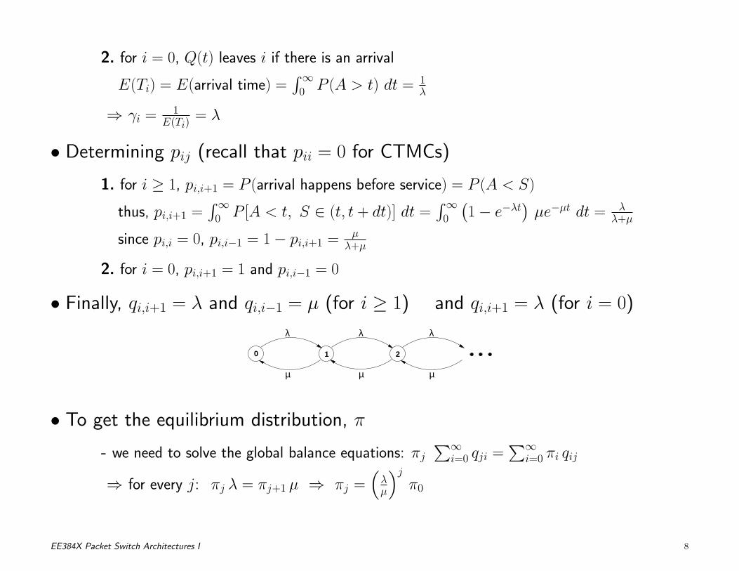
2. for i = 0, Q(t) leaves i if there is an arrival

E(Ti) = E(arrival time) =∫ ∞

0 P (A > t) dt = 1λ

⇒ γi = 1E(Ti)

= λ

• Determining pij (recall that pii = 0 for CTMCs)

1. for i ≥ 1, pi,i+1 = P (arrival happens before service) = P (A < S)

thus, pi,i+1 =∫ ∞

0 P [A < t, S ∈ (t, t + dt)] dt =∫ ∞

0

(

1 − e−λt)

µe−µt dt = λλ+µ

since pi,i = 0, pi,i−1 = 1 − pi,i+1 = µλ+µ

2. for i = 0, pi,i+1 = 1 and pi,i−1 = 0

• Finally, qi,i+1 = λ and qi,i−1 = µ (for i ≥ 1) and qi,i+1 = λ (for i = 0)

0 21

µ

λ λ λ

µµ

• To get the equilibrium distribution, π

- we need to solve the global balance equations: πj

∑∞i=0 qji =

∑∞i=0 πi qij

⇒ for every j: πj λ = πj+1 µ ⇒ πj =(

λµ

)j

π0


The M/M/1 Queue: Equilibrium or steady-state

• If

λ > µ: πj → ∞ and there is no steady-state

- this is to be expected, since more work is coming in than can be processed

- this is the unstable case

λ = µ: πj = π0 for every j

- since we require both 0 ≤ πj ≤ 1 and∑∞

j=0 πj = 1, there is again no equilibrium

- this is the critically unstable case

λ < µ: πj =(

λµ

)j

π0 is a geometrically decreasing sequence and∑∞

j=0 πj = 1 implies

- π0 = (1 − λµ); πj =

(

1 − λµ

) (

λµ

)j

- this is the stable case

• Quantities

- ρ = λµ is called the traffic intensity; if ρ < 1, then πj = (1 − ρ)ρj

- for ρ < 1, E(Q) =∑

j jπj = ρ1−ρ

- E(NQ) = E(Q − 1{Q>0}) = E(Q) − P (Q > 0) = ρ1−ρ − ρ = ρ2

1−ρ


Little’s Law

• This relates average queue-sizes and average waiting times

- holds quite generally - no distributional assumptions on arrivals and services

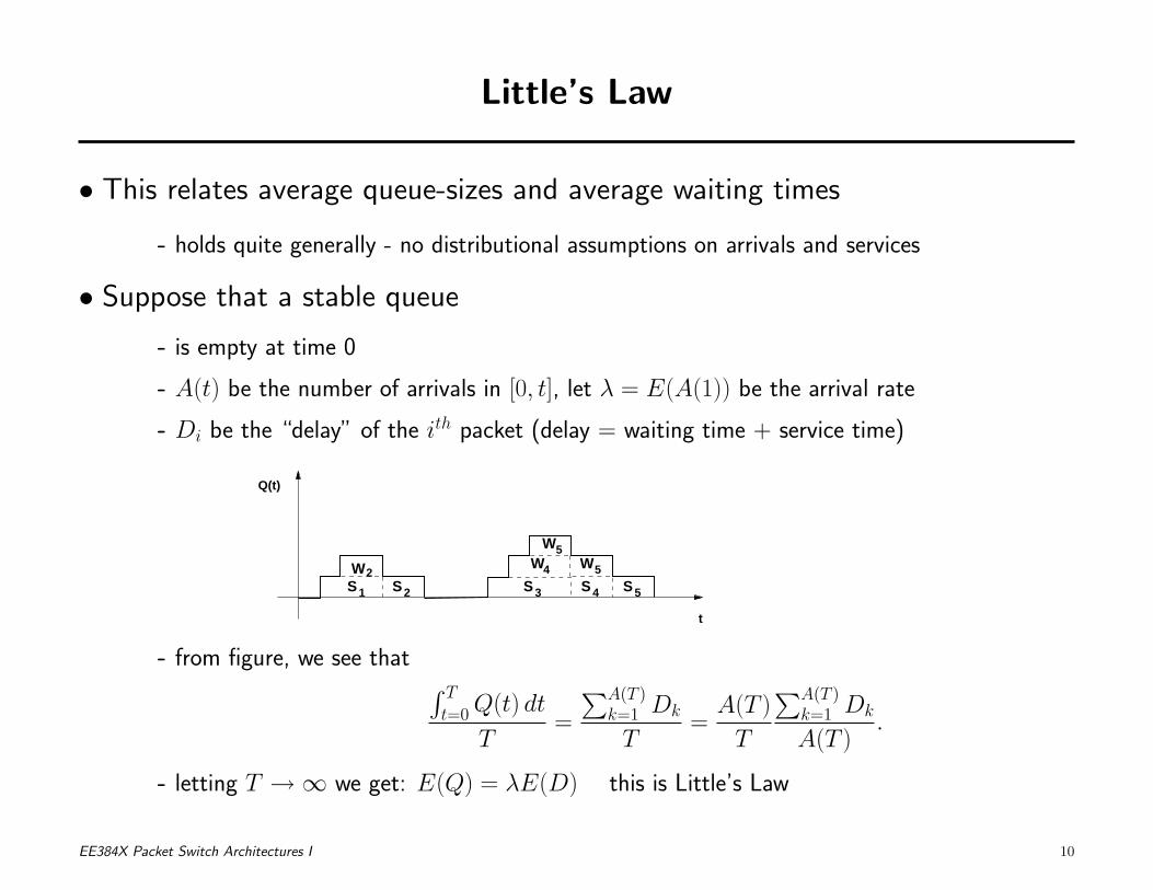
• Suppose that a stable queue

- is empty at time 0

- A(t) be the number of arrivals in [0, t], let λ = E(A(1)) be the arrival rate

- Di be the “delay” of the ith packet (delay = waiting time + service time)

W2

1S

W

3S 4S 5S

WW

4 5

5

S2

Q(t)

t

- from figure, we see that∫ T

t=0 Q(t) dt

T=

∑A(T )k=1 Dk

T=

A(T )

T

∑A(T )k=1 Dk

A(T ).

- letting T → ∞ we get: E(Q) = λE(D) this is Little’s Law


Some consequences

• For the Geom/Geom/1 queue

- we have seen that E(Q) = pq(1−ρ)

and arrival rate λ = p

- therefore, E(D) = E(Q)/λ = 1q(1−ρ)

- since waiting time = delay - service time,

- E(W ) = E(D) − E(S) = 1q(1−ρ) −

1q = ρ

q(1−ρ)

- by Little’s Law, E(NQ) = λE(W ) = p ρq(1−ρ)

• Similarly for the M/M/1 queue

- we have seen that E(Q) = ρ1−ρ

- therefore, E(D) = E(Q)/λ = 1µ(1−ρ) = 1

µ(µ−λ)

- since waiting time = delay - service time,

- E(W ) = E(D) − E(S) = λµ(µ−λ)

- again, by Little’s Law, E(NQ) = λE(W ) = λ2

µ(µ−λ) = ρ2

1−ρ


Other consequences: Back to delays and algorithms

• We have seen that bad scheduling algorithms can cause bad delay

- let’s understand this better

• Suppose we have

- N queues at which packets arrive (distribution of arrival process doesn’t matter)

- and there is a single server who serves

(1) from the longest queue (LQF)

(2) from the shortest queue (SQF)

- each packet takes one unit of time to serve (or transmit)

• Let

- (X l1(t), ..., X

lN(t)) be the queue sizes under LQF, and let S l(t) =

∑Ni=1 X l

i(t)

- (Xs1(t), ..., X

sN(t)) be queue sizes under SQF, let Ss(t) =

∑Ni=1 Xs

i (t)


• Under identical inputs we know that

- Sl(t) = Ss(t) for every t

- therefore, E(S l(t)) = E(Ss(t)) ⇒∑N

i=1 E(X li(t)) =

∑Ni=1 E(Xs

i (t))

- by symmetry (identical distribution of the arrivals to the N queues) we get

E(X li(t)) = E(X l

1(t)) and E(Xsi (t)) = E(Xs

1(t))

- therefore, E(S l(t)) = E(Ss(t)) ⇒ E(X li(t)) = E(Xs

1(t))

→ that is, the average occupancies under LQF and SQF are the same!

• To summarize

- throughputs under both LQF and SQF are the same

(because the server works just as often under both policies)

- furthermore, we have seen the average occupancies are the same

- by Little’s Law, this means the average delays are also the same

(because arrival rates are equal under both policies)

- what gives? i.e. does this mean the two policies are the same

so far as throughput and delay are concerned?


Let’s look at an example

• Take a 16 queue example

- arrivals at each queue are Bernoulli( 117) IID

- therefore, total load equals 16/17 = 0.9411

- the simulation results:

LQF: Average queue = 0.49959, average delay = 8.49206

SQF: Average queue = 0.498332, average delay = 8.47078

- sanity check: apply Little’s Law

1178.49206 = 0.49995 (Little miracles!)


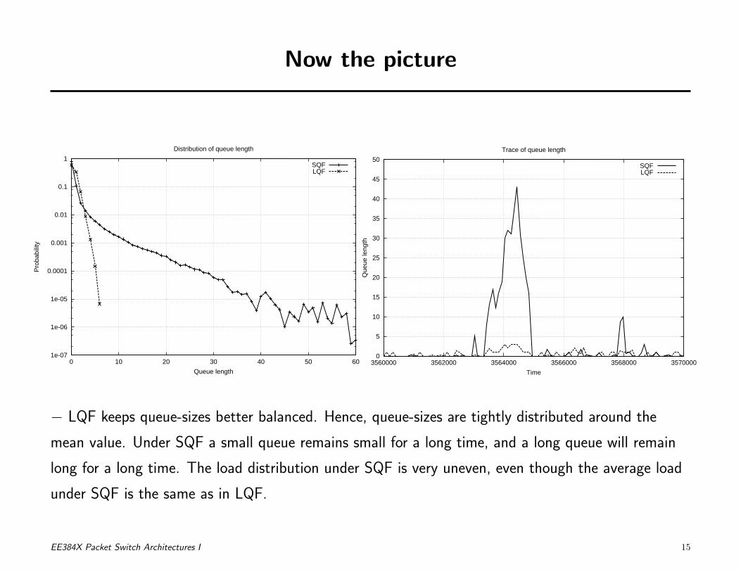
Now the picture

1e-07

1e-06

1e-05

0.0001

0.001

0.01

0.1

1

0 10 20 30 40 50 60

Pro

babi

lity

Queue length

Distribution of queue length

SQFLQF

0

5

10

15

20

25

30

35

40

45

50

3560000 3562000 3564000 3566000 3568000 3570000Q

ueue

leng

thTime

Trace of queue length

SQFLQF

− LQF keeps queue-sizes better balanced. Hence, queue-sizes are tightly distributed around the

mean value. Under SQF a small queue remains small for a long time, and a long queue will remain

long for a long time. The load distribution under SQF is very uneven, even though the average load

under SQF is the same as in LQF.


Poisson Arrivals See Time Averages (PASTA)

• Time and arrival averages. Consider a queue in equilibrium

- time average: πn = P (Q(t) = n), where t is an abitrary instance of time

- arrival average: an = P (arriving packet sees n packets in queue)

- Question: when is an = πn?

• Let’s begin with a “bad” example

- consider a queue where services are deterministic, equal to 3

- packets arrive at 1, 2, 3, 11, 12, 13, 21, 22, 23,. . .

- the evolution of the queue looks like ...

t

Q(t)

1 2 3 4 7 10


• Computing the probabilities

- π0 = 1/10, π1 = 4/10, π2 = 4/10 , π3 = 1/10

- a0 = 1/3, a1 = 1/3, a2 = 1/3

→ these are totally different!

- therefore, in general, time averages are not equal to arrival averages

• But

- if arrivals are Poisson (or Bernoulli, in discrete-time)

- then (we shall see that) time averages equal arrival averages

- this is PASTA - Poisson arrivals see time averages

• Implications

- to avoid falling victim to sampling bias, choose sampling instants completely randomly

- this makes sense (i.e. like random inspection)

- the beauty of the Poisson (or Bernoulli) process is that future arrivals

occur completely independently of past arrivals, and past arrivals are

what influence the present queue size!


PASTA, continued

• Consider a queue

- at which packets arrive as a Poisson process of rate λ

- the service distribution is arbitrary

- let πn be the prob that queue-size equals n at an arbitrary time t, say

- let an be the prob that an arrival sees a queue of size n

- then we get

an = P (Q(t) = n|A(t, t + δ) = 1)

(a)=

P (Q(t) = n, A(t, t + δ) = 1)

P (A(t, t + δ) = 1)

(b)=

P (Q(t) = n) P (A(t, t + dt) = 1)

P (A(t, t + dt) = 1)= P (Q(t) = n) = πn,

- where (a) is due to Bayes’ law

- and (b) uses the fact that arrivals after time t are independent of the queue-size at time t

→ therefore arrival averages equal time averages


The M/GI/1 Queue and the Pollaczek-Khinchine Formula

• Specification

- arrivals occur according to a rate λ Poisson process

therefore, interarrival times are exp(λ): P (A > t) = e−λt

- service times are IID and arbitrarily distributed with

i.e. mean E(S) = 1µ and second moment E(S2)

• Let the queue be in equilibrium and let

1. W (t) be the unifinished work in the system at time t

- i.e. W (t) is the amount of time from time t the server will be busy,

if no new work was allowed into the system after time t

- it is also the amount of time that a packet arriving at time t will have

to wait before being served

- W (t) is called the “work-load process” or the “waiting time process”

2. Si and Wi be the service and waiting times, respectively, of packet i.


W(t)

t

S

S

S

SS

1

2

3

4

5

{ {5W

W2 {W3

• Now

- notice that∫ T

0 W (t) dt

T=

∑A(T )k=1 Ak

T,

where Ak is the area of each of the triangles and the adjoining parallelogram

- thus∫ T

0 W (t) dt

T=

1

T

A(T )∑

k=1

(

S2k

2+ WkSk

)

=A(T )

T

1

A(T )

A(T )∑

k=1

(

S2k

2+ WkSk

)

- letting T → ∞, we get

E(Wtime) = λ

(

ES2

2+ E(W1S1)

)

= λ

(

ES2

2+ E(W1) E(S1)

)


- but since the arrivals are Poisson, by PASTA, E(Wtime) = E(W1)!

- therefore, letting E(Wtime) = E(W1) = E(W ), we get that

E(W ) =λ ES2

2(1 − λ E(S))=

λ ES2

2(1 − ρ)

- this is the famous Pollaczek-Khinchine formula

• Corollary: Determinism minimizes waiting

- consider an M/GI/1 queue

- allow the service time to be arbitrary, except that E(S) = 1µ

- since V ar(S) = ES2 − (ES)2 ≥ 0, we get that ES2 ≥ (ES)2 = 1µ2 .

- equality is achieved iff V ar(S) = 0; i.e. iff S is deterministic!

- this implies E(W ) = λES2

2(1−ρ) is smallest for deterministic services

(since the numerator is smallest in this case)

- or, determinism minimizes waiting


Stability

• Stability pertains to the question:

1. When does a system in which work arrives according to certain inputs

and in which work is removed in some fashion (i.e. service algorithms)

not allow work to become unbounded?

2. For example, if the system is describable as a Markov chain,

when is there an equilibrium such that the expected size is finite?

3. For us, it is equivalent to the question

when do switches or networks achieve 100% throughput?

• In the next few lectures

- we will understand what stability means

- find methods to establish the stability of algorithms

- know how to devise and use Lyapunov functions


An example

• Take 32 queues with dedicated servers

- service rate of each server = 1 packet/sec, service distributions are identical

- let packets arrive at rate λ

- packets are assigned upon arrival to:

(1) the shortest queue

(2) the longest queue

• What happens?

- under join the shortest queue

we get a maximum throughput of upto 32: λ can go upto (but less than) 32

- under join the longest queue

the maximum throughput is only 1: λ cannot increase beyond 1

→ the LQF policy completely underutilizes the capacity of the system

→ note: different stability regions under different schedules for same architecture


Stability

• In the previous example it was pretty obvious what was wrong with LQF

• In general, in switch scheduling algorithms

- it is far from obvious why a certain algorithm is not giving 100% throughput

- often, we know why an algorithm doesn’t do well by looking at counterexamples

- i.e. traffic patterns we construct that expose weaknesses in the algorithm

- likewise, we often know why an algorithm does well both based on intuition

and when we construct a proof to show that it gives 100% throughput

- the proofs usually involve the construction of Lyapunov (or potential) functions

→ we will learn more about counterexamples and about Lyapunov functions in

the next few lectures


Date post:	19-May-2020
Category:	Documents
Upload:	others
View:	12 times
Download:	0 times

Overview of Topics - Stanford University · Overview of Topics Intro to queueing theory...

Documents