DRAFT VERSION JANUARY 13, 2010 Preprint typeset using L A T E X style emulateapj v. 12/01/06 A CATALOG OF DETAILED VISUAL MORPHOLOGICAL CLASSIFICATIONS FOR 14034 GALAXIES IN THE SLOAN DIGITAL SKY SURVEY PREETHI BNAIR ∗ &ROBERTO GABRAHAM Department of Astronomy & Astrophysics, University of Toronto, 50 St. George Street, Toronto, ON, M5S 3H4. Draft version January 13, 2010 ABSTRACT We present a catalog of detailed visual classifications for 14034 galaxies in the Sloan Digital Sky Survey (SDSS) Data Release 4 (DR4). Our sample includes nearly all spectroscopically-targeted galaxies in the red- shift range 0.01 <z< 0.1 down to an apparent extinction-corrected limit of g< 16 mag. In addition to T-Types we record the existence of bars, rings, lenses, tails, warps, dust lanes, arm flocculence and multiplicity. This sample defines a comprehensive local galaxy sample which we will use in future papers to study low redshift morphology. It will also prove useful for calibrating automated galaxy classification algorithms. In this paper we describe the classification methodology used, detail the systematics and biases of our sample and summarize the overall statistical properties of the sample, noting the most obvious trends that are relevant for general comparisons of our catalog with previously published work. Subject headings: galaxies: fundamental parameters, galaxies: photometry, galaxies: morphology 1. INTRODUCTION Considerable progress has been made in developing tech- niques for automated classification of galaxies. However, the disappointing fact is that, at present, state-of-the-art auto- mated galaxy classification is only capable of delivering crude classifications, albeit very quickly. The large numbers of classifications delivered by automated techniques have proved highly useful in their appropriate context, but they are neither as accurate, nor as comprehensive, as visual classifications made by a trained observer. The strengths and limitations of present machine-based galaxy classification techniques should not come as a surprise if one reflects upon the fact that something like half the human brain is devoted to vision. Millions of years of evolution have refined our brain’s capacity for image processing and analy- sis to the extent that a well-trained human can classify an in- dividual image more accurately than a computer-based algo- rithm in essentially every field of science or industry in which comparisons have been made. For example, even state-of- the-art automated facial recognition systems cannot presently identify a human face with the accuracy routinely delivered by cursory visual inspection. Nevertheless, the basic simplic- ity of galaxies’ structural forms suggests there is considerable room for improving automated classifications using more so- phisticated tools for pattern recognition. An important step toward this goal is the development of a robust training set of digital galaxy images with detailed visual classifications. Such a training set would also prove useful for many programs of investigation which probe the systematics of galactic struc- ture. Inspired by the evident need for a catalog of detailed visual morphological classifications of local galaxies, we have un- dertaken to classify a g-band apparent magnitude limited sam- ple of 14034 galaxies from Sloan Digital Sky Survey (SDSS) Data Release 4. Our catalog is six times larger than the catalog of visual classifications presented in Fukugita et al. (2007). However our goal is to not just increase the size ∗ Present address: INAF - Astronomical Observatory of Bologna, Via Ran- zani 1, 40127 Bologna, ITALY Electronic address: [email protected],[email protected]of our sample relative to previous work, but also to take vi- sual classifications in the SDSS to a more detailed level rem- iniscent of earlier generations of catalogs (e.g. the Hubble Atlas (Sandage 1961), the Revised Shapley-Ames Catalog (Sandage & Tammann 1981), and the de Vaucouleurs Atlas (de Vaucouleurs 1963; de Vaucouleurs et al. 1991)). In addi- tion to T-Types, our catalog attempts to record subtle morpho- logical features such as the existence and prominence of bars, rings, lenses, tails, shells, warps and dust lanes, and the nature of spiral structure (arm flocculence and multiplicity). Our catalog is presented with two main goals in mind: 1. We seek to provide a generally useful comprehensive local sample with highly detailed morphological classi- fications. Future papers in this series will use this cat- alog to explore the local abundance and evolutionary properties of rings, bars, ansae, spiral structure, dust and tidal features in galaxies. 2. The catalog is a starting point for future attempts to im- prove automated galaxy classification by incorporating detection algorithms for subtle morphological features. With the exception of some simple attempts to auto- mate the detection of galactic bars, to date no automated classification method attempts to characterize the ‘fine structure’ of galaxy morphology. A plan for this paper follows. In Section 2 we describe our sample, and note its strengths and limitations. Section 3 describes our classification methodology and Section 4 presents a number of image montages which illustrate our classification scheme. Section 5 compares our classifications against those from other studies in order to estimate the reliability of our catalog. Systematic effects introduced by seeing, inclination and distance are explored in Section 6. The catalog itself is presented in Section 7, which is the heart of this paper. Summary statistics for our sample as a whole are presented in Section 8. We conclude in Section 9. Throughout this paper we assume a flat Λ-dominated cosmology with h =0.7, Ω M =0.3 and Ω Λ =0.7.
Transcript
DRAFT VERSIONJANUARY 13, 2010Preprint typeset using LATEX style emulateapj v. 12/01/06
A CATALOG OF DETAILED VISUAL MORPHOLOGICAL CLASSIFICATIONS FOR 14034 GALAXIES IN THE SLOANDIGITAL SKY SURVEY
PREETHI B NAIR∗ & ROBERTOG ABRAHAMDepartment of Astronomy & Astrophysics, University of Toronto, 50 St. George Street, Toronto, ON, M5S 3H4.
Draft version January 13, 2010
ABSTRACTWe present a catalog of detailed visual classifications for 14034 galaxies in the Sloan Digital Sky Survey
(SDSS) Data Release 4 (DR4). Our sample includes nearly all spectroscopically-targeted galaxies in the red-shift range0.01 < z < 0.1 down to an apparent extinction-corrected limit ofg < 16 mag. In addition toT-Types we record the existence of bars, rings, lenses, tails, warps, dust lanes, arm flocculence and multiplicity.This sample defines a comprehensive local galaxy sample which we will use in future papers to study lowredshift morphology. It will also prove useful for calibrating automated galaxy classification algorithms. Inthis paper we describe the classification methodology used,detail the systematics and biases of our sample andsummarize the overall statistical properties of the sample, noting the most obvious trends that are relevant forgeneral comparisons of our catalog with previously published work.Subject headings:galaxies: fundamental parameters, galaxies: photometry,galaxies: morphology
1. INTRODUCTION
Considerable progress has been made in developing tech-niques for automated classification of galaxies. However,the disappointing fact is that, at present, state-of-the-art auto-mated galaxy classification is only capable of delivering crudeclassifications, albeit very quickly. The large numbers ofclassifications delivered by automated techniques have provedhighly useful in their appropriate context, but they are neitheras accurate, nor as comprehensive, as visual classificationsmade by a trained observer.
The strengths and limitations of present machine-basedgalaxy classification techniques should not come as a surpriseif one reflects upon the fact that something like half the humanbrain is devoted to vision. Millions of years of evolution haverefined our brain’s capacity for image processing and analy-sis to the extent that a well-trained human can classify an in-dividual image more accurately than a computer-based algo-rithm in essentially every field of science or industry in whichcomparisons have been made. For example, even state-of-the-art automated facial recognition systems cannot presentlyidentify a human face with the accuracy routinely deliveredby cursory visual inspection. Nevertheless, the basic simplic-ity of galaxies’ structural forms suggests there is considerableroom for improving automated classifications using more so-phisticated tools for pattern recognition. An important steptoward this goal is the development of a robust training setof digital galaxy images with detailed visual classifications.Such a training set would also prove useful for many programsof investigation which probe the systematics of galactic struc-ture.
Inspired by the evident need for a catalog of detailed visualmorphological classifications of local galaxies, we have un-dertaken to classify ag-band apparent magnitude limited sam-ple of 14034 galaxies from Sloan Digital Sky Survey (SDSS)Data Release 4. Our catalog is six times larger than thecatalog of visual classifications presented in Fukugita et al.(2007). However our goal is to not just increase the size
∗Present address: INAF - Astronomical Observatory of Bologna, Via Ran-zani 1, 40127 Bologna, ITALYElectronic address: [email protected],[email protected]
of our sample relative to previous work, but also to take vi-sual classifications in the SDSS to a more detailed level rem-iniscent of earlier generations of catalogs (e.g. the HubbleAtlas (Sandage 1961), the Revised Shapley-Ames Catalog(Sandage & Tammann 1981), and the de Vaucouleurs Atlas(de Vaucouleurs 1963; de Vaucouleurs et al. 1991)). In addi-tion to T-Types, our catalog attempts to record subtle morpho-logical features such as the existence and prominence of bars,rings, lenses, tails, shells, warps and dust lanes, and the natureof spiral structure (arm flocculence and multiplicity).
Our catalog is presented with two main goals in mind:
1. We seek to provide a generally useful comprehensivelocal sample with highly detailed morphological classi-fications. Future papers in this series will use this cat-alog to explore the local abundance and evolutionaryproperties of rings, bars, ansae, spiral structure, dustand tidal features in galaxies.
2. The catalog is a starting point for future attempts to im-prove automated galaxy classification by incorporatingdetection algorithms for subtle morphological features.With the exception of some simple attempts to auto-mate the detection of galactic bars, to date no automatedclassification method attempts to characterize the ‘finestructure’ of galaxy morphology.
A plan for this paper follows. In Section 2 we describeour sample, and note its strengths and limitations. Section3 describes our classification methodology and Section 4presents a number of image montages which illustrate ourclassification scheme. Section 5 compares our classificationsagainst those from other studies in order to estimate thereliability of our catalog. Systematic effects introducedbyseeing, inclination and distance are explored in Section 6.The catalog itself is presented in Section 7, which is theheart of this paper. Summary statistics for our sample as awhole are presented in Section 8. We conclude in Section9. Throughout this paper we assume a flatΛ-dominatedcosmology withh = 0.7, ΩM = 0.3 andΩΛ = 0.7.
FIG. 1.— [Left] Absolute magnitude vs. redshift for our sample of 14034 SDSS galaxies withg < 16 mag. The horizontal line corresponds to the characteristicmagnitudeM⋆ of the SDSS luminosity function determined by Blanton et al.(2003). Vertical lines are the redshift cuts atz = 0.05 andz = 0.1 describedin the text. The light grey points show the distribution of the entire Data Release 4 main galaxy sample up toz < 0.3. The intermediate grey points show thedistribution of the sample withz < 0.05 while the dark grey points show the distribution with0.05 < z < 0.1. [Right] Logarithm of the stellar mass (fromKauffmann et al. (2003b)) as a function of redshift. As expected from the left-hand panel, we see the brightest and most massive galaxies dominate our sampleat z>0.05.
FIG. 2.— Number of galaxies vs. absolute g-band magnitude for our sample of 14034 SDSS galaxies with 0.01<z<0.1 andg < 16 mag (extinction corrected).The light grey area shows the distribution of the sample withz < 0.05 while the dark grey area shows the distribution with0.05 < z < 0.1. Note that the bulkof the bright galaxy population is missed with az < 0.05 cut. See text for details on sample selection.
2. SAMPLE
2.1. Sample Selection
The local sample presented here is derived fromthe SDSS (Stoughton et al. 2002; York et al. 2000;Adelman-McCarthy et al. 2006) DR4 release which covers6670 sq. deg in theu’,g’,r’,i’,z’ filters. (The central wave-lengths of these filters are 3553A, 4686A, 6166A, 7480A,and 8932A, respectively). The galaxies are selected from thespectroscopic main sample described in Strauss et al. (2002).We use the DR4 photometry catalogs to select all objectswith an extinction correctedg’ band magnitude brighter than16 mag at redshiftsz less thanz = 0.1, which gives usa sample of 14700 galaxies. Objects mistakenly classifiedas galaxies have been removed. The current catalog alsoexcludes all objects at redshifts belowz ∼ 0.01, becauseextraction of extended galaxies for quantitative analysisatsuch low redshifts is difficult on the basis of SDSS Atlaspipeline images which leaves us with a sample of 14034galaxies.
The upper redshift limit ofz = 0.1 in our sample is chosenin order to exclude objects where morphological detail is diffi-cult to detect because of distance effects. As will be discussednext, to some extent the choice of this upper redshift limit isa balance between seeking to include a fair sample of mas-sive galaxies while at the same time recognizing the inherentlimitations on the classification of faint galaxies imposedby
variable seeing and relatively low signal-to-noise in the SDSSimaging data.
Figure 1 shows the absolute magnitude and stellar massdistribution of galaxies (see§2.2 for a discussion of thesemass estimates) as a function of redshift for SDSS DR4(light gray) along with our sub-sample of DR4 galaxies (darkgray). The public-domainK-Correct software (version 4;Blanton et al. (2005)) was used to derive the K-correctionsneeded to produce this figure. At a redshift ofz ∼ 0.05the SDSS images probe a physical resolution similar to thatprobed by theHubble Space Telescope(HST) viewing galax-ies atz ∼ 1. We hope our classifications will be useful as acomplement to HST evolutionary studies out to at leastz ∼ 1,so in some sensez ∼ 0.05 (instead ofz ∼ 0.1 as we have cho-sen) would have been a sensible upper limit for our classifi-cations, because beyond this redshift the rest-frame resolutionof the SDSS data is actually poorer than that of HST probingz = 1 galaxies1 However, Figure 1 shows that making a cutat z = 0.05 would have resulted in our missing most of thebright, massive galaxy population (systems brighter thanM∗,the characteristic magnitude of the luminosity function).Thisis further emphasized by Figure 2 which shows the distribu-tion of absolute magnitudes in our sample forz ≤ 0.05 (lightgray) andz ≤ 0.1 (dark gray). Belowz = 0.05 we do not
1 The HST Advanced Camera for Survey’s image scale of 0.04′′/pixel cor-responds to a physical scale of 0.32 kpc/pixel atz = 1. The SDSS telescope’s0.4′′/pixel corresponds to 0.74 kpc/pixel at z∼0.1.
3
probe enough cosmic volume to include manyM∗ galaxies inthe sample, but such bright objects are the focus of many high-redshift studies. We therefore decided to increase our redshiftlimit to z = 0.1 at the expense losing some resolution in therest-frame.
The catalog presented in this paper is statistically more rep-resentative for detailed morphological studies than any othersample published to date. For example, there are essentiallyno galaxies fainter thanMg ∼ −19 mag in the analyses pre-sented by Frei et al. (1996) and van den Bergh et al. (2002).Recent morphological catalogs by Fukugita et al. (2007) andDriver et al. (2006) do not provide the visual detail presentedhere. However, it need hardly be emphasized that because ofthe redshift and magnitude cuts just described, our sample isby no means volume-limited, and something like theVmax
formalism should be incorporated when using the catalog inthis paper to calculate space densities. Evolutionary changesin morphology are perceptible atz ∼ 0.5 (e.g.a change in thefraction of massive galaxies with bars; Abraham et al. 1999,Sheth et al. 2008), but we expect such changes to be imper-ceptible for objects atz < 0.1, and therefore treat the entiresample as ‘local’.
2.2. Supplementary data
For the convenience of the reader, we have augmented ourcatalog of morphological classifications with published sup-plementary data derived by other groups. Sersic profile pa-rameters and environmental density estimates from the NYUgroup (Blanton et al. 2003) have been included. Environmentestimates from Baldry et al. (2006) and the Yang et al. (2007)SDSS group catalog have also been included. We also includederived stellar masses, ages, and star formation rates fromtheGarching group (Kauffmann et al. 2003b,c; Brinchmann et al.2004). The reader is referred to the original papers cited abovefor details on how these parameters were derived.
3. CLASSIFICATION METHODOLOGY
The galaxy classification scheme used here is primarilybased on the Carnegie Atlas of Galaxies (Sandage & Bedke1994) in consultation with the Third Reference Catalog ofBright Galaxies (de Vaucouleurs 1963), RC3, along with im-ages for many fiducial objects obtained using the IPAC NEDdatabase. Traditional methods for classification involve print-ing galaxy images at various contrast ratios and manually in-putting the classification back into a table. For the∼ 14000objects in our sample this would be very cumbersome. Wetherefore developed web-based graphical display softwaretoallow us to inspect images at multiple contrast levels andrecord our classifications directly into a database.
After experimenting with a large subsample of objects inall 5 bands to determine in a general way the most effi-cient path forward, we adopted the following classificationprocedure. The registered SDSS fpC reduced frames wasused to re-extract the galaxies in all bands with SExtractor(Bertin & Arnouts 1996), using ther′-band image as the tem-plate. The segmentation of each galaxy was checked visu-ally to ensure ‘parent’ and ‘child’ objects were correctly sepa-rated. Small ‘postage stamp’ images (of width 50h−1 kpc and100h−1 kpc) were then created for each object in each band at5 contrast ratios determined by the flux range spanned by thegalaxy. For any object where the automatically-chosen con-trast ratios were not appropriate for identification purposes,we used ds9 manually to inspect images at a range of con-trast ratios. The T-Types for the entire sample was classified
twice by the first author, with a mean deviation of less than0.5 T-Types.
While we found that a clear distinction between the vari-ous Hubble subclasses was possible to make for most of ourobjects, not all classifications are clear-cut. Therefore someclassifications are suffixed by flags using a notation whichindicates that the classification is somewhat doubtful (?),orthat the galaxy is peculiar (p), or simply that the classifica-tion is highly uncertain (:). This notation is adopted from theRC3 scheme. It should be noted that a (p) implies a pecu-liarity in a galaxy such as the presence of shells or tidal tailsor some other feature (for which the secondary flags needto be checked) and not a ‘Peculiar’ galaxy. Peculiar galax-ies, or galaxies which could not be classified as a standardHubble type have been assigned a T-Type of ‘99’ (unknown).Secondary characteristic flags may be set for both normalT-Types and unknown galaxies, such as the ‘bulge-like’, or‘disk-like‘ flags or one of the Elmegreen et al. (2005) types(‘clump-clusters’, ‘tadpoles’, ‘doubles’, and ‘chains’)whichhave entered into the lexicon of high-redshift galaxy forms.It should be noted that our purpose in adding the latter sec-ondary flags to our catalog is not only to identify probable lo-cal counterparts to these high redshift types, but also to iden-tify objects which might be confused with such objects if seenat higher redshifts. For example, we flagged a number of ob-jects that would seem to us to be rapidly star-forming clumpyspirals that would resemble clump clusters if seen further tothe UV and with slightly poorer resolution. Since we havebeen fairly liberal in assigning Elmegreen et al. (2005) types,due care should be taken when analyzing these subsamples,and we feel this categorization in our catalog is mainly usefulfor identifying samples worthy of follow-up observations.
As has already been emphasized, a major goal of our cat-alog is to capture information on a range of morphologicalproperties beyond a galaxy’s basic type. Henceforth we willrefer to properties such as bars, rings, lenses, ansae, tidal tailsand the details of spiral structure as a galaxy’sfine structure.We noted the existence of a broad range of fine structure.Stellar bars were classified as the following types: strong,intermediate, weak, ansae and peanut. Rings were classi-fied as nuclear, inner, outer, pseudo-outer (R1/R2), and col-lisional. Lenses were classified as inner or outer. Arm typesfrom grand design to flocculent were recorded, as well as armlength and multiplicity. We recorded the presence of dustlanes, galaxy orientation, interaction features such as tails,warps, shells and bridges, the morphology of the nearest in-teracting galaxy and the merger orientation. Classificationswere done using theg′-band images, though to confirm thepresence of some features, like bars, we opted to check ther′
andi′ band data as well. T-Types are based solely on theg′-band images. We ultimately decided to exclude informationdetermined from theu′-band andz′-band images completelydue to poor signal-to-noise ratios.
4. ILLUSTRATIONS OF REPRESENTATIVE GALAXIES
In this section we present color montages constructed byassigning RGB colors tog′, r′, i′ data channels. These colorimages were taken from the SDSS Imaging Server. In or-der to allow the reader to compare our classifications to thosefrom other sources, we have tried to choose objects in thesemontages that are part of the small sample of objects in ourcatalog that overlap with other published samples (e.g. theRC3, or the catalog of Fukugita et al. 2007). Aside from thisconstraint, the galaxies in these montages have been selected
4
at random from the catalog.
4.1. Galaxies with Classical Forms (Standard T-Types)
Figures 3 and 4 show color composite images of a numberof E through Sd galaxies in our catalog which have RC3 orFukugita et al. (2007) classifications. In§5 we will present adetailed comparison of our classifications against those givenin earlier work, but at this stage it is perhaps worthwhile toforeshadow this discussion by referring the reader to Table1,which shows the relation between RC3 T-Types, our T-Types,and those of Fukugita et al (2007)2. For illustrative purposesin these figures we have grouped sub-categories of galaxiesinto broader classes: E and E/S0 galaxies are shown together,as are S0 and S0/a galaxies, Sa and Sab galaxies, Sb and Sbcgalaxies, Sc and Scd galaxies and galaxies with T-Types laterthan Sd. The J2000 object identifier is listed at the top of eachgalaxy’s panel, along with our own T-Type (PN T-Type) andthe RC3 type3 or Fukugita et al. (2007) T-Type. The objectsare arranged in order of decreasing stellar mass. We remindthe reader that the presence or absence of a dust lane is notused as a classification criterion.
4.2. Galaxies with Unusual Forms
There are 353 objects which do not have a regular T-Typeclassifications in this catalog. These objects have had T-Typesof ‘99’ assigned to them, and the great majority of these ob-jects represent objects that do not find a natural home in theHubble Sequence, although a few are simply galaxies that wefelt were too small to reliably classify. Wherever possiblegalaxies with unusual forms have been assigned flags in ourcatalog which correspond to secondary classifications, suchas ‘bulge-like’ or ‘disk-like’ and in some cases the high red-shift sub-classifications of ‘clump cluster’, ‘double’, ‘tadpole’and ‘chain’ introduced by Elmegreen et al. (2005). Galaxieswhere a sub-class could not be assigned are more likely to bemergers and the appropriate merger flags have been set.
Figure 5 shows a montage of galaxies with unusual forms.Since this category of objects is rather broad, the reader willprobably wish to subdivide it to isolate interesting objects us-ing the secondary indicators noted earlier. For example, thereader can easily filter the catalog for objects that are unusualbecause they are somewhat too small to be reliably classi-fied (top two rows), or objects that are unusual with struc-ture suggestive of being at an early stage of merging (mostobjects in the middle two rows), and objects that appear tobe near the end stages of a merger (most objects in the bot-tom two rows). The reader should note that while secondaryflags in the catalog can be used to assign most objects intothese three bins (‘too small to classify’, ‘early-phase merger’,and ‘late-phase merger’), many interesting objects cannotbeclassified as any of these. For example, the last object in thelast row, J155308.66+540850.42, appears to be a double col-lisional ring system, which we have been calling ‘Preethi’sCross-Eyed Galaxy’. The rarity of collisional rings makes it
2 We also remind the reader that an easy way to remember the numericequivalent for a T-Type is to note that all major classes are odd numbers (e.g.Sa galaxies have T-Type 1, and Sb galaxies have T-Type 3), while the finerseparation are even numbers (e.g. Sab has T-Type 2).
3 The RC3 short form classification is made up of 7 characters which start-ing from the left identify (1) peculiarities such as outer rings: ’R’ for full, ’P’for pseudo, (2) Crude class: E for elliptical, L for lenticular or S for spiral (3)bar class: B for strong bar, X for weak bar, A for no bar, (4) inner rings, Ror lenses, L, (5) T-Type for example 3 for Sb, (6) flags like unsure(?) and (7)flags.
unlikely that this system is an optical superposition of twocollisional rings, but on the other hand numerical simulationsof ‘bullseye’ collisions do not (at present) generate multiplerings.
Figure 6 shows galaxies which we have sub-classified as be-ing (possible) low-redshift equivalents of high-z clump clus-ters (top panel), doubles (middle panel) or tadpole galaxies(bottom panel) as defined by Elmegreen et al. (2005). As hasalready been noted, in some cases (for example the clumpcluster J074156.00+411339.50 in the top panel, second row,third column) these objects appear to be bona-fide counter-parts to high-redshift galaxy forms, while in other cases weshow objects which could easily be mistaken for these formsat high redshifts (e.g. J232123.51-093134.93, which is a veryclumpy asymmetric spiral galaxy). Note that we found no ex-amples of chain galaxies at z>0.01.
4.3. Fine Structures
Figures 7 – 12 show representative examples of the finestructures we have classified in our objects. Once again, weshow systems with the J2000 object identifier listed at the top,the galaxy redshift at the bottom left and our T-Type classifi-cation at the bottom right. A comparison of the fine structuresrecorded in these figures with those captured by the RC3 clas-sifications for these objects will be shown in§5.
4.3.1. Bars
Figure 7 shows a random sample of galaxies with strong,intermediate and weak bars. The strength of the bar is definedin terms of the size of the bar compared to the galaxy diame-ter and its prominence. In our system, we refer to those barsthat dominate that light distribution as strong bars. Weak barsare smaller in size and contain only a small fraction of thetotal flux of the galaxy. Intermediate bars span the range be-tween strong and weak bars.It is important to note that in ourscheme all the bar types are viewed as definite bars — this isunlike the RC3 scheme, where systems classed weakly barredinclude objects that possibly contain bars.In this sense oursystem is more conservative than that of the RC3, and (as willbe shown in the next section) our bar fraction is lower. Itis also worth noting that our classification of bar strength isbased on inspection of theg′-band images but the determina-tion of a bar’s existence was based on studying each galaxyin all three bands (g′, r′, i′). However, in nearly every case(98% of the time) bars observed in ther′ andi′ bands are alsoobserved ing′. As expected, many of our barred objects havea ring or lens component. We will investigate the connectionbetween rings and bars in a later paper in this series.
4.3.2. Rings and Lenses
Figure 8 shows a montage of inner (top panel), outer (mid-dle panel) and combination (bottom panel) ringed galaxies,and Figure 9 shows a montage of galaxies with inner lenses(top panel) or outer lenses (bottom panel). Inner rings aremore easily identified when bars are present. In galaxies with-out bars, inner ring classifications are much harder due to con-fusion with outer rings. Outer rings and pseudo outer rings asdefined by Buta & Combes (1996) are also distinguishable.Confusion can occur with lens galaxies as in Figure 9 and col-lisional ring systems. Lens galaxies (or galaxies with regionsof constant surface brightness) can exhibit either an inneroran outer lens. Both lens types can lead to the correspond-ing rings. There may be systems where outer rings eventuallyform lenses (Buta & Combes 1996).
5
FIG. 3.— A montage of images representingTop: E + E/S0 galaxies,Middle: S0+ S0a galaxies, andBottom: Sa + Sab galaxies (2 rows for each) as classifiedby the first author (PN). In each of these categories, galaxies are arranged in order of decreasing stellar mass. The J2000object identifier is listed at the top withthe redshift and the RC3 classification at the bottom. The seven possible letters starting from the left in the RC3 designation identify (1) peculiarities such asouter rings ’R’, (2) Type: E for elliptical, L for lenticularor S for spiral (3) bar class: B for strong bar, X for weak bar, Afor no bar, (4) inner rings, (5) T-Typeeg 3 for Sb. Fields (6) and (7) are used for additional flags, like unsure (?). Each stamp is 50h−1 kpc on a side.
6
FIG. 4.— A montage of images representing Sb, Sc and Sd galaxies (2 rows for each) as classified by the first author (PN). In each of these categories, galaxiesare arranged in order of decreasing stellar mass. The J2000 object identifier is listed at the top with the redshift and theRC3 classification at the bottom (whenavailable). The seven possible letters starting from the left in the RC3 designation identify (1) peculiarities such asouter rings ’R’, (2) Type: E for elliptical, Lfor lenticular or S for spiral (3) bar class: B for strong bar,X for weak bar, A for no bar, (4) inner rings, (5) T-Type eg 3 forSb (6 and 7) flags like unsure(?).Each stamp is 50h−1 kpc on a side. Although color images are shown, the classification was carried out on the g-band images. See text for details.
7
FIG. 5.— A montage of images representing unknown (T-Type=99) galaxies.Top: Examples of objects deemed too small for reliable classification. These aredwarf galaxies, perhaps dwarf spheroidals or dwarf spirals. Middle: Objects grossly distorted by merging/interactions.Bottom: Likely end stages or remnantsof mergers. Objects are arranged in order of increasing mass. The J2000 object identifier is listed at the top with the redshift and the author classification at thebottom. Each stamp is 50h−1 kpc on a side. Although color images are shown, the classification was carried out on the g-band images. See text for details. Thecolor images are taken from the SDSS Imaging Server.
8
FIG. 6.— A montage of images representing galaxies which may be classified as (or easily mistaken for, at higher redshift) theElmegreen et al. (2005)designations of[Top] Clump Cluster (CC),[Middle] Double galaxies (DB) and[Bottom] Tadpole galaxies (Td). As described in the text, in a few cases thesesecondary classifications have been assigned to objects mainly because we felt that, if seen at higher redshift and in therest-frame UV, these galaxies wouldresemble systems such as clump clusters. The J2000 object identifier is listed at the top with the redshift and the author classification at the bottom. Each stampis 50h−1 kpc on a side. Although color images are shown, the classification was carried out on the g-band images. See text for further details. The color imagesare taken from the SDSS Imaging Server.
9
FIG. 7.— A montage of images representingTop: Strong bars,Middle: Medium bars andBottom: Weak bars (2 rows for each) as classified by the authorarranged in order of T-Type. Strong bars are comparable in size to the galaxy and have a significant amount of the total flux of the galaxy. Weak bars are smallerin size and contain a small fraction of the total flux of the galaxy. Intermediate bars span the range between strong and weak bars. The J2000 object identifier islisted at the top with the redshift and the author classification at the bottom. Each stamp is 50h−1 kpc on a side. Our classification of bar strength is based oninspection of theg′-band images but the determination of a bar’s existence was based on studying each galaxy in all three bands (g′, r′, i′). Color images werenot used to determine the ‘strength’ of the bar. See text for details. The color images are taken from the SDSS Imaging Server.
10
FIG. 8.— A montage of images representing inner rings, outer rings and objects with both (2 rows for each) as classified by the author. Inner rings are moreeasily identified in barred object where they begin near where the bars end. Partial rings have also been included in this category. Outer rings are fairly easilyidentified in most systems. Pseudo-Rings as defined by Buta (1990) are included in this category. Confusion can arise in systems with no bars and only one ringas well as with collisional ring systems. The J2000 object identifier is listed at the top with the redshift and the author classification at the bottom. Each stamp is50h−1 kpc on a side. Although color images are shown, the classification was carried out on the g-band images. See text for details. The color images are takenfrom the SDSS Imaging Server.
11
FIG. 9.— A montage of images representing Inner and Outer lenses(3 rows for each) as classified by the author. The lenses are seen as regions of near constantsurface brightness with very little variation with radius.Inner lenses are most easily identified when they have an outer ring. Outer lenses can also lead to outerrings. The J2000 object identifier is listed at the top with the redshift at the bottom left and the author classification atthe bottom right. Each stamp is 50h−1
kpc on a side. Although color images are shown, the classification was carried out on the g-band images. See text for details. The color images are taken fromthe SDSS Imaging Server.
12
FIG. 10.— A montage of images representing short, medium and long tidal tails (2 rows for each) as classified by the author. Tidal tails are classified into thethree categories based on comparison with the host galaxy size. If the tails are much larger than the galaxy, they are classified as long tails. Tails comparable insize to the galaxy are classified as medium tails while those much smaller than the galaxy are classified as short tails. Many objects display multiple tails. TheJ2000 object identifier is listed at the top with the redshiftat the bottom left and the author classification at the bottomright. Each stamp is 50h−1 kpc on aside. Although color images are shown, the classification was carried out on the g-band images. See text for details. The color images are taken from the SDSSImaging Server.
13
FIG. 11.— A mosaic of images representing collisional ring systems, which are ringed galaxies formed by bulls-eye collision between two galaxies, as classifiedby the author. The classification into collisional rings is based on the color stamp of the galaxy (as the rings are normally blue), the shape of the ring and on thepresence of spokes. The J2000 object identifier is listed at the top with the redshift and the author classification at the bottom. Each stamp is 50h−1 kpc on aside. The color images are taken from the SDSS Imaging Server.
FIG. 12.— A mosaic of images representing shells as classified bythe author. The J2000 object identifier is listed at the top with the redshift and the authorclassification at the bottom. Each stamp is 50h−1 kpc on a side. Although color images are shown, the classification was carried out on the g-band images. Seetext for details. The color images are taken from the SDSS Imaging Server.
14
FIG. 13.— A mosaic of images representing paired systems. The J2000 object identifier is listed at the top with the redshift and the author classification atthe bottom. Each stamp is 100h−1 kpc on a side. The color images are taken from the SDSS ImagingServer. Top: Close pairs, which may or may not beinteracting,Middle: Adjacent pairs andBottom: Overlapping pairs. The pairs may not necessarily be real and are not necessarily galaxies. In some cases theymay be stars which are very close to the galaxy of interest. The pair type segmentation flag gives the type of object in the pair. Refer to the text and Section 7 forthe catalog description.
We have also classified objects based on interaction signa-tures. We identify objects with tidal tails, collisional rings,and shells, all of which seem to be nearly fool-proof signa-tures of interactions. Figure 10 shows examples of galaxieswith short, intermediate and long tails. The strength of thetail is defined in terms of the size of the tail compared tothe size of the galaxy. Tails larger than the diameter of thegalaxy are classified as large tails. Tails comparable to thediameter of the galaxy are classified as medium (or interme-diate) tails, while tails much smaller than the diameter of thegalaxy are classified as short tails. Multiple tails can exist ina single system. Figure 11 shows a sample of collisional ringsystems which are ringed galaxies caused by bulls-eye colli-sions between two galaxies. The rings formed are bluer thanwhat would be seen in a normal-ringed galaxy and can also beasymmetric. Our classification into collisional rings is basedon the color stamp of the galaxy, the shape of the ring, onthe presence of spokes (as in the cartwheel galaxy ESO 350-G040) and/or the presence of a nearby companion galaxy withwhich the ringed galaxy may be interacting. Figure 12 showsexamples of galaxies which have shells and are most probablythe end stage of a merger. They are predominantly disturbedE, E/S0, and S0 galaxies.
In addition to these fool-proof signatures of interaction,weidentify if objects are in pairs, i.e. with a companion ob-ject within a 50kpc radii based on the 100kpc color stamps.Specifically objects are flagged as ‘close pairs’, ‘adjacentpairs’ or ‘overlapping pairs’ with a fourth ‘projected pair’flag set if the paired object seems to be a projection effector if it is completely enclosed by the light profile of the pri-mary object. It is important to note that the paired object isnot necessarily a galaxy but can also be a star. There are 38galaxies with diffraction spikes from a nearby star runningthrough the image. The ‘Pair’ flag (see§7)should be usedin conjunction with the ‘Pair-type’ flag to select/exclude spe-cific companion objects. The ‘Interaction-type’ flag shouldbeused to select pairs with merger signatures such as tidal tails.We use the ‘Pair-type’ flag to select clean samples of galax-ies with no contamination by companions (real or projected).Figure 13 shows representative examples of ‘close pairs’, ‘ad-jacent pairs’ and ‘overlapping pairs’.
5. COMPARISON WITH PREVIOUS WORK
5.1. Comparison of T-Type classifications
The left panel of Figure 14 shows a two-dimensional his-togram comparing classifications for the 1793 objects in ourcatalog which overlap with the RC3. Point sizes in this figurecorrespond to the number of galaxies in each 2D histogramcell. The RC3 T-Types cE and cD (T-Type = -6/-4) and S0-(-1) are incorporated into our T-Types -5 and 0 respectively.There are a number of objects in the RC3 which are not de-fined explicitly but are stated to be either E (elliptical), L(lenticular) or S (disk) and highly doubtful. Objects classi-fied as E or L alone without any subclass have been assignedto T-Types -5 and -2. Objects assigned an S only have beengiven a T-Type of ‘:’ (or unknown) in this figure.
Inspection of the left panel of Figure 14 shows that, overall,our classifications are quite consistent with those of the RC3.There is a weak trend for our classifications to be slightlylater overall, but the mean deviation in classification is onlyabout 1.2 T-Types, when excluding objects classified as un-known. This is about what is expected for expert classifier
inter-comparisons (Naim et al. 1995). A significant differ-ence with respect to RC3 is seen when one includes objectsclassed as ‘unknown’ (T-Type=13) in the RC3. This is be-cause our classification scheme incorporates more freedom toaccount for morphological peculiarities, such as mergers andsignatures of interactions, and indeed most disagreementsbe-tween RC3 classifications and our classifications occur in sys-tems that exhibit morphological peculiarities.
The right panel of Figure 14 shows our classification com-pared to the 584 objects which overlap with the Fukugita et al.(2007) sample. We have re-binned our classification to matchthe scheme used by Fukugita et al. (2007). Again the agree-ment between T-Types is fairly consistent but our classifica-tions are slightly earlier than the Fukugita et al. (2007) clas-sification scheme. The mean deviation in classification be-tween our classifications and the Fukugita et al. (2007) clas-sifications is< 0.8 bins, although we note that Fukugita et al.(2007) used rather coarse T-Type bins.
5.2. Comparison of bar classifications
For objects later than E/S0 we find bars, rings and lenses are26%±0.5%, 25%±0.5% and 5%±0.5% of our sample pop-ulation respectively. These fractions are lower limits whichdo not include objects for which we were not completely con-fident with the fine-classification. Inclusion of these objectsincreases the bar and ring fractions by 5% each, and the lensfraction by 3%. The bar fractions are still low compared toprevious local studies which quote bar fractions higher than60% (de Vaucouleurs 1963), though consistent with the RC3visual strong bar fractions in the local universe.
As stated previously, our bar classifications are fundamen-tally different from RC3 bar classifications. We carefullyexamined all galaxies in common between our catalog andthe RC3 in order to understand the differences, and concludethat our strong, intermediate and weak bar classes are prob-ably best considered to be subdivisions of the RC3 strongbar class4. To illustrate this, Figure 15 shows a montage ofSDSS galaxies which are defined as strongly (B) or weaklybarred (X) in the RC3. In the top panel we show objectswhich are defined as barred by PN and strongly barred byRC3. Most of the bars are large in scale and there is noconfusion in these cases. The middle panel shows objectsclassified as strong bars by RC3 but as being unbarred byus. With the exception of three galaxies, the others cannotbe definitively stated to be barred from the SDSS images.Two of the galaxies which do appear barred (J004746.43-095006.18 and J092453.21+410336.62) are very weak andappear to be ansae. In the case of J004746.43-095006.18 theconfusion arises due to inclination effects where the objectcould either be considered to have an inner ring or a weakbar. We opted for an inner ring. The third missed object,J113536+545655.10, was classified as a peculiar S0 galaxyas opposed to barred. The bottom panel in Figure 15 showsobjects considered weakly barred in RC3 (denoted by X inthe short designation on the bottom left of the images). In4 of the 8 cases we classify the galaxy as barred or possiblybarred (bar type>8, see§7). In three of the galaxies we cannotidentify bars. J142405.96+345331.58seems more likely to bean inner lens with an inner ring and possibly a nuclear bar. In
4 Our initial comparison was with the SDSS DR2 release which matched350 RC3 objects. The bar and ring comparison plots shown in this section arefor the 350 matched RC3 galaxies, not the 1793 matched sample. Our resultswith the larger sample are consistent
16
TABLE 1T-TYPE CLASSIFICATION SCHEMES
Class c0 E0 E+ S0- S0 S0+ S0/a Sa Sab Sb Sbc Sc Scd Sd Sdm Sm Im ?
FIG. 14.— Point size is keyed to number of objects. (a) Comparison of our (PN) T-Types vs. RC3 classification for 325 objects incommon. The mean deviationis ∼1.5 T-Types (b) Comparison of our (PN) T-Types vs Fukugita etal. (2007) classifications for 450 objects in common to both samples. The mean deviation is0.8 Fukugita type bins.
J122254.39-024008.86, the bar is difficult to distinguish fromthe arms in the SDSS image. In J115458.71-582937.27, thegalaxy could have been considered to host an intermediate barby us and illustrates that although classifications have beencarried out twice, there may be some intermediate/weak barsthat have been missed. In summary, of the 71 objects definedas strongly barred in the RC3 sample, we find∼ 66% to bebarred. Of the 25 objects considered to be weakly barred inthe RC3, we find 44% to be barred. Thus our detection rate ofRC3 strong bars is statistically much higher than our detectionof RC3 weak bars.
It is apparent from Figure 15 that we may have missed somebars because of (a) inclination effects, or (b) because we mayhave classified some of the RC3 strong and weak bars as otherfine features like lenses or rings, or (c) that in some casesour images may be too shallow to detect some bars, or (d)because our definition of a bar is very strict in comparison tothat used in previous work, or (e) because the RC3 is in error.We consider the importance of each effect in turn.
Applying an axial ratio cut ofb/a > 0.5 to our sample, wefind our detection rate increases to 74% for strongly barredRC3 galaxies and 50% for weakly barred RC3 galaxies.Figure 16 shows the remaining 24 face-on (b/a > 0.5) barredRC3 galaxies missed by our classification, arranged in orderof RC3 bar strength. The first four galaxies classified by RC3as strong bars do not appear to show a bar in the SDSS image.The same is true for deeper images of these galaxies takenfrom NED. There are 5 objects where confusion with aninner ring or lens may cause us to miss a weak bar or ansae.These are J113758.73+593701.19, J073054.71+390110.06,J092453.21+410336.62, J142405.96+345331.58, and
J231815.66+001540.18 which have the ‘Rings’ or ‘Lens’flags in our catalog set to greater than zero (see§7). In threecases, J113536.36+545666.10, J113631.12+024500.12 andJ115458.71-582937.27, we have missed possible bars. Inthe remaining galaxies the weak bars (if present) are betterclassified as twists in our images. After accounting for(arguably) incorrect RC3 classifications, our RC3 strong bardetection rate increases to∼ 80% while the weak bar fractiondetection rate is unchanged.
There are two possible reasons for the lower detection rateof RC3 weak bars: the SDSS exposures may not be of suf-ficient depth or our classifications may be too conservative.Because the SDSS integration times are less than a minutelong, some of the bar classifications in RC3 and RSA weredone with photographic images that have greater depth (and,in some cases, more information elements) than the corre-sponding SDSS data. This could lead to misclassifications,especially for the weak bars, although we emphasize that ingeneral the SDSS observations are of comparable quality tothe photographic data.
Since bar classification is subjective, we attempted to bet-ter understand whether our bar classifications are particularlyconservative by asking a well-known expert visual morphol-ogist to classify a small set of objects independently. Prof.Debra Elmegreen kindly agreed to independently classify thegalaxies seen in Figure 16 (which, we emphasize, were notspecially chosen except for being in the RC3). In summary,only 3 of the 13 RC3 strongly barred galaxies were reclassi-fied by Prof. Elmegreen as strongly barred, 5 objects wereclassified as unbarred and the remaining 5 objects were clas-sified as weakly barred. Specifically, the first 4 objects were
17
FIG. 15.— A montage of barred RC3 galaxies common with our samplesplit as follows:Top Panel: Strong bars identified by both RC3 and this work (PN).Middle Panel: Strong bars identified in RC3 but not by us andBottom Panel: Weak or AB bars identified by RC3 with our classification listed. Each stamp is50h−1 kpc on a side. The J2000 object ID is listed at the top. The RC3 classification is listed at the bottom left hand corner and our(PN) bar flag classificationin the right hand corner. Zero corresponds to no bar, 2 to a strong bar, 4 to an intermediate bar, 8 to a weak bar and any highernumber to peanuts+ansae+unsureflags. As stated in the text, our bar classification cannot be equated directly to the RC3 bar classification. Our strong, intermediate and weak bar classes can beconsidered subdivisions of the RC3 strong bar class. See text for details. In summary, of the 71 objects defined as strongly barred in the RC3 sample, we find∼
66% to be barred. Of the 25 objects considered to be weakly barred in the RC3, we find 44% to be barred.
18
FIG. 16.— A montage of face on (b/a > 0.5) galaxies classified as strongly or weakly barred in RC3 but as unbarred in our classification. The J2000 object IDis listed at the top. The RC3 classification is listed at the bottom left hand corner and the PN ring and lens classificationsin the right hand corner. 0 correspondsto no ring/lens, 2 to PN inner ring/lens, 4 to outer ring/lensand any higher number to rings or lens with partial, pseudo orunsure flags set. See text for detailsregarding classification designations. The galaxies are arranged in order of bar strength with the RC3 strong bars first followed by the RC3 weak bars. Eachstamp is 50h−1 kpc on a side.
19
classified as ‘not-barred’. Prof. Elmegreen agreed with theRC3 classification of the second row but argued the thirdgalaxy shows ansae but not necessarily a bar while the lastgalaxy is more uncertain, and given the ‘bar’ lies along themajor axis she would more likely call it an SAB galaxy. Inthe third row, the first galaxy was reclassified as unbarredwhile the remaining three are classified as SAB or weak bars.Prof. Elmegreen agreed with most of the RC3 classified weakbars (SAB systems). Specifically, her classification of thefourth row is unchanged from the RC3. In the remaining tworows, the objects were reclassified as weakly barred but withlarger uncertainties. J115458.71-582937.27 was reclassifiedas a strong bar.We emphasize that this exercise does not nec-essarily mean the RC3 classifications are wrong, and it maysimply mean that the data quality in the SDSS is inferior tothat used to compile the RC3 in many cases, so that bona fidebars are invisible on the SDSS images. But in any case, itdoes mean that after incorporating these reclassifications, forthe example shown our strong bar detection rate for face-on(b/a > 0.5) galaxies common with RC3 rises to 93% whilethe weak bar detection rate decreases to 41%, which is thebasis for our view that our bar classifications should best beconsidered to be similar to classifications in the RC3 as strongbars.
5.3. Comparison of ring classifications
As stated earlier the total inner plus outer ring fractionfor disk galaxies (including lenticulars) in our sample is25% ± 0.5%. From Table III in Buta & Combes (1996), thetotal face-on ring fraction based on 911 disk galaxies in RC3is ∼ 54%, with ∼ 20% for complete rings (r) and∼ 35%for the partial/pseudo (rs) ring variety. Based on 5247 galax-ies in our sample with a similar inclination cut (b/a > 0.6)we find a total face-on ring fraction of 30%±0.5% with 23%±1% for complete rings(r) and 7%±1% for partial rings.Thus our total ring fraction estimate is significantly lowerthanButa & Combes (1996). Partial rings seem to be significantlyunderestimated in our classification. It must be rememberedthat RC3 combines rings and lens classifications. To inves-tigate these differences, we compare our ring classificationswith RC3 classifications for the 44 face-on ringed galaxiescommon to both samples. The recovery rate for RC3 full in-ner rings, partial inner rings, full outer rings and partialouterrings are 62%±10%, 38%±12%, 29%±17% and 38%±17%respectively. We miss a large fraction of partial inner-ringsand outer rings in the RC3.
Of the 21 galaxies in our sample classified by the RC3 ashaving full inner rings, eight are classified as not having anin-ner ring in our classification. These galaxies are shown in thetop panel of Figure 17. In the first row we see no inner rings(ring type>2, see§7), though the first galaxy may possess anuclear ring. In the second row, we again feel no galaxy canbe classified as having a full inner ring based on the SDSS im-ages though J122411.84+011246.86 may have a partial innerring. It is possible that the reason for disagreement may bebecause we cannot identify nuclear rings in the SDSS images.Thus we suspect that our low recovery rate of full inner ringsis due to a combination of misclassifications in RC3 and/orinsufficient depth of the SDSS image. Excluding the prob-able (arguable) RC3 misclassifications we find an inner ringrecovery rate of 81%(13/16).
In the bottom panel of Figure 17 we show all the galaxieswith RC3 partial inner ring classifications. In the first 6 of 16galaxies we classify the objects as having inner rings, not par-
tial inner rings. Thus in some cases our classification is morelenient than those listed in RC3. In the remaining 10 galaxies,we find that in retrospect at least 2 of the galaxies should havebeen classified by us as having a partial ring, specifically thelast two galaxies in the second row, J090559.44+352238.53and J031757.07-001008.67. In the third row the galaxies mayhave partial inner rings but they are very doubtful and hardto distinguish based on the SDSS g-band images. In the finalrow, the first two galaxies may possess a partial ring but thelast two galaxies do not appear to host inner rings. Account-ing for the two galaxies without partial rings our recovery rateincreases to 43% (6/14) and our total inner ring recovery rateincreases to 63% (19/30).
Figure 18 shows a montage of galaxies with outerrings. In the top panel we show the 7 galaxies classi-fied as having a full outer ring by RC3. Our classifica-tions agree for only 2 galaxies, J142405.96+345331.58 andJ112355.14+030555.41. In the first galaxy we opted to iden-tify the structure as a lens. In two galaxies, J112917.92-014228.83 and J122427.31+000910.39 we identified the in-ner rings but not outer rings. We classified the structure seenin J112917.92-014228.83 as an inner ring with a tail. The ob-ject could also be a collisional ring. J122427.31+000910.39could be considered to have a partial outer ring. RC3 missesthe inner ring in this case. In the last two galaxies, partialouter rings may exist though it is highly unsure. Accountingfor lenses and misclassifications our full outer ring detectionrate increases to 57% (4/7). In the bottom panel, we show the8 galaxies classified as having pseudo/partial outer rings.Weidentify the first three objects as outer rings and the next 2 asinner rings while RC3 identifies them as outer rings. The re-maining three objects may have pseudo-rings though it seemshighly doubtful in the last two cases. The outer structure inJ000332.12-104440.78 in particular may be better classifiedas a shell. Our partial outer ring detection rate increases to60% (3/5) and our total outer ring detection rate increases to58% (7/12).
Thus our total ring detection rate is 62% (26/42). Thepredominant cause for disagreement with previous workappears to be a simple difference in opinion as to whata particular fine feature should be called, e.g. an innerversus outer ring or outer ring versus outer lens. The bestevidence for this is to note that there are only eight casesout of the 44 galaxies considered here where an objectwith an RC3 fine structure classification does not have afine structure classification in our scheme. In four of thosecases (J102642.97+571335.00, J120438.05+014715.77,J124457.38-000235.29 and J120337.62+020248.91 whichare supposed to host RC3 inner rings) there is no bar or ringseen in deeper images available on NED in B band, so wehave some confidence in attributing these to errors in theRC3. Thus we consider that our overall recovery rate of finestructures (bars+rings+lenses) is∼ 91%.
6. SELECTION EFFECTS
6.1. Redshift-dependent T-Type selection
Figure 19 shows the histogram (top) and the fractional (bot-tom) distribution of Hubble types as a function of redshift.The sub-categories of galaxy types have been grouped intothe following broad classes: E and E/S0 galaxies (black bars),S0 and S0/a galaxies (orange bars), Sa and Sab galaxies (yel-low bars), Sb and Sbc galaxies (light green bars), Sc and Scdgalaxies (dark green bars) and galaxies with T-Types laterthan Sd (blue bars.) The median redshift of our sample is
20
FIG. 17.— A montage of face on (b/a > 0.6) galaxies with RC3 classifications of (Top Panel) full inner rings and (Bottom Panel) partial inner rings. TheJ2000 object ID is listed at the top. The RC3 classification islisted at the bottom left hand corner and the PN ring and lens classifications in the right hand corner.See§7 for details regarding classification designations. The galaxies are arranged in order of ring type. Each stamp is 50h−1 kpc on a side.
21
FIG. 18.— A montage of face on (b/a > 0.6) galaxies classified as having (a) full outer rings and (b) partial outer rings in RC3. The J2000 object ID is listedat the top. The RC3 classification is listed at the bottom lefthand corner and the PN ring and lens classifications in the right hand corner. See§7 for detailsregarding classification designations. The galaxies are arranged in order of T-Type. Each stamp is 50h−1 kpc on a side.
22
FIG. 19.— [Top] Histogram and[Bottom] fractional distribution of T-Types as a function of redshift. Early type galaxies dominate the higher redshift binswhile late types dominate the lower redshift bins. The median of the distribution is aroundz ∼ 0.03. The sub-categories of galaxy types have been grouped intothe following broad classes: E and E/S0 galaxies (black bars), S0 and S0/a galaxies (orange bars), Sa and Sab galaxies (yellow bars), Sb and Sbc galaxies (lightgreen bars), Sc and Scd galaxies (dark green bars) and galaxies with T-Types later than Sd (blue bars.)
FIG. 20.—[Top] Histogram and[Bottom] fractional distribution of stellar mass as a function of redshift. The galaxies have been grouped into the followingbroad mass bins: Log M> 11.2 (black bars), 10.8<Log M< 11.2 (orange bars), 10.5<Log M< 10.8 (yellow bars), 10.2<Log M< 10.5 (light green bars),9.5<Log M< 10.2 (dark green bars) and 8.0<Log M< 9.5 (blue bars). Massive galaxies dominate the higher redshift bins while low mass galaxies dominatethe lower redshift bins.
23
Bars Rings Lenses
FIG. 21.— Axial ratio dependence of fine fraction.Top: Histogram distribution of axis ratios for (a) bars, (b) rings and (c) lenses. The histograms have notbeen corrected for volume effects.Bottom : Fractional histogram for (d) Bars, (e) Rings and (f)Lensesas a function ofb/a. For barred galaxies, the distributionof strong(red), intermediate(purple) and weak(blue) barsare shown. For ringed galaxies, inner (blue), outer (purple) and combination (red) ring distributions areshown. In galaxies with lenses, inner (blue) and outer (purple) lens distributions are shown. The grey region shows the total distribution. Error bars are shownfor the total fractional distribution. The bar, ring and lens fractions are approximately constant for b/a>0.6.
Bars Rings Lenses
FIG. 22.— Dependence of fine fraction on seeing.Top: Histogram distribution of seeing (PSF FWHM in arcsec) for (a) bars, (b) rings and (c) lenses. Thehistograms have not been corrected for volume effects.Bottom : Fractional histogram for (d) Bars, (e) Rings and (f)Lensesas a function of seeing. For barredgalaxies, the distribution of strong(red), intermediate(purple) and weak(blue) bars are shown. For ringed galaxies,inner (blue), outer (purple) and combination(red) ring distributions are shown. In galaxies with lenses, inner (blue) and outer (purple) lens distributions are shown. The grey region shows the total distribution.
24
Bars Rings Lenses
FIG. 23.—Redshift dependence of Fine Fraction.Top: Histogram distribution of redshifts for (a) bars, (b) rings and (c) lenses. The histograms have not beencorrected for volume effects.Bottom : Fractional histogram for (d) Bars, (e) Rings and (f)Lensesas a function of redshift. For barred galaxies, the distributionof strong(red), intermediate(purple) and weak(blue) barsare shown. For Ringed galaxies, inner (blue), outer (purple) and combination (red) ring distributionsare shown. In galaxies with lenses, inner (blue) and outer (purple) lens distributions are shown. The grey region shows the total distribution. Error bars areshown for the total fractional distribution.We find bar fractions are nearly constant up toz ∼ 0.06 beyond which the fraction drops. Ring and lens fractions areapproximately constant between 0.03<z<0.06 beyond which only inner rings are detected.
around z∼0.036. Galaxies between0.02 < z < 0.04 seemto span nearly the whole range in T-Types, though of courselate type galaxies are preferentially seen in the lower redshiftbins while early-type galaxies prefer the higher redshift bins.However as we described in our sample selection criteria,there is a mass dependence to our redshift selection as illus-trated by Figure 20. Galaxies are shown in mass bins with thehighest mass galaxies in black and the lowest mass galaxies inblue. We find the most massive galaxies in our sample preferthe higher redshift bins while the least massive galaxies areselected in the lowest redshift bin, as expected. Thus thereisno redshift slice which can simultaneously sample the wholerange in mass and the whole range in T-Types in our sample,re-emphasizing the importance of using aVmax formalism toconvert the numbers in our catalog into space densities.
6.2. Selection effects important for fine fraction recovery
6.2.1. Inclination
Figure 21 illustrates the effect of axis ratio cuts on bar, ringand lens distributions and fractions. The distributions have notbeen corrected for volume effects. For barred galaxies, thedistribution of strong (red), intermediate (purple) and weak(blue) bars are shown. For ringed galaxies, inner (blue), outer(purple) and combination (red) ring distributions are shown.In galaxies with lenses, inner (blue) and outer (purple) lensdistributions are shown. Figure 21(d) shows the bar-fractionas a function of axis ratio is nearly constant forb/a > 0.6(except in the highest bin) but decreases steeply below thisthreshold. Strong bars are not affected by inclination effectsaboveb/a > 0.4. In the case of ring fractions, shown in Fig-
ure 21(e), we find a similar result of fairly constant fractionaboveb/a > 0.6 with a sharp decrease below this threshold.Lens fractions are more robust to inclination effects aboveb/a > 0.4 and are hard to detect in more inclined systems,though it should be noted that the error bars are larger due tosmaller sample sizes. Thus orientation effects can lead to adecrease in the observed optical bar/ring fraction in the localuniverse for more inclined systems, as expected. For exam-ple, for objects withb/a > 0.6 the average bar(ring) fractionis 32%(30%) whereas for objects withb/a < 0.6 the averagebar(ring) fraction is 19%(19%).
6.2.2. Seeing
Figure 22 illustrates the effect of seeing on bar, ring andlens distributions and fractions. The color coding is the sameas in the previous figure. We find in the case of bars and ringsthere is a slight dependence of the overall fractions on see-ing with the fraction recovered decreasing as seeing increases.Inner rings are more strongly affected by poor seeing condi-tions. Lens fractions are roughly constant within the errorbars. Overall, the effects are small, but the reader using ourcatalog may find it worthwhile to apply appropriate seeingcuts to the data in the master table, depending on the intendedpurpose.
6.2.3. Redshift
Figure 23 illustrates the effect of redshift selection on bar,ring and lens distributions and fractions. The color codingisthe same as in Figure 21. We find bar fractions are nearlyconstant up toz ∼ 0.06 beyond which the fraction drops,
25
though the error bars are larger. Total ring fractions, as wellas individual ring types, are also nearly constant with redshiftfrom z ∼ 0.03 to 0.06 and decrease thereafter. The decreasein the total ring fraction with redshift may be due to a lackof outer rings beyond z∼0.06. A similar trend is seen withlenses. These declines are unlikely to be physical effects,andare likely due to biases introduced by the changing populationmix as a function of redshift (see Figures 20 and 21). We willrevisit this issue in subsequent papers in which we analyze thespace densities of the populations.
7. THE CATALOG
The full catalog of visual classifications pre-sented in this paper is available at the following site:http://www.bo.astro.it/ ˜ nair/Astronomy/ .To orient the reader with respect to the information includedin the catalog, Table 2 presents a small sample of the fullcatalog.
The catalog contains 34 columns for 14034 galaxies andhas the following information:Column 1 : J2000 ID. The format preferred by the SDSScollaboration for object identification.Column 2 : Right Ascension (J2000) in degrees.Column 3 : Declination (J2000) in degreesColumn 4 : Spectroscopic RedshiftColumn 5 : Confidence level in redshift measurementColumn 6 :g’ apparent magnitude (extinction corrected)Column 7 :r’ apparent magnitude (extinction corrected)Column 8 : g’-band absolute magnitude corrected to z=0using thekcorrect code of Blanton et al 2003.Column 9 : Luminosity ing’-band in solar unitsColumn 10 : Petrosian Radius (Petrosian 1976)Column 11 : Rp50 in kiloparsecColumn 12 : Rp90 in kiloparsecColumn 13 : Spectra ID made up of the MJD, Plate and FibrenumberColumn 14 : Mass in log units (Kauffmann et al. 2003b)Column 15 : Age in Gyr (Kauffmann et al. 2003b)Column 16 :g’-r’ colorColumn 17 : Total star formation rate (Brinchmann et al.2004)Column 18 : Total star formation rate per unit mass(Brinchmann et al. 2004)Column 19 : Surface Brightness in g, corrected for galacticextinction and internal extinction as prescribed by RC3.Column 20 : Surface Mass DensityColumn 21 : M/L in gColumn 22 : Area of the galaxy in arcsec squareColumn 23 : Axis Ratio (b/a)Column 24 : Seeing in g-bandColumn 25 : OBJECTTAG from the NYU value addedgalaxy catalog (VAGC) for the DR4 release (Blanton et al.2005). This is provided to aid catalog matching with theNYU database.Column 26 : Single component Sersic index in g-bandcalculated by NYU-VAGC group (Blanton et al. 2003).Column 27 : Single component Sersic index in r-bandcalculated by NYU-VAGC group (Blanton et al. 2003).Column 28 : Chi-sq for single component sersic index ing-band calculated by NYU-VAGC group (Blanton et al.2003).Column 29 : Chi-sq for single component sersic indexin r-band calculated by NYU-VAGC group (Blanton et al.2003).
Column 30 : Single component sersic petrosian half lightradii R50 in g-band calculated by NYU-VAGC group(Blanton et al. 2003).Column 31 : Single component sersic petrosian R90 radiiin g-band calculated by NYU-VAGC group (Blanton et al.2003).Column 32 : Velocity dispersion from SDSS in km/s.Column 33 : Error in velocity dispersion from SDSS in km/s.Column 34 : V/Vmax.Column 35 : AGN types using the demarcation line ofKauffmann et al. (2003a). The flag can take the followingpossible values : 0: Star forming galaxy, 1: Transition/mixedAGN, 2: Seyfert only, 3: LINER only. The total AGN sampleconsists of objects classified as 1, 2 and 3.Column 36 : AGN types using the demarcation line ofKewley et al. (2001). The flag can take the following possiblevalues : 0: not AGN, 1: Transition/mixed AGN, 2: Seyfertonly, 3: LINER only. The total AGN sample consists ofobjects classified as 1, 2 and 3.Column 37 : Group ID from Yang et al. (2007) (YA07) groupcatalog. Briefly, Yang et al. (2007) use an iterative halo-basedgroup finder on the NYU-VAGC SDSS catalog identifyingtentative group members using a modified friends-of-friendsalgorithm. The group members were used to determine thegroup center, size, mass and velocity dispersion. New groupmemberships were determined iteratively based on the haloproperties. The final catalog yields additional informationidentifying the brightest galaxy in the group (BCG), the mostmassive galaxy in the group (both used as proxies for centralgalaxies), estimated group mass, group luminosity and halomass.Column 38 : Number of galaxies in the group (from YA07).Column 39 : Flag indicating if galaxy is the most massivegalaxy in the group. 1: most massive galaxy. 2: satellitegalaxies. It is important to note that groups with only 1member have the massive galaxy flag set (see YA07).Column 40 : Flag indicating if galaxy is the most luminousgalaxy in the group. 1: most massive galaxy. 2: satellitegalaxies. It is important to note that groups with only 1member have the luminous galaxy flag set (see YA07).Column 41 : Group luminosity (see YA07).Column 42 : Group mass (see YA07).Column 43 : Group halo mass estimate (see YA07).Column 44 : Group halo mass estimate (see YA07).Column 45 : Environmental over-density (rho) estimated byNYU-VAGC group (Hogg et al. 2004; Blanton et al. 2005a).For each galaxy, ‘neighbors within a cylinder of 1h−1 Mpcand a comoving half-length of 8h−1 are counted and theresults divided by the mean predicted from the luminosityfunction’ (Blanton et al. 2003). Terms are missing for 434galaxies and rho is set to 999999 in those instances.Column 46 : The average environmental density fromBaldry et al. (2006) . It is defined asΣ = N/(πd2
N ), wheredN is the projected comoving distance (in Mpc) to the Nthnearest neighbour (within±1000 km/s if a spectroscopicredshift was available or else with photometric redshift errorswithin the 95 percent confidence limit). A best estimatedensity (to account for spectroscopic incompleteness) wasobtained by calculating the average density for N=4 and N=5with spectroscopically confirmed members only and with theentire sample.Column 47 : Nth nearest neighbor environment estimate fromBaldry et al. (2006) with N=4.Column 48 : Nth nearest neighbor environment estimate from
FIG. 24.— Histograms of T-Types for (a) Bars (blue, short dash),Rings (purple, long dash), Lenses (red, dotted), and (b) AGNdistribution in blue (short dash),LINER subtype in purple (long dash) and Seyferts in red (dotted). The grey distributions are for the entire sample. Objects with T-Type= 99 are not shown. Seetext for details.
TABLE 3SUMMARY OF DISTRIBUTIONS
Class No. Bars Rings Lenses AGNs Liners Seyferts Dist.
Baldry et al. (2006) with N=5.Column 49 : T-Type classification using the modified RC3classifiers as specified in the previous section.Column 50 : Bar Type encoded as
∑i 2i wherei flags the
following possible values :1: strong bar, 2: intermediate, 3: weak bar, 4: ansae, 5 :peanut, 6: nuclear bar 7: bar unsure. Thus if a large scalestrong bar and a nuclear bar is present the bar type will be21 + 26 = 66 .Column 51 : Ring Types encoded as
∑i 2i wherei flags the
following possible values- 1: nuclear ring, 2: inner ring, 3:outer ring.Column 52 : Ring Flags encoded as
∑i 2i wherei flags the
following possible values :1: partial ring, 2: pseudo outer ring R1, 3: pseudo outer ringR2.Column 53 : Lens Type, encoded as
∑i 2i wherei flags the
following possible values :1: inner lens is present, 2: outer lens is presentColumn 54 : Flags: T-Type flags are 0:No flag set, 1:Doubtful, 2: Highly Doubtful, 3: Unknown, 4: peculiar.Column 55 : Pair Flag encoded as
∑i 2i wherei takes the
following possible values :1: Close Pair, 2: Projected Pair, 3: Adjacent Pair, 4: Overlap-ping PairColumn 56 : Pair Type Flag encoded as
∑i 2i wherei takes
the following possible values :1: Star, 2: Compact object (small spheroid like), 3: smallfuzzy blob (morphology unclear), 4: Elliptical/S0 galaxy,5:Disk galaxy, 6: Irregular/Peculiar galaxyColumn 57 : Interaction Types encoded as
∑i 2i where i
takes the following possible values :1: No Interaction Signature, 2: Disturbed, 3: Warp, 4: Shells,5: Short Tail, 6: Medium Tail, 7: Long Tail, 8: BridgeColumn 58 : Number of tails; 1 Tail, 2 Tails, 3+Tails, Bunny.Column 59 : RC3 full visual classification when available.Reader is referred to the RC3 for details on notations.Thefield is set to 999999 when no classification is available.Column 60 : Fukugita et al. (2007) ‘Tt’ classification whenavailable. Reader is referred to the original paper for details.The field is set to 999999 when no classification is available.
Columns 50 to 58 are using binary mask encoding to recordthe existence of various flags using a single integer. This for-mat is convenient because it allows multiple flags to be setsimultaneously. For example, consider a galaxy that has bothan inner and an outer ring. As noted in the explanatory textfor column 27, an inner ring is denoted by a flag with a valueof 2, and an outer ring by a flag with a value of 3. The exis-tence of both an inner and an outer ring is denoted by givingcolumn 27 a value of 12, which is22 + 23. To decode thisinformation, this decimal number should be converted to a bi-nary number (i.e. 12 in the example is ‘1100’). Determiningwhich flags are set is trivially implemented in code by usingtwo’s complement masking. One can determine which flagsare set visually by scanning the binary number from right-to-left (preceding zero positions must be counted), and notingwhich positions contain a ‘1’.
8. SUMMARY STATISTICS
As has already been noted, the main analysis of the trends inthis catalog will be presented in a series of follow-up papers.For present purposes, we confine ourselves to summarizingthe overall statistical properties of the sample, noting along
the way a few obvious trends that provide consistency checks,and which allow for general comparisons to be made betweenour catalog and previously published work.
8.1. Local Statistics
A summary of the statistics of our sample is given in Ta-ble 3. The T-Type distribution clearly shows that elliptical andclassical spirals are well represented but objects later than Scdare not in comparison. This is of course entirely as expected,since any apparent magnitude-limited sample has an absolutemagnitude distribution peaking aroundM⋆. Elliptical andS0 galaxies account for34% of our sample, classical spirals61% and very late types, including peculiars/mergers approx-imately 5%. We postpone the discussion on abundances offine classes (bars, rings, lenses) and interacting objects to aforthcoming paper in the series along with the correlationsseen with AGN activity but provide a brief overview here.Figure 24 shows the distribution of (a) galaxies with definitebars, rings and lenses and, (b) galaxies defined as AGN, pureseyferts and pure LINERs, as in Kauffmann et al. (2003a)5.For objects later than ES0 but with no inclination cut, we findbars, rings and lenses are 26%± < 0.5%, 25%± < 0.5%and 5%± < 0.5% of our sample population respectively. Wefind rings and lenses are located nearly entirely in classicalspirals (classes earlier than Scd), though there is a strongT-Type dependence as can be seen in Table 3 with a ring fractionpeak of 42% for Sa galaxies. Bars are distributed through alldisk T-Types as expected. Figure 24(b) shows the AGN in oursample are dominated by pure LINERs (19%) with far fewerpure Seyferts(3%). The total AGN fraction is approximately29% in our sample, though again, from Table 3, there may bea T-Type dependence. We find AGN fraction is highest forclassical spirals, with 45% of Sa galaxies being active.
8.2. Interacting galaxies
Table 4 provides a summary of the different types of in-teracting objects in our sample, specifically objects with tidaltails or shells as well as objects identified in close pairs withanother galaxy. Galaxies under the ‘general’ column are dis-turbed but have not been placed into any of the previous cate-gories. Objects listed as pairs are objects with a nearby inter-acting companion and include both the early and late stages ofinteraction. Interaction classifications are not mutuallyexclu-sive, and there is overlap between some of the columns (galax-ies with shells or tails can also be in pairs). In total, thereare969 (7%) interacting objects in our sample.30% ± 2% ofthe interacting objects host an AGN, similar to29% ± 0.5%of non-disturbed galaxies. However, the AGN fraction dif-fers among the different classes of interacting objects. Con-sidering only those close pairs which are at an early stageof interaction (171) we find a slightly reduced AGN fractionof 25% ± 4% (though we have not tried to account for pro-jected pairs). Objects with shells represent the end stage ofthe merger process and have an AGN fraction of (22%±5%).We find objects undergoing an interaction with medium orlong tails have a higher AGN fraction (37%± 4%) than otherdisturbed objects. Galaxies with short tails have a lower AGNfraction (26%± 4%). This may imply that major interactionswhich yield larger tails are more likely to trigger an AGN thana minor interaction which leads to a short tail.
5 Seyfert galaxies are defined to have[OIII]/Hβ > 3 and[NII]/Hα >0.6 while LINERs have[OIII]/Hβ < 3 and[NII]/Hα > 0.6
29
FIG. 25.— Histogram of various Hubble Types as a function of (a) Mass in log units and (b) Petrosian half light radiusRp50 in kpc. The sub-categoriesof galaxy types have been grouped into the following broad classes: E and E/S0 galaxies (black bars), S0 and S0/a galaxies(orange bars), Sa and Sab galaxies(yellow bars), Sb and Sbc galaxies (light green bars), Sc andScd galaxies (dark green bars) and galaxies with T-Types later than Sd (blue bars.) See text fordetails.
FIG. 26.— Histogram of various Hubble Types as a function of (a) g-band absolute magnitude and (b) g-r color. The sub-categories of galaxy types have beengrouped into the following broad classes: E and E/S0 galaxies (black bars), S0 and S0/a galaxies (orange bars), Sa and Sabgalaxies (yellow bars), Sb and Sbcgalaxies (light green bars), Sc and Scd galaxies (dark greenbars) and galaxies with T-Types later than Sd (blue bars.) See text for details.
30
8.3. Distribution of T-Types with physical properties
Figure 25 shows the distribution of Hubble types with (a)mass and (b) petrosian half light radius. We find E+E/S0 havethe highest masses as expected, though again they span a widerange. At the highest mass end there are no objects later thanS0 galaxies. Classical spirals peak in the middle of the stellarmass distribution,log(M) ∼ 10.7M⊙ with later types domi-nating the low mass end. The histogram distribution for sizeshows an interesting trend. E+E/S0 have small petrosian halflight radii and Hubble types Sa onwards have larger sizes onaverage. However S0 galaxies peak earlier than ellipticals.This may be because we do not distinguish between massivecD galaxies or dwarf ellipticals. Hence the range in sizesspanned by E/ES0 is larger than S0 galaxies.
Figure 26 shows the histogram distribution of Hubble typeswith (a) g-band absolute magnitude and (b)g − r color. Asexpected we see elliptical galaxies dominate the bright endofthe magnitude distribution, classical spirals dominate the mid-range and late-type spirals dominate the low luminosity endofthe distribution. With respect to color, E+E/S0 are the reddestgalaxies as expected but have a large tail in their distribution.There is significant overlap with early classical spirals. Latetype spirals dominate the blue end of the spectrum. Color cutsare also frequently used to identify ellipticals. Using ag − rcolor-cut of 0.7, we find the contamination by disk galaxies(Sa and later) is 36%. Using a stringent axis ratio cut ofb/a >0.6 reduces the contamination to 19%.
8.4. Comparison with other measures of morphology
The previous section illustrates the usefulness and pitfallsof color as a tool for morphological segregation. In addition tocolor, concentration, sersic index and location of galaxies oncolor-magnitude, color-color or color-gradient vs color spacesare used to segregate populations.
In Figure 27 we present a histogram showing the number ofgalaxies grouped by Hubble type and binned in central con-centration. We use the SDSS definition of the ratio of the radiienclosing 90% and 50% of the flux of a galaxy. The overallproperties of the galaxies as a function of Hubble type willbe described in a forthcoming paper but for present purposes,it suffices to simply note a few points which can be inferredfrom Figure 27 :(i) Elliptical and E/S0 galaxies are the most highly centrallyconcentrated systems(as expected) and the concentration oflater Hubble types decline smoothly with T-Type.(ii) No single concentration cut isolates a complete sampleofE+E/S0 galaxies which is free from contamination by spiralgalaxies.As expected, the degree (and nature) of contamina-tion depends on the specific concentration cut chosen.(iii) A surprisingly broad range of spiral galaxies exhibitcentral concentrations which overlap with those of ellipticalgalaxies. While most are highly concentrated early spirals(S0,Sa), a significant number of intermediate-late type spirals(Sb,Sbc) have central concentrations comparable with thoseof low-concentration ellipticals.
The data in these figures is useful for determining how wellparameters like concentration can be used as a proxy for Hub-ble stage. For example, Shen et al. (2003) use aR90/R50concentration cut of 2.86 as defined by Nakamura et al.(2003) to distinguish between early type and late type galax-ies. This selects a large range of E, E/S0 and S0 galaxies(85% of all such galaxies) but is also significantly contami-nated (22%) by Sa,Sab,Sb and Sbc galaxies. Restricting the
sample to-face on objects withb/a > 0.6 reduces the contam-ination to 15%.
Figure 28 shows the number of galaxies grouped by Hub-ble type and binned in sersic index, as calculated by the NYUvalue added catalog group (Blanton et al. 2005, 2003). Ser-sic index, which is also used as a proxy for B/T, also showsa similar trend to concentration such that there is no sersicindex cut which will select only elliptical or E/S0 galaxieswithout significant contamination by early type spiral galax-ies or without the loss of the tail of the elliptical distribution.A more detailed study of the relationship between visual mor-phology and quantitative morphology and the role of selectioneffects is postponed to a later paper in this series.
9. CONCLUSION
We have presented a catalog of detailed visual classifica-tions for 14034 galaxies in the Sloan Digital Sky Survey(SDSS) Data Release 4 (DR4) in the redshift range0.01 <z < 0.1 and withg < 16 mag. In addition to T-Types werecord the existence of bars, rings, lenses, tails, warps, dustlanes, arm flocculence and multiplicity. 1793 galaxies in oursample are also contained in the RC3, and comparison of ourclassifications to those in the RC3 shows good agreement inT-Types, as does a comparison between our classificationsand those of Fukugita et al. (2007), for the 450 galaxies incommon. The fraction of systems classified as barred in oursample (26%) is substantially lower than the fraction in RC3,which we attribute to our more stringent definition for clas-sifying a galaxy as weakly barred. Our ring fraction is 26%,though it peaks at 42% for Sa galaxies. Our lens fraction is5%, though it is higher for early type galaxies. These numberssuggest a possible dependence of bar, ring, and lens frequencyon T-Type. We will investigate this further in later papers inthis series along with their dependence on stellar mass, color,and AGN activity.
With regard to quantitative measurements related to mor-phological classifications, we find that although concentrationand sersic indices are correlated with visual classifications,they are not equivalent. This is by design, as Hubble basedhis classification scheme on multiple parameters (bulge-to-disk ratio, spiral arm pitch angle, and arm resolution) whichare correlated, but not perfectly. Hence a single quantitativeparameter cannot replace T-Type. In Paper V in this series wewill present the quantitative morphology catalog correspond-ing to this data set and investigate the number of parametersrequired to account for the wide diversity in morphology seenin the local universe.
AcknowledgmentsWe are grateful to Debra Elmegreen for agreeing to visually
classify a number of candidate barred galaxies for us, whichgreatly helped us to understand the systematics of our sam-ple. Jarle Brinchmann, Guinevere Kauffmann, Michael Blan-ton, David Hogg, Ivan Baldry and Xiaohu Yang deserve ourthanks for allowing us to incorporate information from theirpapers as columns in our catalog, thus saving users of thiscatalog from much tedious object matching. We thank LucSimard for commenting on early versions of many of the fig-ures which appeared in PN’s thesis, and we thank Sidney vanden Bergh for many useful and enjoyable discussions regard-ing galaxy morphology.
Funding for the SDSS and SDSS-II has been provided bythe Alfred P. Sloan Foundation, the Participating Institutions,
31
FIG. 27.— Histogram of various Hubble Types as a function of central concentration R90/R50 as used by SDSS collaboration. The sub-categories of galaxytypes have been grouped into the following broad classes: E and E/S0 galaxies (black bars), S0 and S0/a galaxies (orange bars), Sa and Sab galaxies (yellowbars), Sb and Sbc galaxies (light green bars), Sc and Scd galaxies (dark green bars) and galaxies with T-Types later than Sd (blue bars.) See text for details.
FIG. 28.— Histogram of various Hubble Types as a function of g-band sersic index calculated by the NYU value-added catalog group (Blanton et al. 2005).The sub-categories of galaxy types have been grouped into the following broad classes: E and E/S0 galaxies (black bars),S0 and S0/a galaxies (orange bars), Saand Sab galaxies (yellow bars), Sb and Sbc galaxies (light green bars), Sc and Scd galaxies (dark green bars) and galaxieswith T-Types later than Sd (blue bars.)See text for details.
the National Science Foundation, the U.S. Department of En-ergy, the National Aeronautics and Space Administration, theJapanese Monbukagakusho, the Max Planck Society, and theHigher Education Funding Council for England. The SDSSWeb Site is http://www.sdss.org/.
The SDSS is managed by the Astrophysical Research Con-sortium for the Participating Institutions. The ParticipatingInstitutions are the American Museum of Natural History, As-trophysical Institute Potsdam, University of Basel, Univer-sity of Cambridge, Case Western Reserve University, Uni-versity of Chicago, Drexel University, Fermilab, the Institute
for Advanced Study, the Japan Participation Group, JohnsHopkins University, the Joint Institute for Nuclear Astro-physics, the Kavli Institute for Particle Astrophysics andCos-mology, the Korean Scientist Group, the Chinese Academyof Sciences (LAMOST), Los Alamos National Laboratory,the Max-Planck-Institute for Astronomy (MPIA), the Max-Planck-Institute for Astrophysics (MPA), New Mexico StateUniversity, Ohio State University, University of Pittsburgh,University of Portsmouth, Princeton University, the UnitedStates Naval Observatory, and the University of Washington.
REFERENCES
Abraham, R. G., Valdes, F., Yee, H. K. C., & van den Bergh, S. 1994,Astrophysical Journal, 432, 75
Adelman-McCarthy, J. K., Agueros, M. A., Allam, S. S., Anderson, K. S. J.,Anderson, S. F., Annis, J., Bahcall, N. A., Baldry, I. K., Barentine, J. C.,Berlind, A., et al. 2006, The Astrophysical Journal Supplement Series, 162,38
Baldry, I. K., Balogh, M. L., Bower, R. G., Glazebrook, K., Nichol, R. C.,Bamford, S. P., & Budavari, T. 2006, MNRAS, 373, 469
Baldry, I. K., Glazebrook, K., Brinkmann, J., Ivezic,Z., Lupton, R. H.,Nichol, R. C., & Szalay, A. S. 2004, ApJ, 600, 681
Bertin, E. & Arnouts, S. 1996, Astronomy and Astrophysics Supplement,117, 393
Blanton, M. R., Hogg, D. W., Bahcall, N. A., Baldry, I. K., Brinkmann, J.,Csabai, I., Eisenstein, D., Fukugita, M., Gunn, J. E., Ivezic, Z., Lamb,D. Q., Lupton, R. H., Loveday, J., Munn, J. A., Nichol, R. C., Okamura,S., Schlegel, D. J., Shimasaku, K., Strauss, M. A., Vogeley,M. S., &Weinberg, D. H. 2003, The Astrophysical Journal, 594, 186
Blanton, M. R., Hogg, D. W., Bahcall, N. A., Brinkmann, J., Britton, M.,Connolly, A. J., Csabai, I., Fukugita, M., Loveday, J., Meiksin, A., Munn,J. A., Nichol, R. C., Okamura, S., Quinn, T., Schneider, D. P., Shimasaku,K., Strauss, M. A., Tegmark, M., Vogeley, M. S., & Weinberg, D. H. 2003,The Astrophysical Journal, 592, 819
Blanton, M. R., Schlegel, D. J., Strauss, M. A., Brinkmann, J., Finkbeiner, D.,Fukugita, M., Gunn, J. E., Hogg, D. W., Ivezic,Z., Knapp, G. R., Lupton,R. H., Munn, J. A., Schneider, D. P., Tegmark, M., & Zehavi, I.2005, TheAstronomical Journal, 129, 2562
Blanton, M. R., Eisenstein, D., Hogg, D. W., Schlegel, D. J.,& Brinkmann,J. 2005a, The Astrophysical Journal, 629, 143
Brinchmann, J., Charlot, S., White, S. D. M., Tremonti, C., Kauffmann,G., Heckman, T., & Brinkmann, J. 2004, Monthly Notices of theRoyalAstronomical Society, 351, 1151
Bruzual, G. & Charlot, S. 2003, Monthly Notices of the Royal AstronomicalSociety, 344, 1000
Buta, R. 1990, (Galactic models; Proceedings of the 4th Florida Workshopon Nonlinear Dynamics, 596, 58
Buta, R. & Combes, F. 1996, Fundamentals of Cosmic Physics, 17, 95Charlot, S. & Fall, S. M. 2000, The Astrophysical Journal, 539, 718
32
de Vaucouleurs, G. 1963, Astrophysical Journal Supplement, 8, 31de Vaucouleurs, G., de Vaucouleurs, A., Corwin, H. G., Buta,R. J., Paturel,
G., & Fouque, P. 1991, Volume 1-3Driver, S. P., Allen, P. D., Graham, A. W., Cameron, E., Liske, J., Ellis, S. C.,
Cross, N. J. G., Propris, R. D., Phillipps, S., & Couch, W. J. 2006, MNRAS,368, 414
Elmegreen, D. M., Elmegreen, B. G., Rubin, D. S., & Schaffer,M. A. 2005,The Astrophysical Journal, 631, 85
Frei, Z., Guhathakurta, P., Gunn, J. E., & Tyson, J. A. 1996, AstronomicalJournal v.111, 111, 174
Fukugita, M., Nakamura, O., Okamura, S., Yasuda, N., Barentine, J. C.,Brinkmann, J., Gunn, J. E., Harvanek, M., Ichikawa, T., Lupton, R. H.,Schneider, D. P., Strauss, M. A., & York, D. G. 2007, The AstronomicalJournal, 134, 579
Hogg, D. W., Blanton, M. R., Brinchmann, J., Eisenstein, D. J., Schlegel,D. J., Gunn, J. E., McKay, T. A., Rix, H.-W., Bahcall, N. A., Brinkmann,J., & Meiksin, A. 2004, The Astrophysical Journal, 601, L29
Kauffmann, G., Heckman, T. M., Tremonti, C., Brinchmann, J., Charlot, S.,White, S. D. M., Ridgway, S. E., Brinkmann, J., Fukugita, M.,Hall, P. B.,Ivezic, Z., Richards, G. T., & Schneider, D. P. 2003a, Monthly Notices ofthe Royal Astronomical Society, 346, 1055
Kauffmann, G., Heckman, T. M., White, S. D. M., Charlot, S., Tremonti,C., Brinchmann, J., Bruzual, G., Peng, E. W., Seibert, M., Bernardi, M.,Blanton, M., Brinkmann, J., Castander, F., Csabai, I., Fukugita, M., Ivezic,Z., Munn, J. A., Nichol, R. C., Padmanabhan, N., Thakar, A. R., Weinberg,D. H., & York, D. 2003b, Monthly Notice of the Royal AstronomicalSociety, 341, 33
Kauffmann, G., Heckman, T. M., White, S. D. M., Charlot, S., Tremonti, C.,Peng, E. W., Seibert, M., Brinkmann, J., Nichol, R. C., SubbaRao, M., &York, D. 2003c, Monthly Notice of the Royal Astronomical Society, 341,54
Kewley, L. J., Dopita, M. A., Sutherland, R. S., Heisler, C. A., & Trevena, J.2001, The Astrophysical Journal, 556, 121
Nakamura, O., Fukugita, M., Yasuda, N., Loveday, J., Brinkmann, J.,Schneider, D. P., Shimasaku, K., & SubbaRao, M. 2003, AJ, 125, 1682
Petrosian, V. 1976, Astrophysical Journal, 209, L1Sandage, A. 1961, Washington: Carnegie InstitutionSandage, A. & Bedke, J. 1994, WashingtonSandage, A. & Tammann, G. A. 1981, Washington: Carnegie InstitutionShen, S., Mo, H. J., White, S. D. M., Blanton, M. R., Kauffmann, G., Voges,
W., Brinkmann, J., & Csabai, I. 2003, MNRAS, 343, 978Stoughton, C., Lupton, R. H., Bernardi, M., Blanton, M. R., Burles, S.,
Castander, F. J., Connolly, A. J., Eisenstein, D. J., Frieman, J. A., Hennessy,G. S., et al. 2002, The Astronomical Journal, 123, 485
Strauss, M. A., Weinberg, D. H., Lupton, R. H., Narayanan, V.K., Annis, J.,Bernardi, M., Blanton, M., Burles, S., Connolly, A. J., Dalcanton, J. et al.2002, The Astronomical Journal, 124, 1810
van den Bergh, S., Abraham, R. G., Whyte, L. F., Merrifield, M.R., Eskridge,P. B., Frogel, J. A., & Pogge, R. 2002, AJ, 123, 2913
Yang, X., Mo, H. J., van den Bosch, F. C., Pasquali, A., Li, C.,& Barden, M.2007, ApJ, 671, 153
York, D. G., Adelman, J., Anderson, J. E., Anderson, S. F., Annis, J., Bahcall,N. A., Bakken, J. A., Barkhouser, R., Bastian, S., Berman, E., et al. 2000,The Astronomical Journal, 120, 1579
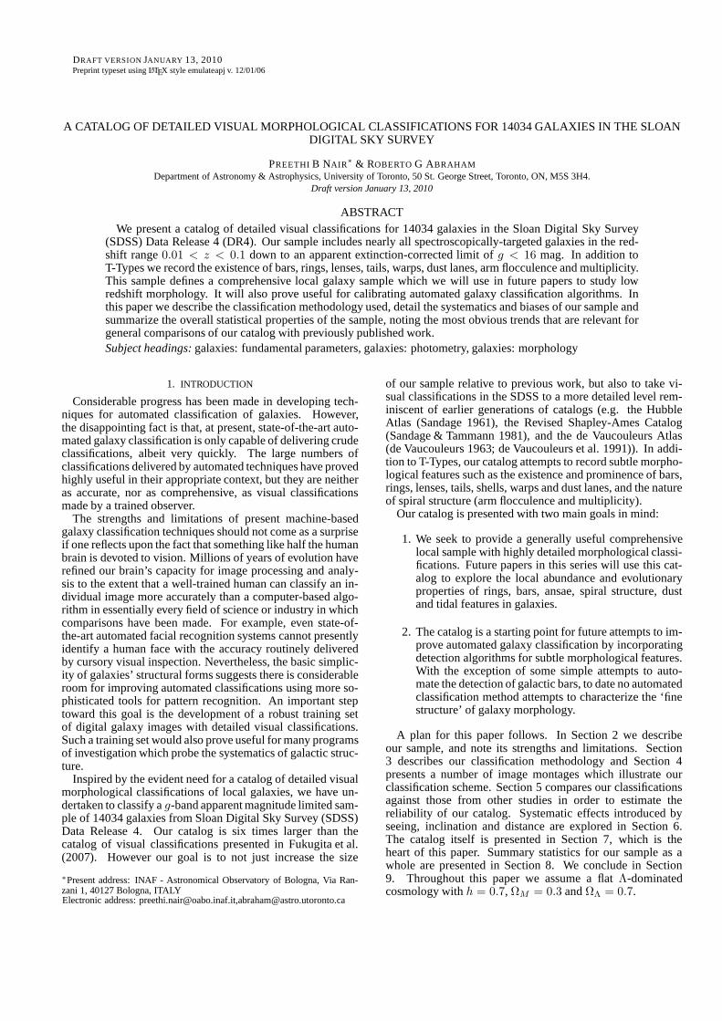
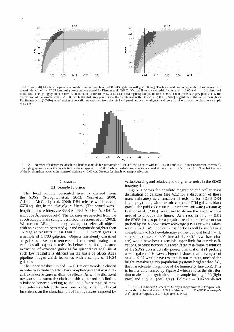


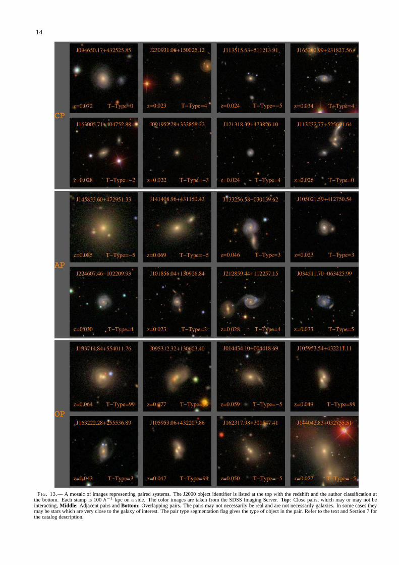


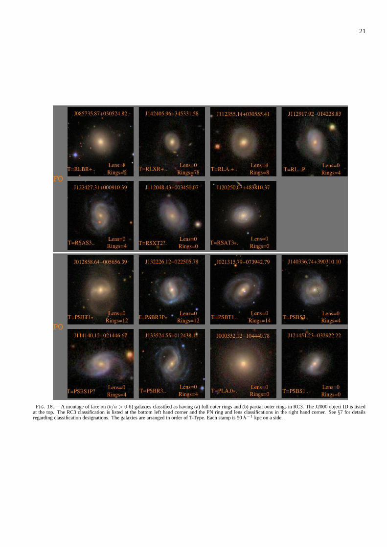
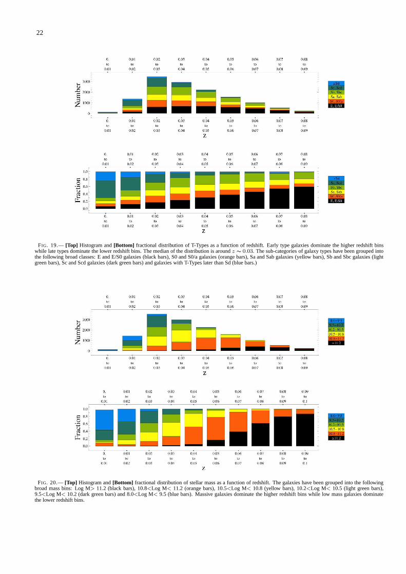


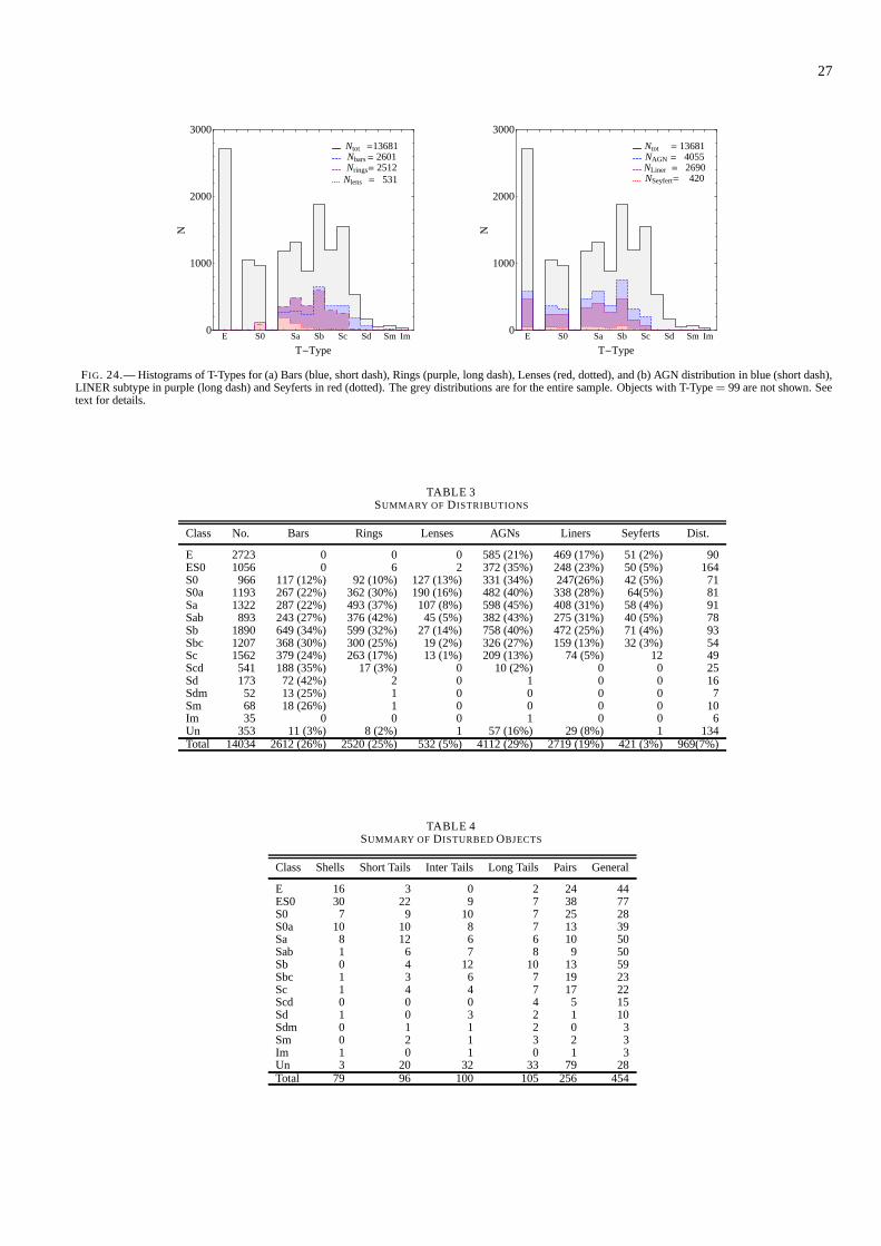

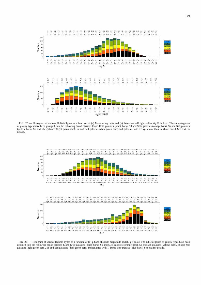


![ljB'tLo -On]S6«f]lgs sf/f]af/ P]g, @)^# @)^#.*.@@ @)^# ;fnsf] P]g g= … · 1 ljB'tLo -On]S6«f]lgs_ sf/f]af/ P]g, @)^# k|df0fLs/0f / k|sfzg ldlt @)^#.*.@@ @)^# ;fnsf] P]g g= g @&](https://static.documents.pub/doc/80x56/606540b646da0f1f720b0aa8/ljbtlo-ons6flgs-sffaf-pg-fnsf-pg-g-1-ljbtlo.jpg)


