p-Causality: Identifying Spatiotemporal Causal Pathwaysfor Air Pollutants with Urban Big Data

Julie Yixuan Zhu1,3,∗ Chao Zhang2,3,∗ Huichu Zhang2,4 Shi Zhi2 Victor O.K. Li1Jiawei Han2 Yu Zheng3,+

1Department of Electrical and Electronic Engineering, the University of Hong Kong, HK2Dept. of Computer Science, University of Illinois at Urbana-Champaign, Urbana, IL, USA

3Microsoft Research Asia, Beijing, China4Apex Data & Knowledge Management Lab, Shanghai Jiao Tong University, Shanghai.

1{yxzhu,vli}@eee.hku.hk 2{czhang82,shizhi2, hanj}@illinois.edu 3yuzheng@microsoft.com4zhc@apex.sjtu.edu.cn

ABSTRACTMany countries are suffering from severe air pollution. Under-standing how different air pollutants accumulate and propagate iscritical to making relevant public policies. In this paper, we useurban big data (air quality data and meteorological data) to identifythe spatiotemporal (ST) causal pathways for air pollutants. Thisproblem is challenging because: (1) there are numerous noisy andlow-pollution periods in the raw air quality data, which may leadto unreliable causality analysis; (2) for large-scale data in the STspace, the computational complexity of constructing a causal struc-ture is very high; and (3) the ST causal pathways are complex dueto the interactions of multiple pollutants and the influence of en-vironmental factors. Therefore, we present pg-Causality, a novelpattern-aided graphical causality analysis approach that combinesthe strengths of pattern mining and Bayesian learning to efficientlyidentify the ST causal pathways. First, pattern mining helps sup-press the noise by capturing frequent evolving patterns (FEPs) ofeach monitoring sensor, and greatly reduce the complexity by se-lecting the pattern-matched sensors as “causers”. Then, Bayesianlearning carefully encodes the local and ST causal relations with aGaussian Bayesian Network (GBN)-based graphical model, whichalso integrates environmental influences to minimize biases in thefinal results. We evaluate our approach with three real-world datasets containing 982 air quality sensors in 128 cities, in three regionsof China from 01-Jun-2013 to 31-Dec-2016. Results show thatour approach outperforms the traditional causal structure learningmethods in time efficiency, inference accuracy and interpretability.

KeywordsCausality; pattern mining, Bayesian learning; spatiotemporal (ST)big data; urban computing.

*Equal contribution. The first authors were interns supervised by the cor-respondence author in MSRA.

+Correspondence author.

Permission to make digital or hard copies of all or part of this work forpersonal or classroom use is granted without fee provided that copies arenot made or distributed for profit or commercial advantage and that copiesbear this notice and the full citation on the first page. To copy otherwise, torepublish, to post on servers or to redistribute to lists, requires prior specificpermission and/or a fee. Request permissions from Permissions@acm.org.c©20XX ACM X-XXXXX-XX-X/XX/XX.

1. INTRODUCTIONRecent years have witnessed the air pollution problem becoming

a severe environmental and societal issue around the world. Forexample, in 2015, the average concentration of PM2.5 in Beijingis greater than 150, classified as hazardous to human health by theWorld Health Organization, on more than 46 days. On Dec 7th2015, the Chinese government issues the first red alert because ofthe extremely heavy air pollution, leading to suspended schools,closed construction sites, and traffic restrictions. Though manyways have been deployed to reduce the air pollution, the severeair pollution in Beijing has not been significantly alleviated.

Identifying the causalities has become an urgent problem formitigating the air pollution and suggesting relevant public policymaking. Previous research on the air pollution cause identifica-tion mostly relies on chemical receptor [1] or dispersion models[2]. However, these approaches often involve domain-specific datacollection which is labor-intensive, or require theoretical assump-tions that real-world data may not guarantee. Recently, with theincreasingly available air quality data collected by versatile sensorsdeployed in different regions, and pubic meteorological data, it ispossible to analyze the causality of air pollution through a data-driven approach.

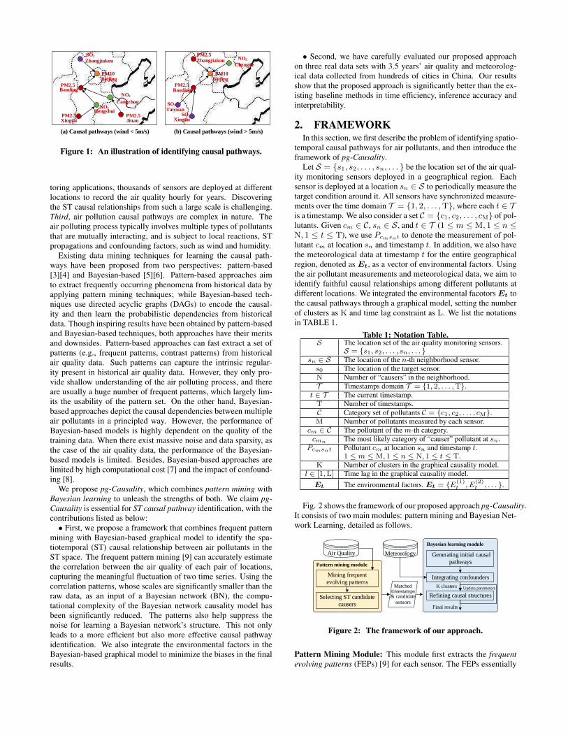
The goal of our research is to learn the spatiotemporal (ST) causalpathways among different pollutants, by mining the dependenciesamong air pollutants under different environmental influences. Fig.1 shows two example causal pathways for PM10 in Beijing. Let usfirst consider the pathway in Fig. 1(a). When the wind speed is lessthan 5 m/s, the high concentration of PM10 in Beijing is mainlycaused by SO2 in Zhangjiakou and PM2.5 in Baoding. In contrast,as shown in Fig. 1(b), when the wind speed is larger than 5m/s,PM10 in Beijing is mainly due to PM2.5 in Zhangjiakou and NO2

in Chengde. Based on this example, we can see the spatiotemporal(ST) causal pathways should reflect the following two aspects: 1)the structural dependency, which indicates the reactions and prop-agations of multiple pollutants in the ST space; and 2) the globalconfounder, which denotes how different environmental conditionscould lead to different causal pathways.

However, identifying the ST causal pathways from big air qual-ity and meteorological data is not trivial because of the followingchallenges. First, not all air pollution data are useful for causal-ity analysis. In the raw sensor-collected air quality data, there arenumerous uninteresting fluctuations and noisy variations. Includ-ing such data into the causality analysis process is expected to leadto unreliable conclusions. Second, the sheer size of the air qualitymakes the causality analysis difficult. In most air quality moni-

arX

iv:1

610.

0704

5v3

[cs

.AI]

18

Apr

201

8

(a) Causal pathways (wind < 5m/s)

NO2

NO2

PM2.5PM2.5

PM2.5

SO2

PM10

(b) Causal pathways (wind > 5m/s)

NO2

SO2

PM2.5

PM2.5

PM10

SO2

Beijing Beijing

Zhangjiakou ZhangjiakouChengde

Baoding

Xingtai

Baoding

Xingtai

Taiyuan

Cangzhou

Hengshui

Jinan

Figure 1: An illustration of identifying causal pathways.

toring applications, thousands of sensors are deployed at differentlocations to record the air quality hourly for years. Discoveringthe ST causal relationships from such a large scale is challenging.Third, air pollution causal pathways are complex in nature. Theair polluting process typically involves multiple types of pollutantsthat are mutually interacting, and is subject to local reactions, STpropagations and confounding factors, such as wind and humidity.

Existing data mining techniques for learning the causal path-ways have been proposed from two perspectives: pattern-based[3][4] and Bayesian-based [5][6]. Pattern-based approaches aimto extract frequently occurring phenomena from historical data byapplying pattern mining techniques; while Bayesian-based tech-niques use directed acyclic graphs (DAGs) to encode the causal-ity and then learn the probabilistic dependencies from historicaldata. Though inspiring results have been obtained by pattern-basedand Bayesian-based techniques, both approaches have their meritsand downsides. Pattern-based approaches can fast extract a set ofpatterns (e.g., frequent patterns, contrast patterns) from historicalair quality data. Such patterns can capture the intrinsic regular-ity present in historical air quality data. However, they only pro-vide shallow understanding of the air polluting process, and thereare usually a huge number of frequent patterns, which largely lim-its the usability of the pattern set. On the other hand, Bayesian-based approaches depict the causal dependencies between multipleair pollutants in a principled way. However, the performance ofBayesian-based models is highly dependent on the quality of thetraining data. When there exist massive noise and data sparsity, asthe case of the air quality data, the performance of the Bayesian-based models is limited. Besides, Bayesian-based approaches arelimited by high computational cost [7] and the impact of confound-ing [8].

We propose pg-Causality, which combines pattern mining withBayesian learning to unleash the strengths of both. We claim pg-Causality is essential for ST causal pathway identification, with thecontributions listed as below:• First, we propose a framework that combines frequent pattern

mining with Bayesian-based graphical model to identify the spa-tiotemporal (ST) causal relationship between air pollutants in theST space. The frequent pattern mining [9] can accurately estimatethe correlation between the air quality of each pair of locations,capturing the meaningful fluctuation of two time series. Using thecorrelation patterns, whose scales are significantly smaller than theraw data, as an input of a Bayesian network (BN), the compu-tational complexity of the Bayesian network causality model hasbeen significantly reduced. The patterns also help suppress thenoise for learning a Bayesian network’s structure. This not onlyleads to a more efficient but also more effective causal pathwayidentification. We also integrate the environmental factors in theBayesian-based graphical model to minimize the biases in the finalresults.

• Second, we have carefully evaluated our proposed approachon three real data sets with 3.5 years’ air quality and meteorolog-ical data collected from hundreds of cities in China. Our resultsshow that the proposed approach is significantly better than the ex-isting baseline methods in time efficiency, inference accuracy andinterpretability.

2. FRAMEWORKIn this section, we first describe the problem of identifying spatio-

temporal causal pathways for air pollutants, and then introduce theframework of pg-Causality.

Let S = {s1, s2, . . . , sn, . . . } be the location set of the air qual-ity monitoring sensors deployed in a geographical region. Eachsensor is deployed at a location sn ∈ S to periodically measure thetarget condition around it. All sensors have synchronized measure-ments over the time domain T = {1, 2, . . . ,T}, where each t ∈ Tis a timestamp. We also consider a set C = {c1, c2, . . . , cM} of pol-lutants. Given cm ∈ C, sn ∈ S, and t ∈ T (1 ≤ m ≤ M, 1 ≤ n ≤N, 1 ≤ t ≤ T), we use Pcmsnt to denote the measurement of pol-lutant cm at location sn and timestamp t. In addition, we also havethe meteorological data at timestamp t for the entire geographicalregion, denoted as Et, as a vector of environmental factors. Usingthe air pollutant measurements and meteorological data, we aim toidentify faithful causal relationships among different pollutants atdifferent locations. We integrated the environmental facotorsEt tothe causal pathways through a graphical model, setting the numberof clusters as K and time lag constraint as L. We list the notationsin TABLE 1.

Table 1: Notation Table.S The location set of the air quality monitoring sensors.

S = {s1, s2, . . . , sn, . . . }sn ∈ S The location of the n-th neighborhood sensor.s0 The location of the target sensor.N Number of “causers” in the neighborhood.T Timestamps domain T = {1, 2, . . . ,T}.

t ∈ T The current timestamp.T Number of timestamps.C Category set of pollutants C = {c1, c2, . . . , cM}.M Number of pollutants measured by each sensor.

cm ∈ C The pollutant of the m-th category.cmn The most likely category of “causer” pollutant at sn.

Pcmsnt Pollutant cm at location sn and timestamp t.1 ≤ m ≤ M, 1 ≤ n ≤ N, 1 ≤ t ≤ T.

K Number of clusters in the graphical causality model.l ∈ [1,L] Time lag in the graphical causality model.

Et The environmental factors. Et = {E(1)t , E

(2)t , . . . }.

Fig. 2 shows the framework of our proposed approach pg-Causality.It consists of two main modules: pattern mining and Bayesian Net-work Learning, detailed as follows.

Mining frequent

evolving patterns

Selecting ST candidate

causers

Integrating confounders

Refining causal structures

K clusters

Bayesian learning module

Pattern mining module

Generating initial causal

pathways

Air Quality Meteorology

Update parametersMatchedtimestamps& candidate

sensorsFinal results

Figure 2: The framework of our approach.

Pattern Mining Module: This module first extracts the frequentevolving patterns (FEPs) [9] for each sensor. The FEPs essentially

capture the air quality changing behaviors that frequently appear onthe target sensor. By mining all FEPs from the historical air qual-ity data, this module efficiently captures the regularity in raw dataand largely reduces the noise (Section 3.1 and 3.2). Afterwards, weexamine the pattern-based similarities between locations to selectcandidate causers for each target sensor. By comparing the FEPsoccurring on different sensors, we can obtain a shallow understand-ing of the causal relationships between different sensors, which canbe further utilized to simplify learning the causal structures (Sec-tion 3.3).

Bayesian Learning Module: By using the matched timestampsof the extracted FEPs at different sensors, together with the se-lected candidate sensors in the pattern mining module, this mod-ule further trains high-quality causal pathways from the large-scaleair quality and context data in an effective and scalable way. Wefirst generate the initial causal pathways from the selected candi-date causers, taking into account both the local interactions of mul-tiple air pollutants and the ST propagations (Section 4.1). Then tominimize the impact of confounding (Section 4.2), we integrate theconfounders (e.g., wind, humidity) into the a Gaussian BayesianNetwork (GBN)-based graphical model. Last, we refine the param-eters and structures of the Bayesian network to generate the finalcausal pathways (Section 4.3).

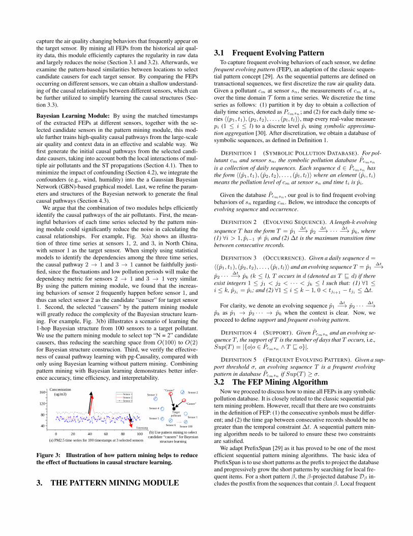
We argue that the combination of two modules helps efficientlyidentify the causal pathways of the air pollutants. First, the mean-ingful behaviors of each time series selected by the pattern min-ing module could significantly reduce the noise in calculating thecausal relationships. For example, Fig. 3(a) shows an illustra-tion of three time series at sensors 1, 2, and 3, in North China,with sensor 1 as the target sensor. When simply using statisticalmodels to identify the dependencies among the three time series,the causal pathway 2 → 1 and 3 → 1 cannot be faithfully justi-fied, since the fluctuations and low pollution periods will make thedependency metric for sensors 2 → 1 and 3 → 1 very similar.By using the pattern mining module, we found that the increas-ing behaviors of sensor 2 frequently happen before sensor 1, andthus can select sensor 2 as the candidate “causer” for target sensor1. Second, the selected “causers” by the pattern mining modulewill greatly reduce the complexity of the Bayesian structure learn-ing. For example, Fig. 3(b) illlustrates a scenario of learning the1-hop Bayesian structure from 100 sensors to a target pollutant.We use the pattern mining module to select top “N = 2” candidatecausers, thus reducing the searching space from O(100) to O(2)for Bayesian structure construcion. Third, we verify the effective-ness of causal pathway learning with pg-Causality, compared withonly using Bayesian learning without pattern mining. Combiningpattern mining with Bayesian learning demonstrates better infer-ence accuracy, time efficiency, and interpretability.

(b) Use pattern mining to select

candidate causers for Bayesian

structure learning(a) PM2.5 time series for 100 timestamps at 3 selected sensors

0 20 40 60 80 100

40

60

80

100

120

140

160

Concentr

ation (

ug/m

3)

Timestamp

Sensor 1

Sensor 2

Sensor 3

Target

pollutant

Causer

Causer

Sensor 1

Sensor 2Sensor 3

Sensor 4

Sensor 5

Sensor 6Sensor 100

...

0 20 40 60 80 100

40

80

120

160 Concentration

(ug/m3)

Figure 3: Illustration of how pattern mining helps to reducethe effect of fluctuations in causal structure learning.

3. THE PATTERN MINING MODULE

3.1 Frequent Evolving PatternTo capture frequent evolving behaviors of each sensor, we define

frequent evolving pattern (FEP), an adaption of the classic sequen-tial pattern concept [29]. As the sequential patterns are defined ontransactional sequences, we first discretize the raw air quality data.Given a pollutant cm at sensor sn, the measurements of cm at snover the time domain T form a time series. We discretize the timeseries as follows: (1) partition it by day to obtain a collection ofdaily time series, denoted as Pcmsn ; and (2) for each daily time se-ries 〈(p1, t1), (p2, t2), . . . , (pl, tl)〉, map every real-value measurepi (1 ≤ i ≤ l) to a discrete level pi using symbolic approxima-tion aggregation [30]. After discretization, we obtain a database ofsymbolic sequences, as defined in Definition 1.

DEFINITION 1 (SYMBOLIC POLLUTION DATABASE). For pol-lutant cm and sensor sn, the symbolic pollution database Pcmsnis a collection of daily sequences. Each sequence d ∈ Pcmsn hasthe form 〈(p1, t1), (p2, t2), . . . , (pl, tl)〉 where an element (pi, ti)means the pollution level of cm at sensor sn and time ti is pi.

Given the database Pcmsn , our goal is to find frequent evolvingbehaviors of sn regarding cm. Below, we introduce the concepts ofevolving sequence and occurrence.

DEFINITION 2 (EVOLVING SEQUENCE). A length-k evolvingsequence T has the form T = p1

∆t−→ p2∆t−→ · · · ∆t−→ pk, where

(1) ∀i > 1, pi−1 6= pi and (2) ∆t is the maximum transition timebetween consecutive records.

DEFINITION 3 (OCCURRENCE). Given a daily sequence d =

〈(p1, t1), (p2, t2), . . . , (pl, tl)〉 and an evolving sequence T = p1∆t−→

p2 · · ·∆t−→ pk (k ≤ l), T occurs in d (denoted as T v d) if there

exist integers 1 ≤ j1 < j2 < · · · < jk ≤ l such that: (1) ∀1 ≤i ≤ k, pji = pi; and (2) ∀1 ≤ i ≤ k − 1, 0 < tji+1 − tji ≤ ∆t.

For clarity, we denote an evolving sequence p1∆t−→ p2 · · ·

∆t−→pk as p1 → p2 · · · → pk when the context is clear. Now, weproceed to define support and frequent evolving pattern.

DEFINITION 4 (SUPPORT). Given Pcmsn and an evolving se-quence T , the support of T is the number of days that T occurs, i.e.,Sup(T ) = |{o|o ∈ Pcmsn ∧ T v o}|.

DEFINITION 5 (FREQUENT EVOLVING PATTERN). Given a sup-port threshold σ, an evolving sequence T is a frequent evolvingpattern in database Pcmsn if Sup(T ) ≥ σ.3.2 The FEP Mining Algorithm

Now we proceed to discuss how to mine all FEPs in any symbolicpollution database. It is closely related to the classic sequential pat-tern mining problem. However, recall that there are two constraintsin the definition of FEP: (1) the consecutive symbols must be differ-ent; and (2) the time gap between consecutive records should be nogreater than the temporal constraint ∆t. A sequential pattern min-ing algorithm needs to be tailored to ensure these two constraintsare satisfied.

We adapt PrefixSpan [29] as it has proved to be one of the mostefficient sequential pattern mining algorithms. The basic idea ofPrefixSpan is to use short patterns as the prefix to project the databaseand progressively grow the short patterns by searching for local fre-quent items. For a short pattern β, the β-projected database Dβ in-cludes the postfix from the sequences that contain β. Local frequent

items in Dβ are then identified and appended to β to form longerpatterns. Such a process is repeated recursively until no more localfrequent items exist. One can refer to [29] for more details.

Given a sequence α and a frequent item p, when creating p-projected database, the standard PrefixSpan procedure generatesone postfix based on the first occurrence of p in α. This strategy,unfortunately, can miss FEPs in our problem.

Table 2: An example symbolic pollution database.Day Daily sequenced1 〈(p2, 0), (p1, 10), (p2, 30), (p3, 40)〉d2 〈(p1, 0), (p2, 30), (p1, 360), (p2, 400), (p3, 420)〉d3 〈(p2, 0), (p3, 30)〉d4 〈(p1, 0), (p1, 120), (p3, 140), (p2, 150), (p3, 180)〉d5 〈(p2, 50), (p2, 80), (p3, 120), (p1, 210)〉

EXAMPLE 1. Let ∆t = 60 and σ = 3. In the database shownin TABLE 2, item p1 is frequent. The p1-projected database gener-ated by PrefixSpan is:

(1) d1/p1 = 〈(p2, 20), (p3, 30)〉(2) d2/p1 = 〈(p2, 30), (p1, 360), (p2, 400), (p3, 420)〉(3) d4/p1 = 〈(p1, 120), (p3, 140), (p2, 150), (p3, 180)〉

The elements satisfying t ≤ 60 are (p2, 20), (p3, 30) and (p2, 30).No local item is frequent, hence p1 cannot be grown any more.

To overcome this, given a sequence α and a frequent item p, wegenerate a postfix for every occurrence of p.

EXAMPLE 2. Also for Example 1, if we generate a postfix forevery occurrence of p1, the p1-projected database is:

(1) d1/p1 = 〈(p2, 20), (p3, 30)〉(2) d2/p1 = 〈(p2, 30), (p1, 360), (p2, 400), (p3, 420)〉(3) d2/p1 = 〈(p2, 40), (p3, 60)〉(4) d4/p1 = 〈(p1, 120), (p3, 140), (p2, 150), (p3, 180)〉(5) d4/p1 = 〈(p3, 20), (p2, 30), (p3, 60)〉

The items p2 and p3 are frequent and meanwhile satisfy the tempo-ral constraint, thus longer patterns p1

60−→ p2 and p160−→ p3 are

found in the projected database.

Using the above projection principle, the projected database in-cludes all postfixes to avoid missing patterns under the time con-straint. Algorithm 1 sketches our algorithm for mining FEPs. Theprocedure is similar to the standard PrefixSpan algorithm in [29],except that the aforementioned full projection principle is adopted,and the time constraint ∆t is checked when searching for local fre-quent items.

Figure 4: An illustration of the pattern-matched timestamps.The blue dashed lines represents the PM2.5 time series in Bei-jing during a two-year period, and the red points denote thetimestamps at which a certain FEP has occurred (σ = 0.1).

Algorithm 1: Mining frequent evolving patterns.Input: support threshold σ, temporal constraint ∆t, symbolic

pollution database P1 Procedure InitialProjection(P , σ, ∆t)2 ← frequent items in D;3 foreach item i in do4 S ← φ;5 foreach sequence o in P do6 R← postfixes for all occurrences of i in o;7 S ← S ∪R;

8 PrefixSpan(i, i, 1, S, ∆t);

9 Function PrefixSpan(α, iprev , l, S|α, ∆t)10 ← frequent items in S|α meeting time constraint ∆t;11 foreach item i in do12 if i 6= iprev then13 α′ ← append i to α;14 Build S|α′ using full projection;15 Output α′;16 PrefixSpan(α′, i, l + 1, S|α′ , ∆t);

The output of Algorithm 1 is the set of all FEPs for the givendatabase, along with the occurring timestamps for each FEP. As anexample, Fig. 4 shows the raw PM2.5 time series in Beijing duringa two-year period. After mining FEPs on the symbolic pollutiondatabase, we mark the timestamps at which the FEPs occur. Onecan observe that, the FEPs can effectively capture the regularly ap-pearing evolvements of PM2.5 in Beijing. Because of the supportthreshold and the evolving constraint, infrequent sudden changesand uninteresting fluctuations are all suppressed.

3.3 Finding Candidate CausersAfter discovering the FEPs, next step is leverage them to extract

the candidate causers for each sensor. Consider two sensors s ands′, let us use TS(s) and TS(s′) to denote the sets of pattern start-ing timestamps for s and s′, respectively. Below, we introduce thepattern match relationship.

DEFINITION 6 (PATTERN MATCH). Let ts′ ∈ TS(s′) be atimestamp at which a pattern happens on s′. For a pattern startingtimestamp ts ∈ TS(s), we say ts′ matches ts if 0 ≤ ts − ts′ ≤ L,where L is a pre-specified time lag threshold.

Informally, the pattern match relation states that when there isa pattern occurring on s′, then within some time interval, there isanother pattern happening on s. Naturally, if s′ has a strong causaleffect on s, then most timestamps in TSs′ will be matched by TSs,and vice versa. Based on TSs and TSs′ , we proceed to introducematch precision and match recall to quantify the correlation be-tween s and s′.

DEFINITION 7 (MATCH PRECISION). Given TSs and TSs′ ,we define the matched timestamp set of TSs′ as Ms′ = {ts′ |ts′ ∈TSs′∧∃ts ∈ TSs,match(ts, ts′) = True}.WithMs′ and TSs′ ,we define the precision of s′ matching s as:

P (s, s′) = |Ms′ |/|TSs′ |

DEFINITION 8 (MATCH RECALL). Given TSs and TSs′ , wedefine the matched timestamp set of TSs asMs = {ts|ts ∈ TSs∧∃ts′ ∈ TSs′ ,match(ts, ts′) = True}. With Ms and TSs, wedefine the recall of s′ matching s as:

R(s, s′) = |Ms|/|TSs|

Relying on the concepts of match precision and match recall, wecompute the pattern-based correlation between s and s′ as:

Corr(s, s′) =2× P (s, s′)

P (s, s′) +R(s, s′).

Now we are ready to describe the process of finding candidatecausers for each sensor. Given the set of all sensors and theirpattern-starting timestamps, our goal is to find the candidate causersfor each sensor. Consider a target sensor s, we say another sensors′ is a candidate causer for s if s′ satisfies two constraints: (1) thedistance between s and s′ is no larger than a distance threshold δg;and (2) the pattern correlation between s and s′ is no less than acorrelation threshold δp. Given the pattern-starting timestamps thatare ordered chronologically, the retrieval of the candidate causerscan be easily done by sequentially scanning the two timestamp liststo find pattern-matched pairs.

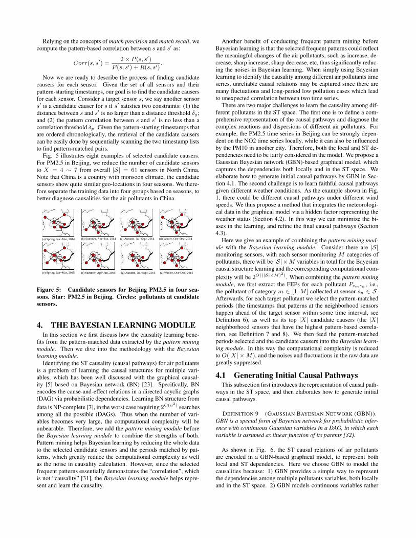
Fig. 5 illustrates eight examples of selected candidate causers.For PM2.5 in Beijing, we reduce the number of candidate sensorsto X = 4 ∼ 7 from overall |S| = 61 sensors in North China.Note that China is a country with monsoon climate, the candidatesensors show quite similar geo-locations in four seasons. We there-fore separate the training data into four groups based on seasons, tobetter diagnose causalities for the air pollutants in China.

(a) Spring, Jan~Mar, 2014

(e) Spring, Jan~Mar, 2015 (f) Summer, Apr~Jun, 2015 (g) Autumn, Jul~Sept, 2015 (a) Winter, Oct~Dec, 2015

(b) Summer, Apr~Jun, 2014 (c) Autumn, Jul~Sept, 2014 (d) Winter, Oct~Dec, 2014

Figure 5: Candidate sensors for Beijing PM2.5 in four sea-sons. Star: PM2.5 in Beijing. Circles: pollutants at candidatesensors.

4. THE BAYESIAN LEARNING MODULEIn this section we first discuss how the causality learning bene-

fits from the pattern-matched data extracted by the pattern miningmodule. Then we dive into the methodology with the Bayesianlearning module.

Identifying the ST causality (causal pathways) for air pollutantsis a problem of learning the causal structures for multiple vari-ables, which has been well discussed with the graphical causal-ity [5] based on Bayesian network (BN) [23]. Specifically, BNencodes the cause-and-effect relations in a directed acyclic graphs(DAG) via probabilistic dependencies. Learning BN structure fromdata is NP-complete [7], in the worst case requiring 2O(n2) searchesamong all the possible (DAGs). Thus when the number of vari-ables becomes very large, the computational complexity will beunbearable. Therefore, we add the pattern mining module beforethe Bayesian learning module to combine the strengths of both.Pattern mining helps Bayesian learning by reducing the whole datato the selected candidate sensors and the periods matched by pat-terns, which greatly reduce the computational complexity as wellas the noise in causality calculation. However, since the selectedfrequent patterns essentially demonstrates the “correlation”, whichis not “causality” [31], the Bayesian learning module helps repre-sent and learn the causality.

Another benefit of conducting frequent pattern mining beforeBayesian learning is that the selected frequent patterns could reflectthe meaningful changes of the air pollutants, such as increase, de-crease, sharp increase, sharp decrease, etc, thus significantly reduc-ing the noises in Bayesian learning. When simply using Bayesianlearning to identify the causality among different air pollutants timeseries, unreliable causal relations may be captured since there aremany fluctuations and long-period low pollution cases which leadto unexpected correlation between two time series.

There are two major challenges to learn the causality among dif-ferent pollutants in the ST space. The first one is to define a com-prehensive representation of the causal pathways and diagnose thecomplex reactions and dispersions of different air pollutants. Forexample, the PM2.5 time series in Beijing can be strongly depen-dent on the NO2 time series locally, while it can also be influencedby the PM10 in another city. Therefore, both the local and ST de-pendencies need to be fairly considered in the model. We propose aGaussian Bayesian network (GBN)-based graphical model, whichcaptures the dependencies both locally and in the ST space. Weelaborate how to generate initial causal pathways by GBN in Sec-tion 4.1. The second challenge is to learn faithful causal pathwaysgiven different weather conditions. As the example shown in Fig.1, there could be different causal pathways under different windspeeds. We thus propose a method that integrates the meteorologi-cal data in the graphical model via a hidden factor representing theweather status (Section 4.2). In this way we can minimize the bi-ases in the learning, and refine the final causal pathways (Section4.3).

Here we give an example of combining the pattern mining mod-ule with the Bayesian learning module. Consider there are |S|monitoring sensors, with each sensor monitoring M categories ofpollutants, there will be |S|×M variables in total for the Bayesiancausal structure learning and the corresponding computational com-plexity will be 2O((|S|×M)2). When combining the pattern miningmodule, we first extract the FEPs for each pollutant Pcmsn , i.e.,the pollutant of category m ∈ [1,M ] collected at sensor sn ∈ S.Afterwards, for each target pollutant we select the pattern-matchedperiods (the timestamps that patterns at the neighborhood sensorshappen ahead of the target sensor within some time interval, seeDefinition 6), as well as its top |X| candidate causers (the |X|neighborhood sensors that have the highest pattern-based correla-tion, see Definition 7 and 8). We then feed the pattern-matchedperiods selected and the candidate causers into the Bayesian learn-ing module. In this way the computational complexity is reducedtoO(|X| ×M), and the noises and fluctuations in the raw data aregreatly suppressed.

4.1 Generating Initial Causal PathwaysThis subsection first introduces the representation of causal path-

ways in the ST space, and then elaborates how to generate initialcausal pathways.

DEFINITION 9 (GAUSSIAN BAYESIAN NETWORK (GBN)).GBN is a special form of Bayesian network for probabilistic infer-ence with continuous Gaussian variables in a DAG, in which eachvariable is assumed as linear function of its parents [32].

As shown in Fig. 6, the ST causal relations of air pollutantsare encoded in a GBN-based graphical model, to represent bothlocal and ST dependencies. Here we choose GBN to model thecausalities because: 1) GBN provides a simple way to representthe dependencies among multiple pollutants variables, both locallyand in the ST space. 2) GBN models continuous variables rather

than discrete values. Due to the sensors monitor the concentra-tion of pollutants per hour, GBN could help better capture the fine-grained knowledge through the dependencies of these continuousvalues. In this subsection, based on the extracted matched pat-terns and candidate sensors from the pattern mining module foreach pollutant Pcmsn , we use Pcmsn to represent continuous val-ues in the graphical model. 3) The characteristics of urban datafit the GBN model well. As shown in Fig. 7, the distribution of1-hour difference (current value minus the value 1-hour ago) of airpollutants and meteorological data obey Gaussian distribution (ver-ified by D′Agostino − Pearson test [33][34]). In the followingsections, normalized 1-hour differences of time series data will beused as inputs for the model.

(a) Local and ST dependencies in a GBN

Q(s1~sN)tST

= { }Pcmsn(t-l)

m in [1,2,...M];

l = 1,2,...L;

Qs0tLocal

= { }Pcms0(t-l)

n = 1,2,...,N

(b) Notations

X1 Pcms0t

L×(N+1)

Qs0tLocal

Q(s1~sN)tST

Geospace

Figure 6: GBN-based causal pathway representation and itsnotations.

0

150

0

0

0 5 0 5 0 5

0 5 0 5 0 5

600

100

-1 0 0 4 01 2 3 2 840

100

0

0

150

40

0

400

0

0

300

60PM2.5 PM10 NO2

CO O3 SO2

Temperature

(T)

Humidity (U) Wind Speed

(WS)

0

1000

0

0

3000

150

20

300

0

0

300

150

0

1000

0

0

1000

150PM2.5 PM10 NO2

CO O3 SO2

Temperature

(T)

Humidity (U) Wind Speed

(WS)

-2 20 -2 20 -2 20

-2 20 -2 20 -2 20

-2 0 -2 20 -2 20

(b) Value of 1-hour difference normalized by

standard deviation

(a) Original values normalized by standard

deviation

Figure 7: Histograms of urban data (original vs. 1-hour dif-ference)

Specifically, for the target pollutant cm at sensor s0-th sensorand timestamp t, denoted as Pcms0t,m ∈ [1,M], we capture thedependencies from both the local causal pollutants QLocal

s0t andthe ST causal pollutants QST

(s1∼sN )t. Here QST(s1∼sN )t refer to

a 1×NL vector of pollutants at N neighborhood sensors s1 ∼ sNand previous L timestamps that most probably cause the target pol-lutant in the ST space, i.e. QST

(s1∼sN )t = {Pcmnsn(t−l)},m ∈[1, . . . ,M];n = 1, . . . ,N; l = 1, . . . ,L. In order to better trace themost likely “causers” spatially, we just preserve the one category ofpollutant at each neighborhood sensor that most influences the tar-get pollutant. We use cmn to represent the category for the mostlikely “causers” at sensor n. Similarly,QLocal

s0t is a 1×ML vectorof pollutants locally at s0. For example, when we set L = 2,M =6,QLocal

s0t may take values of 12 normalized 1-hour difference timeseries data, i.e. QLocal

s0t = (2,−0.5, 0.8, 0.3, 1,−2, 2.2, 1, 1, 0,−0.5, 0.2).The parents ofPcms0t are denoted asPA(Pcms0t) = QLocal

s0t ⊕QST

(s1∼sN )t, where ⊕ denotes the concatenation operator for twovectors. Based on the definition of GBN, the distribution of Pcms0tconditioned on PA(Pcms0t) obeys Gaussian distribution:

Pr(Pcms0t = pcms0t|PA(Pcms0t)) ∼ N (µcms0t+

ΣNn=0ΣL

l=1amn(nL+l)(pcmsn(t−l) − µcmsn(t−l)),Σ(εcms0t))(1)

µcms0t is the marginal mean for Pcms0t. Σ denotes the covari-ance operator. A = {amn(nL + l)}, (mn ∈ [1, . . . ,M];n =0, 1, . . . ,N; l = 1, . . . ,L) is the coefficient for the linear regres-sion in GBN [32]:

To minimize the uncertainty of Pcms0t given its parents, we needto find N sensors s1 ∼ sN from the ST space and the parametersA that minimize the error:

Σ(εcms0t) = Σ(Pcms0t)−AΣ(PA(Pcms0t))−1AT (2)

Generating the initial causal pathways requires locating N mostinfluential sensors from |S| sensors with up to

(|S|N

)trials. Yet

given the candidate sensors selected by Section 3.3, we manage tosearch from a subset (X ≤ |S|) sensors with time efficiency andscalability. We further propose a Granger causality score GCscoreto generate initial causal pathways, which is defined as:

GCscore(m, s0, sn) = maxmn∈[1,M]maxl∈[1,L]

{|match(t(cm,s0), t(cmn ,sn))| ·|Σ(εcms0(t−l))1| − |Σ(εcms0(t−l))2|

|Σ(εcms0(t−l))2|χ2L(0.05)

}

(3)

where GCscore is a χ2-test score [21] for the predictive causality,with higher score indicating more probable “Granger” causes fromM pollutants at sensor sn to the target pollutant cm at sensor s0

[17] (GCscore ≤ 1 means none causality). For variables obey-ing Gaussian distribution, Granger causality is in the same formas conditional mutual information [20], which has been used suc-cessfully for constructing structures for Bayesian networks. Here|match(t(cm,s0), t(cmn ,sn))| is the number of matched timestampsof FEPs between two time series (pollutant cmn at sensor sn andpollutant cm at sensor s0, see Section 3.3). And Σ(εcms0(t−l))1

and Σ(εcms0(t−l))2 correspond to the variances of the target pollu-tantPcms0t conditioned on lagged sequencesQLocal

s0(t−l) andQLocals0(t−l)⊕

QSTsn(t−l).

4.2 Integrating ConfoundersRecall the example in Fig. 1. A target pollutant is likely to

have several different causal pathways under different environmen-tal conditions, which indicate the causal pathways we learn maybe biased and may not reflect the real reactions or propagations ofpollutants. To overcome this, it is necessary to model the environ-mental factors (humidity, wind, etc.) as extraneous variables in thecausality model, which simultaneously influence the cause and ef-fect. For example, when the wind speed is less than 5m/s, city A’sPM2.5 could be the “cause” of city B’s PM10. However, when thewind speed is more than 5m/s, there may not be causal relationsbetween the two pollutants in the two cities. In this subsection,we will elaborate how to integrate the environmental factors intothe GBN-based graphical model, to minimize the biases in causal-ity analysis and guarantee the causal pathways are faithful for thegovernment’s decision making. We first introduce the definition ofconfounder and then elaborate the integration.

DEFINITION 10 (CONFOUNDER). A confounder is defined asa third variable that simultaneously correlates with the cause andeffect, e.g. gender K may affect the effect of recovery P given amedicine Q, as shown in Fig. 8(a). Ignoring the confounders willlead to biased causality analysis. To guarantee an unbiased causalinference, the cause-and-effect is usually adjusted by averagingall the sub-classification cases of K [5], i.e. Pr(P |do(Q)) =ΣKk=1Pr(P |Q, k)Pr(k).

Q P

K

Cause

(e.g. medicine)

Effect

(e.g. recovery)

Confounding

variable (e.g.

gender)

X1

(a) Cause-and-effect with confounder

Pcms0t

L×(N+1)×M

Qs0tLocal

Q(s1~sN)tST

Qt={...} Pt

K

Environmental factors (e.g.

meteorology)

Geospace

Qt Pt

Markov equivalence

K

Et

(b) An illustration of cause-and-effect with confounders (environmental factors)

integrating into a hidden variable K, for causality analysis

Et={Et, Et, Et, }

Geospace

Qt Pt

K

Et

π

(c) Learn K labels for Pt, Qt, Et via

a generative model

For each target pollutant cm at sensor s0

(1) (2) (3)

Figure 8: The GBN-based graphical model, integrating con-founders to the causal pathway, and converting the model intoa generative model

For integrating environmental factors as confounders, denotedas Et = {E(1)

t , E(2)t , . . . }, into the GBN-based causal pathways,

one challenge is there can be too many sub-classifications of en-vironmental statuses. For example, if there are 5 environmentalfactors and each factor has 4 statuses, there will exist 45 = 1024causal pathways for each sub-classification case. Directly integrat-ing Et as confounders to the cause and effect will result in unre-liable causality analysis due to very few sample data conditionedon each sub-classification case. Therefore, we introduce a discretehidden confounding variableK, which determines the probabilitiesof different causal pathways fromQt to Pt, as shown in Fig. 8(b).The environmental factors Et are further integrated into K, whereK = 1, 2, ...K. In this ways, the large number of sub-classificationcases of confounders will be greatly reduced to a small number K,as K clusters of the environmental factors.

Based on Markov equivalence (DAGs which share the same jointprobability distribution [35]), we can reverse the arrowEt → K toK → Et, as shown in the right part of Fig. 8(b). K determines thedistributions of P,Qt,Et, thus enabling us to learn the distributionof the graphical model from a generative process. To help us learnthe hidden variable K, the generative process further introducesa hyper-parameter π (as shown in Fig. 8(c)) that determines thedistribution of K. Thus the graphical model can be understood asa mixture model under K clusters. We learn the parameters of thegraphical model by maximizing the new log likelihood:

LLgen = ΣtΣKk=1ln(Pr(pt|qt, k)Pr(et|k)Pr(k|π)) (4)

In determining the number of the hidden variable K, we do notconsider too large K values since that will induce much complexityfor causality analysis. Also a too small K may not characterize theinformation contained in the confounders (i.e. meteorology). Weobserve the 2-D PCA projections of meteorological data (as shownin Fig. 9). In three regions, five clusters can characterize the datasufficiently well. Thus we choose K = 3 ∼ 7 for learning inpractice.

4.3 Refining Causal StructuresThis subsection tries to refine the causal structures and obtain

the final causal structures under K clusters. The refining processincludes two phases in each iteration: 1) an EM learning (EML)phase to infer the parameters of the model, and 2) a structure recon-struction (SR) phase to re-select the top N neighborhood sensors

-350 -300 -250 -200 -150 -100 -5025

30

35

40

45

50

-100 -50 0 50 100 150 200-85

-80

-75

-70

-65

-60

-55

-100 -50 0 50 100 150-165

-160

-155

-150

-145

-140

-135

(a) North China (NC)(b) Yangtze River Delta (YRD) (c) Pearl River Delta (PRD)

25

50

-350 -300 -250 -200 -150 -100 -50

30

35

40

45

-85

-100 -50 0 50 100 150 200

-55

-70

-100 -50 0 50 100 150

-165

-135

-150

(a) North China (NC)

Figure 9: 2-D PCA projections of 5 clusters of meteorologicaldata in NC, YRD and PRD. The original meteorological datacontains five types, i.e. temperature (T), pressure (P), humid-ity (U), wind speed (WS), and wind direction (WD), with eachregion divided into 9 grids, thus 45-dimensional.

based on the newly learnt parameters andGCscore, as illustrated inAlgorithm 2.

EML (line 6-18) is an approximation method to learn the param-eters π, γ,Ak,Bk of the graphical model, by maximizing the loglikelihood (Equation 4) of the observed data sets via an E-step anda M -step. Here π contains the hyper parameters which determinethe distribution of K (T × K-dimensional). γ are posterior proba-bilities for each monitoring record (T×K-dimensional). Ak,Bk

are parameters for measuring the dependencies among pollutantsand meteorology (K-dimensional). Note thatAk,Bk come in dif-ferent formats. Ak is the regression parameter for:

Pcms0t = µ0 + (QLocals0t ⊕QST

(s1∼sN )t)Ak + εcms0t (5)

and Bk = (µBk ,ΣBk) = (mean(Et), std(Et)) includes theparameters for the multivariate Gaussian distribution of environ-mental factors Et. In the E-step, we calculate the expectation oflog likelihood (Equation 6) with the current parameters, and theM -step re-computes the parameters.E-step: Given the parameters π,K,N,Ak,Bk, EM assumes themembership probability γtk, i.e., the probability of pt, qt, et be-longing to the k-th cluster as:

γtk = Pr(k|pt, qt, et) =Pr(k)Pr(pt, qt, et|k)

Pr(pt, qt, et)

=πtkN (pt|qt,Ak)N (et|Bk)

ΣKj=1πtjN (pt|qt,Aj)N (et|Bj)

(6)

M -step: The membership probability γtk in E-step can be usedto calculate new parameter values πnew,Anew

k ,Bnewk . We first

determine the most likely assignment tag of timestamp t to clusterk, i.e.

Tagt = maxk∈[1,K]πtk (7)

By integrating the timestamps belonging to each cluster k, wecan updateAnew

k by Equation 5. Then we updateBk by:

µnewBk

=1

TkΣTt=1γtket, Tk = ΣTt=1γtk

ΣnewBk

=1

TkΣTt=1γtk(et − µnew

Bk)(et − µnew

Bk)T

(8)

In addition, we update πnewtk by:

πnewtk =γtkTk

(9)

The SR phase (line 19-24) utilizes the parameters provided bythe EM learning phase, and re-select the top N neighborhood sen-sors based on the newly generated GCscore for each cluster k. Wepresent a training example (as shown in Fig. 10(a)) of learningthe causal pathways for Beijing PM2.5 during Jan−Mar. After 20training iterations of the EM learning phase and structure recon-struction, we finally obtain K = 4 causal structures under eachcluster, with the log likelihood shown in Fig. 10(b). We find thelog likelihood does not increase much after 10 iterations, thus weset the iteration number to 10 in our experiments. For the last iter-ation, we calculate the percentage of labeled timestamps belongingto each cluster k. In this example, we find that Beijing’s PM2.5is more likely to be influenced by NO2 in Baoding and PM10 inCangzhou.

Algorithm 2: Refining the causal structures for each target pol-lutant cm at location s0.

Input: T,K,N, and raining data sets pt, qt, et, t ∈ [1,T]Output: Refined causal structures for K clusters

1 Initial neighborhood sensors s1 ∼ sN based on top N GCscore;2 repeat3 EML(Pt, Qt, Et, s1 ∼ sN , K)

→ Log_likelihood, πtk, γtk,Ak,Bk;4 SR(Ak, s1 ∼ sN , K)→ s′1 ∼ s′N , Q′;5 until Log_likeoihood converges;6 Function EM_Learning(EML)(Pt, Qt, Et, s1 ∼ sN , K)7 repeat8 InitialAssign: K clusters via K-means(Et)9 foreach item t = 1 to T do

10 foreach item k = 1 to K do11 Update πtk by Equation (9);

12 foreach item k = 1 to K do13 Update Ak,Bk by Equation (5),(8);

14 foreach item t = 1 to T do15 foreach item k = 1 to K do16 Update γtk by Equation (6);

17 until Log likelihood converges;18 return: Log_likelihood and πtk, γtk,Ak,Bk;

19 Function Structure_Reconstruction(SR)(Ak, s1 ∼ sN , K)20 foreach item sn in All candidate sensors do21 Compute GCscore(m, s0, sn) for s1 ∼ sN ;22 Rank GCscore and re-select the top N neighborhood sensors

s′1 ∼ s′N ;23 Update Q→ Q′ corresponding to s′1 ∼ s′N ;

24 return: s′1 ∼ s′N , Q′;

5. EXPERIMENTSWe evaluate the empirical performance of our method in this sec-

tion. All the experiments were conducted on a computer with In-tel Core i5 3.3Ghz CPU and 16GB memory. We use MATLABfor our Bayesian learning module, and the open-source MATLABBNT toolbox [36] for baseline methods.

5.1 Experimental Setup

5.1.1 Data SetsWe use three data sets that contain the records of 6 air pollutants

and 5 meteorological measurements:• North China (NC), with 61 cities, 544 air quality monitoring

sensors and 404 meteorological sensors in North China. The lati-tude and longitude ranges are 34N-43N, 110E-123E.

• Yangtze River Delta (YRD), with 49 cities, 330 air qualitymonitoring sensors and 48 meteorology sensors. The latitude andlongitude ranges are 28N-35N, 115E-123E, respectively.• Pearl River Delta (PRD), with 18 cities, 124 air quality moni-

toring sensors and 406 meteorology sensors. The latitude and lon-gitude ranges are 22N-25N, 110E-116E.

The 6 air pollutants are PM2.5, PM10, NO2, CO, O3, SO2, andthe 5 meteorological measurements are temperature (T), pressure(P), humidity (H), wind speed (WS), and wind direction (WD),which are updated hourly. The time span for all data sets is from01/06/2013 to 31/12/2016. We separate each data set into fourgroups based on four seasons, and use the last 15 days in each sea-son in year 2014, 2015, 2016 for testing, and the remaining data formodel training. The total numbers of training timestamps are 5424,6193, 7753, 7752 in the four seasons, respectively, and the numberof the corresponding testing timestamps is 15×24×3=1080 in eachseason. To get the environmental factorsEt for the coupled model,we divide each region into 3×3 grids and average the meteorologyvalues within each grid.

We conduct experiments at both city level (Section 5.2.2, 5.2.1,5.2.5) and sensor level (Section 5.2.3). The city-level experimentsaverage value of the sensors in the city to form a pseudo sensor, anddiscover the pathways among all the cities in three data sets. Thesensor-level experiments analyze the causal relationships amongsensors in each data set.

5.1.2 BaselinesSince Bayesian-based methods have been well used to learn causal

Bayesian structures [23], we choose the most commonly used BNstructure learning approaches as baselines to compare with our method.To identify the dependencies among different pollutants, the base-lines are deployed to learn the causal structures for each target pol-lutant.1. MWST. Maximum Weighted Spanning Tree (MWST) generatesan undirected tree structure based on the MWST algorithm [37].Each time it connects one edge between two nodes with the max-imum mutual information. Furthermore, [38] proposed an inde-pendency test method to assign a direction to each edge in the treestructure.2. MCMC. Markov-chain Monte Carlo (MCMC) is a statisticalmethod that also samples from the Directed Acyclic Graph (DAG)space [39]. The method maximizes the score from a set of simi-lar DAGs that add, delete, or reverse connections, and updates thestructure in the next iteration.3. K2+PS. K2 is a widely used greedy method for Bayesian struc-ture learning, which selects at most N parents based on the K2score [40] for each variable given the updating order of all the vari-ables. In our case, we use pattern search algorithm [41] to optimizethe updating order, thus reducing the search space of casual path-ways of different pollutants. Note that the original K2 score isdefined for discrete variables. Here we use GCscore instead for thecontinuous variables.4. CGBN. Coupled Gaussian Bayesian network [6] is a data-drivencausality model considering the dependencies between both theair pollutants and meteorology. CGBN assumes there is a thirdvariable (confounder, such as gender as a confounder to evaluatethe effect of a medicine on a disease) which simultaneously influ-ences the dependences among pollutants and among environmen-tal factors, coupling pollutants and environmental factors together.The difference between CGBN and our approach is that 1) our ap-proach integrates the environmental factors directly into the graph-ical model, instead of through coupling, and 2) our approach hasa pattern mining module and a refining algorithm to optimize the

0 5 10 15 20-2.85

-2.8

-2.75

-2.7

-2.65x 10

5

Beijing

Langfang PM10

Tianjin PM10

Initialization

...

Beijing

Beijing

Cangzhou PM10

Beijing

Beijing

Baoding NO2

Initial K

clusters by

kmeansk=3, p=0.2852

k=1, p=0.2165

k=4, p=0.2283

Log

likelihood

converges

Final structures under K clusters

(a) Training process to generate causal pathways under K clusters (b) Log likelihood vs. 20 epochs

Beijing

Zhangjiakou PM10

Beijing

Tianjin SO2

Beijing

Beijing

EML()

SR()

Tangshan PM2.5

k=3

k=1

k=4

k=2

Iteration 1

Structures under K clusters

Beijing

Beijing

Tianjin SO2Baoding

CO

Beijing

Zhangjiakou SO2

Beijing

EML()

SR()

k=3

k=1

k=4

k=2

Iteration 2

Structures under K clusters

Chengde SO2

Chengde PM10

Chengde NO2

Zhangjiakou NO2

Chengde O3

Chengde NO2

Zhangjiakou NO2

Chengde O3

Chengde NO2

Zhangjiakou NO2

k=2, p=0.2701

Zhangjiakou NO2

Langfang NO2

Chengde NO2

Baoding NO2

Langfang PM2.5

Zhangjiakou NO2

Figure 10: An example of learning the causal pathway for PM2.5, Jan−Mar in Beijing under K = 4 clusters.

learning process.

5.1.3 Parameter SettingThe parameters of pg-Causality include: (1) the support thresh-

old σ; (2) the temporal constraint ∆t; (3) the distance threshold δgfor finding candidate causers; and (4) the correlation threshold δpfor finding candidate causers; (5) the number of time lags L = 3; (6)and the number of pollutant categories M = 6. When finding causalpathways at city level, we set σ = 0.1, ∆t = 1 hour, δg = 200km, and δp = 0.5. At the station level, all the the parameters are setthe same except that δg = 15 km to impose a finger granularity forfinding candidate causers. K and N are evaluated within the rangeK = 3 ∼ 7, and N= 1 ∼ 5.

5.2 Experimental ResultsThe verification of causality is a very critical part in causal mod-

elling. The simplest method for evaluating causal dependence is tointervene in a system and determine if the model is accurate un-der intervention. However, substantial and direct intervention in airpollution is impossible. By investigating the verification methodsin previous causality works, we propose five tasks to evaluate theeffectiveness of our approach, namely, 1) inference accuracy for a1-hour prediction task, 2) time efficiency, 3) scalability, 4) verifi-cation on synthetic data, and 5) visualizing the causal pathways.Tasks 1-3 target to evaluate whether the model fits the dependencesamong the datasets well. Task 4 tries to learn the causal pathwaysfor a predefined causal structure generated by synthetic datasets.And Task 5 targets at the interpretability of the causal pathways welearn.

5.2.1 Inference AccuracyWe first evaluate the effectiveness of our approach via the causal

inference accuracy through the causal pathways at city level, whichis a 1-hour prediction task based on our proposed GBN-based graph-ical model. Note this prediction task is not general for all the times-tamps, it only predicts the future 1-hour based on the extractedpattern-matched periods, indicating the causal inference for the fre-quent evolving behaviors. Specifically, we first infer the probabilityPr(k) of the testing data belonging to cluster k. Then, we use thestructure and parameters from the trained causal pathways regard-ing this cluster to estimate the future pollutant concentration byEq. 10.

P estcms0t = ΣKk=1(µ0k + PA(Pcms0t)Ak)Pr(k) (10)

The accuracy is defined as ΣTtestt=1 (P estcms0t−P

∗cms0t)/P

∗cms0tTtest,

where P ∗cms0t is the ground truth value and Ttest is the numberof test cases. TABLE 3 shows the 1-hour prediction accuracy forPM2.5 and PM10 with our approaches pg-Causality, pg-Causality-n, pg-Causality-p, and the three baseline methods in Beijing (Re-gion NC), Shanghai (Region YRD), and Shenzhen (Region PRD).Here pg-Causality-n represents pg-Causality without the pattern

mining module, and pg-Causality-p represents pg-Causality with-out integrating confounders. The accuracy shown in TABLE 3 isthe accuracy for spring for three cities. The pg-Causality gets thehighest accuracy (92.5%, 93.78%, 95.39% for PM2.5 in Beijing,Shanghai, and Shenzhen, respectively; 91.36%, 92.39%, 93.18%for PM10, repectively.), compared to pg-Causality-n and pg-Causality-p, as well as the three baseline methods WMST, K2+PS, and CGBN.We did not include the accuracy of MCMC in TABLE 3 due toits unbearably high computational time. The accuracy for MCMCis lower than 60%, which is not competitive with the other meth-ods mentioned. The highest inference accuracy for the three citiesare marked with three different colors (orange for Beijing, blue forShanghai, and green for Shenzhen) given different parameters Kand N. K and N are obtained based on the maximum inferenceaccuracy for each city. We note N = 2,K = 4 provides the bestperformance for Beijing, while N = 0,K = 5 or 6 generate thebest accuracy for Shanghai and N = 0,K = 1 for Shenzhen. Theoptimal number N = 2 for Beijing also suggests that the air pol-lution is mainly influenced by the most influential sensors in theST space. While the optimal number N = 0 for Shanghai andShenzhen suggests that the PM2.5 in these two cities are mainlyinfluenced by historical pollutants locally.

We also evaluate the 1-hour prediction accuracy with three well-used time series model, i.e., auto-regression moving average (ARMA)model, linear regression model (LR), and support vector machinefor regression with a Gaussian radial basis function (rbf) kernel(represented as SVM-R). Generally, pg-Causality demonstrates higherinference accuracy compared with these time series models, exceptfor the PM2.5 in Shanghai.

5.2.2 Time efficiencyWe also compare the training time of pg-Causality with base-

line methods, as shown in TABLE 4. Since our approach consistsof both pattern mining and Bayesian learning modules, we presentthe averaged time consumption of training all the three data sets,for each step in the two modules. We also evaluate the overalltime consumption of pg-Causality and pg-Causality-n without thepattern mining module (Section 5.1 (p+g) refers to the time cost ofcausal structure initialization with both pattern mining and Grangercausality score. Section 5.1 (g) refers to only using Granger causal-ity score). Results show that our approach is very efficient, with thesecond minimum computation time among all the methods. MWSTconsumes the minimal time, however, it does not generate satisfac-tory accuracy for prediction (as in Section 5.2.1). We thus considerour approach provides the best trade-off regarding accuracy andtime efficiency.

5.2.3 ScalabilityAnother superior characteristic of our approach is the scalabil-

ity. We further identify the causal pathways for air pollutants atsensor level, which is more than ten times as large as in the city-

Table 3: Accuracy of PM2.5/PM10 1-hour prediction vs. baselines, Beijing, Shanghai, and Shenzhen.

Beijing PM2.5, 1-hour prediction accuracy

Shanghai PM2.5, 1-hour prediction accuracy

Shenzhen PM2.5, 1-hour prediction accuracy

Beijing PM10, 1-hour prediction accuracy

Shanghai PM10, 1-hour prediction accuracy

Shenzhen PM10, 1-hour prediction accuracy

Acc

ura

cy

N =

0

N =

1

N =

2

N =

3

N =

4

N =

5

pg-C

au

sali

ty

(Op

tim

al

K,

N)

p

g-C

au

sali

ty-n

p

g-C

au

sali

ty-p

MW

ST

CG

BN

K2+

PS

AR

MA

LR

SV

M-R

K = 1 0.9174 0.9075 0.9067 0.9149 0.9134 0.9132

0.9

25

(K=

4,

N=

2)

0.9

174 (

K=

1,

N=

0)

0.9

105

0.6

91

0.9

236

0.8

01

0.8

756

0.9

048

0.9

157

K = 2 0.9164 0.9059 0.8987 0.9168 0.9180 0.9211

K = 3 0.9162 0.9089 0.9216 0.9177 0.9236 0.9179

K = 4 0.9148 0.9127 0.9250 0.9155 0.9209 0.9216

K = 5 0.9123 0.9214 0.9244 0.9081 0.9198 0.9153

K = 6 0.9144 0.9190 0.9238 0.9195 0.9193 0.9189

K = 7 0.9129 0.9162 0.9157 0.9229 0.9201 0.9201

Acc

ura

cy

N =

0

N =

1

N =

2

N =

3

N =

4

N =

5

pg-C

au

sali

ty

(Op

tim

al

K,

N)

p

g-C

au

sali

ty-n

p

g-C

au

sali

ty-p

MW

ST

CG

BN

K2+

PS

AR

MA

LR

SV

M-R

K = 1 0.8958 0.8936 0.8951 0.9066 0.9035 0.9060

0.9

136

(K=

4,

N=

3)

0.9

003 (

K=

7,

N=

1)

0.8

857

0.6

53

0.9

131

0.8

42

0.8

561

0.8

932

0.8

977

K = 2 0.8989 0.8981 0.8990 0.9070 0.9123 0.9118

K = 3 0.8996 0.8985 0.8992 0.9016 0.9107 0.9094

K = 4 0.8990 0.8984 0.8980 0.9136 0.9111 0.9119

K = 5 0.8995 0.9008 0.9015 0.9059 0.9017 0.9108

K = 6 0.8985 0.9061 0.9061 0.9079 0.9097 0.9095

K = 7 0.8998 0.8991 0.9012 0.9134 0.9096 0.9127

Acc

ura

cy

N =

0

N =

1

N =

2

N =

3

N =

4

N =

5

pg-C

au

sali

ty

(Op

tim

al

K,

N)

p

g-C

au

sali

ty-n

p

g-C

au

sali

ty-p

MW

ST

CG

BN

K2+

PS

AR

MA

LR

SV

M-R

K = 1 0.9375 0.9356 0.9356 0.9356 0.9355 0.9355

0.9

378

(K=

5,

N=

0)

0.9

378 (

K=

1,

N=

0)

0.8

928

0.6

67

0.9

376

0.7

51

0.9

209

0.9

378

0.9

381

K = 2 0.9372 0.9349 0.9359 0.9363 0.9358 0.9332

K = 3 0.9375 0.9373 0.9314 0.9323 0.9327 0.9301

K = 4 0.9377 0.9345 0.9328 0.9296 0.9330 0.9325

K = 5 0.9378 0.9328 0.9339 0.9337 0.9335 0.9263

K = 6 0.9378 0.9328 0.9342 0.9341 0.9315 0.9323

K = 7 0.9372 0.9335 0.9303 0.9316 0.9304 0.9289

Acc

ura

cy

N =

0

N =

1

N =

2

N =

3

N =

4

N =

5

pg-C

au

sali

ty

(Op

tim

al

K,

N)

p

g-C

au

sali

ty-n

p

g-C

au

sali

ty-p

MW

ST

CG

BN

K2+

PS

AR

MA

LR

SV

M-R

K = 1 0.9239 0.9229 0.9232 0.9226 0.9226 0.9227

0.9

239

(K=

1,

N=

0)

0.9

239 (

K=

1,

N=

0)

0.9

173

0.6

31

0.9

239

0.8

35

0.9

042

0.9

238

0.9

239

K = 2 0.9231 0.9212 0.9226 0.9149 0.9204 0.9201

K = 3 0.9228 0.9198 0.9203 0.9194 0.9188 0.9186

K = 4 0.9227 0.9201 0.9172 0.9183 0.9157 0.9174

K = 5 0.9215 0.9199 0.9199 0.9147 0.9183 0.9167

K = 6 0.9226 0.9183 0.9171 0.9187 0.9178 0.9180

K = 7 0.9236 0.9177 0.9170 0.9167 0.9186 0.9154

Acc

ura

cy

N =

0

N =

1

N =

2

N =

3

N =

4

N =

5

pg-C

au

sali

ty

(Op

tim

al

K,

N)

p

g-C

au

sali

ty-n

p

g-C

au

sali

ty-p

MW

ST

CG

BN

K2+

PS

AR

MA

LR

SV

M-R

K = 1 0.9315 0.9307 0.9318 0.9299 0.9296 0.9300

0.9

318

(K=

1,

N=

2)

0.9

315 (

K=

1,

N=

0)

0.9

226

0.6

94

0.9

315

0.8

53

0.0

.95

0.9

250

0.9

275

K = 2 0.9308 0.9291 0.9294 0.9294 0.9290 0.9286

K = 3 0.9309 0.9289 0.9304 0.9289 0.9292 0.9297

K = 4 0.9307 0.9303 0.9311 0.9301 0.9279 0.9286

K = 5 0.9313 0.9307 0.9263 0.9297 0.9302 0.9283

K = 6 0.9303 0.9311 0.9284 0.9282 0.9263 0.9268

K = 7 0.9301 0.9295 0.9305 0.9299 0.9261 0.9254

Acc

ura

cy

N =

0

N =

1

N =

2

N =

3

N =

4

N =

5

pg-C

au

sali

ty

(Op

tim

al

K,

N)

p

g-C

au

sali

ty-n

p

g-C

au

sali

ty-p

MW

ST

CG

BN

K2+

PS

AR

MA

LR

SV

M-R

K = 1 0.9539 -- -- -- -- --

0.9

539

(K=

1,

N=

0)

0.9

54 (

K=

1,

N=

0)

0.9

006

0.6

58

0.9

539

0.7

13

0.9

097

0.9

482

0.9

484

K = 2 0.9533 -- -- -- -- --

K = 3 0.9535 -- -- -- -- --

K = 4 0.9534 -- -- -- -- --

K = 5 0.9532 -- -- -- -- --

K = 6 0.9524 -- -- -- -- --

K = 7 0.9530 -- -- -- -- --

Table 4: Computation time for training data sets at city level.Time (s) m = 1 m = 2 m = 3 m = 4 m = 5 m = 6

Section 4.1 - 4.2 2.74 3.49 3.98 3.74 3.94 3.71

Section 4.3 29.88 43.28 55.15 39.07 45.44 43.13

Section 5.1 (p + g) 73.43 111.33 151.63 94.56 136.64 128.47

Section 5.1 (g) 1125.51 1076.97 1068.13 1074.94 1057.67 1082.85

Section 5.2 -- -- -- -- -- --

Section 5.3 38421.53 42094.47 39137.81 44162.31 49192.68 44601.73

pg-Causality 38527.58 42252.57 39348.57 44299.68 49378.7 44777.04

pg-Causality-n 39547.04 43171.44 40205.94 45237.25 50250.35 45684.58

MWST 6357.9 6529.88 6605.31 7033.58 7216.45 7374.13

CGBN 72785.54 79165.28 80356.3 75578.74 79623.57 78191.32

MCMC 524731.63 562835.19 -- -- -- --

K2 + PS 286592.52 324851.47 -- -- -- --

level analysis. Our approach provides linear scalability in timewith 11.6 hours training time at city level for 128 cities, and 126hours at sensor level for 982 stations. We here claim linear scal-ability since we did not try to find the optimal causal structureby searching the DAG space, which is an NP hard problem andin the worst case requires 2O(n2) searches [7]. In this paper, thecausal pathways we learnt are based on greedy-based approxima-tion. For the structure learning algorithm, we assume the numberof parameters of the Bayesian-based graphical model to be (#), andthe training iterations to be Niter . For totally N sensors in thegeospace and T timestamps in the training records, the time costfor the EM learning (EML) phase is O(Niter × (#) × N × T),assuming every parameter is updated once for every record. In ad-dition, the time cost for the structure reconstruction (SR) phase is

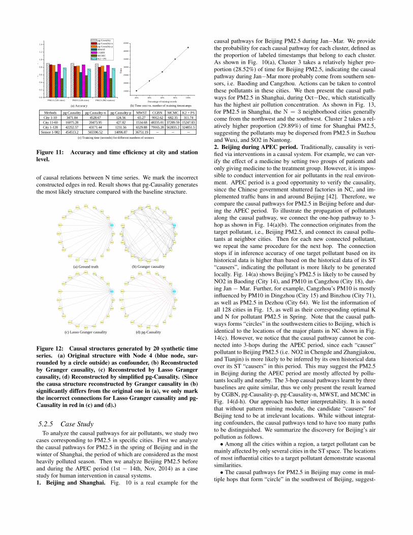
O(Niter × X × L × N × T + Niter × K × (#) × N × T),where X is the candidate “causers” selected by pattern mining andL is the number of time lags. Thus the overall training time isNiterO(XL + (1 + K)(#))NT. If the number of the graphicalmodel (#) is fixed, the computation time will approximately be atlinear scalability with the sensor number N and timestamps num-ber T. We verified the linear scalability in Fig. 11(b)(c). For thebaseline methods, MCMC even cannot compute such large datasets. CGBN and K2 +PS are unable to compute within 10 daysand we leave their time cost as blank, as shown in 11(c). Mean-while, the accuracy is guaranteed when extending city-level data tosensor-level data, as shown in Fig. 11(a).

5.2.4 Verification with Synthetic DataSince the verification of causality via prediction task may not

fully reflect the cause-and-effect relationships learned by the model,we further conduct experiments with synthetic data to judge whetherthe causality identification is correct or not.

As shown in Fig. 12, we generate N = 20 time series, with thepre-defined causal structure as in Fig. 12(a). This is done by ran-domly choosing the lag k for any edge x→ y in the feature causalgraph [22]. To imitate the confounding effect, one time series is se-lected to influence all other time series. We reconstruct the causalstructures through Granger causality (as shown in Fig. 12(b)), lassoGranger causality (as shown in Fig. 12(c) [22]), and pg-Causality(as shown in Fig. 12(d)). To fit pg-Causality in this “toy” model,we simplified the model by randomly assigning locations to N timeseries. In the meanwhile, we set the distance constraint for select-ing candidate “causers” to infinity, in order to consider every pair

PM2.5 (128 cities) PM10 (128 cities) PM2.5 (982 stations)

0.0

0.2

0.4

0.6

0.8

1.0

1.2

1.4

pg-Causality

pg-Causality

pg-Causality-n

pg-Causality-p

MWST

CGBN

MCMC

K2 + PS

Methods pg-Causality pg-Causality-n pg-Causality-p MWST CGBN MCMC K2 + PS

City 1-10 3471.84 4528.67 124.56 65.27 9012.62 682.35 311.74

City 11-60 16075.28 20473.95 427.82 1534.68 48335.01 37289.59 15247.83

City 1-128 42252.57 43171.44 1231.56 6529.88 79165.28 562835.2 324851.5

Sensor 1-982 454513.2 565596.52 14096.87 36751.19 -- -- --

(a) Accuracy (b) Time cos t vs. number of training timestamps

(c) Training time (seconds) for different numbers of sensors

20% 40% 60% 80% 100%

15000

20000

25000

30000

35000

40000

45000

Tim

e

Percentage of training records

Figure 11: Accuracy and time efficiency at city and stationlevel.

of causal relations between N time series. We mark the incorrectconstructed edges in red. Result shows that pg-Causality generatesthe most likely structure compared with the baseline structure.

base.emf

Node 1

Node 2

Node 3

Node 4

Node 5

Node 6

Node 7

Node 8

Node 9

Node 10

Node 11

Node 12

Node 13

Node 14

Node 15

Node 16

Node 17

Node 18

Node 19

Node 20

Node 1

Node 2

Node 3

Node 4

Node 5

Node 6

Node 7

Node 8

Node 9

Node 10

Node 11

Node 12

Node 13

Node 14

Node 15

Node 16

Node 17

Node 18

Node 19

Node 20

Node 1

Node 2

Node 3

Node 4

Node 5

Node 6

Node 7

Node 8

Node 9

Node 10

Node 11

Node 12

Node 13

Node 14

Node 15

Node 16

Node 17

Node 18

Node 19

Node 20

Node 1

Node 2

Node 3

Node 4

Node 5

Node 6

Node 7

Node 8

Node 9

Node 10

Node 11

Node 12

Node 13

Node 14

Node 15

Node 16

Node 17

Node 18

Node 19

Node 20

(a) Ground truth (b) Granger causality

(c) Lasso Granger causality (d) pg-Causality

Figure 12: Causal structures generated by 20 synthetic timeseries. (a) Original structure with Node 4 (blue node, sur-rounded by a circle outside) as confounder, (b) Reconstructedby Granger causality, (c) Reconstructed by Lasso Grangercausality, (d) Reconstructed by simplified pg-Causality. (Sincethe causa structure reconstructed by Granger causality in (b)significantly differs from the original one in (a), we only markthe incorrect connections for Lasso Granger causality and pg-Causality in red in (c) and (d).)

5.2.5 Case StudyTo analyze the causal pathways for air pollutants, we study two

cases corresponding to PM2.5 in specific cities. First we analyzethe causal pathways for PM2.5 in the spring of Beijing and in thewinter of Shanghai, the period of which are considered as the mostheavily polluted season. Then we analyze Beijing PM2.5 beforeand during the APEC period (1st − 14th, Nov, 2014) as a casestudy for human intervention in causal systems.1. Beijing and Shanghai. Fig. 10 is a real example for the

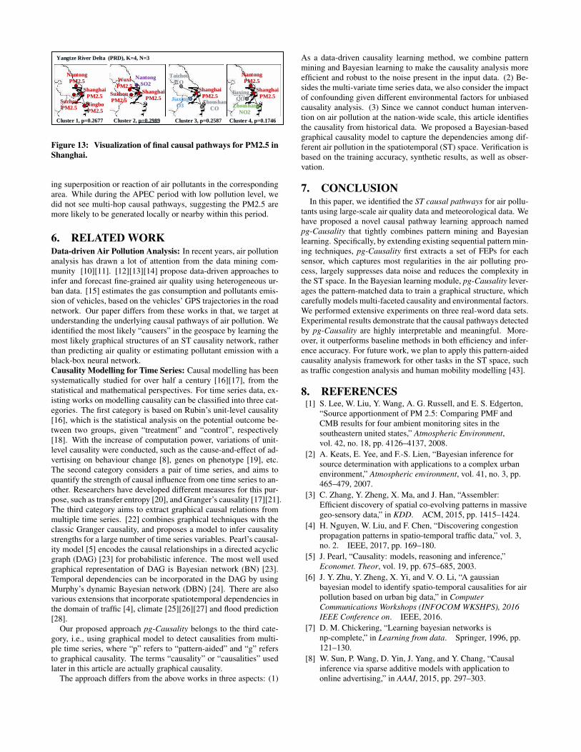
causal pathways for Beijing PM2.5 during Jan−Mar. We providethe probability for each causal pathway for each cluster, defined asthe proportion of labeled timestamps that belong to each cluster.As shown in Fig. 10(a), Cluster 3 takes a relatively higher pro-portion (28.52%) of time for Beijing PM2.5, indicating the causalpathway during Jan−Mar more probably come from southern sen-sors, i.e. Baoding and Cangzhou. Actions can be taken to controlthese pollutants in these cities. We then present the causal path-ways for PM2.5 in Shanghai, during Oct−Dec, which statisticallyhas the highest air pollution concentration. As shown in Fig. 13,for PM2.5 in Shanghai, the N = 3 neighborhood cities generallycome from the northwest and the southwest. Cluster 2 takes a rel-atively higher proportion (29.89%) of time for Shanghai PM2.5,suggesting the pollutants may be dispersed from PM2.5 in Suzhouand Wuxi, and SO2 in Nantong.2. Beijing during APEC period. Traditionally, causality is veri-fied via interventions in a causal system. For example, we can ver-ify the effect of a medicine by setting two groups of patients andonly giving medicine to the treatment group. However, it is impos-sible to conduct intervention for air pollutants in the real environ-ment. APEC period is a good opportunity to verify the causality,since the Chinese government shuttered factories in NC, and im-plemented traffic bans in and around Beijing [42]. Therefore, wecompare the causal pathways for PM2.5 in Beijing before and dur-ing the APEC period. To illustrate the propagation of pollutantsalong the causal pathway, we connect the one-hop pathway to 3-hop as shown in Fig. 14(a)(b). The connection originates from thetarget pollutant, i.e., Beijing PM2.5, and connect its causal pollu-tants at neighbor cities. Then for each new connected pollutant,we repeat the same procedure for the next hop. The connectionstops if in inference accuracy of one target pollutant based on itshistorical data is higher than based on the historical data of its ST“causers”, indicating the pollutant is more likely to be generatedlocally. Fig. 14(a) shows Beijing’s PM2.5 is likely to be caused byNO2 in Baoding (City 14), and PM10 in Cangzhou (City 18), dur-ing Jan − Mar. Further, for example, Cangzhou’s PM10 is mostlyinfluenced by PM10 in Dingzhou (City 15) and Binzhou (City 71),as well as PM2.5 in Dezhou (City 64). We list the information ofall 128 cities in Fig. 15, as well as their corresponding optimal Kand N for pollutant PM2.5 in Spring. Note that the causal path-ways forms “circles” in the southwestern cities to Beijing, which isidentical to the locations of the major plants in NC shown in Fig.14(c). However, we notice that the causal pathway cannot be con-nected into 3-hops during the APEC period, since each “causer”pollutant to Beijing PM2.5 (i.e. NO2 in Chengde and Zhangjiakou,and Tianjin) is more likely to be inferred by its own historical dataover its ST “causers” in this period. This may suggest the PM2.5in Beijing during the APEC period are mostly affected by pollu-tants locally and nearby. The 3-hop causal pathways learnt by threebaselines are quite similar, thus we only present the result learnedby CGBN, pg-Causality-p, pg-Causality-n, MWST, and MCMC inFig. 14(d-h). Our approach has better interpretability. It is notedthat without pattern mining module, the candidate “causers” forBeijing tend to be at irrelevant locations. While without integrat-ing confounders, the causal pathways tend to have too many pathsto be distinguished. We summarize the discovery for Beijing’s airpollution as follows.• Among all the cities within a region, a target pollutant can be

mainly affected by only several cities in the ST space. The locationsof most influential cities to a target pollutant demonstrate seasonalsimilarities.• The causal pathways for PM2.5 in Beijing may come in mul-

tiple hops that form “circle” in the southwest of Beijing, suggest-

Shanghai

PM2.5Shanghai

PM2.5

Shanghai

PM2.5

Nantong

PM2.5

Suzhou

PM2.5

Wuxi

PM2.5

Nantong

SO2

Taizhou

CO

Jiaxing

O3

Cluster 1, p=0.2677 Cluster 2, p=0.2989 Cluster 3, p=0.2587

Yangtze River Delta (PRD), K=4, N=3

Shanghai

PM2.5Jiaxing

CO

Zhoushan

NO2

Cluster 4, p=0.1746

Ningbo

PM2.5

Suzhou

PM2.5 Zhoushan

CO

Nantong

PM2.5

Figure 13: Visualization of final causal pathways for PM2.5 inShanghai.

ing superposition or reaction of air pollutants in the correspondingarea. While during the APEC period with low pollution level, wedid not see multi-hop causal pathways, suggesting the PM2.5 aremore likely to be generated locally or nearby within this period.

6. RELATED WORKData-driven Air Pollution Analysis: In recent years, air pollutionanalysis has drawn a lot of attention from the data mining com-munity [10][11]. [12][13][14] propose data-driven approaches toinfer and forecast fine-grained air quality using heterogeneous ur-ban data. [15] estimates the gas consumption and pollutants emis-sion of vehicles, based on the vehicles’ GPS trajectories in the roadnetwork. Our paper differs from these works in that, we target atunderstanding the underlying causal pathways of air pollution. Weidentified the most likely “causers” in the geospace by learning themost likely graphical structures of an ST causality network, ratherthan predicting air quality or estimating pollutant emission with ablack-box neural network.Causality Modelling for Time Series: Causal modelling has beensystematically studied for over half a century [16][17], from thestatistical and mathematical perspectives. For time series data, ex-isting works on modelling causality can be classified into three cat-egories. The first category is based on Rubin’s unit-level causality[16], which is the statistical analysis on the potential outcome be-tween two groups, given “treatment” and “control”, respectively[18]. With the increase of computation power, variations of unit-level causality were conducted, such as the cause-and-effect of ad-vertising on behaviour change [8], genes on phenotype [19], etc.The second category considers a pair of time series, and aims toquantify the strength of causal influence from one time series to an-other. Researchers have developed different measures for this pur-pose, such as transfer entropy [20], and Granger’s causality [17][21].The third category aims to extract graphical causal relations frommultiple time series. [22] combines graphical techniques with theclassic Granger causality, and proposes a model to infer causalitystrengths for a large number of time series variables. Pearl’s causal-ity model [5] encodes the causal relationships in a directed acyclicgraph (DAG) [23] for probabilistic inference. The most well usedgraphical representation of DAG is Bayesian network (BN) [23].Temporal dependencies can be incorporated in the DAG by usingMurphy’s dynamic Bayesian network (DBN) [24]. There are alsovarious extensions that incorporate spatiotemporal dependencies inthe domain of traffic [4], climate [25][26][27] and flood prediction[28].

Our proposed approach pg-Causality belongs to the third cate-gory, i.e., using graphical model to detect causalities from multi-ple time series, where “p” refers to “pattern-aided” and “g” refersto graphical causality. The terms “causality” or “causalities” usedlater in this article are actually graphical causality.

The approach differs from the above works in three aspects: (1)

As a data-driven causality learning method, we combine patternmining and Bayesian learning to make the causality analysis moreefficient and robust to the noise present in the input data. (2) Be-sides the multi-variate time series data, we also consider the impactof confounding given different environmental factors for unbiasedcausality analysis. (3) Since we cannot conduct human interven-tion on air pollution at the nation-wide scale, this article identifiesthe causality from historical data. We proposed a Bayesian-basedgraphical causality model to capture the dependencies among dif-ferent air pollution in the spatiotemporal (ST) space. Verification isbased on the training accuracy, synthetic results, as well as obser-vation.

7. CONCLUSIONIn this paper, we identified the ST causal pathways for air pollu-

tants using large-scale air quality data and meteorological data. Wehave proposed a novel causal pathway learning approach namedpg-Causality that tightly combines pattern mining and Bayesianlearning. Specifically, by extending existing sequential pattern min-ing techniques, pg-Causality first extracts a set of FEPs for eachsensor, which captures most regularities in the air polluting pro-cess, largely suppresses data noise and reduces the complexity inthe ST space. In the Bayesian learning module, pg-Causality lever-ages the pattern-matched data to train a graphical structure, whichcarefully models multi-faceted causality and environmental factors.We performed extensive experiments on three real-word data sets.Experimental results demonstrate that the causal pathways detectedby pg-Causality are highly interpretable and meaningful. More-over, it outperforms baseline methods in both efficiency and infer-ence accuracy. For future work, we plan to apply this pattern-aidedcausality analysis framework for other tasks in the ST space, suchas traffic congestion analysis and human mobility modelling [43].

8. REFERENCES[1] S. Lee, W. Liu, Y. Wang, A. G. Russell, and E. S. Edgerton,

“Source apportionment of PM 2.5: Comparing PMF andCMB results for four ambient monitoring sites in thesoutheastern united states,” Atmospheric Environment,vol. 42, no. 18, pp. 4126–4137, 2008.

[2] A. Keats, E. Yee, and F.-S. Lien, “Bayesian inference forsource determination with applications to a complex urbanenvironment,” Atmospheric environment, vol. 41, no. 3, pp.465–479, 2007.

[3] C. Zhang, Y. Zheng, X. Ma, and J. Han, “Assembler:Efficient discovery of spatial co-evolving patterns in massivegeo-sensory data,” in KDD. ACM, 2015, pp. 1415–1424.

[4] H. Nguyen, W. Liu, and F. Chen, “Discovering congestionpropagation patterns in spatio-temporal traffic data,” vol. 3,no. 2. IEEE, 2017, pp. 169–180.

[5] J. Pearl, “Causality: models, reasoning and inference,”Economet. Theor, vol. 19, pp. 675–685, 2003.

[6] J. Y. Zhu, Y. Zheng, X. Yi, and V. O. Li, “A gaussianbayesian model to identify spatio-temporal causalities for airpollution based on urban big data,” in ComputerCommunications Workshops (INFOCOM WKSHPS), 2016IEEE Conference on. IEEE, 2016.

[7] D. M. Chickering, “Learning bayesian networks isnp-complete,” in Learning from data. Springer, 1996, pp.121–130.

[8] W. Sun, P. Wang, D. Yin, J. Yang, and Y. Chang, “Causalinference via sparse additive models with application toonline advertising,” in AAAI, 2015, pp. 297–303.

Beijing

(c) Locations of major plants in the center

of North China

(a) Causal pathway for Beijing PM2.5,

pg-Causality, Jan-Mar

(e) Causal pathway for Beijing PM2.5,

pg-Causality-p, Jan-Mar

(f) Causal pathway for Beijing PM2.5,

pg-Causality-n, Jan-Mar

(g) Causal pathway for Beijing PM2.5,

MWST, Jan-Mar

(b) Causal pathway for Beijing PM2.5,

pg-Causality, APEC period

BeijingBeijing

BeijingBeijing Beijing

PM2.5

NO2NO2NO2NO2

PM2.5PM2.5PM2.5PM2.5

PM2.5PM2.5PM2.5PM2.5PM2.5PM2.5

PM2.5PM2.5PM2.5PM2.5 NO2

NO2

PM2.5PM2.5PM2.5PM2.5PM2.5PM2.5PM2.5

PM2.5PM2.5PM2.5

PM2.5

NO2NO2

NO2NO2NO2

NO2NO2

PM2.5PM2.5

PM2.5

SO2SO2SO2SO2

PM2.5PM2.5

PM2.5PM2.5

NO2NO2

NO2NO2NO2

PM2.5PM2.5PM2.5PM2.5PM2.5

PM2.5

SO2SO2SO2

PM2.5PM2.5

PM2.5

PM2.5

PM2.5

PM2.5

NO2

NO2SO2SO2SO2SO2SO2

PM2.5PM2.5PM2.5PM2.5

SO2SO2

NO2NO2

PM10PM10PM10PM10 PM2.5PM2.5

PM2.5

PM2.5

PM2.5 PM2.5

PM10

PM2.5

NO2

PM2.5

PM2.5

SO2

PM2.5

PM10

NO2

PM2.5

NO2

NO2PM2.5PM2.5

PM2.5

PM2.5

SO2

PM2.5

PM2.5

PM10

PM10PM2.5

PM2.5 PM2.5PM2.5

PM2.5

PM2.5

PM2.5PM2.5

PM2.5PM2.5PM2.5 SO2

NO2

NO2

PM10PM2.5

PM10PM2.5PM2.5

(h) Causal pathway for Beijing PM2.5,

K2+PS, Jan-Mar

(d) Causal pathway for Beijing PM2.5,

CGBN, Jan-Mar

BeijingPM2.5

NO2

PM10NO2

NO2

O3

O3

PM10

PM2.5

PM10

NO2

PM2.5 O3

O3

BeijingPM2.5

NO2

NO2

NO2

Figure 14: The causal pathways for Beijing PM2.5 before (a) and during APEC period (b), compared with the locations of majorplants in Hebei Province, China (c), and the causal pathways learned by baseline method CGBN (d), pg-Causality-p (e), pg-Causality-n (f), MWST (g), MCMC (h).

City No. City_Name Latitude Longitude K N Accuracy Region City No. City_Name Latitude Longitude K N Accuracy Region City No. City_Name Latitude Longitude K N Accuracy Region

1 Beijing 39.993 116.413 4 2 0.925 NC 44 Huludao 40.751 120.851 1 1 0.811 NC 87 Yancheng 33.391 120.157 1 1 0.891 YRD

2 Shanghai 31.184 121.456 5 0 0.938 YRD 45 Huhehaote 40.801 111.665 1 0 0.834 NC 88 Xuzhou 34.315 117.359 2 0 0.930 YRD

3 Shenzhen 22.635 114.121 1 0 0.954 PRD 46 Baotou 40.573 110.022 1 0 0.860 NC 89 Huaian 33.582 119.036 4 0 0.912 YRD

4 Ningbo 29.832 121.509 2 0 0.933 YRD 47 Wulanchabu 41.015 113.114 2 1 0.799 NC 90 Lianyungang 34.657 119.258 1 0 0.891 YRD

5 Tianjin 39.156 117.306 1 5 0.931 NC 48 Chifeng 42.210 119.008 1 0 0.869 NC 91 Changzhou 31.787 119.962 5 2 0.916 YRD

6 Guangzhou 23.159 113.377 4 0 0.957 PRD 49 Erduosi 39.813 110.002 6 0 0.786 NC 92 Taizhou 32.367 120.031 2 1 0.939 YRD

7 Hong Kong 22.343 114.163 4 0 0.948 PRD 50 Taiyuan 37.863 112.517 4 1 0.898 NC 93 Suqian 33.956 118.281 2 5 0.916 YRD

8 Shijiazhuang 38.045 114.588 4 3 0.921 NC 51 Datong 40.094 113.303 1 2 0.890 NC 94 Huangshi 30.216 115.055 1 0 0.954 YRD

9 Xinji 37.949 115.224 1 0 0.872 NC 52 Yangquan 37.861 113.566 2 5 0.931 NC 95 Hangzhou 30.076 119.893 3 1 0.936 YRD

10 Tangshan 39.720 118.311 1 4 0.908 NC 53 Jinzhong 37.696 112.734 6 1 0.910 NC 96 Huzhou 30.787 119.951 1 0 0.957 YRD

11 Qinhuangdao 39.955 119.367 6 1 0.887 NC 54 Changzhi 36.190 113.109 1 3 0.940 NC 97 Jiaxing 30.655 120.809 1 0 0.907 YRD

12 Handan 36.568 114.659 2 1 0.937 NC 55 Jincheng 35.498 112.849 4 2 0.838 NC 98 Shaoxing 29.869 120.613 1 5 0.890 YRD

13 Xingtai 37.185 114.879 1 0 0.921 NC 56 Linfen 36.078 111.514 1 0 0.938 NC 99 Taizhou 28.683 121.197 1 0 0.910 YRD

14 Baoding 38.933 115.474 5 0 0.926 NC 57 Yuncheng 35.041 111.015 1 0 0.903 NC 100 Wenzhou 28.061 120.753 1 1 0.916 YRD

15 Dingzhou 38.522 114.997 1 1 0.855 NC 58 Shuozhou 39.344 112.431 3 0 0.790 NC 101 Lishui 28.349 119.704 1 5 0.896 YRD

16 Zhangjiakou 40.787 114.925 2 2 0.846 NC 59 Yizhou 38.443 112.726 1 3 0.859 NC 102 Jinhua 29.160 119.902 5 0 0.896 YRD

17 Chengde 40.974 117.833 2 0 0.861 NC 60 Lvliang 37.522 111.136 1 0 0.863 NC 103 Quzhou 28.942 118.777 2 0 0.901 YRD

18 Cangzhou 38.224 116.688 2 0 0.921 NC 61 Jinan 36.644 117.030 2 5 0.922 NC 104 Zhoushan 30.034 122.238 1 1 0.894 YRD

19 Langfang 39.444 116.694 1 0 0.893 NC 62 Qingdao 36.123 120.384 1 4 0.922 NC 105 Hefei 31.848 117.248 7 0 0.910 YRD

20 Hengshui 37.809 115.800 1 5 0.917 NC 63 Zibo 36.744 118.005 1 0 0.921 NC 106 Bengbu 32.929 117.357 1 5 0.892 YRD

21 Dongguan 23.024 113.762 2 1 0.932 PRD 64 Dezhou 37.459 116.328 1 3 0.886 NC 107 Wuhu 31.366 118.375 1 1 0.896 YRD

22 Foshan 22.988 113.063 2 1 0.933 PRD 65 Yantai 37.511 121.336 1 0 0.902 NC 108 Whuainan 32.655 116.874 6 3 0.880 YRD

23 Heyuan 23.746 114.687 1 0 -- PRD 66 Weifang 36.709 119.124 2 1 0.898 NC 109 Maanshan 31.697 118.525 1 1 0.934 YRD

24 Huizhou 23.012 114.368 1 0 0.935 PRD 67 Jining 35.409 116.622 2 0 0.935 NC 110 Anqing 30.547 117.031 1 0 0.914 YRD

25 Jiangmen 22.516 112.912 5 0 0.894 PRD 68 Taian 36.180 117.122 1 0 0.899 NC 111 Suzhou 33.639 116.971 1 1 0.879 YRD

26 Jieyang 22.593 113.082 4 0 0.861 PRD 69 Linyi 35.053 118.329 1 0 0.919 NC 112 Fuyang 32.881 115.831 1 0 0.883 YRD

27 Qingyuan 23.677 113.042 7 0 0.917 PRD 70 Heze 35.248 115.468 2 0 0.913 NC 113 Bozhou 33.848 115.795 1 1 0.898 YRD

28 Shanwei 22.783 115.371 1 1 0.906 PRD 71 Binzhou 37.374 117.975 2 2 0.882 NC 114 Huangshan 29.903 118.255 3 0 0.804 YRD

29 Shaoguan 24.772 113.593 3 0 0.930 PRD 72 Dongying 37.488 118.614 1 1 0.896 NC 115 Chuzhou 32.300 118.317 1 0 0.883 YRD

30 Yunfu 22.937 112.043 1 0 0.925 PRD 73 Weihai 37.475 122.092 7 1 0.903 NC 116 Huaibei 33.940 116.797 1 0 0.895 YRD

31 Zhaoqing 23.091 112.484 3 1 0.898 PRD 74 Zaozhuang 34.815 117.481 1 1 0.921 NC 117 Tongling 30.936 117.820 1 0 0.889 YRD

32 Zhongshan 22.516 113.392 1 0 0.943 PRD 75 Rizhao 35.393 119.501 1 0 0.888 NC 118 Xuancheng 30.954 118.738 1 0 0.888 YRD

33 Zhuhai 22.285 113.501 1 0 0.922 PRD 76 Laiwu 36.209 117.726 1 1 0.932 NC 119 Liuan 31.762 116.515 3 5 0.907 YRD

34 Nanjing 31.985 118.816 2 2 0.917 YRD 77 Liaocheng 36.457 115.982 2 2 0.922 NC 120 Chizhou 30.652 117.483 1 0 0.831 YRD

35 Suzhou 31.438 120.716 5 0 0.938 YRD 78 Anyang 36.096 114.392 1 0 0.864 NC 121 Nanchang 28.690 115.879 1 5 0.883 YRD

36 Wuxi 31.616 120.209 1 2 0.930 YRD 79 Xinxiang 35.293 113.923 5 3 0.890 NC 122 Jiujiang 29.672 116.002 1 1 0.944 YRD

37 Dalian 38.950 121.628 3 0 0.900 NC 80 Shangqiu 34.417 115.655 1 0 0.883 YRD 123 Shangrao 28.449 117.958 6 0 0.951 YRD

38 Anshan 41.096 122.968 2 2 0.867 NC 81 Jiaozuo 35.223 113.235 1 4 0.917 NC 124 Fuzhou 28.040 116.291 7 0 0.942 YRD

39 Jinzhou 41.059 121.128 1 0 0.804 NC 82 Hebi 35.744 114.301 6 0 0.932 NC 125 Jingdezhen 29.304 117.224 1 0 0.946 YRD

40 Yingkou 40.676 122.222 4 0 0.839 NC 83 Puyang 35.772 115.053 1 3 0.909 NC 126 Yingtan 28.209 117.013 1 0 0.910 YRD

41 Fuxin 42.042 121.685 1 0 0.837 NC 84 Zhenjiang 32.108 119.477 3 2 0.920 YRD 127 Wuzhou 23.462 111.276 2 0 0.941 PRD

42 Chaoyang 41.692 120.461 1 0 0.730 NC 85 Nantong 31.990 120.879 1 2 0.903 YRD 128 Hezhou 24.413 111.544 1 0 0.903 PRD

43 Panjin 41.151 122.032 2 2 0.847 NC 86 Yangzhou 32.537 119.397 5 0 0.938 YRD

Figure 15: Optimal K and N for 128 cities, in Region NC, YRD and PRD, for PM2.5 during Jan −Mar.

[9] C. Zhang, J. Han, L. Shou, J. Lu, and T. La Porta, “Splitter:Mining fine-grained sequential patterns in semantictrajectories,” Proceedings of the VLDB Endowment, vol. 7,no. 9, pp. 769–780, 2014.

[10] Y. Zheng, L. Capra, O. Wolfson, and H. Yang, “Urbancomputing: concepts, methodologies, and applications,”ACM Transactions on Intelligent Systems and Technology(TIST), vol. 5, no. 3, p. 38, 2014.

[11] Y. Zheng, “Methodologies for cross-domain data fusion: Anoverview,” IEEE transactions on big data, vol. 1, no. 1, pp.16–34, 2015.

[12] Y. Zheng, F. Liu, and H.-P. Hsieh, “U-air: When urban airquality inference meets big data,” in KDD. ACM, 2013, pp.1436–1444.

[13] Y. Zheng, X. Yi, M. Li, R. Li, Z. Shan, E. Chang, and T. Li,“Forecasting fine-grained air quality based on big data,” in

KDD, 2015.[14] H.-P. Hsieh, S.-D. Lin, and Y. Zheng, “Inferring air quality

for station location recommendation based on urban bigdata,” in Proceedings of the 21th ACM SIGKDDInternational Conference on Knowledge Discovery and DataMining. ACM, 2015, pp. 437–446.

[15] J. Shang, Y. Zheng, W. Tong, E. Chang, and Y. Yu, “Inferringgas consumption and pollution emission of vehiclesthroughout a city,” in KDD, 2014.

[16] D. B. Rubin, “Estimating causal effects of treatments inrandomized and nonrandomized studies.” Journal ofeducational Psychology, vol. 66, no. 5, p. 688, 1974.

[17] C. W. Granger, “Investigating causal relations byeconometric models and cross-spectral methods,”Econometrica: Journal of the Econometric Society, pp.424–438, 1969.

[18] P. R. Rosenbaum and D. B. Rubin, “The central role of thepropensity score in observational studies for causal effects,”Biometrika, pp. 41–55, 1983.

[19] D. S. Wald, M. Law, and J. K. Morris, “Homocysteine andcardiovascular disease: evidence on causality from ameta-analysis,” Bmj, vol. 325, no. 7374, p. 1202, 2002.

[20] L. Barnett, A. B. Barrett, and A. K. Seth, “Granger causalityand transfer entropy are equivalent for gaussian variables,”Physical Review Letters, 2009.

[21] K. Hlavácková-Schindler, M. Palus, M. Vejmelka, andJ. Bhattacharya, “Causality detection based oninformation-theoretic approaches in time series analysis,”Physics Reports, vol. 441, no. 1, pp. 1–46, 2007.

[22] A. Arnold, Y. Liu, and N. Abe, “Temporal causal modelingwith graphical granger methods,” in KDD. ACM, 2007, pp.66–75.

[23] D. Heckerman, D. Geiger, and D. M. Chickering, “Learningbayesian networks: The combination of knowledge andstatistical data,” Machine Learning, vol. 20, no. 3, pp.197–243, 1995.

[24] K. P. Murphy, “Dynamic Bayesian Networks:Representation, Inference and Learning,” Ph.D. dissertation,University of California, Berkeley, 2002.

[25] I. Ebert-Uphoff and Y. Deng, “Causal discovery fromspatio-temporal data with applications to climate science,” inMachine Learning and Applications (ICMLA), 2014 13thInternational Conference on. IEEE, 2014, pp. 606–613.

[26] J. Runge, J. Heitzig, V. Petoukhov, and J. Kurths, “Escapingthe curse of dimensionality in estimating multivariatetransfer entropy,” Physical review letters, vol. 108, no. 25, p.258701, 2012.

[27] A. C. Lozano, H. Li, A. Niculescu-Mizil, Y. Liu, C. Perlich,J. Hosking, and N. Abe, “Spatial-temporal causal modelingfor climate change attribution,” in Proceedings of the 15thACM SIGKDD international conference on Knowledgediscovery and data mining. ACM, 2009, pp. 587–596.

[28] P. Jangyodsuk, D.-J. Seo, R. Elmasri, and J. Gao, “Floodprediction and mining influential spatial features on futureflood with causal discovery,” in Data Mining Workshop(ICDMW), 2015 IEEE International Conference on. IEEE,2015, pp. 1462–1469.

[29] J. Pel, J. Han, B. Mortazavi-Asl, H. Pinto, Q. Chen,U. Dayal, and M. Hsu, “Prefixspan: Mining sequentialpatterns by prefix-projected growth,” in Proc. 17th IEEEInternational Conference on Data Engineering (ICDE).

Heidelberg, Germany, 2001, pp. 215–224.[30] J. Lin, E. Keogh, S. Lonardi, and B. Chiu, “A symbolic

representation of time series, with implications for streamingalgorithms,” in SIGMOD, 2003.

[31] P. W. Holland, “Statistics and causal inference,” Journal ofthe American statistical Association, vol. 81, no. 396, pp.945–960, 1986.

[32] M. A. Gómez, P. M. Villegasa, H. Navarrob, and R. Susia,“Dealing with uncertainty in gaussian bayesian networksfrom a regression perspective,” on Probabilistic GraphicalModels, p. 145, 2010.

[33] R. D’Agostino and E. S. Pearson, “Tests for departure fromnormality. empirical results for the distributions of b2 andb1,” Biometrika, vol. 60, no. 3, pp. 613–622, 1973.

[34] J. Y. Zhu, C. Sun, and V. O. Li, “Granger-causality-based airquality estimation with spatio-temporal (st) heterogeneousbig data,” in Computer Communications Workshops(INFOCOM WKSHPS), 2015 IEEE Conference on. IEEE,2015, pp. 612–617.

[35] I. Flesch and P. J. Lucas, “Markov equivalence in bayesiannetworks,” in Advances in Probabilistic Graphical Models.Springer, 2007, pp. 3–38.

[36] K. Murphy et al., “The bayes net toolbox for matlab,”Computing science and statistics, vol. 33, no. 2, pp.1024–1034, 2001.

[37] C. Chow and C. Liu, “Approximating discrete probabilitydistributions with dependence trees,” Information Theory,IEEE Transactions on, 1968.

[38] G. Rebane and J. Pearl, “The recovery of causal poly-treesfrom statistical data,” pp. 222–228, 1987.

[39] J. L. Beck and S.-K. Au, “Bayesian updating of structuralmodels and reliability using markov chain monte carlosimulation,” Journal of Engineering Mechanics, vol. 128,no. 4, pp. 380–391, 2002.

[40] G. F. Cooper and E. Herskovits, “A bayesian method for theinduction of probabilistic networks from data,” MachineLearning, vol. 9, no. 4, pp. 309–347, 1992.

[41] R. M. Lewis and V. Torczon, “A globally convergentaugmented lagrangian pattern search algorithm foroptimization with general constraints and simple bounds,”SIAM Journal on Optimization, vol. 12, no. 4, pp.1075–1089, 2002.

[42] K. Huang, X. Zhang, and Y. Lin, “The “apec blue”phenomenon: Regional emission control effects observedfrom space,” Atmospheric Research, vol. 164, pp. 65–75,2015.

[43] C. Zhang, K. Zhang, Q. Yuan, L. Zhang, T. Hanratty, andJ. Han, “Gmove: Group-level mobility modeling usinggeo-tagged social media,” in KDD, 2016, pp. 1305–1314.