285
| Date post: | 08-Nov-2014 |
| Category: |
Documents |
| Upload: | adrian-scurtu |
| View: | 69 times |
| Download: | 1 times |
Introduction to Dusty Plasma Physics
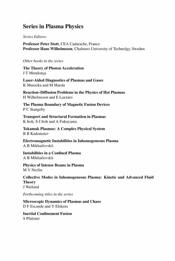
Series in Plasma Physics
Series Editors:
Professor Peter Stott, CEA Cadarache, FranceProfessor Hans Wilhelmsson, Chalmers University of Technolgy, Sweden
Other books in the series
The Theory of Photon AccelerationJ T Mendonca
Laser-Aided Diagnostics of Plasmas and GasesK Muraoka and M Maeda
Reaction–Diffusion Problems in the Physics of Hot PlasmasH Wilhelmsson and E Lazzaro
The Plasma Boundary of Magnetic Fusion DevicesP C Stangeby
Transport and Structural Formation in PlasmasK Itoh, S-I Itoh and A Fukuyama
Tokamak Plasmas: A Complex Physical SystemB B Kadomstev
Electromagnetic Instabilities in Inhomogeneous PlasmaA B Mikhailovskii
Instabilities in a Confined PlasmaA B Mikhailovskii
Physics of Intense Beams in PlasmaM V Nezlin
Collective Modes in Inhomogeneous Plasma: Kinetic and Advanced FluidTheoryJ Weiland
Forthcoming titles in the series
Microscopic Dynamics of Plasmas and ChaosD F Escande and Y Elskens
Inertial Confinement FusionS Pfalzner

Series in Plasma Physics
Introduction to Dusty PlasmaPhysics
P K Shukla
Ruhr-Universitat Bochum, Germany and UmeaUniversity, Sweden
A A Mamun
Jahangrinagar University, Dhaka, Bangladesh
Institute of Physics PublishingBristol and Philadelphia

c© IOP Publishing Ltd 2002
All rights reserved. No part of this publication may be reproduced, storedin a retrieval system or transmitted in any form or by any means, electronic,mechanical, photocopying, recording or otherwise, without the prior permissionof the publisher. Multiple copying is permitted in accordance with the termsof licences issued by the Copyright Licensing Agency under the terms of itsagreement with the Committee of Vice-Chancellors and Principals.
British Library Cataloguing-in-Publication Data
A catalogue record for this book is available from the British Library.
ISBN 0 7503 0653 X
Library of Congress Cataloging-in-Publication Data are available
Commissioning Editor: John NavasProduction Editor: Simon LaurensonProduction Control: Sarah PlentyCover Design: Victoria Le BillonMarketing Executive: Laura Serratrice
Published by Institute of Physics Publishing, wholly owned by The Institute ofPhysics, London
Institute of Physics Publishing, Dirac House, Temple Back, Bristol BS1 6BE, UK
US Office: Institute of Physics Publishing, The Public Ledger Building, Suite1035, 150 South Independence Mall West, Philadelphia, PA 19106, USA
Typeset in LATEX 2ε by Text 2 Text, Torquay, DevonPrinted in the UK by MPG Books Ltd, Bodmin, Cornwall
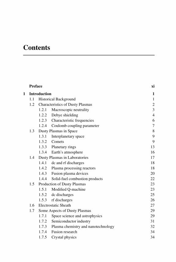
Contents
Preface xi
1 Introduction 11.1 Historical Background 11.2 Characteristics of Dusty Plasmas 2
1.2.1 Macroscopic neutrality 31.2.2 Debye shielding 41.2.3 Characteristic frequencies 61.2.4 Coulomb coupling parameter 7
1.3 Dusty Plasmas in Space 81.3.1 Interplanetary space 91.3.2 Comets 91.3.3 Planetary rings 131.3.4 Earth’s atmosphere 16
1.4 Dusty Plasmas in Laboratories 171.4.1 dc and rf discharges 181.4.2 Plasma processing reactors 181.4.3 Fusion plasma devices 201.4.4 Solid-fuel combustion products 22
1.5 Production of Dusty Plasmas 231.5.1 Modified Q-machine 231.5.2 dc discharges 251.5.3 rf discharges 26
1.6 Electrostatic Sheath 271.7 Some Aspects of Dusty Plasmas 29
1.7.1 Space science and astrophysics 291.7.2 Semiconductor industry 311.7.3 Plasma chemistry and nanotechnology 321.7.4 Fusion research 341.7.5 Crystal physics 34
vi Contents
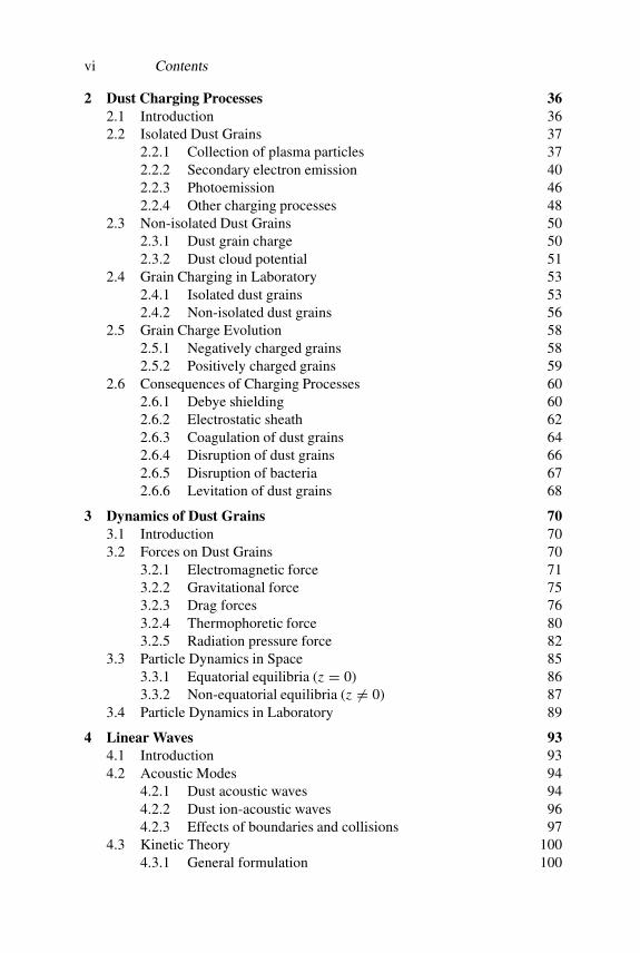
2 Dust Charging Processes 362.1 Introduction 362.2 Isolated Dust Grains 37
2.2.1 Collection of plasma particles 372.2.2 Secondary electron emission 402.2.3 Photoemission 462.2.4 Other charging processes 48
2.3 Non-isolated Dust Grains 502.3.1 Dust grain charge 502.3.2 Dust cloud potential 51
2.4 Grain Charging in Laboratory 532.4.1 Isolated dust grains 532.4.2 Non-isolated dust grains 56
2.5 Grain Charge Evolution 582.5.1 Negatively charged grains 582.5.2 Positively charged grains 59
2.6 Consequences of Charging Processes 602.6.1 Debye shielding 602.6.2 Electrostatic sheath 622.6.3 Coagulation of dust grains 642.6.4 Disruption of dust grains 662.6.5 Disruption of bacteria 672.6.6 Levitation of dust grains 68
3 Dynamics of Dust Grains 703.1 Introduction 703.2 Forces on Dust Grains 70
3.2.1 Electromagnetic force 713.2.2 Gravitational force 753.2.3 Drag forces 763.2.4 Thermophoretic force 803.2.5 Radiation pressure force 82
3.3 Particle Dynamics in Space 853.3.1 Equatorial equilibria (z = 0) 863.3.2 Non-equatorial equilibria (z �= 0) 87
3.4 Particle Dynamics in Laboratory 89
4 Linear Waves 934.1 Introduction 934.2 Acoustic Modes 94
4.2.1 Dust acoustic waves 944.2.2 Dust ion-acoustic waves 964.2.3 Effects of boundaries and collisions 97
4.3 Kinetic Theory 1004.3.1 General formulation 100

Contents vii
4.3.2 Results without Landau damping 1044.3.3 Landau damping rates 1064.3.4 Role of dust size distributions 107
4.4 Other Effects 1084.4.1 Thin dust layers 1084.4.2 Dust correlations 110
4.5 Dust Lattice Waves 1134.5.1 Longitudinal DL waves 1134.5.2 An improved model 114
4.6 Waves in Uniform Magnetoplasmas 1174.6.1 Electrostatic waves 1174.6.2 Electromagnetic waves 120
4.7 Waves in Non-uniform Magnetoplasmas 1234.7.1 Electrostatic waves 1244.7.2 Electromagnetic waves 126
4.8 Experimental Observations 1324.8.1 Dust acoustic waves 1324.8.2 Dust ion-acoustic waves 1344.8.3 Dust lattice waves 135
5 Instabilities 1385.1 Introduction 1385.2 Streaming Instabilities 139
5.2.1 Unmagnetized plasmas 1395.2.2 Magnetized plasmas 1415.2.3 Boundary effects 145
5.3 Ion Drag Force Induced Instabilities 1475.3.1 DIA waves 1495.3.2 DA waves 151
5.4 Dust Charge Gradient Induced Instabilities 1515.4.1 Equilibrium properties 1515.4.2 DA waves 1535.4.3 Transverse DL waves 155
5.5 Drift Wave Instabilities 1565.5.1 Universal instability 1565.5.2 Velocity shear instability 1585.5.3 Self-gravitational instability 159
5.6 Parametric Instabilities 1615.6.1 Modulational interactions 1615.6.2 Nonlinear particle oscillations 164
5.7 Laboratory Studies 1665.7.1 DA wave instability 1665.7.2 DIA wave instability 1665.7.3 EIC instability 168

viii Contents
6 Elongated Dust Grains 1706.1 Introduction 1706.2 Dust Charge and Current Densities 1716.3 Grain Kinetic Equation 1746.4 Dielectric Permittivity 175
6.4.1 Unmagnetized dusty plasmas 1766.4.2 Magnetized dusty plasmas 177
6.5 Dispersion Properties of the Waves 1796.5.1 Unmagnetized dusty plasmas 1806.5.2 Cold magnetized dusty plasmas 1826.5.3 Warm magnetized dusty plasmas 1866.5.4 Scattering cross section 188
6.6 Grain Vibration and Rotation 1896.6.1 Bouncing motion 1906.6.2 Vibrational motion 1906.6.3 Rotational and vibrational motions 192
7 Nonlinear Structures 1957.1 Introduction 1957.2 Solitary Waves 196
7.2.1 Small-amplitude DAS waves 1977.2.2 Arbitrary-amplitude DAS waves 1987.2.3 Effect of the dust fluid temperature 2007.2.4 Effect of the trapped ion distribution 2047.2.5 Effect of dust charge fluctuations 2077.2.6 Cylindrical and spherical DAS waves 2087.2.7 Double layers 2107.2.8 Dust lattice solitary waves 212
7.3 Shock Waves 2137.3.1 DA shock waves 2137.3.2 DIA shock waves 2147.3.3 Solutions of the KdV–Burgers equation 2157.3.4 Experimental observations of DIA shock waves 217
7.4 Envelope Solitons 2187.5 Vortices 221
7.5.1 Electrostatic vortices 2217.5.2 Electromagnetic vortices 224
8 Dust Crystals 2288.1 Preamble 2288.2 Properties of Plasma Crystals 2318.3 Potential of a Test Charge 2338.4 Attractive Forces 235
8.4.1 Electrostatic energy between dressed grains 2358.4.2 Wake potentials 236

Contents ix
8.4.3 Dipole–dipole interactions 2418.4.4 Shadowing force 2438.4.5 Experimental verification 245
8.5 Formation of Dust Crystals 2478.5.1 Thomas et al’s experiment 2478.5.2 Chu et al’s experiments 2488.5.3 Molotkov et al ’s experiment 2498.5.4 Phase transitions 251
8.6 Mach Cones 2538.7 Particle Dynamics: Microgravity Experiment 255
References 258
Index 266

Preface
This book presents an up-to-date account of collective processes in dusty plasmas.This is a new frontier in applied physics and modern technology. A dustyplasma is a complex system because of the variation of the dust grain charge,mass and size with space and time. It exhibits new and unusual behaviour, andprovides a possibility for modified or entirely new collective modes of oscillation,instabilities as well as coherent nonlinear structures. A particularly interestingaspect of a dusty plasma is that it can be strongly coupled, i.e. the interactionpotential energy between the dust grains can exceed their kinetic energy. As aresult, grain–grain correlations become important; for strong enough coupling,the dust grains can condense into a dusty plasma crystal configuration. It turnsout that the dynamics of dust particles produces phenomena on such a long timescale that they can even be seen with the naked eye.
This book is designed for students and scientists who possess a rudimentaryworking knowledge of wave motions in plasmas and fluids at the graduate level.It can be used for learning and teaching the essentials of dusty plasma physics andits applications to low-temperature laboratory and space environments.
Since the early 1990s there has been a great deal of interest in studying thephysics of dusty plasmas which has now become a new discipline in plasmascience. A large number of dusty plasma papers has appeared within the tenyears following the discovery of dust acoustic waves and dusty plasma crystals.Several conference proceedings have summarized the progress that has beenmade in dusty plasma research. However, the existing materials on collectiveprocesses in dusty plasmas are scattered, and there is a need for their unification.It is, therefore, timely to present an up-to-date, comprehensive and coherentdescription of dusty plasma physics in the form of an introductory book that,we hope, should be useful to readers who wish to learn and teach its essentialsand to familiarize themselves with the progress that has recently been made. Thisis the objective of the present book.
This book has grown out of the research work on topics on which theauthors have spent a considerable amount of time and thought. We have dealtwith the basic properties of dusty plasmas, the charging of dust grains and theirdynamics under the action of numerous forces, as well as various aspects ofcollective interactions including waves, linear and nonlinear instabilities, coherent
xi
xii Preface
nonlinear structures, new attractive forces, dust crystals, etc. The book isdivided into eight chapters covering the above-mentioned topics which have wide-ranging applications to laboratory and space dusty plasmas. CGS units are usedthroughout the book. The references included here are somewhat selective anddesigned to be representative of original ideas set forth on a particular theme.
The book is organized as follows. In chapter 1, we start with a rudimentaryintroduction to dusty plasma physics and point out how this differs from thatof the usual electron–ion plasma. Conditions for defining weakly and stronglycorrelated dusty plasmas are illustrated in terms of the Coulomb couplingparameter. The dust grain charging processes, which are amongst the mainingredients of dusty plasma physics, are described in chapter 2. Numerous forcesand dust grain dynamics are examined in chapter 3.
Chapter 4 deals with various types of waves in both unmagnetized andmagnetized dusty plasmas. Here, we have focused on low-frequency dust acoustic(DA), dust ion-acoustic (DIA) and dust lattice (DL) waves in an unmagnetizedplasma, while a great variety of waves appears when an external magnetic field isapplied to a uniform and non-uniform dusty plasma. The dust charge fluctuationsprovide a novel damping mechanism for the DA and DIA waves. The effects ofthe plasma boundaries and the dust–neutral as well as the dust–dust interactionson the propagation of the DA and DIA waves are also examined. When thespacing between the dust grains is of the order of the dusty plasma Debye radius,the dust grains interact with each other via the Debye–Huckel repulsive force.In such a situation, there arise DL waves due to lattice vibrations. Theoreticallypredicted dispersion properties of DA, DIA and DL waves are now experimentallyverified. The presence of both a magnetic field and plasma non-uniformitiesintroduces new types of dusty plasma waves, in addition to modifying the existingion-cyclotron and Alfven wave dispersion properties.
Chapter 5 presents various instabilities that drive low-frequency waves atnon-thermal levels in dusty plasmas. In addition to discussing the well knowninstabilities in infinite and bounded systems, we also present studies of some newinstabilities which involve ionization, the ion drag force, the dust charge gradient,the self-gravitation of dust grains, etc. Furthermore, we have also consideredseveral examples of parametric instabilities in weakly and strongly coupled dustyplasmas.
Chapter 6 is concerned with the electrodynamics and dispersion propertiesof a dusty plasma containing elongated and rotating dust grains that are of finitesize. Expressions for the dust charge and dust current densities are developed byincluding the dust dipole moment and the dust grain rotation. The dust rotationalenergy can excite different wave modes. Finally, studies of the dust grain vibrationand rotation in the presence of electromagnetic fields are carried out.
Chapter 7 is devoted to coherent nonlinear structures in dusty plasmas.We consider DA and DIA solitons and shocks as well as double layers in anunmagnetized dusty plasma. The coherent nonlinear structures produced by non-Maxwellian trapped particle distributions are also presented. Furthermore, we

Preface xiii
discuss the topic of self-organization in the form of coherent vortices. The focusis then on the stationary solutions of the nonlinear equations that govern thedynamics of low-frequency electrostatic and electromagnetic dispersive waves ina non-uniform dusty magnetoplasma.
Chapter 8 deals with the formation of dust crystals and the associatedattractive forces. The latter can come from overlapping Debye spheres, ionfocusing and wakefields, dipole–dipole interactions, and shadowing effects. Alsopresented are experimental demonstrations of the dust crystal formation and phasetransitions in strongly coupled radio-frequency and glow discharges. Some resultsfor the particulate dynamics under microgravity conditions are included as well.Finally, we have discussed the formation of multiple Mach cones in a two-dimensional dusty plasma crystal. Evidently, the dusty plasma crystal opens anew area for the study of strongly coupled Coulomb systems. A detailed study ofCoulomb crystal structures is expected to advance the research and growth of anatomic crystal, as well as the analysis of forces acting on them, which is usefulfor the development of the control of dust in processing plasmas.
We are grateful to Professor Lennart Stenflo and Dr Horst Fichtner whokindly read the entire book and offered valuable suggestions for improvements.We have greatly benefited from many enlightening discussions with a numberof physicists including Professors Robert Bingham, Alan Cairns, John Dawson,Umberto de Angelis, Ove Havnes, Asoka Mendis, Frank Melandsø, Jose TitoMendonca, Gregor Morfill, Mitsuhiro Nambu, Nagesha Rao, David Resendes,Marlene Rosenberg, Mohammed Salimullah, Lennart Stenflo, David Tskhakaya,Ram Varma and Frank Verheest. A A Mamun thanks the Alexander vonHumboldt Foundation for financial support. This work could not have beencompleted without the substantial help and constant encouragement of our wivesRanjana Shukla and Khurshida Khayer Mamun.
P K Shukla and A A MamunMay 2001


Chapter 1
Introduction
1.1 Historical Background
About 70 years ago Tonks and Langmuir (1929) first coined the term ‘plasma’to describe the inner region (remote from the boundaries) of a glowing ionizedgas produced by means of an electric discharge in a tube. The term plasmarepresents a macroscopically neutral gas containing many interacting chargedparticles (electrons and ions) and neutrals. It is likely that 99% of the matter in ouruniverse (in which the dust is one of the omnipresent ingredients) is in the formof a plasma. Thus, in most cases a plasma coexists with the dust particulates.These particulates may be as large as a micron. They are not neutral, but arecharged either negatively or positively depending on their surrounding plasmaenvironments. An admixture of such charged dust or macro-particles, electrons,ions and neutrals forms a ‘dusty plasma’.
The history of dusty plasmas is quite old (Mendis 1997). A bright cometobserved by our distant ancestors is an excellent cosmic laboratory for the studyof dust–plasma interactions and their physical and dynamical consequences. Theother manifestations of dust-laden plasmas observed by the ancients would havebeen the zodiacal light (a triangular glow rising above the horizon shortly afterSunset or before Sunrise), the Orion Nebula (faintly visible to the naked eye as astar in the sword of the hunter in the Orion constellation), the noctilucent clouds(observed at the Earth’s polar summer mesopause), etc. An almost incrediblenumber of images of astrophysical objects (e.g. the Eagle Nebula, planetary rings,etc) have recently been obtained by the Hubble Space Telescope and spacecraft.
Observations of dust-laden plasmas in the terrestrial laboratory were alsoavailable in the remote past. The fact that an ordinary flame is considered as aplasma may come as a surprise due to the high-level of collisionality within it.However, strictly it is not: what makes it close to being a plasma is the presenceof minute (∼100 A) particles of unburnt carbon (soot). While the yellow lightemitted by typical hydrocarbon flames (namely candles) is due to incandescenceof these small particulates heated to well over 1000 ◦C, the thermionic emission
1
2 Introduction
of electrons from them elevates the degree of ionization within the flame severalorders of magnitude above what is given by the Saha equation for air at thattemperature. Thus, it is amazing that the ancients thought of fire as a fourth stateof matter (other than earth, water and air), while we have given this designationto a plasma only about 70 years ago.
There are a number of more recent examples of dust-laden plasmas inthe terrestrial environments. These are rocket and space shuttle exhausts,thermonuclear fireballs, processing plasmas used in device fabrications (e.g.microchips for computers), dusty plasmas created in laboratories for studyingbasic collective processes, plasma crystals, etc.
1.2 Characteristics of Dusty Plasmas
A dusty plasma is loosely defined as a normal electron–ion plasma with anadditional charged component of micron- or submicron-sized particulates. Thisextra component of macro-particles increases the complexity of the systemeven further. This is why a dusty plasma is also referred to as a ‘complexplasma’. Dusty plasmas are low-temperature fully or partially ionized electricallyconducting gases whose constituents are electrons, ions, charged dust grainsand neutral atoms. Dust grains are massive (billions times heavier than theprotons) and their sizes range from nanometres to millimetres. Dust grains maybe metallic, conducting, or made of ice particulates. The size and shape of dustgrains will be different, unless they are man-made. However, when viewed fromafar, they can be considered as point charges.
A plasma with dust particles or grains can be termed as either ‘dust ina plasma’ or ‘a dusty plasma’ depending on the ordering of a number ofcharacteristic lengths. These are the dust grain radius (rd), the average intergraindistance (a), the plasma Debye radius (λD) and the dimension of the dusty plasma.The situation rd � λD < a (in which charged dust particles are consideredas a collection of isolated screened grains) corresponds to ‘dust in a plasma’,while the situation rd � a < λD (in which charged dust particles participate inthe collective behaviour) corresponds to ‘a dusty plasma’. When we considera plasma with isolated dust grains (a � λD), we should take into accountthe local plasma inhomogeneities. On the other hand, when we consider theopposite situation (a � λD), we should treat dust grains as massive chargedparticles similar to multiply charged negative or positive ions. However, instudies of collective dusty plasma behaviour, we should also take into accountthe dust particle charging processes (which we describe in chapter 2). The basicdifferences between a dusty plasma and an electron–ion (or multi-ion) plasmaare pointed out in table 1.1. The table shows that there exists some distributionfor the dust grain charge–mass ratio (qd/md). The interaction between dustgrains is screened by the background electrons and ions. The presence ofcharged dust grains does not only modify the existing low-frequency waves

Characteristics of Dusty Plasmas 3
Table 1.1. The basic differences between electron–ion and dusty plasmas.
Characteristics Electron–ion plasma Dusty plasma
Quasi-neutrality condition ne0 = Zini0 Zdnd0 + ne0 = Zini0Massive particle charge qi = Zie |qd| = Zde � qiCharge dynamics qi = constant ∂qd/∂t = net currentMassive particle mass mi md � miPlasma frequency ωpi ωpd � ωpiDebye radius λDe λDi � λDeParticle size uniform dust size distributionE × B0 particle drift ion drift at low B0 dust drift at high B0Linear waves IAW, LHW, etc DIAW, DAW, etcNonlinear effects IA solitons/shocks DA/DIA solitons/shocksInteraction repulsive only attractive between grainsCrystallization no crystallization dust crystallizationPhase transition no phase transition phase transition
(e.g. ion-acoustic waves (IAW), lower hybrid waves (LHW), ion-acoustic (IA)solitons/shocks, etc), but also introduces new types of low-frequency dust-relatedwaves (e.g. dust acoustic waves (DAW), dust IA waves (DIAW), dust ion-acoustic(DIA) solitons/shocks, dust acoustic (DA) solitons/shocks, etc) and associatedinstabilities (to be described in chapters 4–7). To understand the characteristics ofa dusty plasma properly, we have to re-examine some basic characteristics, suchas macroscopic neutrality, Debye shielding, characteristic frequencies, Coulombcoupling parameter, etc. In the following few sections, we shall elaborate thesebasic characteristics and numerous notations.
1.2.1 Macroscopic neutrality
When no external disturbance is present, like an electron–ion plasma a dustyplasma is also macroscopically neutral. This means that in an equilibrium with noexternal forces present, the net resulting electric charge in a dusty plasma is zero.Therefore, the equilibrium charge neutrality condition in a dusty plasma reads
qini0 = ene0 − qdnd0 (1.2.1)
where ns0 is the unperturbed number density of the plasma species s (s equals efor electrons, i for ions and d for dust grains), qi = Z ie is the ion charge (we notethat the ion charge state Z i = 1 will be used in the rest of the book), qd = Zde(−Zde) is the dust particle charge when the grains are positively (negatively)charged, e is the magnitude of the electron charge and Zd is the number ofcharges residing on the dust grain surface. Typically, a dust grain acquires onethousand to several hundred thousand elementary charges and Zdnd0 could be

4 Introduction
comparable to ni0, even for nd0 � ni0. However, in many laboratory and spaceplasma situations, most of the background electrons could stick onto the dustgrain surface during the charging processes and as a result one might encounter asignificant depletion of the electron number density in the ambient dusty plasma.Accordingly, for negatively charged dust grains equation (1.2.1) is then replacedby
ni0 ≈ Zdnd0. (1.2.2)
It should be noted here that a complete depletion of the electrons is not possible,because the minimum value of the ratio between the electron and ion numberdensities turns out to be the square root of the electron to ion mass ratio whenelectron and ion temperatures are approximately equal and the grain surfacepotential approaches zero.
1.2.2 Debye shielding
It is well known that a fundamental characteristic of a plasma is its ability to shieldthe electric field of an individual charged particle or of a surface that is at somenon-zero potential. This characteristic provides a measure of the distance (calledthe Debye radius) over which the influence of the electric field of an individualcharged particle (or of a surface that has a non-zero potential) is felt by othercharged particles inside the plasma. The Debye shielding in an electron–ionplasma is well explained in most standard textbooks (e.g. Chen 1974, Bittencourt1986). The Debye shielding in a dusty plasma is explained below.
Let us assume that an electric field is applied by inserting a charged ballinside a dusty plasma whose constituents are electrons, ions and positively ornegatively charged dust particles. The ball would attract particles of oppositecharges, i.e. if it is positive, a cloud of electrons and dust particles (if they arenegatively charged) would surround it, and if it is negative, a cloud of ions anddust particles (if they are positively charged) would surround it. We also assumethat recombination of the plasma particles does not occur on the surface of theball. If the plasmas were cold (i.e. there were no agitations of charged particles),there would be just as many charges in the cloud as in the ball. This casecorresponds to a perfect shielding, i.e. no electric field would be present in thebody of the plasma outside the cloud. On the other hand, if the temperature isfinite, those particles which are at the edge of the cloud (where the electric fieldis weak) would have enough thermal energy to escape from the cloud. The edgeof the cloud then occurs at the radius where the potential energy is approximatelyequal to the thermal energy kBTs of the particles (where kB is the Boltzmannconstant and Ts is the temperature of the plasma species s). This corresponds toan incomplete shielding and a finite electric potential exists there.
We now calculate an approximate thickness of such a charged cloud (sheath).We assume that the potential φs(r) at the centre (r = 0) of the cloud is φs0. Wealso assume that the dust–ion mass ratio md/mi is so large that the inertia of thedust particles prevents them from moving significantly. The massive dust particles

Characteristics of Dusty Plasmas 5
form only a uniform background of negative charges. The electrons and ions areassumed to be in local thermodynamic equilibrium, and their number densities,ne and ni, obey the Boltzmann distribution, namely
ne = ne0 exp
(eφs
kBTe
)(1.2.3)
and
ni = ni0 exp
(− eφs
kBTi
)(1.2.4)
where ne0 and ni0 are, respectively, the electron and ion number densities far awayfrom the cloud. For our present dusty plasma situation, Poisson’s equation can bewritten in the form
�2φs = 4π(ene − eni − qdnd) (1.2.5)
where nd is the dust particle number density. According to our assumption, thedust particle number density is the same both inside and outside the cloud, i.e.qdnd = qdnd0 = ene0 − eni0. Substituting equations (1.2.3) and (1.2.4) intoequation (1.2.5) and assuming eφs/kBTe � 1 and eφs/kBTi � 1, we have
�2φs =(
1
λ2De
+ 1
λ2Di
)φs (1.2.6)
where λDe = (kBTe/4πne0e2)1/2 and λDi = (kBTi/4πni0e2)1/2 are the electronand ion Debye radii, respectively. It should be noted here that the approximationseφs/kBTe � 1 and eφs/kBTi � 1 may not be valid near the region r =0. However, this region (called the sheath), where the potential φs falls veryrapidly, does not contribute much to the thickness of the cloud. Assumingφs = φs0 exp(−r/λD), we obtain from equation (1.2.6) the dusty plasma Debyeradius
λD = λDeλDi√λ2
De + λ2Di
. (1.2.7)
The quantity λD is a measure of the shielding distance or the thickness ofthe sheath. For a dusty plasma with negatively charged dust grains, we havene0 � ni0 and Te ≥ Ti, i.e. λDe � λDi. Accordingly, we have λD � λDi. Thismeans that the shielding distance or the thickness of the sheath in a dusty plasma ismainly determined by the temperature and number density of the ions. However,when the dust particles are positively charged and most of the ions are attachedonto the dust grain surface, i.e. when Teni0 � Tine0, we have λDe � λDi. Thiscorresponds to λD � λDe. This means that in a dusty plasma with positivelycharged dust grains, the shielding distance or the thickness of the sheath is mainlydetermined by the temperature and density of the electrons.

6 Introduction
1.2.3 Characteristic frequencies
Similar to the usual electron–ion plasma, an important dusty plasma propertyis the stability of its macroscopic space charge neutrality. When a plasmais instantaneously disturbed from its equilibrium, the resulting internal spacecharge field gives rise to collective particle motions which tend to restore theoriginal charge neutrality. These collective motions are characterized by a naturalfrequency of oscillations known as the plasma frequency ωp. We now explainhow one can define the plasma frequency ωp in a uniform, cold, unmagnetizeddusty plasma. The electrostatic oscillations of the electrons, ions or dust particles,which are due to the internal space charge field are described by the continuityequation
∂ns
∂ t+ ∇ · (nsvs) = 0 (1.2.8)
the momentum equation
∂vs
∂ t+ (vs · ∇)vs = − qs
ms∇φ (1.2.9)
and Poisson’s equation∇2φ = −4π
∑s
qsns (1.2.10)
where, for simplicity, we have neglected sources and sinks as well as the pressuregradient forces. We now assume that the amplitude of the oscillations is sosmall that the terms containing higher powers of the amplitude can be neglected(i.e. the linear theory is valid) and that at the equilibrium all plasma particles(electrons, ions and dust particles) are at rest and no equilibrium space chargefield is present. Therefore, assuming ns = ns0 + ns1, where ns1 � ns0, we canlinearize equations (1.2.8)–(1.2.10), and combine them to obtain
∂2
∂ t2∇2φ + 4π∑
s
ns0q2s
ms∇2φ = 0. (1.2.11)
Integrating equation (1.2.11) over the space r(x, y, z) twice under the appropriateboundary condition [namely φ = 0 at equilibrium (r = 0)], and replacing ∂/∂ tby d/dt we can rewrite equation (1.2.11) as
d2φ
dt2+ ω2
pφ = 0 (1.2.12)
where
ω2p =
∑s
4πns0q2s
ms=∑
s
ω2ps (1.2.13)
and ωps = (4πns0q2s /ms)
1/2 represents the plasma frequency associated withthe plasma species s. Equation (1.2.12) indicates that the internal space charge

Characteristics of Dusty Plasmas 7
potential oscillates with a characteristic frequency ωp. This can be interpreted asfollows. When the plasma particles are displaced from their equilibrium positions,a space charge field will be built up in such a direction as to restore the neutralityof the plasma by pulling the particles back to their original positions. But becauseof their inertia, they will overshoot and will be again pulled back to their originalpositions by the space charge field of the opposite polarity. Again, becauseof their inertia they will overshoot and thus continuously oscillate around theirequilibrium positions. The frequency of such oscillations will, of course, not bethe same for electrons, ions and dust grains, but will depend on the mass and thecharge of the plasma particles. For example, electrons oscillate around ions withthe electron plasma frequency ωpe = (4πne0e2/me)
1/2, ions oscillate aroundcharged dust grains with the ion plasma frequency ωpi = (4πni0e2/mi)
1/2 anddust particles oscillate around their equilibrium positions with the dust plasmafrequency ωpd = (4πnd0 Z2
de2/md)1/2.
The other important characteristic frequencies are associated with thecollisions of the plasma particles (electrons, ions and dust grains) with stationaryneutrals. These are the electron–neutral collision frequency νen, the ion–neutralcollision frequency νin, and the dust–neutral collision frequency νdn, respectively.The collision frequency νsn for scattering of the plasma species s by the neutralsis
νsn = nnσns VTs (1.2.14)
where nn is the neutral number density, σ ns is the scattering cross section (which
is typically of the order of 5× 10⁻¹⁵ cm2 and depends weakly on the temperatureTs) and VTs = (kBTs/ms)
1/2 is the thermal speed of the species s. The collisionsof the plasma particles with stationary neutrals tend to damp their collectiveoscillations and gradually diminish their amplitudes. The oscillations will beslightly damped only when the collision frequency νsn is smaller than the plasmafrequency ωp, i.e.
νen, νin, νdn < ωp. (1.2.15)
1.2.4 Coulomb coupling parameter
One other important special characteristic of a dusty plasma is its Coulombcoupling parameter which determines the possibility of the formation of dustyplasma crystals. To explain this characteristic, let us consider two dust grains(both having the same charge qd) separated from each other by a distance a. Thedust Coulomb potential energy (including the shielding effect) is
Ec = q2d
aexp
(− a
λD
)(1.2.16)
and the dust thermal energy is kBTd. Thus, the Coulomb coupling parameter �c(defined as the ratio of the dust potential energy to the dust thermal energy) is

8 Introduction
represented by
�c = Z2de2
akBTdexp
(− a
λD
). (1.2.17)
A dusty plasma is a weakly coupled system when �c � 1, while it is stronglycoupled when �c � 1. Thus, the number of charges residing on the grainsurface (Zd), the ratio of the intergrain distance to the Debye screening radius(a/λD) and the dust thermal energy (kBTd) play decisive roles in deciding whethera dusty plasma will be strongly coupled or weakly coupled. It can easily beshown that in several laboratory dusty plasma systems, massive dust grains arestrongly coupled because of their huge electric charge, low temperature and smallintergrain distance.
1.3 Dusty Plasmas in Space
Dusty plasmas are rather ubiquitous in space (Verheest 2000). There are a numberof well known systems in space, such as interstellar clouds, circumstellar clouds,solar system, etc where the presence of charged dust particles has been wellestablished.
The interstellar space (the space between the stars) is filled with a vastmedium of gas and dust. The gas content of the interstellar medium continuallydecreases with time as new generations of stars are formed during the collapseof giant molecular clouds. The collapse and fragmentation of these clouds giverise to the formation of stellar clusters. The presence of dust in interstellaror circumstellar clouds has been known for a long time (from star reddeningand infrared emission). The dust grains in interstellar or circumstellar cloudsare dielectric (ices, silicates, etc) and metallic (graphite, magnetite, amorphouscarbons, etc). Typical parameters of dust-laden plasmas in interstellar cloudsare ne = 10−3–10−4 cm−3, Te � 12 K, nd � 10−7 cm−3, rd � 0.2 µm,nn � 104 cm−3 and a/λD ≤ 0.3.
We now focus our attention on dusty plasmas in our solar system which is,in fact, full of dust. The existence of dust in the early solar nebula has longbeen advocated by the Nobel Laureate Hannes Alfven (1954). The coagulation ofthe dust grains in the solar nebula would have led to ‘planetesimals’ from wherecomets and planets have been formed. The physical properties (such as size,mass, density, charge, etc) of such dust grains vary depending on their origin andsurroundings. The origins of the dust grains in the solar system are, for example,micrometeoroids, space debris, man-made pollution, lunar ejecta, etc. We nowpresent a few sections to explain briefly some important characteristics of thedust particles and their plasma environments in a number of different regions ofour solar system, namely interplanetary space, comets, planetary rings, Earth’satmosphere, etc.

Dusty Plasmas in Space 9
1.3.1 Interplanetary space
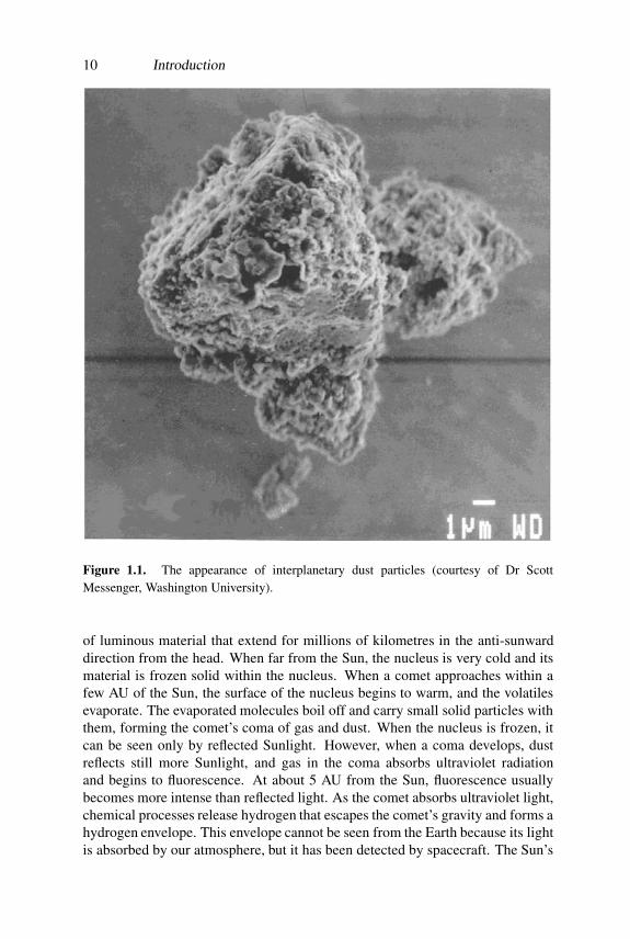
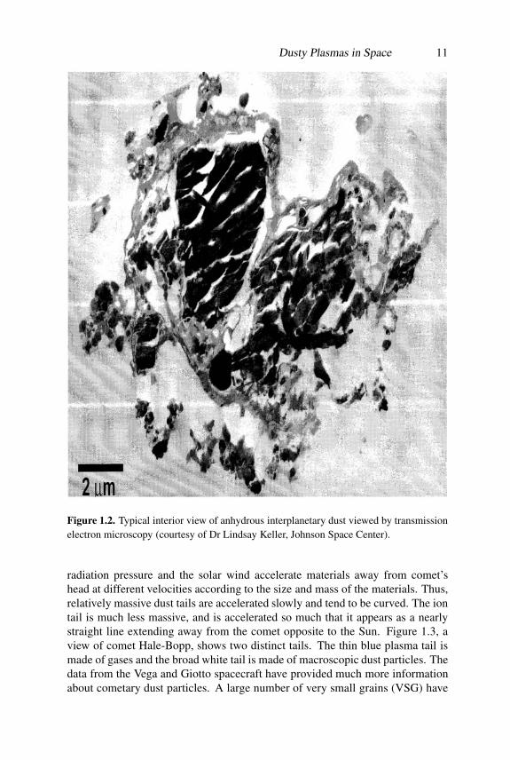
The interplanetary space is full of dust known as ‘interplanetary dust’. Theexistence of interplanetary dust particles was known from the zodiacal light.The zodiacal light is due to dust grains distributed throughout the inner solarsystem, with strong contributions from the asteroid belt. These have probablyoriginated from decay by collisional fragmentation of debris from comets, whichare known to release between 0.25 tonnes s−1 (in the case of short-period comets)and 20 tonnes s−1 (in the case of long-period comets) dusty gases in the solarsystem (de Angelis 1992). The other important sources of the interplanetarydust are asteroids that produce most of their dust during mutual collisions inthe asteroid belt. Through the combined effects of solar wind drag and thePoynting–Robertson light drag (a loss of orbital angular momentum by gyratingparticles associated with their absorption and re-emission of the solar radiation),all particles smaller than ∼1 cm gradually spiral into the Sun on timescalesranging from thousands to millions of years. It has been estimated that theaccretion of interplanetary dust (received by the Earth) is roughly 40 000 tonnesper year. For the past two decades NASA has routinely collected interplanetarydust in the stratosphere using high-altitude research aircrafts. The dust particlesare collected at altitudes of 18–20 km by inertial impacts onto plastic plates coatedwith highly viscous silicone oil. The size of most dust particles found on thecollectors are 5–20 mm. The interplanetary dust particles often have very fragile,fluffy appearance. The outside and inside of such interplanetary dust particles areshown in figures 1.1 and 1.2, respectively. Some of these particles are so fragilethat they disintegrate into dozens or hundreds of fragments when they impactthe collector surface. The interplanetary dust particles are usually very rich incarbon. Otherwise, they are usually composed of submicrometre mineral grains(hydrous or anhydrous), and some grains have abundant glassy modules (GEMS),proposed to be interstellar silicates. Typical parameters of dust-laden plasmasin the zodiacal dust disc are ne � 5 cm−3, Te � 105 K, nd � 10−12 cm−3,rd = 2 − 10 µm and a/λD � 5. There are many particles that appear to containabundant pre-solar molecular cloud material, marked by isotopic anomalies in Hand N (Messenger 2000).
1.3.2 Comets
Comets are small, fragile, irregularly shaped bodies composed of an admixture ofnon-volatile grains and frozen gases. They have highly elliptical orbits that bringthem very close to the Sun and swing them deeply into the space. The cometstructures are diverse and very dynamic, but they all develop a surrounding cloudof diffuse material, called a coma that usually grows in size and brightness as thecomet approaches the Sun. There is a small, bright nucleus (less than 10 km indiameter) in the middle of the coma. The coma and the nucleus together constitutethe head of the comet. As comets approach the Sun, they develop enormous tails
10 Introduction
Figure 1.1. The appearance of interplanetary dust particles (courtesy of Dr ScottMessenger, Washington University).
of luminous material that extend for millions of kilometres in the anti-sunwarddirection from the head. When far from the Sun, the nucleus is very cold and itsmaterial is frozen solid within the nucleus. When a comet approaches within afew AU of the Sun, the surface of the nucleus begins to warm, and the volatilesevaporate. The evaporated molecules boil off and carry small solid particles withthem, forming the comet’s coma of gas and dust. When the nucleus is frozen, itcan be seen only by reflected Sunlight. However, when a coma develops, dustreflects still more Sunlight, and gas in the coma absorbs ultraviolet radiationand begins to fluorescence. At about 5 AU from the Sun, fluorescence usuallybecomes more intense than reflected light. As the comet absorbs ultraviolet light,chemical processes release hydrogen that escapes the comet’s gravity and forms ahydrogen envelope. This envelope cannot be seen from the Earth because its lightis absorbed by our atmosphere, but it has been detected by spacecraft. The Sun’s
Dusty Plasmas in Space 11
Figure 1.2. Typical interior view of anhydrous interplanetary dust viewed by transmissionelectron microscopy (courtesy of Dr Lindsay Keller, Johnson Space Center).
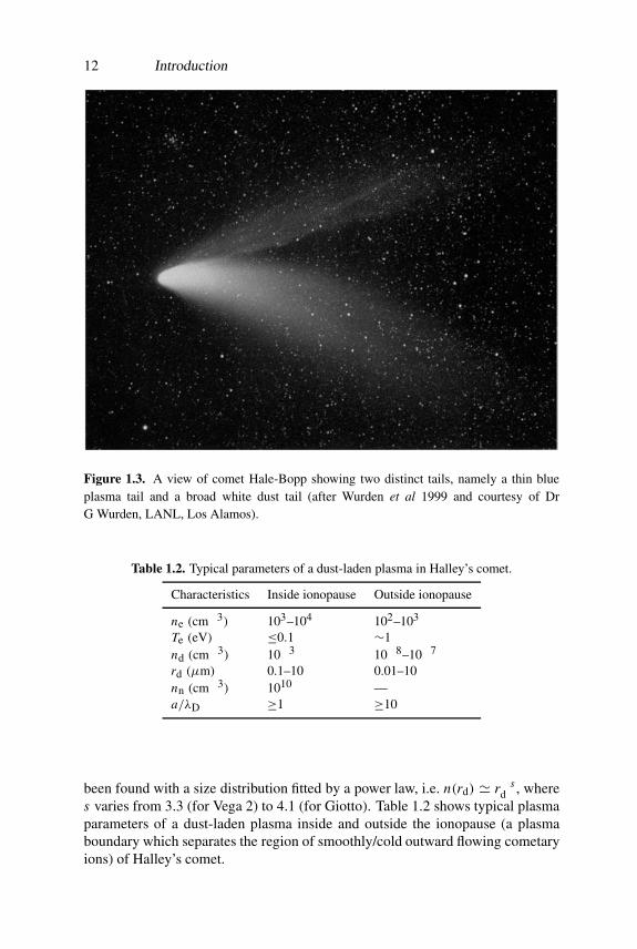
radiation pressure and the solar wind accelerate materials away from comet’shead at different velocities according to the size and mass of the materials. Thus,relatively massive dust tails are accelerated slowly and tend to be curved. The iontail is much less massive, and is accelerated so much that it appears as a nearlystraight line extending away from the comet opposite to the Sun. Figure 1.3, aview of comet Hale-Bopp, shows two distinct tails. The thin blue plasma tail ismade of gases and the broad white tail is made of macroscopic dust particles. Thedata from the Vega and Giotto spacecraft have provided much more informationabout cometary dust particles. A large number of very small grains (VSG) have
12 Introduction
Figure 1.3. A view of comet Hale-Bopp showing two distinct tails, namely a thin blueplasma tail and a broad white dust tail (after Wurden et al 1999 and courtesy of DrG Wurden, LANL, Los Alamos).
Table 1.2. Typical parameters of a dust-laden plasma in Halley’s comet.
Characteristics Inside ionopause Outside ionopause
ne (cm−3) 103–104 102–103
Te (eV) ≤0.1 ∼1nd (cm−3) 10−3 10−8–10−7
rd (µm) 0.1–10 0.01–10nn (cm−3) 1010 —a/λD ≥1 ≥10
been found with a size distribution fitted by a power law, i.e. n(rd) � r−sd , where
s varies from 3.3 (for Vega 2) to 4.1 (for Giotto). Table 1.2 shows typical plasmaparameters of a dust-laden plasma inside and outside the ionopause (a plasmaboundary which separates the region of smoothly/cold outward flowing cometaryions) of Halley’s comet.

Dusty Plasmas in Space 13
1.3.3 Planetary rings
It is now well established that most of the rings of the outer giant planets (such asJupiter, Saturn, Uranus, Neptune) are made of micron- to submicron-sized dustparticles. Below we provide a brief description for understanding the origin ofdust particles in planetary rings.
1.3.3.1 Jupiter’s ring system
The ring of Jupiter was discovered by Voyager 1 (by taking a single image) thatwas targeted specifically to search for a faint ring system. A more completeset of images were finally taken by Voyager 2. Jupiter’s ring is now known tobe composed of three major components, namely the main ring, the halo andthe gossamer ring. The main ring is about 7000 km wide and has an abruptouter boundary about 129 000 km from the centre of the planet. The main ringencompasses the orbits of the two small moons, Adrastea and Metis, which mayact as the source for the dust that makes up most of the ring.
1.3.3.2 Saturn’s ring system
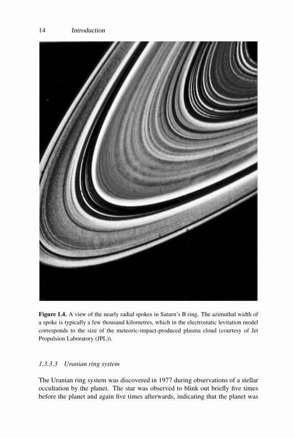
The rings of Saturn have puzzled astronomers since they were first discoveredby Galileo in 1610 using his first telescope. The puzzles have only significantlyincreased since Voyagers 1 and 2 imaged the ring system extensively in 1980 and1981. The rings have been given letter names in the order of their discovery. Themain rings (from the outward direction) are known as C, B and A. The CassiniDivision is the largest gap in the rings and separates the rings B and A. Recently, anumber of fainter rings have also been discovered. The D ring is exceedingly faintand closest to the planet. The F ring is narrow and just outside the A ring. Thereare two other far fainter rings named G and E. The particles in Saturn’s ringsare composed primarily of ice and range from microns to metres in size. One ofthe most interesting features observed in Saturn’s ring system by both Voyagers1 and 2 was the nearly radial spokes (Smith et al 1981, 1982) which (more thananything else) provided the impetus for the study of dust–plasma interactions inplanetary magnetospheres. These spokes are confined to the dense central B ringwith the inner edge at about 1.52Rs (Rs is the radius of Saturn) and the outer edgeat about 1.95Rs. They have an inner boundary at ∼1.72Rs and an outer boundaryat approximately the outer edge of the B ring. A typical spoke pattern is seen infigure 1.4. The spokes exhibit a characteristic wedge shape. The spoke model isbased on the assumption that the spokes contain electrostatically levitated micron-and submicron-sized dust grains and that the thin radial elongation is due to therapid radial motion of dense plasma clouds whose radii are of the order of severalthousand kilometres. The characteristics of dust and plasma varies from one ringto another. Table 1.3 shows the dust and plasma characteristics of the E ring, theF ring and the spokes of Saturn.
14 Introduction
Figure 1.4. A view of the nearly radial spokes in Saturn’s B ring. The azimuthal width ofa spoke is typically a few thousand kilometres, which in the electrostatic levitation modelcorresponds to the size of the meteoric-impact-produced plasma cloud (courtesy of JetPropulsion Laboratory (JPL)).
1.3.3.3 Uranian ring system
The Uranian ring system was discovered in 1977 during observations of a stellaroccultation by the planet. The star was observed to blink out briefly five timesbefore the planet and again five times afterwards, indicating that the planet was

Dusty Plasmas in Space 15
Table 1.3. Typical parameters of a dust-laden plasma in Saturn’s rings.
Characteristics E ring F ring Spokes
ne (cm−3) ∼10 ∼10 0.1–102
Te (K) 105–106 105–106 ∼104
nd (cm−3) 10−7 ≤10 ∼1rd (µm) ∼1 1 ∼1a/λD 0.1 ≤10−3 ≤10−2
encircled by five narrow rings. However, a number of Earth-based observationsindicated that there were actually nine major rings. These (from the outwarddirection) are 6, 5, 4, α, β, η, γ , δ and ε. A number of images, which provideadditional occultations of the ring system, were taken by the Voyager spacecraft in1986. The Voyager cameras also detected a few additional rings and showed thatthe nine major rings are surrounded by the belts of fine dust particles. A narrowring named 1986U1R or λ, which has been found to be different from the others,was discovered in the backscattered Voyager images. These rings observed in asingle Voyager image at high angles were found to be much brighter than theirenvironment. This indicates that the main constituent of these rings is dust. Oneother ring named 1986U2R, which is interior to all other rings, is also visible in asingle Voyager image at a phase angle of 90◦. Although it is not possible to obtainsufficient information about the particle properties of this ring from a single view,a predominance of dust is strongly suspected. To study the characteristics of theconstituents of Uranian rings, Ockert et al (1987) made a photometric analysisand showed that the brightness distribution is dominated by backscattering. Thisindicates that the rings mainly consist of macroscopic dust grains.
1.3.3.4 Neptune’s ring system
Neptune also has an external ring system. Earth-based observations showed onlyfaint arcs instead of complete rings. However, in the year 1989 Voyager 2’simages showed them to be complete rings with bright clumps. One of the rings(out of four) appears to have a curious twisted structure. Like those of Jupiterand Uranus, Neptune’s rings are very dark. The plasma wave instruments onboard the Voyager 2 spacecraft detected small micrometre-sized dust particles.Observations revealed a power law distribution (with an index 4) for the dustgrains. The dust radius was in the range 1.6–10 µm. The number density of thedust is very low (e.g. nd � 10−8–10−7 cm−3). The dust material is dirty ice,although other compositions (such as silicates) cannot be ruled out. Further studyis required to determine more accurately the mass and size distributions of dustgrains as well as charges residing on them. The data also revealed that at each ring

16 Introduction
plane there is an intense broadband burst of noise, extending from below 10 Hzto above 10 KHz. The presence of charged dust grains might be contributing tothese low-frequency noises in Neptune’s atmosphere which has oddly orientedmagnetic fields. The latter are presumably generated by motions of conductivefluids (probably water) in its middle layer.
1.3.4 Earth’s atmosphere
The most important part of our Earth’s environment, where the presence ofcharged dust particles are observed (Cho and Kelley 1993, Havnes et al 1996a),is the polar summer mesopause located between 80 and 90 km in altitude. Themost significant phenomenon observed in the polar summer mesopause is theformation of a special type of cloud known as ‘noctilucent clouds’ (NLCs). TheNLCs were reported for the first time in 1885 (Backhouse 1885) and were,from the beginning, recognized as being different from other clouds. Rocketgrenades launched during the International Geophysical Year of 1957–1958revealed another peculiarity of the polar mesopause: it was much colder in thesummer than in the winter. This observation supported speculations that theNLCs were composed of ice that formed at extremely low temperatures (evenbelow 100 K). There also occur some other important phenomena, such as thepolar mesospheric summer echoes (PMSE), and strong radar backscatter that hasbeen observed at frequencies from 50 MHz to 1.3 GHz. At the heights of thePMSE there also exist layers of electron density depletion and positive ion densityenhancement, which are elaborately discussed in some review articles (Thomas1991, Cho and Kelley 1993).
A number of more recent theories involve heavy ion clusters or charged dustparticles with total charge density that is significant compared with the electronor ion component (Havnes et al 1996a). A high charge density on the dust may,in principle, be the result of comparatively few and large highly charged dustparticles. A high charge on a dust particle can be possible only if the dust ispositively charged by photoemission. On the other hand, if the photoelectronemission is negligible and the dust grain charging is only due to collection ofplasma particles, the charge on each dust particle will be low (typically a fewunit charges or less) and negative (Havnes et al 1996a). Typical parameters ofdust-laden plasmas in NLCs are ne � 103 cm−3, Te � 150 K, nd � 10 cm−3,rd � 0.1 µm, nn � 1014 cm−3 and a/λD � 0.2.
One of the most significant sources of dust in the Earth’s atmosphere is man-made pollution (terrestrial aerosols). These have been found to be mainly (90%)in the form of aluminium oxide (Al2O3) spheroid in sizes that range from 0.1 µmto 10 µm. Their origin is from rocket and space shuttle exhausts (Bernhardt et al1995).
Recent measurements from balloon and aircraft collection have providedsome basic properties (such as constituents, size, density, etc) of dust particles inour Earth’s surroundings. These are listed in table 1.4. The characteristics of the

Dusty Plasmas in Laboratories 17
Table 1.4. Composition, size and density of dust particles in our Earth’s surroundings.
Origin Composition Radius (µm) Density (cm−3)
Shuttle exhausts dirty ice 5× 10⁻³ 3× 10⁴
Terrestrial aerosol Al2O3 spheroid 0.1–10 10−10–10−6
Micrometeoroid 60% chondritic, 5–10 10−10–10−9
30% iron–sulfur–nickel,10% silicates
Industrial magnetite spherules ∼10 ∼10−5
contamination
Table 1.5. Approximate values of some parameters of a dust-laden plasma in rocketexhausts and flames.
Characteristics Rocket exhausts Flames
ne (cm−3) 1013 1012
Te (K) 3× 10³ 2× 10³
nd (cm−3) 108 1011
rd (µm) 0.1 0.01nn (cm−3) 1018 1019
a/λD ≤5 ≤1
plasma and dust particles vary depending on the situation we consider. Table 1.5shows the characteristics of the plasma and dust particles in rocket exhausts andflames.
1.4 Dusty Plasmas in Laboratories
The extensive literature on dust in space and astrophysical plasmas (discussedin the preceding section) is a terrific starting point for the understandingof laboratory dusty plasmas. However, there are two distinctive featuresof laboratory dusty plasmas which differ significantly from those of spaceand astrophysical dusty plasmas. First, laboratory discharges have geometricboundaries whose structure, composition, temperature, conductivity, etc influencethe formation and transport of the dust grains. Second, the external circuit,which maintains the dusty plasma, imposes spatiotemporally varying boundaryconditions on the dusty discharge. We will now discuss how dust may occur
18 Introduction
in laboratory devices, particularly in direct current (dc) and radio-frequency(rf) discharges, plasma processing reactors, fusion plasma devices, solid-fuelcombustion products, etc.
1.4.1 dc and rf discharges
While dust particles are found in dc discharges, they are usually observed inlarger quantities for the same gases under conditions of rf excitations. Anobvious question may first arise: how do the dust particles originate? The dustparticles may originate from the plasma chemistry in the gas phase (e.g. carbonmonoxide or silane containing discharges) or from the sputtering of electrodes(e.g. most metals, graphite, etc). It is found that the dust particles occur morerapidly in electronegative gas mixtures or in a gas mixture where a substrate(such as silicon or carbon) is present. By the process of sputtering both siliconand carbon yield electronegative free radicals. To satisfy ambipolarity, the dustparticles will, therefore, be negatively charged. The rf discharge is a very efficienttrap for negative ions and for macroscopic, negatively charged dust particles.The electrodes acquire a negative dc bias due to the much higher mobility ofthe electrons compared with that of the positive ions. The ambipolar electricfields, which occur in the radial direction because of the mobility effect, alsotrap negative ions and dust particles. The physical properties (such as growth,charge, position, temperature, etc) of the dust particles, which are formed in dcor rf discharges, depend on various physical and chemical processes/parametersinvolved. These are pointed out as follows (Garscadden et al 1994).
(i) Growth: radicals and ion fluxes, bonds, temperature, desorption, surfacecharge, sputtering, etc.
(ii) Charge: floating potential, electron and ion fluxes, electron affinity andwork function, electrostriction, field and thermionic emission, photoelectriccharging, etc.
(iii) Position: electrostatic–gravitational balance, collisional drag from ions andneutrals, ensemble polarizability, mass, etc.
(iv) Temperature: surface radical recombination, surface electron–ion recombi-nation, surface quenching of energetic species, thermionic emission, pyroly-sis, radiation, Knudsen or continuum cooling, etc.
1.4.2 Plasma processing reactors
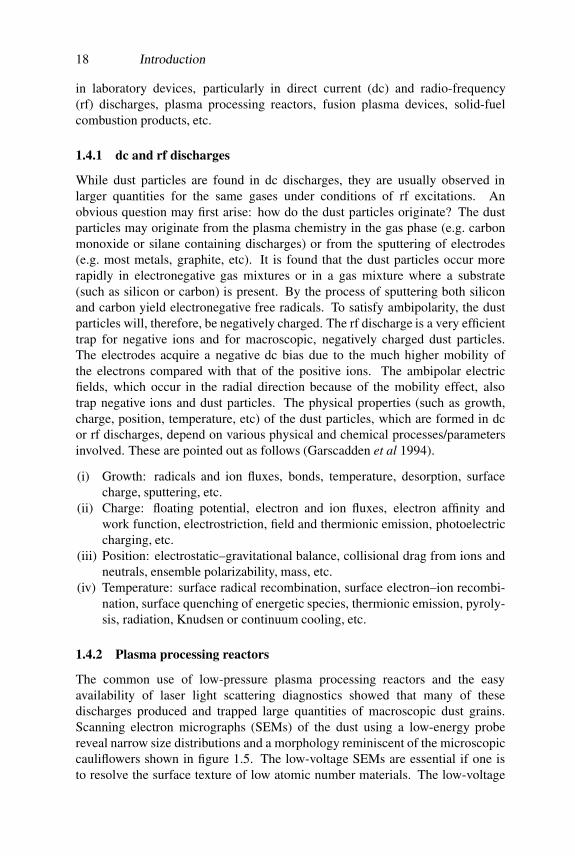
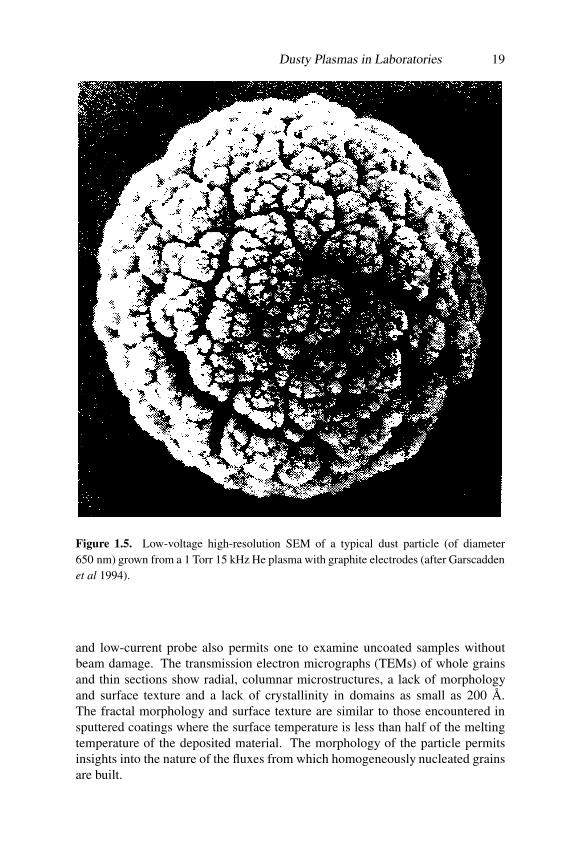
The common use of low-pressure plasma processing reactors and the easyavailability of laser light scattering diagnostics showed that many of thesedischarges produced and trapped large quantities of macroscopic dust grains.Scanning electron micrographs (SEMs) of the dust using a low-energy probereveal narrow size distributions and a morphology reminiscent of the microscopiccauliflowers shown in figure 1.5. The low-voltage SEMs are essential if one isto resolve the surface texture of low atomic number materials. The low-voltage
Dusty Plasmas in Laboratories 19
Figure 1.5. Low-voltage high-resolution SEM of a typical dust particle (of diameter650 nm) grown from a 1 Torr 15 kHz He plasma with graphite electrodes (after Garscaddenet al 1994).
and low-current probe also permits one to examine uncoated samples withoutbeam damage. The transmission electron micrographs (TEMs) of whole grainsand thin sections show radial, columnar microstructures, a lack of morphologyand surface texture and a lack of crystallinity in domains as small as 200 A.The fractal morphology and surface texture are similar to those encountered insputtered coatings where the surface temperature is less than half of the meltingtemperature of the deposited material. The morphology of the particle permitsinsights into the nature of the fluxes from which homogeneously nucleated grainsare built.

20 Introduction
1.4.3 Fusion plasma devices
The presence of dust particles in fusion devices has been known for a long time.However, their possible consequences for plasma operation and performanceshave become a topic of recent interest (Tsytovich 1997, Winter 1998, 2000). Theplasmas in fusion devices (for example, tokamaks, stellarators, etc) are more orless contaminated by elements (impurities) heavier than the hydrogen isotopeswhich are the fuel in fusion reactors. The impurities (dust particles) are generatedby a number of processes, such as desorption, arcing, sputtering, evaporation andsublimation of thermally overloaded wall material, etc. It is well known that inthe case of graphite wall components, in addition to C atoms, a significant amountof C1,C2,C3, . . . ,Cn clusters are liberated. The other generation mechanism forthe formation of impurities (dust particles) is the spallation and flaking of thinfilms of redeposited material or of films which were grown intentionally for wallconditioning purposes. The films from wall conditioning, which have a thicknessof a few 100 nm, can be the source of thin flakes. The redeposited layers fromtokamak operation may have thicknesses up to several 100 µm. They may have astratified structure due to the superposition of consecutive discharge events. Theytend to be mechanically unstable for thicknesses exceeding a few µm.
When we consider fusion devices operating with DT, additional processessuch as the formation of 3He due to the decay of T, the formation of 4He dueto neutron-induced spallation reactions of low-Z wall material, the ejection ofdust particles due to α-particle-induced embrittlement of the near-surface region,etc may become important. The dust particles are likely to be formed duringHe-glow discharge cleaning and during thin film deposition for wall conditioning(carbonization, boronization, siliconization). All particles that have been formedwill fall to the bottom at the end of a fusion plasma discharge. However, thelighter ones can be re-ejected into the fusion plasma either by magnetic effects orby electrostatic charging when they are in contact with the edge of the plasma.They may then be levitated close to the wall.
Recently, different types of dust particles were collected from the TEXTOR-94 which is a medium-sized tokamak with ∼4 MW ICRF and ∼4 MW neutralbeam injection heating and capable of full-performance plasma pulses withdurations up to 10 s (Winter 1998). The dust was collected by means of avacuum cleaner from the bottom porthole areas of TEXTOR-94. The coarseparticles were removed from the sticky bag of the vacuum cleaner by shakingthem off (coarse fraction). The main part of the coarse fraction consisted ofdark or whitish particles of typically 0.1–0.5 mm size with irregular shapes. Aninteresting point is that about 15% of these coarse particles are ferromagnetic. Arepresentative fraction of the magnetic coarse fraction is shown in figure 1.6. Thecoarse particles are found to be of different types and sizes, such as metal cuttings,spheres of diameters between 0.01 and 0.1 mm, irregularly formed pieces, etc.
The non-magnetic coarse particles, which appear like pieces of rock and witha composition of about 70% Si, 11% Al, 10% S, 7% Ca and 0.6% Fe, were also

Dusty Plasmas in Laboratories 21
Figure 1.6. An SEM image of magnetic coarse fraction showing metal cuttings, variousspheres and irregularly formed particles (after Winter 1998).
observed. These particles do not show the typical signatures of redeposited andflaked-off particles. They were probably formed during Si-ICRF conditioningor in test-limiter experiments with silane gas puffing, either by plasma-inducedgrowth or by pyrolysis and agglomeration in the plasma, or arc chipping fromvery thick local deposits (e.g. the test limiter). The co-deposited flaked-off filmsconstitute another part of the coarse non-magnetic fraction and resemble closelythat of their magnetic counterparts with the exception of a lower metal content.The third group of non-magnetic big particles was graphite grains with size of∼0.1 mm, composed of well established graphite grains with typical diameters of1–10 µm. These clearly originate from fatigued graphite armour tiles.
The particles from solvents (with suspended particles) taken immediatelyafter ultrasonic stir-up and those taken after 2 h of settlement differed in the sizedistribution. The particles taken after 2 h settlement were significantly smalleron average than the others. The smallest ones were partly ferromagnetic. Anumber of particles of submicron size, which themselves are agglomerates ofindividual particles of about 100–300 nm diameter, were found to exist. Theagglomerates are not always closely packed but have a woolly open structure.The size and structure of these small particles are consistent with what one wouldexpect from plasma-induced growth. The SEM investigations of nano-particlesformed in processing plasmas show similar sizes and a diffuse cauliflower-likestructure (shown in figure 1.5).

22 Introduction
Figure 1.7. Diagram of the main zones of the solid-fuel combustion product plasma (afterSamaryan et al 2000).
Table 1.6. Typical parameters of different regions in a solid-fuel combustion productplasma (Samaryan et al 2000).
Characteristics Flame region Boundary region Condensation region
Gas temperature (K) ∼3000 ∼2000 ∼600nd (cm−3) ≤102 103–108 ≥104
�c �1 3–40 �1
1.4.4 Solid-fuel combustion products
The presence of micron- or submicron-sized dust particles is experimentallyobserved in a solid-fuel combustion product plasma. Figure 1.7 shows a diagramof three main regions of a solid-fuel combustion product plasma (Samaryan etal 2000) which is produced by the combustion of the aluminium-coated solidfuel. The combustion product plasma consists of electrons, ions and micron-sized dust particles of a condensed dispersed phase. The magnesium-coatedsolid fuel may also be used to produce such a combustion product plasma. Theconstituents of dust particles are Al2O3 (in the case of aluminium-coated solidfuel) or MgO (in the case of magnesium-coated solid fuel). The number densityof alkile metal atoms ranges from ∼109 cm−3 to ∼1010 cm−3. The size of thedust particles is ∼0.2 µm. The other dusty plasma parameters in three mainregions of the solid combustion product plasma, namely the flame, boundaryand condensation regions, are given in table 1.6. It is well known that for agiven size and density of dust particles of the condensed dispersed phase theCoulomb coupling parameter �c is determined by the screening of the particlesby the plasma component formed as a result of the ionization of alkali-metal

Production of Dusty Plasmas 23
Figure 1.8. Diagram of the Q-machine including the rotating drum and the dust dispenser(after Merlino et al 1998).
impurity (Na and K which are always present in the synthetic fuel and end upin the combustion products) atoms. The plasma parameters in the flame andcondensation regions of the synthetic solid-fuel combustion product plasma aresuch that the Coulomb coupling parameter �c is much less than 1. Thus, inthese regions ordered structures of dust particles were not observed. The mainobstacle for the formation of ordered structures is a large amount of alkali-metalimpurities in the fuel samples, i.e. high electron and ion densities in a plasmaby ionization. A low density of dust particles of the condensed disperse phasein a high-temperature region was also an inhibiting factor. Ordered structures ofparticles of the condensed disperse phase were not observed in the condensationzone where the particle density is quite high, but the charge on the dust particles isso low on account of the relatively low temperature of the medium. However, foraluminium-coated solid fuels with a low alkali-metal impurity content, an orderedarrangement of the dust particles of the condensed dispersed phase may be formedin the boundary region between the flame and the condensation zone.
1.5 Production of Dusty Plasmas
To produce/confine dusty plasmas in laboratories, a number of techniques havebeen developed in the last few years. We now briefly explain some of thesetechniques/methods.
1.5.1 Modified Q-machine
A simple device for producing dusty plasmas is a dusty plasma device (DPD)which is a single-ended Q-machine modified to allow the dispersal of dust grains
24 Introduction
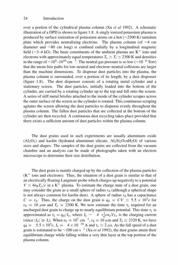
over a portion of the cylindrical plasma column (Xu et al 1992). A schematicillustration of a DPD is shown in figure 1.8. A singly ionized potassium plasma isproduced by surface ionization of potassium atoms on a hot (∼2500 K) tantalumplate which provides neutralizing electrons. The plasma column (of ∼4 cmdiameter and ∼80 cm long) is confined radially by a longitudinal magneticfield (∼3–4 kG). The basic constituents of the ambient plasma are K+ ions andelectrons with approximately equal temperatures Te � Ti � 2300 K and densitiesin the range of∼105–1010 cm−3. The neutral gas pressure is so low (∼10−6 Torr)that the mean free paths for ion–neutral and electron–neutral collisions are largerthan the machine dimensions. To dispense dust particles into the plasma, theplasma column is surrounded, over a portion of its length, by a dust dispenser(figure 1.8). The dust dispenser consists of a rotating metal cylinder and astationary screen. The dust particles, initially loaded into the bottom of thecylinder, are carried by a rotating cylinder up to the top and fall onto the screen.A series of stiff metal bristles attached to the inside of the cylinder scrapes acrossthe outer surface of the screen as the cylinder is rotated. This continuous scrapingagitates the screen allowing the dust particles to dispense evenly throughout theplasma column. The fallen dust particles that are collected at the bottom of thecylinder are then recycled. A continuous dust recycling takes place provided thatthere exists a sufficient amount of dust particles within the plasma column.
The dust grains used in such experiments are usually aluminium oxide(Al2O3) and kaolin (hydrated aluminium silicate, Al2Si2O7nH2O) of varioussizes and shapes. The samples of the dust grains are collected from the vacuumchamber and an analysis can be made of photographs taken with an electronmicroscope to determine their size distribution.
The dust grain is mainly charged up by the collection of the plasma particles(K+ ions and electrons). Thus, the situation of a dust grain is similar to that ofan electrically floating Langmuir probe which charges up negatively to a potentialV � 4kBTe/e in a K+ plasma. To estimate the charge state of a dust grain, onemay consider the grain as a small sphere of radius rd (although a spherical shapeis not always common for kaolin dust). A sphere of radius rd has a capacitanceC = rd. Thus, the charge on the dust grain is qd = CV � 5.5 × 10³e forrd = 10 µm and Te = 2300 K. We now estimate the time τc required for anuncharged dust grain to charge up to nearly equilibrium potential. This time τc isapproximated as τc = qd/Ie, where Ie ∼ −4πr2
d eneVT e is the charging current(since |Ie| � Ii). When ne = 107 cm−3, rd = 10 µm and Te � 2320 K, we haveqd = −5.5× 10³e, Ie = −4× 10⁻¹⁰ A and τc � 2 µs. As the fall speed of a dustgrain is estimated to be ∼100 cm s−1 (Xu et al 1992), the dust grains attain theirequilibrium charge while falling within a very thin layer at the top portion of theplasma column.

Production of Dusty Plasmas 25
Figure 1.9. Schematic illustration of how dusty plasmas are produced in strata of a dcneon glow discharge (after Fortov et al 1997).
1.5.2 dc discharges
Dusty plasmas are produced by suspending micron-sized dust particles in astratum of a dc neon glow discharge (Fortov et al 1997). The discharge is formedin a cylindrical glass tube with cold electrodes. A 3 cm inner diameter and60 cm long glass tube is positioned vertically. The electrodes are separated by40 cm. The discharge current is varied from 0.4 to 2.5 mA, the pressure of neonis varied from 0.2 to 1 Torr. These conditions allow the formation of the naturalstanding strata in between two electrodes as shown in figure 1.9. A few gramsof micron-sized particles are placed in a dust dropper in the upper side of theglass tube. The falling particles are trapped and suspended in the strata wherethe gravitational force mdg = ZdeEs (g is the acceleration due to gravity andEs is the electric field in the strata). Fortov et al (1997) used two types of dustgrains in their experiments, namely borosilicate glass micro-balloons and aluminaparticles, both having the mass density 2.3 g cm−3. The other parameters for suchdusty plasmas are Te = (3–30) × 104 K, ne � 109 cm−3, nd = 103–104 cm−3,Td = 300 K (room temperature), Es � 10 V cm−1, rd = 1–5 µm and Zd ∼ 105
(for alumina particles), rd = 50–65 µm and Zd � 106 (for glass particles).

26 Introduction
Figure 1.10. Sketch of the side view of the cylindrical discharge system (after Chu and I1994).
1.5.3 rf discharges
A dusty plasma has been for the first time confined in a cylindrical symmetricrf plasma system (Chu and I 1994). The system, the side view of which isshown in figure 1.10, consists of a hollow outer electrode capacitively coupledto a 14 MHz rf power amplifier, a grounded centre electrode with a ring-shapedgroove on the top for particle trapping and a top glass window for observation.A digital video recording system is used to monitor the image of the particlesilluminated by a He–Ne laser through an optical microscope mounted on the topof the chamber. The optical axis is parallel to the symmetry axis of the system.The system is pumped by a diffusion pump. O2 and SiH4 are introduced intothe chamber with 10 mTorr background argon gas. The ratio of the reactivegas flow to the partial pressure is kept 0.2 (cm3 min−1) mTorr−1. The O2 andSiH4 partial pressures are kept equal. The rf power is kept at 30 W. The systemtotal pressure is always kept less than 10 mTorr for the particle generation. Anaxial magnetic field (50–100 G) is also introduced to increase the generationefficiency. The particle size and number density increase with the reactive gasflow on time and pressure. After the formation of micron-sized particles, thereactive gas flows and the magnetic field is turned off. The particles are thentrapped in the toroidal groove. Under the gravitational force, the particle diameterslowly increases with decreasing hight. The size of the particles is almost mono-dispersive within 3 mm along the vertical direction. The rf power preciselycontrolled by a programmable function generator is the main control parameter.It has been observed in such an experiment that at low rf power the dust particlesare in the form of Coulomb crystals. However, as the rf power is increased, suchcrystals are melted.
Electrostatic Sheath 27
The dusty plasma parameters, which are obtained from the micro-imageand Langmuir probe measurements, are ne � 109 cm−3, nd = 2× 105 cm−3,rd = 5 µm (SiO2 particles), Te � 23 200 K, Ti � 350 K and �c = 100–200.
1.6 Electrostatic Sheath
It is now clear that in all laboratory plasma devices the plasma is confined withinfinite solid boundaries (walls). The behaviour of the plasma near the walls (whichis different from that away from the walls) in a two-component electron–ionplasma is well explained in some standard textbooks (Chen 1974). To understandthe behaviour of dusty plasmas near the boundary walls, we consider a one-dimensional model with no appreciable electric field inside the plasma. Weassume that the dusty plasma consists of thermal electrons, a cold ion fluid andnegatively charged immobile dust grains. If the electrons and ions hit the wall atthe same time, they combine and are lost. However, as the electrons have muchhigher thermal velocities than ions, they are lost faster than the ions and cause theboundary potential to be negative. This potential cannot be distributed over theentire plasma, since the Debye shielding will confine the potential variation to alayer of the order of several Debye lengths in thickness. This layer, which mustexist on all cold boundary walls (with which the plasma is in contact), is called anelectrostatic sheath.
To examine the exact behaviour of the potential φs(x) in the sheath, weassume that at the plane x = 0 the ions are entering the sheath region from themain plasma with a drift speed vi0. These drifting ions are needed to accountfor the loss of ions to the wall from the region in which they were created byionization. In steady state, we have for the cold ions
nivi = ni0vi0 (1.6.1)
and12 mi(v
2i − v2
i0) = −eφs (1.6.2)
where ni0 is the number density of single-charged ions at x = 0 (i.e. where φs istaken to be zero). The electron number density ne is given by equation (1.2.3).Equations (1.2.3), (1.6.1) and (1.6.2) are completed by Poisson’s equation
d2φs
dx2= 4πe(ne + Zdnd − ni) (1.6.3)
and the macroscopic charge neutrality condition
Zdnd = ni0 − ne0. (1.6.4)
Combining equations (1.6.1) and (1.6.2) we have
ni = ni0
(1− 2eφs
miv2i0
)−1/2
. (1.6.5)

28 Introduction
Substituting equations (1.2.3), (1.6.4) and (1.6.5) into equation (1.6.3) we obtain
d2ψs
dξ2= δ
(1+ 2ψs
M2
)−1/2
− exp(−ψs)− (δ − 1) (1.6.6)
where ψs = −eφs/kBTe, ξ = x/λDe, M = vi0/cs , cs = (kBTe/mi)1/2
and δ = ni0/ne0. Equation (1.6.6) is the nonlinear equation describing thebehaviour of the electrostatic potential in a dusty plasma sheath. Multiplyingequation (1.6.6) by dψs/dξ and integrating once, we obtain
1
2
(dψs
dξ
)2
+ V (ψs) = 0 (1.6.7)
where V (ψs) is given by
V (ψs) = (δ − 1)ψs − exp(−ψs)− δM2(
1+ 2ψs
M2
)1/2
+ Cs (1.6.8)
and Cs is an integration constant which takes the value Cs = 1+ δM2 for ψs = 0and dψs/dξ = 0 at ξ = 0. Equation (1.6.7) can be regarded as an ‘energy integral’of an oscillating particle of pseudo-mass ‘1’, pseudo-position ‘ψs’, pseudo-speed‘dψs/dξ ’ and pseudo-potential (also known as the Sagdeev potential) ‘V (ψs)’.The nature of ψs in the plasma sheath can, therefore, be studied either by analysisof the Sagdeev potential V (ψs) or by the numerical solution of equation (1.6.7).Whatever the method one uses, because of the square root term in equation (1.6.8),there is a lower bound ψs = −M2/2 for the potential, at which the ion densitybecomes infinite. Without going into further numerical details of equation (1.6.7),we analyse V (ψs) for the small-amplitude limit (i.e. ψs � 1) which providessome useful information about how the nature of ψs in a dusty plasma sheathdiffers from that in an electron–ion (two-component) plasma. For the smallamplitude limit, we expand V (ψs) in a Taylor series and obtain
V (ψs) = C1ψ2s + C2ψ
3s . . . (1.6.9)
where C1 = (δ/M2 − 1)/2 and C2 = (1/3 − δ/M4)/2. It turns out that thesolution of equation (1.6.7) exists if C1 < 0. The latter yields
δ
M2 − 1 < 0. (1.6.10)
The condition (1.6.10) is the modified Bohm criterion in the dusty plasma underconsideration. It is clear that in the absence of the dust particles, δ = 1 and theBohm criterion for the electron–ion (two-component) plasma becomes M > 1,whereas in the presence of the dust particles we have δ > 1 so that the Bohmcriterion becomes M > Mc, where Mc =
√δ. This clearly explains how the
presence of the dust particles modifies the Bohm criterion or the critical Mach

Some Aspects of Dusty Plasmas 29
number Mc. Since δ is a function of nd0 and Zd, the Bohm criterion is modifiedby the dust particle number density. We find that as ne0 decreases (i.e. nd0 or Zdincrease), the critical Mach number Mc increases. The Bohm criterion dictatesthat ions entering the sheath from the main body of the plasma must have a superion acoustic speed, which is larger when the dust grains are present.
1.7 Some Aspects of Dusty Plasmas
The physics of dusty plasmas is a topic of growing importance, which has gainedmore and more interest over the last few years not only from the academic point ofview, but also from the view of its new aspects in space and modern astrophysics,semiconductor technology, fusion devices, plasma chemistry, crystal physics,biophysics, etc. In the following sections, we briefly discuss some of theseimportant aspects.
1.7.1 Space science and astrophysics
The basic physics and chemistry of dusty plasmas in space (such as in planetaryrings, in cometary tails, in interstellar clouds, etc) is similar to that of low-pressurelaboratory dusty plasmas, but we have already shown in sections 1.3 and 1.4 thatthe plasma conditions for space dusty plasmas can differ from those of laboratorydusty plasmas by huge orders of magnitudes. The first hint that dust particleswere charged by the space plasma particles might explain some heavenly featurescame in October 1980 when Voyager 1 sped past Saturn and sent back picturesof mysterious dark spokes (Smith et al 1981) sweeping around the B ring (theplanet’s largest and brightest ring). It was then proposed by Hill and Mendis(1981a) as well as by Goertz and Morfill (1983) that the spokes might be chargeddust and sculpted by electrostatic forces. Hill and Mendis (1981a) argued thatelectrons hurled into the ring by aurora-like processes near Saturn might haveelectrified the dust, while Goertz and Morfill (1983) attributed the electrificationto the burst of the plasma generated as micrometeoroids pelted the boulder ofthe ring. Both of these mechanisms would tend to produce spoke-like regions(shown in figure 1.4) of electrification, where electrostatic repulsion between dustparticles and the boulders would raise trails of the dust grains.
On the other hand, the way by which tiny dust particles were distributed inthe cometary tails could not be explained by gravity or by other forces (associatedwith Sunlight pressure) acting on uncharged dust grains of this size. The solarradiation pressure should push the dust grains directly outward from the Sun,introducing tail symmetry above and below the cometary orbital plane. Butthe spacecraft that intercepted Comet Halley found that the smaller dust grainsgathered on one side of that plane (Glanz 1994). This can be explained byassuming that the dust particles picked up an electric charge from the solar windand that the charged dust particles moving through the magnetic field feel aforce perpendicular to their direction of travel and to the field direction. As the

30 Introduction
pressure of the Sunlight is pushing the grains directly away from the Sun and themagnetic field of the solar wind spirals along the ecliptic plane like the groovesin a phonograph record, the charged grains should get pushed either upwardsor downwards with respect to the orbital plane of the comet depending on theircharge. The calculations of the interaction between the grains and the solar windplasma showed that it would tend to give the grains a negative charge and theresulting force would push them below the orbital plane—exactly where theywere observed.
The different physical and chemical processes become important in thesevarious space dusty plasma situations. For example, the electrostatic equilibriumof a solid grain in the solar system can be affected by the photoelectron emissiondue to the solar radiation (which we will discuss in detail in chapter 2). Ithas been shown by Goertz (1989) that this leads to an electrostatic equilibriumof the particles which can be both size and time dependent, with a possiblepositive charge for larger (rd � 6 µm) particles and a negative charge for smaller(rd � 1 µm) particles. These considerations play a key role in several aspects:
(i) The chance of two dust particles combining to form a larger particlefollowing a collision increases when the particles are oppositely charged.This is important in understanding the evolution of the grain-sizedistribution.
(ii) The grain motion in planetary rings is influenced by electrical forcesconnected with the grain’s charge. The Voyager observations of Saturn’srings revealed the existence of radially elongated (∼106 m) discs withlight-scattering properties that suggest that the rings contain small grains(about a micron or less). These spokes are described through a gravito-electrodynamics model which suggests that electrostatic forces may beresponsible for the rich structure observed in Saturn’s rings via the radialtransport of the grains.
One of the other important applications of dusty plasma physics is tounderstand how ambipolar diffusion and interstellar grains (both charged andneutral) regulate the formation and evolution of proto-stellar cores in interstellarmolecular clouds. The dynamics or even the presence of charged dust particles inthe interstellar molecular clouds (which is, in fact, a partially ionized dusty plasmawith a significant fraction of neutrals) may affect the gravitational contractionprocess which causes the collapse of the large interstellar clouds. The dustparticles, by the process of coagulation, turn out to be a dust ball which serves asa core, and around such cores the gaseous components of the cloud can collapse.Therefore, the presence or the dynamics of charged dust grains essentially playsa vital role in star formation via self-gravitational instability.
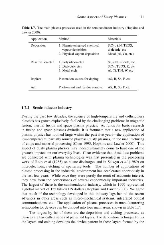
Some Aspects of Dusty Plasmas 31
Table 1.7. The main plasma processes used in the semiconductor industry (Hopkins andLawler 2000).
Application Method Materials
Deposition 1. Plasma-enhanced chemical SiO2, SiN, TEOS,vapour deposition dielectric, etc
2. Physical vapour deposition Metal (Al, Cu, etc)
Reactive ion etch 1. Polysilicon etch Si, SiN, silicide, etc2. Dielectric etch SiO2, TEOS, K, etc3. Metal etch Al, Ti, TiN, W, etc
Implant Plasma ion source for doping AS, B, Sb, P, etc
Ash Photo-resist and residue removal AS, B, Sb, P, etc
1.7.2 Semiconductor industry
During the past few decades, the science of high-temperature and collisionlessplasmas has grown explosively, fuelled by the challenging problems in magneticfusion, inertial fusion and space plasma physics. As funds for basic researchin fusion and space plasmas dwindle, it is fortunate that a new application ofplasma physics has loomed large within the past five years—the application oflow-temperature, partially ionized plasmas (dusty plasmas) in the manufacturingof chips and material processing (Chen 1995, Hopkins and Lawler 2000). Thisaspect of dusty plasma physics may indeed ultimately come to have one of thegreatest impacts on our everyday lives. Clear evidence that these dust problemsare connected with plasma technologies was first presented in the pioneeringwork of Roth et al (1985) on silane discharges and in Selwyn et al (1989) onmicroelectronics etching or sputtering tools. The number of applications ofplasma processing in the industrial environment has accelerated enormously inthe last few years. While once they were purely the remit of academic interest,they now form the cornerstones of several economically important industries.The largest of these is the semiconductor industry, which in 1999 representeda global market of 155 billion US dollars (Hopkins and Lawler 2000). We agreethat much of the technology developed in this industry lags behind the recentadvances in other areas such as micro-mechanical systems, integrated opticalcommunications, etc. The application of plasma processes in manufactureringsemiconductor devices can be divided into four main areas, shown in table 1.7.
The largest by far of these are the deposition and etching processes, asdevices are basically a series of patterned layers. The deposition technique formsthe layers and etching develops the device pattern in these layers formed by the
32 Introduction
lithography steps. These processes are also an integral part of the lithographysteps as they are used to form the reticles/masks used by the photo-lithographyprocess to pattern the device on the silicon wafers. There are two main typesof plasma systems used commercially: capacitively coupled and inductivelycoupled. There are also a number of electron cyclotron resonance sources andhelicons, though these are less common.
1.7.3 Plasma chemistry and nanotechnology
The field of dusty plasmas, which is in fact a multi-disciplinary researchtopic of recent interest, involves not only numerous physical processes, butalso deals with fundamental mechanisms and questions that arise in detailedphysics and chemistry leading to particle formation. The heterogeneous andhomogeneous nucleation phenomena determine the formation of very small(less than nanometre) sized proto-particles. The formation of proto-particles isfollowed by agglomeration and coagulation processes, as similarly found in otherparts of chemistry such as colloidal chemistry.
Basically the formation of powder in a reactive plasma starts with theformation of primary clusters of atoms which grow during a nucleation phaseup to a critical number density. The coagulation or agglomeration leads then tomacro-particles with size around 50 nm, which finally grow to micrometre-sizedparticles by accretion of neutrals or ionic monomers, since further agglomerationis prevented by the particle charging (Bouchoule 1999, Perrin and Hollenstein1999, Gallagher 2000, Hollenstein 2000). The powder formation is observedin most of the popular reactive plasmas that are used for industrial applications(Bouchoule 1999). The powder formation is not only found in hydrocarbonand silane plasmas, but also in plasmas with more complex monomers suchas hexamethyldisiloaxane or oxygen plasmas (Perrin and Hollenstein 1999,Hollenstein 2000). At present, the different mechanisms and processes leadingto powder formation in these reactive plasmas are far from being elucidated.The behaviour of larger particles (of radius larger than few tens of nanometres)produced in the process of powder formation is more or less well understood.However, on the formation and behaviour of the smaller proto-particles and theirchemistry only little is known; this is essentially due to experimental difficultiesin detecting and monitoring these small particles in detail. Besides the differentphysical and chemical processes leading to the formation of these proto-particlesor precursors, the nature of the nucleation process plays a primary role. Thenucleation process may be driven either by homogeneous or heterogeneousreactions. However, in many cases it is found to be very difficult to distinguishthe real origin of the nucleation and much research effort is at present spent onthis problem.
It is still believed that homogeneous reactions dominate the powderformation reactions in pure silane rf plasmas. The particle growth in these plasmasis thought to be a consequence of the strong electron-attachment energies of

Some Aspects of Dusty Plasmas 33
Si-containing molecules and particles (Perrin and Hollenstein 1999, Gallagher2000, Hollenstein 2000). Recently, a steady-state homogeneous model of particlegrowth in silane discharges has been proposed by Gallagher (2000) who assumedthat particles grow primarily from SiH−3 and SiHm radicals, first into Six H−mions and SixHm radicals, then with increasing x into clusters containing multiplybonded silicon, and finally into compact, primarily silicon particles.
A number of experimental investigations (Kushner 1988) has beenperformed in order to address the powder precursors in these plasmas and the gas-phase reactions leading to large clusters that finally agglomerate to form particlesup to a micrometre in size. The neutral radicals have been the candidates forparticle precursors since reaction path propagation is supposed to proceed bythe insertion of silane radicals into higher-mass saturated molecules (Hollenstein2000). The positive ions have also been invoked as potential powder precursors,although it has been found that activation barriers exist, preventing the formationof high-mass cations. The negative ions are also experimentally found to exist insilane plasmas (Hollenstein 2000). The experimental anti-correlation between thenegative ion intensity and the powder formation and their rf modulation frequencydependence indicate the importance of the anion trapping in this process. At lowerrf power modulation frequencies all the negative ions formed leave the dischargevolume, but at higher power modulation frequencies the plasma off time is tooshort to empty completely the discharge of the negative ions. Thus, in the lattercase a large fraction of the negative ions remains trapped and they accumulate andgrow towards higher and higher masses in a similar way as in the model recentlyconsidered by Gallagher (2000). It has been, therefore, proposed that negativeions may be the most possible powder precursors in a pure rf SiH4 plasma atlow or moderate power densities and that the polymerization pathway proceedsvia negative ion clustering. The possible path way for SiH4 addition reactionsproposed by Perrin and Hollenstein (1999) is
SinH−m + SiH4 −→ (Sin+1H−m′)∗ + (H,H2) products (1.7.1)
where excited negative ions (Sin+1H−m′)∗ may relax either by redistribution of
excess energy among internal re-vibrational modes or by stabilizing collisionswith a third body with their auto-detachment lifetime
(Sin+1H−m′)∗ + M −→ Sin+1H−m′ +M. (1.7.2)
The mutual anion–cation recombinations as given by
SinH−m + SipHq −→ Sin′Hm′ + (H,H2) products (1.7.3)
followed by re-attachment of an electron on the recombined neutral
e+ Sin′Hm′ −→ (Sin′Hm′)∗ −→ Sin′Hm′ (1.7.4)
may be a second possible polymerization path as proposed by Haaland (1990).The agglomeration, as often observed in dusty plasmas, is a fundamental

34 Introduction
process which plays an important role in many parts of physics, chemistryand astrophysics (Horanyi and Goertz 1990). After a first phase, where theplasma chemistry dominates, a few nanometre-sized primary particles or proto-particles are formed. They reach a critical number density that triggers a rapidgrowth or an agglomeration phase. Within a short time the particle size stronglyincreases up to a few hundred nanometres, whereas the particle number densitydecreases drastically over several orders of magnitude. The agglomeration andits different forms such as coagulation and flocculation are the basic phenomenain colloidal systems such as aerosols (Bouchoule 1999, Perrin and Hollenstein1999, Hollenstein 2000). It has been assumed in most of the previous models foragglomeration in dusty plasmas that the agglomerating particles are electricallyneutral and so all classes of particles can agglomerate with each other. However,particles in the plasma, especially particles of several nanometres or larger insize are necessarily electrically charged. The particle charging might reducethe agglomeration rate and also influence the limit of the maximum achievableparticle size. Recently, a few attempts have been made in order to include thecharging into an agglomeration model (Kortshagen and Bhandarkar 1999, Kimand Kim 2000).
1.7.4 Fusion research
We have already discussed in section 1.4.3 the properties of dust grains and theiroccurrence in fusion devices. The dust is indeed an important safety issue forITER and future fusion reactors. The dust particles may retain a large fraction ofhydrogen (>0.2 H/C) which will lead to considerable tritium inventories (Winter1998, 2000). Furthermore, these fine dispersed dust particles may be chemicallyreactive and may spontaneously react with oxygen or water vapour in the case ofa vacuum or coolant leak. A further aspect is the migration of dust particles. Dueto thermophoretic forces and due to repetitive evaporation and condensation theymay accumulate at cold areas of the device. They may block spacings and fillgaps which were introduced for engineering reasons. The heat transfer to activelycooled components may be impeded by a loose dust layer on the surface.
The problem of dust in tokamaks is of growing interest now. The sizes ofthe dust particles, which are observed in tokamaks TEXTOR, DIII-D, ALCATORC-MOD, TFTR, etc, range from ∼100 nm to ∼100 µm (Winter 1998, 2000).The strongest evidence for a self-organized structure (Tsytovich 1997) of thetokamak dust is probably the fractal structures of the cauliflower-like forms shownin figure 1.5.
1.7.5 Crystal physics
The search for ordered many-body Coulomb systems in laboratory devices hasbeen a problem of great interest over the past few decades. The competitionbetween the mutual Coulomb interaction and the background thermal fluctuation
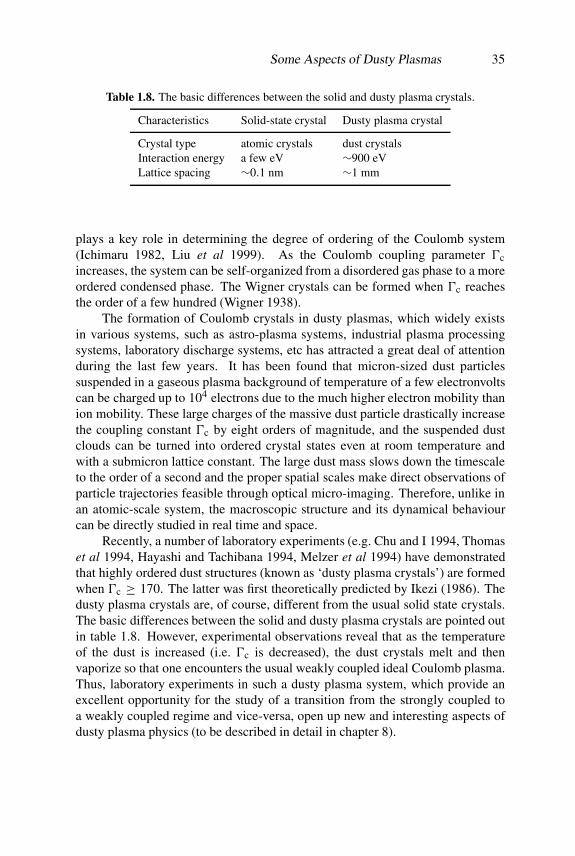
Some Aspects of Dusty Plasmas 35
Table 1.8. The basic differences between the solid and dusty plasma crystals.
Characteristics Solid-state crystal Dusty plasma crystal
Crystal type atomic crystals dust crystalsInteraction energy a few eV ∼900 eVLattice spacing ∼0.1 nm ∼1 mm
plays a key role in determining the degree of ordering of the Coulomb system(Ichimaru 1982, Liu et al 1999). As the Coulomb coupling parameter �cincreases, the system can be self-organized from a disordered gas phase to a moreordered condensed phase. The Wigner crystals can be formed when �c reachesthe order of a few hundred (Wigner 1938).
The formation of Coulomb crystals in dusty plasmas, which widely existsin various systems, such as astro-plasma systems, industrial plasma processingsystems, laboratory discharge systems, etc has attracted a great deal of attentionduring the last few years. It has been found that micron-sized dust particlessuspended in a gaseous plasma background of temperature of a few electronvoltscan be charged up to 104 electrons due to the much higher electron mobility thanion mobility. These large charges of the massive dust particle drastically increasethe coupling constant �c by eight orders of magnitude, and the suspended dustclouds can be turned into ordered crystal states even at room temperature andwith a submicron lattice constant. The large dust mass slows down the timescaleto the order of a second and the proper spatial scales make direct observations ofparticle trajectories feasible through optical micro-imaging. Therefore, unlike inan atomic-scale system, the macroscopic structure and its dynamical behaviourcan be directly studied in real time and space.
Recently, a number of laboratory experiments (e.g. Chu and I 1994, Thomaset al 1994, Hayashi and Tachibana 1994, Melzer et al 1994) have demonstratedthat highly ordered dust structures (known as ‘dusty plasma crystals’) are formedwhen �c ≥ 170. The latter was first theoretically predicted by Ikezi (1986). Thedusty plasma crystals are, of course, different from the usual solid state crystals.The basic differences between the solid and dusty plasma crystals are pointed outin table 1.8. However, experimental observations reveal that as the temperatureof the dust is increased (i.e. �c is decreased), the dust crystals melt and thenvaporize so that one encounters the usual weakly coupled ideal Coulomb plasma.Thus, laboratory experiments in such a dusty plasma system, which provide anexcellent opportunity for the study of a transition from the strongly coupled toa weakly coupled regime and vice-versa, open up new and interesting aspects ofdusty plasma physics (to be described in detail in chapter 8).
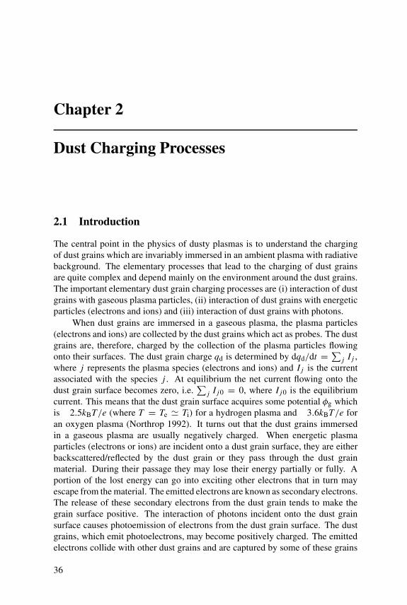
Chapter 2
Dust Charging Processes
2.1 Introduction
The central point in the physics of dusty plasmas is to understand the chargingof dust grains which are invariably immersed in an ambient plasma with radiativebackground. The elementary processes that lead to the charging of dust grainsare quite complex and depend mainly on the environment around the dust grains.The important elementary dust grain charging processes are (i) interaction of dustgrains with gaseous plasma particles, (ii) interaction of dust grains with energeticparticles (electrons and ions) and (iii) interaction of dust grains with photons.
When dust grains are immersed in a gaseous plasma, the plasma particles(electrons and ions) are collected by the dust grains which act as probes. The dustgrains are, therefore, charged by the collection of the plasma particles flowingonto their surfaces. The dust grain charge qd is determined by dqd/dt = ∑ j I j ,where j represents the plasma species (electrons and ions) and I j is the currentassociated with the species j . At equilibrium the net current flowing onto thedust grain surface becomes zero, i.e.
∑j I j0 = 0, where I j0 is the equilibrium
current. This means that the dust grain surface acquires some potential φg whichis −2.5kBT/e (where T = Te � Ti) for a hydrogen plasma and −3.6kBT/e foran oxygen plasma (Northrop 1992). It turns out that the dust grains immersedin a gaseous plasma are usually negatively charged. When energetic plasmaparticles (electrons or ions) are incident onto a dust grain surface, they are eitherbackscattered/reflected by the dust grain or they pass through the dust grainmaterial. During their passage they may lose their energy partially or fully. Aportion of the lost energy can go into exciting other electrons that in turn mayescape from the material. The emitted electrons are known as secondary electrons.The release of these secondary electrons from the dust grain tends to make thegrain surface positive. The interaction of photons incident onto the dust grainsurface causes photoemission of electrons from the dust grain surface. The dustgrains, which emit photoelectrons, may become positively charged. The emittedelectrons collide with other dust grains and are captured by some of these grains
36
Isolated Dust Grains 37
which may become negatively charged. There are, of course, a number of otherdust grain charging mechanisms, namely thermionic emission, field emission,radioactivity, impact ionization etc. These are significant only in some differentspecial circumstances.
To explain different important dust grain charging processes, we considerfirst isolated dust grains and then non-isolated dust grains. We also describe howthe dust grain charge (in both isolated and non-isolated cases) can be measured inlaboratory experiments. We finally discuss some important consequences of thedust grain charging processes.
2.2 Isolated Dust Grains
It is quite difficult to explain/understand the charging of a dust grain if all thecharging processes mentioned above are included simultaneously. We, therefore,consider small isolated dust grains (rd � λD � a) and explain each of theimportant dust grain charging mechanisms one by one.
2.2.1 Collection of plasma particles
We consider a finite-sized neutral dust particle immersed in an unmagnetizedplasma whose constituents are electrons and ions. Since the electron thermalspeed is much larger than the ion thermal speed, the electrons reach the dust grainsurface much more rapidly than the ions. Thus, the dust grain acquires much moreelectrons than ions, and as a result its surface potential becomes negative. On theother hand, absorption of the plasma ions tends to make the dust grain charge aswell as its surface potential positive. The currents of the primary electrons andions are, of course, affected by the grain surface potential itself, since they dependon the relative speed between the plasma and the dust grain. When the surfacepotential is negative, the electrons are repelled and the ions are attracted, i.e. thedust grain current carried by the electrons is reduced and that carried by the ions isincreased. On the other hand, if the surface potential is positive, the electrons areattracted and the ions are repelled, i.e. the grain current carried by the electrons isincreased and that carried by the ions is reduced.
We now calculate the charging current I j to the dust grain carried by theplasma particle j by using the orbit-limited motion (OLM) approach (Chen 1965,Allen 1992). We consider (as shown in figure 2.1) that from an infinite distancea plasma particle j is approaching a spherical dust grain of radius rd and chargeqd. When the plasma particle enters the Debye sphere, it feels the influence of thedust grain and its path changes due to the electrostatic force. We assume that v j
and vg j are the speed of the plasma particle before and after its grazing collisionwith the dust grain. It is obvious that for a fixed velocity, as we decrease theimpact parameter b j , the plasma particle hits the dust grain. The cross sectionfor charging collisions between the dust and the plasma particle j is σ d
j = πb2j .

38 Dust Charging Processes
Figure 2.1. Grazing collisions between a plasma particle j and a charged dust particlewith q j qd < 0.
Conservation of momentum and energy requires that
m jv j b j = m jvg j rd (2.2.1a)
and1
2m jv
2j =
1
2m jv
2g j +
q j qd
rd. (2.2.1b)
The dust grain charge qd is related to the potential difference φd(= φg − φp)
between the grain potential φg and the plasma potential φp, i.e. qd = Cφd,where the capacitance C of the spherical dust grain in a plasma is C =rd exp(−rd/λD) � rd for λD � rd. Using the relation qd = rdφd andequations (2.2.1a) and (2.2.1b) one can easily express b j in terms of φd. Thus,σ d
j becomes
σ dj = πr2
d
(1− 2q jφd
m jv2j
). (2.2.2)
If f j (v j ) is the velocity distribution of the plasma species j at infinite distancefrom the dust grain, the dust grain charging current I j carried by the plasmaspecies j is
I j = q j
∫ ∞
V minj
v jσdj f j (v j ) dv j (2.2.3)
where V minj is the minimum value of the plasma particle velocity for which the
particle hits the dust grain. To approximate V minj we consider two situations,
namely q jφd < 0 and q jφd > 0. When q jφd < 0, the plasma particle andthe dust grain attract each other and the integration in equation (2.2.3) is to beperformed over the complete v j domain. On the other hand, when q jφd > 0, theplasma particle and the dust grain repel each other and hence V min
j > 0 in order
Isolated Dust Grains 39
to allow for a collision between the dust grain and the plasma particle. Thus, inthis case V min
j becomes
V minj =
(−2q jφd
m j
)1/2
. (2.2.4)
We further assume that the velocity distribution of the plasma species isMaxwellian, i.e.
f j (v j ) = n j
(m j
2πkBTj
)3/2
exp
(− m jv
2j
2kBTj
)(2.2.5)
where n j is the plasma particle number density. Substituting equations (2.2.2) and(2.2.5) into equation (2.2.3), expressing the result in spherical polar coordinatesand performing the integration, we can write the charging current I j for attractive(q jφd < 0) and repulsive (q jφd > 0) potentials as
I j = 4πr2d n j q j
(kBTj
2πm j
)1/2 (1− q jφd
kBTj
)for q jφd < 0 (2.2.6)
and
I j = 4πr2d n j q j
(kBTj
2πm j
)1/2
exp
(−q jφd
kBTj
)for q jφd > 0. (2.2.7)
Equation (2.2.7) is valid for any repulsive potential in a Maxwellian plasma aslong as the surface potential has a monotonic behaviour outwards from the surfaceas well as when the streaming speed v j0 is much smaller than the thermal speedVT j . Now, we consider a more general dusty plasma situation in which the ionshave some finite streaming speed. For such a situation the electron current is asbefore, but the ion current will be different and can be calculated by using the iondistribution function
fi(vi) = ni
(mi
2πkBTi
)3/2
exp
[−mi(vi − vi0)
2
2kBTi
]. (2.2.8)
Thus, following the same procedure as before, we can obtain the ion current Ii.For negatively charged dust grains we have (Shukla 1996)
Ii = 4πr2d eni
(kBTi
2πmi
)1/2 [F1(u0)− F2(u0)
eφd
kBTi
](2.2.9)
where F1(u0) = (√π/4u0)(1 + 2u2
0) erf(u0) + (1/2) exp(−u20) and F2(u0) =
(√π/2u0) erf(u0) are written in terms of the error function erf(u0) =
(2/√π)∫ u0
0 exp(−t2) dt and u0 = vi0/VTi. It is easy to show by Taylor series

40 Dust Charging Processes
expansion around u0 = 0 that both the function F1 and F2 approach unity as u0approaches zero. Thus, it is obvious that for ion streaming speed much less thanthe ion thermal speed, i.e. for u0 � 1, equation (2.2.9) reduces to equation (2.2.7)with j = i and qi = e. On the other hand, if the ion streaming speed ismuch larger than the ion thermal speed, i.e. if u0 � 1, the ion current can beapproximated as
Ii � πr2d enivi0
(1− 2eφd
mv2i0
). (2.2.10)
We discussed above the charging current for an orbit-limited sphere. Butwhat will be the corresponding charging current I j for an orbit-limited cylinder?The answer to this question was provided by Whipple (1981) who considered aMaxwellian distribution of plasma particles (electrons and ions) and showed thatthe charging current I j for an orbit-limited cylinder with q jφd < 0 is
I j = 2πrd Ldn j q j
(kBTj
2πm j
)1/2 2√π
[ψd +
√π
2exp(ψ2
d ) erfc(ψd)
](2.2.11)
where erfc(ψd) is the complementary error function defined as
erfc(ψd) = 2√π
∫ ∞
ψd
exp(−t2) dt (2.2.12)
ψd = (−q jφd/kBTj )1/2 and Ld is the length of the cylindrical dust grain. The
concept of the OLM can be further generalized to include collectors that are lesssymmetric than spheres and circular cylinders (Laframboise and Parker 1973).
We may also ask ourselves: how can we obtain the charging current thatis sheath-limited rather than orbit-limited? When the current is sheath-limited,the range of integration must be determined from the behaviour of the particletrajectories in the sheath. This is, in general, a complicated problem that can onlybe treated numerically by following particle orbits and by treating the potentialdistribution self-consistently.
2.2.2 Secondary electron emission
The energetic primary plasma particles falling onto a dust grain surface may causea release of secondary electrons from the latter. The process of secondary electronemission can occur in two ways: one by electron impact and the other by ionimpact. We now briefly discuss these two processes.
2.2.2.1 Electron impact
When an electron approaches a dust grain surface, it has to face any of thefollowing possible situations: it may be scattered/reflected by the dust grainbefore it enters into the dust grain, it may enter into the dust grain and
Isolated Dust Grains 41
stop immediately (i.e. stick onto the dust grain surface), it may enter intothe dust grain, interact with scattering centres and pass a part or all of thedust material wherein it may lose its energy, and a portion of this energycan go into exciting other electrons which in turn may escape from the grainsurface. These situations, namely reflection, absorption, transmission/tunnellingand secondary emission are usually treated as distinct processes. Reflectionor absorption is only significant for incident electrons with very low energies.The tunnelling/transmission refers to those electrons which leave the dust grainmaterial with a similar but somewhat lower energy than they had upon enteringthe dust grain. The tunnelling is experimentally distinguished from the secondaryemission primarily by the energy of the emitted electrons. The contribution ofthe processes of scattering/reflection and absorption/collection of primary plasmaparticles is described in the previous section. The present section is, therefore,concerned with the processes of tunnelling/transmission and secondary electronemission which directly lead to the charging of the dust grains.
We first discuss how one can obtain the expression for the secondaryemission yield from a spherical dust grain surface. The well known Sternglassformula (Sternglass 1954, Jonker 1952) for the secondary emission yield fromsemi-infinite slabs of material, where the electrons are assumed to escape fromonly one surface (the side at which the primary electrons enter), cannot be usedwhen dealing with different geometries other than a planar slab. For a situationof spherical dust grains the secondary electrons are not limited to the point ofincidence of primary electrons, but may also exit from all points of the grainsurface. Thus, the secondary emission yield for spherical dust grains is higherthan that determined by the Sternglass formula. Chow et al (1993) have modifiedthe yield equation of Jonker (1952) and have derived the modified yield equationfor the enhanced secondary emission yield from a very small spherical dust grain.
Chow et al (1993) have considered a very small spherical dust grain andhave assumed that (i) the energy loss of the primary electrons can be described byWhiddington’s law (Whiddington 1912): E(x) = (E2
p − KWx)1/2, where E(x)is the energy of the primary electron at a depth x (after entering into the dustgrain), Ep is the initial energy of the primary electron (just before entering intothe dust grain) and KW is Whiddington’s constant for energy loss with distance,(ii) the primary electron current density is conserved within the grain, (iii) theproduction of secondaries is proportional to the energy loss of the primaries, (iv)the secondary electron flux decreases exponentially with distance between thesurface and the point of production and (v) the primary electrons are incidentnormal to the grain. Using these assumptions we can express the current disassociated with the secondary electrons (excited by the primary electrons thathave traversed a distance from x to x + dx beneath the dust grain surface) as
dis = −Ks Iee−αl(x,θ) dE
dxdx (2.2.13)
where α is the inverse of the absorption length for secondaries, Ks represents

42 Dust Charging Processes
Figure 2.2. The model geometry for the secondary electron emission from a smallspherical dust grain (after Chow et al 1993).
the efficiency with which the lost primary electron energy is used to excite thesecondaries and l(x, θ) is the distance that a secondary electron must travel toreach the surface from a depth x and along an angle θ from the primary electronpath (as shown in figure 2.2). To determine the length l(x, θ), we neglect thecontribution of the scattering process and assume that the secondaries are emittedisotropically in all directions from the point of excitation (Jonker 1952). Thegeometry for the secondary electron emission shown in figure 2.2 allows us toexpress l(x, θ) as
l(x, θ) = [r2d + (rd − x)2 − 2rd(rd − x) cos θ ′]1/2 (2.2.14)
where θ ′ = θ − sin−1[(rd − x) sin θ/rd]. It is easily shown that the ratio of thesecondaries emitted at an angle θ in the range θ and θ + dθ to the total numberof excited secondaries is 0.5 sin θ dθ . It should be noted that, for a spherical dustgrain, θ can vary from 0 to π , whereas, for a planar slab, θ is limited to π/2. UsingWhiddington’s law, we can express the current dIs associated with the secondary
Isolated Dust Grains 43
electrons asdIs = 1
2 Ks KW Ie(E2p − KWx)−1/2 f (x) dx (2.2.15)
where
f (x) = 12
∫ π
0e−αl(x,θ) sin θ dθ (2.2.16)
with l(x, θ) given in equation (2.2.14). Since a primary electron excitessecondaries along its entire path within the grain, we must integrateequation (2.2.16) from the point of entry (x = 0) to either the point of exit(x = 2rd = Dg) or the maximum penetration distance, depending on which oneof the two values is smaller. The maximum penetration depth xmax correspondsto the point at which E(x) = 0 and can be determined from Whiddington’s law.The latter yields xmax = E2
p/KW. It is obvious that the primary electrons canonly escape the grain at the opposite side (x = Dg) when the primary electronshave sufficient energy to exceed the diameter of the grain (xmax > Dg), i.e. whenEp > Emin = (KW Dg)
1/2. Thus, the final expression for the secondary yieldδs(Ep) = Is/Ie is
δs(Ep) = 12
∫ min[Dg,xmax]
0Ks KW(E2
p − KWx)−1/2 f (x) dx . (2.2.17)
It should be noted that these escaping electrons will constitute another currentleaving the dust grain, which will need to be considered when determining theequilibrium potentials. We also note that equation (2.2.17) more closely matchesthe expression for the secondary electron yield obtained by Jonker (1952). Wecan now numerically solve equation (2.2.17) in order to obtain the secondaryelectron yield δs as a function of the primary electron energy Ep and can comparethe present numerical results with those of Jonker (1952). Figure 2.3 shows thesecondary electron yield as a function of the primary electron energy Ep fordifferent-sized conducting dust grains, in addition to the Jonker yield for semi-infinite slabs. At low primary energies the smaller dust grains have higher yields,because within these smaller grains the excited secondary electrons have shorterdistance to travel to reach the surface. However, as the primary energy increases,the yield curves for different-sized grains may cross and larger dust grains mayhave higher yields than the smaller grains. On the other hand, Whiddington’slaw for energy loss signifies that the greatest amount of energy is lost at the endof a primary electron’s path. Consequently, the majority of secondary electronsare excited just as the primary electrons have lost their last bit of energy and arebeing stopped. When the energy of a primary electron exceeds Emin, the electrontunnels right through the grain and hence does not excite as many secondaries asdoes a primary electron that stopped within the grain. Thus, it is possible for alarger dust grain to have a higher yield than a smaller grain for two reasons: (i)larger grains will have a larger upper limit of integration in equation (2.2.17) forEp > Emin and (ii) in the regime, where the primary energy is larger than Eminof the smaller grain but less than Emin of the larger grain, more secondaries will
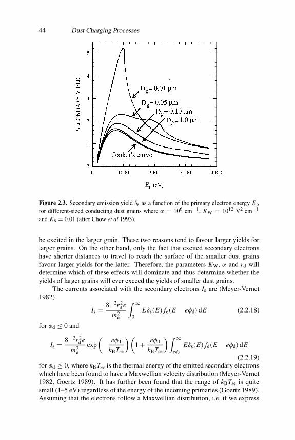
44 Dust Charging Processes
Figure 2.3. Secondary emission yield δs as a function of the primary electron energy Epfor different-sized conducting dust grains where α = 106 cm−1, KW = 1012 V2 cm−1
and Ks = 0.01 (after Chow et al 1993).
be excited in the larger grain. These two reasons tend to favour larger yields forlarger grains. On the other hand, only the fact that excited secondary electronshave shorter distances to travel to reach the surface of the smaller dust grainsfavour larger yields for the latter. Therefore, the parameters KW, α and rd willdetermine which of these effects will dominate and thus determine whether theyields of larger grains will ever exceed the yields of smaller dust grains.
The currents associated with the secondary electrons Is are (Meyer-Vernet1982)
Is = 8π2r2d e
m2e
∫ ∞
0Eδs(E) fe(E − eφd) dE (2.2.18)
for φd ≤ 0 and
Is = 8π2r2d e
m2e
exp
(− eφd
kBTse
)(1+ eφd
kBTse
)∫ ∞
eφd
Eδs(E) fe(E − eφd) dE
(2.2.19)for φd ≥ 0, where kBTse is the thermal energy of the emitted secondary electronswhich have been found to have a Maxwellian velocity distribution (Meyer-Vernet1982, Goertz 1989). It has further been found that the range of kBTse is quitesmall (1–5 eV) regardless of the energy of the incoming primaries (Goertz 1989).Assuming that the electrons follow a Maxwellian distribution, i.e. if we express
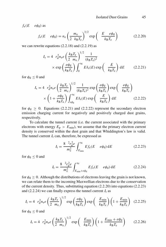
Isolated Dust Grains 45
fe(E − eφd) as
fe(E − eφd) = ne
(me
2πkBTe
)3/2
exp
(− E − eφd
kBTe
)(2.2.20)
we can rewrite equations (2.2.18) and (2.2.19) as
Is = 4πr2d nee
(kBTe
2πme
)1/2 1
(kBTe)2
× exp
(eφd
kBTe
)∫ ∞
0Eδs(E) exp
(− E
kBTe
)dE (2.2.21)
for φd ≤ 0 and
Is = 4πr2d nee
(kBTe
2πme
)1/2 1
(kBTe)2exp
(eφd
kBTe
)exp
(− eφd
kBTe
)
×(
1+ eφd
kBTe
)∫ ∞
eφd
Eδs(E) exp
(− E
kBTe
)dE (2.2.22)
for φd ≥ 0. Equations (2.2.21) and (2.2.22) represent the secondary electronemission charging current for negatively and positively charged dust grains,respectively.
To calculate the tunnel current (i.e. the current associated with the primaryelectrons with energy Ep > Emin), we assume that the primary electron currentdensity is conserved within the dust grain and that Whiddington’s law is valid.The tunnel current It can, therefore, be expressed as
It = 8π2r2d e
m2e
∫ ∞
Emin
E fe(E − eφd) dE (2.2.23)
for φd ≤ 0 and
It = 8π2r2d e
m2e
∫ ∞
Emin+eφd
E fe(E − eφd) dE (2.2.24)
for φd ≥ 0. Although the distributions of electrons leaving the grain is not known,we can relate them to the incoming Maxwellian electrons due to the conservationof the current density. Thus, substituting equation (2.2.20) into equations (2.2.23)and (2.2.24) we can finally express the tunnel current It as
It = 4πr2d nee
(kBTe
2πme
)1/2
exp
(eφd
kBTe
)exp
(− Emin
kBTe
)(1+ Emin
kBTe
)(2.2.25)
for φd ≤ 0 and
It = 4πr2d nee
(kBTe
2πme
)1/2
exp
(− Emin
kBTe
)(1+ Emin + eφd
kBTe
)(2.2.26)

46 Dust Charging Processes
for φd ≥ 0. Chow et al (1993) have numerically analysed the secondary electronemission current given by equations (2.2.21) and (2.2.22) and the tunnel currentgiven by equations (2.2.25) and (2.2.26). They have found that the secondaryelectron current increases with kBTe for kBTe < Em (where Em is the energyof the primary electrons for which the secondary yield δs is maximum) anddominates when kBTe is of the order of Em. It decreases with kBTe whenkBTe � Em. On the other hand, the tunnel current will increase indefinitelywith increasing kBTe and will dominate when kBTe is comparable to or largerthan Emin = (KW Dg)
1/2.
2.2.2.2 Ion impact
The ions approaching a dust grain surface at low kinetic energies (below 1 keV)are neutralized by the electrons which, on the other hand, tunnel through thepotential barrier to neutralize the ions. The energy released in this process mayexcite additional electrons which can then be emitted from the dust grain surface.The number of excited electrons depends on the available potential energy (afterneutralization) which is determined by the ionization potential energy Wi andthe work function Wf of the dust grain material. When a conduction electron iscaptured by the incident ion, it makes available a maximum energy of Wi − Wf.At least Wf of this must be used to free another electron from the material so thatthe condition for the secondary emission is Wi > 2Wf.
When the incident ions have energies above 10 keV, the secondary electronyields due to ion impact can be substantially larger than unity. Draine and Salpeter(1979) showed that the behaviour of such high-energy ions falling on a dustgrain surface may be the same as that of the electrons falling on the dust grainsurface. This means that, like the electrons (incident on a dust grain surface aswe discussed in the previous section), the energetic ions falling on a dust grainmay enter into the dust grain and stop immediately (i.e. stick onto the dust grainsurface) or may pass through the dust material and thus lose their energy (duringtheir passage through the dust grain material), a portion of which can go intoexciting the electrons that in turn may escape from the grain surface. The physicalmodel for the production of the secondary electrons by ion impact (as well asthe dust grain charging currents associated with these secondary electrons andtunnelling ions) is similar to that by electron impact discussed in the previoussection. The sufficiently high-energy ions can also penetrate and re-emit alongwith the secondary electrons. However, the fraction of such re-emitted ionsis usually quite small and thus one can neglect the secondary ion emission incalculating the dust grain surface potential.
2.2.3 Photoemission
When a flux of photons with energy (hν) larger than the photoelectric workfunction (Wf) of the dust grain incidents on the dust grain surface, the latter emits

Isolated Dust Grains 47
photoelectrons, where h is Planck’s constant and ν is the photon frequency. Thephotoemission of electrons depends on (i) the wavelength of the incident photons,(ii) the surface area of the dust grain and (iii) the properties of the dust grainmaterial. This mechanism contributes to a positive charging current and tries tomake the dust grain positively charged. We note that various metals typically havephotoelectric work function Wf < 5 eV, such as Ag (Wf = 4.46 eV), Cu (Wf =4.45 eV), Al (Wf = 4.2 eV), Ca (Wf = 3.2 eV) and Cs (Wf = 1.8 eV). There arealso a number of low work function materials, e.g. carbides (binary compounds ofcarbon and more electropositive metals) with work functions Wf � 2.18–3.50 eV,borides (binary compounds of boron and more electropositive metals) with workfunctions Wf = 2.45–2.92 eV, oxides of metals with work functions ranging fromWf = 1 eV (Cs) to Wf = 4 eV (zirconium).
The maximum charge on a grain, which in the presence of a photon isassumed to emit photoelectrons, can roughly be estimated as follows. We assumethat Wf is the photoelectric work function of the material of the dust grain whichis positively charged (qd > 0). Thus, in order to excite an electron the incomingphotons must have energy hν > Wf + qde/rd. This implies that the maximumdust grain charge is roughly
qd = (hν −Wf)rd
e. (2.2.27)
As the dust grain surface is positive, i.e. φd > 0, a fraction of the photoelectronsreturn to the dust grain surface and the most energetic ones overcome thedust grain potential and escape. Thus, the net current is determined by thebalance between the photoelectrons returned to the dust grain surface and thephotoelectrons escaped from the dust grain surface. The electron photoemissioncurrent for a unidirectional photon flux and for φd > 0 is, therefore, roughly(Rosenberg et al 1996)
Ip = πr2d eJp QabYp exp
(− eφd
kBTp
)(2.2.28)
where Jp is the photon flux, Qab is the efficiency of the absorption for photons(Qab ∼ 1 for 2πrd/λ > 1, where λ is the wavelength of the incident photons),Yp is the yield of the photoelectrons and Tp is their average temperature. It maybe noted that the exponential factor in equation (2.2.28) takes into account thatthe photoelectrons have sufficient energy to overcome the potential barrier of thepositively charged dust grain. It is important to mention that equation (2.2.28)is valid when the photo-emitted electrons follow a Maxwellian distribution withthe temperature Tp. However, in order to take into account the energetics ofthe photoemission processes the assumption of a Maxwellian distribution for thephotoemitted electrons may require some modification.
We now consider a dust grain with negative surface potential. As the dustgrain potential is negative (i.e. φd < 0), no photoelectron returns to the dust grainsurface, i.e. all the photoelectrons emitted by the dust grain surface escape intothe plasma. This leads to a constant current Ip = πr2
d eJp QabYp.

48 Dust Charging Processes
2.2.4 Other charging processes
There are a number of other dust grain charging mechanisms, namely thermionicemission, field emission, radioactivity, impact ionization, etc. These processes,whose importance for a particular application has to be evaluated individually,may be briefly discussed as follows.
2.2.4.1 Thermionic emission
One of the important charging processes which charge up the dust grainspositively is thermionic emission (Sodha and Guha 1971, Rosenberg and Mendis1995). When a dust grain is heated to a high temperature, electrons or ions may bethermionically emitted from the dust grain surface. The thermionic emission maybe induced by laser heating or by thermal infrared (IR) heating or by hot filamentssurrounding the dust grain. The thermionic electron emission current Ith can beobtained from the Richardson equation which, including the increase in the workfunction due to the grain electrostatic barrier, can be expressed as (Rosenberg etal 1999)
Ith = 4πr2d AtT
2d exp
(−|Wf + eφd|
kBTd
)(2.2.29)
where At = 4πemek2B/h3 is a constant.
We now estimate the laser intensity required to heat the dust grains to atemperature Td. We consider an inert gas (e.g. He, Ne, Ar, etc) with disperseddust grains of low work function material and high boiling point. If I is theintensity of the laser energy flux to heat the grains to a temperature Td, the dustgrain heating rate Qheat due to a unidirectional photon flux is
Qheat = πr2d Qab I. (2.2.30)
We consider a gas pressure of about 2 mbar and a grain radius of the order of10 µm, which correspond to typical parameters of dusty plasma experiments.The mean free path of neutrals in the background gas is of the order of 35 µm andthe gas temperature Tn is of the order of 300 K. Thus, in this regime the neutralKnudsen number Kn (the ratio of the neutral mean free path to the grain size) ismuch larger than one. The dust grain loses heat in the gas due to conduction andradiation. The conduction loss rate Qcond in the free molecular regime (Kn � 1)with an accommodation coefficient of the order of unity is
Qcond = πr2d nnVT nkB(Td − Tn) (2.2.31)
where VT n = (kBTn/mn)1/2 is the thermal speed of the background neutral gas.
The blackbody radiative loss rate is
Qrad = πr2d εEσsb(T
4d − T 4
n ) (2.2.32)
Isolated Dust Grains 49
where εE is the emissivity of the grain and σsb is the Stefan–Boltzmann constant.We now consider an example and assume that the dust grains are heated to atemperature of Td � 1700 K and that the temperature and the number densityof the neutral gas (Ne) are Tn � 300 K and nn � 5 × 1016 cm−3, respectively.For this case one can approximate that the radiative loss is about twice as largeas the conductive loss (i.e. Qrad � 2Qcond). Therefore, using equations (2.2.30)–(2.2.32) in Qheat = Qcond + Qrad, the intensity I of the laser energy flux can beapproximated as 300 W cm−2. This intensity can practically be achieved by alow-power IR laser or even perhaps by a series of incandescently hot filamentssurrounding the dust grain.
2.2.4.2 Field emission
There are some special circumstances when micron- or submicron-sized dustgrains may acquire a very high negative (or positive) potential and emit electrons(or ions) as field emission. The onset of electron field emission from a dustgrain surface occurs when its surface electric field is in between 106 V cm−1 and107 V cm−1 (Whipple 1981). The field 106 V cm−1 corresponds to an emissionflux of 105 cm−2 s−1 for a work function of 3.5 eV. As the surface electric field ofa small spherical dust grain is approximately φd/rd, the surface potential φd (involts) corresponding to the surface electric field of 106 V cm−1 is approximately106rd (where rd is in cm). This means that field emission is important for the dustgrains of radii (or the surface with radii of curvature) of the order of a micron. Thedust grain potential is limited by the electron (ion) field emission for negatively(positively) charged dust grains.
2.2.4.3 Radioactivity
Radioactivity in a body in space may constitute a charging mechanism throughboth the escape of the emitted charged primaries from the radioactive nucleiand the escape of the secondary electrons excited by a primary in its passagethrough the surface. The amount of ordinary radioactivity material in bodies isinsignificant for charging effects (Whipple 1981). However, Yanagita (1977)has suggested that the dust grains formed in nova and supernova may havesignificant radioactive levels, particularly Ni22 or Al26 which are β emitters.The charging due to β emission varies with the dimension of the grain andhence larger grains tend to be positively charged. It is also a fact that satellitessometimes carry quantities of radioactive materials in connection with certaintypes of experiments, or as a power source. Though such sources are usuallywell shielded, these may constitute possible charging mechanisms for spacecraft.
2.2.4.4 Impact ionization
When a sufficiently high energetic neutral atom or ion strikes a dust grain surface,either the incident neutral atom or atoms on the grain surface are ionized with
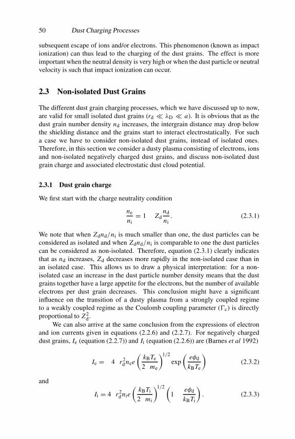
50 Dust Charging Processes
subsequent escape of ions and/or electrons. This phenomenon (known as impactionization) can thus lead to the charging of the dust grains. The effect is moreimportant when the neutral density is very high or when the dust particle or neutralvelocity is such that impact ionization can occur.
2.3 Non-isolated Dust Grains
The different dust grain charging processes, which we have discussed up to now,are valid for small isolated dust grains (rd � λD � a). It is obvious that as thedust grain number density nd increases, the intergrain distance may drop belowthe shielding distance and the grains start to interact electrostatically. For sucha case we have to consider non-isolated dust grains, instead of isolated ones.Therefore, in this section we consider a dusty plasma consisting of electrons, ionsand non-isolated negatively charged dust grains, and discuss non-isolated dustgrain charge and associated electrostatic dust cloud potential.
2.3.1 Dust grain charge
We first start with the charge neutrality condition
ne
ni= 1− Zd
nd
ni. (2.3.1)
We note that when Zdnd/ni is much smaller than one, the dust particles can beconsidered as isolated and when Zdnd/ni is comparable to one the dust particlescan be considered as non-isolated. Therefore, equation (2.3.1) clearly indicatesthat as nd increases, Zd decreases more rapidly in the non-isolated case than inan isolated case. This allows us to draw a physical interpretation: for a non-isolated case an increase in the dust particle number density means that the dustgrains together have a large appetite for the electrons, but the number of availableelectrons per dust grain decreases. This conclusion might have a significantinfluence on the transition of a dusty plasma from a strongly coupled regimeto a weakly coupled regime as the Coulomb coupling parameter (�c) is directlyproportional to Z2
d.We can also arrive at the same conclusion from the expressions of electron
and ion currents given in equations (2.2.6) and (2.2.7). For negatively chargeddust grains, Ie (equation (2.2.7)) and Ii (equation (2.2.6)) are (Barnes et al 1992)
Ie = −4πr2d nee
(kBTe
2πme
)1/2
exp
(eφd
kBTe
)(2.3.2)
and
Ii = 4πr2d nie
(kBTi
2πmi
)1/2 (1− eφd
kBTi
). (2.3.3)

Non-isolated Dust Grains 51
It is obvious that Ii � |Ie| (since me � mi) and the dust grain surface becomesnegatively charged. This increases the ion current and decreases the electroncurrent until Ie + Ii = 0. Using equations (2.3.1)–(2.3.3) in Ie + Ii = 0, wehave (
Time
Temi
)1/2 (1− eφd
kBTi
)exp
(− eφd
kBTe
)= 1− Zd
nd
ni(2.3.4)
where Zd and φd can be related as
φd = − Zde
rd. (2.3.5)
It is clear from equations (2.3.4) and (2.3.5) that for isolated dust grains(Zdnd/ni � 1), φd and Zd depend only on the dust particle radius while fornon-isolated dust grains (Zdnd/ni is comparable to one), φd and Zd do not onlydepend on the dust grain radius, but also on the dust particle number density nd.Now, substituting Zd (obtained from equation (2.3.5)) into equation (2.3.4) andtaking Te = Ti = T we have
1− eφd
kBT−(
mi
me
)1/2 (1+ P
eφd
kBT
)exp
(eφd
kBT
)= 0 (2.3.6)
where P = 4πndrdλ2D0 and λD0 = (kBT/4πnie2)1/2. We can now numerically
solve equation (2.3.6) and can easily calculate φd and Zd. Figure 2.4 shows thevariation of eφd/kBT with log P . When ni, T and rd are assumed to be constant,figure 2.4 shows the effect of nd on φd (or on Zd = −(rd/e)φd). It is obviousfrom figure 2.4 that when we gradually increase nd (i.e. we gradually decreasethe intergrain spacing) and when it exceeds a critical value (i.e. the intergrainspacing becomes smaller than a critical value), the value of −eφd/kBT starts todecrease, i.e. the average dust grain charge Zd starts to decrease. When nd, Tand rd are assumed to be constant, figure 2.4 represents the effect of ni or ne(since ni ∝ ne for a constant nd) on φd (or on Zd) and shows that as we increasethe ambient plasma density (ni or ne), the value of −eφ/kBT increases, i.e. Zdincreases. Furthermore, by plotting curves for different values of rd one can showthat the critical value of nd/ni for which Zd starts to decrease is lower for the dustgrains of larger radii. As an example, in a plasma with a temperature of the orderof 104 K, the charge (Zd) on a 1 µm dust grain starts to be affected by nd/ni whenits value is larger than 3 × 10⁻⁴, while the charge (Zd) on a 0.1 µm dust grainstarts to be affected by nd/ni when its value is larger than 3× 10⁻².
2.3.2 Dust cloud potential
We consider a finite dust cloud immersed in a plasma and follow the modelof Havnes et al (1987) to calculate the dust cloud potential in space plasmas.However, this model may also be applicable for laboratory plasmas in which thetemperatures of the plasma particles (electrons and ions) are not affected by the
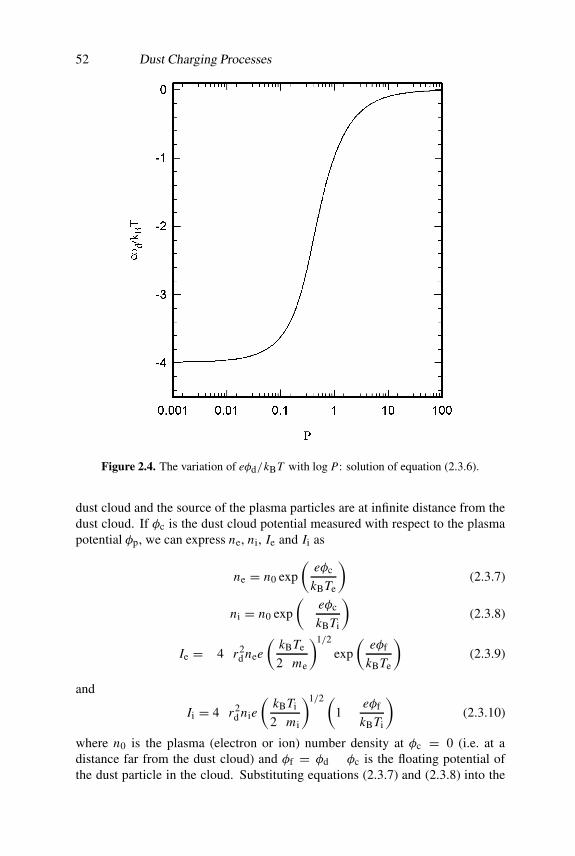
52 Dust Charging Processes
Figure 2.4. The variation of eφd/kBT with log P: solution of equation (2.3.6).
dust cloud and the source of the plasma particles are at infinite distance from thedust cloud. If φc is the dust cloud potential measured with respect to the plasmapotential φp, we can express ne, ni, Ie and Ii as
ne = n0 exp
(eφc
kBTe
)(2.3.7)
ni = n0 exp
(− eφc
kBTi
)(2.3.8)
Ie = −4πr2d nee
(kBTe
2πme
)1/2
exp
(eφf
kBTe
)(2.3.9)
and
Ii = 4πr2d nie
(kBTi
2πmi
)1/2(1− eφf
kBTi
)(2.3.10)
where n0 is the plasma (electron or ion) number density at φc = 0 (i.e. at adistance far from the dust cloud) and φf = φd − φc is the floating potential ofthe dust particle in the cloud. Substituting equations (2.3.7) and (2.3.8) into the
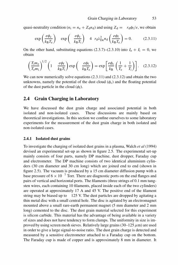
Grain Charging in Laboratory 53
quasi-neutrality condition (ni = ne + Zdnd) and using Zd = −rdφf/e, we obtain
exp
(eφc
kBTe
)− exp
(− eφc
kBTi
)− 4πrdλ
2Dend
(eφf
kBTe
)= 0. (2.3.11)
On the other hand, substituting equations (2.3.7)–(2.3.10) into Ie + Ii = 0, weobtain(
Time
Temi
)1/2 (1− eφf
kBTi
)exp
(− eφf
kBTe
)= exp
[eφc
kB
(1
Te+ 1
Ti
)]. (2.3.12)
We can now numerically solve equations (2.3.11) and (2.3.12) and obtain the twounknowns, namely the potential of the dust cloud (φc) and the floating potentialof the dust particle in the cloud (φf).
2.4 Grain Charging in Laboratory
We have discussed the dust grain charge and associated potential in bothisolated and non-isolated cases. These discussions are mainly based ontheoretical investigations. In this section we confine ourselves to some laboratoryexperiments for the measurement of the dust grain charge in both isolated andnon-isolated cases.
2.4.1 Isolated dust grains
To investigate the charging of isolated dust grains in a plasma, Walch et al (1994)devised an experimental set-up as shown in figure 2.5. The experimental set-upmainly consists of four parts, namely DP machine, dust dropper, Faraday cupand electrometer. The DP machine consists of two identical aluminium cylin-ders (30 cm diameter and 30 cm long) which are joined end to end (shown infigure 2.5). The vacuum is produced by a 15 cm diameter diffusion pump with abase pressure of 6× 10⁻⁷ Torr. There are diagnostic ports on the end flanges andpairs of vertical and horizontal ports. The filaments (three strings of 0.1 mm tung-sten wires, each containing 10 filaments, placed inside each of the two cylinders)are operated at approximately 17 A and 45 V. The positive end of the filamentstring may be biased up to −125 V. The dust particles are dropped by agitating athin metal disc with a small central hole. The disc is agitated by an electromagnetmounted above a small rare-earth permanent magnet (5 mm diameter and 2 mmlong) cemented to the disc. The dust grain material selected for this experimentis silicon carbide. This material has the advantage of being available in a varietyof sizes and does not have tendency to form clumps. The uniformity in size is im-proved by using screen mesh sieves. Relatively large grains (30–125µm) are usedin order to give a large signal-to-noise ratio. The dust grain charge is detected andmeasured by a sensitive electrometer attached to a Faraday cup on the bottom.The Faraday cup is made of copper and is approximately 8 mm in diameter. It

54 Dust Charging Processes
Figure 2.5. Schematic illustration of the DP machine showing the location of the Langmuirprobes, the dust dropper and the Faraday cup (after Walch et al 1994).
is electrostatically shielded and a 6 mm hole in the shield immediately above thecup allows entry of the dust grain. The electrometer is an integrator followed bytwo bandpass amplifiers. The charge falling into the cup is transferred to a 200 pFfeedback capacitor by an operational amplifier to generate a step-wise increase inthe output voltage of the first stage. The voltage is returned to zero by 200 M�
feedback resistor which gives 40 ms decay constant.The grain charge is determined by the floating potential. The net current Inet
isInet = Ie + Ii + If + Is (2.4.1)
where Ie (Ii) is the incident current of the plasma electrons (ions), If is the currentof fast electrons emitted from the filaments and Is is the current of secondaryelectrons emitted from the dust grain due to the fast electron bombardment. It isassumed that photoelectric emission is negligible, because there is little ultravioletradiation in the blackbody spectrum of the filament emission. It is physicallyobvious that each current depends upon the potential of the dust grain as well ason the operating parameters of the experiment. There are two operating regimes,namely the vacuum regime and the plasma regime. The vacuum regime is withoutthe argon gas, i.e. without the plasma (Ie = 0 and Ii = 0). The plasma regime iswith the argon gas, i.e. with the plasma (Ie �= 0 and Ii �= 0).
When there is no plasma (Ie = Ii = 0) and no secondary emission (Is = 0),the dust grains, which should be negatively charged by filament-emitted electron

Grain Charging in Laboratory 55
Figure 2.6. The grain charge as a function of the average grain size at a filament bias of−25 (after Walch et al 1994). These data are for 30–35 µm, 62–74 µm and 95–125 µm.
current If, retard further electrons from the filaments. This occurs when the dustgrain potential is of the order of the potential on the most negative end of thefilament string. The secondary emission can be neglected when the energy ofthe primary electrons is so low that the secondary emission coefficient is small.The dust grain charging time is shorter than the time of flight through the plasma.Walch et al (1994) used 0–125 µm SiC grains and a filament bias of−100 V andshowed that the grain charge is nearly independent of the filament emission foremission currents from 0.25 A to 2 A. It has also been shown by this experimentthat the grain charge begins to decrease when the voltage on the negative end ofthe filament string exceeds 70 V. This indicates that the secondary emission fromSiC grains becomes important for incident electron energies above 70 eV. Thecharging data shown in figure 2.6 are for grains with sizes in the range 30–35µm,62–74 µm and 90–125 µm.
These data are taken for a bias voltage of −25 V where the secondaryemission is unimportant. The charge on the grains increases with size butdeviates from linear scaling. To explain the reason for this deviation, more datacorresponding to the different sizes are needed. When 1 × 10⁻⁴ Torr of argonis added, the plasma is generated in the chamber. The plasma parameters aredetermined from Langmuir probe data. Figure 2.7 shows the probe current–voltage characteristic curve. Typical operating parameters of the DP machine forthe plasma regime are: filament voltage, 45 V; filament current, 17 A; filamentemission current, 1 A; filament bias voltage,−25 V; argon pressure, 1×10⁻⁴ Torr;electron temperature, 2.8 eV; electron density, 6.6 × 108 cm−3; plasma Debyelength, 0.48 cm; plasma potential, 6.8 V; floating potential,−9.0 V.
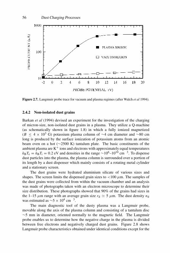
56 Dust Charging Processes
Figure 2.7. Langmuir probe trace for vacuum and plasma regimes (after Walch et al 1994).
2.4.2 Non-isolated dust grains
Barkan et al (1994) devised an experiment for the investigation of the chargingof micron-size, non-isolated dust grains in a plasma. They utilize a Q-machine(as schematically shown in figure 1.8) in which a fully ionized magnetized(B ≤ 4 × 10³ G) potassium plasma column of ∼4 cm diameter and ∼80 cmlong is produced by the surface ionization of potassium atoms from an atomicbeam oven on a hot (∼2500 K) tantalum plate. The basic constituents of theambient plasma are K+ ions and electrons with approximately equal temperatureskBTe = kBTi = 0.2 eV and densities in the range ∼106–1010 cm−3. To dispensedust particles into the plasma, the plasma column is surrounded over a portion ofits length by a dust dispenser which mainly consists of a rotating metal cylinderand a stationary screen.
The dust grains were hydrated aluminium silicate of various sizes andshapes. The screen limits the dispensed grain sizes to <100 µm. The samples ofthe dust grains were collected from within the vacuum chamber and an analysiswas made of photographs taken with an electron microscope to determine theirsize distribution. These photographs showed that 90% of the grains had sizes inthe 1–15 µm range with an average grain size rd � 5 µm. The dust density ndwas estimated as ∼5× 104 cm−3.
The main diagnostic tool of the dusty plasma was a Langmuir probe,movable along the axis of the plasma column and consisting of a tantalum disc∼5 mm in diameter, oriented normally to the magnetic field. The Langmuirprobe enables us to determine how the negative charge in the plasma is dividedbetween free electrons and negatively charged dust grains. Figure 2.8 showsLangmuir probe characteristics obtained under identical conditions except for the
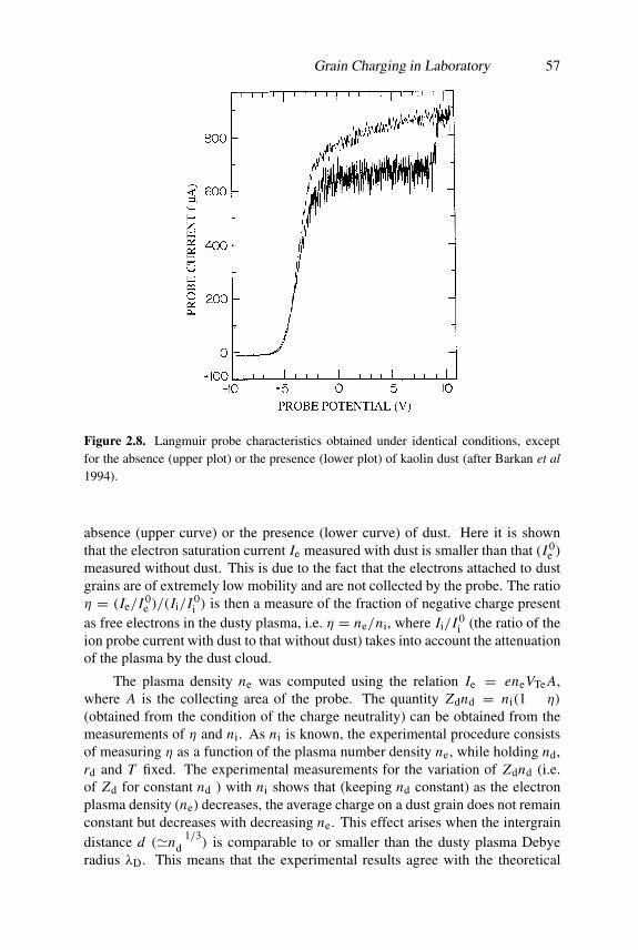
Grain Charging in Laboratory 57
Figure 2.8. Langmuir probe characteristics obtained under identical conditions, exceptfor the absence (upper plot) or the presence (lower plot) of kaolin dust (after Barkan et al1994).
absence (upper curve) or the presence (lower curve) of dust. Here it is shownthat the electron saturation current Ie measured with dust is smaller than that (I 0
e )measured without dust. This is due to the fact that the electrons attached to dustgrains are of extremely low mobility and are not collected by the probe. The ratioη = (Ie/I 0
e )/(Ii/I 0i ) is then a measure of the fraction of negative charge present
as free electrons in the dusty plasma, i.e. η = ne/ni, where Ii/I 0i (the ratio of the
ion probe current with dust to that without dust) takes into account the attenuationof the plasma by the dust cloud.
The plasma density ne was computed using the relation Ie = eneVTe A,where A is the collecting area of the probe. The quantity Zdnd = ni(1 − η)
(obtained from the condition of the charge neutrality) can be obtained from themeasurements of η and ni. As ni is known, the experimental procedure consistsof measuring η as a function of the plasma number density ne, while holding nd,rd and T fixed. The experimental measurements for the variation of Zdnd (i.e.of Zd for constant nd ) with ni shows that (keeping nd constant) as the electronplasma density (ne) decreases, the average charge on a dust grain does not remainconstant but decreases with decreasing ne. This effect arises when the intergraindistance d (�n−1/3
d ) is comparable to or smaller than the dusty plasma Debyeradius λD. This means that the experimental results agree with the theoretical
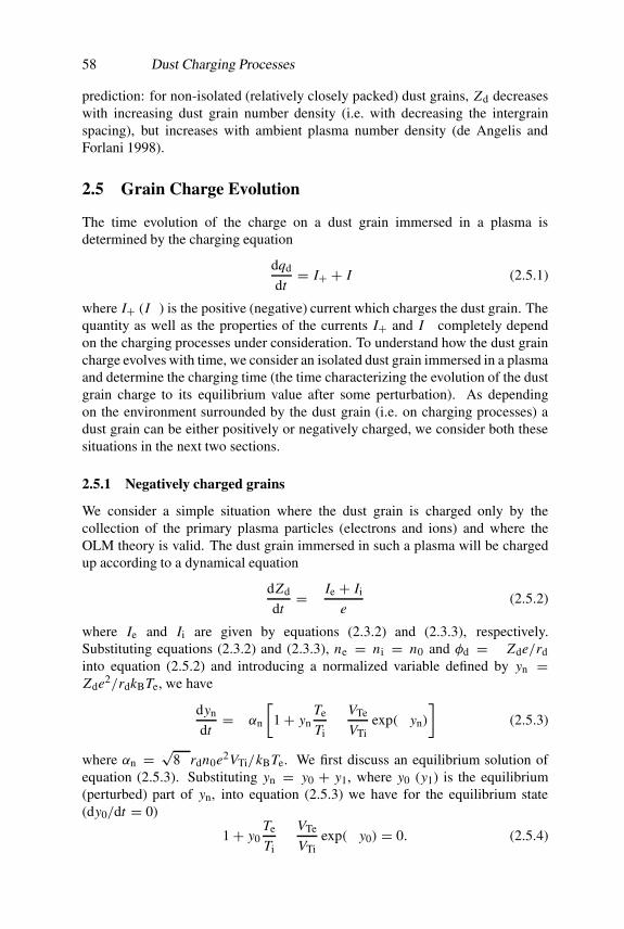
58 Dust Charging Processes
prediction: for non-isolated (relatively closely packed) dust grains, Zd decreaseswith increasing dust grain number density (i.e. with decreasing the intergrainspacing), but increases with ambient plasma number density (de Angelis andForlani 1998).
2.5 Grain Charge Evolution
The time evolution of the charge on a dust grain immersed in a plasma isdetermined by the charging equation
dqd
dt= I+ + I− (2.5.1)
where I+ (I−) is the positive (negative) current which charges the dust grain. Thequantity as well as the properties of the currents I+ and I− completely dependon the charging processes under consideration. To understand how the dust graincharge evolves with time, we consider an isolated dust grain immersed in a plasmaand determine the charging time (the time characterizing the evolution of the dustgrain charge to its equilibrium value after some perturbation). As dependingon the environment surrounded by the dust grain (i.e. on charging processes) adust grain can be either positively or negatively charged, we consider both thesesituations in the next two sections.
2.5.1 Negatively charged grains
We consider a simple situation where the dust grain is charged only by thecollection of the primary plasma particles (electrons and ions) and where theOLM theory is valid. The dust grain immersed in such a plasma will be chargedup according to a dynamical equation
dZd
dt= − Ie + Ii
e(2.5.2)
where Ie and Ii are given by equations (2.3.2) and (2.3.3), respectively.Substituting equations (2.3.2) and (2.3.3), ne = ni = n0 and φd = −Zde/rdinto equation (2.5.2) and introducing a normalized variable defined by yn =Zde2/rdkBTe, we have
dyn
dt= −αn
[1+ yn
Te
Ti− VTe
VTiexp(−yn)
](2.5.3)
where αn =√
8πrdn0e2VTi/kBTe. We first discuss an equilibrium solution ofequation (2.5.3). Substituting yn = y0 + y1, where y0 (y1) is the equilibrium(perturbed) part of yn, into equation (2.5.3) we have for the equilibrium state(dy0/dt = 0)
1+ y0Te
Ti− VTe
VTiexp(−y0) = 0. (2.5.4)

Grain Charge Evolution 59
We can numerically solve equation (2.5.4) for y0 and can easily show that as weincrease Ti/Te (from 0.001 to 0.1), y0 increases (from 0.7 to 2.5). On the otherhand, substituting yn = y0+y1 into equation (2.5.3), we can express the linearizedequation for y1 as
dy1
dt= −αn y1
[Te
Ti+ VTe
VTiexp(−y0)
]. (2.5.5)
Assuming y1 ∝ exp(−t/τc), where τc is the charging time, we can express thecharging time τc (= −y1/(dy1/dt)) as
τc = 1
αn[Te/Ti + (VTe/VTi) exp(−y0)] . (2.5.6)
It is obvious that the charging time τc is a complicated function of Ti or Te, but it isinversely proportional to the plasma density and the dust particle radius. We canalso numerically show that for rd = 0.1 nm, n0 = 5× 109 cm3, Te = 3× 10⁴ Kand Ti = 0.1Te, the charging time τc is of the order of 7 µs.
2.5.2 Positively charged grains
To find the charging time for a positively charged dust grain, we consider asituation where the dust grain is charged by the photoemission of the electrons(in the presence of UV radiation) and the collection of the ions. We also assumethat there are no free ions in the dusty plasma, i.e. all the ions are attached ontothe dust grain surface. The dust grain immersed in such a plasma will be chargedup according to a dynamical equation
dZd
dt= Ie + Ip
e. (2.5.7)
Using equations (2.2.6) and (2.2.28) and φd = Zde/rd the electron collectioncurrent Ie and the photoemission current Ip are
Ie = −πr2d ene
(8kBTe
πme
)1/2(
1+ Zde2
rdkBTe
)(2.5.8)
and
Ip = πr2d eJpYp exp
(− Zde2
rdkBTp
). (2.5.9)
Substituting equations (2.5.8) and (2.4.9) into equation (2.5.7) and introducing anormalized variable defined by zp = Zde2/rdkBTp, we have
dzp
dt= −αp
[1+ zp
Tp
Te− α0 exp(−zp)
](2.5.10)
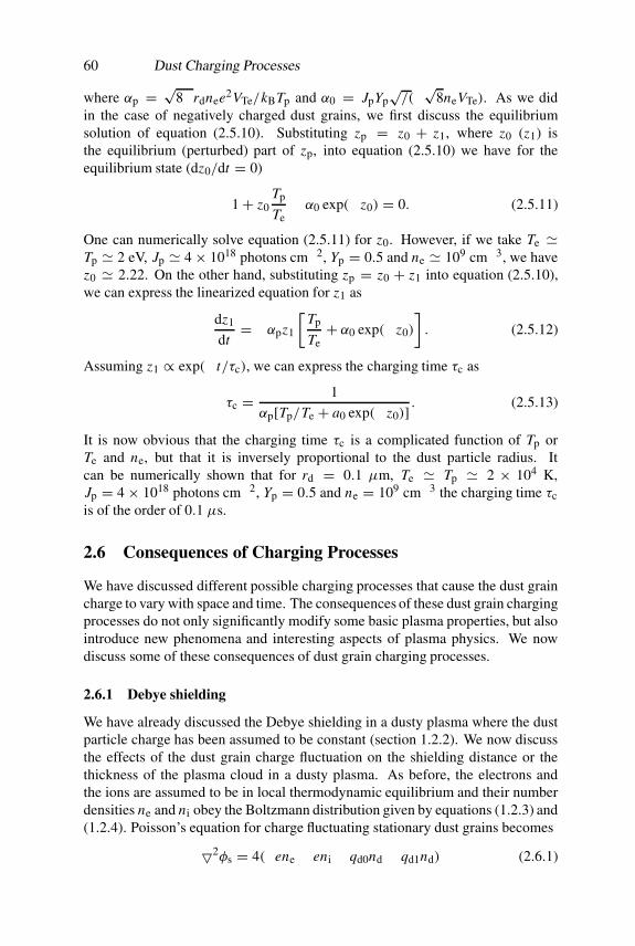
60 Dust Charging Processes
where αp =√
8πrdnee2VTe/kBTp and α0 = JpYp√π/(√
8neVTe). As we didin the case of negatively charged dust grains, we first discuss the equilibriumsolution of equation (2.5.10). Substituting zp = z0 + z1, where z0 (z1) isthe equilibrium (perturbed) part of zp, into equation (2.5.10) we have for theequilibrium state (dz0/dt = 0)
1+ z0Tp
Te− α0 exp(−z0) = 0. (2.5.11)
One can numerically solve equation (2.5.11) for z0. However, if we take Te �Tp � 2 eV, Jp � 4× 10¹⁸ photons cm−2, Yp = 0.5 and ne � 109 cm−3, we havez0 � 2.22. On the other hand, substituting zp = z0 + z1 into equation (2.5.10),we can express the linearized equation for z1 as
dz1
dt= −αpz1
[Tp
Te+ α0 exp(−z0)
]. (2.5.12)
Assuming z1 ∝ exp(−t/τc), we can express the charging time τc as
τc = 1
αp[Tp/Te + a0 exp(−z0)] . (2.5.13)
It is now obvious that the charging time τc is a complicated function of Tp orTe and ne, but that it is inversely proportional to the dust particle radius. Itcan be numerically shown that for rd = 0.1 µm, Te � Tp � 2 × 10⁴ K,Jp = 4× 10¹⁸ photons cm−2, Yp = 0.5 and ne = 109 cm−3 the charging time τcis of the order of 0.1 µs.
2.6 Consequences of Charging Processes
We have discussed different possible charging processes that cause the dust graincharge to vary with space and time. The consequences of these dust grain chargingprocesses do not only significantly modify some basic plasma properties, but alsointroduce new phenomena and interesting aspects of plasma physics. We nowdiscuss some of these consequences of dust grain charging processes.
2.6.1 Debye shielding
We have already discussed the Debye shielding in a dusty plasma where the dustparticle charge has been assumed to be constant (section 1.2.2). We now discussthe effects of the dust grain charge fluctuation on the shielding distance or thethickness of the plasma cloud in a dusty plasma. As before, the electrons andthe ions are assumed to be in local thermodynamic equilibrium and their numberdensities ne and ni obey the Boltzmann distribution given by equations (1.2.3) and(1.2.4). Poisson’s equation for charge fluctuating stationary dust grains becomes
�2φs = 4π(ene − eni − qd0nd − qd1nd) (2.6.1)
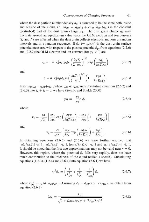
Consequences of Charging Processes 61
where the dust particle number density nd is assumed to be the same both insideand outside of the cloud, i.e. ene0 = qd0nd + eni0, qd0 (qd1) is the constant(perturbed) part of the dust grain charge qd. The dust grain charge qd mayfluctuate around an equilibrium value since the OLM electron and ion currents(Ie and Ii) are affected when the dust grain collects electrons and ions at randomintervals and in a random sequence. If φd (= qd/rd) is the dust grain surfacepotential measured with respect to the plasma potential φp, from equations (2.2.6)and (2.2.7) the OLM electron and ion currents (for qd < 0) are
Ie = −4πr2d ne(φs)e
(kBTe
2πme
)1/2
exp
(eqd
kBTerd
)(2.6.2)
and
Ii = 4πr2d ni(φs)e
(kBTi
2πmi
)1/2 (1− eqd
kBTird
). (2.6.3)
Inserting qd = qd0+qd1, where qd1 � qd0, and substituting equations (2.6.2) and(2.6.3) into Ie + Ii = 0, we have (Stenflo and Shukla 2000)
qd1 = −ν1
ν2rdφs, (2.6.4)
where
ν1 = rd√2π
[ωpe
λDeexp
(eqd0
kBTerd
)+ ωpi
λDi
(1− qd0
kBTird
)](2.6.5)
and
ν2 = rd√2π
[ωpe
λDeexp
(eqd0
kBTerd
)+ ωpi
λDi
]. (2.6.6)
In obtaining equations (2.6.5) and (2.6.6) we have further assumed that|eφs/kBTe| � 1, |eφs/kBTi| � 1, |qd1e/kBTerd| � 1 and |qd1e/kBTird| � 1.It should be noted that the first two approximations may not be valid near r = 0.However, this region, where the potential φs falls very rapidly, does not havemuch contribution to the thickness of the cloud (called a sheath). Substitutingequations (1.2.3), (1.2.4) and (2.6.4) into equation (2.6.1) we have
�2φs =(
1
λ2De
+ 1
λ2Di
+ 1
λ2Dg
)φs (2.6.7)
where λ−2Dg = ν2/4πnd0rdν1. Assuming φs = φs0 exp(−r/λDc), we obtain from
equation (2.6.7)
λDc = λDi√1+ (λDi/λDe)2 + (λDg/λDi)2
(2.6.8)

62 Dust Charging Processes
which is a measure of the shielding distance or the thickness of the sheath ina dusty plasma with the charge fluctuating dust grains. The term (λDg/λDi)
2
represents the effect of the dust grain charge fluctuation. For a dusty plasma withnegatively charged dust particles we have ne0 � ni0 and Te ≥ Ti, i.e. λDe � λDi.Thus, equation (2.6.8) reduces to
λDc � λDi√1+ (λDg/λDi)2
. (2.6.9)
Equation (2.6.9) clearly explains how the Debye length is modified by the dustgrain charge fluctuation. It is obvious that when the dust grain radius is verysmall, i.e. when λDg � λDi, one can neglect the effect of this dust grain chargefluctuation. However, when λDg is comparable to λDi, one should take intoaccount the effect of dust grain charge fluctuations.
2.6.2 Electrostatic sheath
We have discussed the properties of the electrostatic sheath in a dusty plasma withconstant charged dust particles (section 1.5). We now wish to explain the effect ofthe dust grain charge fluctuation on some basic properties of such an electrostaticsheath. We consider almost the same dusty plasma model as we considered insection 1.5. The only difference is that instead of a constant dust grain charge wewill consider here a fluctuating dust grain charge. Thus, as before the electronnumber density ne is given by equation (1.2.3) and the ion number density ni isgiven by (1.6.5). Using equations (1.2.3), (1.6.5) and qd0nd0 = ene0 − eni0 wecan express Poisson’s equation in terms of normalized variables as
d2ψs
dξ2= δ
(1+ 2ψs
M2
)−1/2
− exp(−ψs)− (δ − 1)Qd
Qd0(2.6.10)
where Qd = eqd/kBTerd and Qd0 = eqd0/kBTerd. We note that for constantcharged dust particles, Qd/Qd0 = 1 and equation (2.6.10) is identical withequation (1.6.5). But for the present case the charge Qd is not constant and isdetermined from the condition Ie + Ii = 0, where Ie is given by equation (2.6.2)and Ii is
Ii = πr2d enivi
(1− 2eqd
rdmiv2i
). (2.6.11)
Using equations (1.2.3), (1.2.4), (2.6.2) and (2.6.11) we can express the conditionIe + Ii = 0 in the form
(πme
8mi
)1/2
δM(M2 − 2Q′d)e−Q ′d = M2 + 2ψs (2.6.12)
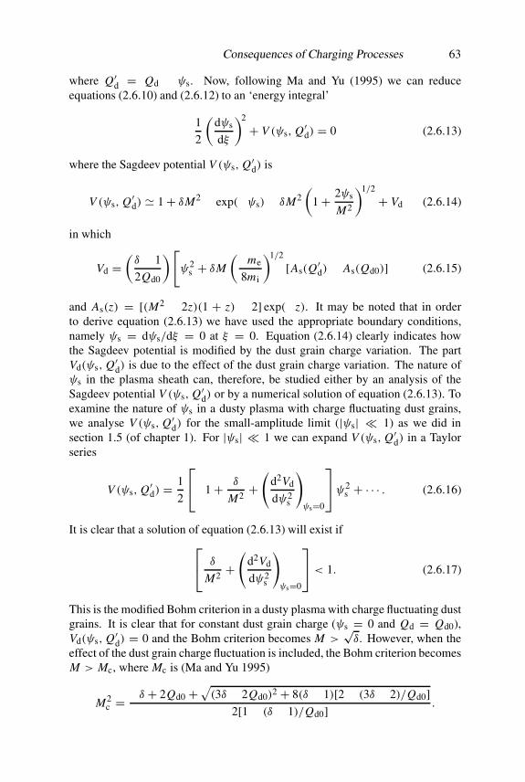
Consequences of Charging Processes 63
where Q′d = Qd − ψs. Now, following Ma and Yu (1995) we can reduceequations (2.6.10) and (2.6.12) to an ‘energy integral’
1
2
(dψs
dξ
)2
+ V (ψs, Q′d) = 0 (2.6.13)
where the Sagdeev potential V (ψs, Q′d) is
V (ψs, Q′d) � 1+ δM2 − exp(−ψs)− δM2(
1+ 2ψs
M2
)1/2
+ Vd (2.6.14)
in which
Vd =(δ − 1
2Qd0
)[ψ2
s + δM
(πme
8mi
)1/2
[As(Q′d)− As(Qd0)]
](2.6.15)
and As(z) = [(M2 − 2z)(1 + z) − 2] exp(−z). It may be noted that in orderto derive equation (2.6.13) we have used the appropriate boundary conditions,namely ψs = dψs/dξ = 0 at ξ = 0. Equation (2.6.14) clearly indicates howthe Sagdeev potential is modified by the dust grain charge variation. The partVd(ψs, Q′d) is due to the effect of the dust grain charge variation. The nature ofψs in the plasma sheath can, therefore, be studied either by an analysis of theSagdeev potential V (ψs, Q′d) or by a numerical solution of equation (2.6.13). Toexamine the nature of ψs in a dusty plasma with charge fluctuating dust grains,we analyse V (ψs, Q′d) for the small-amplitude limit (|ψs| � 1) as we did insection 1.5 (of chapter 1). For |ψs| � 1 we can expand V (ψs, Q′d) in a Taylorseries
V (ψs, Q′d) =1
2
−1+ δ
M2+(
d2Vd
dψ2s
)ψs=0
ψ2
s + · · · . (2.6.16)
It is clear that a solution of equation (2.6.13) will exist if δ
M2+(
d2Vd
dψ2s
)ψs=0
< 1. (2.6.17)
This is the modified Bohm criterion in a dusty plasma with charge fluctuating dustgrains. It is clear that for constant dust grain charge (ψs = 0 and Qd = Qd0),Vd(ψs, Q′d) = 0 and the Bohm criterion becomes M >
√δ. However, when the
effect of the dust grain charge fluctuation is included, the Bohm criterion becomesM > Mc, where Mc is (Ma and Yu 1995)
M2c =
−δ + 2Qd0 +√(3δ − 2Qd0)2 + 8(δ − 1)[2− (3δ − 2)/Qd0]
2[1− (δ − 1)/Qd0] .

64 Dust Charging Processes
Figure 2.9. The variation of the critical Mach number Mc with δ.
This clearly explains how the effect of the dust grain charge fluctuation modifiesthe Bohm criterion or the critical Mach number Mc. Since δ is a function of nd0,the Bohm criterion or the critical Mach number is significantly modified by thedust particle number density as well by the dust grain charge at x = 0. A plot ofMc versus δ, as shown in figure 2.9, indicates that Mc increases with δ for valueswithin a smaller range. This means that a larger accelerating field is required forpushing the ions towards the wall. Figure 2.9 also shows that Mc decreases withδ for its values within a higher range. This means that for higher values of δ theelectrons become virtually depleted, so that the dust grains are less negative andMc can be smaller.
2.6.3 Coagulation of dust grains
It is well known that in the secondary emission the current–energy curve can havemultiple roots. This fact led Meyer-Vernet (1982) to propose that dust grainswith identical electrical properties, embedded in the same plasma but havingdifferent charging histories, could achieve opposite potentials. This idea wasfurther developed by Horanyi and Goertz (1990). The variation of the normalizedgrain surface potential (eφd/kBT ) as a function of the plasma temperature (Te =Ti = T ) for different values of the secondary yield parameter (δm) is shown infigure 2.10. As an illustration, we consider grains of different sizes immersed ina plasma and assume that they all have the same δm = 8. We suppose that thetemperature of the plasma is gradually increased. The potentials of all the grainswill follow the δm = 8 curve. At a lower plasma temperature T < T1, the grainsurface potential is negative because the flux of the secondary electron emissionis smaller than that of the primary electrons. At a higher temperature T > T2,
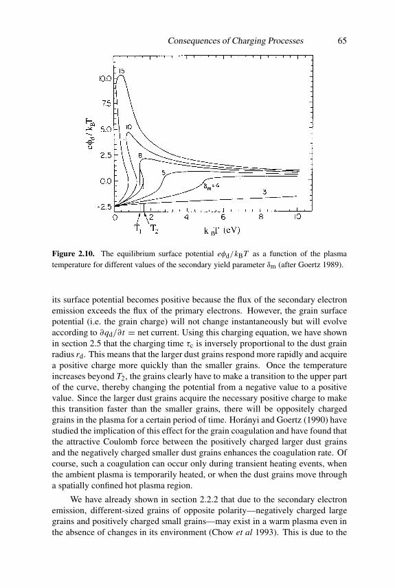
Consequences of Charging Processes 65
Figure 2.10. The equilibrium surface potential eφd/kBT as a function of the plasmatemperature for different values of the secondary yield parameter δm (after Goertz 1989).
its surface potential becomes positive because the flux of the secondary electronemission exceeds the flux of the primary electrons. However, the grain surfacepotential (i.e. the grain charge) will not change instantaneously but will evolveaccording to ∂qd/∂ t = net current. Using this charging equation, we have shownin section 2.5 that the charging time τc is inversely proportional to the dust grainradius rd. This means that the larger dust grains respond more rapidly and acquirea positive charge more quickly than the smaller grains. Once the temperatureincreases beyond T2, the grains clearly have to make a transition to the upper partof the curve, thereby changing the potential from a negative value to a positivevalue. Since the larger dust grains acquire the necessary positive charge to makethis transition faster than the smaller grains, there will be oppositely chargedgrains in the plasma for a certain period of time. Horanyi and Goertz (1990) havestudied the implication of this effect for the grain coagulation and have found thatthe attractive Coulomb force between the positively charged larger dust grainsand the negatively charged smaller dust grains enhances the coagulation rate. Ofcourse, such a coagulation can occur only during transient heating events, whenthe ambient plasma is temporarily heated, or when the dust grains move througha spatially confined hot plasma region.
We have already shown in section 2.2.2 that due to the secondary electronemission, different-sized grains of opposite polarity—negatively charged largegrains and positively charged small grains—may exist in a warm plasma even inthe absence of changes in its environment (Chow et al 1993). This is due to the

66 Dust Charging Processes
fact that the excited secondary electrons have shorter distances to travel to reachthe surface of the smaller dust grains.
Chow et al (1993) have also calculated the equilibrium potential forinsulating grains immersed in both Maxwellian and generalized Lorentzianplasmas. Due to the size effect on the secondary emission they have foundthat insulating grains with diameters 0.01 µm and 1 µm have opposite polarity(with smaller ones being positive) when the plasma temperature is in the range25–48 eV for a Maxwellian plasma and in the range 7–17 eV for a Lorentzianplasma (κ = 2). These values may be in the range of the inferred values ofkBTe in different regions of planetary ring systems, comets, the interplanetarymedium, supernova remnants, etc (Goertz 1989, Mendis and Horanyi 1991,Mendis and Rosenberg 1994). Therefore, the existence of different-sized grainsof opposite polarity (negatively charged large grains and positively charged smallgrains) is possible, i.e. enhanced coagulation may also take place in all of theseenvironments.
It has been shown by Feuerbacher et al (1973) that the photoemission maycause the dust grains to acquire opposite charges in the same plasma and radiativeenvironment, even if they have the same size, provided that they have wildlydifferent photoemission yields. This also can lead to an enhanced dust coagulationin certain regions of interstellar space.
2.6.4 Disruption of dust grains
Coagulation is not the only physical effect of grain charging. The exactly oppositeeffect, namely physical disruption of the dust grains, could also occur if the grainsacquire a very high potential. This is a consequence of the electrostatic repulsionof like surface charges, which produces electrostatic tension in the body. If theelectrostatic tension exceeds the tensile strength of the body across any section,the body will break up across that section. Opik (1956) showed that electrostaticdisruption will occur across a section if the electrostatic energy density (φ2
g/8πr2d )
exceeds the tensile strength Ft, i.e.
Ft <φ2
g
8πr2d
. (2.6.18)
We can express this in a way that the electrostatic disruption will occur if the grainradius is less than a critical value r c
d, i.e.
rd < r cd = 6.65F−1/2
t |φg| (2.6.19)
where φg is in volts, Ft is in dyn cm−2 and r cd (or rd) is in microns. It is clear from
equation (2.6.19) that as the size of the dust grains (i.e. rd) decreases, the valueof Ft required to prevent grain disruption increases rapidly. This also impliesthat as a dust grain begins to disrupt electrostatically, the process continues untilsmaller fragments for which rd > r c
d appear. If this were so, it also provides

Consequences of Charging Processes 67
an insurmountable obstacle for the growth of the dust grain in a plasma. Whatthe dust grain enables to circumvent this runaway disruption is the electric fieldemission of the electrons from small grains (Mendis 1991). This is because as thegrain radius decreases, the surface electric field increases to reach such a value(typically �107 V cm−1) that rapid electron emission occurs from negativelycharged dust grains and the value of the grain potential decreases to a valuethat is no longer given by the plasma environment but rather by the size alone,e.g. φg � 900rd (Mendis and Rosenberg 1994). Substituting φg � 900rd intoequation (2.6.19) we find that when Ft > 3.6 × 10⁷ dyn/cm2, the electric fieldemission limitation of the grain potential will prevent electrostatic disruptionof the grains, regardless of their size. Consequently, materials such as iron(Ft � 2× 10¹⁰ dyn cm−2) and tektites (Ft � 7 × 10¹⁰ dyn cm−2) are stabilizedby this process against electrostatic disruption no matter how small the size is. Onthe other hand, very fragile grains such as cometary grains (Ft � 106 dyn cm−2)of very small radii (�A) will be stable only if φd ≤ 0.15 eV. It is importantto note that the electric field emission effect will enable the growth of the dustgrain to take place in the above environments only if the grains are negativelycharged. This means that if there is sufficient UV radiation to make the graincharge positive due to the photoemission, the growth of the dust grains will notproceed even in a low-temperature plasma.
2.6.5 Disruption of bacteria
Recently, Mendis et al (2000) have modelled an electro-physical mechanism forthe electrostatic disruption of a bacterium in the discharge plasma (Laroussi et al1999). They have shown that the electrostatic disruption of the bacterium takesplace when the bacterium has acquired a sufficient electrostatic charge for whichthe outward electrostatic stress exceeds its tensile strength. It also appears intheir model that surface roughness or irregularity would render it more sensitiveto electrostatic disruption. To illustrate this model, we idealize the bacterium tobe a sphere of radius Rb, with a hemispherical irregularity (a ‘pimple’) of radiusrb � Rb. We also assume the outer membrane to have a thickness �b (�rb, Rb)and to have a uniform surface potential φb. Since the electrostatic disruptionwill take place across a section with minimum radius of curvature because of thelarger electric fields there (Hill and Mendis 1981b), in this case the condition forthe electrostatic disruption is that the component of the total electric force alongthe axis joining the centres of the larger spheres and small hemisphere exceedsthe total tensile force on the membrane along this axis, i.e.
∫ rb
0
(φ2
b
8πr2b
)2πρ dρ > Ft · 2π rb�b (2.6.20)
where ρ is the cylindrical coordinate normal to this axis, Ft is the tensile strengthof the membrane and φ2
b/8π is the electrostatic tension normal to the surface of
68 Dust Charging Processes
the bacterium. If we express Ft in dyn cm−2, φb in volts, and rb, Rb and �b inµm, equation (2.6.20) leads to the condition
|φb| ≥ 0.2(rb�b Ft)1/2. (2.6.21)
We note that if the bacterium had been idealized as a perfect sphere, thecondition for disruption across the middle (into two hemispheres) is obtainedfrom equation (2.6.21) by replacing rb by Rb. So, it is easier to disrupt or tearthe membrane by breaking off the ‘pimple’ than by breaking it into more or lessequal pieces.
To have some numerical appreciations of the analytical results, let us takeRb = 1 µm, �b = 0.008 µm (Madigan et al 1997) and rb = 0.02 µm. Theactual measured value of the tensile strength Ft of the outer membrane is notavailable. However, since Gram-negative bacteria can maintain turgor pressureof 1–5 atm and the purpose of the strong murein layer appears to withstandsuch pressures (Madigan et al 1997), it seems that the tensile strength of themembranes (both inner and outer) could not exceed the above values. We,therefore, assume that Ft = (1–5) × 106 dyn cm−2. If we assume the highervalue, i.e. Ft = 5 × 10⁶ dyn cm−2, we obtain |φb| ≥ 6 V as the conditionfor the electrostatic disruption of the membrane by rupturing the pimple. Thecondition to break it in half (obtained by replacing rb by Rb in equation (2.6.21)) is|φb| ≥ 40 V. If we use the smaller value of Ft (∼106 dyn cm−2) the correspondingconditions are, respectively, |φb| ≥ 3 V and |φb| ≥ 18 V.
On the other hand, in a glow discharge plasma experiment of Laroussi et al(1999), the plasma electron temperature kBTe = 1–5 eV. If we assume that bothelectrons and ions (largely He+) are Maxwellian with Te = Ti (although Te issignificantly larger than Ti in this case), and solve the standard transcendentalequation for the equilibrium potential obtained by equating the orbit-limitedelectron and ion currents to the bacterium immersed in the plasma, we obtain(Mendis et al 2000) |φb| � 15 V if kBTe = 5 eV. In such discharges, the plasmas(particularly, the electrons) are not expected to be Maxwellian, having thickertails at higher energies and are better fit by generalized Lorentzian κ-distribution(Rosenberg and Mendis 1992). If we assume this to be the case with κ = 2, weget |φb| � 20 V. We, therefore, see that the potential expected to be achieved bythe E. coli bacteria in a glow discharge plasma could be sufficient to break theouter membrane in half if its tensile strength is low (Ft � 106 dyn cm−2). If thetensile strength is higher (Ft � 5× 10⁶ dyn cm−2), the surface potential achievedis insufficient to break this membrane in half, but would be sufficient to tear it ifit had a surface roughness on the scale of a few percent (Mendis et al 2000).
2.6.6 Levitation of dust grains
The electrostatic charging of the dust grains can also lead to the levitation ofthe fine dust lying on large surfaces. In this case, the charge qd acquired by thedust grain is proportional to its projected surface area (Mendis and Rosenberg

Consequences of Charging Processes 69
1994) and so qd = surface area× surface charge density = (1/4)(rd/λD)(rdφd).Typically rd/λD � 1 and hence the dust grain charge in a plasma medium ismuch smaller than that in free space. Mendis et al (1982) considered the chargingof the bare cometary nucleus by the solar wind plasma and the solar UV radiationat large heliocentric distances. They showed that while the subsolar point of thecometary surface acquires a positive potential of the order of 15 V due to thedominance of the photoemission, the nightside could acquire a negative potentialof the order of−1 kV (where the solar wind speed is considered to be of the orderof 600 km s−1). Consequently, submicron-sized dust grains could overcome thegravitational attraction of the nucleus and levitate on the nightside of the comet,even when they had a deficit of just one electron charge.
Chapter 3
Dynamics of Dust Grains
3.1 Introduction
The dynamics of charged dust grains in space attracted the main stream of interestof space physicists about 20 years ago, when Voyager 1 and 2 passed Saturnand sent back pictures of mysterious dark spokes sweeping around the B ring(Smith et al 1981, 1982). It was then independently proposed by Hill and Mendis(1981a) and Goertz and Morfill (1983) that the spokes might be charged dustand sculptured by electrostatic forces. The dynamical patterns of charged dustparticles in interplanetary space observed by Voyager 1 and 2 also seem to accountfor the combined effects of electromagnetic and gravitational forces acting on thedust particles. On the other hand, in laboratory plasmas, dust particles, which aresubjected to various forces, often accumulate near the plasma boundaries (walls)and cause contamination to substrates and wafers (Selwyn 1993). It is, therefore,crucial to understand the behaviour of macroscopic particles under the action ofvarious forces (such as gravitational force, electric force, ion drag force, neutraldrag force, thermophoretic force, etc) in order to control the dust transport. Thus,in this chapter, we confine ourselves to the study of different forces acting oncharged dust particles and their dynamics in both space and laboratory dustyplasmas. The forces that are relevant to dust grain crystallization are discussedin chapter 8.
3.2 Forces on Dust Grains
There are a number of forces, such as electromagnetic force, gravitational force,ion and neutral drag forces, thermophoretic force, radiation pressure force, etcthat may act on charged dust grains and may govern their dynamics in the plasma.The basic equation governing the dynamics of a charged dust grain of mass mdand velocity vd is
mddvd
dt= FEL + FG + FD + FT + FP (3.2.1)
70

Forces on Dust Grains 71
where FEL is the electromagnetic force associated with the combined effects ofthe electric and magnetic fields, FG is the gravitational force associated with theattraction between the dust particles themselves (if they are massive enough) orbetween the dust particle and the massive planet or satellite, FD is the drag forceassociated with the dragging of plasma particles or neutrals, which in fact arisesfrom the relative motion between the plasma and the dust, or between the neutraland the dust, FT is the thermophoretic force associated with the temperaturegradient of the neutral gas and FP is the radiation pressure force.
3.2.1 Electromagnetic force
The electromagnetic force FEL acting on a moving charged dust particle of chargeqd is the sum of the electric force
FE = qd E (3.2.2)
and the Lorentz forceFL = qd
cvd × B (3.2.3)
where E is the electric field and B is the magnetic field. That is, we have
FEL = FE + FL = qd
(E + 1
cvd × B
). (3.2.4)
We consider this force first in space dusty plasmas and later in laboratory dustyplasmas.
We consider a magnetized planet in which the magnetic field B can befurther simplified by assuming that it is the field of a magnetic dipole of momentM located at its (planet’s) centre of gravity and oriented along its rotation axis.Thus, we can express B(r) as
B(r) = 3r(M r)r−5 − Mr−3 (3.2.5)
where r is the distance from the centre of gravity of the planet. Within theequatorial plane, equation (3.2.5) becomes
B(r) = −Mr−3 (3.2.6)
and|B(r)| = B0L−3 (3.2.7)
where B0 is the magnitude of the magnetic field at the planet surface and L (=r/Rp, where Rp is the planet radius) is the magnetic shell parameter. We assumethat the planet is a uniformly magnetized sphere. The induction B(r) and the fieldstrength H(r) are equal at any point outside the planet, but are different inside theplanet due to the magnetization. Therefore, inside the planet we can express B(r)and H(r) as
B(r ≤ Rp) = 2M R−3p (3.2.8)

72 Dynamics of Dust Grains
Table 3.1. Typical magnetic field parameters of Earth, Saturn and Jupiter.
Parameter Earth Saturn Jupiter
M (G cm3) 8× 1025 4.4× 1028 1.6× 1030
B0 (G) 0.5 0.2 4.2Rp (cm) 6.38× 10⁸ 6.03× 10⁹ 7.14× 10⁹
andH(r ≤ Rp) = −M R−3
p . (3.2.9)
The magnetic field parameters of different planets, namely Earth, Saturn andJupiter are given in table 3.1. The electric field E near a rotating magnetizedsphere can be evaluated in a simple way by assuming that the plasma isof sufficiently high conductivity (i.e. σcon → ∞, where σcon is the plasmaconductivity) and co-rotates rigidly with the angular rotation frequency �pl ofthe magnetized planet. The medium would be at rest in a moving frame movingat the velocity Vpl = �pl× r with respect to the fixed point of observation. Thus,we can express Ohm’s law in the form
j = σcon
(E + 1
cVpl × B
)(3.2.10)
where j is the current density observed in the fixed frame (transformation of thevalue j itself results in corrections of the order V 2
pl/c2 that are neglected). Theassumption that the current density j is finite at σcon → ∞ allows us to expressthe electric field as
E = −1
c[(�pl × r)× B]. (3.2.11)
The force FEL acting on a dust particle orbiting the planet at an angular velocityωd (i.e. with the velocity vd = ωd × r) is (Bliokh et al 1995)
FEL = qd
c{[(ωd −�pl)× r] × B}. (3.2.12)
We consider the force FEL acting on a dust particle within the equatorial plane,where FEL is radially oriented and B = B0/L3. Thus, within the equatorialplane, we have FEL = (qd B0r/L3c)(ωd − �pl). This means that the Lorentzforce is zero at the synchronous orbit where ωd = �pl. It is important to notehere that equation (3.2.12) is valid for a highly conducting plasma around theplanet. However, it is also possible to analyse the unipolar induction E withoutconsidering this assumption.
We now consider electric forces in a laboratory dusty plasma in which themagnetic force is almost insignificant. We particularly concentrate on the electric

Forces on Dust Grains 73
force that a conducting (i.e. equipotential) dust particle in a plasma in the presenceof a non-zero macroscopic field (i.e. a pre-sheath field of a glow discharge)experiences. To calculate such an electric force acting on a dust particle, we startwith the linearized Poisson equation (1.2.6) that can be expressed in sphericalcoordinates with an azimuthal symmetry as
1
r2
∂
∂r
(r2 ∂φs
∂r
)+ 1
r2 sin θ
∂
∂θ
(sin θ
∂φs
∂θ
)= k2
Dφs (3.2.13)
where k2D = λ−2
De + λ−2Di . The boundary condition far from the particle is now a
constant field condition, which in spherical coordinates takes the form
φs(r, θ)|r→∞ = −E0r cos θ (3.2.14)
where E0 is the constant electric field strength. The surface of a conducting dustparticle is at a uniform potential φd. Thus, the boundary condition at the particlesurface is
φs(r, θ)|r→rd = φd. (3.2.15)
Also, all the components of ∇φs tangential to the surface of the dust grain, whichis assumed to be a conductor, vanish, i.e.
(∇φs)θ |r→rd = 0. (3.2.16)
Introducing the variable transformations ξ = kDr and µ = cos θ we can expressequation (3.2.13) in the form
1
ξ2
∂
∂ξ
(ξ2 ∂φs
∂ξ
)+ 1
ξ2
∂
∂µ
[(1− µ2)
∂φs
∂µ
]= φs. (3.2.17)
Substitutingφs(ξ, µ) = Y (ξ)Z(µ) (3.2.18)
into equation (3.2.17), we can separate the latter into two ordinary differentialequations, namely
ξ2 d2Y
dξ2 + 2ξdY
dξ− [ξ2 + n(n + 1)]Y = 0 (3.2.19)
and
(1− µ2)d2 Z
dµ2− 2µ
dZ
dµ+ n(n + 1)Z = 0 (3.2.20)
where n = 0, 1, 2, . . . . It is obvious that the modified spherical Bessel functionsand Legendre functions are the solutions of equations (3.2.19) and (3.2.20),respectively. Therefore, substituting these two solutions into equation (3.2.18)we have (Daugherty et al 1993)
φs(ξ, µ) = φ∞ + A0
(1
ξ
)exp(−ξ)+ A1µ
(1
ξ+ 1
ξ2
)exp(−ξ)+ · · · (3.2.21)
74 Dynamics of Dust Grains
where φ∞, A0 and A1 are constants. The latter can be determined by the boundaryconditions given in equations (3.2.14)–(3.2.16), i.e. equation (3.2.14) determinesφ∞ = −E0r cos θ , equation (3.2.15) determines A0 = φdkDrd exp(kDrd) andequation (3.2.16) determines A1 = [E0k2
Dr3d/(1 + kDrd)] exp(kDrd). All other
higher-order terms vanish for a constant field boundary condition, i.e. terms withcos2 θ and higher are not needed to match a constant field condition. Therefore,the solution of equation (3.2.13) for the perturbed potential profile is
φs(r, θ) = − E0r cos θ + φdrd
rexp[−kD(r − rd)]
+ E0k2Dr3
d
1+ kDrdcos θ
(1
kDr+ 1
k2Dr2
)exp[−kD(r − rd)]. (3.2.22)
It is obvious from equation (3.2.22) that the electric potential φs(r, θ) consists ofthree separate potential fields. The first term is the potential due to the constantapplied field E0. The second term is the spherically symmetric Debye–Huckelpotential. The last term is the polarization response of the plasma, and it dependson cos θ and represents the characteristics of a dipole distribution of the dust graincharge.
The electrostatic force associated with this potential field may be calculatedby the application of the electrostatic stress tensor (Daugherty et al 1993). Theelectrostatic force FE on the spherical dust grain is given by
FE = 1
4π
∮surface
[Es(Es · n)− 1
2E2
s n]
dA (3.2.23)
where E2s is the square of the magnitude of the surface electric field vector.
We have considered the dust grain as a conducting sphere, i.e. the electric fieldis normal to its surface. Therefore, for spherical symmetry we can simplifyequation (3.2.23) as
FEz = 1
4r2
d
∫ π
0
[(∂φs
∂r
)r=rd
]2
cos θ sin θ dθ. (3.2.24)
Note that the constant electric field E0 is along the z-direction. Substitutingequation (3.2.22) into equation (3.2.24) and then performing the integration wehave
FEz = rdφd E0(1+ kdrd)
[1+ k2
Dr2d
3(1+ kDrd)
]. (3.2.25)
Equation (3.2.25) can be further simplified by calculating φd in terms of the dustgrain charge
qd = 2πr2d
∫ π
0σq(θ) sin θ dθ (3.2.26)

Forces on Dust Grains 75
where the surface charge density σq(θ) is given by
σq(θ) = − 1
4π
(∂φs
∂r
)r=rd
. (3.2.27)
Using equations (3.2.22), (3.2.26) and (3.2.27) we can express qd as
qd = rdφd(1+ kdrd). (3.2.28)
Substituting φd (obtained from (3.2.28)) into equation (2.3.25) we finally obtain
FEz = qd E0
[1+ k2
Dr2d
3(1+ kDrd)
]. (3.2.29)
Equation (3.2.29) implies that for most of the dusty plasma in which kDrd � 1,we have FEz � qd E0. It also implies an intersecting result that the plasma doesnot shield the dust particle from the bulk electric field and thereby the electrostaticforce is reduced. This prediction was first made by Daugherty et al (1993) by theiranalytical calculations of electrostatic forces acting on small particles in a uniformplasma in the presence of a constant electric field E0. However, there are somesituations where the electric field may be associated with a non-uniform plasmadensity and where the deformation of the sheath may occur due to the densitygradient.
Hamaguchi and Farouki (1994) have investigated the electrostatic forceacting on a dust particle in a plasma in the presence of a density gradient andan externally applied constant electric field E0. They have shown that anotherforce, which is proportional to the density gradient (or the Debye-length gradient)should be added in order to account for the deformation of the sheath. Theyderived a first-order correction to the Debye–Huckel potential associated withthe density or Debye-length gradient by expanding the linearized Debye lengtharound the position of the dust grain. They have expressed the total force actingon a dust particle as
FEz = qd E0 − q2d
2(λD + rd)2
(dλD
dz
)(3.2.30)
where λD = 1/kD. The total force is clearly the superposition of two separateforces. The first term is the electric force which is due to the constant applied dcelectric field E0 and is unaffected by the sheath, as predicted by Daugherty et al(1993). The second term is another force known as polarization force which isdue to the gradient in the density.
3.2.2 Gravitational force
The gravitational force FG acting on a dust particle is in general a combination(resultant) of three forces, namely (i) the force of attraction acting on a dust grain

76 Dynamics of Dust Grains
by the nearby planet: FGp = GmdMp r/r3, where G = 6.672×10⁻⁸ dyn cm2 g−2
is the gravitational constant and r is the distance of the grain from the gravitycentre of the nearby planet of the mass Mp, (ii) the force of attraction between thedust grains themselves: FGd = GmdMd r/r3, where r is the distance of the firstgrain of mass md from the gravity centre of the second grain of mass Md (thisforce is, in fact, grain–grain interaction through the gravitational fields producedby themselves and is known as the self-gravitational force) and (iii) the force ofattraction acting on a dust grain by a nearby satellite (in some spacial situation):FGs = Gmd Ms r/r3, where r is the distance of the grain from the gravity centreof the nearby satellite of the mass Ms. Therefore, the total gravitational force FGacting on a dust grain is
FG = FGp + FGd + FGs. (3.2.31)
This representation for the gravitational force is valid when it is sphericallysymmetric, but not valid when it deviates from spherical symmetry, such asoblate geometry or non-uniformity of the planet itself that gives rise to multipolemoments in the gravitational field. We define different forces FGp, FGd and FGs ina very simple way, but in practice each of these forces may be affected by others.
The motion of large celestial bodies is typically governed by the gravitationalforce, while trajectories of charged micro-particles (i.e. electrons and ions) aremostly controlled by electromagnetic fields. This is certainly true, but thesituation is different with electrically charged macroscopic particles of micronor submicron size for which the electromagnetic and gravitational forces areequipotent. This is why the dynamics of dust particles under the combinedeffects of the gravitational and electromagnetic forces is referred to as gravito-electrodynamics (Mendis et al 1982, Goertz 1989). However, we can roughly saythat the dust grains with rd > 1 µm are dominated by the gravitational force,while those with rd < 1 µm are dominated by the electromagnetic force (Howardet al 1999, 2000).
3.2.3 Drag forces
The drag force is defined as the time rate of the momentum transfer from thedust particles to the plasma components (particularly, to the ions and neutrals,since collisions between the electrons and the dust particles can be neglected)or from the plasma components (mainly from the ions and neutrals) to the dustparticles. Therefore, in a dusty plasma there are basically two types of drag forces,namely the ion drag force that is due to the momentum exchange between positiveions and dust particles, and the neutral drag force that is due to the momentumexchange between the dust particles and neutrals during their collisions. Thesetwo important drag forces may be described as follows.
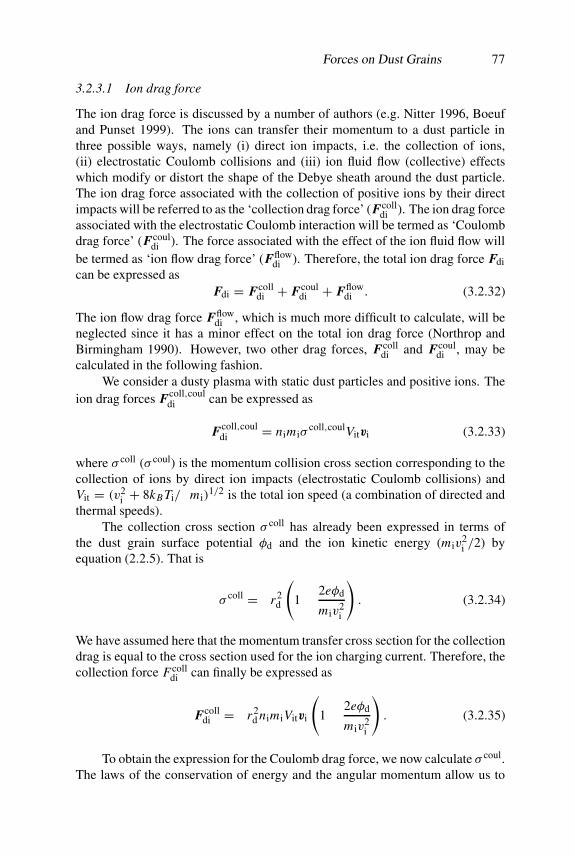
Forces on Dust Grains 77
3.2.3.1 Ion drag force
The ion drag force is discussed by a number of authors (e.g. Nitter 1996, Boeufand Punset 1999). The ions can transfer their momentum to a dust particle inthree possible ways, namely (i) direct ion impacts, i.e. the collection of ions,(ii) electrostatic Coulomb collisions and (iii) ion fluid flow (collective) effectswhich modify or distort the shape of the Debye sheath around the dust particle.The ion drag force associated with the collection of positive ions by their directimpacts will be referred to as the ‘collection drag force’ (Fcoll
di ). The ion drag forceassociated with the electrostatic Coulomb interaction will be termed as ‘Coulombdrag force’ (Fcoul
di ). The force associated with the effect of the ion fluid flow willbe termed as ‘ion flow drag force’ (Fflow
di ). Therefore, the total ion drag force Fdican be expressed as
Fdi = Fcolldi + Fcoul
di + Fflowdi . (3.2.32)
The ion flow drag force Fflowdi , which is much more difficult to calculate, will be
neglected since it has a minor effect on the total ion drag force (Northrop andBirmingham 1990). However, two other drag forces, Fcoll
di and Fcouldi , may be
calculated in the following fashion.We consider a dusty plasma with static dust particles and positive ions. The
ion drag forces Fcoll,couldi can be expressed as
Fcoll,couldi = nimiσ
coll,coulVitvi (3.2.33)
where σ coll (σ coul) is the momentum collision cross section corresponding to thecollection of ions by direct ion impacts (electrostatic Coulomb collisions) andVit = (v2
i + 8kB Ti/πmi)1/2 is the total ion speed (a combination of directed and
thermal speeds).The collection cross section σ coll has already been expressed in terms of
the dust grain surface potential φd and the ion kinetic energy (miv2i /2) by
equation (2.2.5). That is
σ coll = πr2d
(1− 2eφd
miv2i
). (3.2.34)
We have assumed here that the momentum transfer cross section for the collectiondrag is equal to the cross section used for the ion charging current. Therefore, thecollection force Fcoll
di can finally be expressed as
Fcolldi = πr2
d nimiVitvi
(1− 2eφd
miv2i
). (3.2.35)
To obtain the expression for the Coulomb drag force, we now calculate σ coul.The laws of the conservation of energy and the angular momentum allow us to

78 Dynamics of Dust Grains
express the momentum transfer cross section for the Coulomb drag (σ coul) as(Bittencourt 1986, Nitter 1996)
σ coul = 4πb20
∫ λDe
bc
b db
b20 + b2
(3.2.36)
where b is the impact parameter,
b0 = rdeφd
miv2i
(3.2.37)
is the impact radius corresponding to a 90◦ deflection and
bc = rd
(1− 2eφd
miv2i
)1/2
(3.2.38)
is the direct collision impact parameter. Note that the direct collision impactparameter bc is used in order to exclude the collected ions from the calculationof the Coulomb drag force Fcoul
di . If we choose the upper integration limit ofthe integral in equation (3.2.36) at infinity, it diverges. Therefore, it is commonto introduce a cut-off for this upper integration limit at λDe (Nitter 1996). Theelectron Debye length λDe is the appropriate cut-off (or shielding length) in thiscase, because the ions, having a drift speed that is large compared with the ionthermal speed, are unable to form the sheath around the dust particle. Thus,the Debye sheath consists only of a deficiency of electrons, with thickness givenapproximately by λDe. The integration of equation (3.2.36) yields
σ coul = 2πb20 ln
(b2
0 + λ2De
b20 + b2
c
). (3.2.39)
The Coulomb ion drag forces Fcouldi is thus given by
Fcouldi = 2πb2
0nimiVitvi ln
(b2
0 + λ2De
b20 + b2
c
). (3.2.40)
3.2.3.2 Neutral drag force
The neutral drag force may be defined as the rate of momentum exchange betweendust particles and neutrals during their collisions. To estimate the neutral dragforce, there are two regimes to be considered. These are the hydrodynamicregime, where the Knudsen number is much smaller than unity, i.e. Kn (= neutralmean free path/dust particle radius) � 1, and a kinetic regime in which theKnudsen number is much larger than unity, i.e. Kn � 1. In the hydrodynamic(high-pressure) regime, the drag force can be estimated from Stokes’ law and is
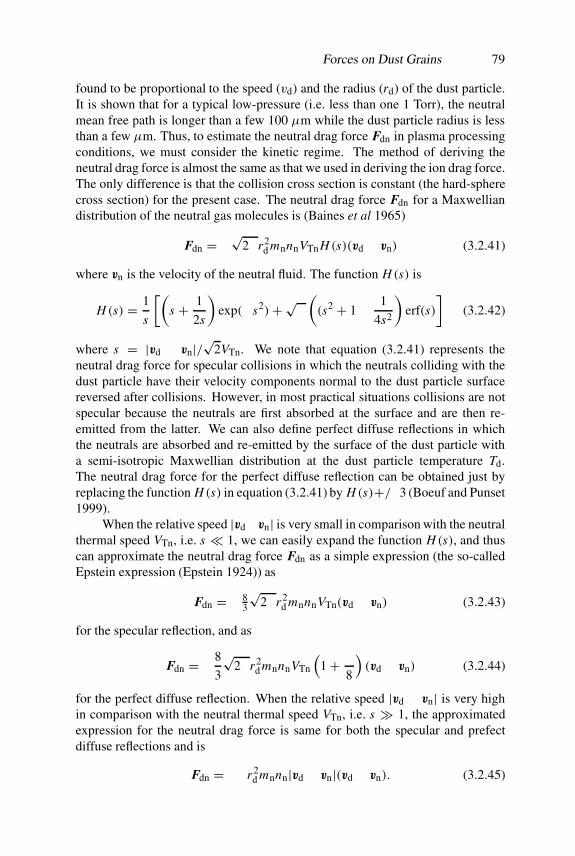
Forces on Dust Grains 79
found to be proportional to the speed (vd) and the radius (rd) of the dust particle.It is shown that for a typical low-pressure (i.e. less than one 1 Torr), the neutralmean free path is longer than a few 100 µm while the dust particle radius is lessthan a few µm. Thus, to estimate the neutral drag force Fdn in plasma processingconditions, we must consider the kinetic regime. The method of deriving theneutral drag force is almost the same as that we used in deriving the ion drag force.The only difference is that the collision cross section is constant (the hard-spherecross section) for the present case. The neutral drag force Fdn for a Maxwelliandistribution of the neutral gas molecules is (Baines et al 1965)
Fdn = −√
2πr2d mnnnVTnH (s)(vd − vn) (3.2.41)
where vn is the velocity of the neutral fluid. The function H (s) is
H (s) = 1
s
[(s + 1
2s
)exp(−s2)+√π
((s2 + 1− 1
4s2
)erf(s)
](3.2.42)
where s = |vd − vn|/√
2VTn. We note that equation (3.2.41) represents theneutral drag force for specular collisions in which the neutrals colliding with thedust particle have their velocity components normal to the dust particle surfacereversed after collisions. However, in most practical situations collisions are notspecular because the neutrals are first absorbed at the surface and are then re-emitted from the latter. We can also define perfect diffuse reflections in whichthe neutrals are absorbed and re-emitted by the surface of the dust particle witha semi-isotropic Maxwellian distribution at the dust particle temperature Td.The neutral drag force for the perfect diffuse reflection can be obtained just byreplacing the function H (s) in equation (3.2.41) by H (s)+π/3 (Boeuf and Punset1999).
When the relative speed |vd−vn| is very small in comparison with the neutralthermal speed VTn, i.e. s � 1, we can easily expand the function H (s), and thuscan approximate the neutral drag force Fdn as a simple expression (the so-calledEpstein expression (Epstein 1924)) as
Fdn = − 83
√2πr2
d mnnnVTn(vd − vn) (3.2.43)
for the specular reflection, and as
Fdn = −8
3
√2πr2
d mnnnVTn
(1+ π
8
)(vd − vn) (3.2.44)
for the perfect diffuse reflection. When the relative speed |vd − vn| is very highin comparison with the neutral thermal speed VTn, i.e. s � 1, the approximatedexpression for the neutral drag force is same for both the specular and prefectdiffuse reflections and is
Fdn = −πr2d mnnn|vd − vn|(vd − vn). (3.2.45)

80 Dynamics of Dust Grains
It is important to point out that in a realistic laboratory dusty plasma situationwe have s � 1, and the Epstein limit is a good approximation for calculatingthe neutral drag force. Draine and Salpeter (1979) have considered the specularreflection and derived an approximate expression for the neutral drag force
Fdn = −8
3
√2πr2
d mnnnVTn
(1+ 9π
64s2)1/2
(vd − vn) (3.2.46)
which is accurate to within 1% for all velocities and exact in the limits s → 0 ands →∞. The specular and perfect diffuse reflections that we have considered arejust two extreme assumptions for collisions between dust particles and neutrals.To account for the intermediate situation, one can use the accommodationcoefficient αac, which measures the probability of a perfect diffuse reflectionand depends on the surface properties of the dust particle. Knudsen (1991)first introduced the accommodation coefficient to take into account the fact thatabsorbed neutrals do not necessarily reach thermal equilibrium with the particlesurface before they are absorbed. Using the accommodation coefficient αac, theneutral drag force Fdn in the Epstein limit (s � 1) becomes (Perrin et al 1994,Boeuf and Punset 1999)
Fdn = −8
3
√2πr2
d mnnnVTn
(1+ αac
π
8
)(vd − vn). (3.2.47)
Note that the accommodation coefficient αac would be zero for specular reflectionand unity for perfect diffuse reflection.
3.2.4 Thermophoretic force
We consider a dust particle that resides in a neutral gas with a temperature gradient∇Tn. The molecules on the hot side of the particle have higher thermal speedsthan those on the cold side. This means that a net momentum transfer fromthe gas to the dust particle occurs (since the momentum transfer rate from thegas to the dust particle depends upon the speed of the molecules). The rateof this net momentum transfer is known as the thermophoretic force FT. Itsmagnitude is directly proportional to the temperature gradient and its directionis in the direction of the heat flux, i.e. in the direction opposite to the neutral gastemperature gradient.
Talbot et al (1980), who assumed that the non-uniform velocity distributionof the unperturbed neutral gas in the vicinity of the dust particle can berepresented in the Chapman–Enskog form and that the particle is small enoughto influence this distribution function, have analytically derived the expressionfor the thermophoretic force. Daugherty and Graves (1995) have also physicallyexplained this force in order to understand a particulate transport model for aglow discharge. The thermophoretic force FT acting on a dust particle for a non-uniform (unperturbed) gas velocity distribution of the Chapman–Enskog form is

Forces on Dust Grains 81
given by (Talbot et al 1980, Daugherty and Graves 1995)
FT = −8√
2π
15
r2d
VTn
[1+ 5π
32(1− αac)
]kcon
n ∇Tn (3.2.48)
where kconn is the translational thermal conductivity of the neutral gas. Talbot et
al (1980) have suggested that for gas and dust having temperatures less than 500K, the accommodation coefficient αac can be close to unity. As in most spaceand laboratory dusty plasmas the neutral temperature is below/around the roomtemperature, we can set αac = 1. On the other hand, using the Chapman–Enskogexpression for the thermal conductivity we can express kcon
n as (Daugherty andGraves 1995)
kconn = 75
64√π
kB VTn
σ 2LJ�
!LJ
(3.2.49)
where σLJ is the Lennard-Jones collision diameter of the gas and �!LJ is a collision
integral for scattering in a Lennard-Jones potential. The asterisk indicates thatthe collision integral has been reduced by its value for hard-sphere scattering.The integral �!
LJ is a weak function of the temperature, and its value is closeto unity for most mono-polar gases near room temperature (Daugherty andGraves 1995). Therefore, substituting equation (3.2.49) into equation (3.2.48)the thermophoretic force FT can be simplified as
FT � − 5
4√
2
(rd
σLJ
)2
kB∇Tn. (3.2.50)
Now if we can consider ∇Tn in equation (3.2.50) to be an independent variable,the thermophoretic force FT is independent of the neutral pressure and the massof the neutral gas. However, this is only true if the neutral pressure is so high thatthe number of the neutral mean free path between the dust particle and the systemboundaries is much larger than one (Daugherty and Graves 1995). Of course, ifthe pressure approaches zero, the thermophoretic force must eventually approachzero because at sufficiently low pressure collisions between the neutrals and thedust particles cease. However, if the mean free path is of the order of the systemsize, a thermophoretic force can still exist, although the velocity distribution willno longer take the Chapman–Enskog form. This effect has been considered byHavnes et al (1994) who found that the thermophoretic force is reduced by afactor ∼2 within one mean free path of the wall.
We have discussed the thermophoretic force associated with the neutraltemperature gradient. It is conceivable that temperature gradients in the ion andelectron fluids could result in an additional contribution to the thermophoreticforce. This possibility has been addressed by several authors (e.g. Chen andTao 1992, Daugherty and Graves 1995). It is reasonable that the thermophoreticforce from neutrals in equation (3.2.46) scales as hard-sphere cross section∼r2
d , and we might expect the thermophoretic force to scale as the screened

82 Dynamics of Dust Grains
Coulomb cross section∼λ2D. At first glance it might seem that the thermophoretic
force associated with the ion and electron temperature gradients dominatesthat associated with neutral temperature gradient because rd � λD, and thethermophoretic force is apparently independent of the gas density and the mass ofthe colliding species. However, in a weakly ionized gas ion–neutral and electron–neutral collisions are usually much more important than ion-ion or electron–electron self-collisions, and this leads to a different functional form of the thermalconductivity for these species. The thermal conductivity kcon
e,i of the electrons andions has the general functionality given by (Daugherty and Graves 1995)
kcone,i �
ne,ikB V 2Te,i
νe,i(3.2.51)
where the subscript e (i) represents the corresponding quantity for the electron(ion) and νe (νi) is the collision frequency of the electrons (ions). As the dominantpart of νe (νi) is usually due to collisions of electrons (ions) with the neutrals,from equation (1.2.14) we have νe,i � νen,in = nnσ
ne,iVTe,i. This reduces the ion
or electron thermal conductivity kcone,i to the form
kcone,i �
ne,i
nn
kB VTe,i
σ ne,i
. (3.2.52)
Since in partially ionized dusty plasmas ne,i/nn is seldom larger than 10−6 andVTe,i cancels out when equation (3.2.52) is substituted into the thermophoreticforce, it appears that the ion and electron thermophoretic forces will not beparticularly important unless the temperature gradients are very large. However,in a high-density plasma (e.g. electron cyclotron resonances (ECR), inductivelycoupled plasma (ICP), helicon plasma, etc) the ratio ne,i/nn may be as large as0.1, and in this case one must consider ion and electron thermophoretic forcesmore seriously.
3.2.5 Radiation pressure force
We know that dust particles (particularly in space) are immersed in anenvironment of electromagnetic waves/radiation emitted from various sources andare therefore continuously irradiated. Thus, an irradiated dust particle interceptsa fraction of the radiation energy ER and associated momentum PR = ER/c.To estimate the force, i.e. the rate of the momentum transfer to a dust particle,we consider the electromagnetic radiation as a beam of photons, each of whichhas energy E (1)
R = hωR and momentum P(1)R = E (1)
R /c, where ωR is theradiation angular frequency. The intensity of the electromagnetic radiation is thencharacterized by the photon energy flux (photon energy distributed per unit areaper unit time) I0 = NphhωRc, where Nph is the photon number density. Thus, the
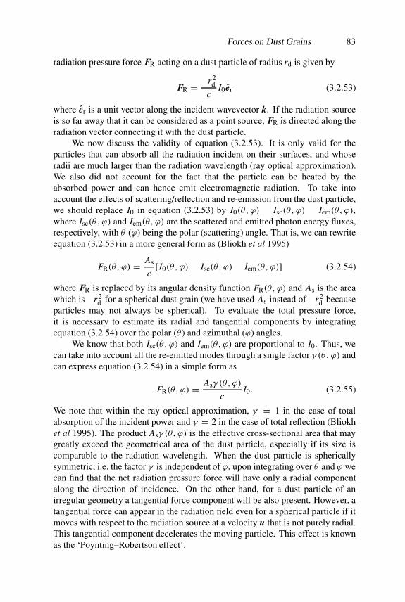
Forces on Dust Grains 83
radiation pressure force FR acting on a dust particle of radius rd is given by
FR = πr2d
cI0 er (3.2.53)
where er is a unit vector along the incident wavevector k. If the radiation sourceis so far away that it can be considered as a point source, FR is directed along theradiation vector connecting it with the dust particle.
We now discuss the validity of equation (3.2.53). It is only valid for theparticles that can absorb all the radiation incident on their surfaces, and whoseradii are much larger than the radiation wavelength (ray optical approximation).We also did not account for the fact that the particle can be heated by theabsorbed power and can hence emit electromagnetic radiation. To take intoaccount the effects of scattering/reflection and re-emission from the dust particle,we should replace I0 in equation (3.2.53) by I0(θ, ϕ) − Isc(θ, ϕ) − Iem(θ, ϕ),where Isc(θ, ϕ) and Iem(θ, ϕ) are the scattered and emitted photon energy fluxes,respectively, with θ (ϕ) being the polar (scattering) angle. That is, we can rewriteequation (3.2.53) in a more general form as (Bliokh et al 1995)
FR(θ, ϕ) = As
c[I0(θ, ϕ)− Isc(θ, ϕ)− Iem(θ, ϕ)] (3.2.54)
where FR is replaced by its angular density function FR(θ, ϕ) and As is the areawhich is πr2
d for a spherical dust grain (we have used As instead of πr2d because
particles may not always be spherical). To evaluate the total pressure force,it is necessary to estimate its radial and tangential components by integratingequation (3.2.54) over the polar (θ ) and azimuthal (ϕ) angles.
We know that both Isc(θ, ϕ) and Iem(θ, ϕ) are proportional to I0. Thus, wecan take into account all the re-emitted modes through a single factor γ (θ, ϕ) andcan express equation (3.2.54) in a simple form as
FR(θ, ϕ) = Asγ (θ, ϕ)
cI0. (3.2.55)
We note that within the ray optical approximation, γ = 1 in the case of totalabsorption of the incident power and γ = 2 in the case of total reflection (Bliokhet al 1995). The product Asγ (θ, ϕ) is the effective cross-sectional area that maygreatly exceed the geometrical area of the dust particle, especially if its size iscomparable to the radiation wavelength. When the dust particle is sphericallysymmetric, i.e. the factor γ is independent of ϕ, upon integrating over θ and ϕ wecan find that the net radiation pressure force will have only a radial componentalong the direction of incidence. On the other hand, for a dust particle of anirregular geometry a tangential force component will be also present. However, atangential force can appear in the radiation field even for a spherical particle if itmoves with respect to the radiation source at a velocity u that is not purely radial.This tangential component decelerates the moving particle. This effect is knownas the ‘Poynting–Robertson effect’.

84 Dynamics of Dust Grains
We can explain this effect clearly by considering scattering and emissionof the radiation in a frame of reference moving with the particle, i.e. movingwith the dust velocity vd. To make equation (3.2.53), which we have derivedfor a particle at rest, valid for this moving frame, we should take into accountthe Doppler and aberration effects. Because of the Doppler effect the frequencyof the radiation incident of the particle will be ωR(1 − ur/c), where ur is theradial component of u and the photon momentum P(1)
R = hωR(1 − ur/c) will bechanged in magnitude. On the other hand, owing to the aberration the wave willpropagate at an angle �θ = uθ /c, where uθ is the tangential component of u. Asa result, the axial symmetry with respect to the radial direction will be violatedand a tangential force component will develop. These two considerations allowus to rewrite equation (3.2.54) as (Bliokh et al 1995)
FR = Asγ
cI0
[(1− ur
c
)er − uθ
ceθ]
(3.2.56)
where eθ is the tangential unit vector, eθ ⊥ er. Due to the tangential component ofthe radiation pressure force, a particle orbiting around the attraction centre, whichat the same time is the radiation source (e.g. the Sun), is continuously sloweddown. Because of this decelerating force, known as the ‘radiation drag force’, theparticle loses a part of its energy and its orbital radius decreases. Consequently,the particle moves closer to the radiation source.
Now an important question may arise: will the radiation pressure force besignificantly changed if an electric charge qd possibly carried by the dust grainis taken into consideration? Let us present an answer to this question. The forceacting on a charged dust particle in an electric field is qd E0 exp(−iωRt + ik · r),where E0 is the amplitude of the electric field vector. It produces periodicoscillations of the dust grain which thus becomes a source of electromagneticradiation of the same frequency ωR. The power radiated by the vibratingparticle comes from the primary electromagnetic wave. The dust particle thusreceives some power along with a fraction of the wave momentum by whichequation (3.2.53) is affected. This effect can be included by using an effectivecross-sectional area σef instead of the geometric cross-sectional area πr2
d . Theeffective cross-sectional area σef corresponds to that fraction of the wave powerwhich is transformed into the radiation scattered by the charge qd and can beestimated by using the Thomson scattering formula as
σef = 8π
3
(q2
d
mdc2
)2
. (3.2.57)
It is seen that the effective (charge dependent) cross section σef involves thegrain radius only implicitly through qd � rdφd and md = (4π/3)r3
dρd, whereρd is the mass density of the dust material, and can be written as σef �(9/16π2)φ4
d/r2dρ
2d c4. This implies that the effective cross section σef is inversely
proportional to r2d , whereas the geometric cross section is directly proportional to
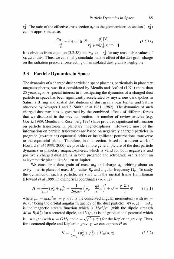
Particle Dynamics in Space 85
r2d . The ratio of the effective cross section σef to the geometric cross section (πr2
d )can be approximated as
σef
πr2d
� 4.4× 10−39 φ4d[V]
r4d [µm]ρ2
d [g cm−3] . (3.2.58)
It is obvious from equation (3.2.58) that σef � πr2d for any reasonable values of
rd, ρd and φd. Thus, we can finally conclude that the effect of the dust grain chargeon the radiation pressure force acting on an isolated dust grain is negligible.
3.3 Particle Dynamics in Space
The dynamics of a charged dust particle in space plasmas, particularly in planetarymagnetospheres, was first considered by Mendis and Axford (1974) more than25 years ago. A special interest in investigating the dynamics of a charged dustparticle in space has been significantly accelerated by mysterious dark spokes inSaturn’s B ring and spatial distributions of dust grains near Jupiter and Saturnobserved by Voyager 1 and 2 (Smith et al 1981, 1982). The dynamics of suchcharged dust particles is governed by the combined effects of different forcesthat we discussed in the previous section. A number of review articles (e.g.Goertz 1989, Mendis and Rosenberg 1994) have provided significant informationon particle trajectories in planetary magnetospheres. However, most of theinformation on particle trajectories are based on negatively charged particles inprograde (co-rotating) equatorial orbits or insignificant perturbations transverseto the equatorial plane. Therefore, in this section, based on a recent work ofHoward et al (1999, 2000) we provide a more general picture of the dust particledynamics in planetary magnetospheres, which is valid for both negatively andpositively charged dust grains in both prograde and retrograde orbits about anaxisymmetric planet like Saturn or Jupiter.
We consider a dust grain of mass md and charge qd orbiting about anaxisymmetric planet of mass Mp, radius Rp and angular frequency �pl. To studythe dynamics of such a particle, we start with the inertial frame Hamiltonian(Howard et al 1999) in cylindrical coordinates (ρ, ϕ, z)
H = 1
2md(p2
ρ + p2z )+
1
2mdρ2
(pϕ − qd
c#)2 +U + qd�pl
c# (3.3.1)
where pϕ = mdρ2ωd + qd#/c is the conserved angular momentum (with ωd =
∂ϕ/∂ t being the orbital angular frequency of the dust particle), #(ρ, z) = ρAϕ
is the magnetic stream function which is Mρ2/r3 (with the dipole strengthM = B0 R3
p) for a centered dipole, and U(ρ, z) is the gravitational potential which
is −µmd/r (with µ = GMp and r = √ρ2 + z2) for the Keplerian gravity. Thus,for a centered dipole and Keplerian gravity, we can express H as
H = 1
2md(p2
ρ + p2z )+Uef(ρ, z) (3.3.2)
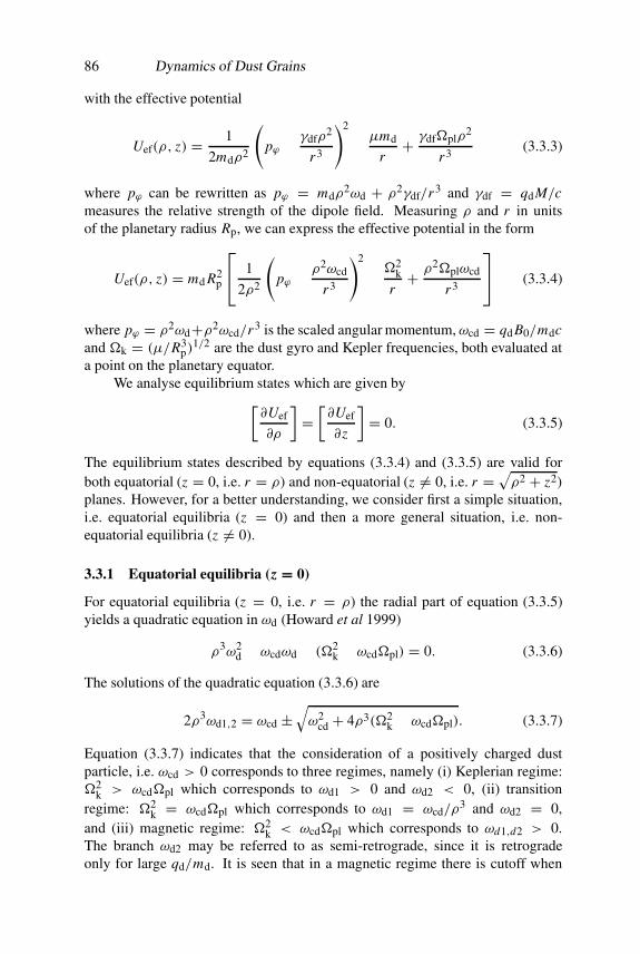
86 Dynamics of Dust Grains
with the effective potential
Uef(ρ, z) = 1
2mdρ2
(pϕ − γdfρ
2
r3
)2
− µmd
r+ γdf�plρ
2
r3(3.3.3)
where pϕ can be rewritten as pϕ = mdρ2ωd + ρ2γdf/r3 and γdf = qdM/c
measures the relative strength of the dipole field. Measuring ρ and r in unitsof the planetary radius Rp, we can express the effective potential in the form
Uef(ρ, z) = md R2p
1
2ρ2
(pϕ − ρ2ωcd
r3
)2
− �2k
r+ ρ2�plωcd
r3
(3.3.4)
where pϕ = ρ2ωd+ρ2ωcd/r3 is the scaled angular momentum,ωcd = qd B0/mdcand �k = (µ/R3
p)1/2 are the dust gyro and Kepler frequencies, both evaluated at
a point on the planetary equator.We analyse equilibrium states which are given by[
∂Uef
∂ρ
]=[∂Uef
∂z
]= 0. (3.3.5)
The equilibrium states described by equations (3.3.4) and (3.3.5) are valid forboth equatorial (z = 0, i.e. r = ρ) and non-equatorial (z �= 0, i.e. r = √ρ2 + z2)planes. However, for a better understanding, we consider first a simple situation,i.e. equatorial equilibria (z = 0) and then a more general situation, i.e. non-equatorial equilibria (z �= 0).
3.3.1 Equatorial equilibria (z = 0)
For equatorial equilibria (z = 0, i.e. r = ρ) the radial part of equation (3.3.5)yields a quadratic equation in ωd (Howard et al 1999)
ρ3ω2d − ωcdωd − (�2
k − ωcd�pl) = 0. (3.3.6)
The solutions of the quadratic equation (3.3.6) are
2ρ3ωd1,2 = ωcd ±√ω2
cd + 4ρ3(�2k − ωcd�pl). (3.3.7)
Equation (3.3.7) indicates that the consideration of a positively charged dustparticle, i.e. ωcd > 0 corresponds to three regimes, namely (i) Keplerian regime:�2
k > ωcd�pl which corresponds to ωd1 > 0 and ωd2 < 0, (ii) transitionregime: �2
k = ωcd�pl which corresponds to ωd1 = ωcd/ρ3 and ωd2 = 0,
and (iii) magnetic regime: �2k < ωcd�pl which corresponds to ωd1,d2 > 0.
The branch ωd2 may be referred to as semi-retrograde, since it is retrogradeonly for large qd/md. It is seen that in a magnetic regime there is cutoff when

Particle Dynamics in Space 87
ω2cd = 4ρ3(ωcd�pl−�2
k) which is itself a quadratic in ωcd. It can be easily shownthat this inner quadratic has real roots only for ρ > (�k/�pl)
2/3. Equation (3.3.7)also implies that for a negatively charged dust particle (ωcd < 0), we can consideronly one situation, namely ωd1 > 0, ωd2 < 0. Obviously there is no cutoff:a pair of prograde–retrograde orbits exist everywhere on the equatorial plane.Figure 3.1 shows the orbital frequencies (normalized by the Kepler frequency)ωd1,2/�k as a function of ωcd/�k for (a) ρ = 1.5 and (b) ρ = 2.0 for bothpositively and negatively changed dust particles. The asymptotes are shown asdashed lines. We note that as ρ = 1.882 = ρs corresponds to the synchronousradius in the case of Saturn, figure 3.1(a) represents orbital frequencies insidethe synchronous radius (ρ < ρs) and figure 3.1(b) represents orbital frequenciesoutside the synchronous radius (ρ > ρs). It may also be noted here that whenωcd → 0, ωd1,2 → ±�k/ρ
3/2 (the local Kepler frequency) and when ρ < ρsand qd/md lies within the limit of large positive values, ωd1 → ωcd/ρ
3 (the localgyrofrequency), ωd2 → �pl. On the other hand, when ρ < ρs and qd/md lieswithin the limit of large negative values, ωd1 → �pl, ωd2 →−ωcd/ρ
3.
3.3.2 Non-equatorial equilibria (z �= 0)
The simultaneous solutions of equation (3.3.5) for z �= 0 are given by (Howard etal 2000)
r5ω2d + ωcd(ωd −�pl)(2r2 − 3ρ2) = �2
kr2 (3.3.8)
and3ωcd(ωd −�pl)ρ
2 +�2kr2 = 0. (3.3.9)
It follows immediately from equation (3.3.9) that the orbital frequency ωd �=�pl, i.e. non-equatorial synchronous orbits are not possible. We also see fromequation (3.3.9) that for a positively charged dust grain ωd < �pl, whereas for anegatively charged grain ωd > �pl. The latter also holds for equatorial orbits.
We know that for a spherical dust grain of a uniform material densityρd � 1 g cm−3, radius rd (in microns) and a surface potential φd (in volts)qd/md � (106/4π)φd/r2
d esu g−1. Typical values of φd for Jupiter and Saturnlie in the range −20 V < φd < 10 V (Howard et al 1999, 2000). For a givenplanet and an equilibrium radial position r0, the stability of the dust particle orbitdepends on qd/md alone, conveniently measured by the parameter $ = φd/r2
d =(4πc/106B0)ωcd, which we shall express as a pure number. We now analysewhether a stable equilibrium orbit exists for some $, i.e. for some ωcd for aspecific location (ρ0, z0). We first eliminate ωcd between equations (3.3.8) and(3.3.9) and obtain
ω2d =
2
3
�2k
ρ20r0
. (3.3.10)
It is seen that both signs of ωd are possible. The requisite value of $(ωcd) (if it

88 Dynamics of Dust Grains
Figure 3.1. The orbital frequencies (normalized by the Kepler frequency) ωd1,2/�k as afunction of ωcd/�k for (a) ρ = 1.5 and (b) ρ = 2.0 (after Howard et al 1999).

Particle Dynamics in Laboratory 89
exists) is then determined from
ωcd = ω2dr3
0
2(�pl − ωd). (3.3.11)
It is obvious that when dust particles are positively charged, equation (3.3.11) isautomatically satisfied for negative (retrograde) ωd but demands ωd < �pl forpositive (prograde) ωd. On the other hand, when dust particles are negativelycharged, this will be only satisfied if ωd > �pl > 0, which excludes retrogradeorbits. There are no retrograde non-equatorial equilibria for negative charge, buteither sense is possible for positive charge (Howard et al 2000). We now take thepoint of view that r0 and ωcd are specified and seek conditions for an equilibriumsomewhere on the sphere r = r0. We can express equation (3.3.11) as a quadraticin ωd and find its solution as
r30ωd = −ωcd ±
√ω2
cd + 2r30�plωcd (3.3.12)
which is subjected to the constraint ρ < r . Thus, equation (3.3.10) impliesω2
d ≥ ω2! = 2�2
k/3r20 , with corresponding ωcd given by equation (3.3.11), which
yields (ω! > 0)�2
k
3(�pl + ω!)≤ ωcd ≤ �2
k
3(�pl − ω!). (3.3.13)
The numerical solutions of equation (3.3.12) for r0 = 2 are shown in figure 3.2.This shows that for ωcd > 0 and |ωd| > ω! there is a prograde/retrogradepair, but for −2r3
0� < ωcd < 0 there are no equilibria. It also shows that ifωcd < −2r3
0�pl, there are two possible prograde equilibria. Since ω! < �pl thereare no constraints in qd/md. However, for large qd/md there are two asymptoticlimits: ωd � �pl and ωd � −�pl − 2ωcd/r3
0 .
3.4 Particle Dynamics in Laboratory
The dynamics of a dust particle in a laboratory plasma, particularly in the plasmasheath boundary of a gas discharge under a time varying background gas pressure,is an extremely complex problem due to both the nature of the plasma sheathand the charging currents that reach the dust grain surface. However, a numberof approximations and simplifications may make possible a treatment of such acomplicated problem. Recently, Winske and Jones (1994), Elskens et al (1997)and Resendes and Shukla (2001) have investigated the dynamics of a dust particlein the plasma sheath boundary by using a fluid (so-called continuum) model whichprimarily involves calculating the electron and ion densities, the electric fieldand the dust grain charge under different approximations and simplifications. Toprovide some basic understanding of the dust particle dynamics in the plasmasheath, here we will briefly summarize the work of Resendes and Shukla (2001).
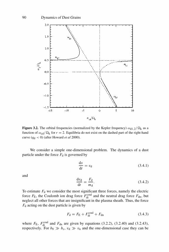
90 Dynamics of Dust Grains
Figure 3.2. The orbital frequencies (normalized by the Kepler frequency) ωd1,2/�k as afunction of ωcd/�k for r = 2. Equilibria do not exist on the dashed part of the right-handcurve (qd < 0) (after Howard et al 2000).
We consider a simple one-dimensional problem. The dynamics of a dustparticle under the force Fd is governed by
dx
dt= vd (3.4.1)
anddvd
dt= Fd
md. (3.4.2)
To estimate Fd we consider the most significant three forces, namely the electricforce FE, the Coulomb ion drag force Fcoul
di and the neutral drag force Fdn, butneglect all other forces that are insignificant in the plasma sheath. Thus, the forceFd acting on the dust particle is given by
Fd = FE + Fcouldi + Fdn (3.4.3)
where FE, Fcouldi and Fdn are given by equations (3.2.2), (3.2.40) and (3.2.43),
respectively. For b0 � bc, vd � vn and the one-dimensional case they can be
Particle Dynamics in Laboratory 91
expressed as
FE = qd E (3.4.4)
Fcouldi = 2πnimiVitvib
20 ln
(1+ λ2
De
b20
)(3.4.5)
andFdn = − 8
3
√2πr2
d mnnnVTnvd (3.4.6)
where b0 is given by equation (3.2.37) and can be expressed in terms of the dustparticle charge as b0 = eqd/mv2
i . The charge qd of a dust particle in a laboratoryplasma environment (particularly in the plasma sheath boundary) is not constantbut varies with space. To estimate qd we consider only the orbit-limited chargingcurrents that are due to the collection of primary plasma particles (electrons andions). As the ions are much heavier than the electrons, initially the ion current ismuch smaller than the electron current, and the grain becomes negatively charged(i.e. qd < 0). This increases the ion current Ii and decreases the electron currentIe until Ie + Ii = 0, where Ie and Ii are given by equations (2.6.2) and (2.6.11).Thus, the dust grain charge qd (< 0) can be determined from Ie+ Ii = 0, yielding
ne
ni
(Temi
Time
)1/2
exp
(eqd
rdkB Te
)=(
1+ π
8
v2i
V 2T i
)1/2(1− 2eqd
rdmiV 2it
)(3.4.7)
where we have taken the ion speed as its total speed Vit (a combination of directedand thermal speeds). It is clear from equations (3.4.1)–(3.4.7) that in order tosolve equations (3.4.1) and (3.4.2) we still need to know four other variables,namely ne, ni, vi and E .
To estimate these variables we consider a simple one-dimensional, time-independent glow discharge model (Winske and Jones 1994, Resendes and Shukla2001) which employs the usual diffusion approximation to solve numericallythe electron and ion continuity equations, the electron momentum equation andPoisson’s equation, which are, respectively,
dJe
dx= neνi (3.4.8)
dJi
dx= neνi (3.4.9)
dne
dx= − 1
De(Je + neµe E) (3.4.10)
anddE
dx= 4πe(ni − ne) (3.4.11)
where Je = neve and Ji � niµi E are electron and ion fluxes, respectively, νi =nn Ki exp(−Ei/kB Te), µe (= 6×107 cm2/statV s) and µi (= 6×105 cm2/statV s)
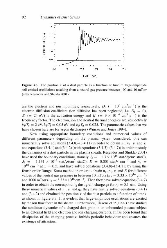
92 Dynamics of Dust Grains
Figure 3.3. The position x of a dust particle as a function of time t : large-amplitudeself-excited oscillations resulting from a neutral gas pressure between 100 and 10 mTorr(after Resendes and Shukla 2001).
are the electron and ion mobilities, respectively, De (= 106 cm2/s−1) is theelectron diffusion coefficient (ion diffusion has been neglected, i.e. Di = 0),Ei (= 24 eV) is the activation energy and Ki (= 9 × 10⁻⁶ cm3 s−1) is thefrequency factor. The electron, ion and neutral thermal energies are, respectivelykB Te = 2 eV, kB Ti = 0.05 eV and kB Tn = 0.025. The parametric values that wehave chosen here are for argon discharges (Winske and Jones 1994).
Now using appropriate boundary conditions and numerical values ofdifferent parameters depending on the plasma system considered, one cannumerically solve equations (3.4.8)–(3.4.11) in order to obtain ni, ne, vi and Eand equations (3.4.1) and (3.4.2) (with equations (3.4.3)–(3.4.7)) in order to studythe dynamics of a dust particle in the plasma sheath. Resendes and Shukla (2001)have used the boundary conditions, namely Je = −1.3× 10¹⁵ statA/(cm2 statC),Ji = −1.131 × 10¹⁶ statA/(cm2 statC), E = 0.001 statV cm−1 and ne =1010 cm−3 at x = 0.5, and have solved equations (3.4.8)–(3.4.11) by using thefourth order Runge–Kutta method in order to obtain ne, ni, vi and E for differentvalues of the neutral gas pressure in between 10 mTorr (nn = 3.33× 1014 cm−3)and 1000 mTorr (nn = 3.33×1016 cm−3). Then they have solved equation (3.4.7)in order to obtain the corresponding dust grain charge qd for rd = 0.1 µm. Usingthese numerical values of ni, vi and qd they have finally solved equations (3.4.1)and (3.4.2) and obtained the position x of the dust particle as a function of time tas shown in figure 3.3. It is evident that large-amplitude oscillations are excitedby the ion flow force in the sheath. Furthermore, Elskens et al (1997) have studiedthe nonlinear dynamics of a charged dust grain in an unbounded plasma subjectto an external field and electron and ion charging currents. It has been found thatdissipation of the charging process forbids periodic behaviour and ensures theexistence of attractors.

Chapter 4
Linear Waves
4.1 Introduction
The charged particles in a plasma move randomly, interact with each otherthrough their own electromagnetic forces, and also respond to perturbations thatare applied externally. Therefore, a great variety of collective wave phenomenaarises due to the coherent motions of an ensemble of plasma particles. Itis well known (Ichimaru 1973, Chen 1974, Alexandrov et al 1984) that anelectron–ion plasma supports both longitudinal and transverse waves. Examplesof longitudinal waves in an unmagnetized plasma are Langmuir and ion-acoustic waves which are accompanied with density and potential fluctuations.On the other hand, transverse waves in an unmagnetized plasma are purelyelectromagnetic and they do not accompany density fluctuations. The presence ofan external magnetic field in a plasma provides the possibility of a great varietyof longitudinal and transverse waves.
When neutral dust grains are added in an electron–ion plasma, they arecharged due to a variety of processes, as described in chapter 2. The presenceof charged dust grains can modify or even dominate the wave propagation (Rao etal 1990, Shukla and Silin 1992, Verheest 2000, Shukla 2001). The modificationof the wave phenomena occurs owing to the inhomogeneity associated withthe random distribution of the charged particulates and the departure from theconventional quasi-neutrality condition in an electron–ion plasma due to thepresence of charged dust grains, as well as due to the consideration of the dustparticle dynamics. The quasi-neutrality condition at the equilibrium in a dustyplasma with singly charged ions is (cf equation (1.1.1))
eni0 − ene0 + qd0nd0 = 0. (4.1.1)
Using
qd0nd0 = rdφdnd0 ≡ 4πnd0rdλ2Dene0e
eφd
kBTe(4.1.2)
93
94 Linear Waves
we obtain from equation (4.1.1)
ni0
ne0≡ δ = 1− Pde
eφd
kBTe(4.1.3)
where Pde = 4πnd0rdλ2De is a dust parameter. Equation (4.1.3) shows that δ
is larger (smaller) than one for negatively (positively) charged dust grains forwhich φd < 0 (φd > 0). In most of the laboratory dusty plasmas, we havePdee|φd|/kBTe ≤ 1. However, when most of the electrons from the backgroundplasma stick onto the dust grain surface, we have from equation (4.1.1)
ni0 ≈ Pdini0e|φd|kBTi
(4.1.4)
for ne0 � ni0, where Pdi = 4πnd0rdλ2Di. On the other hand, when the dust grains
are positively charged and most of the ions from the background plasma stickonto the dust grain surface, we have from equation (4.1.3)
ne0 ≈ Pdene0e|φd|kBTe
(4.1.5)
for ni0 � ne0. Equations (4.1.4) and (4.1.5) exhibit new types of quasi-neutralityconditions in negative dust–ion and positive dust–electron plasmas, respectively.
In this chapter, we discuss the properties of low-frequency longitudinal andtransverse waves in dusty plasmas which are either unmagnetized or magnetized.The weakly coupled dusty plasma model used here is valid if the grain radius rd aswell as the average intergrain spacing a are much smaller than the dusty plasmaDebye radius λD and the thermal ion gyroradius ρTi (if the ambient magneticfield is present). We also assume that there is a sufficient number of dust grainswithin the dusty plasma Debye sphere so that grains can participate in collectiveinteractions.
4.2 Acoustic Modes
There are two types of acoustic modes in uniform, unmagnetized, collisionlessdusty plasmas with a weak Coulomb coupling between the charged dust grains.These are the dust acoustic (DA) and dust ion-acoustic (DIA) waves. In thefollowing, we describe the underlying physics as well as the mathematical detailsof these wave modes.
4.2.1 Dust acoustic waves
The DA waves have been theoretically predicted by Rao et al (1990) in a multi-component collisionless dusty plasma whose constituents are the electrons, ionsand negatively charged dust grains. The phase velocity of the DA waves is much

Acoustic Modes 95
smaller than the electron and ion thermal speeds. Accordingly, the inertialesselectrons and ions establish equilibrium in the DA wave potential φ. Here thepressure gradient is balanced by the electric force, leading to Boltzmann electronand ion number density perturbations n j1, which are, respectively,
ne1 ≈ ne0eφ
kBTe(4.2.1)
and
ni1 ≈ −ni0eφ
kBTi. (4.2.2)
The dust inertia is very important for the DA waves. Accordingly, the dust numberdensity perturbation is obtained from the dust continuity equation
∂nd1
∂ t+ nd0∇ · vd = 0 (4.2.3)
and the dust momentum equation
∂vd
∂ t= −qd0
md∇φ − 3kBTd
mdnd0∇nd1 (4.2.4)
where nd1 and vd are the dust number density perturbation and the dust fluidvelocity, respectively. Equations (4.2.1)–(4.2.4) are closed by Poisson’s equation
∇2φ = 4π(ene1 − qd0nd1 − eni1) (4.2.5)
where, for convenience, the dust charge qd0 is assumed to be constant. The effectof dust charge fluctuations will be considered in section 4.3.
Let us now derive the dispersion relation for the DA waves. For this purposewe combine equations (4.2.3) and (4.2.4) and obtain(
∂2
∂ t2 − 3V 2Td∇2
)nd1 = nd0qd0
md∇2φ. (4.2.6)
Substituting equations (4.2.1) and (4.2.2) into equation (4.2.5) we have
∇2φ = k2Dφ − 4πqd0nd1. (4.2.7)
Assuming nd1 = nd1 exp(−iωt + ik · r) and φ = φ exp(−iωt + ik · r), whereω and k are the frequency and the wavevector, respectively, we Fourier transformequations (4.2.6) and (4.2.7) (i.e. set ∂/∂ t = −iω and ∇ = ik) and combine theresultant equations to obtain the dispersion relation for the DA waves
1+ k2D
k2 −ω2
pd
ω2 − 3k2V 2Td
= 0 (4.2.8)
96 Linear Waves
which gives
ω2 = 3k2V 2Td +
k2C2D
1+ k2λ2D
(4.2.9)
where CD = ωpdλD is the DA speed. Since ω � kVTd, we deduce fromequation (4.2.9) the DA wave frequency (Rao et al 1990)
ω = kCD
(1+ k2λ2D)
1/2(4.2.10)
which in the long-wavelength limit (namely k2λ2D � 1) reduces to
ω = k Zd0
(nd0
ni0
)1/2(kBTi
md
)1/2 [1+ Ti
Te
(1− Zd0nd0
ni0
)]−1/2
(4.2.11)
when the dust grains are charged negatively. Equation (4.2.11) reveals that therestoring force in the DA waves comes from the pressures of the inertialesselectrons and ions, while the dust mass provides the inertia to support the waves.The frequency of the DA waves is much smaller than the dust plasma frequency.Using equation (4.2.11), the DA wave phase velocity (Vp = ω/k) can beestimated if one knows the plasma and dust parameters. The DA waves havebeen spectacularly observed in several laboratory experiments (e.g. Barkan et al1995a, Pieper and Goree 1996). Since the observed DA wave frequencies are ofthe order of 10–20 Hz, video images of the DA wavefronts are possible and theycan be seen with the naked eye.
4.2.2 Dust ion-acoustic waves
The DIA waves were predicted by Shukla and Silin (1992). The phase velocity ofthe DIA waves is much smaller (larger) than the electron thermal speed (ion anddust thermal speeds). Here the electron number density perturbation associatedwith the DIA waves is given by equation (4.2.1), while the ion number densityperturbation ni1 is determined from the ion continuity equation
∂ni1
∂ t+ ni0∇ · vi = 0 (4.2.12)
and the ion momentum equation
∂vi
∂ t= − e
mi∇φ − 3kBTi
mini0∇ni1 (4.2.13)
where vi is the ion fluid velocity. Combining equations (4.2.12) and (4.2.13) weobtain (
∂2
∂ t2 − 3V 2Ti∇2
)ni1 = ni0e
mi∇2φ. (4.2.14)
Acoustic Modes 97
Equation (4.2.6) for the dust number density perturbation remains intact for theDIA waves as well. However, for stationary dust grains, we have nd1 ≈ 0 andthe DIA waves appear on a time scale much shorter than the dust plasma period(= 2π/ωpd).
Assuming ω � kVTi, kVTd, we combine equations (4.2.1), (4.2.5), (4.2.6)and (4.2.14) and Fourier transform the resultant equation in order to obtain theDIA wave dispersion relation (Shukla and Silin 1992)
1+ k2De
k2 −ω2
pi + ω2pd
ω2 = 0. (4.2.15)
Because of the large mass of the dust grains, the ion plasma frequency ωpi ismuch larger than the dust plasma frequency ωpd. Hence, equation (4.2.15) yields(Shukla and Silin 1992)
ω2 = k2C2S
1+ k2λ2De
(4.2.16)
where CS = ωpiλDe = (ni0/ne0)1/2cs and cs = (kBTe/mi)
1/2. In the long-wavelength limit (namely k2λ2
De � 1) equation (4.2.16) reduces to
ω = k
(ni0
ne0
)1/2
cs . (4.2.17)
Equation (4.2.17) shows that the phase velocity (Vp = ω/k) of the DIA wavesin a dusty plasma is larger than cs because ni0 > ne0 for negatively chargeddust grains. The increase in the phase velocity is attributed to the electrondensity depletion in the background plasma, so that the electron Debye radiusbecomes larger. As a result, there appears a stronger space charge electric fieldwhich is responsible for the enhanced phase velocity of the DIA waves. Thelatter are subjected to insignificant electron and ion Landau damping because ofthe conditions kVTi � ω � kVTe. The DIA waves have also been observedin laboratory experiments (Barkan et al 1996, Nakamura et al 1999). Typicalfrequencies of the DIA waves for laboratory plasma parameters are tens of kHz.
4.2.3 Effects of boundaries and collisions
Dusty plasmas in laboratory devices are of finite extent and they also containa large fraction of neutral atoms. Thus, the effects associated with deviceboundaries and collisions can modify the dispersion properties of the DA and DIAwaves, which are shown below for the case when the dust charge fluctuations areignored.
In the presence of low-frequency (in comparison with the electron–neutraland electron–dust collision frequencies) electrostatic waves, the dynamics of theelectrons, ions and dust grains is governed by (Shukla and Rosenberg 1999),

98 Linear Waves
respectively,
∂ne1
∂ t+ ne0V 2
Te
νen∇2(
eφ
kBTe− ne1
ne0
)= 0 (4.2.18)(
∂
∂ t+ νin
)∂ni1
∂ t− ni0V 2
Ti∇2(
eφ
kBTi+ ni1
ni0
)= 0 (4.2.19)
and (∂
∂ t+ νdn
)∂nd1
∂ t− nd0qd0
md∇2φ = 0 (4.2.20)
and Poisson’s equation (4.2.5). The wave phase velocity is assumed to be muchlarger than VTd and the adiabatic indices for the electron and ion fluids areassumed to be one. Furthermore, in cylindrical coordinates (r, θ, z) the Laplacianoperator is defined as
∇2φ = ∇2⊥φ +∂2φ
∂z2≡ 1
r
∂
∂r
(r∂φ
∂r
)+ 1
r2
∂2φ
∂θ2+ ∂2φ
∂z2. (4.2.21)
Assuming n j1 = n j1(r, θ, z) exp(−iωt) and φ = φ(r, θ, z) exp(−iωt), we studyeffects of the plasma boundary and collisions on the DA and DIA waves. For bothcases, we assume V 2
Te|∇2| � νen|ω|, so that from equation (4.2.18) one obtainsthe Boltzmann electron number density perturbation, given by equation (4.2.1).
4.2.3.1 DA waves
To study the DA waves, we take equation (4.2.1) and assume that the ionnumber density perturbation is given by equation (4.2.2), which is deducedfrom equation (4.2.19) for |ω(ω + iνin)| � V 2
Ti|∇2|. Then, substitutingequations (4.2.1), (4.2.2) and
nd1 = − nd0qd0
mdω(ω + iνdn)∇2φ (4.2.22)
into equation (4.2.5) and assuming that φ is proportional to exp(ikzz + ilθ), weobtain
1
r
∂
∂r
(r∂φ
∂r
)− l2
r2φ + βdaφ = 0 (4.2.23)
where we have introduced
βda = −k2z +
k2Dω(ω + iνdn)
ω2pd − ω(ω + iνdn)
. (4.2.24)
Equation (4.2.23) is the lth-order Bessel equation, the solution of which is
φ(r) = φ0 Jl
(√βdar
)(4.2.25)

Acoustic Modes 99
where Jl is the lth-order Bessel function. On the surface of the cylindrical waveguide with the radius R, we must have Jl(
√βda R) = 0. Thus, if γl is a root of J0,
then√βda R = γl gives (Shukla and Rosenberg 1999)
k2zλ
2D +
γ 2l λ
2D
R2= ω(ω + iνdn)
ω2pd − ω(ω + iνdn)
(4.2.26)
which is the desired dispersion relation of the DA waves in a collisional dustyplasma wave guide. We note that J0(
√βdar) has many zeros. The first few zeros
of J0(√βdar) are γ1 = 2.4, γ2 = 5.5, γ3 = 8.7, γ4 = 11.8.
The spatial damping rate ki of the DA waves is deduced by letting kz =kr + iki in equation (4.2.26), where the subscripts r and i stand for the real andimaginary parts, respectively. We obtain
ki =ω2
pdνdnω
2krλ2D[(ω2
pd − ω2)2 + ν2dnω
2] (4.2.27)
and
k2r λ
2D = k2
i λ2D −
γ 2l λ
2D
R2 + ω2ω2pd − ω2(ω2 + ν2
dn)
(ω2pd − ω2)2 + ν2
dnω2. (4.2.28)
On the other hand, the temporal damping rate is obtained from
ω(ω + iνdn) =ω2
pd Pa
1+ Pa(4.2.29)
where Pa = k2zλ
2D+ γ 2
l λ2D/R2. Equation (4.2.29) gives the following expressions
for the real and imaginary parts of the frequency (ω = ωr + iωi)
ω2r =
ω2pd Pa
1+ Pa− ν2
dn
4(4.2.30)
and
ωi = −νdn
2. (4.2.31)
We note from equation (4.2.30) that ωr can be close to zero for finite kz . Thisoccurs at
k2zλ
2D =
ν2dn
4ω2pd
− γ 2l λ
2D
R2 (4.2.32)
for Pa � 1.

100 Linear Waves
4.2.3.2 DIA waves
We consider the DIA waves for which |ω(ω + iνin)| � V 2Ti|∇2|. This
approximation reduces equation (4.2.19) to
ni1 = − ni0e
miω(ω + iνin)∇2φ. (4.2.33)
Since the DIA wave frequency is much larger than the dust plasma frequency, thedust grains are considered immobile. Hence a combination of equations (4.2.1),(4.2.5) and (4.2.33) gives an equation similar to equation (4.2.23) except that βdais replaced by
βdi = −k2z +
k2Deω(ω + iνin)
ω2pi − ω(ω + iνin)
. (4.2.34)
The dispersion relation of the DIA waves in a bounded collisional dusty plasmais of the form (Shukla and Rosenberg 1999)
k2zλ
2De +
γ 2l λ
2De
R2= ω(ω + iνin)
ω2pi − ω(ω + iνin)
. (4.2.35)
The expressions for kr and ki for the DIA waves are similar to equations (4.2.27)and (4.2.28) except that here we have to replace ωpd by ωpi, νdn by νin, and λD
by λDe. Similar replacements, along with Pa → k2zλ
2De + γ 2
l λ2De/R2, have to be
made in equations (4.2.30) and (4.2.31) in order to obtain the real and imaginaryparts of the DIA wave frequencies for real kz .
The above results demonstrate that the finite cylindrical boundary leadsto an effective wavenumber given by (k2
z + k2⊥)1/2, where the effective radialwavenumber k⊥ = γl/R is quantized. We observe that in the absence ofcollisions, ωr is finite even for kz = 0, because of the finite radial boundarywhich essentially results in a minimum effective k⊥. Collisional effects cause thespatio-temporal damping of DA and DIA waves.
4.3 Kinetic Theory
We now develop a unified kinetic theory for longitudinal waves, taking intoaccount dust charge fluctuations in unbounded, collisionless, unmagnetized dustyplasmas. We will then have the possibility of studying Landau damping of theDA, DIA and Langmuir waves.
4.3.1 General formulation
In the presence of waves, the distribution functions of the electrons and ions wouldchange. Accordingly, electron and ion currents reaching the dust grain surfacewould assume oscillatory forms. The dust grain charge would then be perturbed
Kinetic Theory 101
(Varma et al 1993, Melandsø et al 1993, Tsytovich and Havnes 1993, Jana et al1993). In the following, we derive a general dispersion relation for electrostaticwaves taking into account the dust charge perturbations. For negatively chargeddust grains, the oscillating currents that reach the dust grain surface are of theform
δ I− =∑j=e,i
q j
∫v[σ d
j (v, qd1) f j0 + σ dj (v, qd0) f j1(r, v, t)] d3v (4.3.1)
where the subscripts 0 and 1 stand for the unperturbed and perturbed quantities,respectively. The effective collision cross section σ d
j (v j , qd0) reads
σ dj (v j , qd0) = πr2
d
(1− 2q j qd0
Cm jv2j
)(4.3.2)
while the unperturbed and perturbed distribution functions are denoted by f j0 andf j1, respectively. It can be shown that
δ I− = νchqd1 − e∫ ∞
vm
vσ de (v, qd0) fe1(r, v, t) d3v
+ e∫ ∞
0vσ d
i (v, qd0) fi1(r, v, t) d3v ≡ νchqd1 + Ie1 + Ii1 (4.3.3)
where the charge relaxation rate νch, originating from the variations in theeffective collision cross section due to charge perturbations at the grain surfaceas experienced by the unperturbed particles, can be written as (Jana et al 1993)
νch = e|Ie0|C
[1
kBTe+ 1
kBTi − (eqd0/C)
]. (4.3.4)
The perturbed distribution function f j1 in the presence of electrostatic wavesis determined from the Boltzmann equation
∂ f j1
∂ t+ v ·∇ f j1 − q j
m j∇φ ·∇v f j0 =
(∂Fj
∂ t
)coll
(4.3.5)
where Fj = f j0 + f j1. The right-hand side of equation (4.3.5) represents acollision operator describing the rate of electron and ion captures. On the otherhand, the perturbed dust distribution function fd1 is generally obtained from theVlasov equation (
∂
∂ t+ v ·∇
)fd1 − qd0
md∇φ ·∇v fd0 = 0 (4.3.6)
if we neglect collisions between the charged dust grains and the other plasmaspecies (namely electrons and ions) and the neutrals.

102 Linear Waves
The variation of the dust charge qd1 is calculated from (Shukla 1996)
∂qd1
∂ t+ νchqd1 = Ie1 + Ii1 (4.3.7)
which is a new dynamical equation in our dusty plasma containing electrostaticwaves. The equations are closed by Poisson’s equation
∇2φ = 4π(ene1 − eni1 − qd0nd1 − nd0qd1) (4.3.8)
which includes the dust charge perturbation qd1. Here the number densityperturbation is
ns1 =∫
fs1 d3v. (4.3.9)
Now assuming that the first-order distribution function and the wave potentialvary as exp(ik · r − iωt), we Fourier transform equations (4.3.5)–(4.3.8) andcombine them. The resultant equation is of the form
ε(ω, k)φ = 0 (4.3.10)
where the dielectric constant is given by
ε(ω, k) = 1+( ∑
s=e,i,d
χs
)+ χqe + χqi. (4.3.11)
The plasma dielectric susceptibility for the one-dimensional wave propagation isdenoted by
χs =ω2
ps
k2
1
ns0
∫ ∂ fs0∂vx
Vp − vxd3v. (4.3.12)
The electron and ion susceptibilities χqe and χqi, which are associated with dustcharge fluctuations caused by electrostatic waves, are (Ma and Yu 1994a, b)
χqe =iω2
pe
k2(ω + iνch)
nd0
ne0
∫ ∞
vm
∂ fe0∂vx
Vp − vxvσ d
e (v, qd0) d3v (4.3.13)
and
χqi = i
ω + iνch
(ν3
k2λ2De
− ν4ω2
pi
ω2
)(4.3.14)
where the coefficients
ν3 = |Ie0|nd0
ene0(4.3.15)
and
ν4 = −ω2
k2
nd0
ni0
∫ ∞
0
∂ fi0∂vx
Vp − vxvσ d
i (v, qd0) d3v (4.3.16)

Kinetic Theory 103
originate from the coupling of the dust charge fluctuations with the electron andion number density perturbations, respectively. For unperturbed Maxwelliandistribution functions, namely fs0 = ns0(ms/2πkBTs)
3/2 exp(−v2s /2V 2
Ts), wecan write
χs = k2Ds
k2W
(ω
kVTs
)(4.3.17)
where kDs = ωps/VTs and the function W (ζ ) is defined as (Ichimaru 1973)
W (ζ ) = 1√2π
∫ ∞
−∞x
x − ζ − iηexp
(− x2
2
). (4.3.18)
For |ζ | � 1 we have
W (ζ ) = i
√π
2ζ exp(−ζ 2)+ 1− ζ 2 + ζ 4
3(4.3.19)
whereas in the opposite limit, namely ζ � 1, W (ζ ) takes the form
W (ζ ) = i
√π
2ζ exp
(−ζ 2
2
)− 1
ζ 2− 3
ζ 4. (4.3.20)
We now present explicit expressions for the dielectric susceptibilities in thefollowing three cases.
4.3.1.1 DA waves
To express the dielectric susceptibilities for the DA waves, we use theapproximations kVTd � ω � kVTe, kVTi. Thus for the DA waves, we have
εda = 1+ χe + χi −ω2
pd
ω2
(1+ 3k2V 2
Td
ω2
)+ χq = 0 (4.3.21)
where
χe ≈ 1
k2λ2De
(1+ i
√π
2
ω
kVte
)(4.3.22)
χi = 1
k2λ2Di
+ iχim (4.3.23)
χim =√π
2
ω
k2λ2DikVTi
exp
(− ω2
2k2V 2Ti
)(4.3.24)
and
χq =k2
qν1
k2(ν1 − iω)(4.3.25)
where k2q = 4πnd0rdν2/ν1 and ν1 ≡ νch.

104 Linear Waves
4.3.1.2 DIA waves
The limits kVTi, ωpd � ω � kVTe correspond to the DIA waves for which wehave
εia = 1+ χe + χia + i
ω + iνch
(ν3
k2λ2De
− ν4ω2
pi
ω2
)= 0 (4.3.26)
where
χia ≈ −ω2
pi
ω2
(1+ 3k2V 2
Ti
ω2
)+ iχim (4.3.27)
and
ν4 ≡ 16
3πr2
d nd0
(kBTi
2πmi
)1/2 (1− eqd0
2CkBTi
). (4.3.28)
4.3.1.3 Langmuir waves
The limit ω � kVTe, ωpi corresponds to the Langmuir waves for which we have
εL = 1+ χeL − iν5ω
2pe
(ω + iνch)ω2= 0 (4.3.29)
where
χeL ≈ −ω2
pe
ω2
(1+ 3k2V 2
Te
ω2
)+ iχBG (4.3.30)
χBG =√π
2
ω
k2λ2DekVTe
exp
(− ω2
2k2V 2Te
)(4.3.31)
and
ν5 = 16
3πr2
d nd0
(kBTe
2πme
)1/2 (1− eqd0
2CkBTe
)exp
(eqd0
CkBTe
). (4.3.32)
4.3.2 Results without Landau damping
We first neglect the effect of Landau damping and discuss the properties of theabove-mentioned three electrostatic modes (namely the DA, DIA and Langmuirwaves) in the presence of dust charge fluctuations.
4.3.2.1 DA waves
The dispersion relation (4.3.21) can be written in the form
1+ k2D
k2 −ω2
pd
ω2 − 3k2V 2Td
+ k2qν1
k2(ν1 − iω)= 0 (4.3.33)

Kinetic Theory 105
which for |ω| � ν1 gives
ω2 ≈ 3k2V 2Td +
k2C2D
1+ k2λ2D + k2
qλ2D
[1− iω
ν1(1+ k2λ2D + k2
qλ2D)
]. (4.3.34)
Now letting ω = ωr + iωi in equation (4.3.34), where ωi � ωr, we easily obtainthe real and imaginary parts of the frequency. For kVTd � ωr, we have
ωr ≈ kCD
(1+ k2λ2D + k2
qλ2D)
1/2(4.3.35)
and
ωi ≈ − k2C2D
2ν1(1+ k2λ2D + k2
qλ2D)
2. (4.3.36)
Equation (4.3.35) shows that for k2λ2D � 1 the real part of the DA wave frequency
is somewhat reduced by a factor (1 + k2qλ
2D)
1/2 when one considers dust chargefluctuations. The latter also introduce a collisionless temporal damping whoserate is given by equation (4.3.36).
The spatial damping rate of the DA waves with a real frequency can beobtained by letting k = kr + iki in equation (4.3.33). For kVTd � |ω| � ν1and k2λ2
D � 1 we obtain
k2r = k2
i +[
1+ k2qλ
2Dν
21
ν21 + ω2
]ω2
C2D
(4.3.37)
and
ki =k2
qλ2Dν1ω
3
2krC2D(ν
21 + ω2)
. (4.3.38)
4.3.2.2 DIA waves
We consider the effects of dust charge fluctuations on the DIA waves. Thedispersion relation for the DIA waves, given by equation (4.3.26), can beexpressed as
(ω2 − ω2ss)(ω + iνch) = −iω2
(ν3
1+ k2λ2De
− ν4ω2
ss
ω2
)(4.3.39)
where ωss = kCS/(1+ k2λ2De)
1/2. Equation (4.3.39) predicts the damping of theDIA waves. For |ω| � νch and k2λ2
De � 1 we obtain from equation (4.3.39)
ω2 = k2C2Sνch + ν4
νch + ν3. (4.3.40)

106 Linear Waves
4.3.2.3 Langmuir waves
We consider the Langmuir waves which are deduced from equation (4.3.29). Thedispersion relation has the form
(ω2 − ω2BG)(ω + iνch) = iν5ω
2pe (4.3.41)
where ωBG = (ω2pe+3k2V 2
Te)1/2 is the Bohm–Gross frequency. Equation (4.3.41)
yields the frequency and the damping rate of the modified Langmuir waves.
4.3.3 Landau damping rates
We consider Landau damping rates of various wave modes by ignoring dustcharge fluctuations. The Landau damping rates of the DA, DIA and Langmuirwaves can be obtained by letting ω = ωr + iωi in the appropriate dispersionrelations of section 4.3.2, and by employing the formula
ωi = −[
Im ε
(∂εr/∂ω)
]ω=ωr
. (4.3.42)
The Landau damping rates of the DA, DIA and Langmuir waves can therefore beexpressed as follows
(i) DA waves: [ωr = kCD/(1+ k2λ2D)
1/2]
ωi ≈ −√π
8
kCD
(1+ k2λ2D)
2
λ2D
λ2Di
[ne0Ti
ni0Te
CD
VTeexp(−se)+ CD
VTiexp(−si)
](4.3.43)
where we have denoted se,i = C2D/2V 2
Te,Ti(1+ k2λ2D).
(ii) DIA waves: [ωr =√
3kVTi + kCS/(1+ k2λ2De)
1/2]
ωi = −√π
8
kCS
(1+ k2λ2De)
2
[(ni0me
ne0mi
)1/2
+(
ni0Te
ne0Ti
)3/2
exp
(−sip − 3
2
)](4.3.44)
where sip = ni0Te/2ne0Ti(1+ k2λ2De).
(iii) Langmuir waves: [ωr = (ω2pe + 3k2V 2
Te)1/2]
ωi = −√π
8ωpe
(1+ 3k2λ2De)
2
k3λ3De
exp
(−sl − 3
2
)(4.3.45)
where sl = 1/2k2λ2De. We note that in deriving equations (4.3.43) and
(4.3.44), we have neglected the contribution of the dust Landau dampingrate since CD,Cs � VTd. We suggest that laboratory experiments should beconducted to verify the results in equations (4.3.43) and (4.3.44).
Kinetic Theory 107
4.3.4 Role of dust size distributions
The dust particles in cosmic and laboratory dusty plasmas may not be mono-sized.Specifically, in planetary rings, comets and interstellar space conditions, the dustgrains have the size distributions such that grain sizes have a non-zero minimumradius r1 and a finite maximum radius r2. Thus, it is necessary to examine theinfluence of the dust grain size distributions on the plasma and wave properties.
When all grain sizes rd are much smaller than the Debye radius λD, we canexpress the mass and charge of a dust particle as
md(r) = 43πρdr3
d ∼ r3d (4.3.46)
andqd(rd) = rdφd ∼ rd (4.3.47)
where the dust material mass density ρd (= 1 g cm−3) is assumed to be constantand equal for all grains.
The effects of the dust size distributions can be studied by assuming that thedust distribution is given by either a power law (Brattli et al 1997)
nd(rd) drd = N1r−sd drd (4.3.48)
or by a normal distribution (Meuris 1997)
nd(rd) drd = N2√πrw erf(rε/rw)
exp
[(rd − 〈rd〉)2
r2w
]drd (4.3.49)
for r1 ≤ rd ≤ r2. Outside the limits in dust sizes, r1 and r2, we use nd = 0. HereN1, N2 and s are constants, rw is the width of the normal distribution, and rε is thedomain [〈rd〉 − rε , 〈rd〉 + rε] in which the particle sizes can be found. Assumingrε/rw > 2 one can approximate erf(rε/rw) by one. The average dust grain radiusis defined as
〈rd〉 =∫ r2
r1nd(rd)rd drd
N2(4.3.50)
where
N2 =∫ r2
r1
nd(rd) drd (4.3.51)
represents the total number density of the dust grains.The density distribution of the power law form, given by equation (4.3.48),
is widely accepted in cosmic plasmas (Meuris 1997). For the F ring of Saturn thedust size distributions appear to have the exponent s ∼ 4.6, while for the G rings = 7 and s = 6 have been obtained. For cometary environments, we recall avalue of s = 3.4, while in the interstellar space one finds that s = 3.5. A realisticpower law can be modelled if we assume that there are more grains of smallersize than larger ones.

108 Linear Waves
The dust size distributions affect the equilibrium quasi-neutrality condition(Havnes et al 1990)
e(ne0 − ni0)−∫ r2
r1
qd0(rd)nd0(rd) drd = 0. (4.3.52)
The dust plasma frequency is redefined as
ω2pd = 4π
∫ r2
r1
nd(rd)q2d (rd)
md(rd)drd. (4.3.53)
In the presence of electrostatic waves, the dust dielectric susceptibility with thedust size distributions reads (Havnes et al 1996)
χd = 4π
k2
∫ r2
r1
q2d0(rd)
md(rd)drd
∫k · ∂ fd0
∂v
ω − k · v d3v. (4.3.54)
Meuris (1997) has shown that the dust plasma frequency increases for bothpower and normal laws of the dust size distributions. The increased dust plasmafrequency will somewhat increase the phase velocity of the DA waves.
4.4 Other Effects
There are some other effects, such as thickness of dust layers, strong dustcorrelations, etc that may significantly modify the dispersion properties of the DAwaves. Therefore, in the following, we discuss the properties of the DA waves inweakly coupled non-uniform thin plasma layers as well as in strongly coupleddusty plasmas.
4.4.1 Thin dust layers
We now consider the propagation of the DA waves in a lattice of thin dusty plasmalayers which are non-uniform along the x-axis. Accordingly, at equilibrium wehave the charge neutrality condition
eni0(x) = ene0(x)− qd0nd0(x). (4.4.1)
Let us assume that small amplitude DA waves with the electrostatic potentialφ(x) exp(ikzz− iωt) propagate along the z-axis in an unmagnetized dusty plasma.Then the governing equations are Fourier transformed in time and along the zdirection in order to obtain (Stenflo et al 2000) the DA wave equation for |ω| < ν1
∂
∂x
[(1− ω2
pd
ω2
)∂φ
∂x
]− k2
z
(1− ω2
pd
ω2
)φ − k2
p φ = 0 (4.4.2)
where ωpd = [4πq2d0nd0(x)/md]1/2 and k2
p = k2D + k2
q.

Other Effects 109
We now consider a plasma that contains thin dust layers at x = xn (n =1, 2, 3, . . .), so that nd0 = 0 in the regions between the layers, whereas nd0(x)is so large within the layers that the total number of dust particles in each layer(∫
nd0 dx integrated over the width �d (�d � 1/kz) of the layer) remains finitewhen the layer width approaches zero. Denoting the potential in an arbitraryregion xn < x < xn+1 by φn , we have to solve the equation
∇2φn − k2pφn = 0 (4.4.3)
which has the solution
φn = [φn+ exp(Kz x)+ φn− exp(−Kz x)] exp(ikzz) (4.4.4)
where Kz = (k2z + k2
p)1/2 and φn+ and φn− are constants which have to be
determined from the boundary conditions
φn ≡ φ(xn + 0) = φ(xn − 0) (4.4.5)
and
∂φ(xn + 0)
∂x− ∂φ(xn − 0)
∂x= −
(k2
z
ω2
∫ω2
pddx −∫
k2p dx
)φn . (4.4.6)
For the particular case of a lattice with identical layers (where the distancebetween the layers is equal to l) we can put φn ≡ φn+1 ≡ φn−1. It then turnsout that a simple and exact dispersion relation is obtained from equations (4.4.4)–(4.4.6). It is (Stenflo and Shukla 2000)
ω2 = k2z
∫ω2
pd dx
2Kz tanh(Kzl/2)+ ∫ k2p dx
. (4.4.7)
Thus we have found the frequency of the DA wave that propagates in the zdirection (with the wavenumber kz) in a system of dusty plasma layers. A singlelayer corresponds to the limit l → ∞, in which equation (4.4.7) reduces to(Stenflo et al 2000)
ω2 = k2z
∫ω2
pd dx
2Kz +∫
k2p dx
. (4.4.8)
On the other hand, in the opposite limit, namely l → 0, we have
ω2 = k2z
∫ω2
pd dx∫k2
p dx(4.4.9)
which describes the DA wave propagation in the z direction. Equation (4.4.8)shows that the frequency of the DA waves on a thin slab of a dusty plasma doesnot depend on the structural details of the density profile.

110 Linear Waves
4.4.2 Dust correlations
We have discussed up to now various aspects of electrostatic plasma wavesin a weakly coupled dusty plasma regime. The weak coupling assumption issometimes justified because when the coupling parameter �c for the dust grainis large, the corresponding coupling parameter for electrons and ions can still besmall due to their higher temperatures and smaller electric charges. There are twoapproaches to consider the effects of dust correlations, which are described below.
4.4.2.1 Generalized hydrodynamic model
Kaw and Sen (1998) adopted the generalized hydrodynamic (GH) model whichprovides a simple physical picture of the effects of strong dust correlationsthrough the introduction of viscoelastic coefficients. This phenomenologicalmodel is generally valid over a large range of the coupling parameter, all the wayfrom the weakly coupled gaseous phase (�c � 1) to the strongly coupled liquidstate (�c � 1) and may even be used in the supercooled regime (beyond thecritical �c for dust crystallization) as long as the plasma retains its fluid character.The linearized GH equations comprise the dust continuity equation (4.2.3) andthe dust momentum equation (Kaw and Sen 1998)(
1+ τm∂
∂ t
)[mdnd0
(∂vd
∂ t+ νdnvd
)− qd0nd0
(E + 1
cvd × B
)+ ∇Pd
]
= ηs∇ · ∇vd +(ξb + ηs
3
)∇(∇ · vd) (4.4.10)
where
τm = ξb + 43ηs
nd0kBTd(1− γdµd)+ 415U(�c)
(4.4.11)
is the viscoelastic relaxation time that removes a certain rigidity inherent in theNavier–Stokes equation with regard to the temporal response, or relaxation of theinternal energy against the viscous motion of the dust fluid. Furthermore, ηs andξb are the coefficients for the shear viscosity and the bulk viscosity, respectively,γd is the adiabatic index,
µd = 1
kBTd
(∂Pd
∂nd
)Td
= 1+ U(�c)
3+ �c
9
∂U(γc)
∂�c(4.4.12)
is the compressibility and U(�c) = Ec/nd0kBTd is the so-called excess internalenergy or the normalized correlation energy. The quantity U(�c) is usuallycalculated from simulations or from statistical schemes and expressed in terms ofan analytically fitted formula. Typically, for weakly coupled plasmas (�c < 1),we have U(�c) ≈ (
√3/15)�3/2
c . In the range 1 ≤ �c ≤ 200, Slattery et al(1980) have given the relation U(�c) = −0.89�c+0.95�1/4
c +0.19�−1/4c −0.81,
where we omit a small correction term due to finite number of particles. The
Other Effects 111
dependence of the other transport coefficients, e.g. ηs, ξb, on �c are somewhatmore complex and are available as tabulated results derived from moleculardynamics simulations and a variety of statistical schemes (Ichimaru et al 1987).Finally, we note that the plasma equations are closed by the full set of Maxwelland Poisson equations for the field quantities, and the equilibrium quasi-neutralitycondition (4.1.1).
We consider the properties of the DA waves in an unmagnetized plasma withstrongly coupled dust grains and weakly coupled electrons and ions. Assumingthat the perturbed quantities are proportional to exp(−iωt+ik·r), we obtain (Kawand Sen 1998) from the dust continuity equation (4.2.3) and equation (4.4.10)
nd1 = nd0qd0k2
md(ω2 + iωη∗ − γdµdk2V 2Td)
φ (4.4.13)
where η∗ = νdn + ηd(ω, k) and
ηd(ω, k) = (ξb + 4ηs/3)k2
mdnd0(1− iωτm). (4.4.14)
Now inserting equations (4.2.1), (4.2.2), (4.3.7) and (4.4.13) into (4.3.8) andFourier transforming, we obtain the dispersion relation for low-frequency (incomparison with νch) DA waves when dust grains are strongly correlated. Theresult is
1+ k2D
k2− ω2
pd
ω2 + iωη∗ − γdµdk2V 2Td
+ k2qν1
k2(ν1 − iω)= 0. (4.4.15)
For√γdµdkVTd, νdn � |ω| � ν1, τ
−1m , we obtain from equation (4.4.15)
ω2 = k2
[γdµdV 2
Td +C2
D
1+ k2λ2D + k2
qλ2D
]− iωη∗k2 (4.4.16)
where we have denoted η∗ = (ξb + 4ηs/3)/mdnd0. For µd = η∗ = 0equation (4.4.16) describes the usual undamped DA waves in a weakly correlatedplasma. In the presence of dust correlations (µd �= 0 and η∗ �= 0), Kaw and Sen(1998) found that the DA wave changes its phase velocity through the µd term,and got an additional dispersive correction through the η∗ term. The modified DAwaves are subjected to a damping whose rate is proportional to η∗k2. Furthermore,for |ω| � τ−1
m , νdn, we obtain from equation (4.4.15)
ω2 ≈ k2
[γdµdV 2
Td +C2
D
1+ k2λ2D + k2
qλ2D
+ η∗τm
](4.4.17)
which exhibits the modification of the DA waves.

112 Linear Waves
4.4.2.2 Quasi-localized charge approximation
Rosenberg and Kalman (1997) have also examined the properties of the DA wavesincluding strong coupling of dust grains in an unmagnetized dusty plasma. Theyemployed the quasi-localized charge approximation (QLCA) which has beendeveloped and used to determine the dielectric response function and plasmondispersion for various strongly coupled systems. The QLCA describes themotions of the system around the average configuration represented throughthe equilibrium correlation function. The model resembles that of a disorderedsystem in which the particles occupy randomly distributed sites and undergosmall-amplitude oscillations around them. Assuming that the weakly coupledBoltzmann electrons and ions provide a polarizable background and that the dustgrains interact with each other via the Debye–Huckel potential (also referred toas the Yukawa potential), the longitudinal dielectric response function for the DAwaves is found to be (Rosenberg and Kalman 1997)
εL(ω, k) = 1− k2
(k2 + k2D)
ω2pd
[ω2 − ω2pd D(k)] (4.4.18)
where in the small-k limit, we have
D(k) = 1
V
∑q
([k · (k − q)]2
k2[(k − q)2 + k2D]− (k · q)2
k2[q2 + k2D]
)g(q) (4.4.19)
in which g(q) is the Fourier transform of the pair correlation function g(r). Usingε(ω, k) = 0 we obtain for the DA wave frequency
ω(k) = ωpd
[k2
k2 + k2D
+ D(k, �c)
]1/2
. (4.4.20)
In the regime k2λ2D � 1, equation (4.4.20) gives
ω ≈ kCD[1+ fs(κ, �c)κ2]1/2 (4.4.21)
which shows that the effect of strong coupling is to reduce the DA wave phasevelocity, since fs ≈ −(4/45)(0.9 + 0.5κ2) when κ = kDa ≤ 1 and �c � 1.The decrease in the phase speed with κ may be related to an increase in thecompressibility of the dust fluid as the range of the intergrain potential decreases.In the regime ka > κ (i.e. kλD � 1) we obtain from equation (4.4.20)
ω ≈ ωpd(1+ fsκ2k2λ2
D)1/2 (4.4.22)
which shows that the effective dust plasma frequency is reduced due to a decreasein the effective dust charge with stronger screening.

Dust Lattice Waves 113
Figure 4.1. One-dimensional line of equally sized dust grains are separated by an equaldistance.
4.5 Dust Lattice Waves
Recent research has predicted the appearance of both longitudinal and transversedust lattice (DL) waves (Melandsø 1996; Farokhi et al 1999, Wang et al 2001)in a strongly coupled dusty plasma system, analogous to those in solid-statephysics (Kittel 1956). However, in a dusty plasma each dust grain interacts withits neighbour due to the short-range Debye–Huckel interaction (as well as withother dust grains due to long range interactions) involving a potential Uij whichdepends on the dust charge, the separation between dust grains and the Debyeradius λD. Using an appropriate expression for Uij , Melandsø (1996) developed atheory for linear and nonlinear longitudinal DL (LDL) waves, taking into accountonly the interaction between the nearest dust grains. In the following, we presentMelandsø’s LDL wave dispersion relation and its improved version when thenearest-neighbour approximation is relaxed.
4.5.1 Longitudinal DL waves
We study a simple one-dimensional line of equal dust grains equally spaced, asshown in figure 4.1. We give a slight displacement to the dust grains which areconnected by a set of springs. The dust grain interacts with its neighbour via theDebye–Huckel potential
Uij = qdiqd j
|ri − r j | exp
(−|ri − r j |
λD
)(4.5.1)
where qdi,d j and ri, j are the charge and position of a dust particle. In the caseof longitudinal motions in the arrangement of a one-dimensional horizontal dustchain, their oscillations are governed by the equation of motion
md
(∂2x j
∂ t2+ νdn
∂x j
∂ t
)= −
∑i
∂Uij
∂x. (4.5.2)
Accounting for the relevant near-neighbour interactions, i.e. i = j − 1 and j + 1,we have for the right-hand side of equation (4.5.2)
qd0
(∂E
∂x
)x=a
(2δx j − δx j−1 − δx j+1) (4.5.3)
114 Linear Waves
where we have assumed a constant charge qd0 on every grain. The electric field isgiven by (Ishihara 1998)
E(x) = qd0
x2
(1+ x
λD
)exp
(− x
λD
). (4.5.4)
We note that (∂E/∂x)x=a is evaluated at the inter-particulate distance a =|x j − x j−1| = |x j+1 − x j |. In the case of vertical (z direction) vibrations ofa dust particle, the equation of motion would contain a force term (Ishihara 1998)
qd0 E(a)
a(2δz j − δz j−1 − δz j+1) (4.5.5)
instead of equation (4.5.3). Now assuming δx j = δx0 exp[−i(ωt − jka)],we obtain from equations (4.5.2)–(4.5.4) the dispersion relation for LDL waves(Melandsø 1996)
ω2 + iωνdn = 2q2d0
mda3
(1+ a
λD+ a2
2λ2D
)exp
(− a
λD
)sin2
(ka
2
). (4.5.6)
4.5.2 An improved model
Farokhi et al (1999) have refined the result of Melandsø (1996) by includingshort- and long-range interactions between dust grains in one space dimension.Accordingly, calculations have been carried out for the one-dimensional latticewith the cyclic boundary condition imposed on the chain of dust grains. Weconsider a multi-component dusty plasma in which negatively charged massivedust grains are considered as discrete particles. The number densities ofweakly coupled electrons and ions follow the Boltzmann distributions, given byequations (4.2.1) and (4.2.2). The normalized potential ϕ = eφ/kBT in the linearlimit (ϕ � 1) satisfies the Schrodinger equation
∇2ϕ +[− k2
D +∑
n
rdnδ(r − rn)
]ϕ = 0 (4.5.7)
where rdn is the radius of dust grains which are assumed to be sphericalconductors. For small dust grains, when the grain radius is smaller than the dustgrain separation (namely rdn � a), the location of a dust grain can be describedby the Dirac δ-function. Equation (4.5.7) is often used in solid-state physics forthe description of the lattice waves in the one-dimensional approximation.
Equation (4.5.7) determines the real potential ϕ and the condition of theperiodicity (for the ideal lattice) cannot contain an exponential factor (Blochcoefficient), as occurs in solid-state physics. The one-dimensional form ofequation (4.5.7) is
∂2ϕ(z)
∂z2 − k2Dϕ(z)+
∑n
bnδ(z − zn)ϕ(z) = 0 (4.5.8)
Dust Lattice Waves 115
where bn = rdn N0/S is the size of the dust grain averaged over the area Sperpendicular to the linear lattice and N0 is the number of dust grains embracedby the area S. In the region zn < z < zn+1, equation (4.5.8) has the solution
ϕ(z) = An sinh[kD(z − zn)] + Bn cosh[kD(z − zn)] (4.5.9)
while in the region zn−1 < z < zn the solution of equation (4.5.8) reads
ϕ(z) = An−1 sinh[kD(z − zn−1)] + Bn−1 cosh[kD(z − zn−1)] (4.5.10)
with Bn = ϕ(zn) = ϕn , where ϕn is the known potential of the nth grain. Thesolution of equation (4.5.8) and its derivative must satisfy the following boundaryconditions at z = zn
ϕ(z)|zn+0 = ϕ|zn−0 (4.5.11)
and∂ϕ
∂z
∣∣∣∣zn+0
− ∂ϕ
∂z
∣∣∣∣zn−0
= −bnϕn . (4.5.12)
From equations (4.5.9)–(4.5.12) one can easily obtain the coefficients An−1 andAn . We have
An−1 = ϕn sinh−1[kD(zn − zn−1)] − ϕn−1 coth[kD(zn − zn−1)] (4.5.13)
and
An = ϕn coth[kD(zn − zn−1)] − bn
kD− ϕn−1 sinh−1[kD(zn − zn−1)]. (4.5.14)
By the replacement n → n + 1, equation (4.5.13) should give equation (4.5.14).This condition gives (Farokhi et al 1999)
ϕn
{tanh
[kD
2(zn − zn−1)
]+ tanh
[kD
2(zn+1 − zn)
]− bn
kD
}
= (ϕn−1 − ϕn)
sinh[kD(zn − zn−1)] +(ϕn+1 − ϕn)
sinh[kD(zn+1 − zn)] (4.5.15)
and the solution (4.5.9) in the region zn < z < zn+1 will have the form
ϕ(z) = {ϕn sinh[kD(zn+1 − z)] + ϕn+1 sinh[kD(z − zn)]}sinh[kD(zn+1 − zn)] . (4.5.16)
Under the condition specified by equation (4.5.15), the solution (4.5.10) in theregion zn−1 < z < zn has an analogous form, which can be found fromequation (4.5.16) by the replacement n → n − 1.
For a lattice with identical grains (they have the same surface potentials,ϕ0 = ϕ1 = · · · = ϕn = constant and b0 = b1 = · · · = bn = constant), it follows
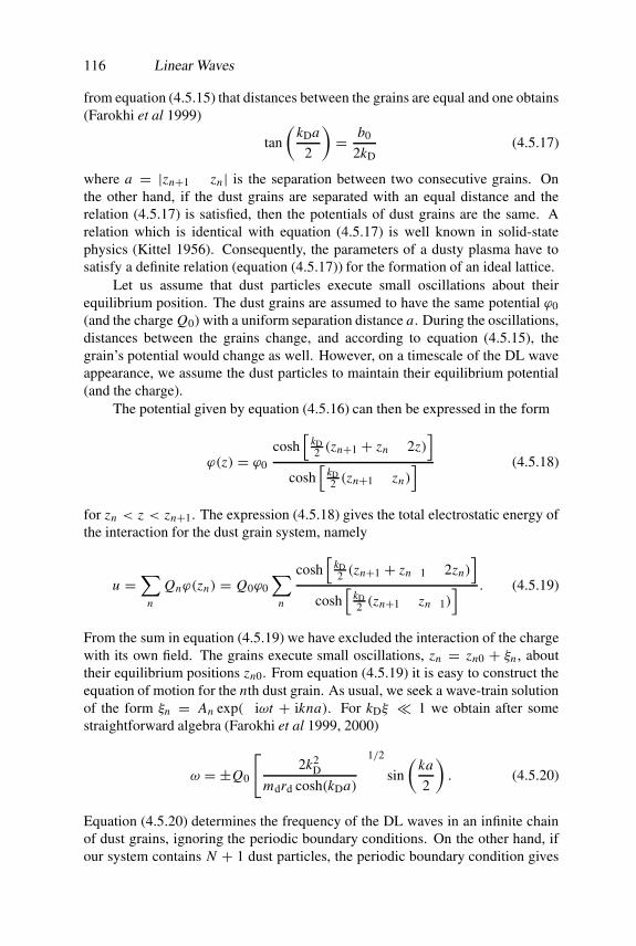
116 Linear Waves
from equation (4.5.15) that distances between the grains are equal and one obtains(Farokhi et al 1999)
tan
(kDa
2
)= b0
2kD(4.5.17)
where a = |zn+1 − zn | is the separation between two consecutive grains. Onthe other hand, if the dust grains are separated with an equal distance and therelation (4.5.17) is satisfied, then the potentials of dust grains are the same. Arelation which is identical with equation (4.5.17) is well known in solid-statephysics (Kittel 1956). Consequently, the parameters of a dusty plasma have tosatisfy a definite relation (equation (4.5.17)) for the formation of an ideal lattice.
Let us assume that dust particles execute small oscillations about theirequilibrium position. The dust grains are assumed to have the same potential ϕ0(and the charge Q0) with a uniform separation distance a. During the oscillations,distances between the grains change, and according to equation (4.5.15), thegrain’s potential would change as well. However, on a timescale of the DL waveappearance, we assume the dust particles to maintain their equilibrium potential(and the charge).
The potential given by equation (4.5.16) can then be expressed in the form
ϕ(z) = ϕ0
cosh[
kD2 (zn+1 + zn − 2z)
]cosh
[kD2 (zn+1 − zn)
] (4.5.18)
for zn < z < zn+1. The expression (4.5.18) gives the total electrostatic energy ofthe interaction for the dust grain system, namely
u =∑
n
Qnϕ(zn) = Q0ϕ0
∑n
cosh[
kD2 (zn+1 + zn−1 − 2zn)
]cosh
[kD2 (zn+1 − zn−1)
] . (4.5.19)
From the sum in equation (4.5.19) we have excluded the interaction of the chargewith its own field. The grains execute small oscillations, zn = zn0 + ξn , abouttheir equilibrium positions zn0. From equation (4.5.19) it is easy to construct theequation of motion for the nth dust grain. As usual, we seek a wave-train solutionof the form ξn = An exp(−iωt + ikna). For kDξ � 1 we obtain after somestraightforward algebra (Farokhi et al 1999, 2000)
ω = ±Q0
[2k2
D
mdrd cosh(kDa)
]1/2
sin
(ka
2
). (4.5.20)
Equation (4.5.20) determines the frequency of the DL waves in an infinite chainof dust grains, ignoring the periodic boundary conditions. On the other hand, ifour system contains N + 1 dust particles, the periodic boundary condition gives

Waves in Uniform Magnetoplasmas 117
the following N different frequencies for the first Brillouin zone
ω = ±Q0
[2k2
D
mdrd cosh(kDa)
]1/2
sin(πm
N
)(4.5.21)
for m = 1, 2, 3, . . . , N/2. According to equation (4.5.21) the maximumfrequency is given by
ωm = ±Q0
[2k2
D
mdrd cosh(kDa)
]1/2
. (4.5.22)
Expressions (4.5.20) and (4.5.22) differ from the expression found byMelandsø (1996), where the expression for the frequency includes also thepolynomial dependence on the parameter kDa. For kDa � 1 equation (4.5.20)gives
ω = ±Q0
(2k2
D
mdrd
)1/2
sin
(ka
2
). (4.5.23)
4.6 Waves in Uniform Magnetoplasmas
It is well known that the presence of an external magnetic field significantlymodifies the dispersion properties of both the electrostatic and electromagneticwaves in an electron–ion plasma. Thus, we focus our attention on low-frequency(in comparison with the electron gyrofrequency) electrostatic and electromagneticwaves in a weakly coupled dusty magnetoplasma.
4.6.1 Electrostatic waves
The dispersion properties of electrostatic plasma waves in a dusty plasmaare obtained by Fourier analysing the Vlasov and Poisson equations that aresupplemented by the dust charging equation. However, the latter is rather complexwhen an external magnetic field B0 z is present. Thus, to avoid the mathematicalcomplexities, we neglect the effects of dust charge fluctuations without losingany physical insight. The dusty plasma wave response in the electrostatic wavepotential φ is then deduced from
ε(ω, k) = 1+∑
s=e,i,d
χs = 0 (4.6.1)
where the dielectric susceptibility χs reads (Stenflo 1981)
χs =ω2
ps
k2V 2Ts
(1− ω
∞∑n=−∞
�n
∫ ∞
∞Fz dvz
ω − kzvz − nωcs
). (4.6.2)
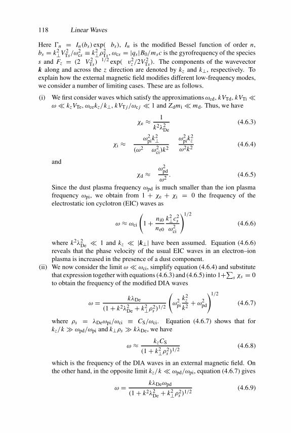
118 Linear Waves
Here �n = In(bs) exp(−bs), In is the modified Bessel function of order n,bs = k2⊥V 2
Ts/ω2cs ≡ k2⊥ρ2
Ts , ωcs = |qs |B0/msc is the gyrofrequency of the speciess and Fz = (2πV 2
Ts)−1/2 exp(−v2
z /2V 2Ts). The components of the wavevector
k along and across the z direction are denoted by kz and k⊥, respectively. Toexplain how the external magnetic field modifies different low-frequency modes,we consider a number of limiting cases. These are as follows.
(i) We first consider waves which satisfy the approximationsωcd, kVTd, kVTi �ω � kzVTe, ωcekz/k⊥, kVT j/ωc j � 1 and Zdmi � md. Thus, we have
χe ≈ 1
k2λ2De
(4.6.3)
χi ≈ −ω2
pik2⊥
(ω2 − ω2ci)k
2− ω2
pik2z
ω2k2(4.6.4)
and
χd ≈ −ω2
pd
ω2 . (4.6.5)
Since the dust plasma frequency ωpd is much smaller than the ion plasmafrequency ωpi, we obtain from 1 + χe + χi = 0 the frequency of theelectrostatic ion cyclotron (EIC) waves as
ω ≈ ωci
(1+ ni0
ne0
k2⊥c2s
ω2ci
)1/2
(4.6.6)
where k2λ2De � 1 and kz � |k⊥| have been assumed. Equation (4.6.6)
reveals that the phase velocity of the usual EIC waves in an electron–ionplasma is increased in the presence of a dust component.
(ii) We now consider the limit ω � ωci, simplify equation (4.6.4) and substitutethat expression together with equations (4.6.3) and (4.6.5) into 1+∑s χs = 0to obtain the frequency of the modified DIA waves
ω = kλDe
(1+ k2λ2De + k2⊥ρ2
s )1/2
(ω2
pik2
z
k2+ ω2
pd
)1/2
(4.6.7)
where ρs = λDeωpi/ωci ≡ CS/ωci. Equation (4.6.7) shows that forkz/k � ωpd/ωpi and k⊥ρs � kλDe, we have
ω ≈ kzCS
(1+ k2⊥ρ2s )
1/2(4.6.8)
which is the frequency of the DIA waves in an external magnetic field. Onthe other hand, in the opposite limit kz/k � ωpd/ωpi, equation (4.6.7) gives
ω = kλDeωpd
(1+ k2λ2De + k2⊥ρ2
s )1/2
(4.6.9)
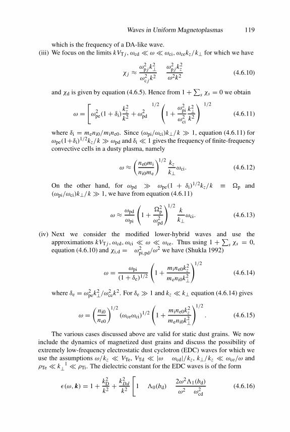
Waves in Uniform Magnetoplasmas 119
which is the frequency of a DA-like wave.(iii) We focus on the limits kVT j , ωcd � ω � ωci, ωcekz/k⊥ for which we have
χ j ≈ω2
p j k2⊥
ω2c j k
2− ω2
p j k2z
ω2k2(4.6.10)
and χd is given by equation (4.6.5). Hence from 1+∑s χs = 0 we obtain
ω =[ω2
pe(1+ δi)k2
z
k2 + ω2pd
]1/2 (1+ ω2
pi
ω2ci
k2⊥k2
)−1/2
(4.6.11)
where δi = meni0/mine0. Since (ωpi/ωci)k⊥/k � 1, equation (4.6.11) forωpe(1+δi)
1/2kz/k � ωpd and δi � 1 gives the frequency of finite-frequencyconvective cells in a dusty plasma, namely
ω ≈(
ne0mi
ni0me
)1/2 kz
k⊥ωci. (4.6.12)
On the other hand, for ωpd � ωpe(1 + δi)1/2kz/k ≡ �p and
(ωpi/ωci)k⊥/k � 1, we have from equation (4.6.11)
ω ≈ ωpd
ωpi
(1+ �2
p
ω2pd
)1/2k
k⊥ωci. (4.6.13)
(iv) Next we consider the modified lower-hybrid waves and use theapproximations kVT j , ωcd, ωci � ω � ωce. Thus using 1 +∑s χs = 0,equation (4.6.10) and χi,d = −ω2
pi,pd/ω2 we have (Shukla 1992)
ω = ωpi
(1+ δe)1/2
(1+ mine0k2
z
meni0k2⊥
)1/2
(4.6.14)
where δe = ω2pek2⊥/ω2
cek2. For δe � 1 and kz � k⊥ equation (4.6.14) gives
ω =(
ni0
ne0
)1/2
(ωceωci)1/2
(1+ mine0k2
z
meni0k2⊥
)1/2
. (4.6.15)
The various cases discussed above are valid for static dust grains. We nowinclude the dynamics of magnetized dust grains and discuss the possibility ofextremely low-frequency electrostatic dust cyclotron (EDC) waves for which weuse the assumptions ω/kz � VTe, VTd � |ω − ωcd|/kz , k⊥/kz � ωce/ω andρTe � k−1
⊥ � ρTi. The dielectric constant for the EDC waves is of the form
ε(ω, k) = 1+ k2D
k2 +k2
Dd
k2
[1−'0(bd)− 2ω2'1(bd)
ω2 − ω2cd
](4.6.16)
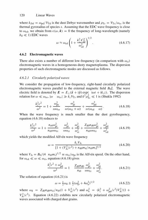
120 Linear Waves
where kDd = ωpd/VTd is the dust Debye wavenumber and ρTs = VTs/ωcs is thethermal gyroradius of species s. Assuming that the EDC wave frequency is closeto ωcd, we obtain from ε(ω, k) = 0 the frequency of long-wavelength (namelybd � 1) EDC waves
ω ≈ ωcd
(1+ k2⊥C2
D
ω2cd
)1/2
. (4.6.17)
4.6.2 Electromagnetic waves
There also exists a number of different low-frequency (in comparison with ωci)electromagnetic waves in a homogeneous dusty magnetoplasma. The dispersionproperties of such electromagnetic modes are discussed as follows.
4.6.2.1 Circularly polarized waves
We consider the propagation of low-frequency, right-hand circularly polarizedelectromagnetic waves parallel to the external magnetic field B0 z. The waveelectric field is denoted by E = E⊥(x + i y) exp(−iωt + ikzz). The dispersionrelation for ω � ωce, |ω − ωcs | � kzVTs and k2ρ2
Ts � 1 is (Shukla 1992)
k2z c2
ω2= 1+ ω2
pe
ωωce− ω2
pi
ω(ωci + ω)+ ω2
pd
ω(ωcd − ω). (4.6.18)
When the wave frequency is much smaller than the dust gyrofrequency,equation (4.6.18) reduces to
k2z c2
ω2 = 1+ ne0ω2pi
ni0ωωci− ω2
pi
ωωci+ ω2
pi
ω2ci
+ Zd0nd0ω2pi
ni0ωωci+ ω2
pd
ω2cd
(4.6.19)
which yields the modified Alfven wave frequency
ω = kzVA
[1+ (V 2A/c2)+ nd0md/ni0mi]1/2
(4.6.20)
where VA = B0/(4πni0mi)1/2 ≡ ωci/ωpi is the Alfven speed. On the other hand,
for ωcd � ω � ωci, equation (4.6.18) gives
k2z c2 + ω2
pd
ω2= 1− Zd0nd0
ni0
ω2pi
ωωci+ ω2
pi
ω2ci
. (4.6.21)
The solution of equation (4.6.21) is
ω = 12ωd ± 1
2 (ω2D + 4ω2
a)1/2 (4.6.22)
where ωd = Zd0nd0ωci/ni0(1 + V 2A/c2) and ω2
a = (k2z + ω2
pd/c2)V 2A/(1 +
V 2A/c2). Equation (4.6.22) exhibits new circularly polarized electromagnetic
waves associated with charged dust grains.
Waves in Uniform Magnetoplasmas 121
4.6.2.2 Mixed modes: dynamic dust
The properties of mixed modes are described by the magnetohydrodynamic(MHD) equations of dusty plasmas for the case in which the dust inertia playsan important role (Shukla and Rahman 1996, Birk et al 1996). The dynamics oflow-frequency (in comparison with the ion gyrofrequency) electromagnetic wavesin our dusty plasma is governed by the dust continuity equation
∂nd
∂ t+ ∇ · (ndvd) = 0 (4.6.23)
the inertial dust momentum equation
mdnd
(∂
∂ t+ vd ·∇
)vd = −Zd0nde
(E + 1
cvd × B
)−∇ pd (4.6.24)
the inertialess ion momentum equation
0 = nie
(E + 1
cvi × B
)−∇ pi (4.6.25)
the inertialess electron momentum equation
0 = −nee
(E + 1
cve × B
)−∇ pe (4.6.26)
Faraday’s law∂B∂ t= −c∇ × E (4.6.27)
Ampere’s law
∇ × B = 4πe
c(nivi − neve − Zd0ndvd) ≡ 4π
cJ (4.6.28)
together with ∇ · B = 0 and the electron and ion continuity equations. Hereps = nskBTs is the pressure and E and B are the electric and magneticfields, respectively. Furthermore, in equation (4.6.28) we have neglected thedisplacement current as we are concerned with electromagnetic waves whosephase velocity is much smaller than the speed of light. We have also assumedZd0/md to be uniform. Adding equations (4.6.24)–(4.6.26) and making use ofequation (4.6.28) we obtain
mdnd
(∂
∂ t+ vd · ∇
)vd = −∇
(P + B2
8π
)+ 1
4π(B ·∇)B (4.6.29)
where P = ∑s ps ≡ ndkB(Td + Zd0Ti) + nekB(Te + Ti). Eliminating E fromequations (4.6.24) and (4.6.27) we have
∂B∂ t= ∇ × (vd × B)+ ckB
Zd0en2d
∇nd × ∇Td + md
Zd0e∇ ×
[(∂
∂ t+ vd · ∇
)vd
].
(4.6.30)
122 Linear Waves
Equations (4.6.23), (4.6.29) and (4.6.30) are the desired MHD equations for adusty magnetoplasma in which the dust inertia dominates. They govern thedynamics of various low-frequency electromagnetic waves in a magnetized dustyplasma. In order to study these waves, we Fourier transform equations (4.6.23),(4.6.29) and (4.6.30) by letting nd = nd0 + nd1 and B = B0 z + B1, wherend1 � nd0, B1 � B0 z and ne0(Te+ Ti)� nd0(Td+ Zd0Ti). Combining Fourier-transformed equations (4.6.23), (4.6.29) and (4.6.30), we obtain the dispersionrelation (Shukla and Rahman 1996)
(ω2 − ω2DA)Dm(ω, k) = ω2
DA
ω2cd
ω2k2V 2A(ω
2 − k2V 2da) (4.6.31)
where ωDA = kzVDA is the dust-Alfven frequency
Dm(ω, k) = ω4 − ω2k2(V 2DA + V 2
da)+ ω2DAk2V 2
da (4.6.32)
VDA = B0/(4πnd0md)1/2 is the dust Alfven speed and Vda = [(Zd0kBTi +
kBTd)/md]1/2 is the modified DA speed. We note that the dust-Alfven and DAspeeds are inversely proportional to m1/2
d , indicating that the dust inertia playsa major role in the wave dynamics. Equation (4.6.31), which exhibits a linearcoupling between various dusty plasma modes, is a sixth-order polynomial in ω
and can be readily analysed numerically. However, some interesting analyticalresults follow in several limiting cases, which are presented below.
(i) Perpendicular propagation (kz = 0)
We first consider flute perturbations (kz = 0) for which equation (4.6.31) gives(Rao 1993)
ω = k⊥(V 2DA + V 2
da)1/2 (4.6.33)
which is the frequency of the dust-magnetosonic waves.
(ii) Parallel propagation (k⊥ = 0)
For the wave propagation along the external magnetic field lines, we obtain fromequation (4.6.31)
k2z V 2
DA =ω2ωcd
(ωcd ∓ ω)(4.6.34)
which is the dispersion relation for coupled dust cyclotron and dust-Alfven waves.For ω � ωcd equation (4.6.34) gives the dispersive dust-Alfven wave frequency
ω ≈ kzVDA
(1± kzVDA
2ωcd
). (4.6.35)

Waves in Non-uniform Magnetoplasmas 123
On the other hand, in the limit ω � ωcd, equation (4.6.34) reduces to
ω ≈ k2z V 2
DA
ωcd≡ k2
z c2ωcd
ω2pd
(4.6.36)
which is the dust whistler frequency.
(iii) Oblique propagation
We use the approximations kz/k � 1 and ω/k⊥ � Vda � VDA inequation (4.6.31) and obtain the dispersion relation for the shear dust Alfvenwaves as
ω ≈ kz VDA(1+ k2⊥ρ2a )
1/2 (4.6.37)
where ρa = Vda/ωcd. Furthermore, for ω � kzVDA and Vda � VDA,equation (4.6.31) yields
(ω2 − k2z V 2
da) =ω2
ω2cd
(ω2 − k2V 2da) (4.6.38)
which exhibits a coupling between the modified DA and dust cyclotron waves.When ω ∼ kzVda, we have from equation (4.6.38)
ω ≈ kzVda
(1+ k2⊥ρ2a )
1/2(4.6.39)
which is the frequency of the dispersive DA waves in a magnetized dusty plasma.
4.7 Waves in Non-uniform Magnetoplasmas
It is well established that all plasma systems, especially dusty plasma systems,always contain some region of inhomogeneity capable of causing drift motionsand associated waves in a magnetized dusty plasma. Thus, we consider herea non-uniform dusty magnetoplasma containing immobile dust grains and theequilibrium density gradient ∂ns0/∂x (unperturbed plasma number densitiesns0(x) are assumed to be inhomogeneous along the x-axis) and study thedispersion properties of low-frequency (in comparison withωci), long-wavelength(in comparison with the ion gyroradius) electrostatic and electromagnetic waves.The external magnetic field zB0 is along the z-axis. The quasi-neutrality conditionat equilibrium is given by equation (4.4.1). In the electric field (E⊥ = −∇⊥φ) oflow-frequency waves, the perpendicular components of the electron and ion fluidvelocities are (Weiland 2000)
ve⊥ ≈ c
B0z ×∇⊥φ − ckBTe
eB0ne0z ×∇⊥ne1 (4.7.1)

124 Linear Waves
and
vi⊥ ≈ c
B0z ×∇⊥φ + ckBTi
eB0ni0z ×∇ni1 − c
B0ωci
(∂
∂ t+ ui∗ ·∇
)∇⊥φ (4.7.2)
where ui∗ = (ckBTi/eB0ni0) z×∇ni0(x) is the unperturbed ion diamagnetic driftvelocity.
4.7.1 Electrostatic waves
We first consider propagation of coupled convective cells and dust drift-acousticwaves. Accordingly, we substitute equation (4.7.1) into the electron continuityequation and obtain
∂ne1
∂ t+ c
B0z ×∇φ ·∇ne0 + ne0
∂vez
∂z= 0 (4.7.3)
where the parallel (to z) component of the electron fluid velocity vez is determinedby
∂vez
∂ t= e
me
∂
∂z
(φ − kBTe
ene0
∂ne1
∂z
). (4.7.4)
Next, we substitute equations (4.7.1) and (4.7.2) into the charge conservationequation
∇ · (eni0vi − ene0ve) = 0 (4.7.5)
by imposing the quasi-neutrality approximation (ne1 ≈ ni1), which is valid for adense plasma in which ωpi � ωci. We obtain
∂∇2⊥φ∂ t
+ ω2ci
ω2pi
4πc
B0z×∇(qd0nd0) ·∇φ− B0ωci
c
∂
∂z
(viz − ne0
ni0vez
)= 0 (4.7.6)
where the parallel component of the ion fluid velocity perturbation viz isdetermined from
∂viz
∂ t= − e
mi
∂
∂z
(φ + 3kBTini1
eni0
). (4.7.7)
Equations (4.7.3)–(4.7.7) are the desired equations for studying coupledconvective cells and dust drift-ion acoustic waves in a dusty magnetoplasma. Wenow consider two limiting cases.
(i) |∂/∂ t| � VTe|∂/∂z|Using |∂/∂ t| � VTe∂/∂z and ignoring the parallel ion dynamics, we have fromequations (4.7.4) and (4.7.6)
∂vez
∂ t= e
me
∂φ
∂z(4.7.8)
Waves in Non-uniform Magnetoplasmas 125
and
∂∇2⊥φ∂ t
+ ω2ci
ω2pi
4πc
B0z ×∇(qd0nd0) ·∇φ + ne0 B0ωci
ni0c
∂vez
∂z= 0. (4.7.9)
Assuming that vez and φ are proportional to exp(−iωt + ik · r), we obtain fromequations (4.7.8) and (4.7.9) the linear dispersion relation (Mamun and Shukla2000) for coupled modified convective cells and the Shukla–Varma (SV) mode(Shukla and Varma 1993)
ω = ωsv ± 12 (ω
2sv + 4ω2
cc)1/2 (4.7.10)
where
ωsv = −4πcω2ciky∂(qd0nd0)/∂x
B0k2⊥ω2pi
(4.7.11)
is the SV frequency (Shukla and Varma 1993) and
ωcc =(
ne0
ni0
)1/2
(ωceωci)1/2 kz
k⊥(4.7.12)
is the modified convective cell frequency (Okuda and Dawson 1973). We notethat in a uniform plasma, the SV mode disappears.
(ii) |∂/∂ t| � VTe|∂/∂z|We consider coupled drift-DIA waves in the approximation |∂/∂ t| � VTe|∂/∂z|.Here the inertialess electrons rapidly thermalize along the z direction and thecorresponding electron number density perturbation is given by the Boltzmannrelation
ne1 ≈ ne0(x)eφ
kBTe(4.7.13)
which follows from equation (4.7.4). Invoking the quasi-neutrality approximationni1 = ne1, we can substitute equation (4.7.13) into the ion continuity equation toobtain
∂
∂ t(φ − ρ2
s ∇2⊥φ)− ρ2s ωci z ×∇ ln ni0 ·∇φ + ni0kBTe
ne0e
∂viz
∂z= 0. (4.7.14)
By using equation (4.7.13) we can write equation (4.7.7) as
∂viz
∂ t= −
(1+ 3
ne0Ti
ni0Te
)e
mi
∂φ
∂z. (4.7.15)
Fourier transforming equations (4.7.14) and (4.7.15) and combining them, weobtain the dispersion relation (Shukla et al 1991)
ω = ω∗2(1+ k2
yρ2s )± 1
2
[ω2∗
(1+ k2yρ
2s )
2 + 4k2
z C2ss
1+ k2yρ
2s
]1/2
(4.7.16)

126 Linear Waves
where ω∗ = −(ckBTe/eB0ne0)ky∂ni0/∂x is the modified drift wave frequencyand Css = CS(1+ 3ne0Ti/ni0Te)
1/2. When ω∗ � kzCss equation (4.7.16) yields
ω = ω∗1+ k2⊥ρ2
s
(4.7.17)
which is the frequency of the dispersive dust drift waves.
4.7.2 Electromagnetic waves
To study electromagnetic waves that may exist in a non-uniform dustymagnetoplasma, we first consider different types of mixed modes (mixture ofelectrostatic and electromagnetic waves) and then a purely electromagnetic mode,namely a non-ducted dust whistler.
4.7.2.1 Mixed modes: static dust
We consider a low-β (β = 8πn0kBT/B20 � 1) plasma in which the parallel
component of the electron fluid velocity is determined by equation (4.6.28),yielding
vez ≈ c
4πne0e∇2⊥Az (4.7.18)
where Az is the parallel component of the vector potential. In obtainingequation (4.7.18) we set B = ∇Az × z and neglected the parallel componentsof the ion and dust current densities as well as the compressional magnetic fieldperturbation. Thus, the DIA and magnetosonic waves are decoupled in our low-βdusty plasma system. Substituting equations (4.7.1) and (4.7.18) into the electroncontinuity equation and letting n j = n j0(x)+ n j1, where n j1 � n j0, we obtain
∂ne1
∂ t− c
B0z ×∇ne0 ·∇φ + c
4πe
∂∇2⊥Az
∂z= 0. (4.7.19)
On the other hand, substitution of the ion fluid velocity (4.7.2) into the ioncontinuity equation yields
∂ni1
∂ t− c
B0z ×∇⊥ni0 ·∇⊥φ − cni0
B0ωci
(∂
∂ t+ ui∗ ·∇⊥
)∇2⊥φ = 0. (4.7.20)
Subtracting equation (4.7.20) from equation (4.7.19) and making use of Poisson’sequation (namely ∇2φ = 4πe(ne1 − ni1) for stationary dust grains), we obtainthe modified ion vorticity equation(
∂
∂ t+ ui0
∂
∂y
)∇2⊥φ +
V 2A
c2
∂∇2φ
∂ t+ ωciδdκd
∂φ
∂y+ V 2
A
c
∂∇2⊥Az
∂z= 0 (4.7.21)
where ui0 = (ckBTi/eB0ni0)∂ni0/∂x is the y component of the unperturbed iondiamagnetic drift velocity, δd = qd0nd0/eni0 and κd = ∂ ln[(qd0nd0(x)]/∂x .
Waves in Non-uniform Magnetoplasmas 127
By using equations (4.7.1) and (4.7.18), the parallel component of theelectron momentum equation can be written as
(∂
∂ t+ ue0
∂
∂y
)Az − λ2
e∂∇2⊥Az
∂ t+ c
∂
∂z
(φ − kBTe
e
ne1
ne0
)= 0 (4.7.22)
where ue0 = −(ckBTe/eB0ne0)∂ne0(x)/∂x is the y component of theunperturbed electron diamagnetic drift velocity and λe = c/ωpe is the electronskin depth.
Equations (4.7.19), (4.7.21) and (4.7.22) are the desired equationsfor the coupled drift-Alfven–Shukla–Varma modes in a non-uniform dustymagnetoplasma. The dispersion relation can be derived by supposing that ne1, φ
and Az are proportional to exp(−iωt + iky y + ikzz). Accordingly, in the localapproximation, when the wavelength is much smaller than the scalelength ofthe density gradient, we can Fourier transform equations (4.7.19), (4.7.21) and(4.7.22) and combine them to obtain the general dispersion relation (Pokhotelovet al 1999)
(ω2 − ωωm − ω2IAk2
yρ2s )(ω − ωi∗ − ωsv) = ω2
IA(ω − ωe∗) (4.7.23)
whereωm = ωe∗
(1+ k2yλ
2e)
(4.7.24)
is the magnetic drift wave frequency
ω j∗ = kyu j0 (4.7.25)
is the drift wave frequency and
ωIA = kzVA
(1+ k2yλ
2e)
1/2(4.7.26)
is the frequency of the inertial Alfven waves. In deriving equation (4.7.23) wehave assumed (k2/k2
y)ω2ci/ω
2pi � 1, where k2 = k2
y + k2z . We now examine
equation (4.7.23) in various limiting cases.
(i) ω j∗ = 0
For a homogeneous dusty plasma (namely ω j∗ = 0), equation (4.7.23) correctlyreproduces the frequency of the dispersive Alfven waves (Shukla and Stenflo1999). When the parallel phase velocity (ω/kz) of the dispersive Alfven wavesis much smaller than the electron thermal speed VTe, we can neglect the parallelelectron inertial effect (namely k2
yλ2e � 1) and obtain from (4.7.23)
ω = kzVA(1+ k2yρ
2s )
1/2 (4.7.27)

128 Linear Waves
which is the frequency of the dispersive kinetic Alfven waves in an intermediate-β (me/mi � β � 1) plasma. On the other hand, forω/kz � VTe, we can neglectthe parallel electron pressure gradient term (or the k2
yρ2s term in comparison with
unity), and obtain from equation (4.7.23)
ω = kzVA
(1+ k2yλ
2e)
1/2(4.7.28)
which is the frequency of the dispersive inertial Alfven waves in a very low-βplasma (β � me/mi).
(ii) ω � ωm, ω j∗
We observe from equation (4.7.23) that for ω � ωm, ω j∗ the dispersive Alfvenwaves are linearly coupled with the SV mode, ω = ωsv. Specifically, in acold (Tj → 0) dusty plasma with ω/kz � VTe and ω � ωi∗, we obtain fromequation (4.7.23)
ω2 − ωωsv − k2z V 2
A
1+ k2yλ
2e= 0 (4.7.29)
which clearly shows that the coupling between the SV mode and the inertialAlfven wave arises due to the parallel electron motion in the wave electric andmagnetic fields.
Furthermore, in the limit kyρs → 0 (or vanishing parallel electron pressuregradient force) and ωi∗ = 0, we obtain from equation (4.7.23)
[(1+ k2yλ
2e)ω − ωe∗](ω − ωsv)ω = k2
z V 2A(ω − ωe∗) (4.7.30)
which shows that the magnetostatic drift mode (ω = ωm), the SV mode (ω =ωsv), the inertial Alfven wave (ω = ωIA), and the electron drift mode (ω = ωe∗)are linearly coupled.
(iii) kzvez = 0
When the parallel electron motion is completely neglected (namely kzvez = 0),we see from equation (4.7.23) that the flute-like magnetostatic mode (ω = ωm)and the modified SV mode (ω = ωi∗ +ωsv) appear as independent normal modesof a non-uniform dusty magnetoplasma containing warm ions.
(iv) k2yλ
2e � 1
When the perpendicular wavelength is much larger than λe, we obtain fromequation (4.7.23) for ω � ωi∗
(ω2 − ωωsv − k2z V 2
A)(ω − ωe∗) = k2yρ
2s k2
z V 2A(ω − ωsv) (4.7.31)
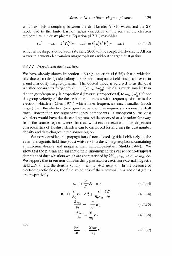
Waves in Non-uniform Magnetoplasmas 129
which exhibits a coupling between the drift-kinetic Alfven waves and the SVmode due to the finite Larmor radius correction of the ions at the electrontemperature in a dusty plasma. Equation (4.7.31) resembles
(ω2 − ωωi∗ − k2z V 2
A)(ω − ωe∗) = k2yρ
2s k2
z V 2A(ω − ωi∗) (4.7.32)
which is the dispersion relation (Weiland 2000) of the coupled drift-kinetic Alfvenwaves in a warm electron–ion magnetoplasma without charged dust grains.
4.7.2.2 Non-ducted dust whistlers
We have already shown in section 4.6 (e.g. equation (4.6.36)) that a whistler-like ducted mode (guided along the external magnetic field lines) can exist ina uniform dusty magnetoplasma. The ducted mode is referred to as the dustwhistler because its frequency (ω = k2
z c2ωcd/ω2pd), which is much smaller than
the ion gyrofrequency, is proportional (inversely proportional) to ωcd (ω2pd). Since
the group velocity of the dust whistlers increases with frequency, similar to theelectron whistlers (Chen 1974) which have frequencies much smaller (muchlarger) than the electron (ion) gyrofrequency, low-frequency components shalltravel slower than the higher-frequency components. Consequently, the dustwhistlers would have the descending tone while observed at a location far awayfrom the source region where the dust whistlers are excited. The dispersioncharacteristics of the dust whistlers can be employed for inferring the dust numberdensity and dust charges in the source region.
We now consider the propagation of non-ducted (guided obliquely to theexternal magnetic field lines) dust whistlers in a dusty magnetoplasma containingequilibrium density and magnetic field inhomogeneities (Shukla 1999). Weshow that the plasma and magnetic field inhomogeneities cause spatio-temporaldampings of dust whistlers which are characterized by kVT j , ωcd � ω � ωci, kc.We suppose that in our non-uniform dusty plasma there exist an external magneticfield zB0(x) and the density ni0(x) = ne0(x) + Zd0nd0(x). In the presence ofelectromagnetic fields, the fluid velocities of the electrons, ions and dust grainsare, respectively
ve⊥ ≈ c
B0E⊥ × z (4.7.33)
vi⊥ ≈ c
B0E⊥ × z + c
B0ωci
∂E⊥∂ t
(4.7.34)
∂vez
∂ t= − e
meEz (4.7.35)
∂viz
∂ t= e
miEz (4.7.36)
and∂vd
∂ t= − Zd0e
mdE (4.7.37)
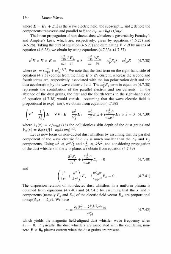
130 Linear Waves
where E = E⊥ + Ez z is the wave electric field, the subscript ⊥ and z denote thecomponents transverse and parallel to z and ωci = eB0(x)/mic.
The linear propagation of non-ducted dust whistlers is governed by Faraday’sand Ampere’s laws, which are, respectively, given by equations (4.6.27) and(4.6.28). Taking the curl of equation (4.6.27) and eliminating ∇× B by means ofequation (4.6.28), we obtain by using equations (4.7.33)–(4.7.37)
c2∇ ×∇ × E = −ω2pd
ωcd
∂E⊥∂ t
× z − ω2pi
ωci
∂E⊥∂ t
− ω2p Ez z − ω2
pd E (4.7.38)
where ωp = (ω2pe + ω2
pi)1/2. We note that the first term on the right-hand side of
equation (4.7.38) comes from the finite E × B0 current, whereas the second andfourth terms are, respectively, associated with the ion polarization drift and thedust acceleration by the wave electric field. The ω2
p Ez term in equation (4.7.38)represents the contribution of the parallel electron and ion currents. In theabsence of the dust grains, the first and the fourth terms in the right-hand sideof equation (4.7.38) would vanish. Assuming that the wave electric field isproportional to exp(−iωt), we obtain from equation (4.7.38)(
∇2 − 1
λ2d
)E − ∇∇ · E − ω2
V 2A
E⊥ −ω2
p
c2Ez z + i
ω2pdω
ωcdc2E⊥ × z = 0 (4.7.39)
where λd(x) = c/ωpd(x) is the collisionless skin depth of the dust grains andVA(x) = B0(x)/[4πni0(x)mi]1/2.
Let us now focus on non-ducted dust whistlers by assuming that the parallelcomponent of the wave electric field Ez is much smaller than the Ex and Ey
components. Using ω2 � k2V 2A and ω2
pd � k2c2, and considering propagationof the dust whistlers in the x–z plane, we obtain from equation (4.7.39)
∂2 Ex
∂z2+ i
ω2pdω
ωcdc2Ey = 0 (4.7.40)
and (∂2
∂x2+ ∂2
∂z2
)Ey − i
ω2pdω
ωcdc2Ex = 0. (4.7.41)
The dispersion relation of non-ducted dust whistlers in a uniform plasma isobtained from equations (4.7.40) and (4.7.41) by assuming that the x and ycomponents (namely Ex and Ey) of the electric field vector E⊥ are proportionalto exp(ikx x + ikzz). We have
ω = kz(k2z + k2
x)1/2c2ωcd
ω2pd
(4.7.42)
which yields the magnetic field-aligned dust whistler wave frequency whenkx = 0. Physically, the dust whistlers are associated with the oscillating non-zero E × B0 plasma current when the dust grains are present.

Waves in Non-uniform Magnetoplasmas 131
However, in a non-uniform dusty plasma the electric field components Ex
and Ey may vary as Ex (x) exp(ikzz) and Ey(x) exp(ikzz). Furthermore, forour purposes, the equilibrium density nd0(x) and magnetic field B0 have typicalprofiles of the form n0(1 + x/Ln) and B0(1 + x/LB), where Ln and LB are thescale sizes of the density and magnetic field inhomogeneities, respectively. Thus,equations (4.7.40) and (4.7.41) can be combined to yield
∂2 Ex
∂x2 + λ1 Ex + λ2x Ex + λ3x2 Ex = 0 (4.7.43)
where λ1 = k2z (ω
2 −ω2w)/ω
2w, λ2 = 2ω2k2
z (kn − kb)/ω2w, λ3 = (ω2k2
z /ω2w)(k
2n −
k2b − 4knkb), kn = ∂ ln nd0/∂x ≡ L−1
n , and kb = ∂ ln B0/∂x ≡ L−1B . The
frequency of the ducted dust whistler is defined as ωw = k2z c2ωcd/ω
2pd, where ωcd
and ωpd are the values of the dust gyro and dust plasma frequencies at x = 0. Wehave assumed that |x | � |Ln |, |LB|. It is seen that for λ3 < 0 the solution ofequation (4.7.43) is bounded and is (for large |x |)
Ex = E0 exp
[−√|λ3|
2(x − x0)
2]
(4.7.44)
where x0 = λ2/2|λ3|. The dust whistlers would not propagate and are damped.On the other hand, for λ3 > 0, equation (4.7.43) has for large |x | the solution
Ex = E0 exp
[−√λ3
2(x + x0)
2]
(4.7.45)
which indicates that non-localized non-ducted whistlers would carry energyoutwards and are damped.
We now consider the propagation of non-ducted dust whistlers in thepresence of a uniform external magnetic field and a parabolic density profile ofthe form nd0 = nd0(1 − x2/L2
n). Here equation (4.7.43) for x2 � L2n is replaced
by a parabolic cylinder equation
∂2 Ex
∂x2+ λ1 Ex − λ4x2 Ex = 0 (4.7.46)
where λ4 = ω2k2z k2
n/2ω2w. The eigenfunction solutions of equation (4.7.46) with
outgoing wave boundary conditions are
Ex = Hn(√σ x) exp(−σ x2/2) (4.7.47)
where σ = √λ4, Hn are the Hermite polynomials and n = 0, 1, 2. We note thatthe eigenfunction decays exponentially with x2, so that the width of the mode canbe approximated by 2/λ1/4
4 .
132 Linear Waves
Figure 4.2. Schematic illustration of the experimental set-up for producing a confineddusty plasma where the DA waves are observed (after Thompson et al 1999).
4.8 Experimental Observations
We have described different types of waves/modes that are theoretically found toexist in unmagnetized and magnetized dusty plasmas. Recently, some of thesewaves, namely the DA waves, the DIA waves and the DL waves have also beenobserved in laboratory experiments (Barkan et al 1995a, 1996, D’Angelo et al1996, Pieper and Goree 1996, Morfill et al 1997, Homann et al 1997, Thompsonet al 1999, Thomas and Watson 2000). This section is concerned with theexcitation of these waves in laboratory experiments.
4.8.1 Dust acoustic waves
The low-frequency DA waves have been observed (Barkan et al 1995a, Thompsonet al 1999) by using the experimental set-up schematically shown in figure 4.2.The potassium plasma column of a Q-machine was surrounded over its endportion (∼30 cm in length) by a rotating dust dispenser that continuallyrecycled the dust particles (kaolin). The average grain size was around 5 µm(approximately 90% of the dust grains had sizes in between 1 and 15 µm). Thelifetime of the dust grain in the plasma column was around 0.1 s. The DA waveswith periods comparable to or longer than 0.1 s could not evidently be studiedin this device. So a suitable modification was made by using an anode doublelayer (shown in figure 4.2) to trap and confine the negatively charged dust grainsin the Q-machine for much longer times. A neutral gas (generally nitrogen ata pressure of 60–80 mTorr was introduced into the device and a bias voltage(∼200 V) was applied to a small anode disc (of ∼1.6 cm diameter) located nearthe far end of the plasma column. This produces a cylindrical double layer (fire-rod) within which the space potential is ∼55 V that is above the space potentialof the surrounding K+-electron plasma. Thus, negatively charged dust grains can

Experimental Observations 133
Figure 4.3. A typical single-frame image of a DA wave pattern recorded in the videocamera (after Thompson et al 1999).
be indefinitely trapped within the fire-rod, provided their mass is not too large.Not only at the edges of the fire-rod but also within it there exists an electricfield which (on axis) is directed away from the disc electrode and has an averagemagnitude of �1 V cm−1. Under these conditions, the DA waves are observedthrough a side port, within the dust-loaded fire-rod. The waves appear as soonas the kaolin dust is introduced into the fire-rod. The observations were madeby using a simple flashlight and a video camera. A typical wave pattern with awavelength of ∼0.6 cm is shown in figure 4.3.
The speed with which the pattern moved from right to left away from thedisc electrode towards the Q-machine hot plate was measured from a successionof such pictures. A characteristic plot of the position of some given wave featureversus time of arrival yields a propagation speed of ∼9 cm s−1 (Barkan et al1995a). The frequency of the wave with a wavelength of 0.6 cm and a speed of9 cm s−1 turns out to be 15 Hz. The other parameters used for this experiment(Barkan et al 1995a) are nd/ne � 10−4, Zd � 4 × 10⁴ and md � 10−9 g. Forthe parameters of Barkan et al (1995a) one finds that equation (4.2.11) yieldsa DA wave frequency (Rao et al 1990) which is in perfect agreement with theexperimentally observed value.

134 Linear Waves
Figure 4.4. The variation of the quantity Vp(η)/Vp(1) with η (after Barkan et al 1996),where η = ne0/ni0. The theoretical results (based on fluid model) correspond to v0 = cs ,where v0 (cs ) is the plasma drift (ion-acoustic) speed.
4.8.2 Dust ion-acoustic waves
DIA waves have been experimentally excited (Barkan et al 1996, Merlino etal 1998) by means of a grid inserted into the plasma column produced in a Q-machine as shown in figure 1.8. A fully ionized, magnetized (B0 ≤ 4.0× 10³ G)potassium plasma column of a Q-machine was surrounded over its end portion(∼30 cm in length) by a rotating dust dispenser that continually recycled the dustparticles (kaolin). The grid was placed perpendicular to the magnetic field andapproximately 3 cm upstream from the dust dispenser.
The grid was biased at several volts negative with respect to the space chargepotential and a tone-burst sinusoidal voltage signal of frequency 20–80 kHz andamplitude 4–5 V peak to peak was applied to it. This produced near the grida density perturbation which then travelled down the column, into the region ofthe dust dispenser, as the DIA waves. By means of an axially moveable Langmuirprobe (a disc of 1 cm in diameter) the phase and amplitude measurements could beperformed at various axial locations and the wave phase speed Vp, the wavelengthλ and the attenuation length λa were determined with (η < 1) and without(η = 1) the dust. The quantity Vp(η)/Vp(1) is plotted as a function of η infigure 4.4. The other parameters for this experiment (Barkan et al 1996) areni � ne � 106 cm−3, Te � Ti � 2320 K, rd � 5 µm and md � 10−9 g.As the wavelength corresponding to these plasma parameters (the number densityand the temperature) is ∼0.3 cm, the launcher grid had to have the rather unusualfeature of an inter-wire spacing of ∼0.5 cm in order to obtain an appropriatedensity modulation by the applied sinusoidal voltage. A further condition that
Experimental Observations 135
Figure 4.5. The experimental set-up for the observation of laser excited DL waves (afterHomann et al 1997).
the ion gyroradius is comparable to or larger than the grid wire spacing requiredthat the magnetic field is not much above 1000 G at which the gyroradius of0.2 eV K+ ions is ∼0.3 cm. It is obvious from figure 4.4 that (i) the DIA waveis indeed a normal mode in a dusty plasma and (ii) the phase speed of the DIAwave increases when η < 1. The experimental observations of enhanced phasespeed and reduced damping of the DIA waves are consistent with the theoreticalprediction of Shukla and Silin (1992).
4.8.3 Dust lattice waves
DL waves have been experimentally observed by Morfill et al (1997) and Homannet al (1997). The experimental arrangements of the latter are shown in figure 4.5.The dust particles are trapped in the lower sheath of a parallel plate. The upperelectrode is grounded and the lower one is powered at a frequency of 13.56 MHzand a rf power of 7 W. To arrange the dust grains in a linear chain, a rectangularbarrier of 4 mm height and x = 90 mm × y = 20 mm inner spacing is put

136 Linear Waves
Figure 4.6. The sequences of 15 snapshots for a linear chain arrangement of 10 particles.
on the lower electrode (as shown in figure 4.5). In this experiment a dozenof mono-disperse spherical melamine formaldehyde plastic particles of radiusrd = (4.75 ± 0.15) µm and mass density ρd = 1.514 g cm−3 are insertedinto the plasma chamber. These particles arrange in a linear chain with aninterparticle distance of a = 930 µm at a gas pressure of 22 Pa. The particlesare illuminated by a horizontally expanded thin laser sheet for observation. Thewhole arrangement is viewed in scattered light from the top with a video camera.The beam (20 mW, 690 nm) of a laser diode is focused on the first particle.The laser’s radiation pressure pushes the first particle, thus exciting the chain.Although the focus diameter is larger than the particle diameter, the particle mustbe close to the inner focus to be moved by the laser. The other particles arein the defocused region and are, therefore, almost unaffected by the beam. Thelaser diode is switched on and off by a transistor–transistor–logic (TTL) signal.The switching frequency of the TTL signal used in the experiment of Homann etal (1997) was varied between 0.4 and 3 Hz with a constant duty cycle of 50%.

Experimental Observations 137
The mechanism of the excitation is mainly attributed to the radiation pressure.Homann et al (1997) used a 20 mW laser for which the radiation pressure force isof the order of or smaller than the gravitational force and electrostatic field force,but much larger than all other related forces (e.g. thermophoretic force). Becauseof the narrow width of the potential well in the y direction (due to the barrier)and z direction due to the balance of the gravitational force and the electrostaticfield force, the dust particles can only move in the x direction. An impressionof their oscillatory motion, whose dispersion relation (equation (4.5.6)) can bedescribed by that of the LDL waves, is shown in figure 4.6. It shows a series ofvideo images at the frequency of 1.3 Hz and at a pressure of 22 Pa. The time-step between each video image is 100 ms. It is clearly seen that only the firstparticle (the rightmost particle which is seen by the bright spot of scattered light)is pushed by the exciting laser. It should be noted that the exciting laser was onfor images 2–5 and 10–13 and was off in the other images.

Chapter 5
Instabilities
5.1 Introduction
We have discussed in chapter 4 the properties of electrostatic and electromagneticwaves in dusty plasmas near thermodynamical equilibrium. The normal wavemodes represent stable elementary excitations. The collective modes suffera certain amount of collisional and non-collisional (Landau and dust chargefluctuation induced) damping.
However, most dusty plasmas in space and laboratories are far fromthermodynamic equilibrium. A non-equilibrium plasma is characterized by thepresence of unstable collective modes whose amplitudes grow exponentially.There are several mechanisms by which the plasma waves can be driven at non-thermal levels when free energy sources are available in our dusty plasma system.For example, dusty plasmas can be subjected to the influence of external forcefields which create flows of particles, momentum and energy. Furthermore, thespatial variation of the physical quantities, such as the pressure, the intensity ofthe dc electric and magnetic fields, the plasma flow velocity and the dust graincharge, are involved in laboratory and space plasmas. The energies of laser/radarbeams and radio-frequency waves can also be coupled to normal modes of dustyplasmas.
There are new classes of instabilities associated with the ion drag force,ionization, dust charge gradient, etc in dusty plasmas, besides the usualBuneman, Kelvin–Helmholtz, Rayleigh–Taylor, pressure gradient and parametric(stimulated scattering) instabilities. The studies of instabilities are of greatimportance because they are helpful for understanding the origin of enhancedfluctuations as well as of dust voids and nonlinear dust oscillations in spaceand laboratory dusty plasmas. This chapter is devoted to linear and nonlinearmechanisms that cause instabilities of numerous electrostatic modes in dustyplasmas.
138
Streaming Instabilities 139
5.2 Streaming Instabilities
As shown in many textbooks (e.g. Ichimaru 1973, Chen 1974, Alexandrov etal 1984) the dispersion relations for electrostatic waves in the presence of freeenergy sources can be derived by Fourier analysing the Vlasov–Poisson systemof equations or the hydrodynamic equations that are supplemented by Poisson’sequation. The hydrodynamic as well as kinetic instabilities (Havnes 1988) of low-frequency electrostatic waves in a multi-component dusty plasma can be studiedfrom the dispersion relation that includes an equilibrium drift of the plasmaparticles. The general dispersion relation of electrostatic waves in a dusty plasma(without dust charge fluctuation) is
1+∑
s=e,i,d
χs = 0 (5.2.1)
where χs is the dielectric susceptibility. The expression for the latter in thepresence of streaming plasma particles in unmagnetized and magnetized plasmaswill be discussed and analysed below.
5.2.1 Unmagnetized plasmas
The dielectric susceptibility χs for an unmagnetized collisional plasma has theform (Rosenberg 1996)
χs = 1
k2λ2Ds
[1+ ξs Z(ξs)][1+ i(νsn/
√2kVTs)Z(ξs)]
(5.2.2)
where ξs = (ω − kVs0 cos θ + iνsn)/√
2kVTs , θ is the angle between thewavevector k and the equilibrium streaming velocity Vs0 of the particle speciess, and Z(ξs) is the plasma dispersion function of Fried and Conte (1961). Thecollision frequency νsn of each species is assumed to be primarily due to theircollisions with stationary neutrals. The streaming of charged particles in a dustyplasma can be set up by a constant electric field E0. At equilibrium, when theelectric force is balanced by a collisional drag force, we have Ve0 = −eE0/meνenand Vi0 = eE0/miνin for the electron and ion streaming velocities, respectively.We now consider several interesting cases for instabilities in dusty plasmas.
5.2.1.1 Hydrodynamic instability
We first focus on hydrodynamic instability in a dusty plasma. The resonanceinteraction between a dust mode and a streaming plasma component producesa two-stream or Buneman-type hydrodynamic instability. We consider that theions are streaming against the dust grains. Assuming ξe � 1, ξi,d � 1,νin, νdn, kVTd � ω � νen � kVTe and |ω − kVi0 cos θ | � kVTi, we obtain

140 Instabilities
from equations (5.2.1) and (5.2.2)
1+ 1
k2λ2De
− ω2pi
(ω − kVi0 cos θ)2− ω2
pd
ω2 = 0. (5.2.3)
Letting ω = kVi0 cos θ +� in equation (5.2.3) and assuming
�� kVi0 cos θ � ωde = kλDeωpd
(1+ k2λ2De)
1/2≡ kCDe
(1+ k2λ2De)
1/2(5.2.4)
we obtain�3 = 1
2ω2diωde (5.2.5)
where
ωdi = kλDeωpi
(1+ k2λ2De)
1/2≡ kCS
(1+ k2λ2De)
1/2. (5.2.6)
Equation (5.2.5) has the solution
� = 1
21/3
(1+ i
√3
2
)(ωdi
ωde
)2/3
ωde (5.2.7)
which predicts an instability with the growth rate
ωi =√
3
24/3
(ωdi
ωde
)2/3
ωde. (5.2.8)
5.2.1.2 Kinetic instability
To study kinetic instability involving wave–particle interactions, we consider thefollowing situations.
(i) DIA waves
We consider the excitation of the DIA waves in the presence of streamingelectrons and stationary dust grains. Assuming ξe � 1, ξi,d � 1,νin, kVTi, νdn, ωpd, kVTd � ω � νen � kVTe, we obtain from equations (5.2.1)and (5.2.2)
1+ 1
k2λ2De
[1+ i
√π
2
(ω − kVe0 cos θ)
kVTe
]− ω2
pi
ω2 = 0. (5.2.9)
Letting ω = ωr + iωi into equation (5.2.9), where ωi � ωr = ωdi, we obtain thegrowth rate of the DIA waves
ωi =√π
8
1
k2λ2De
|kVe0 cos θ − ωdi|kVTe
ω3di
ω2pi
(5.2.10)
for
Ve0 cos θ >CS
(1+ k2λ2De)
1/2. (5.2.11)

Streaming Instabilities 141
(ii) DA waves
We now consider the instability of the DA waves in the presence of streamingions. For ξe,i � 1, ξd � 1 and νdn, kVTd � ω � νen � kVTe, equations (5.2.1)and (5.2.2) yield (Rosenberg 1993)
1+ 1
k2λ2D
+ i1
k2λ2Di
√π
2
ω − kVi0 cos θ
kVTi− ω2
pd
ω2= 0. (5.2.12)
As before, letting ω = ωr + iωi into equation (5.2.12), where ωi � ωr =kCD/(1+ k2λ2
D)1/2 ≡ ωda, we notice that there exists an oscillatory instability of
the DA waves when
Vi0 cos θ >ωda
k= CD
(1+ k2λ2D)
1/2. (5.2.13)
The growth rate of that instability is
ωi ≈√π
8
1
k2λ2Di
|kVi0 cos θ − ωda|kVTi
ω3da
ω2pd
. (5.2.14)
(iii) Collisional effects
We finally consider the ion–dust two-stream regime in a collisional dusty plasmawith streaming ions and non-streaming electrons and dust grains (namely Ve0,d0 =0). Assuming ξe � 1, ξi,d � 1, νin| � |ω − kVi0 cos θ | and νdn, kVTd � ω �νen � kVTe, we obtain from equations (5.1.1) and (5.1.2)
1− ω2pi
Ae(ω − kVi0 cos θ)2
[1− iνin
(ω − kVi0 cos θ)
]− ω2
pd
Aeω2= 0 (5.2.15)
where Ae = 1 + (kλDe)−2. For |ω| � νin, kVi0 cos θ ∼ ωpi/
√Ae,
equation (5.2.15) has an approximate solution (Rosenberg 1996, Winske andRosenberg 1998)
ω ≈ (1+ i)ωpd√2
(ωpi
νin
)1/2 1
A3/4e
(5.2.16)
which yields an oscillatory dissipative instability whose growth rate is(ωpd/
√2A3/4
e )(ωpi/νin)1/2.
5.2.2 Magnetized plasmas
We now discuss the instabilities of electrostatic waves in a dusty plasma embed-ded in a uniform external magnetic field zB0. In the presence of a dc electricfield E0 = −x E0 (as shown in figure 5.1), the plasma particles in a weakly col-lisional plasma (νsn � ωcs ) would have a cross-field (E0 × B0) drift velocity
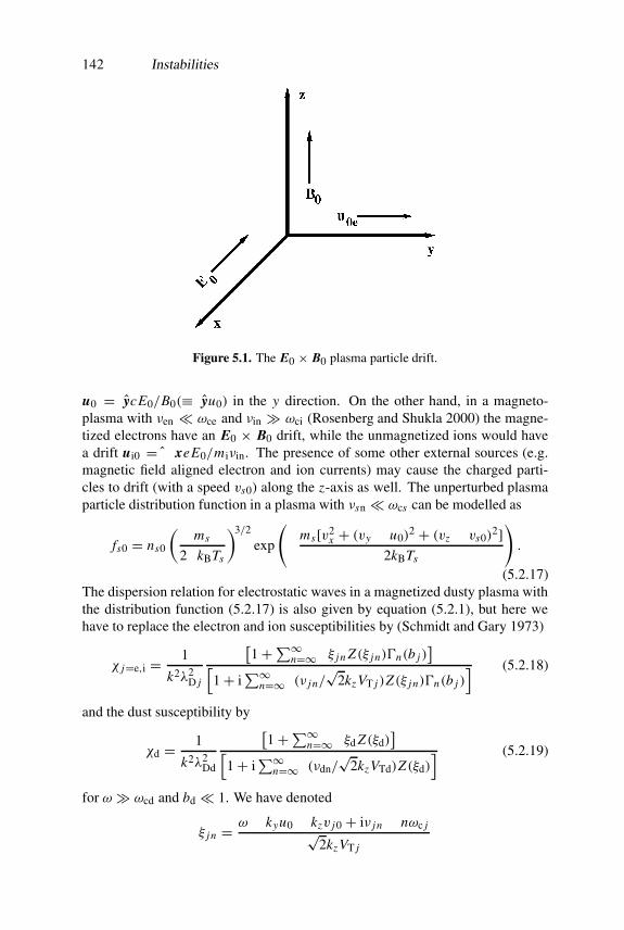
142 Instabilities
Figure 5.1. The E0 × B0 plasma particle drift.
u0 = ycE0/B0(≡ yu0) in the y direction. On the other hand, in a magneto-plasma with νen � ωce and νin � ωci (Rosenberg and Shukla 2000) the magne-tized electrons have an E0 × B0 drift, while the unmagnetized ions would havea drift ui0 = −xeE0/miνin. The presence of some other external sources (e.g.magnetic field aligned electron and ion currents) may cause the charged parti-cles to drift (with a speed vs0) along the z-axis as well. The unperturbed plasmaparticle distribution function in a plasma with νsn � ωcs can be modelled as
fs0 = ns0
(ms
2πkBTs
)3/2
exp
(−ms[v2
x + (vy − u0)2 + (vz − vs0)
2]2kBTs
).
(5.2.17)The dispersion relation for electrostatic waves in a magnetized dusty plasma withthe distribution function (5.2.17) is also given by equation (5.2.1), but here wehave to replace the electron and ion susceptibilities by (Schmidt and Gary 1973)
χ j=e,i = 1
k2λ2D j
[1+∑∞
n=−∞ ξ j n Z(ξ j n)�n(b j )]
[1+ i
∑∞n=−∞(ν j n/
√2kz VT j )Z(ξ j n)�n(b j )
] (5.2.18)
and the dust susceptibility by
χd = 1
k2λ2Dd
[1+∑∞
n=−∞ ξd Z(ξd)]
[1+ i
∑∞n=−∞(νdn/
√2kzVTd)Z(ξd)
] (5.2.19)
for ω � ωcd and bd � 1. We have denoted
ξ j n = ω − kyu0 − kzv j0 + iν j n − nωc j√2kzVT j

Streaming Instabilities 143
and
ξd = ω − kyu0 − kzvd0 + iνdn√2kVTd
.
We now consider a collisionless dusty magnetoplasma without the dc electric fieldand focus on both hydrodynamic and kinetic instabilities.
5.2.2.1 Hydrodynamic instability
We first consider the ion–dust two-stream instability of long-wavelength (namelybs � 1) modes. Assuming ξe � 1, ξi,d � 1, ωcd, kVTd, kzvd0 � ω � νen �kzVTe, and νin, kzVTi � |ω − kzvi0| � ωci, we can reduce equations (5.2.1),(5.2.18) and (5.2.19) to the form
1− ω2pik
2z
Ab(ω − kzvi0)2k2− ω2
pd
Abω2= 0 (5.2.20)
where Ab = 1+ (kλDe)−2+ω2
pik2⊥/ω2
cik2. For kzvi0 � ω equation (5.2.20) gives
ωr � ωi �(ωpikz
ωpdk
)1/3 ωpd
A1/2b
(5.2.21)
with the maximum growth rate at kzvi0 � ωpikz/k A1/2b .
5.2.2.2 Kinetic instability
To study kinetic instability in a dusty magnetoplasma, we consider two typesof electrostatic modes, namely electrostatic ion-cyclotron (EIC) waves andelectrostatic dust cyclotron (EDC) waves.
(i) EIC waves
We consider kinetic instability of EIC waves (ω ∼ ωci) in a collisionless dustyplasma in the presence of an equilibrium electron flow along z. For ξe � 1, be �1, |ω−kzve0| � kzVTe, |ω−nωci| � kzVTi, and νdn, kVTd � ω � νen � kzVTe,the various dielectric susceptibilities are of the form (Chow and Rosenberg 1995)
χe ≈ 1+ 1
k2λ2De
[1+ i
√π
2
(ω − kzve0)
kzVTe
](5.2.22)
χi ≈ 1
k2λ2Di
{1− �1(bi)
ω
ω − ωci− 1− �0(bi)
bi
+ i
√π
2
ω
kz VTi�0(bi) exp
[−(ω − ωci√
2kz VTi
)2]}(5.2.23)

144 Instabilities
and χd ≈ −ω2pd/ω
2. When ω � ωci � ωpd, the dust contribution to thedispersion relation is small, namely χd � χi. The dust influences the instabilityonly via the quasi-neutrality condition, but not through its dynamics. Hence usingequations (5.2.1), (5.2.22) and (5.2.23) and letting ω = ωr + iωi, we obtain
ωr ≈ ωci(1+ δs)1/2 (5.2.24)
and the growth rate (Chow and Rosenberg 1995)
ωi ≈√π
8
(ωr − ωci)2
�1(bi)ωci
{ne0Ti
ni0Te
kzve0 − ωr
kzVTe
− �1(bi)ωr
kzVTiexp
[−(ωr − ωci√
2kzVTi
)2]}(5.2.25)
where we have denoted
δs = �1(bi)
1− �1(bi)− b−1i [1− �0(bi)] + ne0Ti(1+ k2λ2
De)/ni0Te.
Equation (5.2.25) admits an oscillatory instability of the EIC waves when kzve0 >
ωr � ωi. For bi � 1 and k2λ2De � 1 we have δs ≈ k2⊥C2
S/ω2ci and
ωr ≈ ωci(1+ k2⊥C2S/ω
2ci)
1/2. The corresponding growth rate is
ωi ≈√π
8
1
k2⊥λ2De
|kzve0 − ωr|kzVTe
(ω2r − ω2
ci)2
ωrω2pi
(5.2.26)
which far exceeds the ion cyclotron damping rate, given by the second term in thecurly bracket in the right-hand side of equation (5.2.25).
(ii) EDC waves
The kinetic instability of EDC waves (D’Angelo 1990) with ξe � 1, ω � νen �kzVTe, νin � kVTi, |ω − ωcd| � kVTd and ρTe � k−1
⊥ � ρTi in the presence ofthe streaming ions can be investigated by means of the dispersion relation
1+ 1
k2λ2D
+ 1
k2λ2Dd
[1− �0(bd)− 2ω2�1(bd)
(ω2 − ω2cd)
]+ i
√π
2
1
k2λ2Di
ω − kzvi0
kVTi= 0.
(5.2.27)Letting ω = ωr + iωi into equation (5.2.27), where ωi � ωr, we obtain
ωr = ωcd
(1−()1/2 (5.2.28)
and the growth rate
ωi ≈√
π
32
|kzvi0 − ωr|kVTi
λ2Dd
λ2Di
(ω2r − ω2
cd)2
ω2cdωr�1(bd)
(5.2.29)
Streaming Instabilities 145
where
( = 1− λ2D
λ2Dd
2�1(bd)
(1+ k2λ2D + λ2
D[1− �0(bd)]/λ2Dd)
. (5.2.30)
Equation (5.2.29) exhibits that the EDC waves would grow if kzvi0 > ωr. Forbd � 1 and k2λ2
D � 1 the growth rate is
ωi ≈√π
8
1
k2⊥λ2Di
|kzvi0 − ωr|kVTi
(ω2r − ω2
cd)2
ω2pdωr
(5.2.31)
with ωr = ωcd(1+ k2⊥C2D/ω
2cd)
1/2.
5.2.3 Boundary effects
We have discussed instabilities of numerous electrostatic waves in an infiniteplasma. However, for laboratory dusty plasmas those instabilities have to bereconsidered in a longitudinally bounded dusty plasma system. Accordingly, wediscuss an example of the ion beam instability in a collisionless unmagnetizedbounded dusty plasma (Rosenberg and Shukla 1998). We assume that thestreaming ions, which comprise an ion beam, flow from a grounded grid at z = 0in the dusty plasma to a target at z = L. The grid and the target have infiniteextent in the x and y directions. In the steady state, the zeroth-order drifts in thez direction are Vi0 ≡ U0 � VTi and Ve0 = Vd0 = 0.
The one-dimensional DIA wave behaviour is governed by the continuity andmomentum equations for the ion and dust fluids, supplemented by a Boltzmanndistribution (equation (4.2.1)) for the electrons and Poisson’s equation for thewave potential φ. From the linearized equations for the DIA waves, we easilyobtain the dispersion relation by assuming that the density perturbations and thewave potential vary as exp(−iωt + ikz). The result for an unbounded plasma is
k2
[1+ k2
De
k2− ω2
pi
(ω − kU0)2− ω2
pd
ω2
]= 0. (5.2.32)
We consider the effect of longitudinal boundaries on the instability analysis(Iizuka et al 1985). Two roots of equation (5.2.32) for ω � kU0 are
k1,2 ≈ ±ωpi
U0
1− U 2
0C2
S
1− ω2pd
ω2
1/21±
(1− ω2
pd
ω2
)1/2
(1− U 3
0
C3S
) ω
ωpi
. (5.2.33)
It is straightforward to obtain a dispersion relation for a bounded dusty plasma inthe frequency domain ωpi � ω � (ω2
pdωpi)1/3 > ωpd. The procedure (Iizuka et
al 1985) involves using the other two roots of equation (5.2.32), which come from

146 Instabilities
the spatial derivative ∂2φ/∂z2, expressing the perturbations in the system usingthese four roots and using the following boundary conditions on the potentialperturbation and the perturbed ion density and velocity: φ(z = 0) = φ(z = L) =0 (the potential perturbations are assumed to be zero at the end electrodes) andni1(z = 0) = vi(z = 0) = 0 (since the unperturbed ion beam is injected at thegrid). This yields (Rosenberg and Shukla 1998)
sinϑ + ω2pd
2ω2ϑ cosϑ + iω
ωpi
X
ϑ
[X2 sinϑ
ϑ+ 2(cosϑ − 1)
]= 0 (5.2.34)
where ϑ2 = X2 − D2, X = ωpiL/U0 and D = kDeL. We note that ϑ2 > 0requires ni0Te/ne0Ti > U2
0 /V 2Ti in the dusty plasma.
We consider the solutions of equation (5.2.34) in two regimes; onecorresponding to an ion–dust Buneman-type instability driven by the ion beamin which case the dust dynamics are retained, and the other corresponding to thePierce instability of the ion beam. Now retaining the dust dynamics, we find thatequation (5.2.34) admits a strongly unstable solution when ϑ ≈ π(2m−1), wherem = 1, 2, 3, . . . . At ϑ = (2m − 1)π = Sπ equation (5.2.34) gives (Rosenbergand Shukla 1998)
ω2pd
ω2+ i
ω
ωpi
8
Sπ
(1+ k2
DeL2
S2π2
)1/2 ≈ 0. (5.2.35)
An unstable root of equation (5.2.35) is
ω
ωpd= (
√3+ i)
2
(1+ k2
De L2
S2π2
)1/6
(Sπ
8
)1/3 ( ωpi
ωpd
)1/3
. (5.2.36)
We can also define a characteristic current associated with this ion–dust Bunemaninstability when ϑ = Sπ . Since from the latter condition we have ω2
pi =k2
DeU20 + S2π2/L2, the ion beam current Ii = eni0U0πR2
b is given by
Ii ∼ R2b
mi
4e
S2π2
L2U3
0
(1+ k2
DeL2
S2π2
)(5.2.37)
where Rb is the beam radius. We note that for m = 1 at ϑ = π , the ion beamcurrent is smaller than the characteristic current for the usual Buneman instabilityof the electron beam in a bounded electron beam plasma system. This is due toVTe � U0 � VTi for the ion beam case, whereas for the electron beam case wehave U0 � VTe.
An aperiodic instability of the ion beam can be obtained fromequation (5.2.34) by neglecting the dust dynamics, i.e. in the limit md → ∞.

Ion Drag Force Induced Instabilities 147
This gives a purely imaginary solution
ω
ωpi≈ i
ϑ2
X
sinϑ
[X2 sinϑ + 2ϑ(cosϑ − 1)] (5.2.38)
which corresponds to a Pierce instability of the ion beam including screening bythe electrons. Thus, for large L and ϑ �= Sπ , we obtain
ω � iU0
L
(1− U2
0
C2S
). (5.2.39)
Let us now consider a possible application of the present results for designinga dusty plasma diode system to study the physics of bounded beam–plasmasystems. To investigate longitudinal boundary effects on the ion–dust Bunemaninstability, the system should have ϑ ∼ π(2m − 1), where m is low. Since
ϑ2 =(
C2S
U20
− 1
)k2
DeL2 ≡(
ni0Te
ne0Ti
V 2Ti
U20
− 1
)L2
λ2De
(5.2.40)
one would require that the first term in parentheses in equation (5.2.40) is muchsmaller than 1 when L � λDe. For example, using ne0 � 108 cm−3 andkBTe � 3 eV we obtain λDe � 0.1 cm. Then, if ni0/ne0 � 1.01, U0/VTi � 3 andTe/Ti � 9, the m = 2 mode might be observed if L � 9 cm. We also note thatin this case the growth rate of the Pierce instability, as given by equation (5.2.39),would be significantly reduced. However, the ion–dust Buneman instabilitypersists in the large-L regime where the effects of longitudinal boundaries can beneglected. Thus, the interplay between that instability and the Pierce instability ofthe ion beam might be investigated in that regime. As an example, let us considera N2 plasma with ni0 � 4 × 108 cm−3, nd0/ni0 � 4 × 10⁻⁴, md/mi � 1010
(corresponding to dust with a radius rd � 0.5 µm) and Zd � 1.3×10³ (assumingkBTe � 2 eV). The growth rate of the ion–dust Buneman instability for theseparameters is (ωpiω
2pd)
1/3 � 16 × 103 s−1. If the ions stream with a speed
U0 � 2 × 105 cm s−1 (corresponding to U0/VTi � 3 for kBTi � 0.1 eV), thegrowth rate (�U0/L) of the Pierce instability of the ion beam would be of thesame order as the growth rate of the ion–dust Buneman instability for L � 25 cm.
5.3 Ion Drag Force Induced Instabilities
Radio-frequency capacitively coupled argon and silane discharges are oftenemployed for generating dust particles (Prabhuram and Goree 1996, Melzer etal 1998, Samsonov and Goree 1999). The dust particles in these dischargesgrow from molecule size to a few hundred nanometres in diameter. The particlesusually fill the entire plasma volume, although dust-free regions, or so-called ‘dustvoids’, have been observed in silane and other dust-laden plasmas. Furthermore,

148 Instabilities
in a partially ionized dusty plasma, ionization of neutral atoms plays a crucialrole. Accordingly, studies of instabilities in the presence of the ion drag force andionization is of practical interest in processing plasmas.
As mentioned in chapter 3, the ion drag force arises from the ion orbitalmotion around negatively charged dust particles as well as from the momentumtransfer from all the ions which are collected by the dust grains. The instabilitymay arise due to the ion fluid compression by the ion drag force. The latter,which is proportional to the square of the particle radius, dominates over theelectrostatic force when the dust grains have sufficiently large sizes. Here weconsider instabilities of electrostatic waves whose frequency is much smaller thanνen and whose wavelength is much shorter than VTe/νen. The electron numberdensity in such a situation is given by equation (4.2.1). The dynamics of the ionsand negatively charged dust grains in the presence of ionization and ion drag forceis governed by a set of equations (D’Angelo 1997, 1998, Shukla and Morfill 1999)comprising the ion continuity equation
∂ni
∂ t+ ∇ · (nivi) = −QL + Qi (5.3.1)
the ion momentum equation
mi
(∂
∂ t+ vi · ∇ + νin + Qi
ni− µi∇2
)vi = −e∇φ − γikBTi
ni0∇ni (5.3.2)
the dust continuity equation (4.2.3), the dust momentum equation
md
(∂
∂ t+ vd · ∇ + νdn
)vd = Zd0e∇φ + md g + Fdi (5.3.3)
and the quasi-neutrality condition ni = ne + Zd0nd. Here QL = νlni, νl is theion loss rate occurring both to the walls of the plasma container and to the dustgrains within the plasma, Qi (= σi0nnψi, where σi0 is the ionization cross sectionand ψi is the flux of ionizing electrons) accounts for the creation of new ionsthrough ionization of the neutral atoms by fast electrons and µi is the coefficientof the kinematic ion viscosity. For simplicity, dust charge fluctuations have beenignored and the neutrals are assumed to be immobile.
We assume that the ion drag force Fdi arising form the ion orbital motionaround the dust grains dominates over that arising from the momentum transferfrom all the ions that are collected by the dust grains. This is justified as long asthe collection impact parameter is much smaller than the orbital impact parameterand the Coulomb logarithm far exceeds 1. Thus, the orbital motion related iondrag force acting on the dust grains takes the form
Fdi = nimiVitvi4πb2π/2'(Vit) (5.3.4)
where Vit = (v2i + 8V 2
Ti/π)1/2, b2
π/2 = Z2d0e4/m2
i V 4it is the orbital impact
parameter and'(Vit) = ln[(λ2De+b2
π/2)/(b2c+b2
π/2)]1/2 is the Coulomb logarithm

Ion Drag Force Induced Instabilities 149
integrated over the interval from the collection impact parameter bc = rd(1 +2Zd0e2/rdmiV 2
it ) to the electron Debye radius λDe. Clearly, the ion drag forcedepends on the ion velocity as well as on the dust grain charge. In the absence ofequilibrium dust streaming and the dc electric field, the dust grains are held underthe combined influence of the gravity force and the equilibrium ion drag forceinvolving unperturbed ion flow towards the dust grain surface.
We now study the instability of an equilibrium dusty plasma againstelectrostatic waves. Thus, the densities, fluid velocities as well as the ionizationand the ion drag force are perturbed. Accordingly, we let ns = ns0 + ns1and σi0 = σ0 + (dσi0/dφ)0φ, where ns1 � ns0 and σ0 represents some valueof the ionization cross section slightly above the threshold, when the ion flowand unperturbed dust plasma densities are uniform. In zeroth order, we haveνlni0 = σ0nn0ψi. Now substituting the perturbed electron number density (e.g.equation (4.2.1)) into the perturbed quasi-neutrality condition, we have
ni1 = ne0eφ
kBTe+ Zd0nd1. (5.3.5)
The linearized equations (5.3.1) and (5.3.2) are written as, respectively(∂
∂ t+ vi0 ·∇ + νl
)ni1 + ni0∇ · vi = Adφ (5.3.6)
and(∂
∂ t+ vi0 ·∇ + νin + Qi0
ni0− µi∇2
)vi = − e
mi∇(φ + γikBTi
e
ni1
ni0
)(5.3.7)
where vi0 is the unperturbed ion streaming velocity, Ad = (dσi0/dφ)0nn0ψi andQi0 = σ0nn0ψi ≡ νlni0. On the other hand, from equations (4.2.3) and (5.3.3)one obtains(
∂
∂ t+ νdn
)∂nd1
∂ t= −nd0 Zd0e
md∇2φ − 8
√2πnd0ni0miVTib2
id'0
md∇ · vi (5.3.8)
where b2id ≈ π2 Z2
d0e4/64k2BT 2
i (1 + pi)3/2, pi = πv2
i0/8V 2Ti, '0 = '(Vit0) and
Vit0 = (v2i0+ 8V 2
Ti/π)1/2. We now derive the dispersion relations for the DIA and
DA waves in a collisional dusty plasma by using equations (5.3.5)–(5.3.8).
5.3.1 DIA waves
To study the DIA waves, we assume |(∂/∂ t)+ vi0 ·∇ − µi∇2| � νin + νl ≡ νil .Thus, equation (5.3.7) gives
vi ≈ − e
miνil∇(φ + γikBTi
e
ni1
ni0
). (5.3.9)
150 Instabilities
Now substituting vi from equation (5.3.9) into equation (5.3.6), we have(∂
∂ t+ vi0 · ∇ + νl − Di∇2
)ni1 = ni0
(e
miνil∇2 + Ad
ni0
)φ (5.3.10)
where Di = γiV 2Ti/νil . Eliminating vi from equations (5.3.8) and (5.3.9) we obtain(
∂
∂ t+ νdn
)∂nd1
∂ t= −nd0 Zd0e
md∇2φ + nd0eαi
md∇2(φ + γikBTi
e
ni1
ni0
)(5.3.11)
where αi = √π/2Z2
d0'0ωpi/64νil�(1 + pi)3/2 and � = ni0λ
3Di.
Equations (5.3.5), (5.3.10) and (5.3.11) are the desired equations for studying theinstability of low-frequency DIA waves in a collisional dusty plasma includingionization and the orbital ion drag force.
Let us now Fourier transform equations (5.3.10) and (5.3.11), combine theresultant expressions and use equation (5.3.5) to obtain the dispersion relation forthe DIA waves (Shukla and Morfill 1999)
[ω(ω + iνdn)− k2C2i ](ω − k · vi0 + i�i + iνl + i�s − iωI)
= k2C2De(ω − k · vi0 + i�i + iνl )
(1− αiτi
Zd0
)(5.3.12)
where C2i = Zd0nd0γikBTiαi/ni0md, �i = Dik2, �s = k2C2
S/νil , ωI =νl Iσ , Iσ = (ne0kBTe/ni0eσ0)(dσi0/dφ)0, CDe = ωpdλDe and τi = 1 +ne0γiTi/ni0Te. Two comments are in order.
(i) When the electrostatic and ion drag forces exactly balance each other, i.e.when Zd0 = αiτi, equation (5.3.12) yields ω = −i(νdn/2) ± (k2C2
i −ν2
dn/4)1/2 and ω = k · vi0 − i(�i + νl + �s) + iωI. The latter predictsan ionization instability if ωI > �i + νl +�s .
(ii) When we assume |ω − k · vi0 + iνl + i�i| � �s, ωI and |ω| � νdn, kCi,equation (5.3.12) gives a purely growing (ω = iωi) instability provided thatαiτi > Zd0. The latter indicates that the origin of the instability is theion orbital drag force which causes the ion fluid compression that is out ofphase with the dust fluid perturbation. Thus, energy stored in the ion flow iscoupled to low-frequency density perturbations which temporally grow. Wenote that the ion drag force driven instability occurs when
Zd0 >64νil�(1+ pi)
3/2
ωpi'0τi. (5.3.13)
Since Zd0 is proportional to the dust radius, the latter is a decisive parameterfor the onset of the instability due to the ion drag force. The interplaybetween ionization and the ion drag drivers can be studied by numericallyanalysing equation (5.3.12).
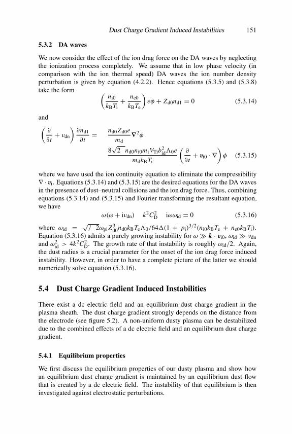
Dust Charge Gradient Induced Instabilities 151
5.3.2 DA waves
We now consider the effect of the ion drag force on the DA waves by neglectingthe ionization process completely. We assume that in low phase velocity (incomparison with the ion thermal speed) DA waves the ion number densityperturbation is given by equation (4.2.2). Hence equations (5.3.5) and (5.3.8)take the form (
ni0
kBTi+ ne0
kBTe
)eφ + Zd0nd1 = 0 (5.3.14)
and(∂
∂ t+ νdn
)∂nd1
∂ t= − nd0 Zd0e
md∇2φ
− 8√
2πnd0ni0miVTib2id'0e
mdkBTi
(∂
∂ t+ vi0 · ∇
)φ (5.3.15)
where we have used the ion continuity equation to eliminate the compressibility∇ · vi. Equations (5.3.14) and (5.3.15) are the desired equations for the DA wavesin the presence of dust–neutral collisions and the ion drag force. Thus, combiningequations (5.3.14) and (5.3.15) and Fourier transforming the resultant equation,we have
ω(ω + iνdn)− k2C2D − iωωid = 0 (5.3.16)
where ωid = √π/2ωpi Z3
d0nd0kBTe'0/64�(1 + pi)3/2(ni0kBTe + ne0kBTi).
Equation (5.3.16) admits a purely growing instability for ω � k · vi0, ωid � νdnand ω2
id > 4k2C2D. The growth rate of that instability is roughly ωid/2. Again,
the dust radius is a crucial parameter for the onset of the ion drag force inducedinstability. However, in order to have a complete picture of the latter we shouldnumerically solve equation (5.3.16).
5.4 Dust Charge Gradient Induced Instabilities
There exist a dc electric field and an equilibrium dust charge gradient in theplasma sheath. The dust charge gradient strongly depends on the distance fromthe electrode (see figure 5.2). A non-uniform dusty plasma can be destabilizeddue to the combined effects of a dc electric field and an equilibrium dust chargegradient.
5.4.1 Equilibrium properties
We first discuss the equilibrium properties of our dusty plasma and show howan equilibrium dust charge gradient is maintained by an equilibrium dust flowthat is created by a dc electric field. The instability of that equilibrium is theninvestigated against electrostatic perturbations.
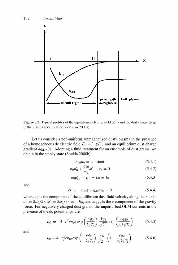
152 Instabilities
Figure 5.2. Typical profiles of the equilibrium electric field (E0) and the dust charge (qd0)in the plasma sheath (after Ivlev et al 2000a).
Let us consider a non-uniform, unmagnetized dusty plasma in the presenceof a homogeneous dc electric field E0 = − zE0z and an equilibrium dust chargegradient ∂qd0/∂z. Adopting a fluid treatment for an ensemble of dust grains, weobtain in the steady state (Shukla 2000b)
nd0u0 = constant (5.4.1)
u0u′0 +qd0
mdφ′0 + gz = 0 (5.4.2)
u0q ′d0 = Ie0 + Ii0 ≡ I0 (5.4.3)
ande(ni0 − ne0)+ qd0nd0 = 0 (5.4.4)
where u0 is the component of the equilibrium dust fluid velocity along the z-axis,u′0 = ∂u0/∂z, φ′0 = ∂φ0/∂z ≡ −E0z and mdgz is the z component of the gravityforce. For negatively charged dust grains, the unperturbed OLM currents in thepresence of the dc potential φ0 are
Ie0 = −4πr2d ene0 exp
(eφ0
kBTe
)VTe√
2πexp
(eqd0
rdkBTe
)(5.4.5)
and
Ii0 = 4πr2d eni0 exp
(− eφ0
kBTi
)VTi√2π
(1− eqd0
rdkBTi
). (5.4.6)

Dust Charge Gradient Induced Instabilities 153
Equations (5.4.1)–(5.4.4) reveal that in the absence of the equilibrium dust fluidvelocity, we have qd0 E0z = mdgz and Ie0 + Ii0 = 0. The latter determinesthe equilibrium charge on the dust grain surface, while the former dictates thata balance between the sheath electric and gravity forces is responsible for thelevitation of the dust grains. On the other hand, in the presence of a uniform dustflow there appears a dust charge gradient q ′d0 = I0/u0, which can be expressed as
q ′d0 = −4πr2d eα0
[Ne exp
(eqd0
rdkBTe
)− Ni
VTi
VTe
(1− eqd0
rdkBTi
)](5.4.7)
where Ne = ne0 exp(eφ0/kBTe), Ni = ni0 exp(−eφ0/kBTi) and α0 =VTe/
√2πu0.
5.4.2 DA waves
To study the instability of our equilibrium state against the DA waves, we letnd = nd0 + nd1, vd = u0 z + u1, φ = φ0(z) + φ1 and qd = qd0(z) + q1,where nd0 and u0 are uniform and n1, u1, φ1 and q1 are small perturbationsof their equilibrium values. Hence we obtain from the dust continuity and dustmomentum equations (Shukla 2000b)
dnd1
dt+ nd0∇ · u1 = 0 (5.4.8)
anddu1
dt+ qd0
md∇φ1 + φ′0
mdq1 = 0. (5.4.9)
The Poisson equation takes the form
∇2φ1 = k2Dφ1 − 4π(qd0nd1 + nd0q1) (5.4.10)
while the dust grain charging equation reads
dq1
dt+ ν1q1 + q ′d0u1z = −ν2rdφ1 (5.4.11)
where d/dt = (∂/∂ t)+u0(∂/∂z). Note that equations (5.4.9) and (5.4.11) containthe terms φ′0q1/md and q ′d0u1z , which are associated with perturbed electrostaticforces involving the unperturbed sheath electric field and the advection of theequilibrium dust charge gradient by the dust fluid velocity u1z , respectively. Thesetwo forces are responsible for the novel absolute instabilities, as described below.
The dispersion relation can be obtained by combining (5.4.8)–(5.4.11) andFourier transforming the resultant equation by supposing that the perturbedquantities are proportional to exp(−iωt + iky). Accordingly, for k2/k2
D � 1we obtain (Shukla 2000b)
1− ω2D
ω2 +(
1+ �2D
ω2
)k2
qλ2Dν1
ν1 − i(ω +�)= 0 (5.4.12)
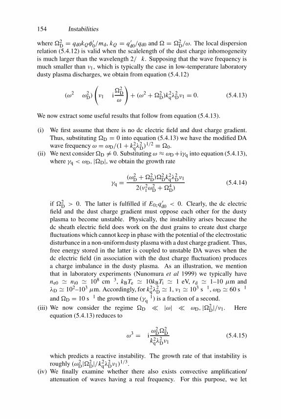
154 Instabilities
where �2D = qd0kQφ
′0/md, kQ = q ′d0/qd0 and � = �2
D/ω. The local dispersionrelation (5.4.12) is valid when the scalelength of the dust charge inhomogeneityis much larger than the wavelength 2π/k. Supposing that the wave frequency ismuch smaller than ν1, which is typically the case in low-temperature laboratorydusty plasma discharges, we obtain from equation (5.4.12)
(ω2 − ω2D)
(ν1 − i
�2D
ω
)+ (ω2 +�2
D)k2qλ
2Dν1 = 0. (5.4.13)
We now extract some useful results that follow from equation (5.4.13).
(i) We first assume that there is no dc electric field and dust charge gradient.Thus, substituting �D = 0 into equation (5.4.13) we have the modified DAwave frequency ω = ωD/(1+ k2
qλ2D)
1/2 ≡ �0.(ii) We next consider�D �= 0. Substituting ω ≈ ωD+ iγq into equation (5.4.13),
where γq < ωD, |�D|, we obtain the growth rate
γq =(ω2
D +�2D)�
2Dk2
qλ2Dν1
2(ν21ω
2D +�4
D)(5.4.14)
if �2D > 0. The latter is fulfilled if E0zq ′d0 < 0. Clearly, the dc electric
field and the dust charge gradient must oppose each other for the dustyplasma to become unstable. Physically, the instability arises because thedc sheath electric field does work on the dust grains to create dust chargefluctuations which cannot keep in phase with the potential of the electrostaticdisturbance in a non-uniform dusty plasma with a dust charge gradient. Thus,free energy stored in the latter is coupled to unstable DA waves when thedc electric field (in association with the dust charge fluctuation) producesa charge imbalance in the dusty plasma. As an illustration, we mentionthat in laboratory experiments (Nunomura et al 1999) we typically havene0 � ni0 � 108 cm−3, kBTe � 10kBTi � 1 eV, rd � 1–10 µm andλD � 102–103 µm. Accordingly, for k2
qλ2D � 1, ν1 � 103 s−1, ωD � 60 s−1
and �D = 10 s−1 the growth time (γ−1q ) is a fraction of a second.
(iii) We now consider the regime �D � |ω| � ωD, |�2D|/ν1. Here
equation (5.4.13) reduces to
ω3 = −iω2
D�2D
k2qλ
2Dν1
(5.4.15)
which predicts a reactive instability. The growth rate of that instability isroughly (ω2
D|�2D|/k2
qλ2Dν1)
1/3.(iv) We finally examine whether there also exists convective amplification/
attenuation of waves having a real frequency. For this purpose, we let

Dust Charge Gradient Induced Instabilities 155
k = kr + iki in equation (5.4.12) and obtain the real (kr) and imaginary(ki) parts of the wavenumber. We have
k2r = k2
i +ω2
C2D
[1+ (ω2 +�2
D)ν21 k2
qλ2D
ν21ω
2 + (ω2 +�2D)
2
](5.4.16)
and
ki = ων1
krC2D
(ω2 +�2D)
2
ω2pd
k2qλ
2D
ν21ω
2 + (ω2 +�2D)
2. (5.4.17)
It turns out that equation (5.4.17) does not admit a convective instability, butone encounters only a spatial attenuation of the waves.
5.4.3 Transverse DL waves
We now discuss the dispersion properties of the transverse DL (TDL) waves onthe one-dimensional dust particle chain in a strongly coupled Yukawa (or theDebye–Huckel) system by incorporating the dust charge gradient effect. Weconsider the vibration of the one-dimensional horizontal chain of dust particlesof equal mass md separated by the distance a. When the nth dust particle isvertically displaced from its equilibrium position, it experiences forces due tointergrain interactions through a Debye-screened Coulomb force and through adirect interaction with a vertically varying sheath electric field E0. The balanceof these forces in the linear approximation with respect to a small verticaldisplacement δzn of the nth particle at the equilibrium zn = z0 gives the equationof motion for vertical oscillations (Miswa et al 2001)
∂2δzn
∂ t2+ νdn
∂δzn
∂ t= −ω2
γ δzn +�2t (2δzn − δzn−1 − δzn+1)+ E0δqn
md(5.4.18)
where ω2γ = γr/md, γr is the restoring force coefficient for a single particle
oscillating in an electrostatic potential well
�2t =
q2d0
mda3
(1+ a
λD
)exp
(− a
λD
)(5.4.19)
is the quantity related to the screened interparticle potential, qd0 is the equilibriumcharge of the dust particle levitated at the equilibrium position z0 and δqn is thecharge deviation from qd0 associated with the inhomogeneous qd0 variation in thevertical direction and the delayed charging due to the finite charging time whenthe dust particle oscillates through the sheath. The last term in the right-hand sideof equation (5.4.18) represents the perturbed electric force acting on a dust particledue to the charge variation. The force becomes positive or negative depending onthe signs of δqn and E0 around the equilibrium, which may lead to damping (or

156 Instabilities
growth) of the TDL waves. The time variation of δqn is modelled by the equation(Ivlev et al 2000a, Miswa et al 2001)
∂δqn
δt= −νcδqn + νc
(∂qd0
∂z
)z=z0
δzn (5.4.20)
where νc is the typical charging frequency for the dust particle. Equation (5.4.20)shows that when the charging time τc is sufficiently large, we have δqn =(∂qd0/∂z)z=z0δzn , which indicates that the charge takes a value determined by theinstantaneous vertical position. On the other hand, if νc tends to zero, δqn tendsto zero and the charge retains its original value. For a typical TDL wave withfinite νc/ω � 1, one may assume that δzn and δqn oscillate as exp(−iωt + ikna).Hence from equations (5.4.18) and (5.4.20) we obtain the modified TDL wavedispersion relation (Miswa et al 2001)
ω2 + iν∗ω = ω2γ ∗ −�2
t [2− exp(ika)− exp(−ika)] (5.4.21)
where ν∗ = νdn − �∗, �∗ = −(E0/mdνc)(∂qd0/∂z)z=z0 , ω2γ ∗ = γ∗/md and
γ∗ = γr−E0(∂qd0/∂z)z=z0 . It is evident from equation (5.4.21) that the imaginarypart of k arises from not only due to the neutral drag force, but also from thedelayed charging effect �∗. The latter has little effect on the real part of k.However, the imaginary part of k is found to be influenced by the delayed chargingeffect. Miswa et al (2001) found that if �∗ takes a large positive value to yield thecondition ν∗ < 0, one may have instability of the TDL waves. Furthermore, inthe absence of the dust charge gradient and the dc electric field, equation (5.4.21)takes the form
ω2 + iνdnω = ω2γ − 4�2
t sin2(
ka
2
)(5.4.22)
which yields ω = ±ωγ for k = 0.
5.5 Drift Wave Instabilities
It is well known that free energy stored in equilibrium density, temperature andvelocity gradients can be coupled to electrostatic and electromagnetic waves in amagnetized electron–ion plasma (Ichimaru 1973, Weiland 2000). Here we discussinstabilities of electrostatic waves in a non-uniform dusty plasma in a uniformmagnetic field zB0.
5.5.1 Universal instability
The presence of an equilibrium dust charge gradient (∂qd0/∂x) can produceinstability of low-frequency (�ωci) electrostatic drift waves in a non-uniformmagnetized plasma which also contains a density gradient ∂ne0/∂x along thex-axis. Since the drift wave frequency is typically much larger than the dust

Drift Wave Instabilities 157
plasma and dust gyro-frequencies, the dust grains can be considered immobile.The electron number density perturbation in this case is (Ichimaru 1973, Weiland2000)
ne1 = k2
4πeχeφ ≡ ne0
(1+ i
√π
2
ω + ωe∗kzVTe
)eφ
kBTe(5.5.1)
where the electron susceptibility χe has been deduced from the generalsusceptibility (Miyamoto 1980, Stenflo 1981)
χ j ≈ 1
k2λ2D j
{1−
∞∑n=−∞
�n(b j )
[ω + ω j∗
(1+ nω
b jωc j
)]% j
}(5.5.2)
in the limits be � 1, ω � ωce and |ω + ω j∗| � kzVTe. Here wehave denoted ω j∗ = (kyckBTj/eB0n j0)(∂n j0/∂x) ≡ kyckBTe/eB0L j , % j =∫∞∞ Fz dvz/(ω − kzvz − nωc j ) and Fz = (2πV 2
T j )−1/2 exp(−v2
z /2V 2T j ). The ion
density perturbation is given by
ni1 = − k2
4πeχiφ ≡ −ni0
(Te
Ti
ωi∗ω+ k2⊥c2
s
ω2ci
)eφ
kBTe(5.5.3)
where the ion susceptibility has been obtained from equation (5.5.2) by assumingbi � 1 and kz VTi � ω � ωci. By invoking the quasi-neutrality condition,namely ne1 = ni1, we then obtain from equations (5.5.1) and (5.5.3)
1+ i
√π
2
ω + ωe∗kz VTe
+ ni0Te
ne0Ti
ωi∗ω+ k2⊥ρ2
s = 0 (5.5.4)
which is the dispersion relation for the drift waves in a dusty plasma. Lettingω = ωr + iωi in equation (5.5.4) and assuming k2⊥ρ2
s � 1 we obtain the real partof the dust drift wave frequency (Shukla et al 1991)
ωr = −ni0Te
ne0Tiωi∗ (5.5.5)
and the growth/damping rate (Benkadda et al 1995)
ωi =√π
2ωr
kyckBTe
e2 B0ne0kz VTe
∂(nd0qd0)
∂x(5.5.6)
where we have used the relation
ωe∗ − ni0Te
ne0Tiωi∗ = kyckBTe
e2 B0ne0
∂(nd0qd0)
∂x. (5.5.7)
Equation (5.5.6) reveals that long-wavelength (in comparison with ρs) drift wavesare universally unstable in a dusty plasma with ∂(nd0qd0)/∂x > 0. The instabilityis caused by the wave–electron interaction in a magnetoplasma containing eitherdensity or charge gradient.
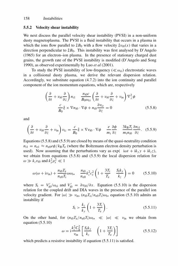
158 Instabilities
5.5.2 Velocity shear instability
We next discuss the parallel velocity shear instability (PVSI) in a non-uniformdusty magnetoplasma. The PVSI is a fluid instability that occurs in a plasma inwhich the ions flow parallel to zB0 with a flow velocity zvi0(x) that varies in adirection perpendicular to zB0. This instability was first analysed by D’Angelo(1965) for an electron–ion plasma. In the presence of stationary charged dustgrains, the growth rate of the PVSI instability is modified (D’Angelo and Song1990), as observed experimentally by Luo et al (2001).
To study the PVSI instability of low-frequency (�ωci) electrostatic wavesin a collisional dusty plasma, we derive the relevant dispersion relation.Accordingly, we substitute equation (4.7.2) into the ion continuity and parallelcomponent of the ion momentum equations, which are, respectively(
∂
∂ t+ vi0
∂
∂z
)ni1 − ni0c
B0ωci
(∂
∂ t+ vi0
∂
∂z+ νin
)∇2⊥φ
− c
B0z ×∇ni0 · ∇φ + ni0
∂viz
∂z= 0 (5.5.8)
and(∂
∂ t+ vi0
∂
∂z+ νin
)viz = c
B0z ×∇vi0 · ∇φ − e
mi
∂φ
∂z− 3kBTi
mini0
∂ni1
∂z. (5.5.9)
Equations (5.5.8) and (5.5.9) are closed by means of the quasi-neutrality conditionni1 = ne1 ≈ ne0eφ/kBTe (where the Boltzmann electron density perturbation isused). Now assuming that the perturbations vary as exp(−iωt + iky y + ikzz),we obtain from equations (5.5.8) and (5.5.9) the local dispersion relation forω � kzvi0 and k2
yρ2s � 1
ω(ω + iνin)+ ni0Te
ne0Tiωωi∗ − ni0
ne0k2
z c2s
(1+ 3Ti
Te− Siky
kz
)= 0 (5.5.10)
where Si = V ′i0/ωci and V ′i0 = ∂vi0/∂x . Equation (5.5.10) is the dispersionrelation for the coupled drift and DIA waves in the presence of the parallel ionvelocity gradient. For |ω| � νin, (ni0Te/ne0Ti)ωi∗ equation (5.5.10) admits aninstability if
Si >kz
ky
(1+ 3Ti
Te
). (5.5.11)
On the other hand, for (ni0Te/ne0Ti)ωi∗ � |ω| � νin we obtain fromequation (5.5.10)
ω = ik2
z C2S
νin
[Siky
kz−(
1+ 3Ti
Te
)](5.5.12)
which predicts a resistive instability if equation (5.5.11) is satisfied.
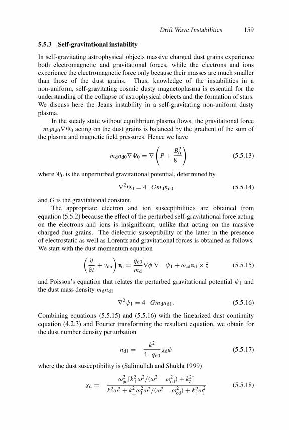
Drift Wave Instabilities 159
5.5.3 Self-gravitational instability
In self-gravitating astrophysical objects massive charged dust grains experienceboth electromagnetic and gravitational forces, while the electrons and ionsexperience the electromagnetic force only because their masses are much smallerthan those of the dust grains. Thus, knowledge of the instabilities in anon-uniform, self-gravitating cosmic dusty magnetoplasma is essential for theunderstanding of the collapse of astrophysical objects and the formation of stars.We discuss here the Jeans instability in a self-gravitating non-uniform dustyplasma.
In the steady state without equilibrium plasma flows, the gravitational force−mdnd0∇#0 acting on the dust grains is balanced by the gradient of the sum ofthe plasma and magnetic field pressures. Hence we have
−mdnd0∇#0 = ∇(
P + B20
8π
)(5.5.13)
where #0 is the unperturbed gravitational potential, determined by
∇2#0 = 4πGmdnd0 (5.5.14)
and G is the gravitational constant.The appropriate electron and ion susceptibilities are obtained from
equation (5.5.2) because the effect of the perturbed self-gravitational force actingon the electrons and ions is insignificant, unlike that acting on the massivecharged dust grains. The dielectric susceptibility of the latter in the presenceof electrostatic as well as Lorentz and gravitational forces is obtained as follows.We start with the dust momentum equation(
∂
∂ t+ νdn
)vd = qd0
md∇φ −∇ψ1 + ωcdvd × z (5.5.15)
and Poisson’s equation that relates the perturbed gravitational potential ψ1 andthe dust mass density mdnd1
∇2ψ1 = 4πGmdnd1. (5.5.16)
Combining equations (5.5.15) and (5.5.16) with the linearized dust continuityequation (4.2.3) and Fourier transforming the resultant equation, we obtain forthe dust number density perturbation
nd1 = − k2
4πqd0χdφ (5.5.17)
where the dust susceptibility is (Salimullah and Shukla 1999)
χd = −ω2
pd[k2⊥ω2/(ω2 − ω2cd)+ k2
z ]k2ω2 + k2⊥ω2
Jω2/(ω2 − ω2
cd)+ k2zω
2J
(5.5.18)
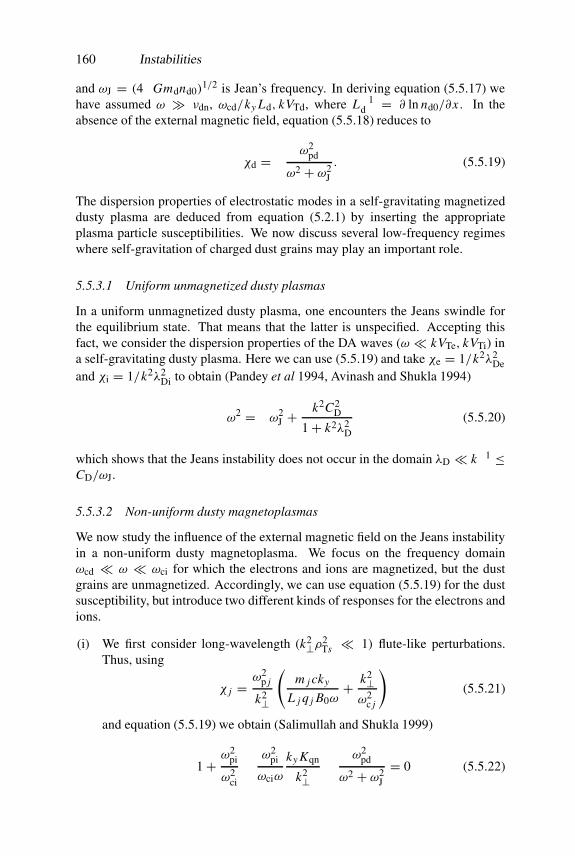
160 Instabilities
and ωJ = (4πGmdnd0)1/2 is Jean’s frequency. In deriving equation (5.5.17) we
have assumed ω � νdn, ωcd/ky Ld, kVTd, where L−1d = ∂ ln nd0/∂x . In the
absence of the external magnetic field, equation (5.5.18) reduces to
χd = −ω2
pd
ω2 + ω2J
. (5.5.19)
The dispersion properties of electrostatic modes in a self-gravitating magnetizeddusty plasma are deduced from equation (5.2.1) by inserting the appropriateplasma particle susceptibilities. We now discuss several low-frequency regimeswhere self-gravitation of charged dust grains may play an important role.
5.5.3.1 Uniform unmagnetized dusty plasmas
In a uniform unmagnetized dusty plasma, one encounters the Jeans swindle forthe equilibrium state. That means that the latter is unspecified. Accepting thisfact, we consider the dispersion properties of the DA waves (ω � kVTe, kVTi) ina self-gravitating dusty plasma. Here we can use (5.5.19) and take χe = 1/k2λ2
Deand χi = 1/k2λ2
Di to obtain (Pandey et al 1994, Avinash and Shukla 1994)
ω2 = −ω2J +
k2C2D
1+ k2λ2D
(5.5.20)
which shows that the Jeans instability does not occur in the domain λD � k−1 ≤CD/ωJ.
5.5.3.2 Non-uniform dusty magnetoplasmas
We now study the influence of the external magnetic field on the Jeans instabilityin a non-uniform dusty magnetoplasma. We focus on the frequency domainωcd � ω � ωci for which the electrons and ions are magnetized, but the dustgrains are unmagnetized. Accordingly, we can use equation (5.5.19) for the dustsusceptibility, but introduce two different kinds of responses for the electrons andions.
(i) We first consider long-wavelength (k2⊥ρ2Ts � 1) flute-like perturbations.
Thus, using
χ j =ω2
p j
k2⊥
(m j cky
L j q j B0ω+ k2⊥
ω2c j
)(5.5.21)
and equation (5.5.19) we obtain (Salimullah and Shukla 1999)
1+ ω2pi
ω2ci
− ω2pi
ωciω
ky Kqn
k2⊥− ω2
pd
ω2 + ω2J
= 0 (5.5.22)

Parametric Instabilities 161
where Kqn = (eni0)−1∂(qd0nd0)/∂x . Equation (5.5.22) can be rewritten as
(ω2 + ω2J )(ω − ωsv)− ω2
DHω = 0 (5.5.23)
which exhibits a coupling between the Jeans and Shukla–Varma modes. Wehave denoted ωDH = ωpdωci/ωpi and assumed ωpi � ωci. The effectsof the external magnetic field as well as of the density and dust chargeinhomogeneities can be deduced by numerically analysing equation (5.5.23).However, for ω � ωsv the latter yields ω2 = −ω2
J +ω2DH, which shows that
the magnetic field stabilizes the purely growing Jeans instability.(ii) We next consider the effects of finite kz on waves in a warm dusty plasma.
Considering the frequency regime kVTi, kzCS, ωcd � ω � kz VTe, ωci,we use the appropriate electron and ion susceptibilities (e.g. those givenin equations (5.5.1) and (5.5.3)) along with equation (5.5.19) to obtain(Salimullah and Shukla 1999)
(ω2 + ω2J )(ω − ωd∗)− ω2
seω = 0 (5.5.24)
which exhibits a coupling between the Jeans and dust drift modes. Here wehave denoted ωd∗ = (ni0Te/ne0Ti)ωi∗/(1+ k2
yρ2s ) and ωse = kλDeωpd/(1+
k2yρ
2s )
1/2. The effects of the external magnetic field and the ion densitygradient can be found by numerically analysing equation (5.5.24). Finally,we mention that inclusion of dust–neutral collisions in the above analysisyields a new resistive Jeans instability, as discussed by Shukla and Verheest(1999).
5.6 Parametric Instabilities
We have described numerous instabilities in the presence of streaming of plasmaparticles, ion drag force, as well as dust charge, plasma number density and ionflow gradients, etc. We now wish to discuss a few examples of the parametricinstabilities in the presence of large-amplitude electromagnetic (EM) waves in anunmagnetized dusty plasma.
5.6.1 Modulational interactions
We consider the nonlinear interaction between large-amplitude EM waves and theDA waves in a dusty plasma. The nonlinear equation for coherent EM waves inthe presence of DA waves is obtained from
∇ × B = 4π
cJ + 1
c
∂E∂ t
(5.6.1)
with B = ∇ × A, E = −∂ A/∂ t and J = −e(ne0 + ne1)ve, where ne1 isthe electron number density perturbation associated with the DA waves and the
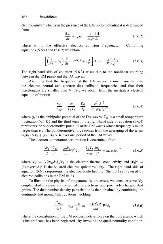
162 Instabilities
electron quiver velocity in the presence of the EM vector potential A is determinedfrom
∂ve
∂ t+ νeve = e
mec
∂ A∂ t
(5.6.2)
where νe is the effective electron collision frequency. Combiningequations (5.6.1) and (5.6.2) we obtain
[(∂
∂ t+ νe
)∂
∂ t− c2∇2 + ω2
pe
]A = −ω2
pene1
ne0A. (5.6.3)
The right-hand side of equation (5.6.3) arises due to the nonlinear couplingbetween the EM pump and the DA waves.
Assuming that the frequency of the DA waves is much smaller thanthe electron–neutral and electron–dust collision frequencies and that theirwavelengths are smaller than VTe/νe, we obtain from the inertialess electronequation of motion
ne1
ne0= eφs
kBTe− Te1
Te− e2|A|2
2mekBTec2 (5.6.4)
where φs is the ambipolar potential of the DA waves, Te1 is a small temperaturefluctuation (� Te) and the third term in the right-hand side of equation (5.6.4)represents the ponderomotive potential of the EM waves whose frequency is muchlarger than νe. The ponderomotive force comes from the averaging of the termsmeve · ∇ve + (e/c)ve × B over one period of the EM waves.
The electron temperature perturbation is determined from
3kB
2
∂Te1
∂ t− χ0kB
ne0∇2Te1 − kBTe
ne0
∂ne1
∂ t= meνe|ve|2 (5.6.5)
where χ0 = 3.2ne0V 2Te/νe is the electron thermal conductivity and |ve|2 =
(e/mec)2|A|2 is the squared electron quiver velocity. The right-hand side ofequation (5.6.5) represents the electron Joule heating (Stenflo 1985) caused byelectron collisions in the EM fields.
To illustrate the physics of the parametric processes, we consider a weaklycoupled dusty plasma composed of the electrons and positively charged dustgrains. The dust number density perturbation is then obtained by combining thecontinuity and momentum equations, yielding
∂2nd1
∂ t2+ νdn
∂nd1
∂ t= −nd0 Zd0e
md∇2φs (5.6.6)
where the contribution of the EM ponderomotive force on the dust grains, whichis insignificant, has been neglected. By invoking the quasi-neutrality condition,

Parametric Instabilities 163
namely Zd0nd1 = ne1, we can combine equations (5.6.4)–(5.6.6) to obtain(Shukla and Stenflo 2001a)[(
∂
∂ t− 2χ0
3ne0∇2)(
∂2
∂ t2+ νdn
∂
∂ t− C2
De∇2
)− 2
3C2
De∇2 ∂
∂ t
]ne1
ne0
= C2Deω
2pe
8πne0kBTec2
(∂
∂ t− 2χ0
3ne∇2 + 4
3νe
)∇2|A|2 (5.6.7)
which is the DA wave equation in the presence of the radiation pressure and thethermal nonlinearity produced by the differential Joule heating of electrons in thepresence of EM waves. Here CDe = ωpdλDe is the DA speed in a positive dust–electron plasma (Shukla 2000a, c).
We consider the parametric excitation of the DA waves by EM waves. Letus suppose that an EM pump, A0 exp(−iω0t + ik0 · r) + complex conjugate,interacting with low-frequency (ω (� ω0), k) DA waves generates EM sidebandsA± exp(−iω±t+ik±·r), whereω± = ω±ω0 and k± = k±k0 are the frequenciesand wavenumbers for the EM sidebands. Hence we obtain from (5.6.3) and (5.6.7)after Fourier transformation and matching the phasors
D±A± = ω2pe N A0± (5.6.8)
and
[(ω + iωχ)εl − 23ωω
2d]N
= ω2deω
2pe
8πne0kBTec2
(ω + iωχ + i
4
3νe
)(A0− · A+ + A0+ · A−) (5.6.9)
where D± = ω±(ω± + iνe) − ω2pe − k2±c2, εl = ω(ω + iνdn) − ω2
de, ωde =kCDe, ωχ = 2k2χe/3ne0, N = ne1/ne0, ne1 = ne1 exp(−iωt + ik · r),A0+ = A0, A0− = A∗0 and the asterisk denotes the complex conjugate. Fromequations (5.6.8) and (5.6.9) we readily obtain the nonlinear dispersion relation(Shukla and Stenflo 2001)
(ω + iωχ)εl − 2
3ωω2
de =(ω + iωχ + i
4νe
3
)ω2
deω4pe
W0
c2
∑±
ε−1± (5.6.10)
where W0 = |A0|2/8πne0kBTe. Note that ε± ≈ ±2ω0(ω + i�e − k · vg ∓ δe),where vg ≈ kc2/ω0 is the group velocity of the pump, ω0 = (k2
0c2 + ω2pe)
1/2
is the pump wave frequency, �e = νeω2pe/2ω0 is the collisional damping rate of
the EM waves and δe = k2c2/2ω0 is the frequency shift caused by the nonlinearinteraction of the EM waves with the DA waves. The pump and sidebands areassumed to be coplanar.
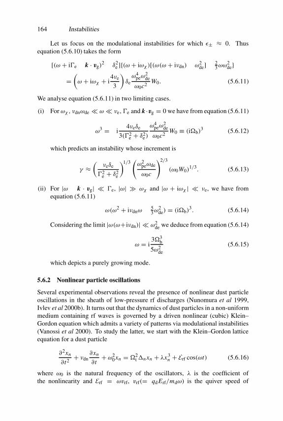
164 Instabilities
Let us focus on the modulational instabilities for which ε± ≈ 0. Thusequation (5.6.10) takes the form
[(ω + i�e − k · vg)2 − δ2
e ]{(ω + iωχ)[(ω(ω + iνdn)− ω2de] − 2
3ωω2de}
=(ω + iωχ + i
4νe
3
)δeω4
peω2de
ω0c2W0. (5.6.11)
We analyse equation (5.6.11) in two limiting cases.
(i) For ωχ, νdnωde � ω � νe, �e and k ·vg = 0 we have from equation (5.6.11)
ω3 = −i4νeδe
3(�2e + δ2
e )
ω4peω
2de
ω0c2W0 ≡ (i�b)
3 (5.6.12)
which predicts an instability whose increment is
γ ≈(
νeδe
�2e + δ2
e
)1/3(ω2
peωde
ω0c
)2/3
(ω0W0)1/3. (5.6.13)
(ii) For |ω − k · vg| � �e, |ω| � ωχ and |ω + iωχ | � νe, we have fromequation (5.6.11)
ω(ω2 + iνdnω − 53ω
2de) = (i�b)
3. (5.6.14)
Considering the limit |ω(ω+iνdn)| � ω2de we deduce from equation (5.6.14)
ω = i3�3
b
5ω2de
(5.6.15)
which depicts a purely growing mode.
5.6.2 Nonlinear particle oscillations
Several experimental observations reveal the presence of nonlinear dust particleoscillations in the sheath of low-pressure rf discharges (Nunomura et al 1999,Ivlev et al 2000b). It turns out that the dynamics of dust particles in a non-uniformmedium containing rf waves is governed by a driven nonlinear (cubic) Klein–Gordon equation which admits a variety of patterns via modulational instabilities(Vanossi et al 2000). To study the latter, we start with the Klein–Gordon latticeequation for a dust particle
∂2xn
∂ t2+ νdn
∂xn
∂ t+ ω2
0xn = �2t �nxn + λx3
n + Erf cos(ωt) (5.6.16)
where ω0 is the natural frequency of the oscillators, λ is the coefficient ofthe nonlinearity and Erf = ωvrf, vrf(= qd Erf/mdω) is the quiver speed of

Parametric Instabilities 165
the dust particle in the rf field Erf cos(ωt). The nearest-neighbour coupling is�nxn = 2xn − xn+1 − xn−1. The origin of the nonlinear term λx3
n in a dustyplasma sheath is not yet fully understood, although Ivlev et al (2000b) suggestthat it could be associated with the change in the electrostatic energy of theparticles. However, in the presence of dust charge fluctuations we may deduce theparameter λ = (E0/md)(∂
3qd0/∂x3n)xn=x0 , by assuming (∂2qd0/∂x2)xn=x0 = 0,
and thereby ignoring the quadratic term. The properties of equation (5.6.16) havebeen rigorously analysed in textbooks (e.g. Landau and Lifshitz 1960, Nayfehand Mook 1979). We now seek a solution of equation (5.6.16) in the formxn = xn0 cos(ωt + δc) within the rotating frame approximation. The amplitudexn0 and phase δc of the spatially homogeneous solution satisfy
x2n0[ν2
dnω2 + (ω2 − ω2
0 + 34λx2
n0)2] = E
2rf (5.6.17)
which admits two classes of solutions (Vanossi et al 2000) for the amplitude xn0of the response to a driving amplitude Erf. The solutions depend on the values ofω/ω0, νdn/ω0 and λ.
Let us analyse the modulational stability of the homogenous solution againstspatial perturbations of the form xn = y + zn . Assuming periodic boundaryconditions, we may expand zn = ∑k exp(ikn)ξk(t), where the mode amplitudeξk(t) is governed by (Vanossi et al 2000)
∂2ξk
∂ t2 + νdn∂ξk
∂ t+ ω2
kξk = 3
2λx2
n0[1+ cos(2ωt + 2δc)]ξk (5.6.18)
where ω2k = ω2
0 + 4�2t sin2(k/2) denotes the linear dispersion relation of the
system. The transformation ξk(t) = ξk(ωt + δc) exp[−(νdn/2ω)(ωt + δc)] ≡ξk(τ ) exp[−(νdn/2ω)τ ] reduces equation (5.6.18) to a standard Mathieu equation
d2ξk
dτ 2+ acξk − 2bc cos(2τ )ξk = 0 (5.6.19)
where
ac = 1
4ω2 (4ω2k − 6λx2
n0 − ν2dn) and bc = 3λx2
n0
4ω2 . (5.6.20)
It is well known that equation (5.6.19) exhibits parametric resonances when√ac = j , where j = 1, 2, 3 . . . . The width of the resonance depends on the
ratio bc/ac. The extent of the primary resonance ac � 1 can easily be estimatedto be (ac − 1)2 < b2
c . However, in the presence of the damping νdn the resonancecondition for equation (5.6.18) becomes
b2c >
ν2dn
ω2+ (ac − 1)2. (5.6.21)
Vanossi et al (2000) have presented a stability diagram showing the stabilityboundaries between the possible patterns in the (Erf, k) plane. The modulational
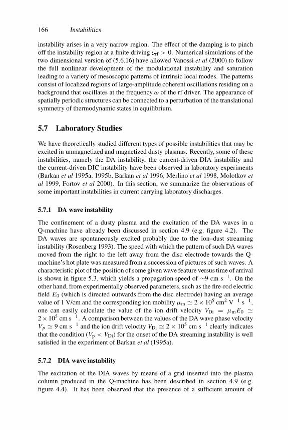
166 Instabilities
instability arises in a very narrow region. The effect of the damping is to pinchoff the instability region at a finite driving Erf > 0. Numerical simulations of thetwo-dimensional version of (5.6.16) have allowed Vanossi et al (2000) to followthe full nonlinear development of the modulational instability and saturationleading to a variety of mesoscopic patterns of intrinsic local modes. The patternsconsist of localized regions of large-amplitude coherent oscillations residing on abackground that oscillates at the frequency ω of the rf driver. The appearance ofspatially periodic structures can be connected to a perturbation of the translationalsymmetry of thermodynamic states in equilibrium.
5.7 Laboratory Studies
We have theoretically studied different types of possible instabilities that may beexcited in unmagnetized and magnetized dusty plasmas. Recently, some of theseinstabilities, namely the DA instability, the current-driven DIA instability andthe current-driven DIC instability have been observed in laboratory experiments(Barkan et al 1995a, 1995b, Barkan et al 1996, Merlino et al 1998, Molotkov etal 1999, Fortov et al 2000). In this section, we summarize the observations ofsome important instabilities in current carrying laboratory discharges.
5.7.1 DA wave instability
The confinement of a dusty plasma and the excitation of the DA waves in aQ-machine have already been discussed in section 4.9 (e.g. figure 4.2). TheDA waves are spontaneously excited probably due to the ion–dust streaminginstability (Rosenberg 1993). The speed with which the pattern of such DA wavesmoved from the right to the left away from the disc electrode towards the Q-machine’s hot plate was measured from a succession of pictures of such waves. Acharacteristic plot of the position of some given wave feature versus time of arrivalis shown in figure 5.3, which yields a propagation speed of ∼9 cm s−1. On theother hand, from experimentally observed parameters, such as the fire-rod electricfield E0 (which is directed outwards from the disc electrode) having an averagevalue of 1 V/cm and the corresponding ion mobility µm � 2× 105 cm2 V−1 s−1,one can easily calculate the value of the ion drift velocity VDi = µm E0 �2×105 cm s−1. A comparison between the values of the DA wave phase velocityVp � 9 cm s−1 and the ion drift velocity VDi � 2× 105 cm s−1 clearly indicatesthat the condition (Vp < VDi) for the onset of the DA streaming instability is wellsatisfied in the experiment of Barkan et al (1995a).
5.7.2 DIA wave instability
The excitation of the DIA waves by means of a grid inserted into the plasmacolumn produced in the Q-machine has been described in section 4.9 (e.g.figure 4.4). It has been observed that the presence of a sufficient amount of
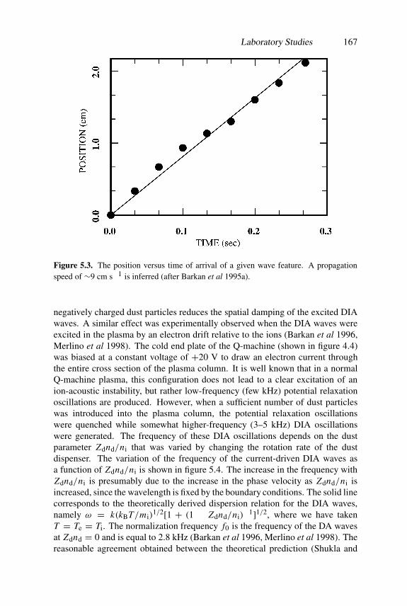
Laboratory Studies 167
Figure 5.3. The position versus time of arrival of a given wave feature. A propagationspeed of ∼9 cm s−1 is inferred (after Barkan et al 1995a).
negatively charged dust particles reduces the spatial damping of the excited DIAwaves. A similar effect was experimentally observed when the DIA waves wereexcited in the plasma by an electron drift relative to the ions (Barkan et al 1996,Merlino et al 1998). The cold end plate of the Q-machine (shown in figure 4.4)was biased at a constant voltage of +20 V to draw an electron current throughthe entire cross section of the plasma column. It is well known that in a normalQ-machine plasma, this configuration does not lead to a clear excitation of anion-acoustic instability, but rather low-frequency (few kHz) potential relaxationoscillations are produced. However, when a sufficient number of dust particleswas introduced into the plasma column, the potential relaxation oscillationswere quenched while somewhat higher-frequency (3–5 kHz) DIA oscillationswere generated. The frequency of these DIA oscillations depends on the dustparameter Zdnd/ni that was varied by changing the rotation rate of the dustdispenser. The variation of the frequency of the current-driven DIA waves asa function of Zdnd/ni is shown in figure 5.4. The increase in the frequency withZdnd/ni is presumably due to the increase in the phase velocity as Zdnd/ni isincreased, since the wavelength is fixed by the boundary conditions. The solid linecorresponds to the theoretically derived dispersion relation for the DIA waves,namely ω = k(kBT/mi)
1/2[1 + (1 − Zdnd/ni)−1]1/2, where we have taken
T = Te = Ti. The normalization frequency f0 is the frequency of the DA wavesat Zdnd = 0 and is equal to 2.8 kHz (Barkan et al 1996, Merlino et al 1998). Thereasonable agreement obtained between the theoretical prediction (Shukla and

168 Instabilities
Figure 5.4. The variation of the frequency of the current-driven DIA waves as a functionof Zdnd/ni. The open circles correspond to laboratory measurements (after Merlino et al1998), whereas the solid line corresponds to the theoretically derived dispersion relation(Shukla and Silin 1992) for the DIA waves.
Silin 1992) and the experimental results supports the identification of the sourceof the oscillations.
5.7.3 EIC instability
The EIC instability is produced by drawing an electron current along the axisof the plasma column to a 5 mm diameter disc located near the end of the dustdispenser far away from the hot plate of the DPD machine shown in figure 1.8.A disc bias (0.5–1 V) above the space potential produces an electron driftsufficient to excite electrostatic waves with a frequency slightly above the iongyrofrequency, which propagate radially outwards from the current channel witha wavevector that is nearly perpendicular to the magnetic field. To study the effectof the dust on the instability, the wave amplitude A0 without the dust particle wasmeasured, and without introducing any other changes in the plasma conditions thedust dispenser was turned on and the wave amplitude Ad and the correspondingZdnd/ni were measured in the presence of the dust particles (Barkan et al 1995b,Merlino et al 1998). The ratio Ad/A0 could then be used as an indication of theeffect of the dust. This procedure was repeated for various dust dispenser rotationrates. The results of these measurements are shown in figure 5.5. It appears thatas more and more electrons attach onto the dust grains, i.e. Zdnd increases, itbecomes increasingly easier to excite the EIC waves in the sense that for a given
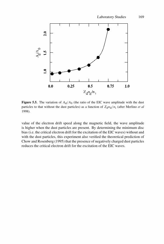
Laboratory Studies 169
Figure 5.5. The variation of Ad/A0 (the ratio of the EIC wave amplitude with the dustparticles to that without the dust particles) as a function of Zdnd/ni (after Merlino et al1998).
value of the electron drift speed along the magnetic field, the wave amplitudeis higher when the dust particles are present. By determining the minimum discbias (i.e. the critical electron drift for the excitation of the EIC waves) without andwith the dust particles, this experiment also verified the theoretical prediction ofChow and Rosenberg (1995) that the presence of negatively charged dust particlesreduces the critical electron drift for the excitation of the EIC waves.
Chapter 6
Elongated Dust Grains
6.1 Introduction
Elongated charged dust grains are ubiquitous in cosmic (Spitzer 1977, Harwit1988) and laboratory plasmas (Chu and I 1994, Mohideen et al 1998, Rahmanet al 2001). The formation of elongated charged dust grains is attributed tothe coagulation of particulates in partially or fully ionized gases. Elongatedcharged grains can acquire rotational and spinning motions due to their interactionwith photons and particles of the surrounding gas or due to the presence ofan oscillating electric field in a plasma (Tskhakaya and Shukla 2001). Inastrophysical objects the angular frequency of the dust grain rotation can reach arather large value, namely between tens of kHz to MHz for thermal dust grains andhundreds and thousands of MHz for super-thermal grains (Spitzer 1977, Harwit1988). Furthermore, recent laboratory experiments use cylindrical macroscopicgrains in studies of ordered structures (Molotkov et al 2000) and levitation ofmicro-rods in the collisional sheath of an rf plasma (Annaratone et al 2001).
In this chapter, we discuss the electrodynamics (Tskhakaya et al 2001) anddispersion properties of a dusty magnetoplasma whose constituents are electrons,ions and finite-sized elongated dust grains. Specifically, we develop expressionsfor the charge and current densities for elongated dust grains by including theeffects of the dust dipole moment and the dust grain rotation. The forcesacting on the dust grains as well as the corresponding dust kinetic equationand the equations of motion are deduced. The dispersion relations for bothelectromagnetic and electrostatic waves are obtained and analysed. The rotationaldust grain energy can be coupled to the various dusty plasma modes. Alsodescribed are some mechanisms which are responsible for bouncing, vibrational(quivering) and rotational motions of charged dust grains in a dusty plasma.
170
Dust Charge and Current Densities 171
6.2 Dust Charge and Current Densities
Let us consider a multi-component dusty plasma in an external magnetic fieldzB0. The dusty plasma constituents are electrons, ions and negatively chargednon-spherical rotating dust grains. To construct the electrodynamics of elongatedcharged dust grains in a magnetized dusty plasma, we have to obtain appropriateexpressions for the charge and current densities of dust grains through a dustgrain distribution function, taking into account the size of the dust grains. For ourpurposes, we assume that the charged dust grains form a system of discrete parts(Landau and Lifshitz 1971). The charge microdensity of the grains is representedas
ρm =∑
i
[∑j
dqi (r j )δ(r − r j )
](6.2.1)
where the first summation over i is taken over different grains, while the secondover j is taken over different parts of the i th grain, as shown in figure 6.1. Heredqi (r j ) is the charge of the j th part of the i th grain and δ(r − r j ) is the usualDirac delta function. If there is a continuous charge distribution onto the grain,the summation over j can be changed by an integral over the grain’s volume andthe density of the charge onto the dust grain can be written as
ρm =∑
i
∫Vi (Ri )
ρi (r ′ − Ri , Ri )δ(r − r ′) (6.2.2)
where Ri is the radius vector of the centre of mass of the grain and the integral istaken over the volume Vi (Ri) of the grain. In equation (6.2.2) we introduced thedensity of the charge distribution onto the grain as
dqi (r) = dqi(r)dr
dr ≡ ρi (r − Ri , Ri ) dr. (6.2.3)
For a point grain charge, we have
ρi (r − Ri , Ri ) = qiδ(r − Ri ) (6.2.4)
which leads to the usual expression for the charge microdensity of the grain
ρm =∑
i
qiδ(r − Ri ) (6.2.5)
where qi is the total charge of the i th grain.To present a statistical description of the dust grain gas, we have to introduce
the probability density D for the grain’s gas state (Landau and Lifshitz 1971,Klimontovich 1982). If all grains are identical, we have
D = D(R1, v1,�1, θ1, ψ1, ϕ1; R2, v2,�2, θ2, ψ2, ϕ2; . . . , t) (6.2.6)
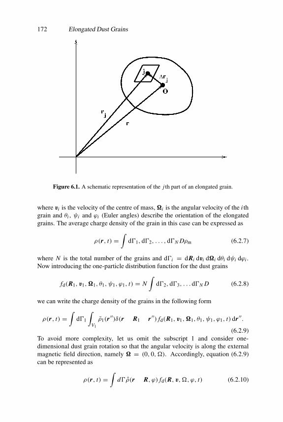
172 Elongated Dust Grains
Figure 6.1. A schematic representation of the j th part of an elongated grain.
where vi is the velocity of the centre of mass, �i is the angular velocity of the i thgrain and θi , ψi and ϕi (Euler angles) describe the orientation of the elongatedgrains. The average charge density of the grain in this case can be expressed as
ρ(r, t) =∫
d�1, d�2, . . . , d�N Dρm (6.2.7)
where N is the total number of the grains and d�i = dRi dvi d�i dθi dψi dϕi .Now introducing the one-particle distribution function for the dust grains
fd(R1, v1,�1, θ1, ψ1, ϕ1, t) = N∫
d�2, d�3, . . . d�N D (6.2.8)
we can write the charge density of the grains in the following form
ρ(r, t) =∫
d�1
∫V1
ρ1(r ′′)δ(r − R1 − r ′′) fd(R1, v1,�1, θ1, ψ1, ϕ1, t) dr ′′.
(6.2.9)To avoid more complexity, let us omit the subscript 1 and consider one-dimensional dust grain rotation so that the angular velocity is along the externalmagnetic field direction, namely � = (0, 0,�). Accordingly, equation (6.2.9)can be represented as
ρ(r, t) =∫
d�ρ(r − R, ϕ) fd(R, v,�, ϕ, t) (6.2.10)
Dust Charge and Current Densities 173
where the integrand
ρ(r − R, ϕ) =∫
Vdr ′ ρ(r ′)δ(r − R − r ′) (6.2.11)
describing the charge distribution onto a single grain depends on the shape of thegrain and the azimuthal orientation of the grain’s elongation axis. Outside of thegrain’s volume, we have ρ = 0. For identical grains, we can partly determine thedependence of ρ on the azimuthal angle ϕ. Every given direction of the grain’selongation axis, determined by the angle ϕ, can be considered as a final position ofthe turning of the axis (and simultaneously of the whole grain) from the directionwith ϕ = 0. This allows us to write
ρ(r − R, ϕ) = ρ[↔F (ϕ)(r − R), 0] ≡ ρ[↔F (ϕ)(r − R)] (6.2.12)
where↔F (ϕ) is the tensor of turning by the angle ϕ, namely
↔F= Fij (ϕ) =
(cosϕ − sinϕsin ϕ cosϕ
). (6.2.13)
In the dipole approximation, when the dust grain size rd is much smaller than thescalelength of the plasma inhomogeneity λin, namely
rd � λin (6.2.14)
we substitute equation (6.2.12) into equation (6.2.10) and expand the distributionfunction fd around the point r and obtain for the grain’s charge density
ρd(r, t) =∫(q − d · ∇) fd(r, v,�, ϕ, t) d' (6.2.15)
where d' = dv d� dϕ,
q =∫
dr ρ(r) (6.2.16)
and
d =↔F −1(ϕ)
∫dr rρ(r) (6.2.17)
are the total charge and the dipole moment of the dust grain, respectively, and↔F −1 is the inverse of the tensor
↔F (ϕ). An analogous calculation leads to the
following expression for the dust current density (Tskhakaya et al 2001)
Jd(r, t) =∫
d' [v(q − d · ∇)+�× d] fd(r, v,�, ϕ, t). (6.2.18)
The first term in the right-hand side of equation (6.2.18) describes the transfer ofthe charge (6.2.15) and the second term describes the current arising from the dustgrain rotation.

174 Elongated Dust Grains
6.3 Grain Kinetic Equation
To construct a kinetic equation for the elongated dust grains, we should have acomplete knowledge of the forces that act on the dust grains in the presence ofelectromagnetic fields. Supposing that charged dust grains constitute a discretesystem of particles, we have for the Lagrangian (Tskhakaya et al 2001)
L =∑
i
�mi u2i
2+ 1
c
∑i
�qi [vi · A(ri , t)] −∑
i
�qiφ(ri , t) (6.3.1)
where �mi and �qi are the mass and the charge of the i th grain, respectively, ri
and ui are its position and velocity. Separating the motions of the centre of massand the rotation around it, we can write ui = v+��ri and ri = r+�ri , wherev and ri are the velocity and position of the centre of mass, �ri is the coordinateof the i th part of the grain relative to the centre of mass and � is the angularvelocity of the dust grain. The dipole approximation (namely equation (6.2.14))allows us to expand the potentials as
A(ri , t) = A(ri , t)+ (�ri · ∇)A(ri , t) + 12 (�ri · ∇)2 A(ri , t)+ · · · (6.3.2)
and
φ(ri , t) = φ(ri , t)+ (�ri · ∇)φ(r, t)+ 12 (�ri · ∇)2φ(r, t)+ · · · . (6.3.3)
Accordingly, the Lagrangian (6.3.1) becomes
L = mdv2
2+ 1
2Iαβ�α�β + q
cv · A(ri , t)− qφ(ri , t)+ m · B
+[
d + 1
2
∑i
�qi�ri (�ri · ∇)]·(
E + v
c× B
)(6.3.4)
where md = ∑i �mi and q = ∑i �qi are the total mass and the charge of thegrain, respectively, Iα,β = ∑i �mi [(�ri)
2δαβ − (�ri )α · (�ri )β ] is the tensorof the moment of inertia, d =∑i �qi�ri is the dipole moment of the elongatedgrain and m = (1/2c)
∑i �qi(�ri × Ui ) is the magnetic moment of the grain.
Here Ui = �×�ri is the rotational velocity. The electric and magnetic fields areE = −∇φ − c−1∂ A(ri , t)/∂ t and B = ∇ × A(ri , t), respectively. In deriving(6.3.4), we used the relation
dddt= �× d. (6.3.5)
Note that in the presence of the gravitational field g, we must add the term md g ·ri
in the right-hand side of equation (6.3.4). We neglect the second term (which isassociated with the multi-dipole effect) in the square bracket of equation (6.3.4)and obtain the equations of motion for the elongated dust grains as
d pdt= (q + d · ∇)
(E + 1
cv × B
)+ 1
c(�× d)× B + (m× ∇)× B (6.3.6)

Dielectric Permittivity 175
and
dMα
dt= −1
2Sαβ
[∂Bβ
∂ t+ (v · ∇)Bβ
]+[
d ×(
E + 1
cv × B
)]α
+ (m × B)α
(6.3.7)where p = mdv, Sαβ = c−1∑
i �qi [(�ri)2δαβ − (�ri )α(�ri )β ] and Mα =
Iαβ�β is the angular momentum of the grain. The kinetic equation for theelongated dust grains can now be written as
∂ fd
∂ t+ v · ∂ fd
∂ r+� · ∂ fd
∂ϕ+ d p
dt· ∂ fd
∂ p+ dM
dt· ∂ fd
∂M= 0. (6.3.8)
It can be easily shown from equations (6.3.8), (6.2.15) and (6.2.18) that the dustgrain charge and current densities satisfy the continuity equation
∂ρd
∂ t+∇ · Jd = 0. (6.3.9)
We can, therefore, construct the kinetics and electrodynamics of a dusty plasmawith elongated and rotating dust grains by means of the expressions for ρd andJd.
6.4 Dielectric Permittivity
We assume that the dust grain size is much smaller than the grain gyroradius andthat the dust grain thermal speed is smaller than the characteristic speed of ourproblem. Under these conditions along with equation (6.2.14), the equations ofmotion (6.3.6) and (6.3.7) can be simplified. We consider the one-dimensionalcase of dust grain rotation so that M = (0, 0, M), where M = I� and I is thez component of the principal moment of inertia. The kinetic equation (6.3.8) forthe dust grain then takes the form
∂ fd
∂ t+ v · ∂ fd
∂ r+�
∂ fd
∂ϕ+ (d × E)z
∂ fd
∂M+ q
(E + 1
cv × B
)· ∂ fd
∂ p= 0. (6.4.1)
The well known kinetic equations for the electrons and ions are
∂ f j
∂ t+ v · ∂ f j
∂ r+ q j
(E + 1
cv × B
)· ∂ f j
∂ p= 0. (6.4.2)
Now assuming that the wave electric and magnetic field perturbations are small,we can express the perturbed distribution function as δ fs = fs − fs0 � fs0. Theequilibrium distribution functions are of the form (Landau and Lifshitz 1989)
fd0 = nd0
2π(2πmdkBTd)3/2
1
(2π I kBTd)1/2
× exp[−(p2/2mdkBTd)− (M − M0)2/2I kBTd] (6.4.3)
176 Elongated Dust Grains
andf j0 = n j0
(2πm j kBTj )3/2exp[−(p2/2m j kBTj )]. (6.4.4)
We assumed that the dust grains rotate with a preferred angular velocity �0 sothat M0 = I�0. The components of the dust dipole moment are
dx = d cosϕ, dy = d sinϕ. (6.4.5)
Thus, the perturbed dust grain distribution function is represented as
δ fd =∞∑
n=−∞δ fn exp(inϕ). (6.4.6)
6.4.1 Unmagnetized dusty plasmas
We first consider an unmagnetized dusty plasma (B0 = 0) and assume that allperturbed quantities are proportional to exp(−iωt + ik · r). We linearize (6.4.1)and (6.4.2) and substitute them into the Poisson–Maxwell equations and obtainthe dielectric tensor for the dusty plasma following the standard method. Theresult is (Alexandrov et al 1984)
εi j (ω, k) = kik j
k2εl(ω, k) +
(δi j − ki k j
k2
)εt(ω, k) +
(δi j − �i� j
�2
)εd(ω, k)
(6.4.7)where εl(ω, k) and εt(ω, k) are the usual longitudinal and transverse dielectricpermittivities, respectively. They are given by
εl(ω, k) = 1+∑
s
ω2ps
k2V 2Ts
[1− J+
(ω
kVTs
)](6.4.8)
and
εt(ω, k) = 1−∑
s
ω2ps
ω2J+(
ω
kVTs
). (6.4.9)
The function J+(x) is
J+(x) = x√2π
∫ ∞
−∞dz
exp(−z2/2)
x − z. (6.4.10)
The asymptotic forms of equation (6.4.10) are
J+(x) ≈ 1+ 1
x2 + · · · − i
√π
2x exp
(− x2
2
)(6.4.11)
for |x | � 1, |Re x | � | Im x |, Im x < 0 and
J+(x) ≈ −i
√π
2x (6.4.12)

Dielectric Permittivity 177
for |x | � 1. The influence of the dust grain rotation is described by εd(ω, k),which is
εd(ω, k) = − �2r
ω2
k2
K 2
ω
ω −�0J+(ω −�0
K VTd
)
+ �2r
K 2V 2Td
(κ2
K 2+ k2
K 2
�0
ω
)[1− J+
(ω −�0
K VTd
)](6.4.13)
where �r = (4πd2nd0/4I )1/2, K = (k2 + κ2)1/2 and κ = (md/I )1/2.
6.4.2 Magnetized dusty plasmas
We now consider a magnetized dusty plasma (B0 �= 0). Here equations (6.4.1)and (6.4.2) for the dust grains read
∂δ fn
∂ t+ v · ∂δ fn
∂ r+ in�δ fn − ωcd
∂δ fn
∂ψa= −q E · ∂ fd0
∂ p�(n)
− i
2
∂ fd0
∂Md[(Ex − iEy)�(n − 1)− (Ex + iEy)�(n + 1)] (6.4.14)
while for the electrons and ions we have
∂δ f j
∂ t+ v · ∂δ f j
∂ r− ωcj
∂δ f j
∂ψa= −q j E · ∂ f j0
∂ p(6.4.15)
where ωcd = q B0/mdc, ωc j = q j B0/m j c and �(n) = 1 for n = 0 and 0for n �= 0. The symbol ψa is the azimuthal angle in the momentum space,px = p⊥ cosψa and py = p⊥ sinψa. According to equation (6.4.14) onlyn = 0,±1 give a contribution in the summation of equation (6.4.6).
Assuming that the perturbed quantities are proportional to exp(−iωt+ ik · r),we obtain the following solutions of equations (6.4.14) and (6.4.15)
δ f0 = qd Eωcd
·∫ ψa
±∞dψ ′ ∂ fd0
∂ pexp
{−∫ ψa
ψ ′
[�R(ψ
′′)ωcd
]dψ ′′
}(6.4.16)
δ f±1 = ± i
2
d E∓ωcd
∫ ψa
±∞dψ ′ ∂ fd0
∂Mexp
{−∫ ψa
ψ ′
[�R(ψ
′′)∓�
ωcd
]dψ ′′
}(6.4.17)
and
δ f j = q j E·ωcα
∫ ψa
±∞dψ ′
∂ f j0
∂ pexp
{−∫ ψa
ψ ′
[�R(ψ
′′)ωcj
]dψ ′′
}(6.4.18)
where �R(ψ′′) = ω − k · v(ψ ′′) and E∓ = Ex ∓ iEy . Substituting
equations (6.4.16)–(6.4.18) into equation (6.2.18) as well as the linearized version

178 Elongated Dust Grains
of equation (6.4.2) into the expression for the electron and ion current densities,namely
J j = q j
∫d p vδ f j (6.4.19)
we obtain for the total current density
Ji =[σ r
i j (ω, k) +∑
s=e,i,d
σ si j (ω, k)
]E j (6.4.20)
where the first term in the right-hand side of equation (6.4.20) is connected withthe rotation of the dust grain, while the second term represents the contributionsof the electrons and ions including the centre of mass motion of the grains. Wehave denoted
σ ri j (ω, k) =
(σ r
x x σ rxy 0
−σ rxy σ r
yy 00 0 0
)(6.4.21)
where (Tskhakaya et al 2001)
σ rx x = σ r
yy = ind0d2
4I
1
K VTd
∞∑n=−∞
�n(bd)($n− +$n+) (6.4.22)
σ rxy =
nd0d2
4I
1
K VTd
∞∑n=−∞
�n(bd)($n− −$n+) (6.4.23)
with
$n± =k2
z
K 2
K VTd
ω ±�0 − nωcdJ+(ω ±�0 − nωcd
K VTd
)
−(κ2
K 2
ω − nωcd
K VTd∓ k2
z
K 2
�0
K VTd
)[1+ J+
(ω ±�0 − nωcd
K VTd
)].
(6.4.24)
For the tensor σ si j (ω, k), we have
σi j (ω, k) = q2s
ωcs
∫d p vi (ψa)
∫ ψa
±∞dψ ′
(∂ fs0
∂p j
)ψ ′
× exp
{i∫ ψa
ψ ′
[�R(ψ
′′)ωcs
]dψ ′′
}. (6.4.25)
We now carry out straightforward calculations and obtain the expressions for thedifferent elements of the tensor of the dielectric permittivity (Alexandrov et al1984). We have
εi j (ω, k) = εi j (ω, k) + εri j (ω, k) (6.4.26)
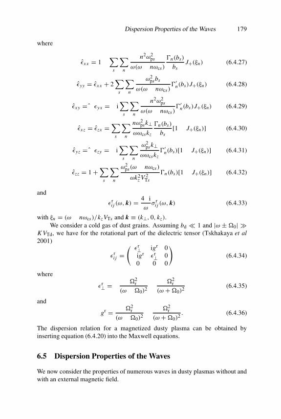
Dispersion Properties of the Waves 179
where
εx x = 1−∑
s
∑n
n2ω2ps
ω(ω − nωcs)
�n(bs)
bsJ+(ξn) (6.4.27)
εyy = εx x + 2∑
s
∑n
ω2psbs
ω(ω − nωcs)�′n(bs)J+(ξn) (6.4.28)
εxy = −εyx = −i∑
s
∑n
n2ω2ps
ω(ω − nωcs )�′n(bs)J+(ξn) (6.4.29)
εxz = εzx =∑
s
∑n
nω2psk⊥
ωωcskz
�n(bs)
bs[1− J+(ξn)] (6.4.30)
εyz = −εzy = −i∑
s
∑n
ω2psk⊥
ωωcskz�′n(bs)[1− J+(ξn)] (6.4.31)
εzz = 1+∑
s
∑n
ω2ps(ω − nωcs)
ωk2z V 2
Ts
�n(bs)[1− J+(ξn)] (6.4.32)
and
εri j (ω, k) = 4π i
ωσ r
i j (ω, k) (6.4.33)
with ξn = (ω − nωcs)/kz VTs and k ≡ (k⊥, 0, kz).We consider a cold gas of dust grains. Assuming bd � 1 and |ω ± �0| �
K VTd, we have for the rotational part of the dielectric tensor (Tskhakaya et al2001)
εri j =
(εr⊥ igr 0−igr εr⊥ 0
0 0 0
)(6.4.34)
where
εr⊥ = −�2
r
(ω −�0)2− �2
r
(ω +�0)2(6.4.35)
and
gr = �2r
(ω −�0)2− �2
r
(ω +�0)2. (6.4.36)
The dispersion relation for a magnetized dusty plasma can be obtained byinserting equation (6.4.20) into the Maxwell equations.
6.5 Dispersion Properties of the Waves
We now consider the properties of numerous waves in dusty plasmas without andwith an external magnetic field.

180 Elongated Dust Grains
6.5.1 Unmagnetized dusty plasmas
Let us consider the frequency regimes kVTd � ω � kVTi, kVTe and ω ± �0 �K VTd. Without loss of generality, we may assume that the wavevector k lies inthe (x, z) plane, i.e. k = (k⊥, 0, kz). In such a situation, the general dispersionrelation is of the form (Alexandrov et al 1984)∣∣∣∣∣k2δi j − ki k j − ω2
c2 εi j (ω, k)
∣∣∣∣∣ = 0. (6.5.1)
We now discuss two specific examples for wave phenomena associated with theelongated and rotating dust grains.
6.5.1.1 Transverse waves
We assume that the transverse waves under consideration are polarized along they-axis so that E = (0, E, 0). Thus, equation (6.5.1) gives
k2c2 + ω2pd
ω2= 1− 2�2
r
(ω −�0)2. (6.5.2)
For �0 = 0 the influence of the dust grain rotation disappears. However, forwaves with frequencies close to �0 (ωpd ≈ �r), we obtain
ω = �0
[1± i
√2�r
(k2c2 + ω2pd)
1/2
]. (6.5.3)
Equation (6.5.3) reveals that the ordinary transverse waves become unstable. Thegrowth rate is given by
√2�0�r/(k2c2 + ω2
pd)1/2, which strongly depends upon
�r (which is a function of the dipole moment as well as the moment of inertia ofthe dust grains) and the dust rotation frequency �0. It is worth noting that in theplasma without the dust grains, the low-frequency transverse oscillations decayaperiodically due to their collisionless absorption by the electrons.
6.5.1.2 Longitudinal waves
Equation (6.5.1) also admits low-frequency (|ω| � kc, kVTe, kVTi, |ω − �0| �K VTd) longitudinal waves. We consider two cases.
(i) DA waves
The modified dispersion relation for the DA waves (Rao et al 1990), which isdeduced from equation (6.5.1) by using the appropriate susceptibilities, reads(Mahmoodi et al 2000)
1+ 1
k2λ2D
− ω2pd
ω2 −k2⊥k2
[�2
r
(ω −�0)2+ �2
r
(ω +�0)2
]= 0. (6.5.4)

Dispersion Properties of the Waves 181
Equation (6.5.4) is formally similar to the dispersion relation which has beendiscussed in the literature (Mikhailovskii 1974, Alexandrov et al 1984) inconnection with the two-stream instability. It follows from equation (6.5.4) thatthe dust grain rotation gives a contribution only for waves with k⊥ �= 0. Whenthere is no grain rotation, i.e. �0 = 0, from equation (6.5.4) we have
ω =(ω2
pd +k2⊥k2 �
2r
)1/2(1+ 1
k2λ2D
)−1/2
. (6.5.5)
However, in the presence of the dust grain rotation, equation (6.5.4) admitscomplex solutions for any rotation frequency �0, satisfying the condition
�20 < ω2
pd
(1+ 1
k2λ2D
)−11+
(k2⊥k2
�2r
ω2pd
)1/3
3
. (6.5.6)
The equality of �0 in the right-hand side of equation (6.5.6) defines the boundaryof the stability of the DA wave. Letting ω � �0+ iωi , where ωi � �0, we obtainfrom equation (6.5.4) the growth rate for ω2
pd + k2⊥�2r /k2 ≈ �2
0(1+ 1/k2λ2D)
ωi = 31/2
24/3
(k2⊥k2
�2r
ω2pd
)1/3
�0. (6.5.7)
Equation (6.5.7) exhibits that the growth rate of the instability is directlyproportional to �
2/3r �0.
(ii) DIA waves
We now focus on the DIA waves (Shukla and Silin 1992) whose phase velocity(Vp = ω/k) satisfies VTd, VTi � Vp � VTe. Assuming ω � kc and|ω −�0| � K VTd, we have
εl(ω, k) = 1+ 1
k2λ2De
− ω2p
ω2(6.5.8)
εt(ω, k) = 1+ i
√π
2
ω2pe
ω2
ω
kVTe− ω2
p
ω2(6.5.9)
and
εr(ω, k) = − �2r
(ω −�0)2− �2
r
(ω +�0)2(6.5.10)
where ωp = (ω2pi + ω2
pd)1/2. Neglecting the electron Landau damping term
in equation (6.5.9), which holds for |ω| � ω2pkVTe/ω
2pe, we obtain from
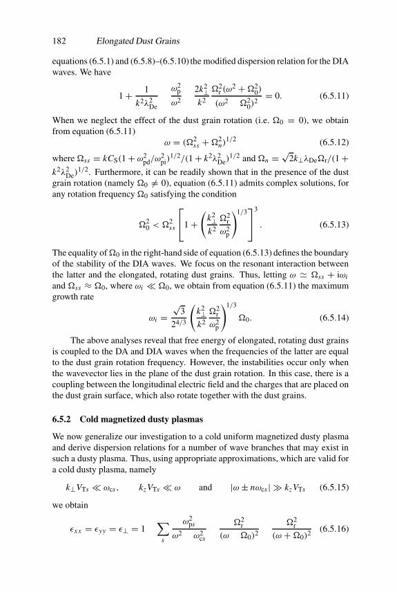
182 Elongated Dust Grains
equations (6.5.1) and (6.5.8)–(6.5.10) the modified dispersion relation for the DIAwaves. We have
1+ 1
k2λ2De
− ω2p
ω2− 2k2⊥
k2
�2r (ω
2 +�20)
(ω2 −�20)
2= 0. (6.5.11)
When we neglect the effect of the dust grain rotation (i.e. �0 = 0), we obtainfrom equation (6.5.11)
ω = (�2ss +�2
n)1/2 (6.5.12)
where �ss = kCS(1+ ω2pd/ω
2pi)
1/2/(1+ k2λ2De)
1/2 and �n =√
2k⊥λDe�r/(1+k2λ2
De)1/2. Furthermore, it can be readily shown that in the presence of the dust
grain rotation (namely �0 �= 0), equation (6.5.11) admits complex solutions, forany rotation frequency �0 satisfying the condition
�20 < �2
ss
1+
(k2⊥k2
�2r
ω2p
)1/3
3
. (6.5.13)
The equality of�0 in the right-hand side of equation (6.5.13) defines the boundaryof the stability of the DIA waves. We focus on the resonant interaction betweenthe latter and the elongated, rotating dust grains. Thus, letting ω � �ss + iωi
and �ss ≈ �0, where ωi � �0, we obtain from equation (6.5.11) the maximumgrowth rate
ωi =√
3
24/3
(k2⊥k2
�2r
ω2p
)1/3
�0. (6.5.14)
The above analyses reveal that free energy of elongated, rotating dust grainsis coupled to the DA and DIA waves when the frequencies of the latter are equalto the dust grain rotation frequency. However, the instabilities occur only whenthe wavevector lies in the plane of the dust grain rotation. In this case, there is acoupling between the longitudinal electric field and the charges that are placed onthe dust grain surface, which also rotate together with the dust grains.
6.5.2 Cold magnetized dusty plasmas
We now generalize our investigation to a cold uniform magnetized dusty plasmaand derive dispersion relations for a number of wave branches that may exist insuch a dusty plasma. Thus, using appropriate approximations, which are valid fora cold dusty plasma, namely
k⊥VTs � ωcs, kzVTs � ω and |ω ± nωcs | � kzVTs (6.5.15)
we obtain
εx x = εyy = ε⊥ = 1−∑
s
ω2ps
ω2 − ω2cs− �2
r
(ω −�0)2− �2
r
(ω +�0)2(6.5.16)
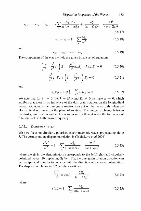
Dispersion Properties of the Waves 183
εxy = −εyx = igsr = −i∑
s
ω2psωcs
ω(ω2 − ω2cs)+ i
�2r
(ω −�0)2− i
�2r
(ω +�0)2
(6.5.17)
εzz = ε‖ = 1−∑
s
ω2ps
ω2(6.5.18)
andεxz = εzx = εyz = εzy = 0. (6.5.19)
The components of the electric field are given by the set of equations(k2
z −ω2
c2 ε⊥
)Ex − i
ω2
c2 gsrEy − k⊥kz Ez = 0 (6.5.20)
ω2
c2gsrEx +
(k2 − ω2
c2ε⊥
)Ey = 0 (6.5.21)
and
−k⊥kz Ex + (k2⊥ −ω2
c2 ε‖)Ez = 0. (6.5.22)
We note that for k⊥ = 0 (i.e. k = zkz) and Ez �= 0 we have ε‖ = 0, whichexhibits that there is no influence of the dust grain rotation on the longitudinalwaves. Obviously, the dust grain rotation can act on the waves only when theelectric field is situated in the plane of rotation. The energy exchange betweenthe dust grain rotation and such a wave is most efficient when the frequency ofrotation is close to the wave frequency.
6.5.2.1 Transverse waves
We now focus on circularly polarized electromagnetic waves propagating alongz. The corresponding dispersion relation is (Tskhakaya et al 2001)
k2z c2
ω2 = 1−∑
s
ω2ps
ω(ω ∓ ωcs)− 2�2
r
(ω ±�0)2(6.5.23)
where the ± in the denominators corresponds to the left/right-hand circularlypolarized waves. By replacing �0 by −�0, the dust grain rotation direction canbe manipulated in order to coincide with the direction of the wave polarization.The dispersion relation (6.5.23) is then written as
k2z c2
ω2= ε(ω)− 2�2
r
(ω −�0)2(6.5.24)
where
ε(ω) = 1−∑
s
ω2ps
ω(ω + ωcs). (6.5.25)

184 Elongated Dust Grains
Introducing a small frequency shift �0 around �0, we let ω = �0 + �0, where�0 � �0 and express equation (6.5.24) as
k2z c2
�20
− ε(�0)+�0∂
∂�0
[k2
z c2
�20
− ε(�0)
]= −2�2
r
�20
. (6.5.26)
If �0 is far away from the characteristic frequency ω0 of a magnetized dustyplasma, which satisfies
H (ω0) = k2z c2
ω2− ε(ω0) = 0 (6.5.27)
so that the condition
|H (�0)/�0∂H (�0)/∂�0| � �0/�0 (6.5.28)
is fulfilled (this case is referred to as a non-resonant case), we obtain
�0 = ±i√
2�r
kzc�0
[1+ �2
0
k2z c2
ε(�0)
](6.5.29)
where we have assumed that �20 � k2
z c2. Equation (6.5.29) depicts a new type ofunstable transverse wave whose frequency is close to the rotation frequency �0.In the resonance case, when the inequality in equation (6.5.28) is reversed, �0 isclose to some characteristic frequency of the magnetized dusty plasma, namely
H (�0) = 0 (6.5.30)
we obtain for the frequency shift
�0 =[− 2�2
r
�30∂H (�0)/∂�0
]1/3
�0
(1
− 1±i√
32
). (6.5.31)
Equation (6.5.31) exhibits an unstable root with a substantial growth rate, whichis proportional to �
2/3r .
We now discuss the dispersion properties of electromagnetic waves for theresonance case. As �0 is small in most of the astrophysical and terrestrialenvironments, we consider the low-frequency regimes of the plasma oscillations.For |ωcd|, ωci � ω � |ωce| we have
H (ω) = k2z c2
ω2− ω2
pe
ω|ωce| . (6.5.32)
Letting ω = �0 + iωi , where �0 � ω0 = k2z c2|ωce|/ω2
pe (the electron whistlerwaves), we obtain for the growth rate
ωi � �0
[2�2
r
k2c2
]1/3
. (6.5.33)
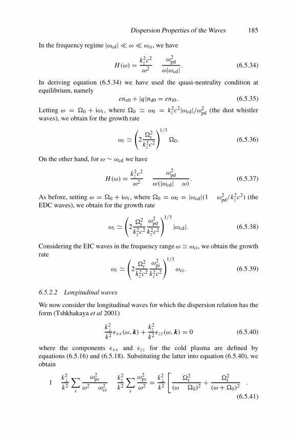
Dispersion Properties of the Waves 185
In the frequency regime |ωcd| � ω � ωci, we have
H (ω) = k2z c2
ω2− ω2
pd
ω|ωcd| . (6.5.34)
In deriving equation (6.5.34) we have used the quasi-neutrality condition atequilibrium, namely
ene0 + |q|nd0 = eni0. (6.5.35)
Letting ω = �0 + iωi , where �0 � ω0 = k2z c2|ωcd|/ω2
pd (the dust whistlerwaves), we obtain for the growth rate
ωi �(
2�2
r
k2z c2
)1/3
�0. (6.5.36)
On the other hand, for ω ∼ ωcd we have
H (ω) = k2z c2
ω2− ω2
pd
ω(|ωcd| − ω). (6.5.37)
As before, setting ω = �0 + iωi , where �0 = ω0 = |ωcd|(1 − ω2pd/k2
z c2) (theEDC waves), we obtain for the growth rate
ωi �(
2�2
r
k2z c2
ω2pd
k2z c2
)1/3
|ωcd|. (6.5.38)
Considering the EIC waves in the frequency range ω � ωci, we obtain the growthrate
ωi �(
2�2
r
k2z c2
ω2pi
k2z c2
)1/3
ωci. (6.5.39)
6.5.2.2 Longitudinal waves
We now consider the longitudinal waves for which the dispersion relation has theform (Tshkhakaya et al 2001)
k2⊥k2
εx x(ω, k) + k2z
k2εzz(ω, k) = 0 (6.5.40)
where the components εx x and εzz for the cold plasma are defined byequations (6.5.16) and (6.5.18). Substituting the latter into equation (6.5.40), weobtain
1− k2⊥k2
∑s
ω2ps
ω2 − ω2cs− k2
z
k2
∑s
ω2ps
ω2= k2⊥
k2
[�2
r
(ω −�0)2+ �2
r
(ω +�0)2
].
(6.5.41)
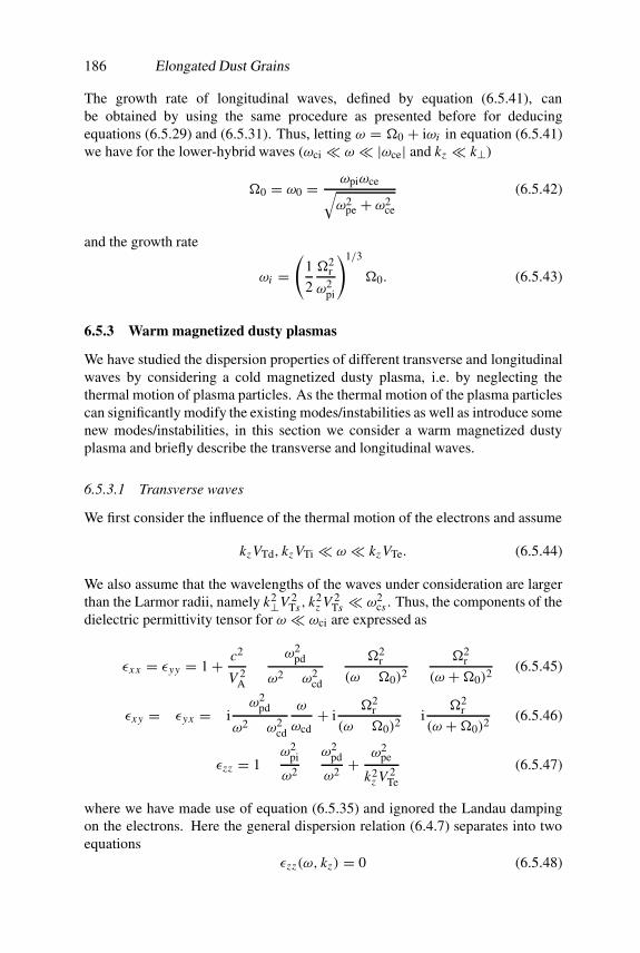
186 Elongated Dust Grains
The growth rate of longitudinal waves, defined by equation (6.5.41), canbe obtained by using the same procedure as presented before for deducingequations (6.5.29) and (6.5.31). Thus, letting ω = �0 + iωi in equation (6.5.41)we have for the lower-hybrid waves (ωci � ω � |ωce| and kz � k⊥)
�0 = ω0 = ωpiωce√ω2
pe + ω2ce
(6.5.42)
and the growth rate
ωi =(
1
2
�2r
ω2pi
)1/3
�0. (6.5.43)
6.5.3 Warm magnetized dusty plasmas
We have studied the dispersion properties of different transverse and longitudinalwaves by considering a cold magnetized dusty plasma, i.e. by neglecting thethermal motion of plasma particles. As the thermal motion of the plasma particlescan significantly modify the existing modes/instabilities as well as introduce somenew modes/instabilities, in this section we consider a warm magnetized dustyplasma and briefly describe the transverse and longitudinal waves.
6.5.3.1 Transverse waves
We first consider the influence of the thermal motion of the electrons and assume
kzVTd, kz VTi � ω � kz VTe. (6.5.44)
We also assume that the wavelengths of the waves under consideration are largerthan the Larmor radii, namely k2⊥V 2
Ts, k2z V 2
Ts � ω2cs . Thus, the components of the
dielectric permittivity tensor for ω � ωci are expressed as
εx x = εyy = 1+ c2
V 2A
− ω2pd
ω2 − ω2cd
− �2r
(ω −�0)2− �2
r
(ω +�0)2(6.5.45)
εxy = −εyx = −iω2
pd
ω2 − ω2cd
ω
ωcd+ i
�2r
(ω −�0)2− i
�2r
(ω +�0)2(6.5.46)
εzz = 1− ω2pi
ω2 −ω2
pd
ω2 +ω2
pe
k2z V 2
Te
(6.5.47)
where we have made use of equation (6.5.35) and ignored the Landau dampingon the electrons. Here the general dispersion relation (6.4.7) separates into twoequations
εzz(ω, kz) = 0 (6.5.48)
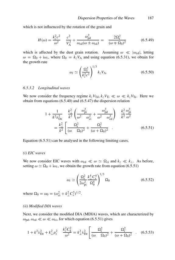
Dispersion Properties of the Waves 187
which is not influenced by the rotation of the grain and
H (ω) = k2z c2
ω2− c2
V 2A
+ ω2pd
ωcd(ω ± ωcd)= − 2�2
r
(ω ∓�0)2(6.5.49)
which is affected by the dust grain rotation. Assuming ω � |ωcd|, lettingω = �0 + iωi , where �0 = kz VA and using equation (6.5.31), we obtain forthe growth rate
ωi �(
�2r
k2z c2
)1/3
kzVA. (6.5.50)
6.5.3.2 Longitudinal waves
We now consider the frequency regime kzVTd, kz VTi � ω � kz VTe. Here weobtain from equations (6.5.40) and (6.5.47) the dispersion relation
1+ 1
k2λ2De
− k2⊥k2
(ω2
pi
ω2 − ω2ci
+ ω2pd
ω2 − ω2cd
)− k2
z
k2
ω2pi
ω2
= k2⊥k2
[�2
r
(ω −�0)2+ �2
r
(ω +�0)2
]. (6.5.51)
Equation (6.5.51) can be analysed in the following limiting cases.
(i) EIC waves
We now consider EIC waves with ωcd � ω � �ci and kz � k⊥. As before,setting ω � �0 + iωi , we obtain the growth rate from equation (6.5.51)
ωi �(
�2r
2ω2pi
k4⊥C4s
�40
)1/3
�0 (6.5.52)
where �0 = ω0 = (ω2ci + k2⊥C2
s )1/2.
(ii) Modified DIA waves
Next, we consider the modified DIA (MDIA) waves, which are characterized byωpd, ωcd � ω � ωci, for which equation (6.5.51) gives
1+ k2λ2De + k2⊥ρ2
s −k2
z C2S
ω2 = k2⊥λ2De
[�2
r
(ω −�0)2+ �2
r
(ω +�0)2
]. (6.5.53)
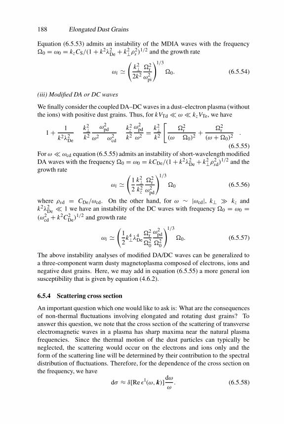
188 Elongated Dust Grains
Equation (6.5.53) admits an instability of the MDIA waves with the frequency�0 = ω0 = kzCS/(1+ k2λ2
De + k2⊥ρ2s )
1/2 and the growth rate
ωi �(
k2⊥2k2
�2r
ω2pi
)1/3
�0. (6.5.54)
(iii) Modified DA or DC waves
We finally consider the coupled DA–DC waves in a dust–electron plasma (withoutthe ions) with positive dust grains. Thus, for kVTd � ω � kzVTe, we have
1+ 1
k2λ2De
− k2⊥k2
ω2pd
ω2 − ω2cd
− k2z
k2
ω2pd
ω2 =k2⊥k2
[�2
r
(ω −�0)2+ �2
r
(ω +�0)2
].
(6.5.55)For ω � ωcd equation (6.5.55) admits an instability of short-wavelength modifiedDA waves with the frequency �0 = ω0 = kCDe/(1+ k2λ2
De + k2⊥ρ2sd)
1/2 and thegrowth rate
ωi �(
1
2
k2⊥k2
z
�2r
ω2pd
)1/3
�0 (6.5.56)
where ρsd = CDe/ωcd. On the other hand, for ω ∼ |ωcd|, k⊥ � kz andk2λ2
De � 1 we have an instability of the DC waves with frequency �0 = ω0 =(ω2
cd + k2C2De)
1/2 and growth rate
ωi �(
1
2k4⊥λ4
De�2
r
�20
ω2pd
�20
)1/3
�0. (6.5.57)
The above instability analyses of modified DA/DC waves can be generalized toa three-component warm dusty magnetoplasma composed of electrons, ions andnegative dust grains. Here, we may add in equation (6.5.55) a more general ionsusceptibility that is given by equation (4.6.2).
6.5.4 Scattering cross section
An important question which one would like to ask is: What are the consequencesof non-thermal fluctuations involving elongated and rotating dust grains? Toanswer this question, we note that the cross section of the scattering of transverseelectromagnetic waves in a plasma has sharp maxima near the natural plasmafrequencies. Since the thermal motion of the dust particles can typically beneglected, the scattering would occur on the electrons and ions only and theform of the scattering line will be determined by their contribution to the spectraldistribution of fluctuations. Therefore, for the dependence of the cross section onthe frequency, we have
dσ ≈ δ[Re εl(ω, k)]dωω. (6.5.58)

Grain Vibration and Rotation 189
The cross section, given by equation (6.5.58), has a sharp maximum at ω � �0.When the dust grain rotation frequency�0 approaches a critical value, defined byany normal mode of our dusty plasma, the fluctuations of longitudinal/transversewaves sharply increase and the scattering cross section must also sharply increase.Hence the presence of non-thermal fluctuations can be used for diagnosticpurposes. For example, coherent or incoherent scattering of star light and/orelectromagnetic waves off non-thermal fluctuations in cosmic plasmas may yieldvaluable information regarding the light polarization, the dust number densityand the dust charge in situ, as well as other plasma parameters including theexternal magnetic field strength. The existence of a preferred frequency of thedust grain rotation can also be found by means of the scattering of transverseelectromagnetic waves off enhanced low-frequency fluctuations in a dusty plasma.The usual Mie and Debye scattering theories (Guerra and Mendonca 2000) haveto be reconsidered to account for collective interactions that are dependent onelongated and rotating dust grains in plasmas.
6.6 Grain Vibration and Rotation
Studies of the levitation and dynamics of charged dust grains are of significantinterest in space and laboratory environments. Recent laboratory experiments(Rahman et al 2001) have conclusively demonstrated different types of motionsof charged dust clouds near negatively biased electrodes in low-temperature dustyplasma discharges. The dust grains in a dusty plasma sheath are levitated dueto the balance between the gravity and electrostatic forces and the dust cloudis usually located away from the electrode at a distance several times largerthan the Debye length. The dust grains execute bouncing motions which arerepeatedly away and towards the electrodes. The dust grains also performtransverse quivering across the sheath electric field. Here we discuss a theory(Tskhakaya and Shukla 2001) for the bouncing, vibrational (or quivering) androtational motions of elongated dust grains in the presence of electric fields in aplasma without and with an external magnetic field.
To describe the dynamics of a single charged dust grain in electromagneticfields, it is more convenient to start with equations (6.3.6) and (6.3.7) and separatethe motions of the centre of mass and the rotation around it. Thus, we can writevi = V +��ri and ri = r+�ri , where V and r are the velocity and positionof the centre of mass and �ri is the coordinate of the i th part of the grain relativeto the centre of mass.
The equations of motion for charged dust grains can be readily deduced fromequations (6.3.6) and (6.3.7), which are generalized to include a gravity forcemd g. We have
d pdt= (q+d ·∇)
(E + 1
cV × B
)+ 1
c(�×d)×B+(m×∇)×B+md g (6.6.1)

190 Elongated Dust Grains
and
dMα
dt= − q
2mdcIαβ
[∂Bα
∂ t+ (V · ∇)Bα
]+[
d ×(
E + 1
cV × B
)]α
+(m×B)α
(6.6.2)where p = mdV is the momentum and Mα = Iαβ�β is the angular momentumof the grain. We now consider the dust particle motions in three interesting cases.
6.6.1 Bouncing motion
We first consider a simple situation in which the effect of the magnetic field canbe neglected. Thus, the equation of motion (6.6.1) for rd/λin � 1 has the form
mddVz
dt= −∂Ub
∂z(6.6.3)
where (Tskhakaya and Shukla 2001)
Ub = qϕ + dz∂ϕ
∂z+ mdgzz (6.6.4)
is the effective potential energy and the electric field Ez = −∂ϕ/∂z is alignedalong the z-axis. The z component of the gravity is denoted by gz . Since inmost of the low-temperature laboratory dusty plasma discharges, the charge ofthe dust grains is negative, we have q < 0. For negatively biased electrodes, thepotential ϕ(< 0) tends monotonically to zero away from the electrode. In theplasma sheath, whose thickness is of the order of several Debye lengths λD, theincrease of the potential ϕ is rather sharp. Beyond this region, i.e. in the pre-sheath, the effective potential ϕ changes smoothly. Thus, between the electrodeand the unperturbed plasma, the effective potential energy Ub has the shape ofa well with a minimum at the point (z = z0) where mdgz ≈ −q∂ϕ/∂z. Hencethe grains trapped in the potential well execute bouncing motions between theelectrode and the unperturbed plasma. On the other hand, for the description ofrotational motions of dust clouds, it is necessary to account for the transverseinhomogeneity (parallel to the electrode) of the electric field.
6.6.2 Vibrational motion
We consider the quivering motion of the grains in the presence of a homogeneouselectric field E = zE , as depicted in figure 6.2. In the absence of the magneticfield, neglecting small terms that are of order rd/λin, we obtain for the angularmomentum (Tskhakaya and Shukla 2001)
dMdt
= d × E. (6.6.5)
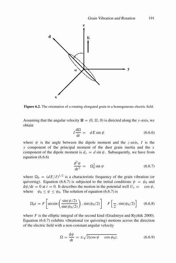
Grain Vibration and Rotation 191
Figure 6.2. The orientation of a rotating elongated grain in a homogeneous electric field.
Assuming that the angular velocity � = (0,�, 0) is directed along the y-axis, weobtain
Id�
dt= −d E sinψ (6.6.6)
where ψ is the angle between the dipole moment and the z-axis, I is they component of the principal moment of the dust grain inertia and the xcomponent of the dipole moment is dx = d sinψ . Subsequently, we have fromequation (6.6.6)
d2ψ
dt2 = −�20 sinψ (6.6.7)
where �0 = (d E/I )1/2 is a characteristic frequency of the grain vibration (orquivering). Equation (6.6.7) is subjected to the initial conditions ψ = ψ0 anddψ/dt = 0 at t = 0. It describes the motion in the potential well Uv = − cosψ ,where −ψ0 ≤ ψ ≤ ψ0. The solution of equation (6.6.7) is
�0t = F
[arcsin
(sin(ψ/2)
sin(ψ0/2)
), sin(ψ0/2)
]− F
[π2, sin(ψ0/2)
](6.6.8)
where F is the elliptic integral of the second kind (Gradsteyn and Ryzhik 2000).Equation (6.6.7) exhibits vibrational (or quivering) motions across the directionof the electric field with a non-constant angular velocity
� = dψ
dt= ±√2(cosψ − cosψ0). (6.6.9)

192 Elongated Dust Grains
It turns out that � varies in the range 0 ≤ � ≤ 2�0 sin(ψ0/2). The period of asingle swing is
T = 4√2�0
∫ ψ0
0
dψ√cosψ − cosψ0
≡ 4
�0F[π
2, sin(ψ0/2)
]. (6.6.10)
The averaged angular velocity is then 〈�〉 = (4/T )ψ0. An order of magnitudeestimate for the characteristic angular velocity for the grain quivering is
�0 ∼ 104√
14.4(Zd/mdnd)E(V cm−1). (6.6.11)
In obtaining equation (6.6.11) we have assumed that the dust grain size isapproximately 1 µm. It follows from equation (6.6.11) that the grain vibrationfrequency can reach a value of 100 kHz and more for a moderate electric fieldstrength of a few mV cm−1.
6.6.3 Rotational and vibrational motions
We consider the dust particle dynamics in the presence of a constant ambientmagnetic field B = (0, 0, B0). We assume that the dust magnetic moment isalong the direction of the ambient magnetic field and neglect the grain precision.We also consider circularly polarized electromagnetic fields and choose Ex =E cos(ωt) and Ey = E sin(ωt), where ω is the wave frequency. The x andy components of the dipole moment are dx = d cosφ and dy = d sin φ,respectively. These assumptions allow us to express equation (6.6.2) for the dustgrain rotating around the z-axis. Thus, we have (Tskhakaya and Shukla 2001)
Izd�
dt= −d E sin(φ − ωt) (6.6.12)
which can be put in the form
d2φ
dt2 = −�20z sin(φ − ωt) (6.6.13)
where �0z = (d E/Iz)1/2 and Iz is the z component of the principal moment of
the dust grain inertia. The angular velocity is now defined by � = dφ/dt . Wesolve (6.6.13) by introducing the initial conditions φ = φ0 and dφ/dt = 0, asbefore. Accordingly, integrating equation (6.6.13) we obtain
1
2�20z
(∂$
∂ t
)2
− cos$ = 1
2
ω2
�20z
− cosφ0 ≡ E (6.6.14)
where$ = φ − ωt . (6.6.15)

Grain Vibration and Rotation 193
Figure 6.3. A schematic representation of the potential Ur = − cos$ versus $.
If the effective energy E lies between −1 and 1, $ satisfies −$max < $ <
$max, as shown in figure 6.3. Here $max is defined by sin($max/2) =√sin2(φ0/2)+ ω2/4�2
0z. A typical solution of equation (6.6.14) is
�0zt = F
[arcsin
(sin(φ0/2)
sin($max/2)
), sin($max/2)
]
− F
[arcsin
(sin($/2)
sin($max/2)
), sin($max/2)
]. (6.6.16)
Equation (6.6.16) exhibits that in a system of reference rotating with the electricfield, the dust grain now vibrates (quivers) with a frequency which roughly equals�0z . The vibrational (or quivering) period is
T = 4
�0zF[π
2, sin($max/2)
]. (6.6.17)
The dust grain rotates with the frequency of the electromagnetic field and at thesame time it also vibrates (quivers) across the electric field direction. The angularvelocity is � = ω + d$/dt . It follows that the average angular velocity of thedust grain is 〈�〉 = ω, where the angular bracket denotes the averaging over thevibrational (quivering) period, given by equation (6.6.17). We note that when theeffective energy E is approximately unity, we have no quivering. When t → ∞,the angular velocity of the dust grain exactly matches the electromagnetic fieldfrequency, namely � = ω.

194 Elongated Dust Grains
For a large effective energy E , namely ω2/�20z � 1, we have again the
rotation and vibration of the dust grains. The angular velocity of such motions is
� = �20z
ω[cosφ0 − cos(ωt − φ0)] (6.6.18)
while the averaged value of � turns out to be
〈�〉 = �20z
ωcosφ0. (6.6.19)
The above model describes the trapping of elongated dust clouds in aplasma sheath that contains homogeneous and oscillating electric fields. Themodel depicts that the dust grains bounce back and forth from a negativelybiased electrode and that they also quiver simultaneously across the electric fielddirection. Physically, the present complex motions of dust clouds arise due tothe combined effects of the sheath electric field and the dipole moment of thedust grain; both of which produce a potential well that can trap and confine thedust particles. The rotation of elongated dust grains can also be set by circularlypolarized electromagnetic fields (namely helicons/whistlers or rf waves).
A charged dust particle placed in a plasma sheath may also admit spinningmotion. The sheared ion flow velocity in the sheath can induce self-rotation of aparticle, resulting in the formation of a magnetic dipole moment. The presence ofan external magnetic field can cause the spinning dust particle to precess aroundthe magnetic field direction, in addition to performing the gyro motion. Forthe laboratory dust experimental conditions (Sato et al 2000, 2001) the spinningfrequency is of the order of 10 Hz, while the precession is much slower. Ishiharaand Sato (2001) have presented a model for the dust grain spinning in the presenceof an ion flow in a magnetic field. Clearly, more experimental and rigoroustheoretical studies are needed to explore the underlying physics of rotation andspinning of elongated dust grains as well as their alignment (Mendonca et al2001), which should also play a very significant role for determining the lightpolarization in astrophysical objects.

Chapter 7
Nonlinear Structures
7.1 Introduction
We have studied in chapters 4–6 the properties of numerous waves andinstabilities by assuming a harmonic wave solution that is proportional toexp(−iωt + ik · r). This means that we have dealt with a wide variety ofsmall-amplitude waves which are driven by linear and nonlinear mechanisms.There are numerous processes via which unstable modes can saturate and attainlarge amplitudes. When the amplitudes of the waves are sufficiently large,nonlinearities cannot be ignored. The nonlinearities come from the harmonicgeneration involving fluid advection, the nonlinear Lorentz force, trapping ofparticles in the wave potential, ponderomotive force, etc. The nonlinearitiesin plasmas contribute to the localization of waves, leading to different types ofinteresting coherent structures (namely solitary structures, shock waves, vortices,etc) which are important from both theoretical and experimental points of view.
A solitary structure is a hump or dip shaped nonlinear wave of permanentprofile (to distinguish it from a soliton, we note that a soliton is a special type ofsolitary waves which preserve their shape and speed after interactions). It arisesbecause of the balance between the effects of the nonlinearity and the dispersion(when the effect of dissipation is negligible in comparison with those of thenonlinearity and dispersion). However, when the dissipative effect is comparableto or more dominant than the dispersive effect, one encounters shock waves.The small but finite amplitude solitary waves (known as the KdV solitons) aregoverned by a Korteweg–de Vries (KdV) type equation, while the shock wavesare described by a KdV–Burgers type equation. On the other hand, when theconvective derivative is in the form of a vector product (for a two-dimensionalcase), one may obtain highly nonlinear waves in the form of vortices which aregoverned by the Navier–Stokes (NS) equation (Hasegawa 1985) or the Charney–Hasegawa–Mima equation (Charney 1947, Hasegawa and Mima 1978).
The nonlinear structures, which represent the plasma states far fromthermodynamic equilibrium, are either spontaneously created in laboratory and
195

196 Nonlinear Structures
space plasmas on account of free energy sources or externally launched inlaboratory plasmas under controlled conditions. The presence of charged dustgrains introduces new features to the nonlinear structures, which are otherwiseabsent in the usual electron–ion plasma. This chapter is concerned with sometheories for numerous nonlinear structures (solitary waves, double layers, shockwaves, vortices, etc) in dusty plasmas. We also present experimental observationsof some of these nonlinear structures (e.g. DIA shocks).
7.2 Solitary Waves
To study the properties of non-envelope solitons associated with a specific wavemode, we have to account for the harmonic generation within a multi-fluiddescription and the modification of the distribution functions (due to trappedparticles) within a kinetic description. In an unmagnetized dusty plasma, we canhave solitary and shock waves (Rao et al 1990, Bharuthram and Shukla 1992a,Rao and Shukla 1994, Melandsø and Shukla 1995, Popel et al 1996, Mamun etal 1996a, Mamun 1999) as well as double layers associated with DA, DIA andDL waves. We have already shown in section 1.6 (of chapter 1) that the presenceof immobile negatively charged dust particles can modify the Bohm criterion forthe dusty plasma sheath. The modified Bohm criterion is M >
√ni0/ne0 (where
M = ion-acoustic solitary wave speed/ion-acoustic speed). This means that if wereplace the Mach number M by an effective Mach number M∗ = M/
√ni0/ne0,
the nonlinear properties of the DIA waves turn out to be the same (Bharuthramand Shukla 1992a) as those of the ion-acoustic waves in an electron–ion plasma(Sagdeev 1966, Washimi and Taniuti 1966). However, there are new features forthe DA solitary (DAS) waves (Rao et al 1990) whose dynamics is governed bythe nonlinear Boltzmann electron and ion distributions as well as the nonlineardust continuity and dust momentum equations. These are described below.
The dynamics of low phase velocity (namely VTd � Vp � VTe, VTi) one-dimensional DAS waves is governed by (Rao et al 1990)
∂nd
∂ t+ ∂
∂z(ndud) = 0 (7.2.1)
∂ud
∂ t+ ud
∂ud
∂z= ∂ϕ
∂z(7.2.2)
and∂2ϕ
∂z2= nd + µene − µini (7.2.3)
where ns is the particle number density normalized by ns0, ud is the dust fluidvelocity normalized by Cd = (Zd0kBTi/md)
1/2 and ϕ is the electrostatic wavepotential normalized by kBTi/e. The time and space variables are in units of thedust plasma period ωpd
−1 and the Debye length λDm = (kBTi/4π Zd0nd0e2)1/2,respectively. Here we have denoted µe = ne0/Zd0nd0 = 1/(δ − 1), µi =

Solitary Waves 197
ni0/Zd0nd0 = δ/(δ − 1), σi = Ti/Te and δ = ni0/ne0. The normalized electronand ion number densities are, respectively
ne = exp(σiϕ) (7.2.4)
andni = exp(−ϕ). (7.2.5)
Equations (7.2.1)–(7.2.5) are analysed for two cases. First we study small butfinite amplitude DAS waves for which we use the reductive perturbation method(Washimi and Taniuti 1966) and later we focus on arbitrary amplitude DAS wavesfor which we employ the Sagdeev potential approach (Sagdeev 1966).
7.2.1 Small-amplitude DAS waves
To study the dynamics of small but finite amplitude DAS waves, we derivethe KdV equation from equations (7.2.1)–(7.2.5) by employing the reductiveperturbation technique (Washimi and Taniuti 1966) and the stretched coordinatesζ = ε1/2(z− v0t) and τ = ε3/2t , where ε is a smallness parameter measuring theweakness of the amplitude or dispersion and v0 is the soliton speed (normalizedby Cd). We can then expand the variables nd, ud and ϕ about the unperturbedstates in power series of ε as
nd = 1+ εn(1)d + ε2n(2)d + · · · (7.2.6a)
ud = εu(1)d + ε2u(2)d + · · · (7.2.6b)
ϕ = εϕ(1) + ε2ϕ(2) + · · · (7.2.6c)
and develop equations in various powers of ε. To lowest order in ε,equations (7.2.1)–(7.2.6) give n(1)d = −ϕ(1)/v2
0 , u(1)d = −ϕ(1)/v0 and v0 =1/√µi + σiµe. To next higher order in ε, we obtain a set of equations
∂n(1)d
∂τ− v0
∂n(2)d
∂ζ+ ∂u(2)d
∂ζ+ ∂
∂ζ[n(1)d u(1)d ] = 0 (7.2.7)
∂u(1)d
∂τ− v0
∂u(2)d
∂ζ− ∂ϕ(2)
∂ζ+ u(1)d
∂u(1)d
∂ζ= 0 (7.2.8)
and∂2ϕ(1)
∂ζ 2− 1
v20
ϕ(2) − n(2)d + 1
2(µi − σ 2
i µe)[ϕ(1)]2 = 0. (7.2.9)
Combining equations (7.2.7)–(7.2.9) we readily obtain
∂ϕ(1)
∂τ+ asϕ
(1) ∂ϕ(1)
∂ζ+ bs
∂3ϕ(1)
∂ζ 3= 0 (7.2.10)
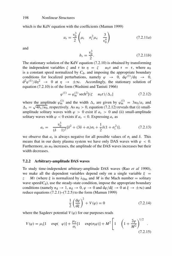
198 Nonlinear Structures
which is the KdV equation with the coefficients (Mamun 1999)
as = v30
2
(µi − σ 2
i µe − 3
v40
)(7.2.11a)
and
bs = v30
2. (7.2.11b)
The stationary solution of the KdV equation (7.2.10) is obtained by transformingthe independent variables ζ and τ to η = ζ − u0τ and τ = τ , where u0is a constant speed normalized by Cd, and imposing the appropriate boundaryconditions for localized perturbations, namely ϕ → 0, dϕ(1)/dη → 0,d2ϕ(1)/dη2 → 0 at η → ±∞. Accordingly, the stationary solution ofequation (7.2.10) is of the form (Washimi and Taniuti 1966)
ϕ(1) = ϕ(1)m sech2[(ζ − u0τ )/�s ] (7.2.12)
where the amplitude ϕ(1)m and the width �s are given by ϕ
(1)m = 3u0/as and
�s = √4bs/u0, respectively. As u0 > 0, equation (7.2.12) reveals that (i) small-amplitude solitary waves with ϕ > 0 exist if as > 0 and (ii) small-amplitudesolitary waves with ϕ < 0 exists if as < 0. Expressing as as
as = − v30
(δ − 1)2[δ2 + (3δ + σi)σi + 1
2δ(1+ σ 2
i )]. (7.2.13)
we observe that as is always negative for all possible values of σi and δ. Thismeans that in our dusty plasma system we have only DAS waves with ϕ < 0.Furthermore, as u0 increases, the amplitude of the DAS waves increases but theirwidth decreases.
7.2.2 Arbitrary-amplitude DAS waves
To study time-independent arbitrary-amplitude DAS waves (Rao et al 1990),we make all the dependent variables depend only on a single variable ξ =z − Mt (where ξ is normalized by λDm and M is the Mach number = solitarywave speed/Cd), use the steady-state condition, impose the appropriate boundaryconditions (namely nd → 1, ud → 0, ϕ → 0 and dϕ/dξ → 0 at ξ → ±∞) andreduce equations (7.2.1)–(7.2.5) to the form (Mamun 1999)
1
2
(dϕ
dξ
)2
+ V (ϕ) = 0 (7.2.14)
where the Sagdeev potential V (ϕ) for our purposes reads
V (ϕ) = µi[1− exp(−ϕ)] + µe
σi[1− exp(σiϕ)] + M2
[1−
(1+ 2ϕ
M2
)1/2].
(7.2.15)

Solitary Waves 199
It is obvious from equation (7.2.15) that V (ϕ) = dV (ϕ)/dϕ = 0 atϕ = 0. Therefore, solitary wave solutions of equation (7.2.14) exist if (i)(d2V/dϕ2)ϕ=0 < 0 so that the fixed point at the origin is unstable and (ii)(d3V/dϕ3)ϕ=0 > (<)0 for solitary waves with ϕ > (<)0. The nature of thesesolitary waves, whose amplitude tends to zero as the Mach number M tends toits critical value, can be found by expanding the Sagdeev potential V (ϕ) to thirdorder in a Taylor series in ϕ. The critical Mach number is that which correspondsto the vanishing of the quadratic term. At the same time, if the cubic term isnegative, there is a potential well on the negative side and if the cubic term ispositive, there is a potential well on the positive side. Therefore, by expandingthe Sagdeev potential V (ϕ) around the origin, the critical Mach number at whichthe second derivative changes sign can be found as
Mc =√
δ − 1
δ + σi. (7.2.16)
At this critical value of M the cubic term of V (ϕ) can be expressed as
− 1
3(δ − 1)2
[δ2 + (3δ + σi)σi + 1
2δ(1+ σ 2
i )
](7.2.17)
which reveals that the cubic term is always (for any values of σi and δ) negative,i.e. only solitary waves with ϕ < 0 can exist. In other words, arbitrary-amplitude DAS waves with ϕ > 0 are not allowed within our model. Figure 7.1depicts the variation of the critical Mach number Mc against ne0/ni0 (= 1/δ)for different values of σi. The figure shows that the critical Mach numberincreases with σi and δ. It is of interest to examine whether or not there existsan upper limit of M for which DAS waves with ϕ < 0 exist. This upperlimit of M can be found by the condition V (ϕc) ≥ 0, where ϕc = −M2/2 isthe minimum value of ϕ for which the dust number density nd is real. Thus,the upper limit of M is that maximum value of M for which Sm ≥ 0, whereSm = µi + µe/σi + M2 − µi exp(M2/2) − (µe/σi) exp(−σi M2/2). Figure 7.2shows the variation of Sm against M for different values of ne0/ni0 (= 1/δ). Wenotice that as we increase δ, the upper limit of M increases.
We have also numerically analysed the Sagdeev potential V (ϕ) and havefound the minimum and maximum values of M for which the DAS waves exist.These are incorporated in figures 7.3 and 7.4 which show that for σi = 0.05 andδ = 10, there exists a potential well only in the negative ϕ-axis, i.e. there existsolitary waves with ϕ < 0 for 0.95 < M < 1.52. The results in figure 7.1agree with those in figure 7.3, whereas the results in figure 7.2 agree with thosein figure 7.4. Theses plots also agree with our analytical results in that our dustyplasma may support only the DAS waves with ϕ < 0.

200 Nonlinear Structures
Figure 7.1. Variation of the critical Mach number Mc against ne0/ni0 for σi = 0.01 (solidcurve), σi = 0.05 (dashed curve) and σi = 0.1 (dotted curve).
7.2.3 Effect of the dust fluid temperature
The properties of the DAS waves that we have described in the preceedingsections are valid for a cold dust fluid. To include the effect of the finite dustfluid temperature (Singh and Rao 1997, Mendoza-Briceno et al 2000), we use themodified dust momentum equation
∂ud
∂ t+ ud
∂ud
∂z= ∂ϕ
∂z− σd
nd
∂Pd
∂z(7.2.18)
supplemented by the energy equation
∂Pd
∂ t+ ud
∂Pd
∂z+ 3Pd
∂ud
∂z= 0 (7.2.19)
and equations (7.2.1), (7.2.3)–(7.2.5). Here Pd is the dust fluid pressurenormalized by nd0kBTd and σd = Td/ZdTi. To obtain a solitary wave solution,we make all the dependent variables depend on a single independent variableξ = z − Mt . Thus, in the steady-state, equations (7.2.1), (7.2.18) and (7.2.3)(after substituting equations (7.2.4) and (7.2.5)) are written as
− M∂nd
∂ξ+ ∂
∂ξ(ndud) = 0 (7.2.20)
− M∂ud
∂ξ+ ud
∂ud
∂ξ+ σd
nd
∂Pd
∂ξ= ∂ϕ
∂ξ(7.2.21)
− M∂Pd
∂ξ+ ud
∂Pd
∂ξ+ 3Pd
∂ud
∂ξ= 0 (7.2.22)

Solitary Waves 201
Figure 7.2. Variation of Sm against M for σi = 0.05, ne0/ni0 = 0 (solid curve),ne0/ni0 = 0.05 (dashed curve) and ne0/ni0 = 0 (dotted curve). The upper limit of Mis that value for which Sm = 0.
and∂2ϕ
∂ξ2= nd + µe exp(σiϕ)− µi exp(−ϕ). (7.2.23)
Integrating equations (7.2.20) and (7.2.22) and imposing the appropriateboundary conditions for localized perturbations, namely ϕ→ 0, ud → 0, Pd → 1and nd → 1 at ξ →±∞, we obtain
nd = M
M − ud(7.2.24)
andPd = n3
d. (7.2.25)
If we substitute equation (7.2.24) into equation (7.2.21) and multiply the resultantequation by 2, we obtain
2M∂ud
∂ξ− 2ud
∂ud
∂ξ− 2σd
∂Pd
∂ξ+ 2
σd
Mud
∂Pd
∂ξ= −2
∂ϕ
∂ξ. (7.2.26)
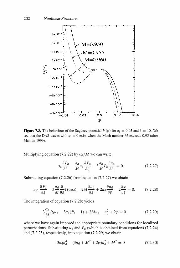
202 Nonlinear Structures
Figure 7.3. The behaviour of the Sagdeev potential V (ϕ) for σi = 0.05 and δ = 10. Wesee that the DAS waves with ϕ < 0 exist when the Mach number M exceeds 0.95 (afterMamun 1999).
Multiplying equation (7.2.22) by σd/M we can write
σd∂Pd
∂ξ− σd
Mud
∂Pd
∂ξ− 3
σd
MPd
∂ud
∂ξ= 0. (7.2.27)
Subtracting equation (7.2.26) from equation (7.2.27) we obtain
3σd∂Pd
∂ξ− 3
σd
M
∂
∂ξ(Pdud)− 2M
∂ud
∂ξ+ 2ud
∂ud
∂ξ− 2
∂ϕ
∂ξ= 0. (7.2.28)
The integration of equation (7.2.28) yields
3σd
MPdud − 3σd(Pd − 1)+ 2Mud − u2
d + 2ϕ = 0 (7.2.29)
where we have again imposed the appropriate boundary conditions for localizedperturbations. Substituting ud and Pd (which is obtained from equations (7.2.24)and (7.2.25), respectively) into equation (7.2.29) we obtain
3σdn4d − (3σd + M2 + 2ϕ)n2
d + M2 = 0 (7.2.30)
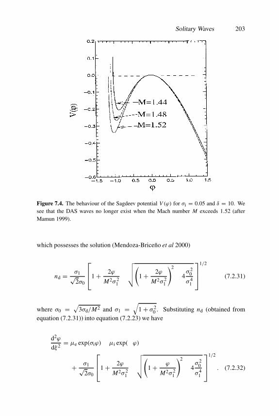
Solitary Waves 203
Figure 7.4. The behaviour of the Sagdeev potential V (ϕ) for σi = 0.05 and δ = 10. Wesee that the DAS waves no longer exist when the Mach number M exceeds 1.52 (afterMamun 1999).
which possesses the solution (Mendoza-Briceno et al 2000)
nd = σ1√2σ0
1+ 2ϕ
M2σ 21
−√√√√(1+ 2ϕ
M2σ 21
)2
− 4σ 2
0
σ 41
1/2
(7.2.31)
where σ0 =√
3σd/M2 and σ1 =√
1+ σ 20 . Substituting nd (obtained from
equation (7.2.31)) into equation (7.2.23) we have
d2ϕ
dξ2= µe exp(σiϕ)− µi exp(−ϕ)
+ σ1√2σ0
1+ 2ϕ
M2σ 21
−√√√√(1+ ϕ
M2σ 21
)2
− 4σ 2
0
σ 41
1/2
. (7.2.32)

204 Nonlinear Structures
The qualitative nature of the solutions of equation (7.2.32) is most easily seen byrewriting equation (7.2.32) in the form of an energy integral
1
2
(dϕ
dξ
)2
+ V (ϕ, M, σd, σi, δ) = 0 (7.2.33)
where the Sagdeev potential V (ϕ, M, σd, σi, δ) is
V (ϕ, M, σd, σi, δ) = −(µe
σi
)exp(σiϕ)− µi exp(−ϕ)
− M2√σ0[eθ/2 + 13 e−3θ/2] + C1 (7.2.34)
with
θ = cosh−1
[σ 2
1
2σ0
(1+ 2ϕ
M2σ 21
)](7.2.35)
and C1 is an integration constant which we choose such that V (ϕ, M, σd, σi, δ) =0 at ϕ = 0. It is important to note here that we cannot consider the limit σd → 0in the Sagdeev potential V (ϕ, M, σd, σi, δ) in its present form. To consider thelimit σd → 0, we express θ as
θ = ln
σ 2
1
2σ0
(1+ 2ϕ
M2σ 21
)+√√√√ σ 4
1
4σ 20
(1+ 2ϕ
M2σ 21
)2
− 1
. (7.2.36)
We note that in our study the condition for the ion density to be real requires|1+ 2ϕ/M2σ 2
1 | ≥ 2σ0/σ21 .
One can now examine how the dust fluid temperature σd modifies theproperties of arbitrary-amplitude DAS waves by analysing the Sagdeev potentialV (ϕ, M, σd, σi, δ), as we described in the previous section. We can also examinethe effect of the dust fluid temperature on the DAS waves by direct numericalsolitary wave solutions of equation (7.2.33) for different values of σd, as shownin figure 7.5. It is obvious from figure 7.5 that as we increase the dust fluidtemperature, the amplitude of the solitary wave decreases, but the width increases.
7.2.4 Effect of the trapped ion distribution
It is well known (Schamel 1972, 1986) that the electron and ion distributionfunctions can be significantly modified in the presence of large-amplitude wavesthat are excited by the two-stream instability (Winske et al 1995). Accordingly,the electron and ion number densities depart from the Boltzmann distributionswhen phase space vortex distributions appear in a plasma. For the DA waves,the ion trapping in the wave potential is of interest. To study the effects of

Solitary Waves 205
Figure 7.5. Potential profiles for σi = 0.2, δ = 10, M = 1.455 and σd = 0 (solid curve),σd = 0.02 (dotted curve) and σd = 0.03 (dashed curve).
non-isothermal ions on the DAS waves, we consider the trapped or vortex-like(Schamel 1972, Schamel et al 2001) ion distribution fi = fif + fit, where
fif = 1√2π
exp
[−1
2(v2
i + 2ϕ)
](7.2.37)
for |vi| > √−2ϕ and
fit = 1√2π
exp
[−1
2σit(v
2i + 2ϕ)
](7.2.38)
for |vi| ≤ √−2ϕ. We note that the ion distribution function, as prescribedabove, is continuous in velocity space and satisfies the regularity requirementsfor an admissible BGK solution (Schamel 1972). Here the ion velocity vi inequations (7.2.37) and (7.2.38) is normalized by the ion thermal velocity VTi andσit (= Ti/Tit), which is the ratio of the free ion temperature Ti to the trappedion temperature Tit, is a parameter determining the number of trapped ions.Integrating the ion distributions over the velocity space we readily obtain the ionnumber density ni as (Schamel 1986)
ni = I (−ϕ)+ 1√σit
exp(−σitϕ) erf(√−σitϕ) (7.2.39)
for σit > 0 and
ni = I (−ϕ)+ 1√π |σit|WD(
√σitϕ) (7.2.40)
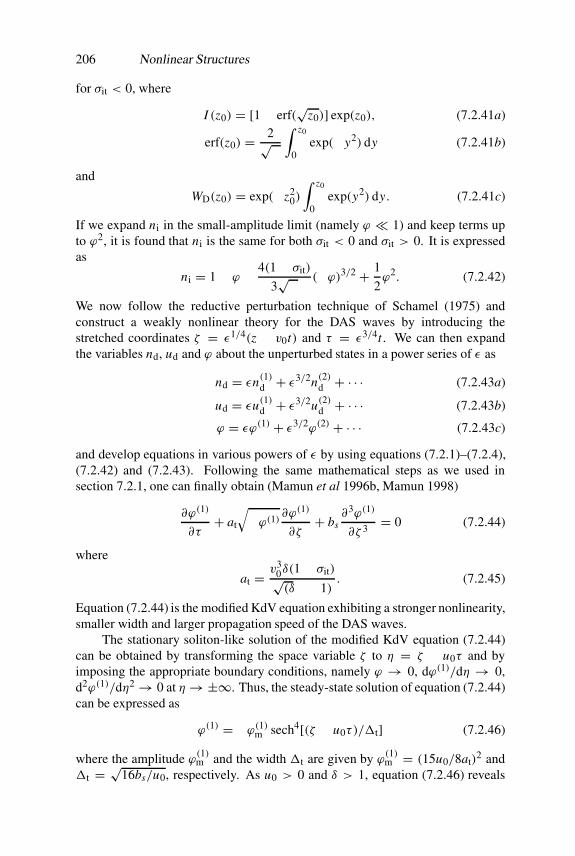
206 Nonlinear Structures
for σit < 0, where
I (z0) = [1− erf(√
z0)] exp(z0), (7.2.41a)
erf(z0) = 2√π
∫ z0
0exp(−y2) dy (7.2.41b)
and
WD(z0) = exp(−z20)
∫ z0
0exp(y2) dy. (7.2.41c)
If we expand ni in the small-amplitude limit (namely ϕ � 1) and keep terms upto ϕ2, it is found that ni is the same for both σit < 0 and σit > 0. It is expressedas
ni = 1− ϕ − 4(1− σit)
3√π
(−ϕ)3/2 + 1
2ϕ2. (7.2.42)
We now follow the reductive perturbation technique of Schamel (1975) andconstruct a weakly nonlinear theory for the DAS waves by introducing thestretched coordinates ζ = ε1/4(z − v0t) and τ = ε3/4t . We can then expandthe variables nd, ud and ϕ about the unperturbed states in a power series of ε as
nd = εn(1)d + ε3/2n(2)d + · · · (7.2.43a)
ud = εu(1)d + ε3/2u(2)d + · · · (7.2.43b)
ϕ = εϕ(1) + ε3/2ϕ(2) + · · · (7.2.43c)
and develop equations in various powers of ε by using equations (7.2.1)–(7.2.4),(7.2.42) and (7.2.43). Following the same mathematical steps as we used insection 7.2.1, one can finally obtain (Mamun et al 1996b, Mamun 1998)
∂ϕ(1)
∂τ+ at
√−ϕ(1) ∂ϕ
(1)
∂ζ+ bs
∂3ϕ(1)
∂ζ 3= 0 (7.2.44)
where
at = v30δ(1− σit)√π(δ − 1)
. (7.2.45)
Equation (7.2.44) is the modified KdV equation exhibiting a stronger nonlinearity,smaller width and larger propagation speed of the DAS waves.
The stationary soliton-like solution of the modified KdV equation (7.2.44)can be obtained by transforming the space variable ζ to η = ζ − u0τ and byimposing the appropriate boundary conditions, namely ϕ → 0, dϕ(1)/dη → 0,d2ϕ(1)/dη2 → 0 at η→±∞. Thus, the steady-state solution of equation (7.2.44)can be expressed as
ϕ(1) = −ϕ(1)m sech4[(ζ − u0τ )/�t] (7.2.46)
where the amplitude ϕ(1)m and the width �t are given by ϕ(1)m = (15u0/8at)
2 and�t = √16bs/u0, respectively. As u0 > 0 and δ > 1, equation (7.2.46) reveals
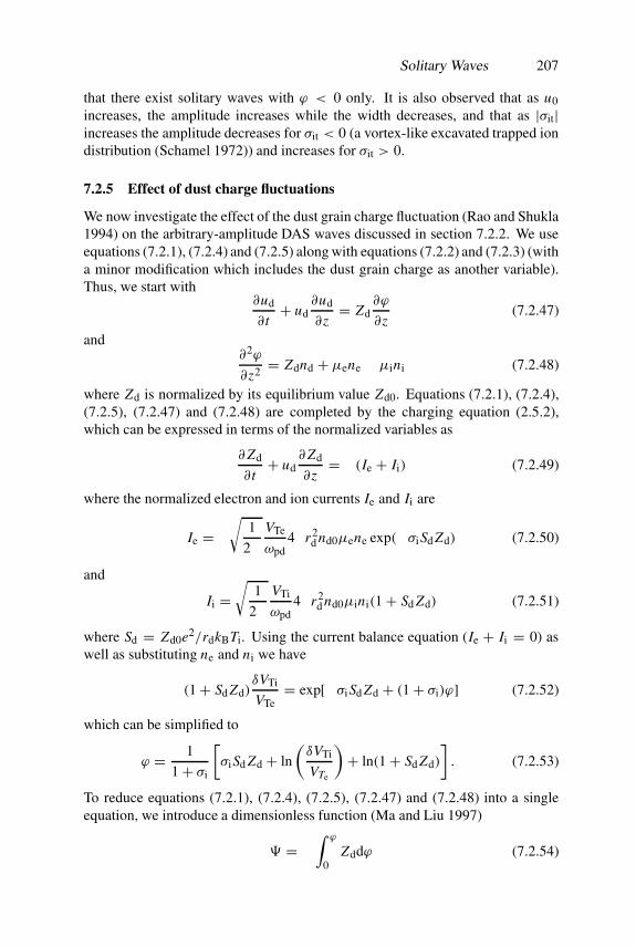
Solitary Waves 207
that there exist solitary waves with ϕ < 0 only. It is also observed that as u0increases, the amplitude increases while the width decreases, and that as |σit|increases the amplitude decreases for σit < 0 (a vortex-like excavated trapped iondistribution (Schamel 1972)) and increases for σit > 0.
7.2.5 Effect of dust charge fluctuations
We now investigate the effect of the dust grain charge fluctuation (Rao and Shukla1994) on the arbitrary-amplitude DAS waves discussed in section 7.2.2. We useequations (7.2.1), (7.2.4) and (7.2.5) along with equations (7.2.2) and (7.2.3) (witha minor modification which includes the dust grain charge as another variable).Thus, we start with
∂ud
∂ t+ ud
∂ud
∂z= Zd
∂ϕ
∂z(7.2.47)
and∂2ϕ
∂z2 = Zdnd + µene − µini (7.2.48)
where Zd is normalized by its equilibrium value Zd0. Equations (7.2.1), (7.2.4),(7.2.5), (7.2.47) and (7.2.48) are completed by the charging equation (2.5.2),which can be expressed in terms of the normalized variables as
∂Zd
∂ t+ ud
∂Zd
∂z= −(Ie + Ii) (7.2.49)
where the normalized electron and ion currents Ie and Ii are
Ie = −√
1
2π
VTe
ωpd4πr2
d nd0µene exp(−σiSd Zd) (7.2.50)
and
Ii =√
1
2π
VTi
ωpd4πr2
d nd0µini(1+ Sd Zd) (7.2.51)
where Sd = Zd0e2/rdkBTi. Using the current balance equation (Ie + Ii = 0) aswell as substituting ne and ni we have
(1+ Sd Zd)δVTi
VTe= exp[−σiSd Zd + (1+ σi)ϕ] (7.2.52)
which can be simplified to
ϕ = 1
1+ σi
[σiSd Zd + ln
(δVTi
VTe
)+ ln(1+ Sd Zd)
]. (7.2.53)
To reduce equations (7.2.1), (7.2.4), (7.2.5), (7.2.47) and (7.2.48) into a singleequation, we introduce a dimensionless function (Ma and Liu 1997)
# = −∫ ϕ
0Zddϕ (7.2.54)

208 Nonlinear Structures
which, after using equation (7.2.53), can be expressed as
# = − ϕ
Sd− (Zd − 1)− σiSd
2(1+ σi)(Z2
d − 1). (7.2.55)
To study arbitrary amplitude time-independent DAS waves, we make all thedependent variables depend only on a single variable ξ = z−Mt , use the steady-state condition and impose the appropriate boundary conditions for localizedperturbations. Hence from equations (7.2.1), (7.2.47) and (7.2.54) we obtain
nd =(
1− 2#
M2
)−1/2
. (7.2.56)
Substituting equations (7.2.4), (7.2.5) and (7.2.56) into equation (7.2.48) andintegrating the resultant equation we obtain the ‘energy integral’
1
2
(dϕ
dξ
)2
+ V (ϕ, Zd) = 0 (7.2.57)
where the Sagdeev potential V (ϕ, Zd) is of the form
V (ϕ, Zd) = µi[1− exp(−ϕ)] + µe
σi[1− exp(σiϕ)] + M2
[(1− 2#
M2
)1/2
− 1
].
(7.2.58)It is obvious from equation (7.2.58) that the effect of dust grain charge fluctuationsis contained in # . Now analysing the Sagdeev potential V (ϕ, Zd) (as wehave done in section 7.2.2), one can easily investigate the properties of theDAS waves accounting for dust charge fluctuations. We can also directly solveequation (7.2.57) numerically and examine the structures of the DAS profiles (asshown in figure 7.6) that may exist in a dusty plasma with fluctuating charges onthe dust grain surface.
7.2.6 Cylindrical and spherical DAS waves
The studies of the DAS waves that we have presented up to now are restrictedto a planar one-dimensional geometry. However, in laboratory devices one mayencounter multi-dimensional DAS structures. Here we are concerned with thepropagation of radially ingoing DAS structures in non-planar cylindrical andspherical geometries. The dynamics of low phase velocity nonlinear DAS wavesin cylindrical and spherical geometries are governed by
∂nd
∂ t+ 1
rν∂
∂r(rνndud) = 0 (7.2.59)
∂ud
∂ t+ ud
∂ud
∂r= ∂ϕ
∂r(7.2.60)
1
rν∂
∂r
(rν∂ϕ
∂r
)= nd + µe exp(σiϕ)− µi exp(−ϕ) (7.2.61)

Solitary Waves 209
Figure 7.6. Solitary wave solutions of equation (7.2.57) with σi = 1 and M = S−1/2d :
(a) potential profiles for δ = 3 and δ = 1.5, and (b) electron, ion and dust density profilesfor δ = 3 (after Ma and Liu 1997).
where ν = 1, 2 for cylindrical and spherical geometries, respectively. The spacevariable r is normalized by the Debye radius λDm.
To investigate ingoing solutions of equations (7.2.59)–(7.2.61), we introducethe stretched coordinates ζ = −ε1/2(r+v0t) and τ = ε3/2t and use the expansionof nd, ud and ϕ, as given in equation (7.2.6). Following the same procedure asapplied in section 7.2.1, we can readily derive
∂ϕ(1)
∂τ+ ν
2τϕ(1) + asϕ
(1) ∂ϕ(1)
∂ζ+ bs
∂3ϕ(1)
∂ζ 3= 0 (7.2.62)
which is a modified KdV equation with the coefficients as and bs given byequation (7.2.11). It is obvious that in equation (7.2.62) the second term, namely(ν/2τ )ϕ(1), is due to the effect of the cylindrical or spherical geometry (Maxonand Viecelli 1974). One can numerically solve equation (7.2.62) by using a two-level finite difference approximation method (Maxon and Viecelli 1974) and canstudy the effects of cylindrical and spherical geometries on time-dependent DASwaves.
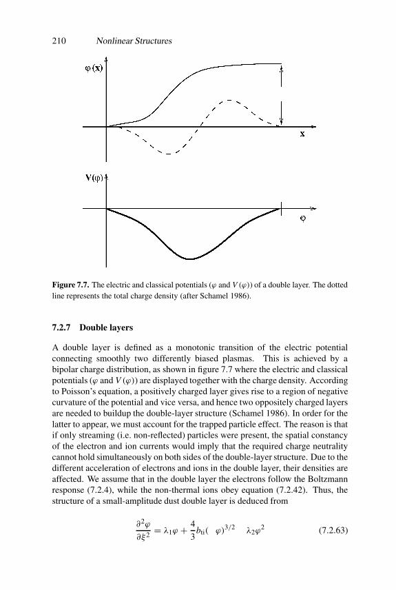
210 Nonlinear Structures
Figure 7.7. The electric and classical potentials (ϕ and V (ϕ)) of a double layer. The dottedline represents the total charge density (after Schamel 1986).
7.2.7 Double layers
A double layer is defined as a monotonic transition of the electric potentialconnecting smoothly two differently biased plasmas. This is achieved by abipolar charge distribution, as shown in figure 7.7 where the electric and classicalpotentials (ϕ and V (ϕ)) are displayed together with the charge density. Accordingto Poisson’s equation, a positively charged layer gives rise to a region of negativecurvature of the potential and vice versa, and hence two oppositely charged layersare needed to buildup the double-layer structure (Schamel 1986). In order for thelatter to appear, we must account for the trapped particle effect. The reason is thatif only streaming (i.e. non-reflected) particles were present, the spatial constancyof the electron and ion currents would imply that the required charge neutralitycannot hold simultaneously on both sides of the double-layer structure. Due to thedifferent acceleration of electrons and ions in the double layer, their densities areaffected. We assume that in the double layer the electrons follow the Boltzmannresponse (7.2.4), while the non-thermal ions obey equation (7.2.42). Thus, thestructure of a small-amplitude dust double layer is deduced from
∂2ϕ
∂ξ2= λ1ϕ + 4
3bti(−ϕ)3/2 − λ2ϕ
2 (7.2.63)
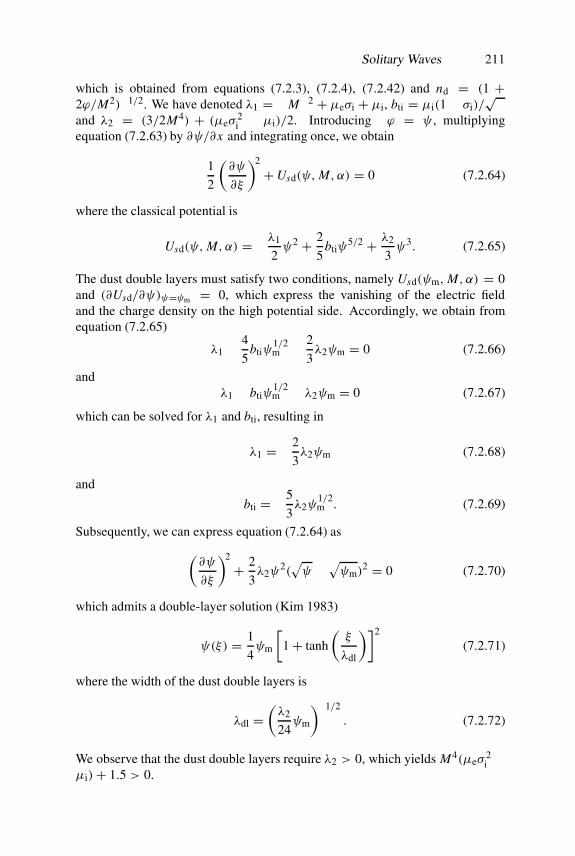
Solitary Waves 211
which is obtained from equations (7.2.3), (7.2.4), (7.2.42) and nd = (1 +2ϕ/M2)−1/2. We have denoted λ1 = −M−2 + µeσi + µi, bti = µi(1 − σi)/
√π
and λ2 = (3/2M4) + (µeσ2i − µi)/2. Introducing −ϕ = ψ , multiplying
equation (7.2.63) by ∂ψ/∂x and integrating once, we obtain
1
2
(∂ψ
∂ξ
)2
+Usd(ψ, M, α) = 0 (7.2.64)
where the classical potential is
Usd(ψ, M, α) = −λ1
2ψ2 + 2
5btiψ
5/2 + λ2
3ψ3. (7.2.65)
The dust double layers must satisfy two conditions, namely Usd(ψm, M, α) = 0and (∂Usd/∂ψ)ψ=ψm = 0, which express the vanishing of the electric fieldand the charge density on the high potential side. Accordingly, we obtain fromequation (7.2.65)
λ1 − 4
5btiψ
1/2m − 2
3λ2ψm = 0 (7.2.66)
andλ1 − btiψ
1/2m − λ2ψm = 0 (7.2.67)
which can be solved for λ1 and bti, resulting in
λ1 = −2
3λ2ψm (7.2.68)
and
bti = −5
3λ2ψ
1/2m . (7.2.69)
Subsequently, we can express equation (7.2.64) as
(∂ψ
∂ξ
)2
+ 2
3λ2ψ
2(√ψ −√ψm)
2 = 0 (7.2.70)
which admits a double-layer solution (Kim 1983)
ψ(ξ) = 1
4ψm
[1+ tanh
(ξ
λdl
)]2
(7.2.71)
where the width of the dust double layers is
λdl =(λ2
24ψm
)−1/2
. (7.2.72)
We observe that the dust double layers require λ2 > 0, which yields M4(µeσ2i −
µi)+ 1.5 > 0.

212 Nonlinear Structures
7.2.8 Dust lattice solitary waves
The linear propagation of the dust lattice waves has been studied in section 4.5.We consider here the nonlinear propagation of small but finite amplitudeDL waves for which we can express the potential energy u (given byequation (4.5.19)) in the form (Farokhi et al 1999)
u = Q0$0
cosh(kDa)
[1+ k2
D4 (ξn+1 + ξn−1 − 2ξn)
2 + k4D
384(ξn+1 + ξn−1 − 2ξn)4]
[1+ kD
2 tanh(kDa)(ξn+1 − ξn−1)] .
(7.2.73)Using equation (7.2.73) the nonlinear equation (4.5.2) can be written as
∂2ξn
∂ t2= Q0$0k2
D
md cosh(kDa)
[(ξn+1 + ξn−1 − 2ξn)+ k2
D48 (ξn+1 + ξn−1 − 2ξn)
3]
[1+ kD
2 tanh(kDa)(ξn+1 − ξn−1)]
(7.2.74)where dust–neutral collisions have been neglected. To simplify the nonlinearequation (7.2.74), we only include weak nonlinearities. We also consider thelong-wavelength approximation (kDa � 1), where the wave dispersion is smalland equation (7.2.74) can be approximated by the differential equations for acontinuum. Thus, we introduce the Taylor expansions of ξn+1 and ξn−1 as ξn +(∂ξ/∂z)na+0.5(∂2ξ/∂z2)na2+· · · and ξn−(∂ξ/∂z)na+0.5(∂2ξ/∂z2)na2+· · ·,respectively. Inserting these expansions in equation (7.2.74), we obtain (Farokhiet al 1999)
∂2ξ
∂ t2− v2
0
[∂2ξ
∂z2+ a2
12
∂4ξ
∂z4− kDa
2tanh(kDa)
∂
∂z
(∂ξ
∂z
)2]= 0. (7.2.75)
Here
v0 =[
Q0$0k2Da2
md cosh(kDa)
]1/2
(7.2.76)
is the phase velocity for kDa � 1, where the Debye shielding around eachdust particle has been neglected. Equation (7.2.75) includes the DL wavespropagating in both positive and negative z directions with phase velocities closeto v0 and −v0, respectively. For the waves with phase velocities close to v0,equation (7.2.75) takes the form
(∂
∂ t+ v0
∂
∂z
)ξ + v0
[a2
12
∂3ξ
∂z3 −kDa
2tanh(kDa)
(∂ξ
∂z
)2]= 0. (7.2.77)
Equation (7.2.77) is now transformed to a wave-frame moving with a relativespeed v0 in a new frame (z′ = z − v0t and τ = t). It is then differentiated with
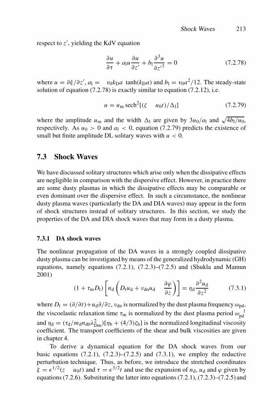
Shock Waves 213
respect to z′, yielding the KdV equation
∂u
∂τ+ alu
∂u
∂z′+ bl
∂3u
∂z′3= 0 (7.2.78)
where u = ∂ξ/∂z′, al = −v0kDa tanh(kDa) and bl = v0a2/12. The steady-statesolution of equation (7.2.78) is exactly similar to equation (7.2.12), i.e.
u = um sech2[(ζ − u0t)/�l] (7.2.79)
where the amplitude um and the width �l are given by 3u0/al and√
4bl/u0,respectively. As u0 > 0 and al < 0, equation (7.2.79) predicts the existence ofsmall but finite amplitude DL solitary waves with u < 0.
7.3 Shock Waves
We have discussed solitary structures which arise only when the dissipative effectsare negligible in comparison with the dispersive effect. However, in practice thereare some dusty plasmas in which the dissipative effects may be comparable oreven dominant over the dispersive effect. In such a circumstance, the nonlineardusty plasma waves (particularly the DA and DIA waves) may appear in the formof shock structures instead of solitary structures. In this section, we study theproperties of the DA and DIA shock waves that may form in a dusty plasma.
7.3.1 DA shock waves
The nonlinear propagation of the DA waves in a strongly coupled dissipativedusty plasma can be investigated by means of the generalized hydrodynamic (GH)equations, namely equations (7.2.1), (7.2.3)–(7.2.5) and (Shukla and Mamun2001)
(1+ τm Dt)
[nd
(Dtud + νdnud − ∂ϕ
∂z
)]= ηd
∂2ud
∂z2(7.3.1)
where Dt = (∂/∂ t)+ud∂/∂z, νdn is normalized by the dust plasma frequencyωpd,the viscoelastic relaxation time τm is normalized by the dust plasma period ω−1
pd
and ηd = (τd/mdnd0λ2Dm)[ηb + (4/3)ζb] is the normalized longitudinal viscosity
coefficient. The transport coefficients of the shear and bulk viscosities are givenin chapter 4.
To derive a dynamical equation for the DA shock waves from ourbasic equations (7.2.1), (7.2.3)–(7.2.5) and (7.3.1), we employ the reductiveperturbation technique. Thus, as before, we introduce the stretched coordinatesξ = ε1/2(z − u0t) and τ = ε3/2t and use the expansion of nd, ud and ϕ given byequations (7.2.6). Substituting the latter into equations (7.2.1), (7.2.3)–(7.2.5) and

214 Nonlinear Structures
(7.3.1), we obtain from the equations of the lowest order in ε, u(1)d = −ϕ(1)/v0,
n(1)d = −ϕ(1)/v20 and v0 = (σiµe + µi)
−1/2. To next order in ε, we have
∂n(1)d
∂τ− v0
∂n(2)d
∂ξ+ ∂
∂ξ[n(1)d u(1)d ] +
∂u(2)d
∂ξ= 0 (7.3.2)
(1+ νdnτm)∂u(1)d
∂τ− u0
∂u(2)d
∂ξ− ∂ϕ(2)
∂ξ+ (1− νdnτm)u
(1)d
∂u(1)d
∂ξ− ηd0
∂2u(1)d
∂ξ2= 0
(7.3.3)
and∂2ϕ(1)
∂ξ2− 1
u20
ϕ(2) − n(2)d = 1
2(σ 2
i µe − µi)[ϕ(1)]2 (7.3.4)
where we have assumed ηd ∼ ε1/2ηd0. By eliminating n(2)d , u(2)d and ϕ(2) fromequations (7.3.2)–(7.3.4) we readily obtain the KdV–Burgers equation
A−1d
∂ϕ(1)
∂τ+ ϕ(1)
∂ϕ(1)
∂ξ+ βd
∂3ϕ(1)
∂ξ3= µda
∂2ϕ(1)
∂ξ2(7.3.5)
where Ad = (v30ad/2)(1 + νdnτm/2)−1, µda = ηd0/adv
30 , βd = 1/ad and ad =
[(νdnτm − 3)/v40 + µi − µeσ
2i ]. As νdn > 0, τm > 0, ηd0 > 0, and v0 = (σiµe +
µi)−1/2 > 0, the sign of the coefficients Ad, βd and µda are determined by the
sign of ad, which can be expressed as ad = (νdnτm−3)(µi+σiµe)2−σ 2
i µe+µi =µe[(νdnτm−3)σ 2
i µe−σ 2i ]+µ2
i (νdnτm−3+ Zdnd0/ni0)+2(νdnτm−3)µeµiσi. Itis obvious that for a strongly coupled dusty plasma with a significant backgroundof neutrals, we have νdnτm � 1, i.e. ad > 0, which corresponds to Ad > 0,µda > 0 and βd > 0, whereas for a weakly coupled or a collisionless dustyplasma (νdnτm → 0), we have ad < 0, which corresponds to Ad < 0, µda < 0and βd < 0.
7.3.2 DIA shock waves
We present here an analytical model for the one-dimensional DIA shocks in anunmagnetized dusty plasma. The governing nonlinear equations for the DIAshocks in terms of normalized variables are (Shukla 2000d)
∂ni
∂ t+ ∂(niui)
∂z= 0 (7.3.6)
∂ui
∂ t+ ui
∂ui
∂z= −∂$
∂z− 3σini
∂ni
∂z+ ηi
∂2ui
∂z2(7.3.7)
and
δ∂2$
∂z2= exp($)− δni + (δ − 1) (7.3.8)

Shock Waves 215
where ui is the ion fluid speed normalized by the ion-acoustic speed cs , $ isthe electrostatic wave potential normalized by kBTe/e and ηi = δµd/ωpiλ
2De (in
which µd is the kinematic viscosity). Here the time and space variables are inunits of the ion plasma period ωpi
−1 and the electron Debye length λDe/√δ,
respectively.To derive a dynamical equation for the DIA shock waves, we expand
ni = 1+ εn(1)i + ε2n(2)i + · · · (7.3.9a)
ui = εu(1)i + ε2u(2)i + · · · (7.3.9b)
and$ = ε$(1) + ε2$(2) + · · · (7.3.9c)
and introduce the stretched variables ξ = ε1/2(z − v0t) and τ = ε3/2t . Nowsubstituting equations (7.3.9) into (7.3.6)–(7.3.8), we obtain from the lowest orderin ε, $(1) = δn(1)i , u(1)i = v0n(1)i and v0 = (δ + 3σi)
1/2. To next order in ε, wehave
∂n(1)i
∂τ− v0
∂n(2)i
∂ξ+ ∂
∂ξ[n(1)i u(1)i ] +
∂u(2)i
∂ξ= 0 (7.3.10)
∂u(1)i
∂τ− v0
∂u(2)i
∂ξ+ u(1)i
∂u(1)i
∂ξ
= −∂$(2)
∂ξ+ ηi0
∂2u(1)i
∂ξ2 − 3σin(1)i
∂n(1)i
∂ξ− 3σi
∂n(2)i
∂ξ(7.3.11)
and
δ∂2$(1)
∂ξ2= 1
2[$(1)]2 +$(2) − n(2)i δ (7.3.12)
where we have assumed ηi = ε1/2ηi0. Eliminating n(2)i , u(2)i and $(2) from(7.3.10)–(7.3.12) we readily obtain the desired KdV–Burgers equation
A−1i
∂$(1)
∂τ+$(1) ∂$
(1)
∂ξ+ βi
∂3$(1)
∂ξ3− µi
∂2$(1)
∂ξ2= 0 (7.3.13)
where Ai = ai/2v0, βi = δ2/ai, µi = v0ηi0/ai and ai = (3δ − δ2 + 12σi)/δ. Asv0 > 0 and ηi0 > 0, the sign of the coefficients Ai, βi and µi are determined bythe sign of ai.
7.3.3 Solutions of the KdV–Burgers equation
We now discuss possible stationary solutions of the KdV–Burgers equation (7.3.5)or (7.3.13) which can be written in the form
A−1 ∂y
∂τ+ y
∂y
∂ξ+ β
∂3y
∂ξ3= µ
∂2y
∂ξ2(7.3.14)
216 Nonlinear Structures
where y = $(1) for the DIA shock waves, while y = φ(1) for the DA shockwaves. We first transform the space variables ξ to ζ = ξ − U0τ , where U0 is thenormalized velocity of the shock waves and find a third-order ordinary differentialequation for y(ζ ). The latter can be integrated once, yielding
βδ2y
∂ζ 2 − µ∂y
∂ζ+ 1
2y2 − U0
Ay = 0 (7.3.15)
where we have imposed the appropriate boundary conditions, namely y → 0,dy/dζ → 0, d2y/dζ 2 → 0 at ζ →∞. We can now easily show (Karpman 1975,Hasegawa 1975) that equation (7.3.15) describes a shock wave whose velocity(in the reference frame under consideration) U0 is related to the extreme valuesy(−∞) − y(∞) = Y by U0/A = Y/2. Thus, in the rest frame the normalizedvelocity of the shock waves is (1+AY/2). The nature of the structure of the shockwaves depends on the relation between the dispersive and dissipative parametersβ and µ.
We first consider a situation where the dissipative term is dominant over thedispersive term. In this case, we can express equation (7.3.15) as
(y − U0
A
)dy
dζ= µ
d2y
dζ 2. (7.3.16)
Equation (7.3.16) can be easily integrated, using the condition that y is boundedas ζ →±∞, to obtain (Karpman 1975)
y = U0
A
[1− tanh
(U0
2Aµ(ξ −U0τ )
)]. (7.3.17)
Equation (7.3.17) represents a monotonic shock solution with the shock speed,the shock height and the shock thickness given by U0, U0/A and Aµ/U0,respectively. The shock solution appears because of the dissipative term, which isproportional to the viscosity coefficient.
We now discuss the effects of the dispersive term on the shock solutionof equation (7.3.15). When µ is extremely small, the shock wave will have anoscillatory profile in which the first few oscillations at the wave front will beclose to solitons (Karpman 1975) moving with velocity U0. If µ is increasedand it is larger than a certain critical value µc, the shock wave will have amonotonic behaviour. To determine the values of the dissipation coefficientµ corresponding to monotonic or oscillating shock profiles, we investigate theasymptotic behaviour of the solutions of equation (7.3.15) for ζ →−∞. We firstsubstitute y(ζ ) = y0 + y1(ζ ), where y1 � y0, into equation (7.3.15) and thenlinearize it with respect to y1 in order to obtain
βδ2y1
∂ζ 2− µ
∂y1
∂ζ+ U0
Ay1 = 0. (7.3.18)

Shock Waves 217
The solutions of equation (7.3.18) are proportional to exp(ps x), where ps is givenby
ps = µ
2β±(µ2
4β2− U0
Aβ
)1/2
. (7.3.19)
It turns out that the shock wave has a monotonic profile for µ > µc and anoscillatory profile for µ < µc, where µc = (4βU0/A)1/2. Thus, for µ < µc, thestationary solution of equation (7.3.14) is (Karpman 1975)
y = y0 + C exp
(ζ ′µ2β
)cos
(ζ ′√
U0
Aβ
)(7.3.20)
where ζ ′ = ζ −U0τ and C is a constant.
7.3.4 Experimental observations of DIA shock waves
Recently the DIA shock waves were experimentally excited in a dusty doubleplasma (DP) device by Nakamura et al (1999). Here we briefly illustrate theformation of these experimentally excited DIA shock waves by summarizing theexperimental work of Nakamura et al (1999). The inner diameter of the dusty DPdevice is 40 cm and its length is 90 cm. The device is separated into a sourceand a target section by a fine mesh grid which is kept electrically floating. Thechamber is evacuated down to 5 × 10⁻⁷ Torr with a turbo-molecular pump. Theargon gas is bled into the chamber at a partial pressure of about 5 × 10⁻⁴ Torr.A dust dispersing set-up fitted at the target section consisted of a dust reservoircoupled to an ultrasonic vibrator. The dust reservoir consists of a fine stainlesssteel mesh (118 lines per cm) of 10 cm (width) ×16 cm (axial length) area atthe bottom end and is placed horizontally closer to the anode wall. An ultrasonicvibrator is tuned at 27 kHz to vibrate the dust reservoir by using a signal generatorand a power amplifier. Glass powder of average diameter 8.8 µm is used. Thedust number density is easily controlled by adjusting the power of the signalapplied to the vibrator and is measured from the extinction intensity of the laserlight which passes through the dust column and is collected by a photodiodearray. A maximum dust density of the order of 105 cm−3 is obtained in thisset-up. The plasma parameters measured by a plane Langmuir probe of 6 mmdiameter and a retarding potential analyser are as follows: ne = 108–109 cm−3,Te = (1–1.5)× 104 K, Ti � 0.1Te, Zd � 105 for nd < 103 cm−3 and Zd � 102
for nd < 105 cm−3.The shock waves are excited in the plasma by applying a ramp signal with
an amplitude of 2 V and a rise time of approximate 10 µs. The Langmuir probeis biased above the plasma potential in order to detect the signal as fluctuations inthe electron saturation currents. The oscillatory shock waves are first excited inthe plasma without the dust and the dust density is then increased at smaller stepskeeping the probe fixed at 12 cm measured from the grid. The corresponding time
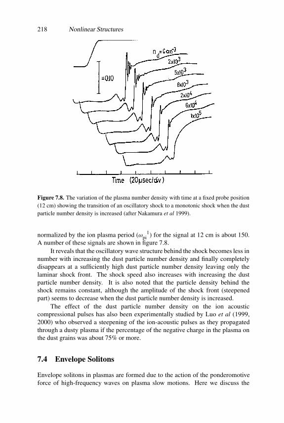
218 Nonlinear Structures
Figure 7.8. The variation of the plasma number density with time at a fixed probe position(12 cm) showing the transition of an oscillatory shock to a monotonic shock when the dustparticle number density is increased (after Nakamura et al 1999).
normalized by the ion plasma period (ω−1pi ) for the signal at 12 cm is about 150.
A number of these signals are shown in figure 7.8.It reveals that the oscillatory wave structure behind the shock becomes less in
number with increasing the dust particle number density and finally completelydisappears at a sufficiently high dust particle number density leaving only thelaminar shock front. The shock speed also increases with increasing the dustparticle number density. It is also noted that the particle density behind theshock remains constant, although the amplitude of the shock front (steepenedpart) seems to decrease when the dust particle number density is increased.
The effect of the dust particle number density on the ion acousticcompressional pulses has also been experimentally studied by Luo et al (1999,2000) who observed a steepening of the ion-acoustic pulses as they propagatedthrough a dusty plasma if the percentage of the negative charge in the plasma onthe dust grains was about 75% or more.
7.4 Envelope Solitons
Envelope solitons in plasmas are formed due to the action of the ponderomotiveforce of high-frequency waves on plasma slow motions. Here we discuss the

Envelope Solitons 219
formation of a Langmuir wave envelope soliton in an unmagnetized dusty plasmawithout considering the dust charge fluctuation effect.
The nonlinear coupling between a large-amplitude Langmuir pump withnon-resonant DA perturbations gives rise to an envelope of Langmuir waveswhich is governed by
∂nel
∂ t+ ∇ · [(ne0 + nes)vl] = 0 (7.4.1)
∂vl
∂ t= − e
meEl − 3V 2
Te
ne0∇nel (7.4.2)
and∇ · El = −4πenel (7.4.3)
where nel and nes are small electron number density perturbations associated withLangmuir and DA waves, respectively and El is the Langmuir wave electric field.Combining equations (7.4.1)–(7.4.3) we obtain the Langmuir wave equation inthe presence of the DA perturbations
∂2 El
∂ t2− 3V 2
Te∇2 El + ω2pe
(1+ nes
ne0
)El = 0. (7.4.4)
We assume that the Langmuir wave electric field varies on the spatio-temporalscales of the DA perturbations. Thus, letting El = E(r, τ ) exp(−iω0t + ik0 · r),where ω0 = (ω2
pe+ 3k20V 2
Te)1/2 ∼ ωpe, in equation (7.4.4) we obtain the envelope
equation
2iω0
(∂
∂τ+ vg0 · ∇
)E + 3V 2
Te∇2 E − ω2pe
nes
ne0E = 0 (7.4.5)
where in the spirit of the slowly varying envelope approximation we have∂E/∂τ � ω0. The Langmuir wave group velocity is denoted by vg0 =3V 2
Tek0/ωpe.The electron number density perturbation nes associated with the DA
perturbations is obtained by averaging the inertialess electron momentumequation over the Langmuir wave period (= 2π/ω0). The result is
me
4∇|vl|2 ∼= e2
4meω2pe∇|E|2 = e∇φs − kBTe
ne0∇nes (7.4.6)
where the left-hand side represents the Langmuir wave ponderomotive force. Thelatter is transmitted to the ions and dust grains through the DA wave potential φs .The ion and dust number density perturbations are determined from
0 = −e∇φs − kBTi
ni0∇nis (7.4.7)
220 Nonlinear Structures
and∂2nds
∂τ 2− qd0nd0
md∇2φs = 0. (7.4.8)
For long-wavelength (in comparison with λD) DA perturbations, we can use thequasi-neutrality condition (enis = enes−qd0nds) and equations (7.4.7) and (7.4.8)to obtain
∂2nes
∂τ 2+ ni0e
kBTi
(∂2
∂τ 2− C2
Di∇2
)φs = 0. (7.4.9)
Substituting for φs from equation (7.4.6) into equation (7.4.9) we have the drivenDA wave equation(
∂2
∂τ 2− C2
DA∇2
)nes
ne0= − 1
1+ δn
(∂2
∂τ 2− C2
Di∇2
)|E|2
16πne0kBTe(7.4.10)
where C2DA = C2
Di/(1 + δn) and δn = ne0Ti/ni0Te. For δn � 1 equation (7.4.10)gives
nes
ne0= − |E|2
16πne0kBTe(7.4.11)
which shows the formation of an electron density cavity by the ponderomotiveforce of the Langmuir waves in a collisionless dusty plasma. Insertingequation (7.4.11) into equation (7.4.5) we obtain the cubic nonlinear Schrodingerequation
2iω0
(∂
∂τ+ vg0 · ∇
)E + 3V 2
Te∇2 E + ω2pe|E|2 E = 0 (7.4.12)
where the Langmuir wave electric field is normalized by (16πne0kBTe)1/2.
Equation (7.4.12) exhibits collapse of Langmuir waves in a sphericalsymmetric situation (Zakharov 1972). However, in one-space dimension, thestationary solution of equation (7.4.12) can be obtained by introducing E =zE(z) exp[iϑ1(τ )+ iϑ2(z)], where ϑ1(τ ) and ϑ2(z) are some constants. Hence, inthe steady-state, equation (7.4.12) can be written as
3λ2De∂2E
∂z2 − λlE + |E|2E = 0 (7.4.13)
where λl = (2/ωpe)(∂ϑ1/∂τ) + 24k20zλ
2De is a nonlinear frequency shift and
ϑ2(z) = 2k0zz. A possible localized solution of equation (7.4.13) is
E = Em sech( z
L
)(7.4.14)
where Em is the maximum normalized amplitude of the envelope soliton andλl = E2
m. The width of the envelope soliton is
L = λDe
(6
Em
)1/2
. (7.4.15)
Vortices 221
The corresponding electron density depletion is
nes
ne0= −|Em|2 sech2
( z
L
). (7.4.16)
Thus, a Langmuir envelope soliton consists of a bell shaped electric field envelopethat is trapped in a self-created density cavity in a dusty plasma.
7.5 Vortices
Coherent vortices appear in two-dimensional fluids and magnetized plasmas. Ina simplest possible scenario, the vortex dynamics is governed by the NS equationwhich admits a monopolar vortex (Hasegawa 1985). However, in a magnetizeddusty plasma we have the possibility of vortices comprising a dipolar (Bharuthramand Shukla 1992b), a tripolar, and a chain (Vranjes et al 2001). Here thevortices are associated with nonlinear dispersive waves that possess, at least, atwo-dimensional character. When the velocity of the fluid (or plasma particles)motion associated with the dispersive waves become locally larger than the wavephase velocity because of the nonlinear effects, one encounters a curving of thewave front which lead to the formation of a two-dimensional travelling vortexstructure. In this section, we discuss the properties of vortices in a non-uniformdusty magnetoplasma.
7.5.1 Electrostatic vortices
We have shown in chapter 4 the existence of a low-frequency (in comparisonwith the ion gyrofrequency) Shukla–Varma (SV) mode (Shukla and Varma 1993)that involves two-dimensional electron and ion motions in a non-uniform dustymagnetoplasma containing stationary dust grains. We now discuss possiblevortex solutions involving nonlinear SV modes. In the presence of low-frequency(namely ωcd , ωpd � |d/dt| � ωci) electrostatic waves, the electron and ionvelocities in our collisionless cold dusty plasma are, respectively
ve ≈ c
B0z × ∇φ (7.5.1)
and
vi ≈ c
B0z × ∇φ − c
B0ωci
(∂
∂ t+ c
B0z × ∇φ · ∇
)∇⊥φ (7.5.2)
where the dynamics of the electrons and ions parallel to zB0 has been neglected.The last term in the right-hand side of equation (7.5.2) represents the nonlinearion polarization drift (Hasegawa and Mima 1978). It comes from the advectionterm (vi · ∇vi) in the ion momentum equation. Substituting equations (7.5.1) and(7.5.2) into the electron and ion continuity equations, letting n j = n j0 + n j1,

222 Nonlinear Structures
where n j1 � n j0, and subtracting the ion continuity equation from that of theelectrons, we obtain after using ne1 = ni1(
∂
∂ t+ c
B0z ×∇φ · ∇
)∇2⊥φ + usv
∂φ
∂y= 0 (7.5.3)
which governs the nonlinear dynamics of the SV modes. Here we have denotedusv = ωci Kqn . In a uniform magnetoplasma, equation (7.5.3) takes the form(
∂
∂ t+ c
B0z × ∇φ · ∇
)∇2⊥φ = 0 (7.5.4)
which is the NS equation governing the dynamics of two-dimensional convectivecells in a collisionless plasma. Equation (7.5.4) admits dual cascading and amonopolar vortex (Hasegawa 1985). The presence of the inhomogeneous term(the third term) in the left-hand side of equation (7.5.3) provides the possibility ofa stationary dipolar vortex structure, as discussed below.
We seek a solution of the generalized NS equation (7.5.3) in the stationaryframe ξ = y − ut , where u is the translational speed of the vortex. Thus,equation (7.5.3) takes the form
u∂
∂ξ∇2⊥φ − usv
∂φ
∂ξ− c
B0J (φ,∇2⊥φ) = 0 (7.5.5)
where the Jacobian is denoted by
J (φ,∇2⊥φ) =(∂φ
∂x
∂
∂ξ− ∂φ
∂ξ
∂
∂x
)∇2⊥φ (7.5.6)
with ∇2⊥φ = (∂2φ/∂x2)+ (∂2φ/∂ξ2). Equation (7.5.5) is satisfied by the Ansatz
∇2⊥φ = C1φ + C2x (7.5.7)
provided that the constants C1 and C2 are related by uC1 − usv − (c/B0)C2 = 0.The double vortex solution of equation (7.5.7) can be constructed followingstandard methods (Larichev and Reznik 1976). Accordingly, we divide the (r, θ)plane into outer (r > Rv) and inner (r < Rv) regions, where r = (x2 + ξ2)1/2
and θ = arctan(ξ/x) are the polar coordinates and Rv corresponds to the vortexradius. For localized solutions we must have C2 = 0 in the outer region so thatCo
1 = usv/u ≡ k20. The outer region solution is
φo(r, θ) = φ0 K1(k0r) cos θ (7.5.8)
where φ0 is a constant and K1 is the modified Bessel function of the first kind.Thus a well-behaved outer solution is possible for k2
0 > 0, which is satisfied forusv > 0. The inner region solution is
φi =[φi J1(kir)+ Cv
k2i
r
]cos θ (7.5.9)
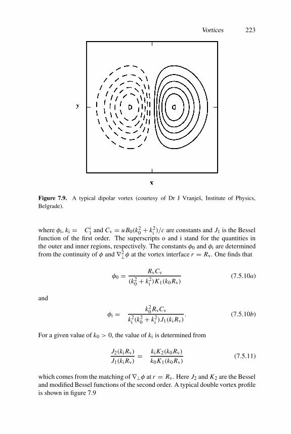
Vortices 223
Figure 7.9. A typical dipolar vortex (courtesy of Dr J Vranjes, Institute of Physics,Belgrade).
where φi, ki = −C i1 and Cv = u B0(k2
0 + k2i )/c are constants and J1 is the Bessel
function of the first order. The superscripts o and i stand for the quantities inthe outer and inner regions, respectively. The constants φ0 and φi are determinedfrom the continuity of φ and ∇2⊥φ at the vortex interface r = Rv. One finds that
φ0 = RvCv
(k20 + k2
i )K1(k0 Rv)(7.5.10a)
and
φi = − k20 RvCv
k2i (k
20 + k2
i )J1(ki Rv). (7.5.10b)
For a given value of k0 > 0, the value of ki is determined from
J2(ki Rv)
J1(ki Rv)= − kiK2(k0 Rv)
k0K1(k0 Rv)(7.5.11)
which comes from the matching of∇⊥φ at r = Rv. Here J2 and K2 are the Besseland modified Bessel functions of the second order. A typical double vortex profileis shown in figure 7.9
224 Nonlinear Structures
7.5.2 Electromagnetic vortices
We now discuss electromagnetic vortices (Pokhotelov et al 1999) that involvenonlinear low-frequency (in comparison with the ion gyrofrequency), long-wavelength (in comparison with the ion gyroradius) electromagnetic waves in anon-uniform dusty magnetoplasma containing a density inhomogeneity along thex-axis. The dust component is considered to be immobile. In the electromagneticfields, the electron and ion fluid velocities in a warm dusty plasma are
ve ≈ c
B0z ×∇φ − ckBTe
eB0nez ×∇ne + vez
(z + ∇Az × z
B0
)(7.5.12)
and
vi ≈ c
B0z ×∇φ + ckBTi
eB0niz ×∇ni − c
B0ωci
(∂
∂ t+ vi ·∇
)∇⊥φ (7.5.13)
where the parallel component of the electron fluid velocity is given by (cfequation (4.7.18))
vez ≈ c
4πnee∇2⊥Az (7.5.14)
where we have ignored the ion motion parallel to z as well as neglected thecompressional magnetic field perturbation. Thus, the DIA and magnetosonicwaves are decoupled in our low-β (β � 1) dusty plasma system.
Substituting equation (7.5.12) into the electron continuity equation, lettingn j = n j0(x)+ n j1, where n j1 � n j0 and using equation (7.5.14) we obtain
dne1
dt− c
B0
∂ne0
∂x
∂φ
∂y+ c
4πe
d∇2⊥Az
dz= 0, (7.5.15)
where d/dt = (∂/∂ t)+(c/B0) z×∇φ·∇ and d/dz = (∂/∂z)+B−10 ∇Az× z·∇. We
have assumed vE B · ∇ � vez∂/∂z, which implies that (ω2pe/ωce)| z ×∇φ ·∇| �
c∂z∇2⊥Az . On the other hand, substitution of the ion fluid velocity, given byequation (7.5.13) into the ion continuity equation yields
dni1
dt− c
B0
∂ni0
∂x
∂φ
∂y− cni0
B0ωci
(d
dt+ ui∗
∂
∂y
)∇2⊥φ
− c2kBTi
eB20ωci
∇⊥ · [( z ×∇ni1) ·∇∇⊥φ] = 0 (7.5.16)
where ui∗ = (ckBTi/eB0ni0)∂ni0/∂x is the unperturbed ion diamagnetic driftspeed. Subtracting equation (7.5.16) from equation (7.5.15) and assuming ni1 =ne1, we obtain the modified ion vorticity equation(
d
dt+ ui∗∂y
)∇2⊥φ +
V 2A
c
d∇2⊥ Az
dz+ usv
∂φ
∂y
+ ckBTi
eB0ni0∇⊥ · [( z ×∇ne1) ·∇∇⊥φ] = 0. (7.5.17)

Vortices 225
By using equations (7.5.12) and (7.5.14), the parallel component of the electronmomentum equation can be written as
(∂
∂ t+ ue∗
∂
∂y
)Az − λ2
ed∇2⊥Az
dt+ c
dφ
dz− ckBTe
ene0
dne1
dz= 0 (7.5.18)
where ue∗ = −(ckBTe/eB0ne0)∂ne0/∂x is the unperturbed electron diamagneticdrift speed.
Let us now seek stationary solutions (Pokhotelov et al 1999) of the nonlinearequations (7.5.15), (7.5.17) and (7.5.18) by assuming that all the field variablesdepend on x and η = y + αz − ut , where α represents the angle between thewavefront normal and the (x, y) plane. Two cases are considered.
7.5.2.1 Warm plasma
In the stationary η-frame, equation (7.5.18) for λ2e |∇2⊥| � 1 can be written as
DA
(φ − kBTe
ene0ne1 − u − ue∗
αcAz
)= 0 (7.5.19)
where DA = (∂/∂η)+(1/αB0)[(∂Az/∂η)(∂/∂x)−(∂Az/∂x)(∂/∂η)]. A solutionof equation (7.5.19) is (Liu and Horton 1986)
ne1 = ne0e
kBTeφ − (u − ue∗)ne0e
αckBTeAz . (7.5.20)
Writing equation (7.5.15) in the stationary frame and making use ofequation (7.5.20) it can be put in the form
DA
[λ2
De∇2⊥Az + u(u − ue∗)α2c2 Az − u − ue∗
αcφ
]= 0. (7.5.21)
A solution of equation (7.5.21) is
λ2De∇2⊥Az + u(u − ue∗)
α2c2Az − u − ue∗
αcφ = 0. (7.5.22)
The modified ion vorticity equation (7.5.17) for cold ions can be expressed as
Dφ(∇2⊥φ − k20φ)−
V 2Aα
cuDA∇2⊥Az = 0 (7.5.23)
where Dφ = (∂/∂η)− (c/u B0)[(∂φ/∂x)(∂/∂η)− (∂φ/∂η)(∂/∂x)]. Combiningequations (7.5.22) and (7.5.23) we obtain
Dφ
(∇2⊥φ +
p
ρ2sφ + u − ue∗
αcρ2s
Az
)= 0 (7.5.24)

226 Nonlinear Structures
where p = (CS/u)[Kdρs+(ue∗−u)/CS]. A typical solution of equation (7.5.24)is
∇2⊥φ +p
ρ2sφ + u − ue∗
αcρ2s
Az = C3
(φ − u B0
cx
)(7.5.25)
where C3 is an integration constant. Eliminating Az from equations (7.5.22)and (7.5.25), we obtain a fourth-order inhomogeneous differential equation(Pokhotelov et al 1999)
∇4φ + F1∇2⊥φ + F2φ + C3u2(u − ue∗)B0
α2c3λ2De
x = 0 (7.5.26)
where F1 = (p/ρ2s ) − C3 + u(u − ue∗)/α2c2λ2
De and F2 = [(u −ue∗)2/α2c2λ2
Deρ2s ] + (p − C3ρ
2s )u(u − ue∗)/α2c2λ2
Deρ2s . We note that in the
absence of charged dust we have usv = 0 and F2 = 0 in the outer region whenC3 = 0. In such a situation, the outer region solution of equation (7.5.26) wouldhave a a long tail (decaying as 1/r ) for (u − ue∗)(α2V 2
A − u2) > 0 (Liu andHorton 1986). On the other hand, inclusion of a small fraction of dust grainswould make F2 finite in the outer region. Here we have the possibility of well-behaved solutions. In fact, equation (7.5.26) admits spatially bounded dipolarvortex solutions. In the outer region (r > Rv), we set C3 = 0 and obtain thesolution of equation (7.5.26) as (Liu and Horton 1986)
φo = [Q1 K1(s1r)+ Q2 K1(s2r)] cos θ (7.5.27)
where Q1 and Q2 are constants and s21,2 = −[−α1 ± (α2
1 − 4α2)1/2/2] for
α1 < 0 and α21 > 4α2 > 0. Here, α1 = (p/ρ2
s ) + u(u − ue∗)/α2c2λ2De and
α2 = [(u − ue∗)2 + u(u − ue∗)p]/α2c2λ2Deρ
2s . In the inner region (r < Rv), the
solution reads
φi =[
Q3 J1(s3r)+ Q4 I1(s4r)− C i3
λ2De
u2(u − ue∗)B0
α2c3 F i2
r
]cos θ (7.5.28)
where Q3, Q4, C i3 and F i
2 are constants. We have defined s3,4 = [(Fi21 −4F i
2)1/2±
F i1]/2 for F i
2 < 0. Thus, the presence of charged dust grains is responsible for thecomplete localization of the vortex solutions in the outer as well as in the innerregions of the vortex core.
7.5.2.2 Cold plasma
We now present the double vortex solution of equations (7.5.17) and (7.5.18) inthe cold plasma approximation. Hence we set Tj = 0 and write equations (7.5.17)in the form of equation (7.5.23), while equation (7.5.18) in the stationary framecan be expressed as
Dφ
[(1− λ2
e∇2⊥)Az − αc
uφ]= 0. (7.5.29)

Vortices 227
It is easy to verify that equation (7.5.29) is satisfied by
(1− λ2e∇2⊥)Az − αc
uφ = 0. (7.5.30)
By using equation (7.5.30) one can eliminate ∇2⊥Az from equation (7.5.23),obtaining
Dφ
[∇2⊥φ − k2
0φ +α2V 2
A
c2λ2eφ − αV 2
A
ucλ2e
Az
]= 0. (7.5.31)
A typical solution of equation (7.5.31) is
∇2⊥φ + β1φ − β2 Az = C4
(φ − u B0
cx
)(7.5.32)
where β1 = (α2V 2A/u2λ2
e) − k20, β2 = αV 2
A/ucλ2e and C4 is an integration
constant. Eliminating Az from equations (7.5.30) and (7.5.32) we obtain
∇4⊥φ + G1∇2⊥φ + G2φ − C4u B0
λ2ec
x = 0 (7.5.33)
where G1 = λ−2e [(α2V 2
A/c2) − 1] − k20 − C4 and G2 = (C4 − k2
0)/λ2e .
Equation (7.5.33) is similar to equation (7.5.26) and its bounded solutions (similarto equations (7.5.27) and (7.5.28)) exist provided that u2(1+ k2
0λ2e) > α2V 2
A andusv > 0. In the absence of dust, we have G2 = 0 in the outer region (C4 = 0),and the outer region solution of equation (7.5.33) for the dust-free case also hasa long tail. The various constants appearing in the section 7.5.2 are contained inLiu and Horton (1986).

Chapter 8
Dust Crystals
8.1 Preamble
In his classic paper Wigner (1938) showed that upon cooling an electron gascan condense and form an ordered crystalline structure, the so-called ‘Wignercrystal’. The formation of a Wigner crystal (as well as crystallization of a quantumelectron fluid) has been investigated experimentally. The crystal structureswere also observed in electrostatic vacuum traps or charged macroparticlesand in Paul and Penning traps with Mg and Be ions that are cooled to verylow temperatures (∼10−3 K). A Coulomb crystal is also realized in colloidalsuspensions. The colloidal crystals consist of almost mono-dispersive micron-sized particles suspended in an electrolyte where they become charged negatively,having electron charges as high as 103–104. The particles are screened by ionsof both signs in the electrolyte. The Coulomb interaction between the particlesrenders the formation of a crystal structure energetically more favourable. Astrong coupling between the particles takes place at distances less than thescreening radius, which in colloidal suspensions is very small. This leads to theresult that for crystallization rather high particle number density (Np ∼ 1012)is necessary. Consequently, colloidal crystals are usually opaque, hindering anexperimental study of their bulk properties. The drawback of the colloidal crystalsis that they have a long equilibrium relaxation time, amounting to several weeks.
Condensation or self-organization in a many-particle system occurs providedthat the potential due to nearest neighbouring forces is (substantially) largerthan the thermal energy of the particles. Assuming that Coulomb collisions aredominant in our plasma, we can express the coupling parameter as
� j �q2
j n1/3j
kBTj≥ 1. (8.1.1)
When we consider an electron–ion plasma with multiply charged ions, we have
228

Preamble 229
(Morfill et al 1999a)
�e � e2n1/3e
kBTe(8.1.2)
and
�i � Z2i e2n1/3
i
kBTi. (8.1.3)
Now invoking the quasi-neutrality condition (Z ini = ne) and putting Te = Ti, weobtain
�i � Z5/3i �e (8.1.4)
which indicates that the Coulomb coupling increases with the charge state ofthe ions. The electrons rearrange themselves around the ions to effectivelyshield the excess charge over the electron Debye radius λDe. Subsequently, theCoulomb interaction potential in equation (8.1.1) has to be modified to includethis shielding. We then obtain, instead of equation (8.1.3)
�i � Z2i e2n1/3
i
kBTiexp(−κi) (8.1.5)
where κi is the ratio of the inter-ion distance (�n−1/3i ) to the electron Debye
radius, i.e.
κi = 1
n1/3i λDe
. (8.1.6)
The quasi-neutrality condition along with κi � 1 leads to a strong couplingcondition (Morfill et al 1999a)
Z i > 4πTi
Te�i. (8.1.7)
This means that to have a strongly coupled plasma (�i ≤ 1 and Ti � Te), theions have to be at least fourfold ionized. Furthermore, for plasma condensation(�i > 172 and Ti � Te), we should have Z i > 50. This is impossible for an idealelectron–ion plasma. The fluctuation in Z i introduces a corresponding fluctuationin the Coulomb potential between neighbouring ions, which is proportional toZ i1 Z i2. This will increase the effective thermal energy of the ions and lower �i.Hence, if the distribution of the charge state is too wide, plasma condensationwill be prevented. However, the strong coupling condition is easier to satisfyif the plasma ions (or at least one of the plasma particle constituents, e.g. dust)are multiply charged. Thus, as we defined in equation (1.2.17), the shieldingof a dust particle by the other plasma particles (electrons and ions) introducesanother important parameter (the ratio between the inter-particle separation a �n−1/3
d and the Debye radius λD) κd � 1/n1/3d λD. Ikezi (1986) considered this
screening effect and theoretically predicted the possibility of crystallization of a

230 Dust Crystals
Figure 8.1. Parameter ranges for different kinds of plasmas in the universe. The solid lineshows the � = 1 line, which marks the transition from strongly to weakly coupled plasmas(after Morfill et al 1999a).
dust subsystem in a non-equilibrium gas discharge plasma when the Coulombcoupling parameter
�d = Z2de2n1/3
d
kBTdexp(−κd) (8.1.8)
is larger than 172. It turns out that because of the large amount of dust graincharges (higher values of Zd) and lower dust temperature, it is more likely tohave a significantly large �d value in a dusty plasma in comparison with the �ivalue in an electron–ion plasma. Figure 8.1 depicts the parameter regimes thatare applicable to different kinds of weakly and strongly coupled plasmas in spaceand laboratories (Morfill et al 1999a).
About eight years after the publication of Ikezi’s paper, the formation of dustcrystals were finally observed experimentally in a high-frequency discharge nearthe lower electrode in the boundary of the near-cathode region (Chu and I 1994,

Properties of Plasma Crystals 231
Thomas et al 1994, Hayashi and Tachibana 1994, Melzer et al 1994). The dustcrystals were also observed in the strata of a stationary glow discharge (Fortov etal 1997).
The Coulomb dust crystals consist of ordered arrangements of micron-sizeddust grains (or rods) in low-temperature partially ionized plasmas. A dustyplasma crystal can have a varied crystal structure, with a lattice constant of theorder of a fraction of a millimetre, which makes it possible to observe it underlight illumination with the naked eye. The dusty plasma crystals possess manyvirtues, making them an indispensable diagnostic tool not only for the study ofhighly non-ideal plasmas, but also for the study of the fundamental properties ofcrystals. These include simplicity of dust crystal fabrication, observation andeasy parameter control, their rapid equilibrium relaxation times and responsetimes to external perturbations, etc. The dusty plasma crystals represent abridge between atomic or molecular clusters and bulk materials and thus havethe potential of elucidating fundamental aspects of micro- and macro-physicalmaterial properties. They open new perspectives for creating new materials whichcan be utilized for advanced schemes of radiation sources. The dusty plasmacrystals can be used as macroscopic model systems for studying dislocations,phase transitions, annealing, wave propagation, etc. They also appear to beparticularly suited as model systems for ‘nanocrystals’ with only a few latticeplanes. The formation of dusty plasma crystals and their stability, growth,melting, etc may be of importance in plasma processing devices used in micro-electronics fabrications and integrated circuits where ‘dust contaminants’ insidethe reactors play a crucial role in causing defects. The presence of smallerparticulates in plasma technology can cause wafer contamination and break-down. Therefore, control of this contamination is of major importance forindustry as well.
In this chapter, we discuss the formation of ordered structures of chargedmacroparticles of various sizes in rf and glow discharges. We study the influenceof the discharge parameters on the possibility of the existence of quasi-crystallinestructures of dust particles along with the conditions for their formation anddestruction. We also consider some important questions related to different formsof potentials associated with the interactions between macroparticles, as well asto the generation of Mach cones in dusty plasmas.
8.2 Properties of Plasma Crystals
The properties of dusty plasma crystals have to be evaluated in relation toother crystal systems. In their review papers, Morfill et al (1997, 1999a) havehighlighted common properties as well as differences, which are summarizedbelow.
• Contrary to ion crystals, which are produced in traps or storage rings, dustyplasma crystals are easily produced in rf and dc plasma discharges as table-
232 Dust Crystals
top experiments even at room temperature.• Characteristic timescales for plasma crystal formation are of the order of
one second. This very fast response (about a million times faster than that ofcolloidal suspensions) allows investigations of dynamical properties whichwere not accessible before.
• Plasma crystals consist of negatively charged microspheres, ions, andelectrons. A Coulomb crystal in a plasma is usually formed around theplasma sheath boundary owing to the transport of particles to a balancedposition by the resultant of the electrostatic force, ion drag force and gravity.In space-under microgravity conditions, larger three-dimensional systemscan be formed and investigated in much weaker electric fields than thosenecessary for dust levitation on the ground. This unique situation allowsthe study of weak processes, namely surface tension, dipolar binding forces,shear effects etc, and controlled conditions for the investigation of criticalphenomena. Gravity does not play a role for ion crystals, whereas forcolloidal or surface crystals (e.g. Langmuir–Blodgett films) it is compensatedby a suitable suspension medium, which may then lead to a heavy dampingand a very long equilibration time.
• Plasma crystals are easy to control in laboratories. One can fabricate singlehexagonal cells, linear chains, monolayer as well as flat multi-layer dustcrystals with several thousand cells. Large fine particle crystals are alsoformed during the chemical reactions between silane and oxygen gases.
• The vertical positions of dusty plasma crystals in the electrostatic sheathcan also be controlled, e.g. by using ultraviolet radiation. This may bequite important for testing the plasma crystal properties under conditions ofvariable ion flow. In rf discharges, the ions are accelerated towards the lowerelectrode in the sheath. At the edge of the main plasma this flow velocity isnearly thermal, but closer to the electrode it becomes highly super-thermal.
• Dusty plasma crystals are easily visualized using laser illumination and aCCD camera. In this way, a full three-dimensional monitoring is possible.The easy visualization, including direct storage and computer analysis,significantly enhances our diagnostic capacity with respect to the othercrystal systems and makes a number of scientific investigations possible.
• Plasma crystals are easily manipulated by external electromagnetic forces.This opens up the possibility to perform active experiments serving carefullydesigned purposes.
• The variety of plasma crystals that can be produced is large. The plasmaparameters (mass, density, temperature, gas pressure) play a role, asdo the rf power input, microsphere size, shape, density and electricalproperties.
• The propagation and damping of dust lattice waves (with the frequency ofseveral Hz) is also possible in a plasma crystal, similar to the solid stateionic crystals.
• Compared with liquid colloid systems, strongly coupled dusty systems

Potential of a Test Charge 233
have considerably less damping (about a factor of a million—depending onthe neutral gas pressure). This allows the investigations of processes ontimescales not previously accessible for experimental studies, in particularthe investigation of critical phenomena, such as phase transitions.
• A Coulomb crystal in a particle plasma is, however, superior to others in amodel of an atomic crystal because of the large lattice constant and stronginteractions. The latter include new types of attractive forces (namely asso-ciated with wake fields) between like particles.
8.3 Potential of a Test Charge
A dust particle in a plasma usually acquires huge electric charges and interactswith other dust particles. The interaction potential between macroscopic dustparticles depends on their own physical parameters and those of the ambientplasma. The question of the correct potential between dust particles is not purelyfundamental and still remains open (Konopka et al 2000). The plasma flowanisotropies, dipole effects (Lapenta 1999) for larger dust particles and long-range attractive interactions due to wakefield (Nambu et al 1995, Shukla and Rao1996) and shadowing effects (Tsytovich et al 1996, Lampe et al 2000) may playsignificant roles. To understand the behaviour of dusty plasmas in complicatedsituations, however, the results for simple and basic cases are indispensable. Wenow discuss various forms of the test charge potential in a dusty plasma.
Nearly four decades ago, Neufeld and Ritchie (1955) wrote an elegant paperdealing with the passage of charged particles through a plasma. They calculatedthe potential distributions of a test particle in an electron plasma with fixed ionbackground and pointed out their importance to the energy loss. Montgomery etal (1968) demonstrated that the far-field potential of a moving test charge in auniform electron–ion plasma decreases as the inverse cube of the distance r fromthe test charge. On the other hand, the far-field potential in a collisional electron–ion plasma (Stenflo et al 1973) may decay as r−2. The test charge potentialcalculation has been further extended by Chen et al (1973) by incorporating theion dynamics. The latter allows the possibility of far-wake structures in rarefiedplasma flows past charged bodies. The wakefield in an electron–ion plasma hasalso been found by Nambu and Akama (1985).
We consider the potential of a test particle in a homogeneous, isotropic dustyplasma. The electric potential of a test particle (with charge qt) moving with aconstant velocity v0 is (Krall and Trivelpiece 1973)
φ(R, t) = qt
2π2limε→0
∫dk
exp(ik · r − εk)
k2 D(k,−k · v0)(8.3.1)
where r = R − v0t and D(k,−k · v0) is the dielectric function of the dustyplasma. Following Montgomery et al (1968), the term limε→0 exp(−εk) has beenincluded to ensure proper convergence of the integrals.

234 Dust Crystals
The calculation of the dielectric function for longitudinal disturbances in adusty plasma has been carried out in chapter 4. The dielectric function is of theform
D(k,−k · v0) = 1+ χe + χi + χd + χq. (8.3.2)
We consider the parameter regimes kVTd � |k · v0| � νen,in � kVTe,Ti, andobtain the dielectric susceptibilities as
χe ≈ k2De
k2
[1− i
√π
2
k · v0
kVTe
(1+ νen
kVTe
)](8.3.3)
χi ≈ k2Di
k2
[1− i
√π
2
k · v0
kVTi
(1+ νin
kVTi
)](8.3.4)
χd = −ω2
pd
(−k · v0 + iνdn)2(8.3.5)
and
χq =k2
q
k2
ν1
(ν1 − ik · v0). (8.3.6)
Let us consider the case with ωpd � |k · v0| � ν1, so that the dielectric function(8.3.2) takes the form
D(k,−k ·v0) ≈ 1+ k20
k2− i
√π
2
∑j=e,i
k · v0k2D j
k3VT j
(1+ ν jn
kVT j
)− i
k2q
k2
k · v0
ν1(8.3.7)
where k20 = k2
D + k2q ≡ 1/λ2
0. Since our test charge is supposed to move veryslowly, namely |v0| � VTe,Ti, we have from equation (8.3.7)
1
D(k,−k · v0)≈ k2λ2
0
1+ k2λ20
+ ik4λ4
0
(1+ k2λ20)
2
×[√
π
2
∑j=e,i
k · v0k2D j
k3VT j
(1+ ν jn
kVT j
)+ k2
q
k2
k · v0
ν1
]. (8.3.8)
Substituting equation (8.3.8) into equation (8.3.1) and carrying out the integrationin a straightforward manner, we readily obtain (Shukla and Stenflo 2001b)
φ ≈ qt
rexp
(− r
λ0
)+ qtv0
(α2
r2 +α3
r3 +α4
r4
)cos γ (8.3.9)
where α2 ≈ ∑ν jnk2
D jλ40/V 2
T j , α3 ≈ ∑k2
D jλ40/VT j , α4 ≈ k2
qλ40/ν1, γ is the
angle between r and v0 and r = |R − v0t| is the distance between the testcharge and the observer. The first term in the right-hand side of equation (8.3.9)is the usual Debye shielding term in which the dusty plasma Debye radius is

Attractive Forces 235
reduced by a factor 1/(1 + k2qλ
2D)
1/2 due to the consideration of the dust chargefluctuations. The third term in the right–hand side of equation (8.3.9) is thefar-field potential of a moving test charge caused by Landau damping, whilethe second and fourth terms represent the far-field potentials associated withcollisions (between neutrals and electrons/ions) and the dust charge perturbations,respectively. For large r (� λ0), exp(−r/λ0) can be so small that the first term issmaller than the last three terms in equation (8.3.9).
8.4 Attractive Forces
It is well known that two charged dust particles of similar sign repel each otherbecause of their shielded Coulomb interaction at distances shorter than the dustyplasma Debye radius. This assertion holds as long as the dust grains move fasterthan the electron thermal speed in which case only the interaction between thegrains should be taken into account. This leads to the Debye–Huckel potentialenergy
Ugg = qd1qd2
rexp
(− r
λD
)(8.4.1)
where qd1 and qd2 are the charges of two interacting grains. However, in practicalexperimental conditions, the grains in the plasma are moving so slowly thatthey always carry their Debye sphere due to the adiabatic condition. Such dustgrains are referred to as dressed grains. The interaction potential between twodressed grains contains an attractive part at large distances. Further attractionmechanisms involve the wakefield arising from the coupling between the dustgrains and acoustic modes, the asymmetric bombardment of a dust particle byplasma particles which produce shadowing of this dust particle by neighbouringones, Coulomb scattering of charged plasma particles by charged dust particles,induced dipole moment created around an isolated dust grain, etc. Let us nowdescribe some of these attractive forces.
8.4.1 Electrostatic energy between dressed grains
The electrostatic energy between two dressed grains should include four termscorresponding to that between two grains, two Debye spheres and a grain-Debyesphere (two cross terms). The relevant electrostatic energies are then the sum ofUgg, Udd and Ugd. The sum of the electrostatic energies associated with the twoDebye and grain-Debye spheres (namely Udd +Ugd ≡ Usd) can be deduced fromthe expression (Wang 1999)
Usd = −∫ −∞
0
∫ 2π
0
∫ π
0ρ2 dρ sin θ dθ dϕ
q1d exp(−ρ/r)
4πρλ2D
q2d exp(−ρ′/λD)
ρ′(8.4.2)
236 Dust Crystals
where ρ′ = √r2 + ρ2 − 2rρ cos θ . Carrying out the integration in
equation (8.4.2) we readily obtain
Usd = −q1dq2d
2λDexp
(− r
λD
). (8.4.3)
By adding equations (8.4.1) and (8.4.3) we obtain the total electrostatic energy(Resendes et al 1998, Wang 1999)
UT = q1dq2d
rexp
(− r
λD
)(1− r
2λD
). (8.4.4)
The potential UT is much sharper than the Debye potential near the origin. It hasa zero point at r/λD = 2 and attains a minimum value (−0.0087q1dq2d/λD) atr/λD ≈ 2.732. Two dressed grains may attract each other when the intergraindistance is greater than 2.732λD.
8.4.2 Wake potentials
It has been shown theoretically by Nambu et al (1995) that collective interactionsinvolving very low-frequency electrostatic waves in dusty plasmas can give riseto an oscillatory wake potential (Shukla and Rao 1996), which may cause grainattraction. The phonons in a dusty plasma are replaced by the DA and DIAoscillations. The resonance interaction between a test particle and these dustyplasma modes gives rise to an oscillatory wakefield. In the negative potentialregion of the wakefield, the ions are focused and they provide a possibilityfor attracting negatively charged dust grains in a linear chain. This proposedmechanism of the charged dust grain attraction is analogous to the Cooperpairing (de Gennes 1966) of electrons which are glued by phononic motions insuperconductors.
To calculate the potential of a test charge including the wakefield effects,one should start from equation (8.3.1) by employing a general form of the plasmasusceptibility χ j , as given by equation (5.5.2). However, in order to illustrate thephysics of the wakefield, we consider a collisionless dusty plasma.
8.4.2.1 Unmagnetized dusty plasmas
We consider two types of electrostatic responses in a collisionless dusty plasma byignoring Landau damping. First, we assume the presence of ultra low-frequencyDA waves for which the dielectric constant takes the form
D(k, ω) = 1+ 1
k2λ2D
− ω2pd
ω2. (8.4.5)
Second, we consider the DIA waves for which the dielectric constant reads
D(k, ω) = 1+ 1
k2λ2De
− ω2pi
(ω − k · vi0)2. (8.4.6)

Attractive Forces 237
The inverse of the dielectric response function associated with the DA waves,obtained from equation (8.4.5), is
1
D(k, ω)= k2λ2
D
1+ k2λ2D
(1+ ω2
da
ω2 − ω2da
)(8.4.7)
where ωda = kCD/(1 + k2λ2D)
1/2 is the frequency of the DA waves. Similarly,from equation (8.4.6) we readily obtain
1
D(k, ω)= k2λ2
De
1+ k2λ2De
[1+ ω2
di
(ω − k · vi0)2 − ω2di
](8.4.8)
where ωdi = kCS/(1+ k2λ2De)
1/2 is the frequency of the DA waves.If we substitute equations (8.4.7) and (8.4.8) into equation (8.3.1), besides
the well known Debye–Huckel screening potential of the dusty plasma, namely
φd = qt
rexp
(− r
λD
)(8.4.9)
there appears an additional potential involving collective effects caused by the DAand DIA waves, namely
φc =∫
qt
2π2k2Fw(k, ω) exp(ik · r)δ(ω − k · v0) dk dω (8.4.10)
where
Fw(k, ω) = k2λ2Dω
2da
(1+ k2λ2D)(ω
2 − ω2da)
(8.4.11)
for the DA waves and
Fw(k, ω) = k2λ2Deω
2di
(1+ k2λ2De)[(ω − k · vi0)2 − ω2
di](8.4.12)
for the DIA waves. It follows from equations (8.4.11) and (8.4.12) that thepotential changes its sign due to the over screening-depending upon whether ωis larger or smaller than ωda or ωdi. However, if ω is close to one of thesefrequencies, there appears a strong resonant interaction between the waves and thetest particle. When the latter moves with a velocity slightly larger than the phasevelocity of the DA or DIA waves, the potential behind the test particle oscillatesas a wake. Thus, the formation of quasi-lattice structures is, in principle, possiblebecause there are regions of attractive and repulsive forces between the particlesof the same polarity.
The wake potential arises from the residues at the poles at ω = ±ωda,±ωdi.Thus, following the standard procedure (Nambu and Akama 1985), we canintegrate equation (8.4.10) and obtain the non-Coulombian part of the wake

238 Dust Crystals
potential. For long-wavelength (in comparison with the Debye radius) DA waveswith k⊥ρ � 1 and |z−vt| > λD, where z and ρ are the cylindrical coordinates ofthe field point and k⊥ is the wavenumber component perpendicular to the z axis,the wake potential for a near-field approximation is (Nambu et al 1995)
φc(ρ = 0, z, t) ≈ 2qt
|z − vt| cos
( |z − v0t|Lda
)(8.4.13)
where Lda = λD(v20 − C2
D)1/2/CD is the effective length. When we consider the
DIA wave case with no ion streaming, we have to replace λD and CD by λDe andCS respectively. However, in a plasma with streaming ions (namely vi0 = zui0)we have to use equation (8.4.12). For a static test charge we then obtain (Shuklaand Rao 1996, Nambu et al 1997)
φc(x, t) = qt
2π2λ2DeM2
∫dk⊥ dkz
k2
1+ k2
exp(− k·x
λDe
)(k2
z + k2+)(k2z − k2−)
(8.4.14)
where the wavevector is normalized by λ−1De , M = ui0/Cs , k2 = k2
z + k2⊥,and k± = ±(1/2)(1 − M−2 + k2⊥) + [k2⊥M−2 + (1 − M−2 + k2⊥)2/4]1/2.The oscillating contribution to the collective potential in equation (8.4.14) arisesfrom the residues at the poles at kz = ±k−. The integration over angles inequation (8.4.14) can be carried out by using an expansion in spherical harmonics.The main contribution to the stationary wake potential is
φc(ρ = 0, z) = qt
|z|cos(|z|/Ldi)
1− M−2 (8.4.15)
where Ldi = λDe|M2−1|1/2. It emerges from equations (8.4.13) and (8.4.15) thatthe wake potentials are attractive for cos(|z−v0t|/Lda) < 0 and cos(|z|/Ldi) < 0when the test charge is moving and stationary, respectively. For an effectiveattraction of stationary grains, the speed of the streaming ions should exceed CS,which is usually the case in a plasma sheath. The attractive wake potential candominate over the repulsive (the Debye–Huckel screening) potential because ofthe rapid decrease of the latter beyond the shielding cloud.
Physically, the force of attraction between two electrons (or negativelycharged particulates) is attributed to the polarization of the medium caused bya test electron (negatively charged particulate) which attracts positive ions. Theexcess positive ions, in turn, attract a neighbouring electron (negatively chargedparticulate). Thus, the collective interactions involving phonons (DA and DIAwaves) play an essential role in the Cooper pair mechanism in superconductivityas well as in dusty plasmas. Lampe et al (2000) have carried out computersimulations of the wake potential in a collisionless dusty plasma by using thekinetic ion response. A contour plot of the wake potential is shown in figure 8.2.

Attractive Forces 239
Figure 8.2. A contour plot of φ(r, z) for M = 1.5 and Te/Ti = 25. The grain is at thecentre of the left-most node. The solid curves indicate negative potential while the dashedcurves indicate positive potential. The positive node just behind the grain is by far thestronger potential well (after Lampe et al 2000 and courtesy of G Joyce and M Lampe,NRL, Washington).
8.4.2.2 Magnetized dusty plasmas
Laboratory and astrophysical plasmas are usually held in a static magnetic field.Therefore, it is of practical interest to study the wake potential around a testparticle in the presence of electrostatic waves in a dusty magnetoplasma.
Let us consider a dusty plasma embedded in an external magnetic field zB0.The dielectric constant of the dusty plasma in the presence of EIC waves withkVTi, ωpd, ωcd, ωpikz/k � ω ∼ ωci � kz VTe, ωce is
D(k, ω) = 1+ 1
k2λ2De
− ω2pi
�2 − ω2ci
k2⊥k2 (8.4.16)
where � = ω− k ·vi0. It can be readily shown that the reciprocal of the dielectricconstant is of the form
1
D(k, ω)≈ k2λ2
De
1+ k2λ2De
(1+ ω2
ds
�2 − ω2ci − ω2
ds
)(8.4.17)

240 Dust Crystals
where ωds = k⊥CS/(1 + k2λ2De)
1/2. Now, substituting 1/D (obtained fromequation (8.4.17)) into equation (8.3.1), we have φ = φd + φc, where
φd = qt
rexp
(− r
λDe
)(8.4.18)
is the wellknown Debye–Huckel screening potential and the potential involvingthe EIC waves is
φc = qt
2π2
∫λ2
De
(1+ k2λ2De)
ω2ds
(�2 − ω2ic)
δ(ω − k · v0) exp[ik · (r − v0t)] dk dω
(8.4.19)where ω2
ic = ω2ci + ω2
ds . As mentioned earlier, the potential in equation (8.4.19)changes its sign due to the over-screening depending upon whether |ω − k · vi0|is larger or smaller than ωic. However, if ω is close to k · vi0 ± ωic, there appearsa strong resonant interaction between the EIC waves and the test particle. Whenthe velocity of the latter or the ion streaming velocity is slightly larger than thephase velocity of the EIC waves, the potential behind the test particle oscillatesas a wake. We now present the asymptotic behaviour of the wake potential in twolimiting cases.
(i) We assume that the test particle speed is much larger than the ion streamingspeed. Thus, the main contribution to the wakefield arises from the residuesat the poles at ω = ±ωic ≈ ωci+ k2⊥C2
S/2ωci. Accordingly, we can integrateequation (8.4.19) in a straightforward manner. For long-wavelength (incomparison with λDe and ρs ) EIC oscillations with ξ = |z− vz t| � λDe, ρs ,we obtain the wake potential (Shukla and Salimullah 1996)
φc ≈ qt
ξ
λ2De
ρ2s
cos
(ξ
Lb
)(8.4.20)
where Lb = 2vz/3ωci is the effective attraction length and vz is thez component of vi0. The maximum upper limit of the perpendicularwavelength is taken to be of the order of ρs . Equation (8.4.20) reveals thatφc and Lb are a function of B0.
(ii) When the test dust particulate is stationary, we have for the wake potential
φc = qt
π
λ2DeC2
S
v2iz
∫dkz dk⊥
k3⊥ J0(k⊥ρ) exp(ikzz)
(k2z − k2
0)(8.4.21)
where J0 is the Bessel function of zeroth order, k0 = ωic/viz , viz is themagnetic field-aligned ion streaming velocity and k2λ2
De � 1. We see fromequation (8.4.21) that the contribution from the poles kz = ±k0 provides theoscillatory non-Coulombian potential given by
φc ≈ qt
|z|λ2
De
ρ2s
cos
( |z|Ls
)(8.4.22)

Attractive Forces 241
where Ls ≈ 2viz/3ωci is the scalelength of the attraction. To deriveequation (8.4.22), we have assumed k⊥ ∼ ρ−1
s . Note that Ls is a functionof both the strength of the external magnetic field and of the ion streamingspeed.
8.4.3 Dipole–dipole interactions
The charged dust grains are levitated inside the electrode groove because theelectrostatic force due to the vertical sheath electric field E0 is balanced bygravity and ion-stream-induced drag forces. The dipole part of the sheath electricpotential (e.g. the last term in the right-hand side of equation (3.2.22)) can producean electric dipole moment on the particle charge distribution. The dipole momentdm is the first moment of the charge density function
ρdp(r, θ) = − k2D
4πφdp(r, θ) (8.4.23)
which is caused by the polarization response of the plasma (Resendes 2000). Thepotential corresponding to a dipole distribution of charges is
φdp(r, θ) = E0k2
Dr3d
1+ kDrdexp[−kD(r − rd)]
(1
kDr+ 1
k2Dr2
)cos θ. (8.4.24)
It is obvious from the symmetry condition that dm must point in the same directionas the sheath electric field. This means that the x and y components of dm areidentically zero. Hence, the z component of the dipole moment is
dmz =∫
volzρdp(r, θ) dV ≡ 2π
∫ 2π
0
∫ ∞
0r3ρdp(r, θ) cos θ sin θ dr (8.4.25)
where z = r cos θ is used. Now substituting ρdp(r, θ) (obtained fromequation (8.4.23)) into equation (8.4.25), and performing the integration, we have(Daugherty et al 1993)
dmz = r3d E0
[1+ k2
Dr2d
3(1+ kDrd)
]≡ r3
d Eeff (8.4.26)
which indicates that the enhanced electric field Eeff is caused by the polarizationof the plasma in response to the sheath electric field. For kDrd � 1, the dipolemoment simplifies to
dmz = r3d E0 (8.4.27)
which is the dipole moment induced in a conducting sphere in vacuum by auniform field E0. The polarizability (= dmz/E0) of the particle with its screeningcloud is proportional to the volume of the dust particle.
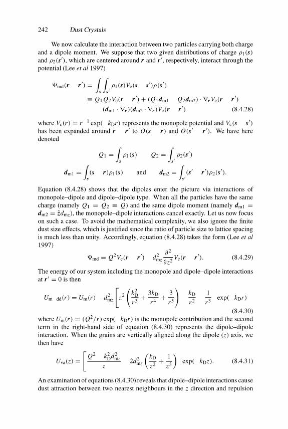
242 Dust Crystals
We now calculate the interaction between two particles carrying both chargeand a dipole moment. We suppose that two given distributions of charge ρ1(s)and ρ2(s′), which are centered around r and r ′, respectively, interact through thepotential (Lee et al 1997)
#md(r − r ′) =∫
s
∫s′ρ1(s)Vc(s − s′)ρ(s′)
≡ Q1 Q2Vc(r − r ′)+ (Q1dm1 − Q2dm2) · ∇r Vc(r − r ′)− (dm1 · ∇r )(dm2 · ∇r )Vc(r − r ′) (8.4.28)
where Vc(r) = r−1 exp(−kDr) represents the monopole potential and Vc(s − s′)has been expanded around r − r ′ to O(s − r) and O(s′ − r ′). We have heredenoted
Q1 =∫
sρ1(s) Q2 =
∫s′ρ2(s′)
dm1 =∫
s(s − r)ρ1(s) and dm2 =
∫s′(s′ − r ′)ρ2(s′).
Equation (8.4.28) shows that the dipoles enter the picture via interactions ofmonopole–dipole and dipole–dipole type. When all the particles have the samecharge (namely Q1 = Q2 ≡ Q) and the same dipole moment (namely dm1 =dm2 = zdmz), the monopole–dipole interactions cancel exactly. Let us now focuson such a case. To avoid the mathematical complexity, we also ignore the finitedust size effects, which is justified since the ratio of particle size to lattice spacingis much less than unity. Accordingly, equation (8.4.28) takes the form (Lee et al1997)
#md = Q2Vc(r − r ′)− d2mz
∂2
∂z2Vc(r − r ′). (8.4.29)
The energy of our system including the monopole and dipole–dipole interactionsat r ′ = 0 is then
Um−dd(r) = Um(r)− d2mz
[z2
(k2
D
r3 +3kD
r4 + 3
r5
)− kD
r2 −1
r3
]exp(−kDr)
(8.4.30)where Um(r) = (Q2/r) exp(−kDr) is the monopole contribution and the secondterm in the right-hand side of equation (8.4.30) represents the dipole–dipoleinteraction. When the grains are vertically aligned along the dipole (z) axis, wethen have
Uva(z) =[
Q2 − k2Dd2
mz
z− 2d2
mz
(kD
z2+ 1
z3
)]exp(−kDz). (8.4.31)
An examination of equations (8.4.30) reveals that dipole–dipole interactions causedust attraction between two nearest neighbours in the z direction and repulsion

Attractive Forces 243
Figure 8.3. The trajectories of ions which intersect both grain 1 and grain 2 (after Lampeet al 2000).
in the x–y plane. For kDr > 1, which is true when the interparticle distanceis larger than λD, the leading terms (which are proportional to z2k2
D/r3 and(3z2kD− kDr2)/r4) come from screening. That is, the effect of the dipole–dipoleinteraction is enhanced by screening. The attractive dipole–dipole force betweenaligned dipoles plays a very important role (Mohideen et al 1998) in intergraincoupling of dielectric grains whose radius is larger than 50 µm.
8.4.4 Shadowing force
There is a continuous bombardment of the ions and electrons onto the dust grainsurface. The ions that are absorbed by a grain impart their momentum to thegrain. For a single isolated grain in a non-streaming plasma, the ion flow to thegrain is spherically symmetric and thus there is on average no net momentumtransfer from the ions to the grains. But if there are two isolated grains, and ifthe ion trajectories are collisionless, some of the ions flowing to grain 2 from thedirection of grain 1 will be intercepted by grain 1 and never reach grain 2. As aresult, the remaining ions that do reach grain 2 impart a net momentum directedtoward grain 1. This represents an effective attractive force between two isolatedgrains in a plasma due to the shadow of a grain (Tsytovich et al 1996). Theshadowing effect was used by Lesage (1782) at the end of the 18th century toexplain the gravitational attraction, since the net force resulting from this effectgoes as r−2.
The calculation of the shadowing force in a dusty plasma is rathercomplicated because ion trajectories that intercept two grains are strongly curvedby Coulomb interaction with the grains (Lampe et al 2000). We consider twograins located at z = ±a/2 (as shown in figure 8.3). All such trajectories mustcross the z = 0 plane with ρ ≤ rd(1−2eφs/miv
2i )
1/2. To estimate the shadowingforce, we assume that the angular momentum about grain 1 is conserved whenthe ion is to the left of the midplane z = 0 (i.e. −a/2 ≥ z ≤ 0), and the angularmomentum about the grain 2 is conserved when the ion is to the right of themidplane z = 0 (i.e. 0 ≥ z ≤ a/2). This is a very good approximation when
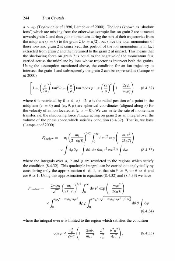
244 Dust Crystals
a > λD (Tsytovich et al 1996, Lampe et al 2000). The ions (known as ‘shadowions’) which are missing from the otherwise isotropic flux on grain 2 are attractedtowards grain 2, and thus gain momentum during the part of their trajectories fromthe midplane (z = 0) to the grain 2 (z = a/2), but since the total momentum ofthese ions and grain 2 is conserved, this portion of the ion momentum is in factextracted from grain 2 and then returned to the grain 2 at impact. This means thatthe shadowing force on grain 2 is equal to the negative of the momentum fluxcarried across the midplane by ions whose trajectories intersect both the grains.Using the assumption mentioned above, the condition for an ion trajectory tointersect the grain 1 and subsequently the grain 2 can be expressed as (Lampe etal 2000)[
1+(
a
2ρ
)2
tan2 θ +(
a
ρ
)tan θ cosϕ
]≤(
rd
ρ
)2(
1− 2eφs
miv2i
)(8.4.32)
where θ is restricted by 0 < θ < π/2, ρ is the radial position of a point in themidplane (z = 0) and (vi, θ, ϕ) are spherical coordinates (aligned along z) forthe velocity of an ion located at (ρ, z = 0). We can write the rate of momentumtransfer, i.e. the shadowing force Fshadow acting on grain 2 as an integral over thevolume of the phase space which satisfies condition (8.4.32). That is, we have(Lampe et al 2000)
Fshadow = − ni
(mi
2πkBTi
)3/2 ∫ ∞
0dv v2 exp
(− miv
2
2kBTi
)
×∫
dρ 2πρ∫
dθ sin θmiv2 cos2 θ
∫dϕ (8.4.33)
where the integrals over ρ, θ and ϕ are restricted to the regions which satisfythe condition (8.4.32). This quadruple integral can be carried out analytically byconsidering only the approximation θ � 1, so that sin θ � θ , tan θ � θ andcos θ � 1. Using this approximation in equations (8.4.32) and (8.4.33) we have
Fshadow = − 2mini√π
(mi
2kBTi
)3/2 ∫ ∞
0dv v4 exp
(− miv
2
2kBTi
)
×∫ rd
√1−2eφs/miv
2
0dρ ρ
∫ (2rd/a)√
1−2eφs/miv2−ρ2/r2
d
0dθ θ
∫dϕ
(8.4.34)
where the integral over ϕ is limited to the region which satisfies the condition
cosϕ ≤ r2d
ρθa
(1− 2eφs
miv2 −ρ2
r2d
− θ2a2
4r2d
). (8.4.35)
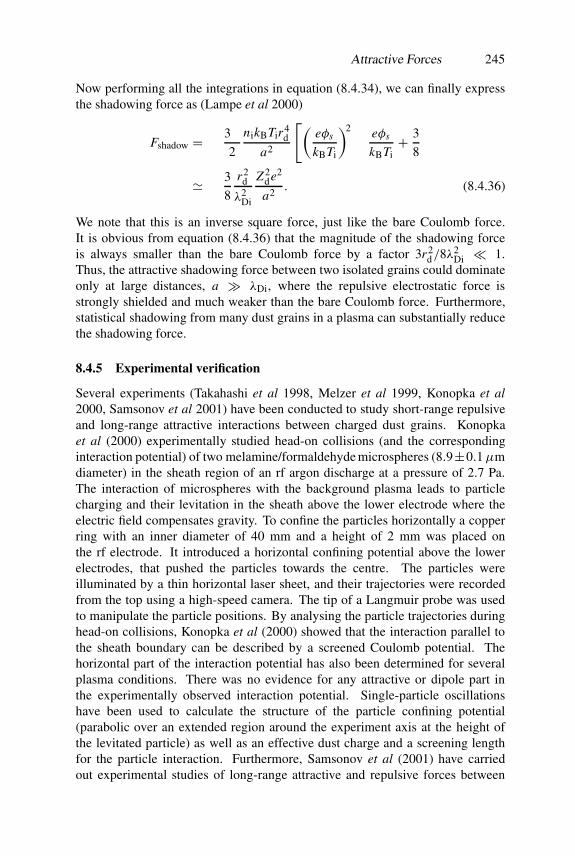
Attractive Forces 245
Now performing all the integrations in equation (8.4.34), we can finally expressthe shadowing force as (Lampe et al 2000)
Fshadow = − 3π
2
nikBTir4d
a2
[(eφs
kBTi
)2
− eφs
kBTi+ 3
8
]
� − 3
8
r2d
λ2Di
Z2de2
a2. (8.4.36)
We note that this is an inverse square force, just like the bare Coulomb force.It is obvious from equation (8.4.36) that the magnitude of the shadowing forceis always smaller than the bare Coulomb force by a factor 3r2
d/8λ2Di � 1.
Thus, the attractive shadowing force between two isolated grains could dominateonly at large distances, a � λDi, where the repulsive electrostatic force isstrongly shielded and much weaker than the bare Coulomb force. Furthermore,statistical shadowing from many dust grains in a plasma can substantially reducethe shadowing force.
8.4.5 Experimental verification
Several experiments (Takahashi et al 1998, Melzer et al 1999, Konopka et al2000, Samsonov et al 2001) have been conducted to study short-range repulsiveand long-range attractive interactions between charged dust grains. Konopkaet al (2000) experimentally studied head-on collisions (and the correspondinginteraction potential) of two melamine/formaldehyde microspheres (8.9±0.1µmdiameter) in the sheath region of an rf argon discharge at a pressure of 2.7 Pa.The interaction of microspheres with the background plasma leads to particlecharging and their levitation in the sheath above the lower electrode where theelectric field compensates gravity. To confine the particles horizontally a copperring with an inner diameter of 40 mm and a height of 2 mm was placed onthe rf electrode. It introduced a horizontal confining potential above the lowerelectrodes, that pushed the particles towards the centre. The particles wereilluminated by a thin horizontal laser sheet, and their trajectories were recordedfrom the top using a high-speed camera. The tip of a Langmuir probe was usedto manipulate the particle positions. By analysing the particle trajectories duringhead-on collisions, Konopka et al (2000) showed that the interaction parallel tothe sheath boundary can be described by a screened Coulomb potential. Thehorizontal part of the interaction potential has also been determined for severalplasma conditions. There was no evidence for any attractive or dipole part inthe experimentally observed interaction potential. Single-particle oscillationshave been used to calculate the structure of the particle confining potential(parabolic over an extended region around the experiment axis at the height ofthe levitated particle) as well as an effective dust charge and a screening lengthfor the particle interaction. Furthermore, Samsonov et al (2001) have carriedout experimental studies of long-range attractive and repulsive forces between
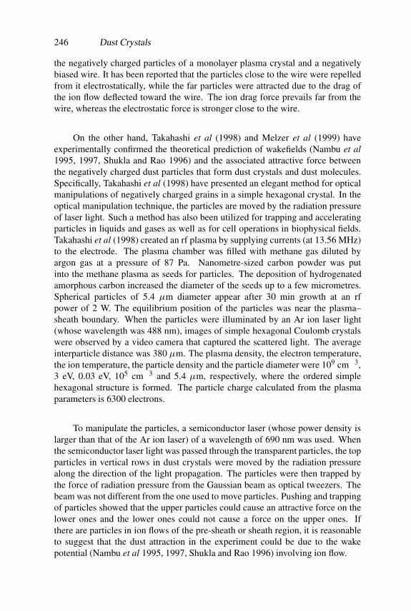
246 Dust Crystals
the negatively charged particles of a monolayer plasma crystal and a negativelybiased wire. It has been reported that the particles close to the wire were repelledfrom it electrostatically, while the far particles were attracted due to the drag ofthe ion flow deflected toward the wire. The ion drag force prevails far from thewire, whereas the electrostatic force is stronger close to the wire.
On the other hand, Takahashi et al (1998) and Melzer et al (1999) haveexperimentally confirmed the theoretical prediction of wakefields (Nambu et al1995, 1997, Shukla and Rao 1996) and the associated attractive force betweenthe negatively charged dust particles that form dust crystals and dust molecules.Specifically, Takahashi et al (1998) have presented an elegant method for opticalmanipulations of negatively charged grains in a simple hexagonal crystal. In theoptical manipulation technique, the particles are moved by the radiation pressureof laser light. Such a method has also been utilized for trapping and acceleratingparticles in liquids and gases as well as for cell operations in biophysical fields.Takahashi et al (1998) created an rf plasma by supplying currents (at 13.56 MHz)to the electrode. The plasma chamber was filled with methane gas diluted byargon gas at a pressure of 87 Pa. Nanometre-sized carbon powder was putinto the methane plasma as seeds for particles. The deposition of hydrogenatedamorphous carbon increased the diameter of the seeds up to a few micrometres.Spherical particles of 5.4 µm diameter appear after 30 min growth at an rfpower of 2 W. The equilibrium position of the particles was near the plasma–sheath boundary. When the particles were illuminated by an Ar ion laser light(whose wavelength was 488 nm), images of simple hexagonal Coulomb crystalswere observed by a video camera that captured the scattered light. The averageinterparticle distance was 380 µm. The plasma density, the electron temperature,the ion temperature, the particle density and the particle diameter were 109 cm−3,3 eV, 0.03 eV, 105 cm−3 and 5.4 µm, respectively, where the ordered simplehexagonal structure is formed. The particle charge calculated from the plasmaparameters is 6300 electrons.
To manipulate the particles, a semiconductor laser (whose power density islarger than that of the Ar ion laser) of a wavelength of 690 nm was used. Whenthe semiconductor laser light was passed through the transparent particles, the topparticles in vertical rows in dust crystals were moved by the radiation pressurealong the direction of the light propagation. The particles were then trapped bythe force of radiation pressure from the Gaussian beam as optical tweezers. Thebeam was not different from the one used to move particles. Pushing and trappingof particles showed that the upper particles could cause an attractive force on thelower ones and the lower ones could not cause a force on the upper ones. Ifthere are particles in ion flows of the pre-sheath or sheath region, it is reasonableto suggest that the dust attraction in the experiment could be due to the wakepotential (Nambu et al 1995, 1997, Shukla and Rao 1996) involving ion flow.
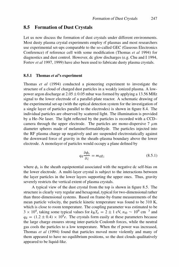
Formation of Dust Crystals 247
8.5 Formation of Dust Crystals
Let us now discuss the formation of dust crystals under different environments.Most dusty plasma crystal experiments employ rf plasmas and most researchersuse experimental set-ups comparable to the so-called GEC (Gaseous ElectronicsConference) rf reference cell with some modification (Thomas et al 1994) fordiagnostics and dust control. However, dc glow discharges (e.g. Chu and I 1994,Fortov et al 1997, 1999) have also been used to fabricate dusty plasma crystals.
8.5.1 Thomas et al’s experiment
Thomas et al (1994) conducted a pioneering experiment to investigate thestructure of a cloud of charged dust particles in a weakly ionized plasma. A low-power argon discharge at 2.05±0.05 mbar was formed by applying a 13.56 MHzsignal to the lower electrode of a parallel-plate reactor. A schematic drawing ofthe experimental set-up (with the optical detection system for the investigation ofa single layer of particles parallel to the electrodes) is shown in figure 8.4. Theindividual particles are observed by scattered light. The illumination is providedby a He–Ne laser. The light reflected by the particles is recorded with a CCD–camera through the upper electrode. The particles are mono-dispersive 7 µmdiameter spheres made of melamine/formaldehyde. The particles injected intothe RF plasma charge up negatively and are suspended electrostatically againstthe downward force of gravity in the sheath–plasma boundary above the lowerelectrode. A monolayer of particles would occupy a plane defined by
−qd∂φs
∂z= mdgz (8.5.1)
where φs is the sheath equipotential associated with the negative dc self-bias onthe lower electrode. A multi-layer crystal is subject to the interactions betweenthe layer particles in the lower layers supporting the upper ones. Thus, gravityseverely restricts the vertical extent of plasma crystals.
A typical view of the dust crystal from the top is shown in figure 8.5. Thestructure is clearly very regular and hexagonal, typical for two-dimensional ratherthan three-dimensional systems. Based on frame-by-frame measurements of themean particle velocity, the particle kinetic temperature was found to be 310 K,which is close to room temperature. The coupling parameter was estimated to be3 × 104, taking some typical values for kBTe = 2 ± 1 eV, ni0 ∼ 109 cm−3 andqd = (1.2 ± 0.4) × 104e. The crystals form easily at these parameters becausethe large charge ensures strong inter-particle Coulomb forces, while the neutralgas cools the particles to a low temperature. When the rf power was increased,Thomas et al (1994) found that particles moved more violently and many ofthem appeared to have no equilibrium positions, so the dust clouds qualitativelyappeared to be liquid-like.
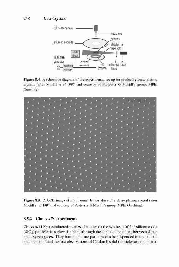
248 Dust Crystals
Figure 8.4. A schematic diagram of the experimental set-up for producing dusty plasmacrystals (after Morfill et al 1997 and courtesy of Professor G Morfill’s group, MPE,Garching).
Figure 8.5. A CCD image of a horizontal lattice plane of a dusty plasma crystal (afterMorfill et al 1997 and courtesy of Professor G Morfill’s group, MPE, Garching).
8.5.2 Chu et al’s experiments
Chu et al (1994) conducted a series of studies on the synthesis of fine silicon oxide(SiO2) particles in a glow discharge through the chemical reactions between silaneand oxygen gases. They found that fine particles can be suspended in the plasmaand demonstrated the first observations of Coulomb solid (particles are not mono-
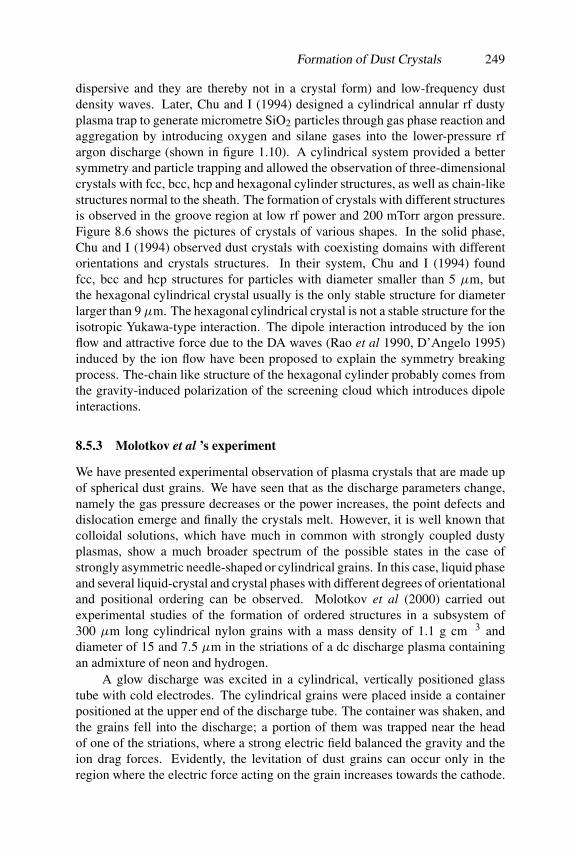
Formation of Dust Crystals 249
dispersive and they are thereby not in a crystal form) and low-frequency dustdensity waves. Later, Chu and I (1994) designed a cylindrical annular rf dustyplasma trap to generate micrometre SiO2 particles through gas phase reaction andaggregation by introducing oxygen and silane gases into the lower-pressure rfargon discharge (shown in figure 1.10). A cylindrical system provided a bettersymmetry and particle trapping and allowed the observation of three-dimensionalcrystals with fcc, bcc, hcp and hexagonal cylinder structures, as well as chain-likestructures normal to the sheath. The formation of crystals with different structuresis observed in the groove region at low rf power and 200 mTorr argon pressure.Figure 8.6 shows the pictures of crystals of various shapes. In the solid phase,Chu and I (1994) observed dust crystals with coexisting domains with differentorientations and crystals structures. In their system, Chu and I (1994) foundfcc, bcc and hcp structures for particles with diameter smaller than 5 µm, butthe hexagonal cylindrical crystal usually is the only stable structure for diameterlarger than 9 µm. The hexagonal cylindrical crystal is not a stable structure for theisotropic Yukawa-type interaction. The dipole interaction introduced by the ionflow and attractive force due to the DA waves (Rao et al 1990, D’Angelo 1995)induced by the ion flow have been proposed to explain the symmetry breakingprocess. The-chain like structure of the hexagonal cylinder probably comes fromthe gravity-induced polarization of the screening cloud which introduces dipoleinteractions.
8.5.3 Molotkov et al ’s experiment
We have presented experimental observation of plasma crystals that are made upof spherical dust grains. We have seen that as the discharge parameters change,namely the gas pressure decreases or the power increases, the point defects anddislocation emerge and finally the crystals melt. However, it is well known thatcolloidal solutions, which have much in common with strongly coupled dustyplasmas, show a much broader spectrum of the possible states in the case ofstrongly asymmetric needle-shaped or cylindrical grains. In this case, liquid phaseand several liquid-crystal and crystal phases with different degrees of orientationaland positional ordering can be observed. Molotkov et al (2000) carried outexperimental studies of the formation of ordered structures in a subsystem of300 µm long cylindrical nylon grains with a mass density of 1.1 g cm−3 anddiameter of 15 and 7.5 µm in the striations of a dc discharge plasma containingan admixture of neon and hydrogen.
A glow discharge was excited in a cylindrical, vertically positioned glasstube with cold electrodes. The cylindrical grains were placed inside a containerpositioned at the upper end of the discharge tube. The container was shaken, andthe grains fell into the discharge; a portion of them was trapped near the headof one of the striations, where a strong electric field balanced the gravity and theion drag forces. Evidently, the levitation of dust grains can occur only in theregion where the electric force acting on the grain increases towards the cathode.

250 Dust Crystals
Figure 8.6. Micrographs and sketches of the different crystal structures: (a) hexagonal, (b)bcc and (c) fcc. The central column corresponds to the structures in the micrographs. Thegraded areas in the sketches are normal to the optical axis. The bars correspond to 0.2 mm(after Chu and I 1994).
Figure 8.7 is the image of the ordered structure of the heavier cylindrical grains(15 µm in diameter) at high gas pressure (0.9 Torr). All the particles lie in theplane perpendicular to the discharge axis and are oriented in a certain direction.At small pressures (∼0.1 Torr), in the lower part of the structures, Molotkov etal (2000) observed oscillations with a wavelength of ∼1 mm and a frequency of20–50 Hz. It was noted that for elongated cylindrical grains with l/2rd � 1, thecharge-to-mass ratio is larger than for a spherical grain with the same mass, wherel is the length of the grain. The charge of a cylindrical grain is (Molotkov et al2000)
qd = Clφd (8.5.2)
where
Cl = l
2ln
(l
rd
). (8.5.3)
For a floating surface potential φd = 30 V, l = 300 µm, 2rd = 15 µm, we haveqd = 7.7 × 10⁵e. Then, in order to balance the gravity acting on a nylon grain
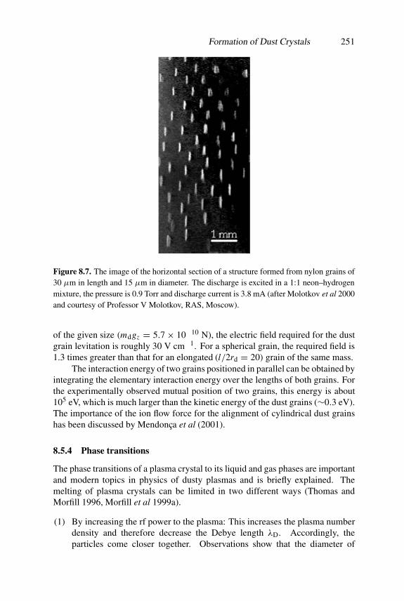
Formation of Dust Crystals 251
Figure 8.7. The image of the horizontal section of a structure formed from nylon grains of30 µm in length and 15 µm in diameter. The discharge is excited in a 1:1 neon–hydrogenmixture, the pressure is 0.9 Torr and discharge current is 3.8 mA (after Molotkov et al 2000and courtesy of Professor V Molotkov, RAS, Moscow).
of the given size (mdgz = 5.7× 10⁻¹⁰ N), the electric field required for the dustgrain levitation is roughly 30 V cm−1. For a spherical grain, the required field is1.3 times greater than that for an elongated (l/2rd = 20) grain of the same mass.
The interaction energy of two grains positioned in parallel can be obtained byintegrating the elementary interaction energy over the lengths of both grains. Forthe experimentally observed mutual position of two grains, this energy is about105 eV, which is much larger than the kinetic energy of the dust grains (∼0.3 eV).The importance of the ion flow force for the alignment of cylindrical dust grainshas been discussed by Mendonca et al (2001).
8.5.4 Phase transitions
The phase transitions of a plasma crystal to its liquid and gas phases are importantand modern topics in physics of dusty plasmas and is briefly explained. Themelting of plasma crystals can be limited in two different ways (Thomas andMorfill 1996, Morfill et al 1999a).
(1) By increasing the rf power to the plasma: This increases the plasma numberdensity and therefore decrease the Debye length λD. Accordingly, theparticles come closer together. Observations show that the diameter of
252 Dust Crystals
the dust cloud shrinks (the number of particles remains constant) and themobility of the particle increases. This could be due to the change in theelectric potential distribution between the electrodes or the increase of theion flow to the electrodes due to the increase of the dc self-bias, or both.
(2) By decreasing the neutral gas pressure: This, in turn, leads to an adjustmentof the plasma parameters and correspondingly the experimental parametersthat determine the value of �d. The pressure variation provides an easy wayto control the plasma conditions through the melting phase transitions.
The melting experiment, as conducted by Thomas and Morfill (1996), startsfrom the well-established crystalline state at 0.42 mbar pressure. Transitionsare followed by continuous lowering of the gas pressure. Both structuraland dynamical properties of the plasma crystal are determined. By analysingtranslational and bond orientational correlation functions, random and systematicparticle motions, self-diffusion, viscosity and interaction cross sections, thefollowing states have been identified during the melting transition.
• Crystalline: This is characterized by a hexagonal horizontal lattice structureand a vertical alignment.
• Flow and floe: This is characterized by the coexistence of islands of orderedcrystalline structure (floes) and systematic directed particle motion (flows).Translational and orientational order have decreased significantly.
• Vibrational: This is characterized by a return to a more orientationallyordered structure and diminishing flow regions. Vibrational amplitudes,thermal energy and vertical migration of particles increase. The translationalorder continues to decrease.
• Disordered: This is characterized by collisions, complete vertical andhorizontal migration. At this stage there is no discernible translational ororientational order: the thermal energy increases to approximately 200 timesthe room temperature, and the Coulomb coupling parameter is of the orderof unity or less.
The lattice structure of a crystal is usually characterized by two quantities—the ‘pair correlation function’, which describes the translational order from onelattice plane to the next, etc and the ‘bond correlation function’, which describesthe orientational order of the crystalline structure around a given origin. Thepair correlation function for the crystalline, liquid and disordered states usuallyshows many sharp peaks corresponding to the various lattice plane locations ina hexagonal lattice and demonstrates the long-range order in the system. Thebond correlation function tests the sixfold symmetry in bond angles to the nearestneighbours (for a hexagonal lattice).

Mach Cones 253
Figure 8.8. A sketch of a Mach cone produced by a supersonic disturbance moving tothe left. The cones are a superposition of spherical (or circular in two dimensions) wavesgenerated by the moving disturbance. The semivertex angle θ is the angle between thecone axis and the wave front (after Samsonov et al 2000).
8.6 Mach Cones
It is well known that an object moving with supersonic speed in a dispersivemedium creates a pressure disturbance that is not felt upstream from the object.The cone that confines the disturbance is called a Mach cone. The latter iswell known in gas dynamics. They are produced, for example, by bullets andsupersonic jet planes. If the perturbing object moves straight at a constant velocityU , it creates expanding waves that are circular in two dimensions and sphericalin three dimensions. The superposition of these waves forms a cone, which isdisplayed in figure 8.8. The Mach angle θ , defined as a semivertex angle of thecone, is determined by the geometry as
θ = sin−1(
1
M
)(8.6.1)
where M = U/CA is the Mach number of the supersonic object and CA is theacoustic (sound) speed in the undisturbed medium.
Mach cones are also known to occur in solid matter (Cheng et al 1994). Inan elastic medium surrounding a fluid-filled borehole, spontaneously launchedsurface waves propagating along the fluid–solid boundary excite P and S wavespropagating into the bulk solid. The interference between P and S waves formsMach cones. The wavefront of the surface wave acts as the supersonic object asits speed is typically higher than the P and S waves.
Ship waves have an appearance similar to Mach cones. The latter are alsoknown as the ‘Kelvin wedge’ that forms behind a ship in deep water. Here amoving point-like disturbance generates either gravity or capillary waves on thefluid surface. These deep water strongly dispersive surface waves (Crapper 1984)are responsible for multiple Mach cone structures.
Besides the above-mentioned Mach cones on human scales, Mach cones alsooccur on astronomical scales (e.g. the Earth’s magnetotail formed by interactionwith the solar wind) and microscopic scales (e.g. Cherenkov radiation created by
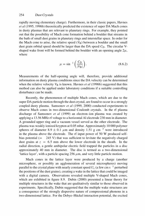
254 Dust Crystals
rapidly moving elementary charge). Furthermore, in their classic papers, Havneset al (1995, 1996b) theoretically predicted the existence of super DA Mach conesin dusty plasmas that are relevant to planetary rings. For example, they pointedout that the possibility of Mach cone formation behind a boulder that streams inthe bath of small dust grains in planetary rings and interstellar space. In order forthe Mach cone to arise, the relative speed (VB) between a boulder and the smalldust grain orbital speed should be larger than the DA speed CD. The circular V-shaped wake front will be formed behind the boulder with an opening angle 2µ,where
µ = sin−1(
CD
|VB|). (8.6.2)
Measurements of the half-opening angle will, therefore, provide additionalinformation on dusty plasma conditions since the DA velocity can be determinedwhen the relative velocity VB is known. Havnes et al (1996b) suggested that thismethod can also be applied under laboratory conditions if a suitable controllingdisturbance can be made.
Recently, the phenomenon of multiple Mach cones, which are due to thesuper DA particle motion through the dust crystal, are found to occur in a stronglycoupled dusty plasma. Samsonov et al (1999, 2000) conducted experiments toobserve Mach cones in two-dimensional Coulomb crystals. In the rf plasmadischarge of Samsonov et al (1999) an electron–ion plasma was created byapplying a 13.56 MHz rf voltage to a horizontal Al electrode 230 mm in diameter.A grounded upper ring and a vacuum vessel served as the other electrode. Theplasma was weakly ionized krypton at 0.05 mbar. Approximately 10 000 polymerspheres of diameter 8.9 ± 0.1 µm and density 1.51 g cm−3 were introducedin the plasma above the electrode. The rf input power of 50 W produced self-bias potential (= −245 V) that was sufficient to levitate the negatively chargeddust grains at z = 6.5 mm above the lower electrode in the sheath. In theradial direction, a gentle ambipolar electric field trapped the particles in a discapproximately 40 mm in diameter. The disc is termed as a two-dimensional‘lattice layer’, with a particle spacing 256 µm, and very little particle motion.
Mach cones in the lattice layer were produced by a charge (anothermicrosphere, or possibly an agglomeration of several microspheres) movingparallel to the crystal plane with nearly constant speed Uc (a few cm s−1 perturbedthe positions of the dust grains), creating a wake in the lattice that could be imagedwith a digital camera. Observations revealed multiple V-shaped Mach cones,which are exhibited in figure 8.9. Dubin (2000) presented a linear theory formultiple structures in the wake that are qualitatively similar to those observed inexperiments. Specifically, Dubin suggested that the multiple wake structures area consequence of the strongly dispersive nature of compressional phonons in atwo-dimensional lattice. For the Debye–Huckel interaction potential, the excited

Particle Dynamics: Microgravity Experiment 255
Figure 8.9. Experimentally observed multiple Mach cones (after Samsonov et al 1999 andcourtesy of D Samsonov, MPE, Garching).
waves have the dispersion relation (Dubin 2000)
ω2(k) = 2πnDq2d0
md
k
(1+ k2λ2D)
1/2(8.6.3)
which satisfy the Mach condition ω/k = Cp = Uc sin θc. Here nD is thedensity per unit area of the dust. For k2λ2
D � 1 equation (8.6.3) takes the formω2 = (2πnDq2
d0/md)k, which is identical to that for deep water surface gravitywaves with 2πnDq2
d0/md taking the role of gravity. However, equation (8.6.3)exhibits that the phonon phase speed strongly depends on the wavevector k,namely Vp = Vp(k). Hence different excited waves would travel at differentpropagation angle θc(k). Phase mixing of the various excited dispersive wavescauses constructive and destructive interference. As a result, along a line definedby some opening angle ψc, there are specific wavenumbers k = k0(ψc) that aredominant. In general, the propagation angle θc for these wavenumbers is notequal to ψc. These wavenumbers form the observed multiple wakes. The long-wavelength features of the wake in a two dimensional Coulomb crystal shouldresemble the Kelvin wedge behind a moving ship in deep water.
8.7 Particle Dynamics: Microgravity Experiment
The parabolic flight campaigns and sounding rocket experiments as well asdc glow discharges and UV-induced dusty plasmas provide the possibility ofinvestigating the dynamics and trajectories of dust particles under microgravityconditions. The results of parabolic flights (short-time µg-flights of 25 s each)are summarized by Thomas et al (2001). The experiments use a symmetrically

256 Dust Crystals
Figure 8.10. The particle trajectories grey-coded from the beginning of the trajectory to itsend from the TEXUS 35 microgravity experiment (after Thomas et al 2001 and courtesyof Dr H Thomas, MPE, Garching).
Figure 8.11. The original image of the distribution of the particles of different sizes (3.4and 1.9 µm) in the plasma chamber (after Thomas et al 2001 and courtesy of Dr H Thomas,MPE, Garching).
driven rf discharge containing inert gases (argon, krypton and xenon). Particlesof four different sizes (1.2, 1.9, 3.4 and 6.9 µm) were injected into the plasmathrough a specially designed dispenser incorporated in each of the electrodes.They are charged in a few tens of microseconds and then interact with each otherand with the global electric field. A typical distribution of particles is shownin figure 8.10, which shows the particle motion between the two rf electrodes.

Particle Dynamics: Microgravity Experiment 257
The centre of the system is particle free (Morfill et al 1999b). In the absenceof gravity, charged dust microspheres are usually embedded in the main plasma,where the major bulk forces are the electric force (qd E0), the thermophoreticforce (FT), the ion drag force (Fdi), as well as the neutral density gradient (Fgr)and drag (Fdn) forces. The forces FT and Fdi are directed outwards, while qd E0and Fgr are directed into the main plasma. The frictional force slows the particlesdown. The ratio between the outward and inward forces determine the positionof the particulates. For particles in the micron size range, it is possible, undermicrogravity conditions, to adjust the system largely force free provided that FTand Fdi are held small. For the conditions of figure 8.10, the outward force farexceeds the inward force, and consequently, there appears a void in the centre(Morfill et al 1999b). The void seems to be created by the thermophoretic forcerather than by the ion drag force; the latter is at least one order of magnitudesmaller than FT under microgravity conditions. The behaviour of a mixture ofparticles of two different sizes was investigated during the parabolic flights. Undermicrogravity conditions, particle clouds of two different particle sizes becomeseparated vertically due to their different charge-to-mass ratios. Only for thosecases where the charge-to-mass ratio is identical for particles of different sizes, itis possible to obtain levitation at the same height. Under microgravity the massof the particles no longer matters but the size of the particles still has to be takeninto consideration, because the electric force acting on the microparticles dependson their size (namely qd E0 ∝ rd). It is obvious that the different particle sizesseparate. The smaller particles are found closer to the centre of the discharge, thelarger ones further outwards from the centre where the electric field is stronger.The two microparticle clouds are separated by a sharp boundary, as shown infigure 8.11. It should be stressed that the microgravity experiments are beingcarried out on board the International Space Station (ISS) under microgravityconditions. We hope that the forthcoming ISS data will reveal new aspectsof numerous collective processes caused by charged macroparticles in a dustyplasma.

References
Alexandrov A F, Bogdankevich L S and Rukhadze A A 1984 Principles of PlasmaElectrodynamics (Berlin: Springer)
Alfven H 1954 On the Origin of the Solar System (Oxford: Clarendon)Allen J E 1992 Phys. Scripta 45 497Annaratone B M et al 2001 Phys. Rev. E 63 036406Avinash K and Shukla P K 1994 Phys. Lett. A 189 470Backhouse T W 1885 Meteorol. Mag. 20 133Baines M J, Williams I P and Asebiomo A S 1965 Mon. Not. R. Astron. Soc. 130 63Barkan A, D’Angelo N and Merlino R L 1994 Phys. Rev. Lett. 73 3093Barkan A, Merlino R L and D’Angelo N 1995a Phys. Plasmas 2 3563Barkan A, D’Angelo N and Merlino R L 1995b Planet. Space Sci. 43 905——1996 Planet. Space Sci. 44 239Barnes M S, Keller J H, Foster J C, O’Neill J A and Coultas D K 1992 Phys. Rev. Lett. 68
313Benkadda S, Tsytovich V N and Vegra A 1995 Commun. Plasma Phys. Control. Fusion 16
321Bernhardt P A, Ganguli G, Kelley M C and Swartz W E 1995 J. Geophys. Res. 100 23811Bharuthram R and Shukla P K 1992a Planet. Space Sci. 40 973——1992b Planet. Space Sci. 40 647Birk G T, Kopp A and Shukla P K 1996 Phys. Plasmas 3 3564Bittencourt J A 1986 Fundamentals of Plasma Physics (Oxford: Pergamon)Bliokh P, Sinitsin V and Yaroshenko V 1995 Dusty and Self-Gravitational Plasmas in
Space (Dordrecht: Kluwer Academic)Boeuf J P and Punset C 1999 Dusty Plasmas: Physics, Chemistry and Technological
Impacts in Plasma Processing ed A Bouchoule (New York: Wiley) pp 1–76Bouchoule A 1999 Dusty Plasmas: Physics, Chemistry and Technical Impacts in Plasma
Processing ed A Bouchoule (New York: Wiley) pp 305–96Brattli A, Havnes O and Melandsø F 1997 J. Plasma Phys. 58 691Charney J G 1947 Geophys. Publ. 17 17Chen F F 1965 Plasma Diagnostic Techniques ed R H Huddlestone and S L Leonard (New
York: Academic) ch 4Chen F F 1974 Introduction to Plasma Physics (New York: Plenum)——1995 Phys. Plasmas 2 2164Chen L, Langdon A B and Lieberman M A 1973 J. Plasma Phys. 9 311Chen X and Tao X 1992 Plasma Chem. Plasma Proc. 12 345Cheng N, Zhu Z, Cheng C and Toksoz M 1994 Geophysical Prospecting 42 303
258
References 259
Cho J Y N and Kelley M C 1993 Rev. Geophys. 31 243Chow V W, Mendis D A and Rosenberg M 1993 J. Geophys. Res. 98 19 065Chow V W and Rosenberg M 1995 Planet. Space Sci. 43 613Chu J H, Du J B and I L 1994 J. Phys. D: Appl. Phys. 27 296Chu J H and I L 1994 Phys. Rev. Lett. 72 4009Crapper G 1984 Introduction to Water Waves (Chichester: Harwood)D’Angelo N 1965 Phys. Fluids 8 1748——1990 Planet Space Sci. 38 1143——1995 J. Phys. D: Appl. Phys. 28 1009——1997 Phys. Plasmas 4 3422——1998 Phys. Plasmas 5 3155D’Angelo N, Barkan A and Merlino R L 1996 The Physics of Dusty Plasmas ed
P K Shukla, D A Mendis and V W Chow (Singapore: World Scientific) pp 93–101D’Angelo N and Song B 1990 Planet. Space Sci. 38 1671de Angelis U 1992 Phys. Scripta 45 465de Angelis U and Forlani A 1998 Phys. Plasmas 5 3068de Gennes P G 1966 Superconductivity of Metals and Alloys (New York: Benjamin)Daugherty J E, Porteous R K and Graves D B 1993 J. Appl. Phys. 73 1617Daugherty J E and Graves D B 1995 J. Appl. Phys. 78 2279Draine B T and Salpeter E E 1979 Astrophys. J. 231 77Dubin D H E 2000 Phys. Plasmas 7 3895Elskens Y, Resendes D P and Mendonca J T 1997 Phys. Plasmas 4 4210Epstein P S 1924 Phys. Rev. 23 710Farokhi B, Shukla P K, Tsintsadze N L and Tskhakaya D D 1999 Phys. Lett. A 264 318——2000 Phys. Plasmas 7 814Feuerbacher B, Willis R F and Fitton B 1973 Astrophys. J. 181 102Fortov V E, Kharpak A G, Kharpak S A, Molotkov V I, Nefedov A P, Petrov O F and
Torchinsky V M 2000 Phys. Plasmas 7 1374Fortov V E, Molotkov V I, Nefedov A P and Petrov O F 1999 Phys. Plasmas 6 1759Fortov V E, Nefedov A P, Torchinsky V M, Molotkov V I, Petrov O F, Samarian A A,
Lipaev A M and Khrapak A G 1997 Phys. Lett. A 229 317Fried B D and Conte S D 1961 The Plasma Dispersion Functions (New York: Academic)Gallagher A 2000 Phys. Rev. E 62 2690Garscadden A, Ganguly B N, Haaland P D and Williams J 1994 Plasma Sources Sci.
Technol. 3 239Glanz J 1994 Science 264 28Goertz C K 1989 Rev. Geophys. 27 271Goertz C K and Morfill G E 1983 Icarus 53 219Gradsteyn I S and Ryzhik I M 2000 Tables of Integrals, Series and Products 6th edn (New
York: Academic) translated from the Russian by Scripta TechnikaGuerra R and Mendonca J T 2000 Phys. Rev. E 62 1190Haaland P 1990 J. Chem. Phys. 93 4066Hamaguchi S and Farouki R T 1994 Phys. Rev. E 49 4430Harwit M 1988 Astrophysical Concepts (New York: Springer) p 405Hasegawa A 1975 Plasma Instabilities and Nonlinear Effects (Berlin: Springer)——1985 Adv. Phys. 34 1Hasegawa A and Mima K 1978 Phys. Fluids 21 87Havnes O 1988 Astron. Astrophys. 193 309

260 References
Havnes O, Aslaksen T K and Melandsø F 1990 J. Geophys. Res. 95 6581Havnes O, Goertz C K, Morfill G E, Grun E and Ip W 1987 J. Geophys. Res. 92 2281Havnes O, Li F, Aslaksen T, Hartquist T W, Li F, Melandsø F, Morfill G E and Nitter T
1995 J. Geophys. Res. 100 1731Havnes O, Li F, Melandsø F, Aslaksen T, Hartquist T W, Morfill G E, Nitter T and
Tsytovich V N 1996b J. Vac. Sci. Technol. A 14 525Havnes O, Nitter T, Tsytovich V N, Morfill G E and Hartquist T W 1994 Plasma Sources
Sci. Technol. 3 448Havnes O, Trøim J, Blix T, Mortensen W, Næsheim L I, Thrane E and Tønnesen 1996a J.
Geophys. Res. 101 10 839Hayashi H and Tachibana K 1994 Japan. J. Appl. Phys. 33 804Hill J R and Mendis D A 1981a Moon and Planets 24 431——1981b Can. J. Phys. 59 897Hollenstein C 2000 Plasma Phys. Control. Fusion 42 R93Homann A, Melzer A, Peters S and Piel A 1997 Phys. Rev. E 56 7138Hopkins M B and Lawler J F 2000 Plasma Phys. Control. Fusion 42 B189Horanyi M and Goertz C K 1990 Astrophys. J. 361 105Howard J E, Dullin H R and Horanyi M 2000 Phys. Rev. Lett. 84 3244Howard J E, Horanyi M and Stewart G R 1999 Phys. Rev. Lett. 83 3993Ichimaru S 1973 Basic Principles of Plasma Physics: A Statistical Approach (London:
Benjamin)——1982 Rev. Mod. Phys. 54 1017Ichimaru S, Iyetomi H and Tanaka S 1987 Phys. Rep. 149 91Iizuka S, Saeki K, Sato N and Hatta Y 1985 J. Phys. Soc. Japan 54 146Ikezi H 1986 Phys. Fluids 29 1764Ishihara O 1998 Phys. Scripta T 75 79Ishihara O and Sato N 2001 IEEE Trans. Plasma Sci. 29 000Ivlev A V, Konopka U and Morfill G E 2000a Phys. Rev. E 62 2739Ivlev A V, Suterlin R, Steinberg V, Zuzic M and Morfill G E 2000b Phys. Rev. Lett. 85
4060Jana M R, Sen A and Kaw P K 1993 Phys. Rev. E 48 3930Jonker J H 1952 Phillips Res. Rep. 7 1Karpman V I 1975 Nonlinear Waves in Dispersive Media (Oxford: Pergamon)Kaw P K and Sen A 1998 Phys. Plasmas 5 3552Kim K Y 1983 Phys. Lett. A 97 45Kim K and Kim D 2000 J. Appl. Phys. 87 269Kittel C 1956 Introduction to Solid State Physics (New York: Wiley) ch 11Klimontovich Y L 1982 Kinetic Theory of Nonideal Gases and Nonideal Plasmas (New
York: Pergamon)Knudsen M 1991 Ann. Phys. 34 593Konopka U, Morfill G E and Ratke L 2000 Phys. Rev. Lett. 84 891Kortshagen U and Bhandarkar U 1999 Phys. Rev. E 60 887Krall N A and Trivelpiece A W 1973 Principles of Plasma Physics (New York: McGraw-
Hill)Kushner M 1988 J. Appl. Phys. 63 2532.Laframboise J G and Parker L W 1973 Phys. Fluids 16 629Lampe M, Joyce G, Ganguli G and Gavrishchaka 2000 Phys. Plasmas 7 3851Landau L D and Lifshitz E M 1960 Mechanics (Oxford: Pergamon)

References 261
——1971 The Classical Theory of Fields (Oxford: Pergamon)——1989 Statistical Physics (Oxford: Pergamon)Lapenta G 1999 Phys. Plasmas 6 1442Larichev V D and Reznik G M 1976 Dokl. Akad. Nauk. USSR 231 1077Laroussi M, Sayler G S, Glascock B B, McCurdy B, Pearce M E, Bright N G and Malott
C M 1999 IEEE. Trans. Plasma Sci. 27 34Lee H C, Chen D Y and Rosenstein B 1997 Phys. Rev. E 56 4596Lesage G L 1782 Nouveaux Memoires de l‘Academie Royales des Sciences et des Belles—
Letters (Berlin: Springer) p 404Liu J and Horton W 1986 J. Plasma Phys. 36 1Liu J, Juan W, Hsu J, Huang Z and I L 1999 Plasma Phys. Control. Fusion 41 A47Luo Q Z, D’Angelo N and Merlino R L 1999 Phys. Plasmas 6 3455——2000 Phys. Plasmas 7 2370——2001 Phys. Plasmas 8 31Ma J X and Liu J 1997 Phys. Plasmas 4 253Ma J X and Yu M Y 1994a Phys. Rev. E 50 R2431——1994b Phys. Plasmas 1 3520——1995 Phys. Plasmas 2 1343Madigan M, Martinko J M and Parker J 1997 Biology of Microorganisms 8th edn
(Englewood Cliffs, NJ: Prentice-Hall)Mahmoodi J, Shukla P K, Tsintsadze N L and Tskhakaya D D 2000 Phys. Rev. Lett. 84
2626Mamun A A 1998 Phys. Scripta 57 258Mamun A A 1999 Astrophys. Space Sci. 268 443Mamun A A, Cairns R A and Shukla P K 1996a Phys. Plasmas 3 702——1996b Phys. Plasmas 3 2610Mamun A A and Shukla P K 2000 Phys. Plasmas 7 3499Maxon S and Viecelli J 1974 Phys. Rev. Lett. 32 4Melandsø F 1996 Phys. Plasmas 3 3890Melandsø F, Aslaksen T and Havnes O 1993 Planet. Space Sci. 41 321Melandsø F and Shukla P K 1995 Planet. Space Sci. 43 635Melzer A, Homann A, Piel A and Schweigert I V 1998 in Physics of Dusty Plasmas:
Seventh Workshop ed M Horanyi, S Robertson and B Walch (New York: AmericanInstitute of Physics) pp 167–74
Melzer A, Schweigert I V and Piel A 1999 Phys. Rev. Lett. 83 3194Melzer A, Trottenberg T and Piel A 1994 Phys. Lett. A 191 301Mendis D A 1991 Astrophys. Space Sci. 176 163Mendis D A 1997 Advances in Dusty Plasmas ed P K Shukla, D A Mendis and T Desai
(Singapore: World Scientific) pp 3–19Mendis D A and Axford W I 1974 Rev. Earth Planet Sci. 2 419Mendis D A and Horanyi M 1991 Cometary Plasma Processes ed A J Johnston
(Washington, DC: Geophys. Mongr. No. 6) p 17Mendis D A, Houpis H L F and Hill J R 1982 J. Geophys. Res. 87 3449Mendis D A and Rosenberg M 1994 Ann. Rev. Astron. Astrophys. 32 419Mendis D A, Rosenberg M and Azam F 2000 IEEE. Trans. Plasma Sci. 28 1304Mendonca J T, Shukla P K and Bingham R 2001 Phys. Lett. A 282 288Mendoza-Briceno C A, Russel S M and Mamun A A 2000 Planet. Space Sci. 48 599Merlino R L, Barkan A, Thompson C and D’Angelo N 1998 Phys. Plasmas 5 1607
262 References
Messenger S 2000 Nature 404 968Meuris P 1997 Planet. Space Sci. 45 1171Meyer-Vernet N 1982 Aston. Astrophys. 105 98Mikhailovskii A B 1974 Theory of Plasma Instabilities: Instabilities of a Homogenous
Plasma vol 1 (New York: Consultants Bureau)Miswa T, Ohno N, Asano K, Sawai M, Takamura S and Kaw P K 2001 Phys. Rev. Lett. 86
1219Miyamoto K 1980 Plasma Physics for Nuclear Fusion (Cambridge, MA: MIT)Mohideen U, Rahman H U, Smith M A, Rosenberg M and Mendis D A 1998 Phys. Rev.
Lett. 81 349Molotkov V I, Nefedov A P, Putsyl’nik M Y, Torchinsky V M, Fortov V E, Kharpak A G
and Yoshino K 2000 JETP Lett. 71 102Molotkov V I, Nefedov, Torchinskii V M, Fortov V E and Khrapak A G 1999 Sov. Phys.–
JETP 89 477Montgomery D, Joyce G and Sugihara R 1968 Plasma Phys. 10 681Morfill G E and Thomas H 1996 J. Vac. Sci. Technol. A 14 490Morfill G E, Thomas H M, Konopka U and Zuzic M 1999a Phys. Plasmas 6 1769Morfill G E, Thomas H M, Konopka U, Rothermal H, Zuzic M, Ivlev A and Goree J 1999b
Phys. Rev. Lett. 83 1598Morfill G E, Thomas H M and Zuzic M 1997 Advances in Dusty Plasmas ed P K Shukla,
D A Mendis and T Desai (Singapore: World Scientific) pp 99–142Nakamura Y, Bailung H and Shukla P K 1999 Phys. Rev. Lett. 83 1602Nambu M and Akama H 1985 Phys. Fluids 28 2300Nambu M, Vladimirov S V and Shukla P K 1995 Phys. Lett. A 230 40——1997 Advances in Dusty Plasmas ed P K Shukla, D A Mendis and T Desai (Singapore:
World Scientific) pp 449–52Nayfeh A H and Mook D T 1979 Nonlinear Oscillations (New York: Wiley)Neufeld J and Ritchie R H 1955 Phys. Rev. 98 1635Nitter T 1996 Plasma Sources Sci. Technol. 5 93Northrop T G 1992 Phys. Scripta 45 17Northrop T G and Birmingham T J 1990 Planet. Space Sci. 38 319Nunomura S, Miswa S, Ohno N and Takamura S 1999 Phys. Rev. Lett. 83 1970Ockert M E, Cuzzi J N, Porco C C and Johnson T V 1987 J. Geophys. Res. 92 14 696Okuda H and Dawson J M 1973 Phys. Fluids 16 408Opik E J 1956 Irish Astron. J. 4 84Pandey B P, Avinash K and Dwivedi C B 1994 Phys. Rev. E 49 5599Perrin J and Hollenstein C 1999 Dusty Plasmas: Physics, Chemistry and Technical Impacts
in Plasma Processing ed A Bouchoule (New York: Wiley) pp 77–180Perrin J, Molinas-Mata P and Belenguer P 1994 J. Phys. D: Appl. Phys. 27 2499Pieper J B and Goree J 1996 Phys. Rev. Lett. 77 3137Pokhotelov O A, Onishchenko O G, Shukla P K and Stenflo L 1999 J. Geophys. Res. 104
19 797Popel S I, Yu M Y and Tsytovich V N 1996 Phys. Plasmas 3 4313Prabhuram G and Goree J 1996 Phys. Plasmas 3 1212Rahman H U, Mohideen U, Smith M A, Rosenberg M and Mendis D A 2001 Phys. Scripta
T 89 186Rao N N 1993 J. Plasma Phys. 49 375Rao N N and Shukla P K 1994 Planet. Space Sci. 42 221
References 263
Rao N N, Shukla P K and Yu M Y 1990 Planet Space Sci. 38 543Resendes D P 2000 Phys. Rev. E 61 793Resendes D P, Mendonca J T and Shukla P K 1998 Phys. Lett. A 239 181Resendes D P and Shukla P K 2001 Phys. Scripta T 89 101Rosenberg M 1993 Planet. Space Sci. 41 229Rosenberg M 1996 J. Vac. Sci. Technol. A 14 631Rosenberg M and Kalman G 1997 Phys. Rev. E 56 7166Rosenberg M and Mendis D A 1992 J. Geophys. Res. 97 773——1995 IEEE Trans. Plasma Sci. 23 177Rosenberg M, Mendis D A and Sheehan D P 1996 IEEE Trans. Plasma Sci. 24 1422——1999 IEEE Trans. Plasma Sci. 27 239Rosenberg M and Shukla P K 1998 Phys. Plasmas 5 3786——2000 J. Geophys. Res. 105 23 135Roth R M, Spears K G and Wong G 1985 Appl. Phys. Lett. 46 253Sagdeev R Z 1966 Reviews of Plasma Physics vol 4, ed M A Leontovich (Consultants
Bureau, New York) p 23Salimullah M and Shukla P K 1999 Phys. Plasmas 6 686Samaryan A A, Chernyshev A V, Nefedov A P, Petrov O F, Mikhailov Y M, Mintsev V B
and Fortov V E 2000 Sov. Phys.–JETP 90 817Samsonov D and Goree J 1999 Phys. Rev. E 59 1047Samsonov D, Goree J, Ma Z W, Bhattacharjee A, Thomas H M and Morfill G E 1999 Phys.
Rev. Lett. 83 3649Samsonov D, Goree J, Thomas H M and Morfill G E 2000 Phys. Rev. E 61 5557Samsonov D, Ivlev A V, Morfill G E and Goree J 2001 Phys. Rev. E 63 025401(R)Sato N, Uchida G, Kaneko T, Shimizu S and Iizuka S 2001 Phys. Plasmas 8 1786Sato N, Uchida G, Ozaki R, Iizuka S and Kamimura T 2000 Frontiers in Dusty Plasmas
ed Y Nakamura, T Yokota and P K Shukla (Singapore: World Scientific) pp 329–36Schamel H 1972 Plasma Phys. 14 905——1975 J. Plasma Phys. 13 129——1986 Phys. Rep. 140 161Schamel H, Das N and Rao N N 2001 Phys. Plasmas 8 671Schmidt M J and Gary S P 1973 J. Geophys. Res. 78 8261Selwyn G S 1993 Japan. J. Appl. Phys. 32 3068Selwyn G S, Singh J and Bennet R S 1989 J. Vac. Sci. Technol. A 7 2758Shukla P K 1992 Phys. Scripta 45 504——1996 The Physics of Dusty Plasmas ed P K Shukla, D A Mendis and V W Chow
(Singapore: World Scientific) pp 107–21——1999 Phys. Lett. A 252 340——2000a Phys. Rev. E 61 7249——2000b Phys. Lett. A 268 100——2000c Phys. Rev. Lett. 84 5328——2000d Phys. Plasmas 7 1044——2001 Phys. Plasmas 8 1791Shukla P K and Mamun A A 2001 IEEE Trans. Plasma Sci. 29 221Shukla P K and Morfill G M 1999 Phys. Scripta T 82 119Shukla P K and Rahman H U 1996 Phys. Plasmas 3 430Shukla P K and Rao N N 1996 Phys. Plasmas 3 1770Shukla P K and Rosenberg M 1999 Phys. Plasmas 6 1038

264 References
Shukla P K and Salimullah 1996 Phys. Plasmas 3 3858Shukla P K and Silin V P 1992 Phys. Scripta 45 508Shukla P K and Stenflo L 1999 Nonlinear MHD Waves and Turbulence ed T Passot and
P L Sulem (Berlin: Springer) pp 1–30——2001a IEEE Trans. Plasma Sci. 29 267——2001b Plasma Phys. Rep. 27 904Shukla P K and Varma R K 1993 Phys. Fluids B 5 236Shukla P K and Verheest F 1999 Astrophys. Space Sci. 262 157Shukla P K, Yu M Y and Bharuthram R 1991 J. Geophys. Res. 96 21343Singh S V and Rao N N 1997 Phys. Lett. A 235 164Slattery W L, Doolen G D and DeWitt H E 1980 Phys. Rev. A 21 2087Smith B A et al 1981 Science 212 163——1982 Science 215 504Sodha M S and Guha S 1971 Advances in Plasma Physics vol 4, ed A Simon and
W B Thompson (New York: Wiley) pp 219–309Spitzer L Jr 1977 Physical Processes in the Interstellar Medium (New York: Wiley)Stenflo L 1981 Phys. Rev. A 23 2730——1985 J. Geophys. Res. 90 5355Stenflo L and Shukla P K 2000 Phys. Plasmas 7 3472Stenflo L, Shukla P K and Yu M Y 2000 Phys. Plasmas 7 2731Stenflo L, Yu M Y and Shukla P K 1973 Phys. Fluids 16 450Sternglass E J 1954 Sci. Pap. 1772 (Pittsburgh, PA: Westinghouse Research Laboratory)Takahashi K, Oishi T, Shimomami K, Hayashi Y and Nishino S 1998 Phys. Rev. E 58 7805Talbot L, Cheng R K, Schefer R W and Willis D R 1980 J. Fluid Mech. 101 737Thomas E Jr and Watson M 2000 Phys. Plasmas 7 3194Thomas G E 1991 Rev. Geophys. 29 553Thomas H, Goldbeck, Hagel T, Ivlev A V, Konopka U, Morfill G E, Rothermel H, Suterlin
and Zuzic M 2001 Phys. Scripta T 89 16Thomas H and Morfill G E 1996 Nature 379 806Thomas H, Morfill G E, Demmel V, Goree J, Feuerbacher B and Mohlmann D 1994 Phys.
Rev. Lett. 73 652Thompson C, Barkan A, Merlino R L and D’Angelo N 1999 IEEE Trans. Plasma Sci. 27
146Tonks L and Langmuir I 1929 Phys. Rev. 33 195Tskhakaya D and Shukla P K 2001 Phys. Lett. A 279 456Tskhakaya D, Shukla P K and Tsintsadze N L 2001 Sov. Phys.–JETP 93 301Tsytovich V N 1997 Sov. Phys.–Usp. 40 53Tsytovich V N and Havnes O 1993 Commun. Plasma Phys. Control. Fusion 15 267Tsytovich V N, Khodataev Y K and Bingham R 1996 Commun. Plasma Phys. Control.
Fusion 17 249Vanossi A, Rasmussen K Ø, Bishop A R, Malomed B A and Bortolani V 2000 Phys. Rev.
E 62 7353Varma R K, Shukla P K and Krishan V 1993 Phys. Rev. E 47 3612Verheest F 2000 Waves in Dusty Plasmas (Dordrecht: Kluwer Academic)Vranjes J, Petrovic D and Shukla P K 2001 Phys. Lett. A 278 231Walch B, Horanyi M and Robertson S 1994 IEEE Trans. Plasma Sci. 22 97Wang L 1999 Commun. Mod. Phys. C: Commun. Plasma Phys. Control. Fusion 1 117Wang X, Bhattacharjee A and Hu S 2001 Phys. Rev. Lett. 86 2569
References 265
Washimi H and Taniuti T 1966 Phys. Rev. Lett. 17 996Weiland J 2000 Collective Modes in Inhomogeneous Plasma (Bristol: IOP Publishing)Whiddington R 1912 Proc. R. Soc. A 86 360Whipple E C 1981 Rep. Prog. Phys. 44 1197Whipple E C, Northrop T G and Mendis D A 1985 J. Geophys. Res. 90 7405Wigner E 1938 Trans. Faraday Soc. 34 678Winske D, Gary S P, Jones M E, Rosenberg M, Mendis D A and Chow V W 1995 Geophys.
Res. Lett. 22 2069Winske D and Jones M E 1994 IEEE Trans. Plasma. Sci. 22 454Winske D and Rosenberg M 1998 IEEE Trans. Plasma Sci. 26 92Winter J 1998 Plasma Phys. Control. Fusion 40 1201——2000 Phys. Plasmas 7 3862Wurden G A, Wurden A J and Gladstone I M 1999 IEEE Trans. Plasma Sci. 27 142Xu W, Song B, Merlino R L and D’Angelo N 1992 Rev. Sci. Instrum. 63 5266Yanagita S 1977 Astrophys. Space Sci. 49 L11Zakharov V E 1972 Sov. Phys.–JETP 35 908
Index
accommodation coefficient, 48, 80,81
acoustic modes, 94agglomeration, 32–34Alfven speed, 120Alfven waves, 122, 127–129Ampere’s law, 121, 130asteroid belt, 9astrophysics, 29attractive forces, 235
Bohm criterion, 28, 63, 64Boltzmann distribution, 5, 114Boltzmann equation, 101bouncing motion, 190boundary effects, 145Buneman instability, 146, 147
Cassini Division, 13cauliflower, 18, 19, 21, 34, 46Chapman–Enskog expression, 80,
81characteristic frequencies, 6charge fluctuation, 60, 62, 64, 95,
100, 102, 104, 105, 208, 235charging equation, 58, 153charging processes, 36, 37, 48, 60charging time, 59circularly polarized waves, 120circumstellar clouds, 8coagulation, 8, 30, 32, 65, 66, 170collection of plasma particles, 37,
58, 69, 152collision impact parameter, 148collision operator, 101
collisional effects, 141colloidal chemistry, 32colloidal crystals, 228, 232comet Hale-Bopp, 12comets, 9complementary error function, 40complex plasma, 2continuity equation, 6, 95, 96, 121,
148, 153convective cells, 119, 124Coulomb collisions, 77Coulomb coupling parameter, 7, 22,
23, 35, 50, 110, 230Coulomb crystals, 35Coulomb drag force, 78Coulomb logarithm, 148crystal physics, 34cylindrical and spherical DAS
waves, 208cylindrical grains, 249, 250, 251
DA shock waves, 213DA wave instability, 166dark spokes, 29, 70, 85dc discharges, 18, 25Debye shielding, 4, 27, 60, 61Debye–Huckel potential, 112, 113,
235DIA shock waves, 214DIA wave instability, 166diamagnetic drift, 224, 225dielectric constant, 102, 236dielectric permittivity, 175
266

Index 267
dielectric susceptibility, 102, 103,117, 139, 234
diffusion coefficient, 92dipole moment, 170, 173, 174, 176,
191, 192, 235, 241dipole vortex, 221, 222, 226dipole–dipole interactions, 241, 242dispersion relation, 95, 97, 99, 111,
114, 122, 125, 127, 139,144, 145, 153, 157, 163,180, 183, 187
dispersive Alfven waves, 127disruption of bacteria, 67double layers, 210, 211drag forces, 76, 148, 151dressed grains, 235drift wave instabilities, 156drift-kinetic Alfven waves, 129dust acoustic (DA) waves, 3, 94,
96–99, 103–106, 108, 109,111, 112, 123, 132, 133,141, 151, 153, 162, 180,236, 237
dust Alfven waves, 122dust charge and current densities,
171dust charge gradient, 151–157dust cloud potential, 51, 52dust correlations, 110, 111dust crystals, 228, 230, 231dust cyclotron waves, 119, 123, 144dust drift wave, 126, 157dust fluid temperature, 200dust grain charge, 50, 53, 54, 74dust inertia, 95dust ion-acoustic (DIA) waves, 3,
94, 96, 97, 100, 104–106,118, 125, 134, 135, 140,145, 181, 187, 236, 237
dust lattice (DL) waves, 113, 114,116, 135, 232
dust lattice solitary waves, 212dust magnetosonic waves, 122dust size distributions, 107, 108
dust whistler, 123, 129, 185dust-acoustic solitary (DAS) waves,
198, 199, 200, 205, 208dusty magnetoplasma, 117, 120,
122dusty plasma device (DPD), 23, 24dusty plasma, 1, 17, 21, 62, 81dynamics of dust grains, 70
Earth’s atmosphere, 15EIC instability, 168electromagnetic force, 71electromagnetic vortices, 224electromagnetic waves, 120electron impact, 40electron whistler, 129, 184electrostatic disruption, 66–68electrostatic dust cyclotron (EDC),
119, 143–145, 185electrostatic ion cyclotron (EIC),
118, 143, 144, 185, 187electrostatic sheath, 27, 62electrostatic vortices, 221electrostatic waves, 117, 124elongated dust grains, 170envelope solitons, 218Epstein expression, 79equatorial equilibria, 86equilibrium properties, 151experimental observations, 132
Faraday’s law, 121, 130field emission, 49forces on dust grains, 70formation of dust crystals, 247fusion devices, 20, 34fusion plasma devices, 19
generalized hydrodynamic model,110
glow discharge, 25grain charge evolution, 58grain kinetic equation, 174gravitational force, 75, 76
268 Index
gravitational instability, 30, 159grazing collision, 38
Halley’s comet, 12hydrodynamic instability, 139, 143
impact ionization, 49, 50impact parameter, 38, 148improved model, 115inertial Alfven waves, 127, 128instabilities, 138International Space Station, 257interplanetary dust, 8, 9interplanetary space, 8interstellar clouds, 8, 30ion drag force induced instabilities,
147ion drag force, 77, 78, 138, 147,
148, 150, 151, 232ion impact, 46ion-cyclotron waves, 144ionization potential energy, 46ionization, 148, 150ionopause, 12isolated dust grains, 37, 53
Jeans instability, 159Jupiter’s ring system 13
KdV equation, 198, 213KdV–Burgers equation, 214Kelvin–Helmholtz, 138Kepler frequency, 86, 87kinematic viscosity, 215kinetic Alfven waves, 128kinetic instability, 140, 143kinetic theory, 100Klein–Gordon lattice equation, 164Knudsen number, 48, 78
Landau damping, 97, 104, 106,181, 235
Langmuir probe, 54–57Langmuir waves, 93, 104, 106, 219,
220
levitation of dust grains, 68linear waves, 93longitudinal waves, 93, 180, 185,
187Lorentz force, 71lower-hybrid waves, 119, 186
Mach cones, 253Mach number, 198macroscopic neutrality, 3magnetosonic waves, 122, 126Mathieu equation, 165mesospheric summer echoes, 16MHD equations, 121, 122micro-electronics, 31microgravity, 232, 255–257mixed modes, 121, 126modified Bessel function, 118modified KdV equation, 206, 209modulational interactions, 161molecular clouds, 8, 30momentum equation, 6, 95, 96,
110, 121, 148, 153multiple Mach cones, 254, 255
nanotechnology, 32nanocrystals, 231Navier–Stokes equation, 195, 222negatively charged grains, 58, 65,
66, 67, 85, 87, 89Neptune’s ring system, 15neutral drag force, 78–80noctilucent clouds, 1, 16non-ducted dust whistler, 126, 129,
131non-envelop solitons, 196non-equatorial equilibria, 86, 87non-isolated dust grains, 50, 53, 56,
58nonlinear particle oscillations, 164nonlinear structures, 195non-thermal fluctuations, 189non-uniform magnetoplasmas, 123
Ohm’s law, 72

Index 269
orbit limited motion (OLM), 37, 58,61, 152
orbital impact parameter, 148Orien nebula, 1
pair correlation function, 112, 252parabolic cylindrical equation, 131parametric instabilities, 138, 161particle dynamics in laboratory, 90particle dynamics in space, 85phase transitions, 233, 251photoemission, 46, 47, 59, 67Pierce instability, 146, 147planetary rings, 13, 30plasma chemistry, 32plasma crystals, 2, 7, 35, 231, 232plasma frequency, 6plasma processing reactors, 18Poisson’s equation, 5, 6, 95, 102,
153polar summer mesopause, 16ponderomotive force, 162, 219, 220positively charged grains, 59, 65,
66, 86, 89potential of a test charge, 233Poynting–Robertson effect, 83processing plasmas, 2, 148proto-particles, 32
Q-machine, 23quasi-localized charge
approximation, 112
radiation pressure force, 82, 83, 85radioactivity, 49Rayleigh–Taylor, 138reductive perturbation, 197resistive instability, 155rf discharges, 18, 26rocket exhausts, 17rotational and vibrational motion,
192Runge–Kutta method, 92
Sagdeev potential, 28, 63, 198, 202,204
Saha equation, 2Saturn’s ring system, 13scanning electron micrographs
(SEMs), 18scattering cross section, 7, 188secondary electron emission, 40,
46, 65secondary emission yield, 42, 43semiconductor industry, 31shadowing force, 243, 245shock waves 196, 213Shukla–Varma mode, 125, 127,
128, 221silane discharges, 31solar nebula, 8solid fuel combustion products, 22solid state crystals, 34solitary waves, 196solitons, 196, 218space science, 29spokes, 13–15, 29, 30Stefan–Boltzmann constant, 49Sternglass formula, 41Stokes law, 78streaming instabilities, 139strongly coupled, 8, 35, 108, 110,
113, 230summer mesopause, 1, 16
tensile strength, 67terrestrial aerosols, 16, 17thermal conductivity 81, 82thermionic emission, 1, 18, 37, 48thermophoretic force, 34, 70, 80,
81, 257thin dust layers, 108Thompson scattering formula, 84transmission electron micrographs,
18transverse dust lattice waves, 155,
156transverse waves, 93, 180, 183, 186
270 Index
trapped ion distribution, 204, 205tunnel current, 45, 46
uniform magnetoplasmas, 117universal instability, 156Uranian ring system, 14
velocity shear instability, 158vibrational motion, 190Vlasov equation, 101void, 147, 257vortices, 197, 221vorticity equation, 226Voyager 1, 13
Voyager 2, 13, 15
wake potential, 237, 238, 240, 246weakly coupled, 8, 35, 94, 108,
110, 114Whiddington’s law, 41–43whistler, 123, 129, 184, 185Wigner crystal, 228work function, 46–48
Yukawa system, 155
zodiacal light, 1, 9


