p00374 Nutrient reduction scenarios - OSPAR...

Eut

roph

icat

ion

Ser

ies

Nutrient reduction scenarios for the North SeaEnvironmental consequences for problems areas

with regard to eutrophication following nutrient

reductions in models scenarios

2008

OSPAR Commission, 2008: Nutrient Reduction Scenarios for the North Sea

2

The Convention for the Protection of the Marine Environment of the North-East Atlantic (the “OSPAR Convention”) was opened for signature at the Ministerial Meeting of the former Oslo and Paris Commissions in Paris on 22 September 1992. The Convention entered into force on 25 March 1998. It has been ratified by Belgium, Denmark, Finland, France, Germany, Iceland, Ireland, Luxembourg, Netherlands, Norway, Portugal, Sweden, Switzerland and the United Kingdom and approved by the European Community and Spain. La Convention pour la protection du milieu marin de l'Atlantique du Nord-Est, dite Convention OSPAR, a été ouverte à la signature à la réunion ministérielle des anciennes Commissions d'Oslo et de Paris, à Paris le 22 septembre 1992. La Convention est entrée en vigueur le 25 mars 1998. La Convention a été ratifiée par l'Allemagne, la Belgique, le Danemark, la Finlande, la France, l’Irlande, l’Islande, le Luxembourg, la Norvège, les Pays-Bas, le Portugal, le Royaume-Uni de Grande Bretagne et d’Irlande du Nord, la Suède et la Suisse et approuvée par la Communauté européenne et l’Espagne.


3

Executive Summary .......................................................................................................... 5

Récapitulatif ...................................................................................................................... 7

1. Introduction.............................................................................................................. 9 1.1 Policy context ................................................................................................ 9 1.2 OSPAR work on eutrophication modelling .................................................... 9 1.3 2007 OSPAR workshop............................................................................... 10

2. Methods................................................................................................................. 10 2.1 River loads................................................................................................... 10 2.2 Spin-up time ................................................................................................ 14 2.3 Boundary conditions .................................................................................... 14 2.4 Meteorological forcing ................................................................................. 14 2.5 Atmospheric N-deposition ........................................................................... 14 2.6 Suspended particulate matter (SPM) .......................................................... 15 2.7 Target areas ................................................................................................ 15 2.8 Validation data............................................................................................. 15

3. Model performance ............................................................................................... 15 3.1 Calibration and validation ............................................................................ 15 3.2 Cost functions.............................................................................................. 17

4. Reduction scenarios.............................................................................................. 20 4.1 German offshore target area: G-O2 ............................................................ 22 4.2 Netherlands offshore area: NL-O2 .............................................................. 24 4.3 Netherlands coastal waters: NL-C2............................................................. 26 4.4 Netherlands coastal waters: NL-C3............................................................. 28 4.5 German coastal waters: G-C1..................................................................... 30 4.6 UK coastal waters: UK-C1........................................................................... 32 4.7 Belgian coastal waters: BE-C1.................................................................... 34 4.8 Belgian offshore waters: BE-O1 .................................................................. 36 4.9 French coastal waters: F-C2 ....................................................................... 38 4.10 French offshore waters: F-O1 ..................................................................... 40 4.11 Summary ..................................................................................................... 42

5. Discussion ............................................................................................................. 42

6. Conclusions........................................................................................................... 44

7. Recommendations ................................................................................................ 45

8. Acknowledgements ............................................................................................... 46

9. References ............................................................................................................ 46

10. Abbreviations......................................................................................................... 47

Annex 1 Overview of models used in the reduction scenarios.................................. 48

Annex 2 Scoring tables of target area assessments in the format of the Common Procedure ..................................................................................................................... 51

Con

tent

s


4

Acknowledgement This report is based on the work and results of the OSPAR Workshop on eutrophication modelling, hosted by the UK Centre for Environment, Fisheries and Aquaculture Sciences (Cefas) in Lowestoft (UK) on 10 – 12 September 2007. The report has been prepared with support from all workshop participants by the workshop organisers:

- Dr David Mills, Cefas, UK - Dr Hanneke Barretta-Bekker, RIKZ, The Hague, Netherlands - Dr Hermann Lenhart, IFM, University Hamburg, Germany


5

Executive Summary This report presents the results of nutrient reduction scenarios for the North Sea to provide an insight into responses of selected eutrophication assessment parameters to the reduction of nutrient loads to the marine environment. The purpose of this modelling activity is to assist OSPAR in evaluating the needs in reductions of nutrient inputs to achieve and maintain, by 2010, a healthy marine environment where eutrophication does not occur.

Further efforts are needed to achieve a healthy marine environment in relation to eutrophication Nutrient reduction scenarios show that reductions of riverine inputs of nutrients beyond 50% and, in some areas, beyond 70%, compared to the input levels of 1985, are needed to bring selected parameters indicating nutrient enrichment (dissolved inorganic nitrogen (DIN) and phosphorus (DIP)) and associated undesirable ecological effects (massive algal blooms and oxygen deficiency indicated by chlorophyll, phytoplankton indicator species and oxygen concentrations) below assessment levels set by Contracting Parties under the OSPAR Common Procedure for the assessment of the eutrophication status of the OSPAR maritime area. While assessment levels for those parameters can be achieved for offshore areas, more effort is needed in reducing nutrient inputs to coastal waters to achieve a positive response of the marine ecosystem.

In the scenarios, winter concentrations of DIN and DIP were, in general, most responsive in coastal waters to nutrient reductions. About half a reduction in nitrogen concentration in seawater was achieved compared to the percentage reduction in riverine nitrogen load.

Mean summer chlorophyll concentration was less responsive to load reduction and generally had a similar response in offshore and coastal target areas. Minimum dissolved oxygen concentration was the least responsive of all parameters but with greatest response offshore.

The OSPAR 50% reduction target has not yet been fully achieved Under PARCOM Recommendation 88/2 on the Reduction of Inputs of Nutrients to the Paris Convention Area OSPAR Contracting Parties are committed to take effective national steps in order to reduce nutrient inputs into areas where these inputs are likely, directly or indirectly, to cause pollution. The aim is to achieve a substantial reduction at source of 50% in inputs of phosphorus and nitrogen into these areas compared to input levels of 1985.

The 50% reduction target for nutrient inputs is an important step towards the objective of the OSPAR Eutrophication Strategy to achieve a healthy marine environment where eutrophication does not occur by 2010. So far, most Contracting Parties have achieved the 50% target for phosphorus but not for nitrogen. The latest assessment of the quality status in relation to eutrophication under the Common Procedure for the assessment of the eutrophication status of the OSPAR maritime area showed that despite substantial nutrient reduction, eutrophication was still a problem, especially for larger mainly coastal areas of the Greater North Sea and some small coastal embayments and estuaries in the Celtic Seas and at the Iberian Coast.

Set-up of nutrient reduction scenarios important for interpreting model results The scenarios were set up for selected target areas in the North Sea for the year 2002 with calculated specific percentage reductions for nitrogen and phosphorus that are still needed in addition to the reductions achieved by Contracting Parties in 1985 – 2002 for a 50% and 70% reduction in relation to 1985. This means that the model results for nutrient enrichment and eutrophication effects parameters need to be interpreted in relation to the specific reduction scenario for 2002.

Uncertainties attached to model results have been reduced For the scenarios, seven different models were used which had different strengths and weaknesses. This includes differences in the sensitivity to particular parameters. Validation procedures in form of so-called “cost functions” demonstrate that the performance of the models in relation to observed data for the year 2002 was reasonably good. A scoring system shows that most model results could be assigned medium and high levels of confidence.

To reduce uncertainties, considerable care was taken to set up the models with the same forcing data (e.g. riverine inputs, meteorological data, boundary conditions) and to ensure that a range of minimum requirements were met (e.g. period required for the model spin-up). While the use of the same forcing data has improved comparability of model results, it may have compromised best performance of individual models for some parameters.

A critical factor for all models in the scenario testing is the need to improve the simulation of water column light climate which should be supported with commonly shared forcing data for suspended particulate matter.


6

Better account needs also to be taken of inter-annual variability for example through multi-year simulations while recognizing that the additional data needs to support such an approach are substantial. In general, the quality of the model results depends on the availability of measurement data with sufficient spatial and temporal resolutions. Finally, the performance of models is limited by our current knowledge of the processes involved in eutrophication.


7

Récapitulatif Le présent rapport comporte les résultats des scénarios de réduction des nutriments pour la mer du Nord afin de posséder un aperçu des réactions des paramètres d’évaluation de l’eutrophisation sélectionnés à la réduction des charges de nutriments dans le milieu marin. Cette activité de modélisation a pour objectif de permettre à OSPAR d’évaluer la nécessité de réduire les apports de nutriments afin de parvenir et de maintenir, d’ici 2010, un milieu marin sain où les phénomènes d'eutrophisation ne se produiront pas.

Parvenir à un milieu marin sain du point de vue de l’eutrophisation – efforts supplémentaires nécessaires Les scénarios de réduction des nutriments montrent qu’il est nécessaire de parvenir à des réductions supérieures à 50% et, dans certaines zones, supérieures à 70%, par rapport à 1985 pour ramener au dessous des niveaux d’évaluation de l’état d’eutrophisation de la zone maritime OSPAR, déterminés par les Parties contractantes dans le cadre de la Procédure commune, les paramètres indicateurs de l’enrichissement en nutriments sélectionnés. Il s’agit de l’azote inorganique dissous (DIN) et du phosphore inorganique dissous (DIP) ainsi que des effets écologiques indésirables correspondants tels que les efflorescences algales très étendues et l’appauvrissement en oxygène indiqués par la chlorophylle, les espèces phytoplanctoniques indicatrices et les teneurs d’oxygène. On peut parvenir aux niveaux d’évaluation pour ces paramètres dans les zones offshore mais il est nécessaire de faire des efforts supplémentaires pour réduire les apports de nutriments dans les zones côtières afin de parvenir à une réaction positive de l’écosystème marin.

Les teneurs hivernales de DIN et de DIP réagissent en général mieux, dans les scénarios, aux réductions de nutriments dans les eaux côtières. Le pourcentage de réduction auquel on est parvenu pour les teneurs d’azote dans l’eau de mer représente la moitié de celui obtenu pour la charge fluviale d’azote.

La teneur estivale moyenne de chlorophylle réagit moins à la réduction de charge. Dans l’ensemble elle réagit de la même manière dans les zones offshore et les zones côtières ciblées. La teneur minimale d’oxygène dissous est le paramètre qui réagit le moins bien tout en réagissant au mieux offshore.

Objectif de réduction OSPAR de 50% - pas encore complètement atteint Les Parties contractantes OSPAR, s’engagent, dans le cadre de la Recommandation PARCOM 88/2 sur la réduction des apports en nutriments aux eaux de la Convention de Paris, à prendre des mesures nationales efficaces afin de réduire les apports en nutriments aux zones dans lesquelles ces apports sont susceptibles, directement ou indirectement, d’entraîner une pollution. L’objectif est de parvenir à une réduction à la source importante de 50% des apports de phosphore et d’azote dans ces zones par rapport à 1985.

L’objectif de réduction de 50% des apports de nutriments représente une étape importante dans le sens de l’objectif de la stratégie eutrophisation d’OSPAR, à savoir parvenir, d’ici 2010, à un milieu marin sain où les phénomènes d'eutrophisation ne se produiront pas. A ce jour, la plupart des Parties contractantes sont parvenues à l’objectif de 50% pour le phosphore mais pas pour l’azote. L’évaluation la plus récente de l’état de santé, au titre de l’eutrophisation, dans le cadre de la Procédure commune, révèle que l’eutrophisation constitue encore un problème, en dépit de la réduction substantielle des nutriments. C’est le cas en particulier pour des zones essentiellement côtières plus étendues de la mer du Nord au sens large et pour quelques baies côtières et estuaires dans les mers celtiques et de la côte ibérique.

Organisation des scénarios de réduction – son importance pour l’interprétation des résultats des modèles Les scénarios ont été organisés pour des zones ciblées sélectionnées de la mer du Nord pour 2002. Si on veut obtenir une réduction de 50% et de 70% par rapport à 1985, il est nécessaire de parvenir à un pourcentage de réduction spécifique calculé pour l’azote et le phosphore, en plus des réductions auxquelles sont parvenues les Parties contractantes entre 1985 et 2002. Ceci signifie qu’il y a lieu d’interpréter les résultats de la modélisation de l’enrichissement en nutriments et des paramètres d’effet d’eutrophisation par rapport au scénario de réduction spécifique pour 2002.

Incertitudes liées aux résultats des modèles – en baisse Sept modèles différents ont été utilisés pour les scénarios. Ces modèles présentent divers points forts et faiblesses. Il s’agit notamment des différences de la sensitivité des paramètres particuliers. Des procédures de validation, sous la forme de “fonctions coût” démontrent que la performance des modèles est assez bonne par rapport aux données relevées pour 2002. Un système de notation montre que l’on peut attribuer des niveaux moyens et élevés de confiance à la plupart des résultats des modèles.


8

Pour réduire les incertitudes, on a pris grand soin à mettre en place des modèles avec les mêmes données de forçage (par exemple apports fluviaux, données météorologiques, conditions de limite) et à s’assurer qu’un minimum d’exigences sont satisfaites (par exemple période requise pour le spin-up du modèle). L’utilisation des mêmes données de forçage permet une meilleure comparabilité des résultats des modèles, mais elle risque de compromettre la meilleure performance des modèles individuels pour certains paramètres.

La nécessité d’améliorer la simulation des caractéristiques de la lumière dans la colonne d’eau, qui devrait être étayée par des données de forçage communes courantes pour la matière en suspension, représente un facteur critique pour tous les modèles lorsque l’on met les scénarios à l’essai. Il faut également mieux tenir compte de la variabilité interannuelle, en effectuant des simulations multiannuelles par exemple, tout en reconnaissant que cette approche nécessite des données supplémentaires importantes. D’une manière générale, la qualité des résultats de la modélisation dépend de la disponibilité des données découlant de l’analyse et dont la résolution spatiale et temporelle est suffisante. Enfin, nos connaissances actuelles des processus impliqués dans l’eutrophisation limitent la performance des modèles.


9

1. Introduction This report presents the results of nutrient reduction scenarios for the North Sea to provide an insight into the response of selected eutrophication assessment parameters to the reduction of nutrient loads to the marine environment. The purpose of this assessment is to assist delivery under the 2003 Strategy for a Joint Assessment and Monitoring Programme (JAMP) of an assessment of the expected eutrophication status of the OSPAR maritime area following the implementation of agreed measures (JAMP product EA-5).

1.1 Policy context The objective of the revised 2003 OSPAR Eutrophication Strategy is to combat eutrophication in the OSPAR maritime area, in order to achieve and maintain, by 2010, a healthy marine environment where eutrophication does not occur.

The 2003 Eutrophication Strategy (OSPAR, 2003a) builds on long-standing work of OSPAR on eutrophication. This includes the commitment of Contracting Parties to achieve a reduction at source, in the order of 50% compared to 1985, in inputs of phosphorus and nitrogen into areas where these inputs are likely, directly or indirectly, to cause pollution (OSPAR, 1988). To assist Contracting Parties in identifying those areas in a consistent way, OSPAR adopted the Common Procedure for the Identification of the Eutrophication Status of the OSPAR Maritime Area (the “Common Procedure”, agreement 2005-3) in order to characterize marine areas in terms of ‘problem areas’, ‘potential problem areas’ and ‘non-problem areas’ with regard to eutrophication (OSPAR, 2005). The Comprehensive Procedure of the Common Procedure aims to harmonise assessments through application of jointly agreed assessment parameters and of methods for setting corresponding assessment levels. A first application of the Comprehensive Procedure was finalised in 2002 resulting in the 2003 OSPAR integrated report on the eutrophication status of the OSPAR maritime area (OSPAR, 2003b). In 2007, Contracting Parties had been invited to report their results of the second application of the Comprehensive Procedure of the Common Procedure to OSPAR to contribute to a second integrated report for adoption by OSPAR 2008 (OSPAR, 2008a). This latest assessment shows that despite significant reductions in nutrient inputs, eutrophication still remained a problem – 106 areas were still identified as problem areas with regard to eutrophication.

By 2005, most Contracting Parties had achieved the 50% reduction target for phosphorus but not for nitrogen. The purpose of the nutrient reduction scenarios under the 2003 JAMP is to assist evaluation of the effectiveness of the 50% reduction target on the quality of the marine environment and to provide indication of progress towards achieving the objectives agreed under the Eutrophication Strategy.

1.2 OSPAR work on eutrophication modelling A first assessment of the expected eutrophication status of the OSPAR maritime area following implementation of agreed measures was carried out by OSPAR in 2001 (OSPAR, 2001). That assessment built on the results of a 1996 OSPAR workshop which already showed good performance of the various models with regard to hindcast.

To assist the delivery of JAMP product EA-5, an OSPAR workshop was held in Hamburg in September 2005 to produce an assessment in the format of the Common Procedure (tables, maps and text) showing the predicted environmental consequences for problem areas if the 50% nutrient reduction target was achieved and, where this does not indicate non-problem area status, to predict the reduction target needed to achieve non-problem area status. The results of this workshop are available from the homepage of the UK Centre for Environment, Fisheries and Aquaculture Sciences (Cefas) (http://www.cefas.co.uk/eutmod).

The 2005 workshop built on the previous experience of the 1996 OSPAR workshop, the results of the EU funded project on European catchment, catchment changes and their impact on the coast (EUROCAT), and on OSPAR intersessional work to provide the necessary specification for an intercomparison exercise of model applications in nutrient reduction scenarios. The workshop identified a number of issues to improve confidence in model results.

This work resulted in an interim report on the use of eutrophication modelling for predicting expected eutrophication status of the OSPAR maritime area following the implementation of agreed measures (OSPAR, 2006) which informs about progress achieved in using models in a eutrophication assessment context. OSPAR agreed that further intersessional work should be carried out to prepare a second OSPAR workshop in September 2007 to assist the preparation for OSPAR 2008 of an assessment of the expected eutrophication status of the OSPAR maritime area following agreed measures.

http://www.ospar.org/documents/dbase/publications/p00189_Eutrophication%20Status%20Report%202003.pdf

http://www.ospar.org/documents/dbase/publications/P00140_Expection%20situation%20of%20EUT%20status.pdf

http://www.ospar.org/documents/dbase/publications/p00286_Interim%20report%20eutrophication%20modelling.pdf

http://www.cefas.co.uk/news-and-events/events/ospar---intersessional-correspondence-group-on-eutrophication-modelling-(icg-emo)-2nd-workshop-lowestoft-september-2007-(eutmod-2).aspx


10

1.3 2007 OSPAR workshop Following intersessional work to address limitations to model performance identified at the 2005 workshop, the task of the 2007 OSPAR workshop was:

a. to report the results of the reduction scenarios for 1985 in the form of tables showing percentage differences compared to the reference year, with a view to facilitating easier and more effective comparison for the different models;

b. to compare and explain differences between model results and, for 2002, between model results and measured data, and to report on the reliability of model predictions of the consequences of nutrient reduction scenarios taking into account changes to the procedure for model application;

c. to evaluate the results and report the conclusions that can be drawn from modelling the consequences of the nutrient reduction scenarios;

d. to report on a comparison between new work carried out by the ICG EMO and previous work carried out and reported in the 1996 ASMO workshop and the 2005 Hamburg workshop;

e. to prepare specifications for OSPAR model applications of a step-wise comparison of model results and validation with data.

The report of the workshop is available on the website of the Cefas who hosted the workshop (http://www.cefas.co.uk/eutmod). The following report has been developed through the OSPAR Eutrophication Committee and builds on the results of the 2007 workshop and further intersessional work.

2. Methods A full description of the methods and data used in the workshop is set out in the User Guide (ICG-EMO, 2007a) and the Data Description (ICG-EMO, 2007b).

These documents describe the method to implement the tasks identified by OSPAR to enhance performance of model applications and the comparability of their results. This includes:

a. the use of a common set of river load data;

b. specification for a recommended three-year spin-up of models for the year 2002;

c. the provision of common boundary conditions provided from the model POLCOMS-ERSEM;

d. the use of the ERA operational data from ECMWF as meteorological forcing, and;

e. the use of the EMEP monthly data for atmospheric nitrogen deposition.

The forcing data compiled for common use in the model applications are available on the ftp site of the University of Hamburg ftp://ftp.ifm.uni-hamburg.de/outgoing/lenhart/OSPAR/.

The workshop reviewed the methods and data used with a view to evaluating their fitness-for-purpose in the light of experience obtained and to identify any additional issues related to model applications that would need to be addressed in future.

2.1 River loads The 50% reduction target set in PARCOM Recommendation 88/2 applies to the reduction at source of emissions, discharges and losses of nitrogen and phosphorus, and relates to the emission/discharge levels of nitrogen and phosphorus in 1985.

For the nutrient reduction scenarios in this report, it is important to emphasise that the scenarios are based on reductions of loads from riverine inputs and (where available) from direct discharges, and on the reference year 2002, taking into account the load reductions in inputs achieved by Contracting Parties in 1985 – 2002. This means that for each target area, the additional % reduction was calculated for nitrogen and phosphorus that was still needed in 2002 to achieve a 50% and 70% reduction in relation to 1985. As the reductions achieved in riverine inputs in the period 1985 – 2002 were more pronounced for phosphorus than nitrogen, different % reductions were calculated for each of the parameters in relation to 2002. The reason for using 2002 as reference is that good validation data were available for that year, while no validation data were available for 1985.

Table 2.1 provides an overview of the riverine data used and the original measurement frequency of the underlying data. Following the 2005 OSPAR Workshop the OSPAR Eutrophication Committee indicated that both riverine inputs and direct discharges should be included in the reduction scenarios. Reductions in





11

emissions and losses were therefore not applied. All Contracting Parties supplied riverine data, but as a result of the collection process direct discharge data (in terms of the OSPAR RID Study, cf. OSPAR, 1998) were not always available (Table 2.1). Data availability differs per river. In order to reduce the large number of rivers in the UK, a selection was made based on results from the 2002 data assessment and annual load information from the current OSPAR riverine database. The selected rivers (in brackets) where then grouped to represent areas. The data for Northern Ireland and Ireland was provided by Proudman Oceanographic Laboratory (POL) from their internal riverine database, as these countries did not partake in the workshop. The French data was gathered from internet (Authie, Canche, Somme) and obtained from the French Research Institute for the Exploitation of the Sea (IFREMER) for the rivers Loire, Seine, and Villaine. A detailed list of the national institutes and data sources contributing input data to this work is given in Table 1 of the Data Description (ICG-EMO, 2007b).

Table 2.1: Overview of data on riverine inputs and direct discharges of nitrogen and phosphorus used in the nutrient reduction scenarios. The UK rivers which have been grouped to represent an area are in brackets.

Frequency Country flow nutrients

Direct discharges

included

Rivers included

Germany daily bi-weekly no Elbe, Ems, Weser Netherlands daily bi-weekly no Lake IJssel, Meuse, North Sea canal, Rhine, Scheldt Norway daily monthly no Drammen, Glomma, Kvina, Lygna, Mandal, Nidelva (at Arendal),

Numedal, Orre, Otra, Sira, Skien, Suldal, Tovdal France daily monthly no Authie, Canche, Loire, Seine (1985-2004), Somme, Villaine

(Authie, Canche, Somme bi-weekly nutrients from 1998 onwards)

Ireland daily monthly no Barrow, Blackwater, Boyne, Shannon, Slaney Northern Ireland

daily monthly no Bann, Foyle

UK (England, Wales, Scotland)

daily monthly yes Brighton Bay (Adur, Arun, Ouse, Cuckmere), Bristol Channel (Avon, Parrett, Rhymney, Severn, Taff, Usk, Wye), Carmarthen Bay (Loughor, Taf, Tywi), Chelmer (Chelmer, Colne, Blackwater), Clyde, Esk at Montrose (North Esk, South Esk), Firth of Forth (Allen, Almond, Avon, Carron, Devon, Forth, Teith), Humber (Aire, Derwent, Don, Hull, Trent, Ouse, Wharfe), Liverpool Bay (Alt, Dee, Mersey, Ribble, Weaver), Solent (Avon, Frome, Itchen, Test), Solway Firth (Annan, Dee, Derwent, Eden, Esk, Nith, Urr Water), Stour at Harwich (Gipping, Stour), Swansea Bay (Neath, Ogmore, Tawe), Tay (Dighty Water, Earn, Tay), Tees, Thames (Beam, Beverly Brook, Brent, Crane, Ingrebourne, Lee, Mardyke, Medway, Ravensbourne, Roding, Thames, Wandle), Tweed, Tyne, Wash (Nene, Ouse, Witham, Welland), Yare (Bure, Waveney, Wensum, Yare),Ythan

For Germany, the Netherlands, Norway, Ireland and Northern Ireland, the supplied data was pre-processed to arrive at the daily nutrient loads which is the temporal resolution required for model forcing, but there were differences in the techniques used (the original observations were not provided). For the UK and France, the data was supplied as original observations, and daily values were calculated by Cefas using the same technique for all UK and French rivers.

The resulting data are not comparable with the annual RID data reported by Contracting Parties to OSPAR under the Comprehensive Study on riverine inputs and direct discharges (RID) on the ground that

• the temporal scales are different (and thus the technique used to arrive at the required temporal scale);

• the rivers included in the nutrient reduction scenarios are different (e.g. the use of a selection of the UK rivers, the omission of German data for the Eider here which is included in the RID reporting, or the inclusion of the Scheldt as a Dutch river as opposed to a Belgian river within RID).

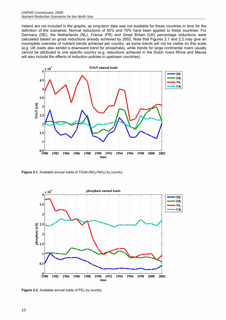
The time series of annual loads for the countries are presented in Figure 2.1 for ToxN and Figure 2.2 for PO4 respectively (NH4 is not presented here). While TOxN (NO3+NO2) displays considerable interannual variability, PO4 has less variability and for most countries a clear reduction signal. The variability in data is caused by interannual variability in river discharges (rainfall), data availability and changes in monitoring practice. TOxN loads are particularly susceptible to variability in rainfall as they are mainly determined by run-off from diffuse sources (agriculture). PO4 loads are to a large extent determined by point sources (waste water and industry), and therefore show less interannual variability. Results for Norway, Ireland and Northern




12

Ireland are not included in the graphs, as long-term data was not available for these countries in time for the definition of the scenarios. Normal reductions of 50% and 70% have been applied to these countries. For Germany (DE), the Netherlands (NL), France (FR) and Great Britain (UK) percentage reductions were calculated based on gross reductions already achieved by 2002. Note that Figures 2.1 and 2.2 may give an incomplete overview of nutrient trends achieved per country, as some trends will not be visible on this scale (e.g. UK loads also exhibit a downward trend for phosphate), while trends for large continental rivers usually cannot be attributed to one specific country (e.g. reductions achieved in the Dutch rivers Rhine and Meuse will also include the effects of reduction policies in upstream countries).

Figure 2.1. Available annual loads of TOxN (NO3+NO2) by country.

Figure 2.2. Available annual loads of PO4 by country.


13

The model setup requires the use of absolute loads in order to complete a realistic hindcast for a particular year. Given the considerable interannual variability and minor apparent changes of TOxN (NO3+NO2), 2002 and 1985 loads were considered as equal (no change). Thus, although Figure 2.1 clearly shows a decreasing trend in TOxN for the Netherlands, the absolute load decrease is taken as 0 as the actual loads for 2002 and 1985 are very similar. The reason for this apparent inconsistency is that 1985 was a dry year with lower than normal run-off. For PO4 and NH4 proportional reductions were calculated as follows:

a. percentage change calculated between 1985 and 2002;

b. rounded to nearest 10% interval to account for variability (uncertainty);

c. only the countries with major rivers for which sufficient data was available were taken into account.

The reductions calculated for 2002 based on the above considerations are presented in Table 2.2. Where a 50% reduction in riverine loads of nitrogen and phosphorus was already met in 2002 compared to 1985, the additional reduction for the scenario was set to zero. Where no long-term data was available (Norway, Ireland, Northern Ireland) a 50% and 70% reduction requirement was applied.

Table 2.2: Shows (a) the reductions in riverine nitrogen and phosphorus loads achieved by Contracting Parties by reducing riverine nutrient inputs for target areas in their waters in the period 1985 – 2002. Next taking into account the reductions already achieved the additional % reduction to be applied for the year 2002 to achieve a 50% (scenario 1: section b) and 70% (scenario 2: section c) reduction scenario for nitrogen and phosphorus in relation to 1985 are shown. The table makes clear that where a Contracting Party has already achieved a 50% or 70% reduction in riverine nutrient loading compared to 1985 (e.g. Germany and the Netherlands for ammonia for the 50% and 70% reduction), then no further reduction is applied in relation to 2002 in order to carry out the specific scenario testing.

Contracting Party TOxN (%) NH4 (%) PO4 (%)

(a) Reductions achieved between 1985 and 2002 Netherlands 0 70 70 Germany 0 90 50 UK 0 20 0 France 0 10 60 (b) Scenario 1: Reductions of 2002 national loads necessary to achieve 50% reduction compared to 1985 Netherlands 50 0 0 Germany 50 0 0 UK 50 40 50 France 50 40 0 (c) Scenario 2: Reductions of 2002 national loads necessary to achieve 70% reduction compared to 1985 Netherlands 70 0 0 Germany 70 0 40 UK 70 60 70 France 70 70 20

Due to lack of data, no load reduction was prescribed for the organic part of the load. A point discussed at the workshop was how the organic load should be reduced in relation to the lowering of the prescribed inorganic loads. First it was considered that organic load consists of i) the organic matter which is degradable within a reasonable time-scale and ii) a refractory part, but that only the degradable part is relevant. The common feeling at the workshop was that the riverine organic load is negligible and that potential shortfalls in riverine organically derived nutrients might be much smaller than internally generated detrital nutrients calculated within the models. Only in local situations, such as shallow areas, e.g. the Wadden Sea or Lake IJssel, may the organic load from terrestrial sources become an important factor. The Oyster Grounds, which are included in the offshore target area (NL-O2) are a temporary sedimentation area, but there the main source of organic load is marine formed within the model domain. Transport processes are the focus of further intersessional OSPAR work on transboundary nutrient transport. The argument was brought forward that measurements tend to underestimate the particulate load of rivers since they are flow dependent and that the organic load is mainly found in the bedload. The general view at the workshop was that estuary models were needed to better understand these processes. However, studies of the Humber estuary as part of a UK project (LOIS) showed that, even when using a multi-model approach which included a catchment, estuarine and coastal model, it was not possible to reconstruct the organic load. Taking into account the differences between estuaries, which are too variable to allow for a generalized conclusion, one approach would be to carry out sensitivity analysis to identify the importance of the organic load and determine the required complexity of the ecosystem model (e.g. the incorporation of zooplankton or bacteria) necessary to


14

address this issue. However, the general conclusion was that organic degradable load seems to be negligible and does not bias the model results.

2.2 Spin-up time The participants had been asked to run their models repeatedly for one year for a sufficient number of years (with a minimum of 3 years) to achieve a repeating seasonal cycle. The year 2002 using 2002 nutrient inputs and boundary conditions was suggested to be repeated 3 times in order to reach a repeating annual cycle indicating that the model is in equilibrium. The end state of this spin-up should be used as a starting condition for the reference (or standard) year 2002 and all reduction scenarios.

It has been noted that more complex models, e.g. with detailed benthic modules, as well as model applications in deeper waters needed more spin-up time than the proposed 3 years. In order to demonstrate that a “stable equilibrium” had been reached the results for a number of relevant variables should show that each of the simulated time series converged.

For the purpose of validating the standard run it would be desirable in future to do the spin up for the years previous to the standard run for 2002, otherwise the comparison with January/February observations are biased. Forcing data are currently available for 2001 and 2002 while future spin-ups with a series of years will be restricted to availability of data and resources for aggregation of common forcing data for application.

Finally, the workshop was convinced that the spin-ups applied for the individual models were carried out successfully to reach a “stable equilibrium”, either by applying longer spin-up times for more complex models or, in shallower coastal areas, by using the proposed 3 years. The spin-up procedure using the year 2002 was accepted to be suitable for reaching a balance between river loads and the system and provided a reliable basis for the simulation. Prolonging the spin-up for a series of years would achieve a further robustness to enhance the model capability to reproduce interannual variability; however, differences in the model results to the proposed adjustments of the spin-up procedure would only be in minor details.

2.3 Boundary conditions In order to achieve a consistent set of boundary data for all model applications as recommended by the last workshop, the only feasible approach was to extract these data from a wider area model whose domain covered the spatial extent of all the other models. Therefore, the boundary data were provided by the Atlantic Margin Model POLCOMS-ERSEM through model runs for 51 pelagic variables for each boundary location of the different national models (Belgium, France, Germany, the Netherlands, Norway, Portugal and the UK (Cefas and POL)). In addition, 12 benthic parameters for the initialisation fields were made available. This consistent dataset was not only provided for the standard run but also for both reduction runs on a daily basis for the year 2002.

2.4 Meteorological forcing With the kind permission of the European Centre for Medium-Range Weather Forecasts (ECMWF), their Operational Data for the years 2001 and 2002 was supplied to workshop participants for use as meteorological forcing data in their simulations. Using the same data ensured consistency with the model used to generate boundary conditions.

2.5 Atmospheric N-deposition The data fields for the atmospheric nitrogen deposition were provided by the Cooperative Programme for Monitoring and Evaluation of the Long-range Transmission of Air Pollutants in Europe (EMEP) on a monthly basis for the years 2001 and 2002. The variables provided included: dry deposition of oxidized nitrogen (NOx); wet deposition of oxidized nitrogen (NOx); dry deposition of reduced nitrogen (NH4); and wet deposition of reduced nitrogen (NH4). Atmospheric deposition of nutrients was not reduced in the reduction scenarios. Following the EUC recommendations, only riverine sources and discharges were reduced in the nutrient reduction scenarios.

An inconsistency in the description of the units of the atmospheric deposition data caused some participants (including POL) to underestimate this forcing by a factor of 12 in the model. This could not be corrected before the workshop. Moreover, some models did not have the capability to include atmospheric deposition. After the workshop POL demonstrated in an additional sensitivity run with the corrected atmospheric deposition that coastal areas are relatively less affected than offshore areas by atmospheric nutrient inputs because of the dominance of riverine nutrient sources. The influence of the underestimate in the POL model run to provide the boundary conditions for the other models is expected to be minor, as the absolute atmospheric deposition decreases with distance from land. Models with a larger domain are expected to be the least affected.


15

2.6 Suspended particulate matter (SPM) Difficulties were reported by workshop participants in forcing the models with SPM data in order to achieve realistic levels of light attenuation, especially for the coastal region. Since in situ observations were regarded as not fit for purpose, different methods were used for SPM forcing of the national model applications. It was noted that, while satellite imagery carried uncertainties, for example due to cloud conditions, modelled SPM concentrations were also subject to uncertainties. Further effort is required to resolve this issue e.g. by combining the best features of satellite imagery (i.e. the gradients and spatial extent) with in situ observations or by using simple SPM model routines that could be shared by all workshop participants.

2.7 Target areas One important change in procedure since the 2005 workshop is the choice of a new set of target areas (see Figure 4.1). These areas correspond roughly to the target areas used in the previous workshop in terms of their location and in their classification as coastal and offshore boxes. However, their shapes have been modified significantly in anticipation of the future work on transboundary nutrient transport. Most of the target areas correspond to areas classified as a ‘problem area’ in German and Dutch maritime waters following the first application of the OSPAR Common Procedure (cf. OSPAR, 2003b). One UK ‘non-problem area’ has been added. The workshop also agreed arrangements for preparing reduction scenarios for two additional target areas covering the Belgian continental shelf and the French coastal waters and for updating this draft assessment with the additional model results in spring 2008.

2.8 Validation data For validation, the year 2002 was chosen as it is the year in which the first application of the OSPAR Common Procedure was carried out and it is also the standard year for the present model applications. A data set to validate the models was provided. In contrast to the 2005 OSPAR workshop, the raw data were made available in a common format, including those outside the target areas. Also, processed maps and cross-sections of temperature and salinity were made available for graphical comparison of the hydrodynamics. For the six target areas an excel spreadsheet was set up to enable the participants to calculate cost functions that had to be used for the validation. This approach aimed at a more rigorous comparison of model performance in order to gauge the uncertainty in model results.

3. Model performance Details of all the models used at the workshop are given in tabular format in Appendix 1. An overview of predictive models for use in eutrophication assessments was recently published by OSPAR (OSPAR, 2008b). The technical details presented provide further information necessary to appreciate the model results. It is clear that the models vary considerably in terms of the formulation of the coupled hydrodynamic and ecological models, since they were designed for answering different questions. A recent review of 3-dimensional coupled hydrodynamic-ecological models, which features some of the models used in this exercise, is provided by Radach and Moll (2006).

3.1 Calibration and validation The calibration procedures adopted by the workshop participants and the details of validation are described in the national presentations. These are hyperlinked and accessible through the workshop report on the Cefas website (www.cefas.co.uk/eutmod).

Data from many sources have been used for validation. Details of the collected and used data are given in the Data Description (ICG-EMO, 2007b). In Figure 3.1 the spatial distribution of all sample locations are given. For each target area (cf. Figure 4.1) and each variable, data from 0 - 15 m depth are combined in surface data, while the deeper samples are combined in bottom samples. Monthly means have been calculated per variable and per target area.





16

Figure 3.1 Spatial distribution of sampling locations from which 2002 data for validation were generated.

As can be seen from Table 3.1 the standard deviations for some of the assessment variables are very large, especially in two of the coastal boxes. A possible explanation can be the heterogeneity of these areas in terms of salinities and subsequently nutrient concentrations. In Table 3.1 also the ranges of the monthly salinities are given. For the areas NL-C3 and G-C1 the ranges are well below salinity 30, indicating the presence of low-salinity samples which can also be traced back to the sampling stations in Figure 3.1.

Table 3.1: Observation data for validation of model results in the target areas (cf. Figure 4.1) giving the mean value (mean), the standard deviation (std) and the number of observations (n) for 2002. The salinity data for the areas NL-C3 and G-C1 were very low, which explains (partly) the high nutrient values.

Winter DIN (µmol/l) Winter DIP (µmol/l) Summer chlorophyll a (µg/l) Salinity in January and February Target

Areas, Fig. 4.1 mean std n mean std n mean std n

O2 mini-mum (mg/l) mean std n Range

UKC1 40.6 21.4 85 1.9 1.2 124 7.7 3.4 271 5.3 33.5 0.8 318 33.0 – 33.8 NLC2 51.6 11.7 8 1.0 0.1 8 11.0 10.1 65 6.9 31.2 3.4 34 30.7 – 31.9 NLC3 84.9 56.5 28 1.3 0.8 28 5.0 3.8 47 6.7 24.2 6.6 27 23.6 – 24.7 NLO2 3.1 0.8 3 0.5 0.05 3 0.6 0.7 144 7.5 32.1 1.2 32 32.1 – 32.1 GC1 127.0 124.7 29 1.4 0.7 29 1.9 1.1 6 4.6 27.6 6.9 20 23.7 – 28.9 GO2 8.2 3.6 6 0.6 0.07 6 0.6 0.4 40 5.5 34.4 0.4 11 34.3 – 34.4 FC2 - - - - - - - - - - - - - FO1 - - - - - - - - - - - - - BC1 25.1 12.6 12 0.8 0.2 12 5.8 4.1 8 9.6 32.1 1.4 25 BO1 17.9 - 1 0.7 - 1 1.6 - 1 9.4 34.1 0.6 5

There were some generic findings from the validation. In general the models perform better in the offshore areas than in the coastal areas. Winter DIN and DIP (defined as mean January and February concentrations) at the surface are in the range of observations or slightly overestimated, while the mean growing season chlorophyll concentrations are overestimated in the offshore areas. All models underestimated winter DIN at the surface and mean growing season chlorophyll concentrations for coastal target areas. Winter DIP is also underestimated in the coastal areas, but to a much lesser extent than winter DIN.


17

Four of the six models (Germany, Netherlands, UK-Cefas and UK-POL) were three-dimensional and provided nutrient concentrations at the surface as well as at the bottom. In most models the differences between surface concentrations and bottom concentrations were zero or negligible. Only the German model gave differences between surface and bottom nutrient concentrations, which were in the range of –7 to +30%. A comparison with measurements has not been made.

One possible explanation for the discrepancy in coastal target areas was cited by a number of workshop participants as due to the heterogeneity of these areas which encompass salinities from 30 – 34.5. The large standard deviations observed in the monitored winter DIN concentrations give credibility to this view (Table 3.1). There was also some misunderstanding by the workshop participants of the guidance provided, such that data associated with salinities outside of the appropriate range for a specific water body type (coastal or offshore) may have been included in post-processing calculations. Dr Lacroix also noted that their Belgian model results were sensitive to the spatial dimensions of the target area. Nevertheless, these validation results were not fully understood and further work is required to establish the reasons for these systematic differences and whether these are specific to each model or result from externally imposed conditions.

3.2 Cost functions To quantify the difference between model results and measurement data we have made use of the cost function as described in Villars & de Vries (1998). The cost function is a mathematical function and gives a non-dimensional number (score), which is indicative of the correspondence between two sets of data. Cost functions as used here should not be interpreted as having any financial element or meaning; their name refers to ‘cost’ merely because of the way they work: a high score is undesirable. The cost function not only compares the model results with the observations, but also accounts for the statistical reliability of the observations. This means that model results that deviate substantially from statistically unreliable measurements may still achieve a score that is as good as, or better than, model results that deviate less from statistically very reliable measurements. In general, the closer the score is to zero, the better the model result. This method makes also comparison between results of different models possible.

For each target area and each variable the participants calculated monthly means of their model results. The monthly means are compared with monthly means of measurements of that variable in the given target area. The outcome of these monthly cost functions can be positive (overestimation) or negative (underestimation). A value zero means that the model results are exactly equal to the measurements. The absolute value depends critically on the standard deviation of the observations. Figure 3.2 shows an example of the performance of three or four models in the Dutch coastal target area NL-C2 for the parameters included in the cost function.


18

NLC2 Temp

-8

-7

-6

-5

-4

-3

-2

-1

0

1

2

3

1 2 3 4 5 6 7 8 9 10 11 12

NL UK-Cef UK-POL

NLC2 Sal

-2

-1.5

-1

-0.5

0

0.5

1

1.5

2

1 2 3 4 5 6 7 8 9 10 11 12

NL UK-Cef UK-POL

NLC2 Din

-8-6-4-202468

101214

1 2 3 4 5 6 7 8 9 10 11 12

NL UK-Cef DE UK-POL

NLC2 DIP

-10

0

10

20

30

40

50

1 2 3 4 5 6 7 8 9 10 11 12

NL UK-Cef DE UK-POL

NLC2 Chla

-6

-4

-2

0

2

4

6

8

10

12

1 2 3 4 5 6 7 8 9 10 11 12

NL UK-Cef DE UK-POL

NLC2 SPM

-2

-1.5

-1

-0.5

0

0.5

1

1 2 3 4 5 6 7 8 9 10 11 12

NL UK-Cef

Figure 3.2. Monthly cost functions for temperature (Temp) (0C), salinity (Sal), DIN, DIP, chlorophyll (Chla), and SPM for four models (Germany, the Netherlands, UK-Cefas and UK-POL) in target area NL-C2. No validation data were available for cost functions for temperature, salinity and SPM from Germany, and for SPM from UK-POL


19

An annual mean value for the cost function has been calculated from the absolute values of the monthly mean cost function. For seven of the variables, in each of the target areas the annual mean cost function is calculated from the results of four models and these are shown in Figure 3.3. To evaluate the performance of a model, Radach and Moll (2006) defined four classes for the values of the cost function: 0-1: excellent; 1-2: good; 2-3: reasonable and values >3: poor.

UKc BE NL DE0

2

4

6

8UKC1

UKc BE NL DE0

2

4

6NLC2

UKc BE NL DE0

5

10

15

20

25NLC3

TemperatureSalinityDINPO4ChlaO2SPMRadach & Moll (2006)

UKc BE NL DE0

5

10

15

20

25NLO2

UKc BE NL DE0

5

10

15

20GC1

UKc BE NL DE0

20

40

60

GO2

Figure 3.3: Annual mean cost functions for the models presented by UK/Cefas (UKc), Belgium (BE), the Netherlands (NL) and Germany (DE) for each target areas. The red horizontal line indicates the boundary between reasonable and poor according to Radach & Moll (2006). Please note that the figure for UK-C1 has an adjusted y-axis: oxygen values for UKc and NL were 78.6 and 130.8 respectively.


20

4. Reduction scenarios For the purposes of the OSPAR Common Procedure, target areas were chosen which encompass offshore areas with salinities > 34.5 and coastal areas with salinities of 30 – 34.5. In general, offshore areas will be deeper and potentially subject to summer time thermal stratification. These offshore waters will also be less turbid with relatively high water clarity. In shallow waters, turbidity is generally higher and light conditions less favourable for growth. In deeper waters ( >60 m approximately), however, waters are optically deep and require the onset of thermal stratification to create a surface mixed layer in which there is sufficient light to enable net phytoplankton growth to occur.

Figure 4.1 Target areas for nutrient reduction scenarios

The results of the nutrient reduction scenarios are presented for those model applications which followed the Workshop User Guide (ICG-EMO, 2007a) and used the same forcing data. The results are presented in the following as real value changes and as % changes of the eutrophication parameters in response to the additional % reductions in nutrient loads calculated for each parameter and target area in relation to 2002 (Table 2.2). Appendix 2 presents the results of the reduction scenarios in the scoring format of the OSPAR Common Procedure. The model results are presented and scored against the area-specific assessment levels for the target area which the relevant Contracting Party used in the first application of the Comprehensive Procedure in 2002 (cf. OSPAR, 2003b). The purpose is to put the model results into the context of the OSPAR Common Procedure and give an indication of direction of change. The assessment levels of 2002 were chosen to ensure comparability of the model results with the monitoring-based Common Procedure results, especially when comparing the scoring results for the year 2002.

For each of the target areas two sets of figures are presented. The first set presents a summary of the % reduction achieved in selected assessment variables for the specific two reduction scenarios for the year 2002 (Table 2.2), and include a mean % reduction derived from all of the model results available for that parameter and target area. The first set of figures (e.g. Figure 4.2), termed ‘response plots’, enables more ready comparison between models in terms of sensitivity and the robustness of conclusions drawn from the nutrient reduction scenarios. Calculation of the % reduction is carried out in the following manner:

For a given model the concentration of the simulated assessment variable in the reduction scenario is converted to a percentage where the standard run (for the year 2002 without reduction in riverine




21

nutrients) is regarded as representing the 100% value. This calculation is carried out for each target area, for each model and the results presented separately for winter DIN, winter DIP, mean chlorophyll and minimum dissolved oxygen concentration.

The second set of figures (e.g. Figure 4.3) presents the results of reduction scenarios in terms of concentrations for each of the assessment parameter for all of the models for each target area. These figures make it possible to better judge the differences between model results based on simulated concentrations.

The new steps introduced into the present procedures for testing nutrient reduction scenarios have increased comparability between model results. In particular, the specification of a minimum spin-up of 3 years (a number of workshop participants used a larger number of years), shared boundary conditions and improvements in forcing data, all contributed to the increase in comparability and in confidence in the individual model application.

Apart from new procedures designed to improve comparability between model results it is worth noting that all workshop participants carried out model calibration and validation procedures based on the supplied original data. Also, salinity and temperature data were made available from the German Federal Agency for Shipping and Hydrography (BSH) for comparison with model results. The extent of the validation carried out by workshop participants varied with some going beyond the minimum requirements described in the User Guide. The introduction and future use of cost functions (Section 3.2) was welcomed at the workshop but it was noted that the mismatch between the large number of data points from the models and generally low number of observations used to calculate the cost function in this exercise reduced its reliability. Therefore, the confidence attributed to the performance of an individual model is based primarily upon the outcome of the validation procedure rather than on the results of the cost function calculation.

A range of models was used in the reduction scenarios. Appendix 1 gives an overview of the models used and their different features. The differences in models result in differences in model responses to nutrient reduction scenarios and this despite the use of the same forcing data. This includes e.g. differences in the sensitivity of the model to a particular parameter. If despite all differences, the results of the models show the same trend this means an increased level of confidence in the model result.

To indicate a level of confidence in the outcome to nutrient reduction scenarios, a tentative assessment of confidence is made based upon the following criteria:

Criterion 1: the level of agreement, in terms of simulated concentrations, between model results for the same assessment parameters;

Criterion 2: the degree of similarity between the gradients of the ‘response plots’.

So, where the range of simulated values (criteria 1) from all available model results, for example of winter DIN for the UK coastal target area, is similar (based on a visual inspection of the data), and where there is an acceptable degree of similarity (established by visual inspection of the data) between the slopes of the response lines (criteria 2), then a high confidence is attributed to that set of results. If only one of the two criteria has been reached, the attributed confidence is medium. If both criteria are not deemed to have been fulfilled, only a low confidence can be attributed. The limitations of this approach to determining the level of confidence in the results of the reduction scenario are recognised, and it may be that further work is carried out to improve the method. It should also be noted that failure to attribute high confidence to the ensemble of model results for certain target areas and/or parameters does not mean that the results are unreliable rather that more caution may be required in drawing conclusions about the specific outcome to a nutrient reduction scenario. A deliberately cautious method has been taken to the assessment of confidence.

The specific % reduction in riverine nutrient loads in relation to 2002 results from a composite reduction made up of the specific reductions, calculated for each country (see scenario 1 and 2 in Table 2.2). This means that the specific reduction scenarios need to be taken into account in the interpretation of the assessment parameter results for each target area. This is particularly obvious for phosphorus for which considerable load reductions had been achieved by Contracting Parties in the past and little if any additional reductions were applied for 2002 to achieve a 50%/70% reduction in relation to 1985; as a consequence, winter DIP concentrations show a limited response in the reduction scenarios. It should be noted that the Norwegian and French results are not included in the calculation of average % changes in the assessment parameters. This is because, due to lack of time, the workshop procedures were not carried out according to the User Guide. However, results are shown in the figures that display changes in assessment parameters in terms of concentration. German results for oxygen have been excluded from the G-O2 target area results.


22

4.1 German offshore target area: G-O2 This is an offshore water body that is situated close to the northern boundary of the models. It is relatively deep and is subject to summer time thermal stratification.

DIN

On average a 24% reduction in winter DIN is achieved with scenario 1 and 31% reduction with scenario 2. There is a wide range of simulated concentrations in the standard run but much less variability in concentrations for the reduction scenarios. Differences in the gradients of the response plots result in designating the results as of low confidence.

DIP

On average a 6% reduction in winter DIP is achieved with scenario 1 and 10% reduction with scenario 2. Model responsiveness is low and similar for the 4 models applied. It should be noted that the DIP reductions in the river loads are small in the German rivers. However, the range of simulated concentrations that vary by a factor of >2 lead to classification as results with a medium confidence level.

Chlorophyll

On average a 9% reduction in chlorophyll is achieved with scenario 1 and 14% reduction with scenario 2. Model sensitivity is low and similar for the four models applied. Agreement between the model results provides high confidence in this result.

Oxygen

On average a 5% increase in minimum dissolved oxygen concentration is achieved with scenario 1 and 7% increase with scenario 2. Model responsiveness is very similar for the three sets of model results considered. The relatively limited range of simulated concentrations leads to a high confidence in this result.

G-O2 - parameter response to scenario 1

0 10 20 30 40 50 60

DIN DIP Chl O2min

redu

ctio

n (%

)

UK-Cef DE NL UK-POL mean

G-O2 - parameter response to scenario 2

0

10

20

30

40

50

60

DIN DIP Chl O2min

redu

ctio

n (%

)

UK-Cef DE NL NO UK-POL mean

Figure 4.2 % reduction in mean winter DIN and DIP and mean summer chlorophyll (Chl), and % increase in annual minimum oxygen (O2min) computed by the different models as a response to the reduction scenarios 1 and 2 (see Table 2.2). Norway did not simulate scenario 2; there are no minimum oxygen data for Germany. The average of the different models (mean % reduction in parameter level) does not include UK-POL results due to uncertainties in the post-processing. This is the case for all such calculations in this section of the report.


23

G-O2 - mean winter DIN at surface

02468

10121416

0 20 40 60 80

nutrient load reduction (%)

µmol

/l

G-O2 - mean winter DIP at surface

0

0.2

0.4

0.6

0.8

1

0 20 40 60 80


µmol

/l

G-O2 - mean summer chlorophyll at surface

0

1

2

3

4

0 20 40 60 80


µg/l

UK-Cef DE NLNO UK-POL ass. level

G-O2 - annual oxygen minimum at bottom

0

2

4

6

8

10

0 20 40 60 80


mg/

l


Figure 4.3 Concentrations of mean winter DIN and DIP at the surface, mean summer chlorophyll at the surface, and annual minimum oxygen concentration at the bottom for the year 2002 (standard run at 0% reduction) and for the reduction scenarios 1 and 2 (see Table 2.2). Norway did not simulate scenario 2 and there are no minimum oxygen data from Germany. The concentrations are shown against the assessment levels (ass. level) used by Germany for their areas reflected in the target box in the first application of the Comprehensive Procedure (OSPAR publication 189/2003).


24

4.2 Netherlands offshore area: NL-O2 This is an offshore (> 34 salinity) water body with summer thermally stratified waters, ranging from approximately 40 – 80 m depth.

DIN

On average a 19% reduction in winter DIN is achieved with scenario 1 and 25% reduction with a scenario 2. Model responsiveness varied and despite different starting concentrations in the standard run for each model the results tended to converge resulting in a similar simulated concentration for each model for each scenario. Although confidence criterion 1 is fulfilled, criterion 2 is only partially fulfilled, and consequently only a medium confidence is attributed to these results.

DIP

On average a 5% reduction in winter DIP is achieved with scenario 1 and 10% reduction with scenario 2. Model responsiveness is similar between three of the four models considered. However, the range of simulated concentrations showed a degree of variability that on balance fails to fulfil confidence criterion 1; therefore a medium confidence in assigned to the results.

Chlorophyll

On average a 5 % reduction in chlorophyll is achieved with scenario 1 and 7% reduction with a scenario 2. Low and similar responsiveness was apparent in all model results accounting for the relatively small changes in simulated chlorophyll concentrations observed. However, the range of simulated concentrations showed a degree of variability that on balance fails to fulfil confidence criterion 1, leading to a classification of the result as having medium confidence.

Oxygen

On average a 6% increase in minimum dissolved oxygen concentration is achieved with scenario 1 and 10% increase with scenario 2. Model responsiveness is very similar for 2 of the 3 model results. The range of simulated concentrations is < 1 mg/l. A precautionary approach does not lead to a conclusion of high confidence in this result.

NL-O2 - parameter response to scenario 1

0

10

20

30

40

50

DIN DIP Chl O2min

redu

ctio

n (%

)


NL-O2 - parameter response to scenario 2

0

10

20

30

40

50

DIN DIP Chl O2min

redu

ctio

n (%

)


Figure 4.4 % reduction in mean winter DIN and DIP and mean summer chlorophyll (Chl), and % increase in annual minimum oxygen (O2min) computed by the different models as a response to the reduction scenarios 1 and 2 (see Table 2.2). There are no minimum oxygen data from Germany.


25

NL-O2 - mean winter DIN at surface

02468

10121416

0 20 40 60 80


µmol

/l

NL-O2 - mean winter DIP at surface

0

0.2

0.4

0.6

0.8

1

0 20 40 60 80


µmol

/l

NL-O2 - mean summer chlorophyll at surface

0

1

2

3

4

5

0 20 40 60 80


µg/l


NL-O2 - annual oxygen minimum at bottom

4

5

6

7

8

9

0 20 40 60 80


mg/

l


Figure 4.5 Concentrations of mean winter DIN and DIP at the surface, mean summer chlorophyll at the surface, and annual minimum oxygen concentration at the bottom for the year 2002 (standard run at 0% reduction) and for the reduction scenarios 1 and 2 (see Table 2.2). Norway did not simulate scenario 2 and there are no minimum oxygen data for Germany. The concentrations are shown against the assessment levels used by the Netherlands for their areas reflected in the target box NL-O2 in the first application of the Comprehensive Procedure (OSPAR publication 189/2003).


26

4.3 Netherlands coastal waters: NL-C2 This is a coastal water body that includes Rhine waters with salinities at a range from 32 – 33 and depths from 5 m close to the coast to 20 m farther from the coast (source: http://www.noordzeeatlas.nl).

DIN

On average a 41% reduction in winter DIN is achieved with scenario 1 and 56% reduction with scenario 2. Model responsiveness was very similar for the four simulations considered. The range of simulated concentrations for the reduction scenarios varies by a factor of about 2 and therefore the results are classified as of medium confidence.

DIP

On average a 6% reduction in winter DIP is achieved with scenario 1 and a 9% reduction with scenario 2. There is a relatively large range in model results for the reduction scenarios. Responsiveness of three of the four models considered is similar. Therefore, it is possible to designate the result as of medium confidence. Chlorophyll

On average a 4% reduction in chlorophyll is achieved with scenario 1 and 9% reduction with scenario 2. Low responsiveness was apparent in all model results accounting for the relatively small changes observed. One model showed a slightly higher degree of responsiveness. There is a relatively large range in model results between the reduction scenarios. Therefore, the results are classified as of medium confidence. Oxygen

On average a 0% increase in minimum dissolved oxygen concentration is achieved with scenario 1 and a 1% increase with scenario 2. Model responsiveness is very similar for the two model results. The range of simulated oxygen concentrations is relatively narrow. The agreement between the model results provides medium confidence in this result.

NL-C2 - parameter response to scenario 1

0 10 20 30 40 50 60 70

DIN DIP Chl O2min

redu

ctio

n (%

)



0

10

20

30

40

50

60

70

DIN DIP Chl O2min

redu

ctio

n (%

)




27

NL-C2 - mean winter DIN at surface

0102030405060

0 20 40 60 80


µmol

/l

NL-C2 - mean winter DIP at surface

0

0.4

0.8

1.2

1.6

0 20 40 60 80


µmol

/l

NL-C2 - mean summer chlorophyll at surface

02468

10121416

0 20 40 60 80


µg/l


NL-C2 - annual oxygen minimum at bottom

4

5

6

7

8

0 20 40 60 80


mg/

l


Figure 4.7 Concentrations of mean winter DIN and DIP at the surface, mean summer chlorophyll at the surface, and annual minimum oxygen concentration at the bottom for the year 2002 (standard run at 0% reduction) and for the reduction scenarios 1 and 2 (see Table 2.2). Norway did not simulate a scenario 2 and there are no minimum oxygen data from Germany. The concentrations are shown against the assessment levels (ass. level) used by the Netherlands for their areas reflected in the target box NL-C2 in the first application of the Comprehensive Procedure (OSPAR publication 189/2003).


28

4.4 Netherlands coastal waters: NL-C3 This is a coastal water body outside the barrier islands without Wadden Sea and Ems estuary. Salinities are in the range of 30 – 34.5 and depths are from 5 m close to the coast to 30 m farther from the coast (source: www.noordzeeatlas.nl).

DIN

On average a 39% reduction in winter DIN is achieved with scenario 1 and 53% reduction with scenario 2. Model responsiveness was very similar for the four simulations and there was good agreement between simulated concentrations for the two scenarios. In conclusion there is high confidence in the model results.

DIP

On average a 7% reduction in winter DIP is achieved with scenario 1 and 9% reduction with scenario 2. Model responsiveness is similar between the four models with three of the four models in close agreement in scenario 1. There is medium confidence in the result as after an initial small reduction in DIP no further reduction in DIP is achieved in scenario 2.

Chlorophyll

On average a 6% reduction in chlorophyll is achieved with scenario 1 and 12% reduction with scenario 2. A similar responsiveness was apparent in all model results accounting for the relatively small changes observed. Agreement between the four models results provides high confidence in this result.

Oxygen

On average a 1% increase in minimum dissolved oxygen concentration is achieved with scenario 1 and 2% increase with scenario 2. Model sensitivity is low and very similar for the three model results. The range of model results varies by < 1 mg/l and is regarded as fulfilling the requirements of confidence criterion 1. Therefore, the results are regarded as having high confidence.


0 10 20 30 40 50 60 70

DIN DIP Chl O2min

redu

ctio

n (%

)



0

1020

30

40

50

60

70

DIN DIP Chl O2min

redu

ctio

n (%

)




29

NL-C3 - mean winter DIN at surface

0

10

20

30

40

50

0 20 40 60 80


µmol

/l

NL-C3 - mean winter DIP at surface

0

0.4

0.8

1.2

0 20 40 60 80


µmol

/l

NL-C3 - mean summer chlorophyll at surface

02468

10121416

0 20 40 60 80


µg/l


NL-C3 - annual oxygen minimum at bottom

4

5

6

7

8

0 20 40 60 80


mg/

l


Figure 4.9 Concentrations of mean winter DIN and DIP at the surface, mean summer chlorophyll at the surface, and annual minimum oxygen concentration at the bottom for the year 2002 (standard run at 0% reduction) and for the reduction scenarios 1 and 2 (see Table 2.2). Norway did not simulate scenario 2 and there are no minimum oxygen data from Germany. The concentrations are shown against the assessment levels (ass. level) used by the Netherlands for their areas reflected in the target box NL-C3 in the first application of the Comprehensive Procedure (OSPAR publication 189/2003).


30

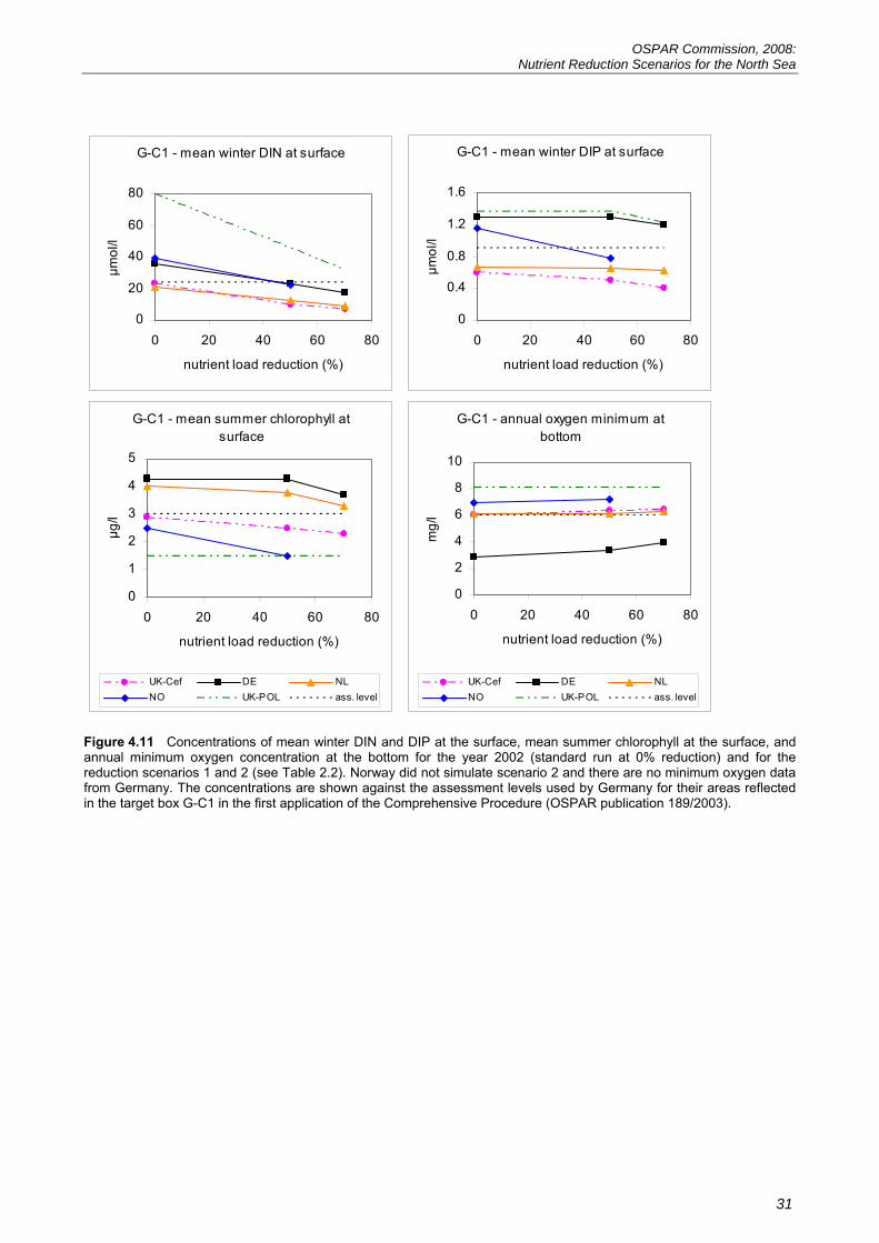
4.5 German coastal waters: G-C1 The target area G-C1 is located within the German Bight, a shallow bight with a water depth mostly below 40 m. This coastal water body with salinities between 30 and 34.5 receives large amounts of nutrients from the rivers Elbe, Weser and Ems, and from transboundary transport along with the coastal currents.

DIN

On average a 44% reduction in winter DIN is achieved with scenario 1 and 60% reduction with scenario 2. Model responsiveness was quite pronounced and very similar for the four simulations. The good agreement between the four models in terms of the range of values for the simulations together with similar model responsiveness provides high confidence in this result.

DIP

On average a 5% reduction in winter DIP is achieved with scenario 1 and 15% reduction with scenario 2. Model responsiveness tends to vary down to the 50% reduction and thereafter is similar. The simulated DIP concentrations are relatively widespread. Consequently, these results are regarded as having low confidence.

Chlorophyll

On average a 5% reduction in chlorophyll is achieved with scenario 1 and 13% reduction with scenario 2. Low and, to some extent, variable responsiveness was apparent in model results accounting for the relatively small changes observed. The range of simulated chlorophyll concentrations varies by a factor of approximately 3. Consequently, these results are regarded as having low confidence.

Oxygen

On average a 6% increase in minimum dissolved oxygen concentration is achieved with scenario 1 and 12% increase with scenario 2. Model responsiveness is very similar for the three model results and the range of results varies by < 1 mg/l. Consequently, these results are regarded as having high confidence.

G-C1 - parameter response to scenario 1

0 10 20 30 40 50 60 70 80

DIN DIP Chl O2min

redu

ctio

n (%

)


G-C1 - parameter response to scenario 2

01020304050607080

DIN DIP Chl O2min

redu

ctio

n (%

)




31

G-C1 - mean winter DIN at surface

0

20

40

60

80

0 20 40 60 80


µmol

/l

G-C1 - mean winter DIP at surface

0

0.4

0.8

1.2

1.6

0 20 40 60 80


µmol

/l

G-C1 - mean summer chlorophyll at surface

0

1

2

3

4

5

0 20 40 60 80


µg/l


G-C1 - annual oxygen minimum at bottom

0

2

4

6

8

10

0 20 40 60 80


mg/

l


Figure 4.11 Concentrations of mean winter DIN and DIP at the surface, mean summer chlorophyll at the surface, and annual minimum oxygen concentration at the bottom for the year 2002 (standard run at 0% reduction) and for the reduction scenarios 1 and 2 (see Table 2.2). Norway did not simulate scenario 2 and there are no minimum oxygen data from Germany. The concentrations are shown against the assessment levels used by Germany for their areas reflected in the target box G-C1 in the first application of the Comprehensive Procedure (OSPAR publication 189/2003).


32

4.6 UK coastal waters: UK-C1 This is a coastal water body with salinities of 30 – 34.5. It is well mixed with respect to density and relatively turbid. DIN On average a 30% reduction in winter DIN is achieved with scenario 1 and 41% reduction with scenario 2. There are differences in model responsiveness with the range of simulated DIN concentrations varying by a factor of approximately 2. Consequently, these results are regarded as having medium confidence. DIP On average a 22% reduction in winter DIP is achieved with scenario 1 and 30% reduction with scenario 2. There is considerable variability in the starting concentrations and, although there is some convergence in model results in scenario 2, large differences remain. The variability in model results leads to a medium confidence in the result. Chlorophyll On average a 18% reduction in chlorophyll is achieved with scenario 1 and 25% reduction with scenario 2. Model responsiveness varies between models and the range of simulated DIP concentrations is quite wide. In conclusion, the results are regarded as having low confidence. Oxygen On average a 2% increase in minimum dissolved oxygen concentration is achieved with scenario 1 and 3% increase with scenario 2. Model responsiveness is very similar for the 4 model results. The range of simulated dissolved oxygen is < 1 mg/l and thus the results are regarded as having high confidence.

UK-C1 - parameter response to scenario 1

0 10 20 30 40 50 60 70

DIN DIP Chl O2min

redu

ctio

n (%

)

BE UK-Cef DE NL UK-POL mean

UK-C1 - parameter response to scenario 2

0

10

20

30

40

50

60

70

DIN DIP Chl O2min

redu

ctio

n (%

)

BE UK-Cef DE NL UK-POL mean

Figure 4.12 % reduction in mean winter DIN and DIP and mean summer chlorophyll (Chl), and % increase in annual minimum oxygen (O2min) computed by the different models as a response to the reduction scenarios 1 and 2 (see Table 2.2). There are no minimum oxygen data from Belgium.


33

UK-C1 - mean winter DIN at surface

05

1015202530

0 20 40 60 80


µmol

/l

UK-C1 - mean winter DIP at surface

0

0.4

0.8

1.2

1.6

2

0 20 40 60 80


µmol

/l

UK-C1 - mean summer chlorophyll at surface

0 2 4 6 8

10 12 14 16

0 20 40 60 80


µg/l

BE UK-Cef DE NL NO UK-POLFR ass. level

UK-C1 - annual oxygen minimum at

bottom

4

5

6

7

8

0 20 40 60 80 nutrient load reduction (%)

mg/

l

BE UK-Cef DE NL NO UK-POL FR ass. level

Figure 4.13 Concentrations of mean winter DIN and DIP at the surface, mean summer chlorophyll at the surface, and annual minimum oxygen concentration at the bottom for the year 2002 (standard run at 0% reduction) and for the reduction scenarios 1 and 2 (see Table 2.2). Norway did not simulate scenario 2 and there are no minimum oxygen data from Belgium. The concentrations are shown against the assessment levels (ass. level) used by the UK for their areas reflected in the target box UK-C1 in the first application of the Comprehensive Procedure (OSPAR publication 189/2003).


34

4.7 Belgian coastal waters: BE-C1 This is a coastal water body with salinities of 30 – 34.5. It is well mixed with respect to density and relatively turbid compared to offshore waters. DIN On average a 27% reduction in winter DIN is achieved with scenario 1 and 36% reduction with scenario 2. There is a wide range in concentration values, even in the reduction runs, and two distinct sets of gradients. This leads to a classification of the results as low confidence. DIP On average a 1% reduction in winter DIP is achieved with scenario 1 and 1% reduction with scenario 2. Model responsiveness for this assessment parameter is low in this target area, resulting in a reasonable range of values with almost no gradient. This may be due to the already achieved reductions in phosphate inputs, with apparently limited influence of UK rivers in this area. Note the response of the French model, which actually predicts an increase in winter DIP as a result of the reduction scenarios: this may be due to reduced uptake of phosphate as organisms become increasingly nitrogen limited. Overall, given the range of values predicted, these results are classified as medium confidence. Chlorophyll On average a 10% reduction in chlorophyll is achieved with scenario 1 and 18% reduction with scenario 2. Here, the models show good agreement on both values and gradient, giving the results a high confidence level. Oxygen On average a 1% increase in minimum dissolved oxygen concentration is achieved with scenario 1 and 2. The models predict a limited range of values, with small but different gradients. Due to the number of models used here and the range in values this result is classified at the medium confidence level.

BE-C1 - parameter response scenario 1

0 10 20 30 40 50 60

DIN DIP Chl O2min

redu

ctio

n (%

)

BE UK-Cef DE NL mean

BE-C1 - parameter response to scenario 2

0

10

20

30

40

50

60

DIN DIP Chl O2min

redu

ctio

n (%

)


Figure 4.14 % reduction in mean winter DIN and DIP and mean summer chlorophyll (Chl), and % increase in annual minimum oxygen (O2min) computed by the different models as a response to the reduction scenarios 1 and 2 (see Table 2.2). There are no minimum oxygen data from Germany and Belgium.


35

BE-C1 - mean winter DIN at surface

05

1015202530

0 20 40 60 80


µmol

/l

BE-C1 - mean winter DIN at surface

05

1015202530

0 20 40 60 80


µmol

/l

BE-C1 - mean summer chlorophyll at surface

0 2 4 6 8

10 12 14 16

0 20 40 60 80


µg/l

BE UK-Cef DENL FR ass. level

BE-C1 - annual oxygen minimum at bottom

4

5

6

7

8

0 20 40 60 80


mg/

l

BE UK-Cef DE NL FR ass. level

Figure 4.15 Concentrations of mean winter DIN and DIP at the surface, mean summer chlorophyll at the surface, and annual minimum oxygen concentration at the bottom for the year 2002 (standard run at 0% reduction) and for the reduction scenarios 1 and 2 (see Table 2.2). There are no minimum oxygen data from Germany and Belgium. The concentrations are shown against the assessment levels used by Belgium for their areas reflected in the target box BE-C1 in the first application of the Comprehensive Procedure (OSPAR publication 189/2003).


36

4.8 Belgian offshore waters: BE-O1 This is an offshore water body with salinities of > 34.5. It is well mixed with respect to density and relatively turbid compared to deeper northerly waters.

DIN

On average a 17% reduction in winter DIN is achieved with scenario 1 and 24% reduction with scenario 2. The models predict a wide range of values (variation by a factor > 2) and different slopes. As a consequence this result is designated as having low confidence.

DIP

On average a 1% reduction in winter DIP is achieved with scenario 1 and 5% reduction with scenario 2. The large response observed in scenario 2 is mainly due to the German results. Nevertheless, a wide range of values is predicted with different gradients, leading to a classification of low confidence. Chlorophyll

On average a 7% reduction in chlorophyll is achieved with scenario 1 and 9% reduction with scenario 2. Model responsiveness is very similar for all applied models, with similar values and gradients. This leads to a classification of the results as high confidence.

Oxygen

On average a 0% increase in minimum dissolved oxygen concentration is achieved with scenario 1 and 1% with scenario 2. Again, a limited range of values is predicted for minimum bottom oxygen, with little response to the reduction scenarios, resulting in a classification of medium confidence due to the different observed gradients.

BE-O1 - parameter response scenario 1

0 5

10 15 20 25 30 35 40

DIN DIP Chl O2min

redu

ctio

n (%

)


BE-O1 - parameter response to scenario 2

05

10152025

30

3540

DIN DIP Chl O2min

redu

ctio

n (%

)




37

BE-O1 - mean winter DIN at surface

0

5

10

15

20

0 20 40 60 80


µmol

/l

BE-O1 - mean winter DIP at surface

0

0.2

0.4

0.6

0.8

1

0 20 40 60 80


µmol

/l

BE-O1 - mean summer chlorophyll at surface

0 2 4 6 8

10 12 14 16

0 20 40 60 80


µg/l

BE UK-Cef DE NL ass. level

BE-O1 - annual oxygen minimum at

bottom

4

5

6

7

8

9


mg/

l


Figure 4.17 Concentrations of mean winter DIN and DIP at the surface, mean summer chlorophyll at the surface, and annual minimum oxygen concentration at the bottom for the year 2002 (standard run at 0% reduction) and for the reduction scenarios 1 and 2 (see Table 2.2). There are no minimum oxygen data from Germany and Belgium. The concentrations are shown against the assessment levels used by Belgium for their areas reflected in the target box BE-O1 in the first application of the Comprehensive Procedure (OSPAR publication 189/2003).


38

4.9 French coastal waters: F-C2 This is a coastal water body with salinities of 30 – 34.5. DIN On average a 29% reduction in winter DIN is achieved with scenario 1 and 39% reduction with scenario 2. There is a wide range of initial values but with mostly similar slopes. This leads to a classification of medium confidence. DIP On average a 1% reduction in winter DIP is achieved with scenario 1 and 2% reduction with scenario 2. A wide range of starting concentrations but similar responsiveness confers a classification of medium confidence. Chlorophyll On average a 9% reduction in chlorophyll is achieved with scenario 1 and 16% reduction with scenario 2. Agreement between initial concentrations is reasonable with a similar responsiveness between models is found. This leads to a classification of medium confidence. Oxygen

On average a 1% increase in minimum dissolved oxygen concentration is achieved with scenario 1 and with scenario 2. There is a reasonable level of agreement between initial concentrations and responsiveness is very similar giving medium confidence to these results.

F-C2 - parameter response to scenario 1

0

10

20

30

40

50

DIN DIP Chl O2min

redu

ctio

n (%

)


F-C2 - parameter response to scenario 2

0

10

20

30

40

50

DIN DIP Chl O2min

redu

ctio

n (%

)




39

F-C2 - mean winter DIN at surface

05

1015

2025

30

0 20 40 60 80


µmol

/l

F-C2 - mean winter DIP at surface

00.20.40.60.8

11.21.4

0 20 40 60 80


µmol

/l

F-C2 - mean summer chlorophyll at surface

0 1 2 3 4 5

0 20 40 60 80


µg/l


F-C2 - annual oxygen minimum at

bottom

4

5

6

7

8


mg/

l


Figure 4.19 Concentrations of mean winter DIN and DIP at the surface, mean summer chlorophyll at the surface, and annual minimum oxygen concentration at the bottom for the year 2002 (standard run at 0% reduction) and for the reduction scenarios 1 and 2 (see Table 2.2). There are no minimum oxygen data from Germany and Belgium. The concentrations are shown against the assessment levels used by France for their areas reflected in the target box F-C2 in the first application of the Comprehensive Procedure (OSPAR publication 189/2003).


40

4.10 French offshore waters: F-O1 This is an offshore water body with salinities of > 34.5. DIN On average a 10% reduction in winter DIN is achieved with scenario 1 and 14% reduction with scenario 2. Three out of four models are in close agreement for the standard run (0% reduction) and the responsiveness is very similar for all results. This leads to a classification of medium confidence. DIP On average a there is a < 1% reduction in winter DIP with scenario 1 and with scenario 2. There is medium confidence in these results with a range of approximately 0.4 μM PO4 but with similar responsiveness. Chlorophyll On average a 4% reduction in chlorophyll is achieved with scenario 1 and 7% reduction with scenario 2. Similar starting concentrations and responsiveness lead to a classification of high confidence. Oxygen On average a 2% increase in minimum dissolved oxygen concentration is achieved with scenario 1 and with scenario 2. Three model results show similar responsiveness but a wide range of starting concentrations. This leads to a classification of medium confidence.

F-O1 - parameter response to scenario 1

0

5

10

15

20

25

DIN DIP Chl O2min

redu

ctio

n (%

)


F-O1 - parameter response to scenario 2

0

5

10

15

20

25

DIN DIP Chl O2min

redu

ctio

n (%

)




41

F-O1 - mean winter DIN at surface

02468

10121416

0 20 40 60 80


µmol

/l

F-O1 - mean winter DIP at surface

00.20.40.60.8

11.21.4

0 20 40 60 80


µmol

/l

F-O1 - mean summer chlorophyll at surface

0 1 2 3 4 5

0 20 40 60 80


µg/l


F-O1 - annual oxygen minimum at

bottom

2345678


mg/

l


Figure 4.21 Concentrations of mean winter DIN and DIP at the surface, mean summer chlorophyll at the surface, and annual minimum oxygen concentration at the bottom for the year 2002 (standard run at 0% reduction) and for the reduction scenarios 1 and 2 (see Table 2.2). There are no minimum oxygen data from Germany and Belgium. The concentrations are shown against the assessment levels used by France for their areas reflected in the target box F-O1 in the first application of the Comprehensive Procedure (OSPAR publication 189/2003).


42

4.11 Summary The results of the simulation of nutrient reduction scenarios in terms of % reductions in assessment parameters (% increase for oxygen) are summarised and presented in Table 4.1.1 In general, largest reductions in category I parameters (nutrient enrichment) are seen in the coastal water target areas. The model results imply a strong, almost linear response in winter DIN concentrations to the reduced loads. Offshore the decreases are still pronounced in DIN but less so in DIP. Winter DIP concentrations do not respond as strongly to the load reductions as DIN with a decrease of up to 30% in scenario 2 in UK coastal waters but results are typically < 30% for all other areas and scenarios. As already noted earlier the results for winter DIP reflect the fact that for continental rivers an approximately 50% reduction in riverine inputs had already been achieved for Germany, Netherlands and France (see Table 2.2).

The overall range of responses in the category II (direct effects) parameter mean summer chlorophyll concentration is 4% - 25% with similar minimum decreases in coastal and offshore waters but the maximum decreases in coastal waters are nearly double those achieved in offshore areas for both scenarios.

The category III (indirect effects) parameter minimum dissolved oxygen concentration increased by a maximum of 12% for scenario 2 in coastal waters. Offshore and coastal waters gave similar results for both scenarios.

Table 4.1 A summary of the results showing the range of % average decreases in concentration of the winter DIN, winter DIP and mean growing season chlorophyll concentration and % increase for minimum oxygen concentration following scenario 1 and 2 (50% and 70 % reduction in riverine nutrient loads in respect to 1985) for four coastal and two offshore target areas. Results from Norway and France are not included here, as they did not follow the prescribed procedure.

Assessment parameters Category I

(nutrient enrichment) Category II

(direct effects) Category III

(indirect effects) Water type

Reduction scenario

DIN DIP Mean Chl O2 min max min max min max min max

Sc1 27 44 1 22 4 18 0 6 Coastal Sc2 36 59 1 30 9 25 1 12 Sc1 10 24 0 6 4 9 0 6 Offshore Sc2 14 31 0 10 7 14 1 10

5. Discussion The workshop agreed that the new procedures introduced since the 2005 OSPAR workshop in Hamburg had achieved the aim of reducing uncertainty in the model results from the nutrient reduction scenario experiments. Notably the provision of common boundary conditions, increased spin-up time, further improvements in the shared riverine nutrient input data, common meteorological data and atmospheric data considerably improved comparability between model results. As a result of these and other improved procedures adopted for this latest workshop confidence in the outcome has improved.

By considering the reductions in riverine nutrient inputs for nitrogen and phosphorous already achieved by Contracting Parties since 1985 (Table 2.2), more realistic reduction scenarios have been constructed. The riverine inputs for individual rivers themselves have been improved. For example, an improved interpolation technique was adopted for the UK rivers to deal with any gaps in observations. Even though the river data provided for the workshop had achieved the best coverage in space and time that was available in the modelling community to date there are some limitations in these data arising from poor temporal resolution of the measured nutrient concentrations. In addition, and more recently, there has been a tendency to stop measurement of silicate concentration in continental rivers.

To aid assessment of individual model performance, the use of cost functions has been introduced. This is regarded as a useful mechanism for judging performance and further contributing to confidence in the outcome of the workshop. The method of application should be refined, however, as the use of temporal and spatial averages was found to bias the results towards poor scores when observational data were sparse or

1 The OSPAR Common Procedure provides a set of harmonised assessment parameters which are classified in four categories expressing causative factors, i.e. nutrient enrichment (category I), direct effects of nutrient enrichment (category II), indirect effects of nutrient enrichment category III) and other possible effects of nutrient enrichment (category IV) (OSPAR 2005).


43

irregular in time and/or space. Also, concern was expressed about the choice of the cost function used. Hence, the present cost function scores should be interpreted with extreme caution.

Whilst many improvements had been made to the procedures, the workshop concluded that future work would benefit from a shared solution to generating fields for suspended particulate matter (SPM) either through making use of remote and in situ measurements or by the use of simple SPM model routines that could be shared by participants. SPM is important as it is the most important explanatory variable for light attenuation in the models. Nevertheless, most participants had made advances since the previous workshop.

The reduction scenarios demonstrated clear differences between coastal and offshore target areas in terms of the response of assessment parameters to reduction in nutrient loads. For winter DIN highest percentage reductions took place in coastal waters while for winter DIP much smaller reductions were evident for coastal and offshore areas. The highest reductions in winter DIP occurred in the UK and German coastal target areas and the least reductions in Dutch waters. The result reflects the fact that the Netherlands and Germany had already achieved significant reductions in their riverine loads of phosphorus as noted earlier (see section 2.1). Reduction scenario 1 for the Netherlands and Germany required no change in the actual river load for phosphorus since the reduction, in comparison to 1985, had already reached this level. For the Netherlands this was also the case for reduction scenario 2, while for Germany a reduction of 40 % (of 2002 values) in phosphorus load was still required.

For mean summer chlorophyll concentrations greatest reductions took place in coastal target areas with a much greater reduction in the UK target area. However, apart from that target area, this parameter was not highly responsive to reduced nutrient loading. This does not imply that there is no response in the modelled biological system, but only that this assessment parameter is relatively insensitive to the level of the nutrient load. It was recognised by the participants that net primary production could serve as a more suitable parameter for indicating accelerated growth, but it was also noted that this parameter is not routinely monitored nor is it an assessment parameter. In this context the question should be raised in which way the ecosystem models will be used to improve the robustness of assessments of eutrophication. As well as the possibility for models to provide results for potentially new indicators (that may be difficult to measure routinely or impossible to measure directly), models can also be utilised in other manners. For example, they can be used to investigate the relationship between nutrient pressure and effects upon ecosystem structure and function, with a view to testing the robustness of current indicators, or as a method of identifying improved indicators. The workshop participants also recognised that, as phytoplankton biomass is represented in most models as carbon and a conversion to chlorophyll is required (either by using a conversion factor or using a dynamic formulation), a better method of model inter-comparison would be to use carbon content directly. Such an approach avoids the introduction of complications in cases where conversions to chlorophyll content are required.

The least sensitive parameter was minimum dissolved oxygen concentration. Highest increases in this parameter occurred offshore and in the largest reduction scenario. In all models, oxygen had a low responsiveness to nutrient reductions. A problem was that participants had used various methods to calculate this parameter, sometimes averaging over large areas, because the specifications in the User Guide were unclear. The workshop agreed where possible to re-calculate this parameter using an updated definition for inclusion in this report. While some workshop participants argued that the occurrence of low oxygen concentrations is mainly driven by meteorological factors (especially wind), others did not agree and pointed out that it is also related to the biological degradation process of organic matter by bacteria in the model. A correct representation of this process is important and differences between models in terms of the complexity of the benthic modules are a likely source of disagreement between model results. In discussion, it was noted that monitoring of an oxygen minimum was a difficult task and only achievable with continuous (buoy) measurements for fixed points. However, models do have the capability to resolve small scale events such as oxygen minima. Bearing in mind the importance of oxygen as an assessment parameter, well validated models could play a role in bolstering the ‘monitoring’ based assessments by providing information not only on the oxygen minima but also on the duration of ‘above-assessment levels’ and their spatial extent in water bodies. Such an approach would add value to the monitoring effort and provide (supplementary) information to help interpret monitoring data.

The workshop identified specific issues for consideration with regard to modelling dissolved oxygen concentration:

• Can models address whether oxygen deficiency is of anthropogenic nature? Models can point to areas which are sensitive to oxygen deficiency and where anthropogenic causes may have impact and where not. Models can help to construct and evaluate cause-effect relationships.

• Models can also help optimize monitoring programmes by identifying those areas where oxygen measurements are most cost-efficient in relation to the sensitivity of an area to eutrophication.


44

• Infrequent monitoring makes it difficult to detect the actual oxygen concentration minimum. This could be achieved by models in combination with monitoring.

The capability of models to better resolve the spatial and temporal variability of simulated dissolved oxygen concentration also applies to other assessment parameters. For example, short lived events such as phytoplankton blooms are particularly difficult to detect with in situ measurements unless they are continuous or at least of sufficient temporal resolution to capture episodic events of a few days’ duration. Consequently, validated models can be used to provide supplementary information to bolster the monitoring-based assessments of eutrophication and, therefore, contribute to increased confidence in the outcome of assessments of eutrophication status.

Model results presented from Norway included a multi-year model run and demonstrated important inter-annual variability in assessment parameters. Such an approach deals with the possibility of bias in the results to nutrient scenario testing, for example, as a result of dealing with extreme years (wet and dry years) by putting results into a wider temporal context.

6. Conclusions What do the reduction scenarios tell us? The nutrient reduction scenarios show that reductions of riverine inputs of nutrients beyond 50% and, in some cases, beyond 70%, compared to the input levels of 1985, are needed to bring selected parameters indicating eutrophication effects (chlorophyll, phytoplankton indicator species and oxygen) below assessment levels set by Contracting Parties under the OSPAR Common Procedure.

In the scenarios, which have been set up aiming to achieve a balanced N:P ratio, chlorophyll concentrations in coastal waters show much less response to changes in nutrient concentrations as a result of reduced nutrient inputs. For Phaeocystis the French and Belgium models show that there is not a simple linear relationship between chlorophyll concentration and Phaeocystis abundance.

For indirect effect parameters it is demonstrated that reducing riverine nutrient inputs results in a reduction in the level of oxygen depletion. While there is strong evidence of an important role of nutrients, the duration of stratification and meteorological conditions were also found to be important in determining offshore bottom oxygen levels.

The above conclusions should be set against the known merits and limitations of numerical modelling. The model results should be regarded as indicating the direction of changes in levels and effects but do not forecast the exact eutrophication status of the marine environment with respect to nutrient enrichment (nutrient concentrations and N/P ratios), and direct and indirect effects following the achievement of the 50% reduction targets for nutrient inputs.

What are the uncertainties? Compared to previous eutrophication modelling work, the latest 2007 workshop was able to reduce uncertainty and, within the context of limitations of modelling, to provide confidence in the model results:

• The workshop participants have demonstrated convincingly that, through the recommended spin-up procedure, the models had reached a stable state and were therefore fit for reduction scenario testing.

• Additional validation data were supplied and used in various ways by the workshop participants (Sections 3.1 and 3.2). Overall, the comparisons increased the confidence in the model results. The cost function approach as it was implemented can yield misleading results and the implementation should be developed further. In addition, observed data from additional years should be included to increase confidence in its application.

• Sharing common boundary conditions and other forcing data together with the spin-up procedure enhanced comparability of model results.

• A range of changes have been introduced to the nutrient reduction scenario testing that have contributed to a significant reduction in uncertainty associated with the use of models and therefore contributed to an increase in confidence to the results reported here.

• In general winter DIN and DIP were most responsive in coastal target areas with about half a reduction in DIN achieved compared to the % reduction in riverine nitrogen load.

• Mean summer chlorophyll concentration was less responsive to load reduction than DIN or DIP and generally had a similar response in offshore and coastal target areas.


45

• Minimum dissolved oxygen concentration was the least responsive of all parameters but with greatest response offshore. Questions were raised about the robustness of this parameter as an indicator of eutrophication especially offshore where duration of stratification and meteorological conditions were regarded as important explanatory variables.

What is the potential of models and the lesson learnt in a eutrophication assessment context? The above conclusions should be considered alongside those arrived at the previous OSPAR workshop in Hamburg in 2005. The earlier conclusions that remain valid are that coupled hydrodynamic-ecological models:

• have the potential to enhance eutrophication status assessments;

• already give a broader perspective on biotic and abiotic states, processes and factors effecting eutrophication than possible from monitoring data alone;

• already have a sufficient number of (state) variables in common with the Common Procedure to provide useful simulation results;

• can be used to analyse the robustness of current Common Procedure assessment parameters and also as a method of identifying new ones;

• can help address questions regarding the fate and transport of nutrients (dissolved and particulate) in the context of transboundary transport;

• have potential for showing individual contribution of national inputs to eutrophication problems based upon techniques proposed by France;

• provide evidence that innate variability within ecosystems is not accounted for with fixed thresholds;

• raise questions about the significance of a ‘single exceedence’ and the need for a defined averaging period to qualify the validity of single observation;

• can be used to simulate pristine conditions as a method to derive more scientifically robust assessment levels;

• can be used to improve the definition of water bodies;

• output when integrated with new types of in situ monitoring data (e.g. SmartBuoy and Ferry Box) and remote sensing can be used to further increase confidence in the assessment from application of the OSPAR Common Procedure;

• can, through extrapolation, be used to provide data for input to the Common Procedure where monitoring data is either sparse or non existent;

• are sensitive to the underlying physical models (including boundary condition).

7. Recommendations Based on the specific experience of the nutrient reduction experiment, the following recommendations are made to improve the use of models by reducing uncertainty:

• In order to improve the simulation of the water column light climate in the model in future, SPM fields should be supplied either by using remote and in situ measurements or by supplying model routines to simulate the SPM accurately.

• To take into account interannual variability, the use of multi-year simulations should be encouraged but recognising that the additional data needs (e.g. multi-year riverine nutrient inputs) to support such an approach are substantial.

• To improve the quality of model results more data from measurements are required with the appropriate spatial and temporal resolution for validation purposes.


46

8. Acknowledgements The Workshop organisers gratefully acknowledge the ECMWF (European Centre for Medium Range Weather Forecasts) for allowing us to provide meteorological data to the participants for specific use at this workshop. The organisers would also like to thank Hilde Fagerli from the Norwegian Meteorological Institute for kindly making model results of atmospheric nutrient deposition from the EMEP programme (Co-operative Programme for Monitoring and Evaluation of the Long-range Transmission of Air pollutants in Europe) available. The organisers also thank all institutes that supplied riverine data for this Workshop. French water quality data was supplied by the Agence de l’eau Loire-Bretagne, Agence de l’eau Seine-Normandie and IFREMER. UK water quality data was processed from raw data provided by the Environment Agency, the Scottish Environment Protection Agency and the National River Flow Archive. We would like to thank M. Bergemann from ARGE, M. Mürlebach and W.Wiechmann from the Bundesanstalt für Gewässerkunde in Koblenz, H. Berger and D. Steffen of the Landesamt für Ökologie in Hildesheim as well as K. Doekes and the Basis Desk Information of RWS – Centre for Water Management (The Hague) for their persistent help over many years in making datasets available for us. Norwegian water quality data was provided by the Institute for Marine Research, Bergen. In addition, the organisers would like to thank the OSPAR secretariat and in particular Andrea Weiss for the highly professional and effective support for the workshop reporting. And last but not least the organisers thank the participants for the significant effort required in setting up, running and analysing model results and especially for contributing to a highly enjoyable and rewarding second workshop.

9. References ICG-EMO, 2007a. OSPAR Intersessional Correspondence Group on Eutrophication Modelling (ICG-EMO),

21 August 2007. User Guide 2nd Workshop. http://www.cefas.co.uk/eutmod

ICG-EMO, 2007b. Lenhart, H., Mills, D., Baretta-Bekker, H., van der Molen, J., and van Leeuwen, S., 21 August 2007. OSPAR Intersessional Correspondence Group on Eutrophication Modelling (ICG-EMO), Data Description – Eutrophication Modelling Workshop. http://www.cefas.co.uk/eutmod

OSPAR, 1988. PARCOM Recommendation 88/2 of 17 June 1988 on the reduction in inputs of nutrients to the Paris Convention area. OSPAR Commission, 1988.

OSPAR, 1998. Comprehensive Study on riverine inputs and direct discharges. OSPAR Commission, 1998. OSPAR agreement 1998-5.

OSPAR, 2001. Evaluation of the expected situation of the eutrophication status in the maritime area following the 50% reduction target for nutrient inputs. OSPAR Commission, 2001. OSPAR publication 140/2001.

OSPAR, 2003a. 2003 Strategies of the OSPAR Commission for the protection of the marine environment of the North-East Atlantic. OSPAR Commission, 2003. OSPAR agreement 2003-21.

OSPAR, 2003b. OSPAR integrated report 2003 on the eutrophication status of the OSPAR maritime area based upon the first application of the Comprehensive Procedure. OSPAR Commission, 2003. OSPAR publication 189/2003.

OSPAR, 2005. Common Procedure for the identification of the eutrophication status of the OSPAR maritime area. OSPAR Commission, 2005. OSPAR agreement 2005-3.

OSPAR, 2006. Interim report on the use of eutrophication modelling for predicting expected eutrophication status of the OSPAR maritime area following the implementation of agreed measures. OSPAR Commission, 2006. OSPAR publication 286/2006.

OSPAR, 2008a. Second OSPAR integrated report on the eutrophication status of the OSPAR maritime area. OSPAR Commission, 2008. OSPAR publication 372/2008.

OSPAR, 2008b. Overview of the state-of-the-art of models and their use in predictive eutrophication assessments. OSPAR Commission, 2008. OSPAR publication 373/2008.

Radach, G. and Moll, A., 2006. Review of three-dimensional ecological modelling related to the North Sea shelf system - Part 2: Model validation and data needs. Oceanography and Marine Biology; an Annual Review, Vol. 44:1-60.

Villars, M. and de Vries, I., 1998. Report of the ASMO Modelling Workshop on Eutrophication Issues 5-8 November 1996, The Hague, The Netherlands. M. Villars & I. de Vries editors. Assessment and Monitoring, OSPAR Commission 1998.


47

10. Abbreviations BSH Bundesamt für Seeschiffahrt und Hydrographie (German Federal Agency for Shipping and

Hydrography)

Cefas Centre for Environment, Fisheries and Aquaculture Sciences

Chl, Chla chlorophyll a

DIN dissolved inorganic nitrogen

DIP dissolved inorganic phosphorus

ECMWF European Centre for Medium Range Weather Forecasts

EMEP Co-operative Programme for Monitoring and Evaluation of the Long-range Transmission of Air pollutants in Europe

EUC OSPAR Eutrophication Committee

EUROCAT EC project on European catchment, catchment changes and their impact on the coast

IFREMER Institut français de recherche pour l’exploitation de la mer (French Research Institute for Exploitation of the Sea)

JAMP OSPAR Joint Assessment and Monitoring Programme

POL UK Proudman Oceanographic Laboratory

RID OSPAR Comprehensive Study on riverine inputs and direct discharges

SPM suspended particulate matter


48

Annex 1 Overview of models used in the reduction scenarios

Model name MIRO&CO-3D (Belgium)

ECO-MARS3D (France)

ECOHAM4 (Germany)

Deft3D-GEM (Netherlands)

NORWECOM (Norway)

MOHID System (Portugal)

GETM-BFM (Cefas - United

Kingdom)

POLCOMS-ERSEM (POL –

United Kingdom)

General characteristics

Name hydrodynamic model

COHERENS MARS-3D HAMSOM Delft3D Based on Princeton Ocean Model

MOHID GETM POLCOMS

Name biogeochemical model

MIRO ECO-MARS-3D ECOHAM4 GEM NORWECOM MOHID – Module Water Quality

BFM ERSEM

Spatial Resolution Δh (km)

5' longitude (5.6 km) x 2.5' latitude (4.6 km) 4 x 4 km

20 km Variable (min. 2x4 km, max 20x20km)

10 Variable (11km to 4km)

approx. 6 nautical miles

12

Vertical resolution 5 sigma layers 12 sigma levels

24 z-layers 10 sigma layers 21 sigma layers 10 Cartesian 25 layers, General Coordinates

32 s-levels

Longitude (degree) 4.0°W – 5.0°E -5.5, 5.0 15° W – 14° E 4ºW 10ºE 12W-12E 1.5ºW, 6.5ºE 5.15W - 18E 20W-13E Latitude (degree) 48.5°N – 52.5°N 47.85, 52.50 47,5° N – 64° N 49ºN – 57ºN 48N-64N 49ºN, 54,5ºN 48.5N - 60N 40-65N Spatial extent (km) 500 km

W-E: 750, N-S: 520 1800 x 1800 ~7.2*102 x ~5*102

m = 3.6*105 km2 ~600x800km 2376 x 2688

Temporal resolution Δt (sec)

900 sec

variable ~400 s

60s Transport timestep (from D3D-FLOW) 30 min. Ecological processes timestep: 24 hrs

900 60s 45 sec (stored dayly)

15s (barotropic), 300s (baroclinic), 1200s (biochemical)

Temporal range (years)

1991-2004 (2005 for hydrodynamics)

1999-2003

1y (2002) 1 (2002) Years 1975 – 2003 modelled

1985-2005 1y 1 1987, 1988-2005

Spin up time 2 years 2 times the year 1999

3 years 5 years 4 years 1y 10 years 6

Meteo data Real 6 hours reanalysed forecasts from UKMO / ECMWF (2002) for ICG-EMO workshop

real data : ARPEGE MODEL (METEO-France) + irradiance from METEOSAT/AJONC (METEO-France)

NCEP Air temperature: time series Light Vessel Goeree; air pressure, humidity, cloudcover, wind: ERA40 ECMWF; (solar radiation is computed from these)

ECMWF Wind, Solar Radiation, Humidity, Air Temperature, Cloud Cover; From ERA40(ECMWF)+NCEP(NOAA)

ECMWF ECMWF era-40 + analyses

Oxygen dynamics No Yes yes Included in model yes Yes calculated Temperature &Salinity diagnostic or prognostic

Weekly 20 km x 20 km gridded SST (BSH) imposed – salinity prognostic

T and S are prognostic (= simulated state variables)

T: prognostic; S: diagnostic

Both are simulated prognostic Temperature: Forced in the boundary and initial conditions from

calculated Prog


49

NOAA OISSTv2; Temperature evolution is computed considering also surface fluxes between water and atmosphere. Salinity: Forced in the boundary and initial conditions from WOA2005 (NODC/NOAA); Evolution computed by the model.

SPM dynamics Seasonal TSM from SeaWiFS climatology (1997-2003) imposed at the surface / bi-monthly for ICG-EMO

SiAM3D model and satellite forcing (SeaWiFS, monthly averages)

climatology Simulated Delft3-Sed.

no Sediment transport model computing settling velocity and erosion/deposition processes

local resuspension by waves

IOP assimilation

Inclusion of tides yes Yes no Yes M2, S2, K1, O1 FES2004 forced at the borders

yes Yes

Pelagic description

Pelagic matter cycle (C, N, P, Si)

C, N, P, Si N, P, Si, O

C, N, P, Si N, P, Si complete. C organic part only.

N, P, Si, O C, N, P (Si optional) C, N, P, Si Yes

No. of Pelagic state variables

32 19

24 Variable. This application: 23

9 12 (18 available) 45 51

Pelagic Nutrients (bulk or explicit)

Explicit (NO3, NH4, PO4, SiO) explicit

Explicit Explicit DIN, PO4, SiO2 Explicit ? Explicit

Types of Phytoplankton

Nanoflagellates (3), Diatoms (3), Phaeocystis (4)

diatoms, dinoflagellates, small phytoplankton, Karenia mikimotoi, Phaeocystis globosa (4 variables needed)

Diatoms and flagellates

12. Functional groups: diatoms, microflagellates, dinoflagellates, Phaeocystis

DIA, FLA Flagellates (diatoms optional)

Diatoms, pico, flagellates, dinoflagellates

Diatoms, pico, flagellates, dinoflagellates

Types of Zooplankton

Microzooplankton, Copepods microzooplankton,

mesozooplankton

Micro- and mesozooplankt

Variable. This application: 0

Mesozooplankton (microzooplankton optional)

Micro, meso, heterotrophic nanoflagellates

Micro, meso, heterotrophic nanoflagellates

Types of bacteria Heterotrophic bacteria

None Bacteria 0 No (Optional) Heterotrophic Heterotrophic

Pelagic POM Particulate organic C, N & P of high (1) and low(2) biodegradability, Biogenic Silica

Yes Slow and fast sinking detritus (7 state variables)

Not included this application

yes Yes Yes


50

Benthic description

Benthic matter cycle (C, N, P, Si)

C, N, P

N, P, Si, O

C, N, P, Si C, N, P, Si N, P, Si C, N, P and (Si optional), simple model

C, N, P, Si Yes

No. of benthic state variables

6 10

5 Variable. This application: 4

6 8 ? 7

Benthic Nutrients (bulk or explicit)

Diagenetic model (NO3, NH4, PO4) explicit

Bulk Explicit DIN, PO4, SiO2 Explicit ? Yes

Types of Zoobenthos

one goup of suspension feeders

No Variable. This application: 0

No Suspension feeders, deposit feeders, meiofauna

Suspension feeders, deposit feeders, meiofauna

DOM none No 0 Yes Yes Yes Types of Bacteria none No 0 No (simple

mineralization model)

Aerobic, anaerobic Aerobic, anaerobic

Benthic POM yes 5 state variables 0 Yes Yes Yes Participant to add further characteristics if required

yes Model is application constructed within general framework Delft3D-Eco. Level of detail ecological processes can easily be modified. Available options include various sediment modules, heterotrophic phytoplankton, DOM and several grazer modules

Light Extinction of visible light is a function of: inorganic suspended matter, yellow substances (freshwater), detritus, and phytoplankton SPM

Light penetration is SPM and phytoplankton dependent

Light penetration is SPM and phytoplankton dependent

Variable c:chl ratios

Area Southern North Sea – English Channel

North Sea & English Channel

Nesting ability

Yes. Can be used to nest higher resolution models to simulate areas with more detail.


51

Annex 2 Scoring tables of target area assessments in the format of the Common Procedure German offshore target area – G-O2

Germany ECOHAM4

Netherlands Delft3D-GEM

UK (POL) POLCOMS-ERSEM

UK (Cefas) GETM-BFM

Norway NORWECOM

Harmonised assessment parameters of the

Common Procedure

Data Common

Procedure 2002 2002 Sc1 Sc2 2002 Sc1 Sc2 2002 Sc1 Sc2 2002 Sc1 Sc2 2002 50% red

Winter DIN - - - - - - - + - - 0 - - - - Winter DIP - 0 0 - - - - - - - - - - - - Cat.

I N:P ratio - - - - - - - - - - + - - - - Chl mean ? - - - - - - - - - + 0 0 - - Chl max ? - - - + + + + + + + + + + +

Cat. II

Indicator species ? n/a n/a n/a 0 0 0 n/a n/a n/a n/a n/a n/a n/a n/a Oxygen min ? * * * - - - + + + + - - + + Cat.

III Organic matter n/t n/a n/a n/a n/a n/a n/a n/a n/a n/a n/a n/a n/a n/a n/a

Sc1 = scenario 1: 50% reduction of river loads in relation to 1985; Sc2: idem for 70%. ‘+’: above the assessment level; ‘-‘: below the assessment level; ‘0’: mean below the assessment level but mean + standard deviation above assessment level; ‘?’: not enough data to perform an assessment or the data available is not fit for purpose; n/a: not applied; n/t: transboundary import. Norwegian results did not follow the prescribed procedure in detail. * German oxygen minimum results were removed for this target area on their request. Netherlands offshore area – NL-O2

Germany ECOHAM4



UK (Cefas) GETM-BFM

Norway NORWECOM


Common Procedure

Data Common


Winter DIN - - - - - - - - - - - - - - Winter DIP - + + 0 - - - - - - - - - - - Cat.

I N:P ratio - - - - - - - - - - + - - - - Chl mean - - - - - - - - - - 0 0 - - - Chl max - - - - + + + + + + + + + - - Cat.

II Indicator species -/+ n/a n/a n/a 0 0 0 n/a n/a n/a n/a n/a n/a n/a n/a

Oxygen min + + + - + + + + + + + - - + + Cat. III Organic matter + n/a n/a n/a n/a n/a n/a n/a n/a n/a n/a n/a n/a na na

Sc1 = scenario 1: 50% reduction of river loads in relation to 1985; Sc2: idem for 70%. n/a: not applied; ‘+’: above the assessment level; ‘-‘: below the assessment level; ‘0’: mean below the assessment level but mean + standard deviation above assessment level; Norwegian results did not follow the prescribed procedure in detail.


52

Netherlands coastal waters – NL-C2 Germany

ECOHAM4 Netherlands Delft3D-GEM


UK (Cefas) GETM-BFM

Norway NORWECOM


Common Procedure

Data Common


Winter DIN + + - - + - - + + - - - - - - Winter DIP + + + + + + + + + + - - - + - Cat.

I N:P ratio + + - - + - - + + - + - - + + Chl mean + - - - - - - - - - - - - - - Chl max + - - - + + + - - - - - - - - Cat.

II Indicator species +/+ n/a n/a n/a + + + n/a n/a n/a n/a n/a n/a n/a n/a

Oxygen min + - - - - - - - - - - - - + + Cat. III Organic matter n/t n/a n/a n/a n/a n/a n/a n/a n/a n/a n/a n/a n/a n/a n/a

Sc1 = scenario 1: 50% reduction of river loads in relation to 1985; Sc2: idem for 70%. n/a: not applied; ‘+’: above the assessment level; ‘-‘: below the assessment level; ‘0’: mean below the assessment level but mean + standard deviation above assessment level; n/t: transboundary import. Norwegian results did not follow the prescribed procedure in detail.

Netherlands coastal waters – NL-C3

Germany ECOHAM4



UK (Cefas) GETM-BFM

Norway NORWECOM


Common Procedure

Data Common


Winter DIN + - - - - - - + + + - - - - - Winter DIP + + + + + + + + + + - - - - - Cat.

I N:P ratio + - - - + - - + + - + - - + 0

Chl mean + - - - - - - - - - - - - - - Chl max + - - - + + + - - - + - - - - Cat.

II Indicator species +/+ n/a n/a n/a + + + n/a n/a n/a n/a n/a n/a n/a n/a

Oxygen min + + + + - - - - - - - - - + + Cat. III Organic matter n/t n/a n/a n/a n/a n/a n/a n/a n/a n/a n/a n/a n/a n/a n/a

Sc1 = scenario 1: 50% reduction of river loads in relation to 1985; Sc2: idem for 70%. n/a: not applied; ‘+’: above the assessment level; ‘-‘: below the assessment level; ‘0’: mean below the assessment level but mean + standard deviation above assessment level; Norwegian results did not follow the prescribed procedure in detail.


53

German coastal waters – G-C1

Germany ECOHAM4



UK (Cefas) GETM-BFM

Norway NORWECOM


Common Procedure

Data Common


Winter DIN + + + ** 0 ** - - - + + + 0 - - + + Winter DIP + + + + - - - + + + - - - + + Cat.

I N:P ratio - + - - + - - + + + + - - + + Chl mean ? 0 0 - - - - - - - 0 0 0 - - Chl max ? + + + + + + + + + + + + + + Cat.

II Indicator species + n/a n/a n/a + + + n/a n/a n/a n/a n/a n/a n/a n/a

Oxygen min -/+* + + + - - - - - - + - - + + Cat. III Organic matter ? n/a n/a n/a n/a n/a n/a n/a n/a n/a n/a n/a n/a n/a

Sc1 = scenario 1: 50% reduction of river loads in relation to 1985; Sc2: idem for 70%. n/a not applied; ‘+’: above the assessment level; ‘-‘: below the assessment level; ‘0’: mean below the assessment level but mean + standard deviation above assessment level; ‘?’: not enough data to perform an assessment or the data available is not fit for purpose. Norwegian results did not follow the prescribed procedure in detail. * In the first application of the Comprehensive Procedure the area covered by G-C1 was reflected in two coastal areas, one of which scored ‘+’ and one ‘–‘ for oxygen. ** Results from Germany for Winter DIN showed different values for surface and bottom: the worst scorings (bottom) are displayed here. All other results scored the same for surface and bottom values.

UK coastal waters – UK-C1

Belgium MIRO&CO-3D

Germany ECOHAM4



UK (Cefas) GETM-BFM

France ECO-MARS3D

Norway NORWECOM Harmonised assessment

parameters of the Common Procedure

Data Common

Procedure 2002

2002 Sc1 Sc2 2002 Sc1 Sc2 2002 Sc1 Sc2 2002 Sc1 Sc2 2002 Sc1 Sc2 2002 50% red

70% red

2002 50% red

Winter DIN + + + + + - - + + 0 + + + + - - - - - - - Winter DIP + + + + + + - + + + + + + 0 - - + - - + + Cat.

I N:P ratio + - - - - - - - - - - - - - - - - - - - - Chl mean + - - - - - - - - - - - - - - - - - - - - Chl max + + + + - - - + + + - - - + + - - - - - - Cat.

II Indicator species - n/a n/a n/a n/a n/a n/a - - - n/a n/a n/a n/a n/a n/a n/a n/a n/a n/a n/a

Oxygen min - n/a n/a n/a + + + + + + - - - - - - n/a n/a n/a + + Cat. III Organic matter n/a n/a n/a n/a n/a n/a n/a n/a n/a n/a n/a n/a n/a n/a n/a n/a n/a n/a n/a n/a n/a

Sc1 = scenario 1: 50% reduction of river loads in relation to 1985; Sc2: idem for 70%. n/a: not applied; ‘+’: above the assessment level; ‘-‘: below the assessment level; ‘0’: mean below the assessment level but mean + standard deviation above assessment level; French results do not include standard deviations. French and Norwegian results did not follow the prescribed procedure in detail.


54

Belgian coastal waters – B-C1

Belgium MIRO&CO-3D

Germany ECOHAM4


UK (Cefas) GETM-BFM

France ECO-MARS3D Harmonised assessment


Data Common

Procedure 2002 * 2002 Sc1 Sc2 2002 Sc1 Sc2 2002 Sc1 Sc2 2002 Sc1 Sc2 2002 50%

red 70% red

Winter DIN + + + - - - - + + - - - - - - - Winter DIP + + + + - - - + + + - - - - - - Cat.

I N:P ratio + - - - - - - - - - 0 - - - - - Chl mean - - - - - - - - - - - - - - - - Chl max + - - - - - - + + + - - - - - - Cat.

II Indicator species + ** + + + n/a n/a n/a + 0 0 n/a n/a n/a n/a n/a n/a

Oxygen min - n/a n/a n/a - - - - - - - - - n/a n/a n/a Cat. III Organic matter ? n/a n/a n/a n/a n/a n/a n/a n/a n/a n/a n/a n/a n/a n/a n/a

Sc1 = scenario 1: 50% reduction of river loads in relation to 1985; Sc2: idem for 70%. n/a: not applied; ‘+’: above the assessment level; ‘-‘: below the assessment level; ‘0’: mean below the assessment level but mean + standard deviation above assessment level; ‘?’: not enough data to perform an assessment or the data available is not fit for purpose. French results do not include standard deviations. French and Norwegian results did not follow the prescribed procedure in detail. * No distinction in Common Procedure between offshore and coastal waters. ** No assessment level defined.

BE offshore waters – B-O1

Belgium MIRO&CO-3D

Germany ECOHAM4


UK (Cefas) GETM-BFM Harmonised assessment


Data Common

Procedure 2002 *

2002 Sc1 Sc2 2002 Sc1 Sc2 2002 Sc1 Sc2 2002 Sc1 Sc2

Winter DIN + - - - - - - + - - - - - Winter DIP + + + + 0 0 - + + + - - - Cat.

I N:P ratio + - - - - - - - - - - - - Chl mean - - - - - - - - - - - - - Chl max + - - - - - - - - - - - - Cat.

II Indicator species + ** + + + n/a n/a n/a - - - n/a n/a n/a

Oxygen min - n/a n/a n/a - - - - - - - - - Cat. III Organic matter ? n/a n/a n/a n/a n/a n/a n/a n/a n/a n/a n/a n/a

Sc1 = scenario 1: 50% reduction of river loads in relation to 1985; Sc2: idem for 70%. n/a: not applied; ‘+’: above the assessment level; ‘-‘: below the assessment level; ‘0’: mean below the assessment level but mean + standard deviation above assessment level; Norwegian results did not follow the prescribed procedure. * No distinction in Common Procedure between offshore and coastal waters. ** No assessment level defined.


55

French coastal waters – F-C2

Belgium MIRO&CO-3D

Germany ECOHAM4


UK (Cefas) GETM-BFM

France ECO-MARS3D Harmonised assessment


Data Common

Procedure 2002 * 2002 Sc1 Sc2 2002 Sc1 Sc2 2002 Sc1 Sc2 2002 Sc1 Sc2 2002 50%

red 70% red

Winter DIN + + - - - - + + - - - - - - - Winter DIP - - - - - - - - - - - - - - - Cat.

I N:P ratio 0 - - - - - - - - 0 - - - - - Chl mean -/+ 0 - - - - - + + + 0 0 0 - - - Chl max -/+ + + + + + + + + + + + + + + + Cat.

II Indicator species -/+ n/a n/a n/a n/a n/a n/a + + + n/a n/a n/a n/a n/a n/a

Oxygen min -/+ n/a n/a n/a - - - - - - - - - n/a n/a n/a Cat. III Organic matter -/+ n/a n/a n/a n/a n/a n/a n/a n/a n/a n/a n/a n/a n/a n/a n/a

Sc1 = scenario 1: 50% reduction of river loads in relation to 1985; Sc2: idem for 70%. n/a: not applied; ‘+’: above the assessment level; ‘-‘: below the assessment level; ‘0’: mean below the assessment level but mean + standard deviation above assessment level; ‘?’: not enough data to perform an assessment or the data available is not fit for purpose. Norwegian results did not follow the prescribed procedure. French results do not include standard deviations and did not follow the prescribed procedure in detail. * The 6 reported areas within F-C2 show large differences in Common Procedure results, with 5 of these areas classified as Problem Area. No results for winter nutrients or N;P ratios.

French offshore waters – F-O1

Belgium Germany

ECOHAM4 Netherlands Delft3D-GEM

UK (Cefas) GETM-BFM Harmonised assessment


Data Common

Procedure 2002 *

2002 Sc1 Sc2 2002 Sc1 Sc2 2002 Sc1 Sc2 2002 Sc1 Sc2

Winter DIN - - - - - - - - - - - - Winter DIP - - - - - - - - - - - - Cat.

I N:P ratio - - - - - - - - - - - - Chl mean -/+ - - - - - - - - - - - - Chl max -/+ + + + - - - + + + + + + Cat.

II Indicator species -/+ n/a n/a n/a n/a n/a n/a - - - n/a n/a n/a

Oxygen min -/+ n/a n/a n/a + + + - - - - - - Cat. III Organic matter -/+ n/a n/a n/a n/a n/a n/a n/a n/a n/a n/a n/a n/a

Sc1 = scenario 1: 50% reduction of river loads in relation to 1985; Sc2: idem for 70%. n/a: not applied; ‘+’: above the assessment level; ‘-‘: below the assessment level; ‘0’: mean below the assessment level but mean + standard deviation above assessment level; Norwegian results did not follow the prescribed procedure. * No distinction between offshore and coastal Common Procedure results.

New Court48 Carey StreetLondon WC2A 2JQUnited Kingdom

t: +44 (0)20 7430 5200f: +44 (0)20 7430 5225e: [email protected]

© OSPAR Commission, 2008. Permission may be granted by the publishers for the report to be wholly or partly reproduced in publications provided that the source of the extract is clearly indicated.

© Commission OSPAR, 2008. La reproduction de tout ou partie de ce rapport dans une publication peut être autorisée par l’Editeur, sous réserve que l’origine de l’extrait soit clairement mentionnée.

OSPAR’s vision is of a clean, healthy and biologically diverse North-East Atlantic used sustainably

ISBN 978-1-906840-15-0Publication Number: 374/2008

Date post:	29-Jun-2018
Category:	Documents
Upload:	phamkhanh
View:	218 times
Download:	0 times

p00374 Nutrient reduction scenarios - OSPAR...

Documents