P2P Lending: Information Externalities, Social Networks and Loans’ Substitution ∗ Ester Faia Goethe University Frankfurt and CEPR Monica Paiella University of Naples Parthenope This draft: October 2018 Abstract Despite the lack of delegated monitor P2P lending exhibits relatively low loan and delin- quency rates. Adverse selection is mitigated by a new screening technology that provides costless public signals. Using data from Prosper and Lending Club we show that loans’ spreads, proxing asymmetric information, decline with hard and soft information indicators, such as credit scores and measures of social networks. Also, an increase in bank fragility risk increases participa- tion in P2P markets and reduces rates (substitution effect). We rationalize this evidence with a dynamic general equilibrium model, featuring asymmetric information in P2P lending and whereby public signals improve the information efficiency content of loan rates. In the model investors choose between traditional bank investment and P2P loans by comparing the relative risk of bank defaults with the risk of mis-pricing of P2P loans. JEL codes: G11, G23. Keywords: peer-to-peer lending, heterogenous projects, pooling equilibria, signals, Bayesian updating, value of information, bank fragility. ∗ We thank participants and discussants at various conferences and seminars. We gratefully acknowledge financial support from the DFG grant FA 1022/1-2 and Institut Louis Bachelier. Correspondence to: Ester Faia, Department of Money and Macro, Theodor Adorno Platz 3, 60323, Frankfurt am Main, Germany. Phone: +49-69-79833836. E-mail: [email protected]. 1
Transcript
P2P Lending: Information Externalities, Social
Networks and Loans’ Substitution∗
Ester Faia
Goethe University Frankfurt and CEPR
Monica Paiella
University of Naples Parthenope
This draft: October 2018
Abstract
Despite the lack of delegated monitor P2P lending exhibits relatively low loan and delin-
quency rates. Adverse selection is mitigated by a new screening technology that provides costless
public signals. Using data from Prosper and Lending Club we show that loans’ spreads, proxing
asymmetric information, decline with hard and soft information indicators, such as credit scores
and measures of social networks. Also, an increase in bank fragility risk increases participa-
tion in P2P markets and reduces rates (substitution effect). We rationalize this evidence with
a dynamic general equilibrium model, featuring asymmetric information in P2P lending and
whereby public signals improve the information efficiency content of loan rates. In the model
investors choose between traditional bank investment and P2P loans by comparing the relative
risk of bank defaults with the risk of mis-pricing of P2P loans.
∗We thank participants and discussants at various conferences and seminars. We gratefully acknowledge financialsupport from the DFG grant FA 1022/1-2 and Institut Louis Bachelier. Correspondence to: Ester Faia, Department
of Money and Macro, Theodor Adorno Platz 3, 60323, Frankfurt am Main, Germany. Phone: +49-69-79833836.
of default rates and brings the separating equilibrium closer to full information efficiency.
Given this set-up, by solving analytically the model, we obtain three main predictions regarding
the determinants of P2P loan prices, which we then test empirically. First, we establish a selection
channel such that an increase in the average quality of projects reduces the adverse selection premia
and lowers prices in P2P markets, by inducing a downward shift in the distribution of default rates.
Second, an increase in transparency, as captured by signal precision, reduces information premia,
hence loan rates (information channel)6. However, signals are truly informative, and the latter
effect materializes, only when the platform features a good selection of borrowers, i.e. when the
marginally funded borrower is on the right of the average borrower. Third, an increase in the risk
of liquidity shocks in the banking sector increases the risk of haircuts on deposits, thereby shifting
both lenders and borrowers to the platform. As participation in P2P markets increases, loan rates
fall (substitution effect).
2Along the tradition of Stiglitz and Weiss [32].3The role of public signals for market pricing, particularly so for innovative firms, has been considered also in past
theoretical works by Allen, Morris and Shin[4], Bacchetta and van Wincoop[6] and recently by Tinn[34].4 In this we follow Petriconi [27] and Ruckes [30].5The role of information acquisition for potfolio choice is studied in a general set-up by Peress[26].6Our work focuses on the role of signals to ease asymmetric information. There is also work by Chemla and
Tinn[12] that examines the role of learning on firms’ incentives toward moral hazard.
3
Our empirical analysis captures the three channels through an econometric specification that
links P2P loan rates to proxies for borrowers’ quality (selection channel), dummies capturing bor-
rowers’ heterogeneity in information reporting (information channel), and proxies for the risk of
liquidity shortages or fragility in the banking sector (substitution channel).
Specifically, in our regressions, we include hard information signals, such as FICO scores
and other creditworthiness measures, and our results provide clear support to the hypothesis that
signals affect loan rates. As an example, a one standard deviation increase in the FICO score,
which implies an improvement in borrower quality, reduces the lending rate by 4 percentage points
(over 20 percent of the mean rate). This reduction can result both from the selection channel
(borrowers’ quality has improved) and from the information channel (more signals are available,
hence investors can better screen borrowers). To disentangle the two, we exploit the variability in
signal reporting and find that, on the margin, borrowers who report more information pay lower
premia.
A captivating aspect of the importance of information for pricing can be further explored with
Prosper data which provide lenders also with soft information signals, such as recommendations
and investment from friends and membership in groups of borrowers. Including those signals in the
regressions allows us to test for and quantify any positive externality linked to social multipliers.7
We find that group membership lowers loan rates by between half and two percentage points.
Funding from friends lowers the rate by two to four points. This evidence supports the hypothesis
examined in previous studies of the superiority of transparent markets over financial intermediaries
due to the value added by diversity of opinions.8 However, the effect is quantitatively smaller
than that of hard signals. This implicitly suggests that social multipliers exist, but might be of
quantitatively limited importance.
Finally, using data on 497 bank failures from the US Federal Deposit Insurance Corporation
as proxies for bank fragility, we find that borrowers in US States where significant rates of bank
closures were recorded pay significantly lower rates, which is consistent with our hypothesis that
bank fragility increases participation in the platform, i.e. with the hypothesis of bank-platform
7Previous studies discussed information externalities linked to the wisdom of the crowd. Banerjee [7] is one.
Bikhchandani, Hirshleifer and Welch [9] stress the value of information obtained by observing other investors’ actions.8See Allen and Gale [2].
4
substitutability.
Nevertheless, overall, this evidence is consistent with our model prediction that when there are
signs of fragility in the banking system more borrowers and lenders turn to P2P platforms. This
leads to lower equilibrium rates which reflect not only higher demand and higher supply, but also
the presence of a larger share of good projects on the online market, with a reduction of information
premia.
The rest of the paper is organized as follows. In the next section we give an account of P2P
markets institutional design and provide a comparison to the literature. We then describe our
model and its results (section 3). In section 4 we review our empirical analysis. Finally, we discuss
extensions and policy implications in our conclusions (section 5).
2 Institutional Background and Related Literature
Online peer-to-peer loans owe their origin to the growing popularity of online communities. They
essentially transfer the idea of personal credit to the Web. In this kind of lending model there
is no intermediation by traditional financial institutions. In the aftermath of the recent financial
crisis, the fragility of the banking system as well as the distrust of investors towards it have been
one reason for the growing popularity of P2P lending. Here, the decision process involved in loan
origination is given into the hands of private lenders and borrowers, and websites like Prosper or
Lending Club offer them a platform to engage with each other. For borrowers, online P2P lending
is a way to obtain a loan without turning to a financial institution, that extracts informational
monopoly rents, and to eliminate the risk of early liquidation due to bank crises. In the platform
loan rates are proportional to the (perceived) project quality, hence in presence of signalling good
borrowers might find profitable to turn to the platform. For lenders, returns on the platforms
are typically attractive compared to returns on deposits. Lenders however are unable to discern
projects’ quality exactly, but can only estimate it. In the traditional banking system investors
face the risk of bank defaults or bank runs, while in the platform they have to bear losses of non-
performing loans. Their relative participation in the two sectors is decided by balancing those risks.
Overall, for both borrowers and lenders, the balance of costs and benefits between the two forms of
investment determines their participation in the two sectors and the relative returns and premia.
5
As we document below, over time we have observed declining P2P loan and delinquency rates, a
sign that platforms feature some information efficiency and can provide a valid alternative to the
traditional intermediation sector. Our paper focuses on the role of information in driving prices
and on the substitution between traditional banking and platform lending.
The analysis of P2P markets is relatively recent9, but the literature is growing and several
different aspects of FinTech have been examined. Here, we reference only the studies that are more
related to our work. Specifically, few, mainly empirical papers have been assessing asymmetric
information and the role of signals. These include Kawai, Onishi and Uetake [20] who estimate a
model where borrowers can signal privately low default risk by posting low reserve interest rates.
They show that adverse selection destroys as much as 16% of total surplus, but up to 95% can be
restored with signaling.10 The mechanism just described is well in line with the type of auction
trading and price posting mechanism characterizing the early stages of some platforms. However,
over time pricing on all platforms has moved to a centralized system. In this new institutional
arrangement, prices/returns are conditional upon both private information provided by borrowers
and hard information signals processed by machine learning algorithms, which increase platforms’
information efficiency. This is consistent with the evidence from our empirical analysis which
uncovers an increase in the impact of all signals on loan pricing after such change. For this reason,
our model and empirical analysis will envisage a role for public signals beyond private ones.
On soft information in the FinTech industry there is the work by Chemla and Tinn[12] who
develop a model that rationalizes lending through crowd-funding where crowdfunding allows firms
to learn about total demand from a limited sample of target consumers. Learning creates a valuable
real option as firms invest only if updated expectations of total demand are sufficiently high. This
is particularly valuable for firms facing uncertainty about consumer preferences. Most importantly
learning also enables firms to overcome moral hazard, even if diverting funds is costless. In our
analysis we focus on the role of information for mitigating adverse selection using both a model-
based analysis and an empirical assessment. On signals on FinTech platforms, there is also the
9A review of institutional aspects can be found in Bachmann, Becker, Buerckner, Hilker, Kock, Lehmann, Tibur-
tius, and Funk [5].10For P2P lending Iyer, Khwaja, Luttmer and Shue [18] also examine empirically the role of interest rates as a
signal of creditworthiness and find that the maximum rate that borrowers are willing to pay has a larger screening
power than the credit score.
6
empirical paper by Lin, Prabhala and Viswanathan [22]. Using data from Prosper, they show that
"platform friendships" lower interest rates on funded loans and are associated with lower ex post
default rates. These authors do not consider other signals (private or hard), nor they examine
substitution between P2P loans and other forms of credit. Indeed, none of the above papers
considers the substitution between digital intermediation and traditional banking despite the fact
that the post-crisis fragility of traditional financial institutions has played a crucial role in increasing
platforms’ popularity. Our paper does examine also this aspect. Specifically, in our paper we study
both the importance of signals and the issue of stubsitution from an empirial perspective as well as
with a model employing a signalling structure that has been previously used in a different context,
specifically bank funding, by Petriconi[27]. P2P lending data provide an ideal environment to
study these issues, as they provide lots of information about loan and lender characteristics. In
our empirical analysis we also exploit the quasi-experiment nature of the shift from an auction-like
to a centralized type of pricing mechanism and find that this contributed to increase transparency,
hence market efficiency.
There are a number of related topics from past literature upon which our paper touches upon,
such as the impact of signals and information acquisition on investors’ portfolio decisions. The
impact of information acquisition on investors’ portfolio choice has been examined previously by
Peress[26]. Besides this, our paper is related to the literature examining asymmetric information
and the role of social ties in informal lending11. It contributes also to the literature comparing mar-
kets and banks (see Allen and Gale[3]). In markets, the relevant friction is information asymmetry
as investors, mostly unsophisticated lenders, have to screen projects by themselves. A crucial inno-
vation of P2P markets is the availability of public signals that lessen this information asymmetry.
Notice that P2P platforms are akin to private equity markets, where the ex ante selection of bor-
rowers includes young and risky entrepreneurs. Despite this, we show that public signals facilitate
the revelation of information and determine the equilibrium heterogenous distribution of loans’
returns12. Past works have also examined the role of public signals in equity markets, particularly
for innovative firms (see works by Allen, Morris and Shin[4], Bacchetta and van Wincoop[6] and
11See for instance Besley and Coate [8].12The relevance of news for the heterogenous distribution of stock returns has been highlighted also in the past by
Fang and Peress[15].
7
recently Tinn[34]).
Last, a number of empirical papers on FinTech have examined the link between borrowers’
attributes and listing outcomes. Ravina [28] looks at discrimination in lending on Prosper platform.
Duarte, Siegel and Young[14] study the role of appearance for trust in P2P lending relations. Others
use P2P data to infer investors’ risk attitudes from investment decisions (see Paravisini, Ravina and
Rappoport [25] with data from Lending Club). Our paper is less linked to this household finance
perspective and more related to pricing mechanisms under asymmetric information and signalling
and their consequences in general equilibrium.
3 The Model
The model is a dynamic general equilibrium model with borrowers and lenders interacting in two
intermediation sectors, given by traditional banks and P2P markets. The dynamic general equilib-
rium perspective allows us to determine the flows of funds to each sector resulting from the forces
of demand and supply and of arbitrage, and to assess the conditions and the extent upon which
households substitute between the two.
The model is populated by borrowers and households/lenders and features one-side hetero-
geneity on the borrowers’ side. Lenders are homogenous, risk-averse13 patient households who save
and can invest in bank deposits and in a portfolio of P2P loans. Households’ saving is determined
by the balance between their stochastic discount factor and asset returns. The fraction of savings
invested into each sector is determined by the arbitrage condition between the return on deposits
and the return on the portfolio of P2P loans. Both assets are risky. Hence, households shall balance
those risks on the margin. Specifically, bank deposits are subject to a risk of run or liquidity dry-out
in the banking sector which would result in an haircut on deposit rates. On the other side, each
P2P loan is subject to the risk of default which households cannot quantify exactly, but can only
form conditional expectations about, given an imprecise public signal. Signals allow us to assess
the degree of information efficiency of the platform. Hence, signal precision also determines the
premium that P2P borrowers shall pay to compensate lenders for the uncertainty regarding the
risk of default.
13Risk-aversion allows us to retain a role for precautionary saving and intertemporal substitution. Both are im-
portant drivers of the stochastic discount factor and, hence, of households’ willingness to engage in lending.
8
Borrowers are risk-neutral and seek funds for risky projects, whose idiosyncratic success prob-
abilities are heterogenous and stochastically distributed. Notice that from now we will always use
the index to label the P2P projects. Borrowers can fund their projects through banks or on the
platform. Borrowers’ decision to participate in the platform versus resorting to bank credit is done
by comparing the loan services to be paid in each sector.
Banks have access to a costly screening technology to determine exactly borrowers’ risk of
default. Hence, banks charge borrowers a rate that breaks-even with the cost of screening and the
return banks have to pay on deposits. On the platform, borrowers pay project-specific returns,
which depend on lenders’ expected probability of project success conditional onto the signal.
Notice that the model features credit rationing because not all projects will be funded. On
the platform, given the presence of signals, separating equilibria arises. The latter converge to the
full-information equilibrium as signal precision is maximum. P2P lenders will only fund projects
whose expected return, conditional on the signal about the probability of success, is higher than the
expected return on deposits.14 Equally, banks will only fund projects whose success probability,
correctly discerned through screening, allows them to break-even. Those conditions allow us to
determine the fraction of borrowers funded in each sector and the ones not funded at all.
3.1 Households/Lenders
In our model, risk-averse households/lenders pool their resources and make their consumption/saving
decisions and investment decisions by maximizing the following lifetime expected utility:
E0
( ∞X=0
()
)(1)
where E0 is the expectation operator conditional on the information as of time zero, and
denotes household consumption. In period , households receive exogenous income . Households
can invest their saving in demand deposits, and in P2P loans,
Bank deposits, , are one period bonds that promise to pay a non-contingent gross real
rate of return−+1 in the absence of bank default. However, banks can default either because of
14The presence of signals allows us to generate separating equilibria on the platform. Still credit rationing (not all
P2P loans applicants are funded) can arise in separating equilibria. This is a well known result shown also in Wette
[38].
9
insolvency, namely bank assets are too low to pay depositors, or because depositors run the bank
and force early project liquidation. In the event of default, at + 1, depositors receive a fraction
κ+1 ∈ [0 1) of the promised return. We can interpret the fraction κ+1 as an haircut applied todeposits. We can keep a time index to the haircut as this fits the case of uncertain returns, but the
fraction can be easily assumed to be constant.
Let denote the probability of bank defaults. Given and κ+1 we can write the gross return,
+1 on the deposit contract as:
+1 =
⎧⎨⎩−+1 with probability 1−
κ+1−+1 with probability
(2)
Households can also invest in a portfolio of heterogenous P2P loans, each succeeding with
probability . Let P+1 denote the uncertain return on such portfolio Households just choose
how much of their savings are to be allocated to deposits and to P2P loans. Due to asymmetric
information not all P2P loans’ applications will be accepted. In the next section, we will determine
the size of the loan portfolio by designing a pooling scheme through which the loan funded at the
margin yields a return that, in expectations, is just equal to the expected return on one extra unit
of deposits.
Households choose processes {}∞=0 by maximizing the sum of future discounted util-
ities, (1), subject to the following budget constraint:
+ + ≤ +P −1 +−1 (3)
Let us define the stochastic discount factor between any period and +1 as Λ+1 =0(+1)0()
Then, the first order condition for bank deposits reads as follows:
1 = [(1− )E(Λ+1 | ) + E(Λ+1κ+1 | )]−+1 (4)
where E(Λ+1 | ) and E(Λ+1 | ) are the expected values conditional on no bankdefault or default at time + 1
Similarly, we can derive the first order condition with respect to which is as follows:
1 =hE(Λ+1
P+1)
i(5)
10
First order conditions (4) and (5) reveal the role of households’ preferences and risk-attitudes
for investment in both deposits and P2P lending. Indeed, in both cases, a change in the stochastic
discount factor, which captures the extent of inter-temporal substitution and of precautionary
savings, requires to be balanced by changes in returns or in their risk for households to maintain
the same level of investment.
3.2 Determining the P2P Loan Portfolio through a Pooling Scheme
Projects funded on the platform are heterogeneous and, like in the standard set-up of hidden
information a’ la Stiglitz and Weiss [32], have different success probabilities such that, in each
period, they can either succeed and pay a non-contingent, gross, real rate of return +1 with
idiosyncratic probability , or fail and pay zero with probability 1−.15 Then, the random returnon the P2P project is:
+1 =
(+1 with probability
0 with probability 1− (6)
Households cannot discern the exact probability of success, but form an expectation of such
probability based on a signal, they may receive. We denote this estimated probability by
= E£ |
¤, where E denotes a Bayesian expectations. The exact expression for this will be
derived later on in section 3.4.
Households fund a portfolio of loans some of which have expected returns that are higher than
those on deposits, while others are lower. Specifically, households will fund all loans whose returns
satisfy the following "break even" condition with respect to the returns on deposits:
£E(Λ+1 | )
¤+1 ≥ [(1− )E(Λ+1 | ) + E(Λ+1κ+1 | )]
−+1 (7)
where E(Λ+1 | ) is the expectation conditional on the project succeeding at time + 1Condition (7) acts like an arbitrage condition and determines the allocation of household saving
between the two assets and it will be used later on, in section 3.5, to determine the size of the P2P
loan portfolio which will be financed in equilibrium. Besides this, condition (7) highlights some of
the forces related to the main channels we are interested in. Specifically, it shows that if the risk
15For ease of notation we are omitting the time index, albeit probabilities may be time varying. Also, the model
can be easily extended to the case of above zero returns in case of default.
11
of bank default, raises, the expected return from deposits falls. Hence, households shift their
savings to the platform until arbitrage between deposits and loans is satisfied. Similar substitution
occurs if the haircut, κ+1, or the return on deposits,−+1, fall. Also, an increase in P2P loans’
success probabilities raise expected returns from the platform, and moves savings towards that.
3.3 Borrowers
In every period there is a continuum of heterogenous borrowers indexed by ∈ [0 1] Each of themwishes to fund a project of scale . Borrowers do not have internal funds. Some borrowers obtain
funds from the platform, and some from banks. Some projects with very low success probability
won’t be funded at all. The fraction of unfunded projects is determined in section 3.4, while the
equilibrium for P2P loans and bank credit is determined in section 3.8.
Borrowers are risk-neutral and finitely lived. Let denote borrowers’ survival probability or
their exit rate from business. By multiplying by the discount factor, we obtain borrowers’ gross
discount factor which is higher than lenders’ one. The last assumption prevents borrowers from
saving enough so as to ease up the need of external funding.16 The assumption of risk-neutrality
captures borrowers’ higher preference for risk relative to lenders. Furthermore, we assume limited
liability so that all contractible payments are bounded below by zero. The assumption of limited
liability ensures that borrowers have risk-shifting incentives.
As explained earlier, projects are risky and have different success probabilities such that they
can succeed with probability and deliver a return , or fail and return zero. Individual probabil-
ities are distributed according to a uniform density, such that ∈ U
h− −
2− +
2
i, where
− is
the unconditional mean. The corresponding cumulative density is denoted by Φ This distribution
is the same for all borrowers and it is publicly known, whereas individual success probabilities are
known only to borrowers. As already mentioned, banks can screen projects and learn success prob-
abilities at a cost. Instead, lenders in the P2P market observe projects’ characteristics and receive
public signals on projects’ probability of success. With asymmetric information, if no signals were
available, a pooling equilibrium would emerge with all projects yielding the same return. With
signals, separating equilibria emerge. The sequence of separating equilibria, each identified by their
16Since borrowers are risk-neutral, their consumption schedule results in a corner solution. We can exploit the
finite life structure a’ la Yaari [36] and establish that consumption takes place when borrowers exit business. Hence
= (1− )
where represents borrowers’ net wealth at the time when they exit business.
12
signal precision, converges, in the limit, to the full information equilibrium if signals are perfectly
informative. In equilibria with partial information, investors form Bayesian expectations about the
distribution of success probabilities and the projects’ distribution of returns reflects that.
Notice that we restrict attention to borrowers that fund themselves either through the bank or
through the platform. Issuance of corporate bonds might represent an additional source of funding.
We simplify and exclude this possibility, although the model could be extended to include this.
The exclusion is nevertheless a realistic assumption in the context of our paper. Indeed, borrowers
choosing P2P platforms are typically small and risky firms with a short history in business, hence
with little reputation. This implies that they would have little chances of obtaining funds on
traditional equity or bond markets. All in all, P2P markets are akin to private equities.
3.4 Pricing in P2P Markets
Pricing in the peer-to-peer market reflects the presence of asymmetric information. Although full
information is never possible, digital markets offer the possibility of gathering costless signals.
These signals convey both hard information (e.g. FICO scores, data on current delinquencies and
the debt-to-income ratio) that exploit machine learning algorithms for processing and updating,
and in some cases also soft information, such as recommendations and investments by peers. Both
type of signals are public and visible to all lenders at no cost. Hence, for the purpose of our
model, we treat them equally.17 Notice that we focus on signals which are equally and publicly
available to all, rather than on signals privately provided by borrowers. The reason is that, in the
current institutional arrangement, the first count much more for pricing. Indeed, prices/returns
are currently determined centrally and conditional upon all public information which is processed
by a machine learning algorithm.18
We model signals as random variables, whose realization is . Signals’ distribution can be
17 In principle, soft signals might produce negative externalities to the extent that they convey biased information
inducing herd behavior. However recommendations by peers are also coupled with actual peer decisions which convey
useful information on the actual quality of a borrower project.18Up to 2009 loan returns were determined through an auction-like mechanism and borrowers’ credit history was
limited. Auction-based pricing reflected to some extent borrowers’ private signals. However, information consisting
in costless web-reporting is generally less informative than public signals which are based on events that are publicly
observable. In fact, bad borrowers can easily imitate good ones in their reporting. In our empirical analysis indeed
we find that, after 2009, the centralized pricing mechanism, which more efficiently conditions on all available signals,
coupled with the longer history of credit scores, generally increased information efficiency of P2P markets by making
the impact of all signals more significant.
13
summarized as follows (we follow Ruckes [30] and Petriconi [27]):
=
( = with probability
∼ Uh− −
2− +
2
i with probability (1− )
(8)
In words, with probability , = , i.e. the signal conveys the project’s true success proba-
bility, while with probability (1−), it is a random draw from prior distribution and it is totally
uninformative. Probability captures signals’ precision. Notice that our investors, contrary to
banks, are unsophisticated. Thereby, they do not invest in screening or monitoring to increase
signal precision. The latter is exogenously given and depends on the amount and quality of in-
formation as a whole on borrowers’ credit history. One can therefore think of as a parameter
(possibly, at any given point in time) or as a random process that evolves over time (this will be
our modeling approach in the numerical simulation that we present in Appendix 6). Given the
above, signals are distributed as a uniform, such that ∼ Uh− −
2− +
2
i
Once they receive a signal , lenders can update their estimate of projects’ success proba-
bilities by computing the conditional mean E£ | =
¤ The latter is based on the density of
conditional upon the signal. Using Bayes rule and for any realization of the signal, , we can
determine the density of a given project’s quality, = :
| = £ = | =
¤=
£ = | =
¤£ =
¤ [ = ]
(9)
We assume that, in every period , all borrowers issue a signal. Prospective lenders observe
these signals and form their beliefs on the probability of success of borrowers’ projects. Given the
signals’ structure in (8), we can then compute the conditional density function:
£ = | =
¤= (1−)1
+(−) Let’s define = − The function () is the Dirac
function which goes to infinite if = 0 with
∞Z−∞
() = 1 and it is equal to zero when 6= 0 The
corresponding cumulative function is Φ = £ ≤ | =
¤= (1−)(1
2+ −−
)+H(−) =
H(−)+(1−)Φ() where H(−) is the Heavisde step function. The Heavside step function isequal to zero if 0 and it is equal to one if = 0 where again = −. Given (9) the conditionaldensity is
£ = | =
¤= (1 − )1
+ (). Noticing that the both the
£ =
¤and
[ = ] are uniform, we can compute the conditional expectation of projects’ quality. Hence,
14
given a signal, the Bayesian updating of beliefs results in the following posterior expectation:
We can now determine the mass and type of projects that households will fund on the platform.
This turns into determining the marginal loan that is funded in equilibrium or the threshold for
the success probability that truncates the distribution of funded projects from the rejected ones.
In a general equilibrium context households’ arbitrage can be used to determine this threshold.
Specifically, the threshold corresponds to the loan that on the margin and in expectation delivers
the same return as one extra unit of deposits. Substituting the estimated success probability derived
in section 3.4 into the arbitrage condition in (7), we obtain:
=hEn =
∧ | =
oE(Λ+1 | )
i+1 = (11)
[(1− )E(Λ+1 | ) + E(Λ+1κ+1 | )]−+1
where∧ denotes the marginal borrower. Upon defining = E
h =
∧ | =
i we can write
equation (11) in a more compact form:
=[(1− )E(Λ+1 | ) + E(Λ+1κ+1 | )]
−+1
E(Λ+1 | )+1
(12)
Expression (12) is the main equilibrium condition of the model and summarizes how signals’
precision, the moments of projects’ distribution and the risk of bank fragility determine the marginal
borrower on the platform. For this reason, equation (12) will be used later on to discuss the
selection, the information and the substitution channels driving lenders’ and borrowers’ decisions.
A few remarks are in order. First, the projects funded on the platform have expected suc-
cess probabilities above the cut-off, . All projects with expected success probability below that
threshold will not be funded. If the equilibrium increases, less projects are funded. Second,
condition (12) makes explicit that participation in the platform, relatively to the banking sector,
15
depends upon the balance of returns-risks between the two sectors To fix ideas, if for given infor-
mation efficiency, , banking fragility raises the numerator in (12) falls and so does , hence
lenders fund more projects in the platform. On reverse, for given risk of bank failure, technological
improvements that increase platforms’ information precision, as captured by raise expected rates
(denominator of ) and, hence, participation in the P2P business.
3.6 Loan Premia and The Value of Information
In the presence of positive signal precision, the separating equilibrium features a distribution of
loan returns/premia which depend on projects’ default probabilities (adverse selection premium)
and on the precision of signals (information premium). It is useful to disentangle the two.
If the investor could perfectly discern projects’ quality, she would be require for each project a
loan premium just equal to its default probability, namely 1− Under partial information, projectsare indistinguishable and adverse selection emerges, hence lemons are part of the pool. Under such
circumstance, the investor requires an additional premium which is proportional to the value of
information. We can construct such an information premium using the Theil [33] index, which
is given by the distance between the probability that a project will not be funded under partial
information (with given signal ) and the equivalent probability under full information (namely
when → 1).
The probability that a project will not be funded under partial information corresponds to the
probability that its expected probability of success, conditional on the signal, is below the threshold
for funding. The latter reads as follows:
() = Pr(E£ |
¤ ≤ ) = (13)
= Pr( + (1− )− ≤ ) =
= Pr( ≤ − (1− )−
)
The above also identifies the mass of projects that won’t be funded at all, which is () =
1− ()
16
Given the distribution function for ∼ Uh− −
2− +
2
i, we can re-write () as follows:
() =
⎧⎪⎪⎨⎪⎪⎩0 if ≤ −
− 2
−−
+ 12
− −
2≤ ≤ −
+ 2
1 if ≥ − +
2
(14)
From condition (14), one can see that an increase in the average quality of projects,− or in
the precision of the signal, reduces the probability that a project will not be funded (1−())
if and only if ≥ − In other words, if the average quality under imperfect information, , is
above the average quality under no information,− there is a positive selection of projects. In this
case, more precise signals are valuable because they help to reduce averse selection and increase
the equilibrium mass of funded projects.
Given (), the Theil index for the value of information then reads as follows:
Θ = ()− =1() (15)
Notice that () captures the amount of entropy among the funded projects under partial
information and for given signals. As signal precision increases, the dispersion or entropy widens,
getting closer to the entropy under full information.
Lemma 1. The information premium, Θ = ()− =1() decreases in and to the
extent that ≥ −
Proof. Let’s focus on the interval− −
2≤ ≤ −
+ 2 In this interval Θ = () −
=1() =
∙−−
+ 12
¸−∙−−
+ 1
2
¸=£1− 1¤ ∙−−
¸ As 0 ≤ ≤ 1 an increase in the average
quality− decreases the information premium to the extent that ≥ −
Similarly, when ≥ −,
an increase in signal precision, reduces the absolute value of the distance Θ, and, hence, the
information premium.
If the threshold is to the right of the unconditional average success probability in the popu-
lation, it means that investors expect a positive selection of projects. Under those circumstances an
increase in the average quality of borrowers, as captured by− reduces the mass of unfunded projects
both under under full information, =1() and under partial information, (). Hence, when
17
≥ − there is generally a positive selection effect. However, for given increase in
− the reduction
in the dispersion under partial information () is higher Hence, an increase in− also reduces
the information premium Θ and consequently the lending spread. Intuitively, if the average quality
of projects improves, it is worth less to gather information. Besides this, an increase in precision,
also reduces the distance Θ This is intuitive. As more precise information is available, projects’
dispersion under partial information approaches the dispersion under full information. As a result
the distance, Θ declines.
The effect of− on Θ captures a selection channel, while the effect of on Θ captures the
information channel. In our empirical analysis below, we will show that signals reduce lending rates,
hence loan spreads, and, by exploiting the variability in information reporting across borrowers, we
are able to identify the relative relevance of the selection and information channels.
3.7 Banks
In this section we describe the pricing of bank loans, whereas the fraction of borrowers that apply
for bank loans and are eventually funded is determined in section 3.8.
To simplify the model environment, we devise a parsimonious set-up for the banking sector.
There is one (or one type of) bank that has access to a costly screening technology. The bank shall
pay a cost, per project to assess their quality. Once this cost is paid, the bank learns quality
perfectly.19 The bank acts in a competitive environment, hence it shall just break even. It collects
only demand deposits to fund loans, = and all projects returns, net of screening costs, are
then rebated to investors in demand deposits20.
Given the above, in every period , borrower shall pay the bank loan services, that
allow the bank to break even with the costs of deposits and the cost of monitoring:
=
≥− + (16)
Condition (16) implies the assumptions that borrowers make zero profit, as all expected returns
are rebated to the bank.21
19The model can be easily adapted to the case of partial learning by banks.20Banks are akin to mere monitoring technology, hence there is no conflict of interest between bank managers and
outside financiers.21This is true also of the projects’ returns funded through the platform. Even here the model can be easily extended
to assume that entrepreneurs can extract some rents.
18
From equation (16), we obtain that the bank will funds all projects whose success probability
satisfies the following:
∼ ≥
− +
(17)
The above margin condition is used in the next section to assess the extent of banks’ supply
of funds to entrepreneurs.
3.8 A Note on the Equilibrium of Flows
At this stage we are able to determine the fraction of projects that is funded in equilibrium in the
two sectors, which results from the demand and supply of funds.
Let us start to examine the equilibrium quantities traded and cleared in P2P markets. From
section 3.5, households fund all projects whose success probability is above:
=Σ−+1
E(Λ+1 | )+1
(18)
where for notational convenience we have setΣ = [(1− )E(Λ+1 | ) + E(Λ+1κ+1 | )],which is the expected loss given default.
Borrowers will demand funds until P2P rates equalize bank loan services:
E(Λ+1 | )+1 ≤
=
+ (19)
The intersection of demand and supply implies that the distribution of projects funded on the
platform is truncated from above and from below as follows:
Σ−+1 ≤ E(Λ+1 | )
+1 ≤−+1 + (20)
Projects whose success probability is such that E(Λ+1 | )+1 ≤ Σ
−+1 will not be funded
at all. For projects whose success probability is such that E(Λ+1 | )+1 ≥
−+1 +
borrowers will file an application to the bank, as here they pay lower loan service.
Notice that the presence of a P2P market with signals allows funding of an additional fraction
of borrowers with respect to an economy where only banks operate. The need to pay a screening
cost reduces the quantity of loans that banks can serve in equilibrium. To see this note that an
19
increase in banks’ costs, raises the upper limit of the interval (20) and implies that more projects
are funded on the platform.
Notice also that the substitution and information channels discussed above affect also the
bounds of the set of projects that are funded on the platform. To see this it is useful to substitute
equation (10) into condition (20) and focus on the left hand side of the interval:
Σ−+1
( + (1− ))≤ E(Λ+1 | )
+1 (21)
From condition (21), and when , i.e. when the signal points towards a success probability
greater than average, an increase in signal precision, , lowers the threshold, hence, more
projects are funded on the platform. Again, an increase in market transparency makes it easier for
lenders to discern projects’ quality and reduces the extent of credit rationing channelled through
the platform. Besides this, an increase in bank fragility, , by reducing Σ also reduces the lower
bound of the interval and raises the volumes traded in the platform. The reason is that an increase
in the risk of default within the banking sector shifts households towards platform investment.
We shall now derive the equilibrium volumes serviced by the traditional banking sector. First,
we have seen that the bank funds only those projects whose success probability satisfies ≥−+
Second, borrowers apply for bank loans only if the loan services therein are lower than the rates to
be paid on the platform, i.e. +1 ≤
+1. The intersection of demand and supply implies that
also the distribution of projects funded by the bank is truncated above and below as follows:
−+1 + ≤
+1 ≤
+1 (22)
The above implies that borrowers who pay lower rates at the bank will turn to it for funding.
However, banks will only fund projects’ application that allows them to break even.
3.9 Substitution, Selection and Information Channel
Given all the previous discussion we now derive three testable implications of the model.
Remark 1 - Selection channel. An increase in the average quality of projects,− increases
platform liquidity, reduces the expected information premium, Θ, and, hence loans’ spreads to the
extent that ≥ −.
20
Remark 2 follows from Lemma 1 and the considerations related to it.
Remark 2 - Information channel. An increase in signals’ precision, increases platform
liquidity, reduces the information premium, and, hence, loans’ spreads
Remark 3 follows from Lemma 1 and the considerations related to it.
Remark 3 - Substitution channel. An increase in the risk of bank fragility shifts investors’
participation toward the platform. This, in turn, lowers the premia that lenders require to hold P2P
loans.
From equation (12) we can see that an increase in banks’ liquidity risk, decreases the
tolerance cut-off, , at which investors provide funds in the platform. Investors fund all projects
that have an expected success probability above the cut-off. Since the cut-off now declines, the mass
of P2P loans expands. In other words, as the risk of an haircut on deposits increases, investors shift
to the P2P market. This implies, as per equation (14) and as long as as long as ≥ −, a reduction
in the probability that a project will not be funded at all, () = 1 − (). Interestingly,
notice that, when ≥ − the decline in also implies a decline in the information premium Θ
for any value of . The reason for this is as follows. The increase in liquidity or in the total supply
of funds on the platform induce an increase in the number of funded projects, all of which have
a higher probability of success than the population average. This implies a fall in the conditional
default probability and, hence, in the spread, Θ
Despite the general equilibrium dimension, the model is actually tractable enough that we
could obtain these three testable implications using analytics. For completeness, in Appendix 6, we
quantify these effects through simulations that solve the entire set of model equations simultane-
ously. We calibrate the model and simulate it subject to a set of shocks estimated on data from US
P2P platforms Prosper and Lending Club, and from the banking system. Using impulse response
functions we then discuss the three channels highlighted above, namely the selection, the substi-
tution and the information channel. Besides this, we verify whether the simulated model matches
second moments and autocorrelation of P2P lending volumes, using again data from Prosper and
21
Lending Club. While our main results are valid independently of a calibrated solution, it is of
interest to confirm our results quantitatively.
4 Empirical Analysis
We now turn to the data to analyze the determinants of equilibrium P2P loan rates and appraise
empirically the predictions of our model regarding the effects of signals and liquidity risk. We start
using data from Prosper (http://prosper.com) which initiated P2P lending in the US, in February
2006. Our data include all loans that have been funded over the period February 2006 to March
11th, 2014. Currently, Prosper is the second largest platform in the world,22 after Lending Club.
In contrast to other platforms, including Lending Club, in addition to hard credit information,
Prosper provides prospective lenders also with soft information on its listings, which makes this
data set particularly suitable for our purposes. For this reason we run most of our analysis using
Prosper data. However, in section 4.5 below, we perform robustness checks using data from Lending
Club as well.
4.1 Prosper
A brief description of the institutional functioning of Prosper is in order. When signing up for a
loan on Prosper, borrowers create personal profiles and solicit funding detailing the interest rate,
the amount requested and the term of the loan. Besides this, borrowers’ profiles include three types
of additional information. First, there are signals provided directly from the borrower, including
the purpose of the loan, home ownership, employment status and occupation. Second, there are
hard information signals resulting from processing by the machine learning algorithm, including
independently verified information on the borrower credit history, income and current debts, and
a credit grade determined by Prosper and based on a proprietary algorithm (from 2009 onwards).
Third, there are soft information signals coming from the social networks that Prosper creates by
linking borrowers in groups (tied by geography, common interest, common loan purpose or some
specific characteristic) and by collecting and making public the endorsements of other Prosper
borrowers (‘friends’). As we shall see below, the second and the third type of information appear to
22With issues of almost $4bn new loans in 2015.
22
be generally more informative than the first. As explained earlier, since private signals are costless
in this market, they are also not informative because any bad borrower can imitate a good one.
Given the signals, lenders assess and can bid on the listings. Loans are funded only if the bids
reach the amount sought by borrowers. The maximum length of the bidding period is 2 weeks.
Until 2010, Prosper loan rates were determined through an eBay-like auction. In 2009, Prosper
registered with the Security Exchange Commission (SEC) and afterwards changed its business
model to pre-set rates determined solely by Prosper itself (centralized system). More details on the
platform are in Appendix 7.
4.2 Rates, Volumes and Risk of Prosper Loans
We start by examining simple statistics and data trends pointing toward facts that are relevant for
our analysis.
Tables 1 and 2 report some summary statistics for our data. Table 1 focuses in particular
on the trends in loan volumes and rates, which give first indications of the channels operating in
those markets. Notice that Prosper has grown very quickly over time and tripled its size between
its incept and 2013 when a whole loan program was lunched. The jump in volumes occurred at a
time when US banks experienced great fragility as the large number of bank failures reported by
the Federal Deposit Insurance Corporation shows.23 This suggests a possible shift of flows which is
consistent with the substitution channel of our model. For what concerns loan rates, they exhibit
a tendency to increase in the first half of the sample period possibly due to an excess demand
by borrowers or shortage of funds Since 2011 rates have been falling steadily which may reflect,
among other things, a fall in default and information premia.24 Over time, the maximum loan size
and duration have increased and this has resulted in larger average loans and longer duration.25
Also, the time from posting to funding has decreased and the average investment by lenders has
gone up. All this suggests increased market liquidity. As to the reason for borrowing, currently
most loans are for consolidating debt from other sources. At the onset, a non negligible share was
23We use data on bank failures in section 4.6 when we consider the substitutability between P2P platforms and
traditional financial institutions.24 It is worth mentioning that Prosper lending rates tend to be higher than the rates of similar platforms, such as
Lending Club. However, it charges borrowers with lower fees.25 Indeed, the maximum loan amount and length have been raised from $25,000 to $35,000, and from 36 to 60
months, respectively.
23
to fund business activities. The recent decline is most likely due to the fact that over the recent
past, a large number of ‘special purpose’ platforms have been set up, including ones specialized
in business lending, and borrowers have increasingly turned just to those platforms specialized in
catering to their specific needs.
Table 2 summarizes the signals that borrowers issue and help to mitigate asymmetric infor-
mation. The information posted on the platform and visible to all prospective investors includes
borrowers’ credit scores as provided by official credit rating agencies (FICO scores), the number of
open credit lines, the number of credit enquiries26 and the number of current delinquencies. Over
the sample period considered, the trend of all those measures indicates an improvement in the
average “quality” of borrowers, beyond the tighter eligibility criteria imposed on perspective bor-
rowers by the SEC. Consistently, Prosper in-house credit rating27 and estimated losses and returns
at issuance suggest an improvement in borrowers’ reliability28. The decline over time in borrowers’
riskiness (as proxied by credit rating measures) and lending rates is indicative of the disciplining
role of making the credit records and history public.
Last, we observe a general decline also in ex post loan riskiness. Panel (b) of Table 1 reports
the status as of March 11th, 2014 of all loans that have been funded since Prosper onset, and
it gives the frequency of defaults. The share of loans classified as ‘Charged off’, i.e. 120 days
or more past due, or in ‘Default’ was relatively high at the onset of the platform, but has fallen
significantly, even allowing for the fact that many loans had not reached maturity. The decline has
been sharper after the registration with the SEC. Indeed, of all loans issued in 2010, which had all
reached maturity by 2014, the share that was not fully paid back amounts to 17 percent. If we take
as reference consumer loans in 2014, the share that US banks charged off or reported as delinquent
26Credit inquiries are requests to check one’s credit score. Specifically, when one applies for credit, in-
cluding auto loans, mortgages or credit cards, potential lenders check their credit history. A large num-
ber of inquiries typically means greater risk. Indeed, people with six inquiries or more on their credit re-
ports are eight times more likely to declare bankruptcy than people with no inquiries on their reports.
(http://www.myfico.com/crediteducation/questions/inquiry-credit-score.aspx)27Using prospective borrowers’ credit history and information stored in its system, Prosper provides proprietary
credit ratings for each listing, ranging from 1 (high risk) to 7 (low risk). Such ratings are based on the estimation of
borrowers’ loss rate (see description in Appendix 7). Prosper then uses these ratings to assign each listing also an
estimated effective yield corresponding to the difference between the loan yield and the estimated loss rate (reported
in Table 2).28Table 2 reports also borrowers’ average monthly income, which has been increasing over time, and their debt-to-
income ratio at the time the listing, which instead has been stable at around 25 percent.
24
amounted to 16.6 percent (18.5 percent of all consumer loans in 2013) (Board of Governors of the
Federal Reserve [10]).
To sum up, Tables 1 and 2 indicate a contemporaneous increase in volumes, liquidity and
borrowers’ quality as well as a decline in rates and risk. All together those trends are suggestive
of the importance of information for those markets and of how the screening mechanism of these
platforms, which consists in the storage and transparent publication of large amounts of information
on borrowers, contributes to market efficiency and liquidity.
4.3 The Role of Soft Information Signals
Table 2 summarizes the soft information-type of signals available to potential lenders on Prosper.
They include borrowers’ participation in groups, recommendations and investment from "Prosper
friends" and previous Prosper loans. The share of borrowers who are part of a group was very
high, almost 70 percent, at the onset of the platform, but drops to less than 1 percent at the
end of our sample period. As to friendships, to create one, borrowers need to send an email to
their friends, who must also be active on Prosper. Hence, individuals who are friends on Prosper
must have at least some offline, non-public information about each other, such as an email address.
Like for group participation, also the share of borrowers with recommendations or investment from
"Prosper friends" falls steadily over the period. The significant drop in network relevance is most
likely related to the tremendous growth that Prosper registered over time. Besides this, after SEC
registration and with the introduction of the whole loan program, investment from institutional
investors has grown quickly and this has resulted in a drop in the number of investors funding each
loan (and an increase in the size of individual investments). In the last two years covered by our
sample more than half of the loans were funded by a single lender, most likely an institution (Table
1). For what concerns previous experience on the platform, a non-negligible share of listings is
from returning borrowers (almost 20 percent in 2013). In our regressions below we will include all
metrics related to soft information with the goal of testing the importance of social networks in the
decision to invest in the platform and in this price formation process.
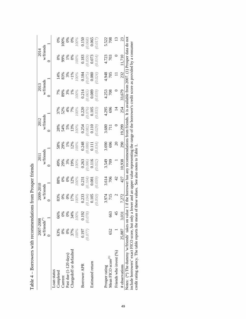
In Tables 3, 4 and 5 we split borrowers based on soft-type of information, such as being part
of a group or not (Table 3), having recommendations from other Prosper borrowers or not (Table
4), and having borrowed previously on Prosper or not (Table 5). Few interesting observations
25
emerge. First, before SEC registration, borrowers belonging to a group appear to be riskier (higher
FICO). Second, borrowers with friends pay lower rates.29 Last, borrowers with previous Prosper
loans (Table 5) appear to pay relatively lower rates in the most recent years covered by the sample
despite their FICO and Prosper ratings being not significantly higher than those of first-time
borrowers. Also, they exhibit fewer charged offs and defaults. This suggests that the availability
of a public credit history is important, even beyond the availability of soft signals, in reducing
information premia and lending rates. The longer the credit history is, the stronger the decline is.
4.4 Lending Rates, Hard and Soft Information Signals
In this section we start examining the selection and information channels previously rationalized
through our model. To this purpose we report regressions of lending rates on all types of available
signals (private signals, hard information and soft information) with the goal of testing the direc-
tion and the significance of their impact. As explained earlier, signals indicating a reduction in
borrowers’ risk might induce a decline of lending rates due to a selection effect (better borrowers’
quality and lower default rates) or due to an increase in information precision (investors can better
discern borrowers and require lower premia). In this section we will not identify separately those
two effects, but assess them jointly. We will distinguish the channels in the next section.
Before going forward it is important to mention that, given the change in the rate setting
procedure from an auction-type to a centralized system, in our analysis we always repeat estimation
splitting the sample based on the type of rate setting.
Tables 6 reports the results of OLS regressions of lending rates on loan characteristics (size,
term, motive), as reported by borrowers (private signals), and dummies for year-quarter of listing
and for borrower’s state of address. In the first column, where we pool all years, these variables
explain around 23 percent of lending rates’ variability.30 Noteworthy, when we split the sample,
based on regressions’ adjusted 2s, the explanatory power of the regressors is higher when Prosper
29This evidence is consistent with that of Lin, Prabhala, and Viswanathan [22] who focus on the likelihood of being
funded and find that friendships have a much larger impact than group membership.30The relationship between lending rates and size of the loan is U-shaped with a minimum at $4,700. Increasing
the term by 1 month raises the rate by 1 percentage point. Loans for debt consolidation and for business funding are
charged rates that are higher by half and one percentage point respectively. Similar results obtain when replacing
the left-hand-side variable with effective loan yields, or with Prosper ratings, estimated returns or estimated losses.
Regressions available upon request.
26
starts setting rates centrally.31 However, most heterogeneity remains unexplained. This confirms
our previous argument that a centralized pricing system, which more efficiently conditions on all
available signals, and a longer credit history increase information efficiency.
In the regressions in Table 7, we add variables capturing the public signals that lenders can
use to infer borrowers’ quality. In columns (1) to (3) we include only variables conveying hard
information, which consist of quantitative and verifiable signals, such as borrowers’ FICO score,
number of open credit lines, number of credit inquires, a dummy for any current delinquencies,
monthly income, and debt-to-income ratio. These variables improve substantially the ability of
the regression model to explain the variability of lending rates. The analysis suggests that loan
rates are decreasing in the FICO score: a one standard deviation (70 point) increase in the FICO
score lowers the lending rate by approximately 4 percentage points (20 percent of the mean rate).32
Being delinquent, having a large number of open credit lines and of credit inquiries, having a low
income, or a high debt to income ratio also increase rates.33
In the last three columns of table 7, we add in variables conveying additional information of
a softer type, i.e. whose value and bearing have a major subjective component. These consist of
dummies for participation in a group, for endorsement from Prosper friends with or without Prosper
friends’ investment, and for previous borrowing on the platform. In line with the implications of our
model regarding the impact of information and with the studies on the role of networks mentioned
earlier, once credit risk is controlled for, being part of a group lowers loan rates, by between half and
two percentage points. When it comes to friendships, we find that rates are lower for borrowers with
funding from friends (with or without recommendation) by up to 4.5 percentage points before 2009,
and by up to 1.5 percentage points after 2009.34 The decline in the significance of those soft signals
31Results are robust to pooling the data and interacting the regressors with a dummy that takes on value 1 if the
loan is funded when rates are set centrally, instead of splitting the sample. Also, the evidence is similar if we take as
available upon request.32 In our sample the FICO score ranges between 500 and 900. A FICO below 600 signals poor credit history. A
FICO above 750 signals an excellent history.33Being delinquent on some other account raises the rate by 1 to 3 percentage points. A monthly income higher
by one standard deviation ($8000) lowers the rate by 1 percentage point. Increasing the debt-to-income ratio by one
standard deviation raises the rate by up to 1.5 points.34 It is interesting to notice that if we omit credit risk measures from the regression, the coefficient of the group
membership dummy becomes significant and positive. This suggests an omitted variable bias and is consistent
with the hypothesis that group participation may facilitate funding of risky borrowers, which generates a positive
correlation between individual riskiness and group participation as Table 3 suggests.
27
might also be due to the decline in the incidence of group participation and of recommendations
as evident from table 2.35
Last, it is interesting to notice that social network variables are significant also in the regres-
sions on the sample of loans whose rates are set centrally, despite the fact that these variables
become visible only after the posting of the loan, hence after Prosper algorithm sets the interest.
This suggests that Prosper pricing algorithm is somehow capable of anticipating the information
content of these variables. This seemingly puzzling feature can be explained by examining the re-
gression in the last column of the table which includes a dummy for previous Prosper loans. In this
regression the dummy for group membership becomes negligible and statistically insignificant and
the coefficients of the dummies for recommendations and/or on investment from friends become
very small (some become outright insignificant). Instead, the dummy for previous borrowing on
the platform has a large, significant and negative coefficient, suggesting that returning borrowers
pay over four percentage points less than “new” borrowers, ceteris paribus. It is very plausible that
a positive correlation exists between joining a group and the number of Prosper friends, on the
one hand, and previous funding on the platform, on the other, and this is part of the information
stored in the centralized system.
4.5 Lending Rates and Signals: Identifying Selection versus Information Chan-
nel
In the previous section we have established that signals of various types have a significant impact on
lending rates. Generally speaking the availability of information suggesting relatively low borrowers’
risk reduces lending rates. As explained earlier, however, this decline might be due to either a
selection effect (higher borrower quality reduces default rates) or to an information channel (for
given borrowers’ quality, the more the information is, the better the investors are at discerning
borrowers). In this section we wish to quantify how much of the decline is due to the information
channel relatively to the selection channel.
Table 8 reports the results of OLS regressions where we quantify the role of information and
signal precision in reducing premia and lending rates. To construct a measure of signal precision
35All results are robust to running regressions on all listings and interacting the right-hand-side variables with
dummies for loans priced by Prosper and to introducing Prosper in-house credit rating measures in the regressions.
28
we exploit the variability in the type of information reporting among borrowers.
We consider first the case of income. From the regression in column (1) of table 7, borrowers
whose income is at the 75 percentile of the distribution pay 50 basis point less than borrowers
at the 25 percentile, ceteris paribus. Hence, borrowers with higher income levels pay lower rates
(selection effect). However beyond variability in income per se, there is also variability in the type
of reporting. In fact, most borrowers provide official documentation to support their statement, but
over 8 percent of the sample does not. This difference can proxy for signals’ precision. In column
1 of table 8, we augment the benchmark regression of table 7 with a dummy that takes on value 1
if the borrower income can be verified and with interactions of this dummy with income and with
the debt-to-income ratio. The dummy has a large, negative and statistically significant coefficient.
To get a sense of the magnitude of this effect, we can compare two borrowers with identical median
income and debt-to-income ratio but different reporting. The borrower that provides documentation
about his income pays over 1 percentage point less than the other, consistent with the hypothesis
that higher signal precision contributes in a statistically significant way to reduce lending rates.36
Next, we consider credit lines. In the regression in column (1) of table 7, this variable has
a positive and statistically significant coefficient. More credit lines are associated with more risk,
hence with higher lending rates (selection effect). However, about 1 percent of borrowers has no
credit lines open. Having no credit lines open cannot be associated with being more or less risky
because one could have no credit lines because she has never applied or because her applications have
been turned down. Instead, having some credit line open can help investors to discern borrowers’
quality (information channel). To verify this, in the regression reported in column 2, we replace
the number of credit lines with a dummy that takes on value 1 if the borrower has no credit lines
open (value 0 if she has any). The dummy has a positive, extremely large and significant coefficient
and implies that borrowers without any open credit line pay on average 2.4 percentage points more
than those who do have them. This result is important since it shows again that the information
channel is quantitatively very important. Interestingly, our results give a clear quantification of the
value of information in terms of how much returns investors are willing to give up in exchange of
an increase in its precision.
36Notice that strategic non-reporting of this information is not an issue in that what matters is the fact that for
some borrowers the available information is perceived as less reliable (whatever the reason).
29
Next, in the regression in column 3, we consider the state of residency which over 30 percent
of borrowers do not report before Prosper registered with the SEC.37 In this case we add a dummy
that takes on value 1 if the state of residency is missing. The absence of this piece of information, by
lowering the precision of the signals available, raises the average lending rate by almost 2 percentage
points. Last, in the fourth column of table 8, we consider the reasons for borrowing, which is missing
for about 10 percent of the loans posted after 2009. Similarly to the case of residency reporting,
we add a dummy to single them out. Lending rates appear to be higher (by over half percentage
points) for borrowers who omit this information.38
Overall, this evidence confirms that the information channel per se is quantitatively very
important in driving the decline in lending rates, hence in increasing market efficiency.
4.6 Lending Rates and Banking Fragility
Another important prediction of our model concerns the substitutability between different forms of
investment. In principle, markets and banks could be either substitutes or complements. If banks
eventually adopt a digital screening technology, competition between the two sectors might induce
complementarity. However, our empirical analysis, discussed below, suggests that substitution is
prevailing. This is also the reason why in our model we favoured assumptions inducing substitution.
Indeed, complementarity is more likely to emerge over time when the banking sector engages more
heavily into digital investment. Instead, so far, the narrative has been of a migration of investors
to the digital platform due to fears of fragility in the banking sector.
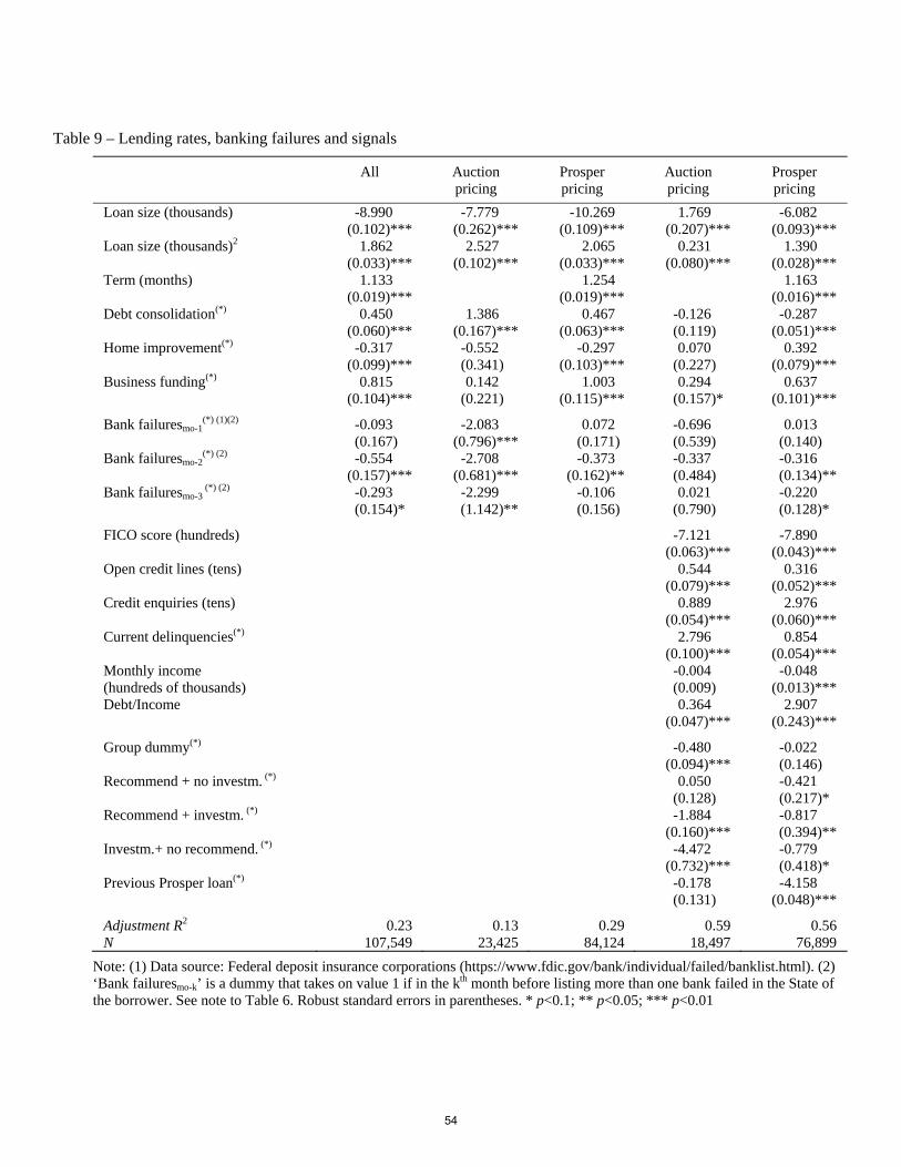
To investigate this issue we add to our regressions a proxy for bank fragility, based on in-
formation on bank failures as reported by the Federal Deposit Insurance Corporation. Over the
period considered, 497 bank failures were recorded in the US, with most occurring between 2009
and 2011. 42 states experienced at least one bank failure. We use these data to augment our
regressions with three dummies that take on value 1 if, in the borrower’s state, more than one
financial institution failed the month before, or two months before, or three months before the loan
37After SEC registration, information on the state is available for all borrowers.38The regressions testing the significance of non reporting the state of residency and the reason for borrowing use
observations that are dropped from the sample used for all other regressions. Including these observations in the
previous regressions does not affect the size and significance of the coefficients of the other variables of interest.38The Federal Deposit Insurance Corporation is the agency that is typically appointed as receiver for failed banks.
The original list includes all banks which have failed since October 1, 2000.
30
was funded. Notice that we have included in the regressions both year-quarter and state dummies
to capture other aggregate shocks. Results are in Table 9. The dummies’ coefficients are negative
and generally significant which suggests that, where significant rates of bank failures were recorded,
agents increasingly turned to the platform, increasing liquidity and hence inducing a decline in P2P
loan interests. The reduction in rates is between 20 and 30 basis points which is an admittedly
small effect, most likely due to the fact that we are restricting the availability of instruments that
are alternative to the banking sector. In practice, agents have more choices and asset substitution
might take place among different asset classes.
Nevertheless, overall, this evidence is consistent with our model prediction that when there are
signs of fragility in the banking system more borrowers and lenders turn to P2P platforms. This
leads to lower equilibrium rates which reflect not only higher demand and higher supply, but also
the presence of a larger share of good projects on the online market, with a reduction of information
premia.
4.7 Robustness - Lending Club
To fully assess the robustness of our results we have repeated the analysis using data from US
Lending Club, which is the world’s largest P2P lending platform. Loan application processes and
funding are very similar to Prosper. Specific institutional details and data description for this
platform are in Appendix 8.
Table 10 below reports the results of OLS regressions whose specifications parallel the ones
used with Prosper data. For ease of reading we report also the corresponding Prosper regressions
from tables 6, 7 and 9. Compared to Prosper, Lending Club data yield more precise estimates due
to higher sample size, but the evidence is very similar.
In the first column of table 10, we regress rates only on loan characteristics (size, term, motive)
and on dummies for quarter-year of listing and state of address of the borrower, which explain
38We have measured bank fragility also using the (state-invariant) average ratio of currency in the hands of public
to demand deposits in the year before the loan was posted. This variable reflects the idea that before the occurrence
of banking panics depositors demand a large scale transformation of deposits into currency. Gorton [16] shows
that historically the ratio of currency to demand deposits has indeed increased at panic dates. Consistent with the
predictions of our model, we find that the more currency the public held relative to deposits in the year before listing,
the lower the equilibrium rates. In other words, as the fragility of the banking sector increases, investors migrate to
the platform, which increases liquidity and lowers the rates. Regressions are available upon request.
31
around 29 percent of the variability of lending rates (23 percent in Prosper data regression, second
column). In the third column of the table, we add in variables capturing the signals that lenders
can use to infer borrowers’ quality. As explained earlier, Lending Club offers fewer indicators
compared to Prosper, because soft information is missing. As hard signals, we include dummies for
Lending Club credit grade (in the absence of borrowers’ FICO score), the number of open credit
lines and the number of credit inquires, a dummy for any delinquencies in the previous two years,
annual income, and the debt-to-income ratio. Like with Prosper data, these variables improve
enormously the ability of the regression model to explain the variability of lending rates. Also, the
analysis suggests that rates are lower the better the credit grade is, which is a clear indication of
the signalling role of those metrics. We also find that lending rates are higher the larger the number
of credit enquiries and of open credit lines. They are higher for borrowers who report delinquencies
on other loans, whose income is relatively low and their debt-to-income ratio is relatively high.
This is again all consistent with the fact that public signals facilitate convergence to a separating
equilibrium where lenders require higher loan spreads to fund riskier borrowers.
In columns 5 and 7 of the same table, we add to the regression the dummies for financial
institution failures in the state of residency of the borrower, one, two and three months before loan
funding which proxy for liquidity shortage and fragility risk in the banking sector. Consistent with
the predictions of our model regarding bank-platform substitutability, and in line with the evidence
from Prosper data, we find that borrowers living in states that experience financial institutions’
failures pay lower rates. Again, like in Prosper data regressions, the estimated effects are relatively
small possibly because we consider only bank deposits and P2P loans and do not allow for other
instruments which could be involved in the substitution.
5 Conclusions
P2P lending has experienced an impressive growth over the recent years and has penetrated most
markets including high growth economies like China. Despite the lack of delegated monitors,
and the potential costs of asymmetric information, data suggest that this new intermediation
service is performing well relatively to traditional banking39. Two are the main externalities that
39Recent speeches by policy makers (Constancio [13]) highlight its potential benefits even hinting at the risks that
it may pose for the profitability of the banking sector.
32
make this market attractive. The first are information externalities. Thanks to digital technology,
lending platforms can provide a large variety of costless public information signals that help improve
market transparency and facilitate price discovery in separating equilibria. Second, in times of
bank fragility, platforms provide a valuable substitute that improves risk-sharing for investors and
borrowers. We explore those two hypotheses through a theoretical and an empirical analysis, the
latter based on data from the two biggest lending platform in the US, namely Prosper and Lending
Club. Importantly, our empirical analysis allows us to quantify the value of information since we are
able to quantify the reduction in rates that investors are willing to accept in exchange of additional
signals.
Our results have several important implications. First, they show that transparency in debt
markets helps to improve its liquidity and efficiency. This has important policy implications.
Transparency is a prerequisite of equity markets, while debt markets are typically opaque. After the
recent financial crisis, which originated in debt markets, a debate surged on whether enforcing higher
transparency in debt market might help to improve stability and efficiency. Lending platforms
provide a good experiment in this sense. Second our results also speak on the importance of fostering
the emergence and growth of markets offering alternative funding and investment opportunities with
respect to the traditional banking sector. This argument is at the core of important policy debates
such as the one on the creation of a capital market union in Europe.
33
References
[1] Akerlof G.(1970). “The Market for lemons: Quality uncertainty and the market mechanism.”
Quarterly Journal of Economics, 84(3), pp. 488-500.
[2] Allen, F. and D. Gale, (1999). “Diversity of Opinion and Financing New Technologies.” Journal
of Financial Intermediation, 8, 68—89.
[3] Allen, F. and D. Gale, (2000). Comparing Financial Systems, MIT Press.
[4] Allen, F., S. Morris, and H. S. Shin, (2006). “Beauty Contests and Iterated Expectations in
Asset Markets.” Review of Financial Studies, 19(3): 719—52.
[5] Bachmann, A., Becker, A., Buerckner, D., Hilker, M., Kock, F., Lehmann, M., Tiburtius, P.
and B. Funk (2011). “Online Peer-to-Peer Lending — A Literature Review.” Journal of Internet
Banking and Commerce; Vol. 16(2).
[6] Bacchetta, P. and E. van Wincoop, (2008). “Higher Order Expectations in Asset Pricing.”
Journal of Money, Credit, and Banking, 40(5): 837—66.
[7] Banerjee, A. V., (1992). “A Simple Model of Herd Behavior.” Quarterly Journal of Eco-
nomics,107(3), 797—817.
[8] Besley, Timothy and Stephen Coate (1995) “Group Lending, Repayment Incentives and Social
Collateral.” Journal of Development Economics, Vol. 46, 1-18.
[9] Bikhchandani, S., D. Hirshleifer, and I. Welch, (1992). “A Theory of Fads, Fashion, Custom,
and Cultural Change as Informational Cascades.” Journal of Political Economy, 100(5), 992—
1026.
[10] Board of Governors of the Federal Reserve System (2016). Charge-Off and Delinquency Rates
on Loans and Leases at Commercial Banks. http://www.federalreserve.gov/releases/chargeoff/
(downloaded on Oct. 20, 2016).
[11] Bonfim, D. and J. Santos, (2017). “The importance of deposit insurance credibility.” AEA
Meetings.
34
[12] Chemla, G. and K. Tinn, (2018). “Learning through Crowd-funding.” Mimeo, Imperial College.
[13] Constancio, V. (2016). “Challenges for the European Banking Industry.” Speech delivered the
Conference on “European Banking Industry: what’s next?”, organized by the University of
Navarra.
[14] Duarte, J., S. Siegel and L. Young, (2012). “Trust and Credit: The Role of Appearance in
Peer-to-Peer Lending.” Review of Financial Studies, 25(8), 2455-2483.
[15] Fang, L. and J. Peress, (2009). “Media Coverage and the Cross-Section of Stock Returns.”
Journal of Finance, 64(5), 2023-2052.
[16] Gorton, G. (1988). “Banking Panics and Business Cycles.” Oxford Economic Papers, New
Series, vol. 40(4), 751-781.
[17] Gorton, G. and A. Metrick, (2009). “Securitized Banking and the Run on Repo.” NBER w.p.
15223.
[18] Iyer, R., Khwaja, A., Luttmer, E. and K. Shue (2015). “Screening Peers Softly: Inferring the
Quality of Small Borrowers.” Management Science, Vol. 62(6) pp. 1554 - 1577.
[19] Kaufmann, C., M. Weber, and E. Haisley, (2015). “The Role of Experience Sampling and
http://www.liberum.com/alternative-finance/opinion-insight (on October 17, 2016).
[22] Lin, M., Prabhala, N. and Viswanathan, S. (2013). “Judging Borrowers by the Company They
Keep: Friendship Networks and Information Asymmetry in Online Peer-to-Peer Lending.”
Management Science, Vol. 59(1), pp. 17-35.
[23] OECD (2015). Financing SMEs and entrepreneurs 2015. An OECD Scoreboard. OECD Pub-
lishing.
35
[24] Prime Meridian Capital Management (Accessed October 17, 2016 -
http://www.pmifunds.com/what-is-p2p-lending/).
[25] Paravisini, D., V. Rappoport and E. Ravina (2016). “Risk Aversion and Wealth: Evidence
from Person-to-Person Lending Portfolios.” Forthcoming Management Science.
[26] Peress, J. (2004). “Wealth, Information Acquisition and Portfolio Choice.” Review of Financial
Studies, 17(3), 879-914.
[27] Petriconi, S. (2016). “Bank Competition, Information Choice and Inefficient Lending Booms.”
Mimeo, Bocconi university.
[28] Ravina, E. (2012). “Love and Loans: The Effect of Beauty and Personal Characteristics in
Credit Markets.” Unpublished. Available at SSRN: http://ssrn.com/abstract=1101647.
[29] Repullo, R. and J. Suarez, (2013). “The Procyclical Effects of Bank Capital Regulation.”
Review of Financial Studies, vol. 26(2), pages 452-490.
[30] Ruckes, M. (2004). “Bank competition and credit standards.” The Review of Financial Studies,
17(4):1073-1102.
[31] Spence, M. (1973). “Job Market Signaling.” Quarterly Journal of Economics, Vol. 87(3), pp.
355-374.
[32] Stiglitz, J. and A. Weiss, (1981). “Credit Rationing in Markets with Incomplete Information.”
American Economic Review, 71(3), pp. 393-410.
[33] Theil, H. (1967). Economics and Information Theory, Rand McNally and Company - Chicago.
[34] Tinn, K. (2010). “Technology Adoption with Exit in Imperfectly Informed Equity Markets.”
American Economic Review, vol. 100(3), pages 925-57.
[35] Van Nieuwerburgh, S. and L. Veldkamp, (2010). “Information Acquisition and Under-
diversification.” Review of Economic Studies, 77(2), 779-805.
[36] Yaari, M. (1965). “Uncertain Lifetime, Life Insurance and the Theory of Consumer.” Review
of Economics Studies, 32, 137-50.
36
[37] Zopa.com (Accessed October 17, 2016 - https://www.zopa.com/about).
[38] Wette, H. (1983). “Collateral in Credit Rationing in Markets with Imperfect Information:
Note.” American Economic Review, vol. 73, issue 3, 442-45.
37
6 Appendix A. Simulated Model
In section 3, we have derived analytically and discussed the channels of transmission at work in
the model. Now, we quantify the effects through simulations that solve the entire set of equations
of the model simultaneously. We proceed by calibrating the model and simulating it subject to
a set of shocks. Specifically, we simulate the effects of shocks to the signal precision, to the
average success probability,− whereby shocks to the latter capture the selection channel through
first order stochastic changes in the distribution of projects, and to the aggregate project return,
Last, to capture the substitution channel, we shock the probability of bank default,
The impulse responses to those shocks allow us to rationalize further our data evidence through
graphics and through the lenses of a full model solution. The parameters of the model are chosen
as close as possible to their data equivalent. To add further realism to the quantitative simulations
we also estimated the shocks on data from US P2P platforms Prosper and Lending Club, and from
the banking system.
We start by detailing our parameter choice and shock estimation. We then present the impulse
response functions of selected variables and discuss the transmission mechanisms.
6.0.1 Calibration
Time is taken to be quarters. The discount factor, , is set to 0.99, so as to induce a risk-free
rate of 4% on annual basis. We assume a CRRA utility for households/lenders, 1−1− with a risk-
aversion parameter set to 2 which is within the range of most of the macro and household finance
literature. We experiment also with higher values and notice that the transmission of shocks is
robust. For the average haircut, Gorton and Metrick [17] report an average value of 17% for the
period 2007-2009 for the repo-haircut index, where repos are short-term debt, whose returns and
haircuts approximate well bank bonds’. We therefore set = 0940 and = 02 which yield an
average haircut,− of 18% on annual basis.
We then set the average probability of success so as to satisfy our condition ≥ − The return
is calibrated as follows. First, we set the value of using the banks’ break even condition,
40Bonfim and Santos[11] who examined severe bank run episodes in Europe find haircust at 9.9%. We use this
value as reference to calibrate
38
=+∼, and compatibly with an annual bank margin of 4% as in Repullo and Suarez[29].
Notice that monitoring costs are calibrated to 15 basis points on quarterly basis. This delivers a
value of = 12 (per quarter). The expected return of the P2P loans ish+ (1− )
−i . We
obtain a value for using condition (11) in the steady state. The latter depends upon the value of
. We shall set the benchmark value for so as to obtain an overall expected return on P2P loans
of 1.073 percent. This value is in line with those on Prosper and Lending Club loans. Specifically,
for Prosper, mean estimated returns range from 103% in 2009 to a value of 73% in 2014. The
equivalent in Lending Club are slightly lower.
As to the shocks, we model them as autoregressive processes. For the shock to the project
success probability, we take the loss rates of Lending Club loans for the period 2006 to 2016 and fit
an auto-regressive process. The estimation delivers a persistence of 0407039. Next, for the shock
to the return on banks’ liabilities,we collect quarterly data on the return on the equity of all U.S.
banks again for the period 2006 to 2016, and fit an auto-regressive process. This yields a persistence
of 0878877. We cannot calibrate the changes in the precision of signals directly, because in the data
it corresponds to a qualitative increase in transparency or in the number of the signals available.
Hence, for this shock, impulse responses are indicative of the qualitative trends in the transmission
mechanism. Last, to calibrate the liquidity shock we take the quarterly LIBOR-OIS spread from
Bloomberg (difference between the London interbank offered rate and the overnight swap index)
for the period 2006 to 2016 and again fit an AR(1) process. The resulting persistence is 0762562.
To conclude, notice that our model implies that households’ portfolio choice is between deposits
and P2P loans. To make sure that indeterminacy does not arise in steady state41 we guess a model-
consistent functional form for the aggregate wealth accumulation. This allows to pin down exactly
the investments in each asset.
6.0.2 Quantitative Results
Figure 1 shows the impulse responses of selected variables to a 1% increase in signal precision, .
This shock captures the information channel. An increase in (first panel) implies that investors
are now better at discerning loans’ quality. The threshold for the marginal funded project (second
41This possibility exists as different allocation between the two assets may be compatible with the same set of first
order conditions.
39
0 2 4 6 8 10 12 14 16 18 200
0.05
0.1
0.15
0.2
0.25Signal precision
0 2 4 6 8 10 12 14 16 18 20−2
−1.5
−1
−0.5
0Signal threshold
0 2 4 6 8 10 12 14 16 18 20−2.5
−2
−1.5
−1
−0.5
0P2P Information spreads
Figure 1: Impulse responses of selected variables to a 1% increase to signal precision .
panel) drops and households are willing to fund more projects. We also compute, and show in
the third panel, the average information spread, defined as the difference between the conditional
expected returnsh+ (1− )
−i under full information, namely with = 1 and under partial
information42. As expected, it also declines because the severity of the information asymmetry is
reduced.
Figure 2 shows the impulse responses to an increase in the average loan quality,− This rep-
resents a shift upward toward a probability distribution which first-order stochastically dominates
the initial one. Intuitively, the quality of all projects increases, for given signal precision. Hence,
this shocks captures purely the selection channel. An increase in− (first panel) results in a decline
of the threshold for the marginally funded project (because the average projects’ default rate has
declined) and also of the loan information spread, for any degree of signal precision. Like before,
households are now willing to fund more projects on the platform.
Figure 3 shows the impulse responses to an increase in projects’ return, Responses are
rather intuitive. Now. the expected return on the platform raises, and, hence, the loan spreads
42Note that this is different, albeit related to the individual loan spreads, =1() − () described in the
analytical section 3.3.
40
0 2 4 6 8 10 12 14 16 18 200
0.1
0.2
0.3
0.4
0.5Average success probability
0 2 4 6 8 10 12 14 16 18 20−2
−1.5
−1
−0.5
0Signal threshold
0 2 4 6 8 10 12 14 16 18 20−2.5
−2
−1.5
−1
−0.5
0P2P Information spreads
Figure 2: Impulse responses of selected variables to a 1% increase to average sucess probability,−
requested by households fall. The threshold for the marginal projects falls too and households fund
more projects.
Finally, figure 4 shows the impulse responses to changes in the probability of bank defaults.
This simulation is meant to capture the substitution channel. For this reason, in this case, we
plot the returns on deposits and the return on the P2P loan funded at the margin. As risk in the
banking sector raises, banks have to offer higher returns to depositors. Still savings shift to the
relatively less risky P2P sector and this reduces the marginal return there.
7 Appendix B. Prosper Data Description
Prosper (http://prosper.com) is an online platform for peer-to-peer lending, which opened up on
February 5th, 2006, in the US. Borrowers create personal profiles and solicit loans via online
listings detailing the amount requested, the interest rate, the term and purpose for the loan. The
borrower’s profile includes independently verified information on his credit history43, income, and
43Each listing includes hard credit data such as lower and upper values delimiting the range of the borrower’s credit
score as provided by a consumer credit rating agency, number of credit inquiries in the last six months, the number
of open credit lines, revolving accounts and credit account records, and number of accounts delinquent.
41
0 2 4 6 8 10 12 14 16 18 200
0.5
1
1.5Aggregate project return
0 2 4 6 8 10 12 14 16 18 20−5
−4
−3
−2
−1
0Signal threshold
0 2 4 6 8 10 12 14 16 18 20−2.5
−2
−1.5
−1
−0.5
0P2P Information spreads
Figure 3: Impulse responses of selected variables to a 1% increase to aggregate project return,
0 2 4 6 8 10 12 14 16 18 200
0.05
0.1
0.15
0.2Probability of bank defaults
0 2 4 6 8 10 12 14 16 18 200
0.5
1
1.5
2Deposit return
0 2 4 6 8 10 12 14 16 18 20−0.06
−0.04
−0.02
0
0.02Marginal P2P return
Figure 4: Impulse responses of selected variables to a 1% increase to probability of bank default,
42
current debts. Each listing includes also a Prosper Rating, i.e a credit grade that goes from 7 (label
AA) to 1 (label HR - "High Risk") determined by Prosper based on a proprietary algorithm. This
rating depends on two scores: (1) the credit score, obtained from an official credit reporting agency,
and (2) Prosper Score, computed in-house based on the Prosper population.44
Prosper also creates social networks by linking borrowers in groups (tied by geography, com-
mon interest, or common loan purpose) and collecting the endorsements of other Prosper members
(friends). For what concerns groups, any borrower can join one of the several groups in the Pros-
per marketplace or propose one. There are groups related to a school (alumni) or an employer,
geographically-oriented groups, military groups, medical groups related to medical reasons for bor-
rowing, demographic groups highlighting some particular demographics, such as single parents or
Hispanics, groups targeting people with particular hobbies, religiously-oriented groups, and busi-
ness groups for small businesses, or for new business development. Admission to a group is based
on eligibility criteria. Some groups, such as employee or university alumni groups, require veri-
fication of the qualifying criteria, whereas others have looser joining criteria. An individual can
be a member of only one group at a time and borrowers cannot leave or change group until loan
repayment.
In turn, lenders assess and can bid on listings. The minimum bid is set at $25. At its incept
Prosper operated a variable rate model. It worked as an eBay-style auction marketplace. In their
bid, lenders would specify the investment and the minimum interest they were willing to accept.
If the total bid amount exceeded the amount requested, those lenders asking the lowest interests
were granted a share of the loan. In 2009, Prosper registered with the SEC and afterwards it
changed its business model to use pre-set rates determined solely by an own algorithm evaluating
each prospective borrower’s profile and credit risk. Under the new approach, lenders no longer
determine the loan rate in an auction. Instead, they simply choose whether or not to invest at
the rate which Prosper’s loan proprietary pricing algorithm assigns to the loan after analyzing the
borrower’s credit report and financial information. Following the SEC registration, new prospective
borrowers are required to have a FICO credit score of at least 640, while returning borrowers only
need a score of 600 to request a loan.45
44Prosper Ratings are available for loans originated after July 2009.45The original model effectively had the investors setting the rates through an open bidding process. The problem
43
Borrowers are limited to a maximum of two concurrent loans of $25,000 or less each until
2012, $35,000 thereafter.46 Fees of 1 to 5 percent of the loan amount are deducted from the loan,
depending on the borrower’s risk profile and loan duration. Loans amortize over a 36-month period
until 2009, a maximum 60-month period thereafter. Repayments are in monthly installments that
are automatically deducted from a borrower’s bank account. Prosper loan status is defined as
‘Completed’ if the loan has been fully paid off, and as ‘Current’ if payments are made on time
and as agreed. When the borrower misses payments, loans are classified as ‘Past due’. When
loans are 120 days past due (i.e., 4 payments are missing), Prosper moves them to ‘Charged off’
status. A loan designated as ‘Charged off’ is due in full immediately. It can also be sold to outside
debt collectors. For investors, the entire balance moves into a charged off balance and is assumed
to be lost. There are some cases where, after a loan is charged off, the borrower may still make
some payments. About 16% of Prosper’s charged off loans have had some level of recovery. A
loan is tagged as in ‘Default’ in case of delinquency, bankruptcy or death. Bankruptcy is the most
prominent reason for a loan to be tagged as defaulted. Some of the loans in ‘Default’ ultimately
get settled or paid in part or in full. Delinquencies are reported to credit report agencies and affect
the borrower’s credit score. Borrowers who default on their loans are not allowed to borrow using
Prosper.com again.
8 Appendix C. Lending Club Institutional Data Description
Lending Club is the world largest platform for peer-to-peer lending. All loans are unsecured personal
loans and are between $1,000 and $35,000. Based on the borrower’s credit history and score, on her
debt-to-income ratio and desired loan amount, Lending Club assigns loans a letter credit grade to
which a specific interest rate and fees are associated. Rates vary between 5% and 26% depending
on the credit grade. The range of grades is similar to Prosper’s, but Prosper’s average interests
with that original model, that was shut down by regulatory authorities, is that the investors were individuals without
any demonstrable skill and there were no controls in place to ensure that they had sufficient resources to take on the
risk. Additionally, that model had severe inefficiencies because of a lack of large institutional investors that could
immediately fund a whole loan. This left severe cash drag issues with many loans going unfunded. Additionally, from
a regulatory perspective, there were severe lending risks due to no discernible way in which the interest rates were
set.46Currently, loans are funded if they obtain 70 percent or more of the amount requested. Originally, no partial
funding was allowed.
44
are higher. For example, for credit grade A, the rate is 4% higher, and that difference increases as
credit grade worsens. The standard loan period is three years. A five year period is available at a
higher interest rate and additional fees. Loans can be repaid in full at any time without penalty.
Investors can search and browse the loan listings on Lending Club website. The minimum
investment is $25.
Lending Club makes money by charging borrowers an origination fee, which ranges between
1% and 5% depending on the credit grade, and charging lenders a 1% service fee on all amounts
the borrower pays. To reduce default risk, Lending Club focuses on high creditworthy borrowers,
with a FICO score of 660 or more, declining approximately 90% of the loan applications as of 2012.
Summary statistics for this data set are in tables C1 and C2. Most borrowers on Lending
Club’s website report using their loans to refinance other loans or pay credit card debt (table C1,
panel (a)). Like for Prosper, the share of this type of borrowers has increased over time, whereas
the share who intend to fund their business has sharply declined. Borrowers debt-to-income ratio
(excluding mortgage) has increased over time and gone from 10 percent in 2007 to 18 percent in
2014 (table C2). On average, borrowers have 11 open credit lines; 20 percent have been delinquent
on a loan in the two years before borrowing on Lending Club. The mean personal income is $73,000
and the average loan is $14,000. Investors funded $5 mln in loans in 2007 up to $3.5 bln in 2014.
The nominal average interest rate was 12% in 2007 and 14% in 2014. The default rate is around
11%.
45
Tabl
e 1
– Su
mm
ary
Stat
istic
s
Pane
l (a)
Y
ear o
f the
loan
20
0620
0720
0820
0920
10
2011
2012
2013
2014
Bor
row
er le
ndin
g ra
te
0.19
10.
177
0.18
60.
193
0.21
3 0.
230
0.22
00.
184
0.15
3(0
.069
)(0
.064
)(0
.085
)(0
.091
)(0
.098
) (0
.079
)(0
.077
)(0
.061
)(0
.054
)B
orro
wer
ann
ual p
erce
ntag
e ra
te (A
PR)
0.20
10.
186
0.20
40.
216
0.23
9 0.
262
0.25
30.
214
0.18
2
(0.0
70)
(0.0
66)
(0.0
89)
(0.0
95)
(0.1
06)
(0.0
86)
(0.0
82)
(0.0
65)
(0.0
59)
Estim
ated
eff
ectiv
e yi
eld
0.
103
0.10
6 0.
213
0.20
10.
162
0.13
4
(0.0
52)
(0.0
55)
(0.0
74)
(0.0
71)
(0.0
54)
(0.0
48)
Size
of l
oans
47
6370
5060
2243
5547
67
6692
7834
1054
511
912
(440
4)(6
126)
(540
0)(4
070)
(371
4)
(427
3)(5
527)
(657
5)(6
684)
Term
(mon
ths)
36
3636
3636
37
4345
44
Ti
me
for f
undi
ng (m
edia
n)
911
1014
12
108
65
Lend
ers’
inve
stm
ent:
mea
n/m
edia
n 23
1/96
126/
5812
2/45
98/2
955
/35
286/
7838
1/89
5,76
2/3,
000
9,13
1/9,
000
No.
of i
nves
tors
: mea
n/m
edia
n 57
/36
127/
9213
6/95
146/
9313
4/10
3 80
/55
82/5
356
/129
/1Lo
ans f
unde
d by
sing
le in
vest
or (%
) 2
11
1<1
1
251
75
Lo
ans f
or d
ebt c
onso
lidat
ion
(%)
4246
4748
48
7479
42
hom
e im
prov
emen
t (%
) 5
910
11
116
45
b
usin
ess (
%)
1611
1011
9
43
16
oth
er (%
) 37
3433
30
3216
1437
# ob
serv
atio
ns
5,90
611
,460
11,5
522,
047(1
)5,
652
11,2
2819
,553
33,9
1011
,734
(2)
Not
es: M
ean
valu
es, u
nles
s spe
cifie
d ot
herw
ise.
Sta
ndar
d de
viat
ions
in p
aren
thes
es. (
1) In
200
9, lo
an is
suan
ce w
as su
spen
ded
durin
g Pr
ospe
r reg
istra
tion
with
th
e SE
C. (
2) Lo
ans i
ssue
d fr
om Ja
nuar
y to
Mar
ch 1
1th.
Pane
l (b)
– L
oan
stat
us (a
s of M
arch
31st
201
4)
Yea
r of t
he lo
an
2006
20
07
2008
20
09
2010
20
11
2012
20
13
2014
To
tal
Com
plet
ed
61%
61
%
67%
85
%
83%
49
%
28%
7%
1%
34
%
Cur
rent
-
- -
- -
29%
54
%
89%
99
%
49%
Pa
st D
ue (1
-120
day
s)
- -
- -
- 3%
4%
3%
-
2%
Cha
rged
-off
16
%
26%
24
%
11%
14
%
16%
12
%
1%
- 11
%
Def
aulte
d 23
%
14%
9%
4%
3%
3%
2%
0%
-
4%
100%
10
0%
100%
10
0%
100%
10
0%
100%
10
0%
100%
10
0%
46
Tabl
e 2
– H
ard
and
soft
info
rmat
ion
abou
t bor
row
ers
Yea
r of t
he lo
an
2006
20
07
2008
20
09
2010
20
11
2012
20
13
2014
M
ean
FIC
O sc
ore(1
) 60
9 65
4 67
4 71
5 71
4 70
9 71
1 70
8 70
3 N
umbe
r of o
pen
cred
it lin
es
8
8 9
8 8
8 10
11
(5
) (5
) (5
) (5
) (5
) (5
) (5
) (5
) N
umbe
r of c
redi
t inq
uirie
s
11
10
8
6 4
4 4
4 4
(1
2)
(11)
(8
) (5
) (4
) (4
) (4
) (4
) (4
) B
orro
wer
s w/ c
urre
nt d
elin
quen
cies
(%)
52
39
23
11
14
21
20
15
10
Pr
ospe
r cre
dit r
atin
g 4.
286
3.83
7 3.
552
3.68
8 4.
258
4.71
8 (1
.937
) (1
.985
) (1
.710
) (1
.829
) (1
.468
) (1
.387
) Es
timat
ed lo
ss
0.
075
0.09
3 0.
097
0.09
1 0.
073
0.06
2 Es
timat
ed re
turn
at i
ssua
nce
0.
103
0.10
3 0.
115
0.11
0 0.
088
0.07
3
D
ebt-i
ncom
e ra
tio
0.24
9 0.
431
0.25
4 0.
228
0.23
0 0.
251
0.26
4 0.
264
0.25
9
(0.7
37)
(1.3
18)
(0.3
42)
(0.1
52)
(0.2
99)
(0.4
02)
(0.4
64)
(0.2
43)
(0.1
13)
Mon
thly
inco
me
4,74
4 4,
654
4,61
9 5,
092
5,29
1 5,
660
5,71
0 6,
161
6,33
6
(5,2
07)
(4,7
11)
(3,7
05)
(3,2
25)
(4,0
99)
(8,5
44)
(13,
350)
(5
,664
) (4
,382
) B
orro
wer
s who
are
in a
gro
up (%
) 70
51
14
11
9
5 3
1 1
Bor
row
ers w
ith re
com
m. f
rom
Pro
sper
frie
nds (
%)
17
18
8 6
3 2
1 <1
B
orro
wer
s with
inve
st. f
rom
Pro
sper
frie
nds (
%)
6 7
5 4
1 1
<1
<1
$ in
vest
men
t fro
m fr
iend
s (co
nd. o
n ha
ving
frie
nds)
93
9 10
17
713
773
572
429
233
298
Bor
row
ers w
ith p
revi
ous P
rosp
er lo
ans (
%)
- 4
15
43
34
34
28
19
10
# ob
serv
atio
ns
5,90
6 11
,460
11
,552
2,
047
5,65
2 11
,228
19
,553
33
,910
11
,734
N
otes
: (1)
Pros
per d
ata
do n
ot in
clud
e bo
rrow
ers’
exa
ct F
ICO
scor
e, b
ut o
nly
a lo
wer
and
an
uppe
r val
ue re
pres
entin
g th
e ra
nge
of th
e bo
rrow
er's
cred
it sc
ore
as
prov
ided
by
a co
nsum
er c
redi
t rat
ing
agen
cy. T
he ta
ble
repo
rts th
e m
ean
of th
ese
valu
es. S
ee a
lso
note
s to
Tabl
e 1.
47
Tabl
e 3
– B
orro
wer
s who
are
par
t of a
gro
up
20
06-2
008
2009
-201
0 20
11
2012
20
13
2014
In g
roup
In
gro
up
In g
roup
In
gro
up
In g
roup
In
gro
up
0 1
0 1
0 1
0 1
0 1
0 1
Loan
stat
us
Com
plet
ed
66%
58
%
83%
87
%
49%
56
%
28%
33
%
7%
11%
1%
1%
C
urre
nt
0%
0%
0%
0%
29%
26
%
54%
53
%
90%
84
%
99%
99
%
Past
due
(1-1
20 d
ays)
0%
0%
0%
0%
3%
2%
4%
4%
3%
3%
0%
0%
C
harg
ed o
ff o
r def
aulte
d34
%
42%
17
%
13%
19
%
16%
14
%
10%
1%
1%
0%
0%
10
0%
100%
10
0%
100%
10
0%
100%
10
0%
100%
10
0%
100%
10
0%
100%
B
orro
wer
APR
0.
193
0.20
1 0.
232
0.24
4 0.
263
0.25
2 0.
254
0.22
6 0.
214
0.19
1 0.
183
0.16
1
(0.0
81)
(0.0
71)
(0.1
04)
(0.1
02)
(0.0
86)
(0.0
89)
(0.8
18)
(0.0
80)
(0.0
65)
(0.0
75)
(0.0
59)
(0.0
64)
Estim
ated
retu
rn
0.10
5 0.
092
0.11
6 0.
111
0.11
0 0.
105
0.08
9 0.
083
0.07
3 0.
068
(0.0
50)
(0.0
60)
(0.0
32)
(0.0
34)
(0.0
29)
(0.0
31)
(0.0
19)
(0.0
23)
(0.0
14)
(0.0
16)
Pros
per r
atin
g
4.
010
3.42
9 3.
550
3.59
8 3.
676
4.17
9 4.
251
4.79
9 4.
722
5.20
9 M
ean
FIC
O sc
ore(1
) 66
9 62
7 71
6 69
9 71
0 69
7 71
2 69
5 70
9 70
2 70
3 70
2 Ti
me
for f
undi
ng
(med
ian)
10
11
12
13
10
9
8 7
6 7
5 6
# ob
serv
atio
ns
17,2
52
11,6
66
6,95
3 74
6 10
,676
55
2 19
,066
48
7 33
,499
412
11,6
6667
N
otes
: (1)
Pro
sper
dat
a do
not
incl
ude
borr
ower
s’ e
xact
FIC
O sc
ore,
but
onl
y a
low
er a
nd a
n up
per v
alue
repr
esen
ting
the
rang
e of
the
borr
ower
's cr
edit
scor
e as
pr
ovid
ed b
y a
cons
umer
cre
dit r
atin
g ag
ency
. The
tabl
e re
ports
the
mea
n of
thes
e va
lues
. See
als
o no
tes t
o Ta
ble
1.
48
Tabl
e 4
– B
orro
wer
s with
reco
mm
enda
tions
from
Pro
sper
frie
nds
20
07-2
008
2009
-201
0 20
11
2012
20
13
2014
w/fr
iend
s(*)
w/fr
iend
s w
/frie
nds
w/fr
iend
s w
/frie
nds
w/fr
iend
s 0
1 0
1 0
1 0
1 0
1 0
1 Lo
an st
atus
C
ompl
eted
63
%
66%
83
%
88%
49
%
58%
28
%
37%
7%
14
%
0%
0%
Cur
rent
0%
0%
0%
0%
29
%
29%
54
%
52%
89
%
83%
99
%
100%
Pa
st d
ue (1
-120
day
s)
0%
0%
0%
0%
3%
1%
5%
4%
3%
3%
1%
0%
Cha
rged
off o
r def
aulte
d 37
%
34%
17
%
12%
19
%
12%
13
%
7%
1%
<1%
0%
0%
10
0%
100%
10
0%
100%
10
0%
100%
10
0%
100%
10
0%
100%
10
0%
100%
B
orro
wer
APR
0.
197
0.19
2 0.
233
0.23
1 0.
263
0.24
8 0.
254
0.22
0 0.
214
0.18
4 0.
183
0.15
0
(0.0
77)
(0.0
78)
(0.1
04)
(0.1
04)
(0.0
86)
(0.0
88)
(0.0
82)
(0.0
76)
(0.0
65)
(0.0
75)
(0.0
59)
(0.0
68)
Estim
ated
retu
rn
0.10
5 0.
081
0.11
6 0.
111
0.11
0 0.
105
0.08
9 0.
080
0.07
3 0.
065
(0.0
50)
(0.0
59)
(0.0
32)
(0.0
34)
(0.0
29)
(0.0
33)
(0.0
19)
(0.0
24)
(0.0
14)
(0.0
17)
Pr
ospe
r rat
ing
3.97
4 3.
614
3.54
9 3.
690
3.68
0 4.
295
4.25
3 4.
948
4.72
3 5.
522
Mea
n FI
CO
scor
e(1)
652
663
715
706
709
696
711
696
708
705
703
708
Frie
nds w
ho in
vest
(%)
1 45
2
42
1 20
0
14
0 11
0
13
# ob
serv
atio
ns
25,8
87
3,03
1 7,
272
427
10,9
38
290
19,2
99
254
33,6
79
232
11,7
10
23
Not
es:
(*) T
he d
umm
y 'w
/frie
nds'
take
s on
valu
e 1
if th
e bo
rrow
er h
as a
ny re
com
men
datio
ns fr
om fr
iend
s. It
is a
vaila
ble
from
200
7. (1
) Pro
sper
dat
a do
not
in
clud
e bo
rrow
ers’
exa
ct F
ICO
scor
e, b
ut o
nly
a lo
wer
and
an
uppe
r val
ue re
pres
entin
g th
e ra
nge
of th
e bo
rrow
er's
cred
it sc
ore
as p
rovi
ded
by a
con
sum
er
cred
it ra
ting
agen
cy. T
he ta
ble
repo
rts th
e m
ean
of th
ese
valu
es.
See
also
not
es to
Tab
le 1
.
49
Tabl
e 5
– B
orro
wer
s with
pre
viou
s loa
ns th
roug
h Pr
ospe
r
2007
-200
8 20
09-2
010
2011
20
12
2013
20
14
Pr
ior l
oans
(*)
Prio
r loa
ns
Prio
r loa
ns
Prio
r loa
ns
Prio
r loa
ns
Prio
r loa
ns
0 1
0 1
0 1
0 1
0 1
0 1
Loan
stat
us
Com
plet
ed
63%
69
%
82%
86
%
49%
50
%
28%
30
%
6%
10%
1%
1%
C
urre
nt
0%
0%
0%
0%
27%
32
%
54%
53
%
91%
85
%
99%
99
%
Past
due
(1-1
20 d
ays)
0%
0%
0%
0%
3%
3%
4%
5%
3%
3%
0%
0%
C
harg
edof
f or d
efau
lted
37%
31
%
18%
14
%
21%
15
%
14%
12
%
1%
2%
0%
0%
100%
10
0%
100%
10
0%
100%
10
0%
100%
10
0%
100%
10
0%
100%
10
0%
Bor
row
er A
PR
0.19
4 0.
203
0.22
4 0.
249
0.27
1 0.
245
0.26
3 0.
227
0.21
8 0.
199
0.18
5 0.
171
(0
.078
) (0
.086
) (0
.103
) (0
.103
) (0
.086
) (0
.085
) (0
.082
) (0
.075
) (0
.063
) (0
.071
) (0
.059
) (0
.058
) Es
timat
ed re
turn
0.
107
0.09
7 0.
117
0.11
1 0.
111
0.10
7 0.
089
0.08
6 0.
073
0.07
0
(0
.047
) (0
.056
) (0
.032
) (0
.032
) (0
.029
) (0
.028
) (0
.018
) (0
.022
) (0
.014
) (0
.014
)
Pros
per r
atin
g
4.
255
3.42
4 3.
458
3.73
1 3.
502
4.17
8 4.
163
4.65
8 4.
697
4.97
3 M
ean
FIC
O sc
ore(1
) 66
4 66
5 72
5 69
7 71
8 69
3 71
9 68
9 71
0 70
3 70
3 70
2 #
obse
rvat
ions
26
,700
2,
218
4,98
5 2,
804
7,36
1 3,
867
14,1
65
5,38
8 27
,444
6,
466
10,5
56
1,17
7 N
otes
: (*
) The
dum
my
‘Prio
r loa
ns' t
akes
on
valu
e 1
if th
e bo
rrow
er fu
nded
som
e pr
ojec
t on
Pros
per b
efor
e. (1
) Pro
sper
dat
a do
not
incl
ude
borr
ower
s’
exac
t FIC
O sc
ore,
but
onl
y a
low
er a
nd a
n up
per v
alue
repr
esen
ting
the
rang
e of
the
borr
ower
's cr
edit
scor
e as
pro
vide
d by
a c
onsu
mer
cre
dit r
atin
g ag
ency
. Th
e ta
ble
repo
rts th
e m
ean
of th
ese
valu
es.
See
also
not
es to
Tab
le 1
.
50
Table 6 – OLS regressions of lending rates on loan characteristics
Note: The left-hand-side variable is the lending rate in percentage points. Quarter-year dummies and US state dummies are also included. (*) denotes a dummy variable. (1) ‘Auction pricing’ refers to loans whose rates are set by lenders, which was Prosper pricing mechanism until 2010. ‘Prosper pricing’ refers to loans whose rates are set centrally by Prosper before posting. (2) Until 2010, all loans had a 36 month term. Robust standard errors in parentheses. * p<0.1; ** p<0.05; *** p<0.01
51
Tabl
e 7
– O
LS re
gres
sion
s of l
endi
ng ra
tes o
n lo
an c
hara
cter
istic
s and
sign
als
A
ll A
uctio
n pr
icin
g Pr
ospe
r pr
icin
g A
uctio
n pr
icin
g Pr
ospe
r pr
icin
g Pr
ospe
r pr
icin
g Lo
an si
ze (t
hous
ands
) -4
.336
1.
640
-6.3
31
1.76
6 -6
.292
-6
.082
(0.0
91)*
**
(0.2
08)*
**
(0.0
99)*
**
(0.2
07)*
**
(0.0
99)*
**
(0.0
93)*
**
Loan
size
(tho
usan
ds)2
1.03
7 0.
260
1.48
5 0.
234
1.47
8 1.
390
(0
.028
)***
(0
.081
)***
(0
.029
)***
(0
.080
)***
(0
.029
)***
(0
.028
)***
Te
rm
0.94
1
1.10
8
1.10
5 1.
162
(0
.017
)***
(0.0
17)*
**
(0
.017
)***
(0
.016
)***
D
ebt c
onso
lidat
ion(*
) -0
.231
-0
.098
-0
.130
-0
.120
-0
.125
-0
.287
(0.0
51)*
**
(0.1
20)
(0.0
55)*
* (0
.119
) (0
.055
)**
(0.0
51)*
**
Hom
e im
prov
emen
t(*)
0.04
0 0.
090
0.02
1 0.
057
0.04
3 0.
392
(0
.082
) (0
.227
) (0
.086
) (0
.227
) (0
.085
) (0
.079
)***
B
usin
ess f
undi
ng(*
) 0.
605
0.31
6 0.
508
0.29
7 0.
560
0.63
5
(0.0
94)*
**
(0.1
58)*
* (0
.108
)***
(0
.157
)*
(0.1
08)*
**
(0.1
01)*
**
FIC
O sc
ore
(hun
dred
s)
-7.0
11
-7.0
57
-7.2
95
-7.1
23
-7.3
42
-7.8
90
(0
.039
)***
(0
.063
)***
(0
.046
)***
(0
.063
)***
(0
.046
)***
(0
.043
)***
O
pen
cred
it lin
es (t
ens)
0.
329
0.52
4 0.
060
0.53
9 0.
074
0.31
4
(0.0
47)*
**
(0.0
80)*
**
(0.0
55)
(0.0
79)*
**
(0.0
55)
(0.0
52)*
**
Cre
dit e
nqui
ries (
tens
) 1.
658
0.89
4 2.
413
0.88
7 2.
454
2.97
7
(0.0
49)*
**
(0.0
55)*
**
(0.0
61)*
**
(0.0
54)*
**
(0.0
61)*
**
(0.0
60)*
**
Cur
rent
del
inqu
enci
es(*
) 1.
152
2.73
3 0.
833
2.79
7 0.
867
0.85
6
(0.0
51)*
**
(0.1
01)*
**
(0.0
57)*
**
(0.1
00)*
**
(0.0
57)*
**
(0.0
54)*
**
Mon
thly
inco
me
-0
.059
-0
.001
-0
.052
-0
.005
-0
.053
-0
.048
(th
ousa
nds)
(0
.015
)***
(0
.009
) (0
.015
)***
(0
.009
) (0
.015
)***
(0
.013
)***
D
ebt/I
ncom
e 1.
197
0.32
6 2.
742
0.36
4 2.
738
2.90
7
(0.0
75)*
**
(0.0
48)*
**
(0.2
28)*
**
(0.0
47)*
**
(0.2
29)*
**
(0.2
43)*
**
Gro
up d
umm
y(*)
-0
.512
-1
.938
-0
.026
(0
.092
)***
(0
.148
)***
(0
.146
) R
ecom
men
d +
no in
vest
m. (*
)
0.03
9 -2
.493
-0
.420
(0
.128
) (0
.222
)***
(0
.217
)*
Rec
omm
end
+ in
vest
m. (*
)
-1.8
84
-1.4
66
-0.8
38
(0.1
60)*
**
(0.4
11)*
**
(0.3
95)*
* In
vest
m.+
no
reco
mm
end.
(*)
-4
.478
-1
.198
-0
.809
(0
.732
)***
(0
.423
)***
(0
.419
)*
Prev
ious
Pro
sper
loan
(*)
-4
.158
(0
.048
)***
Adju
stm
ent R
2 0.
49
0.59
0.
51
0.59
0.
51
0.56
N
95
,396
18
,497
76
,899
18
,497
76
,899
76
,899
N
ote:
See
not
e to
Tab
le 6
. Rob
ust s
tand
ard
erro
rs in
par
enth
eses
. * p
<0.1
; **
p<0.
05; *
** p
<0.0
1
52
Ta
ble
8 –
Lend
ing
rate
s and
sign
al p
reci
sion
In
com
e ha
s bee
n ve
rifie
d N
o op
en c
redi
t lin
es
No
stat
e of
re
side
ncy
No
reas
on fo
r bo
rrow
ing
A
ll A
ll A
uctio
n pr
icin
g Pr
ospe
r pric
ing
Loan
size
(tho
usan
ds)
-4.3
76
-4.2
63
1.80
6 -6
.341
(0.0
90)*
**
(0.0
91)*
**
(0.1
96)*
**
(0.0
99)*
**
Loan
size
(tho
usan
ds)2
1.04
9 1.
015
0.18
3 1.
486
(0
.028
)***
(0
.028
)***
(0
.076
)**
(0.0
29)*
**
Term
0.
947
0.94
2
1.10
9
(0.0
17)*
**
(0.0
17)*
**
(0
.017
)***
In
com
e is
ver
ifiab
le(*
) -2
.406
(0
.925
)***
No
open
cre
dit l
ines
2.43
6
(0
.274
)***
N
o U
S St
ate(
*)
1.36
0
(0
.703
)*
N
o re
ason
for b
orro
win
g(*)
0.
630
(0.0
91)*
**
FIC
O sc
ore
(hun
dred
s)
-6.9
89
-6.9
62
-6.9
97
-7.2
96
(0
.039
)***
(0
.039
)***
(0
.059
)***
(0
.046
)***
O
pen
cred
it lin
es (t
ens)
0.
225
0.
480
0.06
0
(0.0
48)*
**
(0
.076
)***
(0
.055
) C
redi
t enq
uirie
s (te
ns)
1.67
5 1.
731
0.83
8 2.
416
(0
.048
)***
(0
.049
)***
(0
.051
)***
(0
.061
)***
C
urre
nt d
elin
quen
cies
(*)
1.15
4 1.
094
2.59
4 0.
832
(0
.051
)***
(0
.051
)***
(0
.094
)***
(0
.057
)***
M
onth
ly in
com
e (th
ousa
nds)
-0
.205
-0
.053
-0
.002
-0
.052
(0.0
69)*
**
(0.0
13)*
**
(0.0
08)
(0.0
15)*
**
Inco
me
* In
c. is
ver
if. (*
) 0.
155
(0.0
70)*
*
Deb
t/Inc
ome
-0.0
17
1.24
6 0.
332
2.73
6
(0.1
16)
(0.0
75)*
**
(0.0
39)*
**
(0.2
28)*
**
Deb
t/Inc
ome*
Inc.
is v
erif.
(*)
2.12
1
(0
.186
)***
Mot
ives
for b
orro
win
g Y
Y
Y
Y
Adju
stm
ent R
2 0.
93
0.49
0.
94
0.51
N
95
,396
95
,396
20
,213
76
,899
N
ote:
Mot
ives
for b
orro
win
g in
clud
e th
e th
ree
dum
mie
s for
bor
row
ing
for d
ebt c
onso
lidat
ion,
hom
e im
prov
emen
t or b
usin
ess
fund
ing.
See
not
e to
Tab
le 6
. Rob
ust s
tand
ard
erro
rs in
par
enth
eses
. * p
<0.1
; **
p<0.
05; *
** p
<0.0
1
53
Table 9 – Lending rates, banking failures and signals
Note: (1) Data source: Federal deposit insurance corporations (https://www.fdic.gov/bank/individual/failed/banklist.html). (2) ‘Bank failuresmo-k’ is a dummy that takes on value 1 if in the kth month before listing more than one bank failed in the State of the borrower. See note to Table 6. Robust standard errors in parentheses. * p<0.1; ** p<0.05; *** p<0.01