MITSUBISHI ELECTRIC RESEARCH LABORATORIEShttp://www.merl.com

P2Pi: A Minimal Solution for Registration of 3D Points to3D Planes

Srikumar Ramalingam, Yuichi Taguchi, Tim Marks, Oncel Tuzel

TR2010-086 November 2010

AbstractThis paper presents a class of minimal solutions for the 3D-to-3D registration problem inwhich the sensor data are 3D points and the corresponding object data are 3D planes. Inorder to compare the 6 degrees-of-freedom transformation between the sensor and the object,we need at least six points on three or more planes. We systematically investigate and developpose estimation algorithms for several configurations, including all minimal configurations,that arise from the distribution of points on planes. The degenerate configurations are alsoidentified. We point out that many existing and unsolved 2D-to-3D and 3D-to-3D poseestimation algorithms involving points, lines, and planes can be transformed into the problemof registering points to planes. In addition to simulations, we also demonstrate the algorithm’seffectiveness in two real-world applications: registration of a robotic arm with an object usinga contact sensor, and registration of 3D point clouds that were obtained using multi-viewreconstruction of planar city models.

ECCV 2010

This work may not be copied or reproduced in whole or in part for any commercial purpose. Permission to copy inwhole or in part without payment of fee is granted for nonprofit educational and research purposes provided that allsuch whole or partial copies include the following: a notice that such copying is by permission of Mitsubishi ElectricResearch Laboratories, Inc.; an acknowledgment of the authors and individual contributions to the work; and allapplicable portions of the copyright notice. Copying, reproduction, or republishing for any other purpose shall requirea license with payment of fee to Mitsubishi Electric Research Laboratories, Inc. All rights reserved.

Copyright c© Mitsubishi Electric Research Laboratories, Inc., 2010201 Broadway, Cambridge, Massachusetts 02139

P2Π : A Minimal Solution for Registration of 3D Pointsto 3D Planes

Srikumar Ramalingam, Yuichi Taguchi, Tim K. Marks, and Oncel Tuzel

Mitsubishi Electric Research Laboratories (MERL), Cambridge, MA, USA

Abstract. This paper presents a class of minimal solutions for the 3D-to-3D reg-istration problem in which the sensor data are 3D points and the correspondingobject data are 3D planes. In order to compute the 6 degrees-of-freedom trans-formation between the sensor and the object, we need at leastsix points on threeor more planes. We systematically investigate and develop pose estimation algo-rithms for several configurations, including all minimal configurations, that arisefrom the distribution of points on planes. The degenerate configurations are alsoidentified. We point out that many existing and unsolved 2D-to-3D and 3D-to-3Dpose estimation algorithms involving points, lines, and planes can be transformedinto the problem of registering points to planes. In addition to simulations, we alsodemonstrate the algorithm’s effectiveness in two real-world applications: registra-tion of a robotic arm with an object using a contact sensor, and registration of 3Dpoint clouds that were obtained using multi-view reconstruction of planar citymodels.

1 Introduction and previous work

The problem of 3D-to-3D registration is one of the oldest andmost fundamental prob-lem in computer vision, photogrammetry, and robotics, withnumerous application ar-ease including object recognition, tracking, localization and mapping, augmented real-ity, and medical image alignment. Recent progress in the availability of 3D sensors atreasonable cost have further accelerated the need for such problems. The registrationproblem can generally be seen as two subproblems: a correspondence problem, and aproblem of pose estimation given the correspondence. Both of these problems are inter-twined, and the solution of one depends on the other. This paper addresses the solutionto both problems, although the major emphasis is on the second one.

Several 3D-to-3D registration scenarios are possible depending on the representa-tion of the two 3D datasets: 3D points to 3D points, 3D lines to3D planes, 3D points to3D planes, etc. [1]. For the registration of 3D points to 3D points, iterative closest point(ICP) and its variants have been the gold standard in the lasttwo decades [2, 3]. Thesealgorithms perform very well with a good initialization. Hence for the case of 3D pointsto 3D points, the main unsolved problem is the initial coarseregistration.

The registration of 3D lines to 3D planes and the registration of 3D pointswith nor-mals to 3D planes were considered in [4, 5]. (In this paper, we register 3D points with-out normals to 3D planes.) Recently, there have been severalregistration algorithmsthat focus on solving both the correspondence and pose estimation [4, 6, 7], primarilyby casting the correspondence problem as a graph theoretical one. The correspondence

2 Srikumar Ramalingam, Yuichi Taguchi, Tim K. Marks, Oncel Tuzel

problem maps to a class of NP-hard problems such as minimum vertex cover [8] andmaximum clique [9]. In this paper, we address the correspondence problem by formu-lating it as a maximum clique problem.

The main focus of this paper is on solving for the point-to-plane registration giventhe correspondence. Despite several existing results in 3D-to-3D registration problems,the registration of points to planes has received very little attention. However, in practicemany registration problems can be efficiently solved by formulating them as point-to-plane. Iterative approaches exist for this problem [10, 1].In [1], the authors specifi-cally mention that their algorithms had difficulties with point-to-plane registration andpointed out the need for a minimal solution. The minimal solution developed here pro-vides a clear understanding of degenerate cases of the point-to-plane registration.

The development of minimal solutions in general has been beneficial in severalvision problems [11–16]. Minimal solutions have proven to be less noise-prone thannon-minimal algorithms, and they have been quite useful in practice as hypothesis gen-erators in hypothesize-and-test algorithms such as RANSAC[17]. Our minimal solutionfor the point-to-plane registration problem also comes with an additional advantage: itdramatically reduces the search space in the correspondence problem.

To validate our theory we show an exhaustive set of simulations and two compellingreal-world proof-of-concept experiments: registration of a robotic arm with an objectusing contact sensor, and registration of 3D point clouds obtained using multi-viewreconstruction on 3D planar city models.

Problem statement: Our main goal is to compute the pose (3D translation and 3Drotation) of a sensor with respect to an object (or objects) for which a 3D model con-sisting of a set of planes is already known. The sensor provides the 3D coordinates of asmall set of points on the object, measured in the sensor coordinate frame. We are givenN pointsP 0

1 , P 02 , P 0

3 , ..., P 0N from the sensor data andM planesΠ0

1 , Π02 , Π0

3 , ..., Π0M

from the 3D object. We subdivide the original problem into two sub-problems:

– Compute the correspondences between the 3D points in the sensor data and theplanes in the 3D object.

– Given these correspondences, compute the rotation and translation(Rs2w,Ts2w)between the sensor and the object. We assume that the object lies in the worldreference frame, as shown in Figure 1.

In this paper, we explain our solution to the second problem (pose estimation giventhe correspondences) in Section 2 before discussing the correspondence problem inSection 3.

2 Pose estimation

In this section, we develop the algorithms for pose estimation given the correspon-dences between the 3D points and their corresponding planes. Here we assume thatthe correspondences are already known—a method for computing the correspondencesis explained later, in Section 3. We systematically consider several cases in which weknow the distribution of the points on the planes (how many points correspond to eachplane), developing a customized pose estimation algorithmfor each case. We denote

P2Π: A Minimal Solution for Registration of 3D Points to 3D Planes 3

each configuration asPoints(a1, a2, ..., an) ↔ Planes(n), wheren = {3, 4, 5, 6} isthe number of distinct planes in which the points lie, andai is the number of pointsthat lie in theith plane. The correspondence between a single point and a plane willyield a single coplanarity equation. Since there are 6 unknown degrees of freedom in(Rs2w,Ts2w), we need at least 6 point-to-plane correspondences to solve the pose es-timation problem. There are also degenerate cases in which 6correspondences are notsufficient. Although the individual algorithms for the various cases are slightly differ-ent, their underlying approach is the same. The algorithms for all cases are derivedusing the following three steps:

– The choice of intermediate coordinate frames: We transform the sensor and the ob-ject to intermediate coordinate frames to reduce the degreeof the resulting polyno-mial equations. In addition, if the transformation resultsin a decrease in the numberof degrees of freedom in the pose between the sensor and object, then the rotationR and the translationT are expressed using fewer variables.

– The use of coplanarity constraints: From the correspondences between the pointsand planes, we derive a set of coplanarity constraints. Using a linear system involv-ing the derived coplanarity constraints, we express the unknown pose variables ina subspace spanned by one or more vectors.

– The use of orthonormality constraints: Finally, we use the appropriate number oforthonormality constraints from the rotation matrix to determine solutions in thesubspace just described.

2.1 The choice of intermediate coordinate frames

As shown in Figure 1, we denote the original sensor frame (in which the points reside)and the world reference frame (where the planes reside) byS0 andW0, respectively.Our goal is to compute the transformation (Rs2w,Ts2w) that transforms the 3D pointsfrom the sensor frameS0 into the world reference frameW0. A straightforward appli-cation of coplanarity constraints in the case of 6 points would result in 6 linear equationsinvolving 12 variables (the 9 elements of the rotation matrix Rs2w and the 3 elements ofthe translation vectorTs2w). To solve for these variables, we would need at least 6 ad-ditional equations; these can be 6 quadratic orthonormality constraints. The solution ofsuch a system may eventually result in a polynomial equationof degree64 = 26, whichwould have 64 solutions (upper bound as per Bezout’s theorem), and the computationof such solutions would likely be infeasible for many applications.

To overcome this difficulty, we first transform the sensor andworld reference framesS0 andW0 to two new intermediate coordinate frames, which we callS andW . Afterthis transformation, our goal is to find the remaining transformation(R,T) betweenthe intermediate reference framesS andW . We chooseS andW so as to minimizethe number of variables in(R,T) that we need to solve for. A similar idea has beenused in other problem domains [18]. We now define the transformations from the initialreference frames to the intermediate frames and prove that these transformations arealways possible using a constructive argument.

4 Srikumar Ramalingam, Yuichi Taguchi, Tim K. Marks, Oncel Tuzel

Fig. 1. The basic idea of coordinate transformation for pose estimation. It is always possibleto transform the sensor coordinate system such that a chosentriplet of points(P1, P2, P3) lierespectively at the origin, on theX axis, and on theXY plane. On the other hand, the objectcoordinate frame can always be transformed such thatΠ1 coincides with theXY plane and (Π2)contains theX axis.

Transformation from S0 to S As shown in Figure 1, we represent theith point inS0

using the notationP 0i and the same point inS usingPi. We define the transformation

(Rs,Ts) as the one that results in the points(P1, P2, P3) satisfying the following con-ditions: (a)P1 lies at the origin, (b)P2 lies on the positiveX axis, and (c)P3 lies in theXY plane. Note that the pointsP 0

i are already given in the problem statement, and thetransformation to the pointsPi can be easily computed using the above conditions.

Transformation from W0 to W We similarly represent theith plane inW0 using thenotationΠ0

i and the same plane inW usingΠi. We define the transformation as the onethat results in the planesΠi satisfying the following two conditions: (a)Π1 coincideswith theXY plane, and (b)Π2 contains theX axis.

Assume thatQ01 andQ0

2 are two points on the line of intersection of the two planesΠ0

1 andΠ02 . LetQ0

3 be any other point on the planeΠ01 . LetQ1, Q2, andQ3 denote the

same 3D points after the transformation fromW0 to W . The required transformation(Rw,Tw) is the one that maps the triplet(Q0

1, Q02, Q

03) to (Q1, Q2, Q3). Note that three

pointsQ0i satisfying the description above can be easily determined from the planes

Π0i , and the transformation from pointsQ0

i to pointsQi can be computed in the sameway as the transformation described above from pointsP 0

i to pointsPi.We denote the 3D points after the transformation as follows:

P1 =

000

, P2 =

X2

00

, P3 =

X3

Y3

0

, andPi =

Xi

Yi

Zi

for i = {4, 5, 6}. (1)

We write the equations of the planes after the transformation as follows:

Z = 0 : Π1 (2)

B2Y + C2Z = 0 : Π2 (3)

AiX + BiY + CiZ + Di = 0 : Πi, for i = {3, 4, 5, 6} (4)

P2Π: A Minimal Solution for Registration of 3D Points to 3D Planes 5

Point-to-plane assignmentDepending on the particular configurationPoints(a1, ..., an)↔ Planes(n) of the points and planes, we choose which sensor points correspond toeach ofP1, P2, . . ., and which object planes correspond to each ofΠ1, Π2, . . ., so asto minimize the number of variables in the transformation between the intermediateframes.

In the remainder of this subsection, and in the following subsections 2.2 and 2.3,we explain the method in the context of a particular example:namely, the configurationPoints(3, 2, 1) ↔ Planes(3). For this configuration, we may without loss of generalityassume the following correspondences between the points and the planes:

Π1 ⇐= {P1, P2, P3}, Π2 ⇐= {P4, P5}, Π3 ⇐= {P6}. (5)

As a result of this assignment, the plane corresponding to the three points{P1, P2, P3}and the planeΠ1 are both mapped to theXY plane. The final rotation(R) and trans-lation (T) between the intermediate sensor coordinate frameS and the intermediateobject coordinate frameW must preserve the coplanarity of these three points and theircorresponding plane. Thus, the final transformation can be chosen so as to map allpoints on theXY plane to points on theXY plane. In other words, the rotation shouldbe only along theZ axis and the translation along theX and theY axes. There are twopairs of rotation and translation that satisfy this constraint:

R1 =

0

@

R11 R12 0−R12 R11 0

0 0 1

1

A ,T1 =

0

@

T1

T2

0

1

A ; R2 =

0

@

R11 R12 0R12 −R11 00 0 −1

1

A ,T2 =

0

@

T1

T2

0

1

A (6)

By choosing assignment (5) and separately formulatingR1 andR2, we have minimizedthe number of degrees of freedom to solve for in the transformation between the inter-mediate frames of reference. Note thatR1 andR2 are related to each other by a180◦

rotation about theX axis. Below, we explain the algorithm for solving forR1 andT1.

2.2 The use of coplanarity constraints

To explain our method’s use of coplanarity constraints (andorthonormality constraints),we continue with the example of the specific configurationPoints(3, 2, 1) ↔ Planes(3).We know that the pointsP4 andP5 lie on the planeΠ2, whose equation is given by (3).This implies that these points must satisfy the following coplanarity constraints:

B2(−R12Xi + R11Yi + T2) + C2Zi = 0, for i = {4, 5} (7)

Similarly, the constraint from the third planeΠ3 is given below:

A3(R11X6 + R12Y6 + T1) + B3(−R12X6 + R11Y6 + T2) + C3Z6 + D3 = 0 (8)

Using the coplanarity constraints (7), (8), we construct the following linear system:

0

@

B2Y4 −B2X4 0 B2

B2Y5 −B2X5 0 B2

A3X6 + B3Y6 A3Y6 − B3X6 A3 B3

1

A

| {z }

A

0

BB@

R11

R12

T1

T2

1

CCA

=

0

@

−C2Z4

−C2Z5

−C3Z6 − D3

1

A (9)

6 Srikumar Ramalingam, Yuichi Taguchi, Tim K. Marks, Oncel Tuzel

The matrixA consists of known values and has rank3. As there are 4 variables in thelinear system, we can obtain their solution in a subspace spanned by one vector:

(

R11 R12 T1 T2

)T=

(

u1 u2 u3 u4

)T+ l1

(

v1 v2 v3 v4

)T, (10)

where the valuesui, vi are known, andl1 is the only unknown variable.

2.3 The use of orthonormality constraints

We can solve for the unknown variablel1 using a single orthonormality constraint(R2

11 + R212 = 1) for the rotation variables.

(u1 + l1v1)2 + (u2 + l1v2)

2 = 1 (11)

By solving the above equation, we obtain two different solutions forl1. As a result, weobtain two solutions for the transformation(R1,T1). Since we can similarly computetwo solutions for(R2,T2), we finally have four solutions for(R,T). Using the ob-tained solutions for(R,T), the transformation between the original coordinate frames(Rs2w,Ts2w) can be easily computed.

Visualization of the four solutions: There is a geometric relationship between themultiple solutions obtained for the transformation(R,T). For example, in Figure 2(a),we show the four solutions derived above, for a special case in which the 3 planes areorthogonal to each other. All of the solutions satisfy the same set of plane equations,but they exist in different octants. Every solution is just arotation of another solutionabout one of the three axes by180◦. If we slightly modify the planes so that they are nolonger orthogonal, the different solutions start to drift away from each other.

2.4 Other variants

The example shown above is one of the easiest point-to-planeregistration algorithms toderive. Several harder configurations also arise from the distribution of 6 (or more) dis-tinct points on 3 or more planes (see Table 1). We have solved every case using the sameintermediate transformation technique described above. All of the different scenarios,the corresponding assignments of points and planes, and thenumber of solutions aresummarized in Table 1.

The key to solving each configuration is to determine a point-to-plane assignmentthat minimizes the number of variables appearing in the transformation(R,T) betweenthe intermediate frames. In general, such an optimal assignment can be found by consid-ering different point-to-plane assignments and checking the resulting coplanarity con-straint equations for the 6 points and their corresponding planes. For example, in theconfigurationPoints(3, 2, 1) ↔ Planes(3), the point-to-plane assignments given in (5)minimize the number of unknowns in the equations (6) for(R,T). Please see the Sup-plementary Materials for details of various configurationssummarized in Table 1.

P2Π: A Minimal Solution for Registration of 3D Points to 3D Planes 7

Table 1.Point-to-plane configurations and their solutions.

Each row of the table presents a different configuration, in whichn denotes the number of distinctplanes and eachai refers to the number of points that lie in theith plane. The first two rowsshow the degenerate cases for which there is an insufficient number of points or planes. The nextfour rows consider non-minimal solutions using more than 6 points. The remaining rows showseveral minimal configurations (each using exactly 6 points). The number of solutions is given,followed by the average number of real (non-imaginary) solutions in parentheses based on 1000computations from the simulation described in Section 5. Processing time was measured using aMATLAB implementation on a 2.66 GHz PC; the symbol† indicates the use of Groebner basismethods [19]. The Supplementary Materials explain the derivations of the various configurations.

n (a1, . . . , an) Assignment# of

SolutionsProcess

time (msec)

< 3 – – degenerate –n

P

ai < 6 – degenerate –3 (3,3,3) Π1 ⇐ {P1, P2, P3}, Π2 ⇐ {P4, P5, P6}, Π3 ⇐ {P7, P8, P9} 2 (2) 53 (3,3,2) Π1 ⇐ {P1, P2, P3}, Π2 ⇐ {P4, P5, P6}, Π3 ⇐ {P7, P8} 2 (2) 53 (3,3,1) Π1 ⇐ {P1, P2, P3}, Π2 ⇐ {P4, P5, P6}, Π3 ⇐ {P7} 2 (2) 53 (3,2,2) Π1 ⇐ {P1, P2, P3}, Π2 ⇐ {P4, P5}, Π3 ⇐ {P6, P7} 2 (2) 53 (4,1,1) – degenerate –3 (3,2,1) Π1 ⇐ {P1, P2, P3}, Π2 ⇐ {P4, P5}, Π3 ⇐ {P6} 4 (4) 63 (2,2,2) Π1 ⇐ {P5, P6}, Π2 ⇐ {P3, P4}, Π3 ⇐ {P1, P2} 8 (4.4) 140†

4 (3,1,1,1) Π1 ⇐ {P1, P2, P3}, Π2 ⇐ {P4}, Π3 ⇐ {P5}, Π3 ⇐ {P6} 4 (2.8) 64 (2,2,1,1) Π1 ⇐ {P5, P6}, Π2 ⇐ {P3, P4}, Π3 ⇐ {P2}, Π4 ⇐ {P1} 8 (3.6) 140†

5 (2,1,1,1,1) Π1 ⇐ {P5, P6}, Πi ⇐ {P6−i}, i = {3, 4, 5} 16 (5.8) 410†

6 (1,1,1,1,1,1) Πi ⇐ {P6−i+1}, i = {1, 2, 3, 4, 5, 6} 16 (5.8) 1200†

Special casesIf the points lie on the boundaries of the planes (i.e., everypoint lies ontwo planes), then 3 points are sufficient to compute the pose.A careful analysis showsthat this problem is nothing but a generalized 3-point pose estimation problem [20].

Degenerate casesTable 1 includes several degenerate cases based on the number ofpoints and planes. In addition, degeneracies can occur based on the geometry of theplanes. In the case of 3 planes, if the3×3 matrix consisting of all three normals has rankless than 3 (e.g., if two of the three planes are parallel), itis a degenerate configuration.

3 The correspondence problem

In the previous section, we assumed that the point-to-planecorrespondences were known.In this section, we briefly describe a method to compute thesecorrespondences. Thebasic idea of the correspondence problem and the geometrical constraints involved inidentifying feasible correspondences are explained in detail in [5] using an interpre-tation tree approach. The same problem can also be formulated as graph-theoreticalproblems such as independent set, vertex cover and maximum clique [5, 8, 9].

Our goal in this section is to compute all of the feasible mappings (possible assign-ments) between the 3D points in the sensor domain and planes in the object. Feasible

8 Srikumar Ramalingam, Yuichi Taguchi, Tim K. Marks, Oncel Tuzel

(a) (b) (c)

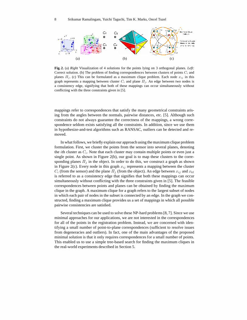
Fig. 2. (a) Right Visualization of 4 solutions for the points lying on 3 orthogonal planes.Left:Correct solution. (b) The problem of finding correspondences between clusters of pointsCi andplanesΠj . (c) This can be formulated as a maximum clique problem. Eachnodexij in thisgraph represents a mapping between clusterCi and planeΠj . An edge between two nodes isa consistency edge, signifying that both of these mappings can occur simultaneously withoutconflicting with the three constraints given in [5].

mappings refer to correspondences that satisfy the many geometrical constraints aris-ing from the angles between the normals, pairwise distances, etc. [5]. Although suchconstraints do not always guarantee the correctness of the mappings, a wrong corre-spondence seldom exists satisfying all the constraints. Inaddition, since we use themin hypothesize-and-test algorithms such as RANSAC, outliers can be detected and re-moved.

In what follows, we briefly explain our approach using the maximum clique problemformulation. First, we cluster the points from the sensor into several planes, denotingthe ith cluster asCi. Note that each cluster may contain multiple points or even just asingle point. As shown in Figure 2(b), our goal is to map theseclusters to the corre-sponding planesΠj in the object. In order to do this, we construct a graph as shownin Figure 2(c). Every node in this graphxij represents a mapping between the clusterCi (from the sensor) and the planeΠj (from the object). An edge betweenxij andxkl

is referred to as a consistency edge that signifies that both these mappings can occursimultaneously without conflicting with the three constraints given in [5]. The feasiblecorrespondences between points and planes can be obtained by finding the maximumclique in the graph. A maximum clique for a graph refers to thelargest subset of nodesin which each pair of nodes in the subset is connected by an edge. In the graph we con-structed, finding a maximum clique provides us a set of mappings in which all possiblepairwise consistencies are satisfied.

Several techniques can be used to solve these NP-hard problems [8, 7]. Since we useminimal approaches for our applications, we are not interested in the correspondencesfor all of the points in the registration problem. Instead, we are concerned with iden-tifying a small number of point-to-plane correspondences (sufficient to resolve issuesfrom degeneracies and outliers). In fact, one of the main advantages of the proposedminimal solution is that it only requires correspondences for a small number of points.This enabled us to use a simple tree-based search for finding the maximum cliques inthe real-world experiments described in Section 5.

P2Π: A Minimal Solution for Registration of 3D Points to 3D Planes 9

Fig. 3. A general framework to transform a given registration problem to a point-to-plane prob-lem. Left: In the sensor data, we transform all geometrical entities (points, lines and planes) topoints. A point is preserved as a point. In the case of lines and planes we sample two and threearbitrary points, respectively.Right: In the object data, we convert all geometrical entities toplanes. A plane is preserved as a plane. Points and lines are parameterized using 3-plane and2-plane representations, as shown.

4 A General Framework for Pose Estimation

We briefly sketch a unified pose estimation framework for most2D-to-3D and 3D-to-3D registrations by first transforming the given problem to apoint-to-plane registrationproblem. Several 2D-to-3D pose estimation algorithms havebeen proposed in the lit-erature [6, 18, 10, 1, 21, 5, 4, 20]. All of these pose estimation algorithms involve theregistration of one set of geometrical entities (points, lines, or planes) to another. Forexample, in the case of generalized pose estimation, we register three 3D points to thecorresponding non-parametric projection rays from the cameras to compute the poseof the object with respect to the camera [20]. In the case of 2D-to-3D pose estimationusing three lines, we can look at this problem as a registration of three interpretationplanes (each formed by two projection rays corresponding toa single line) on threelines [18]. In the case of 3D-to-3D line-to-plane registration, we register lines from thesensor data to planes from the object [4]. In the case of 3D-to-3D point-to-point regis-tration, we register points from sensor data to points in theobject [6]. One could alsopropose registration algorithm involving mixture of geometrical entities and thereby wecould have more than 20 2D-to-3D and 3D-to-3D registration scenarios. We emphasisthat any of these pose estimation algorithms involving any combination of geometricalentities to any other combination could be transformed to a point-to-plane registrationalgorithm and solved using the following simple algorithm.

1. In the sensor data, we transform all the geometrical entities (points, lines andplanes) to points. This is done using 2-point and 3-point representation of linesand planes respectively as shown in Figure 3.

2. In the object data, we transform all the geometrical entities to planes. This is doneby 3-plane and 2-plane representations for points and lines, respectively. Note thatthe 3 planes passing through a point need not be orthogonal. Similarly, we use 2non-orthogonal planes to represent a line. The appropriatechoice of these planesplays a crucial role in obtaining an efficient pose estimation algorithm.

3. After these transformations, we can use our point-to-plane registration algorithm.

Details of the proposed generalized framework are given in the Supplementary Ma-terials with examples on several registration problems.

10 Srikumar Ramalingam, Yuichi Taguchi, Tim K. Marks, OncelTuzel

Fig. 4. Rotation and translation error for simulation data as a function of the level of noise inthe test set. The noise standard deviation is expressed as a percentage of the size of the object.The legends list the configurations in order of decreasing error. (a,b) Results from our algorithmfor all non-degenerate configurations shown in Table 1. Notethat minimal solutions using 6points provide lower errors than non-minimal solutions, and solutions for configurations withlarger number of planes have lower errors. (b–j) Our minimalsolutions compared to least squaremethods (using 12 and 20 points) for the same number of planesn: (c,d) n = 3, (e,f) n = 4,(g,h)n = 5, and (i,j)n = 6. Note that in the 3-plane case (b), least square methods completelyfail due to rank degeneracy.

5 Experimental Results

Simulations: We analyzed the performance of our minimal solutions in simulations bygenerating 32 random planes inside a cube of side length 100 units. We randomly sam-pled 320 points on these planes within the cube. A test set wascreated by transformingall 320 points using a ground-truth rotation and translation, then adding Gaussian noiseto each point.

We randomly selectedk points from the test set according to the point-to-plane con-figuration of the algorithm, then computed the rotation and translation using the pointsand the corresponding planes. The estimated transformation was then evaluated by us-

P2Π: A Minimal Solution for Registration of 3D Points to 3D Planes 11

(a) (b)

Fig. 5. Real-world experiment with a 6-degrees-of-freedom robotic arm. (a) 3D contact positiondata were collected for 100 points on the surface using a built-in contact detection function andbuilt-in encoders of the robotic arm. (b) Plane fitting of the3D points and the correspondences ofthe points to the planes in the CAD model using the method of Section 3.

ing it to transform the other320 − k points and computing the mean point-to-planedistance between the transformed points and their correct corresponding planes. Eachtrial consists of generating a test set, then repeating the selection ofk points and trans-formation estimation 100 times for this test set. Of the resulting 100 transformations,the solution for the trial is the one transformation that provides the minimum meandistance.

Figure 4 plots errors in estimated rotation and translationwith varying noise levels.For each configuration, the errors plotted are the average of100 trials. For each numberof planes (n = 3, 4, 5, 6), we compare our minimal solutions for every possible con-figuration of 6 points (as well as the non-minimal configurations for 3 planes that wereincluded in Table 1) to a least-squares solution for the samenumber of planes using12 or 20 points without orthonormality constraints. In all cases, our minimal solutionsyield smaller errors than the least squares method. Note that the least squares methodcompletely fails in the case of three planes. Thus, our transformation is useful not onlyfor the minimal configurations but also in non-minimal configurations such as(3, 3, 3).

Contact Sensor: The first experiment, shown in Figure 5, was conducted using a6-degree-of-freedom robotic arm with a built-in contact detection function. We used asthe target object a partial surface of an icosahedron, of which four of the 20 faces aremeasurable, as shown in Figure 5. The robot automatically measured 100 points (con-tact positions) on the surface; each point was measured by first moving the probe toa randomx, y position and then moving down towards the surface (in the negativez

direction) until it sensed a contact. We clustered the points using a simple RANSAC-based plane fitting algorithm. There were four main clusterscorresponding to the fourplanes of the icosahedron used in the experiment. Next, the method described in Sec-tion 3 was used to find the correspondences between these clusters and the planes in the3D model. Given these correspondences, we applied our point-to-plane algorithm usingseveral of the minimal 3-plane and 4-plane configurations. As in the simulations, werepeated the following process to determine the solution: randomly selectingk points,

12 Srikumar Ramalingam, Yuichi Taguchi, Tim K. Marks, OncelTuzel

(a) (b) (c)

Fig. 6. (a) An input stereo pair of photos taken in Boston’s financialdistrict, overlaid with thepoints that we matched and reconstructed in 3D. (b) We identify four clusters in the reconstructed3D points (a single point and three planar clouds of points) using a plane-fitting algorithm. (c)The four planes in the 3D city model corresponding to the identified clusters shown in (b).

solving for the transformation, and evaluating the mean distance of the transformed re-maining points to the 3D model. The final point-to-plane distance error for all of theinliers was about3% of the overall size of the scene. The least squares method failedcompletely for the 3-plane case (similar to the results shown in Figure 4). In the 4-planecase, the least-squares error was about 10 times larger thanthe error of the minimalsolutions.

Registration of 3D point clouds to polyhedral architectural models: Given a plane-approximated coarse 3D model of the city of Boston obtained from a commercial web-site (http://www.3dcadbrowser.com/), we performed localization within the map usinga pair of images of a scene in Boston’s financial district. To obtain 3D points fromthe image pair, we matched Harris features and applied standard structure-from-motionalgorithms.

Using a RANSAC-based plane fitting algorithm, we fit planes tothe reconstructed3D points. We computed 3 planes from the reconstructed points as shown in Figure 6.A coarse initialization is manually provided and the nearest planes in the 3D modelare identified. All of the planes shown in Figure 6(c) (more than 10 planes) were usedfrom the 3D model of Boston. Using the method described in Section 3, we obtained thecorrespondences between four clusters (a single point and three planar clouds of points)and four planes in the 3D model. The plane corresponding to the ground had only one3D point due to occlusion from pedestrians and cars. (Note that it was important to haveat least one point on the ground in order to determine the vertical translation.) Applyingour minimal algorithms for the 4-planes case yielded results with an error of just0.05%of the overall size of the scene.

Our point-to-plane registration algorithm can also be usedfor merging partial re-constructions obtained from multi-view reconstruction techniques [22, 23], as shownin Figure 7. In order to obtain a 3D model from 30 images, we subdivide the imagesinto two clusters of 15 images each. We reconstruct 3D point clouds from each im-age cluster and use the superpixel segmentation of a common image to register them.The 3D points from the first cluster are reprojected onto the superpixel image and usedto compute the plane parameters for each superpixel. (We eliminate superpixels with

P2Π: A Minimal Solution for Registration of 3D Points to 3D Planes 13

(a) (b) (c) (d)

Fig. 7.Registering two point clouds, each generated by applying multi-view reconstruction tech-niques to 15 images.(a) One of the images used in 3D reconstruction.(b) superpixel segmenta-tion of the image shown in (a).(c) The 3D points from the first (blue) and second (red) cloudsare reprojected onto the superpixel image. The points from the first point cloud are used to com-pute the superpixel plane parameters, while the second point cloud is preserved as points. Thecorrespondence between the points from the second cloud andthe planes obtained from the firstcloud are determined by the underlying superpixel.(d) 3D model after merging the two partialreconstructions from the two clusters. [Best viewed in color]

insufficient or non-planar points.) The superpixel segmentation of the common imagegives us the correspondences between the points in the second cluster and the planesobtained from the first cluster. We obtain the 3D registration using a RANSAC frame-work, in which we select three or more non-degenerate planes(See section 2.4) and thecorresponding minimum number of points.

Previous work merging partial 3D models obtained multi-view 3D reconstructionhas used non-minimal iterative approaches [24]. However, initializing with a minimalsolution, such as the one described here, may be critical fornoisy 3D data. In addition,there are two general advantages of point-to-plane rather than point-to-point registra-tion: (1) accuracy [25], (2) compact representation of the 3D models (about a million3D points are represented using few hundred superpixel planes).

6 Discussion

The development of minimal algorithms for registering 3D points to 3D planes providesopportunities for efficient and robust algorithms with wideapplicability in computervision and robotics. Since 3D sensors typically do not perceive the boundaries of objectsin the same way as 2D sensors, an algorithm that can work with points on the surfaces,rather than surface boundaries, is essential. In textureless 3D models, for example, itis easier to obtain point-to-plane correspondences than point-to-point and line-to-linecorrespondences.

Acknowledgments:We would like to thank Jay Thornton, Keisuke Kojima, John Barn-well, and Haruhisa Okuda for their valuable feedback, help and support.

14 Srikumar Ramalingam, Yuichi Taguchi, Tim K. Marks, OncelTuzel

References

1. Olsson, C., Kahl, F., Oskarsson, M.: The registration problem revisited: Optimal solutionsfrom points, lines and planes. In: CVPR. Volume 1. (2006) 1206–1213

2. Besl, P., McKay, N.: A method for registration of 3D shapes. In: PAMI. (1992)3. Fitzgibbon, A.: Robust registration of 2d and 3d point sets. In Image and Vision Computing

(2003)4. Chen, H.: Pose determination from line-to-plane correspondences: Existence condition and

closed-form solutions. PAMI13 (1991) 530–5415. Grimson, W., Lozano-Prez, T.: Model-based recognition and localization from sparse range

or tactile data. MIT AI Lab, A.I. Memo 738 (1983)6. Horn, B.: Closed-form solution of absolute orientation using unit quaternions. Journal of the

Optical Society A4 (1987) 629–6427. Li, H., Hartley, R.: The 3D-3D registration problem revisited. In: ICCV. (2007) 1–88. Enqvist, O., Josephson, K., Kahl, F.: Optimal correspondences from pairwise constraints.

In: ICCV. (2009)9. Tu, P., Saxena, T., Hartley, R.: Recognizing objects using color-annotated adjacency graphs.

In: In Lecture Notes in Computer Science: Shape, Contour andGrouping in Computer Vi-sion. (1999)

10. Chen, Y., Medioni, G.: Object modeling by registration of multiple range images. In: ICRA.Volume 3. (1991) 2724–2729

11. Kukelova, Z., Pajdla, T.: A minimal solution to the autocalibration of radial distortion. In:CVPR. (2007)

12. Gao, X., Hou, X., Tang, J., Cheng, H.: Complete solution classification for the perspective-three-point problem. PAMI25 (2003) 930–943

13. Stewenius, H., Nister, D., Kahl, F., Schaffalitzky, F.:A minimal solution for relative posewith unknown focal length. In: CVPR. (2005)

14. Stewenius, H., Nister, D., Oskarsson, M., Astrom, K.: Solutions to minimal generalizedrelative pose problems. In: OMNIVIS. (2005)

15. Geyer, C., Stewenius, H.: A nine-point algorithm for estimating para-catadioptric fundamen-tal matrices. In: CVPR. (2007)

16. Li, H., Hartley, R.: A non-iterative method for correcting lens distortion from nine-pointcorrespondenses. In: OMNIVIS. (2005)

17. Fischler, M., Bolles, R.: Random sample consensus: A paradigm for model fitting withapplications to image analysis and automated cartography.Communications of the ACM24(1981) 381–395

18. Dhome, M., Richetin, M., Lapreste, J.T., Rives, G.: Determination of the attitude of 3-Dobjects from a single perspective view. PAMI11 (1989) 1265–1278

19. Kukelova, Z., Bujnak, M., Pajdla, T.: Automatic generator of minimal problem solvers. In:ECCV. (2008)

20. Nister, D.: A minimal solution to the generalized 3-point pose problem. In: CVPR. (2004)21. Haralick, R., Lee, C., Ottenberg, K., Nolle, M.: Review and analysis of solutions of the three

point perspective pose estimation problem. IJCV (1994)22. Furukawa, Y., Ponce, J.: Accurate, dense, and robust multi-view stereopsis. PAMI (2009)23. Furukawa, Y., Ponce, J.: Patch-based multi-view stereosoftware (200)

http://grail.cs.washington.edu/software/pmvs.24. Ramalingam, S., Lodha, S.: Adaptive enhancement of 3d scenes using hierarchical registra-

tion of texture-mapped 3d models. In: 3DIM. (2003)25. Rusinkiewicz, S., Levoy, M.: Efficient variants of the icp algorithm. In: 3DIM. (2001)