P8A.16 L-Moment Method Applied to Observed Raindrop Size Distributions

Donna V. Kliche, Andrew G. Detwiler, Paul L. Smith, and Roger W. Johnson South Dakota School of Mines and Technology, Rapid City, SD, USA

Abstract The parameter-fitting method of L-moments is applied to measurements of raindrop sizes collected with the two-dimensional cloud probe (2D-C) instrument on the T-28 research aircraft. We consider expo-nential, gamma, and lognormal approximations of the observed size distributions. The results for the fitted parameters obtained from these observations are compared with results from the alternative methods of moments or maximum likelihood, and with computer-simulated results. 1. Introduction

To describe analytically a raindrop spectrum collected, one has to assume first a certain mathematical distribution that could be appropriate to describe the raindrop population from which the sample was taken. The raindrop size distribution (RSD) is expressed in terms of a distribution func-tion n(D), which represents the number of drops per unit size interval per unit volume of space.

The most used description for the raindrop spectrum in space is the size distribution of Mar-shall and Palmer (1948), which is of exponential form and has two parameters:

)exp()( 0 ΛDnDn −= , ( 0≥D ) (1)

where D is the drop diameter, n0 is the value of n(D) for D = 0 and Λ is the scale (size) parameter. In a semi-logarithmic plot, equation (1) becomes the graph of a straight line with Λ as slope and n0 as the y-intercept. However, the exponential dis-tribution is not able to describe the variety of the observed spectra (Waldvogel and Joss, 1970; Waldvogel, 1974; Joss and Gori, 1978; Ulbrich, 1983; Steiner and Waldvogel, 1987; Tokay et al., 2002; Lee and Zawadzki, 2005). Use of the gamma distribution (Ulbrich, 1983; Willis, 1984), which seemed to give a more appropriate descrip-tion of the natural variations of the observed RSDs, was therefore proposed (the exponential distribution is a special case). A gamma RSD can be expressed by

)exp()( 1 DDnDn λμ −= , ( 0≥D ) (2)

where n1 is related to the raindrop concentration, µ is the dimensionless shape parameter of the distribution, and λ is the scale parameter. The gamma distribution is widely accepted by the radar meteorology and cloud physics communities (e.g. Wong and Chidambaram, 1985; Chandrasekar and Bringi, 1987; Kozu and Nakamura, 1991; Haddad et al., 1996; Tokay and Short, 1996; Ul-brich and Atlas, 1998; Zhang et al., 2003), al-though measurements of RSDs show that even the gamma distribution is not general enough to represent adequately the full range of observed RSDs.

Feingold and Levin (1986) used another func-tion to represent RSD, i.e., the three-parameter lognormal distribution. The lognormal distribution is related to the normal distribution through the fact that it involves a logarithmic transformation of the data, with the assumption that the resulting transformed data are described by a normal distri-bution (Wilks, 1995; Cerro et al., 1997). In terms of raindrop diameters, the lognormal distribution can be written as

⎪⎭

⎪⎬⎫

⎪⎩

⎪⎨⎧

⎥⎦

⎤⎢⎣

⎡−=

2

ln)/ln(

21exp

2ln)(

σπσgT DD

DNDn ,( 0≥D )(3)

where NT is the total number concentration; Dg is the scale parameter, which represents the geo-metric mean of the raindrop diameters (or median diameter) and is defined by ( ) ( )[ ]DEDg lnln = . (4)

The dimensionless shape parameter, σln , is the standard deviation of the natural log of the rain-drop diameters (standard geometric deviation) and is defined by

Corresponding author address: Dr. Donna V. Kliche, SDSM&T, 501 East Saint Joseph St., Rapid City, SD 57701-3995; E-mail: donna.kliche@sdsmt.edu

( )[ ]2lnlnln gDDE −=σ . (5)

Typically, in statistical literature the notation for the lognormal shape parameter is σ rather than σln , but the meaning is the same with (5).

Regardless of the function chosen to repre-sent the RSD, some means of determining the parameters appropriate for any given set of obser-vations is needed. Apart from fitting by eye, as in Marshall and Palmer (1948), possibilities include the method of moments, the method of maximum likelihood (ML), and the L-moment method. These three methods and the corresponding equations in the case of the gamma distribution are discussed in detail in Kliche et al. (2007a).

2. Data

During T-28 Flight 817 (28 July 2003), the precipitation particles were imaged with a PMS optical array probe (2D-C). This probe produces shadow images of precipitation-size particles with a vertical window height of 0.8 mm and a pixel resolution of 0.025 mm. A brief discussion of the T-28 probe is given in Detwiler and Hartman (1991). One important limitation of this probe is its poor sampling capability in the diameters range < 0.2 mm (due to optical and resolution problems) as well as in the larger sizes due to the small vol-ume sampling capability (0.05 m3/km). This probe performed well during this flight, and an example of the recorded data is shown in Figure 1.

This research flight originated in Greeley, in

the northeast corner of the state of Colorado, USA, in the western High Plains of North America. The terrain is rolling short grass prairie. The target of the flight was a disorganized group of thunder-storms with echo tops reaching 12 km MSL. The aircraft conducted a series of passes through rain shafts at an altitude of 3 km MSL, roughly 1.5 km AGL and just below cloud base. Cloud base tem-perature was 10 0C and the temperature at flight level was about 12 0C. Polarimetric radar showed peak echo magnitudes of 50 dBZ, and Zdr ranging from zero to one dB, at altitudes above the 0 0C level. A distinct bright band was visible at 4.7 km

MSL (3.2 km AGL) in the stratiform regions down-shear of the convective cores. These observations are consistent with precipitation formation in the convective region producing the rainshafts by the growth of graupel through the riming of ice crystals and crystal aggregates, with melting to rain below cloud.

We selected one minute of the data collected,

from 21:44:29 to 21:45:31 UTC. We considered samples each taken during 5 seconds of flight, i.e. about 500 meters traveled by the T-28 aircraft. A total of 13 samples were acquired from the data collected during the one minute interval. We se-lected only particles that were equal to or greater than 3 pixels in size (i.e., 0.075 mm or larger); we refer to the samples as being “censored.” The di-ameters for particles that were only partially im-aged by the probe were determined based on an algorithm described in Detwiler and Hartman (1991). The effective sample volume varies with the particle diameter, but the data have not yet been adjusted to account for that fact. Table 1 shows the number of drops collected, and the minimum and maximum drop diameter, for each sample. The sample sizes correspond (with only one exception) to the medium sample size classi-fication (20 ≤ NT < 100), based on the classifica-tion described in Kliche et al. (2006).

3. Method of Analysis

The process has to begin with assuming some

form for the drop size distribution function, say, exponential, gamma or logarithmic. For example, given a measured sample of drops, one may as-sume that an exponential distribution should de-scribe analytically the raindrop spectrum. The next step is to estimate the parameters for the as-sumed distribution using the sample data.

The traditional approach with experimental

RSD data has been to use the method of mo-ments to estimate the parameters for the RSDs. The moments calculated from the sample data can be used to estimate the parameters of the as-sumed underlying exponential (or gamma or log-normal) distributions. In Kliche et al. (2007a) the three-moment combinations M2M3M4, M2M4M6 and

Figure 1: Example of the 2D-C recorded data during T-28 Flight 817 (28 July 2003). The duration for this buffer was 1.003 s and the distance traveled by the airplane during this time is about 100 m.

Buffer image: from 21:45:17.996 to 21:45:18.999 Duration: 1.003 s Distance: 100 m

M3M4M6, where Mi represents the ith moment of the distribution, are discussed in detail, and the corresponding equations for the gamma estima-tors are also given. The exponential case is pre-sented in detail in Smith and Kliche (2005) and Smith et al. (2005).

However, the moment method is known to be

biased (Robertson and Fryer, 1970; Wallis, 1974; Haddad et al., 1996, 1997; Smith and Kliche, 2005; Uijlenhoet et al., 2006), which means that the fitted functions often do not correctly represent the raindrop populations, and sometimes not even the samples. Smith and Kliche (2005), Smith et al. (2005), Kliche et al. (2006) and Kliche et al. (2007a) describe that the skewness in the sam-pling distributions of the RSD moments is the main cause for this bias. The bias is stronger when higher-order moments are considered in calculat-ing the parameters of the “fitted” functions, and the combination of 2nd, 3rd

, and 4th moments typically gives the smallest bias for three-parameter distri-butions. (Although lower-order moments would be desirable in such estimations, they can be poorly determined because of instrumental deficiencies.)

A second approach with experimental RSD

data would be to use the maximum likelihood (ML) method to estimate the parameters for the RSDs. For the exponential distribution the ML method is equivalent to the moment method (if the zeroth and first moments are used); in the case of the gamma or lognormal distribution, the calculation of the maximum likelihood estimators requires more effort. The steps to be followed in using this method and the corresponding equations for the

gamma distribution are given in Kliche et al. (2007a).

A third approach with the data would be to use

the L-moment method (Hosking and Wallis, 1997), which has been used for the first time for RSDs by Kliche et al. (2006). The L-moment approach is typically superior to ML with small samples. The corresponding equations for the gamma RSD case are given in Kliche et al. (2007a). In the case of the exponential distribution the moment (with M0 and M1), ML and L-moment methods are identical (Hosking and Wallis, 1997).

We applied each of these methods for the 13

samples listed in Table 1. We assumed that the samples come from drop populations that can be described by an exponential, gamma or lognormal RSD.

4. Results for Assumed Exponential Distributions

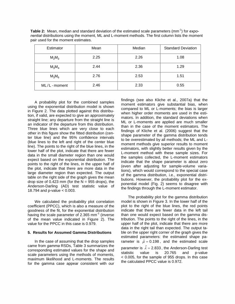
Table 2 gives the mean, median, and standard deviation values for the 13 scale parameter esti-mates using the moment, ML and L-moment methods, in the case of assuming that the drop samples came from exponential RSD. Comparing the values obtained for the scale parameter, it is obvious that higher order moments give larger es-timates; according to Smith and Kliche (2005), the best moment estimators are ones derived using the lower order moments. In the case of ML or L-moment estimators, the expectation is to get re-sults with essentially no bias for samples of these sizes (Kliche et al., 2006). Those estimators also yield the smallest standard deviation.

Table 1: Summary of the T-28 Raindrop Samples

Sample

#

Number of drops

Minimum Diameter

[mm]

Maximum Diameter

[mm]

Sample

#

Number of drops

Minimum Diameter

[mm]

Maximum Diameter

[mm] 1 44 0.075 2.875 8 87 0.075 2.550

2 78 0.075 3.756 9 67 0.075 1.750

3 32 0.075 0.900 10 81 0.075 3.381

4 100 0.075 2.350 11 80 0.075 2.800

5 107 0.075 2.075 12 95 0.075 2.375

6 67 0.075 1.156 13 18 0.075 4.450

7 99 0.075 4.100

A probability plot for the combined samples using the exponential distribution model is shown in Figure 2. The data plotted against this distribu-tion, if valid, are expected to give an approximately straight line; any departure from the straight line is an indicator of the departure from this distribution. Three blue lines which are very close to each other in this figure show the fitted distribution (cen-ter blue line) and the 95% confidence intervals (blue lines to the left and right of the center blue line). The points to the right of the blue lines, in the lower half of the plot, indicate that there are fewer data in the small diameter region than one would expect based on the exponential distribution. The points to the right of the lines, in the upper half of the plot, indicate that there are more data in the large diameter region than expected. The output table on the right side of the graph gives the mean drop size of 0.423 mm (for the N = 955 drops), the Anderson-Darling (AD) test statistic value of 18.794 and p-value < 0.003.

We calculated the probability plot correlation

coefficient (PPCC), which is also a measure of the goodness of the fit, for the exponential distribution having the scale parameter of 2.365 mm-1 (inverse of the mean value indicated in Figure 2). The value for the PPCC in this case is 0.979.

5. Results for Assumed Gamma Distributions

In the case of assuming that the drop samples

came from gamma RSDs, Table 3 summarizes the corresponding estimated values for the shape and scale parameters using the methods of moments, maximum likelihood and L-moments. The results for the gamma case appear consistent with our

findings (see also Kliche et al., 2007a) that the moment estimators give substantial bias, when compared to ML or L-moments; the bias is larger when higher order moments are used in the esti-mators. In addition, the standard deviations when ML or L-moments are applied are much smaller than in the case of the moment estimators. The findings of Kliche et al. (2006) suggest that the shape parameter of the gamma distribution tends to be overestimated by all methods; the ML and L-moment methods give superior results to moment estimators, with slightly better results given by the L-moment method with these sample sizes. For the samples collected, the L-moment estimators indicate that the shape parameter is about zero (even after adjusting for sample-volume varia-tions), which would correspond to the special case of the gamma distribution, i.e., exponential distri-butions. However, the probability plot for the ex-ponential model (Fig. 2) seems to disagree with the findings through the L-moment estimator.

The probability plot for the gamma distribution

model is shown in Figure 3. In the lower half of the plot to the right of the blue lines, the red points indicate that there are fewer data in the left tail than one would expect based on the gamma dis-tribution. The points to the right of the lines, in the upper half of the plot, indicate that there are more data in the right tail than expected. The output ta-ble on the upper right corner of the graph gives the estimated parameters: the estimated shape pa-rameter is 198.0ˆ =μ , and the estimated scale

parameter is 833.2ˆ =λ , the Anderson-Darling test statistic value is 20.765 and p-value < 0.005, for the sample of 955 drops. In this case the calculated PPCC value is 0.972.

Table 2: Mean, median and standard deviation of the estimated scale parameters (mm-1) for expo-nential distributions using the moment, ML and L-moment methods. The first column lists the moment pair used for the moment estimates.

Estimator Mean Median Standard Deviation

32MM 2.25 2.26 1.08

43MM 2.44 2.36 1.29

63MM 2.76 2.53 1.51

moment-L/ML 2.46 2.33 0.55

Figure 2: Probability plot of the data (red) against an assumed exponential distribution. The three blue lines represent the fitted distribution (centered blue line) and the confidence interval lines (to the right and left of the centered line). Population RSD: assumed to be exponential. The “D-censored” refers to the sample having drop diameter D ≥ 0.075 mm.

Table 3: Mean, median and standard deviation of the estimated shape ( )μ̂ and, in parentheses, scale

( )λ̂ parameters for the gamma distributions using the moment, ML and L-moment methods.

Estimator Mean Median Standard Deviation

432 MMM 2.12 (3.97) 1.21 (2.75) 2.95 (3.90)

642 MMM 6.80 (6.71) 3.89 (4.50) 9.53 (7.40)

643 MMM 18.94 (10.72) 6.02 (5.37) 42.10 (13.27)

ML 0.27 (3.22) 0.23 (2.87) 0.25 (1.22)

momentL − -0.01 (2.51) -0.01 (2.19) 0.27 (1.08)

With the data shown in the probability plots for exponential and gamma approximations, one could conclude that the measured raindrop sample probably cannot be approximated by either expo-nential or gamma distributions. However, the fit shown in Figure 2 seems to be superior to the one shown in Figure 3. The left tail in Figure 2 is caused by a lack of sufficient small drops in the data, but it is also due to the truncation imposed by us for the smaller drop diameters (D ≥ 0.075), and by the pixel quantification of the drop sizes.

6. Results for Assumed Lognormal Distributions

Similarly, we assumed that the population from which the samples were taken could be de-scribed by the lognormal function (3). Table 4 gives the mean, median, and standard deviation values for the shape and scale estimators using the methods of moments, maximum likelihood and L-moments. In the case of the lognormal distribu-tion (Kliche, 2007), the ML and L-moment meth-ods should give results without significant bias.

Figure 3: Probability plot of the data (red) against an assumed gamma distribution. The three blue lines represent the fitted distribution (centered blue line) and the confidence interval lines (to the right and left of the centered line). The shape parameter estimate given in the box is ( μ̂1+ ), and

the scale parameter estimate is λ̂1 . Population RSD: assumed to be gamma. The “D-censored” refers to the sample having drop diameter D ≥ 0.075 mm.

Table 4: Mean, median and standard deviation of the estimated shape ( )σ̂ln and, in parentheses,

scale ( )gD̂ parameters for the lognormal distribution using the moment, ML and L-moment methods.

Estimator Mean Median Standard Deviation

432 MMM 0.45 (1.02) 0.46 (0.75) 0.09 (0.75)

642 MMM 0.34 (1.34) 0.35 (1.01) 0.08 (0.89)

643 MMM 0.29 (1.56) 0.30 (1.10) 0.08 (0.99) ML 0.93 (0.27) 0.90 (0.27) 0.09 (0.05)

momentL − 0.98 (0.26) 0.96 (0.26) 0.12 (0.05)

The mean value for the shape parameter from the ML and L-moment methods in Table 4 is about 0.9-1.0, which represents a wide lognormal distri-bution with a very long tail to the right. This means that the distribution function (3) would have to be truncated at some realistic maximum diameter, and the estimators recalculated accordingly. The widest lognormal distribution discussed by Kliche (2007) had a shape parameter of 0.5; therefore, for the purpose of this work, only the gamma dis-tribution form was studied in further detail.

7. Results for Individual Samples

For each 5 s sample we consider here, the

gamma RSD parameters were calculated using the two moment combinations, M2M3M4, and M3M4M6, as well as the ML and L-moment estima-tors. Figure 4 shows a comparison of cumulative histograms of the estimates of the scale parameter λ for a gamma RSD. This and the next figure demonstrate how the increase of the sampling skewness with the moment order translates into greater biases for the estimated parameters when higher-order moments are used. The M2M3M4 combination seems to agree well with the ML or L-moment estimators, except for two samples.

The corresponding cumulative histograms for the estimated gamma shape parameter ( μ̂ ) are given in Figure 5. This figure demonstrates again that larger bias is given by using higher order mo-ments. Based on our findings (Kliche, 2007), both the ML and L-moment estimators should be the closest to the true population value; they suggest a value not far different from zero (i.e., an expo-nential RSD) for each individual sample.

8. Results for Composite Sample

Figure 6 gives the composite histogram of all

the drops from the samples collected during the one minute flight segment (955 drops). Overlaid distributions correspond to the estimated RSD pa-rameters using the L-moment, ML and moment methods. The continuous red line corresponds to the M3M4M6 case, the continuous green line, dot-ted red line and dash-dot red line (which all coin-cide) correspond to ML, M2M3M4 and M2M4M6 re-spectively. The blue line corresponds to the L-moments case. Even though the curves differ, it appears from this figure, that all the estimators give comparable results over the range of sizes included in the analysis. This is not a surprise, since the composite sample (from adding all 13 samples collected during one minute of T-28 flight) consisted of 955 drops. Based on the results de-scribed in Kliche et al. (2007a), when large enough samples are available the three fitting

Figure 4: Cumulative histograms of estimated gamma scale parameter, λ̂ , using the M2M3M4 set (black), M3M4M6 set (red), ML (green) and L-moments (blue). Population RSD: assumed to be gamma.

Figure 5: Cumulative histograms of estimated gamma shape parameter, μ̂ , using the M2M3M4 set (black), M3M4M6 set (red), ML (green) and L-moments (blue). Population RSD: assumed to be gamma.

methods are expected to give comparable results. A suitable goodness-of-fit test would be needed to discriminate among these estimators.

9. Correlation Issues

The correlations between the sample mo-

ments and the maximum drop diameter Dmax in the sample were the first correlations investigated. Figure 7 shows an example of such correlation, for the case of the 6th moment (proportional to reflec-tivity factor); these are individual samples, not necessarily from the same population, but a simi-lar correlation with nearly identical correlation co-efficient showed up in the simulations of repetitive sampling from an exponential RSD with mean sample size 100 drops (Kliche, 2007).

The sample moments are also correlated with

each other; Figure 8 shows such a correlation be-tween the 3rd and 6th sample moments. The slope of this relationship would correspond to an exponent 2.44 in the “Z-W” relationship, but this “relationship” may be due here only to the variabil-

ity in the samples taken from a common raindrop population.

The correlations of the various sample mo-

ments with the maximum drop size in a sample, and the associated correlations between mo-ments, lead to correlation of the “fitted” gamma parameters with the maximum drop size. Figure 9 shows the correlation between the mass-weighted

Figure 6: Histogram corresponding to the T-28 data collected during 21:44:29 to 21:45:31 UTC (955 drops); curves using the gamma PDF function (Kliche et al., 2007a) from the parame-ters using the L-moment ( )01.0ˆ −=LMμ , ML ( )27.0ˆ =MLμ and moment (shape parame-ter: M2M3M4 = 2.12; M2M4M6 = 6.8; M3M4M6 = 18.94) fitting methods.

Figure 7: Scatter plot of 6th sample moment values versus the maximum drop diameter in the sample; the correlation coefficient is 0.971.

Figure 8: Scatter plot of 3rd versus 6th sam-ple moment values; the correlation coefficient is 0.972.

mean diameter estimates ( )mD̂ and the maximum drop diameter in the samples. This figure provides a comparison between the estimated values using the moments M3M4M6 with ones from the ML and L-moment estimators.

A second example of such correlations is

shown in Figure 10 for the normalized concentra-tion parameter WN̂ (defined in Bringi and Chandrasekar, 2001) and the maximum drop size in the sample. The correlations in the case of the ML and L-moment estimators are weaker than in the case of the moment estimators.

Correlations also exist between the estimated

parameters; results from simulations of repetitive sampling (Kliche, 2007) suggest that one should be very cautious in inferring any physical relation-ships between such “fitted” parameters. Figure 11 gives examples of such correlations between the mass-weighted mean diameter ( )mD̂ versus total

number concentration ( )TN̂ , in the case of M2M3M4

and M3M4M6 estimators as compared to the ML and L-moment estimators. The ML and L-moment estimators are correlated, but their correlation is weaker than in the case of the moment estimators, and is not significant under an assumption of nor-mally-distributed residuals.

Figure 9: Scatter plot of estimated mass-weighted mean diameter ( )mD̂ versus the maximum diame-ter in the samples: M3M4M6 (black, r = 0.959), ML (red, r = 0.763), L-moments (green, r = 0.799).

Figure 10: Scatter plot of the estimated nor-malized concentration parameter ( )WN̂ ver-sus the maximum diameter in the samples: M3M4M6 (black, r = -0.878), ML (red, r = -0.578), LM (green, r = -0.606). Popula-tion RSD: assumed to be gamma.

Figure 11: Scatter plot of the estimated total number concentration parameter ( )TN̂ versus

the mass-weighted mean diameter ( )mD̂ : M2M3M4 (black, r = -0.527), M3M4M6 (red, r = -0.780) ML (green, r = -0.231), L-moments (blue, r = -0.351). Population RSD: assumed to be gamma.

Special attention needs to be given to experi-mental data when such correlations are investi-gated. In many occasions one or two points in the scatter plot can affect this correlation dramatically. We show such an example for the case of the M3M4M6 estimators, λ̂ vs. μ̂ , in Figure 12. The correlation coefficient in this case is calculated to be 0.705. However, a careful look into this graph shows two experimental points well separated from the main cluster; these points correspond to the “outlier” cases in Figures 4 and 5. Figure 13 shows the same graph as in Figure 12, with the two outlying points removed. Now the correlation is not significant.

For the L-moment and ML estimators, the λ̂ vs. μ̂ correlation still exists and there is no indica-tion of outlier points. Figure 14 gives the corre-sponding scatter plot for these estimators, show-ing a correlation of about 0.9. Simulation results in Kliche (2007) show similar correlation coefficients for the ML and L-moment, λ̂ vs. μ̂ estimators, arising from repetitive sampling from the same population.

Figure 12: Scatter plot of the estimated M3M4M6 scale parameter λ̂ vs. M3M4M6

shape parameter μ̂ ; the correlation coeffi-cient is r=0.705. Population RSD: assumed to be gamma. All 13 samples considered.

Figure 13: Scatter plot of the estimated M3M4M6 scale parameter λ̂ vs. μ̂ shape parameter. Correlation coefficient is 0.284. Only 11 samples considered.

Figure 14: Scatter plot of the estimated scale parameter λ̂ vs. shape parameter μ̂ : ML (r = 0.899) in black; L-moments (r = 0.902) in red. Population RSD: assumed to be gamma. All 13 samples are considered.

10. Conclusions The main goal for the present work was to ap-

ply the L-moments method described in Kliche et al. (2007a) to real raindrop data collected during T-28 Flight 817, and to compare the results with findings from those simulations. The L-moments method was applied, and the results were com-pared to the ones obtained with the moment method and the maximum likelihood method.

As shown in Kliche et al. (2007a), the L-

moment parameters for gamma distributions have the smallest bias of the three fitting methods stud-ied (moments, ML, L-moments). The results for the real data used in this study appear to be con-sistent with those simulation results. The least bi-ased estimators suggest that these raindrop size distributions, observed just below cloud base at about 12 0C, are approximately exponential.

Acknowledgement: This research work was

partially supported by NSF Grant ATM-0531690.

11. References Bringi, V.N., and V. Chandrasekar, 2001: Po-

larimetric Doppler Weather Radar: Principles and Applications, Cambridge University Press, 636p.

Cerro, C., B. Codina, J. Bech, and J. Lorente, 1997: Modeling raindrop size distributions and Z(R) relations in the Western Mediterranean area. J. Appl. Meteor., 36, 1470-1479.

Chandrasekar, V., and V.V. Bringi, 1987: Simula-tion of radar reflectivity and surface measure-ments of rainfall. J. Atmos. Oceanic Technol., 4, 464-478.

Detwiler, A.G. and K.R. Hartman, 1991: IAS method for 2D data analysis on PCs. Bulletin 91-5, Institute of Atmospheric Sciences, SDSM&T, 37 pp. + appendices.

Feingold, G., and Z. Levin, 1986: The lognormal fit to raindrop spectra from frontal convective clouds in Israel. J. Climate Appl. Meteor., 25, 1346-1363.

Haddad, Z.S., S.L. Durden, and E. Im, 1996: Pa-rameterizing the raindrop size distribution. J. Appl. Meteor., 35, 3-13.

Haddad, Z.S., D.A. Short, S.L. Durden, E. Im, S. Hensley, M.B. Grable, and R.A. Black, 1997: A new parameterization of the rain drop size dis-tribution. IEEE Transactions of Geosciences and Remote Sensing, 35, 532-539.

Hosking, J.R.M. and J.R. Wallis, 1997: Regional Frequency Analysis: An Approach Based on L-Moments, Cambridge University Press.

Joss, J. and E. G. Gori, 1978: Shapes of raindrop size distributions. J. Appl. Meteor., 17, 1054-1061.

Kliche, D.V., 2007: Raindrop Size Distribution Functions: An Empirical Approach. PhD. Dis-sertation, SDSM&T, 211 pgs.

Kliche, D.V., P.L. Smith and R. W. Johnson, 2006: Estimators for parameters of drop-size distri-bution functions: sampling from gamma distri-butions, 12th Conference on Cloud Physics, Madison, WI, Amer. Meteor. Soc.

Kliche, D.V., P.L. Smith, R.W. Johnson, 2007a: L-Moment estimators as applied to exponen-tial, gamma, and lognormal drop size distribu-tions. 33rd Conf. on Radar Meteorology, Cairns, Australia, Amer. Meteor. Soc.

Kliche, D.V., A.G. Detwiler, P.L. Smith, and R.W. Johnson, 2007b: L-Moment method applied to observed raindrop size distribution. 33rd Conf. on Radar Meteorology, Cairns, Australia, Amer. Meteor. Soc.

Kliche, D.V., A.G. Detwiler, P.L. Smith, and R.W. Johnson, 2007b: L-Moment method applied to observed raindrop size distribution. 33rd Conf. on Radar Meteorology, Cairns, Australia, Amer. Meteor. Soc.

Kozu, T., and K. Nakamura, 1991: Rainfall pa-rameter estimation from dual-radar measure-ments combining reflectivity profile and path-integrated attenuation. J. Atmos. Oceanic Technol., 8, 259-270.

Lee, G., and I. Zawadzki, 2005: Variability of drop size distributions: time-scale dependence of the variability and its effects on rain estima-tion. J. Appl. Meteor., 44, 241-255.

Marshall, J. S. and W. McK. Palmer, 1948: The distribution of raindrops with size. J. Meteor., 5, 165-166.

Robertson, C.A., and J.G. Fryer, 1970: The bias and accuracy of moment estimators. Bio-metrika, 57, 57-65.

Smith, P. L. and D. V. Kliche, 2005: The bias in moment estimators for parameters of drop-size distribution functions: sampling from ex-ponential distributions. J. Appl. Meteor., 44, 1195-1205.

Smith, P. L., D. V. Kliche and R. W. Johnson, 2005: The bias in moment estimators for pa-rameters of drop-size distribution functions: sampling from gamma distributions. 32nd Conf. on Radar Meteorology, Albuquerque, NM, Amer. Meteor. Soc.

Steiner, M., and A. Waldvogel, 1987: Peaks in raindrop size distributions. J. Atmos. Sci., 44, 3127-3133.

Tokay, A, and D.A. Short, 1996: Evidence from tropical raindrop spectra of the origin of rain from stratiform versus convective clouds. J. Appl. Meteor., 35, 355-371.

Tokay, A., A. Kruger, W.F. Krajewski, P.A. Kucera, and A.J.P.Filho, 2002: Measurements of drop size distribution in southwestern Amazon ba-sin. J. Geophys. Res., 17, LBA 19-1:19-15.

Uijlenhoet, R., J.M. Porra, D.S. Torres, and J. D. Creutin, 2006: Analytical solutions to sampling effects in drop size distribution measurements during stationary rainfall: estimation of bulk rainfall variables. J. Hydrology, 328, 65-82.

Ulbrich, C. W., 1983: Natural variations in the ana-lytical form of the raindrop size distribution. J. Climate Appl. Meteor., 22, 1764-1775.

Ulbrich, C. W., 1985: The effects of drop size dis-tribution truncation on rainfall integral parame-ters and empirical relations. J. Climate Appl. Meteor., 24, 580-590.

Ulbrich, C.W., and D. Atlas, 1998: Rainfall micro-physics and radar properties: analysis meth-ods for drop size spectra. J. Appl. Meteor., 37, 912-923.

Waldvogel, A., 1974: The N0 jump of raindrop spectra. J. Atmos. Sci., 31, 1067-1078.

Waldvogel, A., and J. Joss, 1970: The influence of a cold front on the drop size distribution. Pre-prints, Conf. Cloud Physics, Ft. Collins, Colo., Amer. Meteor. Soc, 195-196.

Wallis, J.R., 1974: Just a Moment! Water Re-sources Research, 10, 211-219.

Wilks, D.S., 1995: Statistical Methods in Atmos-pheric Sciences, An Introduction, Academic Press, Inc., 465p.

Willis, P.T., 1984: Functional fits to some observed drop size distributions and parameterization of rain. J. Appl. Meteor., 41, 1648-1661.

Wong, R.K.W., and N. Chidambaram, 1985: Gamma size distribution and stochastic sam-pling errors. J. Climate Appl. Meteor., 24, 568-579.

Zhang, G., J. Vivekanandan, E.A. Brandes, R. Meneghini, and T. Kozu, 2003: The shape–slope relation in observed gamma raindrop size distributions: statistical error or useful in-formation? J. Atmos. Oceanic Technol., 20, 1106-1119.