Package ‘blockmodels’ April 21, 2015 Type Package Title Latent and Stochastic Block Model Estimation by a 'V-EM' Algorithm Version 1.1.1 Date 2015-04-21 Author INRA, Jean-Benoist Leger <[email protected]> Maintainer Jean-Benoist Leger <[email protected]> Description Latent and Stochastic Block Model estimation by a Variational EM algorithm. Various probability distribution are provided (Bernoulli, Poisson...), with or without covariates. License LGPL-2.1 Depends Rcpp (>= 0.10.6), parallel, methods, digest LinkingTo Rcpp, RcppArmadillo NeedsCompilation yes Repository CRAN Date/Publication 2015-04-21 09:02:26 R topics documented: BM_bernoulli ........................................ 2 BM_bernoulli_covariates .................................. 4 BM_bernoulli_covariates_fast ............................... 7 BM_bernoulli_multiplex .................................. 10 BM_gaussian ........................................ 13 BM_gaussian_covariates .................................. 16 BM_gaussian_multivariate ................................. 18 BM_gaussian_multivariate_independent .......................... 21 BM_gaussian_multivariate_independent_homoscedastic ................. 24 BM_poisson ......................................... 26 BM_poisson_covariates ................................... 29 Index 33 1
Transcript
Package ‘blockmodels’April 21, 2015
Type Package
Title Latent and Stochastic Block Model Estimation by a 'V-EM'Algorithm
Description Latent and Stochastic Block Model estimation by a Variational EM algorithm.Various probability distribution are provided (Bernoulli,Poisson...), with or without covariates.
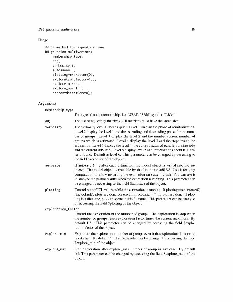
The type of node membership, i.e. ’SBM’, ’SBM_sym’ or ’LBM’
adj The adjacency matrix
verbosity The verbosity level, 0 means quiet. Level 1 display the phase of reinitialization.Level 2 display the level 1 and the ascending and descending phase for the num-ber of groups. Level 3 display the level 2 and the number current number ofgroups which is estimated. Level 4 display the level 3 and the steps inside theestimation. Level 5 display the level 4, the current status of parallel running jobsand the current sub-step. Level 6 display level 5 and informations about ICL cri-teria found. Default is level 6. This parameter can be changed by accessing tothe field $verbosity of the object.
autosave If autosave != ”, after each estimation, the model object is writed into file au-tosave . The model object is readable by the function readRDS . Use-it for longcomputation to allow restarting the estimation on system crash. You can use itto alanyze the partial results when the estimation is running. This parameter canbe changed by accessing to the field $autosave of the object.
plotting Control plot of ICL values while the estimation is running. If plotting==character(0)(the default), plots are done on screen, if plotting==”, no plot are done, if plot-ting is a filename, plots are done in this filename. This parameter can be changedby accessing the field $plotting of the object.
BM_bernoulli 3
exploration_factor
Control the exploration of the number of groups. The exploration is stop whenthe number of groups reach exploration factor times the current maximum. Bydefault 1.5. This parameter can be changed by accessing the field $explo-ration_factor of the object.
explore_min Explore to the explore_min number of groups even if the exploration_factor ruleis satisfied. By default 4. This parameter can be changed by accessing the field$explore_min of the object.
explore_max Stop exploration after explore_max number of group in any case. By defaultInf. This parameter can be changed by accessing the field $explore_max of theobject.
ncores Number of parallel jobs to launch different EM intializations. By default de-tectCores(). This parameter can be changed by accessing the field $ncores ofthe object. This parameters is used only on Linux. Parallism is disabled onother plateform. (Not working on Windows, not tested on Mac OS, not testedon *BSD.)
Examples
## Not run:
#### SBM##
## generation of one SBM networknpc <- 30 # nodes per classQ <- 3 # classesn <- npc * Q # nodesZ<-diag(Q)%x%matrix(1,npc,1)P<-matrix(runif(Q*Q),Q,Q)M<-1*(matrix(runif(n*n),n,n)<Z%*%P%*%t(Z)) ## adjacency matrix
The type of node membership, i.e. ’SBM’, ’SBM_sym’ or ’LBM’
adj The adjacency matrix
covariates Covariates matrix, or list of covariates matrices. Covariates matrix must havethe same size than the adjacency matrix.
verbosity The verbosity level, 0 means quiet. Level 1 display the phase of reinitialization.Level 2 display the level 1 and the ascending and descending phase for the num-ber of groups. Level 3 display the level 2 and the number current number ofgroups which is estimated. Level 4 display the level 3 and the steps inside theestimation. Level 5 display the level 4, the current status of parallel running jobsand the current sub-step. Level 6 display level 5 and informations about ICL cri-teria found. Default is level 6. This parameter can be changed by accessing tothe field $verbosity of the object.
autosave If autosave != ”, after each estimation, the model object is writed into file au-tosave . The model object is readable by the function readRDS . Use-it for longcomputation to allow restarting the estimation on system crash. You can use itto alanyze the partial results when the estimation is running. This parameter canbe changed by accessing to the field $autosave of the object.
plotting Control plot of ICL values while the estimation is running. If plotting==character(0)(the default), plots are done on screen, if plotting==”, no plot are done, if plot-ting is a filename, plots are done in this filename. This parameter can be changedby accessing the field $plotting of the object.
exploration_factor
Control the exploration of the number of groups. The exploration is stop whenthe number of groups reach exploration factor times the current maximum. Bydefault 1.5. This parameter can be changed by accessing the field $explo-ration_factor of the object.
explore_min Explore to the explore_min number of groups even if the exploration_factor ruleis satisfied. By default 4. This parameter can be changed by accessing the field$explore_min of the object.
explore_max Stop exploration after explore_max number of group in any case. By defaultInf. This parameter can be changed by accessing the field $explore_max of theobject.
ncores Number of parallel jobs to launch different EM intializations. By default de-tectCores(). This parameter can be changed by accessing the field $ncores ofthe object. This parameters is used only on Linux. Parallism is disabled onother plateform. (Not working on Windows, not tested on Mac OS, not testedon *BSD.)
Examples
## Not run:
#### SBM
6 BM_bernoulli_covariates
##
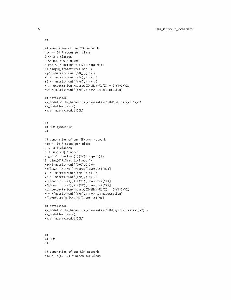
## generation of one SBM networknpc <- 30 # nodes per classQ <- 3 # classesn <- npc * Q # nodessigmo <- function(x){1/(1+exp(-x))}Z<-diag(Q)%x%matrix(1,npc,1)Mg<-8*matrix(runif(Q*Q),Q,Q)-4Y1 <- matrix(runif(n*n),n,n)-.5Y2 <- matrix(runif(n*n),n,n)-.5M_in_expectation<-sigmo(Z%*%Mg%*%t(Z) + 5*Y1-3*Y2)M<-1*(matrix(runif(n*n),n,n)<M_in_expectation)
The type of node membership, i.e. ’SBM’, ’SBM_sym’ or ’LBM’
adj The adjacency matrix
8 BM_bernoulli_covariates_fast
covariates Covariates matrix, or list of covariates matrices. Covariates matrix must havethe same size than the adjacency matrix.
verbosity The verbosity level, 0 means quiet. Level 1 display the phase of reinitialization.Level 2 display the level 1 and the ascending and descending phase for the num-ber of groups. Level 3 display the level 2 and the number current number ofgroups which is estimated. Level 4 display the level 3 and the steps inside theestimation. Level 5 display the level 4, the current status of parallel running jobsand the current sub-step. Level 6 display level 5 and informations about ICL cri-teria found. Default is level 6. This parameter can be changed by accessing tothe field $verbosity of the object.
autosave If autosave != ”, after each estimation, the model object is writed into file au-tosave . The model object is readable by the function readRDS . Use-it for longcomputation to allow restarting the estimation on system crash. You can use itto alanyze the partial results when the estimation is running. This parameter canbe changed by accessing to the field $autosave of the object.
plotting Control plot of ICL values while the estimation is running. If plotting==character(0)(the default), plots are done on screen, if plotting==”, no plot are done, if plot-ting is a filename, plots are done in this filename. This parameter can be changedby accessing the field $plotting of the object.
exploration_factor
Control the exploration of the number of groups. The exploration is stop whenthe number of groups reach exploration factor times the current maximum. Bydefault 1.5. This parameter can be changed by accessing the field $explo-ration_factor of the object.
explore_min Explore to the explore_min number of groups even if the exploration_factor ruleis satisfied. By default 4. This parameter can be changed by accessing the field$explore_min of the object.
explore_max Stop exploration after explore_max number of group in any case. By defaultInf. This parameter can be changed by accessing the field $explore_max of theobject.
ncores Number of parallel jobs to launch different EM intializations. By default de-tectCores(). This parameter can be changed by accessing the field $ncores ofthe object. This parameters is used only on Linux. Parallism is disabled onother plateform. (Not working on Windows, not tested on Mac OS, not testedon *BSD.)
Examples
## Not run:
#### SBM##
## generation of one SBM networknpc <- 30 # nodes per classQ <- 3 # classesn <- npc * Q # nodes
The type of node membership, i.e. ’SBM’, ’SBM_sym’ or ’LBM’
adj The list of adjacency matrices. All matrices must have the same size
verbosity The verbosity level, 0 means quiet. Level 1 display the phase of reinitialization.Level 2 display the level 1 and the ascending and descending phase for the num-ber of groups. Level 3 display the level 2 and the number current number ofgroups which is estimated. Level 4 display the level 3 and the steps inside theestimation. Level 5 display the level 4, the current status of parallel running jobsand the current sub-step. Level 6 display level 5 and informations about ICL cri-teria found. Default is level 6. This parameter can be changed by accessing tothe field $verbosity of the object.
BM_bernoulli_multiplex 11
autosave If autosave != ”, after each estimation, the model object is writed into file au-tosave . The model object is readable by the function readRDS . Use-it for longcomputation to allow restarting the estimation on system crash. You can use itto alanyze the partial results when the estimation is running. This parameter canbe changed by accessing to the field $autosave of the object.
plotting Control plot of ICL values while the estimation is running. If plotting==character(0)(the default), plots are done on screen, if plotting==”, no plot are done, if plot-ting is a filename, plots are done in this filename. This parameter can be changedby accessing the field $plotting of the object.
exploration_factor
Control the exploration of the number of groups. The exploration is stop whenthe number of groups reach exploration factor times the current maximum. Bydefault 1.5. This parameter can be changed by accessing the field $explo-ration_factor of the object.
explore_min Explore to the explore_min number of groups even if the exploration_factor ruleis satisfied. By default 4. This parameter can be changed by accessing the field$explore_min of the object.
explore_max Stop exploration after explore_max number of group in any case. By defaultInf. This parameter can be changed by accessing the field $explore_max of theobject.
ncores Number of parallel jobs to launch different EM intializations. By default de-tectCores(). This parameter can be changed by accessing the field $ncores ofthe object. This parameters is used only on Linux. Parallism is disabled onother plateform. (Not working on Windows, not tested on Mac OS, not testedon *BSD.)
The type of node membership, i.e. ’SBM’, ’SBM_sym’ or ’LBM’
adj The adjacency matrix
verbosity The verbosity level, 0 means quiet. Level 1 display the phase of reinitialization.Level 2 display the level 1 and the ascending and descending phase for the num-ber of groups. Level 3 display the level 2 and the number current number ofgroups which is estimated. Level 4 display the level 3 and the steps inside theestimation. Level 5 display the level 4, the current status of parallel running jobsand the current sub-step. Level 6 display level 5 and informations about ICL cri-teria found. Default is level 6. This parameter can be changed by accessing tothe field $verbosity of the object.
autosave If autosave != ”, after each estimation, the model object is writed into file au-tosave . The model object is readable by the function readRDS . Use-it for longcomputation to allow restarting the estimation on system crash. You can use itto alanyze the partial results when the estimation is running. This parameter canbe changed by accessing to the field $autosave of the object.
plotting Control plot of ICL values while the estimation is running. If plotting==character(0)(the default), plots are done on screen, if plotting==”, no plot are done, if plot-ting is a filename, plots are done in this filename. This parameter can be changedby accessing the field $plotting of the object.
exploration_factor
Control the exploration of the number of groups. The exploration is stop whenthe number of groups reach exploration factor times the current maximum. Bydefault 1.5. This parameter can be changed by accessing the field $explo-ration_factor of the object.
explore_min Explore to the explore_min number of groups even if the exploration_factor ruleis satisfied. By default 4. This parameter can be changed by accessing the field$explore_min of the object.
explore_max Stop exploration after explore_max number of group in any case. By defaultInf. This parameter can be changed by accessing the field $explore_max of theobject.
ncores Number of parallel jobs to launch different EM intializations. By default de-tectCores(). This parameter can be changed by accessing the field $ncores ofthe object. This parameters is used only on Linux. Parallism is disabled onother plateform. (Not working on Windows, not tested on Mac OS, not testedon *BSD.)
The type of node membership, i.e. ’SBM’, ’SBM_sym’ or ’LBM’
adj The adjacency matrix
covariates Covariates matrix, or list of covariates matrices. Covariates matrix must havethe same size than the adjacency matrix.
verbosity The verbosity level, 0 means quiet. Level 1 display the phase of reinitialization.Level 2 display the level 1 and the ascending and descending phase for the num-ber of groups. Level 3 display the level 2 and the number current number ofgroups which is estimated. Level 4 display the level 3 and the steps inside theestimation. Level 5 display the level 4, the current status of parallel running jobsand the current sub-step. Level 6 display level 5 and informations about ICL cri-teria found. Default is level 6. This parameter can be changed by accessing tothe field $verbosity of the object.
autosave If autosave != ”, after each estimation, the model object is writed into file au-tosave . The model object is readable by the function readRDS . Use-it for longcomputation to allow restarting the estimation on system crash. You can use itto alanyze the partial results when the estimation is running. This parameter canbe changed by accessing to the field $autosave of the object.
BM_gaussian_covariates 17
plotting Control plot of ICL values while the estimation is running. If plotting==character(0)(the default), plots are done on screen, if plotting==”, no plot are done, if plot-ting is a filename, plots are done in this filename. This parameter can be changedby accessing the field $plotting of the object.
exploration_factor
Control the exploration of the number of groups. The exploration is stop whenthe number of groups reach exploration factor times the current maximum. Bydefault 1.5. This parameter can be changed by accessing the field $explo-ration_factor of the object.
explore_min Explore to the explore_min number of groups even if the exploration_factor ruleis satisfied. By default 4. This parameter can be changed by accessing the field$explore_min of the object.
explore_max Stop exploration after explore_max number of group in any case. By defaultInf. This parameter can be changed by accessing the field $explore_max of theobject.
ncores Number of parallel jobs to launch different EM intializations. By default de-tectCores(). This parameter can be changed by accessing the field $ncores ofthe object. This parameters is used only on Linux. Parallism is disabled onother plateform. (Not working on Windows, not tested on Mac OS, not testedon *BSD.)
Examples
## Not run:
#### SBM##
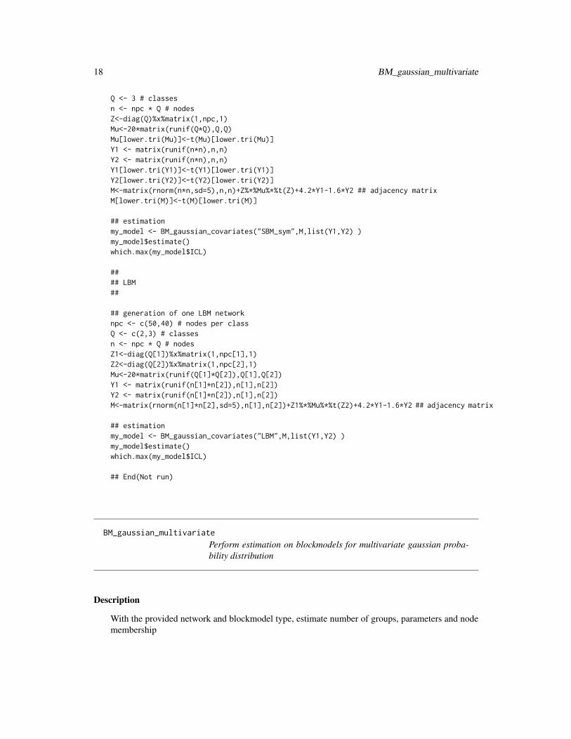
## generation of one SBM networknpc <- 30 # nodes per classQ <- 3 # classesn <- npc * Q # nodesZ<-diag(Q)%x%matrix(1,npc,1)Mu<-20*matrix(runif(Q*Q),Q,Q)Y1 <- matrix(runif(n*n),n,n)Y2 <- matrix(runif(n*n),n,n)M<-matrix(rnorm(n*n,sd=5),n,n)+Z%*%Mu%*%t(Z)+4.2*Y1-1.6*Y2 ## adjacency matrix
The type of node membership, i.e. ’SBM’, ’SBM_sym’ or ’LBM’
adj The list of adjacency matrices. All matrices must have the same size
verbosity The verbosity level, 0 means quiet. Level 1 display the phase of reinitialization.Level 2 display the level 1 and the ascending and descending phase for the num-ber of groups. Level 3 display the level 2 and the number current number ofgroups which is estimated. Level 4 display the level 3 and the steps inside theestimation. Level 5 display the level 4, the current status of parallel running jobsand the current sub-step. Level 6 display level 5 and informations about ICL cri-teria found. Default is level 6. This parameter can be changed by accessing tothe field $verbosity of the object.
autosave If autosave != ”, after each estimation, the model object is writed into file au-tosave . The model object is readable by the function readRDS . Use-it for longcomputation to allow restarting the estimation on system crash. You can use itto alanyze the partial results when the estimation is running. This parameter canbe changed by accessing to the field $autosave of the object.
plotting Control plot of ICL values while the estimation is running. If plotting==character(0)(the default), plots are done on screen, if plotting==”, no plot are done, if plot-ting is a filename, plots are done in this filename. This parameter can be changedby accessing the field $plotting of the object.
exploration_factor
Control the exploration of the number of groups. The exploration is stop whenthe number of groups reach exploration factor times the current maximum. Bydefault 1.5. This parameter can be changed by accessing the field $explo-ration_factor of the object.
explore_min Explore to the explore_min number of groups even if the exploration_factor ruleis satisfied. By default 4. This parameter can be changed by accessing the field$explore_min of the object.
explore_max Stop exploration after explore_max number of group in any case. By defaultInf. This parameter can be changed by accessing the field $explore_max of theobject.
20 BM_gaussian_multivariate
ncores Number of parallel jobs to launch different EM intializations. By default de-tectCores(). This parameter can be changed by accessing the field $ncores ofthe object. This parameters is used only on Linux. Parallism is disabled onother plateform. (Not working on Windows, not tested on Mac OS, not testedon *BSD.)
Examples
## Not run:
#### SBM##
## generation of one SBM networknpc <- 30 # nodes per classQ <- 3 # classesn <- npc * Q # nodesZ<-diag(Q)%x%matrix(1,npc,1)Mu1<-4*matrix(runif(Q*Q),Q,Q)Mu2<-4*matrix(runif(Q*Q),Q,Q)Noise1<-matrix(rnorm(n*n,sd=1),n,n)Noise2<-matrix(rnorm(n*n,sd=1),n,n)M1<- Z%*%Mu1%*%t(Z) + Noise1M2<- Z%*%Mu2%*%t(Z) + 10*Noise1 + Noise2
The type of node membership, i.e. ’SBM’, ’SBM_sym’ or ’LBM’
adj The list of adjacency matrices. All matrices must have the same size
verbosity The verbosity level, 0 means quiet. Level 1 display the phase of reinitialization.Level 2 display the level 1 and the ascending and descending phase for the num-ber of groups. Level 3 display the level 2 and the number current number ofgroups which is estimated. Level 4 display the level 3 and the steps inside theestimation. Level 5 display the level 4, the current status of parallel running jobsand the current sub-step. Level 6 display level 5 and informations about ICL cri-teria found. Default is level 6. This parameter can be changed by accessing tothe field $verbosity of the object.
autosave If autosave != ”, after each estimation, the model object is writed into file au-tosave . The model object is readable by the function readRDS . Use-it for longcomputation to allow restarting the estimation on system crash. You can use itto alanyze the partial results when the estimation is running. This parameter canbe changed by accessing to the field $autosave of the object.
plotting Control plot of ICL values while the estimation is running. If plotting==character(0)(the default), plots are done on screen, if plotting==”, no plot are done, if plot-ting is a filename, plots are done in this filename. This parameter can be changedby accessing the field $plotting of the object.
exploration_factor
Control the exploration of the number of groups. The exploration is stop whenthe number of groups reach exploration factor times the current maximum. Bydefault 1.5. This parameter can be changed by accessing the field $explo-ration_factor of the object.
explore_min Explore to the explore_min number of groups even if the exploration_factor ruleis satisfied. By default 4. This parameter can be changed by accessing the field$explore_min of the object.
explore_max Stop exploration after explore_max number of group in any case. By defaultInf. This parameter can be changed by accessing the field $explore_max of theobject.
ncores Number of parallel jobs to launch different EM intializations. By default de-tectCores(). This parameter can be changed by accessing the field $ncores ofthe object. This parameters is used only on Linux. Parallism is disabled onother plateform. (Not working on Windows, not tested on Mac OS, not testedon *BSD.)
The type of node membership, i.e. ’SBM’, ’SBM_sym’ or ’LBM’adj The list of adjacency matrices. All matrices must have the same sizeverbosity The verbosity level, 0 means quiet. Level 1 display the phase of reinitialization.
Level 2 display the level 1 and the ascending and descending phase for the num-ber of groups. Level 3 display the level 2 and the number current number ofgroups which is estimated. Level 4 display the level 3 and the steps inside theestimation. Level 5 display the level 4, the current status of parallel running jobsand the current sub-step. Level 6 display level 5 and informations about ICL cri-teria found. Default is level 6. This parameter can be changed by accessing tothe field $verbosity of the object.
autosave If autosave != ”, after each estimation, the model object is writed into file au-tosave . The model object is readable by the function readRDS . Use-it for longcomputation to allow restarting the estimation on system crash. You can use itto alanyze the partial results when the estimation is running. This parameter canbe changed by accessing to the field $autosave of the object.
plotting Control plot of ICL values while the estimation is running. If plotting==character(0)(the default), plots are done on screen, if plotting==”, no plot are done, if plot-ting is a filename, plots are done in this filename. This parameter can be changedby accessing the field $plotting of the object.
exploration_factor
Control the exploration of the number of groups. The exploration is stop whenthe number of groups reach exploration factor times the current maximum. Bydefault 1.5. This parameter can be changed by accessing the field $explo-ration_factor of the object.
explore_min Explore to the explore_min number of groups even if the exploration_factor ruleis satisfied. By default 4. This parameter can be changed by accessing the field$explore_min of the object.
explore_max Stop exploration after explore_max number of group in any case. By defaultInf. This parameter can be changed by accessing the field $explore_max of theobject.
ncores Number of parallel jobs to launch different EM intializations. By default de-tectCores(). This parameter can be changed by accessing the field $ncores ofthe object. This parameters is used only on Linux. Parallism is disabled onother plateform. (Not working on Windows, not tested on Mac OS, not testedon *BSD.)
Examples
## Not run:
#### SBM##
## generation of one SBM networknpc <- 30 # nodes per classQ <- 3 # classesn <- npc * Q # nodesZ<-diag(Q)%x%matrix(1,npc,1)Mu1<-4*matrix(runif(Q*Q),Q,Q)Mu2<-4*matrix(runif(Q*Q),Q,Q)M1<-matrix(rnorm(n*n,sd=5),n,n)+Z%*%Mu1%*%t(Z) ## adjacencyM2<-matrix(rnorm(n*n,sd=5),n,n)+Z%*%Mu2%*%t(Z) ## adjacency
The type of node membership, i.e. ’SBM’, ’SBM_sym’ or ’LBM’
adj The adjacency matrix
verbosity The verbosity level, 0 means quiet. Level 1 display the phase of reinitialization.Level 2 display the level 1 and the ascending and descending phase for the num-ber of groups. Level 3 display the level 2 and the number current number ofgroups which is estimated. Level 4 display the level 3 and the steps inside theestimation. Level 5 display the level 4, the current status of parallel running jobsand the current sub-step. Level 6 display level 5 and informations about ICL cri-teria found. Default is level 6. This parameter can be changed by accessing tothe field $verbosity of the object.
autosave If autosave != ”, after each estimation, the model object is writed into file au-tosave . The model object is readable by the function readRDS . Use-it for longcomputation to allow restarting the estimation on system crash. You can use itto alanyze the partial results when the estimation is running. This parameter canbe changed by accessing to the field $autosave of the object.
plotting Control plot of ICL values while the estimation is running. If plotting==character(0)(the default), plots are done on screen, if plotting==”, no plot are done, if plot-ting is a filename, plots are done in this filename. This parameter can be changedby accessing the field $plotting of the object.
exploration_factor
Control the exploration of the number of groups. The exploration is stop whenthe number of groups reach exploration factor times the current maximum. Bydefault 1.5. This parameter can be changed by accessing the field $explo-ration_factor of the object.
explore_min Explore to the explore_min number of groups even if the exploration_factor ruleis satisfied. By default 4. This parameter can be changed by accessing the field$explore_min of the object.
explore_max Stop exploration after explore_max number of group in any case. By defaultInf. This parameter can be changed by accessing the field $explore_max of theobject.
28 BM_poisson
ncores Number of parallel jobs to launch different EM intializations. By default de-tectCores(). This parameter can be changed by accessing the field $ncores ofthe object. This parameters is used only on Linux. Parallism is disabled onother plateform. (Not working on Windows, not tested on Mac OS, not testedon *BSD.)
Examples
## Not run:
## SBM#
## generation of one SBM networknpc <- 30 # nodes per classQ <- 3 # classesn <- npc * Q # nodesZ<-diag(Q)%x%matrix(1,npc,1)L<-70*matrix(runif(Q*Q),Q,Q)M_in_expectation<-Z%*%L%*%t(Z)M<-matrix(
The type of node membership, i.e. ’SBM’, ’SBM_sym’ or ’LBM’
adj The adjacency matrix
covariates Covariates matrix, or list of covariates matrices. Covariates matrix must havethe same size than the adjacency matrix.
verbosity The verbosity level, 0 means quiet. Level 1 display the phase of reinitialization.Level 2 display the level 1 and the ascending and descending phase for the num-ber of groups. Level 3 display the level 2 and the number current number ofgroups which is estimated. Level 4 display the level 3 and the steps inside theestimation. Level 5 display the level 4, the current status of parallel running jobsand the current sub-step. Level 6 display level 5 and informations about ICL cri-teria found. Default is level 6. This parameter can be changed by accessing tothe field $verbosity of the object.
autosave If autosave != ”, after each estimation, the model object is writed into file au-tosave . The model object is readable by the function readRDS . Use-it for longcomputation to allow restarting the estimation on system crash. You can use itto alanyze the partial results when the estimation is running. This parameter canbe changed by accessing to the field $autosave of the object.
plotting Control plot of ICL values while the estimation is running. If plotting==character(0)(the default), plots are done on screen, if plotting==”, no plot are done, if plot-ting is a filename, plots are done in this filename. This parameter can be changedby accessing the field $plotting of the object.
exploration_factor
Control the exploration of the number of groups. The exploration is stop whenthe number of groups reach exploration factor times the current maximum. Bydefault 1.5. This parameter can be changed by accessing the field $explo-ration_factor of the object.
explore_min Explore to the explore_min number of groups even if the exploration_factor ruleis satisfied. By default 4. This parameter can be changed by accessing the field$explore_min of the object.
explore_max Stop exploration after explore_max number of group in any case. By defaultInf. This parameter can be changed by accessing the field $explore_max of theobject.
ncores Number of parallel jobs to launch different EM intializations. By default de-tectCores(). This parameter can be changed by accessing the field $ncores ofthe object. This parameters is used only on Linux. Parallism is disabled onother plateform. (Not working on Windows, not tested on Mac OS, not testedon *BSD.)
BM_poisson_covariates 31
Examples
## Not run:
#### SBM##
## generation of one SBM networknpc <- 30 # nodes per classQ <- 3 # classesn <- npc * Q # nodesZ<-diag(Q)%x%matrix(1,npc,1)L<-70*matrix(runif(Q*Q),Q,Q)M_in_expectation_without_covariates<-Z%*%L%*%t(Z)Y1 <- matrix(runif(n*n),n,n)Y2 <- matrix(runif(n*n),n,n)M_in_expectation<-M_in_expectation_without_covariates*exp(4.2*Y1-1.2*Y2)M<-matrix(
## generation of one SBM_sym network, we re-use one produced for SBMnpc <- 30 # nodes per classQ <- 3 # classesn <- npc * Q # nodesZ<-diag(Q)%x%matrix(1,npc,1)L<-70*matrix(runif(Q*Q),Q,Q)L[lower.tri(L)]<-t(L)[lower.tri(L)]M_in_expectation_without_covariates<-Z%*%L%*%t(Z)Y1 <- matrix(runif(n*n),n,n)Y2 <- matrix(runif(n*n),n,n)Y1[lower.tri(Y1)]<-t(Y1)[lower.tri(Y1)]Y2[lower.tri(Y2)]<-t(Y2)[lower.tri(Y2)]M_in_expectation<-M_in_expectation_without_covariates*exp(4.2*Y1-1.2*Y2)M<-matrix(