Relativistic quantum transport coefficients for second-order viscous hydrodynamics

Wojciech Florkowski,1 Amaresh Jaiswal,2 Ewa Maksymiuk,1 Radoslaw Ryblewski,3 and Michael Strickland4

1Institute of Physics, Jan Kochanowski University, PL-25406 Kielce, Poland2GSI, Helmholtzzentrum fur Schwerionenforschung, Planckstrasse 1, D-64291 Darmstadt, Germany

3The H. Niewodniczanski Institute of Nuclear Physics,Polish Academy of Sciences, PL-31342 Krakow, Poland

4Department of Physics, Kent State University, Kent, Ohio 44242, USA(Dated: May 20, 2015)

We express the transport coefficients appearing in the second-order evolution equations for bulkviscous pressure and shear stress tensor using Bose-Einstein, Boltzmann, and Fermi-Dirac statisticsfor the equilibrium distribution function and Grad’s 14-moment approximation as well as the methodof Chapman-Enskog expansion for the non-equilibrium part. Specializing to the case of transversallyhomogeneous and boost-invariant longitudinal expansion of the viscous medium, we compare theresults obtained using the above methods with those obtained from the exact solution of the massive0+1d relativistic Boltzmann equation in the relaxation-time approximation. We show that comparedto the 14-moment approximation, the hydrodynamic transport coefficients obtained by employingthe Chapman-Enskog method leads to better agreement with the exact solution of the relativisticBoltzmann equation.

PACS numbers: 25.75.-q, 24.10.Nz, 47.75+f

I. INTRODUCTION

Relativistic viscous hydrodynamics has been appliedquite successfully to study and understand various collec-tive phenomena observed in the evolution of the stronglyinteracting QCD matter, with very high temperature anddensity, created in relativistic heavy-ion collisions; seeRef. [1] for a recent review. The derivation of hydrody-namic equations is essentially a coarse graining procedurewhereby one obtains an effective theory describing thelong-wavelength low-frequency limit of the microscopicdynamics of a system [1, 2]. Relativistic hydrodynamicsis formulated as an order-by-order expansion in powersof space-time gradients where ideal hydrodynamics is ofzeroth order [1]. The viscous effects arising in the first-order theory, also known as the relativistic Navier-Stokestheory [2, 3], results in acausal signal propagation andnumerical instability. While causality is restored in thesecond-order Israel-Stewart (IS) theory [4], stability maynot be guaranteed [5]. Consistent formulation of a causaltheory of relativistic viscous hydrodynamics and accuratedetermination of the associated transport coefficients iscurrently an active research topic [6–33].

The second-order IS equations can be derived in sev-eral ways [5]. For example, in the derivations based onthe second law of thermodynamics, the hydrodynamictransport coefficients related to the relaxation times forbulk and shear viscous evolution remain undetermined.While these transport coefficients can be obtained in thederivations based on kinetic theory [4, 6], the form of non-equilibrium phase-space distribution function, f(x, p),has to be specified. Two most extensively used meth-ods to determine f(x, p) for a system which is closeto local thermodynamic equilibrium are (1) the Grad’s14-moment approximation [34] and (2) the Chapman-Enskog method [35]. Note that while Grad’s 14-moment

approximation has been widely employed in the formu-lation of a causal theory of relativistic dissipative hydro-dynamics [4–14], the Chapman-Enskog method remainsless explored [15–19]. On the other hand, the Chapman-Enskog formalism has been often used to extract vari-ous transport coefficients of hot hadronic matter [20–24]Although in both methods the distribution function isexpanded around its equilibrium value f0(x, p), it hasbeen demonstrated that the Chapman-Enskog method inthe relaxation-time approximation (RTA) leads to betteragreement with both microscopic Boltzmann simulationsas well as exact solutions of the relativistic RTA Boltz-mann equation [16–19]. This may be attributed to thefact that a fixed-order moment expansion, as required inGrad’s approximation, is not necessary in the Chapman-Enskog method.

Much of the research on the application of viscous hy-drodynamics in relativistic heavy-ion collisions is devotedto the extraction of the shear viscosity to entropy den-sity ratio, η/s, from the analysis of the anisotropic flowdata [36–38]. Indeed the estimated η/s has been found tobe close to the conjectured lower bound η/s|KSS = 1/4π[39, 40]. On the other hand, a self-consistent and sys-tematic study of the effect of the bulk viscosity in nu-merical simulations of high-energy heavy-ion collisions isrelatively lacking. This may be attributed to the fact thatthe hot QCD matter is assumed to be nearly conformaland therefore the bulk viscosity is estimated to be muchsmaller compared to the shear viscosity. However, in re-ality, QCD is a non-conformal field theory and thereforebulk viscous corrections to the energy-momentum tensorshould not be ignored in order to correctly understandthe dynamics of the QCD system. Moreover, for therange of temperature explored in heavy-ion collision ex-periments at Relativistic Heavy-Ion Collider (RHIC) andLarge Hadron Collider (LHC), the magnitude and tem-

arX

iv:1

503.

0322

6v3

[nu

cl-t

h] 1

9 M

ay 2

015

2

perature dependence of the bulk viscosity could be largeenough to influence the space-time evolution of the hotQCD matter [41–47].

It is important to note that the second-order transportcoefficients, appearing in the evolution equation for thebulk viscous pressure, are less understood compared tothose of the shear stress tensor. While the relaxationtime for the bulk viscous evolution can be obtained byusing the second law of thermodynamics in a kinetictheory set up [11, 12], this method fails to account forthe important coupling of the bulk viscous pressure withthe shear stress tensor [13, 14, 18]. On the other hand,for finite masses and classical Boltzmann distribution,the second-order transport coefficients corresponding tobulk viscous pressure and shear stress tensor have beenobtained by employing the Grad’s 14-moment approxi-mation [13, 14] as well as the Chapman-Enskog method[18], within a purely kinetic theory framework. However,these transport coefficients still remain to be determinedfor quantum statistics, i.e., for Bose-Einstein and Fermi-Dirac distribution.

In this paper, we express the transport coefficients ap-pearing in the second-order viscous evolution equationswith non-vanishing masses for Bose-Einstein, Boltzmannand Fermi-Dirac distribution. We obtain these trans-port coefficients using the Grad’s 14-moment approxi-mation as well as the method of Chapman-Enskog ex-pansion. In addition, in the case of one-dimensionalscaling expansion of the viscous medium, we comparethe results obtained using the above methods with thoseobtained from the exact solution of massive 0+1d rel-ativistic Boltzmann equation in the relaxation-time ap-proximation [33]. We demonstrate that the results ob-tained using the Chapman-Enskog method are in bet-ter agreement with the exact solution of the RTA Boltz-mann equation than those obtained using the Grad’s 14-moment approximation.

II. RELATIVISTIC HYDRODYNAMICS

In the absence of any conserved charges, i.e., for van-ishing chemical potential, the hydrodynamic evolution ofa system is governed by the local conservation of energyand momentum: ∂µT

µν = 0. The energy-momentumtensor, Tµν , which characterizes the macroscopic state ofa system, can be expressed in terms of the single-particlephase-space distribution function, f(x, p), and tensor de-composed into hydrodynamic degrees of freedom [48],

Tµν =

∫dP pµpνf(x, p) = εuµuν − (P + Π)∆µν + πµν .

(1)Here dP ≡ gd3p/[(2π)3p0] is the invariant momentum-space integration measure, g being the degeneracy fac-tor, and pµ is the particle four-momentum. In the tensordecomposition, ε, P , Π, and πµν are the energy den-sity, the thermodynamic pressure, the bulk viscous pres-

sure, and the shear stress tensor, respectively. The pro-jection operator ∆µν ≡ gµν − uµuν is constructed suchthat it is orthogonal to the hydrodynamic four-velocityuµ. The metric tensor is assumed to be Minkowskian,gµν ≡ diag(+1,−1,−1,−1), and uµ is defined in the Lan-dau frame: Tµνuν = εuµ.

The energy-momentum conservation equation,∂µT

µν = 0, when projected along and orthogonal to uµ

gives the evolution equations for ε and uµ,

ε+ (ε+ P + Π)θ − πµνσµν = 0,

(ε+ P + Π)uα −∇α(P + Π) + ∆αν ∂µπ

µν = 0. (2)

Here we have used the usual notation θ ≡ ∂µuµ for the

expansion scalar, A ≡ uµ∂µA for the co-moving deriva-tive, ∇α ≡ ∆µα∂µ for the space-like derivative, andσµν ≡ (∇µuν + ∇νuµ)/2 − (θ/3)∆µν for the velocitystress tensor. The energy density and the thermody-namic pressure can be written in terms of the equilibriumphase-space distribution function f0 as

ε0 = uµuν

∫dP pµpνf0, (3)

P0 = −1

3∆µν

∫dP pµpνf0, (4)

where the equilibrium distribution function for vanishingchemical potential is given by

f0 =1

exp(βu · p) + a. (5)

Here u · p ≡ uµpµ and a = −1, 0, 1 for Bose-Einstein,

Boltzmann, and Fermi-Dirac gas, respectively. The in-verse temperature, β ≡ 1/T , is determined by the match-ing condition ε = ε0.

For a system close to local thermodynamic equilib-rium, the non-equilibrium phase-space distribution func-tion can be written as f = f0 + δf , where δf � f . UsingEq. (1), the bulk viscous pressure, Π, and the shear stresstensor, πµν , can be expressed in terms of δf as [48]

Π = −1

3∆αβ

∫dP pαpβ δf, (6)

πµν = ∆µναβ

∫dP pαpβ δf, (7)

where ∆µναβ ≡ (∆µ

α∆νβ + ∆µ

β∆να)/2 − (1/3)∆µν∆αβ is a

traceless symmetric projection operator orthogonal to uµ

and ∆µν . In the following, we employ the expressions forδf obtained using the Grad’s 14-moment approximationand the Chapman-Enskog like iterative solution of therelativistic Boltzmann equation to obtain expressions forthe quantum transport coefficients associated with vis-cous evolution.

III. VISCOUS CORRECTIONS TO THEDISTRIBUTION FUNCTION

Precise determination of the form of the non-equilibrium single particle phase-space distribution func-

3

tion is one of the central problems in statistical physics.For a system close to local thermodynamic equilibrium,the problem reduces to determining the form of the cor-rection to the equilibrium distribution function. Withinthe framework of relativistic hydrodynamics, the viscouscorrections to the equilibrium distribution function canbe obtained from two different methods: (1) the momentmethod and (2) the Chapman-Enskog method. The mo-ment method, more popularly known as the Grad’s 14-moment ansatz, is based on a Taylor-like expansion ofthe non-equilibrium distribution in powers of momenta.On the other hand, the Chapman-Enskog method relieson the solution of the Boltzmann equation.

Ignoring dissipation due to particle diffusion, theGrad’s 14-moment approximation leads to

δfG =[ {E0 +B0m

2 +D0(u · p)− 4B0(u · p)2}

Π

+B2pαpβπαβ

]f0f0, (8)

where f0 = 1− af0. The coefficients E0, B0, D0 and B2

are known in terms of m, T and u·p and can be expressedas

B2 =1

2J(0)42

, (9)

D0

3B0= 4

J(0)31 J

(0)20 − J

(0)41 J

(0)10

J(0)30 J

(0)10 − J

(0)20 J

(0)20

≡ C2, (10)

E0

3B0= m2 − 4

J(0)31 J

(0)30 − J

(0)41 J

(0)20

J(0)30 J

(0)10 − J

(0)20 J

(0)20

≡ C1, (11)

B0 = − 1

3C1J(0)21 + 3C2J

(0)31 − 3J

(0)41 + 5J

(0)42

, (12)

where the thermodynamic functions J(r)nq are defined as

J (r)nq ≡

1

(2q + 1)!!

∫dP (u · p)n−2q−r (∆µνp

µpν)qf0f0.

(13)In the above equation, the indices n− r and q representsthe number of times pµ and ∆µν appear in the integra-tion, respectively.

An analogous expression for δf can also be obtainedusing an iterative Chapman-Enskog like solution of therelativistic Boltzmann equation in the relaxation-timeapproximation [18, 49]. In absence of dissipation dueto particle diffusion, the Chapman-Enskog method leadsto [18]

δfCE =β

u · p

[− 1

3βΠ

{m2 − (1− 3c2s)(u · p)2

}Π

+1

2βπpµpνπµν

]f0f0, (14)

where

βΠ =5

3βπ − (ε+ P )c2s, (15)

βπ = β J(1)42 , (16)

and c2s ≡ dP/dε is the speed of sound squared which canbe expressed as

c2s =ε+ P

βJ(0)30

. (17)

IV. VISCOUS EVOLUTION EQUATIONS

The second-order evolution equations for Π and πµν

can be derived by considering the co-moving derivativeof Eqs. (6) and (7),

Π = −1

3∆αβ

∫dP pαpβ δf , (18)

π〈µν〉 = ∆µναβ

∫dP pαpβ δf . (19)

Further, δf appearing in the above equations can be sim-plified by rewriting the relativistic Boltzmann equation,

pµ∂µf = C[f ], (20)

in the form [9]

δf = −f0 −1

u · ppµ∇µf +

1

u · pC[f ]. (21)

In the following, we consider the relaxation-time approx-imation for the collision term in the Boltzmann equation,

C[f ] = − (u · p) δfτeq

, (22)

where τeq is the relaxation time. In general, in orderfor the collision term in the above equation to respectthe conservation of particle four-current and energy-momentum tensor, τeq must be independent of momentaand uµ has to be defined in the Landau frame [50].

Substituting δf from Eq. (21) into Eqs. (18) and (19)along with the form of δf given in Eqs. (8) and (14), andafter performing the integrations, we obtain

Π =− Π

τeq− βΠθ − δΠΠΠθ + λΠππ

µνσµν , (23)

π〈µν〉 =− πµν

τeq+ 2βπσ

µν + 2π〈µγ ων〉γ − δπππµνθ

− τπππ〈µγ σν〉γ + λπΠΠσµν , (24)

where ωµν ≡ 12 (∇µuν − ∇νuµ) is the vorticity tensor.

Note that the above form of the evolution equations forthe bulk viscous pressure and the shear stress tensoris exactly same for both Grad’s 14-moment approxima-tion (δfG) and the Chapman-Enskog expansion (δfCE).Moreover, the expressions for the first order transport co-efficients, βΠ and βπ, are also identical for these two casesand are given in Eqs. (15) and (16). However, the secondorder transport coefficients appearing in the above equa-tions are different for the Grad’s 14-moment method andthe Chapman-Enskog method.

4

The transport coefficients in the case of Grad’s 14-moment approximation are calculated to be

δ(G)ΠΠ = 1− c2s −

m4

9γ

(0)2 , (25)

λ(G)Ππ =

1

3− c2s +

m2

3γ

(2)2 , (26)

δ(G)ππ =

4

3+m2

3γ

(2)2 , (27)

τ (G)ππ =

10

7+

4m2

7γ

(2)2 , (28)

λ(G)πΠ =

6

5− 2m4

15γ

(0)2 , (29)

where

γ(0)2 = (E0 +B0m

2)J(0)−20 +D0J

(0)−10 − 4B0J

(0)00 , (30)

γ(2)2 =

J(0)22

J(0)42

. (31)

On the other hand, these transport coefficients in thecase of Chapman-Enskog method are obtained as

δ(CE)ΠΠ = −5

9χ− c2s, (32)

λ(CE)Ππ =

β

3βπ

(7J

(3)63 + 2J

(1)42

)− c2s, (33)

δ(CE)ππ =

5

3+

7β

3βπJ

(3)63 , (34)

τ (CE)ππ = 2 +

4β

βπJ

(3)63 , (35)

λ(CE)πΠ = −2

3χ, (36)

where

χ =β

βΠ

[(1− 3c2s)

(J

(1)42 + J

(0)31

)−m2

(J

(3)42 + J

(2)31

)].

(37)

The integral functions J(r)nq appearing in the expres-

sions for the transport coefficients satisfy the relations

J (r)nq =

1

(2q + 1)

[m2J

(r)n−2,q−1 − J

(r)n,q−1

], (38)

J (0)nq =

1

β

[−I(0)

n−1,q−1 + (n− 2q)I(0)n−1,q

], (39)

where,

I(r)nq ≡

1

(2q + 1)!!

∫dP (u · p)n−2q−r (∆µνp

µpν)qf0. (40)

Here we readily identify I(0)20 = ε and I

(0)21 = −P . Using

Eqs. (38) and (39), we obtain the identities

J(0)42 =

m2

5J

(0)21 −

1

5J

(0)41 , (41)

J(0)31 = − 1

β(ε+ P ). (42)

To compute all the transport coefficients, we also need to

determine the integrals J(0)20 , J

(0)10 , J

(0)41 , J

(0)21 , J

(0)30 , J

(0)−20,

J(0)−10, J

(0)00 , J

(0)22 , J

(3)63 , J

(1)42 , J

(3)42 , and J

(2)31 . In the follow-

ing, we obtain expressions for these quantities in termsof modified Bessel functions of the second kind.

V. TRANSPORT COEFFICIENTS

Let us first simplify our equilibrium distribution func-tion. Using the result of summation of a infinite geomet-ric progression,

1

1 + x= 1− x+ x2 − x3 · · · =

∞∑l=0

(−1)lxl, for |x| < 1,

(43)we obtain,

f0 =e−β(u·p)

1 + ae−β(u·p) =

∞∑l=1

(−a)l−1e−lβ(u·p). (44)

Similarly, using the result obtained after differentiatingEq. (43), we obtain

f0f0 =e−β(u·p)

(1 + ae−β(u·p))2=

∞∑l=1

l(−a)l−1e−lβ(u·p). (45)

Using the above results for f0 and f0f0, the thermody-

namic integrals I(r)nq and J

(r)nq can be written as,

I(r)nq =

gTn+2−rzn+2−r

2π2(2q + 1)!!(−1)q

∞∑l=1

(−a)l−1

∫ ∞0

dθ (46)

× (cosh θ)n−2q−r(sinh θ)2q+2 exp(−lz cosh θ),

J (r)nq =

gTn+2−rzn+2−r

2π2(2q + 1)!!(−1)q

∞∑l=1

l(−a)l−1

∫ ∞0

dθ (47)

× (cosh θ)n−2q−r(sinh θ)2q+2 exp(−lz cosh θ),

where z ≡ βm = m/T .

The integral coefficients I(r)nq and J

(r)nq can be expressed

in terms of modified Bessel functions of the second kind.The integral representation of the relevant Bessel func-tion is given by

Kn(z) =

∫ ∞0

dθ cosh(nθ) exp(−z cosh θ). (48)

The pressure, energy density and J(0)30 , required to calcu-

late the velocity of sound, can be expressed in terms of

5

Bessel functions using the above equation

P =gT 4z2

2π2

∞∑l=1

1

l2(−a)l−1K2(lz), (49)

ε =gT 4z3

2π2

∞∑l=1

1

l(−a)l−1K3(lz)− P, (50)

J(0)30 =

gT 5z5

32π2

∞∑l=1

l(−a)l−1[K5(lz) +K3(lz)− 2K1(lz)

].

(51)

The integral functions J(r)nq appearing in the transport

coefficients obtained using the Grad’s 14-moment methodcan be expressed as

J(0)21 =− gT 4z2

2π2

∞∑l=1

1

l(−a)l−1K2,

J(0)20 =

gT 4z3

2π2

∞∑l=1

(−a)l−1K3 + J(0)21 ,

J(0)10 =

gT 3z3

8π2

∞∑l=1

l(−a)l−1[K3 −K1

],

J(0)41 =− gT 6z6

192π2

∞∑l=1

l(−a)l−1[K6 − 2K4 −K2 + 2K0

],

J(0)−20 =

g

2π2

∞∑l=1

l(−a)l−1[K0 −Ki,2

],

J(0)−10 =

gTz

2π2

∞∑l=1

l(−a)l−1[K1 −Ki,1

],

J(0)22 =

gT 4z4

240π2

∞∑l=1

l(−a)l−1[K4 − 8K2 + 15K0 − 8Ki,2

],

J(0)00 =

gT 2z2

4π2

∞∑l=1

l(−a)l−1[K2 −K0

], (52)

where the (lz)-dependence of Kn and Ki,n is implic-itly understood. The integral functions appearing inthe transport coefficients obtained using the Chapman-Enskog method are

J(3)63 =− gT 5z5

3360π2

∞∑l=1

l(−a)l−1[K5 − 11K3 + 58K1

− 64Ki,1 + 16Ki,3

],

J(1)42 =

gT 5z5

480π2

∞∑l=1

l(−a)l−1[K5− 7K3+ 22K1− 16Ki,1

],

J(3)42 =

gT 3z3

120π2

∞∑l=1

l(−a)l−1[K3− 9K1+ 12Ki,1− 4Ki,3

],

J(2)31 =− gT 3z3

24π2

∞∑l=1

l(−a)l−1[K3 − 5K1 + 4Ki,1

]. (53)

Here the function Ki,n(lz) is defined by the integral

Ki,n(lz) =

∫ ∞0

dθ

(cosh θ)nexp(−lz cosh θ). (54)

Note that the subscript i in the above function is not anindex and just serves to distinguish it from the Besselfunctions. Ki,n satisfy the following recurrence relation:

d

dzKi,n(lz) = −lKi,n−1(lz), (55)

which can be expressed in the integral form:

Ki,n(lz) = Ki,n(0)− l∫ z

0

Ki,n−1(lz′)dz′. (56)

We observe that by matching Ki,0(lz) = K0(lz), theabove recursion relation can be used to evaluate Ki,n(lz)up to any n.

Armed with the above expressions for J(r)nq in terms

of series summation of the Bessel function, it is instruc-tive to calculate the ratio between the coefficient of bulkviscosity and shear viscosity. In the relaxation-time ap-proximation, this ratio is given by ζ/η = βΠ/βπ [13, 18].In the small-z approximation, using the series expansionof the Bessel functions in powers of z, we obtain

ζ

η= Γ

(1

3− c2s

)2

+O(z5), (57)

where Γ = 75 for Boltzmann distribution and Γ = 48for Fermi-Dirac distribution. However, in the case ofBose-Einstein distribution (remember a = −1), we getΓ = −15 + 36/(1 + a), and therefore it diverges as∼ 1/(1 + a) up to the leading-order. It is interestingto note that the above expression is similar to the wellknown relation, ζ/η = 15(1/3 − c2s)2, derived by Wein-berg [51]. The difference in the proportionality constantmay be attributed to the fact that here we have consid-ered a single component system whereas, motivated byapplications to cosmology, Weinberg considered a systemcomposed of mixture of radiation and matter.

In order to calculate ζ/η for the quark-gluon plasma(QGP), we need to provide appropriate degeneracy fac-

tors for the integral coefficients I(r)nq and J

(r)nq . For QGP,

these integral coefficients will transform as

I(r)nq → I(r)

nq |g=gq,a=1 + I(r)nq |g=gg,a=−1,

J (r)nq → J (r)

nq |g=gq,a=1 + J (r)nq |g=gg,a=−1, (58)

where gq and gg are the degeneracy factors correspondingto quarks and gluons respectively. These factors are givenas

gq = Ns ×Nqq ×NC ×Nf = 12Nf ,

gg = Ns ×(N2C − 1

)= 16, (59)

where Nf is the number of flavours, NC = 3 is the num-ber of colours, Ns = 2 corresponds to spin degrees andNqq = 2 denotes quark and anti-quark.

6

0.01 0.1 1 10

10

102

m�T

Ζ�Η

I1�3

-c s

2M2

QGP HNf =2LQGP HNf =3LBoltzmann statistics

Bose-Einstein statistics

Fermi-Dirac statistics

FIG. 1: (Color online) m/T dependence of the ratio ζ/ηscaled by (1/3 − c2s)

2 for Boltzmann (red solid line), Bose-Einstein (blue dashed line) and Fermi-Dirac (green dottedline) statistics. We also show results for two-flavor (browndashed-dotted line) and three-flavor QGP (purple dashed-dotted-dotted line). Thin horizontal black dashed lines cor-responds to constant values 75 and 48.

In Fig. 1, we show m/T dependence of the ratio ζ/ηscaled by (1/3−c2s)2 for various cases. We observe that inaccordance with the predictions from small-z expansion,Eq. (57), the curve for Boltzmann statistics (red solidline) and Fermi-Dirac statistics (green dotted line) satu-rates at 75 and 48 (thin horizontal black dashed lines),respectively, at small values of z. We also see that atvery small-z, Bose-Einstein statistics (blue dashed line)results in very large values of the scaled viscosity ratio(ζ/η)/(1/3−c2s)2 indicating divergence. We see that thisratio for the QGP is dominated by the Bose-Einsteinstatistics for two-flavor (brown dashed-dotted line) aswell as three-flavor QGP (purple dashed-dotted-dottedline). This however does not imply that the bulk viscos-ity of QGP is very large because a realistic calculationwith lattice QCD equation of state suggest that z > 0.6even for temperatures as high as central RHIC and LHCenergies [49, 52, 53]. Moreover, for large-z we see thatall three statistics lead to similar results for the scaledviscosity ratio which suggests that there is a relativelysmall effect coming from composition of the fluid.

VI. BOOST-INVARIANT 0+1D CASE

In this section, we consider evolution in the case oftransversely homogeneous and purely-longitudinal boost-invariant expansion [54]. For such an expansion allscalar functions of space and time depend only on thelongitudinal proper time τ =

√t2 − z2. Working in

the Milne coordinate system, (τ, x, y, η), the hydrody-namic four-velocity is given by uµ = (1, 0, 0, 0). Theenergy-momentum conservation equation together with

-0.020

-0.015

-0.010

-0.005

0.000

0.005

-0.020

-0.015

-0.010

-0.005

0.000

0.005

ΤP

@fm-

3D

Boltzmann statisticsΞ0=0, Τ0=0.5fm, Τeq=0.25fm

T0=300MeV, m=300MeV

0.5 1 2 3 4 5 7 100.990

0.992

0.994

0.996

0.998

1.000

0.990

0.992

0.994

0.996

0.998

1.000

Τ @fm�cD

PL

�PT

HPL

�PT

L EX

AC

T

ExactChapman-EnskogGrad's 14-moment

FIG. 2: (Color online) Time evolution of the the bulk viscouspressure times τ (top) and the pressure anisotropy PL/PTscaled by that obtained using exact solution of the RTA Boltz-mann equation (bottom) for Boltzmann statistics. The threecurves in both panels correspond to three different calcula-tions: the exact solution of the RTA Boltzmann equation [33](red solid line), second-order viscous hydrodynamics obtainedusing the Chapman-Enskog method (blue dashed line) and us-ing the Grad’s 14-moment approximation (green dotted line).For both panels we use T0 = 300 MeV at τ0 = 0.5 fm/c,m = 300 MeV, and τeq = τπ = τΠ = 0.25 fm/c. The initialspheroidal anisotropy in the distribution function, ξ0 = 0,corresponds to isotropic initial pressures with Π0 = π0 = 0.

Eqs. (23) and (24) reduce to

ε = −1

τ(ε+ P + Π− π) , (60)

Π +Π

τΠ= −βΠ

τ− δΠΠ

Π

τ+ λΠπ

π

τ, (61)

π +π

τπ=

4

3

βπτ−(

1

3τππ + δππ

)π

τ+

2

3λπΠ

Π

τ, (62)

where π ≡ −τ2πηη. Note that in this case the terminvolving the vorticity tensor in Eq. (24) vanishes andhence has no effect on the dynamics of the fluid. Alsonote that the first terms on the right-hand side ofEqs. (61) and (62) corresponds to the first-order termsβΠθ and 2βπσ

µν , respectively, whereas the rest are ofsecond-order.

We simultaneously solve Eqs. (60)-(62) assuming aninitial temperature of T0 = 300 MeV at the initial propertime τ0 = 0.5 fm/c, with relaxation times τeq = τΠ =τπ = 0.25 fm/c corresponding to initial η/s = 1/4π.We solve these equations for two different initial pres-sure configurations: ξ0 = 0 corresponding to an isotropicpressure configuration π0 = Π0 = 0 and ξ0 = 100 cor-responding to a highly oblate anisotropic pressure con-figuration. The anisotropy parameter ξ is related to theaverage longitudinal and transverse momentum in the

7

-0.020

-0.015

-0.010

-0.005

0.000

0.005

-0.020

-0.015

-0.010

-0.005

0.000

0.005

ΤP

@fm-

3D

Bose-Einstein statisticsΞ0=0, Τ0=0.5fm, Τeq=0.25fm

T0=300MeV, m=300MeV

0.5 1 2 3 4 5 7 100.990

0.992

0.994

0.996

0.998

1.000

0.990

0.992

0.994

0.996

0.998

1.000

Τ @fm�cD

PL

�PT

HPL

�PT

L EX

AC

T

ExactChapman-EnskogGrad's 14-moment

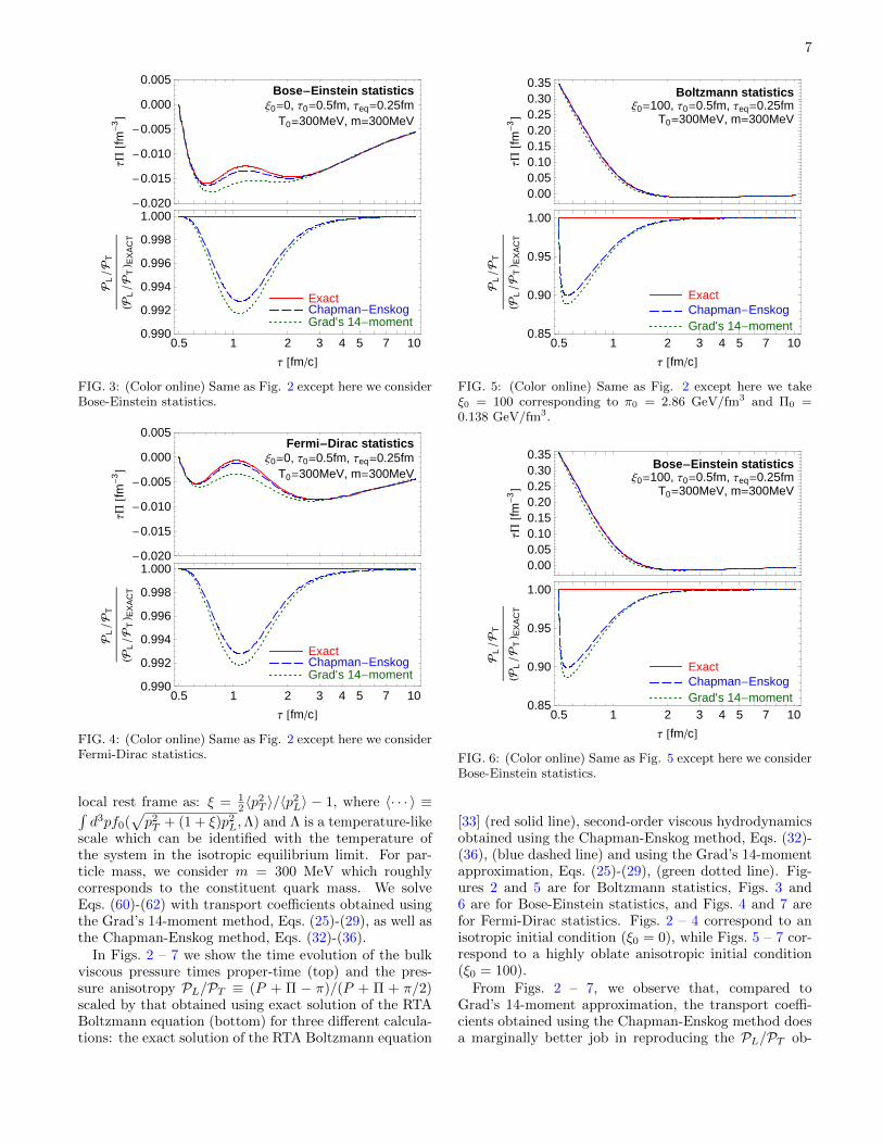
FIG. 3: (Color online) Same as Fig. 2 except here we considerBose-Einstein statistics.

-0.020

-0.015

-0.010

-0.005

0.000

0.005

-0.020

-0.015

-0.010

-0.005

0.000

0.005

ΤP

@fm-

3D

Fermi-Dirac statisticsΞ0=0, Τ0=0.5fm, Τeq=0.25fm

T0=300MeV, m=300MeV

0.5 1 2 3 4 5 7 100.990

0.992

0.994

0.996

0.998

1.000

0.990

0.992

0.994

0.996

0.998

1.000

Τ @fm�cD

PL

�PT

HPL

�PT

L EX

AC

T

ExactChapman-EnskogGrad's 14-moment

FIG. 4: (Color online) Same as Fig. 2 except here we considerFermi-Dirac statistics.

local rest frame as: ξ = 12 〈p

2T 〉/〈p2

L〉 − 1, where 〈· · · 〉 ≡∫d3pf0(

√p2T + (1 + ξ)p2

L,Λ) and Λ is a temperature-likescale which can be identified with the temperature ofthe system in the isotropic equilibrium limit. For par-ticle mass, we consider m = 300 MeV which roughlycorresponds to the constituent quark mass. We solveEqs. (60)-(62) with transport coefficients obtained usingthe Grad’s 14-moment method, Eqs. (25)-(29), as well asthe Chapman-Enskog method, Eqs. (32)-(36).

In Figs. 2 – 7 we show the time evolution of the bulkviscous pressure times proper-time (top) and the pres-sure anisotropy PL/PT ≡ (P + Π − π)/(P + Π + π/2)scaled by that obtained using exact solution of the RTABoltzmann equation (bottom) for three different calcula-tions: the exact solution of the RTA Boltzmann equation

0.000.050.100.150.200.250.300.35

0.00

0.05

0.10

0.15

0.20

0.25

0.30

0.35

ΤP

@fm-

3D

Boltzmann statisticsΞ0=100, Τ0=0.5fm, Τeq=0.25fm

T0=300MeV, m=300MeV

0.5 1 2 3 4 5 7 100.85

0.90

0.95

1.00

0.85

0.90

0.95

1.00

Τ @fm�cD

PL

�PT

HPL

�PT

L EX

AC

T

ExactChapman-EnskogGrad's 14-moment

FIG. 5: (Color online) Same as Fig. 2 except here we takeξ0 = 100 corresponding to π0 = 2.86 GeV/fm3 and Π0 =0.138 GeV/fm3.

0.000.050.100.150.200.250.300.35

0.00

0.05

0.10

0.15

0.20

0.25

0.30

0.35

ΤP

@fm-

3D

Bose-Einstein statisticsΞ0=100, Τ0=0.5fm, Τeq=0.25fm

T0=300MeV, m=300MeV

0.5 1 2 3 4 5 7 100.85

0.90

0.95

1.00

0.85

0.90

0.95

1.00

Τ @fm�cD

PL

�PT

HPL

�PT

L EX

AC

T

ExactChapman-EnskogGrad's 14-moment

FIG. 6: (Color online) Same as Fig. 5 except here we considerBose-Einstein statistics.

[33] (red solid line), second-order viscous hydrodynamicsobtained using the Chapman-Enskog method, Eqs. (32)-(36), (blue dashed line) and using the Grad’s 14-momentapproximation, Eqs. (25)-(29), (green dotted line). Fig-ures 2 and 5 are for Boltzmann statistics, Figs. 3 and6 are for Bose-Einstein statistics, and Figs. 4 and 7 arefor Fermi-Dirac statistics. Figs. 2 – 4 correspond to anisotropic initial condition (ξ0 = 0), while Figs. 5 – 7 cor-respond to a highly oblate anisotropic initial condition(ξ0 = 100).

From Figs. 2 – 7, we observe that, compared toGrad’s 14-moment approximation, the transport coeffi-cients obtained using the Chapman-Enskog method doesa marginally better job in reproducing the PL/PT ob-

8

0.000.050.100.150.200.250.300.35

0.00

0.05

0.10

0.15

0.20

0.25

0.30

0.35

ΤP

@fm-

3D

Fermi-Dirac statisticsΞ0=100, Τ0=0.5fm, Τeq=0.25fm

T0=300MeV, m=300MeV

0.5 1 2 3 4 5 7 100.85

0.90

0.95

1.00

0.85

0.90

0.95

1.00

Τ @fm�cD

PL

�PT

HPL

�PT

L EX

AC

T

ExactChapman-EnskogGrad's 14-moment

FIG. 7: (Color online) Same as Fig. 5 except here we considerFermi-Dirac statistics.

tained using the exact solution of the RTA Boltzmannequation. On the other hand, the result for τΠ ob-tained using the Chapman-Enskog method shows betteragreement with the exact solution of the RTA Boltzmannequation than the Grad’s 14-moment method.

VII. CONCLUSIONS AND OUTLOOK

In this paper we expressed the transport coefficientsappearing in the second-order viscous hydrodynamicalevolution of a massive gas using Bose-Einstein, Boltz-mann and Fermi-Dirac statistics for the equilibrium dis-tribution function and Grad’s 14-moment approximationas well as the method of Chapman-Enskog expansion forthe non-equilibrium part. The second-order viscous evo-lution equations are obtained by coarse graining the rel-ativistic Boltzmann equation in the relaxation-time ap-proximation. We also obtained the ratio of the coeffi-cient of bulk viscosity to that of shear viscosity, in termsof the speed of sound, for classical and quantum statis-tics as well as for the QGP. We then considered the spe-cific case of a transversally homogeneous and longitudi-

nally boost-invariant system for which it is possible toexactly solve the RTA Boltzmann equation [33]. Usingthis solution as a benchmark, we compared the pressureanisotropy and bulk viscous pressure evolution obtainedby employing both the Chapman-Enskog method as wellas the Grad’s 14-moment method. We demonstrated thatthe Chapman-Enskog method is in better agreement withthe exact solution of the RTA Boltzmann equation com-pared to the Grad’s 14-moment method. We found that,while both methods give similar results for the pressureanisotropy, the Chapman-Enskog method better repro-duces the exact solution for the bulk viscous pressureevolution.

At this juncture, we would like to clarify that we haveused the exact solution of the Boltzmann equation, in therelaxation-time approximation, as a benchmark in orderto compare different hydrodynamic formulations. Therelaxation-time approximation is based on the assump-tion that the collisions tend to restore the phase-spacedistribution function to its equilibrium value exponen-tially. Although the microscopic interactions of the con-stituent particles are not captured in this approximation,it is reasonably accurate to describe a system which isclose to local thermodynamic equilibrium [55]. Lookingforward, it will be interesting to determine the impact ofthe quantum transport coefficients, obtained herein, inhigher dimensional simulations. Moreover, it would alsobe instructive to see if the second-order results derivedherein could be extended to obtain third order transportcoefficients for quantum statistics [17]. We leave thesequestions for a future work.

Acknowledgments

A.J. acknowledges useful discussions with GabrielDenicol, Bengt Friman and Krzysztof Redlich. W.F. andE.M. were supported by Polish National Science CenterGrant No. DEC-2012/06/A/ST2/00390. A.J. was sup-ported by the Frankfurt Institute for Advanced Studies(FIAS). R.R. was supported by Polish National ScienceCenter Grant No. DEC-2012/07/D/ST2/02125. M.S.was supported in part by U.S. DOE Grant No. DE-SC0004104.

[1] U. Heinz and R. Snellings, Ann. Rev. Nucl. Part. Sci. 63,123 (2013).

[2] L.D. Landau and E.M. Lifshitz, Fluid Mechanics(Butterworth-Heinemann, Oxford, 1987).

[3] C. Eckart, Phys. Rev. 58, 267 (1940).[4] W. Israel and J. M. Stewart, Annals Phys. (N.Y.) 118,

341 (1979).[5] P. Romatschke, Int. J. Mod. Phys. E 19, 1 (2010).[6] A. Muronga, Phys. Rev. C 69, 034903 (2004).[7] A. El, Z. Xu and C. Greiner, Phys. Rev. C 81, 041901(R)

(2010).[8] G. S. Denicol, H. Niemi, E. Molnar and D. H. Rischke,

Phys. Rev. D 85, 114047 (2012).[9] G. S. Denicol, T. Koide and D. H. Rischke, Phys. Rev.

Lett. 105, 162501 (2010).[10] A. Jaiswal, R. S. Bhalerao and S. Pal, Phys. Lett. B

720, 347 (2013); J. Phys. Conf. Ser. 422, 012003 (2013);arXiv:1303.1892 [nucl-th].

[11] A. Jaiswal, R. S. Bhalerao and S. Pal, Phys. Rev. C 87,021901(R) (2013).

9

[12] R. S. Bhalerao, A. Jaiswal, S. Pal and V. Sreekanth,Phys. Rev. C 88, 044911 (2013).

[13] G. S. Denicol, S. Jeon and C. Gale, Phys. Rev. C 90,024912 (2014).

[14] G. S. Denicol, W. Florkowski, R. Ryblewski andM. Strickland, Phys. Rev. C 90, 044905 (2014).

[15] R. S. Bhalerao, A. Jaiswal, S. Pal and V. Sreekanth,Phys. Rev. C 89, 054903 (2014).

[16] A. Jaiswal, Phys. Rev. C 87, 051901(R) (2013);arXiv:1408.0867 [nucl-th].

[17] A. Jaiswal, Phys. Rev. C 88, 021903(R) (2013); Nucl.Phys. A 931, 1205 (2014).

[18] A. Jaiswal, R. Ryblewski and M. Strickland, Phys. Rev.C 90, 044908 (2014).

[19] C. Chattopadhyay, A. Jaiswal, S. Pal and R. Ryblewski,Phys. Rev. C 91, 024917 (2015).

[20] M. Prakash, M. Prakash, R. Venugopalan and G. Welke,Phys. Rept. 227, 321 (1993).

[21] D. Davesne, Phys. Rev. C 53, 3069 (1996).[22] A. Wiranata and M. Prakash, Phys. Rev. C 85, 054908

(2012).[23] A. Wiranata, M. Prakash and P. Chakraborty, Central

Eur. J. Phys. 10, 1349 (2012).[24] A. Wiranata, M. Prakash, P. Huovinen, V. Koch and

X. N. Wang, J. Phys. Conf. Ser. 535, 012017 (2014).[25] P. Romatschke and M. Strickland, Phys. Rev. D 68,

036004 (2003).[26] W. Florkowski and R. Ryblewski, Phys. Rev. C 83,

034907 (2011).[27] M. Martinez and M. Strickland, Nucl. Phys. A 848, 183

(2010).[28] W. Florkowski, R. Ryblewski and M. Strickland, Nucl.

Phys. A 916, 249 (2013); Phys. Rev. C 88, (2013)024903.

[29] D. Bazow, U. W. Heinz and M. Strickland, Phys. Rev. C90, 054910 (2014).

[30] M. Nopoush, R. Ryblewski and M. Strickland, Phys. Rev.C 90, 014908 (2014).

[31] W. Florkowski, R. Ryblewski, M. Strickland and L. Tinti,Phys. Rev. C 89, 054909 (2014).

[32] W. Florkowski, E. Maksymiuk, R. Ryblewski andM. Strickland, Phys. Rev. C 89, 054908 (2014).

[33] W. Florkowski and E. Maksymiuk, J. Phys. G 42, 045106(2015).

[34] H. Grad, Comm. Pure Appl. Math. 2, 331 (1949).[35] S. Chapman and T. G. Cowling, The Mathematical The-

ory of Non-uniform Gases (Cambridge University Press,Cambridge, 1970), 3rd ed.

[36] P. Romatschke and U. Romatschke, Phys. Rev. Lett. 99,172301 (2007).

[37] H. Song, S. A. Bass, U. Heinz, T. Hirano and C. Shen,Phys. Rev. Lett. 106, 192301 (2011) [Erratum-ibid. 109,139904 (2012)].

[38] B. Schenke, S. Jeon and C. Gale, Phys. Rev. C 85, 024901(2012).

[39] G. Policastro, D. T. Son and A. O. Starinets, Phys. Rev.Lett. 87, 081601 (2001).

[40] P. Kovtun, D. T. Son and A. O. Starinets, Phys. Rev.Lett. 94, 111601 (2005).

[41] S. Gavin, Nucl. Phys. A 435, 826 (1985).[42] G. D. Moore and O. Saremi, JHEP 0809, 015 (2008).[43] A. Wiranata and M. Prakash, Nucl. Phys. A 830, 219C

(2009).[44] P. Chakraborty and J. I. Kapusta, Phys. Rev. C 83,

014906 (2011).[45] J. Noronha-Hostler, J. Noronha and F. Grassi, Phys.

Rev. C 90, 034907 (2014).[46] J. B. Rose, J. F. Paquet, G. S. Denicol, M. Luzum,

B. Schenke, S. Jeon and C. Gale, Nucl. Phys. A 931,926 (2014).

[47] S. Ryu, J.-F. Paquet, C. Shen, G. S. Denicol, B. Schenke,S. Jeon and C. Gale, arXiv:1502.01675 [nucl-th].

[48] S.R. de Groot, W.A. van Leeuwen, and Ch.G. van Weert,Relativistic Kinetic Theory: Principles and Applications(North-Holland, Amsterdam, 1980).

[49] P. Romatschke, Phys. Rev. D 85, 065012 (2012).[50] J. L. Anderson and H. R. Witting Physica 74, 466 (1974).[51] S. Weinberg, Gravitation and Cosmology (Wiley, 1972);

Astrophys. J. 168, 175 (1971).[52] J. O. Andersen, L. E. Leganger, M. Strickland and N. Su,

JHEP 1108, 053 (2011).[53] M. Strickland, J. O. Andersen, A. Bandyopadhyay,

N. Haque, M. G. Mustafa and N. Su, Nucl. Phys. A 931,841 (2014).

[54] J. D. Bjorken, Phys. Rev. D 27, 140 (1983).[55] K. Dusling, G. D. Moore and D. Teaney, Phys. Rev. C

81, 034907 (2010).