52
Pair-wise Sequence Alignment (II) Introduction to bioinformatics 2008 Lecture 6 C E N T R F O R I N T E G R A T I V E B I O I N F O R M A T I C S V U E
| Date post: | 26-Dec-2015 |
| Category: |
Documents |
| Upload: | jasmin-small |
| View: | 216 times |
| Download: | 3 times |

Pair-wise Sequence Alignment (II)
Introduction to bioinformatics 2008
Lecture 6
CENTR
FORINTEGRATIVE
BIOINFORMATICSVU
E

What can sequence alignment tell us about structure
HSSP Sander & Schneider, 1991
≥30% sequence identity

Sequence alignmentHistory of Dynamic
Programming algorithm
1970 Needleman-Wunsch global pair-wise alignment
Needleman SB, Wunsch CD (1970) A general method applicable to the search for similarities in the amino acid sequence of two proteins, J Mol Biol. 48(3):443-53.
1981 Smith-Waterman local pair-wise alignment
Smith, TF, Waterman, MS (1981) Identification of common molecular subsequences. J. Mol. Biol. 147, 195-197.

Global dynamic programming
i-1i
j-1 j
H(i,j) = Max H(i-1,j-1) + S(i,j)H(i-1,j) - gH(i,j-1) - g
diagonalverticalhorizontal
Value from residue exchange matrix
This is a recursive formula

Dynamic programming
i
j
The cell [i, j] contains the alignment score of the best scoring alignment score of subsequence 1..i and 1..j, that is, the subsequences up to [i, j]
Cell [i, j] does not ‘know’ what that best scoring alignment is (it is one out of many possibilities)
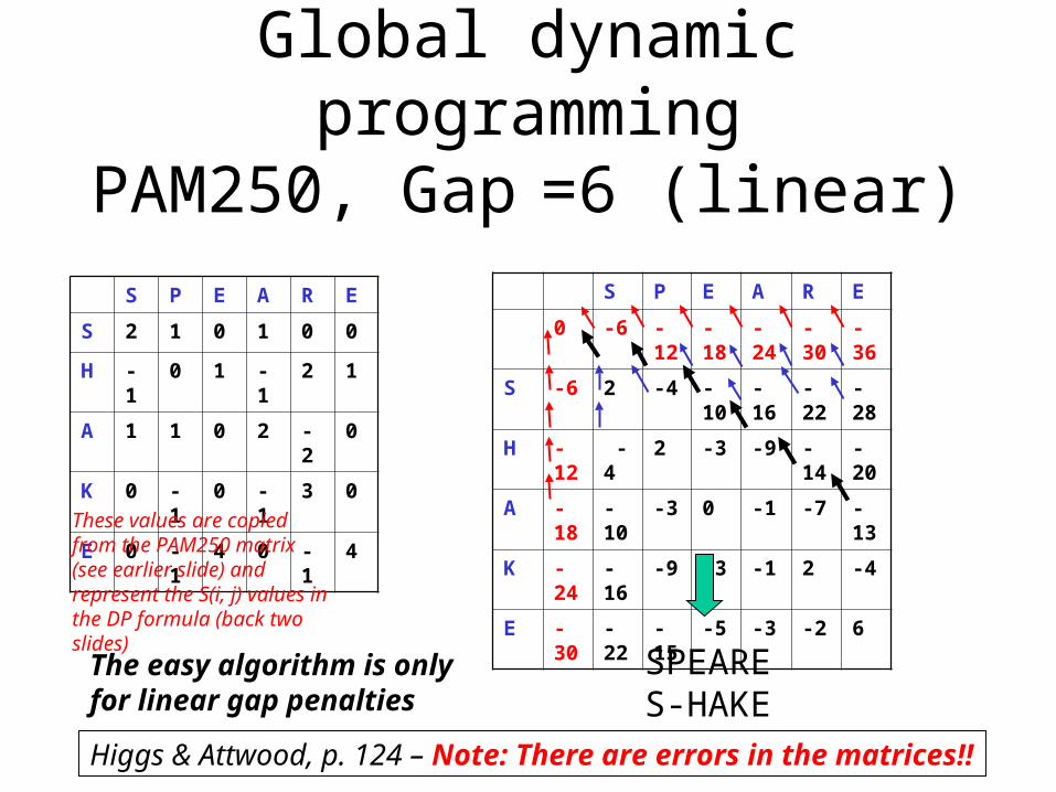
Global dynamic programmingPAM250, Gap =6 (linear)
S P E A R E
0 -6 -12 -18 -24 -30 -36
S -6 2 -4 -10 -16 -22 -28
H -12 -4 2 -3 -9 -14 -20
A -18 -10 -3 0 -1 -7 -13
K -24 -16 -9 -3 -1 2 -4
E -30 -22 -15 -5 -3 -2 6
S P E A R E
S 2 1 0 1 0 0
H -1 0 1 -1 2 1
A 1 1 0 2 -2 0
K 0 -1 0 -1 3 0
E 0 -1 4 0 -1 4
These values are copied from the PAM250 matrix (see earlier slide) and represent the S(i, j) values in the DP formula (back two slides)
Higgs & Attwood, p. 124 – Note: There are errors in the matrices!!
SPEARES-HAKE
The easy algorithm is only for linear gap penalties

Global dynamic programmingPAM250, Gap =6 (linear)
S P E A R E
0 -6 -12 -18 -24 -30 -36
S -6 2 -4 -10 -16 -22 -28
H -12 -4 2 -3 -9 -14 -20
A -18 -10 -3 2 -1 -7 -13
K -24 -16 -9 -3 1 2 -4
E -30 -22 -15 -5 -3 -2 6
S P E A R E
S 2 1 0 1 0 0
H -1 0 1 -1 2 1
A 1 1 0 2 -2 0
K 0 -1 0 -1 3 0
E 0 -1 4 0 -1 4
These values are copied from the PAM250 matrix (see earlier slide)
Higgs & Attwood, p. 124 – Note: There are errors in the matrices!!
SPEARES-HAKE
The easy algorithm is only for linear gap penalties
Start in left upper cell before either sequence (circled in red). Path will end in lower right cell (circled in blue)

DP is a two-step process
• Forward step: calculate scores • Trace back: start at highest score and
reconstruct the path leading to the highest score– These two steps lead to the highest
scoring alignment (the optimal alignment)
– This is guaranteed when you use DP!

Global dynamic programming
i-1i
j-1 j
H(i,j) = Max H(i-1,j-1) + S(i,j)H(i-1,j) - gH(i,j-1) - g
diagonalverticalhorizontal
Problem with simple DP approach:
•Can only do linear gap penalties
•Not suitable for affine and concave penalties, but algorithm can be extended to deal with affine penalties (preceding lecture)

Global dynamic programmingusing affine penalties
i-2i-1i
j-2 j-1 j
If you came from here, gap was opened so apply gap-open penalty
If you came from here, gap was already open, so apply gap-extension penalty
Looking back from cell (i, j) we can adapt the algorithm for affine gap penalties by looking back to four more cells (magenta)

Time and memory complexity of DP
• The time complexity is O(n2): if you would align two sequences of n residues, you would need to perform n2 algorithmic steps (square search matrix has n2 cells that need to be filled)
• The memory (space) complexity is also O(n2): if you would align two sequences of n residues, you would need a square search matrix of n by n containing n2 cells

Global dynamic programmingall types of gap penalties
i-1
j-1
Si,j = si,j + Max Max{S0<x<i-1, j-1 - Gap(i-x-1)}
Si-1,j-1
Max{Si-1, 0<y<j-1 - Gap(j-y-1)}
The complexity of this DP algorithm is increased from O(n2) to O(n3)
The gap length is known exactly and so any gap penalty regime can be used

Global dynamic programmingif affine penalties are used
i-1
j-1
Si,j = si,j + Max Max{S0<x<i-1, j-1 -Go -(i-x-1)*Ge}
Si-1,j-1
Max{Si-1, 0<y<j-1 -Go -(j-y-1)*Ge}

DP recipe for using affine gap penalties
• M[i,j] is optimal alignment (highest scoring alignment until [i,j])• Check
– preceding row until j-2: apply appropriate score and gap penalties– preceding row until i-2: apply appropriate score and gap penalties– and cell[i-1, j-1]: apply score for cell[i-1, j-1]
i-1
j-1

Global dynamic programmingAffine penalties: Gapo=10,
Gape=2D W V T A L K
0 -12 -14 -16 -18 -20 -22 -24
T -12 8 -9 -6 -5 -9 -11 -14
D -14 0 9 2 2 3 -5 -3 -34
W -16 -13 25 11 5 4 9 0 -21
V -18 -10 -4 37 21 19 19 15 -16
L -20 -14 -2 23 46 31 37 26 1
K -22 -12 -9 17 33 53 39 50 14
-34 -29 -1 17 39 27 50
D W V T A L K
T 8 3 8 11 9 9 8
D 12 1 6 8 8 4 8
W 1 25 2 3 2 6 5
V 6 2 12 8 8 10 6
L 4 6 10 9 6 14 5
K 8 5 6 8 7 5 13
These values are copied from the PAM250 matrix (see earlier slide), after being made non-negative by adding 8 to each PAM250 matrix cell (-8 is the lowest number in the PAM250 matrix)
The extra bottom row and rightmost column give the final global alignment scores

DP is a two-step process
• Forward step: calculate scores
• Trace back: start at highest score and reconstruct the path leading to the highest score– These two steps lead to the highest scoring
alignment (the optimal alignment)– This is guaranteed when you use DP!

Global dynamic programming

Semi-global pairwise alignment
• Global alignment: all gaps are penalised• Semi-global alignment: N- and C-terminal gaps
(end-gaps) are not penalised
MSTGAVLIY--TS-----
---GGILLFHRTSGTSNS
End-gaps
End-gaps

Semi-global dynamic programming
PAM250, Gap =6 (linear)S P E A R E
0 0 0 0 0 0 0
S 0 2 1 0 1 0 0
H 0 -1 2 2 -1 3 1
A 0 1 0 2 4 -2 3
K 0 0 0 0 1 7 1
E 0 0 -1 4 0 1 11
S P E A R E
S 2 1 0 1 0 0
H -1 0 1 -1 2 1
A 1 1 0 2 -2 0
K 0 -1 0 -1 3 0
E 0 -1 4 0 -1 4
These values are copied from the PAM250 matrix (see earlier slide)
Higgs & Attwood, p. 124 – Note: There are errors in the matrices!!
SPEARE-SHAKE
The easy algorithm is only for linear gap penalties
Start in left upper cell before either sequence (circled in red). Path will end in cell anywhere in the bottom row or rightmost columns with the highest score

Semi-global dynamic programming- two examples with different gap penalties -
These values are copied from the PAM250 matrix (see earlier slide), after being made non-negative by adding 8 to each PAM250 matrix cell (-8 is the lowest number in the PAM250 matrix)

Semi-global pairwise alignment
Applications of semi-global:– Finding a gene in genome– Placing marker onto a chromosome– Generally: if one sequence is much longer
than the other Danger: if gap penalties high -- really bad
alignments for divergent sequences

There are three kinds of alignments
• Global alignment
• Semi-global alignment
• Local alignment

Local dynamic programming (Smith & Waterman, 1981)
LCFVMLAGSTVIVGTREDASTILCGS
Amino AcidExchange Matrix
Gap penalties (open, extension)
Search matrix
Negativenumbers
AGSTVIVG
A-STILCG

Local dynamic programming (Smith and Waterman, 1981)
basic algorithm
i-1i
j-1 j
H(i,j) = Max
H(i-1,j-1) + S(i,j)H(i-1,j) - gH(i,j-1) - g0
diagonalverticalhorizontal

Example: local alignment of two sequences
• Align two DNA sequences:– GAGTGA– GAGGCGA (note the length difference)
• Parameters of the algorithm:– Match: score(A,A) = 1
– Mismatch: score(A,T) = -1
– Gap: g = -2
M[i, j] =
M[i, j-1] – 2M[i-1, j] – 2
M[i-1, j-1] ± 1
max
0

The algorithm. Step 1: init
• Create the matrix
• Initiation– No beginning
row/column
– Just apply the equation…
M[i, j] =M[i, j-1] – 2M[i-1, j] – 2
M[i-1, j-1] ± 1
max
654321j
7
6
5
4
3
2
1
i
A
G
C
G
G
A
G
AGTGAG
0

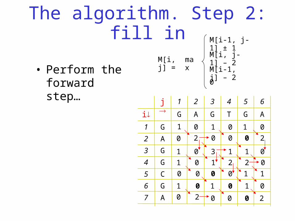
The algorithm. Step 2: fill in
• Perform the forward step…
M[i, j] =M[i, j-1] – 2M[i-1, j] – 2
M[i-1, j-1] ± 1
max
654321j
7
6
5
4
3
2
1
i
A
G
C
G
G
A
1G
AGTGAG
0
0 01 1
1
1
0
0
2 0 0 0 2
0 3 1 1 0
0 1 2
The algorithm. Step 2: fill in
• Perform the forward step…
M[i, j] =M[i, j-1] – 2M[i-1, j] – 2
M[i-1, j-1] ± 1
max
654321j
7
6
5
4
3
2
1
i
A
G
C
G
G
A
1G
AGTGAG
0
0
0 01 1
1
1
1
0
0
2 0 0 0 2
0 3 1 1 0
0 1 2 2 0
0 0 0 1 1
0 1 0 1 0
0 2 0 0 0 2

The algorithm. Step 2: fill in
• We’re done
• Find the highest cell anywhere in the matrix
M[i, j] =M[i, j-1] – 2M[i-1, j] – 2
M[i-1, j-1] ± 1
max
654321j
7
6
5
4
3
2
1
i
A
G
C
G
G
A
1G
AGTGAG
0
0
0 01 1
1
1
1
0
0
2 0 0 0 2
0 3 1 1 0
0 1 2 2 0
0 0 0 1 1
0 1 0 1 0
0 2 0 0 0 2

The algorithm. Step 3: trace back• Reconstruct path
leading to highest scoring cell
• Trace back until zero: alignment path can begin and terminate anywhere in matrix
• Alignment: GAG
GAG
M[i, j] =M[i, j-1] – 2M[i-1, j] – 2
M[i-1, j-1] ± 1
max
654321j
7
6
5
4
3
2
1
i
A
G
C
G
G
A
1G
AGTGAG
0
0
0 01 1
1
1
1
0
0
2 0 0 0 2
0 3 1 1 0
0 1 2 2 0
0 0 0 1 1
0 1 0 1 0
0 2 0 0 0 2

Local dynamic programmingMatch/mismatch = 1/-1, Gap =2
A T G A C G T
0 0 0 0 0 0 0 0
T 0 0 1 0 0 0 0 1
A 0 1 0 0 1 0 0 0
G 0 0 0 1 0 0 1 0
A 0 1 0 0 2 0 0 0
C 0 0 0 0 0 3 1 0
T 0 0 1 0 0 0 2 2
Fill the matrix (forward pass), then do trace back from highest cell anywhere in the matrix till you reach 0 or the beginning of a sequence
GACGAC

Local dynamic programming (Smith & Waterman, 1981)
i-1
j-1
Si,j = Max
Si,j + Max{S0<x<i-1,j-1 - Pi - (i-x-1)Px}
Si,j + Si-1,j-1
Si,j + Max {Si-1,0<y<j-1 - Pi - (j-y-1)Px}
0
Gap opening penalty
Gap extension penalty
This is the general DP algorithm, which is suitable for linear, affine and concave penalties, although for the example here affine penalties are used

Local dynamic programming

Global or Local Pairwise alignment
Local
Global
A B
A
B
A B
B A
AB
Local
Global
A BA
CC
A B C
A B C
A B
A
C
C

Globin fold proteinmyoglobinPDB: 1MBN
Alpha-helices are labelled ‘A’ (blue) to ‘H’ (red). The D helix can be missing in some globins:
What happens with the alignment if D-helix containing globin sequences are aligned with ‘D-less’ ones?

sandwich proteinimmunoglobulinPDB: 7FAB
Immunoglobulinstructures have variable regions where numbers of amino acids can vary substantially

TIM barrel / proteinTriosephosphate IsoMerasePDB: 1TIM
The evolutionary history of this protein family has been the subject of rigorous debate. Arguments have been made in favor of both convergent and divergent evolution. Because of the general lack of sequence homology, the ancestry of this molecule is still a mystery.

What does all this mean for alignments?
• Alignments need to be able to skip secondary structural elements to complete domains (i.e. putting gaps opposite these motifs in the shorter sequence).
• Depending on gap penalties chosen, the algorithm might have difficulty with making such long gaps (for example when using high affine gap penalties), resulting in incorrect alignment.
• Alignments are only meaningful for homologous sequences (with a common ancestor)

There are three kinds of pairwise alignments
Global alignment – align all residues in both sequences; all gaps are penalised
Semi-global alignment – align all residues in both sequences; end gaps are not penalised (zero end gap penalties)
Local alignment – align one part of each sequence; end gaps are not applicable

Easy global DP recipe for using affine gap penalties (after Gotoh)
M[i,j] is optimal alignment (highest scoring alignment until [i, j]) At each cell [i, j] in search matrix, check Max coming from:
any cell in preceding row until j-2: add score for cell[i, j] minus appropriate gap penalties;
any cell in preceding column until i-2: add score for cell[i, j] minus appropriate gap penalties;
or cell[i-1, j-1]: add score for cell[i, j] Select highest scoring cell in bottom row and rightmost column and do
trace-back
i-1
j-1Penalty = Pi + gap_length*Pe
Si,j = si,j + Max
Max{S0<x<i-1, j-1 - Pi - (i-x-1)Px}
Si-1,j-1
Max{Si-1, 0<y<j-1 - Pi - (j-y-1)Px}

Let’s do an example: global alignment
Gotoh’s DP algorithm with affine gap penalties (PAM250, Pi=10, Pe=2)
Row and column ‘0’ are filled with 0, -12, -14, -16, … if global alignment is used (for N-terminal end-gaps); also extra row and column at the end to calculate the score including C-terminal end-gap penalties. Note that only ‘non-diagonal’ arrows are indicated for clarity (no arrow means that you go back to earlier diagonal cell).
D W V T A L K
T 0 -5 0 3 1 1 0
D 4 -7 -2 0 0 -4 0
W -7 17 -6 -5 -6 -2 -3
V -2 -6 4 0 0 2 -2
L -4 -2 2 1 -2 6 -3
K 0 -3 -2 0 -1 -3 5
D W V T A L K
0 -12 -14 -16 -18 -20 -22 -24
T -12 0 -17 -14 -13 -17 -19 -22 -22
D -14 -8 -7 -14 -14 -13 -42
W -16 -21 9 -13 -19 -18
V -18 -18 -20 13 -3 -16
L -20 -22 -18 -1 14 -1 -14
K -22 -20 -21 -12
-24 -42 -41 -18 -16 -14 -12 0PAM250
Cell (D2, T4) can alternatively come from two cells (same score): ‘high-road’ or ‘low-road’

Let’s do another example: semi-global alignmentGotoh’s DP algorithm with affine gap penalties
(PAM250, Pi=10, Pe=2)
Starting row and column ‘0’, and extra column at right or extra row at bottom is not necessary when using semi global alignment (zero end-gaps). Rest works as under global alignment.
D W V T A L K
T 0 -5 0 3 1 1 0
D 4 -7 -2 0 0 -4 0
W -7 17 -6 -5 -6 -2 -3
V -2 -6 4 0 0 2 -2
L -4 -2 2 1 -2 6 -3
K 0 -3 -2 0 -1 -3 5
D W V T A L K
T 0 -5 0 3
D 4 -7 -7
W -7 21 -13
V -2 -13 25 9
L
K
PAM250

Easy local DP recipe for using affine gap penalties (after Gotoh)
M[i,j] is optimal alignment (highest scoring alignment until [i, j]) At each cell [i, j] in search matrix, check Max coming from:
any cell in preceding row until j-2: add score for cell[i, j] minus appropriate gap penalties;
any cell in preceding column until i-2: add score for cell[i, j] minus appropriate gap penalties;
cell[i-1, j-1]: add score for cell[i, j] or 0
Select highest scoring cell anywhere in matrix and do trace-back until zero-valued cell or start of sequence(s)
i-1
j-1Penalty = Pi + gap_length*Pe
Si,j = Max
Si,j + Max{S0<x<i-1,j-1 - Pi - (i-x-1)Px}
Si,j + Si-1,j-1
Si,j + Max {Si-1,0<y<j-1 - Pi - (j-y-1)Px}
0

Let’s do yet another example: local alignment
Gotoh’s DP algorithm with affine gap penalties (PAM250, Pi=10, Pe=2)
Extra start/end columns/rows not necessary (no end-gaps). Each negative scoring cell is set to zero. Highest scoring cell may be found anywhere in search matrix after calculating it. Trace highest scoring cell back to first cell with zero value (or the beginning of one or both sequences)
D W V T A L K
T 0 -5 0 3 1 1 0
D 4 -7 -2 0 0 -4 0
W -7 17 -6 -5 -6 -2 -3
V -2 -6 4 0 0 2 -2
L -4 -2 2 1 -2 6 -3
K 0 -3 -2 0 -1 -3 5
D W V T A L K
T 0 0 0 3
D 4 0 0 0
W 0 21 0 0
V 0 0 25 9
L 0 0 11
K 0 0
PAM250

Dot plots
• Way of representing (visualising) sequence similarity without doing dynamic programming (DP)
• Make search matrix as for DP, but locally represent sequence similarity by averaging using a sliding window

Dot-plots
Dot plots are calculated using a diagonal window of preset length that is slid through the search matrix --typically the central cell holds the window score (e.g. sum, average)

Dot-plotsa simple way to visualise
sequence similarity
Can be a bit messy, though...Filter: 6/10 residues have to match...

Dot-plots, what about...
• Insertions/deletions -- DNA and proteins
• Duplications (e.g. tandem repeats) – DNA and proteins
• Inversions -- DNA Dot plots are calculated using a diagonal window of preset length that is slid through the search matrix --typically the central cell holds the window score (e.g. sum, average)

Dot-plots, self-comparison
Direct repeatDirect repeat
Tandem repeatTandem repeat
Inverted repeatInverted repeat

• a heuristic– Heuristics: A rule of thumb that often helps in
solving a certain class of problems, but makes no guarantees.Perkins, DN (1981) The Mind's Best Work

For your first exam D1:Make sure you understand and can carry out
1. the ‘simple’ DP algorithm for global, semi-global and local alignment (using linear gap penalties but make sure you know the extension of the basic algorithm for affine gap penalties) and
2. The general DP algorithm for global, semi-global and local alignment (using linear, affine and concave gap penalties)!


