Contents lists available at SciVerse ScienceDirect

Journal of Economic Dynamics & Control

Journal of Economic Dynamics & Control 37 (2013) 1–17

0165-18

http://d

$ The

or the F

comme

at Irvinn Corr

E-m1 Th

Maskin

journal homepage: www.elsevier.com/locate/jedc

Pairwise trade, asset prices, and monetary policy$

Ed Nosal a,n, Guillaume Rocheteau b

a Federal Reserve Bank of Chicago, 230 S LaSalle St, Chicago, IL 60604, USAb University of California, Irvine and Federal Reserve Bank of Cleveland, USA

a r t i c l e i n f o

Article history:

Received 12 January 2011

Received in revised form

7 November 2011

Accepted 1 June 2012Available online 16 July 2012

JEL classification:

E40

E50

Keywords:

Search

Money

Bilateral trades

Inflation

Asset prices

89/$ - see front matter & 2012 Elsevier B.V. A

x.doi.org/10.1016/j.jedc.2012.07.005

views expressed are those of the authors and

ederal Reserve System. We thank Veronica G

nts, and seminar participants at the Bank of C

e, and the 2008 annual meeting of the Societ

esponding author. Tel.: þ1 312 322 6070; fa

ail address: ed.nosal@chi.frb.org (E. Nosal).

e recognizability of money is an old theme i

(1996).

a b s t r a c t

We construct a search-theoretic model where fiat money coexists with real assets, and

all assets can be used as a media of exchange. The terms of trade in bilateral matches

are determined by a pairwise Pareto-efficient pricing mechanism. We do not have to

appeal to exogenous liquidity constraints to generate asset prices that are consistent

with the following facts: (i) fiat money can be valued despite being dominated in its

rate of return; (ii) real assets with identical dividend flows can have different rates of

return; and (iii) an increase in inflation raises asset prices, lowers their returns, and

widens the rate-of-return differences between assets. On the normative side we show

that there is a range of inflation rates that implement the first-best allocation.

& 2012 Elsevier B.V. All rights reserved.

1. Introduction

What determines an asset’s liquidity? More than 20 years ago, Kiyotaki and Wright (1989) provided an answer in thecontext of a monetary model with bilateral exchange. They found that the moneyness of an asset depends on its physicalproperties (e.g., storage costs), the fundamentals of the economy (e.g., the pattern of specialization) and conventions (e.g., howagents coordinate on one of many possible equilibria). These insights were derived under the extreme portfolio restriction thatagents cannot hold more than one unit of an asset, and the stark assumption that assets and goods are indivisible.Subsequently, these restrictions and assumptions have been relaxed, see e.g., Shi (1997) and Lagos and Wright (2005), whichled to a renewed interest in the question that prompted this literature in the first place: What makes money money?

Recent work has shown that liquidity differences across assets can arise from either informational asymmetries orexogenous asset specific liquidity constraints. For example, Lester et al. (2012) show that fiat money is a superior means ofpayment because it is can be authenticated at zero cost.1 Rocheteau (2011) finds that when asset holders are privately

ll rights reserved.

not necessarily those of the Federal Reserve Bank of Chicago, the Federal Reserve Bank of Cleveland

uerrieri for her insightful discussion, an anonymous referee and the editor, Jim Bullard, for their

anada, Federal Reserve Bank of New York, Federal Reserve Bank of St. Louis, University of California

y of Economic Dynamics.

x: þ1 312 322 5943.

n monetary theory. Recent formalizations include Williamson and Wright (1994) and Banarjee and

E. Nosal, G. Rocheteau / Journal of Economic Dynamics & Control 37 (2013) 1–172

informed about dividends, the liquidity of assets depends on the properties of their dividend processes. Kiyotaki andMoore (2005) and Lagos (2010) impose exogenous liquidity constraints on some financial transactions in order to matchsome asset pricing facts that are viewed as anomalies.

In this paper, we take an alternative approach to generate liquidity differences across assets that does not require eitherinformational asymmetries or exogenous constraints on payments. We generalize the argument of Zhu and Wallace(2007), who propose a trading mechanism for bilateral matches that has good normative properties and that, from atransactions perspective, treats assets asymmetrically.2 The allocations for our bilateral trading mechanism, like Zhu andWallace (2007), are Pareto efficient.3 We further restrict our trading mechanism by requiring asset pricing patterns to bethe same those from models with exogenous liquidity constraints. In particular, asset prices should exhibit: (i) rate ofreturn dominance; (ii) rate of return differences between assets with identical cash flows; (iii) and a positive correlationbetween asset prices and inflation. The key difference in our approach relative to that of Kiyotaki and Moore (2005) andLagos (2010) is that all assets held by an agent can be used to finance consumption opportunities without any restrictions.Our mechanism does not leave any asset unused as a means of payment, unless there are no further gains from trade.4 Thekey difference in our approach relative to that of Zhu and Wallace (2007) is that our trading mechanism is more generalthan what they consider and, as a consequence, our model is able to deliver a non-degenerate liquidity structure of assetreturns. The family of trading mechanisms that we consider is parametrized by a single parameter – just like thegeneralized Nash solution – and it admits as particular cases the pricing mechanisms considered in Geromichalos et al.(2007), Lagos (2010), Lagos and Rocheteau (2008), and Zhu and Wallace (2007).

Our trading mechanism is embedded into a search-theoretic model with divisible money, along the lines of Lagos andWright (2005), where a lack of double coincidence of wants and the absence of a record-keeping technology generate anexplicit need for a tangible medium of exchange. There are multiple types of assets: money and real assets that yield a flowof real dividends.5

The main insights of our theory are as follows. First, fiat money can be held and valued despite being dominated in itsrate of return by competing assets. In contrast to earlier works, we do not need to impose trading restrictions to generate arate of return dominance pattern: a plain-vanilla Lagos–Wright model can account for this puzzle. Second, the model iscapable of generating a liquidity-based structure of asset yields, where assets can exhibit different rates of returns, even ifthey share the same risk characteristics, or if agents are risk-neutral.6 Those rate of return differences, which are allanomalies from the standpoint of standard asset pricing theories, reflect differences in the liquidity of the assets; someassets can be liquidated at better terms of trade than others. Third, our model also has implications for the transmissionmechanism of monetary policy to asset prices. Under our pricing protocol, real assets have a liquidity value in the sensethat a buyer is able to capture some surplus in a bilateral meeting when paying with real assets. Hence, an increase ininflation will raise their prices and lowers their returns. Moreover, inflation widens the rate of return differences betweenassets. And finally, from a normative standpoint, there is a range of inflation rates that implement the first-best allocation,including the Friedman rule. As a consequence, a small inflation above the Friedman rule does not impose a welfare cost onsociety.

2. The environment

Time is discrete and continues forever. The economy is populated with a [0,1] continuum of infinitely lived agents. As inLagos and Wright (2005), each period is divided into two subperiods, called DM and CM. In the first subperiod, DM, tradetakes place in decentralized markets, where agents are bilaterally matched in a random fashion. In the second subperiod,CM, trade takes place in competitive markets.

2 One can interpret bilateral meetings as an over-the-counter market. Formalizations of over-the-counter markets in finance have been proposed by

Duffie, Garleanu, and Pedersen (2005), Weill (2008), and Lagos and Rocheteau (2008).3 Shi (1997) and Lagos and Wright (2005) assume that the terms of trade in bilateral matches are determined by the generalized Nash bargaining

solution. Aruoba et al. (2007) investigate the robustness of the results to alternative bargaining solutions. Other mechanisms have been studied such as

auctions and competitive posting. For a mechanism design approach, where the mechanism is chosen by normative considerations, see Hu et al. (2009).4 More generally, our paper is related to the recent literature in macroeconomics that takes into account the transaction role of assets in order to

explain asset pricing anomalies and the effects of monetary policy on assets’ returns. For instance, Bansal and Coleman (1996) explain the risk-free rate

and the equity premium puzzles in a pure exchange economy where there are different transaction costs associated with the use of different means of

payment, e.g., fiat money, government bonds and credit. Recently, Aruoba and Schorfheide (2010) estimated a search-based monetary DSGE model in

which agents in the decentralized market can only use a fraction of their capital stock holdings in addition to money to finance consumption

opportunities. They find that the estimated fraction of capital that is liquid is close to zero.5 The first attempt to introduce capital goods into the Lagos–Wright model is Aruoba and Wright (2003), but capital goods were not allowed to be

used as means of payment in bilateral matches. Lagos and Rocheteau (2008) relax the restriction on the use of capital as a means of payment, and show

that fiat money and capital can coexist provided that there is a shortage of capital to be used as means of payment. In a similar context Rocheteau (2011)

adopts a mechanism design approach to show that the coexistence of money and higher-return assets is both socially optimal and individually rational.

Geromichalos et al. (2007) follow a similar approach but assume that capital is in fixed supply. Lagos (2010) calibrates the model where money is

replaced by risk-free bonds and capital is a risky asset, and shows that it can account for the risk-free rate and equity premium puzzles under a mild

restriction on the use of capital as means of payments.6 Wallace (2000) provides a theory of the liquidity structure of asset yields based on the indivisibility of assets. Weill (2008) explains differences in

liquidity across seemingly identical assets by the presence of thick market externalities in decentralized asset markets.

E. Nosal, G. Rocheteau / Journal of Economic Dynamics & Control 37 (2013) 1–17 3

In the DM, agents produce and consume perishable goods that come in different varieties. The probability that an agentis matched with someone who produces a good he wishes to consume is ar1=2. Symmetrically, the probability that anagent meets someone who consumes the good he produces is ar1=2. For convenience, and without loss of generality, werule out double-coincidence-of-wants meetings. In the CM, all agents are able to consume and produce a perishable good.7

An agent’s utility function is

EX1t ¼ 0

bt½uðyb

t Þ�cðyst Þþxt�ht �

" #,

where yb is consumption and ys is production of the DM good, x is consumption of the CM good, h is hours of work toproduce the CM good, and b¼ ð1þrÞ�1

2 ð0,1Þ is the discount factor across periods. We assume that uðyÞ�cðyÞ iscontinuously differentiable, strictly increasing and concave. In addition, cð0Þ ¼ uð0Þ ¼ 0, u0ð0Þ ¼ þ1 , u0ðþ1Þ¼ 0, andthere exists a ynoþ1 such that u0ðynÞ ¼ c0ðynÞ. The technology to produce the CM good is linear and one-to-one in hours,i.e., h hours of work produce h units of the CM good.8

Agents cannot commit, and their trading histories are private information. This implies that credit arrangements areinfeasible. The infeasibility of credit, in conjunction with the specialization of agents’ consumption and production in theDM, generates a role for a medium of exchange. There are two storable and perfectly divisible assets in the economy. Bothcan serve as media of exchange.9 There is a real asset that is in fixed supply, A40. In each CM subperiod, one unit of thereal asset generates a dividend equal to k40 units of the CM good. There also exists an intrinsically useless asset calledfiat money. The quantity of money at the beginning of period t is denoted Mt. The money supply grows at the gross rateg4b, where g�Mtþ1=Mt , via lump-sum transfers or taxes in the CM.10 In the DM, producers and consumers in a bilateralmatch can exchange the assets for one other or for the consumption good. In the CM, assets are traded with the generalgood in competitive markets.

The asset prices at date t are measured in terms of the date t CM good. The price of money is denoted by ft and theprice of the real asset is denoted by qt. We will focus our attention on stationary equilibria, where ftMt and qt are constant.

3. Pricing

In this section, we describe the determination of the terms of trade in bilateral meetings in the DM. Before we do this,however, it will be useful to show some properties of an agent’s value function in the CM, W, since it tells us how agentsvalue the assets they give up or receive in the DM. The value function of an agent entering the CM holding a portfolio of a

units of real asset and z units of real balances is

Wða,zÞ ¼ maxx,h,a0 ,z0

fx�hþbVða0,z0Þg ð1Þ

s:t: gz0 þqa0 þx¼ zþhþaðqþkÞþT , ð2Þ

where T �ftðMtþ1�MtÞ, measured in terms of the CM good, is the lump-sum transfer associated with a money injection.At the start of the CM, each unit of the real asset generates k units of the CM good. Then assets can be bought or sold in acompetitive market at the price q. The agent chooses his net consumption, x�h, and the portfolio, ða0,z0Þ, that he brings intothe subsequent DM. Each unit of real balances acquired in the CM of date t will turn into ftþ1=ft ¼ g�1 units of realbalances in date tþ1. So, in order to have z0 units of real balances in the next period, an agent must acquire gz0 units in thecurrent period.

Substituting x�h from (2) into (1) gives

Wða,zÞ ¼ zþaðqþkÞþTþ maxa0 ,z0f�gz0�qa0 þbVða0,z0Þg: ð3Þ

From (3), the CM value function is linear in the agent’s wealth: this property will prove especially convenient in terms ofsimplifying the pricing problem in the DM. Note also that the choice of the agent’s new portfolio, ða0,z0Þ, is independent ofthe portfolio that he brought into the CM subperiod, (a,z), as a consequence of quasi-linear preferences.

Consider now a match in the DM between a buyer holding portfolio (a,z) and a seller holding portfolio ðas,zsÞ. The termsof trade are given by the output yZ0 produced by the seller and the transfer of assets ðtm,taÞ 2 ½�zs,z� � ½�as,a� from thebuyer to the seller, where tm is the transfer of real balances and ta is the transfer of real assets. (If the transfer is negative,

7 We could assume that the same goods which are traded in the DM are also traded in the CM. However, the specialization in terms of preferences

and technologies is irrelevant in the complete information, competitive CM subperiod.8 Following Lagos and Wright (2005), we could adopt a more general utility function for the CM, UðxÞ�h with U00o0. Our results would not be

affected provided that the nonnegativity constraint for the number of hours, hZ0, is not binding in equilibrium.9 The literal interpretation in the model is that assets are used as money. An equivalent interpretation would be to assume that assets serve as

collateral to secure loans to be repaid in the CM subperiod.10 If go1 the government can force agents to pay taxes in the CM. In a related model, Andolfatto (2010) considers the case where the government

has limited coercion power – it cannot confiscate output and cannot force agents to work – and the payment of lump-sum taxes is voluntary. Here, agents

can avoid paying taxes by not accumulating money balances. He shows that if agents are sufficiently impatient, then the Friedman rule is not incentive-

feasible, i.e., there is an induced lower bound on deflation. See also Hu et al. (2009).

E. Nosal, G. Rocheteau / Journal of Economic Dynamics & Control 37 (2013) 1–174

then the seller is delivering assets to the buyer.) The procedure that determines the terms of trade in the DM generalizesthe one suggested by Zhu and Wallace (2007).11 The procedure has two steps. The first step generates a payoff or surplusfor the buyer, denoted as U

b, which is equal to what he would obtain in a bargaining game if he had all the bargaining

power, but was facing a liquidity constraint. Specifically, in this ‘‘virtual game’’ it is assumed that the buyer can transfer atmost all his real balances and a fraction y of his real asset holdings, i.e., tzrz and tarya.12 (Zhu and Wallace (2007)assume that y¼ 0; Lagos and Rocheteau (2008) and Geromichalos et al. (2007) assume y¼ 1.) The liquidity constraint onreal asset holdings in the virtual game is chosen purposely to be reminiscent to the one used in Kiyotaki and Moore (2005),where individuals can only use a fraction of their capital goods to finance investment opportunities.13 From the buyer’sstandpoint, it is as if he was trading in the Kiyotaki–Moore economy. The liquidity constraint is also reminiscent of theconstraint in Lagos (2010), where y¼ 0 in a fraction of the matches and y¼ 1 in the remaining matches. Note that theoutput and wealth transfers in the first step are virtual in the sense that they are simply used to determine the buyer’ssurplus, U

b. The actual output and wealth transfer are determined in the second step so as to generate a pairwise Pareto-

efficient trade. In the second step, the actual trade maximizes the seller’s surplus subject to the constraint that the buyerreceives a surplus at least equal to U

b. The only restrictions placed on the transfer of either asset is that an agent cannot

transfer more than he has, i.e., �asrtara and �zsrtmrz.The first step of our pricing protocol, which determines the buyer’s surplus U

b, solves the following problem:

Ubða,zÞ ¼ max

y,tm ,ta

½uðyÞþWða�ta,z�tzÞ�Wða,zÞ�

s:t: �cðyÞþWðasþta,zsþtmÞZWðas,zsÞ

tm 2 ½�zs,z�, ta 2 ½�as,ya�:

The buyer in this virtual game maximizes his surplus, subject to the participation constraint of the seller and theconstraints on the transfer of his asset holdings: the buyer can transfer all his money balances but only hand over afraction y of his real asset.14 Using the linearity of Wða,zÞ, the above problem can be rewritten as

Ubða,zÞ ¼ max

y,tm ,ta

½uðyÞ�tm�taðqþkÞ� ð4Þ

s:t:�cðyÞþtmþtaðqþkÞZ0 ð5Þ

�zs�asðqþkÞrtmþtaðqþkÞrzþyaðqþkÞ: ð6Þ

From this formulation, note that what matters is the total value of the transfer of assets, tmþtaðqþkÞ, and not itscomposition in terms of money and real asset. Moreover, from the seller’s participation constraint, yZ0 requirestmþtaðqþkÞZ0. Thus, the constraint that the seller cannot transfer more than his wealth is irrelevant, and the buyer’spayoff is independent of ðas,zsÞ.15 From this, it is easy to see that the buyer’s payoff is a function of only his ‘‘liquid’’wealth, zþyaðqþkÞ, the wealth he can use in the first step of the virtual game to maximize his payoff.

We now describe some of the properties of buyer’s surplus function, Ubða,zÞ.

Lemma 1. The buyer’s payoff is uniquely determined and satisfies

Ubða,zÞ ¼

uðynÞ�cðynÞ if zþyaðqþkÞZcðynÞ,

u3c�1½zþyaðqþkÞ��z�yaðqþkÞ otherwise,

(ð7Þ

where yn ¼ arg maxy½uðyÞ�cðyÞ�. If zþyaðqþkÞocðynÞ, then Ubða,zÞ is strictly increasing and strictly concave with respect to

each of its arguments. Moreover, Ubða,zÞ is jointly concave (but not strictly) with respect to (a,z).

Proof. The solution to (4)–(6) is y¼ yn and Ub¼ uðynÞ�cðynÞ iff zþyaðqþkÞZcðynÞ; otherwise, y¼ c�1½zþyaðqþkÞ� and

ðtm,taÞ ¼ ðz,yaÞ.

11 This trading mechanism is not a strategic game. The main objective of the paper is to show that there exists Pareto-efficient trading mechanisms

that generate liquidity and rate-of-return differences across assets. Nevertheless, later in this section and in the Appendix, we propose a simple two-stage

strategic game that provides foundations for our trading mechanism.12 We do not constrain the transfer of asset holdings of the seller, but this is without loss in generality. Indeed, it is easy to check that if ta Z�yas in

the first step of the trading protocol, the buyer’s payoff is unaffected.13 Kiyotaki and Moore (2005) consider an economy with two assets, capital and land. Land is in fixed supply while capital is accumulated. Both assets

are inputs in the production of the final good. Individuals receive random opportunities to invest. In order to finance investment, they can use all their

land – land is ‘‘completely liquid’’ – but only a fraction y of their capital holdings. So land is analogous to money in our formulation, while capital is

similar to our real asset.14 In principle, U

bshould also have zs and as as arguments. Here we anticipate on the result according to which the terms of trade in this virtual game

are independent of the seller’s portfolio.15 Indeed, from the seller’s participation constraint, (5), yZ0 implies tmþtaðqþkÞZ0. Therefore, the inequality, �zs�asðqþkÞrtmþtaðqþkÞ, in (6)

is never binding.

E. Nosal, G. Rocheteau / Journal of Economic Dynamics & Control 37 (2013) 1–17 5

If zþyaðqþkÞocðynÞ, then

Ub

a ¼@U

b

@a¼ yðqþkÞ u0ðoÞ

c0ðoÞ�1

� �40, ð8Þ

Ub

z ¼@U

b

@z¼

u0ðoÞc0ðoÞ

�140, ð9Þ

where o¼ c�1½zþyaðqþkÞ�; Ubða,zÞ is increasing with respect to each of its arguments. As well

Ub

zz ¼u00ðoÞc0ðoÞ�u0ðoÞc00ðoÞ

½c0ðoÞ�3o0,

Ub

za ¼ yðqþkÞ u00ðoÞc0ðoÞ�u0ðoÞc00ðoÞ½c0ðoÞ�3

� �o0,

Ub

aa ¼ ½yðqþkÞ�2 u00ðoÞc0ðoÞ�u0ðoÞc00ðoÞ

½c0ðoÞ�3

� �o0,

Ubða,zÞ is strictly concave with respect to each of its arguments and U

b

aaUb

zz�ðUb

zaÞ2¼ 0. Hence, U

bða,zÞ is jointly concave,

but not strictly jointly concave. &

The second step of the pricing protocol determines the seller’s surplus, Usða,zÞ, and the actual terms of trade, ðy,tm,taÞ,

as functions of the buyer’s portfolio in the match, (a,z). By construction, the terms of trade are chosen so that the allocationis pairwise Pareto-efficient. The allocation solves the following problem:

Usða,zÞ ¼ max

y,tm ,ta

½�cðyÞþtmþtaðqþkÞ� ð10Þ

s:t: uðyÞ�tm�taðqþkÞZUbða,zÞ ð11Þ

�zsrtmrz, �asrtara, ð12Þ

Notice that in this problem, the use of the real asset as means of payment is not restricted. Moreover, Usða,zÞZ0 since the

allocation determined in the first step of the pricing procedure is still feasible in the second step and, from the seller’sparticipation constraint, (5), his surplus is nonnegative. It is straightforward to characterize the solution to the second-stepproblem (10)–(12).

Lemma 2. If zþaðqþkÞZuðynÞ�Ubða,zÞ, then the terms of trade in bilateral meetings satisfy

y¼ yn, ð13Þ

tmþtaðqþkÞ ¼ uðynÞ�Ubða,zÞ, ð14Þ

otherwise

y¼ u�1½zþaðqþkÞþUbða,zÞ�, ð15Þ

ðta,tmÞ ¼ ða,zÞ: ð16Þ

The seller’s payoff and output are uniquely determined. The composition of the payment between money and the realasset is unique if the output is strictly less than the efficient level, yn. If zþaðqþkÞ4uðynÞ�U

bða,zÞ, then there are a

continuum of transfers ðta,tmÞ that achieve (14).Consider the case where zþaðqþkÞouðynÞ�U

bða,zÞ, i.e., the output depends on the composition of the buyer’s portfolio.

From (15) and (16) one can compute the quantity of output a buyer can acquire with an additional unit of wealth. If anagent accumulates an additional unit of real balances, his consumption in the DM increases by

@y

@z¼

u0ðoÞc0ðoÞu0ðyÞ ,

where o¼ c�1½zþyaðqþkÞ�. If the agent accumulates an additional unit of the real asset, which promises qþk units ofoutput in the next CM, then

ðqþkÞ�1 @y

@a¼

1þyu0ðoÞc0ðoÞ

�1

� �u0ðyÞ

:

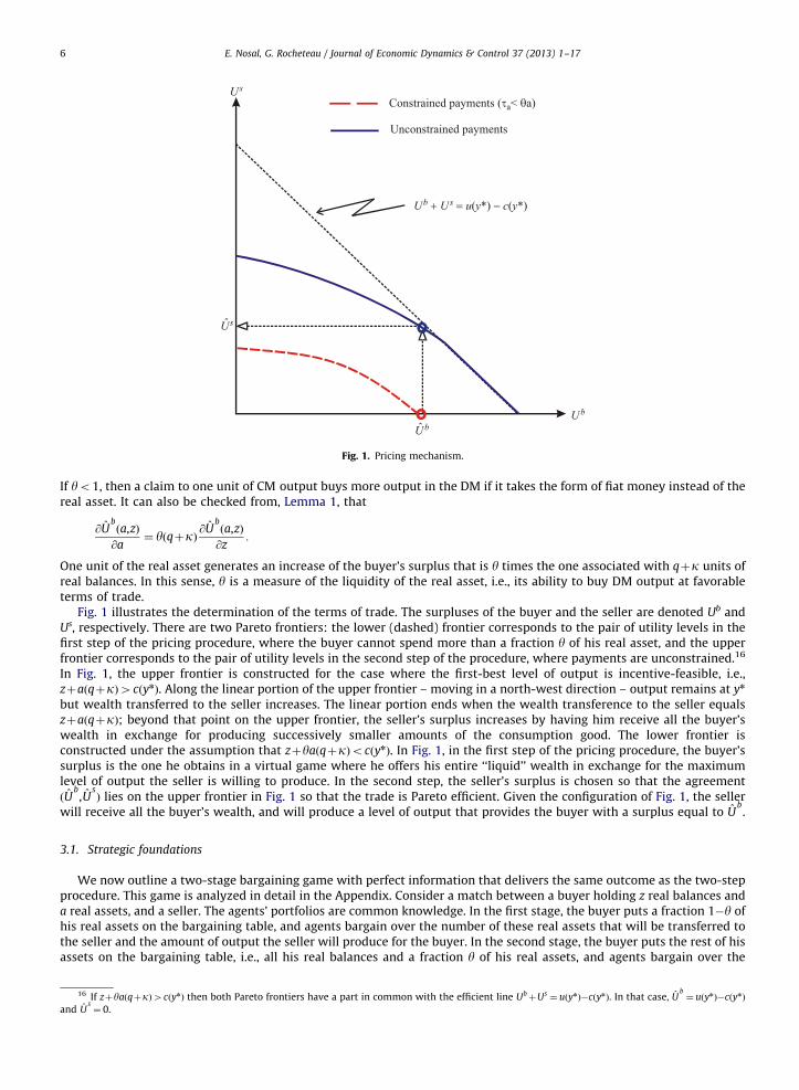
Constrained payments (τa< θa)

Unconstrained payments

Ub + Us = u(y*) − c(y*)

Us

Ub

Ubˆ

Usˆ

Fig. 1. Pricing mechanism.

E. Nosal, G. Rocheteau / Journal of Economic Dynamics & Control 37 (2013) 1–176

If yo1, then a claim to one unit of CM output buys more output in the DM if it takes the form of fiat money instead of thereal asset. It can also be checked from, Lemma 1, that

@Ubða,zÞ

@a¼ yðqþkÞ @U

bða,zÞ

@z:

One unit of the real asset generates an increase of the buyer’s surplus that is y times the one associated with qþk units ofreal balances. In this sense, y is a measure of the liquidity of the real asset, i.e., its ability to buy DM output at favorableterms of trade.

Fig. 1 illustrates the determination of the terms of trade. The surpluses of the buyer and the seller are denoted Ub andUs, respectively. There are two Pareto frontiers: the lower (dashed) frontier corresponds to the pair of utility levels in thefirst step of the pricing procedure, where the buyer cannot spend more than a fraction y of his real asset, and the upperfrontier corresponds to the pair of utility levels in the second step of the procedure, where payments are unconstrained.16

In Fig. 1, the upper frontier is constructed for the case where the first-best level of output is incentive-feasible, i.e.,zþaðqþkÞ4cðynÞ. Along the linear portion of the upper frontier – moving in a north-west direction – output remains at yn

but wealth transferred to the seller increases. The linear portion ends when the wealth transference to the seller equalszþaðqþkÞ; beyond that point on the upper frontier, the seller’s surplus increases by having him receive all the buyer’swealth in exchange for producing successively smaller amounts of the consumption good. The lower frontier isconstructed under the assumption that zþyaðqþkÞocðynÞ. In Fig. 1, in the first step of the pricing procedure, the buyer’ssurplus is the one he obtains in a virtual game where he offers his entire ‘‘liquid’’ wealth in exchange for the maximumlevel of output the seller is willing to produce. In the second step, the seller’s surplus is chosen so that the agreementðU

b,U

sÞ lies on the upper frontier in Fig. 1 so that the trade is Pareto efficient. Given the configuration of Fig. 1, the seller

will receive all the buyer’s wealth, and will produce a level of output that provides the buyer with a surplus equal to Ub.

3.1. Strategic foundations

We now outline a two-stage bargaining game with perfect information that delivers the same outcome as the two-stepprocedure. This game is analyzed in detail in the Appendix. Consider a match between a buyer holding z real balances anda real assets, and a seller. The agents’ portfolios are common knowledge. In the first stage, the buyer puts a fraction 1�y ofhis real assets on the bargaining table, and agents bargain over the number of these real assets that will be transferred tothe seller and the amount of output the seller will produce for the buyer. In the second stage, the buyer puts the rest of hisassets on the bargaining table, i.e., all his real balances and a fraction y of his real assets, and agents bargain over the

16 If zþya qþkð Þ4cðynÞ then both Pareto frontiers have a part in common with the efficient line UbþUs¼ uðynÞ�cðynÞ. In that case, U

b¼ uðynÞ�cðynÞ

and Us¼ 0.

E. Nosal, G. Rocheteau / Journal of Economic Dynamics & Control 37 (2013) 1–17 7

transfer of assets to the seller and the amount of output the seller produces.17 The fraction 1�y of the buyer’s real assetsthat are on the negotiation table in the first stage cannot be used in the second-stage negotiation. For example, if the firststage results in no output being produced and no real assets being exchanged, then, even though the buyer has a realassets going into the second stage, he can only use the ya of them at that time.

The game that agents play is as follows. In the first stage the seller makes an offer ðy1,t1aÞ, where y1 2 Rþ is output the

seller will produce and t1a 2 ½0,ð1�yÞa� is the amount of real assets the buyer must transfer to the seller. The buyer accepts

or rejects the offer. If the offer is accepted, then the production/consumption of the good and the transfer of real assets takeplace. In the second stage the buyer makes an offer ðy2,t2

a ,t2mÞ, where y2 2 Rþ is output, t2

mr ½0,z� is a transfer of realbalances and t2

a 2 ½0,ya� is a transfer of real assets. The seller accepts or rejects the offer. If the offer is accepted, theproduction/consumption of the good and the transfer of real balances and assets take place.

4. Equilibrium

We incorporate the pricing mechanism, described in Section 3, in our general equilibrium model. Let yða,zÞ, taða,zÞ andtmða,zÞ represent the output and transfer outcomes from the pricing mechanism when the buyer in the match has portfolioða,zÞ. The value to an agent of holding portfolio ða,zÞ at the beginning of the DM, Vða,zÞ, is given by

Vða,zÞ ¼ afu½yða,zÞ�þW ½a�taða,zÞ,z�tmða,zÞ�gþaEf�c½yð ~a, ~zÞ�þW ½aþtað ~a, ~zÞ,zþtmð ~a, ~zÞ�gþð1�2aÞWða,zÞ: ð17Þ

With probability a, the agent is the buyer in a match. He consumes yða,zÞ and delivers the assets ½taða,zÞ,tmða,zÞ� to theseller.18 As established in Lemmas 1 and 2, the terms of trade ðy,ta,tmÞ only depend on the portfolio of the buyer in thematch. With probability a the agent is the seller in the match. He produces y and receives ðta,tmÞ from the buyer whereðy,ta,tmÞ is a function of the buyer’s portfolio ð ~a, ~zÞ. The expectation is taken with respect to ð ~a, ~zÞ, since the distribution ofasset holdings might be non-degenerate, assuming that the buyer partner is chosen at random from the whole populationof potential buyers. Finally, with probability 1�2a the agent is neither a buyer nor a seller. Using the linearity of Wða,zÞ andthe expressions for the buyer’s and the seller’s surpluses, (17) can be rewritten more compactly as

Vða,zÞ ¼ aUbða,zÞþaEU

sð ~a, ~zÞþWða,zÞ: ð18Þ

If the agent was living in an economy with exogenous liquidity constraints where he can only transfer a fraction y of his real assetholdings, as in Kiyotaki and Moore (2005) or Lagos (2010), then the main difference would be that EU

sð ~a, ~zÞ ¼ 0 (assuming that

the buyer makes take-it-or-leave-it-offers). Consequently, an agent’s choice of portfolios in both economies would be similar.Substituting Vða,zÞ, as given by (18), into (3), and simplifying, an agent’s portfolio solves

ða,zÞ 2 arg maxa,zf�gz�qaþb½aU

bða,zÞþzþaðqþkÞ�g: ð19Þ

The portfolio is chosen so as to maximize the expected discounted utility of the agent if he happens to be a buyer in thenext DM minus the effective cost of the portfolio. The cost of holding an asset is its purchase price minus its discountedresale price plus its dividend. Rearranging (19), it simplifies further to

ða,zÞ 2 arg maxa,zf�iz�arðq�qnÞþaU

bða,zÞg, ð20Þ

where i� ðg�bÞ=b represents the cost of holding real balances, rðq�qnÞ is the cost of holding the real asset where qn � k=r isthe discounted sum of the real asset’s dividends. The first-order (necessary and sufficient) conditions for this (concave)problem are

�iþa u0ðoÞc0ðoÞ �1

� �þr0, ‘‘¼ ’’ if z40, ð21Þ

�rðq�qnÞþyðqþkÞa u0ðoÞc0ðoÞ �1

� �þr0, ‘‘¼ ’’ if a40, ð22Þ

where ½x�þ ¼maxðx,0Þ and o¼ c�1½zþyaðqþkÞ�. The term ½u0ðoÞ=c0ðoÞ�1�þ in (21) represents the liquidity return of realbalances, i.e., the increase in the buyer’s surplus from holding an additional unit of money. From (22), the liquidity returnof 1=ðqþkÞ units of the real asset is y times the liquidity return of real balances.

Finally, the asset price is determined by the market clearing conditionZ½0,1�

aðjÞ dj¼ A, ð23Þ

where a(j) is the asset choice of agent j 2 ½0,1�.

17 This bargaining process is related to the notion of gradual bargaining, or bargaining with an agenda, according to which the parties are to reach

agreements on several issues negotiated one after another. See, e.g., O’Neill et al. (2004). In our context, the first issue is how much output a fraction 1�yof the real assets can buy; the second issue is how much output real balances and a fraction y of the real assets can buy.

18 Recall from Lemma 2 that even though the terms of trade ðta ,tmÞmay not be uniquely determined, the transfer of wealth, tmþtaðkþqÞ, is unique.

E. Nosal, G. Rocheteau / Journal of Economic Dynamics & Control 37 (2013) 1–178

Definition 1. An equilibrium is a list f½aðjÞ,zðjÞ�j2½0,1�,½yða,zÞ,taða,zÞ,tmða,zÞ�,qg that satisfies (13)–(16), (20) and (23). Theequilibrium is monetary if

R½0,1�zðjÞdj40.

Consider first nonmonetary equilibria, where the real asset is the only means of payment in the DM. In this case, zðjÞ ¼ 0for all j.

Proposition 1. There is a nonmonetary equilibrium, and it is such that q 2 ½qn,þ1Þ:

(i)

If y¼ 0, then q¼ qn. (ii) If y40, then q is the unique solution to

qnþkqþk þ

yar

u03c�1½yAðqþkÞ�c03c�1½yAðqþkÞ�

�1

� �þ¼ 1: ð24Þ

If yAðqnþkÞZcðynÞ, then q¼ qn; otherwise q4qn.

Proof. Define the demand correspondence for the real asset as

AdðqÞ ¼

Z½0,1�

aðjÞdj : aðjÞ 2 arg maxf�arðq�qnÞþaUbða,0Þg

� �:

The market clearing condition, (23), can then be re-expressed as A 2 AdðqÞ. First, suppose y¼ 0. From (7), U

bða,0Þ ¼ 0 for all

aZ0. Then, AdðqÞ ¼ f0g for all q4qn and Ad

ðqnÞ ¼ ½0,þ1Þ. Consequently, the unique solution to A 2 AdðqÞ is q¼ qn.

Next, suppose y40. In order to characterize AdðqÞ we distinguish three cases:

1.

If q4qn then AdðqÞ ¼ fag where aocðynÞ=yðqþkÞ is the unique solution to

rðq�qnÞ ¼ aUb

aða,0Þ: ð25Þ

To see this, recall from Lemma 1 that Ubða,0Þ is strictly concave with respect to its first argument over the domain

½0,cðynÞ=yðqþkÞ�, Ub

að0,0Þ ¼1 and Ub

aða,0Þ ¼ 0 for all aZcðynÞ=yðqþkÞ. Substituting Ub

a by its expression given by (8) into

(25) and rearranging, one obtains

qnþkqþk þ

yar

u03c�1½yaðqþkÞ�c03c�1½yaðqþkÞ�

�1

� �¼ 1: ð26Þ

Note that the left-hand side is strictly decreasing in both q and a; hence, a is strictly decreasing in q. So, for all q4qn,

AdðqÞ is single-valued and strictly decreasing. Moreover, as q-qn, a-cðynÞ=ðyðqnþkÞÞ and as q-1, a-0.

b

2. If q¼ qn, then Ad

ðqnÞ ¼ argmaxaZ0fUaða,0Þg ¼ ½cðynÞ=yðqnþkÞ,þ1Þ.

3. If qoqn, then the agent’s problem has no solution.

In summary, Ad qð Þ is upper hemi-continuous over ½qn,1Þ and its range is ½0,1Þ. Hence, a solution A 2 AdðqÞ exists.

Furthermore, any selection from AdðqÞ is strictly decreasing in q 2 ½qn,1Þ, so there is a unique q such that A 2 Ad

ðqÞ. IfAZcðynÞ=ðyðqnþkÞÞ, then A 2 Ad

ðqÞ implies q¼ qn. If AocðynÞ=ðyðqnþkÞÞ, then A 2 AdðqÞ implies that q solves (26) with a¼A,

i.e., (24). &

If y¼ 0, as in Zhu and Wallace (2007), then the real asset is fully illiquid in the sense that holding the asset does notallow the buyer to extract a surplus from his trade in the DM. In this case the asset is priced at its fundamental value,q¼ qn. Since buyers are indifferent in terms of how much asset they hold, the equilibrium output is indeterminate. There isan equilibrium where buyers hold no assets (i.e., all assets are held by sellers) and there is no trade in the DM. There is alsoan equilibrium where all buyers hold A units of the asset and the output level in the DM is min½yn,c�1ðAðqnþkÞÞ�. (Thissecond equilibrium is the one that would be obtained by taking the limit as y-0.)

If y40, then the buyer can obtain a positive surplus from holding the asset in the DM. If the intrinsic value of the stockof the real asset, AðqnþkÞ, is sufficiently high, and if it is not too illiquid, i.e., y is not too low, then the buyer can extract theentire surplus of the match. An additional unit of asset does not affect the buyer’s trade surplus in the DM so that the assethas no liquidity value and its price corresponds to its fundamental price, q¼ qn ¼ k=r. The distribution of asset holdings isnot uniquely determined, but this indeterminacy is payoff irrelevant since the output traded in all matches in the DM isyn. In contrast, if the intrinsic value of the asset is low, or if the asset is very illiquid (y is low but positive), then the price ofthe asset raises above its fundamental value because it is useful to the buyer to increase his surplus in the DM. In this case,the equilibrium and the distribution of asset holdings – which is degenerate – are unique.

It is rather interesting to note from (24) that the allocation can be socially efficient, y¼ yn, even when q4qn. It can bethe case that the value of the buyer’s liquid portfolio, yaðqþkÞ, is insufficient to purchase yn in the DM – i.e., yaðqþkÞocðynÞ – but the total value of the buyer’s portfolio can be sufficient to support an output of yn, i.e., aðqþkÞZuðynÞ�U

bða,zÞ.

Let’s now turn to monetary equilibria.

E. Nosal, G. Rocheteau / Journal of Economic Dynamics & Control 37 (2013) 1–17 9

Proposition 2. There exists a monetary equilibrium iff

Aoðr�iyÞ

ykð1þrÞ‘ðiÞ, ð27Þ

where ‘ðiÞ is unique and implicitly defined by

1þi

a¼

u03c�1ð‘Þ

c03c�1ð‘Þ: ð28Þ

In a monetary equilibrium, the asset price is uniquely determined by

q¼kð1þ iyÞ

r�iyZqn: ð29Þ

Proof. With a slight abuse of notation, define Ubð‘Þ ¼ U

bða,zÞ where ‘¼ zþyaðqþkÞ. (Notice from Lemma 1 that (a,z)

matters for the buyer’s payoff only through zþyaðqþkÞ.) Then, the agent’s portfolio problem (20) can be re-expressed as

ða,‘Þ 2 arg maxa,‘f�i‘�a½ðr�iyÞq�kð1þ iyÞ�þaU

bð‘Þg s:t: yaðqþkÞr‘: ð30Þ

Define the demand correspondence for the real asset as

AdðqÞ ¼

Z½0,1�

aðjÞdj : (‘ s:t: ½aðjÞ,‘� is solution to ð30Þ

� �:

The market-clearing condition (23) requires A 2 AdðqÞ for some q. In order to characterize Ad

ðqÞ we distinguish three cases:

1.

If ðr�iyÞq4kð1þ iyÞ then, from (30), AdðqÞ ¼ f0g.

2.

If ðr�iyÞqokð1þ iyÞ, then constraint yaðqþkÞr‘ must bind and z¼0, i.e., the equilibrium is non-monetary. Hence, fromthe proof of Proposition 1, Ad

ðqnÞ ¼ ½cðynÞ=yðqnþkÞ,1Þ and, for all q 2 ðqn,kð1þ iyÞ=ðr�iyÞÞ, AdðqÞ ¼ fag where a solves

rðq�qnÞ ¼ ayðqþkÞ u03c�1½yaðqþkÞ�c03c�1½yaðqþkÞ�

�1

� �: ð31Þ

3.

If ðr�iyÞq¼ kð1þ iyÞ, then AdðqÞ ¼ ½0,‘=yðqþkÞ� where, from (30), ‘ solves (28).

In conjunction with (28), it can be checked that the solution to (31) for a approaches ‘=yðqþkÞ as qsðkð1þ iyÞÞ=ðr�iyÞ.Hence, Ad

ðqÞ is upper hemi-continuous on ½qn,þ1Þ with range ð0,þ1Þ. Moreover, any selection from AdðqÞ is strictly

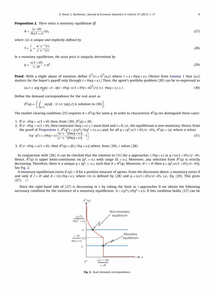
decreasing. Therefore, there is a unique q 2 ½qn,þ1Þ, such that A 2 AdðqÞ. Moreover, if r4 iy then q 2 ½qn,ðkð1þ iyÞÞ=ðr�iyÞ�.

See Fig. 2.A monetary equilibrium exists if zðjÞ40 for a positive measure of agents. From the discussion above, a monetary exists if

and only if r4 iy and Ao‘ðiÞ=yðqþkÞ, where ‘ðiÞ is defined by (28) and q¼ ðkð1þ iyÞÞ=ðr�iyÞ, i.e., Eq. (29). This gives(27). &

Since the right-hand side of (27) is decreasing in i, by taking the limit as i approaches 0 we obtain the followingnecessary condition for the existence of a monetary equilibrium: AocðynÞ=ðyðqnþkÞÞ. If this condition holds, (27) can be

A

Ad (q)

q* κ(1 + iθ)r−iθ

θ(q* + κ)c(y*)

(i)r−iθ

θκ(1+r)

A'

Non-monetaryequilibrium

Monetaryequilibrium

q

Fig. 2. Asset demand correspondence.

E. Nosal, G. Rocheteau / Journal of Economic Dynamics & Control 37 (2013) 1–1710

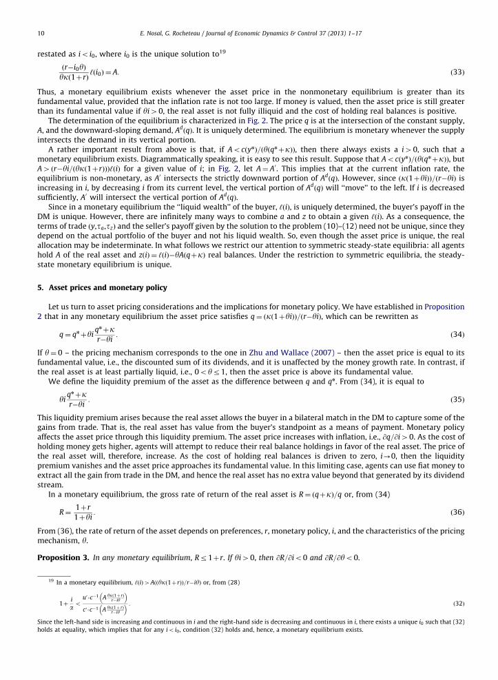
restated as io i0, where i0 is the unique solution to19

ðr�i0yÞykð1þrÞ

‘ði0Þ ¼ A: ð33Þ

Thus, a monetary equilibrium exists whenever the asset price in the nonmonetary equilibrium is greater than itsfundamental value, provided that the inflation rate is not too large. If money is valued, then the asset price is still greaterthan its fundamental value if yi40, the real asset is not fully illiquid and the cost of holding real balances is positive.

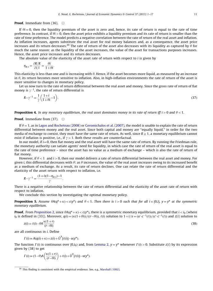
The determination of the equilibrium is characterized in Fig. 2. The price q is at the intersection of the constant supply,A, and the downward-sloping demand, Ad

ðqÞ. It is uniquely determined. The equilibrium is monetary whenever the supplyintersects the demand in its vertical portion.

A rather important result from above is that, if AocðynÞ=ðyðqnþkÞÞ, then there always exists a i40, such that amonetary equilibrium exists. Diagrammatically speaking, it is easy to see this result. Suppose that AocðynÞ=ðyðqnþkÞÞ, butA4 ðr�yi=ðykð1þrÞÞÞ‘ðiÞ for a given value of i; in Fig. 2, let A¼ A0. This implies that at the current inflation rate, theequilibrium is non-monetary, as A0 intersects the strictly downward portion of Ad

ðqÞ. However, since ðkð1þyiÞÞ=ðr�yiÞ isincreasing in i, by decreasing i from its current level, the vertical portion of Ad

ðqÞ will ‘‘move’’ to the left. If i is decreasedsufficiently, A0 will intersect the vertical portion of Ad

ðqÞ.Since in a monetary equilibrium the ‘‘liquid wealth’’ of the buyer, ‘ðiÞ, is uniquely determined, the buyer’s payoff in the

DM is unique. However, there are infinitely many ways to combine a and z to obtain a given ‘ðiÞ. As a consequence, theterms of trade ðy,ta,tzÞ and the seller’s payoff given by the solution to the problem (10)–(12) need not be unique, since theydepend on the actual portfolio of the buyer and not his liquid wealth. So, even though the asset price is unique, the realallocation may be indeterminate. In what follows we restrict our attention to symmetric steady-state equilibria: all agentshold A of the real asset and zðiÞ ¼ ‘ðiÞ�yAðqþkÞ real balances. Under the restriction to symmetric equilibria, the steady-state monetary equilibrium is unique.

5. Asset prices and monetary policy

Let us turn to asset pricing considerations and the implications for monetary policy. We have established in Proposition2 that in any monetary equilibrium the asset price satisfies q¼ ðkð1þyiÞÞ=ðr�yiÞ, which can be rewritten as

q¼ qnþyiqnþkr�yi

: ð34Þ

If y¼ 0 – the pricing mechanism corresponds to the one in Zhu and Wallace (2007) – then the asset price is equal to itsfundamental value, i.e., the discounted sum of its dividends, and it is unaffected by the money growth rate. In contrast, ifthe real asset is at least partially liquid, i.e., 0oyr1, then the asset price is above its fundamental value.

We define the liquidity premium of the asset as the difference between q and qn. From (34), it is equal to

yiqnþkr�yi

: ð35Þ

This liquidity premium arises because the real asset allows the buyer in a bilateral match in the DM to capture some of thegains from trade. That is, the real asset has value from the buyer’s standpoint as a means of payment. Monetary policyaffects the asset price through this liquidity premium. The asset price increases with inflation, i.e., @q=@i40. As the cost ofholding money gets higher, agents will attempt to reduce their real balance holdings in favor of the real asset. The price ofthe real asset will, therefore, increase. As the cost of holding real balances is driven to zero, i-0, then the liquiditypremium vanishes and the asset price approaches its fundamental value. In this limiting case, agents can use fiat money toextract all the gain from trade in the DM, and hence the real asset has no extra value beyond that generated by its dividendstream.

In a monetary equilibrium, the gross rate of return of the real asset is R¼ ðqþkÞ=q or, from (34)

R¼1þr

1þyi: ð36Þ

From (36), the rate of return of the asset depends on preferences, r, monetary policy, i, and the characteristics of the pricingmechanism, y.

Proposition 3. In any monetary equilibrium, Rr1þr. If yi40, then @R=@io0 and @R=@yo0.

19 In a monetary equilibrium, ‘ðiÞ4Aððykð1þrÞÞ=r�iyÞ or, from (28)

1þi

a ou03c�1 A ykð1þ rÞ

r�iy

� �c03c�1 A ykð1þ rÞ

r�iy

� � : ð32Þ

Since the left-hand side is increasing and continuous in i and the right-hand side is decreasing and continuous in i, there exists a unique i0 such that (32)

holds at equality, which implies that for any io i0, condition (32) holds and, hence, a monetary equilibrium exists.

E. Nosal, G. Rocheteau / Journal of Economic Dynamics & Control 37 (2013) 1–17 11

Proof. Immediate from (36). &

If yi¼ 0, then the liquidity premium of the asset is zero and, hence, its rate of return is equal to the rate of timepreference. In contrast, if yi40, then the asset price exhibits a liquidity premium and its rate of return is smaller than therate of time preference. The model predicts a negative correlation between the rate of return of the real asset and inflation.As inflation increases, agents substitute the real asset for real money balances and, as a consequence, the asset priceincreases and its return decreases.20 The rate of return of the asset also decreases with its liquidity as captured by y formuch the same reason: as the liquidity of the asset increases, the value of the asset for transactions purposes increases.Hence, the asset price increases and its return decreases.

The absolute value of the elasticity of the asset rate of return with respect to i is given by

ZR=i ¼@R=R

@i=i¼

yi

1þyi:

This elasticity is less than one and is increasing with y. Hence, if the asset becomes more liquid, as measured by an increasein y, its return becomes more sensitive to inflation. Also, in high-inflation environments the rate of return of the asset ismore sensitive to changes in monetary policy.

Let us now turn to the rate of return differential between the real asset and money. Since the gross rate of return of fiatmoney is g�1, the rate of return differential is

R�g�1 ¼1

g1þ i

1þyi�1

� : ð37Þ

Proposition 4. In any monetary equilibrium, the real asset dominates money in its rate of return iff i40 and yo1.

Proof. Immediate from (37). &

If y¼ 1, as in Lagos and Rocheteau (2008) or Geromichalos et al. (2007), the model is unable to explain the rate of returndifferential between money and the real asset. Since both capital and money are ‘‘equally liquid,’’ in order for the twomedia of exchange to coexist, they must have the same rate of return. As well, since RZ1, a monetary equilibrium cannotexist if inflation is positive, i.e., if g41. Both these results are counterfactual.

In our model, if i¼0, then fiat money and the real asset will have the same rate of return. By running the Friedman rule,the monetary authority can satiate agents’ need for liquidity, in which case the rate of return of the real asset is equal tothe rate of time preference – since the asset has no value as a medium of exchange – which is also the rate of return offiat money.

However, if yo1 and i40, then our model delivers a rate of return differential between the real asset and money. Forgiven i, this differential decreases with y: as y increases, the value of the real asset increases owing to its increased benefitas a medium of exchange. As a result, its rate of return declines. One can relate the rate of return differential and theelasticity of the asset return with respect to inflation, i.e.

R�g�1 ¼ð1þ iÞð1�ZR=iÞ�1

g :

There is a negative relationship between the rate of return differential and the elasticity of the asset rate of return withrespect to inflation.

We conclude this section by investigating the optimal monetary policy.

Proposition 5. Assume yAðqnþkÞocðynÞ and yo1. Then there is ı40 such that for all i 2 ½0,ı�, y¼ yn at the symmetric

monetary equilibrium.

Proof. From Proposition 2, since yAðqnþkÞocðynÞ, there is a symmetric monetary equilibrium, provided that io i0 (wherei0 is defined in (33)). Moreover, qðiÞ ¼ ðkð1þyiÞÞ=ððr�yiÞÞ, ‘ðiÞ solution to 1þ i=a¼ ðu03c�1ð‘ÞÞ=ðc03c�1ð‘ÞÞ and z(i) solution to

zðiÞ ¼ ‘ðiÞ�yAkð1þrÞ

ðr�yiÞð38Þ

are all continuous in i. Define

GðiÞ � AðqðiÞþkÞþzðiÞþUb½‘ðiÞ��uðynÞ:

The function GðiÞ is continuous over ½0,i0Þ and, from Lemma 2, y¼ yn whenever GðiÞ40. Substitute z(i) by its expressiongiven by (38) to get

GðiÞ � ð1�yÞAkð1þrÞ

ðr�yiÞ

� þ‘ðiÞþU

b½‘ðiÞ��uðynÞ:

20 This finding is consistent with the empirical evidence. See, e.g., Marshall (1992).

E. Nosal, G. Rocheteau / Journal of Economic Dynamics & Control 37 (2013) 1–1712

As i-0, ‘ðiÞ-cðynÞ and Ub½‘ðiÞ�-uðynÞ�cðynÞ. Since yo1

limi-0

GðiÞ ¼ ð1�yÞAkð1þrÞ

r40:

By continuity, there exists a nonempty interval ½0,ı� such that GðiÞ40. &

In most monetary models with a single asset, the Friedman rule is optimal and it achieves the first best (provided thatthere are no externalities, no distortionary taxes, and the pricing is well-behaved); we have that result too.21 However, incontrast to standard monetary models, a small deviation from the Friedman rule is neutral in terms of welfare in ourmodel. Hence, a small inflation is (weakly) optimal. The only effect of increasing the inflation above the Friedman rule is toincrease asset prices.

This finding has the following implications. First, a small inflation will have no welfare cost. Hence, we conjecture thatmoderate inflation (let say, 10%) will have a lower welfare cost than in standard models. Second, even though asset pricesrespond to monetary policy, these movements do not correspond to changes in society’s welfare. Hence, asset prices maynot be a very good indicator of society’s welfare or monetary policy effectiveness. Third, since there is a range of inflationrates that generates the first-best allocation, the optimal monetary policy is consistent with a rate of return differentialbetween fiat money and the real asset.

6. Liquidity structure of asset yields

In this section, we extend the model to allow for multiple real assets. We show that the same model that can explainthe rate of return dominance puzzle – that fiat money has a lower rate of return than risk-free bonds – can also deliver anon-degenerate distribution of asset yields despite agents being risk neutral. We will investigate how this structure ofyields is affected by monetary policy.

Suppose that there are a finite number KZ1 of infinitely lived real assets indexed by k 2 f1, . . . ,Kg. Denote Ak40 as thefixed stock of the asset k 2 f1, . . . ,Kg, kk its expected dividend, and qk its price. Agents learn the realization of the dividendof an asset at the beginning of the CM. Consequently, the terms at which the asset is traded in the DM only depend on theexpected dividend kk. Moreover, since agents are risk-neutral with respect to their consumption in the CM, the risk of anasset has no consequence for its price.22

Consider a buyer in the DM with a portfolio ðfakgKk ¼ 1,zÞ, where ak is the quantity of the kth real asset. The pricing

mechanism is a straightforward generalization of the one studied in the previous sections. The buyer’s payoff is given by

Ub¼ max

y,tm ,ftkguðyÞ�tm�

XK

k ¼ 1

tkðqkþkkÞ

" #ð39Þ

s:t: �cðyÞþtmþXK

k ¼ 1

tkðqkþkkÞZ0, ð40Þ

tmþXK

k ¼ 1

tkðqkþkkÞrzþXK

k ¼ 1

ykakðqkþkkÞ, ð41Þ

where yk 2 ½0,1� for all k. According to (39)–(41), the buyer’s payoff is the same as the one he would get in an economywhere he can make a take-it-or-leave-if-offer to the seller, but where he is constrained not to spend more than a fractionyk of the real asset k.

One can generalize Lemma 1 in the obvious way; in particular,

Ubð‘Þ ¼

uðynÞ�cðynÞ if ‘ZcðynÞ,

u3c�1ð‘Þ�‘ otherwise,

(ð42Þ

where ‘¼ zþPK

k ¼ 1 ykakðqkþkkÞ is the buyer’s liquid portfolio. Assume that y1Zy2Z � � �ZyK . Then,

ðqkþkkÞ�1 @U

b

@ak¼ yk

@Ub

@z:

So 1=ðqkþkkÞ units of the kth asset, which yields one unit of CM output, allows the buyer to raise his surplus in the DM bya fraction yk of what he would obtain by accumulating one additional unit of real balances instead. The parameter yk canthen be interpreted as a measure of the liquidity of the asset k, that is, the extent to which it can be used to finance

21 In search monetary models, the Friedman rule can be suboptimal because of search externalities (Rocheteau and Wright, 2005) or distortionary

taxes (Aruoba and Chugh, 2010). Also, if the coercive power of the government is limited, then the Friedman rule might not be incentive-feasible (Hu

et al., 2009; Andolfatto, 2010).22 The result that the price of an asset does not depend on its risk would no longer be true if the realization of the dividend was known in the DM

when agents trade in bilateral matches. See Lagos (2010) and Rocheteau (2011).

E. Nosal, G. Rocheteau / Journal of Economic Dynamics & Control 37 (2013) 1–17 13

consumption opportunities in the DM at favorable terms of trade. Given our ranking, the asset 1 is the most liquid and theasset K is the least.

The second step of the pricing procedure is a generalization of (10)–(12). The seller’s payoff and the actual terms oftrade are determined by

Us¼ max

y,tm ,ftkg�cðyÞþtmþ

XK

k ¼ 1

tkðqkþkkÞ

" #

s:t: uðyÞ�tm�XK

k ¼ 1

tkðqkþkkÞZUb

�zsrtmrz, �askrtkrak, k¼ 1, . . . ,K :

In the CM agents choose the portfolio, ðfakg,zÞ, that they will bring into the DM. The portfolio problem is

ðfakg,zÞ 2 arg maxfakg,z

�iz�rXK

k ¼ 1

akðqk�qn

kÞþaUb

zþXK

k ¼ 1

ykakðqkþkkÞ

!( ), ð43Þ

and qn

k ¼ kk=r. According to (43), the agent maximizes his expected utility of being a buyer in the DM, net of the cost of theportfolio. The cost of holding asset k is the difference between the price of the asset and its fundamental value (expressedin flow terms), while the cost of holding real balances is i¼ ðg�bÞ=b, approximately the sum of the inflation rate and therate of time preference. An agent’s portfolio choice problem, (43), can be rewritten as

maxfakg,‘

�i‘þXK

k ¼ 1

ak½iykðqkþkkÞ�rðqk�qn

kÞ�þaUbð‘Þ

( )ð44Þ

s:t:XK

k ¼ 1

ykakðqkþkkÞr‘: ð45Þ

As in Section 4, in a monetary equilibrium, constraint (45) does not bind, ‘ solves (28), and the asset prices must satisfyiykðqkþkkÞ�rðqk�qn

kÞ ¼ 0 or

qk ¼1þ iyk

r�iykkk, 8k 2 f1, . . . ,Kg, ð46Þ

for all k 2 f1, . . . ,Kg.23 Note that the price of real asset k increases with inflation, provided that yk40. From (45) and (46), amonetary equilibrium exists if r4 iyk for all k and

XK

k ¼ 1

ykAk1þr

r�iyk

� kko‘ðiÞ: ð47Þ

For money to be valued, the total stock of real assets, adjusted by their liquidity factors, must not be too large. The rate ofreturn of asset k is given by

Rk ¼kkþqk

qk

¼1þr

1þ iyk, 8k 2 f1, . . . ,Kg: ð48Þ

Provided that the nominal interest rate is strictly positive, the model is able to generate differences in the rates of return ofthe real assets, where the ordering depends on the liquidity coefficients fykg.

Proposition 6. In any monetary equilibrium, RK ZRK�1Z � � �ZR1Zg�1. Moreover,

Rk0�Rk ¼ ð1þrÞiðyk�yk0 Þ

ð1þ iykÞð1þ iyk0 Þ40: ð49Þ

Proof. Direct from (48). &

The differences between the rates of return across assets emerge even if the assets are risk-free, or agents are risk-neutral. These differences arise because the pricing mechanism has different assets being traded at different terms of tradein the DM. These rate-of-return differences would be viewed as anomalies by standard consumption-based asset pricingtheory.

Let us turn to monetary policy. A change in inflation affects the entire structure of asset returns. Denote fRikg

Kk ¼ 1 the

structure of asset yields when the cost of holding fiat money is equal to i.

23 The proof to these claims are almost identical to the proof of Proposition 2. Specifically, if rðqk�qn

kÞ4 iykðqkþkkÞ, then AdðqkÞ ¼ f0g, which cannot be

an equilibrium; if rðqk�qn

kÞo iykðqkþkkÞ, then constraint (45) binds and z¼0, i.e., the equilibrium is non-monetary; and if rðqk�qn

kÞ ¼ iykðqkþkkÞ, thenPkAd

kðqkÞykðqkþkkÞ 2 ½0,‘�, where ‘ solves (28).

E. Nosal, G. Rocheteau / Journal of Economic Dynamics & Control 37 (2013) 1–1714

Proposition 7. In any monetary equilibrium, fRikg

Kk ¼ 1 dominates fRi0

kgKk ¼ 1 in a first-order stochastic sense whenever i04 i.

Moreover, ð@ðRk0�RkÞÞ=@i40 if and only if ðyk�yk0 Þð1�i2ykyk0 Þ40.

Proof. The first part of the proposition is direct from (48). From (49), if yk ¼ yk0 then Rk0�Rk ¼ 0 which is independent of i.Without loss of generality, assume yk4yk0 and i40 so that Rk0�Rk40. From (49), differentiate lnðRk0�RkÞ to get

@ lnðRk0�RkÞ

@i¼

1�i2ykyk0

ið1þ iykÞð1þ iyk0 Þ: &

An increase in inflation raises the rates of return of all real assets because agents substitute the real assets for realbalances which are more costly to hold. Moreover, the premia paid to the less liquid assets, Rk0�Rk with yk4yk0 , increaseprovided that i is not too large. So if one interpret the less liquid asset as risky equity and the most liquid one as risk-freebonds, then the equity premium increases with inflation.

7. Conclusion

The main contribution of this paper is to show that the rate-of-return-dominance and other asset pricing puzzles neednot be puzzles when viewed through the lens of monetary models with bilateral trades. These seemingly anomalous assetpricing patterns can be generated by trading mechanisms that are Pareto-efficient and that do not impose any restrictionon the use of assets as means of payment, i.e., the Wallace (1996) dictum is satisfied. Liquidity differences across assets canarise because agents coordinate on a mechanism that makes it cheaper for buyers to trade some assets relative to others.For instance, sellers can agree to offer better terms of trade to buyers trading with money instead of bonds or equity. Lagos(2010) shows that a calibrated version of a search-theoretic monetary model can account for both the risk-free rate andthe equity premium puzzles once a small restriction is introduced on the use of equity as means of payment. Our analysisindicates that such a restriction is, in fact, not needed once one allows for a broader class of trading mechanisms. Thetrading mechanism we have considered has strategic foundations, which can be found in the appendix.

Appendix A. Strategic foundations for the 2-step procedure

We describe a two-stage bargaining game with perfect information between a buyer and a seller. The buyer has z realbalances and a real assets, and the seller has zs real balances and as real assets. The agents’ portfolios are commonknowledge. In the first stage, the buyer puts a fraction 1�y of his real assets on the bargaining table, and agents bargainover the number of these real assets that will be transferred to the seller and the amount of output the seller will producefor the buyer. In the second stage, the buyer puts the rest of his assets on the bargaining table, i.e., all his real balances anda fraction y of his real assets, and agents bargain over the transfer of assets to the seller and the amount of output the sellerproduces. The fraction 1�y of the buyer’s real assets that are on the negotiation table in the first stage cannot be used inthe second stage negotiation. For example, if the first stage results in no output being produced and no real assets beingexchanged, then, even though the buyer has a real assets going into the second stage, he can only use the ya of them atthat time.

The seller makes a take-it-or-leave-it offer in the first stage, and the buyer makes a take-it-or-leave-it offer in thesecond stage. Without loss of generality, we assume that the seller does not transfer any of his assets. Here is the game thatagents play.

STAGE 1.

The seller makes an offer ðy1,t1a Þ, where y1 2 Rþ is output the seller will produce and t1

a 2 ½0,ð1�yÞa� is theamount of real assets the buyer must transfer to the seller. The buyer accepts (Y) or rejects (N) the offer. If theoffer is accepted, then the production/consumption of the good and the transfer of real assets take place.

STAGE 2.

The buyer makes an offer ðy2,t2a ,t2

mÞ, where y2 2 Rþ is output, t2mr ½0,z� is a transfer of real balances and t2

a 2

½0,ya� is a transfer of real assets. The seller accepts (Y) or rejects (N) the offer. If the offer is accepted, theproduction/consumption of the good and the transfer of real balances and assets take place.

The buyer’s payoff is

uðy1þy2ÞþWða�t1a�t

2a ,z�t2

mÞ,

where the consumption goods in the two stages of the game are perfect substitutes. The seller’s payoff is

�cðy1þy2ÞþWðasþt1aþt

2a ,zsþt2

mÞ:

The game tree is represented in Fig. 3. The base of each triangle represents the continuum of offers that an agentcan make.

A strategy for the buyer is acceptance rule that specifies the set of offers in the first stage that are acceptable, and anoffer – over output, real balances and real balances – in the second stage that is a function of the offer made by the seller in

Fig. 3. Game tree.

E. Nosal, G. Rocheteau / Journal of Economic Dynamics & Control 37 (2013) 1–17 15

the first stage and whether the offer was accepted or rejected. A strategy for the seller is an offer – over output and realassets – in the first stage and an acceptance rule in the second stage. The equilibrium concept is subgame perfection.

The game is solved by backward induction. Consider a subgame following a first stage offer ðy1,t1aÞ. Without loss of

generality, assume that the offer is accepted. If it is rejected, set ðy1,t1aÞ ¼ ð0,0Þ. The buyer’s problem in the second stage of

the game is

Ubðy1,t1aÞ ¼ max

y2 ,t2a ,t2

m

½uðy1þy2ÞþWða�t1a�t

2a ,z�t2

mÞ� ð50Þ

s:t: �cðy1þy2ÞþWðasþt1aþt

2a ,zsþt2

mÞZ�cðy1ÞþWðasþt1a ,zsÞ, ð51Þ

t2a rya, t2

mrz: ð52Þ

According to (50), the buyer chooses a quantity of output, y2, and a transfer of real balances and real assets, t2m and t2

a ,respectively, to maximize his payoff taking as given the trade that took place in the first stage of the game. The seller’sacceptance rule in the second stage is given by (51). The seller must obtain a payoff that is at least as large as the payoff heobtains if he rejects the offer. In case of indifference, we assume that the seller accepts the offer so that the buyer’sproblem has a solution. The disagreement payoff is the utility associated with the trade ðy1,t1

aÞ in the first stage, and notrade in the second stage, i.e., y2 ¼ t2

m ¼ t2a ¼ 0. Since the buyer’s payoff is decreasing in t2

m and t2a , and the seller’s payoff is

increasing in t2m and t2

a , it is immediate that (51) holds at equality. If this were not the case, the buyer would have aprofitable deviation by reducing t2

m or t2a . From the linearity of W, (51) reduces to t2

mþðqþkÞt2a ¼ cðy1þy2Þ�cðy1Þ. The

transfer of assets compensates the seller for the disutility of producing y2 units of output, given that y1 units were alreadyproduced in the first stage. Finally, (52) are feasibility constraints that say the buyer cannot offer more real balances thanhe holds and more real assets that are on the bargaining table.

Using the linearity of W, the buyer’s problem can be rewritten as

Ubðy1,t1aÞ ¼max

y2

½uðy1þy2Þ�cðy1þy2Þ�þcðy1ÞþWða�t1a ,zÞ ð53Þ

s:t: cðy1þy2Þ�cðy1ÞrzþðqþkÞya: ð54Þ

The objective function in (53) is strictly concave in y2, and (54) defines a closed interval for the choice of y2. The uniquesolution to (53)–(54) is y2 ¼ 0 if y1Zyn, y2 ¼ yn�y1 if y1oyn and cðynÞ�cðy1ÞrzþðqþkÞya, and cðy1þy2Þ�cðy1Þ ¼

zþðqþkÞya otherwise. If the output produced in the first stage of the game is larger than the efficient quantity, thenno trade takes place. Otherwise, the buyer asks the seller to complement his first-stage production so that total productionis either efficient or as large as possible if less than efficient.

The buyer’s payoff, taking as given the trade in the first stage of the game, is

Ubðy1,t1aÞ ¼

uðy1ÞþWða�t1a ,zÞ if y1Zyn,

uðynÞ�cðynÞþcðy1ÞþWða�t1a ,zÞ if cðy1Þ 2 ½cðy

nÞ�z�yðqþkÞa,cðynÞÞ,

u3c�1½cðy1ÞþzþyðqþkÞa��z�yðqþkÞaþWða�t1a ,zÞ if cðy1ÞocðynÞ�z�yðqþkÞa:

8><>: ð55Þ

The buyer’s payoff is increasing in y1, and Ubðy1,t1aÞ ¼ Ubðy1,0Þ�ðqþkÞt1

a .

E. Nosal, G. Rocheteau / Journal of Economic Dynamics & Control 37 (2013) 1–1716

Let’s move up in the game tree. In the first stage, the seller’s problem is

maxy1 ,t1

a

f�c½y1þy2ðy1,t1aÞ�þW ½asþt1

aþt2a ðy1,t1

aÞ,zsþt2

mðy1,t1aÞ�g ð56Þ

s:t: Ubðy1,t1aÞZUbð0,0Þ: ð57Þ

t1a r ð1�yÞa: ð58Þ

According to (56), the seller chooses a level of production, y1, and a transfer of real assets, t1a , to maximize his payoff. In

doing so, the seller takes as given the buyer’s strategy in the second stage of the game, as represented by the solution of(50)–(52). This means that the second-stage offer by the buyer, ðy2,t2

m,t1a Þ, depends on the seller’s offer in the first stage.

According to (57), the buyer accepts the seller’s offer if it generates a payoff at least as large as the one he would get if herejects the offer. The disagreement payoff, Ubð0,0Þ, is the payoff that the buyer receives in the second stage assuming thatno trade takes place in the first stage. Finally, (58) is a feasibility constraint on the transfer of real assets, i.e., one cannottransfer more real assets than there are on the bargaining table.

We can simplify the seller’s problem (56)–(58). From (51) at equality, the seller’s payoff what he would obtain if notrade takes place in the second stage of the bargaining game, �cðy1ÞþWðasþt1

a ,zsÞ. Moreover, given that the seller’s payoffis decreasing in y1 and Ubðy1,t1

aÞ is increasing in y1, (11) must hold at equality, i.e., Ubðy1,t1a Þ ¼ Ubð0,0Þ. So, the buyer obtains

the same payoff he would obtain when he is constrained to use at most a fraction y of his real assets. From these twoobservations, the seller’s problem can be rewritten as

maxy1

½Ubðy1,0Þ�cðy1Þ�þWðas,zsÞ�Ubð0,0Þ ð59Þ

s:t: Ubðy1,0Þr ð1�yÞðqþkÞaþUbð0,0Þ: ð60Þ

From (55),

Ubðy1Þ ¼

uðy1Þ�cðy1ÞþWða,zÞ if y1Zyn,

uðynÞ�cðynÞþWða,zÞ if cðy1Þ 2 ½cðynÞ�z�yðqþkÞa,cðynÞÞ,

u3c�1½cðy1ÞþzþyðqþkÞa��cðy1Þ�z�yðqþkÞaþWða,zÞ if cðy1ÞocðynÞ�z�yðqþkÞa,

8><>:

where Ubðy1Þ ¼ Ubðy1,0Þ�cðy1Þ. Suppose feasibility constraint (60) does not bind. The solution to (59)–(60) is y1 that

maximizes Ubðy1Þ. It is easy to check that

maxy1

Ubðy1Þ ¼ uðynÞ�cðynÞþWða,zÞ:

If cðynÞ4zþyðqþkÞa, then any y1 2 ½c�1½cðynÞ�z�yðqþkÞa�,yn� is a solution. If cðynÞrzþyðqþkÞa, then any y1 2 ½0,yn� is a

solution. From (55) the feasibility constraint, (60), is satisfied if

uðynÞþWð0,0ÞrUbð0,0Þ when zþyðqþkÞaocðynÞ or ð61Þ

uðynÞ�cðynÞþWða,zÞr ð1�yÞðqþkÞaþUbð0,0Þ when zþyðqþkÞaZcðynÞ, ð62Þ

where, from (55),

Ubð0,0Þ ¼ uðynÞ�cðynÞþWða,zÞ if zþðqþkÞyaZcðynÞ ð63Þ

Ubð0,0Þ ¼ u3c�1½zþyðqþkÞa��z�yðqþkÞaþWða,zÞ if zþðqþkÞyaocðynÞ: ð64Þ

We can distinguish three cases:

1.

zþyðqþkÞaZcðynÞ:

It is immediate from (63) that (62) is satisfied. One solution to the two stage bargaining game is that the seller makesno offer in the first stage,and the buyer offers y2 ¼ yn and t2

mþðqþkÞt2a ¼ cðynÞ in the second stage,which the seller

accepts. The seller’s payoff is Wðas,zsÞ and the buyer’s payoff is uðynÞ�cðynÞþWða,zÞ.

2. zþyðqþkÞaocðynÞ and ð1�yÞðqþkÞaZuðynÞ�u3c�1½zþyðqþkÞa�.

It can be checked from (64) that (61) is satisfied. One solution to the two stage bargaining game is that the seller offersy1 ¼ c�1½cðynÞ�z�yðqþkÞa� and t1

a ¼ ðuðynÞ�u3c�1½zþyðqþkÞa�Þ=ðqþkÞ in the first stage,which the buyer accepts; in

the second stage the buyer offers y2 ¼ yn�y1 and t2m ¼ z and t2

a ¼ ya, which the seller accepts. The seller’s payoff isuðynÞ�cðynÞ�½u3c�1½zþyðqþkÞa��z�yðqþkÞa�þWðas,zsÞ and the buyer’s payoff is u3c�1½zþyðqþkÞa��z� yðqþkÞaþWða,zÞ.

3.

zþyðqþkÞaocðynÞ and ð1�yÞðqþkÞaouðynÞ�u3c�1½zþyðqþkÞa�.In this case, feasibility condition (61) is not satisfied. From (55) and (60) at equality, we get

u3c�1½cðy1ÞþzþyðqþkÞa� ¼ ð1�yÞðqþkÞaþu3c�1½zþyðqþkÞa�: ð65Þ

E. Nosal, G. Rocheteau / Journal of Economic Dynamics & Control 37 (2013) 1–17 17

The unique solution to the two stage bargaining game is that the seller offers the y1 implicitly defined by (65) andt1

a ¼ ð1�yÞa in the first stage, which the buyer accepts; in the second stage, (from (53) to (54)), the buyer offers t2m ¼ z,

t2a ¼ ya, and cðy1þy2Þ�cðy1Þ ¼ zþyðqþkÞa, which the seller accepts. The seller’s payoff is uðy1þy2Þ�cðy1þy2Þ�

½u3c�1½zþyðqþkÞa��z�yðqþkÞa�þWðas,zsÞ and the buyer’s payoff is u3c�1½zþyðqþkÞa��z�yðqþkÞaþWða,zÞ.

Let us compare the solution to this game to the solution to the trading mechanism in the main body of the paper.

1.

zþyðqþkÞaZcðynÞ.From Lemma 1, the buyer’s surplus is uðynÞ�cðynÞ, and from Lemma 2, y¼ yn and tmþtaðqþkÞ ¼ cðynÞ.

2.

zþyðqþkÞaocðynÞ and ð1�yÞðqþkÞaZuðynÞ�u3c�1½zþyðqþkÞa�.From Lemma 1, the buyer’s surplus is u3c�1½zþyðqþkÞa��z�yðqþkÞa, and from Lemma 2, y¼ yn andtmþtaðqþkÞ ¼ uðynÞ�u3c�1½zþyaðqþkÞ�þzþyaðqþkÞ.

3.

zþyðqþkÞaocðynÞ and ð1�yÞðqþkÞaZuðynÞ�u3c�1½zþyðqþkÞa�.From Lemma 1, the buyer’s surplus is u3c�1½zþyðqþkÞa��z�yðqþkÞa, and from Lemma 2, ta ¼ a, tm ¼ z, anduðyÞ ¼ ð1�yÞaðqþkÞþu3c�1½zþyaðqþkÞ�.

It is easy to check that the solution to the two-round bargaining game is also a solution to the trading mechanism usedin the main text.

References

Andolfatto, D., 2010. Essential interest-bearing money. Journal of Economic Theory 145, 1319–1602.Aruoba, S.B., Chugh, S.K., 2010. Optimal fiscal and monetary policy when money is essential. Journal of Economic Theory 145, 1618–1647.Aruoba, S.B., Schorfheide, F., 2010. An Estimated Search-Based Monetary DSGE Model with Liquid Capital. Working Paper.Aruoba, S.B., Wright, R., 2003. Search, money and capital: a neoclassical dichotomy. Journal of Money, Credit and Banking 35, 1086–1105.Aruoba, S.B., Rocheteau, G., Waller, C., 2007. Bargaining and the value of money. Journal of Monetary Economics 54, 2636–2655.Banarjee, A., Maskin, E., 1996. A Walrasian theory of money and barter. Quarterly Journal of Economics 111, 955–1005.Bansal, R., Coleman, J., 1996. A monetary explanation of the equity premium, term premium, and risk-free rate puzzles. Journal of Political Economy 104,

1135–1171.Duffie, D., Garleanu, N., Pedersen, L.H., 2005. Over-the-counter markets. Econometrica 73, 1815–1847.Geromichalos, A., Licari, J.M., Suarez-Lledo, J., 2007. Monetary policy and asset prices. Review of Economic Dynamics 10, 761–779.Hu, T.-W., Kennan, J., Wallace, N., 2009. Coalition-proof trade and the Friedman rule in the Lagos–Wright model. Journal of Political Economy 117,

116–137.Kiyotaki, N., Moore, J., 2005. Liquidity and asset prices. International Economic Review 46, 317–349.Kiyotaki, N., Wright, R., 1989. On money as a medium of exchange. Journal of Political Economy 97, 927–954.Lagos, R., 2010. Asset prices and liquidity in an exchange economy. Journal of Monetary Economics 57, 913–930.Lagos, R., Rocheteau, G., 2008. Money and capital as competing media of exchange. Journal of Economic Theory 142, 247–258.Lagos, R., Wright, R., 2005. A unified framework for monetary theory and policy analysis. Journal of Political Economy 113, 463–484.Lester, B., Postlewaite, A., Wright, R., 2012. Information, liquidity, asset prices and monetary policy. Review of Economic Studies 79, 1209–1238.Marshall, D., 1992. Inflation and asset returns in a monetary economy. Journal of Finance 47, 1315–1342.O’Neill, B., Samet, D., Wiener, Z., Winter, E., 2004. Bargaining with an agenda. Games and Economic Behavior 48, 139–153.Rocheteau, G., Wright, R., 2005. Money in search equilibrium, in competitive equilibrium, and in competitive search equilibrium. Econometrica 73,

175–202.Rocheteau, G., 2011. Payments and liquidity under adverse selection. Journal of Monetary Economics 58, 191–205.Shi, S., 1997. A divisible search model of fiat money. Econometrica 65, 75–102.Wallace, N., 1996. A dictum for monetary theory. Federal Reserve Bank of Minneapolis Quarterly Review 22, 20–26.Wallace, N., 2000. A model of the liquidity structure based on asset indivisibility. Journal of Monetary Economics 45, 55–68.Weill, P.-O., 2008. Liquidity premia in dynamic bargaining markets. Journal of Economic Theory 140, 66–96.Williamson, S., Wright, R., 1994. Barter and monetary exchange under private information. American Economic Review 84, 104–123.Zhu, T., Wallace, N., 2007. Pairwise trade and coexistence of money and higher-return assets. Journal of Economic Theory 133, 524–535.