Abstract—Supporting effective load balancing is paramountfor increasing network utilization efficiency and improving theperceivable user experience in emerging and future cellularnetworks. At the same time, it is becoming increasinglyalarming that current communication practices lead to ex-cessive energy wastes both at the infrastructure side andat the terminals. To address both these issues, this paperdiscusses an innovative communication approach enabled bythe implementation of device-to-device (d2d) communicationover cellular networks. The technique capitalizes on the delaytolerance of a significant portion of Internet applicationsand the inherent mobility of the nodes to achieve significantperformance gains. For delay tolerant messages, a mobile nodecan postpone message transmission − in a store-carry andforward manner − for a later time to allow the terminal toachieve communication over a shorter range or to postponecommunication to when the terminal enters a cooler cell,before engaging in communication. Based on this framework,a theoretical model is introduced to study the generalizedmultihop d2d forwarding scheme where mobile nodes areallowed to buffer messages and carry them while in transit.Thus, a multi-objective optimization problem is introducedwhere both the communication cost and varying load levelsof multiple cells are to be minimized. We show that themathematical programming model that arises can be solvedefficiently in time. Further, extensive numerical investigationsreveal that the proposed scheme is an effective approachfor both energy efficient communication as well as offeringsignificant gains in terms of load balancing in multicelltopologies.
Index Terms—Load balancing, Energy efficiency, Storecarry and forward relaying, Device to device communication,Wireless routing, Cellular networks.
I. INTRODUCTION
With the increasingly high availability of rich contentInternet applications on mobile devices and more recentlyvehicular terminals (which are driven by user demand), datause surging is expected to increase, severely compromisingsystem performance and eventually (as a by-product) over-all user experience. Residing on the supporting neighboringcells of hot-spot areas to alleviate the problem, numeroustechniques are proposed in the literature to either decide onthe initial user association policies [1]-[4], cell reselectionalgorithms [5]-[8] or network-driven handover procedures
∗Department of Informatics, Centre for Telecommuni-cations Research, King’s College London, Strand, WC2R2LS, London, England, e-mail:∗panayiotis.kolios,‡[email protected]
†Department of Mathematics, London School of Economics,Houghton Street, London WC2A 2AE, London, England, e-mail:[email protected] received ...
[9]. However, the majority of these techniques has as asalient assumption real-time constraints on the requestedtraffic and thus decisions are made on the instantaneouscell loading conditions. In [10] batch processing of datarequests is considered; illustrating the potential load bal-ancing improvements that can be achieved by collectivelyconsidering the load assignment problem over the availableinfrastructure nodes. In contrast to the latter work, hereafterwe labour a broader range of message delivery delayswhere elastic services can handle delays in the order offew seconds with no degradation in the perceivable userexperience. In that respect, a mobile node (e.g. vehicularterminal) could potentially postpone communication for alater time instance when it enters the serving area of aneighboring cell, in effect reducing the load imbalanceacross the network. Further, by postponing communica-tion a mobile node can approach closer to the servinginfrastructure node before initiating the transmission andhence reducing the physical (Euclidean) communicationdistance that compromises communication. Therefore, boththe inter-cell load levels and intra-cell energy consumptioncan be reduced by exploiting the available message deliverydelays and exploring the feasible forwarding paths that canbe formed by the mobile nodes. Energy reduction in bothuser terminals as well as the network as a whole is ofcritical importance and the proposed technique, that allowslocalized transmission, can assist towards this aim.
A. Background and Related Work
Node mobility has been previously considered as a keyelement to achieve communication in intermittently con-nected networks (i.e., Delay Tolerant Netwoks)[11][12], toincrease the capacity of ad-hoc and cellular networks ([13]and [14] respectively) and to improve the energy efficiencyby reducing the physical communication distance betweencommunicating nodes [15]-[17]. In this work we investigatean additional benefit branching as a result of mobility anddelay tolerance; that of energy efficient load balancing incellular systems. Notably, by postponing communication,a mobile node can carry information while in transit andopt for a better serving cell with favourable load condi-tions. Hence, communication can be achieved via a store-carry and forwarding (SCF) paradigm under the deadlineconstraints imposed by the initiated service. Note that theSCF scheme considered hereafter differs drastically fromthe ones previously proposed for delay tolerant networks(DTNs). Firstly in DTNs, and due to the absence of end-
2
to-end connectivity, information is stored by nodes and op-portunistically forwarded at node encounters. Here, due tothe presence of the infrastructure network, all nodes are ableto communicate directly with at least one base station (BS)and thus timely deliveries can be guaranteed. Secondly, inDTNs due to the unpredictable mobility patterns, messagesare replicated at node encounters (in a broadcast or moreintelligent manner) to increase the probability for successfulcommunication. For the applications we consider here,informed routing decisions are made by the infrastructureunits that have instantaneous knowledge regarding all nodepositions within the coverage area of the BSs. The proposedload balancing scheme will be further propelled as deviceto device (d2d) communication will be a supported featurein LTE Release 12 and beyond.
B. Paper contributions
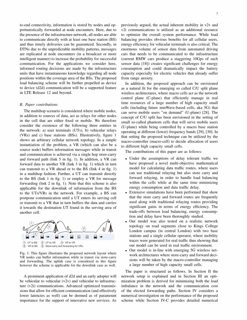
The multihop scenario is considered where mobile nodes,in addition to sources of data, act as relays for other nodesin the cell that are either fixed or mobile. We thereforeconsider the existence of the following three entities inthe network: a) user terminals (UTs), b) vehicular relays(VRs) and c) base stations (BSs). Illustratively, figure 1shows an arbitrary cellular network topology. In a simpleinstantiation of the problem, a VR (which can also be asource node) buffers information messages while in transitand communication is achieved via a single hop store-carryand forward path (link 5 in fig. 1). In addition, a VR canforward data to another VR (link 3 in fig. 1) which in turncan transmit to a VR ahead or to the BS (link 4 in fig. 1)in a multihop fashion. Further, a UT can transmit directlyto the BS (link 1 in fig. 1) or employ a VR for messageforwarding (link 2 in fig. 1). Note that this scheme is alsoapplicable for the downlink of information from the BSto the UTs/VRs in the network. For example, a BS canpostpone communication until a UT enters its serving cellor transmit to a VR that in turn buffers the data and carriesit towards the destination UT found in the serving area ofanother cell.
1
52
4
3
1 UT to BS 2 UT to VR
4 VR to BS 5 Store-carry and forwarding for VRs
3 VR to VR
Fig. 1: This figure illustrates the proposed network layout whereVR nodes can buffer information while in transit via store-carryand forwarding. The uplink case is considered in this figurehowever the scheme is applicable for the downlink case as well.
A prominent application of d2d and an early adopter willbe vehicular to vehicular (v2v) and vehicular to infrastruc-ture (v2i) communications. Advanced optimized transmis-sions that allow for efficient communication (and effectivelylower latencies as well) can be deemed as of paramountimportance for the support of innovative new services. As
previously argued, the actual inherent mobility in v2v andv2i communications is utilized as an additional resourceto optimize the overall system performance. While loadbalancing provides obvious benefits for all cellular users,energy efficiency for vehicular terminals is also critical. Theenormous volume of sensor data from automated drivingcars that needs to be communicated to the infrastructure(current BMW cars produce a staggering 10Gps of suchsensor data [18]) creates significant challenges for energyconsumption and could dramatically impact the batterycapacity especially for electric vehicles that already sufferfrom range anxiety.
In addition, the proposed approach can be envisionedas a natural fit for the emerging so called C/U split planewireless architectures, where macro cells act as the networkcontrol plane (C-plane) that efficiently manage in realtime resources of a large number of high capacity smallcells (including future mmWave-based cells, aka 5G) thatcan serve mobile users ”on demand” (U-plane) [28]. Theconcept of C/U split has been envisioned in the setting ofsmall so-called phantom cells that will serve mobile users(U-plane) while being controlled by a macro base stationoperating at different (lower) frequency bands [29], [30]. Inthat setting the proposed technique can be utilized by themacro-controller (macro-cell) to decide allocation of usersto different high capacity small cells.
The contributions of this paper are as follows:
• Under the assumptions of delay tolerant traffic wehave proposed a novel multi-objective mathematicalmodel for calculating data traffic routes, where userscan use traditional relaying but also store carry andforward relaying, in order to handle load balancingwithin the cells while at the same time minimizingenergy consumption and data traffic delay.
• Extensive simulations have been performed that showthat the store carry and forward routes are frequentlyused along with traditional relaying routes providingsignificant gains in terms of energy efficiency. Thetrade-offs between load balancing, energy consump-tion and delay have been thoroughly studied.
• Our model was also tested on a realistic networktopology on road segments close to Kings CollegeLondon campus (in central London) with two basestations and a single cellular operator, where mobilitytraces were generated for real traffic thus showing thatour model can be used in real traffic environment.
• Our model is in-line with emerging 5G wireless net-work architectures where store-carry and forward deci-sions will be taken by the macro-controller managinga large number of high capacity small cells.
The paper is structured as follows. In Section II thenetwork setup is explained and in Section III an opti-mization problem is derived for minimizing both the loadimbalance in the network and the communication costof the elected forwarding paths. Section IV considers anumerical investigation on the performance of the proposedscheme while Section IV-C provides detailed numerical
3
investigations for different network setups. Finally, SectionVI concludes the paper.
II. SYSTEM MODEL
In this section we first consider the network structure un-der investigation and define the communication model andload balancing models. Table I contains variable definitionsto be used as a reference for the derivations that follow.
We consider the uplink case of cellular operation, how-ever the model is applicable to the downlink case asexplained above. A constellation of C = {1, . . . , C} cellsis considered each with cell radius of R meters. Forillustration reasons we initially assume a 1-dimensionalrealization of the network topology, and more general casesare considered in section IV-C. Further, M = {1, . . . ,M}uniformly distributed users are considered to be activewhile N = {1, . . . , N} relay nodes travel along eachdirection of a bi-directional stretch of road. To differentiatebetween source and relay nodes we assume that all users(source nodes) are static or slow moving and thus theirposition does not change abruptly. Note that this assumptiondoes not restrict the model in any way, any node can beconsidered as a source node in general and the model isstill applicable. Finally, with vj we denote the velocity ofmobile node j ∈ N .
A. Communications ModelFor the communication model we assume that all nodes
can transmit and receive from a single other node at anytime instance. All users have a single message of F (bits) tocommunicate to the BS (the case of variable size messagesis considered in appendix B) and all links are able totransmit at a data rate of B (bps). We further considerthree sources of energy consumption: 1) the circuit energyconsumption at the transmitter side, et, 2) the energyconsumed to receive a message at the receiver, er and 3) theenergy consumed by the power amplifier at the transmitterside, ed. Large scale propagation losses are consideredwith signal attenuations following a two-stage model. Fortransmission distances less than a threshold distance dbrake,the free space model is considered, while for large distancesthe plane-earth model is employed.
The physical distance between communicating nodesmay change during transmission as some nodes are mo-bile. We define vij to be the relative velocity betweencommunicating nodes i, j. Also Dij is the initial distancebetween the transceiver pair i, j. With g(Dij , t) we denotethe absolute distance at time t between the transceiver pairi, j during transmission and is defined as follows:
g(Dij , t) = |Dij − vijt|. (1)
Based on the above equation, the total energy consump-tion between nodes i and j can be computed as follows:
fij = (er + et)Bτ +Bed
∫ τ
0
g(Dij , t)ηdt, (2)
where τ = F/B is the communication time and ηexpresses the pathloss exponent.
B. Load Balancing Model
Balancing the load across the C BSs is equivalent tominimizing the variance of these loads. We let Sk be theinitial load (for example in bps) for each k ∈ C, q be theincrease in rate of accepting each user request, and Uk bethe maximum capacity in terms of rate at BS k. We defineinteger variables yk to be the total number of user requestsaccepted by BS k, and let binary variables zmk take thevalue 1 only if user m is satisfied by BS k.
Using the above notation, the variance between the loadsat the different BSs after accepting the requests is asfollows:
Var =C∑
k=1
[ykq + Sk −
∑Cj=1(yjq + Sj)
C
]2(3)
where the new load at BS j is yjq + Sj . To balance theload between BSs, we formulate the following optimisationproblem:
(P1)min Var (4)
s.t.
C∑k=1
zmk = 1 ∀m ∈ M (5)
M∑m=1
zmk = yk ∀ k ∈ C (6)
ykq + Sk ≤ Uk ∀ k ∈ C (7)zmk ∈ {0, 1}, yk ≥ 0, yk ∈ Z. (8)
Constraints (5) ensure that all user requests are accepted(serviced) by the system, whereas constraints (6) define thenumber of requests accepted by BS k. Finally, constraints(7) set an upper bound on the total load of each BS. Ineffect, the actual upper bound of variables yk is uk:
uk =
⌊Uk − Sk
q
⌋(9)
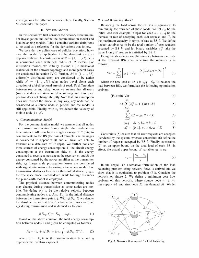
In the sequel, an alternative formulation of the loadbalancing problem using network flows is derived and weshow that it is equivalent to problem (P1). Consider thenetwork on figure 2. We define a minimum cost flowproblem on this network, where source node m ∈ Mhas supply +1 and sink node K has demand M . We let
K
1
k
C
...
y1K1
y1K
ykK1
ykKuk
yCK1
yCK
.
.
.
...
m
M
1
.
.
.
.
.
.
.
.
.
.
.
.
zkm
z11
zCM
u1
uC
+1
+1
+1
-M
Fig. 2: Network flow model for load balancing.
4
TABLE I: Parameter and Variable Definitions
Notation Definition Notation DefinitionC set of BSs indexed 1 to C Uk max capacity in terms of rate at BS kM set of static users indexed 1 to M q Minimum data traffic per requestN set of relay nodes indexed 1 to N yk Volume of user requests accepted at kF Message size (bits) zmk Flow variable for user m on cell kB Data rate (bps) ynkK Flow variable for cell k to sink K for request net Circuit energy consumption at the transmitter uk upper bound of variables yker Circuit energy consumption at the receiver xij Flow variable between nodes i and jed Energy consumption of the transmitters power amplifier T Time horizondbrake Threshold distance for change in the propagation losses model G = G(V, L); graph on space-time networkvj Velocity of node j Vp set of (i, a), where i ∈ N at time epoch avij Relative velocity between nodes i and j BSC super sink node for graph G on space-time networkDij Distance between nodes i and j V = {M, Vp, C, BSC}τ = F/B; Communication duration b(i) supply and demand on nodes in Gη Pathloss exponent λ weighting parameter between energy and delaySk Data traffic load of cell k γ weighting parameter between load balancing andfij total energy consumption between nodes i and j communication cost
variables zmk denote the flow of the arc from each sourcenode m to node k and we assume that they have capacityone and cost zero. Since the available capacity of each BSk is uk, we introduce uk arcs of capacity one from BS kto sink node K. We denote the flow of these arcs by ynkKwhere k = 1, . . . , C and n = 1, . . . , uk. The cost on linkynkK defined in equation (10) below reflects the increase inutilization of accepting the nth request over BS k and thusprovides a cost incentive for load balancing.
wk(n) = q Sk + n q2 (10)
Based on the above definitions, the minimum cost flowformulation of the above network is:
Constraints (12), (13) and (14) are the flow conservationconstraints for the source nodes m ∈ M, basestationsk = 1, . . . , C and the sink node K, respectively. Thecapacity constraints for the flow variables are given by(15) and (16) and since each request is services by asingle basestation, the integrality of these flows is a naturalassumption. However, the integrality constraints can berelaxed while guaranteing integer optimal solutions forproblem (P2).
Proposition 1: The linear programming relaxation ofproblem (P2) guarantees to give integer optimal solutions.
Proof: Min-cost flow formulations with integer sup-ply/demand and link capacities (as is the case here), haveinteger optimal solutions according to the integrality prin-ciple [19].
Furthermore, we have:Proposition 2: Problem (P1) is equivalent to problem
(P2).The proof can be found in appendix A. Importantly,given that the two problems are equivalent, then the loadbalancing problem can be solved using efficient linearprogramming algorithms,[19]. Noticeably, the derivationsabove have been based on the fact that each request imposesan equal increase in utilization in the system. Problem (P2)can be extended to include the alternative case where eachuser request imposes varying utilization requirements asshown in appendix B.
III. MATHEMATICAL MODEL
In this section we define a space-time network and for-mulate a linear program on this network that trades off load-balancing and communication costs of energy consumptionand delay.
A. Space-Time Network
To capture the dynamics of the network over consecutivetime epochs, we take snapshots of the changing networktopology at τ = F
B consecutive units of time over thehorizon T . In this way a time expanded network is formedwhere the position of all mobile nodes is described by thecoordinate (i, a) indicating the position of node i ∈ Nat the ath time epoch. Clearly, for all static nodes, thetime coordinate is redundant and thus their positions can beuniquely identified by the node index i. Illustratively, figure3 shows the time expanded network for a single user, twoBSs and four mobile relay nodes at three consecutive timeintervals. At time epoch 0 the current position of all nodesin the network is shown. Also a mobile node i ∈ N atthe first time epoch is index as (i, 1) while for the secondtime epoch is (i, 2) and so on. Set Vp contains all space-time network nodes of the form (i, a), where i ∈ N at theath time epoch. Future node positions can be generated bymobility prediction models to assess the network conditionsat different scenarios. It is important to note at this stagethat we do not require accurate mobility predictions for theproposed scheme to operate efficiently. In fact, we only
5
need to know the candidate serving BSs of a node and arough estimate of its location for each time epoch.
M VP C
UT1 BS2
(VR1,1) (VR2,1) (VR3,1) (VR4,1)
Timeepoch
2τ
3τ
τ
(VR1,0) (VR2,0) (VR3,0) (VR4,0)
Space
0
(VR1,2) (VR2,2) (VR3,2) (VR4,2)
(VR1,3) (VR2,3) (VR3,3) (VR4,3)
BS1
Fig. 3: Illustration of an instance of the space-time networkunder consideration. Future mobile node positions are replicatedat consecutive time epochs to generate a static network over time.
B. Graph on the Space-Time Network
On the space-time network described in the previoussubsection, we define the graph G = (V, L) where V ={M, Vp, C, BSC} is the set of nodes and L is the set oflinks, where we introduce node BSC (denoted by K) asa super sink node for all user requests. Node BSC can beconsidered as a physical entity (as is the case with currentcellular deployments that have a radio network controller)or a virtual node acting as a load aggregator. Further,the links in L are subdivided into three distinct subsetsdescribed as follows:L1 : Set of links where transmission between a
transceiver pair takes place.L2 : Set of links where no transmission occurs and in-
formation is physically propagated by mobile nodes.L3 : No information travels on these links. They are
dummy links that connect all BSs to the super sinknode BSC to ensure load balancing.
The L1 links are of the form i 7→ j, i ∈ M ∪ Vp, j ∈Vp ∪ C, where transmission of a single message occursbetween nodes i and j. For example, links UT1 7→ BS1,UT1 7→ (V R2, 2), (V R2, 1) 7→ (V R3, 2) and (V R3, 3) 7→BS2 shown in figure 4 are all L1 links. Notice that nodereplication on the space-time network is done every τ unitsof time. Therefore, for all communication links (i.e. linksin L1) a single message can be transmitted at consecutivetime instances. The delay in communication for links in L1
can vary with respect to the type of L1 link. There are fourtypes of L1 links shown below with their delays:
Case 1 : UTm 7→ BSk delay τ2 : UTm 7→ (V Rn, a) delay aτ3 : (V Rn, a) 7→ (V Rl, a+ 1) delay τ4 : (V Rn, a) 7→ BSk delay τ
(17)
where m ∈ M, k ∈ C, n, l ∈ N and a ∈ T . The first caseis simply the traditional direct communication and the delayis merely the communication time τ . For example, the firstcase is link UT1 7→ BS1 as shown in figure 4. In the secondcase, the message leaves the user at time 0 and arrives at
time epoch a; initially the user for the first a − 1 timeepochs is buffering the message while waiting for a mobilenode to approach and in the last time epoch is transmitsthe message. So the total delay is aτ . An example of thisin figure 4 is link UT1 7→ (V R2, 2) where the messageis buffered for the first time epoch and transmitted in thesecond time epoch. The third case represents transmissionbetween two mobile nodes and incurs delay τ . In figure 4this case is represented by link (V R2, 1) 7→ (V R3, 2). Thefourth case represents transmission from a mobile node toa base station as shown by link (V R3, 2) 7→ BS2 in figure4.
Links in L2 is denoted as follows, L2 ={(i, a) 7→ (i, a+ 1) : ∀(i, a), (i, a+ 1) ∈ Vp} where amobile node carries messages from one time period to thenext without any transmission taking place. For example infigure 4, (V R2, 1) 7→ (V R2, 2) and (V R3, 2) 7→ (V R3, 3)are two examples of L2.
M VP C BSC
Link in L2Link in L1 Link in L3
UT1 BS2
(VR1,1) (VR2,1) (VR3,1) (VR4,1)
Time
Space
(VR1,2) (VR2,2) (VR3,2) (VR4,2)
(VR1,3) (VR2,3) (VR3,3) (VR4,3)
BS1
BSC
Fig. 4: The figure illustrates a connected graph for the space-timenetwork under consideration. Selectively a number of links areshown.
Links in L3 are dummy links that we place betweenthe base stations and the sink node K in order to achieveload balancing. Since a BS can accept at most uk requests,similar to the network of problem (P2) (figure 2), we placemultiple arcs between BS k and sink node K each indexedby n = 1, . . . , uk of increasing convex cost to promote loadbalancing as in the problem P2. Therefore, link (kKn) ∈L3, k ∈ C, n = 1, . . . , uk identifies the nth link emanatingfrom BS k ∈ C and ending at the BSC. The cost on theselinks expresses the increase in utilization of accepting userrequests through an arbitrary BS. Therefore, the functionwk(n) as defined by equation (10) determines the cost ofaccepting the nth message through BS k.
We define the flow variable xij for links in L1 ∪L2 andflow variable ynkK for links in L3. Further, for links in L3
the flow should be kept binary to indicate the accept/rejectdecision of each request. It also accounts for the increasein load by an arbitrary BS when accepting a user request asdescribed in section II-B. On the other hand, mobile nodescan buffer an arbitrary number of messages while in transit.Therefore, the capacity for all links in L1 is uij = 1 andfor links in L2 we set it to the maximum possible, which isuij = M , since there are M users with one message each.In addition, the capacity for links in L3 is 1 unit flow asdetailed in section II-B. We define the supply and demand
6
for all nodes i ∈ V as follows:
b(i) =
+1 i ∈ M−M i = K0 otherwise
(18)
C. Link costs
The energy consumed in transmission of a unit flow forlinks in L1 and L2, is given as follows:
E(i 7→ j) =
{fij for i 7→ j ∈ L1
0 for i 7→ j ∈ L2,(19)
where fij is defined in section II-A. Note that in equation(2) the energy consumed in transmission is correct only fora unit flow as it is not linear to the number of flows send.However, for the multiplicative cost xijfij on a link in L1
as expressed by equation (19) it gives the correct cost as itcan attain only binary values.
The delay per unit flow for all links in L1 ∪ L2, usingj = (k, a+ 1), is as follows:
Φ(i 7→ j) =
{τ for i 7→ j ∈ L1 ∪ L2, i ∈ Mτ(a+ 1) for i 7→ j ∈ L1, i ∈ M,
(20)where for link i 7→ j ∈ L1, i ∈ M, the user postpones
transmission for a time periods before transmitting. Thetotal communication cost is thus defined as a weighted sumof the communication energy consumption and the delayincurred while traversing the link and is defined as follows,cij = E(i 7→ j) + λΦ(i 7→ j), i 7→ j ∈ L1 ∪ L2 whereλ is the weighting parameter for the two quantities. Notethat for hard deadline constraints, node replication can berestricted to a finite horizon T that allows for the maximumdelay tolerance of the service considered. In the latter case,the model is still valid, however the cost of L1 links issimply the energy consumption as expressed in equation(19), while for the L2 links the traversal cost is zero.
For links in L3, both the energy consumption and com-munication delay are assumed to be negligible.
D. Mathematical Programming Formulation
The space-time network model derived in the previoussection generates all feasible paths from the source nodesto the BSC through the available BSs. Clearly, decisionsneed to be made on the best forwarding nodes that couldpotentially forward messages and the time at which thesenodes need to forward data. In this section, we formulatethe joint routing and scheduling problem to generate theoptimal decision policies for message forwarding. We areinterested in finding forwarding paths that minimize theload imbalance in the system and at the same time reducingthe communication cost of the forwarding paths. The fol-lowing linear integer mathematical program is formulatedwhere the weights between the competitive parameters ofload balancing, communication energy consumption andmessage delivery delay can be set using parameters λ and γ.
These parameters can be weighted accordingly dependingon network operation preferences.
(P3) minimize∑
i 7→j∈L1∪L2
cijxij + γ∑
(kKn)∈L3
wk(n)ynkK (21)
s.t.∑
j:i 7→j∈L1
xij ≤ 1 ∀ i, i ∈ Vp (22)∑j:j 7→i∈L1
xji ≤ 1 ∀ i, i ∈ Vp (23)∑j:i 7→j∈L1∪L2
xij −∑
j:j 7→i∈L1∪L2
xji = b(i) ∀ i, i ∈ M∪ Vp
(24)∑n:(kKn)∈L3
ynkK −∑
j:j 7→k∈L1
xjk = b(k) ∀ k, k ∈ C (25)
−∑
n:(kKn)∈L3
ynkK = b(K) (26)
0 ≤ xij ≤ uij , xij ∈ Z, ynkK ∈ {0, 1} (27)
The objective function of problem (P3) minimizes theweighted sum cost of load imbalance and communicationcost in the multi-cell network topology. Constraint equa-tions (22-23) restrict all relay nodes to transmit and receivefrom a single other node at any one time. Constraints (24-26) are the flow conservation equations guaranteeing thegeneration of the end-to-end paths. Equations (27) are thecapacity and integrality constraints on the flow variables.Integrality is a natural assumption as all information mes-sages are considered to be independent units that can notbe split.
Due to the integer variables the mathematical programformulated by equations (21-27) is in general hard to solve.However, it can be shown that the linear programmingrelaxation of problem (P3) guarantees to give integer solu-tions. Therefore, the problem can be solved efficiently intime even for large instances.
Theorem 1: Let A[x; y] ≤ z be the matrix representationof constraints (22)-(27), ignoring integrality constraints.Then A is totally unimodular (TU).The proof is detailed in appendix C. It is well knownthat if A is TU and z is integer then the feasible regiondescribed by A[x; y] ≤ z has integer extreme points. Thus,we can relax the integrality constraints and still get integersolutions using linear programming (simplex method). Thismeans that we can solve the above mathematical programfor a large number of nodes in very short running times.
IV. NUMERICAL INVESTIGATIONS
Solving problem (P3) to optimality for different valuesof the weighting parameters, we study in this section thepossible performance gains of the proposed generalizedSCF scheme.
A. Simulation set-up
For the communication model we assume that all sourcenodes have a single message of size F = 4Mbit to
7
0 5 10 15 20 25 30 3510
2
10 1
100
MDD (sec)
NE
C
γ=0.1
γ=1
γ=10
γ=100
0 5 10 15 20 25 30 350
0.2
0.4
0.6
0.8
1
MDD (sec)L
B
γ=0.1
γ=1
γ=10
γ=100
(a)
0 5 10 15 20 25 30 3510
2
10 1
100
MDD (sec)
NE
C
γ=0.1
γ=1
γ=10
γ=100
0 5 10 15 20 25 30 350
0.2
0.4
0.6
0.8
1
MDD (sec)
LB
γ=0.1
γ=1
γ=10
γ=100
(b)
0 5 10 15 20 25 30 3510
2
10 1
100
MDD (sec)
NE
C
γ=0.1
γ=1
γ=10
γ=100
0 5 10 15 20 25 30 350
0.2
0.4
0.6
0.8
1
MDD (sec)
LB
γ=0.1
γ=1
γ=10
γ=100
(c)
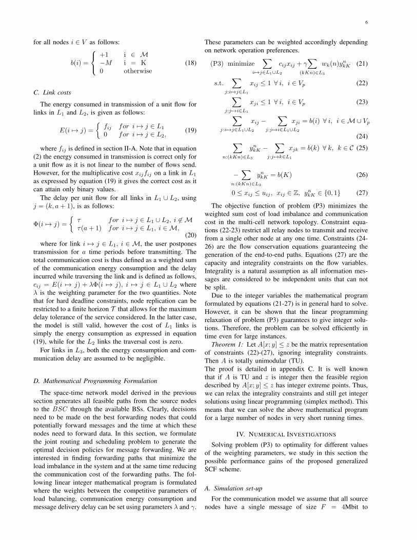
Fig. 5: Pareto curves for the optimal operating points of the proposed SCF relaying scheme, where γ is the tradeoff coefficient ofload balancing versus energy efficiency and delay: for a network topology of (a) 2 cells, 20 users and 40 relay nodes, (b) 3 cells, 30users and 60 relay nodes and (c) 4 cells, 40 users and 80 relay nodes.
0 5 10 15 200
0.2
0.4
0.6
0.8
1
MDD (sec)
NE
C
γ=0.1
γ=1
γ=10
γ=100
0 5 10 15 200
0.2
0.4
0.6
0.8
1
MDD (sec)
LB
γ=0.1
γ=1
γ=10
γ=100
(a)
0 5 10 15 200
0.2
0.4
0.6
0.8
1
MDD (sec)
NE
C
γ=0.1
γ=1
γ=10
γ=100
0 5 10 15 200
0.2
0.4
0.6
0.8
1
MDD (sec)
LB
γ=0.1
γ=1
γ=10
γ=100
(b)
0 5 10 15 200
0.2
0.4
0.6
0.8
1
MDD (sec)
NE
C
γ=0.1
γ=1
γ=10
γ=100
0 5 10 15 200
0.2
0.4
0.6
0.8
1
MDD (sec)
LB
γ=0.1
γ=1
γ=10
γ=100
(c)
Fig. 6: Performance evaluation of the basic multihop scheme: for a network topology of (a) 2 cells, 20 users and 40 relay nodes, (b)3 cells, 30 users and 60 relay nodes and (c) 4 cells, 40 users and 80 relay nodes.
0 5 10 15 20 25 30 35 40 45 5010
2
10 1
100
MDD (sec)
NE
C
γ=0.1
γ=1
γ=10
γ=100
0 5 10 15 20 25 30 35 40 45 50
0.4
0.5
0.6
0.7
0.8
0.9
1
MDD (sec)
LB
γ=0.1
γ=1
γ=10
γ=100
(a)
0 5 10 15 20 25 30 35 40 45 5010
2
10 1
100
MDD (sec)
NE
C
γ=0.1
γ=1
γ=10
γ=100
0 5 10 15 20 25 30 35 40 45 500
0.2
0.4
0.6
0.8
1
MDD (sec)
LB
γ=0.1
γ=1
γ=10
γ=100
(b)
0 5 10 15 20 25 30 35 40 45 5010
2
10 1
100
MDD (sec)
NE
C
γ=0.1
γ=1
γ=10
γ=100
0 5 10 15 20 25 30 35 40 45 500
0.2
0.4
0.6
0.8
1
MDD (sec)
LB
γ=0.1
γ=1
γ=10
γ=100
(c)
Fig. 7: Effect of the data request volume on the system performance gains: for a network topology of (a) 4 cells, 10 users and 80relay nodes, (b) 4 cells, 20 users and 80 relay nodes and (c) 4 cells, 30 users and 80 relay nodes.
0 5 10 15 20 250.1
0.2
0.3
0.4
0.5
0.6
0.7
0.8
0.9
1
MDD (sec)
NE
C
γ=0.1
γ=1
γ=10
γ=100
0 5 10 15 20 250
0.1
0.2
0.3
0.4
0.5
0.6
0.7
0.8
0.9
1
MDD (sec)
LB
γ=0.1
γ=1
γ=10
γ=100
(a)
0 5 10 15 20 25 3010
2
10 1
100
MDD (sec)
NE
C
γ=0.1
γ=1
γ=10
γ=100
0 5 10 15 20 25 300
0.2
0.4
0.6
0.8
1
MDD (sec)
LB
γ=0.1
γ=1
γ=10
γ=100
(b)
0 5 10 15 20 25 3010
2
10 1
100
MDD (sec)
NE
C
γ=0.1
γ=1
γ=10
γ=100
0 5 10 15 20 25 300
0.2
0.4
0.6
0.8
1
MDD (sec)
LB
γ=0.1
γ=1
γ=10
γ=100
(c)
Fig. 8: The effect of mobile node density on system performance: for (a) 4 cells, 40 users and 10 relay nodes, (b) 4 cells, 40 usersand 20 relay nodes and (c) 4 cells, 40 users and 30 relay nodes. Clearly for few relay nodes, the energy efficiency gains reduce asthe buffering queues grow larger. However, even for low relay node densities, load balancing gains are intact.
communicate to the wired network. All links transmit ata rate of B = 1Mbps and the radio wavelength is assumedto be ν = 0.126m. The antenna height for all nodes isassume to be hv = 1.5m, except for the BS where it ishb = 15m. Even though the device-to-device and device-to-BS communications possess very different propagationcharacteristics, we use the same channel model. A moredetailed channel model is not necessary since this work isconcerned with the energy efficiency gains that are achievedfrom communicating shorter distances.
The power consumed by the circuit electronics duringthe transmit/receive operations is Pc = 50mW, while thereceived power threshold for successful communicationis Pr = −52dBm1. From these values, the followingparameters can be deduced: The threshold distance forswitching between the two modes of propagation can beestimated as follow, dbrake = 4πh2
ν . The energy per bitconsumed by the power amplifier is ed(los) = Pr(4π)
2
Bν2
1This is similar to the average signal strength for an LTE receiver at10MHz channel bandwidth which is calculated in [20] to be -56.5dBm.
8
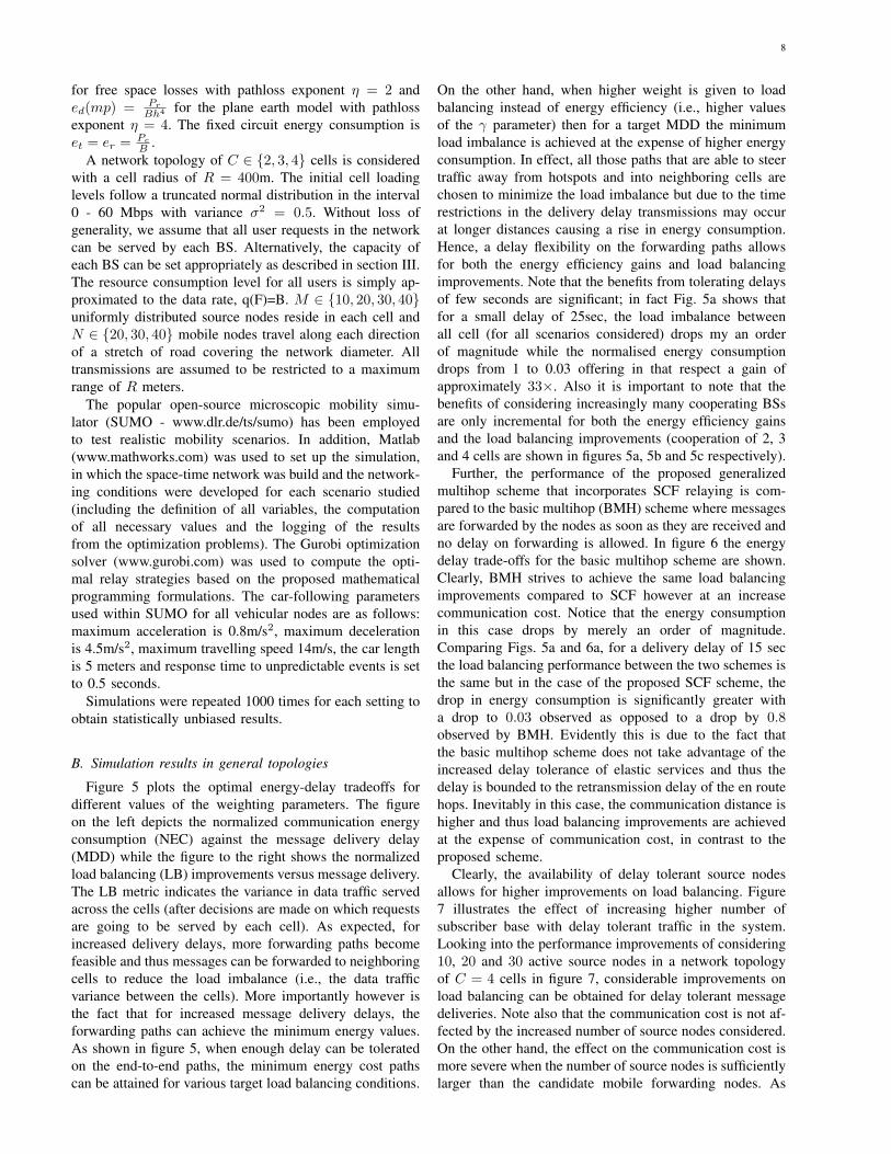
for free space losses with pathloss exponent η = 2 anded(mp) = Pr
Bh4 for the plane earth model with pathlossexponent η = 4. The fixed circuit energy consumption iset = er = Pc
B .A network topology of C ∈ {2, 3, 4} cells is considered
with a cell radius of R = 400m. The initial cell loadinglevels follow a truncated normal distribution in the interval0 - 60 Mbps with variance σ2 = 0.5. Without loss ofgenerality, we assume that all user requests in the networkcan be served by each BS. Alternatively, the capacity ofeach BS can be set appropriately as described in section III.The resource consumption level for all users is simply ap-proximated to the data rate, q(F)=B. M ∈ {10, 20, 30, 40}uniformly distributed source nodes reside in each cell andN ∈ {20, 30, 40} mobile nodes travel along each directionof a stretch of road covering the network diameter. Alltransmissions are assumed to be restricted to a maximumrange of R meters.
The popular open-source microscopic mobility simu-lator (SUMO - www.dlr.de/ts/sumo) has been employedto test realistic mobility scenarios. In addition, Matlab(www.mathworks.com) was used to set up the simulation,in which the space-time network was build and the network-ing conditions were developed for each scenario studied(including the definition of all variables, the computationof all necessary values and the logging of the resultsfrom the optimization problems). The Gurobi optimizationsolver (www.gurobi.com) was used to compute the opti-mal relay strategies based on the proposed mathematicalprogramming formulations. The car-following parametersused within SUMO for all vehicular nodes are as follows:maximum acceleration is 0.8m/s2, maximum decelerationis 4.5m/s2, maximum travelling speed 14m/s, the car lengthis 5 meters and response time to unpredictable events is setto 0.5 seconds.
Simulations were repeated 1000 times for each setting toobtain statistically unbiased results.
B. Simulation results in general topologies
Figure 5 plots the optimal energy-delay tradeoffs fordifferent values of the weighting parameters. The figureon the left depicts the normalized communication energyconsumption (NEC) against the message delivery delay(MDD) while the figure to the right shows the normalizedload balancing (LB) improvements versus message delivery.The LB metric indicates the variance in data traffic servedacross the cells (after decisions are made on which requestsare going to be served by each cell). As expected, forincreased delivery delays, more forwarding paths becomefeasible and thus messages can be forwarded to neighboringcells to reduce the load imbalance (i.e., the data trafficvariance between the cells). More importantly however isthe fact that for increased message delivery delays, theforwarding paths can achieve the minimum energy values.As shown in figure 5, when enough delay can be toleratedon the end-to-end paths, the minimum energy cost pathscan be attained for various target load balancing conditions.
On the other hand, when higher weight is given to loadbalancing instead of energy efficiency (i.e., higher valuesof the γ parameter) then for a target MDD the minimumload imbalance is achieved at the expense of higher energyconsumption. In effect, all those paths that are able to steertraffic away from hotspots and into neighboring cells arechosen to minimize the load imbalance but due to the timerestrictions in the delivery delay transmissions may occurat longer distances causing a rise in energy consumption.Hence, a delay flexibility on the forwarding paths allowsfor both the energy efficiency gains and load balancingimprovements. Note that the benefits from tolerating delaysof few seconds are significant; in fact Fig. 5a shows thatfor a small delay of 25sec, the load imbalance betweenall cell (for all scenarios considered) drops my an orderof magnitude while the normalised energy consumptiondrops from 1 to 0.03 offering in that respect a gain ofapproximately 33×. Also it is important to note that thebenefits of considering increasingly many cooperating BSsare only incremental for both the energy efficiency gainsand the load balancing improvements (cooperation of 2, 3and 4 cells are shown in figures 5a, 5b and 5c respectively).
Further, the performance of the proposed generalizedmultihop scheme that incorporates SCF relaying is com-pared to the basic multihop (BMH) scheme where messagesare forwarded by the nodes as soon as they are received andno delay on forwarding is allowed. In figure 6 the energydelay trade-offs for the basic multihop scheme are shown.Clearly, BMH strives to achieve the same load balancingimprovements compared to SCF however at an increasecommunication cost. Notice that the energy consumptionin this case drops by merely an order of magnitude.Comparing Figs. 5a and 6a, for a delivery delay of 15 secthe load balancing performance between the two schemes isthe same but in the case of the proposed SCF scheme, thedrop in energy consumption is significantly greater witha drop to 0.03 observed as opposed to a drop by 0.8observed by BMH. Evidently this is due to the fact thatthe basic multihop scheme does not take advantage of theincreased delay tolerance of elastic services and thus thedelay is bounded to the retransmission delay of the en routehops. Inevitably in this case, the communication distance ishigher and thus load balancing improvements are achievedat the expense of communication cost, in contrast to theproposed scheme.
Clearly, the availability of delay tolerant source nodesallows for higher improvements on load balancing. Figure7 illustrates the effect of increasing higher number ofsubscriber base with delay tolerant traffic in the system.Looking into the performance improvements of considering10, 20 and 30 active source nodes in a network topologyof C = 4 cells in figure 7, considerable improvements onload balancing can be obtained for delay tolerant messagedeliveries. Note also that the communication cost is not af-fected by the increased number of source nodes considered.On the other hand, the effect on the communication cost ismore severe when the number of source nodes is sufficientlylarger than the candidate mobile forwarding nodes. As
9
seen in figure 8, for a fixed number of source nodes,the availability of mobile relay nodes considerably affectsthe communication cost. This is expected as the mobilenodes receive messages from more source nodes which inturn transmit over longer distances when their queues havehigher loads. As the number of candidate forwarding nodesincreases however, there are more forwarding possibilitiesand the load is more evenly distributed across the nodes.Importantly though, is the fact that even for instances whenfew mobile nodes exist the load balancing improvementsare not deteriorated. This is so since mobile nodes actas message ferries; collecting and delivering delay tolerantmessages across adjacent cells.
Unfortunately, there are no general rules for choosing thedata routes since they change according to the many factorsmost important of which are the data traffic load of eachcell, the delay tolerance of the application, the opportunitiesfor SCF relaying provided by vehicle traffic routes andavailable vehicles. That is why we use the optimal solutionof an optimisation problem, which can tackle realistic sizenetworks in tractable computational times.
C. Simulation results in realistic topologies
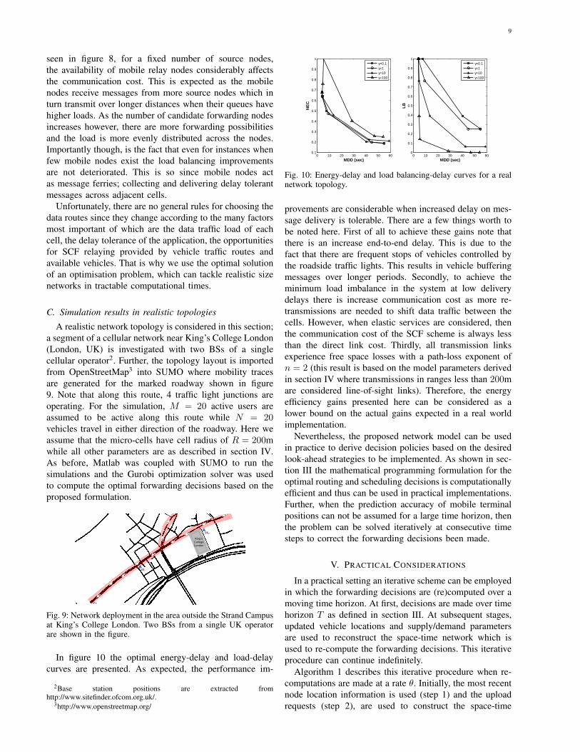
A realistic network topology is considered in this section;a segment of a cellular network near King’s College London(London, UK) is investigated with two BSs of a singlecellular operator2. Further, the topology layout is importedfrom OpenStreetMap3 into SUMO where mobility tracesare generated for the marked roadway shown in figure9. Note that along this route, 4 traffic light junctions areoperating. For the simulation, M = 20 active users areassumed to be active along this route while N = 20vehicles travel in either direction of the roadway. Here weassume that the micro-cells have cell radius of R = 200mwhile all other parameters are as described in section IV.As before, Matlab was coupled with SUMO to run thesimulations and the Gurobi optimization solver was usedto compute the optimal forwarding decisions based on theproposed formulation.
BS1
King’s
College
London
BS2
Fig. 9: Network deployment in the area outside the Strand Campusat King’s College London. Two BSs from a single UK operatorare shown in the figure.
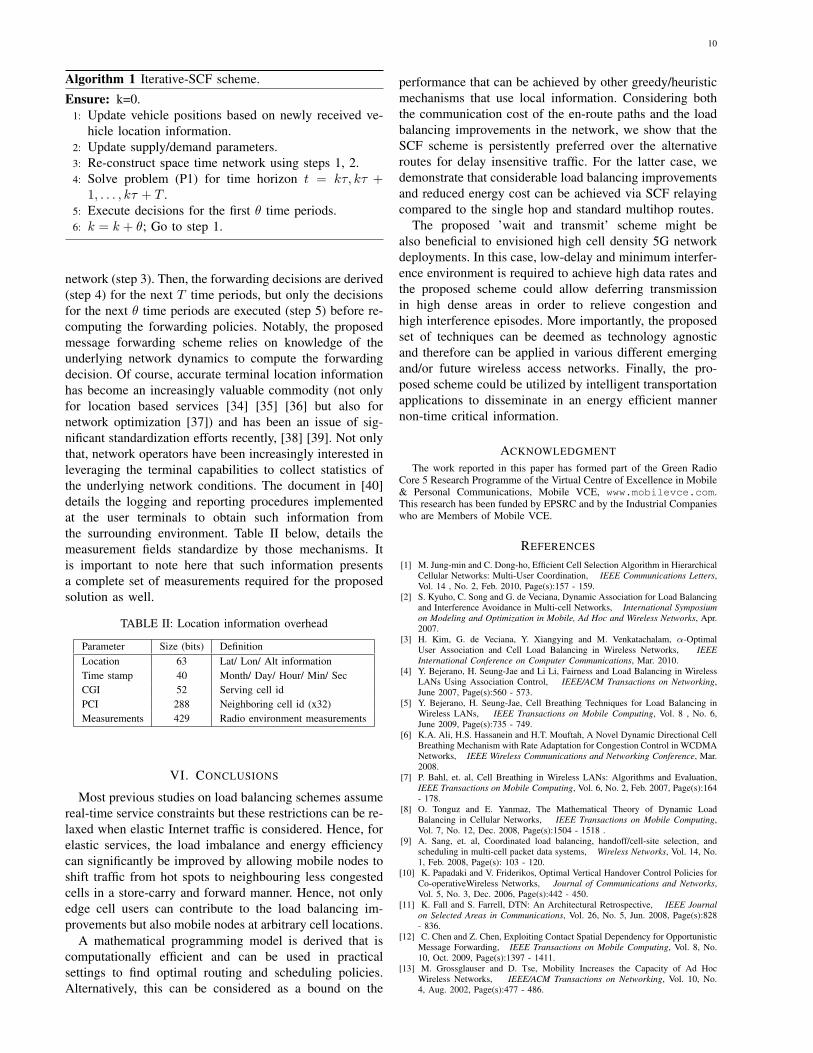
In figure 10 the optimal energy-delay and load-delaycurves are presented. As expected, the performance im-
2Base station positions are extracted fromhttp://www.sitefinder.ofcom.org.uk/.
3http://www.openstreetmap.org/
0 10 20 30 40 50 600.1
0.2
0.3
0.4
0.5
0.6
0.7
0.8
0.9
1
MDD (sec)
NE
C
γ=0.1γ=1γ=10γ=100
0 10 20 30 40 50 600
0.1
0.2
0.3
0.4
0.5
0.6
0.7
0.8
0.9
1
MDD (sec)
LB
γ=0.1γ=1γ=10γ=100
Fig. 10: Energy-delay and load balancing-delay curves for a realnetwork topology.
provements are considerable when increased delay on mes-sage delivery is tolerable. There are a few things worth tobe noted here. First of all to achieve these gains note thatthere is an increase end-to-end delay. This is due to thefact that there are frequent stops of vehicles controlled bythe roadside traffic lights. This results in vehicle bufferingmessages over longer periods. Secondly, to achieve theminimum load imbalance in the system at low deliverydelays there is increase communication cost as more re-transmissions are needed to shift data traffic between thecells. However, when elastic services are considered, thenthe communication cost of the SCF scheme is always lessthan the direct link cost. Thirdly, all transmission linksexperience free space losses with a path-loss exponent ofn = 2 (this result is based on the model parameters derivedin section IV where transmissions in ranges less than 200mare considered line-of-sight links). Therefore, the energyefficiency gains presented here can be considered as alower bound on the actual gains expected in a real worldimplementation.
Nevertheless, the proposed network model can be usedin practice to derive decision policies based on the desiredlook-ahead strategies to be implemented. As shown in sec-tion III the mathematical programming formulation for theoptimal routing and scheduling decisions is computationallyefficient and thus can be used in practical implementations.Further, when the prediction accuracy of mobile terminalpositions can not be assumed for a large time horizon, thenthe problem can be solved iteratively at consecutive timesteps to correct the forwarding decisions been made.
V. PRACTICAL CONSIDERATIONS
In a practical setting an iterative scheme can be employedin which the forwarding decisions are (re)computed over amoving time horizon. At first, decisions are made over timehorizon T as defined in section III. At subsequent stages,updated vehicle locations and supply/demand parametersare used to reconstruct the space-time network which isused to re-compute the forwarding decisions. This iterativeprocedure can continue indefinitely.
Algorithm 1 describes this iterative procedure when re-computations are made at a rate θ. Initially, the most recentnode location information is used (step 1) and the uploadrequests (step 2), are used to construct the space-time
10
Algorithm 1 Iterative-SCF scheme.
Ensure: k=0.1: Update vehicle positions based on newly received ve-
hicle location information.2: Update supply/demand parameters.3: Re-construct space time network using steps 1, 2.4: Solve problem (P1) for time horizon t = kτ, kτ +
1, . . . , kτ + T .5: Execute decisions for the first θ time periods.6: k = k + θ; Go to step 1.
network (step 3). Then, the forwarding decisions are derived(step 4) for the next T time periods, but only the decisionsfor the next θ time periods are executed (step 5) before re-computing the forwarding policies. Notably, the proposedmessage forwarding scheme relies on knowledge of theunderlying network dynamics to compute the forwardingdecision. Of course, accurate terminal location informationhas become an increasingly valuable commodity (not onlyfor location based services [34] [35] [36] but also fornetwork optimization [37]) and has been an issue of sig-nificant standardization efforts recently, [38] [39]. Not onlythat, network operators have been increasingly interested inleveraging the terminal capabilities to collect statistics ofthe underlying network conditions. The document in [40]details the logging and reporting procedures implementedat the user terminals to obtain such information fromthe surrounding environment. Table II below, details themeasurement fields standardize by those mechanisms. Itis important to note here that such information presentsa complete set of measurements required for the proposedsolution as well.
TABLE II: Location information overhead
Parameter Size (bits) DefinitionLocation 63 Lat/ Lon/ Alt informationTime stamp 40 Month/ Day/ Hour/ Min/ SecCGI 52 Serving cell idPCI 288 Neighboring cell id (x32)Measurements 429 Radio environment measurements
VI. CONCLUSIONS
Most previous studies on load balancing schemes assumereal-time service constraints but these restrictions can be re-laxed when elastic Internet traffic is considered. Hence, forelastic services, the load imbalance and energy efficiencycan significantly be improved by allowing mobile nodes toshift traffic from hot spots to neighbouring less congestedcells in a store-carry and forward manner. Hence, not onlyedge cell users can contribute to the load balancing im-provements but also mobile nodes at arbitrary cell locations.
A mathematical programming model is derived that iscomputationally efficient and can be used in practicalsettings to find optimal routing and scheduling policies.Alternatively, this can be considered as a bound on the
performance that can be achieved by other greedy/heuristicmechanisms that use local information. Considering boththe communication cost of the en-route paths and the loadbalancing improvements in the network, we show that theSCF scheme is persistently preferred over the alternativeroutes for delay insensitive traffic. For the latter case, wedemonstrate that considerable load balancing improvementsand reduced energy cost can be achieved via SCF relayingcompared to the single hop and standard multihop routes.
The proposed ’wait and transmit’ scheme might bealso beneficial to envisioned high cell density 5G networkdeployments. In this case, low-delay and minimum interfer-ence environment is required to achieve high data rates andthe proposed scheme could allow deferring transmissionin high dense areas in order to relieve congestion andhigh interference episodes. More importantly, the proposedset of techniques can be deemed as technology agnosticand therefore can be applied in various different emergingand/or future wireless access networks. Finally, the pro-posed scheme could be utilized by intelligent transportationapplications to disseminate in an energy efficient mannernon-time critical information.
ACKNOWLEDGMENT
The work reported in this paper has formed part of the Green RadioCore 5 Research Programme of the Virtual Centre of Excellence in Mobile& Personal Communications, Mobile VCE, www.mobilevce.com.This research has been funded by EPSRC and by the Industrial Companieswho are Members of Mobile VCE.
REFERENCES
[1] M. Jung-min and C. Dong-ho, Efficient Cell Selection Algorithm in HierarchicalCellular Networks: Multi-User Coordination, IEEE Communications Letters,Vol. 14 , No. 2, Feb. 2010, Page(s):157 - 159.
[2] S. Kyuho, C. Song and G. de Veciana, Dynamic Association for Load Balancingand Interference Avoidance in Multi-cell Networks, International Symposiumon Modeling and Optimization in Mobile, Ad Hoc and Wireless Networks, Apr.2007.
[3] H. Kim, G. de Veciana, Y. Xiangying and M. Venkatachalam, α-OptimalUser Association and Cell Load Balancing in Wireless Networks, IEEEInternational Conference on Computer Communications, Mar. 2010.
[4] Y. Bejerano, H. Seung-Jae and Li Li, Fairness and Load Balancing in WirelessLANs Using Association Control, IEEE/ACM Transactions on Networking,June 2007, Page(s):560 - 573.
[5] Y. Bejerano, H. Seung-Jae, Cell Breathing Techniques for Load Balancing inWireless LANs, IEEE Transactions on Mobile Computing, Vol. 8 , No. 6,June 2009, Page(s):735 - 749.
[6] K.A. Ali, H.S. Hassanein and H.T. Mouftah, A Novel Dynamic Directional CellBreathing Mechanism with Rate Adaptation for Congestion Control in WCDMANetworks, IEEE Wireless Communications and Networking Conference, Mar.2008.
[7] P. Bahl, et. al, Cell Breathing in Wireless LANs: Algorithms and Evaluation,IEEE Transactions on Mobile Computing, Vol. 6, No. 2, Feb. 2007, Page(s):164- 178.
[8] O. Tonguz and E. Yanmaz, The Mathematical Theory of Dynamic LoadBalancing in Cellular Networks, IEEE Transactions on Mobile Computing,Vol. 7, No. 12, Dec. 2008, Page(s):1504 - 1518 .
[9] A. Sang, et. al, Coordinated load balancing, handoff/cell-site selection, andscheduling in multi-cell packet data systems, Wireless Networks, Vol. 14, No.1, Feb. 2008, Page(s): 103 - 120.
[10] K. Papadaki and V. Friderikos, Optimal Vertical Handover Control Policies forCo-operativeWireless Networks, Journal of Communications and Networks,Vol. 5, No. 3, Dec. 2006, Page(s):442 - 450.
[11] K. Fall and S. Farrell, DTN: An Architectural Retrospective, IEEE Journalon Selected Areas in Communications, Vol. 26, No. 5, Jun. 2008, Page(s):828- 836.
[12] C. Chen and Z. Chen, Exploiting Contact Spatial Dependency for OpportunisticMessage Forwarding, IEEE Transactions on Mobile Computing, Vol. 8, No.10, Oct. 2009, Page(s):1397 - 1411.
[13] M. Grossglauser and D. Tse, Mobility Increases the Capacity of Ad HocWireless Networks, IEEE/ACM Transactions on Networking, Vol. 10, No.4, Aug. 2002, Page(s):477 - 486.
11
[14] S.C. Borst, N. Hegde and A. Proutiere, Mobility-Driven Scheduling in WirelessNetworks, IEEE Conference on Computer Communications, Apr. 2009,Page(s):1260 - 1268.
[15] S. Chakraborty, Y. Dong, D. Yau and J. Lui, On the Effectiveness of MovementPrediction to Reduce Energy Consumption in Wireless Communication, IEEETransactions on Mobile Computing, Vol. 5, No. 2, Feb. 2006, Page(s):157 -169.
[16] Y. Dong, WK. Hon, D. Yau and JC. Chin, Distance Reduction in MobileWireless Communication: Lower Bound Analysis and Practical Attainment,IEEE Transactions on Mobile Computing, Vol. 8, No. 2, Feb. 2009, Page(s):276- 287.
[17] A. Venkateswaran, V. Sarangan, T. La Porta and R. Acharya, A Mobility-Prediction-Based Relay Deployment Framework for Conserving Power inMANETs , IEEE Transactions on Mobile Computing, Vol. 8, No. 6, Jun.2009, Page(s):750 - 765.
[18] C. Grote, IoT on the Move: The Ultimate Driving Machine as the UltimateMobile Thing, IEEE International Conference on Pervasive Computing andCommunications, 2014.
[20] H. Holma and A. Toskala, LTE for UMTS - OFDMA and SC-FDMA BasedRadio Access, John Wiley & Sons, Ltd, 1st. Ed., 2009, Page(s):341.
[21] P. Kolios, V. Friderikos and K. Papadaki, Energy-aware mobile video trans-mission utilizing mobility, IEEE Network, Vol. 27, No. 2, Mar. 2013.
[22] G. Alyfantis, S. Hadjiefthymiades and L. Merakos, Exploiting user locationfor load balancing WLANs and improving wireless QoS, ACM Transactionson Autonomous and Adaptive Systems, Vol. 4, No. 2, May 2009.
[23] A. Balachandran, P. Bahl and G. M. Voelker, Hot-Spot Congestion Reliefin Public-Area Wireless Networks, IEEE Workshop on Mobile ComputingSystems and Applications, Aug. 2002.
[24] G. Fettweis and E. Zimmermann, ICT Energy Consumption - Trends andChallenges, International Symposium on Wireless Personal Multimedia Com-munications, Sept. 2008.
[25] S. Vadgama, Trends in Green Wireless Access, Fujitsu Sci. Tech. J., Vol: 45,No: 4, Oct. 2009, Page(s):404 - 408.
[26] Cisco, Cisco Visual Networking Index: Global Mobile Data Traffic ForecastUpdate, 2012 - 2017, Cisco white paper, Feb. 2013.
[27] P. Kolios, V. Friderikos and K.Papadaki, Energy Efficient Relaying via Store-Carry and Forward within the Cell, IEEE Transactions on Mobile Computing,Nov. 2012.
[28] NGMN Alliance, Next Generation Mobile Networks 5G White Paper V1.0,NGMN 5G Initiative, February 2015
[29] 3GPP RWS-120010 WS Docomo, Requirement, candidate Solutions andTechnology Roadmap for LTE Rel-12 onward, 3GPP Workshop on Release12 and on-wards Ljubljana, Slovenia, June 11-12, 2012
[30] 5G Radio Access: Requirements, Concepts and Technologies, Docomo 5GWhite Paper, July 2014
[31] L. Chen, L. Libman, and J. Leneutre, Conflicts and incentives in wireless coop-erative relaying: A distributed market pricing framework. IEEE Transactions onParallel and Distributed Systems, Vol. 22, No. 5, May 2011, Page(s): 758-772.
[32] C. Comaniciu, B.M. Narayan, H. Vincent Poor, and J.M. Gorce, An AuctioningMechanism for Green Radio, Journal of Communications and Networks, Vol.12, No. 2, April 2010, Page(s):114 - 121.
[33] A. Schrijver, Theory of Linear and Integer Programming, Wiley Press, April1998.
[34] S. Wang, J Min and B. Yi, Location Based Services for Mobiles: Technologiesand Standards, IEEE International Conference on Communications, Tutorial,May 2008.
[35] Google, The Mobile Movement: Understanding Smartphone Users,Google/IPSOS OTX MediaCT, Apr. 2011, www.google.com/think/insights.
[36] C. Botezatu and C. Barca, Intelligent vehicle safety-eCALL, e-Society, 2008.[37] T. Jansen, et al. Handover parameter optimization in LTE self-organizing
networks, IEEE Vehicular Technology Conference, Sept. 2009.[38] Y. Zhao, Standardization of Mobile Phone Positioning for 3G Systems, IEEE
Radio Access Network (E-UTRAN); Stage 2 functional specification of userequipment positioning in E-UTRAN, ETSI Technical Specification 136 305V9.0.0 Release 9, Oct. 2009.
[40] 3GPP, Technical Specification Group Radio Access Network Study on Min-imization of drive-tests in Next Generation Networks, 3GPP, TR 36.805v9.0.0, Dec. 2009.
APPENDIX
Appendix A
Load variance minimization: proof of proposition 2:Proof:
Concerning the objective function of problem (P1): Ex-panding equation (3) and using
∑Ck=1 yk = M , which
ensures that all user requests are accepted by the network,results in the following expression:
Var =C∑
k=1
(ykq)2 + 2
C∑k=1
(ykq) Sk + f(M,Sk, q) (28)
where the function f(M,Sk, q) does not depend on yk.Concerning the objective of problem (P2): Let vk =∑uk
n=1 ynkK be the number of requests satisfied by BS k.
The weights of decision variables ynkK in the objective forn = 1, . . . , uk satisfy wk(1) < . . . < wk(uk) and since weare minimizing, the optimal solution will choose the firstvk arcs. Thus we can write the objective of (P2) as follows:
C∑k=1
[vk∑n=1
(wk(n))
]=
C∑k=1
[vkqSk +
vk[vk + 1]q2
2
](29)
As a sum of its terms, equation (29) can be expressed asfollows:
C∑k=1
vkqSk +1
2
C∑k=1
[vkq]2 +
q2
2
C∑k=1
vk (30)
Since∑C
m=1 vk = M , then the last term in (30) is aconstant.
From (28), we can see that (30) is equivalent to Var2 .
Thus, the objective functions of problems (P1) and (P2)are equivalent.
Consider now the constraints in both (P1) and (P2). Itis straightforward to see that vk =
∑uk
m=1 ymkK in (P2) is
identical to yk in (P1). In effect, constraint (5) is identicalto (11), (6) is identical to (12), (7) is identical to (15) and(8) is identical to (14). Moreover, constraint (13) in (P2) isredundant and thus the two problems are equivalent.
Appendix B
Load balancing model extensions: The derivation ofthe load balancing model in section II-B considered thecase when all user requests consumed the same amountof resources by all infrastructure nodes. Here, we extendthat model to consider the case when user requests requiredifferent resource consumption levels. For the model struc-ture and the formulation hereafter consider the illustrationin figure 2. Let qm be the resource consumption level ofthe mth request. Then, the greatest common divisor of allrequest levels qm, m ∈ M is q. Given q, the capacity ofall links m 7→ k, ∀m ∈ M, ∀k ∈ C can be expressed asumk = qm
q . Further, here we have two types of variables,the flow variables z, y as shown in the diagram in figure 2and binary variables δ indicating the acceptance (or not) ofa request through a specific infrastructure node.
As before the flow variable from a source node mto BS k is zmk and the cost of the flow is assumed tobe zero. Further, the remaining capacity of the BSs isdecomposed into the q parts as defined above and thus thetotal number of links emanating from k and ending at Kis ∆k = min(
∑Mm=1
qmq ,⌊Uk−Sk
q
⌋) (according to figure 2,
uk = ∆k). A flow variable flow yikK , i ∈ ∆k represent
12
the flow of the ith q fragment of user request send throughbasestation k. The cost function for the ith component ofa user request can be expressed as follows:
wk(i) = q Sk + i q2. (31)
In this case, the load balancing formulation can then bedescribed as follows.
minC∑
k=1
∆k∑i=1
wk(i)yikK (32)
s.t.C∑
k=1
qzmk = qm, ∀m ∈ M (33)
M∑m=1
zmk −∆k∑i=1
yikK = 0 ∀ k ∈ C (34)
−C∑
k=1
∆k∑i=1
qyikK = −M∑m
qm (35)
zmk = δmk umk , ∀ k ∈ C,m ∈ M (36)
C∑k=1
δmk = 1 ∀m ∈ M (37)
0 ≤ zmk ≤ umk , 0 ≤ yikK ≤ 1, δmk = {0, 1} (38)
The objective function (32) minimizes the load imbal-ance in the network. Constraints (33-35) are the flowconservation constraints. Constraints (36) ensure that thecomponents of each request are serviced by a single BS.Therefore, the flow of the mth user request is either 0 orumk . Constraints (37) ensure that each request is serviced
by a single BS. Equations (38) constraint the flow variablesand define the binary indicator variables.
Note that in this case the binary variables δmk areintroduced in the formulation that significantly increasethe computational complexity of the solution. However,as derived here, the problem formulation is valid for thegeneral case where arbitrary user flows are requested andthus optimal forwarding decisions can be made.
Appendix C
Total unimodularity: proof of theorem 1: Let matrix Cbe the node-arc incidence matrix for the flow conservationconstraints (24-26). Then the expressions {x, y ≥ 0 :C[x; y] = b} and {x, y ≥ 0 : C[x; y] ≤ b,−C[x; y] ≤ −b}are equivalent ways of describing these constraints. Further,let OUT and IN be the constraint matrices for the out-degree and in-degree constraints (equations (22) and (23),respectively), whose columns only correspond to links inL1. For the capacity constraints, expressed by equation (27)in problem (P3), only links in L1 and L3 have unity values.Thus the capacity constraint matrix for links in L1 andL3 is the identity matrix, I . Initially we ignore the non-negativity constraints and consider them later in the proof.We define A[x; y] ≤ z to be the matrix formed by theconstraint equations (22)-(27), ignoring non-negativity andintegrality constraints. Then A is characterized as follows:
L1︷︸︸︷ L3︷︸︸︷ L2︷︸︸︷A =
C−CI 0
OUT 0 0IN 0 0
(39)
We show that A is a network matrix and total unimod-ularity of network matrices is shown in [33]. A networkmatrix is defined as follows (further details can be foundin [33]):
Definition S is a network matrix, if there exists a di-rected graph Q = (Vq, E) and a directed spanning treeT = (Vq, E(T )) of Q, such that for each element e =(v, w) ∈ E \ E(T ) and e′ ∈ E(T ), S(e′, e) is defined asfollows:
S(e′, e)=
+1v-w path in T passes from e′ forwardly−1v-w path in T passes from e′ backwardly0 v-w path in T does not pass through e′
(40)
The rows of S correspond to edges of the tree T and thecolumns of S correspond to non-tree edges of Q. Further,each column of S that corresponds to a non-tree arc e =(v, w) traces the unique path from v to w on the tree T .
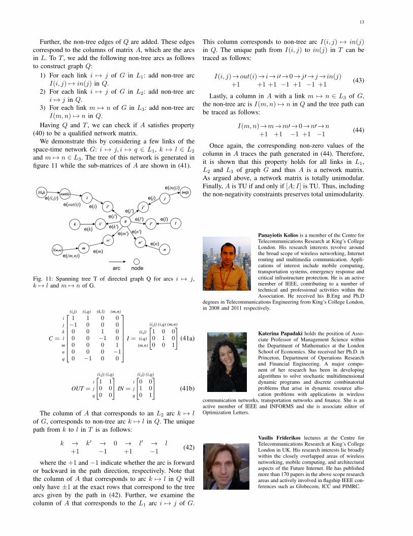
To show that A is a network matrix, a directed graph Qand a directed spanning tree T of Q are first generated. TreeT can be derived from the space-time network G = (V, L)and the constraint matrix A by tracing the following steps:
1) Add initial node 0.2) For every node in i ∈ V of the space-time network
add: nodes i, i′ to T and arcs e(i) = i 7→ i′ ande(i′) = 0 7→ i′.
3) For every L1 link i 7→ j of the space-time network:a) Add node out(i) and arc e(out(i)) = out(i) 7→
i, if not already available.b) Add node in(j) and arc e(in(i)) = j 7→ in(j),
if not already available.4) For every L1 link i 7→ j of the space-time network,
add node I(i, j) and arc e(i, j) = I(i, j) 7→ out(i).5) For every L3 link m 7→ n of the space-time network,
add node I(m,n) and arc e(m,n) = I(m,n) 7→ m.Note that the arcs of the tree T correspond to the rows
of A. For the rows of matrix C, which are the nodes of thespace-time network G, we add arcs e(i) = i 7→ i′ and forthe rows of −C we add arcs e(i′) = 0 7→ i′ (step 2). Therows of matrix I are the links L1∪L3 of G, and the rows ofmatrices OUT , IN are the nodes in Vp that have L1 linksincident to them. Corresponding to a link i 7→ j in L1: forthe rows in OUT we add arcs e(out(i)) = out(i) 7→ i to T ,for the rows in IN we add arcs e(in(i)) = j 7→ in(j) (step3), and for the rows in I we add arcs e(i, j) = I(i, j) 7→out(i), i 7→ j ∈ L1 and e(m,n) = I(m,n) 7→ m, m 7→n ∈ L3 (steps 4 and 5). In this way, the rows of matrix Aare mapped to arcs in tree T .
13
Further, the non-tree edges of Q are added. These edgescorrespond to the columns of matrix A, which are the arcsin L. To T , we add the following non-tree arcs as followsto construct graph Q:
1) For each link i 7→ j of G in L1: add non-tree arcI(i, j) 7→ in(j) in Q.
2) For each link i 7→ j of G in L2: add non-tree arci 7→ j in Q.
3) For each link m 7→ n of G in L3: add non-tree arcI(m,n) 7→ n in Q.
Having Q and T , we can check if A satisfies property(40) to be a qualified network matrix.
We demonstrate this by considering a few links of thespace-time network G: i 7→ j, i 7→ q ∈ L1, k 7→ l ∈ L2
and m 7→ n ∈ L3. The tree of this network is generated infigure 11 while the sub-matrices of A are shown in (41).
e((i,j))
e(out(i)) e(i)
e(i')e(j')
e(l')
e(k')e(k)
e(l)
e(in(j))
e(j)
arc node
I(i,j) out(i)i
i'
k k'0
l' l
j'
j
in(j)
e(m')
e(m)m
m'
e(n')
e(n)n'
nI(m,n)
e((m,n))
Fig. 11: Spanning tree T of directed graph Q for arcs i 7→ j,k 7→ l and m 7→ n of G.
The column of A that corresponds to an L2 arc k 7→ lof G, corresponds to non-tree arc k 7→ l in Q. The uniquepath from k to l in T is as follows:
k → k′ → 0 → l′ → l+1 −1 +1 −1
(42)
where the +1 and −1 indicate whether the arc is forwardor backward in the path direction, respectively. Note thatthe column of A that corresponds to arc k 7→ l in Q willonly have ±1 at the exact rows that correspond to the treearcs given by the path in (42). Further, we examine thecolumn of A that corresponds to the L1 arc i 7→ j of G.
This column corresponds to non-tree arc I(i, j) 7→ in(j)in Q. The unique path from I(i, j) to in(j) in T can betraced as follows:
Lastly, a column in A with a link m 7→ n ∈ L3 of G,the non-tree arc is I(m,n) 7→ n in Q and the tree path canbe traced as follows:
I(m,n)→m→m′→0→n′→n+1 +1 −1 +1 −1
(44)
Once again, the corresponding non-zero values of thecolumn in A traces the path generated in (44). Therefore,it is shown that this property holds for all links in L1,L2 and L3 of graph G and thus A is a network matrix.As argued above, a network matrix is totally unimodular.Finally, A is TU if and only if [A; I] is TU. Thus, includingthe non-negativity constraints preserves total unimodularity.
Panayiotis Kolios is a member of the Centre forTelecommunications Research at King’s CollegeLondon. His research interests revolve aroundthe broad scope of wireless networking, Internetrouting and multimedia communication. Appli-cations of interest include mobile computing,transportation systems, emergency response andcritical infrastructure protection. He is an activemember of IEEE, contributing to a number oftechnical and professional activities within theAssociation. He received his B.Eng and Ph.D
degrees in Telecommunications Engineering from King’s College London,in 2008 and 2011 respectively.
Katerina Papadaki holds the position of Asso-ciate Professor of Management Science withinthe Department of Mathematics at the LondonSchool of Economics. She received her Ph.D. inPrinceton, Department of Operations Researchand Financial Engineering. A major compo-nent of her research has been in developingalgorithms to solve stochastic multidimensionaldynamic programs and discrete combinatorialproblems that arise in dynamic resource allo-cation problems with applications in wireless
communication networks, transportation networks and finance. She is anactive member of IEEE and INFORMS and she is associate editor ofOptimization Letters.
Vasilis Friderikos lectures at the Centre forTelecommunications Research at King’s CollegeLondon in UK. His research interests lie broadlywithin the closely overlapped areas of wirelessnetworking, mobile computing, and architecturalaspects of the Future Internet. He has publishedmore than 170 papers in the above scope researchareas and actively involved in flagship IEEE con-ferences such as Globecom, ICC and PIMRC.