TESIS DOCTORAL

Panel Data Models with Long-Range Dependence

Autor:

Yunus Emre Ergemen

Director/es:

Prof. Carlos Velasco

DEPARTAMENTO/INSTITUTO DE

ECONOMIA

Getafe, 2015

( a entregar en la Oficina de Posgrado, una vez nombrado el Tribunal evaluador , para preparar el

documento para la defensa de la tesis)

TESIS DOCTORAL

PANEL DATA MODELS WITH LONG-RANGE DEPENDENCE

Autor: Yunus Emre Ergemen

Director/es: Prof. Carlos Velasco

Firma del Tribunal Calificador:

Firma

Presidente: Jesús Gonzalo Muñoz

Vocal: Javier Hualde

Secretario: Mª del Pilar Poncela Blanco

Calificación:

Getafe, de de 2015

Panel Data Models with Long-Range Dependence

Universidad Carlos III de Madrid

Yunus Emre Ergemen

08 May 2015

Abstract

This thesis comprises of three chapters that study panel data models with long-range dependence.

The first chapter is a coauthored paper with Prof. Carlos Velasco. We consider large N, T

panel data models with fixed effects, common factors allowing cross-section dependence, and

persistent data and shocks, which are assumed fractionally integrated. In a basic setup, the

main interest is on the fractional parameter of the idiosyncratic component, which is estimated

in first differences after factor removal by projection on the cross-section average. The pooled

conditional-sum-of-squares estimate is√NT consistent but the normal asymptotic distribution

might not be centered, requiring the time series dimension to grow faster than the cross-section size

for correction. Generalizing the basic setup to include covariates and heterogeneous parameters,

we propose individual and common-correlation estimates for the slope parameters, while error

memory parameters are estimated from regression residuals. The two parameter estimates are√T consistent and asymptotically normal and mutually uncorrelated, irrespective of possible

cointegration among idiosyncratic components. A study of small-sample performance and an

empirical application to realized volatility persistence are included.

The second chapter extends the first chapter. In this paper, a general dynamic panel data model

is considered that incorporates individual and interactive fixed effects and possibly correlated

innovations. The model accommodates general stationary or nonstationary long-range dependence

through interactive fixed effects and innovations, removing the necessity to perform a priori unit-

root or stationarity testing. Moreover, persistence in innovations and interactive fixed effects

allows for cointegration; innovations can also have vector-autoregressive dynamics; deterministic

trends can be nested. Estimations are performed using conditional-sum-of-squares criteria based

on projected series by which latent characteristics are proxied. Resulting estimates are consistent

and asymptotically normal at parametric rates. A simulation study provides reliability on the

estimation method. The method is then applied to the long-run relationship between debt and

GDP.

The third and final chapter of the thesis is a coauthored paper with Prof. Abderrahim

Taamouti. In this paper, a parametric portfolio policy function is considered that incorporates

common stock volatility dynamics to optimally determine portfolio weights. Reducing dimension

of the traditional portfolio selection problem significantly, only a number of policy parameters cor-

responding to first- and second-order characteristics are estimated based on a standard method-

of-moments technique. The method, allowing for the calculation of portfolio weight and return

1

statistics, is illustrated with an empirical application to 30 U.S. industries to study the economic

activity before and after the recent financial crisis.

2

Acknowledgements

First and foremost, I would like to thank my family who always supported me, and this thesis is

dedicated to them. Their support has always been incredible.

I wish to express my sincere gratitude to my supervisor Prof. Carlos Velasco, from whom

I learned a great deal, for treating me as a colleague rather than just a student, continuously

encouraging me to do better and always believing in me.

I am extremely grateful to Professors Jesus Gonzalo, Juan Jose Dolado and Abderrahim

Taamouti, who have always been very kind to lend a hand when I needed, for being encouraging

and supportive.

I want to place on record my sincere thanks to Professors Manuel Arellano, Yoosoon Chang,

Miguel Delgado, Niels Haldrup, Javier Hualde, Serena Ng, Bent Nielsen, Peter M. Robinson,

Enrique Sentana and the participants in CREATES Seminar 2015, RES Meeting 2015 and NBER-

NSF Time Series Conference 2014, the 67th Econometric Society European Meeting, CREATES

Symposium on Long Memory 2013, Robust Econometric Methods for Modeling Economic and

Financial Variables Conference 2012, UC3M Seminars, IIIt, IVt and Vt Workshop in Time Series

Econometrics for helpful comments and discussions that prompted improvements in parts of this

thesis.

I also would like to gratefully acknowledge financial support from the Spanish Plan Nacional

de I+D+I (ECO2012-31748), Spanish Ministerio de Ciencia e Innovacion grant ECO2010-19357

and Consolider-2010 that made it possible for me to attend conferences and meetings all over the

world.

Finally, I would like to thank (in no specific order) Anil Yildizparlak, Fabian Rinnen, Robert

Kirkby, Eleonora Garlandi, Lian Allub, Albert Riera, Marta Sanz, Marta Rekas, Pedro H.C.

Sant’anna, Nikolaos Tsakas, Xiaojun Song, Lovleen Kushwah, Victor Troster, Christos Mavridis,

Sebastian Panthofer, Mehdi Hamidisahneh, Federico Masera, Andres Garcia-Suaza and Marco

Serena for being super fun to hang out with at work, and I am very grateful to Nazli Aktakke,

Zeynep Ozkok, Tugba Taskiran, Ceren Genc, Giulia Bonnat, Matthias D’haene, Nicolas Garcia

Sanchez, Antoine Mairal, Edu Nogales Corrales, Paula Toledo Piza, Firat Akcal, Georgette Rio

Hewison, Andrzej Pioch, Anna Oldinger, Emily Wells, Christopher Kristiansen, Robbie Heim,

Jean-Francois Mercier, Alex Barrachina, Egemen Eren and Rutkay Ardogan for constantly re-

minding me that there is a life outside academia. Life would not have been the same without you

guys!

3

Contents

1 Estimation of Fractionally Integrated Panel Data Models with Fixed Effects

and Cross-Section Dependence (with Carlos Velasco) 6

1.1 Introduction . . . . . . . . . . . . . . . . . . . . . . . . . . . . . . . . . . . . . . . 1

1.2 The Basic Model . . . . . . . . . . . . . . . . . . . . . . . . . . . . . . . . . . . . 3

1.3 Parameter Estimation . . . . . . . . . . . . . . . . . . . . . . . . . . . . . . . . . 6

1.3.1 Estimation of a Heterogeneous Model . . . . . . . . . . . . . . . . . . . . . 10

1.4 The Model with Covariates . . . . . . . . . . . . . . . . . . . . . . . . . . . . . . . 11

1.4.1 Estimation of Dynamic Parameters . . . . . . . . . . . . . . . . . . . . . . 15

1.4.2 Estimation of Mean Effects . . . . . . . . . . . . . . . . . . . . . . . . . . 17

1.5 Monte Carlo Simulations . . . . . . . . . . . . . . . . . . . . . . . . . . . . . . . . 18

1.5.1 Simulations for the Basic Model . . . . . . . . . . . . . . . . . . . . . . . . 18

1.5.2 Simulations for the General Model . . . . . . . . . . . . . . . . . . . . . . 19

1.6 Fractional Panel Analysis of Realized Volatilities . . . . . . . . . . . . . . . . . . . 20

1.7 Final Comments . . . . . . . . . . . . . . . . . . . . . . . . . . . . . . . . . . . . 22

1.8 Technical Appendix . . . . . . . . . . . . . . . . . . . . . . . . . . . . . . . . . . . 22

1.8.1 Proof of Theorem 1 . . . . . . . . . . . . . . . . . . . . . . . . . . . . . . . 23

1.8.2 Other Proofs in Section 3 . . . . . . . . . . . . . . . . . . . . . . . . . . . 28

1.8.3 Proofs for Section 6 . . . . . . . . . . . . . . . . . . . . . . . . . . . . . . . 33

1.9 Lemmas . . . . . . . . . . . . . . . . . . . . . . . . . . . . . . . . . . . . . . . . . 42

2 System Estimation of Panel Data Models under Long-Range Dependence 70

2.1 Introduction . . . . . . . . . . . . . . . . . . . . . . . . . . . . . . . . . . . . . . . 1

2.2 Model, Discussion and Parameter Estimation . . . . . . . . . . . . . . . . . . . . . 3

2.2.1 Prewhitening and Projection of the Common Factor Structure . . . . . . . 5

2.2.2 Estimation of Linear Model Parameters . . . . . . . . . . . . . . . . . . . . 7

2.2.3 Estimation of Long-Range Dependence Parameters . . . . . . . . . . . . . 9

2.2.4 Common Correlated Mean-Group Slope Estimate . . . . . . . . . . . . . . 11

2.3 Assumptions and Main Results . . . . . . . . . . . . . . . . . . . . . . . . . . . . 11

2.4 Deterministic Trends . . . . . . . . . . . . . . . . . . . . . . . . . . . . . . . . . . 15

2.5 Simulations . . . . . . . . . . . . . . . . . . . . . . . . . . . . . . . . . . . . . . . 16

2.6 An Analysis of the Long-Run Debt and GDP Relationship . . . . . . . . . . . . . 17

4

2.6.1 Related Literature and Empirical Strategy . . . . . . . . . . . . . . . . . . 17

2.6.2 Empirical Analysis of the GDP Growth and Debt-to-GDP Ratio Relationship 18

2.6.3 Empirical Analysis of the Relationship between GDP and Debt in Log-Levels 20

2.7 Final Comments . . . . . . . . . . . . . . . . . . . . . . . . . . . . . . . . . . . . 22

2.8 Technical Appendix . . . . . . . . . . . . . . . . . . . . . . . . . . . . . . . . . . . 22

2.8.1 Proof of Theorem 1 . . . . . . . . . . . . . . . . . . . . . . . . . . . . . . . 22

2.8.2 Proof of Theorem 2 . . . . . . . . . . . . . . . . . . . . . . . . . . . . . . . 27

2.8.3 Proof of Theorem 3 . . . . . . . . . . . . . . . . . . . . . . . . . . . . . . . 28

2.8.4 Covariance Matrix Estimate AiBiA′i . . . . . . . . . . . . . . . . . . . . . . 28

2.9 Lemmas . . . . . . . . . . . . . . . . . . . . . . . . . . . . . . . . . . . . . . . . . 30

3 Parametric Portfolio Policies with Common Volatility Dynamics (with Abder-

rahim Taamouti) 50

3.1 Introduction . . . . . . . . . . . . . . . . . . . . . . . . . . . . . . . . . . . . . . . 1

3.2 Common Dynamics in Realized Volatilities . . . . . . . . . . . . . . . . . . . . . . 2

3.3 Optimal portfolio policy with common dynamics of volatility . . . . . . . . . . . . 4

3.4 Empirical illustration with data . . . . . . . . . . . . . . . . . . . . . . . . . . . . 6

3.4.1 Data description and empirical strategy . . . . . . . . . . . . . . . . . . . . 6

3.4.2 Estimation of the common factors in industry RV’s . . . . . . . . . . . . . 7

3.4.3 Portfolio performance incorporating the common factor of industry RV’s . 8

3.4.4 The relationship between common factor of industry RV’s and variance risk

premium . . . . . . . . . . . . . . . . . . . . . . . . . . . . . . . . . . . . . 9

3.5 Conclusion . . . . . . . . . . . . . . . . . . . . . . . . . . . . . . . . . . . . . . . 10

5

Chapter 1

Estimation of Fractionally Integrated

Panel Data Models with Fixed Effects

and Cross-Section Dependence (with

Carlos Velasco)

6

Abstract

We consider large N, T panel data models with fixed effects, common factors allowing cross-section

dependence, and persistent data and shocks, which are assumed fractionally integrated. In a ba-

sic setup, the main interest is on the fractional parameter of the idiosyncratic component, which

is estimated in first differences after factor removal by projection on the cross-section average.

The pooled conditional-sum-of-squares estimate is√NT consistent but the normal asymptotic

distribution might not be centered, requiring the time series dimension to grow faster than the

cross-section size for correction. Generalizing the basic setup to include covariates and heteroge-

neous parameters, we propose individual and common-correlation estimates for the slope parame-

ters, while error memory parameters are estimated from regression residuals. The two parameter

estimates are√T consistent and asymptotically normal and mutually uncorrelated, irrespective

of possible cointegration among idiosyncratic components. A study of small-sample performance

and an empirical application to realized volatility persistence are included.

JEL Classification: C22, C23

Keywords: Fractional cointegration, factor models, long memory, realized volatility.

1.1 Introduction

In macroeconomics and finance, variables are generally presented in the form of panels describing

dynamic characteristics of different units such as countries or assets. Some of these macroeconomic

panels include GDP, interest, inflation and unemployment rates while in finance, it is standard to

use a panel data approach in portfolio performance evaluations. Panel data analyses lead to more

robust inference under correct specification since they allow for cross sections to be interacting

with each other while also accounting for individual cross-section characteristics. Recent research

in panel data theory has mainly focused on dealing with unobserved fixed effects and cross-section

dependence in stationary weakly dependent panels, for instance, [29] proposes estimation of a

general panel data model where all variables are I(0). The research on nonstationary panel data

theory is also abundant. However, those papers which both contain nonstationarity and allow for

fixed effects and cross-section dependence are limited to the the unit-root case. For example, [24]

extend the study by [29] to panels where observables and factors are integrated I (1) processes

while regression errors are I (0) . Furthermore, [5] and [3] propose unit-root testing procedures

when idiosyncratic shocks and the common factor are both I(1). Similarly, [27] propose the use of

dynamic factors for unit-root testing for panels with cross-section dependence.

In the same way that many economic time series, such as aggregate output, real exchange rates,

equity volatility, asset and stock market realized volatility, have been shown to exhibit long-range

dependence of non-integer orders, panel data models should also be able to accommodate such

behaviour. However, the study of panel data models with fractional integration characteristics

has been completely neglected until very recently, and only a few papers study fractional panels.

[20] propose a test for the memory parameter under a fractionally integrated panel setup with

multiple time series. [39] propose several estimation techniques for a type-II (i.e. time truncated)

fractionally integrated panel data model with fixed effects.

In this paper, we consider panel data models where we allow for fractionally integrated long-

range dependence in both idiosyncratic shocks and a set of common factors. In these models

persistence is described by a memory or fractional integration parameter, constituting an alterna-

tive to dynamic autoregressive (AR) panel data models. The setup we consider requires that both

the number of cross section units, N, and the length of the time series, T, grow in the asymptotics,

departing from the case of multivariate time series (with N fixed) or short panels (with T fixed).

Our setup differs from [20] and [39] in that (a) we model cross-section dependence employing an

unobservable common factor structure that can be serially correlated and display long-range de-

pendence, which makes the model more general by introducing cross-section dependence without

further structural impositions on the idiosyncratic shocks; (b) our model including covariates al-

lows for, but does not require, fractional cointegration identifying long-run relationships between

the unobservable idiosyncratic components of the observed time series.

Using a type-II fractionally integrated panel data model with fixed effects and cross-section

dependence modelled through a common factor dependence, we allow for long-range persistence

1

through this factor and the integrated idiosyncratic shock. We analyze two models in turn.

The basic model assumes a common set of parameters for the dynamics of the idiosyncratic

component of all cross-sectional units in absence of covariates. We deal with the fixed effects

and the unobservable common factor through first differencing and projection on the cross-section

average of the differenced data as a proxy for the common factor, respectively. Then, estimation

of the memory parameter is based on a pooled conditional sum of squares (CSS) criterion function

of the projection residuals which produces estimates asymptotically equivalent to Gaussian ML

estimates. We require to impose conditions on the rate of growth of N and T to control for

the projection error and for an initial condition bias induced by first differencing of the type-II

fractionally integrated error terms, so that our pooled estimate can achieve the√NT convergence

rate. We nevertheless discuss bias correction methods that relax the restriction that T should

grow substantially faster than N in the joint asymptotics, which would not affect the estimation

of the heterogeneous model.

Once we include covariates in the second model, we can extend the study to cointegrating

relationships since we allow the covariates to exhibit long-range persistence as well. The general

model with covariates that we present in Section 4 can be seen as an extended version of the setup of

[37] and [38] to panel data models and of [29] to nonstationary systems with possible cointegration

among idiosyncratic components of observed variables, where endogeneity of covariates is driven

by the common factor structure independent of those idiosyncratic components. However observed

time series can display the same memory level due to dependence on a persistent common factor

thereby leading to spurious regressions, the error term in the regression equation could be less

integrated than the idiosyncratic shocks of covariates, leading to an unobservable cointegrating

relationship which can only be disclosed by previously projecting out the factor structure.

To estimate possibly heterogeneous slope and memory parameters, we use a CSS criterion,

where individual time series are now projected on (fractionally) differenced cross-section averages

of the dependent variable and regressors, leading to GLS type of estimates for the slope parame-

ter. We show that both individual slope and fractional integration parameter estimates are√T

consistent, and asymptotically normally distributed. The slope estimates have an asymptotic

Gaussian distribution irrespective of the possible cointegration among idiosyncratic components

of the observables, which are assumed independent of the regression errors, though observables

are not.

We explore the performance of our estimation method via Monte Carlo experiments, which

indicate that our estimation method has good small-sample properties. Last but not least, we

present an application on industry-level realized volatilities using the general model. We analyze

how each industry realized volatility is related to a composite market realized volatility measure.

We identify several cointegrating relationships between industry and market realized volatilities,

which may have direct implications for policy and investment decisions.

Next section details the first model and necessary assumptions. Section 3 explains the esti-

mation strategy, and discusses the asymptotic behaviour of the first model. Section 4 details the

2

general model where covariates and heterogeneity in the parameters are introduced, and details

the projection method. Section 5 presents Monte Carlo studies for both models. Section 6 contains

an application on the systematic macroeconomic risk, employing industry-level realized volatility

analysis. Finally, Section 7 concludes the paper.

Throughout the paper, we use the notation (N, T )j to denote joint cross-section and time-

series asymptotics, →p to denote convergence in probability and →d to denote convergence in

distribution. All mathematical proofs and technical lemmas are collected in the appendix.

1.2 The Basic Model

In this section, we detail a type-II fractionally integrated panel data model with fixed effects and

cross-section dependence and list our assumptions. We consider that the observable yit satisfy

λt (L; θ0) (yit − αi − γift) = εit, (1.1)

for t = 0, 1, . . . , T, i = 1, . . . , N, where εit ∼ iid(0, σ2) are idiosyncratic shocks; θ0 ∈ Θ ⊂ Rp+1 is

a (p+ 1)× 1 parameter vector; L is the lag operator and for any θ ∈ Θ and for each t ≥ 0,

λt (L; θ) =t∑

j=0

λj (θ)Lj (1.2)

truncates λ (L; θ) = λ∞ (L; θ). We assume that λ (L; θ) has this particular structure,

λ (L; θ) = ∆δψ (L; ξ) ,

where δ is a scalar, ξ is a p× 1 vector, θ = (δ, ξ′)′. Here ∆ = 1− L, so that the fractional filter

∆δ has the expansion

∆δ =∞∑j=0

πj(δ)Lj, πj(δ) =

Γ(j − δ)Γ(j + 1)Γ(−δ)

,

and denote the truncated version as ∆δt =

∑t−1j=0 πj(δ)L

j, with Γ (−δ) = (−1)δ∞ for δ =

0, 1, . . . , Γ (0) /Γ (0) = 1; ψ (L; ξ) is a known function such that for complex-valued x, |ψ (x; ξ)| 6=0, |x| ≤ 1 and in the expansion

ψ (L; ξ) =∞∑j=0

ψj (ξ)Lj,

the coefficients ψj (ξ) satisfy

ψ0 (ξ) = 1, |ψj (ξ)| = O (exp (−c (ξ) j)) , (1.3)

3

where c (ξ) is a positive-valued function of ξ. Note that

λj (θ) =

j∑k=0

πj−k (δ)ψk (ξ) , j ≥ 0, (1.4)

behaves asymptotically as πj(δ),

λj (θ) = ψ (1; ξ) πj(δ) +O(j−δ−2

), as j →∞,

see Robinson and Velasco [39], where

πj(δ) =1

Γ(−δ)j−δ−1(1 +O(j−1)) as j →∞,

so the value of δ0 determines the asymptotic stationarity (δ0 < 1/2) or nonstationarity (δ0 ≥ 1/2)

of yit − αi − γift and ψ(L; ξ) describes short memory dynamics.

The αi are unobservable fixed effects, γi unobservable factor loadings and ft is the unobservable

common factor that is assumed to be an I(%) process, where we treat % as a nuisance parameter.

This way the model incorporates heterogeneity through αi as well as γi and also introduces account

cross-section dependence by means of the factor structure, γift, which was not considered in [39].

When we write (1.1) as

yit = αi + γift + λ−1t (L; θ0) εit = αi + γift + λ−1 (L; θ0) εit1 (t ≥ 0) ,

where 1 (·) is the indicator function, the memory of the observed yit is max δ0, % , where ft could

be the major source of persistence in data. The model could be complemented with the presence

of incidental trends and other exogenous or endogenous observable regressor series, see Section 4.

The model can be reorganized in terms of the variable ∆δ0t yit for i = 1, . . . , N, and t = 1, . . . , T

and when ψ (L; ξ0) = 1− ξ0L corresponds to a finite AR(1) polynomial as

∆δ0t yit = (1− ξ0) ∆δ0

t αi + ξ0∆δ0t yit−1 + γi (1− ξ0L) ∆δ0

t ft + εit,

which is then easily comparable to a standard dynamic AR(1) panel data model with cross-section

dependence, e.g. that of [19],

yit = (1− ρ)αi + ρyit−1 + γift + εit.

In both models, error terms are iid, and there are fixed effects (so long as δ0 6= 1, ξ0 6= 1 and

ρ 6= 1). However, autoregressive panel data models can only cover a limited range of persistence

levels, just I (0) or I (1) series depending on whether |ρ| < 1 or ρ = 1. On the other hand,

the fractional model (1.1) covers a wide range of persistence levels depending on the values of

δ0 and %, including the unit root case and beyond. In addition, (1.1) accounts for persistence in

4

cross-section dependence depending on the degree of integration of ∆δ0t ft.

We are interested in conducting inference on θ, in particular on δ. For the analysis in this paper

we require that both N and T increase simultaneously due to presence of the unobserved common

factor and the initial condition term in the fractional difference operator, unlike in [39], who only

require T to grow in the asymptotics, while N could be constant or diverging simultaneously with

T . In the first part of the paper we assume a common vector parameter, including a common

integration parameter δ, for all cross-section units i = 1, . . . , N. While the fractional integration

parameter may as well be allowed to be heterogeneous, our approach is geared towards getting a

pooled estimate for the entire panel exploiting potential efficiency gains. Further, this pooling has

to control for potential distortions due to common factor elimination, that, as well as fixed effects

removal, lead to some bias in the asymptotic distribution of parameter estimates, cf. [39].

We use the following assumptions throughout the paper:

Assumption A.

A.1. The idiosyncratic shocks, εit, i = 1, 2, . . . , N, t = 0, 1, 2, . . . , T are independently and

identically distributed both across i and t with zero mean and variance σ2, and have a finite

fourth-order moment, and δ0 ∈ (0, 3/2).

A.2. The I(%) common factor is ft = ∆−%t zft , % < 3/2, where zft = ϕf (L) vft−k with ϕf (s) =∑∞k=0 ϕ

fksk,∑∞

k=0 k|ϕfk | <∞, ϕf (s) 6= 0 for |s| ≤ 1, and vft ∼ iid(0, σ2

f ), E|vft |4 <∞.

A.3. εit and ft are independent of the factor loadings γi, and are independent of each other for

all i and t.

A.4. Factor loadings γi are independently and identically distributed across i, supiE|γi| < ∞,and γ = N−1

∑Ni=1 γi 6= 0.

A.5. For ξ ∈ Ξ, ψ (x; ξ) is differentiable in ξ and, for all ξ 6= ξ0, |ψ (x; ξ)| 6= |ψ (x; ξ0)| on a subset

of x : |x| = 1 of positive Lebesgue measure, and (1.3) holds for all ξ ∈ Ξ with c (ξ) satisfying

infΞc (ξ) = c∗ > 0. (1.5)

Assumption A.1 implies that the idiosyncratic errors λ−1 (L; θ) εit, are fractionally integrated

with asymptotically stationary increments, δ0 < 3/2, which will be exploited by our projection

technique. The homoskedasticity assumption on idiosyncratic shocks, εit, is not restrictive since

yit are still heteroskedastic as αi and γi vary in each cross section.

By Assumption A.2, the common factor ft is a zero mean fractionally integrated I(%) linear

process, with the I (0) increments possibly displaying short-range serial dependence but with

positive and smooth spectral density at all frequencies. The zero mean assumption is not restrictive

since we are allowing for fixed effects αi which are not restricted in any way. Although there is no

developed theory for fractionally integrated factor models in the literature, restrictions similar to

Assumption A.2 have been used under different setups in e.g. [23] and [28]. Under Assumption

A.2, the range of persistence for the common factor covers unit root and beyond, making the model

5

a powerful tool for several practical problems. Although we treat % as a nuisance parameter, in

empirical applications this parameter could be estimated based on the cross-section average of the

observed series using semiparametric estimates, e.g. with a local Whittle approach. Assumption

A.3 and A.4 are standard identifying conditions in one-factor models as also used in e.g. [29] and

[2]. In particular, the condition on γ is related to Assumption 5(b) of [29] and used to guarantee

that our projection to remove factors works in finite samples.

Assumption A.5 ensures that ψ (L; ξ) is smooth for ξ ∈ Ξ, and the weights ψj lead to short-

memory dynamics as is also assumed by Robinson and Velasco [39], where the parameter space Ξ

can depend on stationarity and invertibility restrictions on ψ (L; ξ) .

1.3 Parameter Estimation

[2] and [29], among many others, study the estimation of panel data models with cross-section

dependence. [2] estimates the slope parameter in an interactive fixed effects model where the

regressors and the common factor are stationary and idiosyncratic shocks exhibit no long-range

dependence. Likewise, [29] estimates the slope parameter in a multifactor panel data model where

covariates are I(0). In this section we focus on the estimation of the parameter vector θ that

describes the idiosyncratic dynamics of data, including the degree of integration.

In our estimation strategy, we first project out the unobserved common structure using sample

averages of first-differenced data as proxies, where the fixed effects are readily removed by dif-

ferencing. We then use a pooled conditional-sum-of-squares (CSS) estimation on first differences

based on the remaining errors after projection.

First-differencing (1) to remove αi, we get

∆yit = γi∆ft + ∆λ−1t (L; θ0) εit, i = 1, . . . , N, t = 1, 2, . . . , T,

where we denote by θ0 the true parameter vector, and then ∆yit is projected on the cross-section

average ∆yt = N−1∑N

i=1 ∆yit as (non-scaled) proxies for ∆ft with the projection coefficient φi

given by

φi =

∑Tt=1 ∆yt∆yit∑Tt=1(∆yt)2

,

which we assume can be computed for every i with∑T

t=1(∆yt)2 > 0. Then we compute the

residuals

εit(θ) = λt−1

(L; θ(−1)

) (∆yit − φi∆yt

), i = 1, . . . , N, t = 1, . . . , T.

where θ(−1) = (δ − 1, ξ′)′ adapts to the previous differencing initial step.

Then we denote by θ the estimate of the unknown true parameter vector θ0,

θ = arg minθ∈Θ

LN,T (θ),

6

where we assume Θ is compact and LN,T is the CSS of the projection residuals after fractional

differencing

LN,T (θ) =1

NT

N∑i=1

T∑t=1

εit(θ)2,

which is the relevant part of the concentrated (out of σ2) Gaussian likelihood for εit(θ).

Note that after the first-differencing transformation to remove αi, there is a mismatch between

the sample available (t = 1, 2, . . . , T ) and the length of the filter λt−1

(L; θ(−1)

)that can be applied

to it, with the filter ∆λ−1t (L; θ0) that generates the data, since for instance

λt−1

(L; θ(−1)

)∆λ−1

t (L; θ0) εit = λt (L; θ)λ−1t (L; θ0) εit − λt

(θ(−1)

)εi0,

because λt(L; θ(−1)

)∆ = λt (L; θ) , t = 0, 1, . . . . Even when θ = θ0, all residuals involve εi0, i.e.

the initial condition, which is reflected in a bias term of θ as in [39].

The estimates are only implicitly defined and entail optimization over Θ = D × Ξ, where Ξ is

a compact subset of Rp and D= [δ, δ], with 0 < δ < δ < 3/2. We aim to cover a wide range of

values of δ ∈ D with our asymptotics, c.f. [28] and [23], but there are interactions with other model

parameters that might require to restrict the set D reflecting some a priori knowledge on the true

value of δ or to introduce further assumptions on N and T. In particular, and departing from [39],

it is essential to consider the interplay of % and δ0, i.e. the memories of the unobservable common

factor and of the idiosyncratic shocks, respectively, since projection on cross-section averages of

first differenced data is assuming that ∆ft is (asymptotically) stationary, but possibly with more

persistence than the idiosyncratic components.

Then, for the asymptotic analysis of the estimate of θ, we further introduce the following as-

sumptions.

Assumption B. The lower bound δ of the set D satisfies

max %, δ0 − 1/2 < δ ≤ δ0. (1.6)

Assumption B indicates that if the set D is quite informative on the lower possible value of δ0

and this is not far from %, the CSS estimate is consistent irrespective of the relationship between

N and T, as we show in our first result.

Theorem 1. Under Assumptions A and B, θ0 ∈ Θ, and as (N, T )j →∞,

θ →p θ0.

Although the sufficient condition in Assumption B may seem restrictive, the lower bound could

be adapted accordingly to meet the distance requirement from % and δ0 using information on the

whereabouts of these parameters. This assumption may be relaxed at the cost of restricting the

relative rates of growth of N and T in the asymptotics. In the technical appendix, we provide

7

more general conditions that are implied by Assumption B to prove this result.

A similar result of consistency for CSS estimates is provided by [23] and [28] for fractional time

series models and in [39] for fractional panels without common factors. Note that the theorem

only imposes that both N and T grow jointly, but there is no restriction on their rate of growth

when (1.6) holds. This contrasts with the results in [39], where only T was required to grow and

N could be fixed or increasing in the asymptotics. An increasing T therein is required to control

for the initial condition contribution due to first differencing for fixed effects elimination, as is

needed here, but projection on cross-section averages for factor removal further requires that both

N and T grow.

Next, we establish the asymptotic distribution of the parameter estimates, for which we assume

that ψ (L; ξ) is twice continuously differentiable for all ξ ∈ Ξ with ψt(L; ξ) = (d/dξ)ψt(L; ξ)

where it is assumed that∣∣∣ψt(L; ξ)

∣∣∣ = O (exp(−c(ξ)j)) . In establishing the asymptotic behaviour,

the most delicate part is formulating the asymptotic bias. The initial condition (IC) bias of

(NT )1/2(θ − θ0

)is proportional to T−1∇T (θ0), where

∇T (θ0) = −T∑t=1

τt(θ0) τt(θ0)− χt(ξ0)

where τt (θ) = λt(θ(−1)

)= λt (L; θ) 1 =

∑tj=0 λj (θ), τt(θ) = (∂/∂θ)τt(θ) and χt is defined by

χ (L; ξ) =∂

∂θlog λ (L; θ) = (log ∆, (∂/∂ξ′) logψ (L; ξ))

′=∞∑j=1

χj (ξ)Lj.

The term ∇T (θ0), depending only on the unknown θ0 and T , also found in [39], appears be-

cause of the data-index mismatch that arises due to time truncation for negative values and first

differencing.

Introduce the (p+ 1)× (p+ 1) matrix

B (ξ) =∞∑j=1

χj (ξ)χ′j (ξ) =

[π2/6 −

∑∞j=1 χ

′2j (ξ) /j

−∑∞

j=1 χ2j (ξ) /j∑∞

j=1 χ2j (ξ)χ′2j (ξ)

],

and assume B (ξ0) is non-singular. For the asymptotic distribution analysis we further require the

following conditions.

Assumption C.

C.1. As (N, T )j →∞,N

Tlog2 T +

T

N3→ 0.

C.2. max 1/4, %− 1/2, %/2− 1/12 < δ0 ≤ min 5/4, 5/2− % .The next result shows that the fractional integration parameter estimate is asymptotically

normal and efficient at the√NT convergence rate.

8

Theorem 2. Under Assumptions A, B and C, θ0 ∈ Int(Θ), as (N, T )j →∞,

(NT )1/2(θ − θ0 − T−1B−1 (ξ0)∇T (θ0)

)→d N

(0, B−1 (ξ0)

),

where ∇T (θ0) = O(T 1−2δ0 log T1δ0 <12+ log2 T1δ0 = 1

2+ 1δ0 >

12).

Corollary 1. Under Assumptions of Theorem 2,

(NT )1/2(θ − θ0

)→d N

(0, B−1 (ξ0)

)for δ0 >

12, and this also holds when δ0 ∈

(13, 1

2

)if additionally, as (N, T )j →∞, NT 1−4δ0 log2 T →

0, and when δ0 = 12

if NT−1 log4 T → 0 .

These results parallel Theorem 5.3 in [39] additionally using Assumption C to control for the

projection errors and requiring N to grow with T to remove the cross-sectionally averaged error

terms, while the range of allowed values of δ0 is limited in the same way. Assumption C.1 basically

requires that T grows faster than N, but slower than N3, so that different projection errors are

not dominating to achieve the√NT rate of convergence. This last restriction is milder than the

related conditions that impose TN−2 → 0 for slope estimation, e.g. [29], but we also need T to

grow faster than N to control the initial condition bias.

Condition C.2 is only a sufficient condition basically requiring that the overall memory, % +

δ0, be not too large so that common factor projection with first-differenced data works well,

especially if N grows relatively fast with respect to T, and that % is not much larger than δ0, so

the common factor distortion can be controlled for. We relax these sufficient conditions in the

technical appendix to prove our results.

The asymptotic centered normality of the uncorrected estimates further requires that δ0 >13

in view of Assumption C.1, so it is interesting for statistical inference purposes to explore a

bias correction. Let θ be the fractional integration parameter estimate with IC bias correction

constructed by plugging in the uncorrected estimate θ,

θ = θ − T−1B−1(ξ)∇T (θ).

The next result shows that the bias-corrected estimate is asymptotically centered and efficient at

the√NT convergence rate.

Corollary 2. Under Assumptions of Theorem 2,

(NT )1/2(θ − θ0

)→d N

(0, B−1 (ξ0)

).

Bias correction cannot relax the lower bound restriction on the true fractional integration

parameter δ0, but eliminates some further restrictions on N and T though still requires Assumption

C.1 which implies the restrictions of Theorem 5.2 of [39] for a similar result in the absence of factors.

9

1.3.1 Estimation of a Heterogeneous Model

Although a panel data approach allows for efficient inference under a homogeneous setup, it may

be restrictive from an empirical perspective. Most of the time, the applied econometrician is

interested in understanding how each cross-section unit behaves while accounting for dependence

between these units. We therefore consider the heterogeneous version of (1.1) with the same

prescribed properties as

λt (L; θi0) (yit − αi − γift) = εit,

where θi0 may change for each cross-section unit. This type of heterogeneous modelling is well

motivated in country-specific analyses of economic unions and asset-specific analyses of portfolios

where cross-section correlations are permitted and generally the interest is in obtaining inference

for a certain unit rather than for the panel.

Under the heterogeneous setup, just like in the homogeneous case, the common factor struc-

ture is asymptotically replaced by the cross-section averages of the first-differenced data under

the sufficient conditions given in Assumption C. The asymptotic behaviour of the heterogeneous

estimates can be easily derived from the results obtained in Theorems 1 and 2 taking N = 1 as

follows. Now, denote

θi = arg minθ∈Θi

L∗i,T (θ),

with Θi defined as before, Di =[δi, δi

]⊂ (0, 3/2), and

L∗i,T (θ) =1

Tεi(θ)εi(θ)

′,

where εi = (εi1, . . . , εiT ) , and

εit(θi) = λt−1

(L; θ

(−1)i

)(∆yit − φi∆yt

).

We have the following results replacing δ0, δ and δ in Assumptions A.1, A.5, B and C.2 with

δi0, δi and δi, respectively. We denote these conditions as Ai, Bi and Ci, and assume them to hold

for all i.

Theorem 3. Under Assumptions Ai and Bi, θi0 ∈ Θi, and as (N, T )j →∞,

θi →p θi0,

and under Assumptions Ai, Bi and Ci, θi0 ∈ Int(Θi), as (N, T )j →∞,

T 1/2(θi − θi0

)→d N

(0, B−1 (ξi0)

).

An increasing N is still needed here, as in the homogeneous setting, since the projection errors

arising due to factor removal require that N → ∞. However the asymptotic theory is made

easier due to the convergence rate being just√T now, with which the initial-condition (IC) bias

10

asymptotically vanishes for all values of δi0 ∈ D, without any restriction on the relative rate of

growth of N and T.

1.4 The Model with Covariates

In order to be able to fully understand how panel variables that exhibit long-range dependence

behave, it is essential to not only allow for fractionally integrated shocks but also include covariates

that may be persistent, possibly including cointegrated systems with endogenous regressors. In

this section, we propose a heterogeneous panel data model with fixed effects and cross-section

dependence where shocks that hit both the dependent variable and covariates may be persistent,

and covariates are allowed to be endogenous through this unobserved common factor.

For i = 1, . . . , N and t = 0, 1, . . . , T, the model that generate the observed series yit and Xit is

given by

yit = αi + β′i0Xit + γ′ift + λ−1t (L; θi0) εit, (1.7)

Xit = µi + Γ′ift + eit

where Xit is k×1, unobserved ft is m×1 with k,m fixed, and γi, Γi are vectors of factor loadings.

The variates αi and µi are covariate-specific fixed effects, and ft ∼ I(%) and eit ∼ I (ϑi) with

elements satisfying Assumption A.2 where % and ϑi are nuisance parameters, and the constant

parameters θi0 and βi0 are the objects of interest. We later use a random coefficient model for βi0

to study the properties of a mean-group type estimate for the average value of βi0.

In the factor models of [29] and [2] the possible endogenous covariates are I(0), so they can only

address cases in which there is no long-range dependence in the panel. [24] study a model where

factors and regressors are I (1) processes while errors are stationary I (0) series. Our approach,

on the other hand, is specifically geared towards general nonstationary behaviour in panels and

addresses estimation of both cointegrating and non-cointegrating relationships among idiosyncratic

terms. We do not explicitly include the presence of observable common factors and time trends in

the equations for yit and Xit, but these could be incorporated and treated easily by our estimation

methods as we later discuss.

We introduce the following regularity conditions that generalize Assumption A to model the

system in (1.7).

Assumption D

D.1. The idiosyncratic shocks, εit, i = 1, 2, . . . , N, t = 1, 2, . . . , T are independently distributed

across i and identically and independently distributed across t with zero mean and variance σ2i ,

and have a finite fourth-order moment, and δi0 ∈ (0, 3/2).

D.2. The common factor satisfies ft = ∆−%t zft , % < 3/2, where zft = Φfk (L) vft−k with Φf

k (s) =∑∞k=0 Φf

ksk,∑∞

k=0 k∥∥∥Φf

k

∥∥∥ < ∞, det(

Φfk (s)

)6= 0 for |s| ≤ 1 and vft ∼ iid(0,Ωf ), Ωf > 0,

11

E∥∥∥vft ∥∥∥4

< ∞, and the idiosyncratic shocks eit are independent in i and satisfy eit = ∆−ϑit zeit,

supiϑi < 3/2, where zeit = Φeik (L) veit−k with Φe

ik (s) =∑∞

k=0 Φeiks

k, supi∑∞

k=0 k ‖Φeik‖ < ∞,

det(Φeik (s)) 6= 0 for |s| ≤ 1 and veit ∼ iid(0,Ωie), Ωie > 0, supi,tE ‖veit‖

4 <∞.D.3. The covariate-specific idiosyncratic shocks, eit, the idiosyncratic error terms, εit, and the

unobservable common factor, ft, are all pairwise independent and independent of γi and Γi, which

are also independent in i.

D.4. Rank(CN) = m ≤ k + 1, where the matrix CN is

CN =

(β′0Γ

′N + γ′N

Γ′N

)

with γN = N−1∑N

i=1 γi, ΓN = N−1∑N

i=1 Γi, β′0Γ′N = N−1

∑Ni=1 β

′i0Γ′i.

Assumption D.1 relaxes the identical distribution condition across i in Assumption A.1, in

particular allowing for each equation error to have different persistence and variance. Assumption

D.2 states that the factor series and the regressor idiosyncratic terms are multivariate integrated

nonsingular linear processes of orders % and ϑi, respectively, where the I (0) innovations of ft are

not collinear. We assume that all components of these vectors are of the same integration order

to simplify conditions and presentation, though some heterogeneity could be allowed at the cost

of making notation much more complex.

Assumption D.3 is a standard condition and does not restrict covariates to be exogenous,

because as long as Γi 6= 0 and γi 6= 0, endogeneity will be present. Furthermore, this could be

relaxed by assuming E(X ⊗ ε) = 0 and finite higher order moments, but this would require more

involved derivations and no further insights.

Assumption D.4 introduces a rank condition that simplifies derivations and requires that k+1 ≥m. It is possible that some of our results hold if this condition is dropped, but at the cost

of introducing more technical assumptions and derivations, see e.g. [29] and [24]. This condition

facilitates the identification of the m factors using the k+1 cross section averages of the observables

and still allows for cointegration among idiosyncratic elements of each unit.

Under the given set of assumptions, we perform the estimation in first differences to remove

fixed effects. For i = 1, . . . , N and t = 1, . . . , T, the first-differences model, including only asymp-

totically stationary variables, is

∆yit = β′i0∆Xit + γ′i∆ft + ∆λ−1t (L; θ0) εit, (1.8)

∆Xit = Γ′i∆ft + ∆eit.

The estimation we propose for each βi0 is in essence a GLS estimation after prewhitening by means

of fractional δ∗ differencing, where δ∗ is a sufficiently large differencing parameter chosen by the

econometrician that could be a noninteger (thus extending Bai and Ng [5]’s method based on first

12

differencing), because if we write

∆δ∗−1t−1 ∆yit = β′i0∆δ∗−1

t−1 ∆Xit + γ′i∆δ∗−1t−1 ∆ft + ∆δ∗−1

t−1 ∆λ−1t (L; θ0) εit,

the idiosyncratic error term is approximately ∆δ∗−δi0t ψ (L; ξ0) εit ≈ I (0) when δ∗ ≈ δi0. Adapting

[29], we remove the factor structure by projecting the transformed model on the fractionally

differenced cross-section averages, possibly using a different δ∗ for each equation in order to match

the corresponding persistence level. The general intuition is that to control strong persistence,

enough differencing is needed in absence of knowledge on the true value of δi0, e.g. setting δ∗ = 1

and working with first differences as in Section 3. This policy requires that all variables in (1.8)

are (asymptotically) stationary and bears the implicit assumption that variables have persistence

around the unit root, while allowing δi0 to be smaller, implying a cointegration relationship between

the idiosyncratic terms of yit, λ−1t (L; θ0) εit ∼ I (δi0) , and of Xit, eit ∼ I (ϑi) , when ϑi > δi0. In case

of the presence of incidental linear trends, it would be possible to work with second differences

of data, which would remove exactly them at the cost of introducing slightly modified initial

conditions for the fractional differences of observed data.

Denote yi = (yi1, . . . , yiT ), Xi = (Xi1, . . . , XiT ), F = (f1, . . . , fT ), Ei = (ei1, . . . , eiT ) and

εi = (εi1, . . . , εiT ). We can write down the model in first differences as

∆yi = β′i0∆Xi + γ′i∆F + ∆λ−1t (L; θ0) εi

∆Xi = Γ′i∆F + ∆Ei.

Then, the projection matrix can be denoted by

WT = WT (δ∗) = IT − H(δ∗)(H(δ∗)′H(δ∗))−H(δ∗)′

H(δ∗) =

(y(δ∗)

X(δ∗)

)′

where (·)− denotes generalized inverse, WT is the T × T projection matrix, and H(δ∗) is the

T × (k + 1) matrix of fractionally differenced cross-section averages with

y(δ∗) :=1

N

N∑j=1

Yj(δ∗), Yj = Yj(δ∗) = ∆δ∗−1∆yj

X(δ∗) :=1

N

N∑j=1

Xj(δ∗), Xj = Xj(δ∗) = ∆δ∗−1∆Xj.

Denote F = F (δ∗) = ∆δ∗−1(∆F)′ and introduce the infeasible projection matrix on unobserved

factors

Wf = IT −F(F ′F)−F ′.

13

Adapting [29], under the rank conditions in Assumptions D.2 and D.4, as (N, T )j →∞, we have

that

WTF ≈ WfF = 0.

That is, both projections can be used interchangeably for factor removal in the asymptotics as long

as the rank condition holds. Along this line, the possibility of including observed factors in the

covariates as in [29] should also be noted just by enlarging H(δ∗) with an appropriately fractionally

differenced version of such factors. Introducing such observed factors would not alter any of the

results since they would also be entirely removed by projection, and, similarly a constant could

be added to project out the contribution of the differences of individual linear trends.

The (preliminary) estimate of βi0 for some fixed δ∗ is given by

βi(δ∗) :=

(XiWTX ′i

)−1XiWTY ′i,

where the following identification condition is satisfied.

Assumption D.5. XiWTX ′i and XiWfX ′i are full rank for all i = 1, . . . , N.

Note that choosing δ∗ ≥ 1, so that ϑi + δi0 − 2δ∗ < 1 for all possible values of ϑi and δi0,

guarantees that all detrended variables are asymptotically stationary and that sample moments

converge to population limits as (N, T )j → ∞. This, together with the identifying conditions in

Assumption D lead to the consistency of βi(δ∗), as we show in the next theorem. This does not

require further restrictions on the rate on which both N and T diverge, just that δ∗ is not smaller

than one. This approach is similar to the choice of working with first differences in [5] when trying

to estimate the common factors from I (1) nonstationary data by principal components although

using δ∗ provides greater flexibility extending Bai and Ng [5]’s method based on first differencing.

Theorem 4. Under Assumption D, δ∗ ≥ 1, as (N, T )j →∞,

βi(δ∗)→p βi0.

We next analyze the asymptotic distribution of βi(δ∗) when δ∗ is large enough so that aggregate

memory of the idiosyncratic regression error term and regressor component is as small as desired.

Define for δ∗ ≥ 1,

Σie (j) =∞∑k=0

Φeik (δ∗ − ϑi) ΩieΦ

eij+k (δ∗ − ϑi)′ , j = 0, 1, . . . ,

Σie (j) = Σie (−j)′ , j < 0, where the weights Φeik (δ∗ − ϑi) =

∑kj=0 Φe

ik−jπj (δ∗ − ϑi) incorporate

the prewhitening effect, and for ϑi+δi0−2δ∗ < 1/2 (which can be guaranteed by taking δ∗ > 5/4),

define

Σi0 =∞∑

j=−∞

Σie (j) ζi0 (j) ,

14

where ζi0 (j) =∑∞

k=0 λ−1k (δi0 − δ∗, ξi0)λ−1

k+|j|(δi0 − δ∗, ξi0), j = 0,±1, . . . .

Setting δ∗ = 1 could be enough to obtain asymptotically normal estimates of βi0 if we further

restrict the aggregate memory as in the next condition. Set

ϑmax = maxiϑi, δmax = max

iδi0.

Assumption E. δ∗ > 5/4, or δ∗ ≥ 1 and ϑmax + δmax − 2δ∗ < 1/2, maxδmax, ϑmax < 11/8 and

max %+ δmax, %+ ϑmax < 11/4.

This condition could be dispensed with if we allow N to grow faster than T in the asymptotics,

while the condition T/N2 → 0 as used by [29] for weakly dependent series is also needed in our

analysis. There is no requirement on the distribution of values of δi across individuals.

Let

Υβi = σ2iΣ−1ie (0) Σi0Σ

−1ie (0) .

Theorem 5. Under Assumptions D and E, and if T/N2 → 0 as (N, T )j →∞, then

√T(βi(δ

∗)− βi0)→d N (0,Υβi).

Note that when δ∗ = δi0 and ψ (L; ξ) = 1, Υβi = σ2iΣ−1ie (0) , so the theorem shows in this

case the estimate βi(δ∗) is effectively an efficient GLS estimate and the asymptotic variance of

βi(δ∗) simplifies in the usual way, not depending on the dynamics of the error term. The rate

of convergence is√T for the range of allowed memory parameters (or if δ∗ is large enough as

described in Assumption 5), irrespective of possible cointegration among idiosyncratic terms, as

the GLS estimate is designed in terms of approximately independent regressor and error time

series after factor removal. Consistent estimates of the asymptotic variance of βi(δ∗) could be

designed adapting the methods of [37] and [36] in terms of projected observations to eliminate

factors and an estimate of δi0 or the residual series.

1.4.1 Estimation of Dynamic Parameters

We now turn to individual long and short memory parameter estimation. In the treatment of

the basic model, we proved consistency of the parameter estimates for the heterogeneous case in

subsection 3.2. Similarly, denote

θi = arg minθ∈Θ

L∗i,T (θ),

with Θ defined as before, D =[δ, δ]⊂ (0, 3/2), and

L∗i,T (θ) =1

Tεi(θ)εi(θ)

′,

where

εi(θ) = λ (L; δi − δ∗, ξ)(yi(δ

∗)− βi(δ∗)′Xi(δ∗))

15

and the vectors of observations yi = YiWT and Xi = XiWT and the least squares coefficients

βi(δ∗) are obtained after projection of Yi and Xi on both y(δ∗) and X(δ∗) for a given δ∗. The next

assumption requires that δ is not very small compared to the other memory parameters, implying

that they can not be very different if we require that δi0 belong to the set D so that they are also

bounded from above.

Assumption F. max δmax, ϑmax, % − δ < 1/2 and maxδmax, ϑmax < 5/4.

Note that when δi0 ∈ D the conditions in Assumption F also imply ϑi − δi0 < 1/2 because

ϑi ≤ ϑmax and δ ≤ δi0, and also imply % − δi0 < 1/2. The next theorem presents the consistency

and asymptotic normality of the dynamics parameter estimates.

Theorem 6. Under the assumptions of Theorem 5 and Assumption F, θi0 ∈ Int(Θ) as (N, T )j →∞,

T 1/2(θi − θi0

)→d N

(0, B−1 (ξi0)

).

Here Assumption F basically implies the sufficient conditions for Assumption B in terms of

the lower bound δ, while taking δ∗ ≥ 1 mirrors the approach of working with first differenced

data as in Theorem 1. Note that Theorem 5 guarantees the√T consistency of βi(δ

∗), which

might be stronger than needed for the consistency of θi, but simplifies the proof. The asymptotic

distribution of the dynamic parameter estimate is normal analogously to the result in Corollary

2, without the burden of the initial condition bias of Theorem 2 since the rate of consistency for

each θi is just√T .

We finally show the efficiency of the feasible GLS slope estimate βi(θi) obtained by plugging

in an estimate of the vector θi0, where θi is√T consistent for θi0, with δ∗ and δi0 satisfying the

restrictions in Assumption E. Note that this requires δi0 ≥ 1 in a general set up where factors and

the idiosyncratic component of regressors can have orders of integration arbitrarily close to 3/2.

For that, define the following generalized prewhitened series,

Yj = Yj(θi) = λt−1

(L; θ

(−1)i

)∆yj

Xj = Xj(θi) = λt−1

(L; θ

(−1)i

)∆Xj

for j = 1, . . . , N, and their cross-section averages, y(θi) and X(θi), and the corresponding projec-

tion matrix WT based on H(θi) =(y(θi)

′ X(θi)′). Then the GLS estimate is

βi(θi) :=(XiWT X ′i

)−1

XiWT Y ′i,

where the matrix XiWT X ′i is assumed full rank.

Let

Σie =∞∑k=0

ΦeikΩieΦ

e′ik,

16

be the asymptotic variance matrix of the idiosyncratic component of the prewhitened regressors

X 0i = Xi(θi0) where the weights Φe

ik =∑k

j=0 Φeik−jλj (δi0 − ϑi, ξi0) incorporate the prewhitening

effect.

Theorem 7. Under the assumptions of Theorem 5 with δ∗ = δi0 and θi − θi0 = Op

(T−1/2

),

√T(βi(θi)− βi

)→d N (0, σ2

i Σ−1ie ).

Consistent estimation of σ2i can be conducted directly from the sample variance of residuals

εi(θi), while estimation of Σie would require the sample second moment matrix of the projected

and prewhitened series regressors, i.e. XiWT X ′i . Further iterations to estimate θ can also be

envisaged using the efficient βi(θi) instead of the preliminary βi(δ∗).

1.4.2 Estimation of Mean Effects

Given the panel data structure, in many cases there is an interest in estimating the average effect

across all cross section units. The simplest estimate capturing average effects is the common

correlation mean group estimate that averages all individual coefficients, possibly with a common

δ∗,

βCCMG(δ∗) =1

N

N∑i=1

βi(δ∗).

Other possibilities such as the common correlation pooled estimate,

βCCP (δ∗) :=

(N∑i=1

XiWTX ′i

)−1 N∑i=1

XiWTY ′i,

can be more in the spirit of the joint estimation of the memory parameter presented in Section 2.

For the asymptotic analysis of the mean group estimate we consider a simple linear random

coefficients model

βi0 = β0 + wi, wi ∼ iid (0,Ωw) ,

where wi is independent of all the other variables in the model. The asymptotic analysis of the

pooled estimate requires further regularity conditions so it is left for future research.

Theorem 8. Under Assumptions D and E, and(T−1XiWTX ′i

)−1having finite second order mo-

ments for all i=1, . . ., N, as (N, T )j →∞,

√N(βCCMG(δ∗)− β0

)→d N (0,Ωw).

This theorem extends previous results in [29] and [24] for I (0) and I (1) variables under

similar conditions to D.5 based on original data, where now the rate of convergence is√N,

and no restrictions are required in the rate of growth of N and T. Consistent estimates of the

17

asymptotic variance can be proposed as in [29], since, asymptotically, variability only depends on

the heterogeneity of the βi0,

Ωw =1

N

N∑i=1

(βi(δ

∗)− βCCMG(δ∗))(

βi(δ∗)− βCCMG(δ∗)

)′.

Similarly, the average effect can be estimated based on βi(θi) as

βCCMG(θ) =1

N

N∑i=1

βi(θi), θ =(θ1, . . . , θN

),

which is also asymptotically normally distributed and the asymptotic variance-covariance matrix

can be estimated by

Ωw =1

N

N∑i=1

(βi(θi)− βCCMG(θ)

)(βi(θi)− βCCMG(θ)

)′.

1.5 Monte Carlo Simulations

In this section we carry out a Monte Carlo experiment to study the small-sample performance of

the slope and memory estimates in the simplest case where there are not short memory dynamics,

ξ = 0, and persistence depends only on the value of δ0. We draw the idiosyncratic shocks εi,t as

standard normal and the factor loadings γi from U(−0.5, 1) not to restrict the sign. We then

generate serially correlated common factors ft based on the iid shocks drawn as standard normals

and then fractionally integrated to the order %. The individual effects αi are left unspecified since

they are removed via first differencing in the estimation, and projections are based on the first-

differenced data. We focus on different cross-section and time-series sizes, N and T, as well as

different values of δ0. Simulations are based on 1,000 replications.

1.5.1 Simulations for the Basic Model

In this first subsection we investigate the finite-sample properties of our estimate of δ0 under the

basic setup without covariates. In this case, we set N = 10, 20 and T = 50, 100 for values of

δ0 = 0.3, 0.6, 0.9, 1, 1.1, 1.4 thus covering a heavily biased stationary case, a slightly nonstationary

case, near-unit-root cases and finally a quite nonstationary case, respectively.

We report total biases containing initial-condition and projection biases as well as carry out bias

correction based on estimated memory values to obtain projection biases for % = 0.4, 1. As is clear

in Table 2.1, when the factors are less persistent (% = 0.4), the estimate is heavily biased for the

stationary case of δ0 = 0.3 while it gets considerably smaller around the unit-root case. Noticeably,

the bias becomes negative when δ0 ≥ 0.6 for several (N, T ) combinations. Better results in terms of

bias are obtained with increasing T. Expectedly, when the factors have a unit root, the estimate of

18

δ contains a larger bias in the stationary (δ0 = 0.3) and in the moderately nonstationary (δ0 = 0.6)

cases because the idiosyncratic shocks are dominated by a more persistent common factor. Biases

for other memory values are also exacerbated due to factor persistence increase except for the

very high persistent case δ0 = 1.4. Bias correction works reasonably well when % = 0.4 although

benefits are limited for % = 1. While there is a monotonically decreasing pattern for increasing

δ0 in terms of bias both for the total bias and bias-corrected cases, magnitudes of biases increase

when δ0 leaves the neighbourhood of unity.

Table 2.1 also reports the root mean square errors (RMSE), which indicate that performance

increases with increasing δ0, T and NT. Standard errors are dominated by bias in terms of contri-

bution to RMSE. Table 2.2 shows the empirical coverage of 95% confidence intervals of δ0 based

on the asymptotics of our estimate. For % = 0.4, 1, the true fractional parameter is poorly covered

when δ0 ≤ 0.6. Bias correction in these cases improves the results reasonably. For near-unit-root

cases, the estimate achieves the most accurate coverage, especially by comparison with intervals

based on estimates of δ0 = 1.4 and δ0 ≤ 0.6.

1.5.2 Simulations for the General Model

Based on the general model, we conduct a finite-sample study to check the accuracy of both slope

and fractional parameter estimates. We draw the shocks and factor loadings and generate the

common factor the same way we followed under the basic setup, while the idiosyncratic component

of covariates follows a pure fractional process of memory ϑ. We investigate the performance for

(N, T ) = (10, 50) and (N, T ) = (20, 100) for the parameter values δ0 = 0.5, 0.75, 1; ϑ = 0.75, 1, 1.25,

and % = 0.4, 1, covering both cointegration (e.g. ϑ = 1.25 and δ = 1) and non-cointegration cases

(e.g. ϑ = 1 and δ = 1). For projection of estimated factors based on prewhitened cross section

averages, we take δ∗ = 1.

Tables 2.3 and 2.4 present biases and RMSE’s for both slope and fractional parameter estimates

for (N, T ) = (10, 50), (20, 100), respectively. Biases of both common correlation pooled (CCP)

and mean group (CCMG) estimates are very reasonable with biases of pooled estimates generally

dominating those of MG estimates, particularly when % = 1. Biases of slope estimates become

negative with their magnitudes increasing with NT for the two smallest values of ϑ. The pooled

estimate of the fractional parameter suffers from large biases when δ0 is small relative to ϑ or %

due to the idiosyncratic shocks in the regression equation being dominated by other sources of

persistence. As expected, biases in fractional parameter estimates decrease with δ0 in all cases.

In terms of performance, slope estimates behave quite well both in cointegration and non-

cointegration cases implying that cointegration is not necessary for the estimation of slope in

practice. However, for several cases standard errors of fractional parameter estimates are rather

large, which can be explained by persistence distortions from the common factor and covariate

shocks. Nevertheless, performances of both slope and fractional parameter estimates are clearly

improving with δ0 when ϑ = 0.75, 1 and in all cases with NT. Efficiency gains of GLS type of

estimates using δ are very small, if any, for the MG estimate for all values of δ0, but for δ0 < δ∗ = 1

19

the CCP estimate behaviour can deteriorate substantially, so overdifferencing in the prewhitening

step seems a safe recommendation in practice.

1.6 Fractional Panel Analysis of Realized Volatilities

The capital asset pricing model (CAPM) and its variations have long been used in finance to

determine a theoretically appropriate required rate of return in a diversified portfolio, where

estimating beta is essential as it measures the sensitivity of expected excess stock returns to

expected excess market returns. While CAPM and other such models prove useful in an I(0)

environment, they fail to provide valid inference for variables that exhibit fractional long-range

dependence such as volatility.

In this application, we assess the sensitivity of industry realized volatilities to a market realized

volatility measure. In particular, we estimate the betas for volatility under our general setup,

which permits possible cointegrating relationships. Such relationships may have direct policy and

investment implications since they enable to see which industries are susceptible to a potential

market risk upheaval. Bearing in mind an economy as a portfolio of industries, we use our general

model to get an idea about the systematic risk in an economy.

In order to calculate monthly realized volatility measures, we use daily average-value-weighted

returns data spanning the time period 2000-2011 (T=144 months) from Kenneth French’s Data

Library for 30 industries in the U.S. economy. As for the composite market returns, we use a

weighted average of daily returns of NYSE, NASDAQ and AMEX since the companies considered

in industry returns trade in one of these markets. Using the composite index returns of NYSE,

NASDAQ and AMEX, i.e. rm,t, we calculate

RVMt =

(Nt∑s∈t

r2m,s

)1/2

, t = 1, 2, . . . , T,

where Nt is the number of trading (typically 22) days in a month. Next, for each industry, we

calculate

RV Ii,t =

(Nt∑s∈t

e2i,s

)1/2

, t = 1, 2, . . . , T,

where ei,s = ri,s − rm,s, cf. [10]. Along this line, while jump-robust measures such as bipower

variation could also be used, our main focus is to show that our general model is suited to address

the empirical problem described herein.

Figure 1 shows the behaviour of monthly industry realized volatilities and justifies a hetero-

geneous approach. Figure 2 shows the realized volatility in the composite average of NYSE,

NASDAQ and AMEX, where especially closer to the spike there is a trending behaviour also

shared by some of the industries as seen in Figure 1.

Observing that the volatility of volatility is time-varying, we scale each industry as well as the

20

market realized volatility by their corresponding standard deviations. Then we estimate

RV Ii,t = αi + β0i0RVMt + βi0Xi,t + γ′ift + ∆−δit+1vi,t,

where RVMt, the I(ϑ) market realized volatility, is the observable common factor that is treated

as a covariate; each Xi,t is the average effect of I(0) industry-specific factors: book-to-market ratio

and market capitalization, which are also covariates; ft are I(%) unobservable common factors that

are projected out as described in earlier sections so that possible cointegrating relationships can

be disclosed between RV Ii,t and RVMt.

We obtain fractional integration degrees of market and industry realized volatilities resorting

to local Whittle estimation, [35], with bandwidth choices of m = T 0.6, T 0.7 corresponding to m =

20, 32, respectively, and refrain from adding more Fourier frequencies to avoid higher-frequency

contamination. Table 1.5 collectively presents the local Whittle estimates of fractional integration

values of the 30 U.S. industry realized volatilities as well as those of the composite market. For

both bandwidth choices, the industry realized volatilities display heterogeneity lying above the

nonstationarity bound. The market realized volatility is also nonstationary being integrated of

an order around 0.6. The unobserved common factor has integration orders of % = 0.71, 0.66 for

m = 20, 32, respectively, which we estimate based on the cross-section averages of the industry

realized volatilities.

We use our general model to jointly estimate the fractional order of residuals (δi) and slope

coefficients (β0i0 and βi0) based on the projections of first-differenced data (δ∗ = 1) in order to

be able to confirm and identify cointegrating relationships. Fama-French factors are known to be

I(0) in finance, rendering cointegration possible only between the market and industry realized

volatilities. Table 1.6 presents the fractional order of residuals, from which the cointegrating

relationships are confirmed based on the results presented in Table 1.5.

The main criterion for cointegration in this setup is δi < ϑi since the equality of realized

volatility integration orders between industries and the market cannot be rejected in all but very

few cases. Based on these two requirements together, cointegrating relationships are confirmed

between the market realized volatility and the realized volatilities of all industries but Financial

Services, Business Equipment and Telecommunications for m = 20. With the bandwidth of m =

32, more pronounced cointegrating relationships with the market realized volatility are indicated

for the realized volatilities of all industries except Financial Services. Estimates of the cointegrating

parameters and their robust standard errors calculated from Theorem 5 asymptotic covariance are

reported in Table 1.7, from which it is obvious that the market realized volatility has a positive

and significant effect on all industry realized volatilities with heterogeneous magnitudes while the

average effect of industry characteristics (captured by Fama-French factors) display differences in

behaviour across industries. Although for several industries slope parameters are estimated under

non-cointegrating relationships, the finite-sample study in the previous section indicates that these

21

estimates are still reliable.

This empirical study reveals that our general model can be used to assess the relationship

between market and industry realized volatilities. In fact, other types of such nonstationarity

assessment can be performed using our general model. Further studies may focus on estimating

cointegrating vectors in-between industries to exactly identify the industries that could be safe to

invest in during crises periods as well as to be able to foresee a potential crisis through the real

sector.

1.7 Final Comments

We have considered large N, T panel data models with fixed effects and cross-section dependence

where the idiosyncratic shocks and common factors are allowed to exhibit long-range dependence.

Our methodology for memory estimation consists in conditional-sum-of-squares estimation on the

first differences of defactored variables, where projections are carried out on the sample means of

differenced data. While Monte Carlo experiments indicate satisfactory results, our methodology

can be extended in the following directions: (a) Different estimation techniques, such as fixed

effects and GMM, can be used under our setup as in [39]; (b) The idiosyncratic shocks may be

allowed to feature spatial dependence providing further insights in empirical analyses; (c) The

independence assumption between the idiosyncratic shocks in the general model can be relaxed to

allow for nonfactor endogeneity thereby leading to a cointegrated system analysis in the classical

sense as in [15] who considers a less flexible modelization due to the lack of allowance of multiple

covariates; (d) Panel unit-root testing can be readily performed using our methodology, but it

could also be interesting to develop tests that can detect breaks in the general model parameters.

1.8 Technical Appendix

We prove our results under more general conditions that are implied by Assumptions B and C

allowing for some trade off between the choice of δ and the asymptotic relationship between N

and T . The weaker counterpart of Assumption B is as follows.

Assumption B∗.

B∗.1. δ0 − 1 < δ/2 and %− 1 < δ/2.

B∗.2. If %− δ > 12, as (N, T )j →∞,

T 2(%−δ)−1N−2 → 0

B∗.3. If δ0 − δ ≥ 12, as (N, T )j →∞,

N−1T 2(δ0−2δ)−1 → 0

N−1(1 + T 2(δ0+%−1)−4δ

) (log T + T 2(%−1)+2(δ0−1)−1

)→ 0.

22

1.8.1 Proof of Theorem 1

The projection parameter from the projection of ∆yit on its cross-section averages, ∆yt, can be

written as

φi =

∑Tt=1 ∆yt∆yit∑Tt=1(∆yt)2

=γiγ

+ ηi (1.9)

where

ηi =

∑Tt=1 ∆yt∆λ

−1t (L; θ0) (εit − γi

γεt)∑T

t=1 (∆yt)2

is the projection error. The conditional sum of squares then can be written as

LN,T (θ) =1

NT

N∑i=1

T∑t=1

(λ0t (L; θ)

(εit − φiεt

)− τt(θ)(εi0 − φiε0)− ηiγλt−1 (L; θ) ft

)2

(1.10)

where

λ0t (L; θ) = λt (L; θ)λ−1

t (L; θ0) =t∑

j=1

λ0j (θ)Lj.

and in (1.10) the first term is the (corrected) usual idiosyncratic component, the second term is

the initial condition term, and the third term is the projection error component.

Following [23] we give the proof for the most general case where possibly δ ≤ δ0 − 1/2.

Additionally, the common factor in our model is I(%) by Assumption A.2. While δ may take

arbitrary values from [δ, δ] ⊆ (0, 3/2), ensuring uniform convergence of LN,T (θ) requires the study

of cases depending on δ0 − δ, while controlling the distance %− δ. We analyze these separately in

the following.

In analyzing the idiosyncratic component and the initial condition component, we closely follow

[23]. For ε > 0, define Qε = θ : |δ − δ0| < ε , Qε = θ : θ /∈ Qε, δ ∈ D . For small enough ε,

Pr(θ ∈ Qε) ≤ Pr

(inf

Θ∈QεSN,T (θ) ≤ 0

)where SN,T (θ) = LN,T (θ)−LN,T (θ0). In the rest of the proof, we will show that LN,T (θ), and thus

SN,T (θ), converges in probability to a well-behaved function when δ0− δ < 1/2 and diverges when

δ0− δ ≥ 1/2. In order to analyze the asymptotic behaviour of SN,T (δ) in the neighborhood of δ =

δ0−1/2, a special treatment is required. For arbitrarily small ζ > 0, such that ζ < δ0−1/2−δ, let us

define the disjoint sets Θ1 = θ : δ ≤ δ ≤ δ0 − 1/2− ζ , Θ2 = θ : δ0 − 1/2− ζ < δ < δ0 − 1/2 ,Θ3 = θ : δ0 − 1/2 ≤ δ ≤ δ0 − 1/2 + ζ and

Θ4 = θ : δ0 − 1/2 + ζ < δ ≤ δ , so Θ = ∪4k=1Θk. Then we will show

Pr

(inf

θ∈Qε∩Θk

SN,T (δ) ≤ 0

)→ 0 as (N, T )j →∞, k = 1, . . . , 4. (1.11)

23

We write LN,T (θ) in (1.10) as

1

NT

N∑i=1

T∑t=1

(λ0t (L; θ) (εit − φiεt)

)2

+ τ 2t (θ)(εi0 − φiε0)2 + η2

i γ2(λt−1 (L; θ) ft)

2

− ηiγ (λt−1 (L; θ) ft)λ0t (L; θ)

(εit − φiεt

)+ ηiγ (λt−1 (L; θ) ft) ∗ τt(θ)(εi0 − φiε0)

− λ0t (L; θ)

(εit − φiεt

)∗ τt(θ)(εi0 − φiε0)

.

The projection error component in the conditional sum of squares,

supθ∈Θ

∣∣∣∣∣γ2 1

N

N∑i=1

η2i

1

T

T∑t=1

(λt−1 (L; θ) ft)2

∣∣∣∣∣ , (1.12)

is Op(T2%+2δ0−6 + T−1 log T +N−1T 4δ0−6 +N−2) +Op(T

4%+2(δ0−δ)−7 + T 2(%−δ−1) log T

+N−1T 2(%−δ)+4δ0−7 + T 2(%−δ)−1N−2) = op (1) uniformly in θ ∈ Θ by γ2 →p E [γi]2 , Lemmas 1 and

2(a) and Assumption B∗.2 since %− δ < 1, 2% + δ0 − δ < 7/2 and % + 2δ0 − δ < 7/2, are implied

by Assumption B∗.1.

Similarly,

supθ∈Θ

∣∣∣∣∣ 1

NT

N∑i=1

T∑t=1

τ 2t (θ)(εi0 − φiε0)2

∣∣∣∣∣ = op(1), (1.13)

because

1

NT

N∑i=1

T∑t=1

τ 2t (θ)(εi0 − φiε0)2 =

1

T

T∑t=1

τ 2t (θ)

1

N

N∑i=1

(ε2i0 − 2φiεi0ε0 + φ2

i ε20

)= Op

(T−2δ + T−1

)Op (1) = op(1),

uniformly in θ ∈ Θ with δ > 0, using 1N

∑Ni=1 ε

2i0 + 1

N

∑Ni=1 φ

2i = Op (1) , ε0 = Op

(N−1/2

)and

Cauchy-Schwarz inequality, see Lemma 1, and therefore we find for the cross term corresponding

to the sum of squares in (1.12) and (1.13)

supθ∈Θ

∣∣∣∣∣ 1

NT

N∑i=1

T∑t=1

ηiγλt−1 (L; θ) ft ∗ τt(θ)(εi0 − φiε0)

∣∣∣∣∣ = op (1)

uniformly in δ by (1.12), (1.13) and Cauchy-Schwarz inequality.

The other cross terms involving usual fractional residuals λ0t (L; θ)

(εit − φiεt

)are also uni-

formly op (1) for θ ∈ Θ1 using Cauchy-Schwarz inequality and that this part of the conditional

sum of squares converges uniformly in this set. Lemmas 3 and 4 show that these cross terms are

also uniformly op (1) for θ ∈ Θ1 ∪ Θ2 ∪ Θ3 under the assumptions of the theorem. Then to show

(1.11) we only need to analyze the terms in (λ0t (L; θ) (εit − φiεt))2 for Θk, k = 1, . . . , 4 as in [23].

24

Proof for k = 4. We show that

supθ∈Θ4

∣∣∣∣∣ 1

NT

N∑i=1

T∑t=1

[(λ0

t (L; θ) (εit − φiεt))2 − σ2

∞∑j=0

λ0j (θ)2

]∣∣∣∣∣ = op(1), (1.14)

analyzing the idiosyncratic term, εit, and the cross-section averaged term, φiεt, separately. For

the idiosyncratic term, we first show following [23],

1

NT

N∑i=1

T∑t=1

(λ0t (L; θ) εit

)2=

1

NT

N∑i=1

T∑t=1

(t∑

j=0

λ0j (θ) εit−j

)2

→p σ2

∞∑j=0

λ0j (θ)2 ,

uniformly in δ by Assumption 1 as (N, T )j → ∞ since −1/2 + ζ < δ − δ0 for some ζ > 0. Since

the limit is uniquely minimized at θ = θ0 as it is positive for all θ 6= θ0, (1.11) holds for k = 4 if

(1.14) holds and the contribution of cross-section averaged term, φiεt, is negligible.

To check (1.14) we show

supθ∈Θ4

∣∣∣∣∣∣ 1

NT

N∑i=1

T∑t=1

( t∑j=0

λ0j (θ) εit−j

)2

− E

(t∑

j=0

λ0j (θ) εit−j

)2∣∣∣∣∣∣ = op(1),

where the term in absolute value is

1

T

T∑j=0

λ0j (θ)2 1

N

N∑i=1

T−j∑l=0

(ε2il − σ2)

+2

T

T−1∑j=0

λ0j (θ)λ0

k (θ)1

N

N∑i=1

T−j∑l=k−j+1

εilεil−(k−j) = (a) + (b). (1.15)

Then,

E supΘ4

|(a)| ≤ 1

N

N∑i=1

(1

T

T∑j=0

supΘ4

λ0j (θ)2E

∣∣∣∣∣T−j∑l=0

(ε2il − σ2)

∣∣∣∣∣).

Uniformly in j, V ar(N−1∑N

i=1

∑T−jl=0 ε

2il) = O(N−1T ), so using −1/2 + ζ < δ − δ0,

supΘ4

|(a)| = Op

(N−1/2T−1/2

∞∑j=1

j−2ζ−1

)= Op(N

−1/2T−1/2).

25

By summation by parts, the term (b) is equal to

2λ0T−1 (θ)

T

T−1∑j=0

1

N

N∑i=1

T∑k=j+1

T−j∑l=k−j+1

λ0j (θ) εilεil−(k−j)

− 2

T

T−1∑j=0

λ0j (θ)

T∑k=j+1

[λ0k+1 (θ)− λ0

k (θ)] 1

N

N∑i=1

k∑r=j+1

T−j∑l=r−j+1

εilεil−(r−j)

= (b1) + (b2) .

Then, using that V ar(N−1

∑Ni=1

∑Tk=j+1

∑T−jl=k−j+1

εilεil−(k−j)

)= O (N−1T 2) uniformly in i

and j,

E supΘ4

|(b1)| ≤ T−ζ−3/2

T∑j=1

j−ζ−1/2V ar

(T∑

k=j+1

T−j∑l=k−j+1

εilεil−(k−j)

)1/2

≤ N−1/2T−2ζ ,

while

E supΘ4

|(b2)| ≤ T−1

T∑j=1

j−ζ−1/2

T∑k=j+1

k−ζ−3/2V ar

(1

N

N∑i=1

k∑r=j+1

T−j∑l=r−j+1

εilεil−(r−j)

)1/2

≤ N−1/2T−1/2

T∑j=1

j−ζ−1/2

T∑k=j+1

k−ζ−3/2 (k − j)1/2 ≤ KN−1/2T−2ζ ,

and therefore (b) = Op(N−1/2T−2ζ) = op(1).

Next, we deal with the terms carrying εt in the LHS of (1.14). We write

1

NT

N∑i=1

T∑t=1

φ2i

(λ0t (L; θ) εt

)2=

1

N

N∑i=1

φ2i

1

T

T∑t=1

(λ0t (L; θ) εt

)2. (1.16)

The average in i is Op (1) by Lemma 1, while the sum in t in the lhs (1.16) satisfies for θ∗ with

first component θ∗(1) = ζ − 12,

1

T

T∑t=1

(λ0t (L; θ) εt

)2= Op

(σ2

N

∞∑j=0

λ0j (θ∗)2

)= Op

(N−1

)= op (1)

as N →∞, uniformly in θ ∈ Θ4 as T →∞, and (1.16) is at most Op(N−1) = op(1) uniformly in

θ ∈ Θ4.

Finally, the cross-term due to the square on the lhs of (1.14) is asymptotically negligible by

Cauchy-Schwarz inequality. So we have proved (1.14), and therefore we have proved (1.11) for

k = 4.

26

Proof for k = 3, 2. The uniform convergence for the idiosyncratic component for the proof of

(1.11) follows as in [23], since the average in i = 1, . . . , N adds no additional complication as in

the case k = 4. The treatment for the cross-section averaged term and the cross-product term

follows from the same steps as the idiosyncratic term as well as the results we derived for k = 4

using 1N

∑Ni=1 φ

2i = Op (1) and that εt has variance σ2/N.

Proof for k = 1. Noting that

L∗N,T (θ) :=1

N

N∑i=1

1

T

T∑t=1

(λ0t (L; θ) (εit − φiεt)

)2 ≥ 1

N

N∑i=1

1

T 2

(T∑t=1

λ0t (L; θ) (εit − φiεt)

)2

,

we write

Pr

(infΘ1

L∗N,T (θ) > K

)≥ Pr

T 2ζ infΘ1

1

N

N∑i=1

(1

T δ0−δ+1/2

T∑t=1

λ0t (L; θ) (εit−j − φiεt−j)

)2

> K

since δ − δ0 ≤ −1/2− ζ.

For arbitrarily small ε > 0, we show

Pr

T 2ζ infΘ1

1

N

N∑i=1

(1

T δ0−δ+1/2

T∑t=1

λ0t (L; θ) (εit−j − φiεt−j)

)2

> K

≥ Pr

infΘ1

1

N

N∑i=1

(1

T δ0−δ+1/2

T∑t=1

λ0t (L; θ) (εit−j − φiεt−j)

)2

> ε

→ 1 as (N, T )j →∞.

Define h(1)i,T (δ) = T−δ0+δ−1/2λ0

t (L; θ) εit−j = T−1/2∑T

j=1

λ0j (θ)

T δ0−δεit−j and

h(2)T (δ) = T−δ0+δ−1/2λ0

t (L; θ) εt−j = T−1/2∑T

j=1

λ0j (θ)

T δ0−δεt−j. By the weak convergence results in [25],

for each i = 1, . . . , N,

h(1)i,T (δ)⇒ λ0

∞ (1; θ)

∫ 1

0

(1− s)δ0−δ

Γ(δ0 − δ + 1)δBi(s)

as (N, T )j → ∞, where Bi(s) is a scalar Brownian motion, i = 0, . . . , N, and by ⇒ we mean

convergence in the space of continuous functions in Θ1 with uniform metric. Tightness and finite

dimensional convergence follows from the fractional invariance property presented in Theorem 1 in

[21] as well as supiT E[h

(1)i,T (δ)2

]<∞. Similarly, N1/2h

(2)T (δ) is weakly converging to B0(s). Then,

as (N, T )j → ∞, following the discussions for double-index processes in [32] and 1N

∑Ni=1 φ

2i =

27

Op (1) ,

1

N

N∑i=1

(1

T δ0−δ+1/2

T∑t=1

λ0t (L; θ) (εit−j − φiεt−j)

)2

→p λ0∞ (1; θ)2 Var

(∫ 1

0

(1− s)δ0−δ

Γ(δ0 − δ + 1)δB(s)

)=

σ2λ0∞ (1; θ)2

(2(δ0 − δ) + 1) Γ2(δ0 − δ + 1),

uniformly in θ ∈ Θ1, where

infΘ1

λ0∞ (1; θ)2 Var

(∫ 1

0

(1− s)δ0−δ

Γ(δ0 − δ + 1)δB(s)

)=

σ2

(2(δ0 − δ) + 1) Γ2(δ0 − δ + 1)> 0,

so that

Pr

infΘ1

1

N

N∑i=1

(1

T δ0−δ+1/2

T∑t=1

λ0t (L; θ) (εit−j − φiεt−j)

)2

> ε

→ 1 as (N, T )j →∞

and (1.11) follows for i = 1 as ε is arbitrarily small.

1.8.2 Other Proofs in Section 3

We use the following more general conditions that are implied by Assumption C in our proofs.

Assumption C∗.

C∗.1. As (N, T )j →∞,N

Tlog2 T +

T

N3→ 0.

C∗.2. As (N, T )j →∞,

N(T 4(%+δ0)−11 log2 T + T 8δ0−11

)log2 T → 0

N(T 2(%−2δ0)−1 + T %−2δ0−1

)log2 T → 0

C∗.3. As (N, T )j →∞,N−1T 2(%−2δ0) log2 T → 0.

Proof of Theorem 2. We first analyze the first derivative of LN,T (θ) evaluated at θ = θ0,

∂

∂θLN,T (θ)|θ=θ0 =

2

NT

N∑i=1

T∑t=1

−ηiγλt−1 (L; θ0) ft − τt(θ0)

(εi0 − φiε0

)+ εit − φiεt

×−ηiγχt−1 (L; ξ0)λt−1 (L; θ0) ft − τt(θ0)

(εi0 − φiε0

)+ χt (L; ξ0)

(εit − φiεt

),

where χt (L; ξ0) εit = χt−1 (L; ξ0) εit + χt (ξ0) εi0.

28

In open form with the (NT )1/2 normalization,

√NT

∂

∂θLN,T (θ)|θ=θ0 =

2√NT

N∑i=1

T∑t=1

η2i γ

2λt−1 (L; θ0) ft ∗ χt−1 (L; ξ0)λt−1 (L; θ0) ft (1.17)

+2√NT

N∑i=1

T∑t=1

τt(θ0)τt(θ0)(εi0 − φiε0)2 (1.18)

+2√NT

N∑i=1

T∑t=1

ηiγλt−1 (L; θ0) ft ∗ τt(θ0)(εi0 − φiε0) (1.19)

− 2√NT

N∑i=1

T∑t=1

ηiγλt−1 (L; θ0) ft ∗ χt (L; ξ0)(εit − φiεt

)(1.20)

+2√NT

N∑i=1

T∑t=1

ηiγχt−1 (L; ξ0)λt−1 (L; θ0) ft ∗ τt(θ0)(εi0 − φiε0) (1.21)

− 2√NT

N∑i=1

T∑t=1

τt(θ0)(εi0 − φiε0) ∗ χt (L; ξ0)(εit − φiεt

)(1.22)

− 2√NT

N∑i=1

T∑t=1

ηiγχt−1 (L; ξ0)λt−1 (L; θ0) ft ∗ (εit − φiεt) (1.23)

− 2√NT

N∑i=1

T∑t=1

τt(θ0)(εi0 − φiε0)(εit − φiεt) (1.24)

+2√NT

N∑i=1

T∑t=1

(εit − φiεt) ∗ χt (L; ξ0)(εit − φiεt

). (1.25)

The term (1.17) is asymptotically negligible, since with Lemmas 1 and 2 and % − δ0 <12, we

find that

2γ2√N√T

1

N

N∑i=1

η2i

T∑t=1

λt−1 (L; θ0) ftχt−1 (L; ξ0)λt−1 (L; θ0) ft

= Op(N1/2T−1/2)Op(T

2%+2δ0−6 +N−1T 4δ0−6 + T−1 log T +N−2)Op (T ) ,

which is op (1) under Assumption C∗.

In (1.18), we can directly take the expectation of the main term to get the bias term stemming

from the initial condition,

2√NT

N∑i=1

T∑t=1

τt(θ0)τt(θ0)E[ε2i0

]= 2σ2

(N

T

)1/2 T∑t=1

τt(θ0)τt(θ0),

which is O(N1/2

(T−1/2 + T 1/2−2δ0 log2 T

)), with variance

2

NT

N∑i=1

V ar[ε2i0

]( T∑t=1

τt(θ0)τt(θ0)

)2

= O(T−1 + T 1−4δ0 log4 T

)= o (1)

29

since δ0 > 1/4, as (N, T )j →∞, while

2√NT

N∑i=1

T∑t=1

τt(θ0)τt(θ0)φ2i ε0

2 =2√NT

Nε20

1

N

N∑i=1

φ2i

T∑t=1

τt(θ0)τt(θ0)

= Op

((TN)−1/2 (1 + T 1−2δ0 log2 T

))= op (1)

because δ0 > 1/4, and by Cauchy-Schwarz inequality the cross term is of order

Op

(N1/2

((T−1/2 + T 1/2−2δ0 log2 T

)))1/2Op

((TN)−1/2 (1 + T 1−2δ0 log2 T

))1/2

= Op

((T−1 + T−2δ0 log2 T + T 1−4δ0 log2 T

))1/2= op (1)

if δ0 > 1/4.

We show that (1.19) is op (1) considering the contribution of

2√NT

N∑i=1

T∑t=1

ηiλt−1 (L; θ0) ftτt(θ0)εi0

whose absolute value is bounded by Lemmas 1 and 2(c), using that %− δ0 <12,

2√NT

(1

N

N∑i=1

ε2i0

1

N

N∑i=1

η2i

)1/2 ∣∣∣∣∣ 1

T

T∑t=1i

λt−1 (L; θ0) ftτt(θ0)

∣∣∣∣∣= Op

((NT )1/2 (T 2(%+δ0−3) + T−1 log T +N−1T 4δ0−6 +N−2

)1/2T−1

)+Op

((NT )1/2 (T 2(%+δ0−3) + T−1 log T +N−1T 4δ0−6 +N−2

)1/2 T %−2δ0−1/2 + T−δ0/2−1/2

log T

)= Op

(N1/2

(T 2(%+δ0−3) + T−1 log T +N−2

)1/2T %−2δ0 log T

)+Op

(N1/2T %+δ0−3T−δ0/2 log T

)+ op (1)

which is op (1) by Assumptions C∗.1-2.

For (1.20), we consider the contribution of

2√NT

N∑i=1

T∑t=1

ηiλt−1 (L; θ0) ft ∗ χt (L; ξ0) εit

30

whose absolute value is bounded by

2√NT

1

N

N∑i=1

η2i

1

N

N∑i=1

(1

T

T∑t=1

λt−1 (L; θ0) ft ∗ χt (L; ξ0) εit

)21/2

= Op

((NT )

(T 2%+2δ0−6 + T−1 log T +N−1T 4δ0−6 +N−2

)T−1

)1/2

= Op

(N(T 2%+2δ0−6 + T−1 log T +N−1T 4%−6 log T +N−2

))1/2= op (1)

by using Assumptions C∗.1-2, because, uniformly in i, using %− δ0 <12,

E

( 1

T

T∑t=1

λt−1 (L; θ0) ft ∗ χt (L; ξ0) εit

)2

=1

T 2

T∑t=1

T∑r=1

E [λt−1 (L; θ0) ft ∗ χt (L; ξ0) εit ∗ λr−1 (L; θ0) fr ∗ χr (L; ξ0) εir]

=1

T 2

T∑t=1

T∑r=1

E [λt−1 (L; θ0) ft ∗ λr−1 (L; θ0) fr]E [χt (L; ξ0) εit ∗ χr (L; ξ0) εir]

= O

(1

T 2

T∑t=1

t∑r=1

|t− r|2(%−δ0)−2 log t

)= O

(T−1 + T 2(%−δ0−1) log T

)= O

(T−1

).

Then the term (1.20) is op (1) because the factor depending on φiχt (L; ξ0) εt could be dealt with

similarly using Cauchy-Schwarz inequality and Lemma 1.

The proof that the term (1.21) is op (1) could be dealt with exactly as when bounding (1.19),

while the proof that the term (1.23) is op (1) could be dealt with in a similar but easier way than

(1.20).

The leading term of (1.24), depending on εi0εit,

2√NT

N∑i=1

T∑t=1

τt(θ0)(εi0 − φiε0)(εit − φiεt),

has zero mean and variance proportional to

1

T

T∑t=1

τt(θ0)2 = O(T−1 + T−2δ0

)= o (1)

so it is negligible and the same can be concluded for the other terms depending on φi.

The behaviour of the main term in (1.22) is given in Lemma 5 and that of (1.25) in Lemma 6

31

and, combining the plims of (1.18) and (1.22), we obtain the definition of ∇T (δ) .

Then collecting the results for all terms (1.17) to (1.25) we have found that

√NT

∂

∂θLN,T (θ)|θ=θ0 →d

(N

T

)1/2 T∑t=1

τt(θ0)τt(θ0)− τt(θ0)χt(θ0)+N (0, 4B (ξ0)) .

Finally we analyze the second derivative of LN,t (θ) evaluated at θ = θ0,

(∂2/∂θ∂θ′)LN,T (θ)|θ=θ0 , which equals

2

NT

N∑i=1

T∑t=1

−ηiγχt−1 (L; ξ0)λt−1 (L; θ0) ft − τt(θ0)

(εi0 − φiε0

)+ χt (L; ξ0)

(εit − φiεt

)×−ηiγχt−1 (L; ξ0)λt−1 (L; θ0) ft − τt(θ0)

(εi0 − φiε0

)+ χt (L; ξ0)

(εit − φiεt

)′+

2

NT

N∑i=1

T∑t=1

−ηiγλt−1 (L; θ0) ft − τt(θ0)

(εi0 − φiε0

)+ εit − φiεt

×−ηiγb0

t (L)λt−1 (L; θ0) ft − τt(θ0)(εi0 − φiε0

)+ b0

t (L)(εit − φiεt

),

where b0t (L) = χt (L; ξ0) + χt (L; ξ0)χt (L; ξ0)′ , χt (L; ξ) = (∂/∂θ′)χt (L; ξ) and

τt(θ) = (∂2/∂θ∂θ′) τt (θ) . Using the same techniques as in the proof of Theorem 1, as N and T

get larger, only the term on χt (L; ξ0) εitχt (L; ξ0)′ εit in the first element of the rhs contributes to

the probability limit, see the proof of Theorem 5.2 in [39]. In the second part of the expression,

all terms are asymptotically negligible by using the same arguments as in the convergence in

distribution of the score, obtaining as N →∞ and T →∞,

∂2

∂θ∂θ′LN,T (θ)|θ=θ0 →p 2σ2B (ξ0) .

Lemma 7 shows the convergence of the Hessian LN,T (θ) evaluated at θ to that evaluated at

θ0, and the proof is then complete.

Proof of Corollary 1. The result is a direct consequence of Theorem 2.

Proof of Corollary 2. Follows from Theorem 2 as the proofs of Theorems 5.1 and 5.2 in [39].

Proof of Theorem 3. These are simple consequences of the results from Theorems 1 and 2,

taking N = 1, where the rate of convergence is just√T now so that the asymptotic IC bias is

removed for any δi0 ∈ D.

32

1.8.3 Proofs for Section 6

Proofs of Theorems 4 and 5. For δ∗ ≥ 1, write βi(δ∗)− βi0 = Mi + Ui, where

Mi =(XiWTX ′i

)−1XiWTF ′γiUi =

(XiWTX ′i

)−1XiWT (∆δ∗−1∆λ−1 (L; θi0) εi))′

so that Mi is the projection component, and Ui is the usual regression-error component also

carrying an initial condition term because

∆δ∗−1t−1 (∆λ−1

t (L; θ0) εi) = λ−1t (L; δi0 − δ∗, ξ0) εi − πt(δ∗ − 1)εi0

with εi = (εi1, . . . , εiT ).

The asymptotic inference for βi(δ∗) is derived from U1,i,

U1,i =(∆δ∗−ϑiEi∆

δ∗−ϑiE′i)−1

∆δ∗−ϑiEi

(λ−1 (L; δi0 − δ∗, ξ0) εi − πt(δ∗ − 1)εi0

)′where, noting that WfXi = ∆δ∗−ϑiEi, we can write Ui = U1,i +U2,i with U2,i being the error from

approximating Wf by WT . We later show that both Mi and U2,i, are negligible.

For the consistency proof of Theorem 4, we note that δ∗ ≥ 1 implies ϑi + δi0 − 2δ∗ < 1 and

that under Assumption D,

T−1∆δ∗−ϑiEi∆δ∗−ϑiE′i →p Σie (0) > 0

T−1∆δ∗−ϑiEi

(λ−1 (L; δi0 − δ∗, ξ0) εi − πt(δ∗i − 1)εi0

)′ →p 0,

as (N, T )j →∞, exploiting the independence of Ei and εi.

The asymptotic distributions in Theorem 5, correspond to those of T 1/2U1,i, using a martingale

CLT when δ∗ = δi0 and ψ (L, ξ0) ≡ 1, and using Theorem 1 in [37] when δ∗ 6= δi0, whose conditions

for the OLS estimate are implied by Assumption D.

We now show that Mi and U2,i are negligible. Write

H′ = F ′C + XiV

where, Π∗T = (π1 (δ∗ − 1) , . . . , πT (δ∗ − 1)) ,

V =

(∆δ∗λ−1 (L; θ0) ε−Π∗T ε0 + β′∆δ∗−ϑ0e

∆δ∗−ϑ0e.

)

Since

Xi(IT − H(H′H)−H′

)F ′γi = XiF ′γi −XiH(H′H)−H′F ′γi,

33

reasoning as in [29] we need to analyze the terms depending on V in

XiH =XiF ′CT

+XiVT

,

H′H =C′FF ′C

T+

C′FV

T+

V′F ′CT

+V ¯′V

T,

H′F ′ =C′FF ′

T+

V′F ′

T,

whereFF ′

T→p Σf > 0

as T →∞ with Σf = Σf (δ∗ − %) =∑∞

k=0 Φfk (δ∗ − %) ΩfΦ

fk (δ∗ − %)′ , where the weights

Φfk (δ∗ − %) are square summable with δ∗ ≥ 1 and incorporate also the fractional differencing effect,

Φfk (δ∗ − %) =

∑kj=0 Φf

k−jπj (δ∗ − %) , so that Σf is positive definite by Assumption D.2.

To show that all the error terms in the projection are negligible we first consider the case

δ∗ > 5/4 so that ϑmax − δ∗ < 1/4 and %− δ∗ < 1/4.

(a). Write T−1V ¯′V as

1

T

T∑t=1

v′tvt =1

T

T∑t=1

(∆δ∗t λ−1t (L; θ0) εt

)2

+(πt(δ∗ − 1)ε0

)2

+(β′∆δ∗−ϑ0

t et

)2

+(

∆δ∗−ϑ0t et

)2

+ 2∆δ∗t λ−1t (L; θ0) εtπt(δ∗ − 1)ε0

+2∆δ∗λ−1t (L; θ0) εt∆

δ∗−ϑ0t et + 2πt(δ∗ − 1)ε0∆δ∗−ϑ0

t et

whose expectation is O (N−1) , and its variance is proportional to O ((TN)−1) . Thus,

1

T

T∑t=1

v′tvt = Op

(1

N+

1√NT

).

(b). The term T−1V′F ′ = T−1∑T

t=1 vtft = Op

((NT )−1/2

)since it has zero expectation and

using the independence of εit and ft, its variance is

V ar

(1

T

T∑t=1

vtft

)=

1

T 2

T∑t=1

T∑t′=1

E (v′tvt)E (f ′tft′)

whose norm is O (N−1) times

O

T−2∑T

t=1

∑Tt′=1

|t− t′|2(maxδmax−δ∗,ϑmax−δ∗)−1

+ + |t− t′|maxδmax−δ∗,ϑmax−δ∗−1+

×|t− t′|2(%−δ∗)−1

+ + |t− t′|%−δ∗−1

+

= O

(T−1

).

34

(c). Lastly, T−1∑T

t=1 ∆δ∗−ϑ0t etεt = Op

((NT )−1/2

)because it has zero expectation and using the

independence of eit and εit, its variance is proportional to O (N−1) times

O

T−2∑T

t=1

∑Tt′=1

|t− t′|2(maxδmax−δ∗,ϑmax−δ∗)−1

+ + |t− t′|maxδmax−δ∗,ϑmax−δ∗−1+

×|t− t′|2(ϑmax−δ∗)−1

+ + |t− t′|ϑmax−δ∗−1

+

,

which is O (T−1).

Thus, for δ∗ > 5/4, the projection error is

Mi = Op

(1

N+

1√NT

)= op (1)

as (N, T )j →∞, and T 1/2Mi = Op

(T 1/2N−1 +N−1/2

)= op (1) if T 1/2N−1 → 0 as (N, T )j →∞.

Alternatively, if we just take δ∗ = 1 :

(a). Write

1

T

T∑t=1

v′tvt =1

T

T∑t=1

(∆λ−1

t (L; θ0) εt

)2

+(β′∆1−ϑ0

t et

)2

+(

∆1−ϑ0t et

)2

+2∆λ−1t (L; θ0) εt∆

1−ϑ0t et

whose expectation is O (N−1) times

O(1 + T 2(δmax−1)−1 + T 2(ϑmax−1)−1 + T δmax−3

)= O (1)

and its variance is proportional to O (N−2) times

O(T−1 + T 4(δmax−1)−2 + T 2(ϑmax+δmax−2)−2 + T 4(ϑmax−1)−2

).

Then

1

T

T∑t=1

v′tvt = Op

(1

N+

1

N

T−1/2 + T 2δmax−3 + T 2ϑmax−3 + T ϑmax+δmax−3

)= Op

(N−1

).

(b). The term T−1FV = T−1∑T

t=1 vtft has zero expectation and

V ar

(1

T

T∑t=1

vtft

)= O

(N−1T−2

T∑t=1

T∑t′=1

|t− t′|2(maxδmax−1,ϑmax−1)−1+ |t− t′|2(%−1)−1

+

)

so that T−1∑T

t=1 vtft = Op

((NT )−1/2 +N−1/2

T δmax+%−3 + T ϑmax+%−3

).

(c). Lastly, T−1∑T

t=1 ∆1−ϑ0etvt has zero expectation and using the independence of eit and εit,

35

variance is proportional to O (N−1) times

1

T 2

T∑t=1

T∑t′=1

∣∣t− t′∣∣2(maxδmax−1,ϑmax−1)−1

++∣∣t− t′∣∣maxδmax−2,ϑmax−2

+

∣∣t− t′∣∣2(ϑmax−1)−1

++∣∣t− t′∣∣ϑmax−2

+

= O

(1

T 2

T∑t=1

T∑t′=1

∣∣t− t′∣∣2(δmax+ϑmax−2)−2

++∣∣t− t′∣∣4(ϑmax−1)−2

+

+ T−1

)= O

(T−1 + T 2(δmax+ϑmax−3) + T 4(ϑmax−1)−2

)so that

1

T

T∑t=1

∆1−ϑ0etεt = Op

(N−1/2

T−1/2 + T δmax+ϑmax−3 + T 2ϑmax−3

).

Thus the entire projection error is

Mi = Op

(N−1 +N−1/2

T−1/2 + T δmax+ϑmax−3 + T 2ϑmax−3 + T %+δmax−3 + T %+ϑmax−3

)= op (1)

as (N, T )j →∞, and

T 1/2Mi = Op

(T 1/2N−1 +N−1/2

1 + T δmax+ϑmax−5/2 + T 2ϑmax−5/2 + T %+δmax−5/2 + T %+ϑmax−5/2

).

Therefore, if ϑmax < 11/8 and %+δmax, %+ϑmax, δmax+ϑmax < 11/4, T 1/2Mi = op (1) as (N, T )j →∞ when δ∗ = 1 since T 1/2N−1 = o (1) and N1/2 = o

(T−1/4

).

The proof that the approximation term U2,i is negligible is similar and is omitted.

Proof of Theorem 6. We first show the consistency of the parameter estimates. We can rewrite

the projected variables entering in the concentrated log-likelihood as

yi (δ∗) = ∆δ∗−1∆yi − Υ′iyH

= ∆δ∗−1∆yi −∆δ∗−1∆yiH′ (HH′

)−H

which, after filtering each component of yi (δ∗) by λt−1 (L; θ) ∆−δ

∗= λt−1 (L; δ − δ∗, ξ) adapted to

the prefiltering by ∆δ∗ implicit in H yields,

λ (L; δ − δ∗, ξ) yi (δ∗) = ψ (L; ξ) ∆δ−1∆yi − Υ′iyH(θ)

where Υiy =(HH′

)−1H∆δ∗−1∆y′i and H(θ) = λ (L; δ − δ∗, ξ) H(δ∗) = ψ (L; ξ) ∆δ−δ∗H(δ∗), and

likewise,

λ (L; δ − δ∗, ξ) Xi (δ∗) = ψ (L; ξ) ∆δ−1∆Xi − Υ′ixH(θ).

36

Next, write for the components of the residuals

λ (L; δ − δ∗, ξ) yi (δ∗) = Py,i (θ) +Ry,i (θ)

where

Py,i (θ) = λ (L; δ − 1, ξ) ∆yi −∆δ∗−1∆yiF ′ (FF ′)−1F(θ)

Ry,i (θ) = ∆δ∗−1∆yi

F ′ (FF ′)−1

F(θ)− H′(HH′

)−H(θ)

with F(θ) = λ (L; δ − δ∗, ξ)F = ψ (L; ξ) ∆δF, and similarly λ (L; δ − δ∗, ξ) Xi (δ

∗) = Px,i (θ) +

Rx,i (θ) for Px,i and Rx,i defined replacing yi by xi.

Then, truncating the filters appropriately for each element and

λ0 (L; θ) = λ (L; θ)λ−1 (L; θi0) ,

Py,i (θ) = λ0 (L; θ) εi + β′i0ψ (L; ξ) ∆δ−ϑiEi − ςT (θ)εi0

−[λ−1 (L; δi0 − δ∗, ξ0) εi + β′i0∆δ∗−ϑiEi −Π∗T εi0

]F ′ (FF ′)−F(θ),

with ςT (θ) = (τ1 (θ) , . . . , τT (θ)) and

Px,i (θ) = ψ (L; ξ) ∆δ−ϑiEi −∆δ∗−ϑiEiF ′ (FF ′)−F(θ).

Also,

Ry,i (θ) =[λ−1 (L; δi0 − δ∗) εi + β′i0∆δ∗−ϑiEi + (β′i0Γ

′i + γ′i)F −Π∗T εi0

]×[F ′ (FF ′)−1

F(θ)− H′(HH′

)−H(θ)

],

and Rx,i can be written similarly.

Therefore

λ (L; δ − δ∗, ξ)

yi (δ∗)− βi(δ∗)′Xi (δ

∗)

= Py,i (θ) +Ry,i (θ)− βi(δ∗)′ (Px,i (θ) +Rx,i (θ))

= λ0 (L; θ) εi − ςT (θ)εi0 − λ−1 (L; δi0 − δ∗, ξ0) εiWf (θ)−Π∗T εi0Wf (θ)

−(βi0 − βi (δ∗)

)′ [ψ (L; ξ) ∆δ−ϑiEi −∆δ∗−ϑiEiWf (θ)

]+

[((βi0 − βi (δ∗)

)′Γ′i + γ′i

)F +

(βi0 − βi (δ∗)

)′∆δ∗−ϑiEi + λ−1 (L; δi0 − δ∗) εi −Π∗T εi0

]× (Wf (θ)−Wh(θ))

37

where

Wf (θ) := F ′ (FF ′)−F(θ)

Wh(θ) := H′(HH′

)−H(θ),

and the residuals εi(θ) in the CSS L∗i,T (θ) = T−1εi(θ)εi(θ)′ can be written as

εi(θ) = ε(1)i (θ) + ε

(2)i (θ) + ε

(3)i (θ),

with

ε(1)i (θ) = λ0 (L; θ) εi − ςT (θ)εi0 − λ−1 (L; δi0 − δ∗, ξ0) εiWf (θ)−Π∗T εi0Wf (θ)

ε(2)i (θ) = −

(βi0 − βi (δ∗)

)′ [ψ (L; ξ) ∆δ−ϑiEi −∆δ∗−ϑiEiWf (θ)

]ε

(3)i (θ) =

[((βi0 − βi (δ∗)

)′Γ′i + γ′i

)F +

(βi0 − βi (δ∗)

)′∆δ∗−ϑiEi + λ−1 (L; δi0 − δ∗) εi −Π∗T εi0

]× (Wf (θ)−Wh(θ)) .

Now we study the contribution of each (cross-) product ε(j)i (θ)ε

(k)i (θ)′, j, k = 1, 2, 3, to L∗i,T .

(a). Write can write the term T−1ε(1)i (θ)ε

(1)i (θ)′ as

1

T

(λ0 (L; θ) εi − ςT (θ)εi0

) (λ0 (L; θ) εi − ςT (θ)εi0

)′+

1

T

(λ−1 (L; δi0 − δ∗, ξ0) εiWf (θ)−Π∗T εi0Wf (θ)

) (λ−1 (L; δi0 − δ∗, ξ0) εiWf (θ)−Π∗T εi0Wf (θ)

)′− 2

T

(λ0 (L; θ) εi − ςT (θ)εi0

) (λ−1 (L; δi0 − δ∗, ξ0) εiWf (θ)−Π∗T εi0Wf (θ)

)′.

The first term converges uniformly in θ and is minimized for θ = θi0 as in the proof of Theorem 1.

To show that the second term is negligible, it suffices to check the squared terms only. First, take

1

Tλ−1 (L; δi0 − δ∗, ξ0) εiWf (θ)Wf (θ)

′λ−1 (L; δi0 − δ∗, ξ0) ε′i (1.26)

=1

Tλ−1 (L; δi0 − δ∗, ξ0) εiF ′ (FF ′)−1

F(θ)F(θ)′ (FF ′)−1Fλ−1 (L; δi0 − δ∗, ξ0) ε′i

where

FF ′

T→p Σf > 0,

supθ∈Θ

∣∣∣∣F(θ)F(θ)′

T

∣∣∣∣ = Op

(1 + T 2(%−δ)−1

)= Op (1)

since %− δ ≤ 1/2. Then, because

λ−1 (L; δi0 − δ∗, ξi0) εiF ′

T= Op

(T−1/2 + T δ0+%−2δ∗−1

)= op(1),

38

we obtain that (1.26) is op (1) uniformly for θ ∈ Θ.

Next,Π∗TF ′

T= Op

(T−1/2

)= op(1)

implies that

supθ∈Θ

∣∣∣∣ 1

TΠ∗TWf (θ)Wf (θ)′Π∗′T ε

2i0

∣∣∣∣ = op(1),

and all the other cross terms can be bounded uniformly in θ by the Cauchy-Schwarz inequality.

(b). Next, write T−1ε(2)i (θ)ε

(2)i (θ)′ as

1

T

(βi0 − βi(δ∗)

)′ [ψ (L; ξ) ∆δ−ϑiEi −∆δ∗−ϑiEiWf (θ)

] [ψ (L; ξ) ∆δ−ϑiEi −∆δ∗−ϑiEiWf (θ)

]′ (βi0 − βi(δ∗)

).

First,

supθ∈Θ

∣∣∣∣ 1

T

(βi0 − βi(δ∗)

)′ψ (L; ξ) ∆δ−ϑiEiψ (L; ξ) ∆δ−ϑiE′i

(βi0 − βi(δ∗)

)∣∣∣∣ = op(1)

because βi0 − βi(δ∗) = Op

(T−1/2

)by Theorem 5 and with ϑi − δ < 1,

supθ∈Θ

∣∣∣∣ 1

T 2ψ (L; ξ) ∆δ−ϑiEiψ (L; ξ) ∆δ−ϑiE′i

∣∣∣∣ = O(T−1 + T 2(ϑi−δ−1)

)= op(1).

Next,

supθ∈Θ

∣∣∣∣ 1

T

(βi0 − βi(δ∗)

)′∆δ∗−ϑiEiWf (θ)Wf (θ)′∆δ∗−ϑiE′i

(βi0 − βi(δ∗)

)∣∣∣∣ = op(1)

since∆δ∗−ϑiEiF ′

T= Op

(T−1/2 + T ϑi+%−2δ∗−1

)= op(1),

and the cross-term is negligible by Cauchy-Schwarz inequality under the same conditions.

(c). Finally, write T−1ε(3)i (θ)ε

(3)i (θ)′

1

T

[((βi0 − βi(δ∗)

)′Γ′i + γ′i

)F +

(βi0 − βi (δ∗)

)′∆δ∗−ϑiEi + λ−1 (L; δi0 − δ∗) εi −Π∗T εi0

]× (Wf (θ)−Wh (θ)) (Wf (θ)−Wh (θ))′

×[((

βi0 − βi (δ∗))′

Γ′i + γ′i

)F +

(βi0 − βi (δ∗)

)′∆δ∗−ϑiEi + λ−1 (L; δi0 − δ∗) εi −Π∗T εi0

]′.

First,

supθ∈Θ

∣∣∣∣ 1

T

((βi0 − βi (δ∗)

)′Γ′i + γ′i

)F (Wf (θ)− (θ)Wh) (Wf (θ)−Wh (θ))′F ′

((βi0 − βi (δ∗)

)′Γ′i + γ′i

)′∣∣∣∣39

is op(1) because

FWhW′hF ′ = FH′

(HH′

)−H(θ)H(θ)′

(HH′

)−HF ′

for which it can be easily shown following the projection details above that

FH′ =FF ′

TC′ +Op

(1

N+

1√NT

)HH′

T= C

FF ′

TC′ +Op

(1

N+

1√NT

)supθ∈Θ

∣∣∣∣H(θ)H(θ)′

T

∣∣∣∣ = CF(θ)F(θ)′

TC′ +Op

(1

N+

1√NT

+T 2(ϑmax−δ)−1

√N

+T ϑmax+%−2d−1

√N

)where the projection errors are op(1) if ϑmax− δ < 1/2, and ϑmax +%−2δ−1 < 0 which is implied

by ϑmax − δ < 1/2 and %− δ < 1/2.

The other squared terms contain the initial memory value δ∗ ≥ 1 which make them stationary.

Thus it can be shown in a similar way to the analysis above that they are op(1), and the proof of

consistency is then complete.

Proof of asymptotic normality. The√T -normalized score evaluated at the true value,

√T∂

∂θL∗i,T (θ)

∣∣∣∣θ=θi0

=2√T

(εi − ςT (θi0)εi0 − λ−1 (L; δi0 − δ∗, ξi0) εiWf (θi0) + Π∗T εi0Wf (θi0)

)−(βi0 − βi (δ∗)

)′ [ψ (L; ξi0) ∆δi0−ϑiEi −∆δ∗−ϑiEiWf (θi0)

]+

[((βi0 − βi (δ∗)

)′Γ′i + γ′i

)F +

(βi0 − βi (δ∗)

)′∆δ∗−ϑiEi + λ−1 (L; δi0 − δ∗, ξi0) εi −Π∗T εi0

]× (Wf (θi0)−Wh(θi0))

×(

χ (L; ξi0) εi − ςT (θi0)εi0 − λ−1 (L; δi0 − δ∗, ξi0) εiWf (θi0) + Π∗T εi0Wf (θi0))

−(βi0 − βi (δ∗)

)′ [χ (L; ξi0)ψ (L; ξi0) ∆δi0−ϑiEi −∆δ∗−ϑiEiWf (θi0)

]+

[((βi0 − βi (δ∗)

)′Γ′i + γ′i

)F +

(βi0 − βi (δ∗)

)∆δ∗−ϑiEi + λ−1 (L; δi0 − δ∗, ξi0) εi −Π∗T εi0

]×(Wf (θi0)− Wh (θi0)

)′,

where

Wf (θi0) : = F ′ (FF ′)− F(θi0),

Wh (θi0) : = H′(HH′

)− ˙H(θi0)

40

and F(θ) = (∂/∂θ) F(θ), ˙H(θ) = (∂/∂θ) H(θ). Taking N = 1, the treatment for

2√T

[εi − ςT (θi0)εi0] [χ (L; ξi0) εi − ςT (θi0)εi0]

has been shown in the proof of Theorem 2, where the term leads to the asymptotic normal dis-

tribution with an initial condition bias, that does not appear now because normalization is only

by T 1/2. In what follows, we only check that the dominating terms are negligible since terms

containing the estimation effect and/or δ∗ have smaller sizes.

(a) First consider

2√T

[εi − ςT (θi0)εi0][λ−1 (L; δi0 − δ∗, ξi0) εiWf (θi0)−Π∗T εi0Wf (θi0)

]′. (1.27)

Then,

1√TεiWf (θi0)′ λ−1 (L; δi0 − δ∗, ξi0) ε′i =

1√TεiF(θi0)′ (FF ′)−1Fλ−1 (L; δi0 − δ∗, ξi0) ε′i = op (1)

because ρ− δi0 < 1/2 so that T−1FF ′ →p Σf > 0,

εiF(θi0)′

T= Op

(T−1/2 + T %−δi0−1 log T

)Fλ−1 (L; δi0 − δ∗, ξi0) ε′i

T= Op

(T−1/2 + T %+δi0−2δ∗−1

).

Using the methods of the proof of Lemma 2(c), it can be shown that, using ρ− δi0 < 1/2,

1

T

T∑t=1

πt (δ∗ − 1)χt (L; ξi0)λt (L; θi0) ft = Op

(T−1 log T

)1

T

T∑t=1

τt (θi0) ∆δ∗ft = Op

(T−1 + T−1/2−δi0/2

)because δ∗ ≥ 1 and Assumption E, and therefore following the same steps,

2√TςT (θi0)Wf (θi0) Π∗′T ε

2i0 = Op

(T−1/2

(T−1 + T−1/2−δi0/2

)log T

)= op(1),

and we can conclude that (1.27) is op (1) .

(b) To show that

2√T

[εi − ςT (θi0)εi0]

((βi0 − βi (δ∗)

)′ [χ (L; ξi0)ψ (L; ξi0) ∆δi0−ϑiEi −∆δ∗−ϑiEiWf (θi0)

])′= op (1)

41

if ϑi − δi0 < 1/2 it suffices to check that

2√Tεiχ (L; ξi0)ψ (L; ξi0) ∆δi0−ϑiE′i

(βi0 − βi(δ∗)

)= Op

(T−1/2 + T ϑi−δi0−1 log T

),

which is op(1) because ϑi − δi0 < 1/2 and the remaining terms have smaller orders.

(c) The term dealing with the projection approximation,

2√T

[εi − ςT (θi0)εi0]

[((βi0 − βi(δ∗)

)′Γ′i + γ′i

)F +

(βi0 − βi(δ∗)

)′∆δ∗−ϑiEi + λ−1 (L; δi0 − δ∗, ξi0) εi −Π∗T εi0

]×(Wf (θi0)− Wh (θi0)

)′,

can be shown to be op(1) following the same steps described earlier since, for instance,

1√Tεi

(Wf (θi0)− Wh (θi0)

)′F ′ = op (1) .

All other cross terms have a similar structure, and showing their orders to be op(1) is analogous

to what has been discussed so far, so the result follows. Then the convergence of the Hessian can

be studied as in Theorem 2 but in a simpler way and the proof is complete.

Proof of Theorem 7. Using the result obtained in Corollary 2, and noting that this result

satisfies the requirement, θi − θi0 = Op(T−κ), κ > 0, for Theorem 1 of [38] along with the other

conditions therein, it also holds that

√T(βi(θi)− βi0

)=(T−1XiWTX ′i

)−1T−1/2XiWT ε

′i + op (1) +Op

(N−1√T),

where the latter Op(·) term stems from the projection and is removed if√T/N → 0 as (N, T )j →

∞.

Proof of Theorem 8. The properties of the mean group estimate follow as in Pesaran (2006)

under the rank condition and the random coefficients model, we omit the details.

1.9 Lemmas

Lemma 1. Under Assumptions A, as (N, T )j →∞,

1

N

N∑i=1

η2i = Op(T

2%+2δ0−6 + T−1 log T +N−1T 4δ0−6 +N−2)

1

N

N∑i=1

φ2i = Op(1).

42

Proof of Lemma 1. We only prove the first statement, since the second one is an easy conse-

quence of the first one, (1.9) and γ2 →p (E[γi])2 > 0 and E[γ2

i ] <∞. Write

1

N

N∑i=1

η2i =

1NT 2

∑Tt=1

∑Tt′=1 ∆yt∆yt′

∑Ni=1 λt

(L; θ

(−1)0

)(εit − γi

γεt)λt′

(L; θ

(−1)0

)(εit′ − γi

γεt′)(

1T

∑Tt=1(∆yt)2

)2 .

The denominator converges to a positive constant term because

1

T

T∑t=1

(∆yt)2 = γ2 1

T

T∑t=1

(∆ft)2 +

1

T

T∑t=1

(λt

(L; θ

(−1)0

)εt)

2 + 2γ1

T

T∑t=1

∆ftλt

(L; θ

(−1)0

)εt

and by Assumptions A.3 and 4, satisfies as (N, T )j →∞,

1

T

T∑t=1

(∆yt)2 →p E(γi)

2σ2∆ft , σ2

∆ft = limT→∞

1

T

T∑t=1

E[(∆ft)

2],

since % < 2/3 and the second and third term are negligible due to cross section averaging.

In the numerator, it suffices to focus on the dominating term εit of the error term εit − γiγεt,

since εt = Op(N−1/2) and γ →p E(γi) 6= 0 by Assumption A.4. Then,

1

NT 2

T∑t=1

T∑t′=1

∆yt∆yt′N∑i=1

λt

(L; θ

(−1)0

)εitλt′

(L; θ

(−1)0

)εit′ (1.28)

=1

NT 2

T∑t=1

T∑t′=1

∆ft∆ft′N∑i=1

λt

(L; θ

(−1)0

)εitλt′

(L; θ

(−1)0

)εit′

+1

NT 2

T∑t=1

T∑t′=1

λt

(L; θ

(−1)0

)εtλt′

(L; θ

(−1)0

)εt′

N∑i=1

λt

(L; θ

(−1)0

)εitλt′

(L; θ

(−1)0

)εit′

+2

NT 2

T∑t=1

T∑t′=1

∆ftλt′(L; θ

(−1)0

)εt′

N∑i=1

λt

(L; θ

(−1)0

)εitλt′

(L; θ

(−1)0

)εit′ .

The expectation of the first term in (1.28), which is positive, is, using the independence of ft

and εit and Assumption A.3,

1

T 2

T∑t=1

T∑t′=1

E (∆ft∆ft′)E(λt

(L; θ

(−1)0

)εitλt′

(L; θ

(−1)0

)εit′).

The expectations above for all t 6= t′ are, cf. Lemma 8,

E (∆ft∆ft′) = O(|t− t′|2(%−1)−1

+ + |t− t′|%−2+

)E(λt

(L; θ

(−1)0

)εitλt′

(L; θ

(−1)0

)εit′)

= O(|t− t′|2(δ0−1)−1

+ + |t− t′|δ0−2+

)43

where |a|+ = max |a| , 1and bounded for t = t′ because max%, δ0 < 2/3, so that ∆ft and

λt

(L; θ

(−1)0

)εit are asymptotically stationary. Then, this term is

Op

(1

T 2

T∑t=1

t∑t′=1

|t− t′|2%+2δ0−6+ + |t− t′|%+δ0−4

+

)= Op

(T 2%+2δ0−6 + T−1 log T

).

The expectation of the second term in (1.28), which is also positive, is

1

T 2

T∑t=1

T∑t′=1

E[λt

(L; θ

(−1)0

)εtλt′

(L; θ

(−1)0

)εt′λt

(L; θ

(−1)0

)εitλt′

(L; θ

(−1)0

)εit′]

=1

N2T 2

T∑t=1

T∑t′=1

N∑j=1

N∑k=1

E[λt

(L; θ

(−1)0

)εjtλt′

(L; θ

(−1)0

)εkt′λt

(L; θ

(−1)0

)εitλt′

(L; θ

(−1)0

)εit′]

=1

N2T 2

T∑t=1

T∑t′=1

N∑j=1

N∑k=1

t∑a=1

t′∑b=1

t∑c=1

t′∑d=1

τ 0a τ

0b τ

0c τ

0δE [εjt−aεkt′−bεit−cεit′−d] ,

where τ 0a = τa (θ0) = λa

(θ

(−1)0

)and the expectation can be written using the indicator function

1 · as

= E [εjt−aεkt′−b]E [εit−cεit′−d] 1 t− a = t′ − b 1 t− c = t′ − d 1 j = k

+E [εjt−aεit′−d]E [εkt′−bεit−c] 1 t− a = t′ − d 1 t′ − b = t− c 1 j = i = k

+E [εjt−aεit−c]E [εkt′−bεit′−d] 1 t− a = t− c 1 t′ − b = t′ − d 1 j = i = k

+κ4 [εit] % t− a = t′ − b = t− c = t′ − d 1 j = k = i .

This leads to four different types of contributions, the first type being

σ4

NT 2

T∑t=1

T∑t′=1

t∧t′∑a=1

t∧t′∑c=1

τ 0a τ

0a+|t−t′|τ

0c τ

0c+|t−t′|

= O

(1

NT 2

T∑t=1

t∑t′=1

|t− t′|4(δ0−1)−2+ + |t− t′|2δ0−4

+

)= O

(N−1

(T−1 + T 4(δ0−1)−2

)),

proceeding as in Lemma 8. The second type is

σ4

N2T 2

T∑t=1

T∑t′=1

t∧t′∑a=1

t∧t′∑c=1

τ 0a τ

0a+|t−t′|τ

0c τ

0c+|t−t′| = O

(N−2

(T−1 + T 4(δ0−1)−2

))and the third one is, using that (τ 0

a )2

= π2a (1− δ0) ∼ a2δ0−4 and δ0 < 3/2,

σ4

N2T 2

T∑t=1

T∑t′=1

t∑a=1

t′∑b=1

(τ 0a

)2 (τ 0b

)2= O

(N−2

).

44

The final fourth type involving fourth order cumulants is

κ4

N2T 2

T∑t=1

T∑t′=1

t∧t′∑a=1

(τ 0a τ

0a+|t−t′|

)2= O

(1

NT 2

T∑t=1

T∑t′=1

|t− t′|2δ0−4+

)= O

(N−1T−1

).

The third term in (1.28) can be bounded using Cauchy-Schwarz inequality and the Lemma

follows.

Lemma 2. Under Assumptions A and B, as T →∞,

(a) supθ∈Θ

∣∣∣∣∣ 1

T

T∑t=1

(λt−1 (L; θ) ft)2

∣∣∣∣∣ = Op

(1 + T 2(%−δ)−1

)(b)

1

T

T∑t=1

λt−1 (L; θ0) ft ∗ χt−1 (L; ξ0)λt−1 (L; θ0) ft = Op

(1 + T 2(%−δ0)−1 log T

)(c)

1

T

T∑t=1

τt−1(θ0)λt−1 (L; θ0) ft = Op

(T−1 +

T 2(%−2δ0)−1 + T−δ0−1 + T 2(%−δ0−1)−δ0

1/2log T

).

Proof of Lemma 2. To prove (a) note that by the triangle inequality,

supθ∈Θ

∣∣∣∣∣ 1

T

T∑t=1

(λt−1 (L; θ))2

∣∣∣∣∣ ≤ supθ∈Θ

∣∣∣∣∣ 1

T

T∑t=1

(λt−1 (L; θ) ft)

2 − E[(λt−1 (L; θ) ft)

2]∣∣∣∣∣ (1.29)

+ supθ∈Θ

∣∣∣∣∣ 1

T

T∑t=1

E[(λt−1 (L; θ) ft)

2]∣∣∣∣∣ .

Under Assumption 2, we have

λt−1 (L; θ) ft = ψ (L; ξ) ∆δ−%t−1zt =

t−1∑j=0

λj(δ − %; ξ)zt−j =∞∑j=0

cjvt−j,

where cj = cj(δ − %, ξ) =∑j

k=0 ϕfkλj−k(δ − %, ξ) ∼ cj%−δ−1 as j →∞ under Assumption A.2.

First, notice that uniformly in θ ∈ Θ

supθ∈Θ

∣∣∣∣∣ 1

T

T∑t=1

E[(λt−1 (L; θ) ft)

2]∣∣∣∣∣ = sup

θ∈Θ

∣∣∣∣∣σ2v

T

T∑t=1

t∑j=0

c2j

∣∣∣∣∣ ≤ supθ∈Θ

∣∣∣∣∣KTT∑t=1

(1 + t2(%−δ)−1

)∣∣∣∣∣ = O(1+T 2(%−δ)−1),

while the first term on the lhs of (1.29) is

1

T

T−1∑j=1

c2j

T−j∑l=1

(v2l − σ2

v) +2

T

T−2∑j=0

T−1∑k=j+1

cjck

T−j∑l=k−j+1

vlvl−(k−j) = (a) + (b),

45

say. Then, with γv (j) = E [v0vj] ,

E supΘ|(a)| ≤ 1

T

T−1∑j=0

supΘc2jE

∣∣∣∣∣T−j∑l=1

(v2l − γv (j))

∣∣∣∣∣ .Uniformly in j, V ar(

∑T−jl=1 v

2l ) = O(T ), so

supΘ|(a)| = Op

(T−1/2

T−1∑j=1

j2(%−δ)−2

)= Op(T

−1/2 + T 2(%−δ)−3/2).

Next, using summation by parts, we can express (b) as

2cT−1

T

T−2∑j=0

cj

T−1∑k=j+1

T−j∑l=k−j+1

vlvl−(k−j) − γv (j − k)

+

2

T

T−2∑j=0

cj

T−2∑k=j+1

(ck+1 − ck)k∑

r=j+1

T−j∑l=r−j+1

vlvl−(r−j) − γv (j − r)

= (b1) + (b2).

Uniformly in j,

V ar

(T−1∑k=j+1

T−j∑l=k−j+1

vlvl−(k−j)

)= O(T 2),

so,

E supΘ|(b1)| ≤ KT−1T %−δ−1

T∑j=0

j%−δ−1

V ar

(T−1∑k=j+1

T−j∑l=k−j+1

vlvl−(k−j)

)1/2

= O(T 2(%−δ)−1 + T %−δ−1)

where K is some arbitrarily large positive constant. Similarly,

E supΘ|(b2)| ≤ KT−1

T∑j=0

j%−δ−1

T∑k=j+1

k%−δ−2

V ar

(k∑

r=j+1

T−j∑l=r−j+1

vlvl−(r−j)

)1/2

= O(T 2(%−δ)−1 + T %−δ−1 + 1) = O(T 2(%−δ)−1 + T %−δ−1 + 1)

since

V ar

(k∑

r=j+1

T−j∑l=r−j+1

vlvl−(r−j)

)≤ K(k − j)(T − j).

The proof of (b) is similar but simpler than that of (a) and is omitted.

To prove (c) note that T−1∑T

t=1 λt−1 (L; θ0) ftτt(θ0) has zero mean and variance

1

T 2

T∑t=1

T∑r=1

τt(θ0)τr(θ0)E [λt−1 (L; θ0) ftλr−1 (L; θ0) fr] . (1.30)

46

When 0 ≤ % − δ0 ≤ 1, |E [λt−1 (L; θ0) ft ∗ λr−1 (L; θ0) fr]| ≤ K|t − r|2(%−δ0)−1+ and using that

|τt(θ0)| ≤ Kt−δ0 log t, (1.30) is

O

(1

T 2

T∑t=1

t∑r=1

(tr)−δ0 log t log r|t− r|2(%−δ0)−1+

)

= O

(1

T 2

T∑t=1

t−δ0 log2 tt−δ0

(t2(%−δ0) + 1

)+(t1−δ0 + 1

)t2(%−δ0)−1

)= O

(T−2

)+O

(T−1−δ0

T−δ0

(T 2(%−δ0) + 1

)+(T 1−δ0 + 1

)T 2(%−δ0)−1

)log2 T

= O(T−2

)+O

(T−1−2δ0

(T 2(%−δ0) + 1

)+(T 1−δ0 + 1

)T 2(%−δ0−1)−δ0

)log2 T

= O(T−2

)+O

(T 2(%−2δ0)−1 + T 2(%−2δ0−1)+1 + T 2(%−δ0−1)−δ0

)log2 T

= O(T−2

)+O

(T 2(%−2δ0)−1 + T 2(%−δ0−1)−δ0

log2 T

).

When % − δ0 < 0, |E [λt−1 (L; θ0) ft ∗ λr−1 (L; θ0) fr]| ≤ K|t − r|%−δ0−1+ r%−δ0 , t > r, see Lemma 8,

so (1.30) is

O

(1

T 2

T∑t=1

t∑r=1

(tr)−δ0 log t log r|t− r|%−δ0−1+ r%−δ0

)

= O

(1

T 2

T∑t=1

t−δ0 log2 t

)= O

(T−2 + T−δ0−1 log2 T

),

and the result follows.

Lemma 3. Under the assumptions of Theorem 1, as (N, T )j →∞,

supθ∈Θ1∪Θ2∪Θ3

∣∣∣∣∣ γNTN∑i=1

T∑t=1

ηiλt−1 (L; θ) ft ∗ λ0t (L; θ)

(εit − φiεt

)∣∣∣∣∣ = op (1) .

Proof of Lemma 3. For θ ∈ Θ1 ∪Θ2 ∪Θ3, since γ →p E [γi] = Op (1) as N →∞, we only need

to consider

1

NT

N∑i=1

T∑t=1

ηiλt−1 (L; θ) ft ∗ λ0t (L; θ)

(εit − φiεt

)=

1

NT

N∑i=1

T∑t=1

ηiλt−1 (L; θ) ft ∗ λ0t (L; θ) εit −

1

NT

N∑i=1

T∑t=1

ηiλt−1 (L; θ) ft ∗ λ0t (L; θ) φiεt,

47

where the first term is equal to

1

NT

N∑i=1

T∑t=1

ηiλt−1 (L; θ) ft ∗ λ0t (L; θ) εit

=1

T−1∑t (∆yt)

2

1

NT 2

N∑i=1

T∑t=1

T∑r=1

∆yrλ−1r

(L; θ

(−1)0

)(εir −

γi

γεr

)∗ λt−1 (L; θ) ft ∗ λ0t (L; θ) εit

=1

T−1∑t (∆yt)

2

1

NT 2

N∑i=1

T∑t=1

T∑r=1

(γ∆fr + λ−1

r

(L; θ

(−1)0

)εr)λ−1r

(L; θ

(−1)0

)(εir −

γi

γεr

)∗ λt−1 (L; θ) ft ∗ λ0t (L; θ) εit.

Next γ−1 = Op (1) as N →∞ and 1T−1

∑t(∆yt)

2 = Op (1) as T →∞, cf. proof of Lemma 1, while

1

NT 2

N∑i=1

T∑t=1

T∑r=1

(γ∆fr + λ−1

r

(L; θ

(−1)0

)εr)λ−1r

(L; θ

(−1)0

)(εir −

γi

γεr

)λt−1 (L; θ) ftλ

0t (L; θ) εit (1.31)

=γ

NT 2

N∑i=1

T∑t=1

T∑r=1

∆frλ−1r

(L; θ

(−1)0

)εirλt−1 (L; θ) ftλ

0t (L; θ) εit

+1

NT 2

N∑i=1

T∑t=1

T∑r=1

λ−1r

(L; θ

(−1)0

)εrλ−1r

(L; θ

(−1)0

)εirλt−1 (L; θ) ftλ

0t (L; θ) εit

−1

NT 2γ

N∑i=1

γi

T∑t=1

T∑r=1

γ∆frλ−1r

(L; θ

(−1)0

)εrλt−1 (L; θ) ftλ

0t (L; θ) εit

−1

NT 2γ

N∑i=1

γi

T∑t=1

T∑r=1

λ−1r

(L; θ

(−1)0

)εrλ−1r

(L; θ

(−1)0

)εrλt−1 (L; θ) ftλ

0t (L; θ) εit.

The first term on the rhs of (1.31) can be written as γ times

1

NT

N∑i=1

T∑t=1

t∑j=0

t∑k=0

λj (δ − %, ξ)λ0k (θ) zt−jεit−k

1

T

T∑r=1

∆frλ−1r

(L; θ

(−1)0

)εir

which using Lemma 8 and |a|+ = max|a|, 1 has expectation

1

NT 2

N∑i=1

T∑t=1

T∑r=1

E [∆frλt−1 (L; θ) ft]E[λ−1r

(L; θ

(−1)0

)εirλ

0t (L; θ) εit

]

= O

1T 2

∑Tt=1

∑Tr=1

(|t− r|2(%−1)−δ

+ + |t− r|%−1−δ+ + |t− r|%−2

+

)×(|t− r|2(δ0−1)−δ

+ + |t− r|δ0−1−δ+ + |t− r|δ0−2

+

) = o (1)

uniformly in θ ∈ Θ1 ∪Θ2 ∪Θ3, since all exponents in |t− r|+ are negative under Assumptions A

48

and B∗.1, so that we can write its centered version as

1

NT

N∑i=1

T∑t=1

t∑j=0

t∑k=0

λj (δ − %, ξ)λ0k (θ)Ai,t−j,t−k

=1

NT

N∑i=1

T∑t=1

t∑j=0

λj (δ − %, ξ)λ0j (θ)Ai,t−j,t−j

+1

NT

N∑i=1

T∑t=1

t∑j=0

∑k 6=j

λj (δ − %, ξ)λ0k (θ)Ai,t−j,t−k

= (a) + (b) , say, where

Ai,t−j,t−k = zt−jεit−k1

T

T∑r=1

∆1−%r zrλ

−1r

(L; θ

(−1)0

)εir −

1

T

T∑r=1

E[zt−jεit−k∆

1−%r zrλ

−1r

(L; θ

(−1)0

)εir

].

Then

E supδ| (a) | ≤ 1

T

T∑j=0

supδ

∣∣λj (δ − %, ξ)λ0j (θ)

∣∣E ∣∣∣∣∣ 1

N

N∑i=1

T−j∑`=1

Ai,`,`

∣∣∣∣∣ ,where

V ar

[1

N

N∑i=1

T−j∑`=1

Ai,`,`

]= O

(N−1

)V ar

[T−j∑`=1

Ai,`,`

]with

V ar

[T−j∑`=1

Ai,`,`

]=

T−j∑`=1

V ar [Ai,`,`] +

T−j∑`=1

∑`′ 6=`

Cov [Ai,`,`, Ai,`′,`′ ] .

Now V ar [Ai,`,`] is

1

T 2

T∑r=1

T∑r′=1

E[z2`∆1−%

r zr∆1−%r′ zr′ε

2i`λ−1r

(L; θ

(−1)0

)εirλ

−1r′

(L; θ

(−1)0

)εir′

]−E

[z`εi`∆

1−%r zrλ

−1r

(L; θ

(−1)0

)εir

]E[z`εi`∆

1−%r′ zr′λ

−1r′

(L; θ

(−1)0

)εir′

] =

1

T 2

T∑r=1

T∑r′=1

E[z2`∆1−%zr∆1−%zr′

]E[ε2i`λ

−1r

(L; θ

(−1)0

)εirλ

−1r′

(L; θ

(−1)0

)εir′

]−E

[εi`λ

−1r

(L; θ

(−1)0

)εir

]E[z`∆

1−%r zr

]E[εi`λ

−1r′

(L; θ

(−1)0

)εir′

]E[z`∆

1−%r′ zr′

] =

1

T 2

T∑r=1

T∑r′=1

(E[z2`]E[∆1−%zr∆1−%zr′

]+ 2E

[z`∆

1−%zr]E[z`∆

1−%zr′])

×(E[ε2i`]E[λ−1r

(L; θ

(−1)0

)εirλ

−1r′

(L; θ

(−1)0

)εir′

]+ 2E

[εi`λ

−1r

(L; θ

(−1)0

)εir

]E[εi`λ

−1r′

(L; θ

(−1)0

)εir′

])−E

[εi`λ

−1r

(L; θ

(−1)0

)εir

]E[z`∆

1−%zr]E[εi`λ

−1r′

(L; θ

(−1)0

)εir′

]E[z`∆

1−%zr′]

and

∑T−j`=1 V ar [Ai,`,`] is, using Lemma 8,

O

1

T 2

T−j∑`=1

T∑r=1

T∑r′=1

(|r − r′|2(%−1)−1

+ + |r − r′|%−2+ + |r − `|%−2|r′ − `|%−2

)×(|r − r′|2(δ0−1)−1

+ + |r − r′|δ0−2+ + |r − `|δ0−2|r′ − `|δ0−2

)

= O(log T + T 2(%−1)+2(δ0−1)−1

),

49

while using a similar argument

Coε [Ai,`,`, Ai,`′,`′ ]

=1

T 2

T∑r=1

T∑r′=1

E[z`z`′∆

1−%r zr∆

1−%r′ zr′εi`εi`′λ

−1r

(L; θ

(−1)0

)εirλ

−1r′

(L; θ

(−1)0

)εir′]

−E[z`εi`∆

1−%r zrλ

−1r

(L; θ

(−1)0

)εir

]E[z`′εi`′∆

1−%r′ zr′λ

−1r′

(L; θ

(−1)0

)εir′]

=1

T 2

T∑r=1

T∑r′=1

E [z`z`′∆

1−%zr∆1−%zr′ ]E

[εi`εi`′∆

1−δ0r+1 εir∆

1−δ0r+1 εir′

]−E

[εi`λ

−1r

(L; θ

(−1)0

)εir

]E [z`∆

1−%r zr]E

[εi`′λ

−1r′

(L; θ

(−1)0

)εir′]E[z`′∆

1−%r′ zr′

]

=1

T 2

T∑r=1

T∑r′=1

(E [z`z`′ ]E [∆1−%zr∆1−%zr′ ] + E [z`∆

1−%zr]E [z`′∆1−%zr′ ] + E [z`′∆

1−%zr]E [z`∆1−%zr′ ])

×

E [εi`εi`′ ]E

[λ−1r

(L; θ

(−1)0

)εirλ

−1r′

(L; θ

(−1)0

)εir′]

+E[εi`λ

−1r

(L; θ

(−1)0

)εir

]E[εi`′λ

−1r′

(L; θ

(−1)0

)εir′]

+E[εi`′λ

−1r

(L; θ

(−1)0

)εir

]E[εi`λ

−1r′

(L; θ

(−1)0

)εir′]

−E[εi`λ

−1r

(L; θ

(−1)0

)εir

]E [z`∆

1−%zr]E[εi`′λ

−1r′

(L; θ

(−1)0

)εir′]E [z`′∆

1−%zr′ ]

and using Lemma 8

∑T−j`=1

∑`′ 6=`Coε [Ai,`,`, Ai,`′,`′ ] is

O

1

T 2

T−j∑`=1

T−j∑`′=1

T∑r=1

T∑r′=1

(|`− `′|−2

(|r − r′|2(%−1)−1

+ + |r − r′|%−2+

)+|r − `|%−2|r′ − `′|%−2 + |r′ − `|%−2|r − `′|%−2

)

×

(|`− `′|−2

(|r − r′|2(δ0−1)−1 + |r − r′|δ0−2

+

)+|r − `|δ0−2|r′ − `′|δ0−2 + |r − `′|δ0−2|r′ − `|δ0−2

)

= O

(log T + T 2(%−1)+2(δ0−1)−1

).

Then, using∣∣λj (δ − %, ξ)λ0

j (θ)∣∣ ≤ Cj%+δ0−2δ−2,

E supδ| (a) | ≤ 1

T

T∑j=0

supδ

∣∣λj (δ − %, ξ)λ0j (θ)

∣∣E ∣∣∣∣∣ 1

N

N∑i=1

T−j∑`=1

Ai,`,`

∣∣∣∣∣= O

(N−1

(log T + T 2(%−1)+2(δ0−1)−1

)(T−2 + sup

δT 2(%−1)+2(δ0−1)−4δ

))1/2

= o (1) +O(N−1T 4(%−1)+4(δ0−1)−1−4δ

)1/2= o (1)

since δ0 − 1 < δ/2 and %− 1 < δ/2, using Assumption B∗.1.

For (b) a similar result is obtained using summation by parts as in the proof of the bound for

(b2) in Lemma 1. First, we can express (b) = (b1) + (b2) with

(b1) =2λ0

T (θ)

NT

T−1∑j=0

λj (δ − %, ξ)T∑

k=j+1

T−j∑`=k−j+1

N∑i=1

Ai,`,`−(k−j)

(b2) =2

NT

T−1∑j=0

λj (δ − %, ξ)T−1∑k=j+1

(λ0k+1 (θ)− λ0

k (θ))k∑

r=j+1

T−j∑`=r−j+1

N∑i=1

Ai,`,`−(r−j),

50

so that we find that that E supδ |(b1)| is bounded by

KT−1T δ0−δ−1

T∑j=1

j%−d−1TN−1/2(log T + T 2(%−1)+2(δ0−1)−1

)1/2

≤ KN−1/2T δ0−δ−1(1 + T %−δ

) (log T + T 2(%−1)+2(δ0−1)−1

)1/2

≤ KN−1

(T 2(δ0−1)−2δ + T 2(δ0+%−1)−4δ

) (log T + T 2(%−1)+2(δ0−1)−1

)1/2

which is o (1) by using Assumptions B∗.1-3 while E supδ |(b2)| is bounded by

KT−1N−1/2

T−1∑j=0

j%−δ−1

T−1∑k=j+1

kδ0−δ−2T(log T + T 2(%−1)+2(δ0−1)−1

)1/2

≤ KT−1N−1/2

T−1∑j=0

jδ0+%−2δ−2T(log T + T 2(%−1)+2(δ0−1)−1

)1/2

≤ KN−1/2(1 + T %+δ0−2δ−1

) (log T + T 2(%−1)+2(δ0−1)−1

)1/2,

which is o (1) under Assumptions B∗.1-3.

The bounds for the other terms on the rhs of (1.31) follow in a similar form, noting that the

presence of cross section averages introduce a further N−1/2 factor in the probability bounds.

Lemma 4. Under the assumptions of Theorem 1, as (N, T )j →∞,

supθ∈Θ1∪Θ2∪Θ3

∣∣∣∣∣ 1

NT

N∑i=1

T∑t=1

λ0t (L; θ)

(εit − φiεt

)τt(θ)(εi0 − φiε0)

∣∣∣∣∣ = op (1) .

Proof of Lemma 4. Opening the double product λ0t (L; θ)

(εit − φiεt

)(εi0 − φiε0) into four

different terms, we study them in turn. First note that the expectation of

1

NT

N∑i=1

T∑t=1

λ0t (L; θ) εitτt(θ)εi0 (1.32)

isσ2

T

T∑t=1

τt(θ)λ0t (θ) = O

(T−1 + T−2δ

)= o (1)

uniformly in δ, so we can show that the term (1.32) is negligible by showing that

supθ∈Θ1∪Θ2∪Θ3

∣∣∣∣∣ 1

NT

N∑i=1

T∑t=1

t∑j=0

λ0j (θ) τt(θ)

εit−jεi0 − σ2 (t = j)

∣∣∣∣∣ = op (1) .

51

The term inside the absolute value is

1

T

T∑t=1

λ0t (θ) τt(θ)

1

N

N∑i=1

ε2i0 − σ2

+

1

T

T∑t=1

t−1∑j=0

λ0j (θ) τt(θ)

1

N

N∑i=1

εit−jεi0

where the first term is O(N−1/2

(T−1 + T−2δ

))= op (1) , uniformly in δ, while the second can be

written using summation by parts as

1

T

T∑j=0

T∑k=j+1

λ0j (θ) τk(δ)

1

N

N∑i=1

εik−jεi0

=τT (δ)

T

T∑j=0

λ0j (θ)

1

N

N∑i=1

T∑k=j+1

εik−jεi0

− 1

NT

N∑i=1

T∑j=0

λ0j (θ)

T∑k=j+1

τk+1(δ)− τk(δ)1

N

N∑i=1

k∑r=j+1

εir−jεi0

= (b1) + (b2) .

Then,

E supδ|b1| ≤ KT−δ−1

T∑j=0

jδ0−δ−1N−1/2 (T − j)1/2

≤ KT−δ−1(1 + T δ0−δ−1

)N−1/2T 1/2 ≤ KN−1/2

(T−δ−1/2 + T δ0−2δ−1/2

)= o (1) ,

by Assumption B∗, because Var[N−1

∑Ni=1

∑Tk=j+1 εik−jεi0

]≤ KN−1/2 (T − j)1/2 . Next,

E supδ|b1| ≤ KT−1

T∑j=0

jδ0−δ−1

T∑k=j+1

k−δ−1N−1/2 (k − j)1/2

≤ KT−1

T∑j=0

jδ0−δ−1T−δ+1/2N−1/2

≤ KN−1/2(T−1 + T δ0−δ−1

)T−δ+1/2 ≤ KN−1/2

(T−δ−1/2 + T δ0−2δ−1/2

)= o (1) .

The second term is

− 1

NT

N∑i=1

T∑t=1

λ0t (L; θ) φiεtτt(θ)εi0 = − 1

T

T∑t=1

λ0t (L; θ) εtτt(θ)

1

N

N∑i=1

φiεi0 = op (1)

52

because we can show that

supθ∈Θ1∪Θ2∪Θ3

∣∣∣∣∣ 1

T

T∑t=1

λ0t (L; θ) εtτt(θ)

∣∣∣∣∣ = op (1)

using the same method as for bounding (1.32) , while

1

N

N∑i=1

φiεi0 =1

N

N∑i=1

γiγεi0 +

1

N

N∑i=1

ηiεi0

= Op

(N−1/2

)+Op(T

2%+2δ0−6 + T−1 +N−1T 4δ0−6 +N−2)1/2 = op (1)

by Lemma 1 and Cauchy-Schwarz inequality.

The third term,

− 1

NT

N∑i=1

T∑t=1

λ0t (L; θ) εitτt(θ)φiε0 = − ε0

NT

N∑i=1

T∑t=1

λ0t (L; θ) εitτt(θ)

(γiγ

+ ηi

)

is negligible because, on the one hand

supθ∈Θ1∪Θ2∪Θ3

∣∣∣∣∣ ε0

γNT

N∑i=1

T∑t=1

λ0t (L; θ) εitτt(θ)γi

∣∣∣∣∣ = op (1)

because ε0 = Op

(N−1/2

), γ−1 = Op (1) and the average can be bounded as (1.32) since γi is

independent of εit, which is zero mean, and on the other hand under Assumption B∗,∣∣∣∣∣ ε0

NT

N∑i=1

T∑t=1

λ0t (L; θ) εitτt(θ)ηi

∣∣∣∣∣ ≤ |ε0|

∣∣∣∣∣ 1

NT

N∑i=1

T∑t=1

(λ0t (L; θ) εit

)2τ 2t (θ)

∣∣∣∣∣1/2 ∣∣∣∣∣ 1

N

N∑i=1

η2i

∣∣∣∣∣1/2

= op (1)

because we can show that

supθ∈Θ1∪Θ2∪Θ3

∣∣∣∣∣ 1

NT

N∑i=1

T∑t=1

(λ0t (L; θ) εit

)2τ 2t (θ)

∣∣∣∣∣ = Op

(1 + T 2(δ0−2δ)−1

)(1 + op (1))

using again the same methods, |ε0| = Op

(N−1/2

)and

∣∣∣ 1N

∑Ni=1 η

2i

∣∣∣ = Op(T2%+2δ0−6 + T−1 +

N−1T 4δ0−6 +N−2) by Lemma 1.

Finally, the last term,

1

NT

N∑i=1

T∑t=1

λ0t (L; θ) φ2

i εtτt(θ)ε0 = ε01

T

T∑t=1

λ0t (L; θ) εtτt(θ)

1

N

N∑i=1

φ2i

= Op

(N−1/2

)op (1)Op (1) = op (1) ,

is also negligible, proceeding as before.

53

Lemma 5. Under the conditions of Theorem 2,

− 2√NT

N∑i=1

T∑t=1

τt(θ0) (εi0 − φiε0) ∗χt (L; ξ0) (εit − φiεt) = −2σ2

(N

T

)1/2 T∑t=1

τt(θ0)χt (ξ0) + op (1) .

Proof of Lemma 5. The main term on the left hand side converges to its expectation

− 2√NT

N∑i=1

T∑t=1

E [τt(θ0)εi0 ∗ χt (L; ξ0) εit] = −2σ2

(N

T

)1/2 T∑t=1

τt(θ0)χt (ξ0)

since its variance is

1

NT

N∑i=1

T∑t=1

T∑r=1

τt(θ0)τr(θ0)Cov [εi0 ∗ χt (L; ξ0) εit, εi0 ∗ χr (L; ξ0) εir]

=1

T

T∑t=1

τt(θ0)2

[σ4

(t∑

j=0

j−2 + t−2

)+ κ4

]

+1

T

T∑t=1

t∑r=1

τt(θ0)τr(θ0)

[σ4

(t∑

j=0

j−1 (t− r + j)−1 + t−1r−1

)+ κ4t

−21 t = r

]

= O(T−1 + T−2δ0

)+O

(T−1

T∑t=1

t∑r=1

(rt)−δ0(|t− r|−1 log t+ (tr)−1))

= O(T−1 + T−2δ0

)+O

(T−1

T∑t=1

t−δ0(t−δ0 log2 t+ t−1 log t

))= O

(T−1 log4 T + T−2δ0 log2 T

)= o (1)

while for the other three terms, we can check in turn that

− 2√NT

N∑i=1

T∑t=1

τt(θ0)εi0φiχt (L; ξ0) εt = Op

(1√NT

N∑i=1

εi0φi

T∑t=1

τt(θ0)χt (L; ξ0) εt

)

= Op

((T/N)−1/2 1

N

N∑i=1

εi0φi

T∑t=1

τt(θ0)χt (L; ξ0) εt

)= Op

((T/N)−1/2N−1/2

1 + T 1/2−δ0 log1/2 T

)which is Op

(T−1/2 + T−δ0 log1/2 T

)= op (1) because

T∑t=1

τt(θ0)χt (L; ξ0) εt = Op

N−1/2

T∑t=1

τt(θ0)2 log t

1/2

= Op

(N−1/2

1 + T 1/2−δ0 log1/2 T

),

54

while ∣∣∣∣∣ 2√NT

N∑i=1

T∑t=1

τt(θ0)φiε0χt (L; ξ0) εit

∣∣∣∣∣ ≤∣∣∣∣∣ 2

N

N∑i=1

φiT−1/2

T∑t=1

τt(θ0)χt (L; ξ0) εit

∣∣∣∣∣= Op

(T−1/2

1 + T 1/2−δ0 log1/2 T

)= op (1) ,

using 1N

∑Ni=1 φi = Op (1) and the same argument as for N = 1, and finally

2√NT

N∑i=1

T∑t=1

τt(θ0)ε0φ2iχt (L; ξ0) εt =

√Nε0

1

N

N∑i=1

φ2iT−1/2

T∑t=1

τt(θ0)χt (L; ξ0) εt

= Op

N−1/2T−1/2

T∑t=1

τt(θ0)2 log t

1/2

= Op

(N−1/2

T−1/2 + T−δ0 log1/2 T

)= op (1) ,

and the proof is completed.

Lemma 6. Under the conditions of Theorem 2,

2√NT

N∑i=1

T∑t=1

(εit − φiεt)

[χt (L; ξ0) εit − φiχt (L; ξ0) εt

]→d N (0, 4B (ξ0)) .

Proof of Lemma 6. The left hand side can be written as

2√NT

N∑i=1

T∑t=1

εit ∗ χt (L; ξ0) εit − εitφiχt (L; ξ0) εt − φiεtχt (L; ξ0) εit + φ2

i εt ∗ χt (L; ξ0) εt

(1.33)

where Proposition 2 in [39] shows the asymptotic N (0, 4B (ξ0)) distribution of the first term as

(N, T )j → ∞, and we now show that the remainder terms are negligible. Then the second term

on (1.33) can be written as

2√NT

1

N

N∑i=1

N∑j=1

T∑t=1

εit

γiγ

+ ηi

χt (L; ξ0) εjt,

where 2 (NT )−1/2N−1∑N

i=1

∑Nj=1

∑Tt=1 εitγiχt (L; ξ0) εjt has zero expectation and variance pro-

55

portional to

1

NT

1

N2

N∑i=1

N∑j=1

T∑t=1

N∑i′=1

N∑j′=1

T∑t′=1

E [εitγiχt (L; ξ0) εjtεi′t′γi′χt′ (L; ξ0) εj′t′ ]

=1

NT

1

N2

N∑i=1

N∑j=1

T∑t=1

N∑i′=1

N∑j′=1

T∑t′=1

E [γiγi′ ]E [εitχt (L; ξ0) εjtεi′t′χt′ (L; ξ0) εj′t′ ]

=1

NT

1

N2

N∑i=1

N∑j=1

T∑t=1

E[γ2i

]E[ε2it

]E[χt (L; ξ0) εjt2] = O

(N−1

)= o (1)

so this term is op (1) as N →∞. Then the other term depending on ηi is also negligible as using

C-S inequality

∣∣∣∣∣ 2√NT

1

N

N∑i=1

N∑j=1

T∑t=1

εitηiχt (L; ξ0) εjt

∣∣∣∣∣ ≤ 2√NT

1

N

N∑i=1

η2i

1

N

N∑i=1

(N∑j=1

T∑t=1

εitχt (L; ξ0) εjt

)21/2

= Op

((NT )−1/2 (T 2%+2δ0−6 + T−1)1/2 (NT )1/2

)= Op

((T 2%+2δ0−6 + T−1)1/2

)= op (1)

because

E

( N∑j=1

T∑t=1

εitχt (L; ξ0) εjt

)2 =

N∑j=1

N∑j′=1

T∑t=1

T∑t′=1

E [εitεit′χt (L; ξ0) εjtχt′ (L; ξ0) εj′t′ ]

=N∑j=1

T∑t=1

E[ε2it

]E[χt (L; ξ0) εjt2] = O (NT ) .

The third term in (1.33) is also op (1) since it can be written as

2√NT

N∑i=1

T∑t=1

χt (L; ξ0) εitφiεt =2√NT

N∑i=1

T∑t=1

γiγ

+ ηi

χt (L; ξ0) εitεt

where 2 (NT )−1/2∑Ni=1

∑Tt=1 γiχt (L; ξ0) εitεt has zero expectation and variance

2

NT

1

N2

N∑i=1

N∑j=1

T∑t=1

N∑i′=1

N∑j′=1

T∑t′=1

E [γiγi′ ]E [χt (L; ξ0) εitεjtχt (L; ξ0) εi′t′εj′t′ ]

=2

NT

1

N2

N∑i=1

N∑j=1

T∑t=1

E[γ2i

]E[ε2jt

]E[χt (L; ξ0) εit2] = O

(N−1

)

56

while∣∣∣∣∣ 2√NT

N∑i=1

T∑t=1

ηiχt (L; ξ0) εitεt

∣∣∣∣∣ ≤ 2N√NT

1

N

N∑i=1

η2i

1

N

N∑i=1

(T∑t=1

χt (L; ξ0) εitεt

)21/2

= Op

(N1/2T−1/2(T 2%+2δ0−6 + T−1)1/2

(N−1T

)1/2)

= Op

((T 2%+2δ0−6 + T−1)1/2

)= op (1)

because

E

( T∑t=1

εitεt

)2 =

1

N2

T∑t=1

T∑t′=1

N∑j=1

N∑j′=1

E [χt (L; ξ0) εitεjtχt′ (L; ξ0) εit′εj′t′ ]

=1

N2

T∑t=1

N∑j=1

E[ε2jt

]E[χt (L; ξ0) εit2] = O

(TN−1

).

Finally, the fourth term in (1.33) is also negligible, since

2√NT

N∑i=1

T∑t=1

φ2i εtχt (L; ξ0) εt =

2√NT

1

N

N∑i=1

φ2i

1

N

N∑a=1

N∑b=1

T∑t=1

εatχt (L; ξ0) εbt

= Op

((NT )−1/2 T 1/2

)= Op

(N−1/2

)= op (1) ,

since N−1∑N

i=1 φ2i = Op (1) and N−1

∑Na=1

∑Nb=1

∑Tt=1 εatχt (L; ξ0) εbt is Op

(T 1/2

)because it has

zero expectation and variance

1

N2

N∑a=1

N∑b=1

N∑a′=1

N∑b′=1

T∑t=1

T∑t′=1

E [εatεa′t′χt (L; ξ0) εbtχt′ (L; ξ0) εb′t′ ]

=1

N2

N∑a=1

N∑b=1

T∑t=1

E[ε2at

]E[χt (L; ξ0) εbt2] = O (T ) .

Lemma 7. Under the assumptions of Theorem 2 and for θ →p θ0,

LN,T (θ)→p LN,T (θ0).

Proof of Lemma 7. This follows as Theorem 2 of Hualde and Robinson (2011), using the same

techniques as in the proof of Theorem 1 to bound uniformly the initial condition and projection

terms in a neighborhood of θ0.

57

Lemma 8. Under Assumptions A and B∗.1, for θ ∈ Θ, as T →∞,

E [∆frλt−1 (L; θ) ft] = O

|t− r|2(%−1)−δ+

+|t− r|%−1−δ+ r%−11 %− 1 < 0 1 r < t

+|t− r|%−2+ t%−δ1 %− δ < 0 1 t < r

= O

(|t− r|2(%−1)−δ

+ + |t− r|%−1−δ+ + |t− r|%−2

+

)E[λ−1t−1

(L; θ

(−1)0

)εirλ

0t−1 (L; θ) εit

]= O

|t− r|2(δ0−1)−δ+

+|t− r|δ0−1−δ+ rδ0−11 δ0 − 1 < 0 1 r < t

+|t− r|δ0−2+ tδ0−δ1 δ0 − δ < 0 1 t < r

= O

(|t− r|2(δ0−1)−δ

+ + |t− r|δ0−1−δ+ + |t− r|δ0−2

+

),

where |a|+ = max|a|, 1 and

E[∆1−%zrzt

]= O

(|t− r|%−2

+

)E[λ−1t−1

(L; θ

(−1)0

)εirεit

]= O

(|t− r|δ0−2

+

).

Proof of Lemma 8. We only prove the statement for E [∆frλt−1 (L; θ) ft], since the rest follow

similarly. Under Assumption A.2, if t > r

E [∆frλt−1 (L; θ) ft] = E[∆1−%r zrλt−1 (L; δ − %, ξ) zt

]= σ2

v

r∑j=0

dj (1− %) cj+t−r (δ − %) ,

where dj (a) =∑j

k=0 ϕfkπj−k(a) ∼ cj−a−1 and cj (a) = cj (a, ξ) =

∑jk=0 ϕ

fkλj−k(a, ξ) ∼ cj−a−1 as

j →∞, dj (0) = ϕfj and∑∞

j=0 dj (a) =∑∞

j=0 cj (a) = 0 if a > 0, ξ ∈ Ξ, so that the absolute value

of the last expression is bounded by, % ≥ 1,

Kr∑j=0

|dj(1− %)| (j + t− r)%−δ−1 ≤ K (t− r)%−δ−1t−r∑j=0

|dj(1− %)|+Kr∑

j=t−r+1

j2%−δ−3

≤ K (t− r)%−δ−1 (t− r)%−1 +K (t− r)2(%−1)−δ

= O(

(t− r)2(%−1)−δ)

since %− 1 < δ, % < 3/2 and 2(%− 1)− δ < 0 by Assumption B∗.1, and dj(1− %) ∼ cj%−2, % > 1,

while dj(0) is summable.

58

If % < 1, then using summation by parts E [∆frλt−1 (L; θ) ft] is equal to

σ2v

r−1∑j=0

cj+t−r+1 (δ − %)− cj+t−r (δ − %)j∑

k=0

dk (1− %) + ct (δ − %)r∑

k=0

dk (1− %)

= O

((t− r)%−δ−2

t−r∑j=0

j%−1 +r−1∑j=t−r

j2%−3−δ + t%−δ−1r%−1

)= O

((t− r)2(%−1)−δ + (t− r)%−δ−1r%−1

),

using that cj+t−r+1 (δ − %)− cj+t−r (δ − %) = cj+t−r+1 (δ − %+ 1) .

If r > t

E [∆frλt−1 (L; θ) ft] = σ2v

t∑j=0

dj+r−t (1− %) cj (δ − %) ,

so that the absolute of the last expression is bounded by, % ≥ δ,

Kt∑

j=0

(j + r − t)%−2 |cj(δ − %)| ≤ K (r − t)%−2r−t∑j=0

|cj(δ − %)|+Kt∑

j=r−t+1

j2%−δ−3

≤ K (r − t)%−2 (r − t)%−δ +K (r − t)2(%−1)−δ

= O(

(r − t)2(%−1)−δ).

since %− 1 < δ and % < 3/2 and cj(δ − %) ∼ cj%−1−δ, % > δ.

If % < δ, then using summation by parts E [∆frλt−1 (L; θ) ft] is equal to

σ2v

t−1∑j=0

cj+r−t+1 (1− %)− cj+r−t (1− %)j∑

k=0

dk (δ − %) + cr (1− %)t∑

k=0

dk (δ − %)

= O

((r − t)%−3

r−t∑j=0

j%−δ +t−1∑j=r−t

j2%−3−δ + r%−2t%−δ

)= O

((r − t)2(%−1)−δ + (r − t)%−2t%−δ

).

Similarly, if r = t

E [∆ftλt−1 (L; θ) ft] = σ2v

t∑j=0

cj (1− %) dj (δ − %) = O (1) ,

as the absolute value of the last expression is bounded by∑r

j=0 j2(%−1)−δ−1 ≤ K, since 2(%−1)−δ <

0 by Assumption B∗.1.

59

Bibliography

[1] Baglan, D. and E. Yoldas (2013): “Government Debt and Macroeconomic Activity:

A Predictive Analysis for Advanced Economies,” Finance and Economics Discussion Series,

Divisions of Research & Statistics and Monetary Affairs, Federal Reserve Board, Washington,

D.C.

[2] Bai, J. (2009): “Panel Data Models with Interactive Fixed Effects,” Econometrica, 77(4),

1229–1279.

[3] ——— (2010): “Panel Unit Root Tests with Cross-Section Dependence: A Further Investi-

gation,” Econometric Theory, 26, 1088–1114.

[4] Bai, J. and S. Ng (2002): “Determining the Number of Factors in Approximate Factor

Models,” Econometrica, 70(1), 191–221.

[5] ——— (2004): “A PANIC Attack on Unit Roots and Cointegration,” Econometrica, 72(4),

1127–1177.

[6] ——— (2013): “Principal Components Estimation and Identification of Static Factors,” Jour-

nal of Econometrics, 176, 18–29.

[7] Blanchard, O. J. and D. Quah (1989): “The Dynamic Effects of Aggregate Demand

and Supply Disturbances,” The American Economic Review, 79(4), 655–73.

[8] Bollerslev, T., D. Osterrieder, N. Sizova, and G. Tauchen (2013): “Risk and Re-

turn: Long-Run Relationships, Fractional Cointegration, and Return Predictability,” Journal

of Financial Economics, 108(2), 409–424.

[9] Chambers, M. J. (1998): “Long Memory and Aggregation in Macroeconomic Time Series,”

International Economic Review, 39(4), 1053–1072.

[10] Chauvet, M., Z. Senyuz, and E. Yoldas (2012): “What Does Realized Volatility Tell

Us About Macroeconomic Fluctuations?” Finance and Economics Discussion Series, Board

of Governors of the Federal Reserve System (U.S.).

[11] Chudik, A., K. Mohaddes, H. Pesaran, and M. Raissi (2013): “Debt, Inflation and

Growth: Robust Estimation of Long-Run Effects in Dynamic Panel Data Models,” Federal

Reserve Bank of Dallas Globalization and Monetary Policy Institute Working Paper No. 162.

60

[12] Chudik, A., H. Pesaran, and E. Tosetti (2011): “Weak and Strong Cross-Section

Dependence and Estimation of Large Panels,” The Econometrics Journal, 14(1), C45–C90.

[13] DeLong, J. B. and L. H. Summers (2012): “Fiscal Policy in a Depressed Economy,”

Brookings Papers on Economic Activity, 233–297.

[14] Elmendorf, D. W. and G. N. Mankiw (1999): Government Debt, Elsevier, chap. Volume

1, Part C, 1615–1669.

[15] Ergemen, Y. E. (2015): “Fractionally Integrated Panel Data Systems,” Preprint UC3M,

http://dx.doi.org/10.2139/ssrn.2521050.

[16] Ergemen, Y. E. and C. Velasco (2015): “Estimation of Fractionally Integrated Panels

with Fixed-Effects and Cross-Section Dependence,” Preprint UC3M.

[17] Gil-Alana, L. and P. Robinson (1997): “Testing of Unit Root and Other Nonstationary

Hypotheses in Macroeconomic Time Series,” Journal of Econometrics, 80(2), 241–268.

[18] Granger, C. (1980): “Long Memory Relationships and the Aggregation of Dynamic Mod-

els,” Journal of Econometrics, 14, 227–238.

[19] Han, C. and P. Phillips (2010): “GMM Estimation for Dynamic Panels with Fixed Effects

and Strong Instruments at Unity,” Econometric Theory, 26(01), 119–151.

[20] Hassler, U., M. Demetrescu, and A. I. Tarcolea (2011): “Asymptotic Normal Tests

for Integration in Panels with Cross-Dependent Units,” Advances in Statistical Analysis, 95,

187–204.

[21] Hosoya, Y. (2005): “Fractional Invariance Principle,” Journal of Time Series Analysis, 26,

463–486.

[22] Hualde, J. and P. M. Robinson (2007): “Root-N-Consistent Estimation of Weak Frac-

tional Cointegration,” Journal of Econometrics, 140, 450–484.

[23] ——— (2011): “Gaussian Pseudo-Maximum Likelihood Estimation of Fractional Time Series

Models,” The Annals of Statistics, 39(6), 3152–3181.

[24] Kapetanios, G., M. H. Pesaran, and T. Yamagata (2011): “Panels with Non-

Stationary Multifactor Error Structures,” Journal of Econometrics, 160(2), 326–348.

[25] Marinucci, D. and P. Robinson (2000): “Weak Convergence of Multivariate Fractional

Processes,” Stochastic Processes and their Applications, 86, 103–120.

[26] Michelacci, C. and P. Zaffaroni (2000): “(Fractional) Beta Convergence,” Journal of

Monetary Economics, 45, 129–153.

61

[27] Moon, H. R. and B. Perron (2004): “Testing for a Unit Root in Panels with Dynamic

Factors,” Journal of Econometrics, 122(1), 81–126.

[28] Nielsen, M. Ø. (2014): “Asymptotics for the Conditional-Sum-of-Squares Estimator

in Multivariate Fractional Time Series Models,” Journal of Time Series Analysis, doi:

10.1111/jtsa.12100.

[29] Pesaran, H. (2006): “Estimation and Inference in Large Heterogeneous Panels with a

Multifactor Error Structure,” Econometrica, 74(4), 967–1012.

[30] Pesaran, H. and E. Tosetti (2011): “Large Panels with Common Factors and Spatial

Correlation,” Journal of Econometrics, 161(2), 182–202.

[31] Pesaran, M. H. and A. Chudik (2014): “Aggregation in Large Dynamic Panels,” Journal

of Econometrics, 178, 273–285.

[32] Phillips, P. and H. R. Moon (1999): “Linear Regression Limit Theory For Nonstationary

Panel Data,” Econometrica, 67, 1057–1111.

[33] Reinhart, C. and K. S. Rogoff (2010): “Growth in a Time of Debt,” American Economic

Review, 100(2), 573–578.

[34] Robinson, P. M. (1978): Comments on ”Some consequences of temporal aggregation in

seasonal time analysis models” by W. W. S. Wei, United States Department of Commerce,

Bureau of the Census, Washington, DC, 445–447.

[35] ——— (1995): “Gaussian Semiparametric Estimation of Long Range Dependence,” The

Annals of Statistics, 23(5), 1630–1661.

[36] ——— (2005): “Robust Covariance Matrix Estimation : ‘HAC’ Estimates with Long Mem-

ory/Antipersistence Correction,” Econometric Theory, 21(1), 171–180.

[37] Robinson, P. M. and J. Hidalgo (1997): “Time Series Regression with Long-Range

Dependence,” The Annals of Statistics, 25(1), 77–104.

[38] Robinson, P. M. and J. Hualde (2003): “Cointegration in Fractional Systems with

Unknown Integration Orders,” Econometrica, 71(6), 1727–1766.

[39] Robinson, P. M. and C. Velasco (2015): “Efficient Inference on Fractionally Integrated

Panel Data Models with Fixed Effects,” Journal of Econometrics, 185, 435–452.

[40] Sims, C. A. (1987): “A Rational Expectations Framework for Short Run Policy Analysis,”

doi=10.1.1.211.9699.

62

Table 1.1: Empirical bias and RMSE of δ and δ

Uncorrected estimates, δ Bias-corrected estimates, δ = δ − T−1∇(δ)

(N, T): (10, 50) (10, 100) (20, 50) (20, 100) (10, 50) (10, 100) (20, 50) (20, 100)

% = 0.4 :δ0 = 0.3 Bias 0.1672 0.1458 0.1787 0.1493 0.0066 0.0355 0.0322 0.0433

RMSE 0.1761 0.1521 0.1838 0.1532 0.1104 0.0830 0.0869 0.0727δ0 = 0.6 Bias 0.0485 0.0368 0.0536 0.0380 -0.0011 0.0076 0.0066 0.0094

RMSE 0.0657 0.0484 0.0627 0.0438 0.0596 0.0388 0.0435 0.0279δ0 = 0.9 Bias -0.0019 -0.0024 0.0042 0.0018 -0.0078 -0.0054 -0.0009 -0.0009

RMSE 0.0406 0.0286 0.0289 0.0192 0.0444 0.0301 0.0306 0.0199δ0 = 1.0 Bias -0.0120 -0.0096 -0.0049 -0.0042 -0.0126 -0.0099 -0.0052 -0.0043

RMSE 0.0422 0.0302 0.0287 0.0196 0.0441 0.0309 0.0299 0.0201δ0 = 1.1 Bias -0.0209 -0.0159 -0.0125 -0.0092 -0.0182 -0.0144 -0.0095 -0.0075

RMSE 0.0459 0.0332 0.0311 0.0216 0.0459 0.0329 0.0308 0.0212δ0 = 1.4 Bias -0.0549 -0.0400 -0.0402 -0.0291 -0.0474 -0.0361 -0.0326 -0.0252

RMSE 0.0721 0.0528 0.0530 0.0380 0.0668 0.0499 0.0476 0.0351

% = 1 :δ0 = 0.3 Bias 0.3595 0.3718 0.3285 0.3346 0.3039 0.3435 0.2649 0.2995

RMSE 0.3755 0.3856 0.3412 0.3474 0.3380 0.3649 0.2941 0.3209δ0 = 0.6 Bias 0.1603 0.1652 0.1315 0.1309 0.1357 0.1526 0.1029 0.1153

RMSE 0.1809 0.1833 0.1469 0.1461 0.1677 0.1755 0.1288 0.1357δ0 = 0.9 Bias 0.0435 0.0478 0.0277 0.0299 0.0404 0.0463 0.0240 0.0281

RMSE 0.0704 0.0663 0.0479 0.0440 0.0710 0.0662 0.0478 0.0434δ0 = 1.0 Bias 0.0213 0.0273 0.0102 0.0149 0.0220 0.0277 0.0105 0.0152

RMSE 0.0540 0.0471 0.0359 0.0302 0.0559 0.0480 0.0373 0.0308δ0 = 1.1 Bias 0.0048 0.0128 -0.0023 0.0050 0.0082 0.0147 0.0010 0.0068

RMSE 0.0462 0.0358 0.0317 0.0234 0.0480 0.0370 0.0326 0.0242δ0 = 1.4 Bias -0.0316 -0.0146 -0.0270 -0.0121 -0.0240 -0.0106 -0.0194 -0.0081

RMSE 0.0547 0.0338 0.0416 0.0245 0.0509 0.0323 0.0372 0.0228

63

Table 1.2: Empirical coverage of 95% CI based on δ and δ

Uncorrected estimates, δ Bias-corrected estimates, δ = δ − T−1∇(δ)

(N, T): (10, 50) (10, 100) (20, 50) (20, 100) (10, 50) (10, 100) (20, 50) (20, 100)

% = 0.4 :δ0 = 0.3 3.90 0.60 0.10 0.00 48.30 42.90 41.70 33.00δ0 = 0.6 68.00 66.00 46.00 43.20 76.90 79.80 75.20 77.30δ0 = 0.9 91.80 92.00 91.50 92.90 89.90 90.50 90.40 91.90δ0 = 1.0 91.10 90.80 92.30 93.10 89.90 89.90 90.90 92.50δ0 = 1.1 87.70 86.40 89.60 89.90 87.90 87.20 89.70 90.30δ0 = 1.4 63.40 62.70 61.00 68.30 68.90 66.90 70.00 72.10

% = 1 :δ0 = 0.3 0.00 0.00 0.00 0.00 5.90 1.40 4.70 0.70δ0 = 0.6 13.90 5.90 9.20 11.10 25.90 11.40 23.90 28.70δ0 = 0.9 70.60 55.30 73.70 61.40 70.60 55.50 74.70 77.70δ0 = 1.0 81.90 72.70 85.70 78.80 80.50 72.20 84.90 78.10δ0 = 1.1 87.50 83.90 89.80 87.40 85.80 82.50 89.10 86.20δ0 = 1.4 79.50 86.30 75.60 84.30 83.40 87.60 82.40 87.60

64

Table 1.3: Preliminary and Joint Estimation Bias and RMSE’s with N = 10 and T = 50 (δ∗ = 1)

ϑ = 0.75 ϑ = 1 ϑ = 1.25

δ0 = 0.5 δ0 = 0.75 δ0 = 1 δ0 = 0.5 δ0 = 0.75 δ0 = 1 δ0 = 0.5 δ0 = 0.75 δ0 = 1

% = 0.4 :

Bias of β βMG(δ∗) 0.0016 0.0005 0.0023 -0.0026 -0.0058 -0.0046 -0.0086 -0.0159 -0.0179

βCC(δ∗) 0.0012 0.0012 0.0012 0.0012 0.0012 0.0114 0.0005 0.0006 0.0009

βMG(δ) 0.0007 0.0006 0.0006 0.0008 0.0008 0.0009 0.0005 0.0006 0.0010

βCC(δ) 0.0149 0.0054 0.0014 0.0089 0.0044 0.0016 0.0028 0.0018 0.0011

RMSE of β βMG(δ∗) 0.0621 0.0567 0.0529 0.0611 0.0573 0.0552 0.0538 0.0536 0.0555

βCC(δ∗) 0.0621 0.0569 0.0531 0.0609 0.0571 0.0551 0.0518 0.0501 0.0518

βMG(δ) 0.0621 0.0567 0.0529 0.0611 0.0570 0.0550 0.0531 0.0512 0.0525

βCC(δ) 0.0589 0.0559 0.0531 0.0454 0.0520 0.0550 0.0293 0.0403 0.0517

Bias of δ δ(βCC(δ∗)) 0.0854 0.0218 -0.0089 0.1133 0.0302 -0.0083 0.1635 0.0488 -0.0082

δ(βCC(δ)) 0.0840 0.0211 -0.0089 0.1100 0.0288 -0.0083 0.1573 0.0462 -0.0083

RMSE of δ δ(βCC(δ∗)) 0.0968 0.0458 0.0402 0.1245 0.0512 0.0399 0.1762 0.0673 0.0406

δ(βCC(δ)) 0.0956 0.0456 0.0403 0.1217 0.0506 0.0401 0.1711 0.0660 0.0410% = 1 :

Bias of β βMG(δ∗) -0.0029 -0.0019 0.0017 -0.0039 -0.0052 -0.0024 -0.0070 -0.0131 -0.0140

βCC(δ∗) 0.0006 0.0006 0.0008 0.0006 0.0007 0.0011 0.0001 0.0002 0.0007

βMG(δ) 0.0001 0.0001 0.0001 0.0002 0.0002 0.0005 0.0001 0.0002 0.0006

βCC(δ) 0.0436 0.0145 0.0012 0.0327 0.0127 0.0015 0.0146 0.0067 0.0012

RMSE of β βMG(δ∗) 0.0624 0.0573 0.0537 0.0617 0.0580 0.0559 0.0545 0.0539 0.0555

βCC(δ∗) 0.0626 0.0577 0.0541 0.0618 0.0581 0.0563 0.0533 0.0517 0.0534

βMG(δ) 0.0624 0.0573 0.0537 0.0616 0.0577 0.0559 0.0540 0.0523 0.0537

βCC(δ) 0.1033 0.0678 0.0539 0.0873 0.0648 0.0562 0.0577 0.0516 0.0533

Bias of δ δ(βCC(δ∗)) 0.1735 0.0609 0.0030 0.1870 0.0661 0.0033 0.2196 0.0816 0.0049

δ(βCC(δ)) 0.1724 0.0600 0.0031 0.1868 0.0651 0.0033 0.2179 0.0800 0.0049

RMSE of δ δ(βCC(δ∗)) 0.1903 0.0821 0.0427 0.2017 0.0862 0.0430 0.2327 0.1003 0.0451

δ(βCC(δ)) 0.1891 0.0816 0.0429 0.2010 0.0855 0.0433 0.2309 0.0991 0.0454

65

Table 1.4: Preliminary and Joint Estimation Bias and RMSE’s with N = 20 and T = 100 (δ∗ = 1)

ϑ = 0.75 ϑ = 1 ϑ = 1.25

δ0 = 0.5 δ0 = 0.75 δ0 = 1 δ0 = 0.5 δ0 = 0.75 δ0 = 1 δ0 = 0.5 δ0 = 0.75 δ0 = 1

% = 0.4 :

Bias of β βMG(δ∗) -0.0022 -0.0013 -0.0009 0.0004 0.0015 0.0016 0.0058 0.0074 0.0080

βCC(δ∗) -0.0011 -0.0013 -0.0014 -0.0011 -0.0014 -0.0017 -0.0006 -0.0011 -0.0017

βMG(δ) -0.0011 -0.0013 -0.0014 -0.0010 -0.0013 -0.0017 -0.0006 -0.0010 -0.0016

βCC(δ) 0.0136 0.0026 -0.0013 0.0076 0.0018 -0.0017 0.0022 0.0005 -0.0016

RMSE of β βMG(δ∗) 0.0295 0.0270 0.0254 0.0290 0.0271 0.0265 0.0256 0.0251 0.0262

βCC(δ∗) 0.0299 0.0274 0.0258 0.0296 0.0276 0.0269 0.0251 0.0241 0.0252

βMG(δ) 0.0294 0.0270 0.0254 0.0290 0.0271 0.0265 0.0250 0.0240 0.0250

βCC(δ) 0.0341 0.0279 0.0258 0.0239 0.0258 0.0269 0.0131 0.0189 0.0252

Bias of δ δ(βCC(δ∗)) 0.0681 0.0174 -0.0028 0.0984 0.0257 -0.0012 0.1640 0.0490 0.0019

δ(βCC(δ)) 0.0679 0.0173 -0.0028 0.0975 0.0253 -0.0012 0.1616 0.0482 0.0019

RMSE of δ δ(βCC(δ∗)) 0.0723 0.0259 0.0189 0.1046 0.0329 0.0187 0.1739 0.0573 0.0195

δ(βCC(δ)) 0.0721 0.0259 0.0189 0.1038 0.0327 0.0187 0.1720 0.0568 0.0195% = 1 :

Bias of β βMG(δ∗) -0.0031 -0.0026 -0.0027 0.0001 0.0008 0.0003 0.0068 0.0082 0.0082

βCC(δ∗) -0.0013 -0.0015 -0.0015 -0.0013 -0.0016 -0.0019 -0.0009 -0.0013 -0.0018

βMG(δ) -0.0013 -0.0015 -0.0016 -0.0012 -0.0015 -0.0018 -0.0008 -0.0012 -0.0018

βCC(δ) 0.0588 0.0155 -0.0015 0.0423 0.0130 -0.0018 0.0159 0.0062 -0.0017

RMSE of β βMG(δ∗) 0.0297 0.0273 0.0258 0.0293 0.0274 0.0267 0.0263 0.0258 0.0267

βCC(δ∗) 0.0302 0.0277 0.0261 0.0300 0.0280 0.0273 0.0258 0.0248 0.0259

βMG(δ) 0.0296 0.0272 0.0257 0.0293 0.0274 0.0268 0.0255 0.0245 0.0255

βCC(δ) 0.0927 0.0403 0.0260 0.0713 0.0371 0.0272 0.0362 0.0264 0.0258

Bias of δ δ(βCC(δ∗)) 0.1383 0.0406 0.0017 0.1545 0.0468 0.0032 0.2019 0.0680 0.0074

δ(βCC(δ)) 0.1390 0.0404 0.0017 0.1570 0.0466 0.0032 0.2028 0.0676 0.0074

RMSE of δ δ(βCC(δ∗)) 0.1479 0.0494 0.0194 0.1628 0.0548 0.0198 0.2103 0.0765 0.0224

δ(βCC(δ)) 0.1482 0.0491 0.0195 0.1646 0.0546 0.0198 0.2107 0.0761 0.0224

66

Figure 1.1: Monthly Realized Volatilities across Industries

Figure 1.2: Monthly Realized Volatility in the Composite Market

67

Table 1.5: Estimated Integration Orders of Industry Realized Volatilities

m = 20 :

Food Bvrgs Tobac Games Books Hshld Clths Hlth Chems Txtls Market

0.51 0.77 0.71 0.75 0.84 0.51 0.70 0.72 0.68 0.69 0.59

Cnstr Steel FabPr ElcEq Autos Carry Mines Coal Oil Util

0.73 0.71 0.73 0.86 0.74 0.70 0.47 0.71 0.56 0.52

Telcm Servs BusEq Paper Trans Whlsl Rtail Meals Finan Other

0.83 0.66 0.85 0.78 0.61 0.52 0.67 0.56 0.98 0.77

m = 32 :

Food Bvrgs Tobac Games Books Hshld Clths Hlth Chems Txtls Market

0.66 0.78 0.63 0.57 0.63 0.46 0.60 0.71 0.67 0.59 0.64

Cnstr Steel FabPr ElcEq Autos Carry Mines Coal Oil Util

0.74 0.72 0.64 0.69 0.56 0.55 0.54 0.63 0.58 0.58

Telcm Servs BusEq Paper Trans Whlsl Rtail Meals Finan Other

0.79 0.75 0.78 0.60 0.57 0.62 0.77 0.57 0.90 0.78

Note: This table reports the local Whittle estimation results of the individual integration orders of in-

dustry and market realized volatilities with bandwidth choices of m = 20, 32. Estimates are rounded to

two digits after zero. Standard errors of the estimates are 0.112 and 0.088 respectively for m = 20, 32.

Table 1.6: Residual Integration Order Estimates (δi) of Industry Realized Volatilities

Food Bvrgs Tobac Games Books Hshld Clths Hlth Chems Txtls

0.50 0.54 0.49 0.48 0.59 0.54 0.30 0.50 0.42 0.40

Cnstr Steel FabPr ElcEq Autos Carry Mines Coal Oil Util

0.48 0.50 0.30 0.50 0.30 0.29 0.45 0.48 0.50 0.37

Telcm Servs BusEq Paper Trans Whlsl Rtail Meals Finan Other

0.51 0.58 0.65 0.43 0.42 0.28 0.65 0.54 0.53 0.43

Note: This table reports the estimation results of the integration order of individual industry realized

volatility residuals. Estimations are performed based on our general model where the projections are

carried out with δ∗ = 1. Values are rounded to two digits after zero. Standard error of these estimates is

0.065.

68

Table 1.7: Estimated Slope Parameters across Industry Realized Volatilities

Food Bvrgs Tobac Games Books Hshld Clths Hlth

β0i 0.5422 0.4002 0.3376 0.6896 0.6503 0.2707 0.7446 0.4289

(0.1097) (0.1379) (0.1452) (0.0762) (0.0769) (0.1234) (0.0607) (0.1199)

βi 1.8145 1.4060 -0.1814 0.1361 0.4119 -0.2088 2.4219 -0.6377(0.0856) (0.1006) (0.1328) (0.0559) (0.1144) (0.0864) (0.0602) (0.0830)

Cnstr Steel FabPr ElcEq Autos Carry Mines Coal

β0i 0.7346 0.8571 0.9094 0.6970 0.8332 0.6176 0.8373 0.7691

(0.0821) (0.0633) (0.0413) (0.0758) (0.0523) (0.0814) (0.0854) (0.0807)

βi -0.4109 0.1789 -0.4298 -0.3442 -0.3635 1.7414 -0.5087 0.3626(0.1266) (0.0782) (0.0537) (0.0768) (0.0765) (0.0772) (0.1335) (0.1219)

Telcm Servs BusEq Paper Trans Whlsl Rtail Meals

β0i 0.7190 0.6178 0.5250 0.6223 0.6183 0.8722 0.4078 0.5382

(0.0961) (0.1271) (0.1530) (0.0768) (0.0751) (0.0603) (0.1308) (0.1020)

βi 0.1399 -0.3669 0.0311 -1.0433 -0.1778 -2.4097 2.6804 -0.6838(0.0628) (0.1329) (0.1718) (0.0686) (0.1065) (0.1122) (0.0832) (0.0820)

Chems Txtls Oil Util Finan Other

β0i 0.7898 0.4888 0.7927 0.6498 0.5316 0.1067

(0.0516) (0.0981) (0.0852) (0.0925) (0.0986) (0.0632)

βi -0.0546 -0.1731 -0.1238 -0.4930 -0.8456 -0.1933(0.0419) (0.1665) (0.0982) (0.0828) (0.1838) (0.0881)

Note: This table reports the estimation results of the individual slope parameters across industry realized

volatilities, where β0i is the coefficient of market realized volatility, and βi is the coefficient of the average

effect of Fama-French factors. Estimations are performed based on our general model where the projections

are carried out with δ∗ = 1. Robust standard errors are reported in parentheses.

69

Chapter 2

System Estimation of Panel Data

Models under Long-Range Dependence

70

Abstract

A general dynamic panel data model is considered that incorporates individual and interactive

fixed effects and possibly correlated innovations. The model accommodates general stationary

or nonstationary long-range dependence through interactive fixed effects and innovations, remov-

ing the necessity to perform a priori unit-root or stationarity testing. Moreover, persistence in

innovations and interactive fixed effects allows for cointegration; innovations can also have vector-

autoregressive dynamics; deterministic trends can be nested. Estimations are performed using

conditional-sum-of-squares criteria based on projected series by which latent characteristics are

proxied. Resulting estimates are consistent and asymptotically normal at parametric rates. A

simulation study provides reliability on the estimation method. The method is then applied to

the long-run relationship between debt and GDP.

KEYWORDS: Long memory, factor models, panel data, endogeneity, fixed effects, debt and GDP.

JEL CLASSIFICATION: C32, C33

2.1 Introduction

In economics, long-range dependence can arise due to aggregation. It is common practice to

assume that laws of motion of capital, consumption and borrowing rates follow an autoregressive

process in economic modelling under a heterogeneous-agents setting. However, economic theories

are described for a representative agent whose behaviour reflects the average behaviour, which

requires aggregation of individual characteristics. This in turn leads to the necessity of aggregating

laws of motions in a given economic model so that conclusions can be drawn for the representative

agent. Robinson [34] and Granger [18] prove that aggregating autoregressive models can lead

to fractionally integrated models that have dramatically different correlation structures for both

dependent and independent individual series as is the case when aggregating micro variables

such as total personal income, unemployment, consumption of non-durable goods, inventories,

and profits. Chambers [9] shows that U.K. macroeconomic series exhibit fractional long-range

dependence when the dynamic models describing the series are cross-sectionally or temporally

aggregated. In a pure time-series context, Gil-Alana and Robinson [17] show that unemployment

rate, CPI, industrial production and money stock (M2) exhibit non-integer values of integration,

and similar conclusions arise for many financial series such as real exchange rates, equity and stock

market realized volatility, see e.g. Bollerslev et al. [8]. Furthermore, Michelacci and Zaffaroni [26]

find that aggregate GDP shocks exhibit long memory and show that output convergence to steady

state is intertwined with this property. Recently, Pesaran and Chudik [31] show that aggregation

of linear dynamic panel data models can lead to long memory and use this property to investigate

the source of persistence in aggregate inflation.

In order to get a solid empirical perspective, several indicators are frequently organized in

a panel data structure to incorporate the characteristics of different units, such as countries or

assets, while describing their time-series dynamics. The examples of macroeconomic panel data

indicators include GDP, interest, inflation and unemployment rates, and in finance, it is standard

to use a panel data structure in portfolio performance evaluations and risk management. Analysis

of such panel indicators has been carried out using both static and dynamic models. To be more

realistic, recent research in panel data theory focuses on developing inference when unobserved

heterogeneity and interactions between cross-section units are present based on stationary I(0)

variables; see e.g. Pesaran [29]. The research on nonstationary panel data models, on the other

hand, has typically developed in an autoregressive framework with I(1) variables. For instance,

Phillips and Moon [32] develop limit theory for heterogeneous panel data models with I(1) series.

Different nonstationary settings have also been considered to account for individual cross-section

characteristics and interactions between cross-section units. For example, Bai and Ng [5] and Bai

[3] propose unit-root testing procedures when idiosyncratic innovations and the common factor

are both I(1), and Moon and Perron [27] propose the use of dynamic factors to test for unit roots

in cross-sectionally dependent panels.

Since several studies have repeatedly shown that many economic and financial time series ex-

1

hibit fractional long-range dependence (possibly due to aggregation) and many macroeconomic

and financial indicators are presented in the form of panels, panel data models should also account

for such characteristics. To the best of our knowledge, only few papers study fractional long-range

dependence in panel data models. Hassler et al. [20] propose a test for memory in fractionally

integrated panels. Robinson and Velasco [39] employ different estimation techniques to obtain

efficient inference on the memory parameter in a fractional panel setting with fixed effects. Ex-

tending the latter, Ergemen and Velasco [16] incorporate cross-section dependence and exogenous

covariates to estimate slope and memory parameters in a single-equation setting, which enables

disclosing possible cointegrating relationships between the unobserved independent idiosyncratic

components.

This paper contributes to the literature in many ways. First, unlike in Hassler et al. [20]

and Robinson and Velasco [39], we explicitly model cross-section dependence and allow for coin-

tegrating relationships in the unobserved components. However, under our setup, there is no

cointegration requirement for obtaining valid inference, which removes the necessity of a priori

cointegration testing as required by Robinson and Hualde [38] and Hualde and Robinson [22].

Second, unlike in Ergemen and Velasco [16], we allow for contemporaneous correlations in the

idiosyncratic innovations, which calls for system estimation on the defactored observed series.

Allowing for endogeneity via the idiosyncratic innovations leads the model to achieve wider em-

pirical applicability, especially in cases where endogeneity induced by the unobserved common

factor is not the only source of contemporaneous correlation. For example, empirical analyses of

endogenous growth theories and the purchasing power parity hypothesis generally require that

the idiosyncratic errors be correlated even after the factor structure is removed due to prevailing

two-way endogeneity in data. Third, our model can successfully address the cases in which a

time series cointegration approach would lead to invalid results. The observable series can display

the same memory level when the integration order of the common factor is greater than those

of the idiosyncratic innovations. Thus a pure time-series approach may fail to detect possible

cointegrating relationships. In this case, possible cointegrating relationships can only be disclosed

after the common factor structure is projected out, implying that accounting for individual unit

characteristics and cross-section interactions is essential in obtaining valid inference, as is the case

under our setup.

The methodology that we develop in this paper can be used, for instance, as a country-specific

inference tool for analyses of economic unions. In our econometric framework, country-specific

characteristics are captured by individual and interactive fixed effects. To get heterogeneous infer-

ence in an economic union, we allow for long-range dependence in both idiosyncratic innovations

and the common factor structure capturing possible interactions between countries, while letting

the country-specific innovations be also contemporaneously correlated. These properties in turn

introduce the possibility of cointegrated system estimation in the classical sense, by which an

equilibrium analysis can be carried out in macroeconomic terms.

In the estimation of the slope and long-range dependence parameters, we use an equation-by-

2

equation conditional-sum-of-squares (CSS) approach, in a similar way to Hualde and Robinson [22].

The estimation procedure is based on the defactored variables obtained after projections on the

sample means of fractionally differenced data, leading to GLS-type estimates for slope parameters.

The resulting individual slope and long-range dependence estimates are√T consistent with a

centered asymptotic normal distribution, and the mean-group slope estimate is√n consistent and

asymptotically normally distributed, irrespective of cointegrating relationships, where n is the

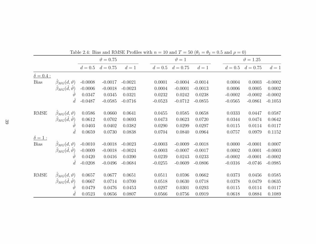
number of cross-section units and T is the length of time series. We explore the small-sample

behaviour of our estimates by means of Monte Carlo experiments both when autocorrelations

and/or endogeneity are absent and present, and find that the estimates behave well even in

relatively small panels.

In the empirical application, we investigate the long-run relationship between real GDP and

debt/GDP growth rates as well as debt and real GDP in log-levels for 20 high-income OECD

countries for the time period 1955-2008. We find that GDP growth does not respond to a growth

in debt/GDP for most of the countries at the 5% level. On the other hand, real GDP and debt in

log-levels have a significant relationship for all countries but New Zealand and the United States,

and this relationship is cointegrating for several countries, which we can find using our panel

approach but not using a pure time series cointegration methodology as we show comparing our

results to those that would be obtained by Hualde and Robinson [22]’s method. The empirical

application stresses that our panel data approach provides correct inference particularly when the

main source of persistence in the indicators is cross-country dependence.

The remainder of the paper proceeds as follows. Next section contains estimation details of

slope and fractional integration parameters. Section 2.3 lists all the conditions needed and contains

the main results. Section 2.4 briefly discusses the inclusion of deterministic trends. Section 2.5

presents a finite-sample study based on Monte Carlo experiments, and Section 2.6 presents the

empirical application. Section 2.7 contains the final comments.

Throughout the paper, “(n, T )j” denotes joint asymptotics in which both the cross-section

size and time-series length are growing; “ →p ” denotes convergence in probability; and “ →d ”

denotes convergence in distribution. All mathematical proofs and intermediate technical results

are collected in an appendix at the end of the paper.

2.2 Model, Discussion and Parameter Estimation

We consider the following triangular array describing a type-II fractionally integrated panel data

model of the observed series (yit, xit) :

yit = αi + xitβi0 + ftλi + ∆−di0t ε1it, (2.1)

xit = µi + ftγi + ∆−ϑi0t ε2it,

3

where yit and xit are scalars whose idiosyncratic innovations have unknown true integration orders

di0 and ϑi0 for i = 1, . . . , n and t = 1, . . . , T, and ft is an unobserved common factor that may be

integrated of an unknown order δ. While vector xit may also be analyzed allowing for a multiple

regression setting, we consider the simplest case to focus on the main ideas. Throughout the

paper, the subscript at the fractional differencing operator attached to a vector or scalar εit (i.e.

a type-II process) has the meaning

∆−dt εit = ∆−dεit1(t > 0) =t−1∑j=0

πj(−d)εit−j, (2.2)

πj(−d) =Γ(j + d)

Γ(j + 1)Γ(d),

where 1(·) is the indicator function, and Γ(·) denotes the gamma function such that Γ(d) = ∞for d = 0,−1,−2, . . . , and Γ(0)/Γ(0) = 1 by convention. With the prime denoting transposition,

εit = (ε1it, ε2it)′ is a bivariate covariance stationary process, allowing for Cov(ε1it, ε2it) 6= 0, whose

short-memory vector-autoregressive (VAR) dynamics are described by

B(L; θi)εit ≡

(I2 −

p∑j=1

Bj(θi)Lj

)εit = vit, (2.3)

where L is the lag operator, θi the short-memory parameters, I2 the 2× 2 identity matrix, Bj the

2×2 upper-triangular matrices, and vit is a bivariate sequence that is identically and independently

distributed across i and t with zero mean and covariance matrix Ωi > 0. The upper-triangularity

assumption on the short-memory matrices, Bj, provides a great deal of parsimony in the asymp-

totics as it further develops the triangular structure of the system, and it is in line with the

long-run VAR restriction of Blanchard and Quah [7] and the short-run VAR restriction of Sims

[40]. The arrays αi, i ≥ 1 and µi, i ≥ 1 are unobserved individual fixed effects; ft, t > 0is the I(δ) unobserved common factor that induces cross-section dependence and possibly further

endogeneity in the system; λi, i ≥ 1 and γi, i ≥ 1 are unobserved factor loadings indicating

how much each cross-section unit is affected by ft. In addition to these general dynamics, au-

toregressive conditional heteroskedasticity can also be featured in the common factor so that the

model can be suitable also for applications in finance.

After explaining the technical details of the model, it is also important to show the usefulness of

it in economic analysis. First, the panel data model in (2.1) nests stationary I(0) and nonstationary

I(1) autoregressive panel data models that are extensively used in economic modelling, but unlike

in the I(1) autoregressive case, (2.1) has smoothness everywhere, thus the test statistics for the

parameter estimates obtained under (2.1) are χ2 distributed. Second, allowance for general long-

range dependence through model innovations and the common factor structure is mainly motivated

by a desire to avoid a priori unit-root or stationarity testing as is currently carried out in empirical

analyses dealing with possibly nonstationary variables. Third, parameter heterogeneity in (2.1)

4

allows for obtaining unit-specific inference in an economy while latent individual characteristics

and possible interactions of the units are also taken into account through fixed effects and common

factor structures. Heterogeneity in the memory parameters allows for each unit to exhibit different

persistence characteristics. This contrasts with the standard approach in the literature when a

nonstationary variable is assumed to be I(1) for all cross-section units merely based on unit-root

testing.

2.2.1 Prewhitening and Projection of the Common Factor Structure

In a standard way, we first-difference (2.1) to remove the fixed effects,

∆yit = ∆xitβi0 + ∆ftλi + ∆1−di0t ε1it, (2.4)

∆xit = ∆ftγi + ∆1−ϑi0t ε2it,

for i = 1, . . . , n and t = 2, . . . , T. After this transformation, it becomes clear that there is a

mismatch between the sample available and the lengths of the fractional filters ∆1−di0t and ∆1−ϑi0

t ,

which involve ε1i1 and ε2i1, i.e. the initial conditions, while in practice only the filter ∆t−1 can

be used. We argue that initial conditions in the idiosyncratic innovations are negligible since the

second-order bias caused by initial conditions asymptotically vanishes in time-series length under

a heterogeneous setup; see Ergemen and Velasco [16].

Setting

ϑmax = maxiϑi and dmax = max

idi,

(2.4) can be prewhitened from idiosyncratic long-range dependence for some fixed exogenous

differencing choice, d∗, using which all variables become asymptotically stationary with their

sample means converging to population limits.

Let us introduce the notation ait(τ) = ∆τ−1t−1 ∆ait for any τ. Then the prewhitened model is

given by

yit(d∗) = xit(d

∗)βi0 + ft(d∗)λi + ε1it(d

∗ − di0), (2.5)

xit(d∗) = ft(d

∗)γi + ε2it(d∗ − ϑi0).

Thus, using the notation zit(τ1, τ2) = (yit(τ1), xit(τ2))′ , (2.5) can be written in the vectorized

form as

zit(d∗, d∗) = ζxit(d

∗)βi0 + Ft(d∗)Li + εit (d∗ − di0, d∗ − ϑi0) , (2.6)

where ζ = (1, 0)′, Ft(d∗) = ft(d

∗)⊗ I2, Li = (λi, γi)′, and ft, λi and γi are scalars.

The structure Ft(d∗)Li in (2.6) induces cross-section correlation between units i through Ft(d

∗).

5

The common factor may also be allowed to feature breaks both at levels and in persistence under

higher order assumptions, which we do not explore in this paper. Several techniques for eliminating

or estimating I(0) common-factor structures have been proposed in the literature. Pesaran [29]

suggests using cross-section averages of the observed series as proxies to asymptotically replace

the common factor structure. A different version of this procedure has been recently adopted in

case of persistent common factors by Ergemen and Velasco [16]. There has also been some focus

on estimating the factor loadings and common factors up to a rotation, in I(0) or I(1) cases,

which enables their use as plug-in estimates. The well-known principal components approach

(PCA) has been greatly extended in factor analysis by e.g. Bai and Ng [4] and Bai and Ng

[6]. While factor structure estimates, obtained by principal components analysis, can be used as

plug-in estimates thus allowing for the exploitation of more information in forecasting studies,

they cause size distortions leading to lower finite-sample performance in testing as pointed out by

Pesaran [29]. Moreover, PCA estimation of factors with fractional long-range dependence has not

been explored in the literature yet. Bearing in mind this fact, we project out the common factor

structure using the cross-section averages of prewhitened data, by which the projection errors

vanish asymptotically in cross-section size.

The estimation methodology is primarily based on proxying the latent common factor structure

using projections. To give the details about projection, let us denote zt(d∗, d∗) = n−1

∑ni=1 zit(d

∗, d∗)

to write (2.6) in cross-section averages as

zt(d∗, d∗) = ζxt(d∗)β0 + Ft(d

∗)L+ εt (d∗ − d0, d∗ − ϑ0) , (2.7)

where εt (d∗ − d0, d∗ − ϑ0) is Op(n

−1/2) for large enough d∗. Thus, zt(d∗, d∗) and ζxt(d∗)β0 asymp-

totically capture all the information provided by the common factor provided that L is full rank.

Note that xt(d∗) is readily contained in zt(d

∗, d∗) and βi0 do not have any contribution in terms

of dynamics in ζxt(d∗)β0 since they are fixed for each i. This is why, zt(d∗, d∗) alone can span the

factor space.

Let us write the time-stacked observed series as xi(d∗) = (xi2(d∗), . . . , xiT (d∗))′ and zi(d

∗, d∗) =

(zi2(d∗, d∗), . . . , ziT (d∗, d∗))′ for i = 1, . . . , n. Then, for each i = 1, . . . , n,

zi(d∗, d∗) = xi(d

∗)βi0ζ′ + F(d∗)Li + Ei (d

∗ − di0, d∗ − ϑi0) , (2.8)

where Ei (d∗ − di0, d∗ − ϑi0) = (εi2 (d∗ − di0, d∗ − ϑi0, ) , . . . , εiT (d∗ − di0, d∗ − ϑi0))′ and

F(d∗) = (vec [F2(d∗)] , . . . ,vec [FT (d∗)])′ .

The common factor structure, for T1 = T − 1, can asymptotically be removed by the T1 × T1

projection matrix

MT1(d∗) = IT1 − z(d∗, d∗)(z′(d∗, d∗)z(d∗, d∗))−z′(d∗, d∗), (2.9)

where z(d∗, d∗) = n−1∑n

i=1 zi(d∗, d∗), and P− denotes the generalized inverse of a matrix P. When

6

the projection matrix is built with the original (possibly nonstationary) series, it is impossible

to ensure the asymptotic replacement of the latent factor structure by cross-section averages

because the noise in (2.6) may be too persistent when d∗ = 0. On the other hand, using some

d∗ > maxϑmax, dmax, δ − 1/4 for prewhitening guarantees that the projection errors vanish

asymptotically.

Based on (2.8), the defactored observed bivariate series for each i = 1, . . . , n,

zi(d∗, d∗) = xi(d

∗)βi0ζ′ + Ei (d

∗ − di0, d∗ − ϑi0) , (2.10)

where zi(d∗, d∗) = MT1(d

∗)zi(d∗, d∗), xi(d

∗) = MT1(d∗)xi(d

∗) and Ei(d∗) = MT1(d

∗)Ei(d∗). The

projection error, MT1(d∗)F(d∗), is of order Op

(n−1 + (nT )−1/2

)as shown in Appendix A.1.

2.2.2 Estimation of Linear Model Parameters

Writing (2.10) for i = 1, . . . , n, and t = 2, . . . , T we now integrate the defactored series back by d∗

to their original integration orders, to perform estimations, as

z∗it(di, ϑi) = ζx∗it(di)βi0 + ε∗it (di − di0, ϑi − ϑi0) , (2.11)

where the first and second equations of (2.11) are obtained, respectively, by

y∗it(di) = ∆di−d∗t−1 yit(d

∗) and x∗it(ϑi) = ∆ϑi−d∗t−1 xit(d

∗),

where we omit the dependence on d∗ in the notation and assume away the initial conditions.

To explicitly show the short-memory dynamics in the model based on (2.3), (2.11) can be

written as

z∗it(di, ϑi)−p∑j=1

Bj(θi)z∗it−j(di, ϑi) (2.12)

=

ζx∗it(di)−

p∑j=1

Bj(θi)ζx∗it−j(di)

βi0 + v∗it (di − di0, ϑi − ϑi0) ,

whose second equation, noting that z∗it(di, ϑi) = (y∗it(di), x∗it(ϑi))

′, is

x∗it(ϑi)−p∑j=1

B2j(θi)z∗it−j(di, ϑi) =

(−

p∑j=1

B2j(θi)ζx∗it−j(di)

)βi0 + v∗2it (ϑi − ϑi0) (2.13)

and the first equation can be organized to account for the contemporaneous correlation if we write

7

y∗it(di)− ρix∗it(ϑi) as

y∗it(di) =x∗it(di)βi0 + x∗it(ϑi)ρi +

p∑j=1

(B1j(θi)− ρiB2j(θi)) z∗it−j(di, ϑi) (2.14)

−

(p∑j=1

(B1j(θi)− ρiB2j(θi)) ζx∗it−j(di)

)βi0 + v∗1it (di − di0)− ρiv∗2it (ϑi − ϑi0)

with Bkj denoting the k-th row of Bj, and ρi = E[v∗1itv∗2it]/E[v∗2it

2].

Under (2.14), cointegration (i.e. ϑi0 > di0) is useful in the estimation of βi0 since the signal

that can be extracted from x∗it(di) is stronger than that from x∗it(ϑi). However, identification of βi0

is still possible in a spurious regression where di0 > ϑi0 since the error term in (2.14) is orthogonal

to v∗2it(·) given that vit are identically and independently distributed so that v∗1it (·) − ρiv∗2it (·)

is uncorrelated with v∗2it(·). The only exclusion we have under a spurious setting is the case in

which ϑi0 = di0, which leads to collinearity in (2.14) thus rendering the identification of βi0 and

ρi impossible. The spurious estimation case in which di0 > ϑi0 is evidently more relevant when

the interest is in the estimation of contemporaneous correlations between series more than in the

estimation of slope parameters. While the triangular array structure of the system readily leads to

the identification of βi0 and ρi so long as ϑi0 6= di0, some Bkj may still be left unidentified. In that

case, imposing an upper-triangular structure in Bj(·) to further develop the triangular structure

of the system leads to identification of Bkj.

The case in which ρi = 0, corresponding to exogenous regressors, has been developed by Erge-

men and Velasco [16], where estimation is carried out for the parameters only in the first equation

and ϑi are treated as nuisance parameters. In the present paper, while the main parameter of

interest is still βi0, we can also obtain the estimates of di0, ϑi0, ρi and Bj(θi).

In this paper, short-memory dynamics are not our main concern so we treat Bj(·) as nuisance

parameters. First, we use a q× (3p+ 2) restriction matrix Q that is I3p+2 when there are no prior

zero restrictions on Bj, and a q < 3p + 2 matrix with prior zero restrictions that is obtained by

dropping rows of Q corresponding to restrictions, which may improve efficiency by eliminating

some lagged values of the series. Then, write (2.14) as

y∗it(di) = ω′iQZ∗it(di, ϑi) + v∗1it (di − di0)− ρiv∗2it (ϑi − ϑi0) (2.15)

with

Z∗it(di, ϑi) =(x∗it(di), x

∗it(ϑi), u

∗′it−1(di, ϑi), . . . , u

∗′it−p(di, ϑi)

)′,

u∗it−k(di, ϑi) =(x∗it−k(di), x

∗it−k(ϑi), y

∗it−k(di)

)′, k = 1, . . . , p,

and ωi being the vector of coefficients that are functions of βi, ρi and Bkj(θi) whose least-squares

8

estimate is given by

ωi(τ1, τ2) := Mi(τ1, τ2)−1mi(τ1, τ2) (2.16)

with

Mi(τ1, τ2) = Q1

T

T∑t=p+1

Z∗it(τ1, τ2)Z∗′it (τ1, τ2)Q′ and mi(τ1, τ2) = Q1

T

T∑t=p+1

Z∗it(τ1, τ2)y∗it(τ1)

where (τ1, τ2) denotes the infeasible cases of (di0, ϑi0), (di, ϑi0), (di0, ϑi) and the feasible case of

(di, ϑi).

In most empirical work, the main parameter of interest is βi0, for which the estimate can simply

be obtained from (2.16) as

βi(τ1, τ2) = ψ′βωi(τ1, τ2), ψβ = (1, 0, . . . , 0)′ . (2.17)

While βi in (2.17) is less efficient than the Gaussian maximum likelihood estimate in the VAR εit

case, it is computationally much simpler in practice. Ergemen and Velasco [16] discuss the case

in which βi is efficient when Cov(ε1it, ε2it) = 0.

When the interest is in the estimation of contemporaneous correlation between the idiosyncratic

innovations, the vector ψ can be adjusted accordingly so that

ρi(τ1, τ2) = ψ′ρωi(τ1, τ2), ψρ = (0, 1, . . . , 0)′ .

Short-memory matrices Bj(θi) and, in case of knowledge on the mappings Bj(·), thereof short-

memory parameters can be estimated similarly taking e.g. ψθ = (0, 0, 1, . . . , 1)′ .

2.2.3 Estimation of Long-Range Dependence Parameters

For the estimation of long memory or fractional integration parameters, we only consider the

empirically relevant case of unknown di and ϑi. Estimation of long-range dependence parameters

in the panel data context is a relatively new topic. Robinson and Velasco [39] propose several

techniques for estimating a pooled fractional integration parameter under a fractional panel setting

with no covariates or cross-section dependence. Extending their study, Ergemen and Velasco [16]

propose fractional panel data models with fixed effects and cross-section dependence in which the

long-range dependence parameter is estimated, also when their general model features exogenous

covariates, in first differences.

In order to estimate both long-range dependence parameters under our setup, we use an

equation-by-equation CSS approach. First, we estimate the second equation of (2.12). Assuming

9

an upper-triangular structure for Bj(θi) in (2.3) for parsimony, we write (2.13) as

x∗it(ϑi)− φ′iRX∗it(ϑi) = v∗2it(ϑi − ϑi0)

with

X∗it(ϑi) =(x∗it−1(ϑi), . . . , x

∗it−p(ϑi)

)′,

the r × p matrix R = Ip for r = p, but for r < p, R is obtained by dropping rows from Ip, and φi

collecting the B22j that are nonzero a priori. Then an estimate of φi,

φi(ϑ) := Gi(ϑ)−1gi(ϑ) (2.18)

where

Gi(·) = R1

T

T∑t=p+1

X∗it(·)X∗′it (·)R′ and gi(·) = R1

T

T∑t=p+1

X∗it(·)x∗it(·).

Having obtained (2.18), ϑi0 can be estimated by

ϑi = arg minϑ∈V

T∑t=p+1

x∗it(ϑ)− φi(ϑ)′RX∗it(ϑ)

2

,

with V = [ϑ, ϑ] ⊂(0, 3

2

).

Then di0 can be estimated from (2.15) by

di = arg mind∈D

T∑t=p+1

y∗it(d)− ωi(d, ϑi)′QZ∗it(d, ϑi)

2

,

with D = [d, d] ⊂(0, 3

2

).

The lower-bound restrictions on the sets V and D, i.e. d, ϑ > 0, ensure that the initial-condition

terms are asymptotically negligible because they are of size Op(T−di) and Op(T

−ϑi). The upper-

bound restrictions are a consequence of the first-differencing transformation, which is mirrored by

working with d∗ ≥ 1.

The estimates ϑi and di are not efficient since they are not jointly estimated. To update the

estimates to efficiency, a single Newton step may be taken from these initial estimates, τi = (di, ϑi),

whose√T−consistency we establish in Section 3, as

τi = τi −H−1T (τi)hT (τi), (2.19)

10

where

HT (τ) =1

T

T∑t=1

(∂ ˆv∗it(τ)

∂τ ′

)′(1

T

T∑t=1

ˆv∗it(τ)ˆv∗it(τ)′

)−1

∂ ˆv∗it(τ)

∂τ ′,

and

hT (τ) =1

T

T∑t=1

(∂ ˆv∗it(τ)

∂τ ′

)′(1

T

T∑t=1

ˆv∗it(τ)ˆv∗it(τ)′

)−1

ˆv∗it(τ)

with

ˆv∗it(di, ϑi) = z∗it(di, ϑi)−p∑j=1

Bj(θi)z∗it−j(di, ϑi)−

ζx∗it(di)−

p∑j=1

Bj(θi)ζx∗it−j(di)

βi(di, ϑi).

2.2.4 Common Correlated Mean-Group Slope Estimate

In many empirical applications, there is also an interest in obtaining inference on the panel rather

than individual series alone. Given the linearity of the model in βi, we consider the common-

correlation mean-group estimate,

βCCMG

(d, ϑ)

:=1

n

n∑i=1

βi

(di, ϑi

). (2.20)

This estimate is essentially a GLS mean-group estimate based on the average of individual feasible

slope estimates. For the asymptotic analysis of the mean-group estimate, it is standard to use a

random coefficients model as in

βi = β0 + wi, wi ∼ iid (0,Ωw) ,

with wi independent of all other model variables.

2.3 Assumptions and Main Results

We impose and discuss a set of regularity conditions that allow us to derive our asymptotic results.

Assumption 1 (Long-range dependence and common-factor structure). Persistence and

cross-section dependence are introduced according to the following:

1. The fractional integration parameters, with true values ϑi0 6= di0, satisfy maxϑmax, dmax, δ−minϑ, d < 1/2, and either maxϑmax, dmax, δ < 5/4 with d∗ = 1, or d∗ > maxϑmax, dmax, δ−1/4.

11

2. The common factor vector satisfies ft = αf+∆−δt zft , where zft =∑∞

k=0 Ψfkεft−k with

∑∞k=0 k

∣∣∣Ψfk

∣∣∣ <∞, and εft ∼ iid(0, σf ), E

∣∣∣εft ∣∣∣4 <∞.3. ft and ε·it are independent, and independent of factor loadings λi and γi for all i and t.

4. Factor loadings λi and γi are independent across i, and the matrix(γβ + λ

γ

)

is full rank.

Assumption 1.1 is a fairly general version of the assumptions used by e.g. Hualde and Robinson

[23] and Nielsen [28], additionally ensuring that the projection errors asymptotically vanish with

the prescribed choice of d∗. To simplify the presentation, we consider a large enough d∗ prescribed

in Assumption 1.1 without pointing out a fixed value although for most applications d∗ = 1 would

suffice anticipating ϑi0, δ, di0 < 5/4. This condition also requires that the lower bounds of the sets

V and D not be too apart from other memory parameters when di0 ∈ D and ϑi0 ∈ V , in which

case it is further implied that ϑi0 − di0 < 1/2, i.e. at most weak fractional cointegration.

Assumption 1.2 allows for long-range dependence in the common factors that may also have

short-memory dynamics, where the I(0) innovations of ft are not collinear. The restriction on the

number of factors may be relaxed when more covariates are introduced: in general, if there are r

covariates, the maximum number of factors that can be featured is 1 + r so that the factor space

can be spanned. The non-zero mean possibility in the common factor, i.e. when αf 6= 0, allows

for a drift in the common factor.

Assumptions 1.3 and 1.4 are standard in the factor models literature and have been used by

e.g. Pesaran [29] and Bai [2]. The full rank condition on the factor loadings matrix simplifies

the identification of factors with no loss of generality requiring that there be sufficiently many

covariates whose sample averages can span the factor space. This is straightforwardly satisfied in

case of one common factor.

Assumption 2 (System errors). The process εit has the representation

εit = Ψ(L; θi)vit

where

Ψ(s; θi) = I2 +∞∑j=1

Ψj(θi)sj

and the 2× 2 matrices Ψj satisfy that

1.∑∞

j=1 j ‖Ψj‖ <∞, det Ψ(s; θi) 6= 0, |s| = 1 for θi ∈ Θ;

12

2. Ψ(L; θi) is twice continuously differentiable in θi on a closed neighborhood Nr(θi0) of radius

0 < r < 1/2 about θi0;

3. the vit are identically and independently distributed vectors across i and t with zero mean

and positive-definite covariance matrix Ωi, and have bounded fourth-order moments.

Assumptions 2.1-2.3 are quite standard in the analysis of stationary VAR processes, as were

also used by Robinson and Hualde [38], constituting the counterpart conditions for Bj. The first

condition rules out possible collinearity in the innovations imposing a standard summability re-

quirement and ensures well-defined functional behaviour at zero frequency, allowing for invertibil-

ity. The second condition is needed for the uniform convergence of the Hessian in the asymptotic

distribution, and finally the moment requirement in the third condition is in general easily satis-

fied under Gaussianity. The iid requirement in the last condition may be relaxed to martingale

difference innovations whose conditional and unconditional third and fourth order moments are

equal, which indicates iid behaviour up to fourth moments.

Assumption 3 (Rank condition). Based on the time-stacked version of the vector of observables

Z∗it, Z∗i , the following conditions are satisfied:

1. T−1Z∗i Z∗′i is full rank;

2.(T−1Z

∗i Z∗′i

)−1

has finite second order moments.

Assumption 3.1 is a regularity condition ensuring the existence of the least-square estimate

in (2.16) and thus of the slope estimate in (2.17) while Assumption 3.2 is used in the derivation

of asymptotic results of the common-correlation mean group estimate described in (2.20). These

conditions are used by Pesaran [29] based on stationary I(0) variables.

Under our setup, the common-factor structure that accounts for cross-sectional dependence is

projected out, and this adds the extra complexity of dealing with projection errors. In a pure

time-series context, Hualde and Robinson [22] derive joint asymptotics for memory and slope

parameters without accounting for individual or interactive characteristics of the series. Although

the results by Hualde and Robinson [22] are similar to ours, showing our results relies heavily on

the projection algebra due to the allowance of cross-section dependence.

The next theorem presents the consistency of slope and long-range dependence parameter

estimates that are mainly of interest in structural estimation.

Theorem 1. Under Assumptions 1-3, as (n, T )j →∞,βi(di, ϑi)− βi0

di − di0ϑi − ϑi0

→p 0.

13

This result does not require a rate condition on n and T so long as they jointly grow in the

asymptotics, and it can be readily extended to include also the other model parameters. This

contrasts with the results derived by Robinson and Velasco [39], where only T is required to

grow and n can be fixed or increasing in the asymptotics. An increasing T is needed therein

since it yields the asymptotics, as is needed here, but projection on cross-section averages for

factor structure removal further requires that n grow because the projection errors are of size

Op

(n−1 + (nT )−1/2

)as shown in Appendix A.1.

Next, we show the joint asymptotic distribution of the parameters, where a rate condition on

n and T is imposed to remove the projection error.

Theorem 2. Under Assumptions 1-3, and if√T/n→ 0 as (n, T )j →∞,

√T

βi(di, ϑi)− βi0

di − di0ϑi − ϑi0

→d N (0, AiBiA′i) .

The variance-covariance matrix AiBiA′i has a highly involved analytic expression, but defini-

tions of the estimates Ai and Bi, thus forming the positive semi-definite covariance matrix estimate

AiBiA′i, are provided in Appendix 2.8.4.

This joint estimation result differs from the one by Robinson and Hualde [38] but is similar

to that by Hualde and Robinson [22] in that there can at most be weak cointegration under

our setup. Removal of common factors that allow for cross-section dependence brings the extra

condition that Tn−2 → 0 along with more involved derivations, leading to substantially different

proofs from those only outlined in Hualde and Robinson [22]. Under lack of autocorrelation and

endogeneity induced by the idiosyncratic innovations, Ergemen and Velasco [16] establish the√T -

convergence rate in the joint estimation of both slope and fractional integration parameters under

weak cointegration, with which our results are also parallel.

We finally consider the asymptotic behaviour of the common correlated mean-group slope

estimate.

Theorem 3. Under Assumptions 1-3, as (n, T )j →∞,

√n(βCCMG

(d, ϑ)− β0

)→d N (0,Ωw) .

This theorem extends the results by Pesaran [29] and Kapetanios et al. [24] on I(0) and I(1)

variables, where this GLS-type estimate now converges at the√n rate without requiring any

14

conditions on the relative growth of n to T. The asymptotic variance-covariance matrix, Ωw, can

be estimated nonparametrically based on the GLS slope estimates by

Ωw

(d, ϑ

)=

1

n− 1

n∑i=1

(βi

(di, ϑi

)− βCCMG

(d, ϑ

))(βi

(di, ϑi

)− βCCMG

(d, ϑ

))′since variability only depends on the heterogeneity of the βi, and bold indicates parameter vectors.

2.4 Deterministic Trends

While our model in (2.1) can accommodate both deterministic and stochastic unobserved trends

via the common factor ft, this imposes that the trending behaviour be shared by some cross-

section units, in particular by those with nonzero factor loadings. This then indicates that among

those cross-section units sharing the same trend, the difference is only up to a constant, based on

λi and γi. To relax such a restriction and allow for separate time trends, we extend the model in

(2.1) as

yit = αi + α1i q(t) + xitβi0 + ftλi + ∆−di0t ε1it, (2.21)

xit = µi + µ1i r(t) + ftγi + ∆−ϑi0t ε2it,

where now q(t) and r(t) are known time trends.

The case in which q(t) and r(t) in (2.21) are linear, possibly with drifts, can be straightforwardly

analyzed in second differences, at whose first and second differences the time trends are reduced

to constants and removed, respectively. Alternatively, projections can be carried out in first

differences using an augmented version of the projection matrix described in (2.9) to include ones

at its first column, which then mirrors fixed-effects estimation in first differences. In both of these

approaches, asymptotics remain the same under the conditions prescribed in Section 2.3: although

the series may be overdifferenced in the beginning, they are integrated back by the order of their

initial differencing orders after projections to their original integration orders, e.g. for double

differencing, as in

∆d−2t−1 ∆2yit ≈ ∆d

t−1yit and ∆ϑ−2t−1 ∆2xit ≈ ∆ϑ

t−1xit.

In cases of (possibly fractional) nonlinearity in q(t) and r(t), such as t2, t3, log t and ∆−ϕ1

with ϕ > 1/2, removal or estimation of trends may become more complicated as opposed to the

linear case. When the orders of trend polynomials are known, the first column of the projection

matrix in (2.9) can be augmented accordingly to remove the trending behaviour. Even when q(t)

and r(t) are functional trends of known orders, such projection matrix augmentation may prove

useful. However, when the orders of trend polynomials are unknown, removal of trends based on

projection is not straightforward, though some nonparametric GLS detrending approach might be

15

used. This case is beyond the scope of the present paper and is not further explored.

2.5 Simulations

In this section, we investigate the finite-sample behaviour of our estimates, βi(di0, ϑi0), di, ϑi and

βi(di, ϑi), by means of Monte Carlo experiments. While we estimate the parameters for each

i separately, we can only report the average characteristics. We draw the mean zero Gaussian

idiosyncratic innovations vector vit with covariance matrix

Ω =

(a11 a12

a21 a22

),

where we allow for variations in the signal-to-noise ratio, τ = a22/a11, and the correlation ρ =

a12/(a11a22)1/2. We take a11 = 1 with no loss of generality, and introduce the short-memory

dynamics taking Bj(θi) = diag θ1i, θ2i to generate εit.

We draw the factor loadings as U(−0.5, 1), and then generate serially correlated common

factors based on iid innovations drawn as standard normal. The fixed effects are left unspecified

since projections and estimations are carried out in first differences. Fixing the cross-section size

and time-series length to n = 10 and T = 50, respectively, we consider the parameter values

ϑ = 0.75, 1, 1.25, d = 0.5, 0.75, 1, covering both cointegration and noncointegration cases, and

θ1 = θ2 = 0, 0.5 with ρ = 0, 0.5 for δ = 0.4, 1. For this study, we fix βi0, τ, d∗ = 1. Simulations are

carried out via 1,000 replications.

Tables 2.1 and 2.2 present the bias and RMSE profiles of our estimates for θ1 = θ2 = ρ = 0 and

θ1 = θ2 = ρ = 0.5, respectively. Both the feasible and infeasible versions of βMG have considerably

small biases under absence of autocorrelation and endogeneity, with the biases further decreasing

in ϑ although their magnitudes increase in δ. In the second setup, where both endogeneity and

autocorrelation are present, biases of all parameter estimates show an increase in magnitude due

to the simultaneous equation bias stemming from prevalent contemporaneous correlations. Biases

of slope estimates are decreasing in the order of cointegration, i.e. ϑ−d. The fractional parameter

estimate ϑ remains robust in terms of bias for a given ϑ, and the estimate d has a bias generally

decreasing in d.

In terms of performance, slope estimates behave well both under absence and presence of

autocorrelation and endogeneity, in most cases standard deviations dominating biases in terms of

contribution to root mean square errors (RMSE). The fractional parameter estimates ϑ and d also

perform well.

In order to investigate the contributions of endogeneity and short-memory dynamics separately,

we next consider θ1 = θ2 = 0 with ρ = 0.5 as well as θ1 = θ2 = 0.5 with ρ = 0. Table 2.3 presents the

case of endogeneity without short-memory dynamics. Compared to the results in Table 2.1, slope

estimates mainly suffer from the simultaneous equation bias caused by ρ 6= 0 while the performance

of fractional integration parameters are slightly ameliorated. When autocorrelation is introduced

16

instead of endogeneity in Table 2.4, slope estimates perform similarly to the results in Table

2.1. The performance of fractional parameter estimates ϑ and d, however, are slightly worsened

compared to the results in Table 2.1. A further comparison between Tables 2.2 and 2.3 reveals that

under endogeneity, short-memory dynamics help both the feasible and infeasible slope estimates

in terms of performance in some cases. Introducing endogeneity when short-memory dynamics are

already present improves the performance of fractional integration parameter estimates to some

extent as can be concluded from the comparison of Tables 2.2 and 2.4.

We also explore the finite-sample behaviour of our estimates under (2.21) taking r(t), q(t) = t.

As before, estimations are performed in first differences, but the projection matrix in (2.9) is now

augmented to include ones in its first column. This way, the estimation method mimics fixed-

effects estimation in first differences, and the corresponding bias and RMSE profiles are shown

in Tables 2.5 and 2.6. The results in Tables 2.5 and 2.1 are comparable as are the results in

Tables 2.6 and 2.2. With the inclusion of linear trends, while both the infeasible and feasible slope

estimates have positive and small biases, the fractional integration parameter estimates appear to

have been underestimated in general.

Finally, we replicate the results in Table 2.2 taking n = 5 and T = 25 to explore the small-

sample behaviour of the estimates in the most difficult case since the projection errors have a

larger role. These results are reported in Table 2.7. In terms of performance, the standard errors

roughly double (although for individual estimates the convergence rate is√T , through averaging

the rate becomes approximately√nT ) while the bias profiles of slope estimates remain more or

less the same. However, fractional integration parameter estimates generally suffer from larger

biases compared to the results in Table 2.2.

2.6 An Analysis of the Long-Run Debt and GDP Rela-

tionship

2.6.1 Related Literature and Empirical Strategy

The relationship between debt and economic growth has been extensively analyzed based on

several different approaches leading to mixed results. Among many others, Elmendorf and Mankiw

[14] argue for the negative effect of public debt on growth. Reinhart and Rogoff [33] use a

debt-bracketing approach coupled with threshold estimation to conclude that high debt hinders

economic growth in developed countries. Baglan and Yoldas [1] show that nonlinearities caused by

a common debt-level threshold is insignificant and suggest grouping the countries according to their

debt-to-GDP ratios to conclude a common negative relationship between GDP growth and debt

for countries with chronically high debt. In line with these findings, Chudik et al. [11] show that

debt has a negative and significant effect on growth in the long-run and that debt-level thresholds

have no significant effects thus refuting the nonlinearity arguments based on thresholding in debt

dynamics. Contrary to these views, DeLong and Summers [13] find a positive effect of debt on

17

GDP growth arguing that recession periods can lead to a situation in which expansionary fiscal

policies may have positive effect on long-run GDP growth.

Overall the existing literature has provided ambiguous conclusions as to whether the rela-

tionship between debt and GDP growth is negative or positive due to large differences in their

estimation methodologies. Except for the econometric specification by Chudik et al. [11], which

constitutes the AR alternative of ours, all others rely on homogeneous slope estimation methods,

completely disregarding country characteristics and possible interactions between countries. Such

homogeneity assumption on the slope parameter implies that different countries converge to their

equilibrium at the same rate and that there is no debt overhang from one country to another,

which is implausible given the increasing interdependencies between economies. Although Chudik

et al. [11] can address these issues in their cross-sectionally augmented autoregressive distributed

lag estimation strategy, they restrict their analyses to I(0) and I(1) assumptions. Just like in

the other references, their decision on the stationarity of the dynamics of debt-to-GDP ratio and

GDP growth is merely based on unit-root testing. However, as is well known by now, rejecting

the null of a unit root does not imply I(0) stationarity in the series since stationarity may also

be rejected. Our methodology does not require a priori unit-root or stationarity testing because

these and in-between cases are flexibly nested.

We analyze the relationship between real GDP and debt-to-GDP growth rates and the rela-

tionship between real GDP and debt in log-levels separately in the following subsections. The

former application is aimed at contrasting our findings to those in the literature, and the latter

is included for the sake of simplicity in interpretations. In the first part, we use post-war yearly

data on debt-to-GDP ratios from Reinhart’s database and real GDP data from Angus Maddi-

son’s website spanning the time period 1955-2008 for 20 high-income OECD countries: Australia,

Austria, Belgium, Canada, Denmark, Finland, France, Germany, Greece, Ireland, Italy, Japan,

Netherlands, New Zealand, Norway, Portugal, Spain, Sweden, United Kingdom and United States.

Real GDP growth rates and debt-to-GDP ratios for each country are plotted in Figures 1 and 2,

respectively. In the second part using the same datasets, we use the PPP-based GDP data and

construct debt data based on that and debt/GDP data for the time period 1955-2008. Since using

only level data might invalidate the results if residuals obtained from regressions are trending, we

perform the analysis in logs to ensure this is not the case.

2.6.2 Empirical Analysis of the GDP Growth and Debt-to-GDP Ratio

Relationship

We examine the effect of debt1 on economic growth using our fractionally integrated panel data

estimation methodology. Using our approach, we incorporate country-specific characteristics and

the interactions between countries while also allowing for endogeneity without having to restrict

1We use data on central government debt since this is the only available data for all the high-income OECDcountries that we consider.

18

our analysis to I(0) and I(1) cases, by which we are able to detect stationarity and nonstationarity

of fractional orders.

From Figures 1 and 2, it is evident that real GDP growth rates show more oscillations, which

is a typical behaviour of stationary series, than debt-to-GDP ratios for all countries. The average

growth rate for all countries over time is 3.37% while the average debt-to-GDP ratio is 53.21%. In

line with the literature, the correlation coefficient between these averaged series is -0.0983 implying

an inverse relationship between debt and growth. Furthermore, we account for cross-section mean

and variance characteristics of the series so that we can get accurate inference on the long-run

relationship between growth rates and debt-to-GDP ratios, if any.

First, we estimate the fractional integration orders of real GDP growth rates and debt-to-

GDP ratios using local Whittle estimation based on Robinson [35] with bandwidth choices of

m = 10, 14. Given that the sample contains 54 time-series data points, choosing higher Fourier

frequencies will lead to short-memory contamination in the estimates. The estimation results are

collected in Table 8.

The results in Table 8 suggest that real GDP growth rates may in fact be integrated of fractional

orders and even be mildly nonstationary2 although they are always considered to be I(0) variables

in the literature. While the null of I(0) stationarity in GDP growth rates cannot be rejected

for several countries given the standard errors of their memory estimates, there are also other

countries in our sample whose growth rates are significantly fractionally integrated of different

orders, thus justifying our approach.

The integration order estimates of debt-to-GDP ratios presented in Table 8 are all significant

and around unity, indicating high persistence but of varying orders. Chudik et al. [11] use debt-

to-GDP growth rates in their analysis, for which we present the integration orders also in Table

8. These fractional integration or memory estimates suggest that debt-to-GDP growth can still

be persistent for some countries with varying magnitudes.

We also estimate the fractional integration order of the common factor based on the cross-

section average of both of the series together, which proxy the factor structure well as is evident

from (2.7), using local Whittle estimation based on Robinson [35]. The common factor is integrated

of orders 0.7577 and 0.7067 for m = 10, 14, respectively, providing evidence that the cross-section

dependence is persistent itself, which has not been considered in this literature so far.

Having obtained the integration order estimates for GDP growth and debt-to-GDP ratio as

well as debt-to-GDP ratio growth, we analyze the relationship between real GDP growth rates

and debt-to-GDP growth rates, as is the case in Chudik et al. [11], for two reasons: first, re-

gressing GDP growth, which is stationary for most countries, on debt-to-GDP ratio, which is

highly nonstationary, is completely uninformative whereas a regression based on the change in the

debt-to-GDP ratio, which has almost the same persistence characteristics as GDP growth, can

prove insightful; second, interpretation of the results is more useful since our primary focus is on

2Chudik et al. [11] also point out that growth rates may be mildly nonstationary and use this information toselect sufficiently many lags in their ARDL specification.

19

determining how economic growth responds to a change in the debt-to-GDP ratio.

We therefore estimate (2.1) taking yit as the real GDP growth and xit as the debt-to-GDP

ratio growth of country i, based on our methodology in which we account for country-specific

characteristics, such as institutions and geographical location, as well as characteristics that are

common for all countries – OECD membership, high income, etc. Our estimation methodology

also allows for the two-way endogeneity between the debt-to-GDP ratio and real GDP growth

since the idiosyncratic innovations are allowed to be correlated in the model, which is called for in

this analysis as has been discussed by Baglan and Yoldas [1] and Chudik et al. [11]. The estimation

results, taking d∗ = 1.25 and assuming a VAR(1) structure in the idiosyncratic innovations, are

reported in Table 9. For all countries but Italy, slope coefficient estimates are insignificant at

the 5% level, indicating that debt-to-GDP growth and GDP growth do not have a relationship.

For Italy, the slope estimate is positive and significant, but the long-range dependence parameter

estimates are both insignificant, implying that the relationship between debt-to-GDP growth and

GDP growth only has a short-term nature.

Moreover, there is no statistically significant evidence for a cointegrating relationship between

economic growth and debt growth for any of the countries, which can be simply checked by means

of a t−test constructed as t = (ϑi − di)/s.e.(ϑi − di) in the direction ϑi > di. This leads to the

conclusion that there is no long-lasting equilibrium relationship between GDP growth and debt

growth. Along with most of the claims in the literature, this could be due to the net direction

of the causality between these variables being undetermined in the longer run: while high debt

burden may have an adverse impact on economic growth, low GDP growth (by reducing tax

revenues and increasing public expenditures) could also lead to high debt-to-GDP ratios.

2.6.3 Empirical Analysis of the Relationship between GDP and Debt

in Log-Levels

In structural estimation, using comparable level data, such as GDP and debt, leads to easy-to-

interpret results. With this in mind, we repeat the analysis in the previous subsection using real

GDP and debt in log-levels, whose persistence characteristics we expect to be similar, so that we

can identify possible long-run relationships. This way, we can guarantee that the results have

clear interpretations.

We find that both real GDP and debt levels exhibit different cross-section mean and volatility

characteristics, which we take into account so that valid comparisons can be made. We plot real

GDP and debt at levels after normalizations in Figures 3 and 4, respectively.

For both series, there is a clear trending behaviour, leading us to think that they are both

nonstationary series. To verify this, we carry out local Whittle estimations on logs of the level

series using m = 10, 14 Fourier frequencies. The results are collected in Table 10.

The estimation results show that real GDP and debt in logs are integrated of an order around

unity, which is in line with the literature where they are treated as I(1) variables. The common

20

factor of real GDP and debt is estimated based on the cross-section averages of the stacked

series and is integrated of orders 1.0042 and 0.9272 for m = 10, 14, respectively, indicating that

removing the common factor is essential for disclosing possible cointegrating relationships. To

verify this statement, we provide benchmark estimation results based on the pure time-series

estimation approach by Hualde and Robinson [22] assuming a VAR(1) structure. Along this line, to

understand the long-run relationships, we are interested in identifying cointegrating relationships.

Nontrivial cointegrating relationships between real GDP and debt exist if a) the slope coefficients

are significantly different from zero; b) the estimated integration orders of debt in log-levels are

significantly larger than those of the estimation residuals, i.e. ϑi > di. These benchmark estimation

results are collected in Table 11.

According to the results in Table 11, all the estimates are significant for all countries except

Australia and Canada with mixed signs. From these results, it is further indicated that real GDP

and debt in logs do not have a cointegrating relationship for any of the countries, which can be

simply checked by means of a t−test constructed as t = (ϑi − di)/s.e.(ϑi − di) in the direction

ϑi > di. This result can be explained as follows. A time-series regression conceptually omits the

common-factor structure accounting for cross-section dependence and when the common factor is

the main source of persistence, the resulting regression residuals turn out to be persistent thus

hindering the identification of a possible cointegrating relationship.

Now, using our model, we check the long-run relationship between real GDP and debt in logs,

again assuming a VAR(1) structure. These estimation results are reported in Table 12.

A positive (or negative) slope estimate indicates that a unit-percent change in debt leads to an

increase (decrease) in real GDP by βi%. According to the estimation results in Table 12, we find

that debt and real GDP in logs have a significant relationship for all countries except New Zealand

and the United States. The significant effect of debt on GDP is positive for Belgium, Canada,

Finland, France, Germany, Ireland, Spain and Sweden, and it is negative and significant for the

remaining countries. While a negative and significant effect of debt on real GDP is generally

reported in the literature, a positive effect can be, for example, due to the debt increasing because

of government spending while also fuelling real GDP; also see DeLong and Summers [13].

The relationship between real GDP and debt does not have a cointegration nature for Australia,

Belgium, Canada, Finland, Netherlands, Norway and the United Kingdom, which suggests that

the significant interplay between the variables has a short-term nature. On the other hand, we find

a cointegrating relationship between real GDP and debt for Austria, Denmark, France, Germany,

Greece, Ireland, Italy, Japan, Portugal, Spain and Sweden. While it cannot exactly be claimed

that real GDP and debt have a long-term equilibrium relationship in the strict macroeconomic

terms when ϑi0 − di0 > 1/2, there still is a clear co-movement between these indicators.

To conclude, using our methodology we find that real GDP and debt have a cointegrating

relationship for several high-income OECD countries while the impact can be positive or negative

across countries. These cointegration findings contrast well to the benchmark estimation results

in Table 11 where we could not find any cointegration due to the negligence of individual country

21

characteristics and cross-country dependence. That is to say, if heterogeneity and interdepen-

dencies across countries are not taken into account in analyses of economic unions, as in a pure

time-series estimation, identifying the true nature of the relationships between these variables will

not be possible.

2.7 Final Comments

We have considered a fractionally integrated panel data system with individual stochastic com-

ponents and cross-section dependence, which allows for a cointegrated system analysis in the

defactored observed series. Although the present paper is quite general in that it incorporates long-

range dependence and short-memory dynamics with the allowance of deterministic time trends,

it nevertheless can be extended nontrivially in the following directions. The parametric factor

structure inducing cross-section dependence in our model may be assumed to have been approx-

imated by weak factors thus capturing spatial dependence in the idiosyncratic innovations; see

Chudik et al. [12]. While this is a theoretical possibility in (2.1) with additional conditions on

the common factor, ft, we do not analyze spatial dependence explicitly. Parametric modelling of

spatial dependence, see e.g. Pesaran and Tosetti [30], may provide further insights. Moreover, a

multiple regression framework can be considered through the allowance of vector xit whose ele-

ments display different degrees of persistence. While the extension is trivial when the entire vector

displays the same persistence characteristics, the treatment of unit-varying persistence is likely to

complicate the uniformity arguments shown in this paper. This extension, however, may allow

for the identification of multiple cointegrating relationships. Finally, the fractionally integrated

latent factor structure may be estimated and those estimates may be used as plug-in estimates in

drawing inference on other model parameters, thus allowing the model to be used in forecasting

studies. PCA estimation of fractionally integrated factor models are yet to be explored in the

literature.

2.8 Technical Appendix

2.8.1 Proof of Theorem 1

Projections are carried out based on (2.9). Denoting z(d∗, d∗) ≡ z(d∗), let us write

x′i(d∗)MT1(d

∗)F(d∗) = x′i(d∗)IT1F(d∗)− x′i(d

∗)z(d∗)(z′(d∗)z(d∗))−z′(d∗)F(d∗), (2.22)

with

z(d∗) = F(d∗)C + E (d∗ − d,d∗ − ϑ) (2.23)

22

where bold indicates the vector of parameters with the critical parameter values being dmax and

ϑmax, and

C =

γβ + λ 0

0 0

0 0

0 γ

and E (d∗ − d,d∗ − ϑ) = ε (d∗ − d,d∗ − ϑ) + ε2 (d∗ − ϑ) βζ ′.

Suppressing the notation as E (d∗ − d,d∗ − ϑ) ≡ E , the elements of the second term on the RHS

of (2.22) can be expressed as

T−11 x′i(d

∗)z(d∗) = T−11 x′i(d

∗)F(d∗)C + T−11 x′i(d

∗)E

T−11 z′(d∗)z(d∗) = T−1

1 C′F′(d∗)F(d∗)C + T−1

1 C′F′(d∗)E + T−1

1 E ′F(d∗)C + T−11 E ′E

T−11 z′(d∗)F(d∗) = T−1

1 C′F′(d∗)F(d∗) + T−1

1 E ′F(d∗).

By Assumption 2,

εt = Ψ(L;θ)vt, θ ∈ Θ,

with∑∞

j=1 j ‖Ψj‖ < K, where K is a positive constant. Thus, projections based on vt and εt incur

errors of the same asymptotic size, and we will show the results in this simpler case to motivate

the main ideas.

Then, by Lemma 1, as n→∞, the projection error, which is the sum of the terms containing

E , is of size

Op

(1

n+

1√nT

)= op(1).

Denote the projection matrix containing the true factors MF . By the idempotence of the projection

matrix, this result implies that

x′i(d∗)MT1(d

∗)F(d∗) = x′i(d∗)MFF(d∗) +Op

(1

n+

1√nT

), (2.24)

indicating that MT1 can replace MF as n → ∞, which is useful for the asymptotic analysis.

Furthermore,

T1/21 x′i(d

∗)MT1(d∗)F(d∗) = T

1/21 x′i(d

∗)MFF(d∗) +Op

(√T

n

). (2.25)

Using the projection arguments above, we first show the consistency of βi(di0, ϑi0), taking for

simplicity p = 0 together with the notation d = di0 and ϑ = ϑi0, corresponding to the unfeasible

23

LS estimate with no short-memory dynamics. Then in (2.14), denoting∑

t =∑T

t=2,

βi(d, ϑ) =

∑t x∗it

2(ϑ)∑

t x∗it(d)y∗it(d)−

∑t x∗it(d)x∗it(ϑ)

∑t x∗it(ϑ)y∗it(d)∑

t x∗it

2(d)∑

t x∗it

2(ϑ)− (∑

t x∗it(d)x∗it(ϑ))2 ,

from which we can write

βi(d, ϑ)− βi0 =

∑t x∗it

2(ϑ)∑

t x∗it(d)v∗1.2it −

∑t x∗it(d)x∗it(ϑ)

∑t x∗it(ϑ)v∗1.2it∑

t x∗it

2(d)∑

t x∗it

2(ϑ)− (∑

t x∗it(d)x∗it(ϑ))2 , (2.26)

where v∗1.2it = v∗1it−ρiv∗2it. Now noting that Cov (v∗2it, v∗1.2it) = 0, and using the projection arguments

above,

βi(d, ϑ)− βi0 = Op

(1√T

+1

n

)= op(1).

We then show the consistency of ϑi taking p = 0 because the proof follows exactly the same

steps for other p values. Write the time-stacked CSS as

Li,T (ϑ) =1

Tx∗i (ϑ)x∗′i (ϑ), (2.27)

for ϑ ∈ V = [ϑ, ϑ] ⊂(0, 3

2

). Now,

x∗i (ϑ) = ∆ϑ−d∗∆d∗−1∆xi,

where

∆d∗−1∆xi = ∆d∗−1∆xi − ςxz(d∗)

= ∆d∗−1∆xi −∆d∗−1∆xiz′(d∗)(z(d∗)z′(d∗))−1z(d∗)

so that

∆ϑ−d∗∆d∗−1∆xi = ∆ϑ−1∆xi − ςxz(ϑ).

Next, to be able to make use of (2.24), let us write

∆ϑ−1∆xi = Ix + Jx

with

Ix = ∆ϑ−ϑi0v2i −∆d∗−ϑi0v2iF′(d∗) (F(d∗)F′(d∗))

−1F(ϑ),

Jx = ∆d∗−ϑi0v2i

F′(d∗) (F(d∗)F′(d∗))

−1F(ϑ)− z′(d∗)(z(d∗)z′(d∗))−1z(ϑ)

24

where F(d∗) = (f2(d∗), . . . , fT (d∗))′ . Then using the notation

Mf := Mf (ϑ) = F′(d∗) (F(d∗)F′(d∗))−1

F(ϑ),

Mz := Mz(ϑ) = z′(d∗)(z(d∗)z′(d∗))−1z(ϑ),

we can write (2.27) as

1

T

∆ϑ−ϑi0v2i −∆d∗−ϑi0v2iMf + ∆d∗−ϑi0v2i (Mf −Mz)

×

∆ϑ−ϑi0v2i −∆d∗−ϑi0v2iMf + ∆d∗−ϑi0v2i (Mf −Mz)′,

where it suffices to check only the squared terms since the cross terms are bounded from above

by the Cauchy-Schwarz inequality. The first squared term,

1

T∆ϑ−ϑi0v2i∆

ϑ−ϑi0v′2i,

converges uniformly in ϑ to the variance of ∆ϑ−ϑi0v2i and is minimized for ϑ = ϑi0 as in the proof

of Theorem 3.3 of Robinson and Velasco [39] and Theorem 1 of Ergemen and Velasco [16]. To

show that the second squared term is negligible, write

1

T∆d∗−ϑi0v2iMfM

′f∆

d∗−ϑi0v′2i

where

MfM′f = F′(d∗) (F(d∗)F′(d∗))

−1F(ϑ)F(ϑ)′ (F(d∗)F′(d∗))

−1F(d∗) (2.28)

satisfying under Assumption 1 that

F(d∗)F′(d∗)

T→p Σf > 0

supϑ∈V

∣∣∣∣F(ϑ)F(ϑ)′

T

∣∣∣∣ = Op

(1 + T 2(δ−ϑ)−1

)= Op(1)

which is shown by Lemma 2. Now since, by Lemma 3,

∆d∗−ϑi0v2iF′(d∗)

T= Op

(T−1/2 + T ϑi0+δ−2d∗−1

)= op(1),

and applying (2.28), we have that

supϑ∈V

∣∣∣∣ 1

T∆d∗−ϑv2iMfM

′f∆

d∗−ϑv′2i

∣∣∣∣ = op(1).

25

The third squared term

supϑ∈V

∣∣∣∣ 1

T∆d∗−ϑv2i (Mf −Mz) (Mf −Mz)

′∆d∗−ϑv′2i

∣∣∣∣ = op(1)

because

F(d∗)MzM′zF′(d∗) = F(d∗)z′(d∗)(z(d∗)z′(d∗))−1z(ϑ)z′(ϑ)(z(d∗)z′(d∗))−1z(ϑ)F′(d∗)

for which it is shown in Lemma 4 that

supϑ∈V

∣∣∣∣F(d∗)MzM′zF′(d∗)

T

∣∣∣∣ = Op

(1

n+

1√nT

+T 2(ϑmax−ϑ)−1

√n

+T ϑmax+δ−2ϑ−1

√n

)= op(1).

The proof of consistency for ϑi is then complete.

The consistency of di in the time-stacked CSS

di = arg mind∈D

1

T

(y∗i (d)− ωi(d, ϑi)′QZ

∗i (d, ϑi)

)(y∗i (d)− ωi(d, ϑi)′QZ

∗i (d, ϑi)

)′with D = [d, d] ⊂

(0, 3

2

)can be shown using exactly the same line of reasoning as above addi-

tionally incorporating the estimation effects of ωi that are uniformly Op(T−1/2) in d based on the

arguments in Hualde and Robinson [22], and thus the proof is omitted.

Finally, establishing

βi(di, ϑi)− βi0 = op(1)

follows from the Mean Value Theorem writing

βi(τ)− βi0 = βi(τ)− βi(τ) + βi(τ)− βi0 with τ = (di0, ϑi0), (2.29)

where

βi(τ)− βi(τ) =˙βi(τ

‡) (τ − τ)

with˙βi(τ

‡) = Op(1) for some intermediate-value vector τ ‡, as is the case in Robinson and Hualde

[38], and using that τ − τ = Op

(T−1/2

).

26

2.8.2 Proof of Theorem 2

Asymptotic normality of the slope estimates can readily be established based on (2.29), (2.26) and

(2.25)

√T(βi(di, ϑi)− βi0

)= N(0,Σβ) +Op

(√T

n

)

where Σβ is the variance-covariance matrix obtained from (2.26) in the usual way, and the Op

term on the RHS appears due to projection error, which is removed if√T/n→ 0 as n→∞.

Showing the asymptotic normality of ϑi and di follows the same steps, which is why we only

prove the result for ϑi to focus on the main ideas. The√T−normalized score evaluated at the

true value, ϑi0, is given by

√T∂Li,T (ϑ)

∂ϑ

∣∣∣∣ϑ=ϑi0

=2√T

v2i −∆d∗−ϑi0

t v2iMf,0 + ∆d∗−ϑi0t v2i (Mf,0 −Mz,0)

×

(log ∆t) v2i −∆d∗−ϑi0t v2iMf,0 + ∆d∗−ϑi0

t v2i

(Mf,0 − Mz,0

)′where

Mf,0 := Mf (ϑi0) = F′(d∗) (F(d∗)F′(d∗))−1

F(ϑi0),

Mz,0 := Mz(ϑi0) = z′(d∗)(z(d∗)z′(d∗))−1z(ϑi0),

Mf,0 := Mf (ϑi0) = F′(d∗) (F(d∗)F′(d∗))−1

F(ϑi0),

Mz,0 := Mz(ϑi0) = z′(d∗)(z(d∗)z′(d∗))−1 ˙z(ϑi0),

and F(ϑ) = (∂/∂ϑ) F(ϑ). Taking n = 1, as T →∞, the term

2√T

v2i [(log ∆t) v2i]′ →d N(0, 4σv2)

applying a central limit theorem for martingale difference sequences as shown by Robinson and

Velasco [39].

Next, we show that the remaining terms are negligible. To do so, we only check the dominating

terms since the other terms containing d∗ have smaller sizes. The expression

2√T

v2iMf,0∆d∗−ϑi0t v′2i =

2√T

v2iF′(d∗) (F(d∗)F′(d∗))

−1F(ϑi0)∆d∗−ϑi0

t v′2i = op(1)

based on the results in Lemma 5.

The term dealing with the projection approximation,

2√T

v2i

(Mf,0 − Mz,0

)∆d∗−ϑi0t v′2i

27

can easily be shown as in Ergemen and Velasco [16] to be op(1) following the same steps described

earlier. All other cross terms are negligible using similar arguments so the result follows.

Finally, uniform convergence of the Hessian can be shown following the arguments in Theorem

2 of Hualde and Robinson [23], and the proof is then complete.

2.8.3 Proof of Theorem 3

The asymptotic behaviour of the mean-group slope estimate is readily shown in Pesaran [29] under

the rank condition and the random coefficients model we described. The long-range dependence

parameter estimation effects are Op(T−1/2), for which we need that T → ∞ (as well as n → ∞

that yields the asymptotics), but no further condition on the relative growth of n or T is needed.

2.8.4 Covariance Matrix Estimate AiBiA′i

Definitions of the variance-covariance matrix components are comparable to those obtained by

Hualde and Robinson [22]. The main exception under our setup is that these matrices must be

constructed based on the projected series, which is clearly not a concern in the pure time series

setup of Hualde and Robinson [22].

Denote Mi ≡Mi(di, ϑi), ωi ≡ ωi(di, ϑi), Gi ≡ Gi(ϑi), and φi ≡ φi(ϑi). Then,

Ai =

a′i1 ai2 ai3

(0, . . . , 0)′ ai4 ai5

(0, . . . , 0)′ 0 ai6

,

with

a′i1 = (1, 0, . . . , 0)′M−1i , ai2 = −(1, 0, . . . , 0)′ωiτ1 s

−1iτ1τ1

,

ai3 = (1, 0, . . . , 0)′ωiτ1 s−1iτ1τ1

siτ1τ2 s−1iτ2τ2− (1, 0, . . . , 0)′ωiτ2 s

−1iτ2τ2

,

ai4 = −s−1iτ1τ1

, ai5 = s−1iτ1τ1

siτ1τ2 s−1iτ2τ2

, ai6 = −s−1iτ2τ2

,

28

where

ωiτ1 = M−1i

(miτ1 − M−1

iτ1ωi

), ωiτ2 = M−1

i

(miτ2 − M−1

iτ2ωi

),

miτ1 = Q1

T

T∑t=p+1

Z∗itτ1(di)y

∗it(di) + Z∗it(di, ϑi)y

∗itτ1

(di),

Miτ1 = Q1

T

T∑t=p+1

Z∗itτ1(di)Z

∗′it (di, ϑi) + Z∗it(di, ϑi)Z

∗′itτ1

(di)Q′,

miτ2 = Q1

T

T∑t=p+1

Z∗itτ2(ϑi)y∗it(di),

Miτ2 = Q1

T

T∑t=p+1

Z∗itτ2(ϑi)Z

∗′it (di, ϑi) + Z∗it(di, ϑi)Z

∗′itτ2

(ϑi)Q′

with the parameter subscripts denoting the first partial derivative as in

y∗itτ1(di) = (log ∆)y∗it(di),

Z∗itτ1(di) = (log ∆)x∗it(di), 0, x

∗it−1(di), 0, y

∗it−1(di), . . . , x

∗it−p(di), 0, y

∗it−p(di)

′,

Z∗itτ2(ϑi) = (log ∆)

0, x∗it(ϑi), 0, x∗it−1(ϑi), 0, . . . , 0, x

∗it−p(ϑi), 0

′and also

siτ1τ1 =1

T

T∑t=p+1

υ∗itτ12, siτ1τ2 =

1

T

T∑t=p+1

υ∗itτ1 υ∗itτ2, siτ2τ2 =

1

T

T∑t=p+1

w∗itτ22,

υ∗itτ1 = y∗itτ1(di)− ω′iτ1QZ∗it(di, ϑi)− ω′iQZ∗itτ1(di),

υ∗itτ2 = −ω′iτ2QZ∗it(di, ϑi)− ω′iQZ∗itτ2(ϑi),

w∗itτ2 = x∗itτ2(ϑi)− φ′iτ2RX∗it(ϑi)− φ′iRX∗itτ2(ϑi),

x∗itτ2(ϑi) = (log ∆)x∗it(ϑi), X∗itτ2(ϑi) = (log ∆)X∗it(ϑi),

φiτ2 = G−1i

(giτ2 − Giτ2φi

),

giτ2 = R1

T

T∑t=p+1

X∗itτ2(ϑi)x

∗it(ϑi) + X∗it(ϑi)x

∗itτ2

(ϑi),

Giτ2 = R1

T

T∑t=p+1

X∗itτ2(ϑi)X

∗it(ϑi)

′ + X∗it(ϑi)X∗itτ2

(ϑi)′R′.

29

Finally,

Bi =1

T

T∑t=p+1

v∗1.2,it(di, ϑi)QZ

∗it(di, ϑi)

v∗1.2,it(di, ϑi)υ∗itτ1

v∗1.2,it(di, ϑi)w∗itτ2

v∗1.2,it(di, ϑi)QZ

∗it(di, ϑi)

v∗1.2,it(di, ϑi)υ∗itτ1

v∗2,it(ϑi)w∗itτ2

′

,

where

v∗1.2,it(di, ϑi) = v∗1it(di)− ρiv∗2it(ϑi),

v∗2it(ϑi) = x∗it(ϑi)− φ′iRX∗it(ϑi).

2.9 Lemmas

Lemma 1. For some d∗ > maxϑmax, dmax, δ − 1/4, following are the stochastic orders of the

projection components:

a.

T−11 E ′E = Op

(1

n+

1√nT

),

b.

T−11 E ′F(d∗) = Op

(1√nT

),

c.

T−11 ε′2(d∗ − ϑmax)E = Op

(1

n+

1√nT

),

where E = (ε2, . . . , εT )′ .

Proof of Lemma 1.a. Let us write

εt =

(∆d∗−dmaxt ε1t + ∆d∗−ϑmax

t ε2t

∆d∗−ϑmaxt ε2t

).

Then,

T−11

(T∑t=2

ε′tεt

)= T−1

1

T∑t=2

(∆d∗−dmaxt ε1t

)2

+ T−11

T∑t=2

(∆d∗−ϑmaxt ε2t

)2

+ T−11

T∑t=2

(∆d∗−ϑmaxt ε2t

)2

+ 2T−11

T∑t=2

∆d∗−dmaxt ε1t∆

d∗−ϑmaxt ε2t,

30

whose expectation is O (n−1) and variance is O ((nT )−1) , using Cauchy-Schwarz inequality. Thus,

T−11

(T∑t=2

ε′tεt

)= Op

(1

n+

1√nT

).

b. The expression has zero expectation. Using the independence of ft and εt,

V ar

(∑Tt=2 ε

′tft

T1

)=

∑Tt=2

∑Tt′=2E(ftf

′t′)E(εtε

′t′)

T 21

.

which is O (n−1) times

1

T 21

T∑t=2

T∑t′=2

|t− t′|2(maxdmax−d∗,ϑmax−d∗)−1 |t− t′|2(δ−d∗)−1. (2.30)

Take with no loss of generality, ϑmax > dmax. Then (2.30) becomes

1

T 21

T∑t=2

T∑t′=2

|t− t′|2(δ+ϑmax−2d∗−1)= O

(T−1

).

Thus,∑Tt=2 ε

′tft

T1= Op

((nT )−1/2

).

c. The expectation of T−11

(∑Tt=2 εtε2t

)is O (n−1) and its variance is O

((nT )−1/2

), which can be

shown as in Lemma 1.a. Thus, T−11

(∑Tt=2 εtε2t

)= Op

(n−1 + (nT )−1/2

).

Lemma 2. Under Assumption 1,

supϑ∈V

∣∣∣∣F(ϑ)F(ϑ)′

T

∣∣∣∣ = Op

(1 + T 2(δ−ϑ)−1

)= Op(1)

Proof of Lemma 2. The result follows from the arguments in the proofs of Theorems 4-6 of

Ergemen and Velasco [16].

Lemma 3. Under Assumption 1,

∆d∗−ϑi0v2iF′(d∗)

T= Op

(T−1/2 + T ϑi0+δ−2d∗−1

)= op(1),

Proof of Lemma 3. The result follows from the arguments in the proofs of Theorems 4-6 of

Ergemen and Velasco [16].

31

Lemma 4. Under Assumption 1,

supϑ∈V

∣∣∣∣F(d∗)MzM′zF′(d∗)

T

∣∣∣∣ = Op

(1

n+

1√nT

+T 2(ϑmax−ϑ)−1

√n

+T ϑmax+δ−2ϑ−1

√n

)= op(1).

Proof of Lemma 4. The result follows from the arguments in the proofs of Theorems 4-6 of

Ergemen and Velasco [16].

Lemma 5. Under Assumption 1,

v2iF′(d∗)

T= Op

(T−1/2 + T δ−d

∗−1/2)

F(ϑi0)∆d∗−ϑi0v′2iT

= Op

(T−1/2 + T δ−d

∗−1 log T).

Proof of Lemma 5. The result follows from the arguments in in the proof of Theorem 7 of

Ergemen and Velasco [16].

32

Bibliography

[1] Baglan, D. and E. Yoldas (2013): “Government Debt and Macroeconomic Activity:

A Predictive Analysis for Advanced Economies,” Finance and Economics Discussion Series,

Divisions of Research & Statistics and Monetary Affairs, Federal Reserve Board, Washington,

D.C.

[2] Bai, J. (2009): “Panel Data Models with Interactive Fixed Effects,” Econometrica, 77(4),

1229–1279.

[3] ——— (2010): “Panel Unit Root Tests with Cross-Section Dependence: A Further Investi-

gation,” Econometric Theory, 26, 1088–1114.

[4] Bai, J. and S. Ng (2002): “Determining the Number of Factors in Approximate Factor

Models,” Econometrica, 70(1), 191–221.

[5] ——— (2004): “A PANIC Attack on Unit Roots and Cointegration,” Econometrica, 72(4),

1127–1177.

[6] ——— (2013): “Principal Components Estimation and Identification of Static Factors,” Jour-

nal of Econometrics, 176, 18–29.

[7] Blanchard, O. J. and D. Quah (1989): “The Dynamic Effects of Aggregate Demand

and Supply Disturbances,” The American Economic Review, 79(4), 655–73.

[8] Bollerslev, T., D. Osterrieder, N. Sizova, and G. Tauchen (2013): “Risk and Re-

turn: Long-Run Relationships, Fractional Cointegration, and Return Predictability,” Journal

of Financial Economics, 108(2), 409–424.

[9] Chambers, M. J. (1998): “Long Memory and Aggregation in Macroeconomic Time Series,”

International Economic Review, 39(4), 1053–1072.

[10] Chauvet, M., Z. Senyuz, and E. Yoldas (2012): “What Does Realized Volatility Tell

Us About Macroeconomic Fluctuations?” Finance and Economics Discussion Series, Board

of Governors of the Federal Reserve System (U.S.).

[11] Chudik, A., K. Mohaddes, H. Pesaran, and M. Raissi (2013): “Debt, Inflation and

Growth: Robust Estimation of Long-Run Effects in Dynamic Panel Data Models,” Federal

Reserve Bank of Dallas Globalization and Monetary Policy Institute Working Paper No. 162.

33

[12] Chudik, A., H. Pesaran, and E. Tosetti (2011): “Weak and Strong Cross-Section

Dependence and Estimation of Large Panels,” The Econometrics Journal, 14(1), C45–C90.

[13] DeLong, J. B. and L. H. Summers (2012): “Fiscal Policy in a Depressed Economy,”

Brookings Papers on Economic Activity, 233–297.

[14] Elmendorf, D. W. and G. N. Mankiw (1999): Government Debt, Elsevier, chap. Volume

1, Part C, 1615–1669.

[15] Ergemen, Y. E. (2015): “Fractionally Integrated Panel Data Systems,” Preprint UC3M,

http://dx.doi.org/10.2139/ssrn.2521050.

[16] Ergemen, Y. E. and C. Velasco (2015): “Estimation of Fractionally Integrated Panels

with Fixed-Effects and Cross-Section Dependence,” Preprint UC3M.

[17] Gil-Alana, L. and P. Robinson (1997): “Testing of Unit Root and Other Nonstationary

Hypotheses in Macroeconomic Time Series,” Journal of Econometrics, 80(2), 241–268.

[18] Granger, C. (1980): “Long Memory Relationships and the Aggregation of Dynamic Mod-

els,” Journal of Econometrics, 14, 227–238.

[19] Han, C. and P. Phillips (2010): “GMM Estimation for Dynamic Panels with Fixed Effects

and Strong Instruments at Unity,” Econometric Theory, 26(01), 119–151.

[20] Hassler, U., M. Demetrescu, and A. I. Tarcolea (2011): “Asymptotic Normal Tests

for Integration in Panels with Cross-Dependent Units,” Advances in Statistical Analysis, 95,

187–204.

[21] Hosoya, Y. (2005): “Fractional Invariance Principle,” Journal of Time Series Analysis, 26,

463–486.

[22] Hualde, J. and P. M. Robinson (2007): “Root-N-Consistent Estimation of Weak Frac-

tional Cointegration,” Journal of Econometrics, 140, 450–484.

[23] ——— (2011): “Gaussian Pseudo-Maximum Likelihood Estimation of Fractional Time Series

Models,” The Annals of Statistics, 39(6), 3152–3181.

[24] Kapetanios, G., M. H. Pesaran, and T. Yamagata (2011): “Panels with Non-

Stationary Multifactor Error Structures,” Journal of Econometrics, 160(2), 326–348.

[25] Marinucci, D. and P. Robinson (2000): “Weak Convergence of Multivariate Fractional

Processes,” Stochastic Processes and their Applications, 86, 103–120.

[26] Michelacci, C. and P. Zaffaroni (2000): “(Fractional) Beta Convergence,” Journal of

Monetary Economics, 45, 129–153.

34

[27] Moon, H. R. and B. Perron (2004): “Testing for a Unit Root in Panels with Dynamic

Factors,” Journal of Econometrics, 122(1), 81–126.

[28] Nielsen, M. Ø. (2014): “Asymptotics for the Conditional-Sum-of-Squares Estimator

in Multivariate Fractional Time Series Models,” Journal of Time Series Analysis, doi:

10.1111/jtsa.12100.

[29] Pesaran, H. (2006): “Estimation and Inference in Large Heterogeneous Panels with a

Multifactor Error Structure,” Econometrica, 74(4), 967–1012.

[30] Pesaran, H. and E. Tosetti (2011): “Large Panels with Common Factors and Spatial

Correlation,” Journal of Econometrics, 161(2), 182–202.

[31] Pesaran, M. H. and A. Chudik (2014): “Aggregation in Large Dynamic Panels,” Journal

of Econometrics, 178, 273–285.

[32] Phillips, P. and H. R. Moon (1999): “Linear Regression Limit Theory For Nonstationary

Panel Data,” Econometrica, 67, 1057–1111.

[33] Reinhart, C. and K. S. Rogoff (2010): “Growth in a Time of Debt,” American Economic

Review, 100(2), 573–578.

[34] Robinson, P. M. (1978): Comments on ”Some consequences of temporal aggregation in

seasonal time analysis models” by W. W. S. Wei, United States Department of Commerce,

Bureau of the Census, Washington, DC, 445–447.

[35] ——— (1995): “Gaussian Semiparametric Estimation of Long Range Dependence,” The

Annals of Statistics, 23(5), 1630–1661.

[36] ——— (2005): “Robust Covariance Matrix Estimation : ‘HAC’ Estimates with Long Mem-

ory/Antipersistence Correction,” Econometric Theory, 21(1), 171–180.

[37] Robinson, P. M. and J. Hidalgo (1997): “Time Series Regression with Long-Range

Dependence,” The Annals of Statistics, 25(1), 77–104.

[38] Robinson, P. M. and J. Hualde (2003): “Cointegration in Fractional Systems with

Unknown Integration Orders,” Econometrica, 71(6), 1727–1766.

[39] Robinson, P. M. and C. Velasco (2015): “Efficient Inference on Fractionally Integrated

Panel Data Models with Fixed Effects,” Journal of Econometrics, 185, 435–452.

[40] Sims, C. A. (1987): “A Rational Expectations Framework for Short Run Policy Analysis,”

doi=10.1.1.211.9699.

35

Table 2.1: Bias and RMSE Profiles with n = 10 and T = 50 (θ1 = θ2 = 0 and ρ = 0)

ϑ = 0.75 ϑ = 1 ϑ = 1.25

d = 0.5 d = 0.75 d = 1 d = 0.5 d = 0.75 d = 1 d = 0.5 d = 0.75 d = 1

δ = 0.4 :

Bias βMG(d, ϑ) -0.0015 -0.0016 -0.0015 -0.0007 -0.0011 -0.0015 0.0001 -0.0002 -0.0009

βMG(d, ϑ) -0.0017 -0.0018 -0.0016 -0.0007 -0.0012 -0.0016 0.0001 -0.0001 -0.0007

ϑ 0.0194 0.0187 0.0160 -0.0072 -0.0070 -0.0075 -0.0056 -0.0055 -0.0056

d 0.0052 -0.0092 -0.0201 0.0107 -0.0131 -0.0259 0.0222 -0.0188 -0.0375

RMSE βMG(d, ϑ) 0.0497 0.0526 0.0510 0.0421 0.0495 0.0527 0.0364 0.0408 0.0497

βMG(d, ϑ) 0.0496 0.0526 0.0511 0.0419 0.0493 0.0527 0.0350 0.0408 0.0495

ϑ 0.0320 0.0316 0.0303 0.0256 0.0255 0.0257 0.0133 0.0131 0.0132

d 0.0435 0.0435 0.0466 0.0489 0.0445 0.0495 0.0605 0.0483 0.0567δ = 1 :

Bias βMG(d, ϑ) -0.0018 -0.0018 -0.0016 -0.0015 -0.0016 -0.0018 -0.0008 -0.0009 -0.0014

βMG(d, ϑ) -0.0020 -0.0019 -0.0017 -0.0018 -0.0018 -0.0019 -0.0008 -0.0009 -0.0014

ϑ 0.0526 0.0519 0.0495 -0.0025 -0.0027 -0.0032 -0.0047 -0.0047 -0.0049

d 0.0704 0.0184 -0.0118 0.0708 0.0133 -0.0177 0.0745 0.0062 -0.0285

RMSE βMG(d, ϑ) 0.0629 0.0547 0.0514 0.0536 0.0514 0.0530 0.0448 0.0427 0.0498

βMG(d, ϑ) 0.0570 0.0542 0.0515 0.0489 0.0510 0.0530 0.0400 0.0425 0.0496

ϑ 0.0644 0.0638 0.0620 0.0249 0.0250 0.0253 0.0120 0.0120 0.0123

d 0.0906 0.0487 0.0431 0.0921 0.0479 0.0455 0.0969 0.0485 0.0517

36

Table 2.2: Bias and RMSE Profiles with n = 10 and T = 50 (θ1 = θ2 = 0.5 and ρ = 0.5)

ϑ = 0.75 ϑ = 1 ϑ = 1.25

d = 0.5 d = 0.75 d = 1 d = 0.5 d = 0.75 d = 1 d = 0.5 d = 0.75 d = 1

δ = 0.4 :

Bias βMG(d, ϑ) -0.0150 -0.0171 -0.0132 -0.0122 -0.0216 -0.0198 -0.0097 -0.0286 -0.0414

βMG(d, ϑ) -0.0088 -0.0168 -0.0239 -0.0071 -0.0137 -0.0193 -0.0086 -0.0215 -0.0320

ϑ 0.0368 0.0364 0.0336 0.0234 0.0250 0.0252 -0.0004 -0.0003 -0.0002

d -0.0016 -0.0189 -0.0407 -0.0009 -0.0203 -0.0430 -0.0077 -0.0243 -0.0464

RMSE βMG(d, ϑ) 0.0450 0.0486 0.0468 0.0379 0.0481 0.0505 0.0301 0.0462 0.0608

βMG(d, ϑ) 0.0440 0.0485 0.0513 0.0374 0.0455 0.0502 0.0308 0.0432 0.0550

ϑ 0.0423 0.0420 0.0397 0.0290 0.0303 0.0307 0.0123 0.0124 0.0120

d 0.0357 0.0408 0.0551 0.0349 0.0405 0.0564 0.0378 0.0414 0.0589δ = 1 :

Bias βMG(d, ϑ) -0.0162 -0.0168 -0.0106 -0.0107 -0.0189 -0.0150 -0.0088 -0.0256 -0.0349

βMG(d, ϑ) -0.0138 -0.0166 -0.0215 -0.0122 -0.0131 -0.0149 -0.0132 -0.0218 -0.0273

ϑ 0.0437 0.0432 0.0403 0.0246 0.0254 0.0248 -0.0003 -0.0003 -0.0003

d 0.0277 -0.0072 -0.0336 0.0244 -0.0097 -0.0369 0.0149 -0.0143 -0.0405

RMSE βMG(d, ϑ) 0.0486 0.0482 0.0449 0.0414 0.0467 0.0474 0.0331 0.0445 0.0555

βMG(d, ϑ) 0.0473 0.0482 0.0492 0.0417 0.0452 0.0475 0.0353 0.0437 0.0514

ϑ 0.0497 0.0493 0.0468 0.0300 0.0306 0.0303 0.0122 0.0121 0.0120

d 0.0493 0.0373 0.0498 0.0465 0.0373 0.0520 0.0435 0.0374 0.0544

37

Table 2.3: Bias and RMSE Profiles with n = 10 and T = 50 (θ1 = θ2 = 0 and ρ = 0.5)

ϑ = 0.75 ϑ = 1 ϑ = 1.25

d = 0.5 d = 0.75 d = 1 d = 0.5 d = 0.75 d = 1 d = 0.5 d = 0.75 d = 1

δ = 0.4 :

Bias βMG(d, ϑ) -0.0109 -0.0158 -0.0155 -0.0033 -0.0125 -0.0162 0.0008 -0.0092 -0.0187

βMG(d, ϑ) -0.0115 -0.0155 -0.0200 -0.0130 -0.0133 -0.0156 -0.0106 -0.0116 -0.0156

ϑ 0.0202 0.0197 0.0165 -0.0072 -0.0070 -0.0073 -0.0061 -0.0058 -0.0056

d 0.0211 0.0007 -0.0153 0.0267 -0.0019 -0.0195 0.0412 0.0016 -0.0202

RMSE βMG(d, ϑ) 0.0443 0.0477 0.0463 0.0381 0.0443 0.0481 0.0345 0.0369 0.0466

βMG(d, ϑ) 0.0449 0.0477 0.0485 0.0403 0.0450 0.0480 0.0345 0.0385 0.0458

ϑ 0.0334 0.0332 0.0317 0.0248 0.0248 0.0251 0.0132 0.0129 0.0127

d 0.0432 0.0369 0.0400 0.0479 0.0358 0.0410 0.0619 0.0350 0.0402δ = 1 :

Bias βMG(d, ϑ) -0.0230 -0.0276 -0.0215 -0.0053 -0.0165 -0.0188 0.0006 -0.0098 -0.0189

βMG(d, ϑ) -0.0261 -0.0247 -0.0274 -0.0284 -0.0210 -0.0184 -0.0255 -0.0190 -0.0180

ϑ 0.0540 0.0534 0.0505 -0.0021 -0.0021 -0.0025 -0.0052 -0.0051 -0.0050

d 0.0917 0.0352 0.0014 0.0867 0.0267 -0.0085 0.0925 0.0275 -0.0093

RMSE βMG(d, ϑ) 0.0664 0.0567 0.0494 0.0541 0.0490 0.0494 0.0456 0.0407 0.0471

βMG(d, ϑ) 0.0593 0.0539 0.0526 0.0556 0.0505 0.0493 0.0468 0.0443 0.0472

ϑ 0.0654 0.0649 0.0627 0.0240 0.0241 0.0243 0.0119 0.0119 0.0117

d 0.1048 0.0538 0.0369 0.1003 0.0478 0.0373 0.1069 0.0478 0.0370

38

Table 2.4: Bias and RMSE Profiles with n = 10 and T = 50 (θ1 = θ2 = 0.5 and ρ = 0)

ϑ = 0.75 ϑ = 1 ϑ = 1.25

d = 0.5 d = 0.75 d = 1 d = 0.5 d = 0.75 d = 1 d = 0.5 d = 0.75 d = 1

δ = 0.4 :

Bias βMG(d, ϑ) -0.0008 -0.0017 -0.0021 0.0001 -0.0004 -0.0014 0.0004 0.0003 -0.0002

βMG(d, ϑ) -0.0006 -0.0018 -0.0023 0.0004 -0.0001 -0.0013 0.0006 0.0005 0.0002

ϑ 0.0347 0.0345 0.0321 0.0232 0.0242 0.0238 -0.0002 -0.0002 -0.0002

d -0.0487 -0.0585 -0.0716 -0.0523 -0.0712 -0.0855 -0.0565 -0.0861 -0.1053

RMSE βMG(d, ϑ) 0.0586 0.0660 0.0641 0.0455 0.0585 0.0658 0.0333 0.0447 0.0587

βMG(d, ϑ) 0.0612 0.0702 0.0693 0.0473 0.0623 0.0720 0.0344 0.0474 0.0642

ϑ 0.0403 0.0402 0.0382 0.0290 0.0299 0.0297 0.0115 0.0114 0.0117

d 0.0659 0.0730 0.0838 0.0704 0.0840 0.0964 0.0757 0.0979 0.1152δ = 1 :

Bias βMG(d, ϑ) -0.0010 -0.0018 -0.0023 -0.0003 -0.0009 -0.0018 0.0000 -0.0001 0.0007

βMG(d, ϑ) -0.0009 -0.0018 -0.0024 -0.0003 -0.0007 -0.0017 0.0002 0.0001 -0.0003

ϑ 0.0420 0.0416 0.0390 0.0239 0.0243 0.0233 -0.0002 -0.0001 -0.0002

d -0.0208 -0.0496 -0.0684 -0.0255 -0.0609 -0.0806 -0.0316 -0.0746 -0.0985

RMSE βMG(d, ϑ) 0.0657 0.0677 0.0651 0.0511 0.0596 0.0662 0.0373 0.0456 0.0585

βMG(d, ϑ) 0.0667 0.0714 0.0700 0.0518 0.0630 0.0718 0.0378 0.0479 0.0635

ϑ 0.0479 0.0476 0.0453 0.0297 0.0301 0.0293 0.0115 0.0114 0.0117

d 0.0523 0.0656 0.0807 0.0566 0.0756 0.0919 0.0618 0.0884 0.1089

39

Table 2.5: Bias and RMSE Profiles with n = 10 and T = 50 (θ1 = θ2 = 0 and ρ = 0 with linear trends)

ϑ = 0.75 ϑ = 1 ϑ = 1.25

d = 0.5 d = 0.75 d = 1 d = 0.5 d = 0.75 d = 1 d = 0.5 d = 0.75 d = 1

δ = 0.4 :

Bias βMG(d, ϑ) 0.0011 0.0013 0.0013 0.0008 0.0011 0.0013 0.0004 0.0008 0.0012

βMG(d, ϑ) 0.0011 0.0013 0.0014 0.0009 0.0011 0.0014 0.0005 0.0007 0.0011

ϑ 0.0078 0.0068 0.0041 -0.0494 -0.0494 -0.0500 -0.0421 -0.0418 -0.0420

d -0.0136 -0.0573 -0.0804 -0.0156 -0.0629 -0.0863 -0.0159 -0.0711 -0.0970

RMSE βMG(d, ϑ) 0.0507 0.0511 0.0490 0.0464 0.0505 0.0513 0.0394 0.0460 0.0507

βMG(d, ϑ) 0.0510 0.0516 0.0495 0.0466 0.0512 0.0520 0.0394 0.0464 0.0515

ϑ 0.0311 0.0310 0.0309 0.0567 0.0568 0.0573 0.0498 0.0496 0.0498

d 0.0447 0.0728 0.0931 0.0465 0.0771 0.0981 0.0495 0.0843 0.1076δ = 1 :

Bias βMG(d, ϑ) 0.0002 0.0009 0.0012 -0.0002 0.0006 0.0012 -0.0005 0.0002 0.0009

βMG(d, ϑ) 0.0003 0.0009 0.0012 -0.0001 0.0006 0.0011 -0.0003 0.0002 0.0008

ϑ 0.0217 0.0208 0.0184 -0.0442 -0.0445 -0.0452 -0.0398 -0.0398 -0.0403

d 0.0281 -0.0350 -0.0708 0.0247 -0.0415 -0.0771 0.0220 -0.0501 -0.0874

RMSE βMG(d, ϑ) 0.0563 0.0522 0.0489 0.0516 0.0517 0.0512 0.0447 0.0474 0.0507

βMG(d, ϑ) 0.0553 0.0528 0.0495 0.0509 0.0524 0.0521 0.0438 0.0481 0.0518

ϑ 0.0389 0.0387 0.0381 0.0522 0.0525 0.0532 0.0477 0.0478 0.0484

d 0.0582 0.0591 0.0853 0.0573 0.0630 0.0904 0.0576 0.0696 0.0993

40

Table 2.6: Bias and RMSE Profiles with n = 10 and T = 50 (θ1 = θ2 = 0.5 and ρ = 0.5 with linear trends)

ϑ = 0.75 ϑ = 1 ϑ = 1.25

d = 0.5 d = 0.75 d = 1 d = 0.5 d = 0.75 d = 1 d = 0.5 d = 0.75 d = 1

δ = 0.4 :

Bias βMG(d, ϑ) -0.0146 -0.0173 -0.0131 -0.0140 -0.0231 -0.0201 -0.0159 -0.0329 -0.0376

βMG(d, ϑ) -0.0067 -0.0171 -0.0284 -0.0043 -0.0112 -0.0198 -0.0065 -0.0153 -0.0228

ϑ 0.0121 0.0116 0.0093 -0.0017 -0.0006 -0.0011 -0.0072 -0.0062 -0.0056

d -0.0343 -0.0709 -0.0991 -0.0351 -0.0701 -0.1001 -0.0386 -0.0670 -0.0953

RMSE βMG(d, ϑ) 0.0474 0.0493 0.0469 0.0436 0.0512 0.0513 0.0387 0.0534 0.0599

βMG(d, ϑ) 0.0462 0.0495 0.0539 0.0430 0.0476 0.0513 0.0375 0.0459 0.0523

ϑ 0.0257 0.0256 0.0250 0.0190 0.0192 0.0195 0.0137 0.0126 0.0123

d 0.0504 0.0814 0.1078 0.0506 0.0803 0.1085 0.0532 0.0771 0.1038δ = 1 :

Bias βMG(d, ϑ) -0.0147 -0.0158 -0.0100 -0.0124 -0.0198 -0.0151 -0.0143 -0.0289 -0.0308

βMG(d, ϑ) -0.0098 -0.0166 -0.0256 -0.0072 -0.0101 -0.0158 -0.0091 -0.0142 -0.0180

ϑ 0.0145 0.0138 0.0117 -0.0006 -0.0002 -0.0013 -0.0062 -0.0057 -0.0059

d -0.0175 -0.0618 -0.0919 -0.0193 -0.0615 -0.0933 -0.0237 -0.0590 -0.0891

RMSE βMG(d, ϑ) 0.0480 0.0481 0.0448 0.0437 0.0491 0.0481 0.0389 0.0505 0.0546

βMG(d, ϑ) 0.0471 0.0487 0.0514 0.0439 0.0467 0.0487 0.0389 0.0449 0.0492

ϑ 0.0274 0.0273 0.0267 0.0191 0.0192 0.0196 0.0125 0.0122 0.0125

d 0.0433 0.0739 0.1011 0.0435 0.0732 0.1022 0.0452 0.0706 0.0982

41

Table 2.7: Bias and RMSE Profiles with n = 5 and T = 25 (θ1 = θ2 = 0.5 and ρ = 0.5)

ϑ = 0.75 ϑ = 1 ϑ = 1.25

d = 0.5 d = 0.75 d = 1 d = 0.5 d = 0.75 d = 1 d = 0.5 d = 0.75 d = 1

δ = 0.4 :

Bias βMG(d, ϑ) -0.0149 -0.0175 -0.0112 -0.0155 -0.0262 -0.0200 -0.0192 -0.0429 -0.0514

βMG(d, ϑ) -0.0082 -0.0169 -0.0271 -0.0079 -0.0152 -0.0191 -0.0141 -0.0303 -0.0366

ϑ 0.0405 0.0400 0.0361 0.0280 0.0296 0.0286 -0.0031 -0.0028 -0.0029

d -0.0133 -0.0442 -0.0841 -0.0149 -0.0445 -0.0871 -0.0290 -0.0496 -0.0899

RMSE βMG(d, ϑ) 0.0951 0.1007 0.0994 0.0851 0.0979 0.1033 0.0745 0.0948 0.1097

βMG(d, ϑ) 0.0973 0.1023 0.1047 0.0879 0.0985 0.1047 0.0771 0.0931 0.1051

ϑ 0.0604 0.0604 0.0584 0.0492 0.0504 0.0506 0.0210 0.0206 0.0212

d 0.0798 0.0919 0.1173 0.0776 0.0903 0.1193 0.0803 0.0901 0.1203δ = 1 :

Bias βMG(d, ϑ) -0.0149 -0.0163 -0.0081 -0.0127 -0.0222 -0.0148 -0.0167 -0.0381 -0.0444

βMG(d, ϑ) -0.0119 -0.0164 -0.0246 -0.0105 -0.0132 -0.0148 -0.0167 -0.0285 -0.0314

ϑ 0.0452 0.0448 0.0414 0.0298 0.0306 0.0290 -0.0029 -0.0028 -0.0031

d 0.0115 -0.0340 -0.0789 0.0060 -0.0354 -0.0821 -0.0110 -0.0412 -0.0845

RMSE βMG(d, ϑ) 0.1001 0.1005 0.0972 0.0901 0.0971 0.1005 0.0784 0.0930 0.1044

βMG(d, ϑ) 0.1009 0.1019 0.1025 0.0923 0.0979 0.1020 0.0815 0.0922 0.1008

ϑ 0.0641 0.0643 0.0628 0.0503 0.0511 0.0513 0.0213 0.0211 0.0219

d 0.0831 0.0887 0.1145 0.0805 0.0882 0.1171 0.0791 0.0873 0.1171

42

Table 2.8: Local Whittle Estimates of the Integration Orders, 1955-2008.

Real GDP Growth Debt-to-GDP Ratio Debt-to-GDP Growth

m = 10 m = 14 m = 10 m = 14 m = 10 m = 14

Australia 0.4020 0.1109 0.8650 0.9464 -0.0771 0.5730Austria 0.5601 0.3823 1.2679 1.0508 0.2740 0.1598Belgium 0.5381 0.3680 1.1100 1.0690 1.0367 0.7376Canada 0.1561 0.1935 0.7857 0.9584 0.2617 0.2098Denmark 0.2710 0.2308 1.2061 1.3360 0.6254 0.7541Finland 0.1762 0.1521 1.1762 1.4459 0.2082 0.3580France 0.5129 0.4893 1.0009 1.0574 -0.0749 0.0674Germany 0.7708 0.3244 0.9499 0.9817 0.1914 0.2627Greece 0.4891 0.4299 1.4586 1.2520 0.2659 0.0700Ireland 0.4383 0.4777 1.1871 1.2057 0.3821 0.2798Italy 0.3190 0.4618 1.0425 1.0079 0.4096 0.5611Japan 0.8071 0.6454 1.0626 1.0816 0.3307 0.4167Netherlands 0.5373 0.2805 0.9796 1.1010 0.4785 0.5248New Zealand 0.1095 0.1641 0.9079 0.9543 0.3042 0.4457Norway 0.2428 0.1299 0.5582 0.8187 -0.2899 -0.1075Portugal 0.3924 0.3498 0.9801 0.9790 0.2199 0.1075Spain 0.3323 0.4371 0.8882 0.9566 0.3719 0.4193Sweden 0.5035 0.3662 1.0963 1.3101 0.4868 0.8311UK -0.2749 -0.1820 1.0077 1.0214 0.0430 0.1795US -0.2500 -0.1440 0.9839 1.0336 0.4658 0.4645s.e. (0.1581) (0.1336) (0.1581) (0.1336) (0.1581) (0.1336)

Note: This table reports the local Whittle estimation results of the indicators across countries. Since thelocal Whittle estimates are inconsistent for values greater than one, we estimate the memory in theincrements and add back one to ensure that we get valid estimates.

43

Table 2.9: Estimation Results for the Slope and Long-Range Parameters

Australia Austria Belgium Canada Denmark Finland France

βi -0.1570 -0.1491 0.1338 0.0058 0.0014 -0.0469 -0.0330

s.e.(βi) (0.1222) (0.1015) (0.0728) (0.1089) (0.1062) (0.0780) (0.0593)

ϑi 0.6590 0.6310 0.6807 0.4485 0.6333 0.4936 0.3166

s.e.(ϑi) (0.7460) (0.9062) (0.4571) (0.9749) (0.6667) (0.6742) (0.9044)

di 0.0680 0.8910 0.7840 0.7420 0.9140 0.5220 0.7780

s.e.(di) (0.8862) (0.8129) (0.4733) (0.7825) (0.8320) (0.6112) (0.4992)

Italy Japan Netherlands New Zealand Norway Portugal Spain

βi 0.2130 -0.0525 0.0320 -0.0854 0.0584 -0.0148 -0.0151

s.e.(βi) (0.0758) (0.0723) (0.0972) (0.1241) (0.1140) (0.0966) (0.1041)

ϑi 0.6628 0.8257 0.8856 0.7009 0.6508 0.5088 0.4492

s.e.(ϑi) (0.8827) (0.7943) (0.8311) (0.7973) (1.0853) (1.1659) (0.7980)

di 0.2420 0.6170 0.4790 0.4250 0.7240 0.4310 0.8170

s.e.(di) (0.5823) (0.5097) (0.7144) (1.0181) (0.9625) (0.7491) (0.8009)

Germany Sweden Greece Ireland UK US

βi 0.0451 -0.0342 -0.0130 -0.0676 0.0925 -0.1672

s.e.(βi) (0.0861) (0.0544) (0.1192) (0.0879) (0.0983) (0.0922)

ϑi 0.5828 0.7782 0.5790 1.0122 0.7174 0.7290

s.e.(ϑi) (0.9618) (0.5916) (1.1156) (0.9208) (1.0774) (0.6255)

di 0.7700 0.0001 0.7690 0.8910 0.8080 0.8010

s.e.(di) (0.6699) (0.4798) (0.8654) (0.7612) (0.8263) (0.6867)

Note: This table reports the estimation results of the individual slope and memory parameters across

countries. Estimations are performed based on (2.1) where the projections are carried out with d∗ = 1.25.

Robust standard errors are reported in parentheses. Bold indicates significance up to the 5% level.

44

Table 2.10: Local Whittle Estimates of the Integration Orders, 1955-2008.

Real GDP (Log-level) Debt (Log-level)

m = 10 m = 14 m = 10 m = 14

Australia 0.9716 0.9686 0.9785 0.9920Austria 0.9536 0.9368 0.9954 0.9700Belgium 0.9938 0.9794 0.9844 0.9864Canada 0.9879 0.9667 0.9523 0.9874Denmark 0.9355 0.9384 0.9082 0.9565Finland 0.9420 0.9496 0.9248 0.9629France 0.9778 0.9550 0.9820 0.9755Germany 0.9149 0.9139 0.9817 0.9823Greece 0.9591 0.9344 0.9660 0.9423Ireland 0.9905 0.9869 0.9873 1.0014Italy 0.9668 0.9564 0.9794 0.9828Japan 0.9957 0.9812 0.9463 0.9493Netherlands 0.9725 0.9764 0.9874 0.9990New Zealand 0.9129 0.9236 0.9850 0.9992Norway 0.9938 0.9937 0.9599 0.9799Portugal 0.9921 0.9920 0.9890 0.9671Spain 0.9956 0.9620 0.9491 0.9672Sweden 0.9196 0.9392 0.9630 0.9704UK 0.9784 0.9790 0.9164 1.0086US 0.9964 0.9902 0.9884 0.9933s.e. (0.1581) (0.1336) (0.1581) (0.1336)

Note: This table reports the local Whittle estimation results of the indicators across countries. Since thelocal Whittle estimates are inconsistent for values greater than one, we estimate the memory in theincrements and add back one to ensure that we get valid estimates.

Figure 2.1: Real GDP Growth Rates, 1955-2008.

1960 1970 1980 1990 2000−5

05

10

Australia

1960 1970 1980 1990 2000−5

05

10

Austria

1960 1970 1980 1990 2000−5

05

10

Belgium

1960 1970 1980 1990 2000−5

05

10

Canada

1960 1970 1980 1990 2000−5

05

10

Denmark

1960 1970 1980 1990 2000−5

05

10

Finland

1960 1970 1980 1990 2000−5

05

10

France

1960 1970 1980 1990 2000−5

05

10

Germany

1960 1970 1980 1990 2000−5

05

10

Greece

1960 1970 1980 1990 2000−5

05

10

Ireland

1960 1970 1980 1990 2000−5

05

10

Italy

1960 1970 1980 1990 2000−5

05

10

Japan

1960 1970 1980 1990 2000−5

05

10

Netherlands

1960 1970 1980 1990 2000−5

05

10

New Zealand

1960 1970 1980 1990 2000−5

05

10

Norway

1960 1970 1980 1990 2000−5

05

10

Portugal

1960 1970 1980 1990 2000−5

05

10

Spain

1960 1970 1980 1990 2000−5

05

10

Sweden

1960 1970 1980 1990 2000−5

05

10

United Kingdom

1960 1970 1980 1990 2000−5

05

10

United States

45

Table 2.11: Benchmark Estimation Results for the Slope and Long-Range Parameters based onHualde and Robinson [22]

Australia Austria Belgium Canada Denmark Finland France

βi 0.0070 -0.0845 -0.1427 0.0072 0.0706 -0.2099 -0.0133

s.e.(βi) (0.0075) (0.0061) (0.0061) (0.0055) (0.0088) (0.0138) (0.0054)

ϑi 1.4900 1.3114 1.4900 1.1980 1.4899 1.4899 1.3220

s.e.(ϑi) (0.3833) (0.0834) (0.0459) (0.2112) (0.1023) (0.1310) (0.1108)

di 1.4999 1.4999 1.4670 1.4999 1.4110 1.3830 1.4999

s.e.(di) (0.0495) (0.0443) (0.0440) (0.0415) (0.0606) (0.0838) (0.0350)

Italy Japan Netherlands New Zealand Norway Portugal Spain

βi 0.0596 0.0191 0.0519 0.0478 0.0140 0.0613 -0.0219

s.e.(βi) (0.0062) (0.0063) (0.0066) (0.0136) (0.0043) (0.0070) (0.0060)

ϑi 1.3982 1.4899 1.3458 1.3144 1.1701 1.1871 1.4512

s.e.(ϑi) (0.0530) (0.0546) (0.1157) (0.2474) (0.2311) (0.1329) (0.1092)

di 1.4999 1.4999 1.4910 1.3130 1.4999 1.4610 1.4999

s.e.(di) (0.0436) (0.0358) (0.0452) (0.0885) (0.0381) (0.0513) (0.0385)

Germany Sweden Greece Ireland UK US

βi -0.1778 -0.0667 0.1017 -0.0917 0.0441 0.1131

s.e.(βi) (0.0098) (0.0069) (0.0060) (0.0079) (0.0193) (0.0056)

ϑi 1.3256 1.4899 1.2705 1.3687 1.2739 1.4899

s.e.(ϑi) (0.0950) (0.0835) (0.0850) (0.1285) (0.3629) (0.0536)

di 1.4350 1.4999 1.4999 1.4999 1.3800 1.4720

s.e.(di) (0.0628) (0.0447) (0.0472) (0.0575) (0.1267) (0.0443)

Note: This table reports the estimation results of the individual slope and memory parameters acrosscountries based on the pure time-series estimation technique by Hualde and Robinson [22] that disregardsindividual country characteristics and cross-country dependence. Robust standard errors are reported inparentheses. Bold indicates significance up to the 5% level.

46

Table 2.12: Estimation Results for the Slope and Long-Range Parameters based on (2.21)

Australia Austria Belgium Canada Denmark Finland France

βi -0.0532 -0.1252† 0.0203 0.0374 -0.0185† 0.3127 0.0159†

s.e.(βi) (0.0027) (0.0041) (0.0034) (0.0036) (0.0048) (0.0044) (0.0023)

ϑi 1.4096 1.0773 1.4900 1.1152 1.4899 1.2886 1.1490

s.e.(ϑi) (0.2734) (0.0722) (0.0381) (0.2036) (0.0926) (0.1025) (0.1053)

di 1.3220 0.4420 1.4999 0.7800 1.0510 1.1780 0.8110

s.e.(di) (0.0302) (0.0276) (0.0213) (0.0255) (0.0378) (0.0357) (0.0175)

Italy Japan Netherlands New Zealand Norway Portugal Spain

βi -0.1089† -0.0882† -0.2528 -0.0189 -0.1079 -0.0253† 0.0940†

s.e.(βi) (0.0038) (0.0035) (0.0039) (0.0099) (0.0028) (0.0045) (0.0041)

ϑi 1.1971 1.4899 1.1607 1.2143 1.1632 1.0529 1.2252

s.e.(ϑi) (0.0453) (0.0510) (0.1087) (0.2029) (0.2047) (0.1293) (0.0995)

di 0.9360 0.6630 1.2130 0.9020 1.0590 0.2710 0.8460

s.e.(di) (0.0291) (0.0255) (0.0266) (0.0677) (0.0240) (0.0338) (0.0300)

Germany Sweden Greece Ireland UK US

βi 0.1521† 0.1119† -0.1535† 0.6534† -0.2177 0.0054

s.e.(βi) (0.0047) (0.0032) (0.0047) (0.0044) (0.0042) (0.0037)

ϑi 1.0892 1.4899 1.0464 1.0776 1.2887 1.4899

s.e.(ϑi) (0.0897) (0.0732) (0.0788) (0.1191) (0.3276) (0.0428)

di 0.5780 1.0120 0.3890 0.5120 1.2890 1.3480

s.e.(di) (0.0330) (0.0244) (0.0359) (0.0325) (0.0343) (0.0311)

Note: This table reports the estimation results of the individual slope and memory parameters across

countries. Estimations are performed based on (2.21) where the projections are carried out with d∗ = 1.25.

Robust standard errors are reported in parentheses. Bold indicates significance up to the 5% level. †indicates a cointegrating relationship between real GDP and debt in logs at the 5% level.

47

Figure 2.2: Debt-to-GDP Ratios, 1955-2008.

1960 1970 1980 1990 20000

50

100Australia

1960 1970 1980 1990 20000

50

100Austria

1960 1970 1980 1990 20000

100

200Belgium

1960 1970 1980 1990 20000

200

400Canada

1960 1970 1980 1990 20000

50

100Denmark

1960 1970 1980 1990 20000

50

100Finland

1960 1970 1980 1990 20000

50

100France

1960 1970 1980 1990 20000

20

40Germany

1960 1970 1980 1990 20000

100

200Greece

1960 1970 1980 1990 20000

100

200Ireland

1960 1970 1980 1990 20000

100

200Italy

1960 1970 1980 1990 20000

100

200Japan

1960 1970 1980 1990 20000

50

100Netherlands

1960 1970 1980 1990 20000

50

100New Zealand

1960 1970 1980 1990 20000

20

40Norway

1960 1970 1980 1990 20000

50

100Portugal

1960 1970 1980 1990 20000

50

100Spain

1960 1970 1980 1990 20000

50

100Sweden

1960 1970 1980 1990 20000

100

200United Kingdom

1960 1970 1980 1990 20000

50

100United States

Figure 2.3: Real GDP in Logs, 1955-2008.

1960 1970 1980 1990 20000

2

4Australia

1960 1970 1980 1990 20000

5Austria

1960 1970 1980 1990 20000

5Belgium

1960 1970 1980 1990 20000

2

4Canada

1960 1970 1980 1990 20000

5Denmark

1960 1970 1980 1990 20000

5Finland

1960 1970 1980 1990 20000

5France

1960 1970 1980 1990 20000

5Germany

1960 1970 1980 1990 20000

5Greece

1960 1970 1980 1990 20000

2

4Ireland

1960 1970 1980 1990 20000

2

4Italy

1960 1970 1980 1990 20000

2

4Japan

1960 1970 1980 1990 20000

5Netherlands

1960 1970 1980 1990 20000

5New Zealand

1960 1970 1980 1990 20000

2

4Norway

1960 1970 1980 1990 20000

2

4Portugal

1960 1970 1980 1990 20000

2

4Spain

1960 1970 1980 1990 20000

5Sweden

1960 1970 1980 1990 20000

5United Kingdom

1960 1970 1980 1990 20000

5United States

48

Figure 2.4: Debt in Logs, 1955-2008.

1960 1970 1980 1990 20000

5

10Australia

1960 1970 1980 1990 20000

2

4Austria

1960 1970 1980 1990 20000

2

4Belgium

1960 1970 1980 1990 20000

2

4Canada

1960 1970 1980 1990 20000

2

4Denmark

1960 1970 1980 1990 20000

2

4Finland

1960 1970 1980 1990 20000

2

4France

1960 1970 1980 1990 20000

2

4Germany

1960 1970 1980 1990 20000

2

4Greece

1960 1970 1980 1990 20000

2

4Ireland

1960 1970 1980 1990 20000

2

4Italy

1960 1970 1980 1990 20000

2

4Japan

1960 1970 1980 1990 20000

2

4Netherlands

1960 1970 1980 1990 20000

5

10New Zealand

1960 1970 1980 1990 20000

5Norway

1960 1970 1980 1990 20000

2

4Portugal

1960 1970 1980 1990 20000

2

4Spain

1960 1970 1980 1990 20000

2

4Sweden

1960 1970 1980 1990 20000

5

10United Kingdom

1960 1970 1980 1990 20000

5United States

49

Chapter 3

Parametric Portfolio Policies with

Common Volatility Dynamics (with

Abderrahim Taamouti)

50

Abstract

A parametric portfolio policy function is considered that incorporates common stock volatility

dynamics to optimally determine portfolio weights. Reducing dimension of the traditional port-

folio selection problem significantly, only a number of policy parameters corresponding to first-

and second-order characteristics are estimated based on a standard method-of-moments technique.

The method, allowing for the calculation of portfolio weight and return statistics, is illustrated

with an empirical application to 30 U.S. industries to study the economic activity before and after

the recent financial crisis.

Keywords: Parametric portfolio policy, stock characteristics, volatility common factors.

JEL classification: C13, C21, C23, C58, G11, G15.

3.1 Introduction

Portfolio selection problems have been traditionally studied based on the portfolio theory by

Markowitz (1952), which requires modeling the joint distribution of returns. Portfolios selected

based on Markowitz approach, however, do not completely take into account the risk borne by

the investor because only the mean and variance are known but not the entire distribution.

Brand et al. (2009) (BSCV (2009) hereafter) proposes a parametric portfolio policy in that

weights of stocks depend on stock characteristics. Their approach removes the necessity of mod-

eling the joint distribution of returns and only a small number of parameters are estimated to

determine optimal portfolio weights. While this approach is much easier to use in practice com-

pared to the traditional Markowitz approach, it also lacks the ability to explicitly account for the

risk borne by the investor in the weights function.

This paper considers a parametric portfolio policy with common volatility dynamics to ex-

plicitly incorporate the impact of risk borne by the investor in portfolio selection decisions. Our

portfolio policy function is based on stock characteristics as proposed by BSCV (2009), but unlike

theirs, ours is augmented by the estimates of volatility common factors. This way, the portfo-

lio policy not only accounts for the first-order (stock) characteristics but also the second-order

(volatility) characteristics thus providing the investor with the ability to base his decision also on

risk.

Our portfolio policy contains only a number of stock characteristics and nests long-short port-

folios of Fama and French (1993), Carhart (1997) and Fama and French (2015), but it additionally

accounts for common volatility dynamics of the stocks. Since only a number of common stock

characteristics are considered instead of historical stock returns and their joint distribution, di-

mensionality is significantly reduced. Therefore our approach is easy to implement in practice and

it avoids possible imprecision due to overfitting.

In the analysis, volatility common factors are estimated first. Stock realized volatilities (RV’s

hereafter), which we calculate based on the jump-robust realized bipower variation measure due

to Barndorff-Nielsen and Shephard (2004), exhibit fractional long-range dependence as shown

by Bollerslev et al. (2013). This requires that stock RV’s be appropriately differenced with their

corresponding integration orders so that a principal components (PC) estimation can be employed

to obtain the estimates of volatility common factors. These estimates are then plugged in to the

parametric portfolio policy function of BSCV (2009) to determine optimal portfolio weights.

In the estimation of portfolio policy parameters, a generalized method-of-moments estimation

is employed that is shown to produce consistent, asymptotically normal and efficient estimates as

shown by Hansen (1982) within the class of estimators that employ the same set of moment con-

ditions as ours. Based on these estimates, portfolio weight and return statistics can be calculated.

To illustrate the effectiveness of our approach, we use montly return data on 30 U.S. industries

spanning the time period January 1966 - December 2014, which we split to January 1966 - August

2008 in-sample and September 2008 - December 2014 out-of-sample periods with the purpose of

1

studying the impact of the recent crisis. We compare the performance of the portfolio policy

that incorporates the common volatility dynamics to that which only considers first-order (stock)

characteristics. The findings indicate that accounting for common volatility dynamics leads the

investor to select an optimal portfolio with higher returns, reduced risk, higher Sharpe ratios and

positive skewness in sample and out of sample.

The remainder of the paper is organized as follows. Next section explains the estimation of

volatility common factors. Section 3 gives details on the parametric policy function incorporating

common volatility dynamics. Section 4 provides an empirical illustration with data, and finally

Section 5 concludes the paper.

3.2 Common Dynamics in Realized Volatilities

It is intuitive and clear that risk associated with the volatility of a stock affects the investment

decision taken by the investor. That said, volatility associated with each stock can be treated

separately to make allocation decisions but when large number of assets are analyzed instead,

volatility-return assessment becomes cumbersome from an empirical point of view. With this

in mind, we suggest using a common-factor model to capture the information about realized

volatilities to reduce the dimension of the problem significantly. Common factors in the treatment

of high-dimensional data has been used in several different setups; see e.g. Pesaran (2006) and

Bai and Ng (2013).

We first construct the realized volatility measures based on bipower variation that is robust to

jumps, following Barndorff-Nielsen and Shephard (2004). Let us denote an excess return at time

t corresponding to industry i, ri,t. Then the monthly realized bipower variation (RBV) is given by

RBVi,t =M−1∑j=1

|ri,j| |ri,j+1| , (3.1)

where M is the number of trading days in a month. Barndorff-Nielsen and Shephard (2004) argue

that RBV converges to realized variance in the limit assuming asset prices follow a stochastic-

volatility process and the limiting RBV measure is robust to rare jumps. Therefore, a jump-robust

realized volatility measure can be envisaged as the square-root of RBV in (3.1).

To investigate the common dynamics of RV’s, a common factor model can be employed as

follows:

RVi,t = λ′ift + εi,t (3.2)

where λi are unobserved factor loadings indicating how much each cross-section unit is affected

by the unobserved common factors ft, and εi,t are assumed to be identically and independently

distributed volatility shocks with mean zero and variance σ2i . In the estimation of common factor

models, the use of principal components (PC) analysis, see e.g. Bai and Ng (2002, 2004, 2013),

2

is standard to get the estimates of factor loadings and common factors, λi and ft. Restricting the

attention to (3.2), the estimates ft constitute the common dynamics of RV’s and are much easier

to use in portfolio choice problems than individual RV’s due to reduced dimensionality providing a

portfolio policy rather than requiring a stock-specific treatment. Asymptotic theory for λi and ft

is derived by Bai and Ng (2002, 2004) in case of stationary I(0) and nonstationary I(1) dependent

variables, respectively.

Among others, Bollerslev et al. (2013) show that RV’s exhibit long memory properties. This

requires that RV’s be appropriately differenced to stationarity before attempting to estimate (3.2).

Bai and Ng (2004) use a similar approach in that they first-difference I(1) data to obtain stationary

variables to get factor structure estimates. Let us denote the fractional integration order of RVi,t

by δi so that RVi,t is I(δi), where δi is positive. Then, using that ∆ = 1−L with the lag operator

L, the common-factor structure estimates are obtained from the equation,

∆δit RVi,t = λ′ift + εi,t. (3.3)

For some δ > 0,

∆δt = ∆δ1(t > 0) =

t−1∑j=0

πj(δ)Lj, (3.4)

πj(δ) =Γ(j − δ)

Γ(j + 1)Γ(−δ),

where 1(·) is the indicator function, and Γ(·) denotes the gamma function such that Γ(d) =∞ for

d = 0,−1,−2, . . . , but Γ(0)/Γ(0) = 1. The expression in (3.4) bestows long-memory dynamics, in

which autocorrelations show an algebraic rather than exponential decay because πj(µ) ∼ Cj−µ−1

as j → ∞ for µ > 0. So, these weights are appropriate to control for inherent long memory in

RV’s as shown by Bollerslev et al. (2013) and ∆δit RVi,t becomes I(0).

When δi are known, this differencing can be directly carried out. However, in practice δi are

unknown and must be estimated. For the estimation, a parametric approach or a semiparametric

approach such as a local Whittle estimation, e.g. by Robinson (1995), can be used to obtain

consistent estimates for δi. Then, we are simply interested in obtaining factor-structure estimates

using a standard PC approach on the equation,

∆δit RVi,t = λ′ift + εi,t, (3.5)

for which limiting theory is readily established in the literature, e.g. by Bai and Ng (2013). The

number of common factors to be retained in the analysis can be determined based on the number

of eigenvalues exceeding the mean eigenvalue. Denote f ∗t the vector of retained common factor

estimates that is a subset of the factor estimates obtained from (3.5). Then, f ∗t can be used

in different regression settings as plug-in estimates to serve, for example, as volatility common

factor augmentation. The estimates f ∗t can also be used solely to capture the common volatility

3

information, measuring whose impact on invesment decisions is generally of interest.

3.3 Optimal portfolio policy with common dynamics of

volatility

In the setup, we consider that at time t, there are Nt number of stocks that are investable.

Each stock i has a return of ri,t+1 from time t to t + 1 and is associated with a vector of firm

characteristics xi,t and retained estimates of common volatility factors f ∗t observed at time t. The

stock characteristics can contain, among others, the market capitalization of the stock and the

book-to-market ratio of the stock. The investor’s problem is then to maximize the conditional

expected utility of the portfolio return rp,t+1 by choosing the weights wi,t optimally, i.e.,

maxwi,t

Nti=1

Et[u(rp,t+1)] = Et

[u

(Nt∑i=1

wi,tri,t+1

)]. (3.6)

Adopting BSCV (2009), we parameterize the portfolio weights as a function of stock charac-

teristics as well as the common dynamics of stock volatilities,

wi,t = g(xit, f∗t ; θ, γ). (3.7)

In particular, we focus on a linear specification of the portfolio weight function:

wi,t = wi,t +1

Nt

(θ′xi,t + γ′f ∗t

), (3.8)

where wi,t is the weight of the stock i at time t in a benchmark portfolio, e.g. the value-weighted

market portfolio, θ and γ are coefficients to be estimated, f ∗t is the vector of common factors of

volatilities, and xi,t are the characteristics of stock i, standardized cross-sectionally to have zero

mean and unit standard deviation across all stocks at time t. The interest is in estimating weights

as a single function of characteristics, as in BSCV (2009), and also common volatility drivers that

applies to all stocks over time.

The parameterization in (3.8) brings in the possibility to deviate from the benchmark portfolio,

whose weights are given by wi,t, based on xi,t and f ∗t . In practice, standardization of characteristics

and the normalization factor 1/Nt are necessary to ensure that weights are not mischosen; see

BSCV (2009) for a discussion.

The coefficient vectors to be estimated, θ and γ, do not vary over time, which implies that

portfolio weights depend only on firm and common volatility characteristics and not on historical

returns. Time-invariant coefficients also imply that the coefficients that maximize the conditional

expected utility of the investor also maximize his unconditional expected utility. Therefore, the

4

maximization problem can be formulated using (3.7) as

maxθ,γ

E [u (rp,t+1)] = E

[u

(Nt∑i=1

g(xit, f∗t ; θ, γ)ri,t+1

)]. (3.9)

Since, under some regularity conditions, the empirical moment of the expected utility function

converges to the theoretical one, in practice θ and γ will be estimated by maximizing the sample

analogue of the unconditional expected utility,

maxθ,γ

1

T

T−1∑t=0

u(rp,t+1)

= max

θ,γ

1

T

T−1∑t=0

[u

(n∑i=1

g(xit, f∗t ; θ, γ)ri,t+1

)], (3.10)

for some prespecified choice of u(·), e.g. log, quadratic or a general constant relative risk aversion

(CRRA) function. While the specification of u(·) is a matter of choice, the power-utility function

of the form

u(c) =(1 + c)1−ζ

1− ζ(3.11)

helps realize the implicit assumption made by time-invariant coefficients in (3.7) that the stock

characteristics fully capture all aspects of the joint distribution of returns that are relevant for

forming optimal portfolios because (3.11) not only takes into account the mean and variance, but

also higher-order moments such as skewness and kurtosis. Moreover, CRRA is directly imposed by

this functional form which shows sensitivity to different risk aversion levels through the parameter

ζ.

Using (3.8), (3.10) can be expressed as

maxθ,γ

1

T

T−1∑t=0

u(rp,t+1)

= max

θ,γ

1

T

T−1∑t=0

[u

(n∑i=1

(wi,t +

1

Nt

(θ′xi,t + γ′f ∗t

))ri,t+1

)]. (3.12)

It is important to note that (3.12) contains parameter vectors θ and γ that are of small

dimensions because there are only a limited number of stock characteristics and very few (just

one or two) common drivers of stock volatility, which makes their estimations computationally

easy. Using this parametric portfolio policy also reduces the risk of imprecise estimation due to

overfitting.1

A portfolio policy generated by (3.8) nests the long-short portfolios. Let us write the return

of the portfolio policy in (3.8),

rp,t+1 =Nt∑i=1

wi,t+1ri,t+1 +Nt∑i=1

(1

Nt

(θ′xi,t + γ′f ∗t

))ri,t+1

= rm,t+1 + rh,t+1, (3.13)

1For an extensive discussion see BSCV (2009).

5

where m denotes the benchmark value-weighted market, and h denotes a long-short hedge fund

with weights 1Nt

(θ′xi,t + γ′f ∗t

)summing up to zero. The linear portfolio policy weights in (3.8)

therefore also nests the popular portfolios of Fama and French (1993, 2015) and Carhart (1997).

For example, the return of the three-factor portfolio by Fama and French (1993) additionally

incorporating volatility common factors can be expressed as

rp,t+1 = rm,t+1 + θsmbrsmb,t+1 + θhmlrhml,t+1 + γ′ft∗ 1

Nt

Nt∑i=1

ri,t+1 (3.14)

where rsmb,t+1 and rhml,t+1 are the returns to small-minus-big and high-minus-low portfolios, re-

spectively.

Having formulated the optimal portfolio weights selection problem as an expected utility max-

imization problem, we can obtain the estimates θ and γ resorting to methods of moments estima-

tion. The estimates θ and γ, defined by the optimization problem in (3.12) satisfy the first-order

conditions

1

T

T−1∑t=0

uθ(rp,t+1)

(1

Nt

x′trt+1

)+ uγ(rp,t+1)

(f ∗t

1

Nt

Nt∑i=1

ri,t+1

)= 0

where uς = (∂/∂ς)u. The asymptotic variance-covariance matrix and its estimate can be envisaged

following Hansen (1982) who shows that GMM estimates such as the ones we have are consistent,

asymptotically normal and efficient within the class of estimators employing the same set of

moment conditions. In practice, estimation may be performed based on multi-step or continuous-

updating GMM procedures to acquire a desired level of parameter convergence.

3.4 Empirical illustration with data

3.4.1 Data description and empirical strategy

To illustrate the impact of incorporating common volatility dynamics into the parametric portfolio

policy function by BSCV (2009), we explore the performance of industry portfolios because they

are more informative about economic activity rather than being of specific investment interest.

We use daily return data on 30 U.S. industries and the composite average index of NYSE,

NASDAQ and AMEX for the time period January 1966 - December 2014 downloaded from Ken

French’s Data Library along with the risk-free rates to calculate monthly industry and market

RV’s employing (3.1). We otherwise use the monthly data readily available for the three Fama-

French factors in French’s Data library. In the application, the investor is restricted to invest only

in stocks. As also discussed by BSCV (2009), the reason for not including the risk-free asset as an

investment opportunity is that the varying leverage induced by the risk-free asset only corresponds

to a change in the scale of the stock portfolio weights.

The raw data requires standardization so that the results become comparable. The stock

6

characteristics, xit, show varying cross-sectional means and standard deviations that we take into

account. The risk aversion is taken to be five. The CRRA utility function in (3.11) is used in a

two-step GMM setting to determine the optimal portfolio weights.

With the goal of studying the predictive ability of the portfolio using common volatility factors,

we divide the study sample into two groups: the in-sample analysis uses equity return data from

January 1966 to August 2008 (512 data points), and the out-of-sample analysis focuses on the

period September 2008 - December 2014 (76 data points), including the recent financial crisis.

There is no specific reason as to why we split the sample to these two periods apart from the interest

in investigating whether there are huge differences in terms of portfolio performance between pre-

and post-crisis periods. Clearly different out-of-sample periods can also be considered.

We first estimate the common factors of industry RV’s to be able to use them as further

characteristics in the portfolio weight function. We then estimate the parameters of the portfolio

whose returns are given by (3.14). Based on these estimates, we calculate portfolio weight statistics

alongside with the unconditional mean, standard deviation, skewness and Sharpe ratio of the

optimal portfolio.

3.4.2 Estimation of the common factors in industry RV’s

First, we estimate the fractional integration orders of industry and market RV’s based on Robinson

(1995)’s local Whittle method that requires specifying the number of Fourier frequencies to be

used. It is well known that long memory should be investigated in lower frequencies since higher

frequencies are susceptible to short-memory contamination. This is why, we focus on m = 45, 71

Fourier frequencies corresponding to T .6 and T .67 with T = 588 the time-series length in our

dataset.

The nonstationarity bound for long-memory processes is δi = 0.5, so an indicator exhibits

nonstationary long memory for δi ≥ 0.5 and stationary long memory for δi < 0.5 and δi 6= 0.

Based on the results in Table 1, industry RV’s show some heterogeneity in terms of stationarity

while the market RV is stationary. This stresses the importance of appropriately differencing the

RV’s before carrying out PC estimation to obtain factor structure estimates.

After differencing the industry RV’s by their corresponding integration orders2, we carry out

a PC estimation on (3.5) to get the common factor estimates. The PC estimation indicates that

there is only one common factor driving the industry RV’s, as can also be seen from the screeplot

in Figure 1. This common factor explains 69.64% of the total variation in the industry RV’s.

It is also important to show that a common-factor model fits the industry RV’s well. This

can be checked by the uniqueness of variances that are not captured by the common factor: if

uniqueness ratios are small, or equivalently if communality=1-uniqueness is large, then there is

evidence that a common-factor model is well suited to the analysis of industry RV’s. Table 2

below shows that the factor loadings estimates are positive and large while the uniqueness ratios

2m = 45 Fourier frequencies were used.

7

are small. So, a common-factor model indeed fits industry RV’s well.

3.4.3 Portfolio performance incorporating the common factor of in-

dustry RV’s

In Section 3, we have shown that the linear portfolio policy in (3.8) nests many widely analyzed

portfolios, such as those of Fama and French (1993), Carhart (1997) and Fama and French (2015).

To simply illustrate the impact of incorporating common volatility dynamics into the parametric

policy function of BSCV (2009), we restrict our attention to the portfolio of Fama and French

(1993) that we discussed in (3.14). That said, obviously other portfolios can also be analyzed but

the impact of common volatility dynamics on portfolio selection can be determined more easily in

this less complicated setting.

We first consider the optimization problem in (3.12) as is, and then restrict γ = 0 to be able

to determine the impact of f ∗t on optimal portfolio selection. A generalized method of moments

estimation for the portfolio policy incorporating volatility common factor in (3.8) based on (3.11)

leads to the results in Table 3.

The first six rows of Table 3 present the estimated coefficients of parametric portfolio policy

function with volatility common factor along with their standard errors. These coefficients indicate

that the optimal portfolio is determined by choosing small firms, value stocks and less volatile

stocks since the coefficients are positive and statistically significant for smb and hml while it is

negative for f ∗t . The finding that the deviation of the optimal weights from the benchmark weights

increases with smb and hml and decreases with f ∗t is quite intuitive and mirrors the findings in

the literature.

Rows seven to eleven of Table 3 describe the weights of the optimized portfolio. The average

absolute weight of the optimal portfolio is equal to 0.3871% in sample and 1.6822% out of sample.

The average (over time) maximum and minimum weights of the optimal portfolio are 1.0639%

and -4.4701% for the in-sample period and 4.0439% and -3.6111% for the out-of-sample period,

respectively. The average sum of negative weights in the optimal portfolio is -0.4930 in sample and

-0.1308 out of sample. The average fraction of negative weights (shorted equities) in the optimal

portfolio is 0.2047 for in sample and 0.0933 for out of sample. Therefore, the optimal portfolio

using common RV factor does not reflect unreasonably extreme bets on individual equities and

could well be implemented by a combination of an index fund that reflects the market and a

long-short equity hedge fund as in (3.13).

The remaining rows of Table 3 characterize the performance of the optimal portfolio. The

optimal portfolio has an average monthly return of 0.51% in sample and 1.87% out of sample.

The standard deviation of the optimal portfolio returns is 0.0161 and 0.0359, respectively, for in

sample and out of sample that translates into Sharpe ratios of 0.3158 and 0.5211, respectively.

Skewness is positive and large for both split-sample periods indicating that there is a decreased

likelihood of encountering a large negative return.

8

In order to show that accounting for common volatility dynamics leads to better portfolio

performance, we consider the parametric portfolio policy restricting the attention to smb and

hml only, i.e. γ = 0. The estimation results along with portfolio weight and return statistics are

reported in Table 4.

The estimated coefficients are positive for both smb and hml in sample and out of sample.

That is, small firms and value stocks are positively weighed in for the selection of the optimal

portfolio, which is in line with the findings in the literature. In the out-of-sample period, smb does

not have a significant role in the determination of optimal portfolio weights but the coefficient of

hml remains significant, indicating that in the post-crisis period the investment decision is based

on high value stocks regardless of firm size.

Rows seven to eleven of Table 4 describe the weights of the optimized portfolio that does

not account for common volatility dynamics. The average absolute weight of this portfolio is

equal to 0.1949% in sample and 1.3333% out of sample. The average (over time) maximum and

minimum weights of this portfolio are 0.2113% and 0.1807% for the in-sample period and 1.3984%

and 1.2521% for the out-of-sample period, respectively. The average fraction of negative weights

(shorted equities) in the optimal portfolio is 0 for in sample and out of sample, indicating that

this portfolio policy recommends not shorting any of the equities. These findings contrast with

the portfolio weight statistics in Table 3 in that accounting for common volatility dynamics leads

to the recommendation to short equities whose risk is high.

The remaining rows of Table 4 summarizes the optimal portfolio return statistics. The optimal

portfolio has an average monthly return of 0.19% in sample and 1.63% out of sample. The standard

deviation of the optimal portfolio returns is 0.0182 and 0.0762, respectively, for in sample and

out of sample that translates into Sharpe ratios of 0.1044 and 0.2138, respectively. Skewness is

negative for both split-sample periods indicating that there is a likelihood of encountering a large

negative return. These results contrast poorly to the optimal portfolio return statistics in Table 3

in that the portfolio policy accounting for common volatility dynamics has higher average monthly

returns, reduced portfolio risk, higher Sharpe ratios and positive skewness both in sample and out

of sample.

3.4.4 The relationship between common factor of industry RV’s and

variance risk premium

When an analysis is carried out at the macroeconomic level based on industry portfolios, it may

also be interesting to establish the ties between the factor-structure estimates obtained from (3.5)

and a general measure such as variance risk premium (VRP) since an economic discussion can

then be pursued.

Common volatility dynamics can be linked to variance risk premium that is defined as the

difference between the ex-ante risk neutral expectation of the future stock market return variance

9

and the expectation of the stock market return variance between time t and t+ 1:

V RPt ≡ EQt (V art,t+1 (rt+1))− EP

t (V art,t+1 (rt+1)) ,

where “EPt ” denotes the conditional expectation with respect to physical probability. V RPt is

unobservable and can be estimated by replacing EQt (V art,t+1 (rt+1)) and EP

t (V art,t+1 (rt+1)) by

their estimates EQt (V art,t+1 (rt+1)) and EP

t (V art,t+1 (rt+1)) , respectively,

V RP t ≡ EQt (V art,t+1 (rt+1))− EP

t (V art,t+1 (rt+1)) ,

where in practice EQt (V art,t+1 (rt+1)) and the true variance V art,t+1 (rt+1) are replaced by the

squared VIX and realized variance, respectively.

We then consider the regression for the time period January 1990 - December 2012 whose data

we borrow from Zhou (2010):

V RP t = ξ0 + ξ′1f∗t + εi,t. (3.15)

The estimation results are summarized in Table 5. These results indicate that the common factor

of industry RV’s are positively linked to the estimate of variance risk premium. The common

factor of industry RV’s is a systematic risk measure while VRP is a measure of the degree of risk

aversion in an economy rather than a market risk measure as argued by Bollerslev et al. (2009).

The positive relationship between VRP and common factor of industry RV’s can then be explained

as follows: an increase (decrease) in systematic risk leads risk-averse agents to cut (increase) their

consumption and investment expenditures and shift their portfolios from more (less) risky assets

to less (more) risky ones, which is also a consequence of an increase (decrease) in the degree of

risk aversion, as reflected by VRP.

3.5 Conclusion

We have proposed incorporating common volatility dynamics as a determinant of the optimal port-

folio weights that contrasts well with both the traditional Markowitz approach and the approach

by BSCV (2009) who did not account for volatility effects in their portfolio selection methods. We

have empirically illustrated the positive impact of accounting for common volatility dynamics on

portfolio performance in a parametric portfolio setting, and linked the common volatility factor

to VRP, which is widely used in empirical analyses.

While we restricted our attention to industry portfolios in the empirical analysis to be able

to understand general economic activity, further research can be undertaken considering other

investment-purpose portfolios. It could be also interesting to develop forecasting methods using

the parametric portfolio policy that incorporates common volatility dynamics. Finally, further

work is warranted for additional portfolio statistics, such as turnover ratios and truncated weights,

10

which we purposefully neglect in this paper to focus on the main ideas.

11

Bibliography

[1] Bai, J., and S. Ng. (2002). “Determining the Number of Factors in Approximate Factor

Models,” Econometrica, 77(4), pp. 1229–1279.

[2] Bai, J., and S. Ng. (2004). “A PANIC Attack on Unit Roots and Cointegration,” Economet-

rica, 72(4), pp. 1127–1177.

[3] Bai, J., and S. Ng. (2013). “Principal Components Estimation and Identification of Static

Factors,” Journal of Econometrics, 176, pp. 18–29.

[4] Bakshi, G., and D. Madan. (2006). “A Theory of Volatility Spread,” Management Science,

52, pp. 1945–56.

[5] Barndorff-Nielsen, O. E., and N. Shephard. (2004). “Power and Bipower Variation with

Stochastic Volatility and Jumps,” Journal of Financial Econometrics, 2(1), pp. 1–37.

[6] Bollerslev, T., D. Osterreider, N. Sizova and G. Tauchen. (2013). “Risk and Return: Long-

Run Relations, Fractional Cointegration, and Return Predictability,” Journal of Financial

Economics, 108, pp. 409–424.

[7] Bollerslev, T., G. Tauchen, and H. Zhou. (2009). “Expected Stock Returns and Variance Risk

Premia,” Review of Financial Studies, 22(11), pp. 4463–4492.

[8] Brandt, M. W., P. Santa-Clara, and R. Valkanov. (2009). “Parametric Portfolio Policies:

Exploiting Characteristics in the Cross-Section of Equity Returns,” The Review of Financial

Studies, 22(9), pp. 3411–3447.

[9] Carhart, M. M. (1997). “On Persistence in Mutual Fund Performance,” The Journal of

Finance, 52(1), pp. 57–82.

[10] Fama, E. F. and K. R. French. (1993). “Common Risk Factors in the Returns on Stocks and

Bonds,” Journal of Financial Economics, 33(1), pp. 3–56.

[11] Fama, E. F. and K. R. French. (2015). “A Five-Factor Asset Pricing Model,” Journal of

Financial Economics, 116(1), pp. 1–22.

[12] Hansen, L.P. (1982). “Large Sample Properties of Generalized Methods of Moments Estima-

tors,” Econometrica, 50, pp. 1029–1054.

12

[13] Markowitz, H. (1952). “Portfolio Selection,” The Journal of Finance, 7(1), pp. 77–91.

[14] Pesaran, H. (2006). “Estimation and Inference in Large Heterogeneous Panels with a Multi-

factor Error Structure,” Econometrica, 74(4), pp. 967–1012.

[15] Robinson, P. M. (1995). “Gaussian Semiparametric Estimation of Long-Range Dependence,”

The Annals of Statistics, 23(5), pp. 1630–1661.

[16] Zhou, H. (2010). “Variance Risk Premia, Asset Predictability Puzzles, and Macroeconomic

Uncertainty,” Working paper Federal Reserve Board, Washington, D.C.

Table 3.1: Estimated Integration Orders of Industry Realized Volatilities

m = 45 :

Food Bvrgs Tobac Games Books Hshld Clths Hlth Chems Txtls Market

0.36 0.47 0.61 0.45 0.50 0.37 0.48 0.35 0.49 0.53 0.41

Cnstr Steel FabPr ElcEq Autos Carry Mines Coal Oil Util

0.48 0.49 0.44 0.38 0.45 0.41 0.52 0.61 0.49 0.45

Telcm Servs BusEq Paper Trans Whlsl Rtail Meals Finan Other

0.46 0.45 0.56 0.42 0.39 0.34 0.49 0.48 0.52 0.49

m = 71 :

Food Bvrgs Tobac Games Books Hshld Clths Hlth Chems Txtls Market

0.35 0.45 0.49 0.41 0.51 0.33 0.47 0.33 0.45 0.57 0.40

Cnstr Steel FabPr ElcEq Autos Carry Mines Coal Oil Util

0.44 0.51 0.45 0.42 0.50 0.40 0.45 0.53 0.43 0.44

Telcm Servs BusEq Paper Trans Whlsl Rtail Meals Finan Other

0.48 0.42 0.54 0.42 0.40 0.34 0.42 0.45 0.65 0.47

Note: This table reports the local Whittle estimation results of the individual integration orders of in-

dustry and market realized volatilities with m = 45, 71 Fourier frequencies. Estimates are rounded to two

digits after zero. Standard errors of the estimates are 0.0745 and 0.0593 respectively for m = 45, 71.

13

05

1015

20

0 10 20 30

Eigenvalues Mean

Number of factors to be retained

Figure 3.1: This screeplot draws the eigenvalues associated with factors and the mean eigenvaluewhich is equal to 1. Only eigenvalues greater than 1 are retained.

14

Table 3.2: Estimated Factor Loadings and Uniqueness of Variances

RVi Factor loadings Ratio of variance unique to RVi

food 0.8743 0.2357beer 0.7593 0.4235

smoke 0.5088 0.7411games 0.8544 0.2699books 0.8530 0.2724hshld 0.8622 0.2566clths 0.8600 0.2605hlth 0.8230 0.3227

chems 0.8934 0.2018txtls 0.8017 0.3572cnstr 0.9080 0.1755steel 0.8537 0.2712fabpr 0.9286 0.1377elceq 0.8920 0.2044autos 0.8528 0.2727carry 0.8516 0.2748mines 0.7192 0.4828coal 0.6890 0.5252oil 0.8161 0.3340util 0.7699 0.4073

telcm 0.8178 0.3312servs 0.8708 0.2418buseq 0.8055 0.3512paper 0.8852 0.2165trans 0.8692 0.2444whlsl 0.9059 0.1793rtail 0.8707 0.2418

meals 0.8156 0.3348fin 0.8397 0.2948

other 0.8696 0.2439

Note: This table reports the PC estimation results for industry RV’s. The uniqueness ratios are quite

small indicating that the common factor explains much of the variance of each industry RV.

15

Table 3.3: Portfolio performance with common volatility factor

Parameters In-Sample Out-of-Sample

θsmb 0.0217∗∗∗ 0.0067∗∗∗

(0.0042) (0.0015)

θhml 0.0084∗∗∗ 0.0033∗∗∗

(0.0022) (0.0012)

γ -0.0756∗∗∗ -0.0254∗∗∗

(0.0107) (0.0058)

|wi| × 100 0.3871 1.6822

maxwi×100 1.0639 4.0439

minwi×100 -4.4701 -3.6111∑wiI(wi< 0) -0.4930 -0.1308∑I(wi≤ 0)/n 0.2047 0.0933

r 0.51% 1.87%σ(r) 0.0161 0.0359

Skewness 5.4814 3.1426

Sharpe Ratio 0.3158 0.5211

Note: This table reports the estimation results of portfolio policy in (3.8). In-sample study covers the period

from January 1966 to August 2008, and the out-of-sample study, carried out based on a rolling window of 12

months, covers the period from September 2008 to December 2014. Rows 7 to 11 show statistics of the portfolio

weights averaged across time. These statistics include average absolute portfolio weight (|wi| × 100), the average

maximum (maxwi×100) and minimum (minwi×100) portfolio weights, the average sum of negative portfolio

weights (∑wiI(wi< 0)) and the fraction of the negative portfolio weights (

∑I(wi≤ 0)/n), respectively. Rows

12 to 15 display the monthly portfolio statistics: average monthly return (r), standard deviation (σ(r)), skewness

and Sharpe ratio. Risk aversion is assumed to be equal to five. “***” indicates statistical significance at the 1%

level.

16

Table 3.4: Portfolio performance without common volatility factor

Parameters In-Sample Out-of-Sample

θsmb 0.00018∗∗ 0.00011

(0.00008) (0.00015)

θhml 0.00058∗∗∗ 0.00061∗∗∗

(0.00008) (0.00011)

|wi| × 100 0.1949 1.3333

maxwi×100 0.2113 1.3984

minwi×100 0.1807 1.2521∑wiI(wi< 0) 0 0∑I(wi≤ 0)/n 0 0

r 0.19% 1.63%σ(r) 0.0182 0.0762

Skewness -0.4519 -0.5559

Sharpe Ratio 0.1044 0.2138

Note: This table reports the estimation results of portfolio policy in (3.8) without the common factor of industry

RV’s, i.e. γ = 0. In-sample study covers the period from January 1966 to August 2008, and the out-of-sample study,

carried out based on a rolling window of 12 months, covers the period from September 2008 to December 2014.

Rows 7 to 11 show statistics of the portfolio weights averaged across time. These statistics include average absolute

portfolio weight (|wi| × 100), the average maximum (maxwi×100) and minimum (minwi×100) portfolio weights,

the average sum of negative portfolio weights (∑wiI(wi< 0)) and the fraction of the negative portfolio weights

(∑I(wi≤ 0)/n), respectively. Rows 12 to 15 display the monthly portfolio statistics: average monthly return (r),

standard deviation (σ(r)), skewness and Sharpe ratio. Risk aversion is assumed to be equal to five. “***” and

“**” indicate statistical significance at the 1% and 5% level, respectively.

Table 3.5: VRP and Common Factor of Industry RV’s

Estimates ξ0 ξ1

0.0088 0.5459∗∗∗

(0.0479) (0.0433)[0.8550] [0.0000]

Note: This table reports the regression results of the variance risk premium estimate on the commonfactor of industry RV’s based on (3.15). Heteroskedasticity and autocorrelation robust standard errorsare reported in parantheses and the corresponding p-values in square brackets. ∗∗∗ indicates significanceat the 1% level.

17