HarmLang: A Probabilistic Language for Music Notation, Manipulation, and Analysis Cyrus Cousins and Caleb Malchik December 13, 2014 Abstract Throughout the history of computing, many attempts have been made to create languages and libraries that express music, with varying levels of success. Some musical encodings are ambiguous; others too limited, or too verbose. There is nearly al- ways a tradeoff between the clarity of an encoding and its expressive power. As an alternative to existing languages and libraries, we present HarmLang, a domain specific language embedded in Haskell for musical composition, manipulation, and probabilis- tic analysis. We describe a classification problem solved in HarmLang, where the style of songs are inferred based on their chord progressions and the chord progressions of test data. Finally, we generalize one of HarmLang’s key abstractions and note its ap- plicability to other problem domains. All project code can be viewed at “www.github.com/cyruscousins/HarmLang”. Contents 1 Introduction 1 1.1 Prior Work ...................................................... 1 1.2 A Mathematical Formalism of Western Music ................................... 2 1.3 Problem Scale and Tractability ........................................... 2 1.4 A Review of Relevant Probabilistic Programming Techniques ........................... 3 1.4.1 Finite Discrete Probability Distribution .................................. 3 1.4.2 Conditional Probability Distributions ................................... 3 1.5 Probabilistic Programming in HarmLang ...................................... 3 1.5.1 Markov Chain Models ........................................... 4 1.5.2 The Key Agnosticism Property ....................................... 4 1.5.3 Priors Used in HarmLang ......................................... 4 2 Stylistic Inference 5 3 Beyond HarmLang: A Generalization of Conditional Probability Techniques 6 3.1 Generalizing the Key Agnosticism Property .................................... 6 3.1.1 A motivating example ........................................... 6 3.1.2 Key Agnosticism in the Generalized Model ................................ 7 3.1.3 The Transformer Antitransformer Paradigm ................................ 8 4 Conclusion 9 4.1 Further Work .................................................... 9 4.2 Contributions .................................................... 9 4.3 Acknowledgements ................................................. 9 1 Introduction 1.1 Prior Work Euterpea (Hudak 2014) is a combinator library in Haskell designed to do many of the same musical programming tasks as HarmLang. Euterpea has support for distributions over notes, however it lacks distributions over chords. Using chords in 1
Transcript
HarmLang: A Probabilistic Language for Music Notation, Manipulation,and Analysis
Cyrus Cousins and Caleb Malchik
December 13, 2014
AbstractThroughout the history of computing, many attempts have been made to create languages and libraries that express music,
with varying levels of success. Some musical encodings are ambiguous; others too limited, or too verbose. There is nearly al-ways a tradeoff between the clarity of an encoding and its expressive power. As an alternative to existing languages and libraries,we present HarmLang, a domain specific language embedded in Haskell for musical composition, manipulation, and probabilis-tic analysis. We describe a classification problem solved in HarmLang, where the style of songs are inferred based on their chordprogressions and the chord progressions of test data. Finally, we generalize one of HarmLang’s key abstractions and note its ap-plicability to other problem domains. All project code can be viewed at “www.github.com/cyruscousins/HarmLang”.
1.1 Prior WorkEuterpea (Hudak 2014) is a combinator library in Haskell designed to do many of the same musical programming tasks
as HarmLang. Euterpea has support for distributions over notes, however it lacks distributions over chords. Using chords in
1
1. Pitch Class: There are 12 pitch classes in music. Differences between them are measured in intervals, and with thetransposition operation these classes form a group isomorphic to (Z12,+).
2. Interval: Intervals are the differences between pitch classes2, and thus are also elements of Z12. Intervals are similar todistances in the space of pitch classes, but are not true distances because they are not symmetric, indeed if we denote theinterval from a to b as i, the interval from b to a is 12−i. Intervals form a group isomorphic to Z12 with the transposeoperator.
3. Harmony: Harmonies can be thought of a collection of unique pitch classes P where |P | ≥ 1, and one element of P isdenoted the root. This definition is isomorphic to a root pitch class and a set of intervals, representing the intervals fromthe root pitch class to each of the remaining elements in P , and this second formulation is the one used in HarmLang.
Figure 1: Formal definitions for PITCHCLASSes, INTERVALs, and HARMONYs.
distributions is difficult because the state space is so big: priors and/or state space reduction techniques become a necessity.The Markov chain based techniques in this paper are described in the 2014 “From Signals to Symphonies” handbook, thoughthey aren’t described in the language of probabilistic programming and we uncovered the same techniques independently whendesigning HarmLang. It is unclear how far the Euterpea developers have taken this technique: the section of the Euterpeahandbook that deals with Markov chain based conditional distributions includes the note, “TO DO: write the Haskell code toimplement this”.
Before both HarmLang and Euterpea came the work of David Cope1, which is also referenced by the Euterpea authors.Cope’s work focuses on probabilistically generating music based on extensive analysis of existing bodies of music: generallythe work of a single classical composer. In creating HarmLang, we drew inspiration from Cope’s use of existing music togenerate new music.
1.2 A Mathematical Formalism of Western MusicPeople have attempted to formalize musical systems for nearly as long as music itself has been played. In designing
HarmLang, we tried to use a model that was general enough to encode a wide variety of existing music, yet simple for usersto understand and build upon. In this section, we introduce the musical representation we developed and some of the designtradeoffs we encountered in creating it.
Formal definitions of PITCHCLASSes, INTERVALs, and HARMONYs are given in Figure 1. The Haskell implementationof these types, and some other relevant ones, is given in Figure 2. The PITCHCLASS and INTERVAL definitions are relativelystraightforward and uncontroversial throughout the domain of 12 tone3 music.
The definition for a HARMONY, on the other hand, is potentially controversial, and limits the expressive power of Harm-Lang. In HarmLang, all chords must be rooted. Besides eliminating chords as collections of notes without an apparent root,this definition doesn’t account for rests, which could be thought of as 0 notes being played. To remedy this, the Chord typecan accomodate a string, which can label arbitrary occurrances in a song such as Begin, End, and Rest.
Representing a HARMONY as a root PITCHCLASS and a set of intervals from that root is often more useful for the sake ofanalysis than a simple set of notes. For instance, using a root and set of intervals to characterize a chord trivializes the task oftransposition4. This property becomes extremely useful for implementing and proving probabilistic features of the language,particularly key agnosticism (Section 1.5.2).
1.3 Problem Scale and TractabilityThe state space of possible chords is very large: there are 12 possible root notes, and 11 intervals from which to choose
combinations, yielding a total of 12 ∗ P({1, ..., 11}) = 24576 possible chords. Distributions over a sizeable fraction of thepossible chords are thus extremely slow to operate on (some basic probabilistic operations run in θ(n2) time). The problemis exacerbated exponentially when conditional probabilities over chord progressions are considered, as in the Markov chain
1Refer to (Cope 2005) for more information.2The authors note the mutually recursive definition, and apologize for it.3In fact, these definitions can easily be generalized to arbitrary equal tempered musical schemes, however notions of Western harmonies are tightly coupled
with the 12 tone equal tempered scale (and similar systems), so it would not be particularly useful to do so.4Transposition on a chord by some interval is the act of transposing every pitch class in the chord by said interval.
2
data PitchClass = PitchClass Intdata Interval = Interval Intdata Dist a = Dist [(a, Double)]data Chord = Harmony PitchClass [Interval] | Other String-- string allows for labels in place of chordstype ChordDistribution = Dist Chordtype ChordProgression = [Chord]
Figure 2: Relevant HarmLang types as defined in Haskell
model, because we deal in distributions over conditions, where each condition is a list of some constant number of chords(a ”kmer”). For an order-k Markov model, the state space explodes to (12 ∗ 211)k possible values. This quickly becomesintractable.
Luckily, in practice, only a tiny fraction of the 211 possible chord types are used, and many transitions between these chordsare never seen. A well-chosen prior (with a small support) and lazy evaluation make many problems solvable in a reasonableamount of time. See Section 1.5.3 for treatment of priors in HarmLang.
1.4 A Review of Relevant Probabilistic Programming TechniquesIn this section, we include a brief review of the key probabilistic programming concepts and abstractions used in HarmLang.
1.4.1 Finite Discrete Probability Distribution
A finite discrete probability distribution is a probability distribution over a finite set of discrete values. Such a distribution isused to answer queries along the lines of “what is the probability of seeing some chord”, or, “what is the probability of seeinga chord that satisfies some predicate”. For a complete list of operations on distributions please consult the appendix.
1.4.2 Conditional Probability Distributions
Probability distributions are a useful primitive, but we want to ask questions of the form “what is the probability of seeingchord γ given that we have just seen chords α and β?” The observed chords are referred to as the evidence, so for evidence oftype e and a distribution over values of type d, a conditional distribution has type e -> Dist d.
In HarmLang, we use these conditional probabilities to implement a Markov chain over chords. See Section 1.5.1 fortreatment of Markov models in Harmlang.
It is important to keep in mind that any function applied to an ordinary distribution may also be applied indirectly to aconditional distribution by creating a new function of type evidence -> [type of original function]. As anexample, we provide a generic combinator that covers most of the functions over Dists, along with example usage with pmap.
applyToConditional :: (Dist dat -> b) -> ConditionalDist ev dat -> (ev -> b)applyToConditional f cdist = \e -> f (cdist e)
pmapConditional :: (Eq dat, Eq dat’) => (dat -> dat’) -> ConditionalDist ev dat -> ConditionalDist ev dat’pmapConditional f = applyToConditional (pmap f)
We provide a convenient function for building a conditional distribution, buildConditionalDist of type (Ord ev,Eq dat) => [(ev, dat)] -> ConditionalDist ev dat, which is implemented by creating a Haskell Map ofevidences onto distributions, grouping the input data tuples by evidences, and creating a distribution for each group usingequally.
1.5 Probabilistic Programming in HarmLangHere are our contributions and extensions.
3
1.5.1 Markov Chain Models
A very natural model for representing conditional probabilities of the form [a] -> Dist a is a higher order Markovmodel, which uses ordered lists of a as Markov states, and gives transition probabilities to other values of type a. In HarmLang,this is achieved through the use of the HarmonyDistributionModel abstraction, which builds an order-k Markov Modelof chords (Markov 1906), and can be queried for chord distributions.
A higher order Markov model can be built as a conditional model using just the buildConditionalDist abstractiondescribed in Section 1.4.2 by breaking up an array of data (in HarmLang this would be a ChordProgression) into allsubarrays of length ≥ 2, and separating each subarray into the last element and the preceding elements. This would create amodel that works for all k that it has sufficient data for, which would be O(size of progression) larger than a Markov model fora single k, so in practice it is usually useful to restrict the subarrays to those of length k + 1 (the “+1” being for the terminalelement).
We can construct the evidence for a higher order Markov Model with a function of type [[a]] -> Int -> ([a],a), and we can remove the Int if we wish to build it for all memory lengths simultaneously. The output of this function canbe immediately input to buildConditionalDistribution to create the model.
1.5.2 The Key Agnosticism Property
The HarmonyDistributionModel supports an import domain specific optimization that shrinks the state space ofconditional chord distributions by a factor of 12 and allows the data used to build a HarmonyDistribtionModel to bemore effectively utilized. Based on the assumption that listeners hear relative pitches in a piece of music, but are much lesssensitive to absolute pitches, we came up with the key agnosticism property, which is defined by the following algebraic law:
Suppose α is a conditional distribution, β is a Interval, and γ is a [Chord]. If α has the key agnosticism property,then α (transpose β γ) == transpose β(α γ).
We delay proof of the Key Agnosticism Property until we have properly explained and generalized the techniques used toimplement it (and other like things), which occurs in Section 3.1.3.
1.5.3 Priors Used in HarmLang
The space of chords is so vast, and so little of it is explored in many musical genres 5. Still, any song can do somethingunusual at any time, which would mean a lot of potentially “impossible” events would occur in practice without a prior distri-bution. As this breaks inference problems, and we wanted to use HarmLang for inference, we decided to alleviate this issuewith priors.
Laplacian Prior: As discussed in Section 1.3, there are a total of 211 possible chords, and 12 possible roots (PitchClasses),so a full Laplacian prior would consist of 12 ∗ 211 entries into a distribution. We found this to be intractable in our implemen-tation.
Chord Limited Laplacian: We can still cover a great deal of the possible ”unusual” changes by taking all combinations ofroots and chord types that are seen in the training data. So, if the training data contained an E7 and a Am, then this prior wouldhave Em, A7, E7, and Am in its suport. Unfortunately, this prior also proved too slow for many tasks.
All chords seen: To further reduce the size of the support, we tried taking all the chords that are ever seen at the end of a3-chord sequence (shifted relative to A due to our key agnosticism) and forming a distribution where each of those chords haveequal probability. This prior was fast enough, but we saw some instances where certain realistic (but unseen) chord sequenceswere being dismissed as zero probability events.
What we settled on: We found that the most agreeable prior was a combination of the previous two: two-layer prior using adistribution over all chords seen as the first layer, and a slower chord limited Laplacian as the second layer. This makes mostqueries reasonably fast, but does not give 0 probability for chord sequences that occur in the wild.
5It would not be excessively difficult to produce a poor estimate using HarmLang, but experimentation with human experts in the manner of Shannon’sexperiment for English text (Shannon 1951) would likely provide a better result.
4
data HarmonyDistributionModel = HDM Int Prior (Data.Map.Map ChordProgression ChordDistribution)
-- calculstes probability of generating the given progression, for each HDM in the list.inferStyle :: [HarmonyDistributionModel] -> ChordProgression -> [Probability]inferStyle models prog = map (\ model -> probProgGivenModel model prog) models
Figure 4: Stylistic inference results with (left) and without (right) key agnosticism. Rows represent different songs that wereisolated from the training data and used to query the model. Each composer is given a rank for each song, representing howlikely that composer’s model is to generate the given progression. For example, the upper left box means that for the firstJerome Kern song, Kern’s key agnostic model was the most likely to produce it. So the inference was successful. The box inthe upper right means that Ellington’s key gnostic model was the least likely (of all the key gnostic models) to generate the firstKern song.
2 Stylistic InferenceTo evaluate the utility of HarmLang as a domain specific language for probabilistic music analysis, we crafted a program to
solve the stylistic inference problem in HarmLang. We define the Stylistic Inference Problem as follows:“Given labeled chord progressions by various artists, determine the authorship of additional instances (chord progressions).”This problem statement is based on a similar problem in (De Leon et al. 2004), where Ponce de Leon et al “develop a system
able to distinguish musical styles from a symbolic representation of melodies (digital scores) using shallow structural features,like melodic, harmonic, and rhythmic statistical descriptors.” We characterized the problem in terms of chord transitions so itcould be an inference problem in the probabilistic sense.
We constructed a database of over 400 jazz songs from the Vanilla Book (Patt 2014), and defined our styles as musicproduced by the following authors: Jerome Kern: 13, Duke Ellington: 13, Antonio-Carlos Jobim: 10, George Gershwin: 16.We then performed cross validation (Stone 1974) where we held out 3 progressions by each artist and used the remainder totrain harmony distribution models. Cross validation was repeated 4 times, for a total of 48 classifications.
Using the trained models, we calculated that each model generated each chord progression, and took the artist associatedwith the most likely model to be the artist that composed the piece. Using this technique, we were able to achieve 50% accuracy,and expected accuracy by random guessing would be only 25%, so we conclude that our techniques worked given only a verysmall amount of training data, though not with very high accuracy. The results are detailed in Figure 4, and the raw output ofour inference program can be found in the appendix (Figure 8).
We also ran the same tests on a version of HarmLang without key agnosticism. In theory, key gnosticism could improveaccuracy but could also degrade it. It could potentially improve it if certain artists have preferences for certain keys. However,each progression we query about then effectively has a much smaller amount of training data to consult. In the end, the keygnostic version of our inference program acheived 42% accuracy, so we are pleased to say that key agnosticism was objectively
5
Figure 5: The Highway Problem: Example Evidence and Data
beneficial in this instance. It is also noteworthy that, as seen in Figure 4, there were a number of ties. We suspect this is asymptom of having less training data for each chord, as the data is divided between the 12 keys where in the key agnosticversion the full set of data can be used for all keys.
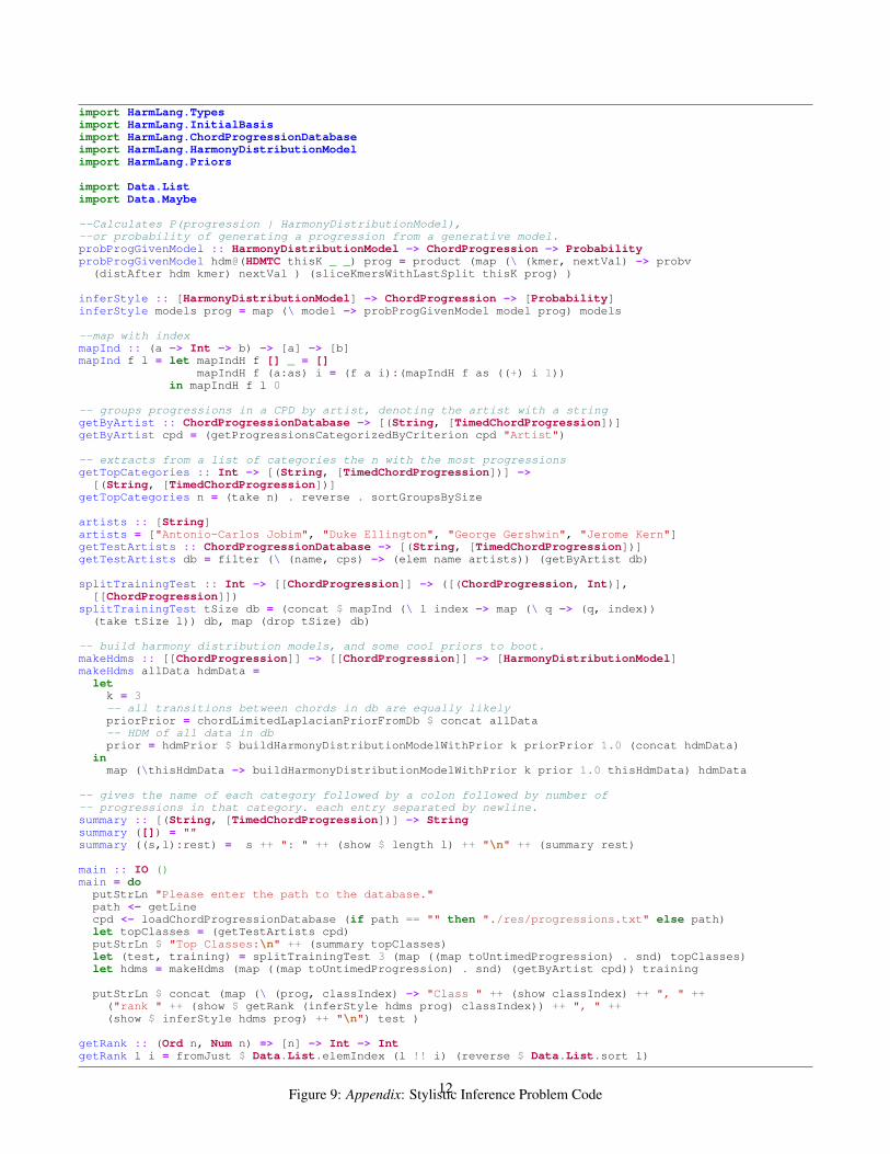
The full code for the stylistic inference problem is available in the appendix, figure A9, but the majority of it is boilerplate6
and IO. We were able to express the inference code itself in a tiny amount of code, which speaks to the success of the languagein simplicity and brevity. The relevant code appears in Figure 3.
The core of the stylistic inference problem is quick to implement using the core abstractions offered by HarmLang, asdemonstrated in Figure 3. It works by building a HarmonyDistributionModel for each composer, using the prior dis-cussed in Section 1.5.3 and the training data for the specific composer. This amounts to loading up the Markov states (chordsequences of length 3) with transition probabilities reflecting the changes seen in the composer’s corpus of music. As theHarmonyDistributionModel is essentially a Markov chain, it is easy to ask the question ”what is the probability thatthis HDM generated this chord progression?” Given a song that was not used in the training data, we ask this question of eachof the composer-specific models and compare the results. We say the model that is most likely to have generated the given songcorresponds to the most likely composer of that song.
HarmLang saved us both from having to write a parser for the input data and from having to write a conditional probabilitysystem, and additionally we benefited from HarmLang’s domain specific optimizations, such as the Key Agnosticism Property(Section 1.5.2). We were able to express a very complicated program in a very concise amount of code (see Figure 3, soHarmLang is useful at least for probabilistic applications such as this.
3 Beyond HarmLang: A Generalization of Conditional Probability Techniques
3.1 Generalizing the Key Agnosticism Property3.1.1 A motivating example
In this section we present a similar probabilistic problem and examine Key Agnosticism from a different angle to motivateits generalization.
The Highway Problem Suppose we have images of intersections with labeled cars and labeled trajectories of a speciallylabeled car (See Figure 5). We wish to use this information to predict what direction cars will turn when they reach anintersection, based on their location relative to other cars.
The data we are trying to extract is the heading after the special car navigates the intersection, and the evidence is theintersection itself: but the space of intersection images is far too vast to condition over. We need a way of reducing theinformation in our evidence for our conditional distributions, but we also need a way of retrieving some of this evidence after
6At present, it is a bit more difficult than we would like to operate on a HDM, and priors are more difficult to work with than we would like, though thereis a simpler build function for those who wish to use an HDM without a prior that is much easier to use.
6
a query is made. We want to form conditional distributions over this evidence and data type; these conditional distributionsshould have type Intersection -> Dist Direction.
In our evidence reduction step, we want to rotate an intersection so that the labeled car begins at the top of the intersection, sowe may consider intersections where cars begin at different locations to be equivalent, and condition on more useful information,such as the locations of nearby vehicles and the size of the vehicle in question. We also want to discretize the positions of cars,because shrinking the evidence space reduces the amount of data required to build a useful model, and this discretization stepwill allow us to have a finite evidence space.
Now, we can apply the evidence reduction step to each intersection instance used to build the intersection model, and we areleft with a set of discretized intersections where the special car is at the top of the intersection. All this is analogous to the stepof transposing every sequence of chords to begin on A (in stylistic inference, the evidence is a set-length sequence of chords andthe data are chords that might follow. In the Highway Problem, the data is the heading that the car ended up on after a certainintersection state. Our evidence reduction step applied some rotation to the intersection, and our data is a heading in the contextof the original rotation: we must apply the same rotation to the data heading that we did to the evidence intersection. Nowwe can use these transformed evidence data pairs to build a conditional distribution using the conditional distribution factorycombinator discussed in Section 1.4.2.
One question remains: we have built a conditional distribution of rotated intersections onto rotated headings, but how dowe use it with an unrotated intersection? The straightforward answer is to rotate an intersection and then make a query, so wetransform query evidence in the same manner that we transform training evidence. But now, a new problem arises: to answerquestions about the direction a car will go, we must transform the rotated data obtained from a query to the rotated conditionaldistribution into unrotated data that matches the raw, unrotated evidence.
In the construction phase we needed to create a function that rotated the turn direction data into the rotated space, but herewe must have a function that rotates rotated directional data into the unrotated space. We thus use the inverse of the rotationused to convert the evidence to the unrotated space, and apply this rotation to the data distribution resulting from the query onthe distribution (this conversion can be accomplished using pmap on the rotated distribution with the antirotation function).
Now we have an inner conditional distribution, which takes evidence in the rotated evidence space, which we shall denoteevidence’, and maps it onto data in the rotated data space, which we shall denote data’. We also have a method of convertingevidence to evidence’, and a method of converting data’ distributions back to data distributions. We can thus “wrap” this innerdistribution (of type evidence’ -> Dist data’) in an outer distribution of type evidence -> Dist data, whichis exactly the type of an ordinary conditional distribution!
To recap, in model creation, we needed a function that took evidence onto a possibly – but not necessarily – reduced space,evidence’, but this function also needed to take data onto a data’ space. This function would have type evidence -> data-> (evidence’, data’). In model queries, we needed a function that took evidence onto the rotated space, and alsoproduced an inverse rotation function to pmap over the data. This function takes the form evidence -> (evidence’,data’ -> data. With some careful rearranging, we can combine these functions into one function, which we name thetransformer creator function, of type evidence -> (evidence’, data -> data’, data’ -> data). Thiscombined function takes some evidence, produces the transformed (rotated) evidence, and gives a function to convert datainto the transformed space, and finally gives a function to convert data back out of the transformed space. The function containsinformation that defines how the internal representation in one of these HDM-esque models differs from the external queriesand answers that are seen by clients.
3.1.2 Key Agnosticism in the Generalized Model
We can rephrase key agnosticism in the context of a more general model, similar to the example given in the HighwayProblem. Here we discuss what such a reorganization entails, and some of the subtler benefits of doing so.
In HarmLang, our evidence is of the form [Chord], and our data distributions are of type Chord. Both evidence andevidence’ have the same type, and data and data’ are of the same type as well, so the HarmLang use is actually a special case ofa more general concept. The evidence transform simply takes a chord progression and transposes it such that the first chord ofthe progression is rooted at A. Denote the interval by which to transpose i, and we must transpose the data (which representsthe chord after the progression) by i as well to put it into the “rotated” space. Thus our data transformer is simply transposei. Finally we need to provide a data antitransformer, which must simply be the inverse transpose, or transpose (inversei).
In doing so, we have created a function that given evidence, produces the requisite transformed evidence, and providestransformers between the data and data’ spaces. In the development of HarmLang, we considered representing Chords as
7
type ConditionalDist ev dat = ev -> Dist dat
type Transformer ev ev’ dat dat’ = ev -> (ev’, dat -> dat’, dat’ -> dat)
buildTransformedConditionalDist ::(Ord ev, Ord ev’, Eq dat, Eq dat’) => Transformer ev ev’ dat dat’ -> [(ev, dat)] -> ConditionalDist ev dat
buildTransformedConditionalDist t dat =let toInner (ev, dat) = let (innerEv, dTrans, _) = t ev in (innerEv, dTrans dat)
innerDist = buildConditionalDist $ map toInner datouterDist e = let (innerE, _, dInvTrans) = t e in pmap dInvTrans (innerDist innerE)
in outerDist
Figure 6: Haskell Code for Transformer Antitransformer Combinators
integers, using a mapping based on their finite enumeration (discussed in Section 1.3). This representation would be quite aperformance enhancement, both in terms of memory used and speed of comparison for CHORDs, and so is quite advantageousin practice. Using the Transformer Antitransformer Paradigm, we can actually implement this, by making the evidence’ type be[Int], and the data’ type be Int. The inner types are thus represented as integers, and the expensive distribution constructionoperations (and any other probabilistic operations) happen on distributions of simple integers, but these inner types are invisibleto the end user, who only sees the outer distribution types ([Chord] and Chord) exposed.
Here we see that in addition to transforming evidence to reduce the evidence space, we can also compress our representationof evidence and data to yield faster computations.
3.1.3 The Transformer Antitransformer Paradigm
We have now seen the key ideas at work in both the Highway Problem and the Key Agnosticism Problem, and we are readyto formalize them and create combinators to produce conditional distributions using these transformers.
In order to build a transformed conditional distribution, we require our evidence data pairs (as in construction of a nor-mal conditional distribution, discussed in Section 1.4.2), and we also need a Transformer, which is simply a evidence-> (evidence’, data -> data’, data’ -> data) function. This function abstracts all of the logic requiredto transform evidence to the inner evidence space, and data between the inner and outer data spaces. The Haskell code forbuildTransformedConditionalDist can be found in Figure 6.
In addition to these types, we also require that for any Transformer object t, for any evidence e and any data d, ifwe let (e′, dTrans, dAntiTrans) = te, then d = dAntiTrans . dTrans d. We want the antitransformer to be aninverse of the transformer to guarantee that data information conversion is lossless: it may be compressed or converted intoa different format, will not be transformed into some form such that the antitransformer can not recover the original. Theauthors note that pmap provides a fine way to perform lossy conversions over data, and, like all functions over distributions,is also compatible with conditional distributions, as discussed in Section 1.4.2. We denote this property the inverse property ofconditional transformers.
Given this requirement, we now prove the following simple but highly useful result:
Result 1. For any evidence, the space of possible data in a conditional distribution is the same as the space of possible data ina transformed conditional distribution.
Proof. Suppose we are given some e ∈ evidence and some d ∈ data. We wish to show that for this evidence, this d, which isarbitrary, can have support in the transformed distribution. In fact, we will show that it can even be certain in the distribution:suppose the transformed conditional distribution were created using only [(e, d)] as evidence for some transformer t. Then eis mapped onto some e′ ∈ evidence’, and d onto some d′ ∈ data’ in the inner distribution. Since this is the only data, it hasprobability 1 in the inner conditional distribution for evidence e′. Now, since e maps to e′ by the transformer, and d′ mustmap back to d by the antitransformer, because of the inverse property of conditional transformers, we have that in the outerconditional distribution, e maps to a distribution where d is certain. Thus for any e, d in evidence, data, respectively, d mayhave nonzero probability in the transformed distribution.
And now, as promised, is a proof of the key agnosticism property.
8
Result 2. Transformed conditional distributions created with transformer described in Section 3.1.2 have the Key AgnosticismProperty.
Proof. Suppose we have some evidence of type ChordProgression a, and some arbitrary interval b. When we query thetransformed conditional distribution d with a, it is converted to the key of A so transposed by some interval ai, and the resultingdistribution is transposed by inverse ai. We then transpose the distribution7 by b. These steps represent the expression“transpose b (d a)”. We note that this is equivalent the distribution produced by “d (transpose b a)”, because thisdistribution is produced by querying the inner distribution after transposing transpose b a by ai+ inverse b (to reachthe key of A), and then this is undone in the inverse transform, which means that the resulting distribution is transposed byinverse (ai+ inverse b) = (inverse ai) + b. We had the exact same inner distribution, and applied the inverse aitransposition, as well as the b transposition, in the conversion to the outer distribution: in the previous expression, we did theexact same thing, only the b transposition was because of the definition of the key agnosticism property. We thus have that withthis transformer, for any evidence a and interval b, transpose b (d a) = d (transpose b a).
4 Conclusion
4.1 Further WorkIn a recent presentation on HarmLang, Avi Pfeffer suggested that we use a multi-tiered distribution approach for chords,
where subsequent distributions discard more and more information as we move from tier to tier. This idea does not fit into theTransformer Antitransformer Paradigm discussed in this paper because we are actually discarding data information in it, but itdoes seem like it would be very effective in practice for the types of problems we want to solve using HarmLang. Currently weare using very large priors, but the multi tiered distribution tactic seems like an effective alternative.
Norman Ramsey suggested that we use to use lower order Markov Models in conjunction with a full k order model, andweight the evidence from each model by its k value and the number of instances of training information that went in eachone. This is also a very interesting potential direction, and like the key agnosticism transformer discussed in this paper, it alsoworks by shrinking evidence spaces (evidence is a smaller chord array in a lower order model), although it doesn’t fit into theTransformer Antitransformer Paradigm either.
We wish to pursue both these avenues in further HarmLang development, and we also wish to solve more probabilisticproblems with HarmLang. One such problem is the chord recognition problem where given an audio stream, we assume that itwas produced by a Hidden Markov Model (Baum and Petrie 1966), the HMM being some trained model that we provide, andwe attempt to recover the state transitions that led to the production of the audio stream. Chord Progression Recognition is abig problem in Music Information Retreival (Yu et al. 2012), and is a necessary first step in any MIR if we wish to subsequentlyrun the Stylistic Inference algorithm presented here to detect styles or artists.
4.2 ContributionsIn this paper, we present a language for probabilistic inference over chord progressions, and show results of an example
inference problem. We also present the domain specific Key Agnosticism Property, and discuss the use of various priors that weexperimented with.
In addition to the HarmLang specific work we have done, we have defined a basic constructor for a conditional probabil-ity distribution, of type [(evidence, data)] -> (evidence -> Dist data)], and showed that when evidenceis of type [data], Markov models can be converted into the form used by this constructor, the conversion being of type[[data]] -> [([data], data)]. We also created the Transformer Antitransformer Paradigm, in which the user pro-vides a function that given evidence, normalizes and possibly reduces the evidence into a new space, and creates transformersthat perform similar normalization on data and undo said normalization, and showed several uses and valuable properties of con-ditional distributions created in this manner (conditional distributions created in this manner are called transformed conditionaldistributions by some transformer).
4.3 AcknowledgementsNorman Ramsey for his work on the Probability monad, and his lectures on the largely isomorphic Dice World finite
discrete probability system that many of the probabilistic aspects of HarmLang were based on.
7Transposition of a distribution of chords d by interval i is simply defined by pmapping the transpose i over d.
9
Avi Pfeffer for his feedback and suggestions on ways to improve the use of training data in HarmLang.Kathleen Fisher for educating us in language design, Haskell, and the tools necessary to build an embedded language.Louis Rassaby for tirelessly laboring on the nonprobabilistic parts of the HarmLang language.
ReferencesLeonard E. Baum and Ted Petrie. Statistical inference for probabilistic functions of finite state markov chains. Ann. Math.
David Cope. Computer models of musical creativity. MIT Press Cambridge, 2005.
Pedro J Ponce De Leon, Carlos Perez-Sancho, and Jose M Inesta. A shallow description framework for musical style recogni-tion. In Structural, Syntactic, and Statistical Pattern Recognition, pages 876–884. Springer, 2004.
Paul Hudak. The Haskell School of Music – From Signals to Symphonies. (Version 2.6), January 2014.
AA Markov. Rasprostranenie zakona bol’shih chisel na velichiny, zavisyaschie drug ot druga. izv fiz-matem obsch kazan univ(series 2) 15: 135–156. see also:“extension of the limit theorems of probability theory to a sum of variables connected in achain”. Appendix B of R. Howard “Dynamic Probabilistic Systems, 1, 1906.
Ralph Patt. The Vanilla Book. http://www.ralphpatt.com/VBook.html, August 2014.
Norman Ramsey and Avi Pfeffer. Stochastic lambda calculus and monads of probability distributions. ACM SIGPLAN Notices,37(1):154–165, 2002.
Claude E Shannon. Prediction and entropy of printed english. Bell system technical journal, 30(1):50–64, 1951.
M. Stone. Cross-validatory choice and assessment of statistical predictions. J. Royal Stat. Soc., 36(2):111–147, 1974.
Yi Yu, Roger Zimmermann, Ye Wang, and Vincent Oria. Recognition and summarization of chord progressions and theirapplication to music information retrieval. In Proceedings of the 2012 IEEE International Symposium on Multimedia, ISM’12, pages 9–16, Washington, DC, USA, 2012. IEEE Computer Society. ISBN 978-0-7695-4875-3. doi: 10.1109/ISM.2012.10. URL http://dx.doi.org/10.1109/ISM.2012.10.
-- equivalent to Ramsey’s monadic return in PMonad.hscertainly :: (Eq a) => a -> Dist a-- equivalent to choose in the probability monadchoose :: (Eq a) => Double -> Dist a -> Dist a -> Dist aequally :: (Eq a) => [a] -> Dist aweightedly :: (Eq a) => [(a, Double)] -> Dist a
Transformers:
pmap :: (Eq a, Eq b) => (a -> b) -> Dist a -> Dist b-- equivalent to (>>=) in the probability monadbind :: (Eq a, Eq b) => Dist a -> (a -> Dist b) -> Dist bpfilter :: (Eq a) => (a -> Bool) -> Dist a -> Dist a
Observers:
-- Probability of a value in a distribution.probv :: (Eq a) => Dist a -> a -> Double-- Prob of seeing a value that matches a given predicateprob :: (Eq a) => (a -> Bool) -> Dist a -> Double-- Expectation of a function over the distributionexpected :: (Eq a) => (a -> Double) -> Dist a -> Double-- Returns all a with nonzero probability in the distributionsupport :: Dist a -> [a]-- Gives a list of values paired with the probs, sortedlikelylist :: Dist a -> [(a, Double)]-- Returns the most likely a in the distribution.maxlikelihood (Eq a) -> Dist a -> a
Figure 7: Appendix: Functions to operate on distributions. Inspiration drawn from (Ramsey and Pfeffer 2002).
Classes 0 through 3 and number of songs for each:Jerome Kern: 13George Gershwin: 16Antonio-Carlos Jobim: 10Duke Ellington: 13
Song belonging to class 0; class 0 ranked #1 most likely to generate:[1.4059454075968913e-13,9.540545701315283e-25,3.6240722125929777e-28,1.0604786997127541e-28]
Song belonging to class 0; class 0 ranked #1 most likely to generate:[2.506780001598519e-65,7.528215296946187e-72,7.2147257457420656e-68,1.0386318614385804e-69]
Song belonging to class 0; class 0 ranked #1 most likely to generate:[2.9798618616567765e-72,lsˆ?ˆ?1.59576879617857e-75,2.2639725582290817e-74,1.9602214375292068e-74]
Song belonging to class 1; class 1 ranked #1 most likely to generate:[5.61153953481877e-105,2.5857909175756105e-98,1.7696122136215285e-98,1.2924084332183754e-102]
Song belonging to class 1; class 1 ranked #3 most likely to generate:[5.981763636760707e-60,6.986251472717658e-62,3.36590976019944e-59,6.79726803315224e-62]
Song belonging to class 1; class 1 ranked #4 most likely to generate:[3.7902683346153304e-119,3.208655678645729e-126,2.14300934701038e-117,6.003209926431248e-121]
Song belonging to class 2; class 2 ranked #2 most likely to generate:[5.146214982802794e-48,1.6975665796000584e-48,2.7813307594515686e-47,3.1223325738092487e-47]
Song belonging to class 2; class 2 ranked #1 most likely to generate:[3.546151149341456e-171,2.8736089568265408e-173,2.3291381786128676e-168,2.6655259881872177e-171]
Song belonging to class 2; class 2 ranked #1 most likely to generate:[8.817143090881416e-94,2.862164432778404e-93,1.7274675688951576e-91,3.999357088630745e-95]
Song belonging to class 3; class 3 ranked #2 most likely to generate:[3.5855991986422204e-76,6.976010084269398e-77,1.0215705963472741e-73,2.658516275402443e-74]
Song belonging to class 3; class 3 ranked #4 most likely to generate:[8.330491071734757e-18,8.994654612974338e-22,2.0277753754750986e-21,7.301698190061534e-23]
Song belonging to class 3; class 3 ranked #4 most likely to generate:[1.4966626836963026e-73,7.52740659436434e-78,7.079525901999664e-75,1.8217099178619128e-79]
Figure 8: Appendix: Raw output from our stylisticinference program. The printed lists include, in order, the proba-bilities that each composer’s HarmonyDistributionModel would generate the song in question.
--Calculates P(progression | HarmonyDistributionModel),--or probability of generating a progression from a generative model.probProgGivenModel :: HarmonyDistributionModel -> ChordProgression -> ProbabilityprobProgGivenModel hdm@(HDMTC thisK _ _) prog = product (map (\ (kmer, nextVal) -> probv(distAfter hdm kmer) nextVal ) (sliceKmersWithLastSplit thisK prog) )
inferStyle :: [HarmonyDistributionModel] -> ChordProgression -> [Probability]inferStyle models prog = map (\ model -> probProgGivenModel model prog) models
--map with indexmapInd :: (a -> Int -> b) -> [a] -> [b]mapInd f l = let mapIndH f [] _ = []
mapIndH f (a:as) i = (f a i):(mapIndH f as ((+) i 1))in mapIndH f l 0
-- groups progressions in a CPD by artist, denoting the artist with a stringgetByArtist :: ChordProgressionDatabase -> [(String, [TimedChordProgression])]getByArtist cpd = (getProgressionsCategorizedByCriterion cpd "Artist")
-- extracts from a list of categories the n with the most progressionsgetTopCategories :: Int -> [(String, [TimedChordProgression])] ->[(String, [TimedChordProgression])]
getTopCategories n = (take n) . reverse . sortGroupsBySize
splitTrainingTest :: Int -> [[ChordProgression]] -> ([(ChordProgression, Int)],[[ChordProgression]])
splitTrainingTest tSize db = (concat $ mapInd (\ l index -> map (\ q -> (q, index))(take tSize l)) db, map (drop tSize) db)
-- build harmony distribution models, and some cool priors to boot.makeHdms :: [[ChordProgression]] -> [[ChordProgression]] -> [HarmonyDistributionModel]makeHdms allData hdmData =
letk = 3-- all transitions between chords in db are equally likelypriorPrior = chordLimitedLaplacianPriorFromDb $ concat allData-- HDM of all data in dbprior = hdmPrior $ buildHarmonyDistributionModelWithPrior k priorPrior 1.0 (concat hdmData)
inmap (\thisHdmData -> buildHarmonyDistributionModelWithPrior k prior 1.0 thisHdmData) hdmData
-- gives the name of each category followed by a colon followed by number of-- progressions in that category. each entry separated by newline.summary :: [(String, [TimedChordProgression])] -> Stringsummary ([]) = ""summary ((s,l):rest) = s ++ ": " ++ (show $ length l) ++ "\n" ++ (summary rest)
main :: IO ()main = doputStrLn "Please enter the path to the database."path <- getLinecpd <- loadChordProgressionDatabase (if path == "" then "./res/progressions.txt" else path)let topClasses = (getTestArtists cpd)putStrLn $ "Top Classes:\n" ++ (summary topClasses)let (test, training) = splitTrainingTest 3 (map ((map toUntimedProgression) . snd) topClasses)let hdms = makeHdms (map ((map toUntimedProgression) . snd) (getByArtist cpd)) training