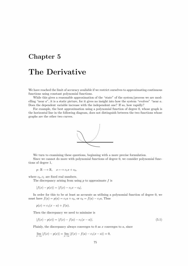
i Mathematics today is a vast enterprise. Advances and breakthroughs have been painstakingly built on the structure(s) erected by earlier mathematicians. The history of mathematics is quite different from the that of other human endeavours. In other fields, previously held views are typically extended or proved wrong with each advance – there is a process of correction and extension. “Only in mathematics is there no significant correction – only extension”. The work of Euclid has certainly been extended many times. Euclid, however, has not been corrected – his theorems are valid today and for all time! The other remarkable thing about mathematics is its extraordinary utility in describing and quantifying the world around us. Mathematics is the language of the sciences, both natural and social. This forces mathematics to be abstract, since it must embrace theories from physics, economics, chemistry, psychology, etc. Mathematics is so widely applicable precisely because of — not despite — its intrinsic abstractness. MATH101 is the first half of the MATH101/102 sequence, which lays the foundation for all further study and application of mathematics and statistics, presenting an introduction to dif- ferential calculus, integral calculus, algebra, differential equations and statistics, providing sound mathematical foundations for further studies not only in mathematics and statistics, but also in the natural and social sciences. Achieving this, requires a brief, preliminary foray into the basics of mathematics, because much of the material requires a high degree of abstract reasoning, rather than rote learning of computational techniques. A rigorous approach to the basics provides a deeper understanding of the whole structure. The assumptions upon which the structure is built are thereby clarified, with both the scope and limitations of the intellectual framework made readily understandable. Moreover, this deeper understanding, does not come at the expense of applicability. Quite the contrary! One consequence of providing sound fundamentals is that there is considerable time devoted to matters whose importance and applicability is not immediately obvious. But such study of these fundamental areas of mathematics is also stimulating. If you enjoy puzzles here is an “intellectual game” par excellence. A game played within a rigid framework of rules, but with unlimited scope for creativity in the search for problems and the solutions to problems. The genesis of theses notes is the set of notes originally prepared for MATH101 by Chris Radford, with the help of Margaret McDonald, Robyn Curry and Meg Vivers in typsetting these notes. Later, Gerd Schmalz revised them, making additions and significant improvements. I incorporated their ideas and insights, as well as comments from students and colleagues, into these notes, when adapting the notes. Bea Bleile has been generous with her time, comments and suggestions. Her ruthless honesty is appreciated and has spared the reader some headaches. All remaining mistakes, errors and infelicities of style are mine alone. The reader is invited and encouraged to point out any mistakes (s)hefinds. I hope the reader enjoys the challenges the course offers, and that (s)he experiences a sense of achievement at the end. I. Bokor December, 2010
Transcript
i
Mathematics today is a vast enterprise. Advances and breakthroughs have been painstakinglybuilt on the structure(s) erected by earlier mathematicians.
The history of mathematics is quite different from the that of other human endeavours. In otherfields, previously held views are typically extended or proved wrong with each advance – there isa process of correction and extension. “Only in mathematics is there no significant correction –only extension”.
The work of Euclid has certainly been extended many times. Euclid, however, has not beencorrected – his theorems are valid today and for all time!
The other remarkable thing about mathematics is its extraordinary utility in describing andquantifying the world around us. Mathematics is the language of the sciences, both natural andsocial. This forces mathematics to be abstract, since it must embrace theories from physics,economics, chemistry, psychology, etc. Mathematics is so widely applicable precisely because of— not despite — its intrinsic abstractness.
MATH101 is the first half of the MATH101/102 sequence, which lays the foundation for allfurther study and application of mathematics and statistics, presenting an introduction to dif-ferential calculus, integral calculus, algebra, differential equations and statistics, providing soundmathematical foundations for further studies not only in mathematics and statistics, but also inthe natural and social sciences.
Achieving this, requires a brief, preliminary foray into the basics of mathematics, becausemuch of the material requires a high degree of abstract reasoning, rather than rote learning ofcomputational techniques.
A rigorous approach to the basics provides a deeper understanding of the whole structure.The assumptions upon which the structure is built are thereby clarified, with both the scopeand limitations of the intellectual framework made readily understandable. Moreover, this deeperunderstanding, does not come at the expense of applicability. Quite the contrary!
One consequence of providing sound fundamentals is that there is considerable time devoted tomatters whose importance and applicability is not immediately obvious. But such study of thesefundamental areas of mathematics is also stimulating. If you enjoy puzzles here is an “intellectualgame” par excellence. A game played within a rigid framework of rules, but with unlimited scopefor creativity in the search for problems and the solutions to problems.
The genesis of theses notes is the set of notes originally prepared for MATH101 by ChrisRadford, with the help of Margaret McDonald, Robyn Curry and Meg Vivers in typsetting thesenotes. Later, Gerd Schmalz revised them, making additions and significant improvements. Iincorporated their ideas and insights, as well as comments from students and colleagues, intothese notes, when adapting the notes. Bea Bleile has been generous with her time, comments andsuggestions. Her ruthless honesty is appreciated and has spared the reader some headaches.
All remaining mistakes, errors and infelicities of style are mine alone. The reader is invitedand encouraged to point out any mistakes (s)hefinds.
I hope the reader enjoys the challenges the course offers, and that (s)he experiences a sense ofachievement at the end.
“The essence of mathematics lies in its freedom”, wrote Georg Cantor, the great mathe-matician. This freedom should be made visible in elementary and high-school classes. Thisis not to be had without formal stringency, and not without concentrated learning.
— Gero von Randow ([?] p.4)
Chapter 0
Introduction
Only a minority of those who study mathematics do so out of interest in mathematics itself. Moststudents take mathematics because it is needed for their main interest, commonly for modellingphenomena, processes or complex systems in the natural sciences, engineering, economics or else-where. Mathematical models are needed to make possible testable predictions and for theoreticalunderstanding.
Making testable predictions means that mathematical models need to satisfy two requirements.
1. They must be accurate.
2. They must be computable.
These two requirements are antagonistic. Developing mathematic models is, therefore, a deli-cate optimisation problem:
Construct a mathematical model accurate enough to be dependable, while computableeasily enough to be usable.
Both the difficulty and the importance of this task is illustrated by the “climate change debate”.
The aims of these notes include providing an introduction to, and induction in, mathematicalmodelling. They provide only the very first steps in rudimentary mathematical modelling. Onlysome of the most basic tools and elementary concepts, tools and techniques are introduced here.But these provide the basis for the development of more sophisticated and powerful techniques.
A science is an organised body of knowledge. A crude sketch of the evolution of science andscientific technique is that it began with observation of the world around us and the accumulationof empirical data. But a collection of facts is not yet knowledge — if it were, a current telephonedirectory would be an encyclopædia. The urge to understand led to embedding observations intotheory to explain the data. This requires clear and precise formulation of the necessary conceptsand procedures, especially mathematical ones.
Experience prompted conjectures concerning the relationship between observed phenomena ormeasured quantities, such as variation in one causing variation in another in some fixed manner.
The following examples may clarify this.
1 Given a fixed volume of a gas in a rigid, undeformable container, it can be observed the thepressure of the gas rises with the temperature. This was investigated in controlled experiment,varying one measurable quantity, say pressure, and observing the changes in the other measurablequantity, temperature. By ensuring that the ambient conditions were replicated, such experimentscould be repeated, or duplicated, at different times in different places. Typically, the data ispresented in graphical form, with one of the observables represented by the horizontal axis andthe other by the vertical axis.
1
2 CHAPTER 0. INTRODUCTION
•
•
•
•
•
We usually regard one variable, say u, as a function of the other, say t, and we therefore seeka function, “u = f(t)”, whose graph passes through the given points. We use calculus when theprocess we model by our function is a continuous process.
2 Centuries after smoking tobacco became common in Western societies, it was observed thatcertain diseases, especially cancers, seemed to afflict smokers more frequently than non-smokers,resulting in premature mortality. In this case, it is not possible to replicate observation, orduplicate the precise conditions. Instead, the nature of any relationship between smoking andpremature mortality needs to be deduced from unrepeatable observations of different subjects.Such data can also be depicted diagrammatically.
•
•••
••
•
•••
•
•
••
••
•
•
•
In such cases, we use statistics to determine the extent to which the observable are related,and nature of such a relationship.
In this course, we concentrate on the first kind of problem and the mathematics we developreflects this. This does not mean that we neglect the latter kind of problem, for statistics is basedon and uses the mathematics we develop here.
Our problem then, can be formulated more preciely.
1. Find a real valued function of a real variable, whose graph passes through the givenpoints.
2. When there isn’t one, find the “nearest” one.
3. When there is more than one, determine the “best” one.
This provides the leitmotif for these notes. The theory and techniques we develop can befruitfully thought of as a project aimed at solving this problem.
A remarkable feature of the theory and techniques we develop is that their range of applicabilityextends far beyond our specific problem.
Consequently, we take time and care to develop the ideas and techniques in general form.These notes do not simply comprise a compendium of formulæ and tricks to be copied “monkeysee, monkey do” fashion.
This generality is not for its own sake. Rather, it highlights and places into perspective, theessential ideas. Moreover, it is indispensable for the advance of science, as Paul Dirac observed in1931.
3
The steady progress of physics requires for its theoretical formulation a mathematics thatgets continually more advanced. This is only natural and to be expected. What howeverwas not expected by the scientific workers of the last century was the particular form thatthe line of advancement of the mathematics would take, namely, it was expected that themathematics would get more and more complicated, but would rest on a permanent basisof axioms and definitions, while actually the modern physical developments have required amathematics that continually shifts its foundations and gets more abstract. Non-euclideangeometry and non-commutative algebra, which were at one time considered to be purelyfictions of the minds and pastimes of logical thinkers, have now been found to be verynecessary for the description of general facts of the physical world. It seems likely thatthis process of increasing abstraction will continue in the future and that advances inphysics is to be associated with a continual modification of the axioms at the base ofmathematics rather than with a logical development of any one mathematical scheme ona fixed foundation.
The Structure of These Notes
We are interested in mathematical modelling using real valued functions of a real variable. Thisrequires an understanding of general mathematical principles, the language of mathematics, theproperties and structure of the real numbers and of functions.
The first and foremost principles are that mathematics needs to be expressed precisely andthat mathematical arguments need to be sound and reliable. To ensure we achieve this, we beginwith a brief account of the logic we use. Proof is indispensable to mathematics, for a proof is acomplete explanation and justification, taking care of any potential “what if . . . ?”
The mathematics we develop is expressed in terms of sets and functions between sets. Wediscuss sets and operations on sets before turning to the most familiar sets — natural numbers,whole numbers, rational numbers and real numbers.
We revise the arithmetic operations on them, as well as their usual ordering. We formulate thebasic rules governing these in the form of axioms and show how other rules familiar to the readercan be deduced from these. In other words, we formulate arithmetic algebraically.
We then discuss functions between sets, first in general, and then in the particular cases ofgreatest interest to us. The axiomatic formulation of arithmetic is immediately put to use byshowing that functions taking real numbers as values behave almost identically to real numbers.Indeed, we regard the set of all functions defined on a fixed set, X, and taking only real numbersas values, as a generalisation of the set of all real numbers, and we can calculate with them inalmost the same manner. The axiomatic formulation tells us the pitfalls and when they occur.
These preliminary discussions serve to revise earlier material, summarise it in rigorous form,to introduce and fix concepts and notation, all in a modern, mathematical manner.
We then return to our problem. Our strategy is to focus on each individual point first, seekinga suitable curve at each point, with the intention of then splicing these partial curves together.
To meet the (mutually antagonistic) requirements for mathematical models, we choose to usepolynomial functions. Their values can be computed using finitely many elementary arithmeticoperations. We use the degree of such polynomial functions as a measure of their complexity.
We begin with polynomial functions of degree 0, which are constant functions, as these are theleast complex ones. The requirement that these provide a usable approximation leads naturallyto the notions of limit and continuity.
We investigate the relationship between the notion of limit and the algebraic operations onreal valued functions of a real variable and see that it is enough to know the limits of four basicfunctions in order to be able to compute limits for the functions used in most applications. Thisprovides an algorithm for computing limits for such functions.
We investigate continuous functions and discover they have many convenient properties, whichallow us to draw some powerful conclusions, including the Intermediate and Mean Value Theorems.
4 CHAPTER 0. INTRODUCTION
The limitations arising from the restriction to polynomial functions of degree 0 — the sim-plest ones — soon become apparent from concrete examples. In response, we increase make theminimum increase in complexity by considering polynomial functions of degree at most 1. We for-mulate an intuitive notion of the best approximation using such functions, which naturally yieldsthe definition of the derivative and differentiability. Rather satisfactorily, we find that a functionhas a (unique!) best approximation at a point if and only if it is differentiable at that point.
As in the case of continuity, we investigate the relationship between differentiation and thealgebraic operations on real valued functions of a real variable, and find that it is enough toknow he derivatives of the same four basic functions in order to be able to compute limits for thefunctions used in most applications. This provides an algorithm for computing the derivatives ofsuch functions.
We also see that by iterating the process of differentiation, we obtain more information aboutthe shape of the graph of the function in question. We provide examples, illustrating this for avariety of functions, emphasising the most commonly occurring ones..
These developments also raise practical problems. For example, we frequently need to findwhere a given function takes particular value. While there is no general solution to this problem,our theory provides a powerful method, the Newton-Raphson Method for solving such problemsalgorithmically under some mild constraints.
We also present a uniform method for approximating “sufficiently smooth” functions to anydegree of accuracy, using functions whose values are readily computed, namely Taylor polynomials.
Finally, we return to purely algebraic considerations arising when we try to solve several simpleequations — linear equations — simultaneously. This theory is probably the most comon appli-cation of matematics. We see that the algebraic properties generalise those of the real numbers.
We also investigate another generalisation of central importance to the natural sciences, engi-neering and geometry, namely vectors, and their algebraic properties.
Chapter 1
Notation, Logic and Proof
1.1 The Greek Alphabet
The Greek alphabet is frequently used in the mathematical sciences. We list its characters andtheir names for the benefit of those who are not yet familiar with them.
Mathematics concerns itself with statements, or, more particularly, relationships between state-ments. Bertand Russell characterised mathematics as being the study of which statements followlogically from which statements. This places proof at the centre of mathematics.
We therefore begin with the logic we use. Since a complete, rigorous account would distractus too much from our principal aims, we only provide a brief summary here. A comprehensiveaccount can be found in I.M.Copi’s Symbolic Logic.
5
6 CHAPTER 1. NOTATION, LOGIC AND PROOF
Definition 1.1. A proposition or statement is any sentence about which it can be sensibly saidthat it is true.
A proposition is compound when it contains another proposition. Otherwise it is simple.
Example 1.2. We illustrate the above.
(i) Wash your hands before eating.
This is not a proposition (statement). It is an imperative.
(ii) What time does the next bus to town leave?
This is not a proposition (statement). It is a question.
(iii) Columbus discovered America.
This is a simple proposition.
(iv) All swans are white and some ducks are white.
This is a compound proposition, the conjunction of the two simple propositionsAll swans are white.
andSome ducks are white.
(v) The moon is not made of green cheese.
This is a compound proposition, the negation of the simple propositionThe moon is made of green cheese.
(vi) This cheese is Australian or it is imported.
This is a compound proposition, the disjunction of the two simple propositionsThis cheese is Australian.
andIt (this cheese) is imported.
(vii) If woollen clothes are washed in hot water, then they shrink.
This is a compound proposition, the conditonal of the two simple propositions, the an-tecedent ,
Woollen clothes are washed in hot water.and the consequent ,
They (woollen clothes) shrink.
(viii) The integer, n, is even if and only if there is a remainder of 0 on division by 2.
This is a compound proposition, the biconditonal of the two simple propositionsThe integer, n, is even .
andThere is a remainder of 0 on division by 2..
Remark 1.3. The word “or” is ambiguous in everyday language.“P or Q”, is sometimes used in an exclusive sense, so that “P or Q” is true whenever one and
only one the statements P , Q, is true, Read this asOne, or other, but not both.
At other times, jt is used in an inclusive sense so that “P or Q” is true at least one a thestatements P , Q, is true.
Read this asOne, or other, and possibly both.
Standard practice in logic is to use the disjunction in the broader, inclusive sense, explicitlyspecfiying “exclusive or” on those occasions when that is intended. We follow this standard practicehere.
1.2. LOGIC AND PROOF 7
Notation 1.4. If P and Q are propositions, we often write
1. ¬P for the negation of P : not P ,
2. P ∨Q for the disjunction of P and Q: P or Q,
3. P ∧Q for the conjunction of P and Q: P and Q,
4. P ⇒ Q for the conditional with antecedent P and consequent Q: If P , then Q
5. P ⇔ Q for the biconditional of P and Q: P if and only if Q
Remark 1.5. For propositions P and Q, the following are equivalent.
1. “If P , then Q.”
2. “P only if Q.”
3. “Q whenever P .”
4. “P is sufficient for Q.”
5. “Q is necessary for P .”
Remark 1.6. For propositions P and Q, the following are equivalent.
1. “P if and only if Q.”
2. “If P , then Q, and, if Q, then P .”
Using our symbolic notation, P ⇔ Q is equivalent to (P ⇒ Q) ∧ (Q⇒ P ).
Remark 1.7. The proposition P implies the proposition Q if and only if the propositionIf P , then Q.
is true.
Definition 1.8. P and Q are logically equivalent propositions if and only if each implies the other.
Remark 1.9. The propositions P and Q are logically equivalent if and only if the propositionP if and only if Q
is true.
Remark 1.10. The negation of the conditionalIf P , then Q.
is the conjunctionP and not Q.
Using our symbolic notation, ¬(P ⇒ Q) is P ∧ (¬Q).
The conditionalIf P , then Q.
is equivalent toIf not Q, then not P .
but not toIf Q, then P .
or toIf not P , then not Q.
Definition 1.11. The converse of the conditionalIf P , then Q.
is the conditionalIf Q, then P .
8 CHAPTER 1. NOTATION, LOGIC AND PROOF
Observation 1.12. The reader should take care to avoid some mistakes commonly made whencommencing logic. Neither
“If Q, then P .”nor
“If not P , then not Q.”follows from
“If P , then Q.”
To see this, let P be the propositionThe decimal representation of the integer, n, ends with a 0.
and Q be the propositionThe integer, n, is divisible by five.
As we learn at school, every whole number, whose decimal representation ends with a 0, mustbe divisible by five, showing that the statement If P , then Q is true.
But, since fifteen is divisible by five, and its decimal representation, 15, does not end with a0, the statement If Q, then P is false.
Propositions can refer to, or make statements about, collections of objects. Such cases can bedealt with by means of predicate logic, which is the study of propositions of the form P (x), whereP is some predicate, and x is an object constrained to some fixed collection. Example 1.2 (iv)illustrates this. If we constrain x to the collection of all swans, y to the collection of all ducks andlet P be the predicate is white, then
(a) All swans are white.is of the form
For all x, P (x),where P (x) is x is white. We denoted this symbolically by
(∀x)P (x).
∀ is the universal quantifier.
(b) Some ducks are white.is of the form
There is at least one y with P (y).We denote this symbolically by
(∃y)P (y).
∃ is the existential quantifier.
Remark 1.13. We have the following important relations between negation and quantifiers
(i) The negation of, for example,All swans are white.
isThere is at least one swan which is not white.
In our symbolic notation, ¬(
(∀x)(P (x)
))is (∃x)
(¬P (x)
),
(ii) The negation of, for example,Some ducks are white.
isAll ducks are not white.
or, less awkwardly,No duck is white.
In our symbolic notation ¬(
(∃x)(P (x)
))is (∀x)
(¬P (x)
),
1.2. LOGIC AND PROOF 9
There are several essentially synonymous expressions for mathematical statements, and somevery general conventions have emerged.
Convention 1.14. An axiom is a proposition which is taken to be true, without further proof.A theorem is a mathematical proposition of sufficient significance to be highlighted and one
which has been proved to be true.A lemma is a preliminary theorem, whose prime application is to assist in the proof of a result
considered more significant.A corollary is a theorem, which is an immediate or easy consequence of another theorem.
These terms are a matter of convenience. There is no logical difference between them.
Definition 1.15. A proof is a sequence of propositions, each of which is an axiom, a hypothesis,or follows from previous propositions by the application of one of the rules of inference.
While this clearly states what a proof is, it does not indicate how to actually prove anything.This is because there is no universal method or procedure for producing proofs. It requires effortand experience (practice!) to know how to present a proof. It requires judgment to know whatmay be assumed, what needs proof, how much detail is called for, etc.
There are, however, several useful strategies. We illustrate three of them.
Example 1.16 (Direct Proof). A proof is direct if the conclusion is deduced from the hypothe-ses. We provide an example.
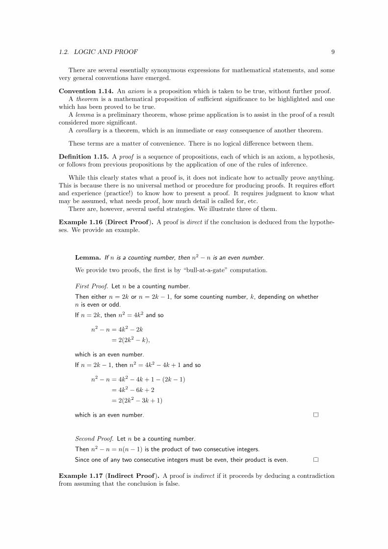
Lemma. If n is a counting number, then n2 − n is an even number.
We provide two proofs, the first is by “bull-at-a-gate” computation.
First Proof. Let n be a counting number.
Then either n = 2k or n = 2k − 1, for some counting number, k, depending on whethern is even or odd.
If n = 2k, then n2 = 4k2 and so
n2 − n = 4k2 − 2k
= 2(2k2 − k),
which is an even number.
If n = 2k − 1, then n2 = 4k2 − 4k + 1 and so
n2 − n = 4k2 − 4k + 1− (2k − 1)
= 4k2 − 6k + 2
= 2(2k2 − 3k + 1)
which is an even number.
Second Proof. Let n be a counting number.
Then n2 − n = n(n− 1) is the product of two consecutive integers.
Since one of any two consecutive integers must be even, their product is even.
Example 1.17 (Indirect Proof). A proof is indirect if it proceeds by deducing a contradictionfrom assuming that the conclusion is false.
10 CHAPTER 1. NOTATION, LOGIC AND PROOF
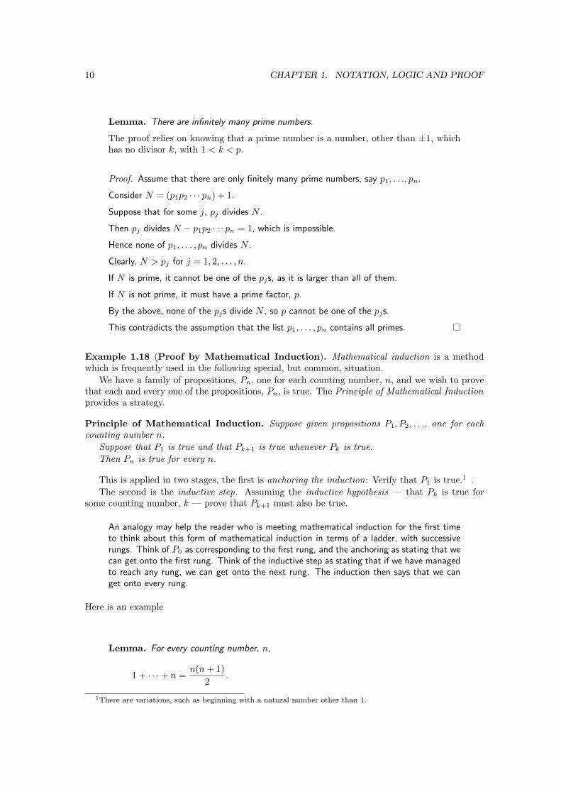
Lemma. There are infinitely many prime numbers.
The proof relies on knowing that a prime number is a number, other than ±1, whichhas no divisor k, with 1 < k < p.
Proof. Assume that there are only finitely many prime numbers, say p1, . . ., pn.
Consider N = (p1p2 · · · pn) + 1.
Suppose that for some j, pj divides N .
Then pj divides N − p1p2 · · · pn = 1, which is impossible.
Hence none of p1, . . . , pn divides N .
Clearly, N > pj for j = 1, 2, . . . , n.
If N is prime, it cannot be one of the pjs, as it is larger than all of them.
If N is not prime, it must have a prime factor, p.
By the above, none of the pjs divide N , so p cannot be one of the pjs.
This contradicts the assumption that the list p1, . . . , pn contains all primes.
Example 1.18 (Proof by Mathematical Induction). Mathematical induction is a methodwhich is frequently used in the following special, but common, situation.
We have a family of propositions, Pn, one for each counting number, n, and we wish to provethat each and every one of the propositions, Pn, is true. The Principle of Mathematical Inductionprovides a strategy.
Principle of Mathematical Induction. Suppose given propositions P1, P2, . . ., one for eachcounting number n.
Suppose that P1 is true and that Pk+1 is true whenever Pk is true.
Then Pn is true for every n.
This is applied in two stages, the first is anchoring the induction: Verify that P1 is true.1 .
The second is the inductive step. Assuming the inductive hypothesis — that Pk is true forsome counting number, k — prove that Pk+1 must also be true.
An analogy may help the reader who is meeting mathematical induction for the first timeto think about this form of mathematical induction in terms of a ladder, with successiverungs. Think of P0 as corresponding to the first rung, and the anchoring as stating that wecan get onto the first rung. Think of the inductive step as stating that if we have managedto reach any rung, we can get onto the next rung. The induction then says that we canget onto every rung.
Here is an example
Lemma. For every counting number, n,
1 + · · ·+ n =n(n+ 1)
2.
1There are variations, such as beginning with a natural number other than 1.
1.3. LOGICAL NOTATION 11
Proof. Take n = 1. Then
1 + · · ·+ n = 1 as there is only one summand, 1.
and
n(n+ 1)
2=
1(1 + 1)
2=
2
2= 1,
showing that P1 is true.
Make the inductive hypothesis that for the counting number, k, Pk is true, that is,
1 + · · ·+ k =k(k + 1)
2
Then
1 + · · ·+ (k + 1) = (1 + 3 + · · ·+ k) + (k + 1)
=k(k + 1)
2+ (k + 1) by the inductive hypothesis
=(k + 1)
2(k + 2) taking out the factor
k + 1
2
=(k + 1)
((k + 1) + 1
)2
,
showing that Pk+1 is true whenever Pk is true.
Hence, by the Principle of Mathematical Induction, if n is any counting number,
1 + · · ·+ n =n(n+ 1)
2.
The above example provides the opportunity and motivation to introduce sigma notation.Notice that in 1+· · ·+n the dots hint that the missing terms are of the form j for j = 2, . . . , n−1.
Then these are added together.
Definition 1.19. Let n be a counting number. For each j ∈ 1, . . . , n, let uj be an expressionof a form which can be added. Then
n∑j=1
uj := u1 + · · ·+ un.
In the last lemma, uj = j and so the lemma states that for every counting number, n,
n∑j=1
j =n(n+ 1)
2.
1.3 Logical Notation
We summarise the logical notation we use, whenever convenient.
P =⇒ Q for “if P , then Q”, or “Q whenever P”, or “P only if Q”;P ⇐⇒ Q for “P if and only if Q”, that is to say P and Q are logically equivalent;P :⇐⇒ Q for “P is defined to be equivalent to Q”;
12 CHAPTER 1. NOTATION, LOGIC AND PROOF
¬P for “Not P”P ∨Q for “P or Q”P ∧Q for “P and Q∀ for “For every . . . ”;∃ for “There is at least one . . . ”;∃! for “There is a unique . . . ”, or “There is one and only one . . . ”.A := B for “A is defined to be (equal to/the same as) B.”
1.4 Exercises
1.4.1. (a) Write down the negation and the converse of the propositionIf a positive integer is divisible by 4 and by 6, then it is divisible by 24.
(b) Write down the negation of the propositionsEvery prime number is odd.Some clever people do dumb things.
1.4.2. Let a be a real number. Prove that, if, for every real number, b,
(a+ b)2 = a2 + b2,
then a = 0.
1.4.3. Use induction to prove that for all counting numbers, n,
(a)
n∑j=1
(2j − 1) = 1 + 3 + . . .+ (2n− 1) = n2.
(b)
n∑j=1
j3 = 13 + 23 + . . .+ n3 =(1
2n(n+ 1)
)2.
(c)
n∑j=0
2n−1 = 1 + 2 + 22 + · · ·+ 2n−1 = 2n
1.4.4. Let a be a positive real number. Prove that, for every counting number, n,
(1 + a)n ≥ 1 + na.
1.4.5. Prove that if n is a counting number, then 32n − 1 is divisible by 8.
1.4.6. Let n be a counting number. Use proof by contradiction to show that if 2n − 1 is a primenumber, then n must, itself, be a prime number.
1.4.7. Prove that the integer, n, is odd if and only if n2 is also odd.
Chapter 2
Sets, First Steps in Algebra andFunctions
2.1 Sets
The mathematics we study in this course can be expressed entirely in terms of sets and functionsbetween sets. We therefore begin with a summary of the set-theoretical concepts and definitionsused in the course. We also use the occasion to summarise further notational conventions we usethroughout this course.
A set is almost any reasonable collection of things. We shall not even attempt a more formaldefinition in this course. The things in the collection are called the elements of the set in question.We write
x ∈ A
to denote that x is an element of the set A and
x /∈ A
to denote that x is not an element of the set A. Note that we do not exclude the possibility thatx be a set in its own right, except that x cannot be A:
We explicitly exclude A ∈ A.
Two sets are considered to be the same when they comprise precisely the same elements, inother words, when every element of the first set is also an element of the second and vice versa.Formally,
Definition 2.1. The set, A, is a subset of the set, B, if and only if x ∈ B whenever x ∈ A. Wewrite
A ⊆ B
whenever this is the case. The sets A and B are the same, denoted A = B, whenever they comprisethe same elements, so that A = B if and only if A ⊆ B and B ⊆ A.
A is a proper subset of B if and only if A is a subset of B, but A 6= B. In such a case we write
A ⊂ B.
13
14 CHAPTER 2. SETS, FIRST STEPS IN ALGEBRA AND FUNCTIONS
Using our notational conventions, given two sets A and B,
A = B :⇐⇒(
(x ∈ A)⇔ (x ∈ B)).
When we wish to describe a set, we can do so by listing all of its elements. Thus, if the set Ahas precisely a, b and c as its elements, then we write
A = a, b, c.
Another way of describing a set is by prescribing a number of conditions for membership ofthe set. In this case we write
x | P (x), Q(x), . . .
to denote that the set in question consists of all those x for which P (x), Q(x), . . . all hold. We canalso read this as the set of all x such that P (x), Q(x, etc. hold.
Example 2.2. Let a, b and c be three different objects. The sets a, b, b, b, a, a, a, a, a, a, b, b, a, b, a, b, aand a, b are all the same set.
Definition 2.3. The empty set, ∅, is the set with no elements.
Observation 2.4. The empty set is a subset of every set, that is, if X is any set, then ∅ ⊆ X.It follows that there is only one empty set.
There are several operations on sets.
Definition 2.5. The union of two sets A and B consists of all those objects which are elementsof one, or other (or both) of the sets. It is denoted by A ∪B. Using the notation above,
A ∪B := x | x ∈ A or x ∈ B.
[Here := has been used to signify that the expression on the left hand side is defined to be equalto the expression on the right hand side.]
We can depict this pictorially by
A B
A ∪B
Example 2.6. If A = 1, 2, 3 and B = 2, 4, then
A ∪B = 1, 2, 3, 4
Lemma 2.7. Let A,B,C be sets. Then
(i) A ∪B = B ∪A.
(ii) A,B ⊆ A ∪B.
(iii) If A ⊆ C, then (A ∪B) ⊆ (C ∪B).
(iv) A ∪B = B if and only if A ⊆ B.
2.1. SETS 15
Proof. As each of the claims follows directly from the definitions, we only prove (ii), leaving theothers as an exercise.
(i) Take a ∈ A. Then a ∈ A or a ∈ B, so that
a ∈ x | x ∈ A or x ∈ B =: A ∪B.
Thus, a ∈ A ∪B whenever a ∈ A, whence
A ⊆ A ∪B
The same argument can be used mutatis mutandis to show that B ⊆ A ∪B.
Definition 2.8. The intersection of the sets A and B consists of all those objects which areelements of both and is denoted by A ∩B, so that,
A ∩B := x | x ∈ A and x ∈ B.
We can depict this pictorially by
A B
A ∩B
Example 2.9. If A = 1, 2, 3 and B = 2, 4, then
A ∩B = 2.
Lemma 2.10. Let A,B,C be sets. Then
(i) A ∩B = B ∩A.
(ii) A ∩B ⊆ A,B.
(iii) If A ⊆ C, then A ∩B ⊆ C ∩B.
(iv) A ∩B = A if and only if A ⊆ B.
(v) A ∩B ⊆ A ∪B.
Proof. As each f the claims follows readily from the definitions, we prove only (v), leaving the restas an exercise.
A ∩B : = x | x ∈ A and x ∈ B= x | x ∈ B and x ∈ A=: B ∩A
Definition 2.11. Those elements of A that are not also elements of B form a set in their ownright, the relative complement of B in A, which we denote by A \B, so that
A \B := x ∈ A | x /∈ B.
We can depict this pictorially by
16 CHAPTER 2. SETS, FIRST STEPS IN ALGEBRA AND FUNCTIONS
A B
A \B
Example 2.12. If A = 1, 2, 3 and B = 2, 4, then
A \B = 1, 3.
Lemma 2.13. Let A,B,C be sets. Then
(i) A \B = B \A if and only if A ∩B = ∅.
(ii) A \B ⊆ A.
(iii) (A \B) ∩B = ∅.
(iv) If A ⊆ C, then
(a) (A \B) ⊆ (C \B)
(b) (B \ C) ⊆ (B \A)
Proof. (i) If x ∈ A \B, then x must be an element of A without being an element of B.But to be an element of B \A, x must be an element of B, without being an element of A.Plainly, no x can satisfy these two conditions simultaneously.The rest is left as an exercise.
Convention 2.14. When all sets, A,B, . . ., under consideration are subsets of a single fixed set,X, it is customary to call X the universal set, and to indicate this in diagrams by enclosing therepresentations of the sets A,B in a rectangle representing X.
A B
Such diagrams are called Venn diagrams.In such a situation, for A ⊆ X, X \A is referred to as the complement of A, and often written
as A′, or A or CA.
A
A′ = X \A
2.1. SETS 17
Definition 2.15. The (Cartesian) product of the sets A and B consists of all ordered pairs ofobjects, the first of each being an element of A, and the second an element of B. It is writtenA×B, so that,
Lemma 2.17. Let A,B,C be sets, with A,B 6= ∅. Then
(i) A×B = B ×A if and only is A = B.
(ii) If A ⊆ C, then A×B ⊆ C ×B.
Proof. (i) If A = B, then A×B = A×A = B ×A.Conversely, suppose that A×B = B ×A.Take a ∈ A and b ∈ B. Then, by definition, (a, b) ∈ A×B.Since A×B = B ×A, we must have (a, b) ∈ B ×A.By defintion, we must then have a ∈ B and b ∈ A.From the former, it follows that a ∈ B whenever a ∈ A, so that A ⊆ B.From the latter, it follows that b ∈ A whenever b ∈ B, so that B ⊆ A.Since A ⊆ B and B ⊆ A, we must have A = B.The rest is left as an exercise.
We cannot represent the Cartesian product of two sets with Venn diagrams. We can representthe Cartesian product “two dimensionally”, with A as the “horizontal axis” and B as the “verticalaxis”.
B
A
A×B
The reader should be familiar with this in the special case where A = B = R, the set of allreal numbers, which is then referred to as the Catersian plane or co-ordinate plane.
We write ∅ for the empty set, which is the (unique!) set with no elements. Note that it is asubset of every set, that is, if X is any set, then ∅ ⊆ X.
Remark 2.18. It is common to at first confuse ∈ and ⊆, partly because it is common to say x isin X, when we mean that x is a element of the set X (x ∈ X), as well as to say A is in X, whenwe mean that the set A is a subset of the set X.
Be careful to avoid this mistake. Remember the relationship between ∈ and ⊆:
x ∈ X if and only if x ⊆ X.
Relations on sets play a central role in mathematics. Of particular importance for this courseis ordering.
Orderings. We begin mathematics by learning to count, and learn that the counting numberscome in a particular order. Order relations generalise this.
18 CHAPTER 2. SETS, FIRST STEPS IN ALGEBRA AND FUNCTIONS
Definition 2.19. Let be a binary relation on the set X — that is, a relation between pairsof elements of X — and write a b whenever a is related to b in the sense of . Then is anpartial order on X if and only if for all a, b, c ∈ X
(i) a a Reflexivity(ii) If a b and b a, then a = b. Antisymmetry
(iii) If a b and b c, then a c. Transitivity
It is common to write b a for a b.It is customary to write a ≺ b (or b a) to denote that a b, but a 6= b.
The partial ordering on X is a total order on X if and only if, in addition,
(iv) Either a b or b a.
Hence, for elements, a, b of a totally ordered set precisely one of the following holds.
a ≺ b, a = b, a b.
Example 2.20. The number systems familiar from school are totally ordered sets, with beingthe familiar ordering less than or equal to, so that a b if and only if a ≤ b.
Example 2.21. An example of a partially ordered set, which is not totally ordered, is obtainedby taking as X the set of all subsets of a fixed set, Y , which has at least two elements, so that
A ∈ X if and only if A ⊆ Y,
and defining by
A B if and only if A ⊆ B.
We verify that this defines a partial order, but not a total order, on X.Let A,B,C be subsets of Y .
(i) Since every element of A is an element of A, A ⊆ A, or, equivalently, A A.
(ii) Suppose that A B and B A. Then A ⊆ B and B ⊆ A. By Definition 2.1, this isequivalent to A = B.
(iii) Suppose that A B and B C, so that A ⊆ B and B ⊆ C. To show that A C, we mustshow that A ⊆ C. To do this, take any y ∈ A.
Since A ⊆ B, we must have y ∈ B, Then, since B ⊆ C, we must have y ∈ C.
Since we have shown that any element of A is an element of C, we have proved that A ⊆ C,as required.
(iv) Finally, to see that our is not a total order, take two distinct elements, of Y , a 6= b.
Then a /∈ b, whence a 6⊆ b, that is, a 6 b.Similarly b /∈ a, whence b 6⊆ a, that is, b 6 a.
Certain subsets of ordered sets play a prominent part in mathematics.
Definition 2.22. Let X be (partially) ordered by . Take a, b ∈ X. Then x lies between a andb if and only if either a x b or b x a.
The subset I of X is an interval if and only if given a, b ∈ I every element of X which liesbetween a and b is itself an element of I.
Given a, b ∈ X with a ≺ b,
(i) ]a, b[ := x ∈ X | a ≺ x ≺ b is the open interval from a to b,
2.2. ARITHMETIC AND FIRST STEPS IN ALGEBRA 19
(ii) [a, b[ := x ∈ X | a x ≺ b is the interval from a to b, closed at a and open at b.
(iii) ]a, b] := x ∈ X | a ≺ x b is the interval from a to b, open at a and closed at b.
(iv) [a, b] := x ∈ X | a x b is the closed interval from a to b.
It follows directly from their definition that these are all intervals.
Remark 2.23. We use of brackets to denote interval, with the brackets pointing in or out,depending as whether the endpoint in question is included in or excluded from the interval.
Some authors use parentheses where we use brackets pointing outwards, writing, for example,(a, b] where we write ]a, b].
Our notation has the advantage that it unambiguously distinguishes the open interval (a, b) —written ]a, b[ in our notation — from the ordered pair (a, b). The former is a subset of X, whereasthe latter is an element of X ×X.
A number of sets occur with such frequency that special notation has been introduced forthem. These include the sets N, Z, Q, R and C consisting respectively of all natural numbers,all integers, all rational numbers, all real numbers and all complex numbers, which we introducebelow. Explicitly,
We also write N∗ for N \ 0 = 1, 2, 3, . . ., the set of counting numbers.Observe that
N∗ ⊂ N ⊂ Z ⊂ Q ⊂ R ⊂ C.
2.2 Arithmetic and First Steps in Algebra
The above sets, with the exception of the set of complex numbers, are familiar from school. Afeature they share, also familiar from school, is that they allow arithmetic: we can add and multiplythem. We briefly outline the path followed at school, leading from the counting numbers to thereal numbers.
Both addition and multiplication were originally defined for counting numbers.These satisfy several Laws of Arithmetic.Given counting numbers, x, y, z
A1 (x+ y) + z = x+ (y + z) Associativity of an Addition
A4 x+ y = y + x Commutativity of Addition
M1 (x× y)× z = x× (y × z) Associativity of Multiplication
M2 1× x = x = x× 1 Existence of a Multiplicative Neutral Element
M4 x× y = y × x Commutativity of Multiplication
D x× (y + z) = (x× y) + (x× z) and (x+ y)× z = (x× z) + (y × z)Distributivity of Multiplication over Addition
20 CHAPTER 2. SETS, FIRST STEPS IN ALGEBRA AND FUNCTIONS
We extend the counting numbers to the natural numbers by adjoining 0 in a manner whichallows us to extend addition and multiplication. This introduces a new Law of Arithmetic.
Let x be a natural number.
A2 x+ 0 = x = 0 + x Existence of an Additive Neutral Element
This expanded number system has many uses, but also has some limitations. For example, ifwe are given natural numbers, a, b, how do we find natural numbers x, y so that
a+ x = b (♦)
a× y = b (♦♦)
To enable us to solve all equations of the form (♦), we extend the natural numbers to theintegers by adjoining negative numbers in a manner which allows us to extend addition andmultiplication. This introduces a new Law of Arithmetic.
Let x be an integer.
A3 (−x) + x = 0 = x+ (−x) Existence of Additive Inverses
It also enables us to define subtraction by
a− b := a+ (−b)
It cannot be possible to solve all equations of the form (♦♦), because 0× x is always 0, whichmeans that (♦♦) cannot have a solution when a = 0 and b 6= 0.
Fortunately, this is the only exceptional case, and we extend the integers to the rational numbersby adjoining fractions — expressions of the form m
n with m an integer and m a counting number— in a manner which allows us to extend addition and multiplication. This introduces anothernew Law of Arithmetic.
Let x be an rational number.
M3 ( 1x )× x = 1 = x× ( 1
x ) for x 6= 0 Existence of Multiplicative Inverses
This enables us to define division by non-zero rational numbers by
b÷ a := b× 1
afor a 6= 0.
Convention 2.24. We adopt the convention of writing xy instead of x × y when there is nodanger of confusion, as well as the usual conventions on omitting parentheses, so that we writexy + z for (x× y) + z.
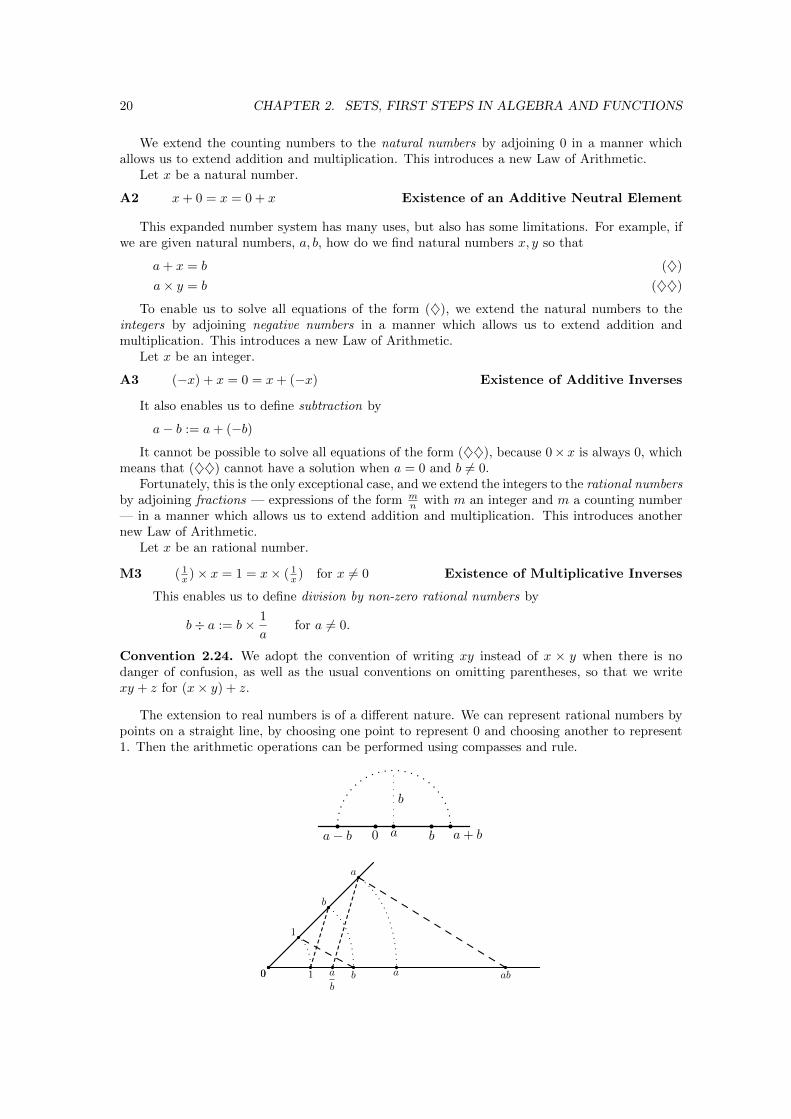
The extension to real numbers is of a different nature. We can represent rational numbers bypoints on a straight line, by choosing one point to represent 0 and choosing another to represent1. Then the arithmetic operations can be performed using compasses and rule.
a b a+ ba− b 0
b
1
1
0 a
a
0 b
b
aba
b
2.2. ARITHMETIC AND FIRST STEPS IN ALGEBRA 21
Moreover, we can construct points on our line which do not represent any rational number.For example, we can construct a point representing the number
√2 by constructing a unit square,
and taking its diagonal.
0 1√
2
Lemma 2.25.√
2 is not rational.
Proof. Suppose that√
2 is rational.Since
√2 is positive, there are counting numbers, m,n with no common factors, such that
√2 =
m
n.
Squaring and multiplying through by n2 yields
m2 = 2n2
from which we see that m2 must be even. But then m must be even, so that m = 2k, for somecounting number, k. Thus
4k2 = 2n2,
or, equivalently,
n2 = 2k2,
whence we get (as above) that n must also be even, say n = 2`, for some counting number, `.Thus both m and n are divisible by 2, contradicting the choice of m and n.
The above discussion indicates, that if we regard the rational numbers as points on a line,with the arithmetic operations performed geometrically, then we may regard the passage from therational numbers to the real numbers as “filling the gaps” between rational numbers. Moreover,it is then obvious that we can extend the arithmetic operations from the rational numbers to allreal numbers.
The study of the set of real numbers and functions defined on it forms our main concern inthis course. We gather together here the main properties and features of the set of real numbers.
The set of real numbers, R, has two distinct structures, the first is the algebraic structurearising from arithmetic, and the second arising from the total ordering (cf Example 2.20). These,and their interplay, are characterised by the following axioms.
Algebraic Axioms
Take x, y, z ∈ R.
A1 x+ (y + z) = (x+ y) + z Associativity of Addition
A2 x+ 0 = x = 0 + x Existence of an Additive Neutral Element
A3 (−x) + x = 0 = x+ (−x) Existence of Additive Inverses
22 CHAPTER 2. SETS, FIRST STEPS IN ALGEBRA AND FUNCTIONS
A4 y + x = x+ y Commutativity of Addition
M1 x(yz) = (xy)z Associativity of Multiplication
M2 x1 = x = 1x Existence of a Multiplicative Neutral Element
M3 ( 1x )x = 1 = x( 1
x ) for x 6= 0 Existence of Multiplicative Inverses
M4 yx = xy Commutativity of Multiplication
D x(y + z) = xy + xz and (x+ y)z = xz + yzDistributivity of Multiplication over Addition
Order Axioms
Take x, y, z ∈ R.
O1 If x < y, then x+ z < y + z.
O2 If x < y and z > 0, then xz < yz.
O3 If x > 0, there is a q ∈ Z, with qx ≤ y < (q + 1)x. Archimidean Property
The properties familiar from school mathematics can be deduced from the above axioms. Wepresent the proofs in some detail so that the reader can see how to construct algebraic proofsfrom axioms, and to demonstrate that the axioms capture the essence of arithemetic: manycommon “facts” about arithmetic are elementary consequences of the axioms. We thus providean exlanation of why these “facts” are true.
Theorem 2.26. Take x, y, z ∈ R.
(i) There is only one additive neutral element, and there is only one multiplicative neutralelement.
(ii) x has precisely one additive inverse, and, if x 6= 0, it has precisely one multiplicative inverse.
(iii) (−(−x)) = x and, if x 6= 0,1(1x
) = x.
(iv) 0x = 0.
(v) (−x) = (−1)x.
(vi) (−x)y = (−(xy)).
(vii) If xy = 0, then either x = 0 or y = 0.
(viii) x > y if and only if x− y > 0.
(ix) x > 0 if and only if (−x) < 0.
(x) x2 ≥ 0, with equality if and only if x = 0.
(xi) x > y if and only if (−x) < (−y)
(xii) x > 0 if and only if 1x > 0.
(xiii) If 0 < x < y, then 0 < 1y <
1x .
2.2. ARITHMETIC AND FIRST STEPS IN ALGEBRA 23
Observation 2.27. These statements follow by direct application of the axioms.Similar proofs apply to similar algebraic settings we meet later, so it is important that the
reader realise that many common properties of real numbers depend only on the algebraic structureand are,therefore, not exclusive to the real numbers: they are shared by any other set with a similaralgebraic structure.
We shall see that the sets of functions of interest to us share many of the structural featuresand algebraic properties of the real numbers, and we shall exploit these when we perform ourcalculations.
Since the reader may not yet be comfortable with rigorous proofs from axioms, we present theproofs, leaving some parts as exercises, which the reader is urged to complete, in order to learn tomaster techniques of proof.
The proofs are not light reading or entertaining. The reader should read, but not dwell on,them, returning to them as needed.
Proof. We turn to proving the theorem.
(i) Take a ∈ R with the property that a+ x = x for every x ∈ R. Then
a = a+ 0 by A2
= 0 by the choice of a
The corresponding statement about the multiplicative neutral element is left to the reader.
(ii) Given x ∈ R, take y ∈ R with y + x = 0. Then
y = y + 0 by A2
= y + (x+ (−x)) by A3
= (y + x) + (−x) by A1
= 0 + (−x) by the choice of y
= (−x) byA2
The corresponding statement about multiplicative inverses is left to the reader.
(iii) This follows from (ii), since, by A3, both (−(−x)) and x are additive inverses of (−x).
The corresponding statement for the multiplicative cased is left to the reader.
(iv) Take x ∈ R. Then
0x = 0x+ 0 by A2
= 0x+ (0x+ (−(0x)) by A3
= (0x+ 0x) + (−(0x)) by A1
= ((0 + 0)x) + (−(0x)) by D
= (0x) + (−(0x)) by A2
= 0 by A3
(v) Take x ∈ R. Then
(−1)x+ x = (−1)x+ 1x by M2
= ((−1) + 1)x by D
= 0x by A3
= 0 by (iv)
Since both (−1)x and (−x) are additive inverses of x, by (ii), (−1)x = (−x).
24 CHAPTER 2. SETS, FIRST STEPS IN ALGEBRA AND FUNCTIONS
(vi) Take x, y ∈ R. Then
(−x)y + xy = ((−x) + x)y by D
= 0y by A3
= 0 by (iv)
Since both (−x)y and (−(xy)) are additive inverses of xy, by (ii), (−x)y = (−(xy)).
(vii) Take x, y ∈ R, with xy = 0 and x 6= 0. Then
y = 1y by M2
= (( 1x )x)y by M3, as x 6= 0
= ( 1x )(xy) by M1
= ( 1x )0 as xy = 0
= 0 by M4 and (iv)
(viii) Take x, y ∈ R.
(a) Suppose that x > y. Then
x− y = x+ (−y) by the definition of subtraction
> y + (−y) by O1
= 0 by A3
Thus x > y only if x− y > 0.
(b) Suppose that x− y > 0. Then
x = x+ 0 by A2
= x+ ((−y) + y) by A3
= (x+ (−y)) + y by A1
= (x− y) + y by the definition of subtraction
> 0 + y by 01 as x− y > 0
= y by A2
(ix) Take x ∈ R. Suppose that x > 0. Then
0 = x+ (−x) by A3
> 0 + (−x) by O1 as x > 0
= (−x) by A2
Thus x > 0 only if (−x) < 0.
The converse is left to the reader.
(x) Take x ∈ R.
If x > 0, then,
x2 = xx
> x0 by 02
= 0 by M4 and (iv)
2.2. ARITHMETIC AND FIRST STEPS IN ALGEBRA 25
If x < 0, then
x2 = xx
= (−(−x))(−(−x)) by (iii)
= ((−1)(−x))((−1)(−x) by (v)
= ((−1)(−1))((−x)(−x)) by M1 and M4
= ((−(−1))((−x)(−x)) by (v)
= 1((−x)(−x)) by (iii)
= (−x)(−x) by M2
> 0 as, by (ix), (−x) > 0
(xi) By (ix), x > y if and only if x+ (−y) = x− y > 0. But then
(−y) = 0 + (−y) by A2
= ((−x) + x) + (−y) by A3
= (−x) + (x+ (−y)) by A1
> (−x) + 0 by O1, as x+ (−y) > 0
= (−x) by A2
The converse is left to the reader.
(xii) Suppose that x > 0.
Then, by (vii), 1x 6= 0, for otherwise ( 1
x )x = 0 6= 1, contradicting M3.
Hence, by (x), ( 1x )2 > 0, and so
1x = 1( 1
x ) by M2
=(x( 1
x ))
(1
x) by M3
= x(1x
)2by M1
> 0(1x
)2by O2, since ( 1
x )2 > 0
= 0 by (iv)
(xiii) Suppose that y > x > 0.
Then 0 < 1x ,
1y , by (xii). Moreover,
x( 1x ) < y( 1
x ) by 02, as 1x > 0,
whence
(x( 1x ))( 1
y ) < (y( 1x ))( 1
y ) by 02, as 1y > 0.
Using M3 and M4, we deduce that
1( 1y ) < (( 1
x )y)( 1y ).
By M2 and M1 we see that
1y < ( 1
x )(y( 1y )).
Using M3 and M2, we deduce that
1y <
1x .
26 CHAPTER 2. SETS, FIRST STEPS IN ALGEBRA AND FUNCTIONS
We presented the above proof in great detail for the benefit of those readers unaccustomedto rigorous proofs. While our proofs will remain rigorous throughout, we shall leave some purelyroutine details to the reader.
Observation 2.28. If we replaced R, the set of all real numbers, by Q, the set of all rationalnumbers, Theorem 2.26 would still be true, and the same proofs would apply. So while we havecaptured axiomatically crucial features of the real numbers, we have not distinguished it fromother sets with similar structure, such as the set of rational numbers. We turn to this next.
Definition 2.29. Let A be a subset of the ordered set X.K is a lower bound for A if and only if K x whenever x ∈ A. A is bounded below if and only
if it has a lower bound.L is an upper bound for A if and only if x L whenever x ∈ A. A is bounded above if and
only if it has an upper bound.A is bounded if it is both bounded below and bounded above.
i ∈ X is the infimum, or greatest lower bound, of S if and only if
(i) i x for all x ∈ A
(ii) If t ∈ X satisfies t x for all x ∈ A, then t i.
In such a case we write inf A = i.If, in addition, inf A = i ∈ A, then i is the minimum of A and we write minA = i.
s ∈ X is the supremum, or least upper bound of S if and only if
(i) x s for all x ∈ A
(ii) If t ∈ X satisfies x t for all x ∈ A, then s t.
In such a case we write supA = s.If, in addition, supA = s ∈ A, then s is the maximum of A and we write maxA = s.
Remark 2.30. If we think of an ordering as a way of indicting the relative “size” of elementsof s set, so that a b signifies that a is “less than or equal to”, or “no greater than”, b, or b is“greater than or equal to”, or “no less than” a, then the supremum is an upper bound with theproperty that no other upper bound can be smaller — hence the expression “least upper bound”.Similarly, the infimum is a lower bound with the property than no greater element can be a lowerbound — hence the expression “greatest lower bound”.
Example 2.31. We take R with its standard total order.
(i) A = x ∈ R | x <√
2 is bounded above, but not below. It has a supremum, namely,√
2,but not a maximum.
(ii) A = x ∈ R | x ∈ Q and x2 ≤ 2 is bounded above and below. It has −√
2 as infimum and√2 as supremum. It has neither a minimum nor a maximum.
(iii) A = x ∈ R | x2 ≤ 2 is bounded above and below. It has −√
2 as minimum and√
2 asmaximum.
Example 2.32. We take Q with its standard total order.
(i) A = x ∈ Q | x <√
2 is bounded above, but not below. It has no supremum. To see this,note that, by Example 2.31, the only possible supremum is
√2. But
√2 is not rational.
(ii) A = (−1)nn
n+1 | n ∈ N∗ = − 12 ,
23 ,−
34 , . . . is bounded above and below. It has −1 as
infimum and 1 as supremum. It has neither a minimum nor a maximum.
We can now formulate the Completeness Axiom, which distinguishes the real numbers. Ourversion is not the usual one, but is equivalent to it.
2.3. THE COMPLEX NUMBERS 27
Completeness Axiom
Every non-empty subset of R which is bounded above, has a supremum.
The axioms we have listed — the Algebraic Axioms, the Order Axioms and the CompletenessAxiom — determine R uniquely. The proof of this deep result is beyond this course.
We went to great trouble to prove several properties of the real numbers, that followed withoutfurther ado from the axioms A1–4, M1–4 and D. We did this because we did not need to useanything about the real numbers except that they satisfy the axioms. As a consequence, theresults apply equally to any system satisfying the same axioms.
Definition 2.33. Any set, F , for which we can define two binary operations, α (“addition”) andµ (“multiplication”) satisfying Axioms A1–4, M1–4 and D axioms is a field .
Example 2.34. The set of all rational numbers, Q, with the usual addition as α and the usualmultiplication as µ, forms a field.
The set of all real numbers, R, with the usual addition as α and the usual multiplication as µ,forms a field.
Neither the set of all natural numbers, N, nor the set of all integers, Z, forms a field with theusual addition as α and the usual multiplication as µ.
One of the most important fields is the field of complex numbers, which we introduce next. Itsimportance is not immediately apparent, but it is crucial to much of mathematics, and indispens-able for applications to theoretical physics, electronics, signal processing, statistics.
2.3 The Complex Numbers
By Theorem 2.26(x), there is no real number, x, satisfying x2 = −1. Yet there is a need for such anumber in many situations. This was recognised in the 15th century. Such a number was termedimaginary. We now introduce and extension of the real number system which includes a squareroot of −1, denoted i, on which we define an “addition” and a “multiplication”. We show thatthis new system is a field, that we can regard the real numbers as elements of this field, and thatwhen we do, the two different additions and two different multiplications coincide.
There are several different ways of constructing the complex numbers from the real numbers.The one we have chosen has the virtue of requiring no further theoretical development. Thereader will meet several other, more conceptual and elegant, constructions later in his/her studyof mathematics.
Definition 2.35. The set, C, of all complex numbers consists of all expressions of the form xu iy,with x, y real numbers.
C := xu iy | x, y ∈ R
The complex numbers xu iy and uu iv agree if and only if x = u and y = v.Given complex numbers, xu iy and uu iv, we define their sum and product by
(xu iy) (uu iv) := (x+ u)u i(y + v)
(xu iy) (uu iv) := (xu− yv)u i(xv + yu)
Remark 2.36. We have used the unusual symbols u, and to keep separate the different“additions” and “muliplications” in use: x+ y and xy denote the customary addition and multi-plication of real numbers, u represents the formal addition of the two parts of a complex numbers,and zw and zw denote the addition and multiplication just introduced for complex numbers.
Once the properties of complex numbers have been established, we shall abandon the exoticnotation, trusting the reader to know from the context which arithmetic operation is intended.
28 CHAPTER 2. SETS, FIRST STEPS IN ALGEBRA AND FUNCTIONS
Remark 2.37. A convenient way to remember this is to think of i as if it were a real number, withthe unusual property that i2 = −1. Treating the new additions and multiplication as ordinaryaddition and multiplication, and replacing i2 by −1 leads to the formulæ used in Definition 2.35.
Lemma 2.38. C forms a field with respect to and .
Proof. The proof consists, for the most part, of routine verifications. We present some here,leaving the rest for the reader.
Take au ib, r u is, uu iv ∈ C.
Associativity of Addition((au ib) (r u is)
) (uu iv) =
((a+ r)u i(b+ s)
) (uu iv) by the definition of
=((a+ r) + u
)u i((b+ s) + v
)by the definition of
=(a+ (r + u)
)u i(b+ (s+ v)
)by the associativity of +
= (au ib)((r + u)u i(s+ v)
)by the definition of
= (au ib)((r u is) (uu iv)
)by the definition of
Existence of a Multiplicative Neutral Element Take au ib and xu iy ∈ C.Then (au ib) (xu iy) := (ax− by)u i(ay + bx).Thus, iau ib is be the multiplicatise neutral element if and only if we have, for all xu iy,
ax− by = x
ay + bx = y
An obvious solution is a = 1, b = 0. Since, by Theorem 2.26(i), there cannot be more than onemultiplicative neutral element, it is 1u i0.
Existence of an Additive Neutral Element It follows immediately from the definition of and Theorem 2.26(i) that 0u i0 is the additise neutral element.
Associativity of Multiplication((au ib) (r u is)
) (uu iv)
=((ar − bs)u i(as+ br)
) (uu iv) by the definition of
=((ar − bs)u− (as+ br)v
)u i((ar − bs)v + (as+ br)u
)by the definition of
=(aru− bsu− asv − brv)u i
(arv − bsv + asu+ bru) by the arithmetic properties of R
=(a(ru− sv)− b(rv + su)
)u i(a(rv + su) + b(ru− sv)
)by the arithmetic properties of R
= (au ib)((ru− sv)u i(rv + su)
)by the definition of
= (au ib)((r u is) (uu iv)
)by the definition of
Existence of Multiplicative Inverses A multiplicative inverse of a u ib ∈ C is a complexnumber, xu iy, satisfying
(au ib) (xu iy) = (ax− by)u (bx+ ay) = 1u i0,
which is equivalent to finding x, y ∈ R such that
ax− by = 1 (i)
bx+ ay = 0. (ii)
2.3. THE COMPLEX NUMBERS 29
Multiplying (i) by a, (ii) by b and adding yields
(a2 + b2)x = a (iii)
Subtracting b times (i) from a times (ii) yields
(a2 + b2)y = −b (iv)
If a2 + b2 6= 0, each of (iii) and (iv) has a unique solution, namely,
x =a
a2 + b2
y =−b
a2 + b2.
If, on the other hand, a2 + b2 = 0, we must have a = b = 0. In this case, (i) has no solution.In other words, if auib 6= 0ui0 (the additive neutral element), then it has a multiplicative inverse,given explicitly by
1
au ib=
a
a2 + b2u
−ba2 + b2
.
Remark 2.39. We shall shortly present a simpler, conceptual proof of the existence of multi-plicative inverses, complete with the formula above.
Observation 2.40. Direct substitution verifies that for all real numbers a, u,
(au i0) (uu i0) = (a+ u)u i0
(au i0) (uu i0) = (au)u i0
This means that we may identify R with the subset xu i0 | x ∈ R of C.When we do so,we see that is just an extension of +.Since au ib = (au i0) (0u ib), we may regard u as a special case of .In light of these observations, we shall write + instead of both u and .
A Geometric Representation of Complex Numbers
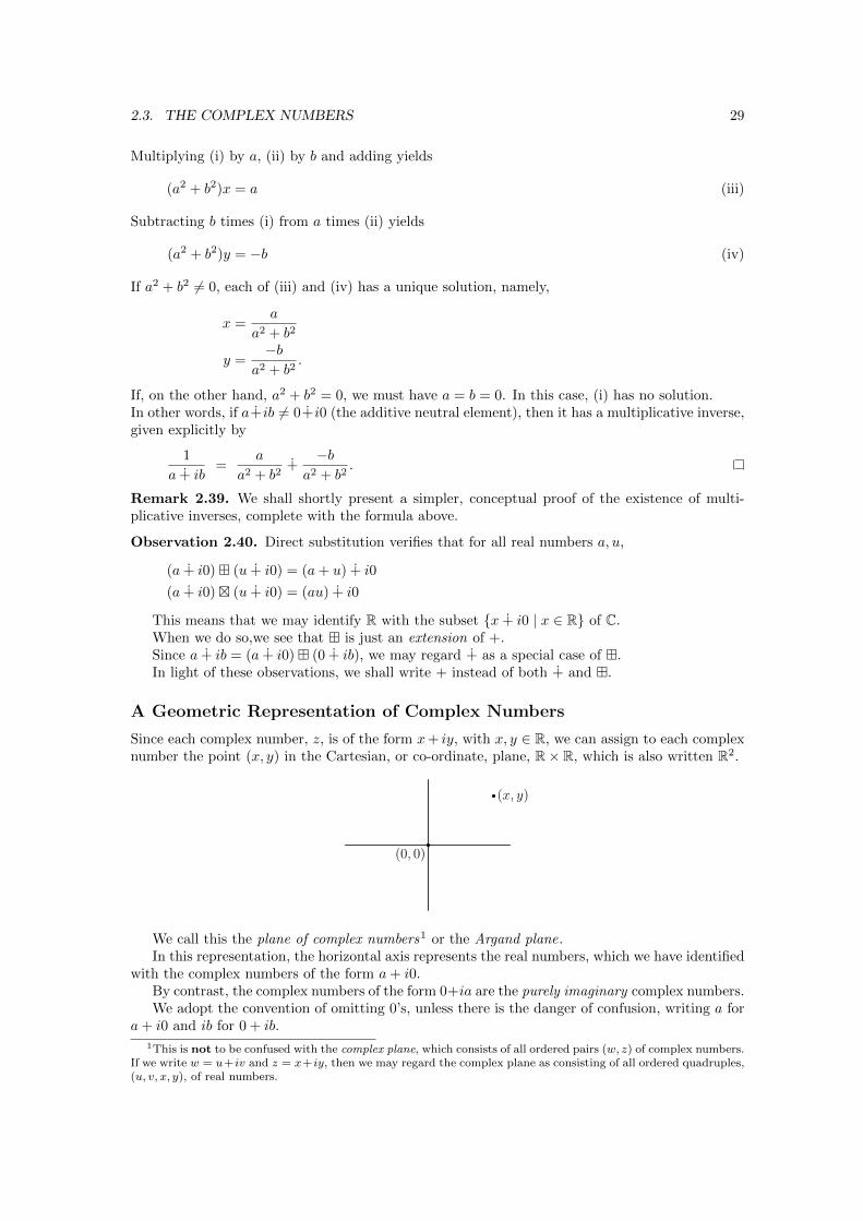
Since each complex number, z, is of the form x+ iy, with x, y ∈ R, we can assign to each complexnumber the point (x, y) in the Cartesian, or co-ordinate, plane, R× R, which is also written R2.
(x, y)
(0, 0)
We call this the plane of complex numbers1 or the Argand plane.In this representation, the horizontal axis represents the real numbers, which we have identified
with the complex numbers of the form a+ i0.By contrast, the complex numbers of the form 0+ia are the purely imaginary complex numbers.We adopt the convention of omitting 0’s, unless there is the danger of confusion, writing a for
a+ i0 and ib for 0 + ib.
1This is not to be confused with the complex plane, which consists of all ordered pairs (w, z) of complex numbers.If we write w = u+iv and z = x+iy, then we may regard the complex plane as consisting of all ordered quadruples,(u, v, x, y), of real numbers.
30 CHAPTER 2. SETS, FIRST STEPS IN ALGEBRA AND FUNCTIONS
Definition 2.41. If z = x+ iy, then x is the real part and y is the imaginary part of z. We write
<(x+ iy) = x and =(x+ iy) = y
The complex conjugate of z = x+ iy is the complex number z := x− iy.
Lemma 2.42. For any complex number z,
(i) <(z) =z + x
2
(ii) =(z) =z − z
2i
(iii) z = z
Proof. Take z = x+ iy ∈ C. Then <(z) = x,=(z) = y and z = x− iy, whence
z = <(z) + i=(z)
z = <(z)− i=(z)
Thus
z + z = 2<(z) that is <(z) =z + x
2
z − z = 2i=(z) that is =(z) =z − z
2i
Finally
z = x− iy = x− (−iy) = x+ iy = z
The use of a co-ordinate plane to represent complex numbers suggests using polar co-ordinates.
(x, y)
(0, 0)
θ
r
(x, 0)
Each point (x, y) in the xy–plane, we can write x = r cos θ and y = r sin θ, for some r ≥ 0 and0 ≤ θ < 2π, with r and θ uniquely determined whenever (x, y) 6= (0, 0) (that is r > 0). Indeed,
r =√x2 + y2 .
Definition 2.43. If z = r cos θ + ir sin θ, then r is the modulus and θ the argument of z. Wewrite
|z| = r and arg(z) = θ
Lemma 2.44. z z = |z|2.
Proof. Let z = x+ iy, with x, y ∈ R. Then, since i2 = −1,
z z = (x+ iy)(x− iy) = x2 − i2y2 = x2 + y2.
2.3. THE COMPLEX NUMBERS 31
Corollary 2.45. z = 0 if and only if |z| = 0, and, if z 6= 0, then
1
z=
z
z z=
z
|z|2.
Thus, if z = a+ ib 6= 0 with a, b ∈ R, then
1
z=
a− iba2 + b2
.
Remark 2.46. This is the conceptual determination of the existence of multiplicative inversespromised in Remark 2.39.
Let the complex numbers z, w be r cos θ + ir sin θ and s cosψ + is sinψ respectively. Then
wz = (r cos θ + ir sin θ)(s cosψ + is sinψ)
= rs((cos θ cosψ − sin θ sinψ) + i(cos θ sinψ + sin θ cosψ)
)= rs(cos(θ + ψ) + i sin(θ + ψ)),
which establishes the next lemma.
Lemma 2.47. Given complex numbers, w, z,
|wz| = |w| |z| and arg(wz) = arg(w) + arg(z),
where this sum is taken modulo 2π.
Corollary 2.48 (de Moivre’s Theorem). If z = r(cos θ+i sin θ) and n is any counting number,then
zn = rn(
cos(nθ) + i sin(nθ))
Proof. We prove this by induction on n.
The case n = 1: When n = 1, we have
z1 = z = r(cos θ + i sin θ) = r1(
cos(1.θ) + i sin(1.θ)),
showing that the proposition is true for n = 1.
The case n ≥ 1: We make the inductive hypothesis that
zn = rn(
cos(nθ) + i sin(nθ))
(IH)
Then
zn+1 = zzn
=(r(cos θ + i sin θ)
)(rn(
cos(nθ) + i sin(nθ)))
by (IH)
= rrn(
cos θ cos(nθ)− sin θ sin(nθ))
+ i(
cos θ sin(nθ) + sin θ cos(nθ))
= rn+1(
cos((n+ 1)θ
)+ i sin
((n+ 1)θ
)),
completing the inductive step.
32 CHAPTER 2. SETS, FIRST STEPS IN ALGEBRA AND FUNCTIONS
Corollary 2.49. Let w be a non-zero complex number and n a counting number. Then theequation
zn = w (∗)
has the n distinct solutions
s1n
(cos(α+2πkn
)+ i sin
(α+2πkn
))(k = 0, 1, . . . , n− 1),
where s := |w| and α = arg(w)).
Proof. Express w and z in modulus-argument form as
w = s(cosα+ i sinα) and z = r(cos θ + i sin θ),
respectively, with r, s > 0 and 0 ≤ α, θ < 2π.By de Moivre’s Theorem (Lemma 2.48), zn = rn
(cos(nθ) + i sin(nθ)
)and 0 ≤ nθ < 2nπ
Thus zn = w if and only if
rn = s
cos(nθ) = cosα
sin(nθ) = sinα
with 0 ≤ nθ < 2nπ, whence
r = s1n ( = n
√s)
nθ ≡ α mod 2π.
Since 0 ≤ nθ < 2nπ, we must have
nθ = α+ 2kπ
with 0 ≤ k < n an integer. In other words,
θ ∈ α+ k 2πn | k = 0, 1, . . . , n− 1.
Thus, the equation zn = w has n solutions
s1n
(cos(α+2πkn
)+ i sin
(α+2πkn
))(k = 0, 1, . . . , n− 1),
where s := |w| and α = arg(w)).These are distinct since, for 0 ≤ β, γ < 2π, cos(α+β) = cos(α+γ) and sin(α+β) = sin(α+γ)
if and only if β = γ.
Exponential Notation for Complex Numbers2
There is a useful alternative way of expressing complex numbers. As a proper justification of thisis beyond the scope of these notes, the reader should regard the following as convenient notationalconvention. A partial justification is provided in MATH102, for expressions of the form ex, withx a real number, and a complete justification is provided in the study of functions of a complexvariable, where x may be any complex number.
The heuristic justification is provided by the facts that the derivative, f ′(x), of the function givenby f(x) = ex is ex and that f ′(x) = Kf(x) if and only if f(x) = AeKx. These concepts andfacts will be proved later in your studies.
2This section may be omitted.
2.4. FUNCTIONS 33
Anticipating results later in these notes, the derivative of cosx is − sinx and that of sinx is cosx.So, if we consider cos θ + i sin θ as a function, f(θ) of θ, we get
f ′(θ) = − sin θ + i cos θ = i (cos θ + i sin θ)
from which we get that
f(θ) = Aeiθ.
Putting θ = 0, we obtain
1 = cos 0 + i sin 0 = f(0) = Aei0 = A,
so that
cos θ + i sin θ = eiθ
This allows us to write the complex number z = x+ iy as z = reiθ, where r is the modulus of z,and, if z 6= 0, θ is the argument of z.
Applying the usual rules of exponents we find that(reiθ
)(seiφ
)= rsei(θ+φ) and
(reiθ
)n= rneinθ
which is a convenient, and suggestive, way of expressing Lemma 2.47 and de Moivre’s Teorem(Corollary 2.48).
By our considerations, we see that eiθ = eiφ is and only if θ − φ is an integer multiple of 2π,which provides a heuristic argument for Corollary 2.49.
This “notational trick” yields Euler’s remarkable formula, relating five fundamental numbers:
eiπ + 1 = 0
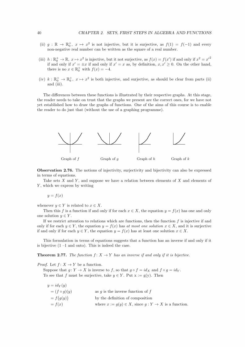
2.4 Functions
To compare sets, we have the notion of a function or map or mapping.
Definition 2.50. A function, map, or mapping consists of three separate data, namely
(i) a domain that is, a set on which the function is defined,
(ii) a codomain, that is, a set in which the function takes its values, and
(iii) the assignment to each element of the domain of definition of a uniquely determined elementfrom the set in which the function takes it values.
This is conveniently depicted diagrammatically by
f : X −→ Y,
or
Xf−−−−→ Y.
Here X is the domain of definition, Y is the set in which the function takes its values and f isthe name of the function. (Note that the function f need not be given in terms of a mathematicalformula.) We write X = dom(f) and Y = codom(f) to indicate that X is the domain and Y thecodomain of f .
Even though both the domain and co-domain are indispensable components of a function, wedo often denote the function f : X → Y by f alone, but only when there is no danger of confusion.
34 CHAPTER 2. SETS, FIRST STEPS IN ALGEBRA AND FUNCTIONS
If we wish to express explicitly that the function, f : X → Y, assigns the element y ∈ Y to theelement x ∈ X, then we write f : x 7→ y or, equivalently, y = f(x). (This latter form is certainlyfamiliar to the reader.)
Sometimes the two parts are combined as
f : X −→ Y, x 7−→ y
or as
f : X −→ Y
x 7−→ y.
How to Think of Functions
We view functions as providing the means to compare sets, because this is the role they play inour investigations.
It is important for the reader to realise the concept of “function” is at the core of mathematics.
The significance of this concept and the need for an abstract definition become clear once theorigin is understood.
Like other fundamental concepts in mathematics, the notion of ”function” is the expression withas much precision as possible, of insights/intuitions from “every-day life”.
Here is a short list of non-mathematical phenomena that motivate the definition of a function.
1. We say “A is a function of B”, when we mean that B determines A..
2. A car manufacturing plant takes the various components and assembles them into cars.
3. A map of Armidale.
4. Cause and effect: each “cause” determines its “effect”.
Superficially, these seem to have little to do with each other. Yet each illustrates the essentialfeatures of functions.
In each case we begin with something — B, or car components, or Armidale, or causes — and,by some process or other, obtain a definite result — A, or a car, or a picture/diagram on a sheetof paper, or effects.
We can regard this as an “input-output” scheme. The function the processing of the input toproduce the resulting output.
Thus the function takes any suitable input — the set of suitable inputs is the domain of thefunction — and processes them to provide an output — the set of all potential outputs is thecodomain of the function.
In a nutshell, it is useful to think of functions as the mathematical formulation of processes leadingto unambiguous results.
Example 2.51. Let X and Y both be the set of all human beings.
(i) f : X −→ Y, x 7−→ y, where y is the (biological) father of x.
As each human being has one and only one biological father, f assigns to each element ofthe domain, a uniquely determined element of the co-domain. It is therefore a function.
(ii) g : X −→ Y, x 7−→ y, where y is the (biological) son of x.
This fails to be a function for two reasons.
(a) Since not everyone has a son, there are elements of the domain to which g assigns noelement of the co-domain.
2.4. FUNCTIONS 35
(b) Since some people have more than one son, there are elements of the domain to whichg assigns more than one element of the co-domain.
Definition 2.52. The identity function, on the set X, is the function idX
defined by
idX
: X −→ X, x 7−→ x,
that is, idX
(x) = x.
Notice that both the domain and codomain must be precisely X for this definition to specifythe identity function.
Example 2.53. We can express the algebraic operations on numbers in terms of functions. Thefact that to each pair of numbers we assign their (uniquely determined) sum and product meansthat we have two functions
α : R× R −→ R, (x, y) 7−→ x+ y
β : R× R −→ R, (x, y) 7−→ xy
Such functions are binary operations, because they assign to each ordered pair of elements ofa set a uniquely determined element of that set.
Definition 2.54. If f assigns y ∈ Y to x ∈ X, then y is the image of x under f or simply theimage of x.
The functions f and g are equal, written f = g, if and only if
(i) dom(f) = dom(g)
(ii) codom(f) = codom(g)
(iii) f(x) = g(x) for every x ∈ dom(f).
In other words, to be the same, two functions must share both domain and codomain as wellas agreeing everywhere.
Remark 2.55. A function (or map, or mapping) is not just a formula.Example 2.51 shows, not every function can be expressed by a formula.Even when a function is given by a formula, that formula need not be unique.Proving that two different formulæ define the same function can be a significant theorem.For example, Pythagoras’ Theorem states, in effect, that the function
f : R −→ R, x 7−→ 1
is the same function as
g : R −→ R, x 7−→ cos2 x+ sin2 x,
despite their being given by different formulæ.Furthermore, there are distinct functions whose domains agree, which agree at every point
(and therefore have the same range). Thus the only difference between them is that they havedifferent codomains: They only differ in the values they do not take!. (At this stage, it may seempeculiarly pedantic to distinguish such functions, but there are important algebraic and geometricexamples, whose detailed study lies beyond the scope of these notes.)
Finally, functions are sometimes given by different formulæ in different parts of its domain, forexample
f : R −→ R, x 7−→
−x for x < 0
x for x ≥ 0
This is called piecewise definition,.
36 CHAPTER 2. SETS, FIRST STEPS IN ALGEBRA AND FUNCTIONS
Lemma 2.56. Given functions g : A → Y and h : B → Y such that g(x) = h(x) wheneverx ∈ A ∩ B, there is a unique function f : A ∪ B → Y such that f(a) = g(a) for all a ∈ A andf(b) = h(b) for all b ∈ B.
Proof. Put X := A ∪B and define f by
f : X −→ Y, x 7−→
g(x) if x ∈ Ah(x) if x ∈ B
.
This definition is forced by the requirement that f(a) = g(a) for a ∈ A and f(b) = h(b) forb ∈ B. Since it is the only possible definition of f satisfying our requirement, there cannot bemore than one function meeting our requirements.
The only question remaining is whether there is any such function at all, or, equivalently,whether our f is, in fact, a function.
(i) Since X = A ∪B is the union of two sets, it is, itself, a set.
(ii) Y is, by hypothesis, also a set.
(iii) Take x ∈ X. Since X = A ∪B, either x ∈ A or x ∈ B (or possibly both).
If x ∈ A, then f assigns g(x) ∈ Y to x, and g(x) is uniquely determined, since g : A→ Y isa function.
If x ∈ B, then f assigns h(x) ∈ Y to x, and h(x) is uniquely determined, since h : B → Y isa function.
Hence, f : X → Y is a function unless it happens to assign two different elements of Y tosome x ∈ X. This can only occur when x ∈ A ∩ B, for then f assigns both g(x) and h(x)to x. But, by assumption, g(x) = h(x) whenever x ∈ A∩B, so that f : X → Y is, indeed, afunction.3
Observation 2.57. In Lemma 2.56, the fact that X = A ∪B ensures that there cannot be morethan one function meeting our requirements, and the fact that g and h agree on A∩B ensure thatthere is at least one such function.
Example 2.58. Consider the definition
| | : R −→ R, x 7−→
−x if x ≤ 0
x if x ≥ 0.
To see that | | is a function, we define R−0 := x ∈ R | |x ≤ 0 and R+0 := x ∈ R | x ≥ 0.
Then
(i) g : R−0 → R, x 7→ −x and h : R+0 → R, x 7→ x are, plainly, functions;
(ii) R = R−0 ∪ R+0 ;
(iii) R−0 ∩ R+0 = 0 and g(0) = −0 = 0 = h(0).
Hence, by Lemma 2.56, | | : R→ R is a function.
We adhere to the practice of specifying functions in a formally correct manner, stating itsdomain and co-domain rather than just a formula, so that it can become ordinary matter ofcourse for the reader do so as well.
A function f : X −→ Y can be represented by means of its graph.
3We also say that f is well defined.
2.4. FUNCTIONS 37
Definition 2.59. The graph, Gr(f), of the function f : X → Y is
Gr(f) := (x, y) ∈ X × Y | y = f(x).
This representation should be familiar from school.
Definition 2.60. The range or image, im(f), of the function f : X → Y is the subset of Y definedby
im(f) := y ∈ Y | y = f(x) for some x ∈ X.
Note that im(f) ⊆ codom(f), with equality holding only sometimes. For example if f : R −→ Ris defined by f(x) := 1 for every x ∈ R, then im(f) = 1 6= R = codom(f).
Definition 2.61. Given a function f : X → Y and subsets A of X and B of Y , define
f(A) := y ∈ Y | y = f(x) for some x ∈ Af−1(B) := x ∈ X | f(x) ∈ B.
Then f(A) is the image of A under f and f−1(B) is the inverse image of B under f , or thepre-image of Bunder f .
We can characterise subsets purely in terms of functions.
Definition 2.62. Suppose that X ⊆ Y . The inclusion function is
iYX : X −→ Y, x 7−→ x
On the left x is considered as element of X . On the right, it is considered as element of Y .
Lemma 2.63. Let X,Y be sets. Then X ⊆ Y if and only if
X −→ Y, x 7−→ x (∗)
is a function.
Proof. The proof is essentially a restatement of the definition of a function.Suppose that X ⊆ Y . Then, by definition, every element of the set X is also an element of the
set Y . Since every x trivially determines itself uniquely, (∗) meets all three requirements to definea function.
For the converse, suppose that (∗) defines a function, then since each x ∈ X is mapped to itself,but now as element of Y , each element of X must be an element of Y , that is to say, X ⊆ Y .
Definition 2.64. Given a function f : X → Y and a subset A of X we can use f to define afunction f |
A: A→ Y , called the restriction of f to A by means of
f |A
(x) = f(x) for every x ∈ A.
Note that unless of course A = X, this is not the same function as f , even though the twofunctions agree everywhere they are both defined.
Functions can sometimes be composed.
Definition 2.65. Given functions f : X → Y and g : Y → Z their composition, g f , is thefunction defined by
g f : X −→ Z, x 7−→ g(f(x)
),
as long as codom(f) = dom(g) = Y .
38 CHAPTER 2. SETS, FIRST STEPS IN ALGEBRA AND FUNCTIONS
In such a case,
dom(g f) = dom(f)
codom(g f) = codom(g)
im(g f) ⊆ im(g).
The first two statements are true by definition and the last is an immediate consequence.Equality need not hold in the last of these statements. To see this consider the functions
f : R→ R, x 7→ 1 and g : R→ R, y 7→ y. Clearly im(g f) = 1 6= R = im(g).
Example 2.66. The function f : R→ R, x 7→ 2x2+1 can be written as a composition f = jhgwhere g, h, j are the functions
g : R −→ R, x 7−→ x2
h : R −→ R, y 7−→ 2y
j : R −→ R, z 7−→ z + 1
so that
f(x) = j(h(g(x)
))= j(h(x2)
)= j(2x2) = 2x2 + 1.
Observation 2.67. The composition in Example 2.66 describes, step-by-step, how we actuallyevaluate the function. To this extent, it simply describes what we actually do when we have slightlycomplex calculations, illustrating one of the important practical applications of the compositionof functions: we decompose complicated functions as the composition of simpler ones in order tofacilitate computation.
Even more importantly, we shall use such decomposition of functions for theoretical purposes,which yield techniques and formulæ for calculating limits and derivatives.
It also provides explanations for common constructions, such as the restriction of functions.Given A ⊆ X and a function f : X → A, the restriction f |
A: A→ Y is, in fact, the composition
of f and the inclusion of A into X:
f |A
= f iX
A.
Observation 2.68. Sometimes you will see the composition of functions f and g even whencodom(f) 6= dom(g), as long as im(f) ⊆ dom(g). While this is not strictly correct, we can justifyit within our formal framework.
Take f : X → Y and g : A→ Z, with B := im(f) ⊆ A ∩ Y .We may then replace f by
f : X −→ B, x 7−→ f(x),
and define g f : X → Z to be the composite g iAB f .
The composition of functions is associative.
Lemma 2.69. Take functions h : W → X, g : X → Y and f : Y → Z. Then the compositions(f g) h : W → Z and f (g h) : W → Z are the same function.
Proof. Since dom((f g) h
)= domh = dom(g h) = dom
(f (g h)
)= W .
Since codom((f g) h
)= codom(f g) = codom f = codom
(f (g h)
)= Z.
It only remains to show that for w ∈W ,((f g) h
)(w) =
(f (g h)
)(w). But, for w ∈W ,(
(f g) h)(w) := (f g)
(h(w)
):= f
(g(h(w)
))=: f
((g h)(w)
)=:(f (g h)
)(w)
2.4. FUNCTIONS 39
The identity functions act as neutral elements with respect to composition.
Lemma 2.70. Let f : X → Y be a function, then
idY f = f
f idX = f.
Proof. Take x ∈ X. Then
(idY f)(x) := idY(f(x)
):= f(x)
(f idX)(x) := f(idX(x)
):= f(x)
Sometimes the effect of one function can be “undone” by another, if the first assigns y to x,the second allows us to determine x from y. Composition of functions allows us to formulate thisprecisely.
Definition 2.71. The functions f : X → Y and g : Y → X are inverse functions if and only ifg f = idX and f g = idY .
A function cannot have more than one inverse.
Lemma 2.72. Let e, g : Y → X be functions inverse to f : X → Y . Then e = g.
Proof. Since dom(e) = dom(g) = Y and codom(e) = codom(g) = X , we only need to verify thatfor all y ∈ Y , e(y) = g(y).
Take y ∈ Y . Then
e(y) = (e (idY )(y) by Lemma 2.70
=(e (f g)
)(y) as f g = idY
=((e f) g
)(y) as composition of functions is associative
= (idX g)(y) as e f = idX
= g(y) by Lemma 2.70
Observation 2.73. The fact that a function, f : X → Y , cannot have more than one inversejustifies the notation f−1 usually used to denote the function Y → X inverse to f , for it isuniquely determined by f whenever f is invertible.
Finally, we introduce some important properties of functions.
Definition 2.74. The function f : X −→ Y is said to be
(i) 1–1 or injective or mono if and only if for all x, x′ it follows from f(x) = f(x′) that x = x′;
(ii) onto or surjective or epi if and only if given any y ∈ Y there is an x ∈ X with f(x) = y —in other words im(f) = codom(f);
(iii) 1–1 and onto or bijective or iso if and only if it is both 1–1 and onto.
Thus a function is injective if and only if it distinguishes different elements of its domain:different elements of its domain are mapped to different elements of its codomain.
Similarly, a function is surjective if and only if its range coincides with its codomain.
Example 2.75. We write R+0 for x ∈ R | x ≥ 0 .
(i) f : R→ R, x 7→ x2 is neither injective nor surjective, as f(1) = f(−1) and there is no x ∈ Rwith f(x) = −4.
40 CHAPTER 2. SETS, FIRST STEPS IN ALGEBRA AND FUNCTIONS
(ii) g : R → R+0 , x 7→ x2 is not injective, but it is surjective, as f(1) = f(−1) and every
non-negative real number can be written as the square of a real number.
(iii) h : R+0 → R, x 7→ x2 is injective, but it not surjective, as f(x) = f(x′) if and only if x2 = x′
2
if and only if x′ = ±x if and only if x′ = x as, by definition, x, x′ ≥ 0. On the other hand,there is no x ∈ R+
0 with f(x) = −4.
(iv) k : R+0 → R+
0 , x 7→ x2 is both injective, and surjective, as should be clear from parts (ii)and (iii).
The differences between these functions is illustrated by their respective graphs. At this stage,the reader needs to take on trust that the graphs we present are the correct ones, for we have notyet established how to draw the graphs of functions. One of the aims of this course is to enablethe reader to do just that (without the use of a graphing programme).
Graph of f Graph of g Graph of h Graph of k
Observation 2.76. The notions of injectivity, surjectivity and bijectivity can also be expressedin terms of equations.
Take sets X and Y , and suppose we have a relation between elements of X and elements ofY , which we express by writing
y = f(x)
whenever y ∈ Y is related to x ∈ X.
Then this f is a function if and only if for each x ∈ X, the equation y = f(x) has one and onlyone solution y ∈ Y .
If we restrict attention to relations which are functions, then the function f is injective if andonly if for each y ∈ Y , the equation y = f(x) has at most one solution x ∈ X, and it is surjectiveif and only if for each y ∈ Y , the equation y = f(x) has at least one solution x ∈ X.
This formulation in terms of equations suggests that a function has an inverse if and only if itis bijective (1 –1 and onto). This is indeed the case.
Theorem 2.77. The function f : X → Y has an inverse if and only if it is bijective.
Proof. Let f : X → Y be a function.
Suppose that g : Y → X is inverse to f , so that g f = idX and f g = idY .
To see that f must be surjective, take y ∈ Y . Put x := g(y). Then
y = idY (y)
= (f g)(y) as g is the inverse function of f
= f(g(y)
)by the definition of composition
= f(x) where x := g(y) ∈ X, since g : Y → X is a function.
2.4. FUNCTIONS 41
To see that f must be injective, take x, u ∈ X, with f(x) = f(u). Then
u = idX(u)
= (g f)(u) as g is the inverse function of f
= g(f(u)
)by the definition of composition
= g(f(x)
)as f(u) = f(x)
= (g f)(x) by the definition of composition
= x
For the converse, suppose that f is bijective.Define g : Y → X by g : y 7→ x if and only if f : x 7→ y.It follows immediately that f
(g(y)
)= y for every y ∈ Y and g
(f(x)
)= x for every x ∈ X.
Thus, g is the inverse of f as long is g is, in fact, a function.Since the domain of g is Y and its co-domain is X, and both are sets, it only remains to verify
that g assigns to each y ∈ Y a uniquely determined x ∈ X.But f is bijective. The surjectiveness of f ensures that for each y ∈ Y , there is some x ∈ X
with f : x 7→ y, and the inectiveness shows there cannot be two such elements in X.
We now consider the case where the set, Y , is ordered, by, say, ≤.
Definition 2.78. The function : X → Y is bounded above if and only if there is a K ∈ Y suchthat for all x ∈ X, f(x) ≤ K.
f is bounded below if and only if there is a B ∈ Y such that for all x ∈ X, B ≤ f(x).f is bounded if and only if it is both bounded below and bounded above.
If the set X is also ordered, by say, , we can ask whether the function f : X → Y respectsthe orders.
Definition 2.79. The function f : X → Y is
(i) (monotonically) non-decreasing if and only if for all a, b ∈ X f(a) ≤ f(b) whenever a b,
(ii) (monotonically) increasing if and only if for all a, b ∈ X f(a) < f(b) whenever a ≺ b,
(iii) (monotonically) non-increasing if and only if for all a, b ∈ X f(b) ≤ f(a) whenever a b,
(iv) (monotonically) decreasing if and only if for all a, b ∈ X f(b) < f(a) whenever a ≺ b,
(v) monotonic if and only if it satisfies one of the four previous conditions and strictly monotonicif and only if either (ii) or (iv) holds.
Example 2.80. Take R with its usual ordering.
(i) The function
f : R −→ R, x 7−→
0 if x ≤ 0
x if x > 0
is monotonically non-decreasing, without being increasing.
(ii) The function
f : R −→ R, x 7−→ −x
is monotonically decreasing.
42 CHAPTER 2. SETS, FIRST STEPS IN ALGEBRA AND FUNCTIONS
(iii) The function
f : R −→ R, x 7−→ x2
is not monotonic because f(−1) > f(0) and f(0) < f(1).
Lemma 2.81. Every strictly monotonic function defined on a totally ordered set is injective..
Proof. Suppose that X is totally ordered and that f : X → Y is monotonically increasing.Take a, b ∈ X, a 6= b.Then either a < b or b < a.In the former case, f(a) < f(b) and in the latter f(b) < f(a).Thus, in both cases f(a) 6= f(b).The case when f is decreasing can be handled similarly.
Lemma 2.82. If g : Y → X is the inverse of the monotonic function f : X → Y , then g ismonotonic.
Proof. Let be the ordering on X and ≤ the ordering on Y .We consider the case when f is increasing and leave the case when f is decreasing to the reader.Take y < y′ in Y , and put x := g(y), x′ = g(y′).If x′ x, then, since f is increasing,
y′ = f(x′) ≤ f(x) = y,
contradicting the choice of x, x′.
We often depict functions using diagrams. We say that the diagram
A B
C
f
gg f
commutes when h = g f , in other words, when the composition g f coincides with h. Similarly,the diagram
A B
C D
f
g
f k
commutes when k j = g f , in other words, when the compositions g f and k j coincide.We can express the fact that the composition of functions is associative — that is to say, iff : W → X, g : X → Y and h : Y → Z are functions then (h g) f = h (g h) — by means ofcommutative diagrams, namely by stating that
A B
C D
f
h
g f h g
2.5. EXERCISES 43
commutes, or, equivalently, that
A B
C D
f
g
h
g fh g
commutes.
2.5 Exercises
2.5.1. Let A,B and C be sets. Show that
(i) A ∩B ⊆ A and A ∩B ⊆ B
(ii) If C ⊆ A and C ⊆ B, then C ⊆ A ∩B
(iii) A ⊆ A ∪B and B ⊆ A ∪B
(iv) If A ⊆ C and B ⊆ C, then A ∪B ⊆ C.
(v) A ∪ (B ∩ C) = (A ∪B) ∩ (A ∪ C)
(vi) A ∩ (B ∪ C) = (A ∩B) ∪ (A ∩ C)
(vii) A \ (B ∩ C) = (A \B) ∪ (A \ C)
(viii) A \ (B ∪ C) = (A \B) ∩ (A \ C)
2.5.2. Given any subset Y of the set X, we write Y ′ = X \Y . Use Venn diagrams to demonstratethat, for all subsets A and B of X,
A \B = A ∩B′.
2.5.3. Let A and B be sets. Show that the following are equivalent.
(i) A ⊆ B
(ii) A ∩B = A
(iii) A ∪B = B
2.5.4. Determine which of the following sets
(a) is bounded below,
(b) has an infimum (greatest lower bound),
(c) has a minimum,
(d) is bounded above,
(e) has a supremum (least upper bound),
(f) has a maximum.
(i) x ∈ Z | x ≤√
2
44 CHAPTER 2. SETS, FIRST STEPS IN ALGEBRA AND FUNCTIONS
(ii) x ∈ Q | x ≤√
2
(iii) x ∈ R | x ≤√
2
(iv) x ∈ R | x ≤√
2 and x ∈ Q
(v) x ∈ Z | x2 < 2
(vi) x ∈ Q | x2 < 2
(vii) x ∈ R | x2 < 2
(viii) ]0, 1] := x ∈ R | 0 < x ≤ 1].
Explain your answer.
2.5.5. Let a be a real number. Show that the equation x2 = a has
(i) no real solution if a < 0,
(ii) one real solution if a = 0.
(iii) two real solutions if a > 0.
2.5.6. Let a, b be real numbers. Prove that it a < b < 0, then
1
a>
1
b> 0
2.5.7. Prove that√
3 is not rational.
2.5.8. Let a and b be real numbers. Prove that
maxa, b =a+ b+ |a− b|
2
mina, b =a+ b− |a− b|
2
2.5.9. When we take the rational numbers with their usual ordering, there is no rational number“next” after a given one.
There are ways of arranging the rational numbers in such a order that each is followed bya next one. One way is based on how we represent positive rational numbers as quotients p
q ofcounting numbers, without worrying about when different quotients represent the same rationalnumber.
1
1,
2
1,
1
2,
3
1,
2
2,
1
3,
4
1,
3
2,
2
3,
1
4, · · ·,
Show thatp
qoccupies the
[12 (p+ q − 1)(p+ q − 2) + q
]thplace from the left.
2.5.10. Let a, be real numbers. Show that if a < b+ ε, for every ε > 0, then a ≤ b.
2.5.11. Take counting numbers m,n. This exercise shows that ifm
napproximates
√2 from below,
thenm+ 2n
m+ nis a better approximation, but from above:
Prove that ifm
n<√
2, then
√2 <
m+ 2n
m+ nand
m+ 2n
m+ n−√
2 <√
2− m
n.
2.5. EXERCISES 45
2.5.12. Express each of the following complex numbers in the form x+ yi, with x, y ∈ R.
(i) (2− i)(2 + i)
(ii) (6 + 5i)(2− 7i)
(iii)2− i1 + 2i
(iv)1− 3i
(2 + i)2+
1 + i3
1 + i
Find the modulus and complex conjugate of each.
2.5.13. Show that1 + cos θ + i sin θ
1 + cos θ − i sin θ= cos θ + i sin θ.
2.5.14. Find all complex numbers, z, such that z2 = 6 + 8i.
2.5.15. Extend de Moivre’s Theorem (Corollary 2.48) by showing that if m is an integer and n acounting number, then for every complex number z = r(cos θ + i sin θ)
zn = rmn
(cos(
m
nθ) + i sin(
m
nθ))
2.5.16. Recalling that R−0 = r ∈ R | r ≤ 0 and R+0 = r ∈ R | r ≥ 0, decide which of the
following is a function, explaining your answer.
(a) Let X be the set of all current telephone subscribers in Australia. Let Y be the set of alltelephone numbers in use in Australia.Define f : x −→ Y, x 7−→ y, where y is x’s telephone number.
(b) Let X,Y be R, the set of all real numbers.Define f : X −→ Y, x 7−→ y, where y = x2.
(c) Let X,Y be R, the set of all real numbers.Define f : X −→ Y, x 7−→ y, where x = y2.
(d) Let X,Y be the set of all non-negative real numbers, R+0 := r ∈ R | r ≥ 0.
Define f : X −→ Y, x 7−→ y, where x = y2.
(e) Let X,Y be R, the set of all real numbers.
Define f : X −→ Y, x 7−→ y, where y =
x if x ≤ 0
−x if x ≥ 0
2.5.17. Let f : X → Y be a function, and A ⊆ X a subset of X. Then the image of A under f ,f(A) is the subset of Y defined by
f(A) := f(x) | x ∈ A = y ∈ Y | y = f(x) for some x ∈ X
Show that if A,B ⊆ X, then
(i) f(A ∪B) = f(A) ∪ f(B)
(ii) f(A ∩B) ⊆ f(A) ∩ f(B)
Find an example where f(A ∩B) 6= f(A) ∩ f(B).
46 CHAPTER 2. SETS, FIRST STEPS IN ALGEBRA AND FUNCTIONS
2.5.18. Decide which of the following functions can be composed, and for those which can, whatis their composition? Justify your answer.
f : R −→ R, x 7−→ x2
g : R+0 −→ R, y 7−→ 2y
h : R −→ R, z 7−→ z + 2
k : R −→ R+0 , u 7−→ u2
2.5.19. Take X ⊆ R.When do the following define functions?
f : X −→ R, x 7−→√x2 − 3x+ 2
g : X −→ R, x 7−→ tan(3x+ 2)
Which of these functions is injective (1–1)?
2.5.20. Take functions f : X → Y and g : Y → Z.
(a) Show that if f and g are both surjective (onto), then g f : X → Z is also surjective.
(b) Show that if g f is surjective, then so is g.
(c) Find an example where g f is surjective, but f is not.
2.5.21. Decide whether the following functions are monotonic, explaining your answer carefully.
(a) f : R−0 −→ R, x 7−→ x2
(b) g : R+0 −→ R, x 7−→ x2
(c) h : R −→ R, x 7−→ x2
(d) h : R −→ R, x 7−→ x3
Chapter 3
Real Valued Functions
Few people study or pursue mathematics out of interest in mathematics itself. Most do so becausemathematics is needed for their main interest, most commonly for modelling phenomena, processesor complex systems in the natural sciences, in engineering, in economics and elsewhere.
Mathematical modelling is used where numerically quantifiable observations and data are avail-able. One is typically interested in the relationship between different quantifiiable observables,and is seeking both an explanation for their behaviour and the ability to predict the behaviour.
When controlled, repeatable experiments are not available, we rely on repeated observationsand employ statistical analysis to draw inferences. When controlled, repeatable experiments areavailable, we typically use real valued functions, that is functions of the form f : X → R. In thesimplest cases, we use real valued functions of a real variable, that is to say, when X ⊆ R. Thebulk of this course is devoted to their study: univariate calculus.
The fact that the co-domain of the functions we study is R has significant consequences. Theset of all functions from a fixed set, X, to R, which we denote by F(X), inherits most of theproperties of the real numbers. We can define an addition and a multiplication on F(X), whichallows us to calculate with functions in almost an identical manner with calculations with realnumbers: all but one of the algebraic axioms hold. F(X) also inherits an ordering from R, butthis is not a total ordering.
Remarkably, all of this is true for any set X, as long as it is not empty. This means that wemay regard F(X) as a generalisation of R.
When we specialise to the case X = R, we obtain F(R), which admits an additional operation,the composition of functions. This rich algebraic structure is what makes F(R) so powerful.
We study these explicitly, because this structure simplifies subsequent analysis, applicationsand computations.
We discuss some specific important functions before turning to the general structure.
3.1 Constant Functions
Choose a fixed real number r. For any non-empty set X we have the constant function
fr : X −→ R, x 7−→ r.
Different choices of r correspond to different choices of constant function X → R.
Identifying the real number, r, with the function X → R that only takes the value r, allows usto regard R as a subset of F(X) whenever X is not empty.
47
48 CHAPTER 3. REAL VALUED FUNCTIONS
3.2 The Case of X a Finite Set
3.2.1 X = ∗When X is a singleton — a set with precisely one element — a function f : X → R is the samething as choosing a single real number: the function
f : ∗ −→ R, ∗ 7−→ f(∗)
may be identified with the real number f(∗). In this case, we can identify F(X) with R.
3.2.2 X = 1, 2A function f : 1, 2 → R is completely determined by the pair of real numbers (f(1), f(2)).
If we write x1 for f(1) and x2 for f(2), then we can identify F(X) with
(x1, x2) | x1, x2 ∈ R,
the set of all ordered pairs of real numbers, R× R, which is also denoted R2.
3.2.3 X = 1, . . . , nA function f : 1, . . . , n → R is completely determined by the n-tuple of real numbers (f(1), . . ., f(n)).
If we write xj for f(j) with j ∈ 1, . . . , n, then we can identify F(X) with
(x1, . . . , xn) | x1, . . . , xn ∈ R,
the set of all ordered pairs of real numbers, R× · · · × R, which is also denoted Rn or
n∏j=1
R.
We often write (xj)nj=1 for the n-tuple (x1, . . . , xn).
3.3 The Case of X = NA function f : N → R is the same thing as choosing for each natural number, n. a corre-sponding real number, f(n). Thus f is completely determined by the sequence of real numbersf(0), f(1), . . . , f(n), . . ., which we denote by
(xn)n∈N,
where xn := f(n). We study sequences in detail later.
3.4 The Case of X = R
3.4.1 The Identity Function
The most important function R→ R is the identity function
idR : R −→ R, x 7−→ x
3.4. THE CASE OF X = R 49
3.4.2 The Absolute Value Function
The absolute value or modulus may be thought of geometrically by representing each real numberas a point on a line, in which case the absolute value of a real number is the distance of the pointrepresenting it from the point representing 0. Formally
| | : R −→ R, x 7−→
−x if x < 0
0 if x = 0
x if x > 0
We showed in Example 2.58 that x 7→ |x| does indeed define a function R→ R.We summarise the properties of this function.
Theorem 3.1. Take x, y ∈ R.
(i) |x| ≥ 0 and |x| = 0 if and only if x = 0. Moreover, |x| = max−x, x.
(ii) |xy| = |x| |y|
(iii) |x2| = x2
(iv) −|x| ≤ x ≤ |x|
(v) |x+ y| ≤ |x|+ |y|
(vi)∣∣|x| − |y|∣∣ ≤ |x− y|
Proof. Take x, y ∈ R.
(i) This is immediate from the definition.
(ii) xy < 0 if and only if either x < 0 and y > 0, or x > 0 and y < 0.
Then either |x| = −x and |y| = y, or |x| = x and |y| = −y.
In both cases |x| |y| = −xy = |xy|.
xy = 0 if and only if x = 0 or y = 0, that is, |x| = 0 or |y| = 0.
In both cases |x| |y| = 0 = |xy|.
xy > 0 if and only if either x < 0 and y < 0, or x > 0 and y > 0.
Then either |x| = −x and |y| = −y, or |x| = x and |y| = y.
In both cases |x| |y| = xy = |xy|.
(iii) This follows from the fact that x2 is never negative.
(iv) Note that since |x| ≥ 0, we always have −|x| ≤ |x|.The result follows from the fact that either x = −|x| or x = |x|.(This argument also shows that −|x| ≤ −x ≤ |x|.)
(v) Since |x|, |y|, |x+ y| ≥ 0, it is enough to show that
Definition 3.2. A polynomial with real coefficients in the indeterminate t, or real polynomial isan expression of the form
p(t) = a0 + a1t+ a2t2 + · · ·+ ant
n =
n∑j=0
ajtj
where each aj is a real number and an 6= 0 if n 6= 0.If an 6= 0, then n is the degree of p (or p(t)), and we write
deg p = n.
We write R[t] for the set of all real polynomials in the indeterminate t.
Observation 3.3. It is important to remember that the t in a polynomial is not a real number. Itis an indeterminate. The “addition” and the “multiplication” in the notation are not (arithmetic)addition and multiplication, they are formal operations.
This is often difficult to grasp at first and, at this stage, may seem to be mere sophistry.However the point is an important one.
Lemma 3.4. Each polynomial, p =
n∑j=0
ajtj ∈ R[t], defines a function
fp : R −→ R, x 7−→n∑j=0
ajxj ,
where now the addition and multiplication are the usual arithmetic operations and we adopt theconvention that for every real number, x, x0 = 1.
Proof. The fact that fp is a function follow from the definition and properties of the usual arith-metic operations.
Observation 3.5. We regard the function fp as obtained by evaluating the polynomial p.
Definition 3.6. The function f : R → R is called a polynomial function is there is a polynomialp ∈ R[t] with f = fp.
Example 3.7. The functions
f : R −→ R, x 7−→ 2x2 + 3x − 1
idR : R −→ R, x 7−→ x
are polynomial functions, with f = fp, where p(t) = −1 + 3t+ 2t2, and idR = fq, where q(t) = t.
3.4. THE CASE OF X = R 51
Example 3.8. Even though cos2 t+ sin2 t is not a polynomial, the function
f : R −→ R, x 7−→ cos2 x+ sin2 x
is a polynomial function, as, by Pythagoras’ Theorem, cos2 x+ sin2 x = 1 for every real number x.Hence f = f1, where 1 is the polynomial, a0, of degree zero with a0 = 1.This example illustrates why we distinguish polynomials from polynomial functions.
3.4.4 Trigonometric Functions
The two basic trigonometric functions R→ R are
sin : R −→ R, x 7−→ sinx
cos : R −→ R, x 7−→ cosx
should be familiar from high school. They are not polynomial functions. This fact is not imme-diately obvious, but we provide a simple proof later, using differentiation.
We summarise the principal properties of the trigonometric functions.
Theorem 3.9. Take A,B ∈ R.
(i) im(cos) = im(sin) = [−1, 1] := y ∈ R | −1 ≤ y ≤ 1.
(ii) cos 0 = 1, cos π2 = 0,sin 0 = 0, sin π
2 = 1.
(iii) cos2A+ sin2A = 1.
(iv) cos(A+ π) = − cosA,sin(A+ π) = − sinA.
(v) cos(A+B) = cosA cosB − sinA sinB,sin(A+B) = sinA cosB + cosA sinB.
Proof. The proofs are left to the reader as revision.
3.4.5 Exponential Functions
For each positive real number, a, there is a exponential function
a : R −→ R, x 7−→ ax.
It is not difficult to define ax for rational numbers x. However, to define it for all real numbersx is beyond our means at the moment. The theory developed in MATH102 provides an elegantproof that the above is indeed a function. We introduce the exponential functions here, despiteour reluctance to do so before we can rigorously establish its properties, because it is one of themost important functions in mathematics and its applications. The next theorem summarises themain properties of exponential functions.
Theorem 3.10. Let a be a positive real number. Take x, y ∈ R. Then
(i) im(a ) = ]0,∞[ := r ∈ R | r > 0 =: R+.
(ii) a0 = 1 and a1 = a.
(iii) ax+y = axay. In particular, a−x =1
ax
(iv) axy =(ax)y
. In particular, a1x = x
√a whenever x 6= 0.
Proof. Deferred to MATH102.
Observation 3.11. It is an amazing fact that the functions we have listed, together with functionswe can construct from them, suffice for nearly all applications and modelling.
52 CHAPTER 3. REAL VALUED FUNCTIONS
3.5 The Algebra F(X)
We now turn investigating the operations on F(X) induced by the operations on R.
Definition 3.12. Given a set X, we define two (binary) operations on the set of real-valuedfunctions defined on X, F(X), called addition and multiplication (of functions).
α : F(X)×F(X) −→ F(X), (f, g) 7−→ f g,
where f g is defined by
(f g)(x) := f(x) + g(x)
and
µ : F(X)×F(X) −→ F(X), (f, g) 7−→ f g,
where f g is defined by
(f g)(x) := f(x)g(x).
Lemma 3.13. α and µ are functions.
Proof. We are required to show that if f, g : X → R are functions, so are f g and f g, andeach uniquely determined by f and g.
The uniqueness is immediate from the explicit formulæ in the definitions of f g and f g.It only remains to show that each is, indeed, a function.To see this, note that each is defined on X, which we know to be a set, and takes values in R,
which is also a set.Since f and g are functions, each x ∈ X uniquely determines real numbers f(x) and g(x). But
these determine f(x)+g(x) and f(x)g(x) uniquely by the properties of addition and multiplicationof real numbers.
Lemma 3.14. For each r ∈ R, let fr be the constant function determined by r. Then, for allr, s ∈ R,
(i) fr = fs if and only if r = s;
(ii) fr fs = fr+s;
(iii) fr fs = frs.
Proof. Since the proofs are all similar, we prove only (ii), leaving the rest to the reader.By definition, dom(fr fs) = dom(fr+s) and codom(fr fs) = codom(fr+s).For x ∈ X,
(fr fs)(x) := fr(x) + fs(x)
:= r + s
=: fr+s(x).
Observation 3.15. We saw in 3.1 that if X is a non-empty set, we may identify R with thesubset of F(X) comprising the constant functions. Lemma 3.14 shows that this identification iscompatible with the algebraic operations on R. In other words,, we may regard the addition andmultiplication on F(X) as extending those on R.
We next show that many of the properties of R extend to F(X).
3.5. THE ALGEBRA F(X) 53
Theorem 3.16. Take f, g, h ∈ F(X). Then
(A1) (f g) h = f (g h)
(A2) f0 f = f = f f0
(A3) There is a (−f) ∈ F(X) such that (−f) + f = f0 = f + (−f).
(A4) f g = g f
(M1) (f g) h = f (g h)
(M2) f1 f = f = f f1
(M4) f g = g f
(D) (f g) h = (f h) (g h) and f (g h) = (f g) (f h)
Proof. We establish (A1) and leave the rest as an exercise.dom
((f g) h
)= dom
(f (g h)
)and codom
((f g) h
)= codom
(f (g h)
)by
definition.Take x ∈ X. Then(
(f g) h)(x) := (f g)(x) + h(x)
:= (f(x) + g(x)) + h(x)
:= f(x) + (g(x) + h(x)) by the associativity of addition of real numbers
=: f(x) + (g+h)(x)
=:(f (g h)
)(x)
Observation 3.17. Notice that these properties hold for any non-empty set, X, whatsoever.
Observation 3.18. All but one of the field axioms hold for F(X). The one exception is theexistence of multiplicative inverses — labelled (M3) above. A weaker form of this axioms applies,namely,
(M3′) If f(x) 6= 0 for all x ∈ X, then is a 1f ∈ F(X) such that ( 1
f ) f = f1 = f ( 1f ).
To see that this is true, take f : X → R and define
1
f: X −→ R, x 7−→ 1
f(x)
It is immediate that1
fis a function if and only if for all x ∈ X, f(x) 6= 0, and, in that case
( 1f ) f = f1 = f ( 1
f ).
3.5.1 A Partial Order on F(X)
We have seen that the algebraic structure of R induces an algebraic structure on F(X), withalmost identical properties, the only weakening being that not every non-zero function f : X → Rhas a multiplicative inverse.
In addition to its algebraic structure, R also has an order structure: R is a (totally) orderedset. This ordering induces a partial ordering on F(X), as we next show.
Definition 3.19. Let X be a set. Give f, g ∈ F(X)
f g if and only if f(x) ≤ g(x) for every x ∈ X.
54 CHAPTER 3. REAL VALUED FUNCTIONS
Lemma 3.20. is a partial order on F(X), but not, in general, a total order.
Proof. That is a partial ordering on F(X) follows by direct calculation. We carry this out fortransitivity, leaving reflexivity and symmetry to the reader.
Take f, g, h ∈ F(X) with f g and g h. Take x ∈ X. Then
f(x) ≤ g(x) as f gg(x) ≤ h(x) as g h
Since f(x), g(x), h(x) ∈ R and ≤ is an order on R, it follows that f(x) ≤ h(x)Since x ∈ X is arbitrary, it follows that f(x) ≤ h(x) for every x ∈ X, that is f h.To see that, in general, is not a total ordering, we need to find a set X and functions
f, g ∈ F(X) with f 6 g and g 6 f .Take X := [−1, 1] := x ∈ R | −1 ≤ x ≤ 1 and consider f, g ∈ F(X) given by
f : X −→ R, x 7−→ x
g : X −→ R, x 7−→ x2
Since f( 12 ) = 1
2 >14 = g( 1
2 ), we see that f 6 g.Since g(−1) = 1 > −1 = f(−1), we see that g 6 f .
Observation 3.21. It is customary to write ≤ instead of for the above partial order on F(X),relying on the good sense of the reader to recognise when functions, rather than real numbers, arebeing compared.
3.6 The Algebra F(R)When X = R, the domain and co-domain of each function coincide, and so we have a third(binary) operation on F(X) = F(R), namely the composition of functions,
: F(R)×F(R) −→ F(R), (f, g) 7−→ g f
where
f g : R −→ R, x 7−→ g(f(x)
).
We next study of this operation and its relation to the other operations.
Theorem 3.22. Take f, g, h ∈ F(R).
(a) (f g) h = f (g h).
(b) f idR = f = idR f .
(c) (f g) h = (f h) (g h).
(d) (f g) h = (f h) (g h).
(e) In general, f (g h) 6= (f g) (f h).
(f) In general, f (g h) 6= (f h) (f h).
Proof. Since all functions share a common domain which is also their common co-domain, it issufficient to consider the values the functions take on the same element of the domain.(a): This follows directly from Lemma 2.69. (b): This follows directly from Lemma 2.70.
3.6. THE ALGEBRA F(R) 55
(c): Take x ∈ R. Then((f g) h
)(x) := (f g)
(h(x)
):=(f(h(x)
))+(g(h(x)
))=: (f h)(x) + (g h)(x)
=:((f h) (g h)
)(x),
showing that the functions in question do, indeed, agree.
(d): Exercise.
(e): Consider f : R −→ R, y 7−→ y2 and g = h = idR. Then, for any x ∈ R,(f (g h)
)(x) =
(g(x) + h(x)
)2= (x+ x)2
= 4x2,
whereas((f g) (f h)
)(x) = (f g)(x) + (f h)(x)
=(g(x)
)2+(h(x)
)2= 2x2.
Choose x := 1. Then((f g) h
)(1) = 4 6= 2 =
((f g) (f h)
)(1).
(f): Exercise.
Convention 3.23. Because we can identify each constant real-valued function with the one realnumber it takes s values, it is common to write that number for the function. For example, weusually write 0 for the function f0 .
Similarly, we usually write f + g for f g and f × g or fg for f g, trusting the good senseof the reader to realise from the context whether functions or their values are intended.
Finally we consider the relationship between composition of functions and the partial orderingon F(R) induced by the ordering of R.
Lemma 3.24. The composition of monotonic functions R→ R is a monotonic function.Specifically, if f, g : R → R are both non-decreasing or both non-increasing, then f g is non-
decreasing, and if one of f, g is non-decreasing while the other is non-increasing, then f g isnon-increasing.
Proof. Let f, g : R → R be monotonic functions. There are four case to consider, according as fand g are non-increasing or non-decreasing. We consider the case where f is non-decreasing andg is non-increasing, to show that g f is non-increasing, leaving the other cases to the reader.
Take real numbers a ≤ b.Then f(a) ≤ f(b), since f is non-decreasing.Hence g
(f(a)
)≥ g(f(b)
), since g is non-increasing.
Thus, (g f)(a) ≥ (g f)(b), showing that g f is non-increasing.
We shall repeatedly exploit the algebraic structure of F(R) (and F(X) for X ⊆ R) to clarifyconcepts, as well as to simplify proofs and calculations.
Observation 3.25. With this preliminary discussion of algebra, and how it can be applied tofunctions, we have prepared the way for the calculus, which may be fruitfully regarded as the studyof F(X) and some of its subsets, in the case that X is a non-empty subset of R. We shall see howthe algebraic structure is used for calculation. We next turn to the central concept in calculus,which gives it its distinctive flavour, and makes it so different from “mere” algebra, namely, thenotion of limit.
56 CHAPTER 3. REAL VALUED FUNCTIONS
3.7 Exercises
3.7.1. Complete the proof of Theorem 3.16.
3.7.2. Complete the proof of Theorem 3.22.
3.7.3. Complete the proof of Lemma 3.24.
3.7.4. Use the operations of addition, , multiplication, , and composition, , on
F(R) := f : R→ R | f is a function
to express the functions listed below in terms of the functions
fr : R −→ R, x 7−→ r (Here, r is a fixed real number.)
idR : R −→ R, x 7−→ x
sn : R −→ R, x 7−→ sinx
(i) g : R −→ R, x 7−→ 2x+ 1
(ii) h : R −→ R, x 7−→ x2 + 3x
(iii) k : R −→ R, x 7−→ cosx
(iv) ` : R −→ R, x 7−→ sin2(2x+ 1)
Chapter 4
Limits and Continuity
4.1 Mathematical Modelling
As discussed in the Introduction, few people study or pursue mathematics out of interest inmathematics itself. Most do so because mathematics is needed for their main interest, the mostcommon application of mathematics being modelling of phenomena, processes or complex systemsin the natural sciences, in engineering,in economics and elsewhere.
The two principal requirements for a mathematical model, accuracy and computabilty, areusually antagonistic, leaving the optimisation problem of maximising (ease of) computation whileminimising loss of accuracy.
Our approach to this dilemma is to commence with the simplest possible functions to compute,increasing the complexity only to the extent needed to improve accuracy to the desired level. Weapply this to a typical problem.
Suppose that measurements are taken of two quantities, which are believed to be functionallyrelated. We are give a set of experimental data, which are expressed graphically in the form ofpoints in the plane, with the horizontal axis representing the values of the first quantity and thevertical axis representing the values of the second quantity. The working hypothesis is that thesepoints lie on the graph of a function, that expresses the dependence of the second quantity on thefirst. Our task is to find that function, whose graph is the curve of “best fit” passing through thedata points.
To illustrate this, suppose we have the following points in the plane. (The axes have beenomitted to emphasise the geomtery of the situation.)
Since we restrict ourselves to models based on real-valued functions of a real variable, we adoptthe view that the simplest functions to compute are the polynomial functions,
p : R −→ R, x 7−→∑j∈N
ajxj := a0 + a1x+ a2x
2 + · · ·+ ajxj + · · ·
with only finitely many aj 6= 0, because these can be computed using a finite number of elementaryarithmetic operations.
57
58 CHAPTER 4. LIMITS AND CONTINUITY
For a non-zero polynomial p, we takes its degree
deg(p) := mink ∈ N | aj = 0 for j > k
as a measure of computational complexity.Thus, the simplest polynomials are those of degree 0, the constant polynomials.Our approach will be to find the polynomial of a given degree, which best fits the available
data — if there is such a polynomial — and only seeking greater accuracy at the cost of increasedcomplexity if the polynomial function is not sufficiently accurate. We shall see that to achieve eachincrease in accuracy, we need to make more stringent assumptions on the functions we approximate,or, equivalently, on the processes we can model in this manner.
Our working hypothesis is that the given points lie on the graph of a function, and our task isto find that function, or, equivalently, the curve of “best fit” passing through the data points.
Possible curves, fitting the data points above, include
and
and
There is no a priori way of deciding which, if any, of these provides the curve of best fit. Wetherefore approach the problem by first treating each data point separately, to find the curve ofbest fit locally, and then seek to splice these local curves into a global one.
We repeat that our working hypothesis is that the curve in question is the graph of a realvalued function of a real variable, f : R→ R.
Our approach is approximate it using polynomial functions
pn(x) = c0 + c1x+ · · ·+ cnxn =
n∑j=0
cjxj
We regard the degree, n, of the polynomial function pn as a measure of its complexity and seekto find the polynomial approximation of lowest degree which is most accurate.
4.1. MATHEMATICAL MODELLING 59
We shall see that this places increasingly strict constraints on the function f with increasinglystringent demand for accuracy.
We assume we have a point (a, f(a)) and try to find our simplest polynomial approximate fnear x = a, namely
p0(x) = c0
In order for this to fit at a the curve which is the graph of f , we must have p0(a) = f(a).Thus p0(x) := f(a) is the only possible polynomial function of degree 0 to fit our curve at
x = a.The question arises
When is this p0 a good approximation to f near x = a?
We first make the question more precise and only then formulate it mathematically.While our approximation is accurate at x = a, it is of little use if it is accurate only there. We
would like that, as long as x does not stray too far from a, p0(x) stays close enough to f(x).To facilitate a mathematical form of this, we reverse the roles of f and p0, since p0(x) is close
f(x) if and only if f(x) is close to p0(x), and while we know precisely all the values of p0, we donot know those of f .
Since our (polynomial) polynomial function p0 only ever takes one value, we may identify itwith this value. While in our particular case, this value is f(a), we use ` instead for the generaldefinition, to emphasise that it does not depend on the approximating function p0.
Informally, we say that the function f approximates the number ` near a, if and only if
Given any tolerance about `, there is a deviation about a such that whenever xlies within the deviation about a, f(x) is within the tolerance of `.
In such a case, we say that f(x) tends to ` as x tends to a.Before we formulate this mathematically, we observe that the actual value f takes at a. is
irrelevant. Indeed, we do not even need f to be defined at a.
Example 4.1. Choose a ∈ R. The function
f : R −→ R, x 7−→
100 for x = a
0 otherwise
Plainly, f is a good approximation to 0 near a, but it not at a.
To formulate our informal notion precisely, note that we have a measure of distance betweentwo real numbers, u, v, namely |u− v|, the absolute value of the difference between them.
Writing ε for the tolerance about ` and δ for the deviation from a, yields our rigorous definition.
Definition 4.2. Let X be a set of real numbers. Then the function f : X → R tends to ` as xtends to a, or, equivalently, f has limit ` as x tends to a if and only if
Given ε > 0, there is a δ > 0 with |f(x)− `| < ε, whenever 0 < |x− a| < δ.
We write
f(x)→ ` as x→ a
or
limx→a
f(x) = `.
60 CHAPTER 4. LIMITS AND CONTINUITY
Observation 4.3. The value of f at a plays no part whatsoever in deciding whether f(x)→ ` asx→ a.
While Definition 4.2 is straightforward, its direct application can be anything easy. For thedefinition only explains how to decide whether a given ` is the limit. It says nothing about howto find a plausible candidate for `.
When a ∈ X, the domain of f , one candidate comes immediately to mind: f(a). Example 4.1shows that this does not always provide the answer. Those functions for which f(a) does providethe answer, are precisely the continuous functions.
Definition 4.4. Let X be a set of real numbers. The function f : R→ R is continuous at a ∈ Xif and only if
limx→a
f(x) = f(a),
or, equivalently,
Given any ε > 0, there is a δ > 0 with |f(x)− f(a)| < ε, whenever |x− a| < δ.
f is said to be continuous if and only if it is continuous at every a ∈ X.
Another, suggestive formulation of continuity at a is that
f(
limx→a
x)
= limx→a
f(x).
This states that for continuous functions, it does not matter whether we first pass to the limitand then apply the function, or first apply the function, and then pass to the limit.
We return to our question as to when polynomial function p0(x) = f(a) is a good approximationto f(x) near a.
The error due to using p0 instead of f at x is |f(x)− f(a)|, and we want the to be as accurateas possible the closer we get to a. This is achieved whenever |f(x) − f(a)| → 0 as x → a, or,equivalently,
limx→a|f(x)− f(a)| = 0
Thus we see that
The polynomial function
p0 : R −→ R, x 7−→ f(a)
is a good approximation near x = a to the function f : X −→ R if and only if f iscontinuous to a.
Since limits are central to our considerations, we turn to studying them.
4.2 Some Basic Limits
(a) f : R −→ R, x 7−→ b
(This is a polynomial function of degree 0 whenever b 6= 0.)
Take a ∈ R.Since the function f is constant, we conjecture that f(x)→ b as x→ a.To verify this conjecture, note that |f(x)− b| = |b− b| = 0 for every x ∈ R.Given any ε > 0, choose any δ > 0, say δ := 1.
4.2. SOME BASIC LIMITS 61
If 0 < |x− a| < δ, then |f(x)− b| = 0 < ε.We have shown that f(x)→ b as x→ a, or, since f(x) = b for every x ∈ R, that is
limx→a
b = b.
(b) f : R −→ R, x 7−→ x
(This, the identity function on R, is a polynomial function of degree 1.)
Take a ∈ R.We conjecture that f(x)→ a as x→ a.To verify this conjecture, observe that |f(x)− a| = |x− a|.Thus, given any ε, if choose δ := ε.If |x− a| < δ, then |f(x)− a| = |x− a| < δ = ε.We have shown that f(x)→ a as x→ a, or, since f(x) = x or every x ∈ R, that is,
limx→a
x = a.
(c) f : R −→ R, x 7−→ x2
(This is a polynomial function of degree 2.)
Take a ∈ R.We conjecture that f(x)→ a2 as x→ a.To see this, note that |x2 − a2| = |(x+ a)(x− a)|.Thus, if |x− a| < δ, then |x2 − a2| < |x+ a|δ.By Theorem 3.1 (vi), ||x| − |a|| ≤ |x− a|.Hence, if |x− a| < δ, then
Now (2|a|+ δ)δ ≤ ε if and only if δ2 + 2|a|δ − ε ≤ 0.By the quadratic formula, this occurs if and only if
−|a| −√|a|2 + ε ≤ δ ≤ −|a|+
√|a|2 + ε
Since ε > 0,√|a|2 + ε > |a|, so that −|a|+
√|a|2 + ε > 0.
So, given ε > 0, choose δ := −|a|+√|a|2 + ε .
By the above, if |x− a| < δ, then |f(x)− a2| < (2|a|+ δ)δ = ε.We have shown that f(x)→ a2 as x→ a, or, since f(x) = x2 for every x ∈ R, that is,
limx→a
x2 = a2.
(d) f : R −→ R, x 7−→ sinx
Take a ∈ R.We conjecture that f(x)→ sin a as x→ a.To verify this, note that
| sinx− sin a| = 2| cos(x+a2 )| | sin(x−a2 )| using Theorem 3.9
≤ 2| sin(a−x2 )| as | cos y | ≤ 1 for all y ∈ R
Moreover, if 0 < θ < π2 , then 0 < sin θ ≤ θ, as the following diagrams show.
62 CHAPTER 4. LIMITS AND CONTINUITY
12 sin θ
θ
12θ
θ
For the triangle in the left hand diagram is inscribed in the segment of the unit circle in thesecond diagram. The inequality follows immediately. Hence
| sinx− sin a| ≤ 2
∣∣∣∣x− a2
∣∣∣∣ = |x− a|
Given ε > 0, choose δ := ε.If |x− a| < δ, then |f(x)− sin a| < ε.We have shown that f(x)→ sin a as x→ a, or, since f(x) = sinx for every x ∈ R, that is,
limx→a
sinx = sin a.
(e) f : R+ −→ R, x 7−→ 1
x
Take a ∈ R+.
We conjecture that f(x)→ 1
aas x→ a.
To see this, note that∣∣∣∣ 1x − 1
a
∣∣∣∣ =|a− x||x| |a|
Suppose that |x− a| < δ.Since
∣∣|x| − |a|∣∣ ≤ |x− a|, we have |a| − δ < |x| < |a|+ δ.Restricting attention to 0 < δ < |a|, we see that
0 <1
|a|+ δ<
1
|x|<
1
|a| − δ.
Hence, if |x− a| < δ, then∣∣∣∣ 1x − 1
a
∣∣∣∣ < δ
(|a| − δ)|a|
Since |a| − δ > 0,
δ
(|a| − δ)|a|< ε if and only if δ < ε(|a| − δ))|a|
if and only if δ(1 + |a||) < |a|2ε
if and only if δ <|a|2ε
1 + |a|ε
Given ε > 0, choose δ :=|a|2ε
1 + |a|ε= |a| |a|ε
1 + |a|ε< |a|.
The considerations above show that if |x− a| < δ, then | 1x −1a | < ε
We have shown that f(x)→ 1a as x→ a, or, since f(x) =
1
xfor every x ∈ R+, that is,
limx→a
1
x=
1
awhenever a ∈ R+
4.3. PROPERTIES OF LIMITS 63
A similar argument shows that the function g : R− −→ R, x 7−→ 1
xsatisfies lim
x→ag(x) = g(a) =
1
awhenever a ∈ R−.
Observation 4.5. We could continue as above to try to show directly from the definitions that,for example,
limx→1
(x6 − 17x5 + 47x2 − 29) = 2.
However, as the above examples hint, the computations become significantly more difficult,and, as is shown in Galois Theory, there is no formula for finding where an arbitrary polynomialfunction of degree at last five, takes the value 0, so that factorisation may not be possible.
As this indicates, direct “brute-force” calculation is unpractical, even impracticable.
Instead, we use the algebraic structure of F(X) to enable the computation of a large class oflimits with ease.
4.3 Properties of Limits
We begin by extending Definition 4.2 to incorporate either the independent variable or the valueof the function is unbounded.
Definition 4.6. Let X be a subset of R, f : X → R a function and a ∈ X. Then
(i) f(x)→∞ (resp.−∞) as x→ a if and only if
Given K ∈ R, there is a δ > 0 such that f(x) > K (resp.f(x) < K) for all x ∈ Xwith 0 < |x| < δ.
(ii) f(x)→ ` as x→∞ (resp.−∞) if and only if
Given ε > 0, there is an M ∈ R such that |f(x) − `| < ε for all x ∈ X withx > M (resp. x < M).
(iii) f(x)→∞ (resp.−∞ as x→∞ (resp.−∞) if and only if
Given K ∈ R, there is an M ∈ R such that f(x) > K (resp.f(x) < K) for allx ∈ X with x > M (resp. x < M).
It is not uncommon to abuse notation by writing
limx→a
f(x) = ±∞ or limx→±∞
f(x) = ±∞
in cases (i) and (iii) above. We shall only do so when the avoiding the abuse obstructs clarity.
Notation 4.7. We introduce notational conventions for working with ±∞
(i) ∞+∞ =∞
(ii) −∞−∞ = −∞
(iii) ∞×∞ = (−∞)× (−∞) =∞
(iv) ∞× (−∞) = (−∞)×∞ = −∞
(v) If a ∈ R, then a+∞ =∞+ a =∞ and a+ (−∞) = (−∞) + a = −∞
(vi) If a ∈ R \ 0, then
64 CHAPTER 4. LIMITS AND CONTINUITY
(a) a×∞ =∞× a =
−∞ if a < 0
∞ if a > 0
(b) a× (−∞) = (−∞)× a =
∞ if a < 0
−∞ if a > 0
(c)a
∞=
a
−∞= 0
We leave as undefined the expressions ±∞× 0,0
±∞,±∞±∞
,±∞
0,
0
0.
Theorem 4.8. Take functions f, g, h : R → R such that f(x) → `, g(x) → m as x → a andh(y)→ n as y → `, where we allow ±∞ for a, `,m, n. Then
(i) (f + g)(x)→ `+m as x→ a, unless ` =∞ and m = −∞ or vice versa;
(ii) (fg)(x)→ `m as x→ a, unless ` = 0 and m = ±∞ or vice versa;
(iii) (h f)(x)→ n as x→ a if h is continuous at ` whenever ` ∈ R;
(iv)1
f(x)→ 1
`as x→ a, whenever ` 6= 0;
(v) ` ≤ m whenever f(x) ≤ g(x) for all x “near” a.
Proof. We prove the results for the case a, `,m, n ∈ R.
(i) Take ε > 0.
Then ε′ := ε2 > 0.
Since f(x)→ ` and g(x)→ m as x→ a, there are δ1, δ2 > 0 with|f(x)− `| < ε′, whenever 0 < |x− a| < δ1 and|g(x)−m| < ε′, whenever 0 < |x− a| < δ2.
Put δ := minδ1, δ2 and suppose that 0 < |x− a| < δ. Then
By the quadratic formula, ζ2 + (`+m)ζ ≤ ε if and only if
0 ≤ ζ ≤−(`+m) +
√(`+m)2 + 4ε
2
Choose ζ with 0 < ζ <−(`+m) +
√(`+m)2 + 4ε
2, and a corresponding δ > 0 as above.
If 0 < |x− a| < δ, then, by the above, |(fg)(x)− `m| < ε.
Thus, (fg)(x)→ ` m as x→ a.
(iii) Suppose that h is continuous at `.
Then there is a ζ > 0 with |h(y)− n| < ε whenever |y − `| < ζ.
Because f(x)→ ` as x→ a, there is a δ > 0 with |f(x)− `| < ζ whenever 0 < |x− a| < δ.
Take x with 0 < |x− a| < δ.
Then |f(x)− `| < ζ.
Thus |(h f)(x)− n| = |(f(x)
)− n| < ε, showing that (h f)(x)→ n as x→ a.
(iv) Suppose that ` 6= 0.
Take ε > 0.
Then ζ := min
ε|`|2
2,|`|2
> 0.
Choose δ > 0 such that if x satisfies 0 < |x− a| < δ, then |f(x)− `| < ζ.
For such an x∣∣∣|f(x)| − |`|∣∣∣ ≤ |f(x)− `| < ζ,
or
|`| − ζ < f(x) < |`|+ ζ,
whence, by the choice of ζ,
0 <|`|2< |f(x)| < 3|`|
2
so that
0 <2
3|`|<
1
|f(x)|<
2
|`|.
Hence, if 0 < |x− a| < δ,∣∣∣∣ 1
f(x)− 1
`
∣∣∣∣ =|f(x)− `||f(x)| |`|
<2ζ
|`|2
≤ ε,
showing that1
f(x)→ 1
`as x→ a.
66 CHAPTER 4. LIMITS AND CONTINUITY
(v) If ` > m, put ε :=`−m
2> 0.
Then there is a δ > 0 such that |f(x)− `|, |g(x)−m| < ε for all x with 0 < |x− a| < δ.
Since ε =m− `
2,
m− ε < g(x) < m+ ε = `− ε < f(x)
showing that f(x) > g(x) for 0 < |x− a| < δ.
Observation 4.9. A convenient mnemonic for Theorem 4.8 is
(i) lim(f + g) = (lim f) + (lim g) The limit of a sum is the sum of the limits.
(ii) lim(fg) = (lim f)(lim g) The limit of a product is the product of the limits.
(iii) lim(h f) = limh
(iv) lim
(1
f
)=
1
lim f
(v) Limits preserve inequalities.
This mnemonic should be used mindfully of the additional conditions in Theorem 4.8.
That limits preserve inequalities has an important practical consequence.
Corollary 4.10 (Squeezing Theorem). Take functions f, g, h : R→ R with
(i) f(x) ≤ g(x) ≤ h(x) near a.
(ii) f(x)→ ` and h(x)→ ` as x→ a.
Then g(x)→ ` as x→ a.
Proof. The result is an application of Theorem 4.8(v).Nevertheless, we provide a detailed proof for the benefit of readers still uncomfortable with
rigorous proofs using the definition of limits.We treat separately the four cases
(a) a, ` ∈ R,
(b) a ∈ R, ` = ±∞,
(c) a = ±∞, ` ∈ R and
(d) a, ` = ±∞.
(a) Take ε > 0.Since f(x)→ ` as x→ a, there is a δ1 > 0 with |f(x)− `| < ε whenever 0 < |x− a| < δ1.Since h(x)→ ` as x→ a, there is a δ2 > 0 with |h(x)− `| < ε whenever 0 < |x− a| < δ2.Put δ := minδ1, δ2, and suppose that 0 < |x− a| < δ.By the above, `− ε < f(x) ≤ g(x) ≤ h(x) < `+ ε.Thus |g(x)− `| < ε, whenever 0 < |x− a| < δ, as required.
(b) We consider the case ` =∞, leaving the other case to the reader.Take K ∈ R.Since f(x)→∞ as x→ a, there is a δ > 0 with f(x) > K whenever 0 < |x− a| < δ.Hence, given x with 0 < |x− a|δ, g(x) ≥ f(x) > K, so that g(x)→∞ as x→ a.
4.4. WORKING WITH LIMITS 67
(c) We consider the case a =∞, leaving the other case to the reader.Take ε > 0.Since f(x)→ ` as x→∞, there is a K1 ∈ R with |f(x)− `| < ε whenever x > K1.Since h(x)→ ` as x→∞, there is a K2 ∈ R with |h(x)− `| < ε whenever x > K2.Put K := maxK1,K2, and take x > K.By the above, `− ε < f(x) ≤ g(x) ≤ h(x) < `+ ε,Thus |g(x)− `| < ε, whenever x > K, as required.
(d) We consider the case a = ` =∞, leaving the other cases to the reader.Take K > 0.Since f(x)→∞ as x→∞, there is an M ∈ R with f(x) > K whenever x > M .Hence, given x > M , g(x) ≥ f(x) > K, so that g(x)→∞ as x→∞.
Theorem 4.8 has direct application to continuous functions, which we record as a corollary.
Corollary 4.11. Take functions f, g, h : R → R such that f, g are continuous at a and h iscontinuous at f(a). Then
(i) f + g, fg and h f are all continuous at a.
(ii)1
fis continuous at a if and only if f(a) 6= 0.
4.4 Working with Limits
The introductory examples of limits, evaluated the limits at points in the domain of all but oneof the basic functions we need in our investigations.
We illustrate further how to work with limits by investigating the behaviour of these functions“at infinity”.
Example 4.12. Fix b ∈ R, and consider the function
f : R −→ R, x 7−→ b
We conjecture that f(x)→ b as x→∞, or, equivalently, limx→∞
b = b.
To see this, take ε > 0 and choose any K ∈ R.Suppose that x > K. Then
|f(x)− b| = |b− b|= 0
< ε,
We have shown that for every ε > 0 there is a K ∈ R such that for all x > K, |f(x)− b| < ε,that is
limx→∞
b = b
Example 4.13. Consider the function
f : R −→ R, x 7−→ x
We conjecture that f(x)→∞ as x→∞.
To see this, take K ∈ R, and choose M ≥ K.
68 CHAPTER 4. LIMITS AND CONTINUITY
Suppose that x > M . Then
f(x) = x
> M
≥ K
We have shown that for every K ∈ R there is an M ∈ R such that for all x > M , f(x) > K,that is
x→∞ as x→∞
Example 4.14. Consider the function
f : R −→ R, x 7−→ x2
We conjecture that f(x)→∞ as x→∞.
To see this, take K ∈ R, and choose M = maxK, 1.Suppose that x > M . Then
f(x) = x2
> x as x > 1
> M
≥ K
We have shown that for every K ∈ R there is an M ∈ R such that for all x > M , f(x) > K,that is
x2 →∞ as x→∞
Example 4.15. Consider the function
f : R+ −→ R+, x 7−→ 1
x
We conjecture that f(x)→ 0 as x→∞, or, equivalently, limx→∞ b = b.
To see this, take K ∈ R, and choose M = maxK, 1.Suppose that x > M . Then
f(x) = x2
> x as x > 1
> M
≥ K
We have shown that for every K ∈ R there is an M ∈ R such that for all x > M , f(x) > K,that is
x2 →∞ as x→∞
An alternative proof uses our theorem on the behaviour of limits with respect to the variousoperations on functions.
Since f = g.g, with g : R −→ R, x −→ x and since, as we showed in Example 4.13, g(x)→∞as x→∞, we have,
f →∞,∞ =∞ as x→∞
4.4. WORKING WITH LIMITS 69
Example 4.16. Consider the function
f : R −→ R, x 7−→ sinx
We investigate the behaviour of the sinx as x→∞.
Suppose that sinx→ ` as x→∞.Since −1 ≤ sinx ≤ 1 for all x ∈ R, and since by Example 4.12, −1→ −1 and 1→ 1 as x→∞,
it follows from our theorem on the behaviour of limits, that
−1 ≤ ` ≤ 1.
Suppose that 1 ≤ ` < 1.Put ε := 1−`
2 .Plainly ε > 0.Take K ∈ R.There is an n ∈ N with n ≥ K.Then x = 2nπ + π
2 > n ≥ K, and
|f(x)− `| = | sin(2nπ + π2 )− `|
= |1− `|
>1− `
2= ε
We have found an ε > 0 such that for every K there is an x > K with |f(x)− `| ≥ ε.Hence, if −1 ≤ ` < 1, then ` cannot be the limit of sinx as x → ∞, leaving only ` = 1 as a
possible limit.Choose ε = 1 and take any K ∈ R.Take n ∈ N with n ≥ K.Put x = 2nπ + 3π
2 . Then x > K and
|f(x)− `| = | sin(2nπ + 3π2 )− 1|
= | − 1− 1|= 2
> ε
We have found an ε > 0 such that for every K there is an x > K with |f(x)− 1| ≥ ε, so that1 cannot be the limit of sinx as x→∞.
Hence sinx neither converges, nor does it tend to ±∞ as x→∞.
We can apply our theorem on the behaviour of limits with respect to the operations on func-tions, using the above examples, to evaluate a large class of limits.
Example 4.17. We consider the behaviour ofx4 + 5x3 + 4x+ 6
4x3 − 17x2 + 1as x→∞.
Since we are interested in what happens as x→∞, we may restrict attention to x ≥ 5, when4x3 − 17x2 + 1 > 0. We can therefore investigate
f : [5,∞] −→ R, x 7−→ x4 + 5x3 + 4x+ 6
4x3 − 17x2 + 1
We would like apply our theorem directly and argue that
limx→∞
x4 + 5x3 + 4x+ 6
4x4 − 17x2 + 1=
limx→∞
(x4 + 5x3 + 4x+ 6)
limx→∞
(4x3 − 17x2 + 1)
70 CHAPTER 4. LIMITS AND CONTINUITY
But x4 + 5x3 + 4x + 6 → ∞ and 4x4 − 17x2 + 1 → ∞ as x → ∞, we are in one of the caseswhere the theorem provides no assistance.
However, we can exploit the fact established in Example 4.15 that1
x→ 0 as x→∞, and then
apply our theorem.We take the function
g : [5,∞] −→ R+, x 7−→ 1
x
We note that since x 6= 0, we may divide both the numerator and the denominator of theoriginal expression by ( 1
x )4 to obtain
x4 + 5x3 + 4x+ 6
4x4 − 17x2 + 1=
1 + 5 1x + 4 1
x4 + 6 1x4
4− 17 1x2 + 1
x4
Putting u = g(x) = 1x ,
x4 + 5x3 + 4x+ 6
4x4 − 17x2 + 1=
1 + 5u+ 4u4 + 6u4
4− 17u2 + u4
Taking
h(u) :=1 + 5u+ 4u4 + 6u4
4− 17u2 + u4,
we see that f(x) = h(u) = (h g)(x) and so, by our theorem
limx→∞
f(x) = limx→∞
(h g)(x)
= limu→0
h(u)
= limu→0
1 + 5u+ 4u4 + 6u4
4− 17u2 + u4
=limu→0
(1 + 5u+ 4u4 + 6u4)
limu→0
(4− 17u2 + u4)
=1
4as both the numerator and denominator are continuous
4.5 Properties of Continuous Functions
We have seen that in order to be able to approximate a function f : R→ R near a, by means of apolynomial function of degree 0, f must be continuous at a.
This means that, in order to follow our strategy, we need to investigating the behaviour andproperties of continuous functions.
Our first observation is that a function can be continuous at one and only one point.
Example 4.18. The function
f : R −→ R, x 7−→
x if x ∈ Q0 if x /∈ Q
is continuous at 0 and only at 0.
To see this, take a 6= 0 and put ε :=|a|2
.
Take δ > 0.
4.5. PROPERTIES OF CONTINUOUS FUNCTIONS 71
There are a rational number, q, and an irrational number, s, with a < q, s < a+ δ if a > 0, ora− δ < q, s < a if a < 0.
If a ∈ Q, then |f(a)− f(s)| = |a− 0| > ε.If a /∈ Q, then |f(a)− f(q)| = |0− q| > |a| > ε.Hence, if a 6= 0, then f is not continuous at a.
If a = 0, then, given ε > 0, put δ := ε.Take x with |x− 0| < δ. Then
|f(x)− f(0)| = |f(x)| ≤ |x| < δ = ε,
showing that f is continuous at 0.
Lemma 4.19. If the function f : R → R be continuous at a, then there is an r > 0 such thatf(x) | a− r < x < a+ r is a bounded set of real numbers.
Proof. Since f is continuous at a, and 1 > 0, there is an r > 0 with
f(a)− 1 < f(x) < f(a) + 1,
whenever a− r < x < a+ r.
Theorem 4.20 (Intermediate Value Theorem). Let f : R→ R be continuous. Take a, b ∈ Rwith a < b. For each y between f(a) and f(b) there is an x ∈ [a, b] with f(x) = y.
Proof. If f(a) = f(b), there is nothing to prove.We consider the case f(a) < f(b) and leave the case f(a) > f(b) to the reader as an exercise.
We restrict our function f to [a, b] and suppose that there is a y ∈ ]f(a), f(b)[ \ im(f).
Put A := x ∈ [a, b] | f(t) < y for all t ∈ [a, x].Since a ∈ A, A 6= ∅.By the definition of A, b is an upper bound for A.Hence, by the Completeness Axiom for the Real Numbers, A has a supremum, say s.Plainly, s ∈ [a, b].As f(r) 6= y, either f(s) < y, or f(s) > y.Put ε := |f(s)− y|, and take δ > 0.
If f(s) < y, then ε = y − f(s).As s = supA, it follows from the definition of A that there is an x ∈ [s,+δ[ with f(x) > y.Then
|f(x)− f(s)| = f(x)− f(s) as f(x) > y > f(s)
= f(x)− y + y − f(s)
= f(x)− y + ε
> ε as f(x) > y.
Thus, in this case, f is not continuous at s.
If, on the other hand,f(s) > y, then ε = f(s)− y.Choose x ∈ A with s− δ
2 < x.By the definition of A, f(x) < y. Then
|f(x)− f(s)| = f(s)− f(x) as f(x) < y < f(s)
= f(s)− y + y − f(x)
= ε+ y − f(x)
> ε as f(x) < y,
Thus, in this case, f is not continuous at s.
72 CHAPTER 4. LIMITS AND CONTINUITY
Theorem 4.21. Given a continuous function f : R→ R and a, b ∈ R with a < b, the set
f(x) | a ≤ x ≤ b
is bounded.
Proof. Put A := x ∈ [a, b] | f is bounded on [a, x].Since a ∈ A, A 6= ∅ and b is an upper bound for A.Hence, A has a supremum, s ∈ [a, b].Since f is continuous on [a, b], it follows by Theorem 4.21, that there is an r > 0 such that f
is bounded on the interval ]s− r, s+ r[ ∩ [a, b], and so, in particular, on [a, s+ r[.Since s = supA, this is only possible if ]s, s+ r[ ∩ [a, b] = ∅.Thus s = b.
Theorem 4.22 (Extreme Value Theorem). Let f : R → R be a continuous function. Givena, b ∈ R, with a < b,
f ([a, b]) := f(x) | a ≤ x ≤ b
has both a minimum and a maximum.
Proof. We show that f([a, b]) := f(x) | a ≤ x ≤ b has a maximum, and leave as exercise for thereader the proof that f([a, b]) has a minimum.
Since f is continuous, it follows by Theorem 4.21, that f([a, b]) is bounded. It is non-emptybecause f(a) ∈ f([a, b]).
Hence it has a supremum, s.Suppose that s /∈ f([a, b]). Then s− f(x) > 0 for all x ∈ [a, b].Then, by Corollary 4.11,
g : [a, b] −→ R, x 7−→ 1
s− f(x)
is a continuous function.By Theorem 4.21, g([a, b]) is bounded.Hence, there is a K > 0 with g(x) < K for all x ∈ [a, b].As g(x) > 0 for all x ∈ [a, b]
1
K<
1
g(x)= s− f(x),
or, equivalently,
f(x) < s− 1
K< s,
for all x ∈ [a, b], which contradicts the fact that s = supf(x) | a ≤ x ≤ b.
Theorem 4.23. Let f : [a, b]→ R be continuous and injective. Then f is monotonic.
Proof. Since f : [a, b]→ R is injective, f(a) 6= f(b).We consider the case f(a) < f(b) and leave the case f(a) > f(b) to the reader as an exercise.
Take x ∈ ]a, b[.Since f is injective, f(x) 6= f(a), f(b).Suppose f(x) < f(a). Then f(x) < f(a) < f(b).Since f is continuous on [x, b], there is, by the Intermediate Value Theorem (Theorem 4.20), a
u ∈ [x, b] with f(u) = f(a).Since a < x, u 6= a, contradicting the injectivity of f .Hence f(x) > f(a).
4.6. EXERCISES 73
Suppose that f(x) > f(b).Then f(a) < f(b) < f(x).Since f is continuous of [a, x], there is, by the Intermediate Value Theorem, a u ∈ [a, x] with
f(u) = f(b).As u ≤ x < b, u 6= b, contradicting the injectivity of f .Hence, f(a) < f(x) < f(b) whenever a < xb.Now take y with a < x < y < b.We repeat the argument above to show that f(x) < f(y).Since f is injective, f(y) 6= f(x), f(b).Suppose f(y) < f(x).Then f(a) < f(y) < f(x) < f(b).Since f is continuous on [x, b], there is, by the Intermediate Value Theorem, a u ∈ [y, b] with
f(u) = f(x).Since x < y ≤ u, u 6= x, contradicting the injectivity of f .Thus f(y) > f(x).Thus, f is (strictly) monotonic increasing on [a, b].
Theorem 4.24. Let f : R→ R be a continuous bijection.Then its inverse is also a continuous function.
Proof. Write g for the inverse of f .Take b ∈ R and put a := g(b), so that b = f(a).Take ε > 0.Then f is continuous on [a− ε
2 , a+ ε2 ].
By the Intermediate Value Theorem, f([a− ε
2 , a+ ε2 ][)
is an interval.Put δ := min|b− f(a− ε
2 )|, |b+ f(a− ε2 )|.
Then ]b− δ, b+ δ[ ⊆ f([a− ε
2 , a+ ε2 ]).
Since g is the inverse of f , it follows that given y with b− δ < y < b+ δ,
g(y) ∈ [a− ε
2)|, |b+ f(a− ε
2] ⊆ ]a− ε, a+ ε[
Thus, |g(y)− g(b)| < ε, whenever |y − b| < δ, showing that g is continuous at b.
4.6 Exercises
4.6.1. Determine which of the following limits exist, and evaluate those which do, carefully jus-tifying your answer.
(a) limx→2
x2 − 4
x− 2
(b) limx→0
cosx
(c) limx→0
|x|x
(d) limx→0
1
x2 + 1
4.6.2. Evaluate the following limits.
(a) limx→∞
x4 + 2x2 − 1
3x4 + x3
(b) limx→1
√3x− 1−
√x+ 3
x
74 CHAPTER 4. LIMITS AND CONTINUITY
(c) limx→0
tanx
x
(d) limx→0
cos2 x− cosx
x
4.6.3. Prove, formally, that limx→1
x3 = 1.
4.6.4. For k ∈ R, consider the function
f : R −→ R, x 7−→
1
1 + x4if x < 1
x+ k, if x ≥ 1,
(a) Which, if any, value(s) of k render f continuous at x = 1?
(b) Show that f is then continuous on ]0,∞[.
4.6.5. Complete the proof of the Squeezing Theorem (Corollary 4.10)
4.6.6. Complete the proof of the Intermediate Value Theorem (Theorem 4.20).
4.6.7. Complete the proof of the Extreme Value Theorem (Theorem 4.22.)
4.6.8. Complete the proof of Theorem 4.23.
Chapter 5
The Derivative
We have reached the limit of accuracy available if we restrict ourselves to approximating continuousfunctions using constant polynomial functions.
While this gives a reasonable approximation of the “state” of the system/process we are mod-elling “near a”, it is a static picture, for it gives no insight into how the system “evolves” “near a.Does the dependent variable increase with the independent one? If so, how rapidly?
For example, the best approximation using a polynomial function of degree 0, whose graph isthe horizontal line in the following diagram, does not distinguish between the two functions whosegraphs are the other two curves.
We turn to examining these questions, beginning with a more precise formulation.Since we cannot do more with polynomial functions of degree 0, we consider polynomial func-
tions of degree 1,
p : R −→ R, x 7−→ c1x+ c0,
where c0, c1 are fixed real numbers.The discrepancy arising from using p to approximate f is
|f(x)− p(x)| = |f(x)− c1x− c0|.
In order for this to be at least as accurate as utilising a polynomial function of degree 0, wemust have f(a) = p(a) = c1a+ c0, or c0 = f(a)− c1a, Thus
p(x) = c1(x− a) + f(a).
Then the discrepancy we need to minimise is
|f(x)− p(x)| = |f(x)− f(a)− c1(x− a)|. (5.1)
Plainly, the discrepancy always converges to 0 as x converges to a, since
limx→a|f(x)− p(x)| = lim
x→a|f(x)− f(a)− c1(x− a)| = 0,
75
76 CHAPTER 5. THE DERIVATIVE
independently of the choice of c1.To find an “optimal” c1, we sharpen our stipulations by requiring the discrepancy to converge
to 0 “much faster” than x converges to a. We formulate this as requiring the discrepancy arisingfrom using p instead of f is negligible in comparison with the deviation of x from a. In otherwords, the ratio of the discrepancy to the deviation should converge to 0 as x converges to a.Formally, we seek c1 so that
limx→a
|f(x)− p(x)||x− a|
= 0.
Using Equation (5.1), this becomes
limx→a
∣∣∣∣f(x)− f(a)
x− a− c1
∣∣∣∣ = 0,
or, equivalently,
limx→a
f(x)− f(a)
x− a= c1.
Thus, in order to be able to optimise our approximation to f near a by means of a polynomialfunction of degree at most 1, the ratio
f(x)− f(a)
x− a,
sometimes referred to as the differential quotient, must converge as x converges to a. The nextdefinition formulates the above.
Definition 5.1. The function f : R→ R is differentiable at a ∈ R with derivative ` if and only if
limx→a
f(x)− f(a)
x− a= `.
When this is the case, we write
f ′(a) = ` ordf
dx
∣∣∣x=a
= ` ord
dxf(x)
∣∣∣x=a
= `.
f is said to be differentiable on X if it is differentiable at every a ∈ X, and differentiableeverywhere, or simply differentiable if it is differentiable on its domain.
When the function f is differentiable at a, our polynomial function approximating f is p1(x),where p1(x) = f(a) + f ′(a)(x− a), so that near a,
f(x) ≈ f(a)− f ′(a)(x− a).
Notice that the graph of y = f(a) − f ′(a)(x − a) is a straight line passing through (a, f(a)).This is why the derivative at a can be viewed as providing the “best linear approximation to fnear a”. When there is such a “best linear approximation” to a real valued function of a realvariable, its graph is the tangent line at a, f(a)) to the curve in R2 which is the graph of f .
y = f(x)
y = f ′(a)(x− a) + f(a)
(a, f(a))
77
If we denote by h the deviation of x from a and by k the variation of f(x) from f(a), we canreformulate the above as
f ′(a) = limh→0
f(a+ h)− f(a)
h
and, for h small,
k ≈ f ′(a)h.
You will see later that this essentially renders f ′(a) a linear transformation.
Example 5.2. Let r be any real number. Then
fr : R −→ R, x 7−→ r
is differentiable and for every a ∈ R
f ′(a) = 0.
This is a consequence of the definition of fr, for given any a, x ∈ R,
fr(x)− fr(a) = r − r = 0,
whence
f ′(a) = limx→a
fr(x)− fr(a)
x− a= limx→a
0 = 0.
Example 5.3. The identity function
f = idR : R −→ R, x 7−→ x
is differentiable and for every a ∈ R
f ′(a) = 1.
This is a consequence of the definition of idR, for given any a, x ∈ R, x 6= a,
idR(x)− idR(a)
x− a=x− ax− a
= 1,
whence
f ′(a) = limx→a
idR(x)− idR(a)
x− a= limx→a
1 = 1.
Example 5.4. The sine function
f : R −→ R, x 7−→ sin(x)
is differentiable and for every a ∈ R
f ′(a) = cos(a).
To see this, note that
sin(x)− sin(a) = 2 cos(x+ a
2) sin(
x− a2
),
whence
sin(x)− sin(a)
x− a= cos(
x+ a
2)sin(x−a2 )
x−a2
.
78 CHAPTER 5. THE DERIVATIVE
Put u :=x− a
2. Then u→ 0 as x→ a, and conversely, so that
limx→a
sin(x−a2 )x−a2
= limu→0
sin(u)
u= 1.
Since the cosine function is continuous,
limx→a
cos(x+ a
2
)= cos(a).
Thus,
f ′(a) = limx→a
sin(x)− sin(a)
x− a=
(limx→a
cos(x+ a
2
))(limu→0
sinu
u
)= cos(a).
While we have defined differentiability only for functions R→ R, the definition applies also tofunctions f : X → R, with X ⊆ R, requiring only the same slight modification as in the case ofthe definition of continuity.
Example 5.5. The function
f : R \ 0 −→ R, x 7−→ 1
x
is differentiable and for all a ∈ R \ 0,
f ′(a) = − 1
a2.
To see this, note that for h 6= 0
1a+h −
1a
h=a− (a+ h)
ha(a+ h)=
−1
a(a+ h).
Since a+ h→ a as h→ 0, the conclusion follows.
Example 5.6. Our final example is that of the exponential function
f : R −→ R, x 7−→ ex.
Its derivative is, as will be shown in MATH102,
f ′(a) = ea = f(a)
We investigate the properties of differentiable functions. The first propery we establish is thatdifferentiability is a stronger condition than continuity, because every differentiable function mustbe continuous, but not every continuous function is differentiable.
Theorem 5.7. If f : R −→ R is differentiable at a, then it is continuous at a.
Proof. Take x 6= a. Then
f(x) = f(x)− f(a) + f(a)
=f(x)− f(a)
x− a(x− a) + f(a),
whence, by Theorem 4.8,
limx→a
f(x) = limx→a
f(x)− f(a)
x− alimx→a
(x− a) + limx→a
f(a)
= f ′(a)0 + f(a)
= f(a).
79
Example 5.8. , The function in Example 4.18,
f : R −→ R, x 7−→
x if x ∈ Q0 if x /∈ Q
is continuous at 0, but not differentiable there. To see this, note that if x 6= 0, then
f(x)− f(0)
x− 0=f(x)
x
=
1 if x ∈ Q0 if x /∈ Q
We next investigate the relationship between differentiation and the algebraic operations weintroduced on F(R). This will enable the calculation of derivatives for a large class of functions.
Theorem 5.9. Take functions f, g, h : R −→ R. Suppose that f and g are differentiable at a, andthat h is differentiable at f(a). Then
(i) f + g is differentiable at a and
(f + g)′(a) = f ′(a) + g′(a).
(ii) fg is differentiable at a and
(fg)′(a) = f ′(a)g(a) + f(a)g′(a).
(iii) h f is differentiable at a and
(h f)′(a) = h′(f(a)
))f ′(a).
Proof. (i) The conclusion follows from inequality
∣∣∣∣ (f + g)(x)− (f + g)(a)
x− a− (f ′(a) + g′(a))
∣∣∣∣ ≤ ∣∣∣∣f(x)− f(a)
x− a− f ′(a)
∣∣∣∣+
∣∣∣∣g(x)− g(a)
x− a− g′(a)
∣∣∣∣(ii) Since
(fg)(x)− (fg)(a) := f(x)g(x)− f(a)g(a)
= f(x)g(x)− f(a)g(x) + f(a)g(x)− f(a)g(a),
(fg)(x)− (fg)(a)
x− a=
f(x)− f(a)
x− ag(x) + f(a)
g(x)− g(a)
x− a.
Hence,
limx→a
(fg)(x)− (fg)(a)
x− a= lim
x→a
f(x)− f(a)
x− alimx→a
g(x) + limx→a
f(a) limx→a
g(x)− g(a)
x− a= f ′(a)g(a) + f(a)g′(a)
(iii) Since h is differentiable at f(a), there is a real number, h′ (f(a)), with
limy→f(a)
h(y)− h (f(a))
y − f(a)= h′ (f(a)) .
Now
80 CHAPTER 5. THE DERIVATIVE
limx→a
(h f)(x)− (h f)(a)
x− a= lim
x→a
h (f(x))− h (f(a))
x− a
= limx→a
(h (f(x))− h (f(a))
f(x)− f(a)
f(x)− f(a)
x− a
)= lim
x→a
h (f(x))− h (f(a))
f(x)− f(a)limx→a
f(x)− f(a)
x− a
= limy→f(a)
h(y)− h (f(a))
y − f(a)limx→a
f(x)− f(a)
x− a=: h′ (f(a)) f ′(a)
Corollary 5.10. If the functions f, g : R→ R are differentiable at a and g(a) 6= 0, then(f
g
)′(a) =
f ′(a)g(a)− f(a)g′(a)
(g(a))2
Proof. The functionf
gis the product of the functions f and
1
g.
Hence, by Theorem 5.9 (ii),(f
g
)′(a) = f ′(a)
1
g(a)+ f(a)
(1
g
)′(a)
The function1
gis the composite h g, where h(u) :=
1
u.
Hence, by Theorem 5.9 (iii),(1
g
)′(a) = h′(g(a))g′(a).
By Example 5.5, h′(u) =−1
u2.
Combining the above, we see that(f
g
)′(a) = f ′(a)
1
g(a)+ f(a)
(1
g
)′(a)
= f ′(a)1
g(a)+ f(a)(h′(g(a))g′(a))
= f ′(a)1
g(a)+ f(a)
(−1
g(a)2g′(a)
)=f ′(a)g(a)− f(a)g′(a)
(g(a))2
Definition 5.11. Theorem 5.9 (ii) is the Leibniz Rule or Product Rule, Theorem 5.9 (iii) is theChain Rule and Corollary 5.10 is the Quotient Rule.
Observation 5.12. The reader, who has noticed similarities between Theorem 4.8 and Theorem5.9, will also note a significant difference.
Whereas taking limits preserves inequalities — if f(x) ≤ g(x) for all x “near” a — there is nocorresponding statement for differentiation.
81
To see that such a statement is false in general, consider the functions
f : R −→ R, x 7−→ sinx
g : R −→ R, x 7−→ 2
We have shown that
(a) f(x) < g(x) for all x ∈ R;
(b) f ′(x) = cosx;
(c) g′(x) = 0.
We see that
f ′(x)
> g′(x) for 0 ≤ x < π
2= g′(x) for x =
π
2< g′(x) for
π
2< x ≤ π
Example 5.13. The polynomial function
p : R −→ R, x 7−→n∑j=0
cjxj
is differentiable, with
p′(a) =
n∑j=0
jcjaj−1.
To prove this, we first use mathematical induction to show that, for any n ∈ N,
d
dxxn = nxn−1.
Examples 5.2 and 5.3 establish that the claim is true for n = 0, 1 respectively.
Take n ∈ N We make the inductive hypothesis thatd
dxxn = nxn−1. Then,
d
dxxn+1 =
d
dx(xxn)
=
(d
dxx
)xn + x
d
dxxn by the Leibniz (Product) Rule
= 1xn + x(nxn−1) by Example 5.2 and the inductive hypothesis
= (n+ 1)xn+1.
completing the proof by induction.
We next observe that by the Leibniz (Product) Rule, if cn is a fixed real number,
d
dx(cnx
n) = cnnxn−1.
The result now follows from Theorem 5.9(i).
82 CHAPTER 5. THE DERIVATIVE
Example 5.14. The derivative of cos : R→ R at a ∈ R is − sin(a). This follows since
cos(x) = sin(π
2− x)
expresses the cosine function as the composite of the two differentiable functions,
f : R −→ R, x 7−→ π
2− x,
for which, by Example 5.13,d
dx(π2 − x) = −1, and the sine function. As shown in Example 5.4,
d
dy(sin y) = cos y.
Hence, by the Chain Rule,
d
dx(cosx) =
d
dy(sin y)
dy
dxwhere y =
π
2− x
= (cos y).(−1) by the above
= − sinx
Example 5.15. Let f : R −→ R be a differentiable function with f(x) 6= 0 for all x 6= 0. Then
g : R −→ R, x 7−→ 1
f(x).
is differentiable at a and
g′(a) = − f ′(a)
(f(a))2 .
To see this, note that g can be expressed as the composite h f , where
f : R −→ R \ 0, x 7−→ f(x)
and
h : R \ 0 −→ R, y 7−→ 1
y.
Plainly, f ′(a) = f ′(a), and, by Example 5.5, h′(b) =−1
b2.
The Chain Rule completes the argument.
We next look at the relationship between the derivative of a function and the derivative of itsinverse.
Theorem 5.16. Let f, g : R → R be inverse differentiable functions. If b = f(a) and f ′(a) 6= 0,then
g′(b) =1
f ′(a)
Proof. Since g and f are mutually inverse, g f = idR, that is (g f)(x) = x for all x ∈ R.
By the Chain Rule, and the fact thatd
dx(x) = 1,
(g f)′(a) = g′(f(a))f ′(a) = 1,
or, since b = f(a),
g′(b)f ′(a) = 1.
Since f ′(a) 6= 0, the conclusion follows.
83
Definition 5.17. The function f : X → R with X ⊆ R has a local or relative maximum (resp.local or relative minimum) at a ∈ X if and only if there is an interval I such that f(x) ≤ f(a)(resp. f(x) ≥ f(a) for all x ∈ I ∩X.
An extremum is either a maximum or a minimum.The extremum at a ∈ X is an absolute or global extremum if and only if either f(x) ≤ f(a) for
all x ∈ X, or f(x) ≥ f(a) for all x ∈ X.
If the function f : R −→ R is differentiable, then a necessary condition for f to have anextremum at a is that its derivative be 0 at a.
Lemma 5.18. Let f : R → R be differentiable. Suppose that f ′(a) 6= 0. Then f cannot have anextremum at a.
Proof. Suppose that f ′(a) > 0.
Put ε :=f ′(a)
2> 0.
By the definition of the derivative, there is a δ > 0 such that if |x− a| < δ, then∣∣∣∣f(x)− f(a)
x− a− f ′(a)
∣∣∣∣ < ε,
Thus
0 <f ′(a)
2<f(x)− f(a)
x− a.
If we choose x with a− δ < x < a, then x− a < 0, and thus f(x)− f(a) must also be negative,that is, f(x) < f(a).
If, on the other hand, we choose x with a < x < a + δ, then x− a > 0, and thus f(x)− f(a)must also be positive, that is, f(x) > f(a).
The case f ′(a) < 0 is left to the reader as an exercise.
Several important theorems are corollaries. Before we prove these, we provide an example toshow that f need not have an extremum at a when f ′(a) = 0.
Example 5.19. Take
f : R −→ R, x 7−→ x3
Then f ′(0) = 0, but f does not have an extremum at 0, for
f(x)
< 0 if x < 0
= 0 if x = 0
> 0 if x > 0
We now turn to some consequences and applications of Lemma 5.18. The first application isto the case when the domain of the function in question is not necessarily all of R.
Theorem 5.20. The function f : X → R has an extremum at a ∈ X only if
(i) a is a boundary point of X, or
(ii) f is not differentiable at a, or
(iii) f ′(a) = 0.
Proof. By Lemma 5.18, f cannot have an extremum at a if f ′(a) 6= 0.The only alternatives to f ′(a) 6= 0 are the ones listed.
84 CHAPTER 5. THE DERIVATIVE
Theorem 5.21 (Rolle’s Theorem). Let f : [a, b]→ R be a continuous function which is differ-entiable on ]a, b[. If f(b) = f(a), then there is a c ∈ ]a, b[ with f ′(c) = 0.
Proof. By the Extreme Value Theorem, f has both a maximum and a minimum, on [a, b].These can only coincide if f is constant. Then, by Example 5.2, f ′(c) = 0 for every c ∈ ]a, b[.Suppose that f is not constant.Since f(a) = f(b) at least one of the extrema must occur at some c ∈ ]a, b[.Since f is differentiable throughout ]a, b[, it follows from Theorem 5.20 that f ′(c) = 0.
Theorem 5.22 (Mean Value Theorem of Differential Calculus). Let f : [a, b] → R be acontinuous function which is differentiable on ]a, b[.
Then there is a c ∈ ]a, b[ with f(b)− f(a) = f ′(c)(b− a).
We make some comments before proving the Mean Value Theorem.Rolle’s Theorem is a special case of the Mean Value Theorem. This suggests trying to prove
the theorem by reducing it to Rolle’s Theorem.To do so, we seek a suitable continuous function g : [a, b]→ R, differentiable on ]a, b[, for which
g(b) = g(a), letting geometric intuition guide us.The line through (a, f(a)) and (b, f(b)) is the graph of the differentiable function
` : R −→ R, x 7−→ f(a) +f(b)− f(a)
b− a(x− a).
Put g = f − `, as in the diagram
(a, f(a)) (b, f(a))
(b, f(b))
(x, y)
(x, f(x))
g(x)
Since the function
g : [a, b] −→ R, x 7−→ f(x)− `(x) = f(x)− f(a)− f(b)− f(a)
b− a(x− a)
(a) is continuous on [a, b],
(b) differentiable on ]a, b[, and
(c) satisfies g(a) = 0 = g(b),
we can apply Rolle’s Theorem.
Proof.
g : [a, b] −→ R, x 7−→ f(x)− `(x) = f(x)− f(a)− f(b)− f(a)
b− a(x− a)
Then g is continuous on [a, b] and differentiable on ]a, b[ with
g′(x) = f ′(x)− f(b)− f(a)
b− a.
85
Moreover, g(b) = 0 = g(a).Hence, by Rolle’s Theorem, there is a c ∈ ]a, b[ with g′(c) = 0, that is
f ′(c) =f(b)− f(a)
b− aCorollary 5.23. If f : [a, b]→ R is continuous and if f ′(c) > 0 (resp. < 0) for all c ∈ ]a, b[, thenf is monotonically strictly increasing (resp. decreasing) on [a, b]
Proof. Suppose that f ′(c) > 0 for all c ∈ ]a, b[.Take a ≤ x < y ≤ b. Then, by the Meant Value Theorem, there is a c ∈ ]x, y[ with
f(y)− f(x) = f ′(c)(y − x).
Since f ′(c)(y − x) > 0, we have f(y) > f(x), so that f is monotonically strictly increasing.The case f ′(c) < 0 for all c ∈ ]a, b[ is left to the reader.
Observation 5.24. We were led to the concept of differentiation by trying to approximate thecurve representing the graph of a function by means of the “nearest” straight line.
In particular, we saw that if f is differentiable at a, then f(a + h) can be approximated byf(a) +f ′(a)h for h sufficiently small, by which we mean that given ε > 0, there is some δ > 0 suchthat |f(a+ h)− f(a)− f ′(a)h| < ε as long as |h| < δ.
If we draw the graph of the approximating function together with the function itself we obtain
(a, f(a))
(a+ h, f(a+ h))
(a+ h, f ′(a)h)
From this we recognise the graph of y = f(a) + f ′(a)h as being the tangent line at (a, f(a)) tothe curve which is the graph of y = f(x).
Thus we one application of the derivative of a real-valued function of a real variable is thedetermination of the slope of the tangent to the graph of the function. However the reader isstrongly warned against as regarding the derivative primarily in these terms for several reasons,including the following.
1. In order for the graph of f , a real-valued function of a real variable, to possess a tangent at(a, f(a)), f must be differentiable at a. This makes defining the derivative in terms of theslope of the tangent to the graph of the function is circular.
2. The notion of derivative applies to a much broader range of functions. For example, it canbe defined for functions f : Rn → Rm, where, when m > 1, there is no single tangent to thegraph at any point. In such a case, as the reader will later learn, the derivative is actuallya linear transformation and appears as an m× n matrix, the Jacobian matrix.
With this in mind, we can interpret the Mean Value Theorem geometrically.Its effect is to assert that there is a c between a and b such that the tangent at (c, f(c)) to the
graph of f is parallel to the chord joining (a, f(a)) and (b, f(b)).
(a, f(a))
(b, f(b))
(b, f(a))
(c, f(c))
86 CHAPTER 5. THE DERIVATIVE
We saw in Theorem 4.24 that a continuous bijection R −→ R has a continuous inverse. Thereis a similar theorem for differentiable functions.
Theorem 5.25 (Inverse Function Theorem). Let the derivative of f : R −→ R be continuous.Take a ∈ R with f ′(a) 6= 0.Then there is an r > 0 and an interval, I ⊆ R, such that f defines a differentiable bijection
]a− r, a+ r[ → I , whose inverse, g : I → ]a− r, a+ r[, is differentiable at a with
g′(f(a)
)=
1
f ′(a).
Proof. We consider the case f ′(a) > 0, and leave the case f ′(a) < 0 for the reader.Since f ′(a) > 0 and f ′ is continuous, there is an r > 0 with f ′(x) > 0 if |x− a| < r.By the Intermediate Value Theorem, I = f( ]a− r, a+ r[ ) is an interval.By Corollary 5.23, f is monotonically increasing on ]a− r, a+ r[.Thus f defines a bijection ]a− r, a+ r[ → I.Let g : I → ]a− r, a+ r[ be the inverse to this function, so that x = g(y) for y ∈ I if and only
if y = f(x) for a− r < x < a+ r.By Theorem 4.24, g is continuous.Put b = f(a) and take y ∈ I, y 6= b.Putting x = g(y),
g(y)− g(b)
y − b=
x− af(x)− f(a)
=1
f(x)− f(a)
x− a
Since f and g are continuous,
g′(b) = limy→b
g(y)− g(b)
y − b
= limx→a
1
f(x)− f(a)
x− a
=1
limx→a
f(x)− f(a)
x− a
as f ′(a) 6= 0
=1
f ′(a)
5.1 Applying the Mean Value Theorem
One of the themes of these notes is to show when and how functions can be approximated usingpolynomial functions. The Mean Value Theorem provides a powerful tool, as we illustrate.
We illustrate the power of the Mean Value Theorem by providing successive approximationsto sine and cosine.
1 We know, from definition, that for x ∈ R,
cosx ≤ 1 (5.2)
5.1. APPLYING THE MEAN VALUE THEOREM 87
2 The function
f : R+0 −→ R, x 7−→ sinx− x
satisfies the conditions for the Mean Value Theorem, with
f ′(x) = cosx− 1.
Thus, for each x ∈ R+, there is a c ∈ [0, x] with
f ′(c)(x− 0) = f(x)− f(0) = sinx− x
By Equation (5.2), f ′(c) = cos c− 1 ≤ 0 whence, given x > 0,
sinx ≤ x (5.3)
3 The function
g : R+ −→ R, x 7−→ cosx− 1 +x2
2
satisfies the conditions for the Mean Value Theorem, with
g′(x) = − sinx+ x
Thus, for each x ∈ R+, there is a c ∈ [0, x] with
g′(c)(x− 0) = g(x)− g(0) = cosx− 1 +x2
2
By Equation (5.3), g′(c) = − sin c+ c ≥ 0 whence, given x > 0,
1− x2
2≤ cosx ≤ 1 (5.4)
4 The function
h : R+0 −→ R, x 7−→ sinx− x+
x3
6
satisfies the conditions for the Mean Value Theorem, with
h′(x) = cosx− 1 +x2
2.
Thus, for each x ∈ R+, there is a c ∈ [0, x] with
h′(c)(x− 0) = h(x)− h(0) = sinx− x+x3
6
By Equation (5.4), f ′(c) = cos c− 1 + c2
2 ≥ 0 whence, given x > 0,
x− x3
6≤ sinx ≤ x (5.5)
88 CHAPTER 5. THE DERIVATIVE
5 The function
j : R+ −→ R, x 7−→ cosx− 1 +x2
2− x4
24
satisfies the conditions for the Mean Value Theorem, with
j′(x) = − sinx+ x− x3
6
Thus, for each x ∈ R+, there is a c ∈ [0, x] with
j′(c)(x− 0) = j(x)− j(0) = cosx− 1 +x2
2− x4
24
By Equation (5.5), j′(c) = − sin c+ c− c3
6 ≤ 0 whence, given x > 0,
1− x2
2≤ cosx ≤ 1− x2
2+x4
24(5.6)
6 Continuing this way, we find that for every counting number n
x− x3
3!+ · · · − x4n+3
(4n+ 3)!≤ sinx ≤ x− x3
3!+ · · ·+ x4n+1
(4n+ 1)!
1− x2
2!+ · · · − x4n+2
(4n+ 2)!≤ cosx ≤ 1− x2
2!+ · · ·+ x4n
(4n)!
Here k! is k factorial, the product of the first k counting numbers. It is defined recursively by
0! := 1
(k + 1)! := (k + 1)(k!) for k ∈ N
We reformulate the inequalities above, using “Σ”-notation.
2n+1∑j=0
(−1)jx2j+1
(2j + 1)!≤ sinx ≤
2n∑j=0
(−1)jx2j+1
(2j + 1)!
2n+1∑j=0
(−1)jx2j
(2j)!≤ sinx ≤
2n∑j=0
(−1)jx2j
(2j)!
Remark 5.26. While it has not been difficult to verify that the polynomials above approximatesine and cosine, the reader must surely wonder how to come up with such polynomials. When thefunctions to be approximated can be differentiated often enough, the coefficients are determinedby their derivatives, as is shown in the section on Taylor series.
5.2 Exercises
5.2.1. Find the derivative of the function
f : R −→ R, x 7−→ x3 − 3x2 + 1
from first principles.
5.2.2. Show that the function
f : R −→ R, x 7−→ sin2(3x− 1)
is differentiable at every a ∈ R, and find f ′(a).
5.2. EXERCISES 89
5.2.3. Show that the function
tan : R \ (2k + 1)π
2| k ∈ Z −→ R, x 7−→ tan(x)
is differentiable everywhere, and that its derivative at a is sec2(a).
5.2.4. The function
f :]π
2,π
2
[−→ R, x 7−→ tan(x)
is a differentiable bijection, whose inverse
arctan : R −→]− π
2,π
2
[is differentiable. Show that for every real number a,
arctan′(a) =1
1 + a2.
90 CHAPTER 5. THE DERIVATIVE
Chapter 6
Applications of Differentiation
We apply the theory from our earlier to draw graphs of functions and differentiate several importantfunctions, refining the theory further as needed.
6.1 Graphing Functions
Given a function f : R→ R it is important to know its image (range), whether it is injective (1–1),monotonic, where it has extrema, etc. Determining these features is equivalent to drawing thegraph of f .
Differentiation provides a powerful tool for this task, as out theorems have already shown.We illustrate this by returning to an earlier problem, graphing the function f : R→ R, x 7→ x2.The reader will be aware of the graph of this function. The problem can be solved without the
use of calculus. A careful examination of the arguments used without resorting to differentiationreveals an unsatisfactory state of affairs.
(i) The geometric definition of a plane parabola is that it is the locus of all points in the planewhose perpendicular distance from a fixed line in the plane– the directrix of the parabola —is equal to its distance from a fixed point in the plane — the focus of the parabola.
(ii) Following Descartes, we can introduce a rectangular co-ordinate system to represent eachpoint in the plane uniquely by an ordered pair of real numbers, (x, y). In this system, a linecomprises all points whose co-ordinates (x, y) satisfy an equation of the form ax+by+c = 0,with a 6= or b 6= 0.
(iii) By choosing the Y -axis to be the line perpendicular to the directrix through the focus, andthe X-axis to be the perpendicular bisector of the segment of the Y -axis between the focusand the directrix, the focus acquires the co-ordinates (0, a) and the directrix has equationy = a. We can orient the Y axis to ensure that a > 0.
(iv) Calculation now shows that the point with co-ordinates (x, y) lies on the parabola if andonly if x2 = 4ay.
(v) We recognise the graph of f : R→ R, x 7→ x2 to be the parabola corresponding to a = 14 .
Such a procedure is unsatisfactory, as it relies on finding a curve with well-known geometricdescription which coincides with the graph of the function in question. The function
g : R −→ R, x 7−→ x3
illustrates the problem.We revisit the study of the function f : R→ R, x 7→ x2 to indicate the specific problems arising
and show how the theory we have developed solves them.
91
92 CHAPTER 6. APPLICATIONS OF DIFFERENTIATION
Recall that the arithmetic operations were originally defined only for the natural numbers,then extended to the integer, then to the rational numbers, and then to the real numbers. Thesegave rise, successively, to functions
fN : N −→ N, x 7−→ x2
fZ : Z −→ Z, x 7−→ x2
fQ : Q −→ Q, x 7−→ x2
fR : R −→ R, x 7−→ x2
Of these functions only fN is injective.In each case, only positive numbers lie in the image, so that
im(fN) ⊆ N, im(fZ) ⊆ Z+0 = N, im(fQ) ⊆ Q+
0 and im(fR) ⊆ R+0
When we proved that there is no rational number, q, with q2 = 2, we actually proved that thefirst three are proper inclusions:
im(fN) ⊂ N, im(fZ) ⊂ Z+0 , and im(fQ) ⊂ Q+
0 .
The argument using Euclidean geometry and Cartesian co-ordinate systems, shows that
im(fR) = R+0
We now apply the theory we have developed to prove this, using only properties of the function,without resorting to the Euclidean geometry of plane curves.
The function fR : R −→ R, x 7−→ x2 can be expressed as the product of the function
idR : R −→ R, x 7−→ x
with itself.Example 5.3 showed that idR is differentiable.By Theorem 5.9, fR is also differentiable, and so, by Theorem 5.7, it is continuous.Since the domain of fR is an interval of real numbers, the Intermediate Value Theorem shows
im(fR is also an interval of real numbers.By Theorem 2.26, im(fR) ⊆ R+
0 .Since fR(0) = 0, 0 ∈ im(fR)Since n2 ≥ n for every n ∈ N, im(fR) is not bounded above.Hence im(fR) = y ∈ R | y ≥ 0 = R+
0 .In particular, fR has an absolute minimum at x = 0.There remains the question of other extrema (relative or absolute).By Theorem 5.20, extrema of a function can only occur at boundary points of its domain, or
at points where the function is not differentiable, or at points where the derivative is 0.Since the domain of fR = R, it contains no boundary points.Since f ′R(x) = 2x, fR is differentiable everywhere, and its derivative is 0 at, and only at, 0.Thus it has no extremum other than the absolute minimum at 0.Moreover, since f ′R(x) < 0 for x < 0 and f ′R(x) > 0 for x > 0, fR is decreasing when x < 0 and
increasing when x > 0.This leaves open several forms for the graph of fR, including
6.1. GRAPHING FUNCTIONS 93
We refine our theory and techniques to decide the matter.The derivative, f ′, of the function f provides information on whether f is increasing, decreasing
or stationary.Similarly, the derivative of f ′ provides information on whether f ′ is increasing, decreasing or
stationary. This, in turn, provides information on the shape of the graph of f .If the derivative of f ′ is positive, then f ′ is increasing. So if f is increasing, its rate of increase
is increasing — the graph is rising more steeply, as in the second diagram above. If, on the otherhand, he derivative of f ′ is negative and if f is increasing, then the graph is rising less steeply,as in the right-hand extreme of the first diagram. In other words, the second derivative providesinformation on how the graph is curved.
Definition 6.1. The second derivative, f ′′ of the function f : R → R is the derivative of the
derivative of f . It is also denotedd2f
dx2.
Definition 6.2. The function f is concave up whenever its derivative is increasing and it isconcave down whenever its derivative is decreasing.
Definition 6.3. The function f has a point of inflection if the concavity of f changes at a.
Geometrically, the function f is concave up wherever its graph is “cupped up”, and it is concavedown wherever its graph is “cupped down”.
In the case of fR, we have f ′′R(x) = 2 for all x ∈ R. This means that the function is concave upthroughout its domain and its fR is “cupped up”.
Graph of y = x2
We went into such detail to sketch this graph as it illustrates several important ideas andtechniques in a simple setting, with the answer well known in advance, allowing the reader tofocus on the new techniques.
We extend these to more general situations, the first extension concerning the second derivative.
Lemma 6.4 (Second Derivative Test). Let f : R→ R be a function such that f ′(a) = 0.
(i) If f ′′(a) < 0, then f has a local (relative) maximum at a.
(ii) If f ′′(a) > 0, then f has a local (relative) maximum at a.
(iii) If f ′′(a) = 0, no conclusion can be drawn.
Proof. Let f be differentiable twice at a.(i) Suppose that f ′′(a) < 0.
Then f ′(x) is strictly increasing on an interval containing a, say ]a− h, a+ h[.Since f ′(a) = 0, f ′(x) > 0 for a− h < x < a and f ′(x) < 0 for a < x < a+ h.Hence, f is increasing on ]a− h, a[ and decreasing on ]a, a+ h[.Thus, f has a local (relative) maximum at a.
(ii) The case of f ′′(a) > 0 is similar and left to the reader.
(iii) The functions
94 CHAPTER 6. APPLICATIONS OF DIFFERENTIATION
f : R −→ R, x 7−→ x3
g : R −→ R, x 7−→ x4
h : R −→ R, x 7−→ −x4
all have first and second derivative 0 at 0.The function f has neither a maximum nor a minimum at 0, g has a minimum at 0 and hhas
a maximum at 0.
Next we generalise the determination of im(fR) to arbitrary polynomial functions.
Lemma 6.5. Consider p : R→ R, x 7→ c0 + c1x+ . . .+ cnxn with n > 0 and cn 6= 0.
If n is odd then p is surjective, so that im(p) = R.If n is even, then im(p) is of the form [a,∞[ when cn > 0 and ]−∞, a] when cn < 0.
Proof. We consider the case cn > 0, and leave the case cn < 0 to the reader.Since p is a polynomial function, it is differentiable, and hence continuous.By the Intermediate Value Theorem, im(p) is an interval of real numbers.We consider the behaviour of p(x) as x→ ±∞. If n 6= 0,
p(x) = xn( c0xn + c1xn−1 + . . .+ cn−1
x + cn)
Now limx→±∞
cjxn−j
= 0 for 0 ≤ j < n, whence
limx→±∞
( c0xn + c1xn−1 + . . .+ cn−1
x + cn) = cn.
Since cn 6= 0, there is a K ∈ R such that if |x| ≥ K,
cn2< c0
xn + c1xn−1 + . . .+ cn−1
x + cn <3cn2,
and then
0 <cn2xn < p(x) <
3cn2xn (∗)
whenever |x| ≥ K.Suppose that n is odd.Then 3cn
2 xn → −∞ as x→ −∞ and cn2 x
n →∞ as x→∞.By the comparison test, p(x)→ −∞ as x→ −∞ and p(x)→∞ as x→∞.Since im(p) is an interval of real numbers which is neither bounded above nor bounded below,
im(p) = R
If n is even, then cn2 x
n →∞ as x→ ±∞By the comparison test, p(x)→ ±∞ as x→ ±∞, showing that im(p) is not bounded above.Since p(x) is differentiable everywhere, and its domain has no boundary points, its extrema
occur at zeros of its derivative.Since its derivative is a polynomial function degree n − 1, there are at most n − 1 relative
extrema.Let m be the minimum and M the maximum of x ∈ R | p′(x) = 0.Put P := min−K,m and Q := maxK,M.The restriction of p to the interval [P,Q] is continuous.By the Extreme Value Theorem, p has a minimum, say a, on [P,Q].Since p(x) has no extrema outside [P,Q],
im(p) = [a,∞[
6.2. TRIGONOMETRIC FUNCTIONS 95
Example 6.6. We graph the function f : R −→ R, x 7−→ 3x4 − 4x3 − 12x2 + 7By Lemma 6.5, f(x)→∞ as x→ ±∞.The domain of f is R, which contains no boundary points.Since f is a polynomial function, it is differentiable everywhere, and
f ′(x) = 12x3 − 12x2 − 24x
= 12x(x+ 1)(x− 2)
= 0 if and only if x ∈ −1, 0, 2f ′′(x) = 36x2 − 24x− 24
= 12(3x2 − 2x− 2).
So f ′′(−1) = 36, f ′′(0) = −24, f ′′(2) = 72Thus f has relative minima at −1 and 2. It has a relative maximum at 0.f(−1) = 2, f(0) = 7, f(2) = −25.Hence f has an absolute minimum at 2.f ′(x) < 0 when x < −1 or 0 < x < 2, and f ′(x) > 0 when −1 < x or x > 2.Hence f is decreasing on ]−∞,−1] and on [0, 2]. It is increasing on [−1, 0] and on [2,∞[.
f ′′(x) = 0 if and only if x = 1±√7
3 and
f ′′(x) > 0 on ]−∞, 1−√7
3 [ and on [1+√7
3 ,∞[.
f ′′(x) < 0 on ] 1−√7
3 , 1+√7
3 [.
Hence f is concave on ]−∞, 1−√7
3 [ and on [1+√7
3 ,∞[ and concave down on ] 1−√7
3 , 1+√7
3 [.We can now sketch the graph of f
7
1
6.2 Trigonometric Functions
The geometric definition of the sine, cosine, tangent, cosecant, secant and cotangent of an angleonly applies to angles strictly between 0 and π
2 radians.We have seen how to extend the definition of the first two to functions R→ R.When we seek to do the same for the other four trigonometric functions, we strike a problem
apparent from their definitions,
tan θ :=sin θ
cos θsec θ :=
1
cos θ
cot θ :=cos θ
sin θcsc θ :=
1
sin θ
As they stand, the first two are only defined when cos θ 6= 0, and the last two when sin θ 6= 0.This leaves us with two primary options.
96 CHAPTER 6. APPLICATIONS OF DIFFERENTIATION
The first is to define the trigonometric functions only where the above apply. This yields thefour functions, tangent, secant, cotangent and cosecant, defined, respectively, by
tan: R \ (2n+ 1)π2 | n ∈ Z −→ R, x 7−→ sinx
cosx
sec : R \ (2n+ 1)π2 | n ∈ Z −→ R, x 7−→ 1
cosx
cot : R \ nπ | n ∈ Z −→ R, x 7−→ cosx
sinx
csc : R \ nπ | n ∈ Z −→ R, x 7−→ 1
sinx
The alternative is to seek to extend these definitions to all of R by specifying the values on thesets (2n+ 1)π2 | n ∈ Z and nπ | n ∈ Z respectively.
While this is always possible, it serves little purpose, unless it leads to functions with useful orinteresting properties. Since we are concerned with the differentiability of functions, any extensionto all of R should result, if possible, in differentiable functions.
Since sinx → ±1 and cosx → 0 as x → (2n + 1)π2 , we see that tanx, secx → ±∞ asx→ (2n+ 1)π2 .
Since cosx→ ±1 and sinx→ 0 as x→ nπ, we see that cotx, cscx→ ±∞ as x→ nπ.It is, therefore, impossible to extend the above definitions to continuous functions R→ R.Consequently, we use the restricted domains above for the trigonometric functions. It follows
from the theory we’ve developed that each of the trigonometric functions is differentiable.
Lemma 6.7. The trigonometric functions are differentiable, and
(i)d
dx(tanx) = sec2 x = 1 + tan2 x
(ii)d
dx(secx) = tanx secx
(iii)d
dx(cotx) = − csc2 x = −1− cot2 x
(iv)d
dx(cscx) = − cotx secx
Proof. Since all the calculations follow a single pattern, we carry out the first, leaving the othersto the reader as exercises.
d
dx(tanx) =
d
dx
(sinx
cosx
)
=
(d
dxsinx
)cosx− sinx
(d
dxcosx
)cos2 x
by the Quotient Rule
=(cosx) cosx− sinx(− sinx)
cos2 x
=cos2 x+ sin2 x
cos2 x
=1
cos2 x
We defer graphing the trigonometric functions.
6.3. ODD AND EVEN FUNCTIONS 97
6.3 Odd and Even Functions
Odd and even functions have convenient properties which make them easier to work with. Weexplore some of these, and also show that every function can be written uniquely as the sum ofan odd function and an even function.
Definition 6.8. The subset S of R is symmetric if and only if x ∈ S ⇐⇒ −x ∈ S.If X is a symmetric subset of R, then the function f : X → R is
(i) an even function if and only if f(−x) = f(x) for every x ∈ X,
(ii) an odd function if and only if f(−x) = −f(x) for every x ∈ X.
Example 6.9. (a) The function f : R→ R, x 7→ xn (n ∈ N) is an even function if and only if nis even and it is an odd function if and only if n is odd.(b) cosx is an even function, and sinx is an odd function of x ∈ R.
Theorem 6.10. Let X be a symmetric subset of R.
(i) A function is both even and odd if and only if it is the zero function.
(ii) The sum of two even (resp. odd) functions is even (resp. odd).
(iii) The product of two functions is even whenever the functions are either both odd or both eve,and their product is odd whenever one is even and the other odd.
(iv) Every function X → R can be written uniquely as the sum of an odd function and an evenfunction.
(v) The derivative of a differentiable odd (resp. even) function is an even (resp. odd) function.
Proof. (i) f is both odd and even if and only if f(x) = f(−x) = −f(x), for every x ∈ X, whichis the case if and only if 2f(x) = 0 for all x ∈ X.(ii) Follows directly from the definitions.(iii) Follows directly from the definitions.(iv) Given f : X → R, define
fe : X −→ R, x 7−→ f(x) + f(−x)
2
fo : X −→ R, x 7−→ f(x)− f(−x)
2
Plainly, f(x) = fe(x) + fo(x) for every x ∈ X, fe(−x) = fe(x) and fo(−x) = −fo(x).Suppose given g, h : X → R with g and odd function, h an even function, and f(x) = g(x)+h(x)
for every x ∈ X.Take x ∈ X.Then g(x) + h(x) = f(x) = fe(x) + fo(x), or, equivalently,
g(x)− fe(x) = h(x)− fo(x).
By (ii) the left-hand function is even and the right-hand function odd.By (i), they are both the 0 function, so that g = fe and h = fo.
(v) Suppose f : X → R is differentiable.If f is even, then f(x) + f(−x) = 0Put u := −x, so that du
dx = −1. Then we have
f(x) + f(u) = 0,
98 CHAPTER 6. APPLICATIONS OF DIFFERENTIATION
Since f is differentiable, the chain rule yields
0 = f ′(x) + f ′(u)du
dx= f ′(x)− f ′(−x)
The case when f is odd is left to the reader.
Definition 6.11. Given a function f , with symmetric domain, the functions fe and fo introducedin the proof of Theorem 6.10 are, respectively, the even part of f and the odd part of f .
Observation 6.12. Symmetry properties simplify the task of drawing the graphs of functions.The graph of an even function f : R→ R exhibits mirror symmetry in the y-axis, for if f is an
even function, then (x, y) ∈ Gr(f) if and only if (−x, y) ∈ Gr(f).The graph of an odd function f : R→ R is symmetric through (0, 0), for if f is an odd function,
then (x, y) ∈ Gr(f) if and only if (−x,−y) ∈ Gr(f).
6.4 The Hyperbolic Functions
The exponential function, R → R, x 7→ ex is neither odd nor even. The hyperbolic functions arederived from the even and odd part of the exponential function. Their names are motivated bytheir properties which parallel those of the trigonometric functions.
Definition 6.13. The hyperbolic functions are cosh, hyperbolic cosine, defined by
cosh: R −→ R, x 7−→ ex + e−x
2,
sinh, hyperbolic sine, defined by
sinh: R −→ R, x 7−→ ex − e−x
2,
tanh, hyperbolic tangent , defined by
tanh: R −→ R, x 7−→ sinhx
coshx,
sech, hyperbolic secant , defined by
sech: R −→ R, x 7−→ 1
coshx,
csch, hyperbolic cosecant , defined by
csch: R \ 0 −→ R, x 7−→ 1
sinhx,
and coth, hyperbolic cotangent , defined by
coth: R \ 0 −→ R, x 7−→ coshx
sinhx.
The next theorem summarises some basic properties of the hyperbolic functions.
Theorem 6.14. Take x, y ∈ R.
(i) cosh2 x− sinh2 x = 1
(ii) sinh(x+ y) = sinhx cosh y + coshx sinh y and cosh(x+ y) = coshx cosh y + sinhx sinh y
6.5. GRAPHS OF TRIGONOMETRIC AND HYPERBOLIC FUNCTIONS 99
(iii) (a) ddx (coshx) = sinhx
(b) ddx (sinhx) = coshx
(c) ddx (tanhx) = sech2 x
(d) ddx (sechx) = − tanhx sechx
(e) ddx (cschx) = − cothx cschx
(f) ddx (cotx) = − csch2 x
Proof. All the results follow from the definition by direct, routine calculation requiring no inge-nuity. We illustrate some, leaving the rest to the reader.
(i) cosh2 x =e2x + 2 + e−2x
4and sinh2 x =
e2x − 2 + e−2x
4.
Thus, cosh2 x− sinh2 x =4
4= 1.
(iii) These follow from the facts, shown in MATH102, that
d
dx(ex) = ex and
d
dx(e−x) = −e−x.
Observation 6.15. The reader will have noticed similarities between the names and propertiesof the hyperbolic functions, and those of the trigonometric function, such as in the following table.
Trigonometric Functions Hyperbolic Functions
cos2 x+ sin2 x = 1 cosh2 x− sinh2 x = 1
sin(x+ y) = sinx cos y + cosx sin y sinh(x+ y) = sinhx coshx+ coshx sinhx
cos(x+ y) = cosx cos y − sinx sin y cosh(x+ y) = coshx coshx+ sinhx sinhx
ddx (sinx) = cosx d
dx (sinhx) = coshx
ddx (cosx) = − sinx d
dx (coshx) = sinhx
A thorough explanation is provided in the study of complex valued functions of a complex vari-able (for example in PMTH333), where it is demonstrated that the hyperbolic and trigonometricfunctions are determined by the complex exponential function.
6.5 Graphs of Trigonometric and Hyperbolic Functions
6.5.1 Sine and Cosine
Since sin(x + 2π) = sinx and cos(x + 2π) = cosx for all x ∈ R, it is enough to graph sinx andcosx for a ≤ x < a+ 2π with a ∈ R.
Since sin(−x) = − sinx and cos(−x) = cosx for all x ∈ R, sinx is an odd function of x, andcosx is an even function of x.
It is therefore enough to graph sinx and cosx for x ≥ 0.
Combining these two observations, we see that it is enough to graph sinx and cosx for x ∈ [0, π].
Consider f : [0, π] −→ R, x 7−→ sinx.
• f(x) ≥ 0 for all x ∈ [0, π].
• The boundary points of the domain of f are 0 and π and f(0) = f(π) = 0.
Hence 0 and π are absolute minima for f .
100 CHAPTER 6. APPLICATIONS OF DIFFERENTIATION
• Since f ′(x) = cosx, f is differentiable and
f ′(x)
> 0 if 0 ≤ x < π
2
= 0 if x = π2
< 0 if π2 ≤ π
Thus f is increasing on [0, π2 ] decreasing on [π2 , π] and has a relative extremum at π2 .
• f ′′(x) = − cosx = −f(x) ≤ 0 for all x ∈ [0, π].Hence, f is concave down.Thus the graph of f is.
π0
Since sinx is an odd function of x, we can sketch the graph of g : [−π, π]→ R, x 7→ sinx.
π−π
Finally, since sin(x+2π) = sinx for all x ∈, we can sketch the graph of sin : R→ R, x 7→ sinx.
π−π
We leave it to the reader to sketch the graph of the cosine function.
6.5.2 Secant and Cosecant
The secant and cosecant functions are defined as multiplicative inverses of cosine and sine respec-tively, wherever these are not 0, so that
sec : R \ (2n+ 1)π2 | n ∈ Z −→ R, x 7−→ 1
cosx
csc : R \ nπ | n ∈ Z −→ R, x 7−→ 1
sinx
Since sin(x + 2π) = sinx and cos(x + 2π) = cosx for all x ∈ R, csc(x + 2π) = cscx andsec(x + 2π) = secx for all x ∈ R, it is enough to graph cscx and secx for a ≤ x < a + 2π witha ∈ R.
Since csc(−x) = − cscx and sec(−x) = secx for all x ∈ R, cscx is an odd function of x, andsecx is an even function of x.
6.5. GRAPHS OF TRIGONOMETRIC AND HYPERBOLIC FUNCTIONS 101
It is therefore enough to graph cscx and secx for x ≥ 0.Combining these two observations, we see that it is enough to graph cscx on ]0, π[ and secx
on [0, π] \ π2 .Consider f : [0, π] \ π2 −→ R, x 7−→ secx.
• Since 0 < cosx ≤ 1 for x ∈ [0, π2 [ f(x) ≥ 1 for x ∈ [0, π2 [ .Since −1 ≤ cosx < 0 for x ∈ ]π2 , π], f(x) ≤ −1 for x ∈ ]π2 , π].f(0) = 1 and f(π) = −1.Since cosx→ 0+ as x→ π
2−, f(x)→∞ as x→ π
2−.
Since cosx→ 0− as x→ π2+, f(x)→ −∞ as x→ π
2+.
• The domain of f contains no boundary points.• We differentiate f .
f ′(x) =d
dx
(1
cosx
)=
sinx
cos2 x= tanx secx
= f(x) tanx.
Hence f is differentiable with
f ′(x)
< 0 if 0 ≤ x < π
2
= 0 if x = 0, π
> 0 if 0 < x < π2
Hence f is increasing on [0, π2 [, decreasing on ]π2 , π] and stationary at 0, π.• We differentiate again.
f ′′(x) =d
dx(f(x) tanx)
= (tan2 x+ sec2 x)f(x)
= (1 + 2 tan2 x)f(x).
Thus
f ′′(x)
< 0 if 0 ≤ x < π
2
> 0 if π2 < x ≤ π
Hence f is concave up on [0, π2 [ and is concave down on ]π2 , π].In particular, f has a relative minimum at 0 and a relative maximum at π.This allows us to sketch the graph of the secant function.
π2−π2
3π2− 3π
2
We leave it to the reader to sketch the graph of the cosecant function.
102 CHAPTER 6. APPLICATIONS OF DIFFERENTIATION
6.5.3 Tangent and Cotangent
We turn to the last two trigonometric functions,
tan: R \ (2n+ 1)π2 | n ∈ Z −→ R, x 7−→ sinx
cosx
cot : R \ nπ | n ∈ Z −→ R, x 7−→ cosx
sinx
Since sin(x + π) = − sinx and cos(x + π) = − cosx for all x ∈ R, tan(x + π) = tanx andcot(x+ π) = cotx for all x ∈ R.
It is, therefore, enough to graph cscx and secx for a ≤ x < a+ π with a ∈ R.Since tan = sinx secx and cotx = cosx cscx for all x ∈ R, both tanx and cotx are odd
functions of x, being the product of an even and an odd function.It is therefore enough to graph cscx and secx for x ≥ 0.By the observations above, it is enough to graph tanx on [0, π2 [ and cotx on ]0, π2 ].Consider f : [0, π2 [−→ R, x 7−→ tanx.Since sinx, cosx ≥ 0, f(x) ≥ 0 for all x ∈ [0, π2 [.
Since limx→π
2−
cosx = 0 and limx→π
2−
sinx = 1, f(x) = tanx→∞ as x→ π2−.
• The domain of f contains precisely one boundary point, 0.Since tanx is an odd function of x, f(0) = 0.
• We differentiate f
f ′(x) =d
dx(tanx)
= 1 + tan2 x
= 1 +(f(x)
)2.
Hence f is differentiable and f ′(x) ≥ 1 for all x ∈ [0, π2 [.Thus f is increasing, has an absolute minimum at 0, and no other extrema.
• We differentiate again.
f ′′(x) =d
dx
(1 +
(f(x)
)2)= 2f(x)
(1 +
(f(x)
)2).
As f ′′(x) ≥ 0, with equality if and only if x = 0, f is concave up.This allows us to sketch the graph of the tangent function.
π2−π2
3π2− 3π
2
We leave it to the reader to sketch the graph of the cotangent function.
6.5. GRAPHS OF TRIGONOMETRIC AND HYPERBOLIC FUNCTIONS 103
6.5.4 Hyperbolic Sine and Hyperbolic Cosine
Hyperbolic sine and hyperbolic cosine are, respectively, the odd and even parts of the exponentialfunction
exp: R −→ R, x 7−→ ex,
They are therefore defined by
coshx :=ex + e−x
2
sinhx :=ex − e−x
2
As shown in MATH102, the graph of y = ex (x ∈ R) is
The graph of the function R −→ R, x 7−→ e−x is therefore
Consider f : R+0 −→ R, x 7−→ coshx =
ex + e−x
2.
Plainly, f(x) > 0 for all x. Since e > 1, ex → ∞ and e−x =1
ex→ 0 as x → ∞. Thus
f(x)→∞ as x→∞.
• The domain of f contains precisely on boundary point, 0, and f(0) = 1.
• We differentiate f .
f ′(x) =d
dx
(ex + e−x
2
)=ex − e−x
2= sinhx
Hence f is differentiable for all x ∈ R+0 . Moreover, since
sinhx =ex − e−x
2
=1
2e−x(e2x − 1)x
≥ 0 as ex ≥ 1 for all x ≥ 0
f ′(x) ≥ 0, with equality if and only if x = 0.
Thus f is increasing.
104 CHAPTER 6. APPLICATIONS OF DIFFERENTIATION
• We differentiate again
f ′′(x) =d
dx
(ex − e−x
2
)=ex + e−x
2= coshx.
Thus f ′′(x) ≥ 1 for all x ≥ 0.Hence f is concave up has an absolute minimum at 0, and no other extrema.This allows us to sketch the graph of the hyperbolic cosine function.
ex
e−x
Consider f : R+0 −→ R, x 7−→ sinhx =
ex − e−x
2.
Since e > 1, ex →∞ and e−x =1
ex→ 0 as x→∞.
Thus f(x)→∞ as x→∞.Moreover, as we saw in the analysis of coshx, sinhx ≥ 0 for all x ∈ R+
0 , with equality if andonly if x = 0.• The domain of f contains precisely on boundary point, 0, and f(0) = 0.• We differentiate f
f ′(x) =d
dx
(ex − e−x
2
)=ex + e−x
2= coshx
Hence f is differentiable and f ′x ≥ 1 for all x ∈ R+0 .
Thus f is increasing and has no extrema other than at 0.• We differentiate again.
f ′′(x) =d
dx(coshx) = sinhx.
Thus f ′′(x) ≥ 0 for all x ≥ 0.Thus f s concave up and has an absolute minimum at 0.This allows us to sketch the graph of the hyperbolic sine function.
6.6. OPTIMISATION 105
6.5.5 Hyperbolic Tangent and Hyperbolic Cotangent
The hyperbolic tangent and hyperbolic cotangent functions are
tanh: R −→ R, x 7−→ sinhx
coshx
coth: R \ 0 −→ R, x 7−→ coshx
sinhx.
Plainly, both are odd functions. We sketch their graphs, leaving the reader to provide thedetails, following the procedure illustrated above.
The graph of hyperbolic tangent is
The graph of hyperbolic cotangent is
6.6 Optimisation
Optimisation problems can often be formulated as finding the absolute maximum or minimum ofsome function. We illustrate how the theory developed so far can be applied to such problems.
6.6.1
A rectangular receptacle is to be constructed on a slab of concrete from a rectangular sheet ofmetal. The height of the receptacle is the width of the metal sheet. Which choice of the lengthand width of the base maximises the volume of the receptacle?
106 CHAPTER 6. APPLICATIONS OF DIFFERENTIATION
Solution Let the metal sheet have length L and width h units.Then the height of the receptacle is h units.Let the length of its base x units and the width of its base y units.Let the volume of the receptacle be V units. Then
2x+ 2y = L (i)
V = xyh (ii)
h
x
y
In order to build the receptacle, we must have x, y > 0. Given (i), this is equivalent to
0 < x <L
2(iii)
It also follows from (i) that
y =L
2− x, (iv)
so that V is the function
V : ]0,L
2[ −→ R, x 7−→ hx
(L
2− x)
= h
(L
2x− x2
)Then the domain of V has no boundary points, and
dV
dx= h
(L
2− 2x
) > 0 if x < L
4
= 0 if x = L4
< 0 if x > L4
Then V is differentiable everywhere, andDV
dx= 0 if and only if x =
L
4.
SincedV
dx> 0 for x <
L
4and
dV
dx< 0 for x >
L
4, V has a maximum when x =
L
4.
It follows from (i) that y =L
4as well, so that the maximum volume is attained when the
receptacle has a square cross-section and then V =hL2
16.
Comment We have actually proved that of all rectangles with a fixed perimeter, the squareencloses the largest area. This is an example of a class of problems known as isoperimetricproblems.
6.6. OPTIMISATION 107
6.6.2
An island is to be connected to the electricity grid through a sub-station, S, located on a straightshore-line. The point, P , on the shore-line nearest to the island is located 20 kilometres from thesubstation and 10 kilometres from the island. The cost of laying cable is $100,000 per kilometreunder water, and $50,000 per kilometre along the shore-line. Which configuration provides thecheapest way to complete the task?
Solution Let I be the point on the island nearest to the straight shore.Let the cable be laid on land in a straight line from S of A and under water in a straight line
from A to I.Let the distance from P to A be x kilometres, and the distance from A to I be y kilometres.
10 km
P S
I
A
20 km
x
y
Plainly, 0 ≤ x ≤ 20.Since the distance from A to S is (20−x) kilometres, it costs C dollars to lay the cable, where
By Pythagoras’ Theorem, y2 = x2 + 102 = 500− 40x+ x2, so that
y =√
100 + x2 (ii)
Thus, the cost is given by the function
C : [0, 20] −→ R, x 7−→ 50, 000(
20− x+ 2√
100 + x2)
(iii)
The boundary points of the domain of C are x = 0 and x = 20.
C(0) = 2, 000, 000 (iv)
C(20) = 1, 000, 000√
5 (v)
Since√
5 < 4, C(20) < C(0).We differentiate C with respect to x.
dC
dx= 50, 000
(−1 +
2x√100 + x2
)=
50, 000√100 + x2
(2x−
√100 + x2
)(vi)
Since√
100 + x2 ≥ 10, C is a differentiable function of x and so there are no points in theinterior of its domain at which C is not differentiable.
108 CHAPTER 6. APPLICATIONS OF DIFFERENTIATION
The only other possibility for an extremum is a point where the derivative of C is 0.
By (vi),dC
dx= 0 if and only if
√100 + x2 = 2x, or, equivalently, 3x2 = 100, that is, x =
10√3
.
C(10√
3) = 500, 000(2 +
√3) (vii)
Since (2 +√
3) < 2√
5, C( 10√3) < C(20).
As the only possible extrema occur when x = 0, 20 or10√
3, the cost of laying the cable is a
minimum when x =10√
3.
In practical terms, the cost is minimised when 14·2 kilometres of cable is laid on the shore-lineand 11·5 kilometres under water (to the nearest 100 metres), in which case the cost is $1, 268, 000(to the nearest $1, 000).
6.7 Implicit Functions
We usually present a function in the form f : X → Y, x 7→ y, or, as y = f(x), with x ∈ X and Ytacitly understood.
However, it can happen that an explicit formulation in this form is not readily available. Thisis common in the natural sciences, whenever we have sound reasons for believing two measurablequantities are functionally related, but we only have a relationship between the simultaneouslymeasured values of the quantities.
If this relationship can be expressed in the form of an equation involving the two quantities inquestion, then this equation is said to define one implicitly as a function of the other, if there is afunction satisfying the equation. This is formulated rigorously in the next definition.
Definition 6.16. Given a function F : R× R→ R, the equation F (x, y) = 0 defines y implicitlyas function of x if and only if there is a subset, X, of R and a function ψ : X → R such that forall x ∈ X
F (x, ψ(x)) = 0
Example 6.17. Consider F : R× R −→ R, (x, y) 7−→ x2 + y2 − 1.Plainly, F (x, y) = 0 if and only if x2 + y2 = 1.Take the function ψ : [−1, 1] −→ R, x 7−→ −
√1− x2 .
Then F (x, ψ(x)) = x2 +(−√
1− x2)2 − 1 = x2 + 1− x2 − 1 = 0.
Hence, the equation x2 + y2 = 1 defines y implicitly as a function of x
Observation 6.18. There is no suggestion that the function ψ : X → R in Definition 6.16 isuniquely determined by the function F : R× R→ R.
Indeed, we could have replaced the function ψ in Example 6.17 by the function
ϕ : [−1, 1] −→ R, x 7−→√
1− x2
Moreover, the same equation could define x implicitly as a function of y.In Example 6.17, we could have chosen α : [−1, 1]→ R, y 7→
√1− y2
We would then find that F (α(y), y) = 0 for all y ∈ [−1, 1].
While our definition of the derivative of a function and the techniques for differentiation haveused the explicit formulation of functions, we can find the derivative of implicitly defined functionswithout first finding a function ψ as in Definition 6.16.
To do so, we regard F (xψ(x)) = 0 as an equation between two functions of x, and differentiateboth sides, using the chain rule when differentiating the left-hand side. This is referred to asimplicit differentiation.
6.7. IMPLICIT FUNCTIONS 109
Example 6.19. Consider F (x, y) = 6x4 − 4x3y2 + y5 − 3 and suppose that F (x, y) = 0 defines yimplicitly as a function of x.
By the addition, Leibniz (product) and chain rules for differentiation,
d
dx
(6x4 − 4x3y2 + y5 − 3
)= 24x3 − 12x2y2 − 8x3y
dy
dx+ 5y4
dy
dx= 0,
or,
y(5y3 − 8x3)dy
dx+ 12x2(2x− y) = 0.
Thus, if y(5y3 − 8x3) 6= 0,
dy
dx=
12x2(2x− y)
y(8x3 − 5y3).
We can apply this to find the the equation of tangent at the point (1, 1) to the curve in theplane defined by the equation F (x, y) = 0:
y − 1 =dy
dx
∣∣∣(1,1)
(x− 1)
that is
y = 4x− 3
We leave it to the interested reader to attempt to solve the equation F (x, y) = 0 above toobtain an explicit expression y = ψ(x) and use this to calculate the equation of the given tangent.
Example 6.20. We show how implicit can be used to simplify calculations, using the optimisationproblem in 6.6.2.
Retaining the notation from 6.6.2, we recall that we sought to find the extrema of
C = 50, 000(20− x+ 2y) (∗)
subject to the constraint
y2 = 100 + x2 with 0 ≤ x ≤ 20 (∗∗)
Differentiating (∗) and (∗∗), we obtain
dC
dx= 50, 000(−1 + 2
dy
dx) (A)
2ydy
dx= 2x (B)
It follows from (A) thatdC
dx= 0 if and only if 2
dy
dx= 1.
Applying this to (B), we see thatdC
dx= 0 if and only if y = 2x.
Substituting this into (∗∗), we obtain 4x2 = 100 + x2, or equivalently, x =10√
3.
110 CHAPTER 6. APPLICATIONS OF DIFFERENTIATION
6.8 Bernoulli-de l’Hopital
We have seen how differentiation can be applied to solve otherwise difficult problems, such assketching graphs of functions. The first derivative detects where a function is increasing or de-creasing, so its graph rising or falling. The second derivative detects the curvature of the graph.
In the process, we obtained an indication that differentiation plays a central role in solvingoptimisation problems. For optimisation problems can typically be expressed as finding extremevalues (maxima or minima) of some function subject to certain constraints. We have only dealtwith functions of a single variable, so our constraints consist of restricting the domain of thefunction. In multivariate calculus you will see how differentiation can be applied to more complexoptimisation problems, where the functions depend on more than one independent variable, andthe constraints can be more complex and subtle.
We do not pursue this further here. Instead we turn to another useful application of thederivative.
Given functions f, g : R→ R and a ∈ R, we have seen that if f(x)→ ` ad g(x)→ m as x→ a,
thenf(x)
g(x)→ `
mas x→ a as long as m 6= 0,±∞, where we allow a, ` = ±∞.
What can we say when m = 0 or m = ±∞?
(i) Suppose m = ±∞. It is easy to see that if ` 6= ±∞, thenf(x)
g(x)→ 0 as x→ a.
(ii) Suppose m = 0. The situation here is more delicate. If ` 6= 0, then
∣∣∣∣f(x)
g(x)
∣∣∣∣→∞ as x→ a.
We leave the details to the reader, and turn our attention to the cases left over, namely when` = m = 0 and when `,m = ±∞.
Theorem 6.21 (Bernouli-de l’Hopital’s Rule). Let f, g : R → R be differentiable functionswith f(a) = g(a) = 0 and g′(a) 6= 0. Then
limx→a
f(x)
g(x)=f ′(a)
g′(a)
Proof.
limx→a
f(x)
gx= limx→a
f(x)− f(a)
g(x)− g(a)
= limx→a
f(x)−f(a)x−a
gx−g(a)x−a
=limx→a
f(x)−f(a)x−a
limx→ag(x)−g(a)x−a
as both f and g are differentiable at a and g′(a) 6= 0t
=f ′(a)
g′(a)
While this form of Bernoulli-de l’Hopital’s Rule is not the most general form, it is extremely
useful and can be adapted to the case `,m = ±∞, by replacing f, g by1
fand
1
grespectively.
Example 6.22. We evaluate limu→0+
ln(1 + u)
u
Put f(u) := ln(1 + u) and g(u) := u.
6.9. EXERCISES 111
Both f and g are differentiable, with f(0) = g(0) = 0, f ′(u) =1
1 + uand g′(u) = 1.
Thus, f and g satisfy the hypotheses for the Bernoulli-de l’Hopıtal Rule.Hence,
limu→0+
ln(1 + u)
u=f ′(0)
g′(0)= 1,
Example 6.23. Evaluate
limx→∞
(1 +
1
x
)xWe use some facts to be proven in MATH102.
(i) E : R −→ R+, x 7−→ ex is a continuous bijection.
(ii) L : R+ −→ R, x 7−→ lnx is a continuous bijection.
(iii) E and L are inverses of each other. In particular, w = elnw whenever w > 0.
Since we are interested in what happens as x approaches∞, we may restrict attention to x > 0.
Put u :=1
x, so that u→ 0+ as x→∞, and vice versa.
Using the continuity of E, L and R→ R, x 7→ 1
x,
limx→∞
(1 +
1
x
)x= limu→0+
(1 + u)1u
= limu→0+
e
(ln((1+u)
1u))
= e
(limu→0+
ln((1 + u)
1u))
= e
limu→0+
ln(1 + u)
u
= e1 by Example 6.22
= e.
6.9 Exercises
6.9.1. Complete the proof of Theorem 6.7.
6.9.2. Complete the proof of Theorem 6.10.
6.9.3. Complete the proof of Theorem 6.14.
6.9.4. Graph each of the following functions.
(a) f : R −→ R, x 7−→ cosx
(b) g : R \ (2n+ 1)π | n ∈ Z −→ R, x 7−→ cscx
(c) f : R \ (2n+ 1)π | n ∈ Z −→ R, x 7−→ cotx
6.9.5. Finddy
dxfor the functions y = y(x) defined implicitly from the following equations.
112 CHAPTER 6. APPLICATIONS OF DIFFERENTIATION
(a) x3y + x2y2 − 5x = 10
(b) y2 cosx+ xey = 0
(c) x3 + tan(x+ y) = 2
(d) xy − x3 ln(x+ y) = 0.
Index
A ∩B, 15A ∪B, 14A×B, 17A \B, 15P ⇔ Q, 7P ⇒ Q, 7P ∨Q, 7P ∧Q, 7C, 19F(X), 47N, 19Q, 19R, 19R[t], 50Σ notation, 11Z, 19cosh, 98coth, 98csch, 98limx→a
multiplication of complex numbers, 27multiplication of functions, 52
negation, 6non-decreasing, 41non-increasing, 41
odd function, 97odd part of a function, 98onto, 39open, 19open interval, 18
partial order, 18piecewise definition of a function, 35plane of complex numbers, 29point of inflection, 93polynomial, 50polynomial fucntion, 50Principle of Mathematical Induction, 10product, 17proof