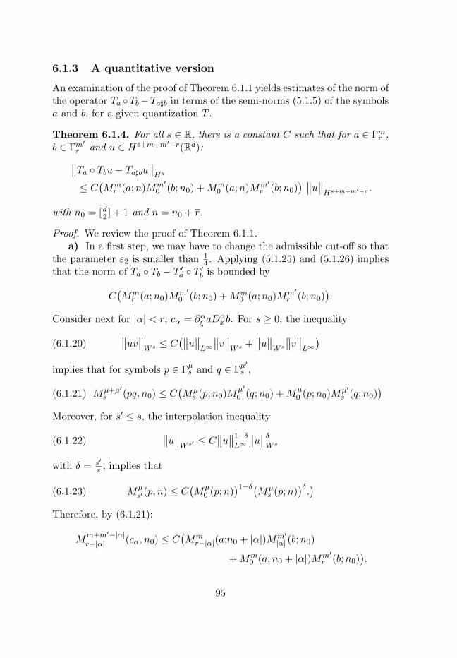
Para-differential Calculus and Applications to the Cauchy Problem for Nonlinear Systems Guy M´ etivier Universit´ e Bordeaux 1, IMB UMR CNRS 5251 33405 Talence Cedex, France [email protected]May 9, 2008
Transcript
Para-differential Calculus and
Applications to the Cauchy Problem
for Nonlinear Systems
Guy Metivier
Universite Bordeaux 1, IMB UMR CNRS 525133405 Talence Cedex, France
4.1.1 Smoothing and approximation. . . . . . . . . . . . . 514.1.2 The Littlewood-Paley decomposition in Hs. . . . . . 544.1.3 The Littlewood-Paley decomposition in Holder spaces. 58
4.2 The general framework of pseudo-differential operators . . . . 604.2.1 Introduction . . . . . . . . . . . . . . . . . . . . . . . 604.2.2 Operators with symbols in the Schwartz class . . . . . 604.2.3 Pseudo-differential operators of type (1, 1) . . . . . . 634.2.4 Spectral localization . . . . . . . . . . . . . . . . . . . 64
4.3 Action of pseudo-differential operators in Sobolev spaces . . . 654.3.1 Stein’s theorem for operators of type (1, 1) . . . . . . 654.3.2 The case of symbols satisfying spectral conditions . . 69
These notes originate from a graduate course given at the University ofPisa during the spring semester 2007. They were completed while the authorwas visiting the Centro di Ricerca Matematica Ennio De Giorgi in february2008. The author thanks both institutions for their warm hospitality.
The main objective is to present at the level of beginners an introductionto several modern tools of micro-local analysis which are useful for the math-ematical study of nonlinear partial differential equations. The guideline is toshow how one can use the para-differential calculus to prove energy estimatesusing para-differential symmetrizers, or to decouple and reduce systems toequations. In these notes, we have concentrated the applications on the wellposed-ness of the Cauchy problem for nonlinear PDE’s. It is important tonote that the methods presented here do apply to other problems, such as,elliptic equations, propagation of singularities (see the original article of J-M Bony [Bon]), boundary value problems, shocks, boundary layers (see e.g[Me1, Me2, MZ]). In particular, in applications to physical problems, the useof para-differential symmetrizers for boundary value problems is much morerelevant for hyperbolic boundary value problems than for the hyperbolicCauchy problem where there are more direct estimates, relying on symme-try properties that are satisfied by many physical systems. However, theanalysis of boundary value problems involve much more technicalities whichwe wanted to avoid in these introductory lectures. The Cauchy problem isa good warm up to become familiar with the technics.
These notes are divided in three parts. Part I is an introduction toevolution equations. After the presentation of physical examples, we givethe bases of the analysis of systems with constant coefficients. The Fourieranalysis provides both explicit solutions and an exact symbolic calculus forFourier multipliers, which can be used for diagonalizing systems or con-structing symmetrizers. The key word is hyperbolicity. However, we haverestricted the analysis to strongly hyperbolic systems, aiming at simplicity
5
and avoiding the subtleties of weak hyperbolicity.In Part II, we give an elementary and self-contained presentation of the
para-differential calculus which was introduced by Jean-Michel Bony [Bon]in 1979. We start with the Littlewood-Paley or harmonic analysis of classicalfunction spaces (Sobolev spaces and Holder spaces). Next we say a few wordsabout the general framework of the classical pseudo-differential calculus andprove Stein’s theorem for operators of type (1, 1). We go on introducingsymbols with limited smoothness and their para-differential quantization asoperators of type (1, 1). A key idea from J-M.Bony is that one can replacenonlinear expressions, thus nonlinear equations, by para-differential expres-sions, to the price of error terms which are much smoother than the mainterms (and thus presumed to be harmless in the derivation of estimates).These are the para-linearization theorems which in nature are a lineariza-tion of the equations. We end the second part, with the presentation of anapproximate symbolic calculus, which links the calculus of operators to a cal-culus for their symbols. This calculus which generalizes the exact calculusof Fourier multipliers, is really what makes the theory efficient and useful.
Part III is devoted to two applications. First we study quasi-linear hy-perbolic systems. As briefly mentioned in Chapter 1, this kind of systems ispresent in many areas of physics (acoutics, fluid mechanics, electromagntism,elasticity to cite a few). We prove the local well posedness of the Cauchyproblem for quasi-linear hyperbolic systems which admit a frequency de-pendent symmetrizer. This class is more general than the class of systemswhich are symmetric-hyperbolic in the sense of Friedrichs; it also incorpo-rates all hyperbolic systems of constant multiplicity. The key idea is simpleand elementary :
- 1) one looks for symmetrizers (multipliers) which are para-differentialoperators, that means that one looks for symbols;
- 2) one uses the symbolic calculus to translate the desired properties ofthe symmetrizers as operators into properties of their symbols;
- 3) one determines the symbols of the symmetrizers satisfying theseproperties. At this level, the computation is very close to the constantcoefficient analysis of Part I.Though most (if not all) physical examples are symmetric hyperbolic in thesense of Friedrichs, it is important to experiment such methods on the sim-pler case of the Cauchy problem, before applying them to the more delicate,but similar, analysis of boundary value problems where they appear to bemuch more significant for a sharp analysis of the well posed-ness conditions.
The second application concerns the local in time well posedness of theCauchy problem for systems of Schodinger equations, coupled though quasi-
6
linear interactions. These systems arise in nonlinear optics: each equa-tion models the dispersive propagation of the envelop of a high frequencybeam, the coupling between the equations models the interaction betweenthe beams and the coupling is actually nonlinear for intense beams suchas laser beams. This models for instance the propagation of a beam in amedium which by nonlinear resonance create scattered and back-scatteredwaves which interact with the original wave (see e.g. [Blo, Boy, NM, CCM]).It turns out that the system so obtained is not necessarily symmetric so thatthe energy estimates are not obtained by simple and obvious integrationsby part. Here the symbolic calculus helps to understand what is going on.We use the symbolic-paradifferential calculus to decouple the systems andreduce the analysis to scalar equations. At this stage, the para-differentialcalculus can also be used to treat cubic interactions. The stress here thatthe results we give in Chapter 8 are not optimal neither the most generalconcerning Schodinger equations, but they appear as direct applications ofthe calculus developed in Part II. The sharp results require further work(see e.g. [KPV] and the references therein).
7
Part I
Introduction to Systems
8
Chapter 1
Notations and Examples.
This introductory chapter is devoted to the presentation of several classicalexamples of systems which occur in mechanics or physics. From the notionof plane wave, we first present the very important notions of dispersionrelation or characteristic determinant, and of polarization of waves whichare of fundamental importance in physics. From the mathematical point ofview, this yields to introduce the notion of symbol of an equation and tostudy its eigenvalues and eigenvector. We illustrate these notions on theexamples.
1.1 First order systems
1.1.1 Notations
We consider N ×N systems of first order equations
(1.1.1) A0(t, x, u)∂tu+d∑j=1
Aj(t, x, u)∂xju = F (t, x, u)
where (t, x) ∈ R × Rd denote the time-space variables; the Aj are N × Nmatrices and F is a function with values in RN ; they depend on the variables(t, x, u) varying in a subdomain of R× Rd × RN .
The Cauchy problem consists in solving the equation (1.1.1) togetherwith initial conditions
(1.1.2) u|t=0 = h.
9
We will consider only the case of noncharacteristic Cauchy problems, whichmeans that A0 is invertible. The system is linear when the Aj do not dependon u and F is affine in u, i.e. of the form F (t, x, u) = f(t, x) + E(t, x)u.
A very important case for applications is the case of systems of conser-vation laws
(1.1.3) ∂tf0(u) +d∑j=1
∂xjfj(u) = 0.
For smooth enough solutions, the chain rule can be applied and this systemis equivalent to
(1.1.4) A0(u)∂tu+d∑j=1
Aj(u)∂xju = 0
with Aj(u) = ∇ufj(u).
Consider a solution u0 and the equation for small variations u = u0 +εv.Expanding in power series in ε yields at first order the linearized equations:
(1.1.5) A0(t, x, u0)∂tv +d∑j=1
Aj(t, x, u0)∂xjv + E(t, x)v = 0
where
E(t, x, v) = (v · ∇uA0)∂tu0 +d∑j=1
(v · ∇uAj)∂xju0 − v · ∇uF
and the gradients ∇uAj and ∇uF are evaluated at (t, x, u0(t, x)).In particular, the linearized equations from (1.1.3) or (1.1.4) near a con-
stant solution u0(t, x) = u are the constant coefficients equations
(1.1.6) A0(u)∂tu+d∑j=1
Aj(u)∂xju = 0.
1.1.2 Plane waves
Consider a linear constant coefficient system:
(1.1.7) Lu := A0∂tu+d∑j=1
Aj∂xju+ Eu = f
10
Particular solutions of the homogeneous equation Lu = 0 are plane waves:
(1.1.8) u(t, x) = eitτ+ix·ξa
where (τ, ξ) satisfy the dispersion relation :
(1.1.9) det(iτA0 +
d∑j=1
iξjAj + E)
= 0
and the constant vector a satisfies the polarization condition
(1.1.10) a ∈ ker(iτA0 +
d∑j=1
iξjAj + E).
The matrix iτA0 +∑d
j=1 iξjAj + E is called the symbol of L.In many applications, the coefficients Aj and E are real and one is in-
terested in real functions. In this case (1.1.8) is to be replaced by u =Re (eitτ+ix·ξa).
When A0 is invertible, the equation (1.1.9) means that −τ is an eigen-value of
∑ξjA
−10 Aj − iA−1
0 E and the polarization condition (1.1.10) meansthat a is an eigenvector.
In many applications and in particular in the analysis of the Cauchyproblem, one is interested in real wave numbers ξ ∈ Rd. The well posednessfor t ≥ 0 of the Cauchy problem (for instance in Sobolev spaces) depends onthe existence or not of exponentially growing modes eitτ as |ξ| → ∞. Thisleads to the condition, called weak hyperbolicity that there is a constant Csuch that for all ξ ∈ Rd, the roots in τ of the dispersion relation (1.1.9)satisfy Im τ ≥ −C. These ideas are developed in Chapter 2.
The high frequency regime is when |ξ| |E| (assuming that the sizeof the coefficients Aj is ≈ 1). In this regime, a perturbation analysis canbe performed and L can be seen as a perturbation of the homogeneoussystem L0 = A0∂t +
∑Aj∂xj . This leads to the notions of principal symbol
iτA0 +∑d
j=1 iξjAj and of characteristic equation
(1.1.11) det(τA0 +
d∑j=1
ξjAj)
= 0.
Note that the principal symbol and the characteristic equation are homoge-neous in ξ, so that their analysis can be reduced to the sphere |ξ| = 1. In
11
particular, for an homogeneous system L0 weak hyperbolicity means thatfor all ξ ∈ Rd, the roots in τ of the dispersion relation (1.1.11) are real.
However, there are many applications which are not driven by the highfrequency regime |ξ| |E| and where the relevant object is the in-homogeneousdispersion relation (1.1.9). For instance, this is important when one wantsto model the dispersion of light.
1.1.3 The symbol
Linear constant coefficients equations play an important role. First, theyprovide examples and models. They also appear as linearized equations (see(1.1.6)). In the analysis of linear systems
(1.1.12) Lu := A0(t, x)∂tu+d∑j=1
Aj(t, x)∂xju+ E(t, x)u,
and in particular of linearized equations (1.1.5), they also appear by freezingthe coefficients at a point (t, x).
This leads to the important notions of principal symbol of the nonlinearequation (1.1.1)
(1.1.13) L(t, x, u, τ, ξ) := iτA0(t, x, u) +d∑j=1
iξjAj(t, x, u),
and of characteristic equation :
(1.1.14) det(τA0(t, x, u) +
d∑j=1
ξjAj(t, x, u))
= 0,
where the variables (t, x, u, τ, ξ) are seen as independent variables in thephase space R1+d × RN × R1+d.
An important idea developed in these lectures is that many propertiesof the linear equation (1.1.12) and of the nonlinear equation (1.1.1) can beseen on the principal symbol. In particular, the spectral properties of
d∑j=1
ξjA−10 (t, x, u)Aj(t, x, u).
are central to the analysis. Properties such as reality, semi-simplicity, mul-tiplicity of the eigenvalues or smoothness of the eigenvalues and eigenpro-jectors, are crucial in the discussions.
12
1.2 Examples
1.2.1 Gas dynamics
General Euler’s equations
The equations of gas dynamics link the density ρ, the pressure p, the velocityv = (v1, v2, v3) and the total energy per unit of volume and unit of mass Ethrough the equations:
Moreover, E = e+|v|2/2 where e is the specific internal energy. The variablesρ, p and e are linked by a state law. For instance, e can be seen as a functionof ρ and p and one can take u = (ρ, v, p) ∈ R5 as unknowns. The second lawof thermodynamics introduces two other dependent variables, the entropyS and the temperature T so that one can express p, e and T as functionsP, E and T of the variables (ρ, S), linked by the relation
(1.2.2) dE = T dS +Pρ2dρ .
One can choose u = (ρ, v, S) or u = (p, v, S) as unknowns. The equationsread (for smooth solutions):
with ρ and p linked by a state law, p = P(ρ). For instance, p = cργ forperfect gases satisfying (1.2.8).
Acoustics
By linearization of (1.2.12) around a constant state (ρ, v), one obtains theequations
(1.2.13)
(∂t + v · ∇)ρ+ ρdivv = f
ρ(∂t + v · ∇)vj + c2∂jp = gj 1 ≤ j ≤ 3
where c2 := dPdρ
(ρ). Changing variables x to x− tv, reduces to
(1.2.14)
∂tρ+ ρ divv = f
ρ∂tv + c2∇p = g.
1.2.2 Maxwell’s equations
General equations
The general Maxwell’s equations read:
(1.2.15)
∂tD − c curlH = −j,∂tB + c curlE = 0,divB = 0,divD = q
where D is the electric displacement, E the electric field vector, H themagnetic field vector, B the magnetic induction, j the current density andq is the charge density; c is the velocity of light. They also imply the chargeconservation law:
(1.2.16) ∂tq + divj = 0.
To close the system, one needs constitutive equations which link E, D, H,B and j.
15
Equations in vacuum
Consider here the case j = 0 and q = 0 (no current and no charge) and
(1.2.17) D = εE, B = µH,
where ε is the dielectric tensor and µ the tensor of magnetic permeability.In vacuum, ε and µ are scalar and constant. After some normalization
The first two equations imply that ∂tdivE = ∂tdivB = 0, therefore theconstraints divE = divB = 0 are satisfied at all time if they are satisfied attime t = 0. This is why one can “forget” the divergence equation and focuson the evolution equations
(1.2.19)
∂tE − curlB = 0,∂tB + curlE = 0,
Moreover, using that curl curl = −∆Id + grad div, for divergence free fieldsthe system is equivalent to the wave equation :
(1.2.20) ∂2tE −∆E = 0.
In 3× 3 block form, the symbol of (1.2.19) is
(1.2.21) iτ Id + i
(0 Ω−Ω 0
), Ω =
0 −ξ2 ξ3
−ξ3 0 ξ1
ξ2 −ξ1 0
The system is hyperbolic and for ξ 6= 0, the eigenvalues and eigenspaces are
τ = 0, E0 =ξ × E = 0, ξ × B = 0
,(1.2.22)
τ = ±|ξ|, E± =E ∈ ξ⊥, B = ∓ξ × E
|ξ|.(1.2.23)
16
Crystal optics
With j = 0 and q = 0, we assume in (1.2.17) that µ is scalar but that ε is apositive definite symmetric matrix. In this case the system reads:
(1.2.24)
∂t(εE)− curlB = 0,∂tB + curlE = 0,
plus the constraint equations div(εE) = divB = 0 which are again propa-gated from the initial conditions. We choose coordinate axes so that ε isdiagonal:
(1.2.25) ε−1 =
α1 0 00 α2 00 0 α3
with α1 > α2 > α3. Ignoring the divergence conditions, the characteristicequation and the polarization conditions are obtained as solutions of system
(1.2.26) L(τ, ξ)(E
B
):=(τE − ε−1(ξ × B)τB + ξ × E
)= 0 .
For ξ 6= 0, τ = 0 is a double eigenvalue, with eigenspace E0 as in (1.2.22).Note that these modes are incompatible with the divergence conditions. Thenonzero eigenvalues are given as solutions of
E = ε−1(ξ
τ× B) , (τ2 + Ω(ξ)ε−1Ω(ξ))B = 0
where Ω(ξ) is given in (1.2.21). Introduce
A(ξ) := Ω(ξ)ε−1Ω(ξ) =
−α2ξ23 α3ξ1ξ2 α2ξ1ξ3
α3ξ1ξ2 −α1ξ23 − α3ξ
21 α1ξ2ξ3
α2ξ1ξ3 α1ξ2ξ3 −α1ξ22 − α2ξ
21
.
Thendet(τ2 +A(ξ)) = τ2
(τ4 −Ψ(ξ)τ2 + |ξ|2 Φ(ξ)
)with
Ψ(ξ) = (α1 + α2)ξ23 + (α2 + α3)ξ2
1 + (α3 + α1)ξ22
Φ(ξ) = α1α2ξ23 + α2α3ξ
21 + α3α1ξ
22 .
The nonvanishing eigenvalues are solutions of a second order equations inτ2, of which the discriminant is
Ψ2(ξ)− 4|ξ|2Φ(ξ) = P 2 +Q
17
withP = (α1 − α2)ξ2
3 + (α3 − α2)ξ21 + (α3 − α1)ξ2
2
Q = 4(α1 − α2)(α1 − α3)ξ23ξ
22 ≥ 0 .
For a bi-axial crystal ε has three distinct eigenvalues and in general P 2+Q 6=0. In this case, there are four simple eigenvalues
±12
(Ψ±
(P 2 +Q
) 12
) 12.
The corresponding eigenspace is made of vectors (E, B) such that E =ε−1( ξτ × B) and B is an eigenvector of A(ξ).
There are double roots exactly when P 2 +Q = 0, that is when
(1.2.27) ξ2 = 0, α1ξ23 + α3ξ
21 = α2(ξ2
1 + ξ23) = τ2 .
Laser - matter interaction
Still with j = 0 and q = 0 and B proportional to H, say B = H, theinteraction light-matter is described through the relation
(1.2.28) D = E + P
where P is the polarization field. P can be given explicitly in terms of E,for instance in the Kerr nonlinearity model:
(1.2.29) P = |E|2E.
In other models P is given by an evolution equation:
(1.2.30)1ω2∂2t P + P − α|P |2P = γE
harmonic oscillators when α = 0 or anharmonic oscillators when α 6= 0.In other models, P is given by Bloch’s equation which come from a more
precise description of the physical interaction of the light and the electronsat the quantum mechanics level.
With Q = ∂tP , the equations (1.2.15) (1.2.30) can be written as a firstorder 12× 12 system:
(1.2.31)
∂tE − curlB +Q = 0,∂tB + curlE = 0,∂tP −Q = 0,
∂tQ+ ω2P − ω2γE − ω2α|P |2P = 0.
18
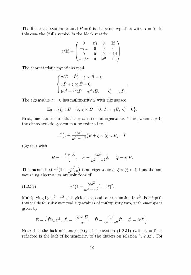
The linearized system around P = 0 is the same equation with α = 0. Inthis case the (full) symbol is the block matrix
iτ Id +
0 iΩ 0 Id−iΩ 0 0 0
0 0 0 −Id−ω2γ 0 ω2 0
.
The characteristic equations readτ(E + P )− ξ × B = 0,
τ B + ξ × E = 0,
(ω2 − τ2)P = ω2γE, Q = iτ P .
.
The eigenvalue τ = 0 has multiplicity 2 with eigenspace
E0 =ξ × E = 0, ξ × B = 0, P = γE, Q = 0
.
Next, one can remark that τ = ω is not an eigenvalue. Thus, when τ 6= 0,the characteristic system can be reduced to
τ2(1 +
γω2
ω2 − τ2
)E + ξ × (ξ × E) = 0
together with
B = −ξ × Eτ
, P =γω2
ω2 − τ2E, Q = iτ P .
This means that τ2(1 + γω2
ω2−τ2
)is an eigenvalue of ξ × (ξ × ·), thus the non
vanishing eigenvalues are solutions of
(1.2.32) τ2(1 +
γω2
ω2 − τ2
)= |ξ|2.
Multiplying by ω2− τ2, this yields a second order equation in τ2. For ξ 6= 0,this yields four distinct real eigenvalues of multiplicity two, with eigenspacegiven by
E =E ∈ ξ⊥, B = −ξ × E
τ, P =
γω2
ω2 − τ2E, Q = iτ P
.
Note that the lack of homogeneity of the system (1.2.31) (with α = 0) isreflected is the lack of homogeneity of the dispersion relation (1.2.32). For
19
wave or Maxwell’s equations, the coefficient n2 in the dispersion relationn2τ2 = |ξ|2 is called the index of the medium. For instance, in vacuum theindex is n0 = 1 with the choice of units made in (1.2.18). Indeed, n
n0is
related to the propagation of light in the medium (whose proper definitionis dτ
d|ξ|). An interpretation of (1.2.32) is that the index and the speed ofpropagation depend on the frequency. In particular, this model can be usedto describe the well known phenomenon of dispersion of light propagatingin glass.
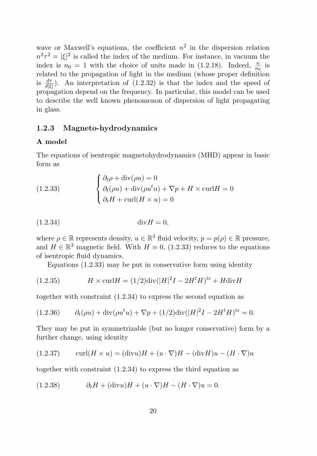
1.2.3 Magneto-hydrodynamics
A model
The equations of isentropic magnetohydrodynamics (MHD) appear in basicform as
where ρ ∈ R represents density, u ∈ R3 fluid velocity, p = p(ρ) ∈ R pressure,and H ∈ R3 magnetic field. With H ≡ 0, (1.2.33) reduces to the equationsof isentropic fluid dynamics.
Equations (1.2.33) may be put in conservative form using identity
(1.2.35) H × curlH = (1/2)div(|H|2I − 2HtH)tr +HdivH
together with constraint (1.2.34) to express the second equation as
with λ = λ− (uξ). The last condition decouples. On the space
(1.2.42) E0(ξ) =ρ = 0, u = 0, H⊥ = 0
,
A is equal to λ0 := u · ξ. From now on we work on E⊥0 = H‖ = 0 which isinvariant by A(U, ξ).
Consider v = H/√ρ, v = H/
√ρ and σ = ρ/ρ. The characteristic system
reads:
(1.2.43)
λσ = u‖
λu‖ = c2σ + v⊥ · v⊥λu⊥ = −v‖v⊥λv⊥ = u‖v⊥ − v‖u⊥
21
Take a basis of ξ⊥ such that v⊥ = (b, 0) and let a = v‖. In such a basis, thematrix of the system reads
(1.2.44) λ− A :=
λ −1 0 0 0 0−c2 λ 0 0 −b 0
0 0 λ 0 a 00 0 0 λ 0 a
0 −b a 0 λ 00 0 0 a 0 λ
The characteristic roots satisfy
(1.2.45) (λ2 − a2)((λ2 − a2)(λ2 − c2)− λ2b2
)= 0 .
Thus, either
λ2 = a2(1.2.46)
λ2 = c2f :=
12
(c2 + h2) +
√(c2 − h2)2 + 4b2c2
)(1.2.47)
λ2 = c2s :=
12
(c2 + h2)−
√(c2 − h2)2 + 4b2c2
)(1.2.48)
with h2 = a2 + b2 = |H|2/ρ.With P (X) = (X−a2)(X− c2)− b2X, P ≤ 0 = [c2
s, c2f ] and P (X) ≤ 0
for X ∈ [min(a2, c2),max(a2, c2)]. Thus,
c2f ≥ max(a2, c2) ≥ a2(1.2.49)
c2s ≤ min(a2, c2) ≤ a2(1.2.50)
1. The case v⊥ 6= 0 i.e. w = ξ × v 6= 0. Thus, the basis such that (1.2.44)holds is smooth in ξ. In this basis, w = (0, b), b = |v⊥| > 0.
1.1 The spaces
E±(ξ) = σ = 0, u‖ = 0, v⊥ ∈ C(ξ × v), u⊥ = ∓v⊥
are invariant for A and
(1.2.51) A = ±a on E± .
22
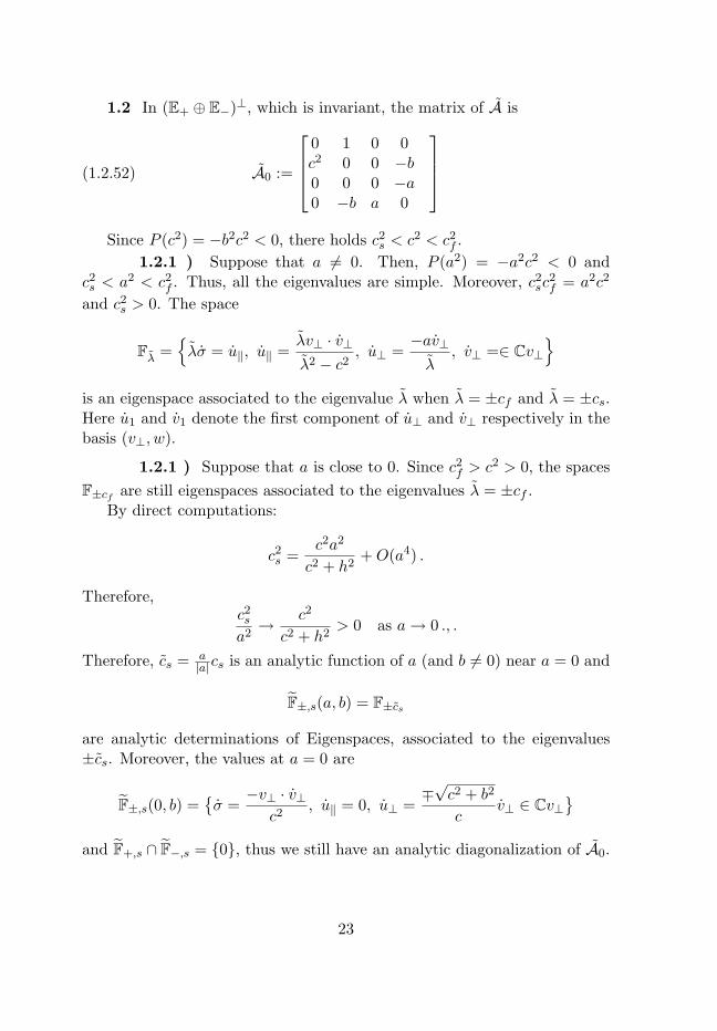
1.2 In (E+ ⊕ E−)⊥, which is invariant, the matrix of A is
(1.2.52) A0 :=
0 1 0 0c2 0 0 −b0 0 0 −a0 −b a 0
Since P (c2) = −b2c2 < 0, there holds c2
s < c2 < c2f .
1.2.1 ) Suppose that a 6= 0. Then, P (a2) = −a2c2 < 0 andc2s < a2 < c2
f . Thus, all the eigenvalues are simple. Moreover, c2sc
2f = a2c2
and c2s > 0. The space
Fλ =λσ = u‖, u‖ =
λv⊥ · v⊥λ2 − c2
, u⊥ =−av⊥λ
, v⊥ =∈ Cv⊥
is an eigenspace associated to the eigenvalue λ when λ = ±cf and λ = ±cs.Here u1 and v1 denote the first component of u⊥ and v⊥ respectively in thebasis (v⊥, w).
1.2.1 ) Suppose that a is close to 0. Since c2f > c2 > 0, the spaces
F±cf are still eigenspaces associated to the eigenvalues λ = ±cf .By direct computations:
c2s =
c2a2
c2 + h2+O(a4) .
Therefore,c2s
a2→ c2
c2 + h2> 0 as a→ 0 ., .
Therefore, cs = a|a|cs is an analytic function of a (and b 6= 0) near a = 0 and
F±,s(a, b) = F±cs
are analytic determinations of Eigenspaces, associated to the eigenvalues±cs. Moreover, the values at a = 0 are
F±,s(0, b) =σ =
−v⊥ · v⊥c2
, u‖ = 0, u⊥ =∓√c2 + b2
cv⊥ ∈ Cv⊥
and F+,s ∩ F−,s = 0, thus we still have an analytic diagonalization of A0.
23
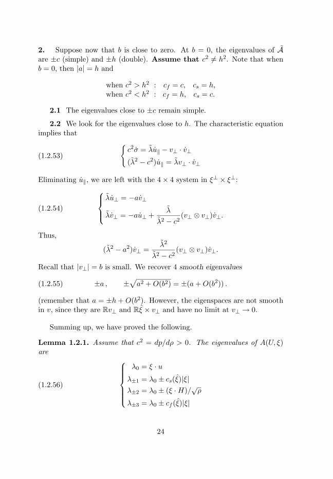
2. Suppose now that b is close to zero. At b = 0, the eigenvalues of Aare ±c (simple) and ±h (double). Assume that c2 6= h2. Note that whenb = 0, then |a| = h and
2.2 We look for the eigenvalues close to h. The characteristic equationimplies that
(1.2.53)
c2σ = λu‖ − v⊥ · v⊥(λ2 − c2)u‖ = λv⊥ · v⊥
Eliminating u‖, we are left with the 4× 4 system in ξ⊥ × ξ⊥:
(1.2.54)
λu⊥ = −av⊥
λv⊥ = −au⊥ +λ
λ2 − c2(v⊥ ⊗ v⊥)v⊥.
Thus,
(λ2 − a2)v⊥ =λ2
λ2 − c2(v⊥ ⊗ v⊥)v⊥.
Recall that |v⊥| = b is small. We recover 4 smooth eigenvalues
(1.2.55) ±a , ±√a2 +O(b2) = ±(a+O(b2)) .
(remember that a = ±h+O(b2). However, the eigenspaces are not smoothin v, since they are Rv⊥ and Rξ × v⊥ and have no limit at v⊥ → 0.
Summing up, we have proved the following.
Lemma 1.2.1. Assume that c2 = dp/dρ > 0. The eigenvalues of A(U, ξ)are
(1.2.56)
λ0 = ξ · uλ±1 = λ0 ± cs(ξ)|ξ|λ±2 = λ0 ± (ξ ·H)/
√ρ
λ±3 = λ0 ± cf (ξ)|ξ|
24
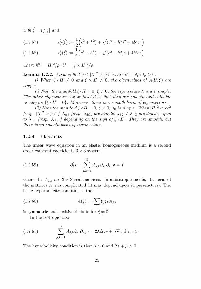
with ξ = ξ/|ξ| and
c2f (ξ) :=
12
(c2 + h2) +
√(c2 − h2)2 + 4b2c2
)(1.2.57)
c2s(ξ) :=
12
(c2 + h2)−
√(c2 − h2)2 + 4b2c2
)(1.2.58)
where h2 = |H|2/ρ, b2 = |ξ ×H|2/ρ.
Lemma 1.2.2. Assume that 0 < |H|2 6= ρc2 where c2 = dp/dρ > 0.i) When ξ · H 6= 0 and ξ × H 6= 0, the eigenvalues of A(U, ξ) are
simple.ii) Near the manifold ξ ·H = 0, ξ 6= 0, the eigenvalues λ±3 are simple.
The other eigenvalues can be labeled so that they are smooth and coincideexactly on ξ ·H = 0. Moreover, there is a smooth basis of eigenvectors.
iii) Near the manifold ξ×H = 0, ξ 6= 0, λ0 is simple. When |H|2 < ρc2
[resp. |H|2 > ρc2 ], λ±3 [resp. λ±1] are simple; λ+2 6= λ−2 are double, equalto λ±1 [resp. λ±3 ] depending on the sign of ξ · H. They are smooth, butthere is no smooth basis of eigenvectors.
1.2.4 Elasticity
The linear wave equation in an elastic homogeneous medium is a secondorder constant coefficients 3× 3 system
(1.2.59) ∂2t v −
3∑j,k=1
Aj,k∂xj∂xkv = f
where the Aj,k are 3 × 3 real matrices. In anisotropic media, the form ofthe matrices Aj,k is complicated (it may depend upon 21 parameters). Thebasic hyperbolicity condition is that
(1.2.60) A(ξ) :=∑
ξjξkAj,k
is symmetric and positive definite for ξ 6= 0.In the isotropic case
(1.2.61)3∑
j,k=1
Aj,k∂xj∂xkv = 2λ∆xv + µ∇x(divxv).
The hyperbolicity condition is that λ > 0 and 2λ+ µ > 0.
25
Chapter 2
Constant CoefficientSystems. Fourier Synthesis
In this chapter, we review the resolution of constant coefficient equations byFourier synthesis. Our first objective is to give an obvious sufficient condition(Assumption 2.1.8) for the well posed-ness of the Cauchy problem in L2 orHs (Theorem 2.1.9). The second important content of the chapter is theintroduction of the notion of hyperbolicity, from an analysis of the generalcondition. Next, we briefly discuss. different notions of hyperbolicity, butwe confine ourselves to the elementary cases.
2.1 The method
In this chapter, we consider equations (or systems)
(2.1.1)∂tu+A(∂x)u = f on [0, T ]× Rd,u|t=0 = h on Rd.
where A is a differential operator (or system) with constant coefficients :
(2.1.2) A(∂x) =∑
Aα∂αxu
2.1.1 The Fourier transform
Notations 2.1.1. The (spatial) Fourier transform F is defined for u ∈ L1(Rd)by
(2.1.3) Fu(ξ) =∫
Rde−ix·ξu(x)dx.
26
We also use the notations u(ξ) for the Fourier transform Fu(ξ). If u ∈L1(Rd) the inverse transformation F−1 is:
(2.1.4) F−1u(x) =1
(2π)n
∫Rdeix·ξu(ξ)dξ.
We denote by S (Rd) the Schwartz class, by S ′(Rd) the space of tem-perate distributions and by E ′(Rd) the space of distributions with compactsupport.
Theorem 2.1.2 (Reminders).i) F is a one to one mapping from the Schwartz class S (Rd) onto itself
with reciprocal F−1.ii) F and F−1 extend as bijections from the space of temperate distri-
butions S ′(Rd) onto itself. Moreover, for u ∈ S ′ and v ∈ S there holds
(2.1.5)⟨u, v⟩
S ′×S=⟨u, v⟩
S ′×S
iii) Plancherel’s theorem : F is an isomorphism from L2 onto itself and
v) For s ∈ R, Hs(Rd) is the space of temperate distributions u such that(1 + |ξ|2)s/2u ∈ L2(Rd). It is an Hilbert space equipped with the norm
(2.1.10)∥∥u∥∥2
Hs =1
(2π)n
∫Rd
(1 + |ξ|2)s|u(ξ)|2dξ.
Combining ii) and iii) implies that for u ∈ S ′ and v ∈ S there holds
(2.1.11)⟨u, v⟩
S ′×S=
1(2π)d
⟨u, v⟩
S ′×S
The spectrum of u is the support of u.
27
When u also depends on time, we let F act for all fixed t and use thefollowing notations:
Notations 2.1.3. If u is a continuous (or measurable) function of time withvalues in a space of temperate distributions, u or Fu denotes the functiondefined for all (or almost all) t by
u(t, ξ) = F (u(t, ·))(ξ).
In particular, the identity
(2.1.12)⟨u, v⟩
S ′×S=⟨u, v⟩
S ′×S
is satisfied for u ∈ S ′(R1+d) and v ∈ S (R1+d).
2.1.2 Solving the evolution equation (2.1.1)
Lemma 2.1.4. If u ∈ S ′(Rd) then
(2.1.13) A(∂x)u(ξ) = A(iξ)u(ξ), A(ξ) =∑
Aα(iξ)α.
Remark 2.1.5. In the scalar case, this means that F diagonalizes A(∂x),with eigenfunctions x 7→ eiξ·x and eigenvalues A(iξ):
A(∂x)eiξ·x = A(iξ)eiξ·x.
For systems, there is a similar interpretation.
Using (2.1.12) immediately implies the following:
Lemma 2.1.6. If u ∈ L1(]0, T [;Hs(Rd)), then in the sense of distributions,
(2.1.14) ∂tu(t, ξ) = ∂tu(t, ξ).
Corollary 2.1.7. For u ∈ C0([0, T ];Hs(Rd)) and f ∈ L1([0, T ];Hs′(Rd)),the equation (2.1.1) is equivalent to
(2.1.15)
∂tu+A(iξ)u = f on [0, T ]× Rd,
u|t=0 = h on Rd.
The solution of (2.1.15) is
(2.1.16) u(t, ξ) = e−tA(iξ)h(ξ) +∫ t
0e(t′−t)A(iξ)f(t′, ξ)dt′.
28
Question : show that the right hand side of (2.1.16) defines a temperatedistribution in ξ. If this is correct, then the inverse Fourier transform definesa function u with values in S ′, which by construction is a solution of (2.1.1).
This property depends on the behavior of the exponentials e−tA(iξ) when|ξ| → ∞. The simplest case is the following:
Assumption 2.1.8. There is a function C(t) bounded on all interval [0, T ],such that
(2.1.17) ∀t ≥ 0, ∀ξ ∈ Rd∣∣e−tA(iξ)
∣∣ ≤ C(t).
Theorem 2.1.9. Under the Assumption 2.1.8, for h ∈ Hs(Rd) and f ∈L1([0, T ];Hs(Rd)), the formula (2.1.16) defines a fonction u ∈ C0([0, T ];Hs(Rd)which satisfies (2.1.1) together with the bounds
Thus, by Lebesgues’ dominated convergence theorem, if h ∈ L2, the mappingt 7→ u0(t, ·) = u0(t, ·) = e−tA(i·)h(·) is continuous from [0,+∞[ to L2(Rd).Thus, u0 = F−1u ∈ C0([0,+∞[;L2(Rd). Moreover:∥∥u(t)
∥∥L2 =
1√(2π)n
∥∥u(t)∥∥L2 ≤
C(t)√(2π)n
∥∥h∥∥L2 = C(t)
∥∥h∥∥L2 .
Similarly, the function v(t, t′, ξ) = e(t′−t)A(iξ)f(t′, ξ) satisfies∥∥v(t, t′, ·)∥∥L2 ≤ C(t− f ′)
∥∥f(t′, ·)∥∥L2 .
Therefore, Lebesgues’ dominated convergence theorem implies that
u1(t, ξ) =∫ t
0v(t, t′, ξ)dt′
belongs to C0([0, T ];L2(Rd)) and satisfies∥∥u1(t)∥∥L2 ≤
∫ t
0C(t− t′)
∥∥f(t′)∥∥L2dt
′.
Taking the inverse Fourier transform, u1 = F−1u1 belongs to C0([0, T ];L2(Rd))and satisfies ∥∥u1(t)
∥∥L2 ≤
∫ t
0C(t− t′)
∥∥f(t′)∥∥L2dt
′.
There are completely similar estimates in Hs. Adding u0 and u1, the theo-rem follows.
29
2.2 Examples
2.2.1 The heat equation
It reads
(2.2.1) ∂tu−∆xu = f, u|t=0 = h.
On the Fourier side, it is equivalent to
(2.2.2) ∂tu+ |ξ|2u = f , u|t=0 = h.
and the solution is
(2.2.3) u(t, ξ) = e−t|ξ|2h(ξ) +
∫ t
0e(t′−t)|ξ|2 f(t′, ξ)dt′.
Remark 2.2.1. The Theorem 2.1.9 can be applied, showing that the Cauchyproblem is well posed. However, it does not give the optimal results : thesmoothing properties of the heat equation can be also deduced from theexplicit formula (2.2.3), using the exponential decay of e−t|ξ|
2as |ξ| → ∞,
while Theorem 2.1.9 only uses that it is uniformly bounded.
2.2.2 Schrodinger equation
A basic equation from quantum mechanics is:
(2.2.4) ∂tu− i∆xu = f, u|t=0 = h.
Note that this equation is also very common in optics and in many otherfields, as it appears as a canonical model in the so-called paraxial approxi-mation, used for instance to model the dispersion of light along long propa-gations.
The Fourier transform of (2.2.4) reads
(2.2.5) ∂tu− i|ξ|2u = f , u|t=0 = h.
The solution is
(2.2.6) u(t, ξ) = eit|ξ|2h(ξ) +
∫ t
0e(t−t′)|ξ|2 f(t′, ξ)dt′.
Since∣∣eit|ξ|2∣∣ = 1, the Theorem 2.1.9 can be applied, both for t ≥ 0 and
t ≤ 0, showing that the Cauchy problem is well posed in Sobolev spaces.
Theorem 2.2.2. For h0 ∈ Hs+1(Rd), h1 ∈ Hs(Rd) and f ∈ L1([0, T ];Hs(Rd)),(2.1.16) defines u ∈ C0([0, T ];Hs+1(Rd) such that ∂tu ∈ C0([0, T ];Hs+1(Rd),u is a solution of (2.2.7) and
(2.2.10)
∥∥u(t)∥∥Hs+1 ≤
∥∥h0
∥∥Hs+1 + 2(1 + t)
∥∥h1
∥∥Hs
+ 2(1 + t)∫ t
0
∥∥f(t′)∥∥Hsdt
′.
(2.2.11)∥∥∂tu(t), ∂xju(t)
∥∥Hs ≤
∥∥h0
∥∥Hs+1 +
∥∥h1
∥∥Hs+1 +
∫ t
0
∥∥f(t′)∥∥Hsdt
′.
Preuve. The estimates (2.2.10) follow from the inequalities
Bounding | sin | and | cos | by 1 implies the estimates (2.2.11) for ∂tu. Simi-larly, the Fourier transform of vj = ∂xju is
(2.2.14)vj(t, ξ) = iξj cos(t|ξ|)h0(ξ)+i
ξj sin(t|ξ|)|ξ|
h1(ξ)
+ i
∫ t
0
ξj sin((t− t′)|ξ|)|ξ|
f(t′, ξ)dt′.
31
Since | sin |, | cos | and |ξj ||ξ| are bounded by 1, this implies that ∂xju satisfies(2.2.11).
2.3 First order systems: hyperbolicity
2.3.1 The general formalism
Consider a N ×N systems
(2.3.1) ∂tu+n∑j=1
Aj∂xju = f, u|t=0 = h,
where u(t, x), f(t, x) et h(x) take their values in RN (or CN ). The coordi-nates are denoted by (u1, . . . , uN ), (f1, . . . , fN ), (h1, . . . , hN ). The Aj areN ×N constant matrices.
After Fourier transform the system reads:
(2.3.2) ∂tu+ iA(ξ)u = f , u|t=0 = h,
with
(2.3.3) A(ξ) =n∑j=1
ξjAj .
The solution of (2.3.2) is given by
(2.3.4) u(t, ξ) = e−itA(ξ)h(ξ) +∫ t
0ei(t′−t)A(ξ)f(t′, ξ)dt′.
2.3.2 Strongly hyperbolic systems
Following the general discussion, the problem is to give estimates for theexponentials e−itA(ξ) = eiA(−tξ). The next lemma is immediate.
Lemma 2.3.1. For the exponential eiA(ξ) to have at most a polynomialgrowth when |ξ| → ∞, it is necessary that for all ξ ∈ Rd the eigenvalues ofA(ξ) are real.
In this case, the system is said to be hyperbolic.
From Theorem 2.1.9 we know that the problem is easily solved when thecondition (2.1.17) is satisfied. Taking into account the homogeneity of A(ξ),leads to the following definition.
32
Definition 2.3.2. The system (2.3.1) is said to be strongly hyperbolic ifthere is a constant C such that
(2.3.5) ∀ξ ∈ Rd,∣∣eiA(ξ)
∣∣ ≤ C.The norm used on the space of N×N matrices is irrelevant. To fix ideas,
on can equip CN with the usual norm
(2.3.6)∣∣u∣∣ =
( N∑k=1
|uk|2) 1
2.
The associated norm for N ×N matrices M is
(2.3.7)∣∣M ∣∣ = sup
u∈CN ,|u|=1
∣∣Mu∣∣
By homogeneity, (2.3.5) is equivalent to
(2.3.8) ∀t ∈ R, ∀ξ ∈ Rd,∣∣eitA(ξ)
∣∣ ≤ C.Lemma 2.3.3. The system is strongly hyperbolic if and only if
i) for all ξ ∈ Rd the eigenvalues of A(ξ) are real and semi-simple,ii) there is a constant C such that for all ξ ∈ Rd the eigenprojectors
of A(ξ) have a norm bounded by C.
Proof. Suppose that the system is strongly hyperbolic. If A(ξ) has a nonreal or real and not semi-simple eivengalue then eiA(±tξ) is not bounded ast→∞. Thus A satisfies i). Moreover, the eigenprojector associated to theeigenvalue λ is
Π = limT→∞
12T
∫ T
−Te−isλ eiA(sξ) ds .
Thus (2.3.8) implies that |Π| ≤ C.Conversely, if A satisfies i) then
(2.3.9) A(ξ) =∑j
λj(ξ)Πj(ξ)
where the λj ’s are the real eigenvalues with eigenprojectors Πj(ξ). Thus
(2.3.10) eiA(ξ) =∑j
eiλj(ξ)Πj(ξ).
Therefore, ii) implies that |eiA(ξ)| ≤ NC.
33
2.3.3 Symmetric hyperbolic systems
A particular case of matrices with real eigenvalues and bounded exponentialsare real symmetric (or complex self-adjoint). More generally, it is sufficientthat they are self- adjoint for some hermitian scalar product on CN .
Definition 2.3.4. i) The system (2.3.1) is said to be hyperbolic symmetricif for all j the matrices Aj are self adjoint.
ii) The system (2.3.1) is said to be hyperbolic symmetrizable if there existsa self-adjoint matrix S, positive definite, such that for all j the matrices SAjare self adjoint.
In this case S is called a symmetrizer.
Theorem 2.3.5. If the system is hyperbolic symmetrizable it is stronglyhyperbolic.
Proof. a) If S is self-adjoint, there is a unitary matrix Ω such that
Because the λk are real, eitD and hence eitS are unitary. In particular,∣∣eitS∣∣ = 1.b) If the system is symmetric, then for all ξ ∈ Rd, A(ξ) is self adjoint.
Thus
(2.3.12)∣∣eiA(ξ)
∣∣ = 1.
c) Suppose that the system is symmetrizable, with symmetrizer S. SinceS is definite positive, its eigenvalues are positive. Using (2.3.11), this allowsto define
(2.3.13) S12 = Ω−1D
12 Ω, D
12 = diag(
√λ1, . . . ,
√λN ).
There holds
(2.3.14) A(ξ) = S−12S−
12SA(ξ)S−
12S
12 = S−
12B(ξ)S
12 .
Thus A(ξ) is conjugated to B(ξ) and
(2.3.15) eiA(ξ) = S−12 eiB(ξ)S
12 .
34
Since SA(ξ) is self-adjoint, B(ξ) = S−12SA(ξ)S−
12 is also self-adjoint and∣∣eiB(ξ)
∣∣ = 1. Therefore,
(2.3.16)∣∣eiA(ξ)
∣∣ ≤ ∣∣S− 12
∣∣ ∣∣S 12
∣∣implying that (2.3.5) is satisfied.
Example 2.3.6. Maxwell equations, linearized Euler equations, equations ofacoustics, linearized MHD introduced in Chapter 1 are hyperbolic symmetricor symmetrizable.
Property i) in Lemma 2.3.3 says that for all ξ, A(ξ) has only real eigenvaluesand can be diagonalized. This does not necessarily imply strong hyperbol-icity: the existence of a uniform bound for the eigenprojectors for |ξ| = 1is a genuine additional condition. For extensions to systems with variablecoefficients, an even stronger condition is required :
Definition 2.3.7. The system (2.3.1) is said to be smoothly diagonalizableis there are real valued λj(ξ) and projectors Πj(ξ) which are real analyticfunctions of ξ on the unit sphere, such that A(ξ) =
∑λj(ξ)Πj(ξ).
In this case, continuity of the Πj implies boundedness on Sd−1 and there-fore:
Lemma 2.3.8. If (2.3.1) is smoothly diagonalizable, then it is strongly hy-perbolic.
Definition 2.3.9. The system (2.3.1) is said to be strictly hyperbolic if forall ξ 6= 0, A(ξ) has N distinct real eigenvalues.
It is said to be hyperbolic with constant multiplicities if for all ξ 6= 0, A(ξ)has only real semi-simple eigenvalues which have constant mutliplicities.
In the strictly hyperbolic case, the multiplicities are constant and equalto 1. Standard perturbation theory of matrices implies that eigenvalues oflocal constant multiplicity are smooth (real analytic) as well as the corre-sponding eigenprojectors. Therefore:
Lemma 2.3.10. Hyperbolic systems with constant multiplicities, and in par-ticular strictly hyperbolic systems, are smoothly diaganalizable and thereforestrongly hyperbolic.
35
2.3.5 Existence and uniqueness for strongly hyperbolic sys-tems
Applying Theorem 2.1.9 immediately implies the following result.
Theorem 2.3.11. If (2.3.1) is strongly hyperbolic, in particular if it is hy-perbolic symmetrizable, then for all h ∈ Hs(Rd) and f ∈ L1([0, T ];Hs(Rd)),(2.3.4) defines u ∈ C0([0, T ];Hs(Rd) which satisfies (2.3.1) and the esti-mates
(2.3.17)∥∥u(t)
∥∥Hs ≤ C
∥∥h∥∥Hs + C
∫ t
0
∥∥f(t′)∥∥Hsdt
′.
2.4 Higher order systems
The analysis of Section 1 can be applied to all systems with constant coef-ficients. We briefly study two examples.
2.4.1 Systems of Schrodinger equations
Extending (2.2.4), consider a N ×N system
(2.4.1) ∂tu− i∑j,k
Aj,k∂xj∂xku+∑j
Bj∂xju = f, u|t=0 = h.
On the Fourier side, it reads:
(2.4.2) ∂tu+ iP (ξ)u = f , u|t=0 = h
with
(2.4.3) P (ξ) :=∑j,k
ξjξkAj,k +∑j
ξjBj := A(ξ) +B(ξ).
The Assumption 2.1.8 is satisfied when there are C and γ such that for t > 0and ξ ∈ Rd:
(2.4.4)∣∣e−itP (ξ)
∣∣ ≤ Ceγt.Case 1 : B = 0. Then P (ξ) = A(ξ) is homogeneous of degree 2 and the
discussion can be reduced to the sphere |ξ| = 1. Again, a necessary andsufficient condition is that the eigenvalues of A(ξ) are real, semi-simple andthe eigenprojectors are uniformly bounded.
36
Case 2 : B 6= 0. The discussion of (2.4.4) is much more delicatesince the first order perturbation B can induce perturbations of order O(|ξ|)in the spectrum of A. For instance, in the scalar case (N = 1), P (ξ) =A(ξ) +B(ξ) ∈ C and a necessary and sufficient condition for (2.4.4) is thatfor all ξ, A(ξ) and B(ξ) are real.
When N ≥ 2, a sufficient condition is that A and B are real symmet-ric (or self-adjoint), since then eitP (ξ) is unitary. In the general case, |ξ|large, the spectrum of P (ξ) is a perturbation of the spectrum of A(ξ) andtherefore a necessary condition is that the eigenvalues of A(ξ) must be real.Suppose the eigenvalues of that A(ξ) have constant multiplicity so that A(ξ)is smoothly diagonalizable:
(2.4.5) A(ξ) =∑
λj(ξ)Πj(ξ)
where the distinct eigenvalue λj are smooth and homogeneous of degree 2and the eigenprojectors Πj are smooth and homogeneous of degree 0. Then,for ξ large, one can block diagonalize P : with
(2.4.6) Ω = Id +∑j 6=k
(λk − λj)−1ΠjBΠk = Id +O(|ξ|−1)
there holds
(2.4.7) Ω−1PΩ =∑
λjΠj + ΠjBΠj +O(1).
Therefore, for (2.4.4) to be valid, it is necessary and sufficient that for all j:i) λj is real,ii) eitΠjBΠj is bounded.
This discussion is made in more details in Part III and extended tosystems with variable coefficients.
This implies that that Cauchy problem for (2.4.8) is well posed in Sobolevspaces, in the spirit of Theorem 2.2.2.
38
Chapter 3
The Method of Symmetrizers
In this chapter, we present the general principles of the method of proof ofenergy estimates using multipliers. To illustrate the method, we apply itto case of constant coefficient hyperbolic systems, where the computationsare simple, explicit and exact. Of course, in this case, the estimates forthe solutions were already present in the previous chapter, obtained fromexplicit representations of the solutions using Fourier synthesis. These ex-plicit formula do not extend (easily) to systems with variable coefficients,while the method of symmetrizers does. In this respect, this chapter is anintroduction to Part III. The constant coefficients computations will serveas a guideline in the more complicated case of equations with variable coef-ficients, to construct symbols, which we will transform into operators usingthe calculus of Part II.
3.1 The method
Consider an equation or a system
(3.1.1)∂tu+A(t)u = f on [0, T ]× Rd,u|t=0 = h on Rd.
where A(t) = A(t, x, ∂x) is a differential operator in x depending on time:
(3.1.2) A(t, x, ∂x) =∑
Aα(t, x)∂αxu
The “method” applies to abstract Cauchy problems (3.1.1) where u andf are functions of time t ∈ [0,∞[ with values in some Hilbert space Hand A(t) is a C1 family of (possibly unbounded) operators defined on D,
39
dense subspace of H. Typically, for our applications H = L2(Rd; CN ) andD = Hm(Rd) where m is the order of A.
Definition 3.1.1. A symmetrizer is a family of C1 functions t 7→ S(t)with values in the space of bounded operators in H such that there are realnumbers C ≥ c > 0, C1 and λ such that
∀t ∈ [0, T ] , S(t) = S(t)∗ and c Id ≤ S(t) ≤ C Id ,(3.1.3)∀t ∈ [0, T ] ,
∣∣∂tS(t)∣∣ ≤ C1 ,(3.1.4)
∀t ∈ [0, T ] , ReS(t)A(t) ≥ −λId .(3.1.5)
In (3.1.3), S∗(t) is the adjoint operator of S(t). The notation ReT =12(T + T ∗) is used in (3.1.5) for the real part of an operator T . When Tis unbounded, the meaning of ReT ≥ λ, is that all u ∈ D belongs to thedomain of T and satisfies
(3.1.6) Re(Tu, u
)H ≥ −λ|u|
2 ,
where ( · )H is the scalar product in H. The property (3.1.5) has to beunderstood in this sense.
For u ∈ C1([0, T ];D), taking the scalar product of Su with the equation(3.1.1) yields:
(3.1.7)d
dt
(S(t)u(t), u(t)
)H +
(K(t)u(t), u(t)
)H = 2Re
(S(t)f(t), u(t)
)H,
where
(3.1.8) K(t) = 2ReS(t)A(t)− ∂tS(t).
Denote by
(3.1.9) E(u(t)) =(S(t)u(t), u(t)
)H
the energy of u at time t. By (3.1.3),
(3.1.10) c∥∥u(t)
∥∥2
H ≤ E(u(t)) ≤ C∥∥u(t)
∥∥2
H.
Moreover, by Cauchy-Schwarz inequality,
(3.1.11) Re(S(t)f(t), u(t)
)H ≤ E(u(t))
12 E(f(t))
12 .
Similarly, by (3.1.5) and (3.1.4), there holds
(3.1.12)(K(t)u(t), u(t)
)H ≥ −(C1 + 2λ)
∥∥u(t)∥∥2
H ≥ −2γE(u(t))
40
with
(3.1.13) γ =12c
(C1 + 2λ).
Therefore:
(3.1.14)d
dtE(u(t)) ≤ 2γE(u(t)) + 2E(u(t))
12 E(f(t))
12 .
Hence:
Lemma 3.1.2. If S is a symmetrizer, then for all u ∈ C10 ([0,∞[;H) ∩
C0([0,∞[;D) there holds
(3.1.15) E(u(t))12 ≤ eγtE(u(0))
12 +
∫ t
0eγ(t−t′)E(f(t′))
12dt′
where f(t) = ∂tu+A(t)u(t) and γ is given by (3.1.13).
3.2 The constant coefficients case
3.2.1 Fourier multipliers
Consider a constant coefficient system
(3.2.1)∂tu+A(∂x)u = f on [0, T ]× Rd,u|t=0 = h on Rd,
where
(3.2.2) A(∂x) =∑
Aα∂αxu
After spatial Fourier transform, the system reads
(3.2.3)
∂tu+A(iξ)u = f on [0, T ]× Rd,
u|t=0 = h on Rd.
It is natural to look for symmerizers that are defined on the Fourier side.
Proposition 3.2.1. Suppose that p(ξ) is a measurable function on Rd suchthat for some m ∈ R:
(3.2.4) (1 + |ξ|2)−m2 p ∈ L∞(Rd).
41
Then the operator
(3.2.5) p(Dx)u := F−1(pu)
is bounded from Hs(Rd) to Hs−m(Rd) for all s and
(3.2.6)∥∥p(Dx)u
∥∥Hs−m ≤
∥∥(1 + |ξ|2)−m2 p∥∥L∞
∥∥u∥∥Hs .
This extends immediately to vector valued functions and matrices p.
Definition 3.2.2. A function p satisfying (3.2.4) is called a Fourier multi-plier of order ≤ m and p(Dx) is the operator of symbol p(ξ).
The definition (3.2.5) and Plancherel’s theorem immediately imply thefollowing.
Proposition 3.2.3 (Calculus for Fourier Multipliers). i) If p and q areFourier multipliers, then
(3.2.7) p(Dx) q(Dx) = (pq)(Dx).
ii) Denoting by p∗(ξ) the adjoint of the matrix p(ξ), then the adjoint ofp(Dx) in L2 is
(3.2.8)(p(Dx)
)∗ = p∗(Dx).
iii) If p is a self adjoint matrix of Fourier multipliers, then p(Dx) ≥ cIdin the sense of self adjoints operators in L2 if and only if for all ξ p(ξ) ≥ cIdin the sense of self-adjoint matrices.
An immediate corollary of this calculus is the following
Proposition 3.2.4. For S(Dx) to be a symmetrizer of (3.2.1) it is necessaryand sufficient that there exist constants C ≥ c > 0 and λ such that
∀ξ ∈ Rd , S(ξ) = S(ξ)∗ and c Id ≤ S(ξ) ≤ C Id ,(3.2.9)∀ξ ∈ Rd , ReS(ξ)A(iξ) ≥ −λId .(3.2.10)
3.2.2 The first order case
Consider a N ×N first order system:
(3.2.11) Lu := ∂tu+d∑j=1
Aj∂xju
42
Theorem 3.2.5. i) The system L has a symmetrizer S(Dx) associated to aFourier multiplier S(ξ) homogeneous of degree 0 if and only if it is stronglyhyperbolic.
ii) The symbol S can be taken constant independent of ξ if and only ifthe system is symmetrizable.
Proof. If S(ξ) satisfies (3.2.10), then by homogeneity and evenness
(3.2.12) Im(S(ξ)A(ξ)
)= 0 i.e.
(S(ξ)A(ξ)
)∗ = S(ξ)A(ξ).
This means that A(ξ) is self-adjoint with respect to the scalar product as-sociated to S(ξ). Thus the eigenvalues of A(ξ) are real and semi-simple andthe eigenprojectors are of norm ≤ 1 in this hermitian structure. By (3.2.9),they are uniformly bounded.
Conversely, if L is strongly hyperbolic then
(3.2.13) A(ξ) =∑
λj(ξ)Πj(ξ), Id =∑
Πj(ξ)
where the λj are real and the Πj are uniformly bounded projectors suchthat ΠjΠk = δj,kΠj . The matrix
(3.2.14) S(ξ) =∑
Π∗jΠj(ξ)
is self-adjoint and
(3.2.15) S(ξ)A(ξ) =∑j,k
λj(ξ)Π∗kΠk(ξ)Πj(ξ) =∑j
λj(ξ)Π∗j (ξ)Πj(ξ)
is self-adjoint. Moreover, since |u| ≤∑|Πju|,
1N|u|2 ≤
∑|Πju|2 = Su · u ≤ N max |Πj |2|u|2
thus S satisfies (3.2.9).Property ii) is just a rephrasing of the definition of symmetrizability.
3.3 Hyperbolic symmetric systems
In this section, we briefly discuss the case of symmetric hyperbolic systems,as a first application of the method of symmetrizers.
43
3.3.1 Assumptions
Consider a first order N ×N linear system:
(3.3.1) ∂tu+d∑j=1
Aj(t, x)∂xju+B(t, x)u = f, u|t=0 = h,
Assumption 3.3.1. The coefficients of the matrices Aj are of class C1,bounded with bounded derivatives on [0, T ] × Rd. The coefficients of B arebounded on [0, T ]× Rd.
Assumption 3.3.2. There is a matrix S(t, x) such that- its coefficients are of class C1, bounded with bounded derivatives
on [0, T ]× Rd.- for all (t, x) ∈ [0, T ]× Rd, S(t, x) is self-adjoint and positive defi-
nite,- S−1 is bounded on [0, T ]× Rd,- for all j and all (t, x) ∈ [0, T ] × Rd, the matrices SAj are self-
adjoint.
S is called a symmetrizer.Maxwell equations or equations of acoustics presented in Chapter 1 are
examples of symmetric systems.Until the end of this section, the Assumptions 3.3.1 and 3.3.2 are sup-
posed to be satisfied.
3.3.2 Existence and uniqueness
We give here without proof the classical existence and uniqueness theoremconcerning hyperbolic-symmetric systems (see [Fr1, Fr2]). For a proof, werefer to Chapter 6.
Theorem 3.3.3. For h ∈ L2(Rd) and t f ∈ L1([0, T ];L2(Rd)), the Cauchyproblem (3.3.1) has a unique solution u ∈ C0([0, T ];L2(Rd).
Moreover, there is C independent of the data f and h, such that for allt ∈ [0, T ]:
(3.3.2)∥∥u(t)
∥∥L2 ≤ C
∥∥h∥∥L2 + C
∫ t
0
∥∥f(t′)∥∥L2dt
′.
44
3.3.3 Energy estimates
We use the method of symmetrizers to prove energy estimates for the (smooth)solutions of (3.3.1). As shown in Chapter 6, these estimates are the key pointin the proof of Theorem 3.3.3.
For simplicity, we assume that the coefficients of the equations and ofthe symmetrizer are real and we restrict ourselves to real valued solutions.We denote by u · v the scalar product of u and v taken in RN .
In many applications, for a function u with values in RN , the S(t, x)u(t, x))·
u(t, x) often corresponds to an energy density. It satisfies:
Lemma 3.3.4. For u ∈ C1, there holds
(3.3.3) ∂t(Su · u) +d∑j=1
∂xj (SAju · u) = 2Sf · u+ 2Ku · u
with
f = ∂tu+d∑j=1
SAj∂xju+Bu(3.3.4)
K = ∂tS +d∑j=1
∂xj (SAj)− SB.(3.3.5)
Proof. The chain rule implies
∂(Gu · u) = (G∂u) · u+Gu · (∂u) + (∂G)u · u.
When G is real symmetric, the first two terms are equal. Using this identityfor G = S, ∂ = ∂t and G = SAj , ∂ = ∂xj implies (3.3.4).
Consider a domain Ω ⊂ [0, T ] × Rd. Denote by Ωτ the truncated sub-domain Ωτ = Ω ∩ t ≤ τ and by ωt the slices ωt = x : (t, x) ∈ Ω. Theboundary of Ωτ is made of the upper and lower slices ωτ and ω0 and of alateral boundary Στ .
For instance when Ω is a cone
(3.3.6) Ω =
(t, x) : 0 ≤ t ≤ T, |x|+ µt ≤ R,
for t ≤ minT,R/µ the slices are the balls
(3.3.7) ωt =x : |x| ≤ R− µt
,
45
and the lateral boundary is
(3.3.8) Στ =
(t, x) : 0 ≤ t ≤ τ, |x|+ µt = R
Integrating (3.3.3) over Ωτ , Green’s formula implies that
Lemma 3.3.5. With notations as in Lemma 3.3.4, there holds
(3.3.9)
∫ωτ
Su · udx =∫ω0
Su · udx−∫
Στ
Gu · u dσ
+ 2∫
Ωτ
(Sf · u+Ku · u)dtdx
where dσ is the surface element on Στ and for (t, x) ∈ Στ ,
(3.3.10) G = ν0S +n∑j=1
νjSAj .
where ν = (ν0, ν1, . . . , νn) is the unit outward normal to Στ .
In the computation above, one can take Ω = [0, T ] × Rd. In this casethere is no lateral boundary Σ, but integrability conditions at infinity arerequired. They are satisfied in particular when u has a compact support inx. Therefore
Lemma 3.3.6. For u of class C1 with compact support in [0, T ]×Rd, thereholds
(3.3.11)∫
Rd(Su·u)|t=τdx =
∫Rd
(Su·u)|t=0dx+2∫
[0,τ ]×Rd(Sf ·u+Ku·u)dtdx
This is indeed a particular case of the identity (3.1.7) integrated between0 and τ . Introduce the global energy at time t of u:
(3.3.12) E(t;u) =∫
RdS(t, x)u(t, x) · u(t, x)dx
Theorem 3.3.7. There is a constant C such that for all u of class C1 withcompact support in [0, T ]× Rd, there holds for t ∈ [0, T ]:
(3.3.13) E(t;u)12 ≤ eCtE(0;u)
12 +
∫ t
0eC(t−t′)E(t′; f)dt′.
46
Proof. This is indeed a particular case of Lemma 3.1.2.Since S(t, x) is symmetric definite positive, bounded with bounded in-
verse there are constants m > 0 and M ≥ m such that
The Cauchy-Schwarz inequality implies that for all (t, x) and all vectors kand h :
(3.3.16)∣∣S(t, x)h · k
∣∣ ≤ (S(t, x)h · h) 1
2(S(t, x)k · k
) 12 .
Taking h = f(t, x) and k = u(t, x), integrating x and using the Cauchy-Schwarz inequality for the integral implies that
(3.3.17) ∀t ∈ [0, T ] :∫
Rd(Sf · u)(t, x)dx ≤ E(t; f)
12E(t;u)
12 .
The assumptions imply that the matrix K defined in (3.3.5) is bounded.With (3.3.14), we conclude that there is a constant C such that for all u ∈ C0
with compact support in [0, T ]× Rd, the following estimate is satisfied:
(3.3.18) ∀t ∈ [0, T ] :∫
Rd(Ku · u)(t, x)dx ≤ CE(t;u).
Introduce ϕ(t) = E(t;u)12 and ψ(t) = E(t; f)
12 . The identity (3.3.11) and
the estimates above imply that
(3.3.19) ϕ(t)2 ≤ ϕ(0)2 + 2∫ t
0ψ(t′)ϕ(t′)dt′ + C
∫ t
0ϕ(t′)2dt′.
This integral inequality implies
(3.3.20) ϕ(t) ≤ e12Ctϕ(0) +
∫ t
0e
12C(t−t′)ψ(t′)dt′
that is (3.3.13) with the constant 12C.
Proof of (3.3.20). Let y(t) denote the right hand side of (3.3.19). This is anonnegative nondecreasing function of t. It is differentiable and
y′(t) = 2ψ(t)ϕ(t) + Cϕ(t)2 ≤ 2ψ(t)√y(t) + Cy(t).
47
Thus z(t) = e−Cty(t) satisfies
z′(t) ≤ 2e−Ct ψ(t)√y(t) = 2e−
12Ctψ(t)
√z(t).
Therefore √z(t) ≤
√z(0) +
∫ t
0e−
12Ct′ψ(t′)dt′.
and
ϕ(t) ≤√y(t) ≤ e
12Ct(√
z(0) +∫ t
0e−
12Ct′ψ(t′)dt′
).
Next we turn to local estimates. The key remark is that the boundaryintegral over Στ occurring in (3.3.9) can be made ≥ 0 by choosing properlythe domain Ω. For instance:
Lemma 3.3.8. Consider a cone Ω as in (3.3.6). There is µ0 such that forµ ≥ µ0 the symmetric boundary matrix G given in (3.3.10) is nonnegative.
Proof. The outward unit normal at (t, x) ∈ Σ is
ν0 =µ√
1 + µ2, νj =
1√1 + µ2
xj|x|.
Since S is uniformly definite positive and the SAj are uniformly bounded, itis clear that G = ν0S +
∑nj=1 νjSAj is nonnegative if µ is large enough.
Assuming that µ ≥ µ0, the equality (3.3.9) implies the inequality
(3.3.21)∫ωτ
Su · udx ≤∫ω0
Su · udx+ 2∫
Ωτ
(Sf · u+Ku · u)dtdx
From here, one can repeat the proof of Theorem 3.3.7 and show that thelocal energy
(3.3.22) EΩ(t, u) =∫ωt
S(t, x)u(t, x) · u(t, x) dx
satisfies
Theorem 3.3.9. There is a constant C such that if Ω is the cone (3.3.6)with µ ≥ µ0 and u is of class C1 there holds for t ∈ [0, T ]:
(3.3.23) EΩ(t;u)12 ≤ eCtEΩ(0;u)
12 +
∫ t
0eC(t−t′)EΩ(t′; f)dt′.
In particular, if f = 0 on Ω and u|t=0 = 0 on ω0, then u = 0 on Ω. This isthe key step in the proof of local uniqueness and finite speed of propagationfor hyperbolic symmetric systems.
48
Part II
The Para-DifferentialCalculus
49
Chapter 4
Pseudo-differential operators
This chapter is devoted to a quick presentation of the language of pseudo-differential operators, in the most classical sense. The important points inthis chapter are
- the notion of operators and symbol, with the exact calculus when thesymbol are in the Schwartz class;
- the notion of symbols of type (1, 1) as this is the class where the para-differential calculus takes place;
- Stein’s theorem for the action of operators of type (1, 1);- the crucial notion of spectral condition for the symbols as this is the
key feature of the para-differential symbols;- the extension of Stein’s theorem to such operators.
One key idea, coming from harmonic analysis, is to use in a systematicway the Littlewood-Paley decomposition of functions and operators. Inparticular, we start with a characterization of classical function spaces usingthe Littlewood-Paley analysis.
4.1 Fourier analysis of functional spaces
Notations: Recall that F denotes the Fourier transform acting on temper-ate distributions S ′(Rd). We use its properties listed in Theorem 2.1.2.
The spectrum of u is the support of u.
Fourier multipliers are defined by the formula
(4.1.1) p(Dx)u = F−1(pFu)
provided that the multiplication by p is defined at least form S to S ′. p(Dx)is the operator associated to the symbol p(ξ).
50
Function spaces. Recall the following definitions.
Definition 4.1.1. For s ∈ R, Hs(Rd) is the space of distributions u ∈S ′(Rd) such that their Fourier transform is locally integrable and
(4.1.2)∥∥u∥∥2
Hs(Rd):=
1(2π)d
∫(1 + |ξ|2)s
∣∣u(ξ)∣∣2dξ < +∞.
Definition 4.1.2 (Lipschitz and Holder spaces). i) For m ∈ N we denote byWm,∞(Rd) the space of functions u ∈ L∞(Rd) such that all their derivatives∂αu of order |α| ≤ m belong to L∞(Rd).
ii) For µ ∈]0, 1[, we denote by Wµ,∞(Rd) the space of continuous andbounded functions on Rd such that
(4.1.3)[u]µ
:= sup|u(x)− u(y)||x− y|µ
< +∞.
iii) for µ > 0, µ /∈ N, denoting by [µ] the greatest integer < µ, the spaceWµ,∞(Rd) is the space of functions in W [µ],∞(Rd) such that their derivatives∂αu of order |α| = [µ] belong to Wµ−[µ],∞.
iv) For m ∈ N, Cmb (Rd) denotes the space of functions in Wm,∞(Rd)such that all their derivatives of order ≤ m are continuous.
Remarks 4.1.3. W 1,∞ is the space of bounded and Lipschitz functions onRd, that is which satisfy (4.1.3) with µ = 1.
When µ /∈ N, the notations Wµ,∞ is not quite standard for Holder spaces.However, it is convenient for us to use the unified notations Wµ,∞ for µ ∈ Nand µ /∈ N.
The definition of spaces Wµ,∞ will be extended to µ < 0 (µ /∈ Z) afterProposition 4.1.16
All these spaces are equipped with the obvious norms.
4.1.1 Smoothing and approximation.
We list here several useful lemmas concerning the approximation and theregularization of functions.
We consider in this section families of functions χλ ∈ S (Rd) such that
(4.1.4)
∀(α, β) ∈ Nd × Nd, ∃Cα,β :
∀λ ≥ 1, ∀ξ ∈ Rd :∣∣ξα∂βξ χλ(ξ)
∣∣ ≤ Cα,βλ|α|−|β|.Example 4.1.4. Take χ ∈ S and χλ(ξ) = χ(λ−1ξ).
51
Remark 4.1.5. The condition (4.1.4) is equivalent to the condition thatthe family χλ(ξ) := χλ(λξ) is bounded in S . In the example above χλ = χis fixed.
Let ϕλ = F−1χλ ∈ S (Rd). Then
(4.1.5) χλ(Dx)u(x) =∫u(x− y)ϕλ(y)dy.
The remark above implies that ϕλ(x) = λdϕλ(λx) where ϕλ = F−1χλ isbounded in S . Therefore, there are constants Cα,β such that
(4.1.6)∫ ∣∣xα∂βxϕλ(x)
∣∣dx ≤ Cα,β λ|β|−|α|.Lemma 4.1.6. Suppose that the family χλ satisfies (4.1.4). For all α ∈Nd, there is a constant Cα such that for all λ > 0, the operators ∂αxχλ(Dx)are bounded from Lp(Rd) to Lq(Rd) for 1 ≤ p ≤ q ≤ +∞ with norm lessthan or equal to Cαλ
|α|+ dp− dq .
Proof. ∂αxχλ(Dx)u is the convolution operator by ∂αxϕλ(x) = λd+|α|(∂αx ϕλ(λx).Since ϕλ is bounded in S ,∥∥∂αxϕλ∥∥Lr ≤ Cαλ|α|+d(1− 1
r)
and the lemma follows from Young’s inequality.
Corollary 4.1.7 (Bernstein’s inequalities). Suppose that a ∈ Lp(Rd) has itsspectrum contained in the ball |ξ| ≤ λ. Then a ∈ C∞ and for all α ∈ Nd
and q ≥ p, there is Cα,p,q (independent of λ) such that
(4.1.7) ‖∂αx a‖Lq(Rd) ≤ Cα,p,qλ|α|+ d
p− dq ‖a‖Lp(Rd) .
In particular,
‖∂αx a‖Lp(Rd) ≤ Cαλ|α|‖a‖Lp(Rd), p = 2, p =∞,(4.1.8)
‖a‖L∞(Rd) ≤ Cλd2 ‖a‖L2(Rd)(4.1.9)
Proof. Let χ ∈ C∞0 (Rd) supported in |ξ| ≤ 2 and equal to 1 for |ξ| ≤ 1.Then a = χλa where χλ(ξ) = χ(λ−1ξ). Thus a = χλ(Dx)a and (4.1.7)follows from the previous Lemma.
52
Lemma 4.1.8. Suppose that the family χλ satisfies (4.1.4) and that eachχλ vanishes on a neighborhood of the origin. For µ > 0, there is a constantCµ such that :
for all u ∈Wµ,∞(Rd), one has the following estimate :
(4.1.10)∥∥χλ(Dx)u
∥∥L∞≤ Cµ
∥∥u∥∥Wµ,∞ λ
−µ.
Proof. Note that the estimate follows from Lemma 4.1.6 when λ ≤ 1.Since χλ vanishes in a neighborhood of the origin, there holds∫
yαϕλ(y)dy = Dαξ χλ(0) = 0.
Therefore, (4.1.5) implies that
(4.1.11) χλ(Dx)u(x) =∫ (
u(x− y)−∑|α|<µ
(−y)α
α!∂αxu(x)
)ϕλ(y)dy.
When µ ≤ 1 we use that
(4.1.12)∣∣u(x− y)− u(x)
∣∣ ≤ C∥∥u∥∥Wµ,∞ |y|µ.
When µ > 1, we use Taylor’s formula at order n = µ − 1 when µ ∈ N andat order n = [µ] when µ /∈ N. It implies that
(4.1.13)
u(x− y)−∑|α|<µ
(−y)α
α!∂αxu(x)
=∑|α|=n
(−y)αnα!
∫ 1
0(1− t)n−1
(∂αxu(x− ty)− ∂αxu(x)
)dt
Thus the the integrand in (4.1.11) is O(|y|µ ϕλ(y)‖u‖Wµ,∞
)and therefore
(4.1.14)∣∣ψλ(Dx)u(x)
∣∣ ≤ C∥∥u∥∥Wµ,∞
∫|y|µ|ϕλ(y)|dy.
Together with (4.1.6) this implies (4.1.10).
Lemma 4.1.9. Suppose that the family χλ satisfies (4.1.4) and that eachχλ is equal to 1 on a neighborhood of the origin. For µ > 0, there is aconstant Cµ such that for all u ∈Wµ,∞ :
(4.1.15)∥∥u− χλ(Dx)u
∥∥L∞≤ C
∥∥u∥∥Wµ,∞ λ
−µ
53
Proof. The proof is quite similar. The inverse Fourier transform ϕλ nowsatisfy ∫
ϕλ(y)du = 1 and∫yαϕλ(y)dy = 0 when |α| > 0.
Therefore,
(4.1.16) χλ(Dx)u(x)− u(x) =∫ (
u(x− y)−∑|α|<µ
(−y)α
α!∂αxu(x)
)ϕλ(y)dy.
The end of the proof is identical.
Corollary 4.1.10. For all µ > 0, there is a constant C such that for allλ > 0 and for all a ∈ Wµ,∞ with spectrum contained in |ξ| ≥ λ, one hasthe following estimate :
(4.1.17)∥∥a∥∥
L∞≤ C
∥∥a∥∥Wµ,∞ λ
−µ
Proof. a = a− χ(λ−1Dx)a if χ is equal to 1 near the origin is supported inthe ball of radius 1.
4.1.2 The Littlewood-Paley decomposition in Hs.
Let χ ∈ C∞0 (Rd) satisfy 0 ≤ χ ≤ 1 and
(4.1.18) χ(ξ) = 1 for |ξ| ≤ 1.1 , χ(ξ) = 0 for |ξ| ≥ 1.9 .
For k ∈ Z, let
(4.1.19) χk(ξ) = χ(2−kξ), ψk = χk − χk−1.
Introduce the operators acting on S ′:
(4.1.20) Sku = F−1(χ(2−kξ)u(ξ)
)and ∆k = Sk − Sk−1. In particular
(4.1.21) u = S0u+∞∑k=1
∆ku
54
Proposition 4.1.11. Consider s ∈ R. A temperate distribution u belongsto Hs(Rd) if and only if
i) u0 := S0u ∈ L2(Rd) and for all k > 0, uk := ∆ku ∈ L2(Rd)ii) the sequence δk = 2ks‖uk‖L2(Rd) belongs to `2(N).
Moreover, there is a constant C, independent of u, such that
(4.1.22)1C‖u‖2Hs ≤
(∑k
δ2k
)1/2≤ C‖u‖2Hs
Proof. In the frequency space there holds
(4.1.23) u =∞∑k=1
uk
Let θ0 = χ0 and θk = ψk for k ≥ 1. Because 0 ≤ θk ≤ 1, there holds∑∣∣uk(ξ)∣∣2 =∑
θ2k(ξ)
∣∣u(ξ)∣∣2 ≤∑ θk(ξ)
∣∣u(ξ)∣∣2 =
∣∣u(ξ)∣∣2
On the other hand, every ξ belongs at most to the support of 3 functionsθk. Therefore ∣∣u(ξ)
∣∣2 =∣∣∣∑ uk(ξ)
∣∣∣2 ≤ 3∑∣∣uk(ξ)∣∣2.
Summing up, we have proved that
(4.1.24)∑∣∣uk(ξ)∣∣2 ≤ ∣∣u(ξ)
∣∣2 ≤ 3∑∣∣uk(ξ)∣∣2.
Multiplying by (1 + |ξ|2)s, integrating over Rd, and noticing that
(4.1.25)14
22k ≤ 1 + |ξ|2 ≤ 4 22k on the support of θk,
the proposition follows.
Proposition 4.1.12. Consider s ∈ R and R > 0. Suppose that ukk∈N isa sequence of functions in L2(Rd)such that
i) the spectrum of u0 is contained in the ball |ξ| ≤ R and for k > 0the spectrum of uk is contained in
1R2k ≤ |ξ| ≤ R2k
.
ii) the sequence δk = 2ks‖uk‖L2(Rd) belongs to `2(N).Then u =
∑uk belongs to Hs(Rd) and there is a constant C, independent
of the sequence such that
‖u‖2Hs ≤ C(∑
k
δ2k
)1/2
When s > 0, it is sufficient to assume that the spectrum of uk is containedin the ball
|ξ| ≤ R2k
.
55
Proof. Define the θj as in the previous proof. By Lemma 4.1.6,∥∥θj(Dx)uk∥∥L2 ≤ C
∥∥uk∥∥L2 ≤ C2−ksδk.
Moreover, the spectral assumption in i) implies that θj(Dx)uk = 0 if |k−j| ≥a = ln(2R)/ ln 2. Thus
(4.1.26)∥∥θj(Dx)u
∥∥L2 ≤ C2−jsδj , δj =
∑|k−j|≤a
2s(j−k)δk
When the spectrum of uk is contained in the ball |ξ| ≤ R2k, thenθj(Dx)uk = 0 when j ≥ k+a. Thus the estimate in (4.1.26) is satisfied with
δj =∑k≥j−a
2s(j−k)δk.
When s > 0, we see that this sequence (δj) still belongs to `2 as a conse-quence of Young’s inequality for the convolution of sequences, one in `2, theother in `1.
We will also use another version where the spectral localization is re-placed by estimates which mimic this localization.
Proposition 4.1.13. Let 0 < s and let n be an integer, n > s. There is aconstant C such that :
for all sequence (fk)k≥0 in Hn(Rd) satisfying for all α ∈ Nd of length|α| ≤ n
(4.1.27)∥∥∂αx fk∥∥L2(Rd)
≤ 2k(|α|−s)εk, with (εk) ∈ `2,
the sum f =∑fk belongs to Hs(Rd) and
(4.1.28)∥∥f∥∥2
Hs(Rd)≤ C
∞∑k=0
ε2k.
Proof. Since s > 0, the series∑fk converge in L2(Rd) and f =
∑fk. There
holds ∥∥θj(Dx)fk∥∥L2 ≤ C
∥∥fk∥∥L2 ≤ C2−ksεk,∥∥θj(Dx)fk∥∥L2 ≤ C2−nj
∥∥fk∥∥Hn ≤ C2−ks2n(k−j)εk.
We use the first estimate when j ≤ k and the second when j > k. Therefore,
(4.1.29)∥∥θj(Dx)f
∥∥L2 ≤ C2−js(ε′j + ε′′j )
56
withε′j =
∑k≥j
2(j−k)sεk, ε′′j =∑k<j
2(n−s)(k−j)εk.
Because s < n, (ε′′j ) belongs to `2 and because s > 0, (ε′j) belongs to`2.Moreover, their norms are dominated by the `2 norm of the sequence(εk).
The restriction s > 0 can be dropped when the fk satisfy an appropriatespectral condition.
Proposition 4.1.14. Let s ∈ R, κ > 0 and let n > s be an integer. Thereis a constant C such that :
for all sequence (fk)k≥0 in Hn(Rd) satisfying (4.1.27) and
(4.1.30) suppfk ⊂ ξ : 1 + |ξ| ≥ κ2k,
f =∑fk belongs to Hs(Rd) and satisfies (4.1.28)
Proof. The spectral condition implies that there is N such that θj(Dx)fk = 0when j < k − N . Therefore the estimate (4.1.29) is satisfied with ε′j nowdefined by
ε′j =j+N∑k=j
2(j−k)sεk.
Noticing that this sequence (ε′j) belongs to `2 when (εk) ∈ `2, implies theproposition.
The estimates of ‖∆ku‖L2 can be combined with Lemma 4.1.6. In par-ticular, for u ∈ Hs(Rd) there holds
(4.1.31)∥∥∆ku
∥∥L∞≤ εk2−k(s− d
2)
with εk ∈ `2. Summing in k immediately implies the following results.
Proposition 4.1.15 (Sobolev embeddings). i) If s > d2 , then Hs(Rd) ⊂
L∞(Rd) and there is a constant C such that for u ∈ Hs(Rd):
(4.1.32)∥∥u∥∥
L∞≤ C
∥∥u∥∥Hs .
ii) If s < d2 , there is a constant C such that for u ∈ Hs(Rd) and all k
(4.1.33)∥∥Sku∥∥L∞ ≤ εk2k( d
2−s),
∞∑k=0
ε2k ≤ C
∥∥u∥∥2
Hs .
57
4.1.3 The Littlewood-Paley decomposition in Holder spaces.
Proposition 4.1.16. Consider µ > 0, µ /∈ N. A temperate distribution ubelongs to Wµ,∞(Rd) if and only if
i) u0 := S0u ∈ L∞ and for all k > 0, uk := ∆ku ∈ L∞(Rd)ii) the sequence δk = 2kµ‖uk‖L∞(Rd) belongs to `∞(N).
Moreover, there is a constant C, independent of u, such that
(4.1.34)1C
∥∥u∥∥Wµ,∞ ≤ sup
kδk ≤ C
∥∥u∥∥Wµ,∞
Proof. By Lemma 4.1.6 ∥∥S0u∥∥L∞≤ C
∥∥u∥∥L∞.
The estimate of ∆ku is a particular case of Lemma 4.1.10.Conversely, if ‖uk‖L∞ ≤ C2−kµ, then Lemma 4.1.7 implies that for |α| <
µ, ‖∂αuk‖L∞ ≤ C2−k(µ−|α|). This shows that the series∑∂αuk converges
We use the first estimate when 2−k ≤ |x− y| and the second when |x− y| <2−k. Using that 0 < µ− [µ] < 1, the estimates sums in k and we obtain that∣∣∂αuk(x)− ∂αuk(y)
∣∣ ≤ C ′|x− y|(µ−[µ]),
which proves that u ∈ Cµb .
For µ < 0, µ /∈ Z, we can take the properties i) and ii) as a definition ofthe space Wµ,∞:
Definition 4.1.17. Consider µ < 0, µ /∈ Z. A temperate distribution ubelongs to Wµ,∞(Rd) if and only if
i) u0 := S0u ∈ L∞ and for all k > 0, uk := ∆ku ∈ L∞(Rd)ii) the sequence δk = 2kµ‖uk‖L∞(Rd) belongs to `∞(N).
Using Lemma 4.1.6, one can check that the space does not depend onthe particular choice of the cut-off function defining the Littlewood-Paley de-composition. There are results analogous to Propositions 4.1.12 and 4.1.13,but be omit them.
58
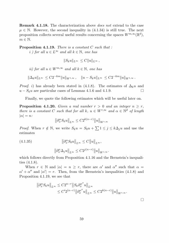
Remark 4.1.18. The characterization above does not extend to the caseµ ∈ N. However, the second inequality in (4.1.34) is still true. The nextproposition collects several useful results concerning the spaces Wm,∞(Rd),m ∈ N.
Proposition 4.1.19. There is a constant C such that :i ) for all u ∈ L∞ and all k ∈ N, one has
Proof. i) has already been stated in (4.1.8). The estimates of ∆ku andu− Sku are particular cases of Lemmas 4.1.6 and 4.1.9.
Finally, we quote the following estimates which will be useful later on.
Proposition 4.1.20. Given a real number r > 0 and an integer n ≥ r,there is a constant C such that for all k, u ∈ W r,∞ and α ∈ Nd of length|α| = n: ∥∥∂αxSku∥∥L∞ ≤ C2k(n−r)∥∥u∥∥
W r,∞
Proof. When r /∈ N, we write Sku = S0u +∑
1 ≤ j ≤ k∆ju and use theestimates
(4.1.35)∥∥∂αxS0u
∥∥L∞≤ C
∥∥u∥∥L∞,∥∥∂αx∆ju
∥∥L∞≤ C2j(n−r)
∥∥u∥∥W r,∞ .
which follows directly from Proposition 4.1.16 and the Bernstein’s inequali-ties (4.1.8).
When r ∈ N and |α| = n ≥ r, there are α′ and α′′ such that α =α′ + α′′ and |α′| = r. Then, from the Bernstein’s inequalities (4.1.8) andProposition 4.1.19, we see that∥∥∂αxSku∥∥L∞ ≤ C2n−r
∥∥Sk∂α′′x u∥∥L∞
≤ C ′2(n−r)∥∥∂α′′x u∥∥L∞≤ C2k(n−r)∥∥u∥∥
W r,∞ .
59
4.2 The general framework of pseudo-differentialoperators
4.2.1 Introduction
Recall that the Fourier multiplier p(Dx) is defined by (4.1.1). It is definedas soon as the multiplication by p acts from S to S ′. The main propertiesof Fourier mulitpliers are that
• p(Dx) q(Dx) = (pq)(Dx),•(p(Dx)
)∗ = (p)(Dx),• if p ≥ 0, then p(Dx) is nonnegative as an operator,
The goal of pseudo-differential calculus is to extend the definition (4.1.1)to symbols p(x, ξ), by the following formula:
(4.2.1)(p(x,Dx)u
)(x) = (2π)−d
∫eix·ξp(x, ξ)u(ξ)dξ ,
and to show that the properties above remain true, not in an exact sensebut up to remainder terms which are smoother.
4.2.2 Operators with symbols in the Schwartz class
As an introduction, we first study the case of operators defined by symbolsin the Schwartz class. The results will be extended to more general symbolsin the following sections.
For p ∈ S (Rd × Rd) and u ∈ S (Rd), p(x, ξ)u(ξ) and eix·ξp(x, ξ)u(ξ)belong to S (Rd×Rd) so that the integral in (4.2.1) is convergent and definesa function in the Schwarz class S (Rd). Substituting the definition of u yieldsthe convergent integral
(2π)−d∫ei(x−y)·ξp(x, ξ)u(y)dξ dy,
so that
(4.2.2)(p(x,Dx)u
)(x) =
∫(F−1
ξ p)(x, x− y)u(y)dy ,
where F−1ξ p ∈ S (Rd × Rd) denotes the inverse Fourier transform of p with
respect to the variables ξ. Thus the kernel K(x, y) = (F−1ξ p)(x, x − y)
belongs to S (Rd × Rd) and this clearly implies :
60
Lemma 4.2.1. If p ∈ S (Rd × Rd), the operator p(x,Dx) extends as acontinuous operator from S ′(Rd) to S (Rd) and for u and v in S ′(Rd):
(4.2.3)⟨p(x, ∂x)v, u
⟩S (Rd)×S ′(Rd =
⟨K,u⊗ v
⟩S (Rr×Rd)×S ′(Rr×Rd)
.
Conversely, for any K ∈ S (Rd×Rd) the symbol p = FzK(x, x−z), thatis
(4.2.4) p(x, ξ) =∫e−iz·ξK(x, x− z)dz,
belongs to S (Rd × Rd). Thus the theory of pseudo-differential operatorswith symbols in the Schwarz class S is nothing but the theory of operatorswith kernels in the Schwarz class.
On the Fourier side, for u ∈ S the Fourier transform of (4.2.1) is givenby the absolutely convergent integral
(2π)−d∫eix·(ξ−η)p(x, ξ)u(ξ)dξ dx,
and therefore
(4.2.5) F(p(x,Dx)u
)(η) = (2π)−d
∫(Fxp)(η − ξ, ξ)u(ξ)dξ ,
where Fxp ∈ S (Rd × Rd) denotes the Fourier transform of p with respectto the variables x.
Lemma 4.2.2. If p and q belong to S (Rd×Rd), then p(x,Dx) q(x,Dx) =r(x,Dx) with
The change of variables z = x+y yields (4.2.6) while the change of variablesζ = ξ′ − ξ yields (4.2.7). Note that all the integrals above are absolutelyconvergent and that r ∈ S (Rd × Rd).
We define (p(x,Dx))∗ as the adjoint of p(x,Dx) acting in L2, that is asthe transposed of p(x, ∂x) for the anti-duality 〈u, v〉:
(4.2.8)⟨(p(x,Dx)
)∗u, v⟩
S×S ′=⟨u, p(x,Dx)v
⟩S ′×S
.
For u and v in S this means that
(4.2.9)∫ (
p(x,Dx))∗u, v dx =
∫u, p(x,Dx)v dx.
Lemma 4.2.3. If p belongs to S (Rd × Rd), then(p(x,Dx)
)∗ = r(x,Dx)with
(4.2.10) r(x, ξ) =1
(2π)d
∫e−iy·η p(x+ y, ξ + η)dydη
and
(4.2.11) (Fxr)(η, ξ) = (Fxp)(η, ξ + η).
Proof. By (4.2.2), p(x,Dx) is defined by the kernel K(x, y) = (F−1ξ p)(x, x−
y) which belongs to the Schwartz class. Its adjoint is defined by the kernelK∗(x, y) = K(y, x) = (F−1
ξ p)(y, x − y). By (4.2.4) it is associated to thesymbol
r(x, ξ) =∫e−iz·ξ(F−1
ξ p)(x− z, z)dz.
Thusr(x, ξ) =
1(2π)d
∫eiz·(η−ξ)p(x− z, η)dzdη
and (4.2.10) follows. Similarly,
(Fxr)(η, ξ) =∫e−i(z·ξ+x·η)(F−1
ξ p)(x− z, z)dz
=∫e−iz·(ξ+η)(F−1
ξ Fxp)(η, z)dzdx = (Fxp)(η, ξ + η).
62
4.2.3 Pseudo-differential operators of type (1, 1)
Definition 4.2.4. For m ∈ R, Sm1,1 is the space of functions p, C∞ onRd × Rd such that for all (α, β) ∈ Nd × Nd, there is Cα,β such that
The best constant in (4.2.12) and (4.2.13) define semi-norms, to thatSm1,1 and Sm1,0 are equipped with natural topologies. In particular, a familyof symbols pk is said to be bounded in Sm1,1 [resp. Sm1,0] if they satisfy theestimates (4.2.12) [resp. (4.2.13) ] with constants Cα,β independent of k.
Examples 4.2.5. • Smooth homogeneous functions of degree m, h(ξ) , aresymbols of degree m for |ξ| ≥ 1. Thus χ(ξ)h(ξ) ∈ Sm1,0 if χ ∈ C∞(Rd) isequal to 1 outside a ball and vanishes near the origin.• If χ ∈ C∞0 (Rd) , then for all λ ≥ 1, χλ(ξ) := χ(λ−1ξ) is a symbol of
degree 0 and the family χλ is bounded in Sm1,0.
For such symbols and for u ∈ S (Rd), the integral in (4.2.1) convergesand can be differentiated at any order. Multiplying it by xα and integratingby parts, shows that the the integral is rapidly decreasing in x. Therefore:
Proposition 4.2.6. For p ∈ Sm1,1, the relation (4.2.1) defines p(x,Dx) as acontinuous operator from S (Rd) to itself.
To make rigorous several computations below, we need to approximatesymbols in the classes Sm1,1 or Sm1,0 by symbols in the Schwartz class. Ofcourse, this cannot be done in the topology defined by the semi-norms asso-ciated to the estimates (4.2.12) or (4.2.13). Instead we use a weaker form.
Lemma 4.2.7. Given p ∈ Sm1,1, there are symbols pk ∈ S (Rd × Rd) suchthat
i) the family pk is bounded in Sm1,1,ii) pk → p on compact subsets of Rd × Rd.
For any such family and for all u ∈ S (Rd), pk(x,Dx)u → p(x,Dx)u inS (Rd).
63
Proof. Let
(4.2.14) pk(x, ξ) = ψ(2−kx)χ(2−kξ)p(x, ξ)
where ψ ∈ S with ψ(0) = 0 and χ ∈ C∞0 equal to 1 on the unit ball. Thenthe family pk satisfies i) and ii) (Exercise).
If the family pk is bounded in Sm1,1 and u ∈ S (Rd), then the familypk(x,Dx)u is bounded in S ; moreover, ii) implies that if u has compactspectrum, then pk(x,Dx)u → p(x,Dx)u on any given compact set Thuspk(x,Dx)u→ p(x,Dx)u in S . By density of C∞0 in S and uniform boundsof the pk(x,Dx), the convergence holds for u ∈ S .
4.2.4 Spectral localization
Localization in the space of frequencies is a central argument in the anal-ysis developed in this chapter. In particular, the action pseudo-differentialoperators on spectra is a key point.
Proposition 4.2.8. If p ∈ Sm1,1 and u ∈ S (Rd) then the spectrum ofp(x,Dx)u is contained in the closure of the set
(4.2.15)ξ + η, ξ ∈ suppu, (η, ξ) ∈ suppFxp
.
Proof. The formula (4.2.5) extends to symbols p ∈ Sm1,1, in the sense ofdistributions: v = p(x,D)u satisfies for all ϕ ∈ S :⟨
v, ϕ⟩
= (2π)−d⟨Fxp, ϕ(η + ξ)u(ξ)
⟩If ϕ vanishes on a neighborhood of the set (4.2.15), then ϕ(η+ξ)u(ξ) vanisheson neighborhood of the support of Fxp and the proposition follows.
We now introduce important subclasses of Sm1,1.
Definition 4.2.9. Let A symbol σ(x, ξ) ∈ Sm1,1 is said to satisfy the spectralcondition if
Remark 4.2.10. The Bernstein inequalities of Corollary 4.1.7 show thatthe estimates
(4.2.17) ∀(x, ξ) ∈ Rd × Rd,∣∣∣∂βξ σ(x, ξ)
∣∣∣ ≤ Cβ (1 + |ξ|)m−|β|
and the spectral property (4.2.16) are sufficient to imply that σ satisfies(4.2.12), thus that σ ∈ Sm1,1.
64
Lemma 4.2.11. For all σ ∈ Σm0 , there is a sequence of symbols σn ∈
S (Rd × Rd) such thati) the family σn is bounded in Sm1,1,ii) the σn satisfy the spectral property (4.2.16) for some ε < 1 inde-
pendent of k,iii) σn → σ on compact subsets of Rd × Rd.
Proof. For instance, consider
(4.2.18) σn(x, ξ) = ψ(2−nx)χ(2−nξ)p(x, ξ)
with χ ∈ C∞0 equal to 1 on the unit ball and ψ ∈ S such that ψ(0) = 0 andψ is supported in |η| ≤ 1.
The Fourier transform of ψn(x) = ψ(2−nx) is contained in the ball |η| ≤2−n. Thus the support of Fxσn( · , ξ) which is the convolution of ψn andFxσ( · , ξ) is contained in the ball of radius ε(1 + |ξ|) + 2−n ≤ ε′(1 + |ξ|) ifn is large enough and ε′ > ε is fixed.
A key property of operators with symbols in Σm0 is that they do not
extend too much the spectrum of functions. Proposition 4.2.8 immediatelyimplies the following property:
Lemma 4.2.12. If p ∈ Σm0 satisfies the spectral property with parameter
ε < 1 and if f ∈ S (Rd) has compact spectrum, then the spectrum of Pf =p(x,Dx)f is contained in the set
(4.2.19)ξ + η, ξ ∈ suppf , |η| ≤ ε(1 + |ξ|)
In particular:- if suppf ⊂ |ξ| ≤ R, then supp(P f) ⊂ |ξ| ≤ ε+ (1 + ε)R,- if suppf ⊂ |ξ| ≥ R, then supp(P f) ⊂ |ξ| ≥ (1− ε)R− ε,
4.3 Action of pseudo-differential operators in Sobolevspaces
4.3.1 Stein’s theorem for operators of type (1, 1)
Theorem 4.3.1 (E. Stein). If s > 0 and µ > 0 with µ /∈ N and µ+m /∈ N,then for all p ∈ Sm1,1, p(x,Dx), extends as a bounded operator from Hs+m(Rd)to Hs(Rd) and from Wm+µ,∞(Rd) to Wµ,∞(Rd).
65
Consider first the case of Sobolev spaces Hs. We wan to prove that thereis a constant C such that for all u ∈ S (Rd):
(4.3.1)∥∥p(x,Dx)u
∥∥Hs ≤ C
∥∥u∥∥Hs+m .
By Lemma 4.2.7, we see that it is sufficient to prove such an estimate whenp ∈ S (Rd × Rd) with a constant C which depends only on a finite numberof semi-norms on Sm1,1.
To prove this inequality, we split p into dyadic pieces and use the dyadicanalysis of Sobolev spaces. For each dyadic piece, the key estimate followsfrom the next lemma.
Lemma 4.3.2. There are constants C and C ′ such that :for all λ > 0 and q ∈ C∞(Rd × Rd) satisfying
supp q ⊂ Rd ×|ξ| ≤ λ
, M := sup
|β|≤nλ|β|∥∥∂βξ q∥∥L∞ <∞,
with d = [d2 ] + 1, then the function
Q(y) =∫e−iyξq(y, ξ)dξ
satisfies
(4.3.2)∫
(1 + |λy|2)d |Q(y)|2 dy ≤ CλdM2 ,
and
(4.3.3)∥∥Q∥∥
L1(Rd)≤ C ′M.
Proof. For |α| ≤ d, there holds
yαQ(y) =∫e−iy·ξDα
ξ q(y, ξ)dξ .
Hence, by Plancherel’s theorem∫ ∣∣y2α∣∣ |Q(y)|2 dy ≤ Cλd−2|α|M2 .
Multiplying by λ2|α| and summing in α, implies (4.3.2). Since d > d2 , the
second estimate (4.3.3) follows.
66
We now start the proof of Theorem 4.3.1. Consider p ∈ Sm1,1 and intro-duce the semi-norms
(4.3.4) Mmn (p) := sup
|α|≤nsup
|β|≤[ d2
]+1
supx,ξ
∣∣(1 + |ξ|)|β|−m−|α|∂αx ∂βξ p(x, ξ)
∣∣,To prove Theorem 4.3.1, we split p into dyadic pieces :
Lemma 4.3.3. For k ≥ 0, Pk = pk(x,Dx) maps L2 to H∞. Moreover, forall α ∈ Nn, there is Cα such that for all p ∈ Sm1,1, k ≥ 0 and all f ∈ L2 :
(4.3.6) ‖∂αxPkf‖L2 ≤ CαMm|α|(p)‖f‖L22k(m+|α|) .
Proof. Since pk is compactly supported in ξ, one immediately sees that Pkfis given by the convergent integral:
Pkf(x) =∫Pk(x, y)f(y)dy
where the kernel Pk(x, y) is given by the convergent integral
Pk(x, y) = (2π)−d∫ei(x−y)ξpk(y, ξ)dξ.
Moreover, on the support of pk, 1 + |ξ| ≈ 2k. Therefore Lemma 4.3.2 can beapplied with λ = 2k+1, implying that∫
(1 + 22k|x− y|2)d |Pk(x, y)|2 dy ≤ C22m+kd(Mm
0 (p))2.
Hence, for f ∈ S (Rd), Cauchy-Schwarz inequality implies that
(4.3.7) |Pkf(x)|2 ≤ C(Mm
0 (p))2 ∫ 22m+kd|f(y)|2
(1 + 22k|x− y|2)ddy
Since d > d/2, the integral 2kd∫
(1 + 22k|x − y|2)−ddx = C ′ is finite and
independent of k. Therefore, with a new constant C independent k and p:∥∥Pkf∥∥2
L2 ≤ CMm0 (p)2km
∥∥f∥∥2
L2
67
This proves (4.3.6) for α = 0.The symbol of ∂αxPk is (iξ+∂x)αpk(x, ξ). Thus there is a similar estimate,
involving the semi norms Mm+|α|0 (∂αx p) and the lemma follows.
End of the proof of Theorem 4.3.1 in the scale Hs. For f ∈ S (Rd), considerthe dyadic decomposition (4.1.21):
f = f0 +∞∑k=1
fk ,
Note that fj = 0 on the support of pk(x, ·) if |j − k| ≥ 4. Thus
Pkf =∑|j−k|≤3
Pkfj .
Therefore, Lemma 4.3.3 and Proposition 4.1.11 imply that :
(4.3.8)
∥∥∂αxPkf∥∥L2 ≤CαMmn (p)
∑|j−k|≤3
2k(|α|+m)∥∥fj∥∥L2
≤ C ′αMmn (p)2k(|α|−s)εk
with
(4.3.9)∑k
ε2k ≤ ‖f‖2Hs+m .
By Lemma 4.2.7, Pf =∑Pkf in S . When s > 0, Proposition 4.1.13
applies to the series∑Pkf , implying that Pf ∈ Hs and that there is a
constant Cs such that
(4.3.10)∥∥p(x,Dx)f
∥∥Hs ≤ CsMm
n (p)∥∥f∥∥
Hs+m ,
whereMmn (p) is the semi-norm (4.3.4) and n > s is an integer. This implies
Theorem 4.3.1 in the scale of Sobolev spaces Hs.
Proof of Theorem 4.3.1 in the scale Wµ,∞. The proof is quite similar andsince we will not use this result we omit the details. The basic point it thefollowing analogue of the estimates (4.3.6) :
(4.3.11)∥∥Pkf∥∥L∞ ≤ CMm
n (p)2k(m+|α|)∥∥f∥∥L∞
This estimate immediately follows from (4.3.3) applied to pk.
68
4.3.2 The case of symbols satisfying spectral conditions
For symbols in Σm0 the restrictions s > 0 and µ > 0 in Theorem 4.3.1 can
be relaxed. More generally:
Theorem 4.3.4. Consider m ∈ R and s ∈ R [resp. µ /∈ N with µ+m /∈ N]Consider next p ∈ Sm1,1 which satisfies the following condition:
(4.3.12) ∃δ > 0 : suppFxp ⊂
(η, ξ) : 1 + |ξ + η| ≥ δ|ξ|.
Then p(x,Dx), extends as a bounded operator from Hs+m(Rd) to Hs(Rd)and from Wm+µ,∞(Rd) to Wµ,∞(Rd).
Proof. Split the symbol p =∑pk as in (4.3.5) and consider the dyadic
decomposition f =∑fj of f ∈ S . Taking into account the spectral local-
ization of pk and fj , there holds
Pkf =∑|j−k|≤3
Pkfj .
The estimates (4.3.8) and (4.3.9) for gk = Pkf are still true. The new pointis that
(4.3.13) suppgk ⊂η : 1 + |η| ≥ δ2k−1
so that Proposition 4.1.14 can be applied. This implies the theorem in thescale of spaces Hs.
The spectral localization (4.3.13) follows from Proposition 4.2.8 and theassumption (4.3.12) which implies that
suppFxpk ⊂
(η, ξ) : 1 + |ξ + η| ≥ δ|ξ|, |ξ| ≥ 2k−1.
when k ≥ 1. When k = 0, the inclusion (4.3.13) is trivial if δ ≤ 1, as wemay assume.
The proof in Holder spaces Wµ,∞ is similar.
This theorem applies in particular to symbols p ∈ Σm0 , since the spectral
property (4.2.16) implies (4.3.12) with δ = 1−ε. Moreover, the spectral con-dition and Bernstein’s inequalities imply that the semi-norm (4.3.4)Mm
n (p)are dominated by Mm
0 (p). Thus :
Theorem 4.3.5. Consider m ∈ R and s ∈ R [resp. µ /∈ N with µ+m /∈ N]If p ∈ Σm
0 , then p(x,Dx), extends as a bounded operator from Hs+m(Rd)to Hs(Rd) and from Wm+µ,∞(Rd) to Wµ,∞(Rd).
69
More precisely, for all ε < 1, there is a constant Cε such that for all p ∈Σm
0 satisfying the spectral condition with parameter ε and all f ∈ Hs+m(Rd),there holds
(4.3.14)∥∥p(x,Dx)f
∥∥Hs ≤ CεMm
0 (p)∥∥f∥∥
Hs+m ,
where Mm0 (p) is the semi-norm (4.3.4).
70
Chapter 5
Para-Differential Operators
The paradifferential calculus in Rd, was introduced by J.M.Bony [Bon] (seealso [Mey], [Hor], [Tay], [Me1]). The para-differential quantization is a wayto associate an operator to a symbol which has a limited smoothness in x.The first point in this chapter is the definition of the quantization (Defini-tion 5.1.14) and the action of para-differential operators in functional spaces.Next we discuss the special case of symbols independent of ξ which leads tothe definition of para-products (Section 5.2). The main concern is to com-pare products and para-products, or to split products into para-products(the key idea from Littlewood-Paley decompositions). This has two conse-quences of fundamental importance for applications to PDE’s in Part III :the para-linearization theorems (Theorems 5.2.4 and Theorems 5.2.8 5.2.9)which allow to replace a nonlinear equation by a para-diffential linear one,to the price of an acceptable error.
5.1 Definition of para-differential operators
We first introduce classes of symbols and next define the associated opera-tors.
5.1.1 Symbols with limited spatial smoothness
We first introduce a general definition:
Definition 5.1.1 (Symbols). Given m ∈ R and a Banach space W ⊂S ′(Rd), ΓmW denotes the space of distributions a(x, ξ) on Rd × Rd, whichare C∞ with respect to ξ and such that for all α ∈ Nd there is a constant
71
Cα such that
(5.1.1) ∀ξ :∥∥∂αξ a(·, ξ)
∥∥W≤ Cα (1 + |ξ|)m−|α| .
ΣmW denotes the subclass of symbols σ ∈ ΓmW which satisfy the following
We will use this definition mainly for W = L∞(Rd) or W = Wµ,∞(Rd),and occasionally for W = Hs(Rd). In the former case, to simplify theexposition, we use the following special notations:
Definition 5.1.2. i) Γm0 denotes the space of locally L∞ functions a(x, ξ)on Rd × Rd which are C∞ with respect to ξ and such that for all α ∈ Nd
ii) More generally, for r ≥ 0, Γmr denotes the space of symbols a ∈ Γm0such that for all α ∈ Nd and all ξ ∈ Rd, the function x 7→ ∂αξ a(x, ξ) belongsto W r,∞ and there is a constant Cα
(5.1.4) ∀ξ :∥∥∂αξ a(·, ξ)
∥∥W r,∞ ≤ Cα (1 + |ξ|)m−|α| .
iii) Σmr denotes the subclass of symbols σ ∈ Γmr which satisfy the spectral
condition (5.1.2).
The spaces ΓmW are equipped with the natural topology and the semi-norms defined by the best constants in (5.1.1). In particular, for p ∈ Γmr ,we use the notations
(5.1.5) Mmr (p;n) = sup
|β|≤nsupξ∈Rd
∥∥(1 + |ξ|)|β|−m∂βξ p(·, ξ)∥∥W r,∞ .
Remark 5.1.3. When W ⊂ L∞, ΓmW ⊂ Γm0 and ΣmW ⊂ Σm
0 . Moreover, byRemark 4.2.10, Σm
0 ⊂ Sm1,1. More generally, the spectral condition impliesthat symbols in Σm
W are smooth in x too.
5.1.2 Smoothing symbols
The symbols in the classes Γm are not smooth with respect to the firstvariable x. The next step in the construction is to smooth this symbols byusing an appropriate truncation on the Fourier side, which depend on thefrequency variable ξ.
72
Definition 5.1.4. An admissible cut-off function is a C∞ function ψ(η, ξ)on Rd × Rd such that
1) there are ε1 and ε2 such that 0 < ε1 < ε2 < 1 and
(5.1.6)
ψ(η, ξ) = 1 for |η| ≤ ε1(1 + |ξ|)ψ(η, ξ) = 0 for |η| ≥ ε2(1 + |ξ|) .
2) for all (α, β) ∈ Nd × Nd, there is Cα,β such that
Example 5.1.5. Consider a cut-off function χ ∈ C∞0 (Rd) as in Section 4,satisfying 0 ≤ χ ≤ 1 and
(5.1.8) χ(ξ) = 1 for |ξ| ≤ 1.1 , χ(ξ) = 0 for |ξ| ≥ 1.9 .
Let :
(5.1.9) ψN (η, ξ) =+∞∑k=0
χk−N (η)ϕk(ξ)
where
χk(ξ) = χ(2−kξ
)for k ∈ Z(5.1.10)
ϕ0 = χ0 and ϕk = χk − χk−1 for k ≥ 1.(5.1.11)
Then, for N ≥ 3, ψN is an admissible cut off function in the sense of thedefinition above.
Remark 5.1.6 (Exercise). We leave to the reader to check that for allε < 1, there is an admissible cut-off function ψ such that ψ = 1 on the set(η, ξ) , |η| ≤ ε(1 + |ξ|).Lemma 5.1.7. Let ψ be an admissible cut-off, and Gψ( · , ξ) be the inverseFourier transform of ψ( · , ξ). Then, for all α ∈ Nd, there is Cα such that
(5.1.12) ∀α ∈ Nd , ∀ξ ∈ Rd :∥∥∂αξ Gψ( · , ξ)
∥∥L1(Rd)
≤ Cα(1 + |ξ|)−|α| .
Proof. The estimates (5.1.7) and the support condition (5.1.6) imply thatfor all (α, β) there is a constant Cα,β such that for all (x, ξ):∣∣xα∂βξGψ(x, ξ)
Thus, taking k such that (1 + |ξ|) ≤ 2k ≤ 2(1 + |ξ|), Lemma 4.1.6 andProposition 4.1.20 imply that∥∥∂αxσψa ( · , ξ)
∥∥L∞≤ C2k(n−r)∥∥a( · , ξ)
∥∥W r,∞ .
The estimates of the ξ derivatives are similar and they imply that ∂αxσψa ∈
Σm+|α|−r0 .
For ξ derivatives, there is an approximate analogue of (5.1.19):
Proposition 5.1.10. For m ∈ R, r ≥ 0, β ∈ Nd and a ∈ Γmr
(5.1.22) ∂βξ σψa − σ
ψ
∂βξ a∈ Σm−|β|−r
0 .
Proof. By (5.1.14),
∂βξ σψa − σ
ψ
∂βξ a=
∑0<γ≤β
(βγ
)(∂γξ ψ)(Dx, ξ) ∂
β−γξ a( · , ξ),
When γ > 0, (5.1.6) implies that ∂γξ ψ(η, ξ) = 0 when |η| ≥ ε2(1 + |ξ|).Therefore Lemma 4.1.8 implies that for γ > 0∥∥(∂γξ ψ)(Dx, ξ) ∂
β−γξ a( ·, ξ)
∥∥L∞≤ C(1 + |ξ|)−r
∥∥ ∂β−γξ a( ·, ξ)∥∥W r,∞ .
This implies (5.1.22).
75
Remark 5.1.11. More generally, the mapping a 7→ σψa is bounded from ΓmWto Σm
W , provided that the convolution is bounded from L1 × W to W . Thisapplies in particular when W = Hs, s ≥ 0. One can also apply Proposi-tion 4.1.15 and obtain the following result.
Proposition 5.1.12. If a ∈ ΓmHs with s < d2 , then σψa ∈ Σ
m+ d2−s
0 .
Proof. Use again (5.1.21). Propositions 4.1.15 and Lemma 4.1.6 imply that∥∥σψa ( · , ξ)∥∥L∞≤ C(1 + |ξ|)
d2−s∥∥a( · , ξ)
∥∥Hs .
The estimates of the ξ derivatives are similar and the proposition follows.
In the same vein, let W−1,∞(Rd) denotes the space of distributions uwhich can be written u = u0 +
∑∂xjuj with uj ∈ L∞(Rd), equipped with
the norm
(5.1.23)∥∥u∥∥
W−1,∞ = inf∑j
∥∥uj∥∥L,∞where the infimum is taken over all the decompositions u = u0 +
∑∂xjuj .
Then :
Proposition 5.1.13. If a ∈ ΓmW−1,∞, then σψa ∈ Σm+10 .
Proof. For u = u0 +∑∂xjuj , integrating by parts, implies that
∥∥Gψ(·, ξ) ∗ u∥∥L∞≤∥∥Gψ(·, ξ)
∥∥L1
∥∥u0
∥∥L∞
+d∑j=1
∥∥∂xjGψ(·, ξ)∥∥L1
∥∥uj∥∥L∞ .Since
∥∥∂xjGψ(·, ξ)∥∥L1 ≤ C(1 + |ξ|), this implies that∥∥Gψ(·, ξ) ∗ u
∥∥L∞≤ C(1 + |ξ|)
∥∥u∥∥W−1,∞ .
Applied to u = a(·, ξ), this implies that∥∥σψa ( · , ξ)∥∥L∞≤ C(1 + |ξ|)
∥∥a( · , ξ)∥∥W−1,∞ .
The estimates of the ξ derivatives are similar and the proposition follows
76
5.1.3 Operators
Definition 5.1.14. Let ψ be an admissible cut-off function. For a ∈ Γm0the paradifferential operator Tψa is defined by
(5.1.24) Tψa u(x) :=1
(2π)d
∫eiξ·x σψa (x, ξ) u(ξ) dξ .
Thus Tψa = σψa (x,Dx). Since σψa ∈ Σm0 , we can apply Theorem 4.3.5:
Theorem 5.1.15 (Action). Suppose that ψ is an admissible cut-off.i) When a(ξ) is a symbol independent of x, the operator Tψa is defined
by the action of the Fourier multiplier a.ii) For all s ∈ R, µ /∈ Z with µ+m /∈ Z and all a ∈ Γm0 , Tψa is a bounded
operator from Hs+m(Rd) to Hs(Rd) and from Wm+µ,∞(Rd) to Wµ,∞(Rd).
To simplify the exposition we use the following terminology:
Definition 5.1.16. An operator T is said of order ≤ m ∈ R if it isbounded from Hs+m(Rd) to Hs(Rd) for all s ∈ R and from Wm+µ,∞(Rd) toWµ,∞(Rd) for all µ /∈ Z such that µ+m /∈ Z.
In particular, with this terminology, Tψa is an operator of order ≤ m whena ∈ Γm0 . In addition, Theorem 4.3.5 also provides precise estimates: givens, m and ψ, there is a constant C such that for all a ∈ Γm0 and u ∈ Hs+m
(5.1.25)∥∥Tψa u∥∥Hs ≤ CMm
0 (a; [ d2] + 1)
∥∥u∥∥Hs+m .
Similarly, Theorem 4.3.5 applied to σψ1a − σψ2
a , implies the followingresult.
Proposition 5.1.17. If ψ1 and ψ2 are two admissible cut-off, then for alla ∈ Γmr , s ∈ R and µ /∈ Z with µ+m /∈ Z , Tψ1
a − Tψ2a is of order m− r.
In particular, for all s there is a constant C such that for all a ∈ Γmr andu ∈ Hs+m
(5.1.26)∥∥(Tψ1
a − Tψ2a )u
∥∥Hs ≤ CMm
r (a; [ d2] + 1)
∥∥u∥∥Hs+m−r .
Remark 5.1.18. This proposition implies that the choice of ψ is essentiallyirrelevant in our analysis, as long as one can neglect r-smoothing operators.(see [Bon]). To simplify notations, we make a definite choice of ψ, for in-stance ψ = ψN with N = 3 as in (5.1.9) and we use the notation Ta forTψa .
77
5.2 Paraproducts
5.2.1 Definition
A function a(x) ∈ L∞ can be seen as a symbol in Γ00, independent of (ξ, γ).
With ψ given by (5.1.9) with N = 3, this leads to define
(5.2.1) Ta u = S−3aS0u+∞∑k=1
Sk−3a∆k u .
with Sk = χk(Dx) and ∆k = Sk − Sk−1.
Proposition 5.2.1. For all a ∈ L∞, Ta is of order ≤ 0 and for all s thereis a constant C such that
(5.2.2)∥∥Tau∥∥Hs ≤ C
∥∥a∥∥L∞
∥∥u∥∥Hs .
5.2.2 Products
For the para-product Tau, only the L∞ norm of a appears. This is in sharpcontrast with the actual product au, which we now analyze. For functionsin S , there holds
(5.2.3) au = Tau+Rua, with Rua :=∞∑
k=−2
∆kaSk+2u.
Proposition 5.2.2. The bilinear operator Rua extends to a ∈ S ′ such that∇a ∈ Hs′−1 with s′ > 0 and u ∈ L∞, in which case Rua ∈ Hs′, and there isa constant C such that
(5.2.4)∥∥Rua∥∥Hs′ ≤ C
∥∥∇a∥∥Hs′−1
∥∥u∥∥L∞.
Proof. The sum Rua is quite similar to a paraproduct Tua, except for twothings:
- only terms in ∆ka appear,- the term ∆kaSk+2u has is spectrum in a ball |ξ| ≤ 2k+4.
Therefore, using that
(5.2.5)
∥∥Sk+2u∥∥L∞≤ C
∥∥u∥∥L∞,∥∥∆ka
∥∥L2 ≤ Cεk2−ks
′,
+∞∑k=−2
ε2k ≤
∥∥∇a∥∥2
Hs′−1
and applying Proposition 4.1.12 for positive indices s′ implies the estimate(5.2.4).
78
Together with the Sobolev embedding Hs ⊂ L∞ when s > d2 , Proposi-
tions 5.2.1 and 5.2.2 imply the following result:
Corollary 5.2.3. i) For s > d2 , Hs(Rd) is a Banach algebra for the multi-
plication of functions.ii) If s′ > s > d
2 , then for u ∈ Hs(Rd) and a ∈ Hs′(Rd), the differenceau− Tau belongs to Hs′(Rd).
More generally, the Littlewood-Paley decomposition is a powerful tool(though not universal) to analyze the products au when a and u are inSobolev spaces (or Besov spaces). The results above are just examples ofwhat can be done, but they are sufficient for our purposes in the next chap-ters.
5.2.3 Para-linearization 1
A key observation of J.M.Bony ([Bon], see also [Mey]) is that para-differentialoperators naturally arise when one perform a spectral analysis of nonlinearfunctionals. The main objective of this section is to prove the followingtheorem.
Theorem 5.2.4. Let F be a C∞ function on R such that F (0) = 0. Ifu ∈ Hs(Rd), with ρ := s− d
2 > 0, then
(5.2.6) F (u)− TF ′(u)u ∈ Hs+ρ(Rd) .
There is an analogous result in the scale of spaces Wµ,∞:
Theorem 5.2.5. Let F be a C∞ function on R. If u ∈ Wµ,∞(Rd), withµ > 0 µ /∈ 1
2N, then
(5.2.7) F (u)− TF ′(u)u ∈W 2µ,∞(Rd) .
In a preliminary step we prove the weaker result:
Theorem 5.2.6. Let F be a C∞ function on R such that F (0) = 0. Ifu ∈ Hs(Rd) ∩ L∞(Rd) with s ≥ 0, then F (u) ∈ Hs(Rd) and
(5.2.8) ‖F (u)‖Hs ≤ Cs(‖u‖L∞
)‖u‖Hs .
Proof. When s = 0 the result is easy: since F (0) = 0, there is a smoothfunction G such that F (u) = uG(u). In this product, u ∈ L2 and G(u) ∈ L∞since u ∈ L∞.
79
When s > 0 we use the notations uk = Sku and vk = ∆k so thatu =
∑uk+1 − uk.
There are constants Cα independent of u and k such that:
(5.2.9) ‖∂αx vk‖L2 ≤ Cα2(|α|−s)kεk
where∑ε2k = ‖u‖2Hs . Moreover,
(5.2.10) ‖∂αxuk‖L∞ ≤ Cα2|α|k‖u‖L∞ .
with other constants Cα.Because uk → u in L2 and the uk and u are uniformly bounded in L∞,
there holds F (uk)→ F (u) in L2 and thus
(5.2.11) F (u) = F (u0) +∞∑k=0
(F (uk+1)− F (uk)
)= F (u0) +
∞∑k=0
mkvk
with
(5.2.12) mk =∫ 1
0F ′(uk + tvk)dt.
By (5.2.9) and the chain rule, there are constants Cα = Cα(‖u‖L∞), de-pending only on α and the L∞ norm of u such that
‖∂αxF ′(uk + tvk)‖L∞ ≤ Cα2|α|k .
uniformly in t. Integrating, this shows that
(5.2.13) ‖∂αxmk‖L∞ ≤ Cα2|α|k
Therefore, with (5.2.9) we obtain that
(5.2.14) ‖∂αx (mkvk)‖L2 ≤ Cα2(|α|−s)kεk
with new constants Cα = Cα(‖u‖L∞), and the Theorem follows, usingProposition 4.1.13.
To prove Theorem 5.2.4, we first note that there is no restriction inassuming that F ′(0) = 0, since this amounts to add or subtract a fixedlinear term au to F (u). Next, because ρ > 0, the Sobolev injection theoremimplies that u ∈ L∞(Rd). By definition,
(5.2.15) TF ′(u)u = S−3g u0 +∞∑k=0
Sk−2g vk
80
with g = F ′(u) (see (5.2.1)). We compare this expression with (5.2.11). Thefirst terms F (u0) and S−3g u0 belong to H∞. Thus it remains to prove that
(5.2.16)∞∑k=0
(mk − Sk−2g) vk ∈ Hs+ρ.
Using the L2 estimates (5.2.9) for the derivatives of vk, the conclusion followsfrom Proposition 4.1.13 and the following L∞ estimates for the derivativesof (mk − Sk−2g):
(5.2.17)∥∥∂αx (mk − Sk−2g)
∥∥L∞≤ Cα2(|α|−ρ)k.
To prove these estimates, we splitmk−Sk−2g into two terms(mk−F ′(uk−2)
)+(
F ′(uk−2)− Sk−2g)
and we study them separately.
Lemma 5.2.7. There holds, with constants independent of k:∥∥∂αx (mk − F ′(uk−2))∥∥L∞≤ Cα2(|α|−ρ)k.(5.2.18) ∥∥∂αx (F ′(Sku)− SkF ′(u)
b) To prove (5.2.19) we split the term to estimate into two pieces:
(5.2.21) G(uk)− SkG(uk)− Sk(G(u)−G(uk)
)with G = F ′. There holds
‖∂αxSk(G(u)−G(uk)
)‖L∞ . 2(|α|+ d
2)k‖Sk
(G(u)−G(uk)
)‖L2
and
‖Sk(G(u)−G(uk)
)‖L2 . ‖G(u)−G(uk)‖L2 . ‖u− uk‖L2 . 2−ks.
This implies that the second term in (5.2.21) satisfies (5.2.19).Next we note that uk ∈ Hs+N for all N and that
(5.2.22) ‖uk‖Hs+N ≤ CN2kN , ‖uk‖L∞ ≤ C
with C and CN independent of k. Therefore, by Theorem 5.2.6, G(uk) ∈Hs+N and
‖G(uk)‖Hs+N ≤ CN2kN .
We use the following estimate, valid for |α| < σ − d2 and a ∈ Hσ:
(5.2.23) ‖∂αx (a− Ska)‖L∞ ≤ C2k(|α|−σ+ d2
) ‖a‖Hσ .
Indeed, a− Ska =∑
j≥k ∆ja and
‖∂αx∆ja‖L∞ ≤ C2j(|α|−σ+ d2
) ‖a‖Hσ
so that the series is converges if |α| < σ − d2 .
Applied to a = G(uk) and σ = s + N with N sufficiently large, thisestimate yields
‖∂αx(G(uk)− SkG(uk)
)‖L∞ . 2k(|α|−s−N+ d
2 )‖G(uk))‖Hs+N .
Together with the estimate of the Hs+N norm of G(uk), this implies thatthe first term in (5.2.21) also satisfies (5.2.19).
This finishes the proof of the Lemma and therefore of Theorem 5.2.4
The proof of Therorem 5.2.5 is quite similar and omitted.
82
5.2.4 Para-linearization 2
We give here another useful result, which allows to replace a product au bya para-product Tau, to the price of a smoother term. This was already donein Corollary 5.2.3 for a ∈ Hs′ . Here we consider the case where a belongsto a space W r,∞.
Theorem 5.2.8. Let r be a positive integer. There is a constant C suchthat for a ∈W r,∞, the mapping u 7→ au− Tau extends from L2 to Hr and
(5.2.24)∥∥au− Tau∥∥Hr ≤ C‖a‖W r,∞
∥∥u∥∥L2 .
Theorem 5.2.9. Let r be a positive integer. There is C such that fora ∈ W r,∞ and α ∈ Nd of length |α| ≤ r, the mapping u 7→ a∂αxu − Ta∂αxuextends from L2 to L2 and
(5.2.25)∥∥a∂αxu− Ta∂αxu∥∥L2 ≤ C
∥∥a∥∥W r,∞
∥∥u∥∥L2 .
Proof of Theorem 5.2.8 . Start from the identity
au− Tau =∞∑
k=−2
∆kaSk+2u = f + g .
with
f =∞∑
k=−2
fk , fk :=∑|j−k|≤2
∆ka∆ju ,(5.2.26)
g =∞∑
k=−2
gk, gk := ∆kaSk−3u(5.2.27)
We prove that f and g belong to Hr separately.We first consider f . Propositions 4.1.11, 4.1.16 and 4.1.19 imply that
‖fk‖L2 ≤ C 2−k‖a‖W 1,∞ ρk ρk :=∑|j−k|≤2
‖∆ju‖L2 .
Moreover, ∑k
ρ2k ≤ C
∑j
‖∆ju‖2L2 ≤ C‖u‖2L2 .
The spectrum of ∆ka is contained in the ball 2k−1 ≤ |ξ| ≤ 2k+1 and thespectrum of ∆ju is containded in 2j−1 ≤ |ξ| ≤ 2j+1. Therefore, the spectrum
83
of fk in contained in the ball |ξ| ≤ 2k+4. Hence, Proposition 4.1.12 impliesthat f ∈ Hr and ∥∥f∥∥
Hr ≤ C∥∥a∥∥
W r,∞
∥∥u∥∥L2 .
It remains to prove a similar estimate for g: we prove that for |α| ≤ r,there holds
(5.2.28)∥∥∂αx g∥∥L2 ≤ C
∥∥a∥∥W r,∞
∥∥u∥∥L2 .
The derivative ∂αx g is a linear combination of terms
(5.2.29) gα,β =∑k
∆k∂α−βx a Sγk−3∂
βxu ,
1) Consider the case |β| > 0. By Proposition 4.1.16 and Corollary 4.1.7,there holds ∥∥∆k∂
α−βx a
∥∥L∞≤ C2−k(r−|α|+|β|)∥∥a∥∥
W r,∞ .
Moreover,∥∥Sk−3∂βxu‖L2 ≤
∥∥S−3∂βxu‖L2 +
∑j≤k−3
∥∥∆j∂βxu‖L2 ≤ C
∑j≤k−3
2j|β|εj
with∑ε2j ≤ ‖u‖2L2 . Since |β| > 0, note that that∑
j≤k−3
2j|β|εj = 2k|β|ρk with∑
ρ2k ≤ ‖u‖2L2 .
Thus wk = ∆k∂α−βx a Sk−3∂
βxu satisfies∥∥wk∥∥L2 ≤ C2k(r−|α|)ρk
∥∥a∥∥W r,∞ .
Moreover, its spectrum of is contained in 2k−2 ≤ (1 + |ξ|2)1/2 ≤ 2k+2.Hence, Proposition 4.1.12 implies that gα,β =
∑wk ∈ L2 and
(5.2.30)∥∥gα,β∥∥L2 ≤ C
∥∥a∥∥W r,∞
∥∥u∥∥L2 .
2) Finally, consider the case β = 0. Let b = ∂αx a ∈ L∞. The spectrumof ∆kaSk−3u is contained in 2k−2 ≤ (1 + |ξ|2)1/2 ≤ 2k+2. Therefore∥∥gα,0∥∥2
L2 ≤ C∑k
∥∥∆kb Sk−3u∥∥2
L2
To prove that gα,0 satisfies the estimate (5.2.30), it is therefore sufficient toprove that ∑
k
∥∥∆kb Sk−3u∥∥2
L2 ≤ C‖a‖2W 1,∞‖u‖2L2 .
This estimate is a consequence of the next two results which therefore com-plete the proof of Theorem 5.2.8.
84
Theorem 5.2.10. There is a constant C such that for all b ∈ L∞ and allsequence vk in L2 one has
(5.2.31)∫ ∑
k≥1
|∆kb(x)|2 |vk(x)|2dx ≤ C‖b‖2L∞ ‖v∗‖2L2
with
(5.2.32) v∗(x) := supk≥1
sup|y−x|≤2−k
|vk(y)| .
Lemma 5.2.11. Consider u ∈ L2, vk = Sku and define v∗ by (5.2.32).Then there is a constant C such that
(5.2.33) v∗(x) ≤ Cu∗(x)
where u∗ is the maximal function
u∗(x) := supR
1Rn
∫|y−x|≤R
|u(y)|dy
In particular, v∗ ∈ L2 and there is a constant C such that ‖v∗‖L2 ≤ C‖u‖L2.
In [CM] it is proved that when b ∈ BMO,∑
k |∆kb(x)|2 ⊗ δt=2−k isa Carleson measure which immediately implies (5.2.31) The fact that themaximal function u∗ belongs to L2 when u ∈ L2 is also a well known resultfrom Harmonic Analysis (see e.g. [CM, Ste] ). For the sake of completeness,we include a short proof of the estimate(5.2.31) in the easier case whenb ∈ L∞.
Proof of Theorem (5.2.10).a) We show that for all open set Ω ⊂ Rd :
(5.2.34)∑k>0
‖∆kb‖2L2(Ωk) ≤ C meas(Ω) ‖b‖2L∞ ,
where Ωk denotes the set of points x ∈ Ω such that the ball B(x, 2−k) :=y ∈ Rd : |x− y| < 2−k is contained in Ω.
Write b = b′ + b′′ with b′ = b1Ω. Denote by I(b) the left hand side of(5.2.34). Then I(b) ≤ 2I(b′) + 2I(b′′). Therefore, it is sufficient to prove theinequality separately for b′ and b′′. One has∑
k
‖∆kb′‖2L2(Ωk) ≤
∑k
‖∆kb′‖2L2(Rd) ≤ ‖b
′‖2L2 ≤ ‖b‖2L∞ meas(Ω) .
85
Thus, it remains to prove (5.2.34) for b′′.The kernel of ∆k is Gk(x) = 2kdG0(2kx) where G0 belongs to the
Schwartz’class S (Rd). Thus
∆kb′′(x) =
∫2kdG0(2k(x− y))b′′(y) dy .
On the support of b′′, y /∈ Ω and for x ∈ Ωl, the distance |x − y| is largerthan 2−l. Thus, for x ∈ Ωl
|∆kb′′(x)| ≤ ‖b′′‖L∞
∫|y|≥2−l
2kd |G0(2ky)| dy = ‖b′′‖L∞ g∗k−l
withg∗l =
∫|y|≥2l
|G0(y)| dy.
Let Ω′0 := Ω0 and for l > 0, let Ω′l = Ωl \Ωl−1. Then the pointwise estimateabove implies that
(5.2.35) ‖∆kb′′‖2L2(Ω′l)
≤ ‖b‖2L∞ meas(Ω′l)(g∗k−l
)2.
Since Ωk =⋃l≤k Ω′l,
∑k≥1
‖∆kb′′‖2L2(Ωk) =
∑k≥1
k∑l=0
‖∆kb′′‖2L2(Ω′l)
.
With (2.4.26), this shows that∑k>0
‖∆kb′′‖2L2(Ωk) ≤
∑l≥0
∑k≥l‖b‖2L∞
(g∗k−l
)2meas(Ω′l) .
Since G0 ∈ S , the sequence g∗k is rapidly decreasing and thus in `2(N).Therefore,∑
k>0
‖∆kb′′‖2L2(Ωk) ≤ C ‖b‖
2L∞
∑l≥0
meas(Ω′l) = C ‖b‖2L∞ meas(Ω) .
showing that b′′ also satisfies (5.2.34).
b) Let bk = ∆kb. Then
‖bkvk‖2L2 = 2∫ ∞
0λ‖bk‖2L2(Uk(λ)) dλ , where Uk(λ) = |vk| > λ
86
For λ > 0, let Ω(λ) = |v∗| > λ. This is the set of points x such that thereare k > 0 and y such that |x− y| < 2−k and |vk(y)| > λ. Thus Ω(λ) is openand if |vk(y)| > λ, the ball B(y, 2−k) is contained in Ω(λ). This shows thatfor all k, Uk(λ) ⊂ Ωk(λ), where the Ωk’s are defined as in (5.2.34). Thus∑
k>0
‖bk‖2L2(Uk(λ)) ≤∑k>0
‖bk‖2L2(Ωk(λ)) ≤ C ‖b‖2L∞ meas(Ω(λ))
and ∑k>0
‖bkvk‖2L2 ≤ 2C ‖b‖2L∞∫ ∞
0λ meas(Ω(λ)) dλ = C ‖b‖2L∞ ‖v∗‖2L2
which is (5.2.31).
Proof of Lemma 5.2.11. Sγk is the convolution operator with ϕχk, the in-verse Fourier transform of χ(2−kξ). Thus there is C such that
|ϕk(x)| ≤ C 2dk(1 + 2k|x|)−d−1 .
Thus|vk(x− x′)| ≤ C2dk
∫(1 + 2k|y − x′|)−d−1 |u(x− y)|dy .
Splitting the domain of integration into annuli |y| ≈ 2j−k, j ≥ 0 implies that
sup|x′|≤2−k
|vk(x− x′)| ≤ C ′ 2dk∑j≥0
2−j(d+1)2d(j−k)u∗(x)
and the lemma follows.
Proof of Theorem 5.2.9.Use the notation E(a, u) = au− Tau. We show by induction on |α| ≤ r
that for
(5.2.36)∥∥E(a, ∂αxu)
∥∥Hr−|α| ≤ C
∥∥a∥∥W r,∞
∥∥u∥∥L2 .
For r > 0 and α = 0 this is Theorem 5.2.8. When r = α = 0, each termau and Tau belongs to L2 when a ∈ L∞ and u ∈ L2. Suppose that is provedfor |α| ≤ l < r. The definition (5.2.1) of the para-product implies that
a∂xj∂αxu− Ta∂xj∂αxu =∂xj
(a∂αxu− Ta∂αxu
)− (∂xja)∂αxu+ T∂xja∂
αxu
87
that isE(a, ∂xj∂
αxu) = ∂xjE(a, ∂αxu)− E(∂xja, ∂
αxu).
By the induction hypothesis, E(a, ∂αxu) ∈ Hr−|α| and ∂xjE(a, ∂αxu) ∈ Hr−|α|−1.The induction hypothesis also implies that E(∂xja, ∂
αxu) ∈ Hr−1−|α|. Thus
(5.2.36) follows at the order l + 1, finishing the proof of the theorem.
88
Chapter 6
Symbolic calculus
The symbolic calculus is what makes the theory efficient and useful. Theidea of symbolic calculus is to replace the calculus on operators (composition,adjoints, inverses...) by a calculus on the symbols. This was done in Lem-mas 4.2.2 and 4.2.3 for operators with symbols in the Schwartz class, but theexact formulas (4.2.6) or (4.2.10) involve integrals and Fourier transformsand are not easily usable. On the other hand, Proposition 3.2.3 answersexactly the questions for Fourier multipliers : the calculus on operator isisomorphic to an algebraic calculus on symbols. This is what one wantsto extend. The classical theory of pseudo-differential operators shows thatthere are simple and usable, but approximate, formulas, if one allows forerror terms which are of order strictly less than the order of the main term.This idea is already present in the definition of para-differential operators :the operator Tψa depends on the choice of ψ, but Proposition 5.1.17 impliesthat for a ∈ Γmr , changing the admissible function ψ would modify Ta, whichis of order m, by an operators of order m−r. The main purpose of this chap-ter is to provide a symbolic calculus for symbols of limited smoothness r,modulo errors terms which are r-smoother than the main term: composition(Theorem 6.1.1), adjoints (Theorem 6.2.1). Next we provide applications toelliptic estimates and Garding’s inequality (Theorem 6.3.4) which will bealso very important in the next part.
6.1 Composition
6.1.1 Statement of the result
Theorem 6.1.1. Consider a ∈ Γmr and b ∈ Γm′
r , where r > 0.
89
i) The symbol
(6.1.1) a]b :=∑|α|<r
1α!∂αξ a(x, ξ)Dα
x b(x, ξ)
is well defined in∑
j<r Γm+m′−jr−j .
ii) Ta Tb − Ta]b is of order ≤ m+m′ − r.This extends to matrix valued symbols and operators.
In (6.1.1), Dx = 1i ∂x
Because W r,∞(Rd) is a Banach algebra, we first note that
(6.1.2) a ∈ Γmr , b ∈ Γm′
r ⇒ ab ∈ Γm+m′r .
For a ∈ Γmr , b ∈ Γm′
r and |α| < r:
(6.1.3) ∂αξ a ∈ Γm−|α|r , Dαx b ∈ Γm
′
r−|α|,
so that
(6.1.4) ∂αξ aDαx b ∈ Γm+m′−|α|
r−|α| .
Therefore
(6.1.5) a]b =∑j<r
cj , cj =∑|α|=j
1α!∂αξ a(x, ξ) ∈ Γm+m′−j
r−j .
This proves the first part of the theorem.We will check that the result in ii) does not depend on the choice of the
admissible cut-off function ψ used to define para-differential quantization T .In a first step we study the composition of operators with symbols whichsatisfy the spectral condition.
6.1.2 Proof of the main theorem
Lemma 6.1.2. Suppose that p ∈ Σm0 and q ∈ Σm′
0 . Let θ be an admissiblecut-off function such that θ = 1 on a neighborhood of the support of Fxq.Let
(6.1.6) σ(x, ξ) =∫H(x, y, ξ) q(y, ξ) dy
withH(x, y, ξ) :=
1(2π)d
∫ei(x−y)ηp(x, ξ + η)θ(η, ξ) dη .
90
belongs to Sm+m′
1,1 and
(6.1.7) p(x,Dx) q(x,Dx) = σ(x,Dx)
Moreover, if p and q satisfy the spectral condition (4.2.16) with param-eters ε and ε′ and if ε + ε′ + εε′ < 1, then σ satisfies the spectral propertyand σ ∈ Σm+m′
0 .
Proof. a) Using the approximation Lemma 4.2.11 it is sufficient to prove(6.1.6) when p and q belong to S (Rd × Rd). In this case, Lemma 4.2.2implies that p(x,Dx) q(x,Dx) = σ(x,Dx) where the symbol σ is given by(4.2.7), that is
(6.1.8)σ(x, ξ) = e−ixξ
(p(x,Dx)ρξ
)(x) ,
=1
(2π)d
∫eix(η−ξ)p(x, η)ρξ(η) dη ,
with ρξ(x) := eixξq(x, ξ). Since θ = 1 on the support of Fxq, there holds
ρξ(η) = Fxq(η − ξ, ξ) = θ(η − ξ, ξ)Fxq(η − ξ, ξ)
=∫ei(ξ−η)yθ(η − ξ, ξ)q(y, ξ)dy.
Substituting in (6.1.8) yields (6.1.6).
b) Because |η| < ε′′(1 + |ξ|) for some ε′′ < 1 on the support of θ, thefunction r(x, ξ, η) = p(x, ξ + η)θ(η, ξ) satisfies
(6.1.9)∣∣∂αx ∂βξ ∂β′η r(x, ξ, η)
∣∣ ≤ Cβ,β′(1 + |ξ|)m+|α|−|β|−|β′|.
Thus, by Lemma 4.3.2, H satisfies estimates of the form
(6.1.10)∥∥∂αx ∂βξH(x, · , ξ)
∥∥L1(Rd)
≤ Cα,β(1 + |ξ|)m+|α|−|β| .
Together with the estimates∥∥∂βξ q(· , ξ)∥∥L∞(Rd)≤ Cβ(1 + |ξ|)m′|−|β|,
this implies that σ ∈ Sm+m′
1,1 .
c) The spectrum of q(·, ξ) is contained in |η| ≤ ε′(1 + |ξ|), hence thespectrum of ρξ which is translated from the previous one by by ξ is contained
91
in K = η : |ξ − η| ≤ ε2(1 + |ξ|). Hence Lemma 4.2.12 implies that thespectrum of p(x,Dx)ρξ is contained in
η + η′ : |ξ − η| ≤ ε′(1 + |ξ|), |η′| ≤ ε(1 + |η|)
⊂ζ : |ξ − ζ| ≤ (ε′ + ε(1 + ε′))(1 + |ξ|)
.
Thus the spectrum of σ( · , ξ) is contained in η : |η| ≤ δ(1 + |ξ|) withδ = ε + ε′ + εε′ and therefore σ satisfies the spectral property (4.2.16) ifδ < 1.
Proof of Theorem 6.1.1.a) We first check that the result does not depend on the choice of
the admissible cut-off function ψ. Indeed, by Proposition 5.1.17 and Theo-rem 5.1.15,
(6.1.11) Tψ1a T
ψ1
b − Tψ2a T
ψ2
b =(Tψ1a − Tψ2
a
) Tψ1
b + Tψ2a
(Tψ1
b − Tψ2
b
)is of order ≤ m+m′ − r and
(6.1.12) Tψ1
a]b − Tψ2
a]b =∑j<r
Tψ1cj − T
ψ2cj
where the cj are defined in (6.1.5). Since cj ∈ Γm+m′−jr−j the difference
Tψ1cj − T
ψ2cj is of order ≤ m+m′ − j − (r − j) = m+m′ − r.
Therefore, changing ψ if necessary, we now assume that the quantizationT is associated to an admissible function ψ whose parameter ε2 in (5.1.6) issmaller that 1
4 .b) Let θ be another admissible cut-off function such that θ = 1 on
a neighborhood of the support of ψ. Let σa and σb denote the symbolsassociated to a and b. Then, Tψa = σa(x,Dx), Tψb = σb(x,Dx) and by theprevious lemma, Tψa Tψb = σ(x,Dx) with
σ(x, ξ) =∫H(x, y, ξ)σb(y, ξ) dy
andH(x, y, ξ, ) :=
1(2π)d
∫ei(x−y)ησa(x, ξ + η)θ(η, ξ) dη .
By Taylor’s formula:
(6.1.13) σa(x, ξ + η) =∑|α|<r
1α!∂αξ σa(x, ξ)η
α +∑|α|=r
ρα(x, ξ, η)ηα,
92
where r is the smallest integer ≥ r. Substituting, yields
σ =∑|α|<r
pα +∑|α|=r
qα
with
pα(x, ξ) =1
(2π)dα!∂αξ σa(x, ξ)
∫ei(x−y)ηθ(η, ξ)ηασb(y, ξ) dydη
=1α!∂αξ σa(x, ξ)D
αxσb(x, ξ)
andqα(x, ξ) =
1(2π)d
∫ei(x−y)ηρα(x, ξ, η)θ(η, ξ)ηασb(y, ξ) dydη
=∫Rα(x, x− y, ξ) (Dα
xσb)(y, ξ) dy
withRα(x, y, ξ) =
1(2π)d
∫eiyηρα(x, ξ, η)θ(η, ξ) dη .
In the computation of pα, we have used that θ( · , ξ) = 1 on the support ofFxσb( · , ξ). Summing up, the Taylor expansion (6.1.13) implies the followingdecomposition of σ:
(6.1.14) σ = σa]σb + q,
with q =∑qα.
c) Note that by Proposition 5.1.9
(6.1.15) Dαxσb ∈ Σm′+r−r
0 ,
so that ∥∥∂βξ ∂αxσb( · ξ)∥∥L∞(Rd)≤ Cα,β(1 + |ξ|)m′+r−r−|β| .
Moreover, in the Taylor expansion (6.1.13), the remainders ρα involve r ξ-derivatives of σa. Since θ is supported in |η| ≤ 1
4(1 + |ξ|), this implies thatrα(x, ξ, η) = ρα(x, ξ, η)θ(η, ξ) behaves like a symbol of degree m − r andsatisfies estimates of the form∣∣∂βξ ∂β′η rα(x, ξ, η)
Lemma 6.1.3. If ψ satisfies (5.1.6) with ε1 < 12 , then for a ∈ Γmr and
b ∈ Γm′
r
(6.1.17) σa]σb − σa]b ∈ Σm+m′−r0 .
Combining with (6.1.14) and (6.1.16), it implies that σ − σa]b satisfies∥∥∂βξ (σ − σa]b)( · ξ)∥∥L∞(Rd)≤ Cβ(1 + |ξ|)m+m′−r−|β| .
Moreover, since we have chosen ψ such that ε1 <14 , Lemma 6.1.2 implies
that σ satisfies the spectral property. Thus σ−σa]b also satisfies the spectralproperty and
(6.1.18) σ := σ − σa]b ∈ Σm+m′−r0 .
Therefore, Ta Tb − Ta]b = σ(x,Dx) is of order ≤ m+m′ − r.
Proof of Lemma 6.1.3.Let a ∈ Γmr and b ∈ Γm
′r . For |α| < r, by Propositions 5.1.9 and (5.1.10)
∂αξ σa − σ∂αξ a ∈ Σm−|α|−r0
Dαxσb = σDαx b ∈ Σm′
r−|α|.
Moreover, these symbols satisfy the spectral property with parameter ε1 <12 . Therefore, their products also satisfy the spectral property and
(6.1.19) ∂αξ σaDαxσb − σ∂αξ aσDαx b ∈ Σm+m′−|α|−r
0 ⊂ Σm+m′−r0 .
Next we note that
a1 := ∂αξ a ∈ Γm−|α|r , b1 := Dαx b ∈ Γm
′
r−|α|, a1b1 ∈ Γm+m′−|α|r−|α| .
Therefore, Proposition 5.1.8 implies that
a1 − σa1 ∈ Γm−|α|−r0 , b1 − σb1 ∈ Γm′−r+|α|
0 , a1b1 − σa1b1 ∈ Γm+m′−r0 .
The first two properties imply that a1b1 − σa1σb1 ∈ Γm+m′−r0 and therefore
σa1b1 − σa1σb1 ∈ Γm+m′−r0 . Combining with (6.1.19) implies that
∂αξ σaDαxσb − σ∂αξ aDαx b ∈ Σm+m′−r
0
and the lemma follows, completing the proof of Theorem 6.1.1.
94
6.1.3 A quantitative version
An examination of the proof of Theorem 6.1.1 yields estimates of the norm ofthe operator Ta Tb−Ta]b in terms of the semi-norms (5.1.5) of the symbolsa and b, for a given quantization T .
Theorem 6.1.4. For all s ∈ R, there is a constant C such that for a ∈ Γmr ,b ∈ Γm
′r and u ∈ Hs+m+m′−r(Rd):∥∥Ta Tbu− Ta]bu∥∥Hs
≤ C(Mmr (a;n)Mm′
0 (b;n0) +Mm0 (a;n)Mm′
r (b;n0)) ∥∥u∥∥
Hs+m+m′−r .
with n0 = [d2 ] + 1 and n = n0 + r.
Proof. We review the proof of Theorem 6.1.1.a) In a first step, we may have to change the admissible cut-off so that
the parameter ε2 is smaller than 14 . Applying (5.1.25) and (5.1.26) implies
that the norm of Ta Tb − T ′a T ′b is bounded by
C(Mmr (a;n0)Mm′
0 (b;n0) +Mm0 (a;n0)Mm′
r (b;n0)).
Consider next for |α| < r, cα = ∂αξ aDαx b. For s ≥ 0, the inequality
(6.1.20)∥∥uv∥∥
W s ≤ C(∥∥u∥∥
L∞
∥∥v∥∥W s +
∥∥u∥∥W s
∥∥v∥∥L∞
)implies that for symbols p ∈ Γµs and q ∈ Γµ
′s ,
(6.1.21) Mµ+µ′s (pq, n0) ≤ C
(Mµs (p;n0)Mµ′
0 (q;n0) +Mµ0 (p;n0)Mµ′
s (q;n0))
Moreover, for s′ ≤ s, the interpolation inequality
(6.1.22)∥∥u∥∥
W s′ ≤ C∥∥u∥∥1−δ
L∞
∥∥u∥∥δW s
with δ = s′
s , implies that
(6.1.23) Mµs′(p, n) ≤ C
(Mµ
0 (p;n))1−δ(
Mµs (p;n)
)δ.)
Therefore, by (6.1.21):
Mm+m′−|α|r−|α| (cα, n0) ≤ C
(Mmr−|α|(a;n0 + |α|)Mm′
|α| (b;n0)
+Mm0 (a;n0 + |α|)Mm′
r (b;n0)).
95
Using the interpolation inequality (6.1.22) forMmr−|α|(a;n0+|α|) andMm′
|α| (b;n0),we conclude that
(6.1.24)M
m+m′−|α|r−|α| (cα, n0) ≤ C
(Mmr (a;n)Mm′
0 (b;n0)
+Mm0 (a;n)Mm′
r (b;n0))
Therefore, the norm of Ta]b − T ′a]b is bounded by
(6.1.25) C(Mmr (a;n)Mm′
0 (b;n0) +Mm0 (a;n)Mm′
r (b;n0)).
b) Assuming that the cut-off function satisfies the condition ε2 ≤ 14 ,
there holds Ta Tb = σ(x,Dx) with σ = σa]σb+ q and q ∈ Σm+m′−r0 satisfies
(6.1.26) Mm+m′−r0 (q, n0) ≤ CMm
0 (a;n)Mm′r (b;n0).
Therefore, the norm of q(x,Dx) is bounded by (6.1.25).
c) There holds
Mm−r0 (∂αξ σa − σ∂αξ a;n0) ≤ CMm
r−|α|(a, n0 + |α|).
With the interpolation inequality (6.1.23), this implies that
Mm+m′−r0 (∂αξ σaD
αxσb − σ∂αξ aσDαx b;n0)
is bounded by (6.1.25). Similarly, Mm+m′−r0 (σ∂αξ aσDαx b − σ∂αξ aDαx b;n0) sat-
isfies a similar estimate, as well as r = σa]σb − σa]b. Therefore the normof r(x,Dx) is bounded by (6.1.25) and this finishes the proof of the theo-rem.
6.2 Adjoints
6.2.1 The main result
When p ∈ Sm1,1, the operator P = p(x,Dx) maps S to S . The adjointoperator P ∗ is therefore defined from S ′ to S ′, such that
(6.2.1)⟨(p(x,Dx)
)∗u, v⟩
S ′×S=⟨u, p(x,Dx)v
⟩S ′×S
.
In general, P ∗ does not act from S to S . However, this is true whenthe symbol p satisfies the spectral condition and in particular for para-differential operators Ta.
96
Theorem 6.2.1. Consider a matrix valued symbol a ∈ Γmr . Denote by (Ta)∗
the adjoint operator of Ta and by a∗(x, ξ) the adjoint of the matrix a(x, ξ).Then (Ta)∗ − Tb is of order ≤ m− r where
(6.2.2) b =∑|α|<r
1α!Dαx∂
αξ a∗(x, ξ) ∈
∑j<r
Γm−jr−j .
It is sufficient to make the proof when a is scalar and from now on, werestrict ourselves to this case. Note that Dα
x∂αξ a(x, ξ)Γm−|α|r−|α| , so that the
symbol b is well define.In a preliminary step, we study the adjoint of operators with symbols in
Σm0 .
Lemma 6.2.2. Suppose that p ∈ Σm0 . Let q ∈ S ′(Rd × Rd) be defined by
(6.2.3) (Fxq)(η, ξ) = (Fxp)(η, ξ + η).
Then q ∈ Sm1,1, satisfies the weak spectral condition (4.3.12) and for allu ∈ S :
(6.2.4) p(x,Dx)∗u = q(x,Dx)u.
Moreover, if p satisfies the spectral condition (4.2.16) with parameter ε < 12 ,
then q ∈ Σm0 .
Proof. Suppose first that p ∈ S . We have checked in Lemma 4.2.3 that theadjoint of p(x,Dx) is q(x,Dx) with q given by (6.2.3), or equivalently
(Fxq)(η, ξ) = (Fxp)(−η, ξ + η).
If p satisfies the spectral condition (4.2.16) with parameter ε < 1, on thesupport of Fxq, |η| ≤ ε(1 + |ξ + η|), implying that |ξ| ≤ |ξ + η| + |η| ≤(1 + ε)(1 + |ξ + η|) and (1− ε)|η| ≤ ε(1 + |ξ|). Therefore :
(6.2.5)suppFxq ⊂
(η, ξ) : |η| ≤ ε
1− ε(1 + |ξ|)
and 1 + |ξ + η| ≥ 11 + ε
|ξ|.
This proves that q always satisfies the weak spectral condition (4.3.12) andthe stronger form (4.2.16) when ε < 1
2 .Let θ ∈ C∞(Rd × Rd) be such that for all α and β there is Cα,β such
(6.2.8) θ(η, ξ) = 0 for |η| ≥ κ(1 + |ξ|) and for 1 + |ξ + |η| ≤ λ|ξ|
For instance, one can choose an admissible cut-off function ψ with param-eters ε1 and ε1 such that ε < ε1 < ε2 < 1, so that ψ = 1 on the supportof Fxp. Thus, θ(η, ξ) = ψ(η, η + ξ) satisfies (6.2.6), (6.2.7) and (6.2.8) withκ = ε2
1−ε2 and λ = 1.Since θ = 1 on the support of Fxq, there holds
q(x, ξ) = (2π)−d∫eixηθ(η, ξ)(Fxp)(η, ξ + η)dη
= (2π)−d∫ei(x−y)ηp(y, ξ + η)θ(η, ξ)dydη.
Thus,
(6.2.9) q(x, ξ) =∫Q(x, y, ξ)dy
with
(6.2.10) Q(x, y, ξ) = (2π)−d∫e−iyηp(x+ y, ξ + η)θ(η, ξ)dη.
By (6.2.7), 1+|ξ+|η| ≈ 1+|ξ| on the support of θ. Thus, there are estimatesof the form:
(6.2.11)∣∣∂αη p(x+ y, ξ + η)θ(η, ξ)
∣∣ ≤ Cα(1 + |ξ|)m−α.
The integral in (6.2.10) is carried over the ball in η of radius κ(1+ |ξ|). ThusLemma 4.3.2 implies∥∥Q(x, · , ξ)
∥∥L1 ≤ CMm
0 (p, d)(1 + |ξ|)m
where we use the notations (5.1.5) for the semi-norms of symbols and d =[d2 ] + 1. There are similar estimates for the ξ derivatives, implying that
(6.2.12)∥∥∂βξ q(x, ξ)∥∥L1 ≤ CMm
0 (p, |β|+ d)(1 + |ξ|)m−|β|.
The estimates of the x-derivatives immediately follow using the spectrallocalization of Fxq in |η| ≤ κ|ξ|.
Let p ∈ Σm0 . Consider approximations pn ∈ S of p as indicated in
Lemma 4.2.11. Then the estimates (6.2.12) imply that the symbols qn ∈ S
of the adjoints pn(x,Dx)∗ are bounded in Sm1,1, implying that qn → q ∈ Sm1,1and that q(x,Dx)u = p(x,Dx)∗u when u ∈ S .
98
Together with Theorem 4.3.4, the lemma implies the following
Corollary 6.2.3. If p ∈ Σm0 , the adjoints p(x,Dx)∗ maps S (Rd) into itself
and is an operator of order ≤ m.
End of the proof of Theorem 6.2.1.a) We first check that the result does not depend on the choice of the
cut-off function ψ used to define the operator Ta. Indeed, if ψ1 and ψ2 are twoadmissible cut-off functions, Tψ1
a − Tψ2a = p(x,Dx), where p = σψ1
a − σψ2a ∈
Σm−r0 . Thus, Corollary 6.2.3 implies that (Tψ1
a )∗ − (Tψ2a )∗ = p(x,Dx)∗ is of
order ≤ m− r.Moreover, Dα
x∂αξ a ∈ Γm−|α|r−|α| and thus Tψ1
Dαx ∂αξ a− Tψ2
Dαx ∂αξ a
is of order ≤
m− |α| − (r − |α|) = m− r. Hence, Tψ1
b − Tψ2
b is of order ≤ m− r.Therefore, we can assume that the function ψ satisfies the localization
property (5.1.6) with ε2 <12 .
b) By Lemma 6.2.2, (Tψa )∗ = q(x,Dx) where the symbol q is given by(6.2.9) (6.2.10) with p = σψa .
Introduce an admissible cut-off function θ(η, ξ) equal to 1 on |η| ≤2ε(1 + |ξ|) and vanishing on |η| ≥ ε′2(1 + |ξ|) where 2ε < ε′2 < 1. Then, θsatisfies (6.2.6) and (6.2.8) with κ = ε′2 and λ = 1
1−ε′2. Moreover,
(6.2.13) θ = 1 on suppFxσa and on suppFxq.
We use Taylor expansions:
σa(x+ y, ξ + η) =∑|α|<r
1α!ηα∂αξ σa(x+ y, ξ) +
∑|α|=r
ηαρα(x+ y, ξ, α),
where r is the smallest integer ≥ r. Substituting in (6.2.9) yields
Q(x, y, ξ) =∑|α|<r
1α!Qα(x, y, ξ) +
∑|α|=r
Rα(x, y, ξ)
withQα(x, y, ξ) = (2π)−d
∫e−iyη∂αξ σa(x+ y, ξ)ηαθ(η, ξ)dη,
Rα(x, y, ξ) = (2π)−d∫e−iyηρα(x+ y, η, ξ)ηαθ(η, ξ)dη.
The ρα are given by integrals of ∂αξ σa(x+y, ξ+tη) over t ∈ [0, 1]. The supportcondition implies that 1 + |ξ + tη| ≈ 1 + |ξ| on the support of θ, so that the
99
ραθ satisfy estimates analogous to (6.2.11), implying by Lemma 4.3.2 thatRα(x, · ξ) ∈ L1. There are similar estimates for the y-derivatives, implyingthat one can perform integrations by parts and thus
(6.2.14) rα(x, ξ) :=∫Rα(x, y, ξ)dy =
∫Rα(x, y, ξ)dy
withRα(x, y, ξ) = (2π)−d
∫e−iyηDα
xρα(x+ y, η, ξ)θ(η, ξ)dη.
By Proposition 5.1.9, for |α| = r ≥ r, ∂αξ σa ∈ Σm−|α| and Dαx∂
αξ σa ∈
Σm−|α|−r+|α| = Σm−r0 . This implies that Dα
xρα(x + y, η, ξ)θ(η, ξ) satisfiesestimates of the form∣∣∂βη (Dα
xρα(x+ y, η, ξ)θ(η, ξ))∣∣ ≤ Cβ(1 + |ξ|)m−r−|β|.
With Lemma 4.3.2, we conclude that∣∣rα(x, ξ)∣∣ ≤ C(1 + |ξ|)m−r.
There are similar estimates for the ξ derivatives, and therefore r =∑rα
satisfies estimates of the form
(6.2.15)∣∣∂βξ r(x, ξ)∣∣ ≤ Cβ(1 + |ξ|)m−r−|β|.
Similarly, since θ = 1 on the support of Fxp, there holds
(6.2.16) qα(x, ξ) :=∫Qα(x, y, ξ)dy = Dα
x∂αξ σa(x, ξ).
Summing up, we have proved that
(6.2.17) q(x, ξ) =∑|α|<r
1α!Dαx∂
αξ σa(x, ξ) + r(x, ξ).
The spectral property is satisfied by q and σa, thus by r, and therefore(6.2.16) implies that r ∈ Σm−r
0 , so that r(x,Dx) is of order ≤ m− r.
c) BecauseDαxa ∈ Γmr−|α|, Proposition 5.1.10 implies that r1 = Dα
x∂αξ σa−
σDαx ∂αξ a belongs to Σm−|α|−(r−|α|)0 = Σm−r
0 . Thus r1(x,Dx) is also of order≤ m− r. Adding up, we have proved that (Ta)∗−Tb = r1(x,Dx) + r(x,Dx)is order ≤ m− r.
100
Theorem 6.2.1 also admits a quantitative version:
Theorem 6.2.4. For all s ∈ R, there is a constant C such that for alla ∈ Γmr and u ∈ Hm+s−r, there holds∥∥(Ta)∗u− Tbu∥∥Hs ≤ CMm
r (a;n)∥∥u∥∥
Hs+m−r .
with n0 = [d2 ] + 1, n = n0 + r and b given by (6.2.2).
6.3 Applications
6.3.1 Elliptic estimates
Definition 6.3.1. A scalar symbol a ∈ Γm0 is said to be elliptic if there isconstant c > 0 such that
(6.3.1) ∀(x, ξ) : |a(x, ξ)| ≥ c(1 + |ξ|)m
More generally, a N × N matrix valued symbol a ∈ Γm0 is said to beelliptic if det a ∈ ΓNm0 is elliptic.
For matrices, the condition is equivalent to the property that a(x, ξ) isinvertible for all (x, ξ) and there is a constant C such that
(6.3.2) ∀(x, ξ) : |a−1(x, ξ)| ≤ C(1 + |ξ|)−m.
The following result is elementary:
Lemma 6.3.2. If a is an elliptic symbol in Γmr , then a−1 is a symbol inΓ−mr .
Theorem 6.3.3. Given s and m, there ares constants C0 and C1 such thatfor all elliptic symbol a ∈ Γm1 and u ∈ Hs:
(6.3.3)∥∥u∥∥
Hs ≤ K0
∥∥Tau∥∥Hs−m +K1
∥∥u∥∥Hs−1 ,
with
K0 = C0M−m0 (a−1;n0),
K1 = C1
(M−m1 (a−1;n0 + 1)Mm
0 (a;n0) +M−m0 (a−1;n0 + 1)Mm1 (a;n0)
).
and n0 = [d2 ] + 1.
Proof. Let b = a−1. For r = 1, the symbolic composition b]a reduces to theproduct ba = 1. Therefore u = TbTau+Ru where R is of order −1, and theprecise estimate (6.3.3) follows from (5.1.25) and Theorem 6.1.4.
101
6.3.2 Garding’s inequality
Theorem 6.3.4. There are constants C0, C1 and C2 such that for all N×Nmatrix symbol a ∈ Γm1 satisfying
(6.3.4) ∀(x, ξ) : Re a(x, ξ) ≥ c(1 + |ξ|)mId
for some constant c > 0, the positive square root b = (Re a)12 belongs to Γm/21
and is elliptic and for all u ∈ Hm(Rd): and
(6.3.5)1K2
0
‖u‖2Hm/2 ≤ Re
(Tau, u
)L2 + (K1 +K2
2 )‖u‖2Hm−1
2.
with
K0 = M−m/20 (b−1;n0),
K1 = C1
(Mm
1 (a;n0 + 1) +Mm/21 (b;n0 + 1)Mm/2
0 (b;n0 + 1))
K2 =C2
K0
(M
m/21 (b−1;n0 + 1)Mm/2
0 (b;n0) +M−m/20 (b−1;n0 + 1)Mm/2
1 (b;n0)).
Proof. There holds
Re(Tau, u
)L2 =
(ReTau, u
)L2 , ReTa =
12
(Tau+ (Ta)∗).
By Theorem 6.2.1, Tau+ (Ta)∗ = 2TRe a +R where R is of order m− 1.The assumption is that Re a is elliptic and definite positive. It implies
that its positive square root b = b∗ = (Re a)12 is an elliptic symbol in Γm/21 .
Therefore TRe a = (Tb)2Tb +R′ where R′ is of order m− 1. Thus :
Re(Tau, u
)L2 =
∥∥Tbu∥∥2
L2 +((R+R′)u, u
)L2 .
We conclude by applying the elliptic estimate of Theorem 6.3.3 to Tb andtogether with the estimate∣∣((R+R′)u, u
)L2
∣∣ ≤ C∥∥u∥∥2
Hm−1
2
where C is the norm of R+R′ from Hm−1
2 to H1−m
2 .
6.4 Pluri-homogeneous calculus
In applications to PDE’s, the notion of principal symbol plays a crucialrole. This leads to consider very naturally homogenenous symbols, which
102
are not C∞ at ξ = 0 except when they are polynomials. In this section,we briefly indicated how the calculus developed above is easily adapted tothis framework. The main idea is that low frequencies are irrelevant in thesmoothness analysis and only contribute to remainders.
Definition 6.4.1 (Homogeneous symbols). For m ∈ R and r ≥ 0, Γmr is theset of functions a(x, ξ) on Rd × (Rd\0) which are homogeneous of degreem and C∞ with respect to ξ 6= 0, and such that for all α ∈ Nd and ξ 6= 0,∂αξ a( ·, , ξ) ∈W r(Rd) and
(6.4.1) sup|ξ|=1
∥∥∂αξ a( · , ξ)∥∥W r < +∞.
The following lemma is elementary.
Lemma 6.4.2. Let θ ∈ C∞(Rd) be such that
(6.4.2) 1− θ ∈ C∞0 (Rd) and θ = 0 in a neighborhood of 0.
Then for all a ∈ Γmr , the symbol a(x, ξ)θ(ξ) belongs to Γmr .If θ′ is another function satisfying (6.4.2), then aθ − aθ′ ∈ Γµr for all
µ ∈ R.
Then one can define the following quantization for a ∈ Γmr :
(6.4.3) Tau = Taθu.
Then, Ta is of order m, and changing the function θ modifies Ta by anoperator of order −∞, that is of order ≤ µ for all µ, and thus infinitelysmoothing. Similarly, if a ∈ Γmr then Ta − Ta is of order −∞
The rules for composition or taking adjoints leads to consider sums ofhomogeneous symbols of different degrees.
Definition 6.4.3 (Pluri-homogeneous symbols). For m ∈ R and r > 0, Γmris the space of sums
(6.4.4) a =∑j<r
aj
with aj ∈ Γm−jr−j .
The operator Ta =∑Taj is still defined by (6.4.3). Note that Taj is
uniquely defined up to an operator of order ≤ m − j − (r − j) = m − r sothat Ta is independent of the cut-off functions modulo operators of order≤ m− r.
Then Theorems 6.1.1 and 6.2.1 have the following extensions:
103
Theorem 6.4.4. Consider a =∑aj ∈ Γmr and b =
∑bj ∈ Γm
′r , where
r > 0. Then
(6.4.5) a]b :=∑j<r
∑|α|+k+l=j
1α!∂αξ ak(x, ξ)D
αx bl(x, ξ)
belongs to Γm+m′r . Moreover, Ta Tb − Ta]b is of order ≤ m+m′ − r.
Theorem 6.4.5. Consider a =∑aj ∈ Γmr . Then
(6.4.6) b =∑j<r
∑|α|+k=j
1α!Dαx∂
αξ a∗k(x, ξ)
belongs to Γmr . and (Ta)∗ − Tb is of order ≤ m− r.
104
Part III
Applications
105
Chapter 7
Nonlinear HyperbolicSystems
In this chapter, we prove the local well posedness of the Cauchy problem fornonlinear symmetrizable hyperbolic systems. The main result of the chapteris Theorem 7.3.3. We also prove a blow-up criterion : the life span of thesmooth solution is limited either by a blow up in L∞ or the apparition ofa singularity in the gradient of the solution. In one space dimension, forsystems of conservation laws, there are global existence theorems in spacesof functions with bounded variation, and singularities (shocks) do appearin general. The existence of an analogous result in multi-D is a completelyopen question. Possible references for the hyperbolic Cauchy problem are[Fr1, Fr2, Fr3] in the linear case, [Ga, La, Miz, Ma1, Ma2, Ma3, Hor, Tay]for nonlinear equations or systems. In particular, this chapter is clearlyinspired by the work of made by A.Majda ([Ma1, Ma2] who applied thepseudo-differential calculus to nonlinear boundary value problems and shockwaves. As said in the introduction, the present chapter is a preparation forthis kind of developments.
The main step consists in proving a priori energy estimates. The proofis classical for systems which are symmetric in the sense of Friedrichs, usingintegrations by parts as shown in Section 3.3. Here we assume only mi-crolocal symmetrizability, property which is satisfied for instance for strictlyhyperbolic systems or more generally for hyperbolic systems with constantmultiplicity. As explained ind Chapter 3, for constant coefficient systems,the symmetrizers are Fourier multipliers. The constant coefficient analysisalso provides us with symbols which symmetrize the symbol of nonconstantcoefficient systems. We use the para-differential calculus to transform these
106
symbolic symmetrizers into operators which actually symmetrize the PDEsystems.
7.1 The L2 linear theory
7.1.1 Statement of the result
We consider the Cauchy problem
(7.1.1)
Lu = f, on ]0, T [×Rd
u|t=0 = h
for a first order N ×N system with variable coefficients
(7.1.2) Lu := ∂tu+d∑j=1
Aj(t, x)∂ju
Assumption 7.1.1. The matrices Aj have W 1,∞ coefficients on [0, T ]×Rd
The symbol of the equation is
(7.1.3) A(t, x, ξ) =d∑j=1
ξjAj(t, x)
The system is assumed to be hyperbolic in the following sense :
Assumption 7.1.2 (Microlocal symmetrizability). There is a N×N matrixS(t, x, ξ), homogeneous of degree 0 in ξ, with entries C∞ in ξ 6= 0 and W 1,∞
in (t, x) ∈ [0, T ]× Rd such that:i) S(t, x, ξ) is self adjoint and definite positive, and there is c > 0
such that for all (t, x, ξ), S(t, x, ξ) ≥ cId;ii) For all (t, x, ξ), S(t, x, ξ)A(t, x, ξ) is self-adjoint.
It means thati) for all fixed (t, x), the constant coefficient system ∂t +A(t, x, ∂x) is
strongly hyperbolic and admits a symmetrizer S(t, x,Dx),ii) the symbol S(t, x, ξ) is W 1,∞ in (t, x).
In particular, the case of symmetric systems in the sense of Friedriechscorresponds to the case where S(t, x, ξ) can be chosen independent of ξ (seeAssumption 3.3.2).
107
Theorem 7.1.3. For f ∈ L1([0, T ];L2(Rd)) and h ∈ L2(Rd)) the Cauchyproblem (7.1.1) has a unique solution u ∈ C0([0, T ];L2(Rd)). Moreover, hereare constants C and K such that for all f and h the solution u satisfies :
(7.1.4)∥∥u(t)
∥∥L2 ≤ CeKt
∥∥u(0)∥∥L2 + C
∫ t
0CeK(t−s)∥∥Lu(s)
∥∥L2ds.
The precise dependence of C and K on bounds for the coefficients Ajand S is given in (7.1.26) and (7.1.27) below. Knowing this dependence iscrucial for the nonlinear theory.
The proof of this Theorem is in three steps:- There are constants C and K such that the estimate (7.1.4) is
satisfied for all u ∈ H1([0, T ] × Rd). For this, the main idea is to comparethe operator L to its para-differential version ∂t + TiA.
- We show that if u ∈ L2([0, T ] × Rd) is a solution of the Cauchyproblem, with f ∈ L1([0, T ];L2) and h ∈ L2, then actually u ∈ C0([0, T ];L2)and satisfies the energy estimate (7.1.4). This implies uniqueness. The proofis based on a regularization process (Friedrich’s lemma) which we prove hereusing again the para-differential calculus.
- We construct a solution u ∈ L2([0, T ]×Rd) of the Cauchy problem,which by step 2 is actually in C0([0, T ];L2).
7.1.2 Paralinearisation
We use the paradifferential calculus on Rd which applies to functions andsymbols on Rd. Below, we assume that the quantization is fixed, that isassociated to a fixed admissible cut-off function ψ and we use the notationTa for para-products or para-differential operators. We extend this calculusto symbols and functions which also depend on time : When a and u aresymbols and functions on [0, T ] × Rd, we still denote by Tau the spatialpara-differential operator (or para-product) such that for all t ∈ [0, T ]
(7.1.5) (Tau)(t, · ) = Ta(t, · ) u(t, · ) .
Accordingly, we use the following notations:
Definition 7.1.4. Γmk ([0, T ] × Rd) denotes the space of symbols a(t, x, ξ)such that the mapping t 7→ a(t, · ) is bounded from [0, T ] into the spaceΓmk (Rd) of Definition 5.1.2.
Similarly, Γmk ([0, T ]×Rd) denotes the space of symbols a(t, x, ξ), homo-geneous of degree m in ξ 6= 0, such that the mapping t 7→ a(t, · ) is boundedfrom [0, T ] into the space Γmk (Rd) of Definition 6.4.1.
108
In particular, the assumptions on the coefficients of Aj imply that thesymbol A(t, x, ξ) belongs to Γ1
1([0, T ]× Rd) and also to Γ11([0, T ]× Rd).
Notations. Introduce
M0(A) =∑j
∥∥Aj∥∥L∞([0,T ]×Rd),(7.1.6)
M1(A) =∑j
supt∈[0,T ]
∥∥Aj(t, ·)∥∥W 1,∞(Rd).(7.1.7)
By definition iA(t, x, ξ) =∑Aj(t, x)(iξj) and
(7.1.8) TiAv =d∑j=1
TAj∂xjv.
Introduce
(7.1.9) Rv := A(t, x, ∂x)v − TiAv =d∑j=1
(Aj − TAj
)∂xjv.
Theorem 5.2.9 implies the following lemma:
Lemma 7.1.5. There is a constant γ such that for all u ∈ C0([0, T ];L2(Rd))there holds for almost all t ∈ [0, T ]:
(7.1.10)∥∥A(t, x, ∂x)u(t)− TiAu(t)
∥∥L2 ≤ γM1(A)
∥∥u(t)∥∥L2 .
Using Gronwall’s lemma, this lemma implies that the estimate (7.1.4) isa consequence of similar estimates where Lu replaced by ∂tu+ TiAu.
7.1.3 Symmetrizers
The Assumption 7.1.2 provides us with symbols S such that
(7.1.11) S ∈ Γ01([0, T ]× Rd), ∂tS ∈ Γ0
0([0, T ]× Rd).
The general idea is to show that the para-differential operator TS is a sym-metrizer for the equation. However, we have to take care of the singularityof S at ξ = 0 and also of remainders which will occur in the symbolic cal-culus. This leads to technical modifications. First, note that the ellipticityassumptions on S imply that
(7.1.12) S−1, S±12 ∈ Γ0
1([0, T ]× Rd).
109
Introduce θ ∈ C∞(Rd) such that 0 ≤ θ ≤ 1, θ = 0 for |ξ| ≥ 2 and suchthat θ = 1 for all |ξ| ≤ 1. With a parameter λ ≥ 1 to be chosen let
V (t, x, ξ) = S12 (t, x, ξ)(1− θ(λ−1ξ))(7.1.13)
Σ(t) =(TV (t))
∗TV (t) +(θ(λ−1Dx)
)2Id(7.1.14)
In particular,
(7.1.15)(Σu, u
)L2 =
∥∥TV u∥∥2
L2 +∥∥θ(λ−1Dx)u
∥∥2
L2 .
To control the norm of various operators defined with S, we use the followingsemi-norms (see (5.1.5)):Notations. For r ≥ 0 and P in Γ0
k([0, T ]×Rd) and Q in Γ0k([0, T ]×Rd),let
(7.1.16) Mr(P ;n) = sup|α|≤n
sup(t,ξ)∈[0,T ]×Rd
(1 + |ξ|)|α|∥∥∂αξ P (t, · ξ)
∥∥W r(Rd)
.
(7.1.17) Mr(Q;n) = sup|α|≤n
sup(t,ξ)∈[0,T ]×Sd−1
∥∥∂αξ P (t, · ξ)∥∥W r(Rd)
.
In particular, for k ∈ N,
(7.1.18) Mk(P ;n) = sup|α|≤n
sup|β|≤k
∥∥(1 + |ξ|)|α|∂βx∂αξ P (t, ., .)∥∥L∞([0,T ]×Rd×Rd)
.
There is a similar expression for Mk(Q;n).
Lemma 7.1.6. There are constants γ0, γ1 and γ such that for all t ∈ [0, T ],the operator Σ(t) satisfies for all v ∈ L2(Rd):∥∥Σ(t)v
∥∥L2 ≤ C
∥∥v∥∥L2 .(7.1.19) ∥∥v∥∥2
L2 ≤ C0
(Σ(t)v, v
)L2(7.1.20)
where
(7.1.21) C = γ(M0(S
12 ;n)
)2 + 1, C0 = γ0
(M0(S−
12 ;n)
)2with n = [n2 ] + 2, provided that λ ≥ maxλ1, 2 with
(7.1.22) λ1 = γ1
(M0(S−
12 ;n)M1(S
12 ;n) + M1(S−
12 ;n)M0(S
12 ;n)
).
110
Proof. By (5.1.25), ∥∥TV (t)v∥∥L2 ≤ γM0(V ;n0)
∥∥v∥∥L2 ,
with n0 = [d2 ] + 1. Thus the same estimate is valid for (TS0)∗ and therefore∥∥(TV (t))∗TV (t)v
∥∥L2 ≤ γ2
(M0(V ;n0)
)2∥∥v∥∥L2 .
Next, we remark that
M0(V ;n0) ≤ γ′M0(S12 ;n0)
with γ′ independent of λ. This implies (7.1.19)Let V1 = S
12 (1− θ) and W = S−
12 (1− θ). Then, for λ ≥ 2:
V = V1(1− θ(λ−1ξ)), W1V1 = (1− θ)2Id.
Therefore Theorem 6.1.1 implies that
TW1TV = (Id +R)(1− θ(λ−1Dx))
where R is of order ≤ −1. More precisely, with (5.1.25) and Theorem 6.1.4,we see that∥∥(1− θ(λ−1Dx)) v
∥∥L2 ≤ γ0M0(W1;n)
∥∥TV v∥∥L2 + C1
∥∥(1− θ(λ−1Dx))∥∥H−1
with
C1 = γ1
(M0(W1;n)M1(V1;n) +M1(V1;n)M0(W1;n)
).
≤ γ′1(M0(S−
12 ;n)M1(S
12 ;n) + M1(S−
12 ;n)M0(S
12 ;n)
):=
12λ1.
Because ∥∥(1− θ(λ−1Dx))∥∥H−1 ≤ λ−1
∥∥(1− θ(λ−1Dx))∥∥L2 ,
this implies that for λ ≥ λ1, there holds∥∥(1− θ(λ−1Dx)) v∥∥L2 ≤ 2γ0M0(W1;n)
∥∥TV v∥∥L2
≤ γ′0M0(S−12 ;n)
∥∥TV v∥∥L2 .
Squaring and this implies∥∥v∥∥2
L2 ≤ γ0
(M0(S−
12 ;n)
)2 ∥∥TV v∥∥2
L2 +∥∥θ(λ−1Dx)v
∥∥2
L2 .
Using (7.1.15), the estimate (7.1.20) follows.
111
From now on we suppose that λ is fixed and equal to max2, λ1.
Lemma 7.1.7. There is a constant γ2 such that for all t ∈ [0, T ] and v ∈H1(Rd):
(7.1.23) −12(∂tΣv, v
)L2 + Re
(Σ(t)TiAv, v
)L2 ≤ K
∥∥u∥∥2
L2
with
(7.1.24)K = γ2
(max2, λ1M0(A) + M0(∂tS
12 ;n)M0(S
12 ;n)
+ M1(S12 ;n)M0(S
12 )M0(A) + M0(S;n)M1(A)
).
Proof. The definition of the quantization T implies that ∂tTV = T∂tV . Thus∂tΣ = (T∂tV )∗TV +(TV )∗T∂tV is of order 0 and contributes to the first termin K.
The symbolic calculus implies that
(TV )∗TV TiA − TiSA(1−θλ)2
is of order ≤ 0, where θλ(ξ) = θ(λ−1ξ). Since Re iSA = 0 , it follows thatReTiSA(1−θλ)2 is also of order ≤ 0. More precisely, there holds∥∥Re
((TV )∗TV TiA
)u∥∥L2 ≤ K2
∥∥u∥∥L2
withK2 = γ2
(M1(S
12 ;n)M0(S
12 )M0(A) + M0(S;n)M1(A)
).
In addition,∥∥θ2λ(Dx)TiA
)u∥∥L2 ≤ 2λ1
∥∥TiA)u∥∥H−1γ′2M0(A)
∥∥u∥∥L2 .
This implies (7.1.23).
7.1.4 The basic L2 estimate
Proposition 7.1.8. There are constants C and K such that for all u ∈L2([0, T ];H1(Rd)) with ∂tu ∈ L1([0, T ];L2(Rd))
(7.1.25)∥∥u(t)
∥∥L2 ≤ CeKt
∥∥u(0)∥∥L2 + C
∫ t
0eK(t−t′)∥∥Lu(t′)
∥∥L2dt
′.
Moreover, there are functions C and K n such that the constants C and Kare of the form
(7.1.26) C = C(M0(S−
12 ;n),M0(S
12 ;n)
)112
(7.1.27)K = K
(M0(S−
12 ;n),M0(S
12 ;n),M0(A)
)(M0(∂tS
12 ;n) +M1(S
12 ;n) +M1(S−
12 ;n) +M1(A)
)We first prove a similar estimate for the para-differential equation
∂tu+ TiAu = f.
Proposition 7.1.9. There are constants C and K as in (7.1.26) and (7.1.27)such that for all u ∈ L2([0, T ];H1(Rd)) with ∂tu ∈ L1([0, T ];L2(Rd)),
(7.1.28)∥∥u(t)
∥∥L2 ≤ CeKt
∥∥u(0)∥∥L2 + C
∫ t
0eK(t−t′)∥∥(∂tu+ TiAu)(t′)
∥∥L2dt
′.
Proof. This is an application of the method exposed in Section 3.1. Whenu is smooth (for instance in C1([0, T ];H1), there holds
∂t(Σu, u)L2 = 2Re
(Σf, u
)L2 + Re
((∂tΣ− 2ΣTiA)u, u
)L2
with f = ∂tu+ TiAu. Thus E = (Σu, u)L2 satisfies
∂tE ≤ 2E12F
12 + 2KC0E
where F = (Σf, f)L2 and K and C0 given by (7.1.24) and (7.1.21) respec-tively. Thus
E12 (t) ≤ E
12 (0) +
∫ t
0e(t−t′)C0KF(t′)dt′
and the estimate follows using again the Lemma 7.1.6.Since all the terms of the estimates are continuous for the norm of u ∈
L2([0, T ];H1(Rd)) with ∂tu ∈ L1([0, T ];L2(Rd)), by density, this impliesthat the estimate is true for u in this space.
Proof of Proposition 7.1.8.The para-linearization Lemma 7.1.5 and the estimate (7.1.28) immedi-
ately give an estimate similar to (7.1.25) with an additional term
(7.1.29) γM1(A)∫ t
0eK(t−t′)∥∥u(t′)
∥∥L2dt
′
in the right hand side. Gronwall’s lemma, implies (7.1.25) with a new con-stant K ′ = K + γM1(A) which has the same form as K.
113
7.1.5 Weak= Strong and uniqueness
For u ∈ L2([0, T ] × Rd), ∂tu is well defined in D ′(]0, T [×Rd) and Aj∂ju ∈L2([0, T ];H−1(Rd)) ⊂ D ′(]0, T [×Rd) since the product
(a, v) 7→ av
is well defined from W 1,∞(Rd) ×H−1(Rd) 7→ H−1(Rd). Therefore, for f ∈D ′(]0, T [×Rd) the equation
(7.1.30) Lu := ∂tu+A(t, x, ∂x)u = f
makes sense. Such a u ∈ L2([0, T ] × Rd) is called a weak solution of theequation.
Lemma 7.1.10. If f ∈ L1([0, T ];L2(Rd) and u ∈ L2([0, T ] × Rd) satisfy(7.1.30), then
(7.1.31) u ∈ C0([0, T ];H−12 (Rd)).
Proof. The function v = u−∫ t
0 f(t′)dt′ belongs to L2([0, T ], L2)+C0([0, T ];L2) ⊂L2([0, T ], L2) and ∂tv ∈ L2([0, T ];H−1). Thus v and hence u belong toC0([0, T ];H−
12 (Rd)).
In particular for a weak solution u ∈ L2([0, T ] × Rd) of (7.1.30) withf ∈ L1([0, T ];L2(Rd), the trace
u|t=0 ∈ H−12 (Rd)
is well defined and the initial Cauchy condition u|t=0 = h makes sense inD ′(Rd).
Theorem 7.1.11. Suppose that u ∈ L2([0, T ] × (Rd) satisfies the equation(7.1.1) with f ∈ L1([0, T ];L2(Rd) and h ∈ L2(Rd). Then u ∈ C0([0, T ];L2(Rd))and u satisfies the energy estimates (7.1.25)
Corollary 7.1.12. If u ∈ L2([0, T ]× (Rd)) satisfies (7.1.1) with f = 0 andh = 0, then u = 0.
Let Jε = (1 − ε∆)−12 . It is the Fourier multiplier with symbol ε =
(1 + ε|ξ|2)−12 . We use the following facts:
- for fixed ε > 0, ε ∈ S−11,0 and Jε is of order −1;
- the family ε; ε ∈]0, 1] is bounded in S01,0 and in particular, the
Jε are uniformly bounded in L2 and Hs;- for all v ∈ Hs, Jεv → v in Hs as ε→ 0.
114
Lemma 7.1.13. If u ∈ L2([0, T ]×(Rd) satisfies (7.1.1) with f ∈ L1([0, T ];L2(Rd),then
(7.1.32) LJεu = fε ∈ L1([0, T ];L2(Rd)
and fε → f in f ∈ L1([0, T ];L2(Rd).
Proof. By Lemma 7.1.5, the operators R(t) = A(t, x, ∂x)− TiA(t) satisfies∥∥R(t)v∥∥L2 ≤ K
∥∥v∥∥L2 .
Thus, [R(t), Jε] = R(t)Jε − JεR(t) are uniformly bounded in L2.The symbolic calculus implies that the commutators [TiA(t), Jε] = [TiA, Tε ]
are uniformly or order 0 thus there is K such that for all t:∥∥[TiA, Jε]v∥∥L2 ≤ K
∥∥v∥∥L2 .
Adding up, we see that there is K such that for all t and all ε ∈]0, 1]:
(7.1.33)∥∥[A(t, x, ∂x), Jε]v
∥∥L2 ≤ K
∥∥v∥∥L2 .
Moreover, for all v ∈ H1([0, T ]×Rd) and all t, the commutator [A(t, x, ∂x), Jε]vtends to 0 in L2 since each term A(t, x, ∂x)Jεv and JεA(t, x, ∂x)v convergeto A(t, x, ∂x)v. Using the uniform bound (7.1.33) and the density of H1 intoL2, this shows that for all u ∈ L2([0, T ]× Rd)
gε := [A(t, x, ∂x), Jε]u(t) → 0 in L2.
In particular ∫ T
0
∥∥gε(t)∥∥L2dt → 0 as ε→ 0.
Because Jε and ∂t commute, there holds (in the sense of distributions)
(7.1.34) ∂tJε +A(t, x, ∂x)Jε = Jεf + gε
and the lemma follows.
Proof of Theorem 7.1.11. Because Jεu ∈ C0([0, T ];H1) and
∂tJεu = fε −A(t, x, ∂x)Jεu ∈ L1([0, T ];H1) + C0([0, T ];L2)
one can apply Theorem 7.1.3 to Jεu − Jε′u. The corresponding estimateimply that the Jεu form a Cauchy family in C0([0, T ];L2) as ε → 0. ThusJεu converge in C0([0, T ];L2). Since Jεu→ u in L2([0, T ]×Rd), this showsthat u ∈ C0([0, T ];L2) and Jεu→ u in C0([0, T ];L2).
Theorem 7.1.3 can also be applied to Jε and passing to the limit in theestimates satisfied by Jεu proves that u satisfies (7.1.4).
115
7.1.6 Existence
To finish the proof of Theorem 7.1.3, it remains to prove the existence ofweak solutions.
Theorem 7.1.14. For f ∈ L1([0, T ];L2(Rd)) and h ∈ L2(Rd)) the Cauchyproblem (7.1.1) has a unique solution u ∈ L2([0, T ] × Rd) which thereforebelongs to C0([0, T ];L2(Rd)) and satisfies the energy estimate (7.1.25).
Proof. Consider the equation
(7.1.35) ∂tuε +A(t, x, ∂x)Jεuε = f, uε|t=0 = h.
For each fixed ε > 0, A(t, x, ∂x)Jε is bounded in L2 and the theorem ofCauchy-Lipschitz implies that there is a solution u ∈ C0([0, T ];L2).
The main point is that all the estimates proved for ∂t + A(t, x, ∂x) aresatisfied for ∂t +A(t, x, ∂x)Jε, uniformly in ε. Indeed:
- Lemma 7.1.5 implies that the errors A(t, x, ∂x)u − TiAε are uni-formly bounded in L2,
- the proof of Proposition 7.1.9 applies to ∂t+TiAε because S(t, x, ξ)symmetrizes A(t, x, ξ)ε(ξ) and provides us with uniform estimates since thefamily of symbols A(t, x, ξ)ε(ξ) is bounded in Γ1
1.The uniform estimates for ∂t +A(t, x, ∂x)Jε imply that the sequence uε
is bounded in C0([0, T ];L2(Rd)). Using the equation, we see that ∂tuε − fis bounded in C0([0, T ];H−1(Rd)).
Therefore, by Ascoli-Arzela theorem, there is a subsequence, still denotedbu uε, which converges in C0([0, T ];L2
w(Rd)), where L2w denotes the space
L2 equipped with the weak topology. There is no difficulty to pass to thelimit in the equation, and the limit u ∈ C0([0, T ];L2
w(Rd)) ⊂ L2([0, T ]×Rd)is a (weak) solution of the Cauchy problem.
7.2 The Hs linear theory
7.2.1 Statement of the result
We always assume in this section that Assumption 7.1.2 is satified. We nowassume that s > d
2 + 1 is given and that Assumption 7.1.1 is strengthenedas follows:
Assumption 7.2.1. The matrices Aj have coefficients in W 1,∞ and for allk ∈ 1, . . . , d, ∂xkAj ∈ L∞([0, T ];Hs−1(Rd)).
116
For example, the coefficients can be of the form constant + function inC0(Hs) ∩ C1(Hs−1).
Theorem 7.2.2. For f ∈ L1([0, T ];Hs(Rd)) and h ∈ Hs(Rd)) the Cauchyproblem (7.1.1) has a unique solution u ∈ C0([0, T ];Hs(Rd)). Moreover,here are constants C and Ks such that for all f and h the solution u satisfies:
(7.2.1)∥∥u(t)
∥∥Hs ≤ CeKst
∥∥u(0)∥∥Hs + C
∫ t
0CeKs(t−t
′)∥∥Lu(t′)
∥∥Hsdt
′.
The constant C is still of the form (7.1.26). The form of the constantKs is given in (7.2.6) below.
7.2.2 Paralinearisation
Notations. Parallel to (7.1.6), introduce
(7.2.2) MHs(A) =∑j
supt∈[0,T ]
∥∥∇xAj(t, ·)∥∥Hs−1(Rd).
Proposition 5.2.2 implies that
(7.2.3)∥∥Aj∂xju(t)− TiAjξju(t)
∥∥Hs ≤ γ
∥∥∇xAj(t, · )∥∥Hs−1
∥∥∇xu(t)∥∥L∞.
Therefore:
Lemma 7.2.3. There is a constant γ such that for u ∈ C0([0, T ];H1):
(7.2.4)∥∥A(t, x, ∂x)u(t)− TiAu(t)
∥∥Hs ≤ γMHs(A)
∥∥u(t)∥∥Hs .
7.2.3 Estimates
Proposition 7.2.4. There are constants C and K of the form (7.1.26) and(7.1.27) such that for all u ∈ C1([0, T ];Hs) ∩ C0([0, T ];Hs+1) there holds
(7.2.5)∥∥u(t)
∥∥Hs ≤ CeKt
∥∥u(0)∥∥Hs + C
∫ t
0eK(t−t′)∥∥∂t + TiAu(t′)
∥∥Hsdt
′.
Proof. Let v = (1−∆x)12su = T
(1+|ξ|2)12 su. By the symbolic calculus,
∂tv + TiAv = (1−∆x)12sf + Psu
117
with P of order s and of norm O(M1(A)) from Hs to L2. Thus the L2
estimate for v implies an Hs estimate (7.2.5) with the additional term
CM1(A)∫ t
0eK(t−t′)∥∥u(t′)
∥∥Hsdt
′.
in the right hand side. This implies (7.2.5) with a new constant K ′ =K + CM1(A) which is still of the form (7.1.27).
Using this estimate together with (7.2.4) and Gronwall’s lemma imme-diately implies that following:
Proposition 7.2.5. There are constants C of the form (7.1.26) and Ks ofthe form
(7.2.6) Ks = K ′ + C ′MHs(A)
with C ′ and K ′ of the form (7.1.26) and (7.1.27) respectively, such that theenergy estimate (7.2.1) is satisfied for all u ∈ C1([0, T ];Hs)∩C0([0, T ];Hs+1)
Remark 7.2.6. Ot is noticeable that for the para-differential equation, theestimate depends only the Lipschitz norm of the coefficients.
7.2.4 Smoothing effect in time
Using the mollifiers Jε as in the proof of Theorem 7.1.11, one obtains thefollowing similar result.
Proposition 7.2.7. Suppose that u ∈ L2([0, T ];Hs(Rd)) is a solution of theCauchy problem (7.1.1) with f ∈ L1([0, T ];Hs(Rd)) and h ∈ Hs(Rd). Thenu ∈ C0([0, T ];Hs(Rd)) and u satisfies the energy estimates (7.2.1).
7.2.5 Existence
Theorem 7.2.8. For f ∈ L1([0, T ];HsRd)) and h ∈ Hs(Rd)) the Cauchyproblem (7.1.1) has a unique solution u ∈ L2([0, T ];Hs(Rd)) which thereforebelongs to C0([0, T ];Hs(Rd)) and satisfies the energy estimate (7.2.1).
Proof. The proof is similar to the proof of Theorem 7.1.3. We consider themollified equation
(7.2.7) ∂tuε +A(t, x, ∂xJε)uε = f, uε|t=0 = h.
For each fixed ε > 0, A(t, x, ∂x)Jε is bounded in Hs and the theorem ofCauchy-Lipschitz implies that there is a solution u ∈ C0([0, T ];Hs).
118
Again, we use that the estimates are uniform in ε, so that the se-quence uε is bounded in C0([0, T ];Hs(Rd)) and ∂tuε − f is bounded inC0([0, T ];Hs−1(Rd)). Therefore, a subsequence converges in C0([0, T ];Hs
w(Rd)),where Hs
w denotes the space Hs equipped with the weak topology. The limitu ∈ L2([0, T ];Hs(Rd)) is a (weak) solution of the Cauchy problem.
We conclude, using Proposition 7.2.7.
7.3 Quasi-linear systems
7.3.1 Statement of the results
We consider a first order N ×N quasi-linear system
(7.3.1)
∂tu+
d∑j=1
Aj(u)∂ju = f + F (u),
u|t=0 = h.
Assumption 7.3.1. The matrices Aj are C∞ functions of u ∈ RN . F is asmooth function of u and F (0) = 0.
For simplicity, we assume here that the coefficients Aj do not depend onthe variables (t, x). The extension to systems with coefficients Aj(t, x, u) isleft as an exercise.
The symbol of the equation is
(7.3.2) A(u, ξ) =d∑j=1
ξjAj(u)
Assumption 7.3.2 (Hyperbolicity). There is a N ×N matrix S(u, ξ), ho-mogeneous of degree 0 in ξ, with entries C∞ in (u, ξ) when ξ 6= 0 and suchthat:
i) S(u, ξ) is self adjoint and definite positive,ii) For all (u, ξ), S(uξ)A(t, x, ξ) is self-adjoint.
We consider a Sobolev index s > d2 + 1 which is fixed throughout this
section.
Theorem 7.3.3. For f ∈ C0([0, T ];Hs(Rd) and h ∈ Hs(Rd), there is T ′ > 0and a unique solution u ∈ C0([0, T ′];Hs(Rd)) of the Cauchy problem (7.3.1).
An estimate from below of T ′ is given in the proof of the theorem.
119
Uniqueness allows to define the maximal time of existence :T ∗ is the supremum of T ′ ∈ [0, T ] such that the Cauchy problemhas a solution u ∈ C0([0, T ′];Hs(Rd)).
The theorem implies that T ∗ > 0. By uniqueness, the solution u istherefore defined for all t < T ∗ and u ∈ C0([0, T ∗[;Hs(Rd)).
Theorem 7.3.4. Either T ∗ = T or
(7.3.3) lim supt→T ∗
∥∥u∥∥L∞([0,t]×Rd)
+∥∥∇t,xu∥∥L∞([0,t]×Rd)
= +∞.
7.3.2 Local in time existence
We consider the iterative scheme defined by u0(t, x) = h(x) and for n ≥ 0 :
(7.3.4)
∂tun+1 +
d∑j=1
Aj(un)∂jun+1 = f + F (un),
un+1|t=0 = h.
Lemma 7.3.5. The un are defined for all n and
(7.3.5) un ∈ C0([0, T ];Hs(Rd)), ∂tun ∈ C0([0, T ];Hs−1(Rd)).
Proof. This is true for u0. Suppose that un satisfies (7.3.5). Therefore, unbelongs to W 1,∞ as well as the coefficients Aj(un(t, x)). Moreover, applyingTheorem 5.2.6 to Aj(u)−Aj(0), implies that ∇xAj(un) ∈ C0([0, T ];Hs−1).Moreover, the linear equation (7.3.4) admitd the symmetrizers S(un(t, x), ξ)which satisfy the conditions of Assumption 7.1.2. Therefore Theorem 7.2.2can be applied, and (7.3.5) has a unique solution un+1 ∈ C0([0, T ];Hs). Theproperty ∂tun+1 ∈ C0([0, T ];Hs−1(Rd)) follows from the equation.
Lemma 7.3.6. There is T ′ ∈]0, T ], such that the sequences un and ∂tun arebounded in C0([0, T ′];Hs(Rd)) and in C0([0, T ′];Hs−1(Rd)) respectively.
Proof. We prove by induction that there are T ′ > 0 and constants m, R andR1 such that ∥∥un∥∥L∞([0,T ′]×Rd)
≤ m,(7.3.6)
supt∈[0,T ′]
∥∥un(t)∥∥Hs(Rd)
≤ R,(7.3.7)
supt∈[0,T ′]
∥∥∂tun(t)∥∥Hs−1(Rd)
≤ R1.(7.3.8)
120
We use the energy estimates (7.2.1) on [0, T ′] for the linear problem (7.3.4),assuming un satisfies the estimates above. There are constants Cn and Kn,depending on un, such that
∥∥un+1(t)∥∥Hs ≤ CneKnt
∥∥h∥∥Hs + Cn
∫ t
0eKn(t−t′)∥∥f(t′) + F (un(t′))
∥∥Hsdt
′.
The symmetrizer is Sn(t, x, ξ) = S(un(t, x), ξ). If un satisfies the inductionhypothesis, Assumption 7.3.2 implies that the semi norms occurring in thedefinition of the the constants satisfy
M0(S±n ; k) ≤ F (m), M1(S±n ; k) ≤ F1(R)
where F and F1 are increasing functions of their argument. Therefore, thereare functions C(m) and K(m,R,R1) such that the constants Cn and Kn
satisfy Cn ≤ C(m) and Kn ≤ K(m,R,R1).The Hs norm of F (un) is also estimated by K(R), and finally, we see
that there are constants C = C(m) and K = K(m,R,R1) such that
(7.3.9)∥∥un+1(t)
∥∥Hs ≤ CeKt
∥∥h∥∥Hs + tCeKt(Φ +K)
whereΦ = sup
t∈[0,T ]
∥∥f(t)∥∥Hs(Rd)
Using the equation, this implies that there is a function D(R)
(7.3.10)∥∥∂tun+1(t)
∥∥Hs−1 ≤ Φ +D(R)
∥∥un+1(t)∥∥Hs .
We first choose
(7.3.11) m >∥∥h∥∥
L∞(Rd)
Next we choose
(7.3.12) R > C(m)∥∥h∥∥
Hs(Rd),
(7.3.13) R1 > Φ +RD(R).
Therefore, if T ′ is small enough,
(7.3.14) C(m)eT′K(∥∥h∥∥
Hs(Rd)+ T ′(Φ +K)
)≤ R,
121
and the energy estimates (7.3.9) and (7.3.10) imply that un+1 satisfies (7.3.7)and (7.3.8)
The estimate of ∂tun+1 implies that
(7.3.15)∥∥un+1(t)− h
∥∥L∞≤ γ
∥∥un+1(t)− h∥∥Hs−1 ≤ tR1,
and thus, ∥∥un+1(t)∥∥L∞≤∥∥h∥∥
L∞+ tR1.
If T ′ is small enough, the right hand side is ≤ m, implying that un+1 satisfies(7.3.6).
Lemma 7.3.7. The sequence un is a Cauchy sequence in C0([0, T ′];L2(Rd)).
Proof. Set vn := un+1 − un. For n ≥ 1, it satisfies
(7.3.16)
∂tvn +
d∑j=1
Aj(un)∂jvn = gn,
vn+1|t=0 = 0
with
gn = F (un)− F (un−1) +d∑j=1
(Aj(un−1)−Aj(un)
)∂jun.
Using the uniform bounds for un and un+1, we see that there is a constantR such that for all n and all (t, x) ∈ [0, T ′]× Rd:
|gn(t, x)| ≤ R|vn−1(t, x)|
The uniform bounds also imply that the L2 energy estimates for (7.3.16)are satisfied with constants independent of n. Therefore, there is a M ,independent of n, such that for all n ≥ 1:
∥∥vn(t)∥∥L2 ≤ R
∫ t
0
∥∥vn−1(t′)∥∥L2dt
′.
Hence ∥∥vn(t)∥∥L2 ≤
tnRn
n!sup
t′∈[0,T ′]
∥∥v0(t′)∥∥L2
Thus the series∑vn converges in C0([0, T ′];L2(Rd)).
122
Proof. Proof of Theorem 7.3.3 The uniform bounds and the convergence inC0([0, T ′];L2(Rd)) imply that the sequence un converges in C0([0, T ′];Hs′(Rd))for all s′ < s. Similarly, ∂tun converges in C0([0, T ′];Hs′−1(Rd)) Choosings′ > d
2 +1, this implies a uniform convergence in C0 of un and ∇t,xun. Thusthe limit u is solution of the equation. Moreover, u ∈ C0([0, T ′];Hs′(Rd))and u ∈ L∞([0, T ];Hs) and ∂tu ∈ L∞([0, T ];Hs−1).
The next step consists in considering (7.3.1) as a linear equation inu ∈ L2([0, T ′];Hs) with coefficients Aj in L∞([0, T ′], Hs). Proposition 7.2.7implies that u ∈ C0([0, T ];Hs).
Remark 7.3.8. The proof above shows that the time of existence is uni-formly estimated from below by a uniform T ′ when the data f and h remainin bounded sets.
7.3.3 Blow up criterion
The proof of Theorem 7.3.4 is based on the following a priori estimate:
Theorem 7.3.9. For all M , there are constants C(M) and K(M) such thatfor all solution u ∈ C1([0, T ];Hs) ∩ C0([0, T ];Hs+1) which satisfies
(7.3.17)∥∥u∥∥
W 1,∞([0,T ]×Rd)≤M
there holds
(7.3.18)∥∥u(t)
∥∥Hs ≤ CeKt
∥∥u(t)∥∥Hs + C
∫ t
0CeK(t−s)∥∥f(s)
∥∥Hsds.
Proof. With Aj = Aj(u) the paralinearisation theorem implies that
(7.3.19)∥∥A(u, ∂x)u(t)− TiAu(t)
∥∥Hs ≤ K
∥∥u(t)∥∥Hs .
with K = K(M). Then, the estimates follows from Proposition 7.2.4 forthe para-differential equation and Gronwall’s Lemma to absorb the integralin ‖u(t′)‖Hs which appears in the right hand side.
Proof of Theorem 7.3.3.Suppose that T ∗ < T but that there is M such that for all t < T ∗∥∥u(t)
∥∥L∞(Rd)
+∥∥∇t,xu(t)
∥∥L∞(Rd)
. ≤M
By Theorem 7.3.9, the Hs norm of u(t) remains bounded by a constant R.
123
Following the Remark 7.3.8, there is T ′ > 0 such that the Cauchy prob-lem (7.3.1) with f in a ball of C0([0, T ];Hs) and ‖h‖Hs ≤ R has a solutionin C0([0, T ′];Hs). We apply this result for the Cauchy problem with initialtime T1 = T ∗ − T ′/2 and initial data u(T1) which satisfies ‖u(T1)‖Hs ≤ R.Therefore this initial value problem has a solution in C0([T1, T2];Hs) withT2 = min(T1 + T ′, T ). By uniqueness, it must be equal to u on [T1, T
∗[,and therefore u has an extension u ∈ C0([0, T2];Hs) solution of the Cauchyproblem. Since T2 > T ∗, this contradicts the definition of T ∗ and the proofof the theorem is complete.
124
Chapter 8
Systems of Schrodingerequations
In this chapter, we give another application of the symbolic calculus to theanalysis of the Cauchy problem for systems of Schrodinger equations. TheSchrodinger equation is very classical in optics as it models the propaga-tion of a coherent beam along long distances. The dispersive character ofSchrondinger equation encounters for the dispersion of light in the direc-tions transverse to the beam. The coupling of such equations thus modelsthe interaction of several beams. For an introduction to nonlinear opticswe can refer for instance to to [Blo, Boy, NM] and for examples of coupledSchrodinger equations, to [CC, CCM].
8.1 Introduction
Motivated by nonlinear optics, we consider systems of scalar Schrodingerequations:
(8.1.1) ∂tuj + iλj∆xuj =N∑k=1
bj,k(u, ∂x)uk, j ∈ 1, . . . , N,
where the λj are real and the bj,k(u, ∂x) are first order in ∂x. See [CC] andthe references therein. In general, the nonlinear terms depend on u and u:
(8.1.2) ∂tuj + iλj∆xuj =N∑k=1
bj,k(u, ∂x)uk + cj,k(u, ∂x)uk
125
where the cj,k(u, ∂x) are also of first order in ∂x. Introducing u and u asseparate unknowns reduces to the form (8.1.1) for a doubled system.
This system can be written in a more condensed form
(8.1.3) ∂tu+ iA(∂x)u+B(t, x, u, ∂x)u = 0
with A = diag(λj) second order and B a first order N ×N system
(8.1.4) B(t, x, u, ∂x) =d∑j=1
Bj(t, x, u)∂xj .
For the local existence of smooth solutions, the easy case is when thefirst order part, B(u, ∂x) in the right hand side is hyperbolic symmetric, thatis when the matrices Bj are self adjoint. In this case, there are obvious L2
estimates (for the linearized equations) followed by Hs estimates obtainedby differentiating the equations as in Section 3.3. They imply the local well-posedness of the Cauchy problem for (8.1.1) in Sobolev spaces Hs(Rd) fors > 1 + d
2 .But in many examples, B(u, ∂x) is not symmetric and even more ∂t −
B(u, ∂x) is not hyperbolic, implying that the Cauchy problem for ∂tu −B(u, ∂x)u = 0 is ill posed. However, the Cauchy problem for (8.1.1) may bewell posed even if it is ill posed for the first order part. The main objectiveof this chapter is to show that under suitable assumptions, one can use thesymbolic calculus to transform nonsymmetric systems (8.1.1) into symmetricones.
8.1.1 Decoupling
As an example, consider the Cauchy problem for
(8.1.5)∂tu+ i∆xu+ ∂x1v = 0,∂tv − i∆xv − ∂x1u = 0.
On the Fourier side, it reads ∂tU + iA(ξ)U = 0 with
A(ξ) =(−|ξ|2 ξ1
−ξ1 +|ξ|2)
The eigenvalues of A are not real for all ξ, but their imaginary parts areuniformly bounded, implying that the Cauchy problem for (8.1.5) is wellposed in Hs.
126
More generally, when B has constant coefficients, the Fourier analysisleads to consider the matrix
−diag(λj |ξ|2) +(bj,k(ξ)
)When the λj are pairwise distinct, an elementary perturbation analysisshows that the eigenvalues of this matrix are
−λj |ξ|2 + bj,j(ξ) +O(1).
Therefore, their imaginary parts are uniformly bounded if Im bj,j(ξ) = 0 forall j, in which case the Cauchy problem is well posed in Hs.
This analysis can be extended to variable coefficient systems and nextto nonlinear systems, using the symbolic calculus developed in Chapter 6.For instance, we will prove the following result:
Theorem 8.1.1. If the λj are real and pairwise distinct and if the diagonalterms bj,j(u, ∂x) have real coeficients, then the Cauchy problem for (8.1.1)is well posed in Sobolev spaces Hs(Rd) for s > 1 + d
2 .
Analogously, for systems (8.1.2), we prove the following result:
Theorem 8.1.2. Suppose that- the λj are real and pairwise distinct- the diagonal terms bj,j(u, ∂x) have real coeficients,- cj,k(u, ∂x) = ck,j(u, ∂x) for all pair (j, k) such that λj + λk = 0.
Then the Cauchy problem for (8.1.2) is well posed in Sobolev spaces Hs(Rd)for s > 1 + d
2 .
8.1.2 Further reduction
In the scalar case, the lack of symmetry of the first order term is a realproblem: for instance it has been noticed for a long time that the Cauchyproblem for ∂t−i∆x+i∂x1 is ill posed in H∞. A more precise result has beengiven by S.Mizohata ([Miz]): for ∂t − i∆x + b(x) · ∇x a necessary conditionfor the well posedness of the Cauchy problem in Hs is that
(8.1.6)∫
R|ω · Im b(x+ sω)|ds ≤ C
for all x ∈ Rd and ω ∈ Sd−1. Moreover, a sufficient condition is that b andits derivative satisfy (8.1.6). This result is also a consequence of a symboliccalculus as shown in [KPV] for instance, but the details are out of the scopeof these elementary notes.
127
The idea of using pseudo-differential symmetrizers is not very far fromthe proof used in [CC] where the symmetry is obtained after differentiationof the equations and clever linear recombination: this amounts to use dif-ferential symmetrizers. The idea of using pseudo-differential operators toreduce oneself to the symmetric case has been used in the literature for along time (see e.g. [Ch] and [KPV] and the references therein).
One property which is hidden behind these analyses is dispersive char-acter of Schrodinger equations. We stress that the results presented in thischapter do not give the full strength of the dispersive properties, and inparticular do not mention (no use) the local smoothing properties. Our goalis to use the easy symbolic calculus to reduce the analysis of systems to theanalysis of scalar equations, where the specific known results can be applied.
8.2 Energy estimates for linear systems
8.2.1 The results
We consider a slightly more general framework and N ×N systems
(8.2.1) Lu := ∂tu+ iA(∂x)u+B(t, x, ∂x)u = f
with A second order and B first order :
A(∂x) =∑d
j,k=1Aj,k∂xj∂xk ,(8.2.2)
B(t, x, ∂x) =∑d
j=1Bj(t, x)∂xj .(8.2.3)
With the example (8.1.1) in mind, we assume that A is smoothly block-diagonalizable:
Assumption 8.2.1. For all ξ ∈ Rn\0, A(ξ) =∑Aj,kξjξk is self-adjoint
with eigenvalues of constant multiplicity.
This implies that there are smooth real eigenvalues λp(ξ) and smoothself-adjoint eigenprojectors Πp(ξ) such that
(8.2.4) A(ξ) =∑p
λp(ξ)Πp(ξ).
In particular, it means that the system ∂t+iA(∂x) can be diagonalized usingFourier mutlipliers.
128
The smoothness of the coefficients Bj with respect to x is measured inspaces W k,∞(Rd). When k ≥ 0, these spaces are defined in Chapter 4. Wewill also use the space W−1,∞(Rd) of distributions u = u0 +
∑∂xjuj with
uj ∈ L∞(Rd). In applications to nonlinear problems, these conditions willappear naturally through the Sobolev injection Hs−1(Rd) ⊂ W−1,∞(Rd)when s > d
2 .We denote by B(t, x, ξ) :=
∑ξjBj(t, x) the symbol of 1
iB(t, x, ∂x). Thediagonalization of A(ξ) leads to consider the blocks Πp(ξ)B(t, x, ξ)Πq(ξ).
We first prove energy estimates under the following assumptions for B.
Assumption 8.2.2. i) [Symmetry of the diagonal blocks] For all p, t andx, the matrix Πp(ξ)B(t, x, ξ)Πp(ξ) is self adjoint.
ii) [Smoothness] The matrices Bj(t, x) belong to C0([0, T ];W 1,∞(Rd) and∂tBj(t, x) belong to C0([0, T ];W−1,∞(Rd).
Remark 8.2.3. There is no assumption on the spectrum of B(t, x, u, ξ).Only the diagonal blocks Πp(ξ)B(t, x, ξ)Πp(ξ) intervene in i).
The smoothness of the coefficients Bj obeys the rule 1-time derivative =2-space derivatives, which is natural from the equations.
Theorem 8.2.4. Under Assumptions 8.2.1 and 8.2.2, all u ∈ C1([0, T ];H2(Rd)satisfies the energy estmate
(8.2.5)∥∥u(t)
∥∥L2 ≤ C0(K0)etC1(K1)
(∥∥u(0)∥∥L2 +
∫ t
0
∥∥Lu(t′)∥∥L2dt
′)
where the constants C0 and C1 depend only on K0 and K1 respectively with
We use the paradifferential calculus and the notations introduced in theprevious chapters. In particular, following Definition 7.1.4, Γmk ([0, T ]× Rd)denotes the space of symbols a(t, x, ξ) which are smooth and homogeneousof degree m in ξ and such that for all α ∈ Nd;
(8.2.8) supt∈[0,T ]
sup|ξ|=1
∥∥∂αξ a(t, · , ξ)∥∥Wk,∞(Rd)
< +∞
This definition immediately extends to the case k = −1.
129
Suppose that
(8.2.9) Bj ∈ C0([0, T ],W 1,∞(Rd)).
The paralinearization Theorem 5.2.9 implies that f1 := B(t, x, ∂x)u− TiBusatisfies
(8.2.10) ‖f1(t)‖L2 ≤ γK1‖u(t)‖L2 .
Therefore if u satisfies the equation (8.2.1), it also satisfies the paralinearizedequation:
(8.2.11) ∂tu+ iA(∂x)u+ TiBu = f + f1.
Consider first the symmetric case:
Proposition 8.2.5. There is a constant γ such that for P ∈ Γ11([0, T ]×Rd)
satisfying P = −P ∗ and u ∈ C1([0, T ];H2(Rd)), there holds:
(8.2.12)∥∥u(t)
∥∥L2 ≤ etC
∥∥u(0)∥∥L2 +
∫ t
0e(t−t′)C∥∥f(t′)
∥∥L2dt
′
where f = ∂tu+ iA(∂x)u+ TPu and
C = γM11 (P ;n), n = [
d
2] + 2.
Proof. The operator A(∂x) is self adjoint and the symbolic calculus impliesthat TP + (TP )∗ is of order 0. Therefore
∂t∥∥u(t)
∥∥L2 ≤ 2Re
(f(t), u(t)
)L2 + C
∥∥u(t)∥∥L2
and the estimate follows.
Next, consider the case where only the diagonal blocks are symmetric.
Proposition 8.2.6. There is a constant γ such that for P ∈ Γ11([0, T ]×Rd)
satisfying ∂tP ∈ Γ1−1([0, T ] × Rd) and ΠpRePΠp = 0 for all p, and for all
u ∈ C1([0, T ];H2(Rd)), there holds:
(8.2.13)∥∥u(t)
∥∥L2 ≤ etC
∥∥u(0)∥∥L2 +
∫ t
0e(t−t′)C∥∥f(t′)
∥∥L2dt
′
where f = ∂tu+ iA(∂x)u+ TPu and
(8.2.14) C = γ(M1
1 (P ;n) +M1−1(∂tP ;n)
), n = [
d
2] + 2
130
Proof. Set
(8.2.15) V (t, x, ξ) =∑p 6=q
i
λp(ξ)− λq(ξ)Πp(ξ)(P (t, x, ξ))Πq(ξ)θλ(ξ)
where θλ(ξ) = θ(λ−1ξ) and θ ∈ C∞(Rd) is such that θ(ξ) = 0 for |ξ| ≤ 1and that θ(ξ) = 1 for |ξ| ≥ 2. It satisfies the commutation property:
(8.2.16) P − [V, iA] = P (1− θλ) +Q, Q :=∑p
ΠpPΠpθλ
where, by assumption, ReQ = 0.Moreover, the definition (8.2.15) shows that for λ ≥ 1, V is a symbol of
degree −1 and has the same smoothness in (t, s) as B:
(8.2.17) V ∈ Γ−11 ([0, T ]× Rd), ∂tV ∈ Γ−11−1([0, T ]× Rd).
Furthermore, the semi-norms of V are bounded by the corresponding semi-norms of P , uniformly in λ ≥ 1.
Thus,
∥∥TV u∥∥L2 ≤ γM10 (P ;n)
∥∥θλ(Dx)u∥∥H−1 ≤
γM10 (P ;n)λ
∥∥θλ(Dx)u∥∥L2 .
In particular,∥∥TV u∥∥L2 ≤ 1
2
∥∥θλ(Dx)u∥∥L2 and
(8.2.18)12
∥∥u∥∥L2 ≤
∥∥u+ TV u∥∥L2 ≤ 2
∥∥u∥∥L2
if
(8.2.19) λ ≥ 2γM10 (P ;n).
We now suppose that λ is chosen so that this condition is satisfied.The symbolic calculus and (8.2.16) imply that(
∂t + iA(∂x) + TQ)(Id + TV ) = (Id + TV )
(∂t + iA(∂x) + TP
)+ [∂t, TV ] +R
where R is of order ≤ 0. By definition, TV = σV (t, x, ∂x) where the symbolσV ∈ Σ−1
1 . Moreover, since ∂tV ∈ Γ−1−1, Proposition 5.1.13 implies that
σ∂tV (t, · , · ) ∈ Σ00
and therefore [∂t, TV ] = σ∂tV is of order ≤ 0.
131
Thus v = u+ TV u satisfies:
(8.2.20) ∂tv + iA(∂x)v + TQv = g,
with ∥∥g(t)∥∥L2 ≤
∥∥(Id + TV )f(t)∥∥L2 + C
∥∥u(t)∥∥L2
with C as in (8.2.14).Applying Proposition 8.2.5 to v and equation (8.2.20), and using Gron-
wall lemma once more, implies the estimate of Proposition 8.2.6.
Proof of Theorem 8.2.4.If the Bj satisfy the smoothness conditions of Assumption 8.2.2, then the
symbol iB satisfies the assumptions of Proposition 8.2.6. Therefore, thereu satisfies energy estimate (8.2.12) with f = ∂tu+ iA(∂x)u+ TiBu. Hence,using the paralinearized equation (8.2.11) and Gronwall’s Lemma impliesthe estimate (8.2.5) of the proposition.
8.3 Existence, uniqueness and smoothness for lin-ear problems
In this section, we sketch the linear existence theory which can be deducedfrom the energy estimates. Many proofs are similar to those exposed in theprevious chapter and many details are omitted.
8.3.1 L2 existence
We always assume that the second order system A(∂x) satisfies Assump-tion 8.2.1.
Theorem 8.3.1. Suppose that Assumption 8.2.2 is satisfied. Then, forf ∈ L1([0, T ];L2(Rd) and h ∈ L2(Rd) the Cauchy problem for (8.2.1) withinitial data h has a unique solution u ∈ C0([0, T ];L2(Rd)) which satisfiesthe energy estimate (8.2.5).
Sketch of proof. a) We use the mollifiers Jε = (1 − ε∆)−1. The Cauchyproblem
has a unique solution uε ∈ C1([0, T ];L2(Rd), since the operators iA(∂x)Jεand B(t, x, ∂x)Jε are bounded in L2.
132
The proof of the L2 energy estimates extends to the equation above, im-plying that the uε are uniformly in C0([0, T ];L2(Rd)). The equation impliesthat the ∂tuε − f are uniformly bounded in C0([0, T ];H−2(Rd)).
Therefore, by Ascoli-Arzela theorem, there is a subsequence, still denotedbu uε, which converges in C0([0, T ];L2
w(Rd)), where L2w denotes the space
L2 equipped with the weak topology. There is no difficulty to pass to thelimit in the equation, and the limit u ∈ C0([0, T ];L2
w(Rd)) ⊂ L2([0, T ]×Rd)is a (weak) solution of the Cauchy problem
Lu = f, u|t=0 = h.
b) Repeating the proof of Lemma 7.1.13, one shows that
LJεu → f in L1([0, T ];L2(Rd)).
Indeed, the commutator [L, Jε] reduces to [B(t, x, ∂x), Jε] which can betreated exactly as in the proof of the above mentioned lemma.
Therefore, the energy estimates applied to Jεu−Jε′u imply that the Jεuform a Cauchy family in C0([0, T ];L2). Thus the limit u belongs L2([0, T ]×Rd). Moreover, passing to the limit in the energy estimates applied to Jεu,we see that u also satisfies these estimates. The uniqueness follows.
8.3.2 Hs existence
Assumption 8.3.2. The coefficients Bj(t, x) satisfy ∇xBj ∈ L∞([0, T ], Hs−1(Rd)).
When this condition is satisfied let
(8.3.2) Ns =∑j
supt∈[0,T ]
∥∥∇xBj(t, · )∥∥Hs−1(Rd)
Theorem 8.3.3. Suppose that Assumptions 8.2.2 and 8.3.2 with s > d2 + 1
are satisfied. Then for f ∈ L1([0, T ];Hs(Rd) and h ∈ Hs(Rd) the Cauchyproblem for (8.2.1) with initial data h has a unique solution u ∈ C0([0, T ];Hs(Rd))which satisfies the energy estimate
(8.3.3)∥∥u(t)
∥∥Hs ≤ C0e
tC1
(∥∥u(0)∥∥Hs +
∫ t
0
∥∥f(t′)∥∥Hsdt
′)
where the constants C0 depends only on K0 and and C1 depends on (K1, Ns),with K0 and K1 given by (8.2.6). (8.2.7).
133
Sketch of proof. a) The key point is to obtain Hs energy estimates. If usolves the equation Lu = f , then the para-linearization Proposition 5.2.2implies that
(8.3.4) ∂tu+ iA(∂x) + TiB = f ′
with
(8.3.5)∥∥f(t)− f ′(t)
∥∥Hs ≤ CNs
∥∥u(t)∥∥Hs .
Conjugating the equation (8.3.4) by (1 − ∆x)s/2 and using the L2 energyestimate for (1−∆x)s/2u, implies that
(8.3.6)∥∥u(t)
∥∥Hs ≤ C0e
tC1
(∥∥u(0)∥∥Hs +
∫ t
0
∥∥f ′(t′)∥∥Hsdt
′)
with constants C0 and C1 as in (8.2.5) or (??). Together with (8.3.5), thisimplies that u ∈ C0([0, T ];Hs+2 ∩C1([0, T ];Hs) satisfy the energy estimate(8.3.3).
b) Solutions u ∈ C0([0, T ];Hsw) are constructed using the approximate
equations (8.3.1). As in Proposition (7.2.7), commuting L with Jε, one showsthat u ∈ C0([0, T ];Hs(Rd)) and satisfies the energy estimates (8.3.3).
8.4 Nonlinear problems
8.4.1 Systems with quasilinear first order part
We consider a N ×N nonlinear system
(8.4.1) ∂tu+ iA(∂x)u+B(u, ∂x)u = F (u)
with A(∂x) =∑Aj,k∂xj∂xk satisfying Assumption 8.2.1 and
(8.4.2) B(u, ∂x) =∑
Bj(u)∂xj .
The matrices Bj(u) and F (u) are supposed to be smooth functions of theirargument u ∈ RN , with F (0) = 0. For simplicity, we suppose that they donot depend on the space time variables (t, x) and leave this extension to thereader.
We still denote by Πj(ξ) the self-adjoint eigenprojectors of A(ξ).
Assumption 8.4.1. [Symmetry of the diagonal blocks.] For all j and u,the matrix Πj(ξ)B(u, ξ)Πj(ξ) is self adjoint.
134
Theorem 8.4.2. Suppose that Assumptions 8.2.1 and 8.4.1 are satsified.Then, for s > d
2 + 1 and h ∈ Hs(Rd), there is T > 0 such that theCauchy problem for (8.4.1) with initial data h has a unique solution u ∈C0([0, T ];Hs(Rd)).
We solve the equation (8.4.1) by Picard’s iteration, and consider theiterative scheme
(8.4.4) un ∈ C0([0, T ];Hs(Rd)), ∂tun ∈ C0([0, T ];Hs−2(Rd)).
Proof. This is true for u0. Suppose that un satisfies (8.4.4). Therefore, unbelongs to W 1,∞ as well as the coefficients Bj(un(t, x)). Moreover, applyingTheorem 5.2.6 to Bj(u) − Bj(0), implies that the Bj(un) also satisfy thecondition ∇xBj(un) ∈ C0([0, T ], Hs−1).
Assumption 8.4.1 and the condition s > d2 + 1 imply that
∂tBj(un) = (∇uBj)(un)∂tun ∈ C0([0, T ];Hs−2) ⊂ C0([0, T ],W−1,∞).
Moreover, Πk(ξ)B(un(t, x), ξ)Πk(ξ) = 0 implying that the linear equation(8.4.3) satisfies the Assumption 8.2.2.
Therefore Theorem 8.3.3 can be applied, and (8.4.3) has a unique solu-tion un+1 ∈ C0([0, T ];Hs). The equation implies that ∂tun+1 ∈ C0([0, T ];Hs−2(Rd)).Thus the lemma follows by induction.
Lemma 8.4.4. There is T ′ ∈]0, T ], such that the sequences un and ∂tun arebounded in C0([0, T ′];Hs(Rd)) and in C0([0, T ′];Hs−2(Rd)) respectively.
Proof. The proof is similar to the proof of Lemma 7.3.6 One proves byinduction that there are T ′ > 0 and constants m, R and R1 such that∥∥un∥∥L∞([0,T ′]×Rd)
≤ m,(8.4.5)
supt∈[0,T ′]
∥∥un(t)∥∥Hs(Rd)
≤ R,(8.4.6)
supt∈[0,T ′]
∥∥∂tun(t)∥∥Hs−2(Rd)
≤ R1.(8.4.7)
135
Assume that un satisfies these estimates. Then, the energy estimate (8.3.3)applied to the linear problem (8.4.3) yields and estimate of the form
(8.4.8)∥∥un+1(t)
∥∥Hs ≤ CeKt
∥∥h∥∥Hs + tKeKt
where C = C(m) depends only on m and K = K(m,R,R1) depends only onthe bounds m, R and R1. The Hs norm of F (un) is also estimated by K(R),and finally, we see that there are constants C = C(m) and K = K(m,R,R1)such that Moreover, the equation implies that there is a function D(R)
(8.4.9)∥∥∂tun+1(t)
∥∥Hs−2 ≤ D(m,R)
(1 +
∥∥un+1(t)∥∥Hs
).
We choose successively
m >∥∥h∥∥
L∞(Rd)(8.4.10)
R > C(m)∥∥h∥∥
Hs(Rd),(8.4.11)
R1 > D(m,R)(1 +R).(8.4.12)
Therefore, if T ′ is small enough,
(8.4.13) C(m)eT′K(m,R,R1)
(∥∥h∥∥Hs(Rd)
+ T ′K(m,R,R1))≤ R,
and the energy estimate imply that un+1 satisfies (8.4.6) and (8.4.7).Here is the slight modification with respect to the proof of Lemma 7.3.6:
Since s > d2 + 1, the bound (8.4.7) for ∂tun in C0(Hs2) does not give control
of ∂tun in L∞ and thus (7.3.15) is not guaranteed any more. Instead, wenote that (8.4.6) and (8.4.7) imply that un ∈ C
12 ([0, T ′];Hs−1(Rd) with
norm bounded by γ(R+R1) and therefore
(8.4.14)∥∥un+1(t)− h
∥∥L∞≤ γ
∥∥un+1(t)− h∥∥Hs−1 ≤
√tγ(R+R1).
Therefore, if T ′ is small enough and t ≤ T ′, the right hand side is ≤ m,implying that un+1 satisfies (8.4.5).
Lemma 8.4.5. The sequence un is a Cauchy sequence in C0([0, T ′];L2(Rd)).
Proof. It is identical to the proof of Lemma 7.3.7: one writes the equationfor vn := un+1 − un and use the L2 energy estimates, which imply that theseries
∑vn converges in C0([0, T ′];L2(Rd)).
136
Proof of Theorem 8.4.2.The uniform bounds and the convergence in C0([0, T ′];L2(Rd)) imply
that the sequence un converges in C0([0, T ′];Hs′(Rd)) for all s′ < s. Simi-larly, ∂tun converges in C0([0, T ′];Hs′−2(Rd)) This implies that the limit ubelongs to C0([0, T ′];Hs′(Rd)) and to L∞([0, T ];Hs), with ∂tu belonging toC0([0, T ′];Hs′−2(Rd)) and L∞([0;T ], Hs−2). Moreover, u is solution of theequation.
The next step consists in considering (8.4.1) as a linear equation foru ∈ L2([0, T ′];Hs) with coefficients Bj in L∞([0, T ′], Hs). Theorem 8.3.3implies that u ∈ C0([0, T ];Hs).
8.4.2 Examples and applications
Systems with diagonal second order term
Suppose that A is block diagonal
(8.4.15) A =
λ1(ξ)IdN1 0 . . . 0
0. . .
.... . .
0 . . . 0 λpIdNp
= diagλjIdNj
with λj(ξ) second order homogeneous polynomial of degree two with realcoefficients.
Assumption 8.2.1 is satisfied if the λj(ξ) 6= λk(ξ) for j 6= k and ξ 6= 0.In the block decomposition (8.4.15) write
(8.4.16) Bj(u) =
B1,1j (u) . . . B1,p
j (u). . .
Bp,1j (u) . . . Bp,p
j (u)
=(Bk,lj (u)
).
Then Assumption 8.4.1 is satisfied when the diagonal blocks Bk,kj (u) are self
adjoint matrices for all u, in particular when they vanish meaning that thereare no self-interaction between the components uk.
This applies in particular to the systems (8.1.1) mentioned in the intro-duction and Theorems 8.1.1 is a corollary of Theroem 8.4.2.
137
Systems involving u and u
For applications, it is interesting to make explicit the result when the firstorder part also depends on u. Consider the system
(8.4.17) ∂tu+ iA(∂x)u+B(u, ∂x)u+ C(u, ∂x)u = 0
where A(ξ) = diagλkIdNk as in (8.4.15). Introducing v = u as a variableand setting U = t(u, v), the equation reads:
(8.4.18) ∂tU + iA(∂x)U + B(u, ∂x)U = 0
with
(8.4.19) A =(A(∂x) 0
0 −A(∂x)
), B =
(B C
C B
).
In this context, the Assumption 8.2.1 for A follows from
Assumption 8.4.6. For all ξ ∈ Rn\0, A(ξ) is self-adjoint with eigen-values λj(ξ) of constant multiplicity and λj(ξ) + λk(ξ) 6= 0 for all j andk.
Note that for j = k this implies that the quadratic form λj(ξ) does notvanish for ξ 6= 0, and therefore is definite positive or definite negative. Thisrules out interesting cases of “nonelliptic” Schrodinger equations, which areconsidered for instance in [KPV].
The diagonal term of Bj(u) are Bk,kj (u) and Bk,k
j (u). Therefore, As-sumption 8.4.1 for B reads
Assumption 8.4.7. For all k and j, ImBk,kj (u) = 0.
Systems with fully nonlinear first order part
Next we briefly discuss the case of equations with fully nonlinear right handside:
(8.4.20) ∂tu+ iA(∂x)u+ F (u, ∂xu) = 0,
where F (t, x, u, v1, . . . , vd) is a smooth function of (t, x,Reu, Imu) and of(Re v1, . . . , Im vd). For simplicity, we assume that A(ξ) = diagλkIdNk asin (8.4.15).
138
All the analysis relies on a para-linearization of the first order term. Fol-lowing the para-linearization Theorem 5.2.4, the analogues of the symbolsB(u, ξ) and C(u, ξ) in (8.4.17) are
B(u, v, ξ) =∑j
ξj∇vjF (u, v)(8.4.21)
C(u, v, ξ) =∑j
ξj∇vjF (u, v)(8.4.22)
with∇vj =
12∇Re vj −
i
2∇Im vj , ∇vj =
12∇Re vj +
i
2∇Im vj .
Let Bj(u, v) = ∇vjF (u, v), and let us denote by Bk,kj (u, v) its k-th block
diagonal part in the block decomposition of A. If (f1, . . . , fp) denote theblock components of a vector f , there holds
(8.4.23) Bk,kj (u, v) = ∇vkj F
k(u, v).
The analogue of Assumption 8.4.7 is
Assumption 8.4.8. For all k and j, ImBk,kj (u, v) = 0 .
Using the para-linearization Theorem 5.2.4 and the energy estimates ofSections 2 and 3 for the para-linear equations, one obtains a priori estimatesfor the solutions of (8.4.20), provided that the smoothness of the coefficientsremains sufficient. Alternately, one can differentiate the equation and usethat the vj = ∂xju satisfy
The Sobolev a priori estimates are the key point to prove the existenceos solutions. For instance, one can prove the following result:
Theorem 8.4.9. Suppose that Assumptions 8.4.6 and 8.4.8 [resp 8.4.9] aresatsified. Then, for s > d
2 + 2 [resp. s > d2 + 3] and h ∈ Hs(Rd), there is
T > 0 such that the Cauchy problem for (8.4.20) with initial data h has aunique solution u ∈ C0([0, T ];Hs(Rd)).
139
Bibliography
[Blo] N. Bloembergen, Nonlinear Optics, W.A. Benjamin Inc., NewYork, 1965
[Bon] J.M.Bony, Calcul symbolique et propagation des singularites pourles equations aux derivees partielles non lineaires, Ann.Sc.E.N.S.Paris, 14 (1981) pp 209-246.
[Boy] R. Boyd, Nonlinear Optics, Academic Press, 1992
[Ch-Pi] J.Chazarain, A. Piriou, Introduction a la theorie des equationsaux derivees partielles lineaires, Bordas, Paris, 1981.
[Ch] H.Chihara, Local existence for semilinear Schrodinger equations,Math.Japonica 42 (1995) pp 35-52.
[CM] R.Coifman and Y.Meyer, Au dela des operateurs pseudo-differentiels, Asterisque 57 (1978).
[CC] M. Colin, T. Colin, On a quasilinear Zakharov System describ-ing laser-plasma interactions, Differential and Integral Equations, 17(2004) pp 297-330.
[CCM] M. Colin, T. Colin, M.Metivier, Nonlinear models for laser-plasma interaction, Seminaire X-EDP, Ecole Polytechnique, (2007).
[Co-Fr] R.Courant, K.O.Friedrichs, Supersonic flow and shock waves,Wiley-Interscience, New York, 1948.
[Co-Hi] R.Courant, D.Hilbert, Methods of Mathematical Physics,John Wiley & Sons, New York, 1962.
[Fr1] K.0.Friedrichs, Symmetric hyperbolic linear differential equa-tions, Comm. Pure Appl.Math., 7 (1954), pp 345-392.
140
[Fr2] K.0.Friedrichs, Symmetric positive linear differential equations,Comm. Pure Appl.Math., 11 (1958), pp 333-418.
[Fr3] K.0.Friedrichs Nonlinear hyperbolic differential equations forfunctions of two independent variables, Amer. J. Math., 70 (1948)pp 555-589.
[Ga] L. Garding, Problemes de Cauchy pour des systemes quasi-lineairesd’ordre un, strictement hyperboliques, dans Les EDP, Colloques In-ternationaux du CNRS, vol 117, (1963), pp 33-40.
[Hor] L.Hormander, Lectures on Nonlinear Hyprbolic Differential Equa-tions, Mathematiques et Applications 26, Sringer Verlag, 1997.
[KPV] E.Kenig, G.Ponce, L.Vega, Smoothing effects and Local existencetheory for the generalized nonlinear Schrodinger equations, Invent.Math. 134 (1998) pp 489-545.
[La] P.Lax, Hyperbolic systems of conservation laws, Comm. Pure Appl.Math., 10 (1957), pp 537-566.
[Ma1] A.Majda, The stability of multidimensional shock fronts, Mem.Amer. Math. Soc., no 275, 1983.
[Ma2] A.Majda, The existence of multidimensional shock fronts, Mem.Amer. Math. Soc., no 281, 1983.
[Ma3] A.Majda, Compressible fluid flows and systems of conservationlaws, Applied Math.Sc., 53, Springer Verlag, 1953.
[Me1] G. Metivier, Stability of multidimensional shocks. Advances in thetheory of shock waves, 25–103, Progr. Nonlinear Differential Equa-tions Appl., 47, Birkhauser Boston, Boston, MA, 2001.
[Me2] G. Metivier, Small viscosity and boundary layer methods. Theory,stability analysis, and applications. Modeling and Simulation in Sci-ence, Engineering and Technology. Birkhauser Boston, Inc., Boston,MA, 2004.
[MZ] G. Metivier, K.Zumbrun, Viscous Boundary Layers for Non-characteristic Nonlinear Hyperbolic Problems, Memoirs of the AMS,number 826 (2005).
[Mey] Y.Meyer, Remarques sur un theoreme de J.M.Bony, Supplementoal Rendiconti der Circolo Matematico di Palermo, Serie II, No1, 1981.
141
[Miz] S. Mizohata, On the Cauchy problem, Notes and Reports in Math-ematics in Science an Engineering, 3, Academic Press, 1985.
[NM] A. Newell, J. Moloney, Nonlinear Optics Addison-Wesley, Read-ing Mass., 1992.
[Ste] E.Stein, Singular Integrals and Differentiability Properties of Func-tions, Princeton Univ. Press, Princeton, 1970.