15
Parabolic PDE’s in Matlab Jake Blanchard University of Wisconsin - Madison

Parabolic PDE’s in Matlab
Jake Blanchard
University of Wisconsin - Madison

Introduction
Parabolic partial differential equations are
encountered in many scientific
applications
Think of these as a time-dependent
problem in one spatial dimension
Matlab’s pdepe command can solve these

Model Problem
0),(
''
0)0,(
0
2
2
tLT
qx
Tk
xT
x
Tk
x
Tc
x
p
x
L
T=0
q”

pdepe Solves the Following
0,,,,,,
,
,,,,,,,,,
00
x
uutxftxqutxp
xutxu
x
uutxs
x
uutxfx
xx
t
u
x
uutxc mm
Boundary Conditions – one at
each boundary
Initial Conditions
m=0 for Cartesian, 1 for
cylindrical, 2 for spherical
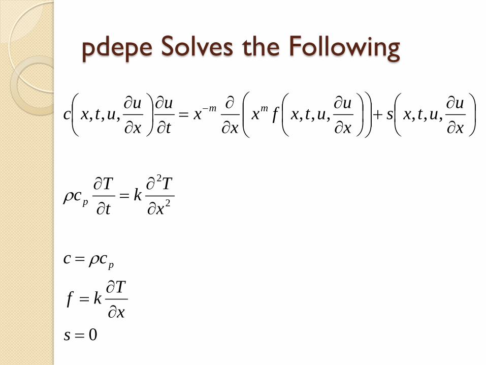
pdepe Solves the Following
0
,,,,,,,,,
2
2
s
x
Tkf
cc
x
Tk
t
Tc
x
uutxs
x
uutxfx
xx
t
u
x
uutxc
p
p
mm

Differential Equations
function [c,f,s] = pdex1pde(x,t,u,DuDx)
global rho cp k
c = rho*cp;
f = k*DuDx;
s = 0;
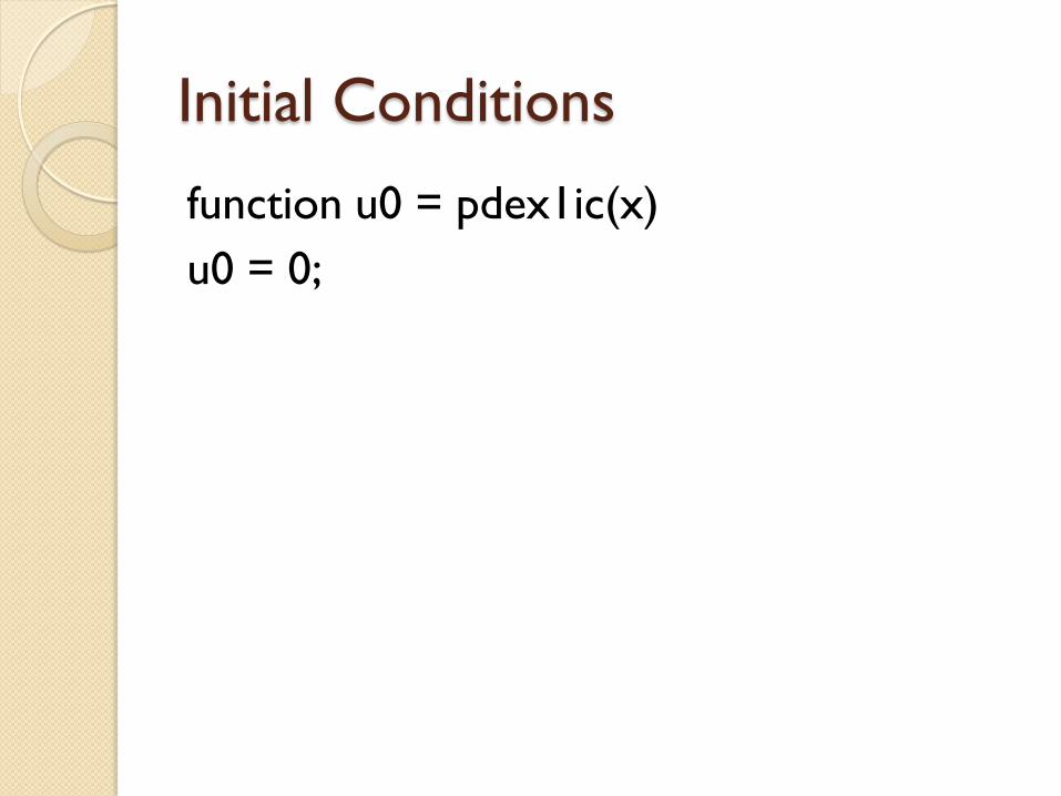
Initial Conditions
function u0 = pdex1ic(x)
u0 = 0;

pdepe Solves the Following
0,,,,,,
x
uutxftxqutxp
0),(
0''
''
0
0
tLT
x
Tkf
remember
x
Tkq
or
qx
Tk
x
x
0
q
urTp
Lx
1
''
0
q
qp
x
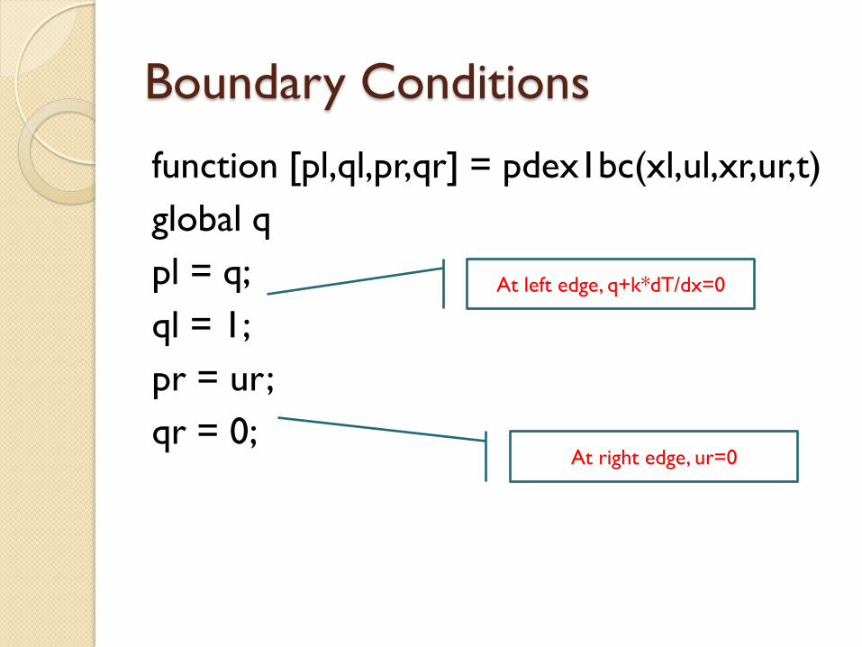
Boundary Conditions
function [pl,ql,pr,qr] = pdex1bc(xl,ul,xr,ur,t)
global q
pl = q;
ql = 1;
pr = ur;
qr = 0;At right edge, ur=0
At left edge, q+k*dT/dx=0

Calling the solver
tend=10
m = 0;
x = linspace(0,L,200);
t = linspace(0,tend,50);
sol =
pdepe(m,@pdex1pde,@pdex1ic,@pdex1bc,x,t);
200 spatial mesh points
50 time steps from t=0 to tend
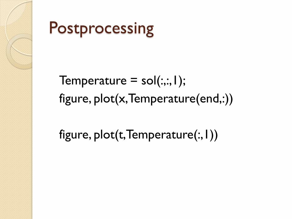
Postprocessing
Temperature = sol(:,:,1);
figure, plot(x,Temperature(end,:))
figure, plot(t,Temperature(:,1))

Full Code
function parabolic
global rho cp k
global q
L=0.1 %m
k=200 %W/m-K
rho=10000 %kg/m^3
cp=500 %J/kg-K
q=1e6 %W/m^2
tend=10 %seconds
m = 0;
x = linspace(0,L,200);
t = linspace(0,tend,50);
sol = pdepe(m,@pdex1pde,@pdex1ic,@pdex1bc,x,t);
Temperature = sol(:,:,1);
figure, plot(x,Temperature(end,:))
function [c,f,s] = pdex1pde(x,t,u,DuDx)
global rho cp k
c = rho*cp;
f = k*DuDx;
s = 0;
function u0 = pdex1ic(x)
u0 = 0;
function [pl,ql,pr,qr] = pdex1bc(xl,ul,xr,ur,t)
global q
pl = q;
ql = 1;
pr = ur;
qr = 0;

A Second Problem
Suppose we want convection at x=L
That is
0
dx
dTkhThT
or
TThdx
dTk
bulk
bulk
0,,,,,,
x
uutxftxqutxp
1
q
TurhTp
Lx
bulk

Altered Code
function u0 = pdex1ic(x)
global q hcoef Tbulk
u0 = Tbulk;
function [pl,ql,pr,qr] = pdex1bc(xl,ul,xr,ur,t)
global q hcoef Tbulk
pl = q;
ql = 1;
pr = hcoef*(ur-Tbulk);
qr = 1;

Download Scripts
http://blanchard.ep.wisc.edu/


