-- e R A Discontinuous Galerkin Method for Parabolic Problems with Modified hpFinite Element Approximat ion Technique Hideaki Kaneko* Department of Mathematics and Statistics Old Dominion University Norfolk, VirgiD-ia 23529-0077 Kim S. Bey Thermal Structures Branch Structure Division NASA Langley Research Center Hampton, VA 23681 Gene J. W. Hout Department of Mechanical Engineering Old Dominion University Norfolk, Virginia 23529 0 https://ntrs.nasa.gov/search.jsp?R=20040073488 2018-05-19T14:01:14+00:00Z
A Discontinuous Galerkin Met hod for Parabolic Problems
with Modified @Finite Approximation Technique
H. Kaneko, G. J. W. Hou, and K. S. Bey
Abstract
A recent paper [l] is generalized to a case where the spatial region is taken in @. The region is assumed to be a thin body, such as a panel on the wing or fuselage of
an aerospace vehicle. The traditional h- as well as hp-finite element methods are
applied to the surface defined in the z - y variables, while, through the thickness,
the technique of the p-element is employed. Time and spatial discretization scheme
developed in [l], based upon an assumption of certain weak singularity of IIutl12, is
used to derive an optimal a priori error estimate for the current method.
In this paper, the discontinuous Galerkin method is applied to the following standard
model problem of parabolic type:
Find u such that
where R is a closed and bounded set in R3 with boundary asZ, R+ = ( O , o o ) , Au =
a2u/ax2 + a2/ay2 + a2u/az2, ut = &/at, and the functions f and uo are given data.
'This author is supported by NASA- Grant NAG-1-01092
+This author is supported by NASA- Grant NAG-1-2300
1
The discontinuous Galerkin method is a robust finite element method that can deliver
high-order numerical approximation using unstructured grids. In this paper, region fl is
assumed to be a thin body in R3, such as a panel on the wing or fuselage of an aerospace
vehicle. The traditional h- as well as hp-finite element approximations are used in the
z - y variables, whereas, the p-finite element method developed, e.g., in [5],[15], is used
in the z variable which describes the region through the thickness. The application of the
p-finite element method through the thickness of thin structure, as compared to applying
the h- or hp-finite element discretization to all coordinate directions, enables us to
avoid structuring elements in P that are too thin to satisfy the required quasi-uniformity
condition (e.g. see [7]) that is necessary to deliver stable numerical approximation. We
are coining the term ‘modified hp’-finite element method, as it differs from the traditional
hp-finite element method which uses h- and p-finite elements on the same domain where
the h-finite e!emer?t umretthcd prcvides a refineme& ef the regic:: a ~ d t he p-Fiite e!eme;;t
provides an enrichment. In Section 2, approximation power of the modified hp-finite
element method will be investigated. In Section 3, the discontinuous Galerkin method
with the modified hpfinite element approximation technique is established. Discontinuity
is in time variable and time discretization is based upon the degree of singularity of 11.t1I2. The traditional h-finite element method is employed in time. The convergence analysis
given in [9] will be used. The reader is also reminded of recently published important
paper [16] by Schotzau and Schwab in which various time discretization techniques are
discussed. For instance, an exponential convergence rate in time of p-finite element
method is obtained in [16] despite the presence of singularity in the transient phase of
the solution. Time discretization used there is geometric. Schotzau and Schwab’s result
extends the results in [3] and [4] in which no exponential convergence rate is reported.
Also they discuss the h-finite element technique in time using a class of radical mesh and
obtain the algebraic convergence rate which is optimal. The radical mesh was chosen by
analyzing the incompatibility between initial and boundary data. The present authors [l]
established a similar time discretization technique for the discontinuous Galerkin finite
element method, h-version in time, which was based upon the singularity of 1 1 ~ ~ 1 1 ~ . Using
2
this analysis, it is shown in [l] that the optimal algebraic convergence rate in time of the
discontinuous Galerkin method can be obtained under more dispersed, therefore more
computationally stable radical mesh than the mesh used in [16].
2 Approximation Power of Modified hp Elements
Let w E. R2 and I' C R be convex regions. For simplicity, it is assumed that r = [-$, $1 where d = Irl. For simplicity, the thickness, d, is assumed constant over the domain. The
Sobolev space of order k defined on w x I' is denoted by Hk(w x I') with the norm
ll~112kwxr = c IID"~lG, o l l a l l k
where for each multi-integer a = (a1, a2, a3), we have let la1 = a1 + a2 + a3 and
We note that the Sobolev norm reduces to the usual LZ norm when k = 0. In this section,
a best possible error estimate is derived for approximating an element in Hk(w x I?) by
the finite element function spaces. Let Kt,q denote the master triangular element defined
Kc,,,={(<,q)€ R2: O I q I ( l + < ) & - 1 1 < 1 0 o r bY
O I q I ( 1 - J ) f i Oltll). Let SP(Kc,,) denote the space of polynomials of degree 1 p on Kc,,,, -i.e.,
SP(Kc,?) = span(c$: i,j = 0,1,. . . , p ; i + j 1 p } .
First, the shape functions for the master element KC,^ are formed. To accomplish this,
the barycentric coordinates are introduced via
Xi's form a partition of unity and X i is identically equal to one at a vertex of Kc,,, and
vanishes on the opposite side of KC,^. The hierarchical shape functions on Kt,? consists
3
I I
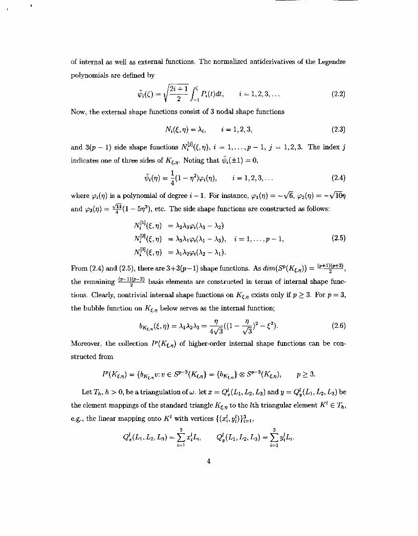
of internal as well as external functions. The normalized antiderivatives of the Legendre
polynomials are defined by
Now, the external shape functions consist of 3 nodal shape functions
N i ( t , 77) = Xi, i = 1,2 ,3 , (2.3)
and 3(p - 1) side shape functions Ni lil (t, q) , i = 1, . . . , p - 1, j = 1,2,3. The index j
indicates one of three sides of KC,,. Noting that &(H) = 0,
1 &(q) = qz)(pi(q), i = 1 , 2 , 3 , . . . (2.4)
where (pi(q) is a polynomial of degree i - 1. For instance, (p1(q) = -&, (pz (q ) = -6% and cp3(q) = e ( 1 - 5q2) , etc. The side shape functions are constructed as follows:
Ni"'(c, 7) = X 2 X 3 ( p i ( x 3 - A,)
Np1(c7q) = X 3 X I ( p i ( X 1 - A , ) ,
~ F l ( t 7 V ) = ~ l ~ z c ~ i ( ~ 2 - ~ 1 ) -
i = 1 , . . . , p - 1, (2.5)
From (2.4) and (2.5), there are 3+3(p-1) shape functions. As dirn(SP(K~,,)) = I P + l ) @ t 2 ) , the remaining basis elements are constructed in terms of internal shape func-
tions. Clearly, nontrivial internal shape functions on KC,q exists only if p 2 3. For p = 3,
the bubble function on KC,q below serves as the internal function;
Moreover, the collection IP(Kc,,) of higher-order internal shape functions can be con-
structed from
Let Th, h > 0, be a triangulation of w. let x = Qk(L1, L2, L3) and y = Qk(L1, Lz, L3) be
the element mappings of the standard triangle KC,^ to the Zth triangular element K' E T',
e.g., the linear mapping onto K' with vertices {(xf, Y : ) } ; = ~ , 3
4
The space of all polynomials of degree 5 p on K' is denoted by SP(Kz) and its basis can
be formed from the shape functions of Sp(Kc,,) described above by transforming them
under Qi and QL. The finite element space SP,'(w, Th) is now defined. For w , p 2 0 and
k 1 O? S p ' k ( ~ , T h ) = {U E Hk(w) : U I K E S P ( K ) , K E Th}. (2-7)
Assume that a triangulation {Th}, h > 0, of w consists of {KL}Ey' and that h' =
diam(K;), for I = I , . . . ,M(h) .
In the z-variable for through the thickness approximation, the local variable r is defined
in the reference element [-1,1] and I' is mapped onto the reference element by Qz, i.e.,
Clearly, QL is a linear function defined by
i d i d = & z ( ~ ) = -(I- T)(--) + -(I + T)S, 2 2 2 E [--I, 11
The Jacobian of Qz is constant dz - d dr 2'
In this paper, the basis functions of Pp([-l,1]) are taken to be the onedimensional
hierarchical shape functions. See [15] for a complete discussion of the basis elements used
in the p and hpfinite element methods.
_ - -
For example, in approximating an element in H'[-l, 11, with 1 = 0, Qi(7) = e-.l(~), 1 5 i 5 p + 1, where Pi-l is the Legendre polynomial of degree i - 1, form the hierarchical
basis functions. With 1 = 1, the external ($1 and Q2) and internal ($J~, i 2 3) shape
functions are defined by
Note that $i's form an orthogonal family with respect to the energy inner product (., -)E,
1 1
-1 -1 ($4, $ j ) E f J $i(t)$j(t)dt = 1 P,(t)P,(t)dt = 6ij.
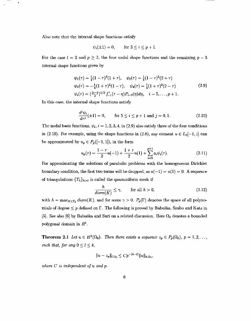
Also note that the internal shape functions satisfy
For the case 1 = 2 and p 1 3, the four nodal shape functions and the remaining p - 3
2i-5 112 T $ i ( T ) = ( T ) J - 1 ( ~ - q ) P i - 3 ( q ) d q , i = 5 ,..., p + l .
In this case, the internal shape functions satisfy
dj $i d r j -(H) = 0, for 5 5 i 5 p + 1 a n d j = 0, l . (2.10)
The nodal basis functions, $i , i = 1,2,3,4, in (2.9) also satisfy three of the four conditions
in (2.10). For example, using the shape functions in (2.8), any element u E L2[-i, ij can
be approximated by up E Pp([-1, l]), in the form
(2.11)
For approximating the solutions of parabolic problems with the homogeneous Dirichlet
boundary condition, the first two terms will be dropped, as u(-1) = u(1) = 0. A sequence
of triangulations {Th}h>O is called the quasiuniform mesh if
< y, for all h > 0, h
diam(K) - (2.12)
with h = maxKETh diarn(K), and for some y > 0. Pp(I') denotes the space of all polyno-
mials of degree 5 p defined on I'. The following is proved by Babu5ka, Szabo and Katz in
[5]. See also [SI by BabuSka and Suri on a related discussion. Here Ro denotes a bounded
polygonal domain in R2.
Theorem 2.1 Let u E Hk(s20). Then there exists a sequence zp E Pp(Ro), p = 1,2,. . . , such that, for any 0 5 1 5 I C ,
where C is independent of u and p .
6
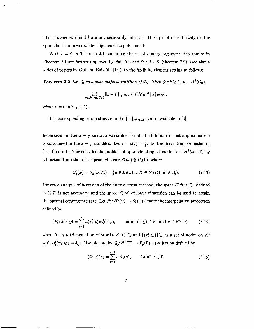
The parameters k and 1 are not necessarily integral. Their proof relies heavily on the
approximation power of the trigonometric polynomials.
With 1 = 0 in Theorem 2.1 and using the usual duality argument, the results in
Theorem 2.1 are further improved by Babugka and S u i in [6] (theorem 2.9), (see also a
series of papers by Gui and BabGka [13]), to the hpfinite element setting as follows:
Theorem 2.2 Let T h be a quasiunzfonn partition of Szo. Then for k 2 1, u E Hk(Ro),
where v = min(k,p+ 1).
The corresponding error estimate in the 11 . ( I H k ( ( R o ) is also available in [SI.
h-version in the z - y surface variabies: First, the h-finite eiement approximation
is considered in the z - y variables. Let z = s(7) = $T be the linear transformation of
[-1,1] onto I?. Now consider the problem of approximating a function u E Hk(w x r) by
a function from the tensor product space Si(w) 8 PP(r) , where
For error analysis of h-version of the finite element method, the space S p > k ( ~ , T h ) defined
in (2.7) is not necessary, and the space S;l(w) of lower dimension can be used to attain
the optimal convergence rate. Let Pi: H2(w) -+ S ~ ( W ) denote the interpolation projection
defined by
r " I (Piu)(z, y) = u(zi, yi)cpi(z, y), for all (z, y) E K' and u E H k ( w ) , (2.14)
i=l
where Th is a triangulation of w with K' E T h and { ( z f , y ~ ) } ~ = l is a set of nodes on K'
with cpf(zi, yi) = 6,. Also, denote by Qp: H k ( r ) -+ Pp(r) a projection defined by
P+l
i=l (Qpu)(z) = Ui'Pi(z), for all z E r, (2.15)
7
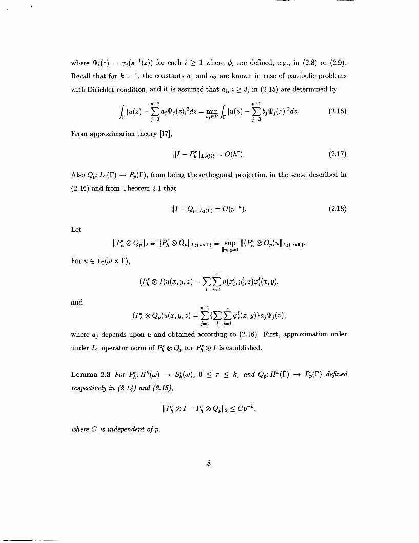
where ei(z) = Gi(s-l(z)) for each i 2 1 where qbi are defined, e.g., in (2.8) or (2.9).
Recall that for IC = 1, the constants a1 and a2 are known in case of parabolic problems
with Dirichlet condition, and it is assumed that ai, i 1 3, in (2.15) are determined by
From approximation theory [ 171,
111 - Ph'llLz(n) = O ( 0 (2.17)
Also Qp: L z ( ~ ) + PP(r), from being the orthogonal projection in the sense described in
(2.16) and from Theorem 2.1 that
Let
For u E L2(w x r),
and Ufl
where aj depends upon u and obtained according to (2.16). First, approximation order
under L2 operator norm of 5 @ Qp for @ I is established.
Lemma 2.3 For 5 : H k ( w ) -+ Si(w), 0 5 r 5 k, and QP:Hk(F) --t PP(r) defined
respectively in (2.14) and (2.15),
where C is independent of p.
8
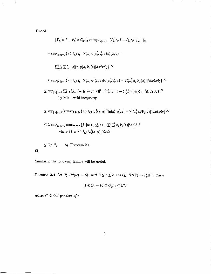
I Cp-&, by Theorem 2.1. 0
Similarly, the following lemma will be useful.
Lemma 2.4 Let q: H k ( u ) -+ Si , with 0 5 r 5 k and Qp: Hk(( r ) + Pp(r) . Then
111 @ Qp - Pi 8 I Ch'
where C is independent of r.
9
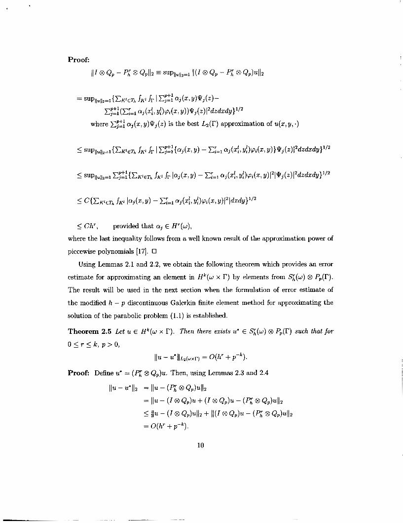
- < Ch', provided that aj f H'(w),
where the last inequality follows from a well known result of the approximation power of
piecewise polynomials [17]. 0
Using Lemmas 2.1 and 2.2, we obtain the following theorem which provides an error
estimate for approximating an element in H k ( u x r) by elements from Sl(w) @ Pp(I?).
The result will be used in the next section when the formulation of error estimate of
the modified h - p discontinuous Galerkin finite element method for approximating the
solution of the parabolic problem (1.1) is established.
10
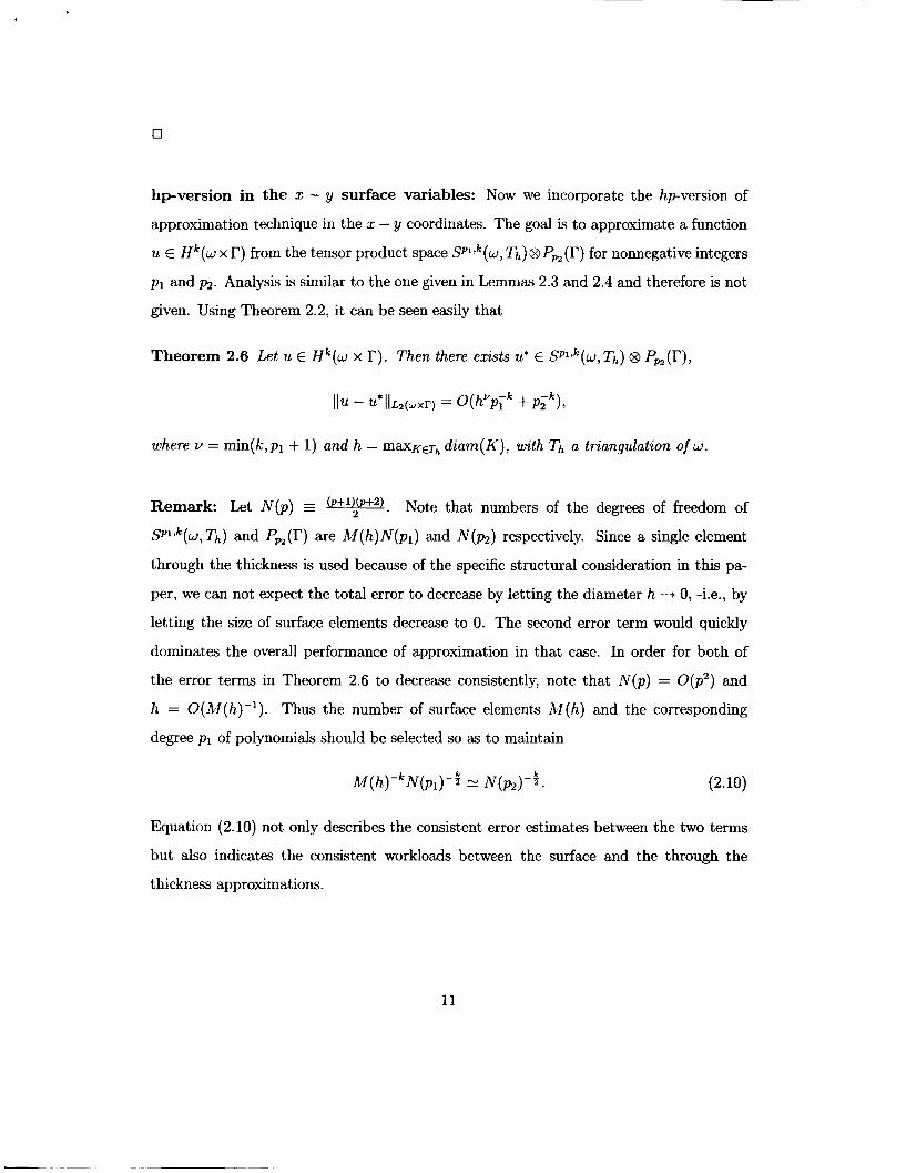
hpversion in the 2 - y surface variables: Now we incorporate the hpversion of
approximation technique in the z - y coordinates. The goal is to approximate a function
u E Hk(w x I?) from the tensor product space SP1tk(w, Th)@PP,(r) for nonnegative integers
pl and p z . Analysis is similar to the one given in Lemmas 2.3 and 2.4 and therefore is not
given. Using Theorem 2.2, it can be seen easily that
Theorem 2.6 Let u E H k ( u x r). Then there exists u* E Splik(w, Th) 8 Pm(I?),
where Y = min(k,pl + 1) and h = maxKeTh diam(K), with Th a triangulation of w.
Remark: Let N ( p ) v. Note that numbers of the degrees of freedom of
P l ~ ~ ( w , T h ) and Pp2(I') are M(h)N(pl) and N(pz ) respectively. Since a single element
through the thickness is used because of the specific structural consideration in this pa-
per, we can not expect the total error to decrease by letting the diameter h --+ 0, -i.e., by
letting the size of surface elements decrease to 0. The second error term would quickly
dominates the overall performance of approximation in that case. In order for both of
the error terms in Theorem 2.6 to decrease consistently, note that N ( p ) = O(J?) and
h = O(M(h)-'). Thus the number of surface elements M(h) and the corresponding
degree pl of polynomials should be selected so as to maintain
M(h) -kN(p l ) -$ N N ( p z ) - $ . (2.10)
Equation (2.10) not only describes the consistent error estimates between the two terms
but also indicates the consistent workloads between the surface and the through the
thickness approximations.
11
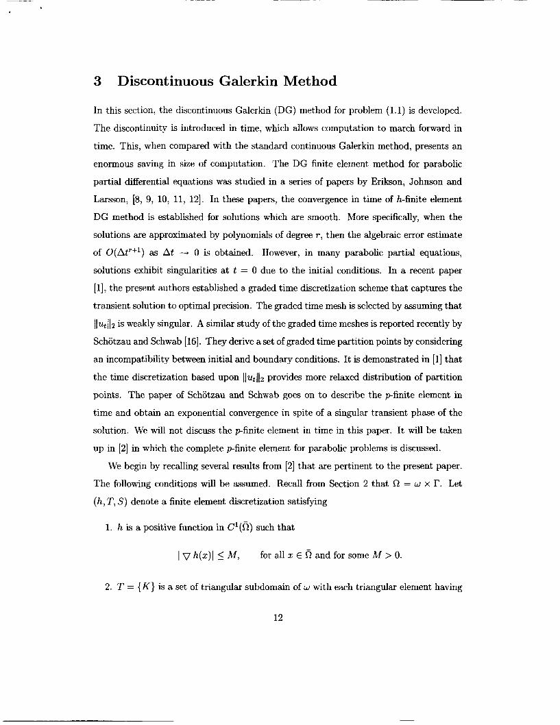
3 Discontinuous Galerkin Method
In this section, the discontinuous Galerkin (DG) method for problem (1.1) is developed.
The discontinuity is introduced in time, which allows computation to march forward in
time. This, when compared with the standard continuous Galerkin method, presents an
enormous saving in size of computation. The DG finite element method for parabolic
partial differential equations was studied in a series of papers by Erikson, Johnson and
Larsson, [8, 9, 10, 11, 121. In these papers, the convergence in time of h-finite element
DG method is established for solutions which are smooth. More specifically, when the
solutions are approximated by polynomials of degree T , then the algebraic error estimate
of O(AtT+') as At --+ 0 is obtained. However, in many parabolic partial equations,
solutions exhibit singularities at t = 0 due to the initial conditions. In a recent paper
[l], the present authors established a graded time discretization scheme that captures the
transient solution to optimal precision. The graded time mesh is selected by assuming that
llut112 is weakly singular. A similar study of the graded time meshes is reported recently by
Schotzau and Schwab [16]. They derive a set of graded time partition points by considering
an incompatibility between initial and boundary conditions. It is demonstrated in [l] that
the time discretization based upon 1 1 ~ ~ 1 1 ~ provides more relaxed distribution of partition
points. The paper of Schotzau and Schwab goes on to describe the pfmite element in
time and obtain an exponential convergence in spite of a singular transient phase of the
solution. We will not discuss the pfinite element in time in this paper. It will be taken
up in [2] in which the complete pfinite element for parabolic problems is discussed.
We begin by recalling several results from [2] that are pertinent to the present paper.
The following conditions will be assumed. Recall from Section 2 that R = w x r. Let
(h, T , S) denote a finite element discretization satisfying
1. h is a positive function in @(a) such that
I 7 h(z)l 5 M , for all z E !? and for some M > 0.
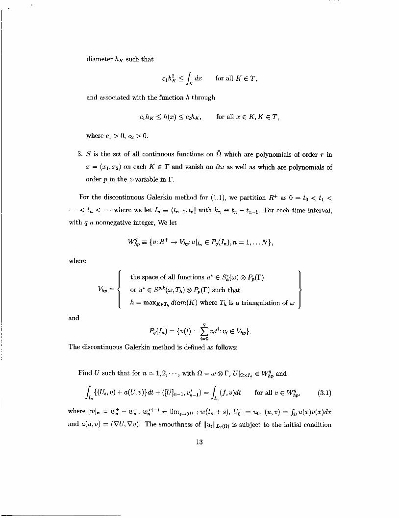
2. T = { K } is a set of triangular subdomain of w with each triangular element having
12
diameter hK such that
Clhi I J,.. for all K E T,
and associated with the function h through
clhK 5 h ( z ) 5 c2hK, for all z E K , K E T ,
where c1 > 0, c2 > 0.
3. S is the set of all continuous functions on fi which are polynomials of order r in
z = (zl, z 2 ) on each K E T and vanish on aw as well as which are polynomials of
order p in the z-variable in I'.
For the discontinuous Galerkin method for (l.l), we partition R+ as 0 = to < tl < (t,,-l.t,] with k? = tx - t,_:. For each time interval, ... < t , < ... where we let I,,
with q a nonnegative integer, We let
where
1 the space of all functions u* E S;l(w) 8 PP(r)
or u* E Splk(w,Th) 8 Pp(17) such that
h = maxKET,, diam(K) where T h is a triangulation of w
vhp =
P
Pq(I,) = {v(t) = vita: vi E VhP}. i=O
1 and
The discontinuous Galerkin method is defined as follows:
Find U such that for n = 1,2 , . . . , with R = w 8 r, U I o x ~ , E W;p and
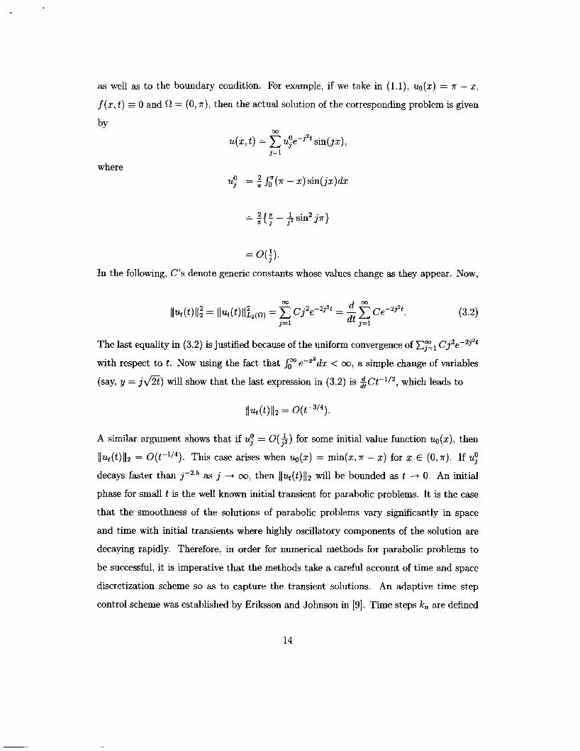
and a(u, u) = (VU, Vu). The smoothness of I lut l l~z(n, is subject to the initial condition
13
as well as to the boundary condition. For example, if we take in (l.l), uo(x) = T - z,
f(z, t ) E 0 and R = (0, T ) , then the actual solution of the corresponding problem is given
M 0 - j2t u(z, t ) = uje sin(jx),
j=l
where uj” = a J ~ ( T - x) sin(jz)dx
= O(j).
In the following, C’s denote generic constants whose values change as they appear. Now,
The last equality in (3.2) is justified because of the uniform convergence of cgl Cj2e-’jzt
with respect to t . Now using the fact that J ~ e - z z ~ < 00, a simple change of variables
(say, y = j&%) will show that the last expression in (3.2) is $Ct-1/2, which leads to
A similar argument shows that if uj” = O(f) for some initial value function uo(z), then
llut(t)ll2 = O(t-’l4). This case arises when ~ ( z ) = min(z, 7r - x) for z E (0, T). If uj”
decays faster than j-2.5 as j -+ 00, then I lq( t ) l l2 will be bounded as t -+ 0. An initial
phase for small t is the well known initial transient for parabolic problems. It is the case
that the smoothness of the solutions of parabolic problems vary significantly in space
and time with initial transients where highly oscillatory components of the solution are
decaying rapidly. Therefore, in order for numerical methods for parabolic problems to
be successful, it is imperative that the methods take a careful account of time and space
discretization scheme so as to capture the transient solutions. An adaptive time step
control scheme was established by Eriksson and Johnson in [9]. Time steps I C , are defined
14
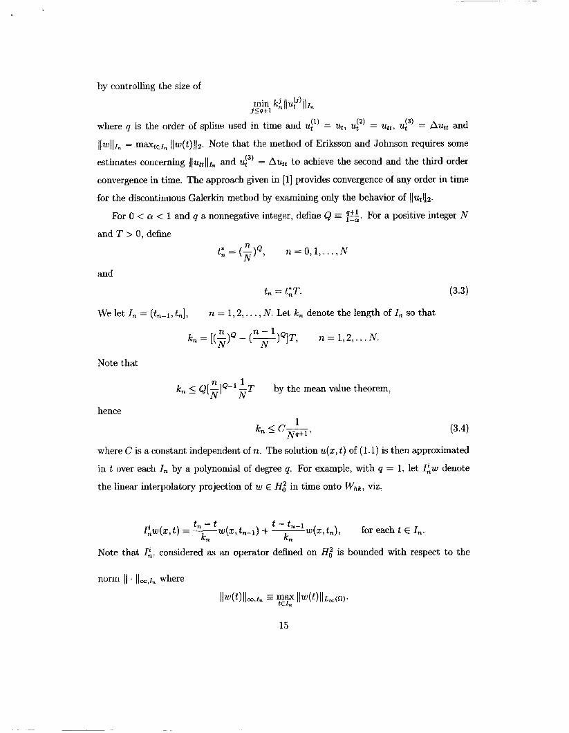
by controlling the size of . ci)
where q is the order of spline used in time and = ut, uj2) = uttr uj3) = Autt and
llwllr, = maxtEr, IJw(t)llz. Note that the method of Eriksson and Johnson requires some
estimates concerning Ilwllr, and up) = Aut, to achieve the second and the third order
convergence in time. The approach given in [l] provides convergence of any order in time
for the discontinuous Galerkin method by examining only the behavior of 11.t112.
min 4 I b t llr, j < q + l
For 0 < cr < 1 and q a nonnegative integer, define Q E. For a positive integer N
and T > 0, define n
“ N t* = ( - )Q , n = 0,1,. . . , N
and
t, = tET. (3.3)
We let I , = (4-1, t,], n = 1,2, . . . , N . Let k, denote the length of I , so that
n n - 1 kn = [(z)‘ - ( T ) ~ ] T , n = 1,2, . . . N .
Note that
n 1 N N
k, 5 Q[-IQ-’-T by the mean value theorem,
hence
(3.4) 1
kn I c-, Nq+’
where C is a constant independent of n. The solution u(z, t ) of (1.1) is then approximated
in t over each I , by a polynomial of degree q. For example, with q = 1, let I iw denote
the linear interpolatory projection of w E H i in time onto Whk, viz,
t , - t t - t,_’ IAw(s,t) = - ~ ( 5 , tn-1) + - w(z,tn), for each t E I,.
kn kn
Note that I:, considered as an operator defined on H i is bounded with respect to the
15
Since R is assumed to be of bounded domain, 1; is bounded with respect to 11 . 1 1 1 , also.
As was the case with the Lz projection, I: equals the identity on polynomials of degree
5 1. Expanding u(z, t ) in Taylor series with respect to t at t , to the first or to the second
order, we obtain, respectively, for each n = 1,2,. . . , N ,
(3.5)
Lemma 3.1 Let 0 < CY < 1, q a nonnegative integer and T > 0, we assume that tn,
n = 1,. . . , N am defined by (3.3). Then
where C, is a constant independent on N
Lemma 3.2 Let t, and I C , be defined by (3.3). Then
(1 lnm t R f l l 2 5 ."G, f67 ea& = (),I,. . . , 1 v . nT \ A I '"5
IC,
Lemma 3.2 is used to guarantee the stability of the discontinuous Galerkin method. In
the remainder of this paper, we illustrate the current 'modified ' hpfinite element method
by assuming the h-version in the surface z - y variables using the linear splines. Also
we illustrate the cases for constant as well as linear degree in time approximation. Let
{(xi, yi)}gl is the set of nodal points which are the interior vertices of K in Th. Let
'p j be the linear spline basis element defined by cpj(si, y i ) = S,, for i, j = 1, . . . M . The
superscript 1 used in (2.2) will be dropped. For application of higher order spline basis,
more nodal points are required over each K . The solution u of (1.1) is approximated by
(t > 0)
Note that u(zj, yj, re, 0), for j = 1,. . . , A4 are known from the initial condition. Also, for
t > 0, the boundary values u ( z j , y j , ~ $ , t ) are given. As u(3,t) = 0, for if E XI, t E R+
in ( l . l ) , (3.6) simplifies to
(3.7)
16
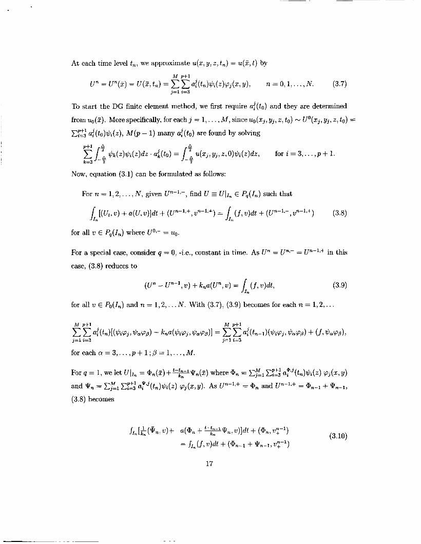
At each time level t,, we approximate u(5, y, z, tn) = u(3, t ) by
M p+l .
U" = ~ " ( 3 ) = U(z7 t n ) = C ai(tn)$i(z)pj(z, y), n = 0 ~ 1 , . . . N . (3.7) j=1 i=3
To start the DG finite element method, we first require uj(t0) and they are determined
from ~ ~ ( 3 ) . More specifically, for each j = 1 , . . . , M , since uo(q, yj, z , t o ) - U 0 ( q 7 yj, z, t o ) = P+l ai j (to)$i(z), M ( p - 1) many aj(to) are found by solving
Now, equation (3.1) can be formulated as follows:
For n = 1,2 , . . . , N , given Un-'t-, find U UII, E Pq(In) such that
l " [ ( U t 7 ZJ) + a(U, v)]dt + (un-l,+, vn-l,+) = J Ill ( j , w)dt + (U"+, v"-l,+) (3.8)
for all ZJ E P'(L,) where Uoi- = uo.
For a special case, consider q = 0, -i.e., constant in time. As U" = Uny- = Un-',+ in this
case, (3.8) reduces to
(U" - un- l , v) + k,a(Un, ZJ) = J ( j , ZJ)dt, (3.9) In
for all 21 E PO(1,) and n = 1 , 2 , . . . N . With (3.7), (3.9) becomes for each n = 1,2,. . .
For q = 1, we let U ~ I , = an(%)+ Y q n ( Z ) where a,, = p+l ai @,j (t,)$i(z) 'pj(z, y)
@, and Un-ly+ = @,-.I + @,-I7 and 9, = E:, CiZ3 ai ' (tn)$i(z) cpj(z, y). As Un-',+ =
(3.8) becomes
M
p+l @ j
17
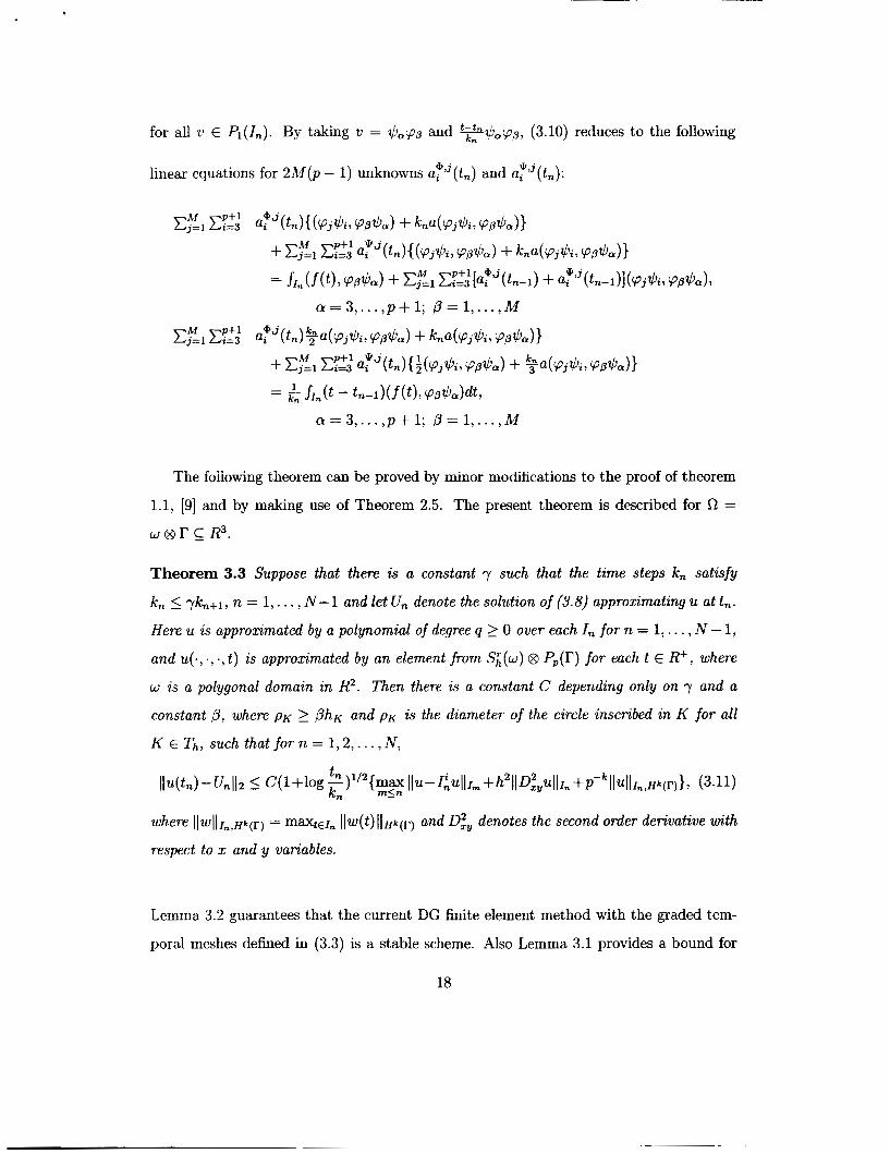
for all .u E PI(I,,). By taking .u = $,PO and Y ? , b n c p p , (3.10) reduces to the following
linear equations for 2M(p - 1) unknowns a:”(t,) and a”j(tn):
The foiiowing theorem can be proved by minor modifications to the proof of theorem
1.1, [9] and by making use of Theorem 2.5. The present theorem is described for S2 =
w @ r E R3.
Theorem 3.3 Suppose that there is a constant y such that the time steps kn satisfy
kn 5 yk,,+l, n = 1, . . . , N - 1 and let U,, denote the solution of (3.8) approximating u at t,.
Here u is approximated by a polynomial of degree q 2 0 over each In for n = 1 , . . . , N - 1,
and u(-, ., -, t ) is approximated by an element from SL(w) 18 PP(r) for each t E R+, where
w is a polygonal domain in R2. Then there is a constant C depending only on y and a
constant p, where p~ 2 P h K and p~ is the diameter of the circle inscribed in K for all
K E Th, such that for n = 1 , 2 , . . . , N ,
II~(tn)-unII2 I C(l+log -) tn 1/2 {mm I I u - I ~ u I I I , , , +h211~~,uIII,, +P-~IIuIII,, ,H~(~)), (3.11)
where IIZUllI,,,Hk(r) = maxtEI,, Ilw(t)llHk(p) and D& denotes the second order derivative with
respect to x and y variables.
k,, m<n
Lemma 3.2 guarantees that the current DG finite element method with the graded tem-
poral meshes defined in (3.3) is a stable scheme. Also Lemma 3.1 provides a bound for
18
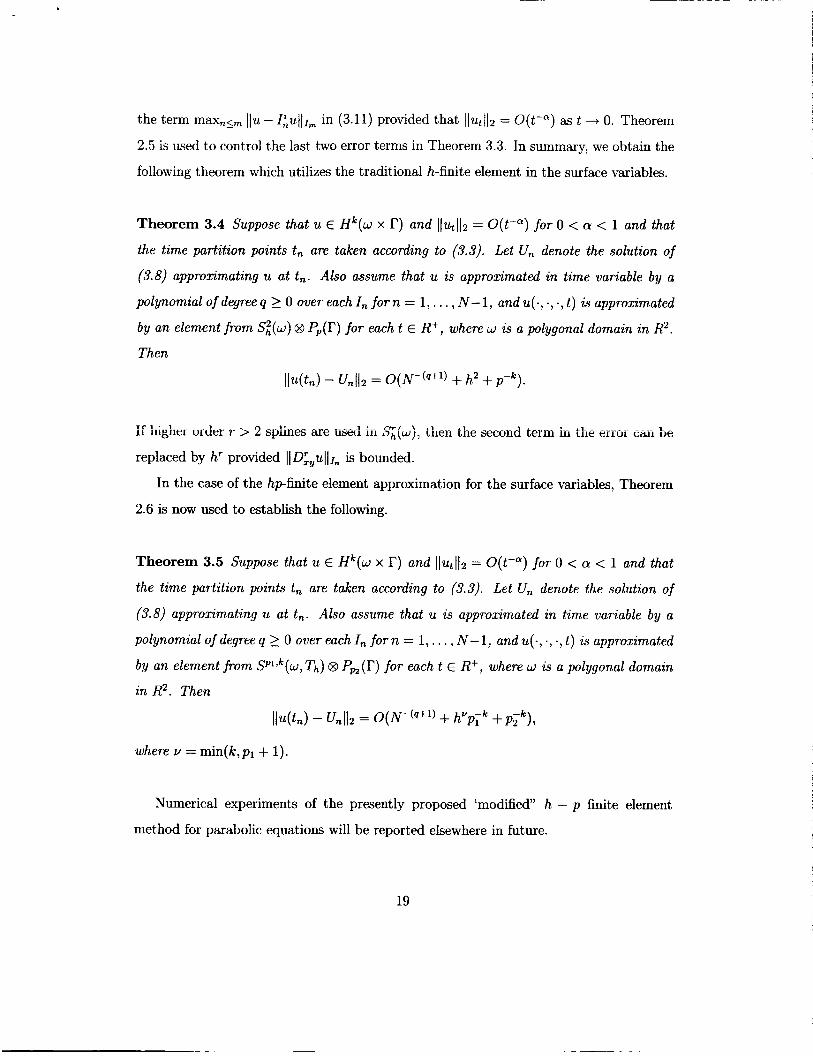
the term mu,<,,, IIu - I:ull~,,, in (3.11) provided that Ilutllz = O(t-") as t -+ 0. Theorem
2.5 is used to control the last two error terms in Theorem 3.3. In summary, we obtain the
following theorem which utilizes the traditional h-hi te element in the surface variables.
Theorem 3.4 Suppose that u f Hk(w x I?) and llut112 = O ( P ) for 0 < a < 1 and that
the time partition points t , are taken according to (3.3). Let U, denote the solution of
(3.8) approximating u at t,. Also assume that u is approximated in time variable by a
polynomial of degree q 2 0 over each I , for n = 1, . . . , N-1, and u(-, 0 , ., t ) is approximated
by an element from S;(w) @ PP(r) for each t E R+, where w is a polygonal domain in R2.
Then
IIu(t,) - U,ll2 = O(N-(q+') + hZ + P - ~ ) .
if ;&&er ~. > 2 SPliliW .&-e -u& iii tlleIi tiie secuiid teriii in tiie ei;loi c~~ be
replaced by h' provided IIDLYull~, is bounded.
In the case of the h p h i t e element approximation for the surface variables, Theorem
2.6 is now used to establish the following.
Theorem 3.5 Suppose that u E Hk(w x I?) and llq112 = O ( P ) for 0 < a < 1 and that
the time partition points t , are taken according to (3.3). Let U, denote the solution of
(3.8) approximating u at t,. Also assume that u is approximated in time variable by a
polynomial of degree q 2 0 over each I , for n = 1 , . . . , N-1, and u(-, ., 0 , t ) is approximated
by an element from Spl~~(w,Th) 8 PpL(I?) for each t E R+, where w is a polygonal domain
in Rz. Then
l I ~ ( t , ) - Unl12 = O(N-('+') + h"pYk +pyk ) ,
where v = min(lc,pl + 1).
Numerical experiments of the presently proposed 'modified" h - p finite element
method for parabolic equations will be reported elsewhere in future.
19
References
[l] Hideaki Kaneko, Kim S. Bey and Gene J. W. Hou,Discontinuous Galerkin finite
element method for parabolic problems, (preprint- Nov. 2000, NASA)
[2] Hideaki Kaneko and Kim S. Bey, Error analysis for p-version discontinuous Galerkin
method for heat transfer in built-up structuresjn preparation.
[3] I. BabuSka and T. Janik, The hp-version of the finite element method for parabolic
equations, I: The p-version in time,Numer. Methods P.D.E., Vol. 5, (1989), pp.
363-399.
[4] I. Babui3ka and T. Janik, The hp-version of the finite element method for parabolic
equations, II: The hp-version in tirne,Numer. Methods P.D.E., Vol. 6, (1990), pp.
343-369.
[5] I. Babwh, B. A. Szabo and I. N. Katz, The p-version of the finite element
method,SIAM J1. Num. Anal., Vol. 18, No.3, (1981), pp. 515-545.
[6] I. BabuSka and M. Suri, The p and hp versions of the finite element method, basic
principles and properties, SIAM Review, Vol. 36, No. 4, (1994), pp. 578-632.
[7] Claes Johnson, Numerical Solution of Partial Diflerential Equations by the Finite
Element Method,Cambridge University Press, (1994).
[8] Kenneth Eriksson and Claes Johnson, Error estimates and automatic time step
control for nonlinear parabolic problems, I, SIAM J1. Num. Anal., Vol. 24, No. 1,
(1987), pp.12-23.
[9] Kenneth Eriksson and C l m Johnson, Adaptive finite element methods for parabolic
problems I: a linear model problem, SIAM J1. Num. Anal., Vol. 28, No. 1, (1991),
pp. 43-77.
20
[lo] Kenneth Eriksson and Claes Johnson, Adaptive finite element methods for parabolic
problems II: Optimal error estimates in L,L2 and L,L,, SIAM J1. Num. Anal.,
Vol. 32, (1995), pp. 706-740.
[ll] Kenneth Eriksson and Clam Johnson, Adaptive finite element methods for parabolic