30
| Date post: | 31-Dec-2015 |
| Category: |
Documents |
| Upload: | laith-nunez |
| View: | 34 times |
| Download: | 1 times |

• PARAFAC is an N -linear model for an N-way array
• For an array X, it is defined as
denotes the array elements
are the model parameters
F is the number of fitted components
denotes the residuals
• The model parameters are typically grouped in N loading matrices
PARAFAC equation / 1
( )
1 2 1 211
N n N
F Nn
i i i i fi i inf
x a r==
= +å ÕK K
1 2 Ni i ix K
1 2 Ni i ir K
( )
n
ni fa
1 2 NI I I´ ´ ´K
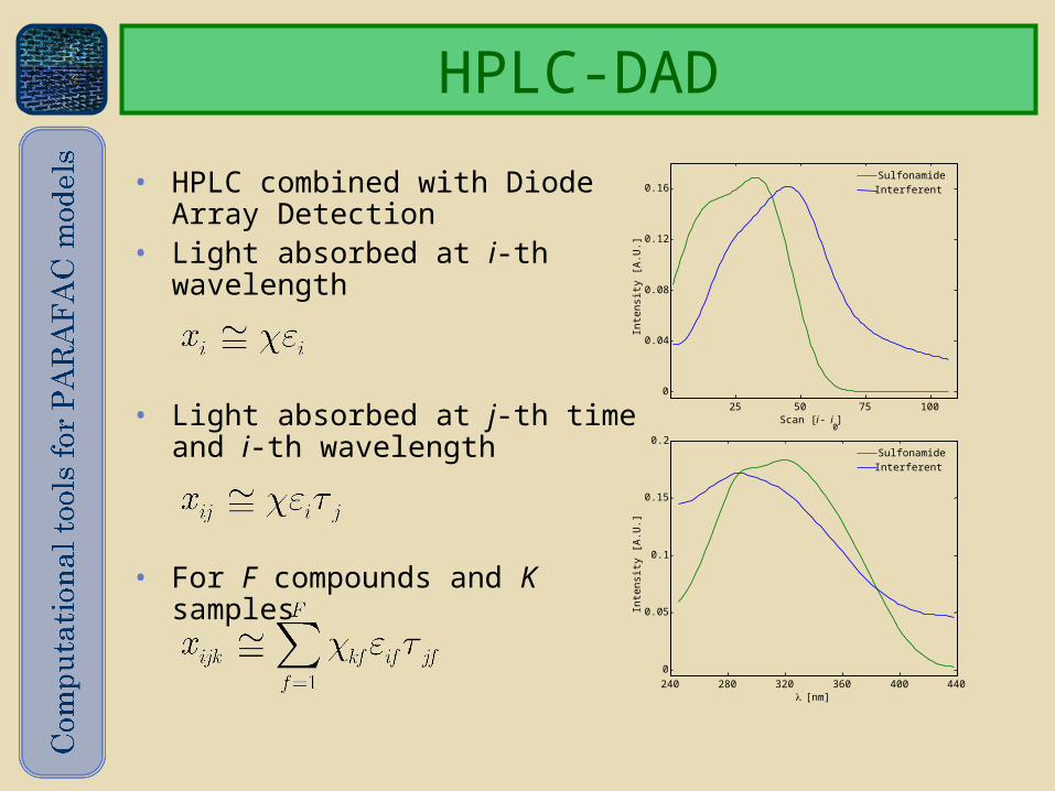
HPLC-DAD
• HPLC combined with Diode Array Detection
• Light absorbed at i-th wavelength
• Light absorbed at j-th time and i-th wavelength
• For F compounds and K samples
25 50 75 100
0
0.04
0.08
0.12
0.16
Scan [ i - i0]
Inte
nsi
ty [
A.U
.]
SulfonamideInterferent
240 280 320 360 400 440
0
0.05
0.1
0.15
0.2
[nm]
Inte
nsi
ty [
A.U
.]
SulfonamideInterferent
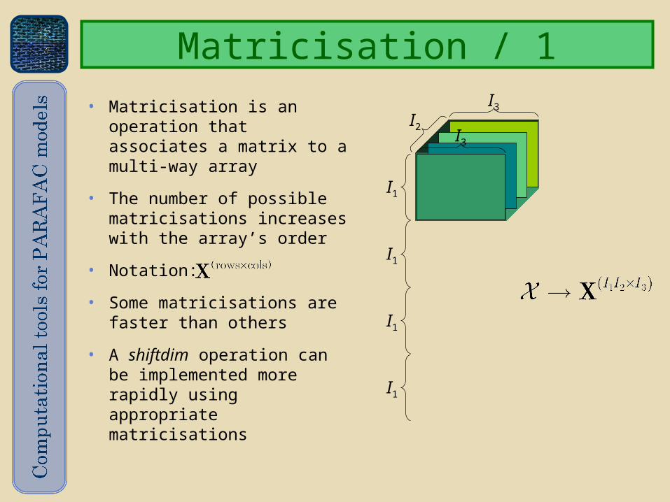
Matricisation / 1• Matricisation is an
operation that associates a matrix to a multi-way array
• The number of possible matricisations increases with the array’s order
• Notation:
• Some matricisations are faster than others
• A shiftdim operation can be implemented more rapidly using appropriate matricisations
I3I2
I1
I3
I1
I1
I1
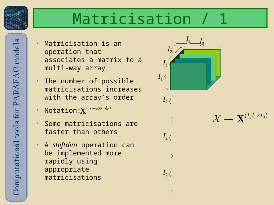
Matricisation / 1• Matricisation is an
operation that associates a matrix to a multi-way array
• The number of possible matricisations increases with the array’s order
• Notation:
• Some matricisations are faster than others
• A shiftdim operation can be implemented more rapidly using appropriate matricisations
I3I2
I1
I1
I2
I2
I2
I2

Vectorisation• The vec operator transforms a matrix in a vector
• In combination with matricisation one can define the vectorisation operation for N-way arrays
• The result of the vectorisation depends only the order of the modes in resulting from matricisation
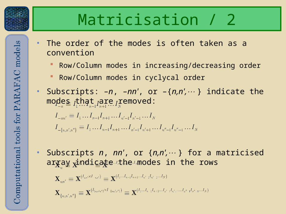
• The order of the modes is often taken as a convention Row/Column modes in increasing/decreasing order
Row/Column modes in cyclycal order
• Subscripts: –n, –nn', or –{n,n', } indicate the modes that are removed:
• Subscripts n, nn', or {n,n', } for a matricised array indicate the modes in the rows
Matricisation / 2
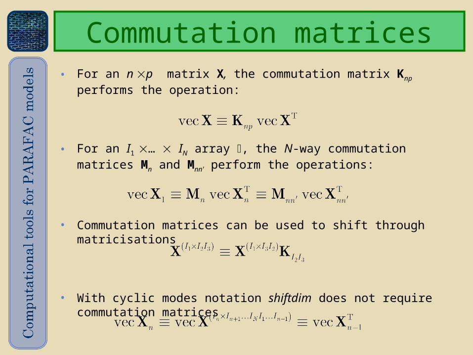
Commutation matrices• For an n p matrix X, the commutation matrix Knp performs
the operation:
• For an I1 … IN array , the N-way commutation matrices Mn and Mnn' perform the operations:
• Commutation matrices can be used to shift through matricisations
• With cyclic modes notation shiftdim does not require commutation matrices
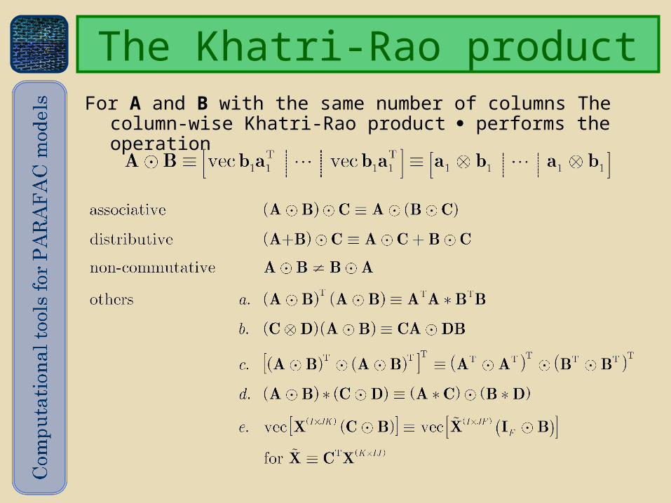
The Khatri-Rao productFor A and B with the same number of columns The column-
wise Khatri-Rao product performs the operation
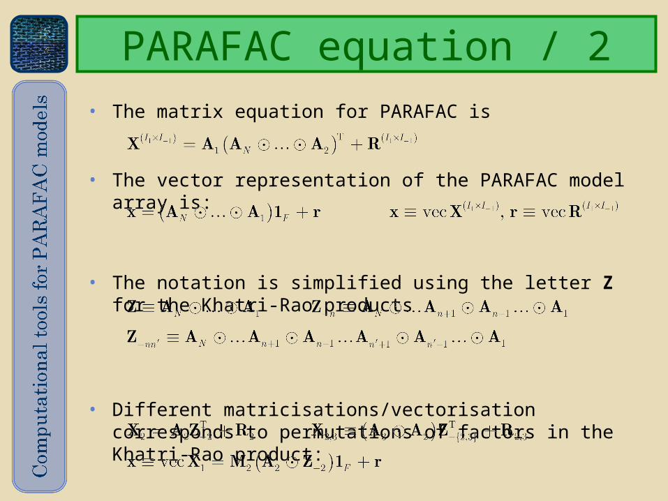
PARAFAC equation / 2• The matrix equation for PARAFAC is
• The vector representation of the PARAFAC model array is:
• The notation is simplified using the letter Z for the Khatri-Rao products
• Different matricisations/vectorisation corresponds to permutations of factors in the Khatri-Rao product:
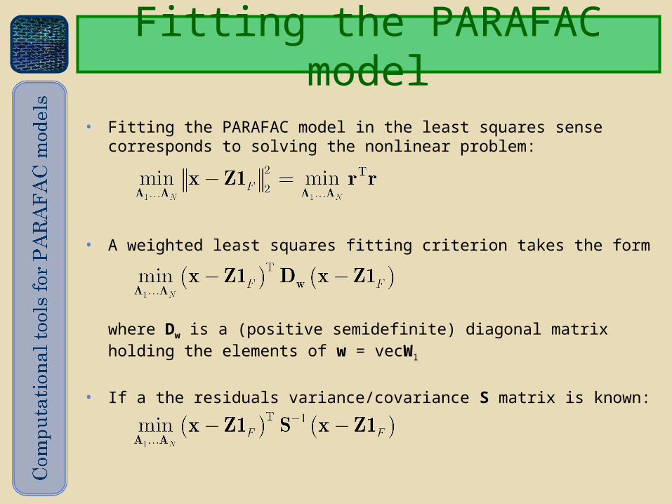
Fitting the PARAFAC model
• Fitting the PARAFAC model in the least squares sense corresponds to solving the nonlinear problem:
• A weighted least squares fitting criterion takes the form
where Dw is a (positive semidefinite) diagonal matrix holding the elements of w = vecW1
• If a the residuals variance/covariance S matrix is known:
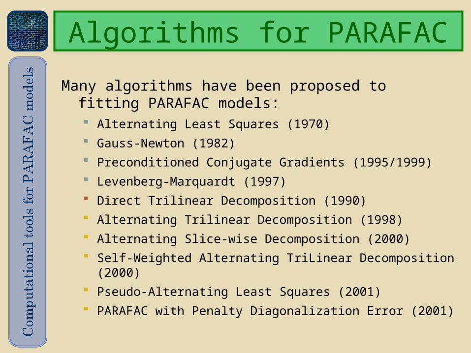
Algorithms for PARAFACMany algorithms have been proposed to fitting
PARAFAC models: Alternating Least Squares (1970) Gauss-Newton (1982) Preconditioned Conjugate Gradients (1995/1999) Levenberg-Marquardt (1997) Direct Trilinear Decomposition (1990) Alternating Trilinear Decomposition (1998) Alternating Slice-wise Decomposition (2000) Self-Weighted Alternating TriLinear Decomposition
(2000) Pseudo-Alternating Least Squares (2001) PARAFAC with Penalty Diagonalization Error (2001)

Alternating Least Squares
• ALS breaks down the nonlinear problem in linear ones, which are solved iteratively
Initial values for N-1 loading matrices must be provided
• The properties of the Moore-Penrose inverse and those of the Khatri-Rao product are used to reduce the computational load
• Convergence is checked at each step using (among others) the relative fit decrease
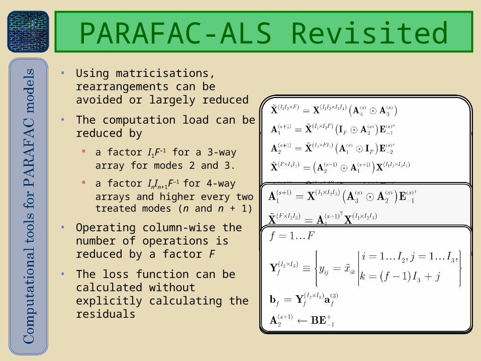
PARAFAC-ALS Revisited• Using matricisations,
rearrangements can be avoided or largely reduced
• The computation load can be reduced by
a factor I1F –1 for a 3-way
array for modes 2 and 3.
a factor InIn+1F –1 for 4-way
arrays and higher every two treated modes (n and n + 1)
• Operating column-wise the number of operations is reduced by a factor F
• The loss function can be calculated without explicitly calculating the residuals

• Line search extrapolation is used to accelerate convergence in ALS
• An analytical solution to the exact line search problem for PARAFAC
The optimal step length is found as the real root of a polynomial of degree 2N.
The cost for computing the polynomial coefficients directly is
• A great reduction in the number of iterations is obtained with simple and exact line search
Line search extrapolation
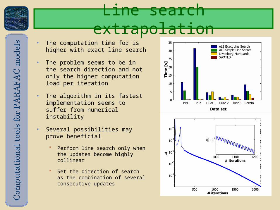
Line search extrapolation• The computation time for is
higher with exact line search
• The problem seems to be in the search direction and not only the higher computation load per iteration
• The algorithm in its fastest implementation seems to suffer from numerical instability
• Several possibilities may prove beneficial
Perform line search only when the updates become highly collinear
Set the direction of search as the combination of several consecutive updates
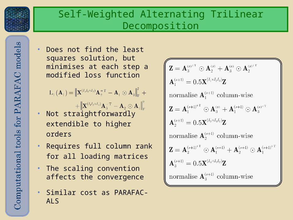
Self-Weighted Alternating TriLinear Decomposition
• Does not find the least squares solution, but minimises at each step a modified loss function
• Not straightforwardly extendible to higher orders
• Requires full column rank for all loading matrices
• The scaling convention affects the convergence
• Similar cost as PARAFAC-ALS

SWATLD
• SWATLD fitting criterion and convergence properties are not well characterised
• SWATLD yields biased loadings, which affects predictions
• SWATLD yields solutions with higher core consistency
• The results suggest that introducing such bias may be beneficial
• Naïve solutions (PARAFAC-PDE) lead to unstable algorithms
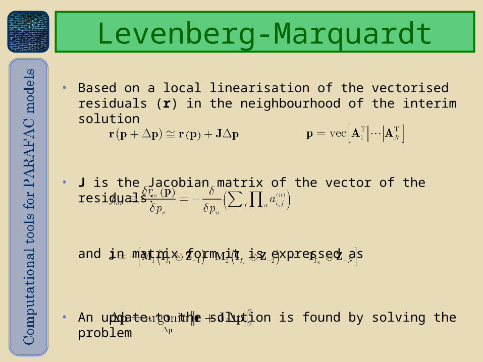
Levenberg-Marquardt
• Based on a local linearisation of the vectorised residuals (r) in the neighbourhood of the interim solution
• J is the Jacobian matrix of the vector of the residuals:
and in matrix form it is expressed as
• An update to the solution is found by solving the problem
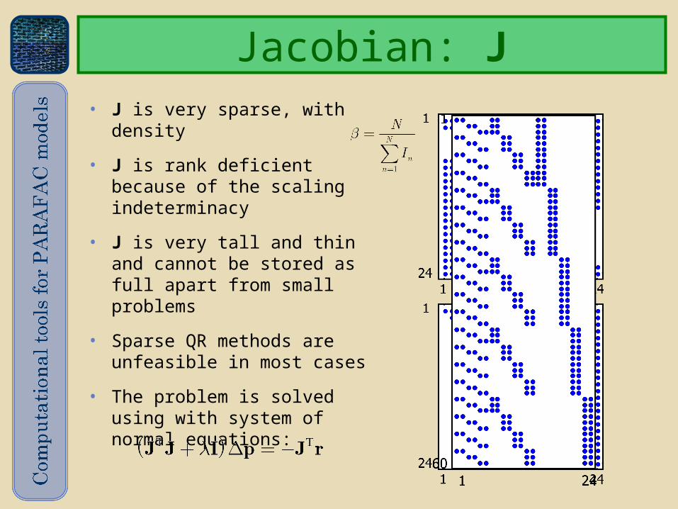
• J is very sparse, with density
• J is rank deficient because of the scaling indeterminacy
• J is very tall and thin and cannot be stored as full apart from small problems
• Sparse QR methods are unfeasible in most cases
• The problem is solved using with system of normal equations:
Jacobian: J

JTJ and JTDwJ• Both can be calculated
without forming J
• WLS case is much more expensive because of the calculation of U and V
• Time expense can be reduced using property e. and c. of the Khatri-Rao product
• Filling the sparse J and compute JTJ explicitly is faster for some WLS problems
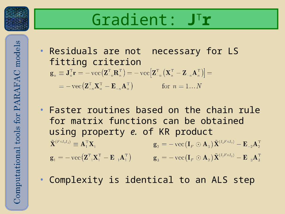
Gradient: JTr
• Residuals are not necessary for LS fitting criterion
• Faster routines based on the chain rule for matrix functions can be obtained using property e. of KR product
• Complexity is identical to an ALS step
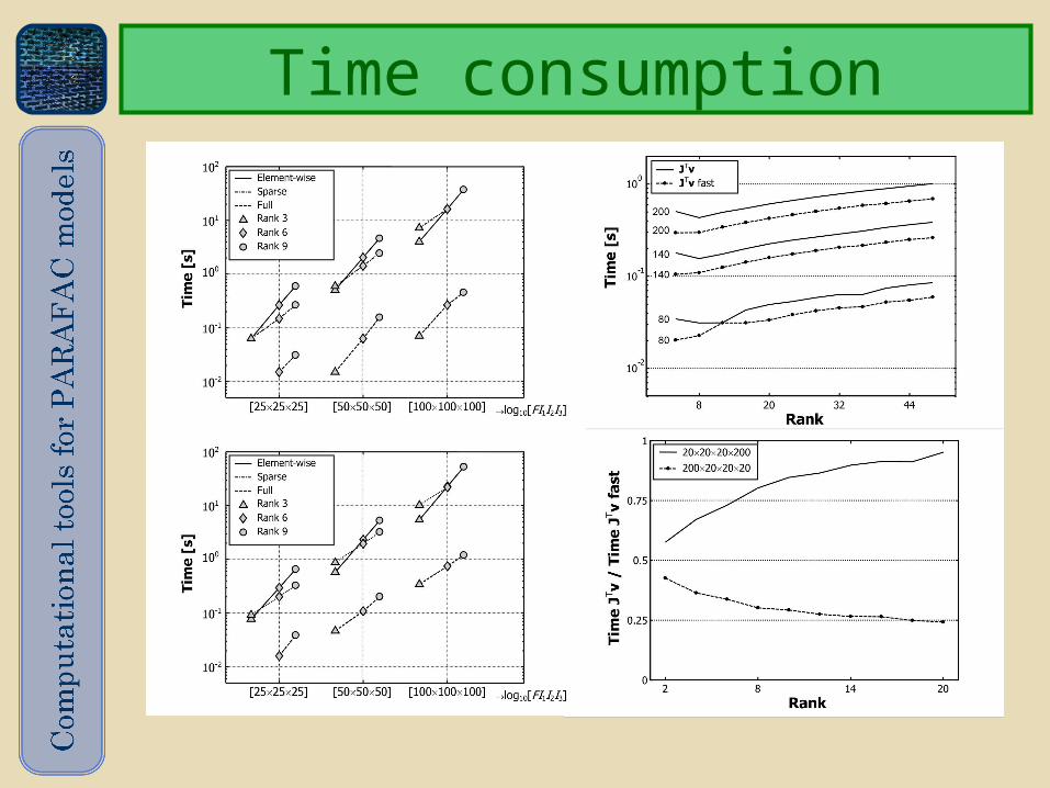
Time consumption
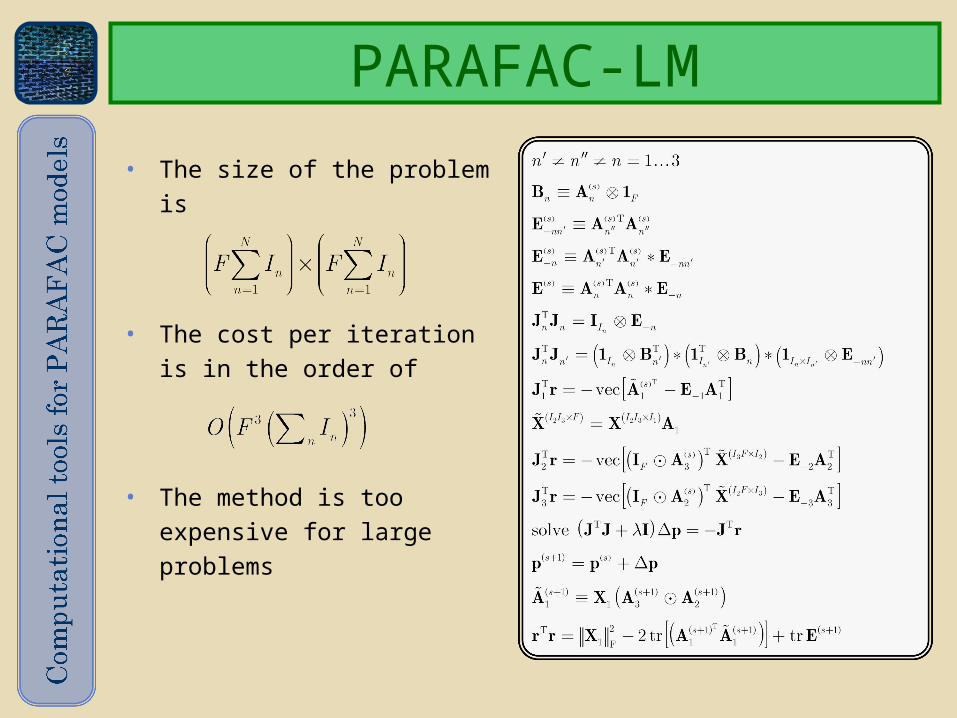
PARAFAC-LM
• The size of the problem is
• The cost per iteration is in the order of
• The method is too expensive for large problems
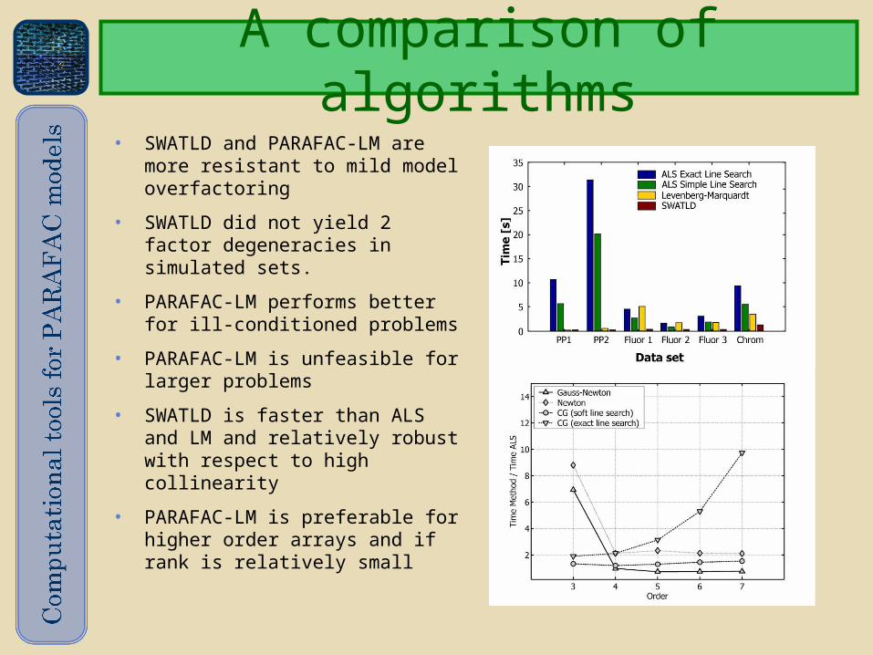
A comparison of algorithms
• SWATLD and PARAFAC-LM are more resistant to mild model overfactoring
• SWATLD did not yield 2 factor degeneracies in simulated sets.
• PARAFAC-LM performs better for ill-conditioned problems
• PARAFAC-LM is unfeasible for larger problems
• SWATLD is faster than ALS and LM and relatively robust with respect to high collinearity
• PARAFAC-LM is preferable for higher order arrays and if rank is relatively small
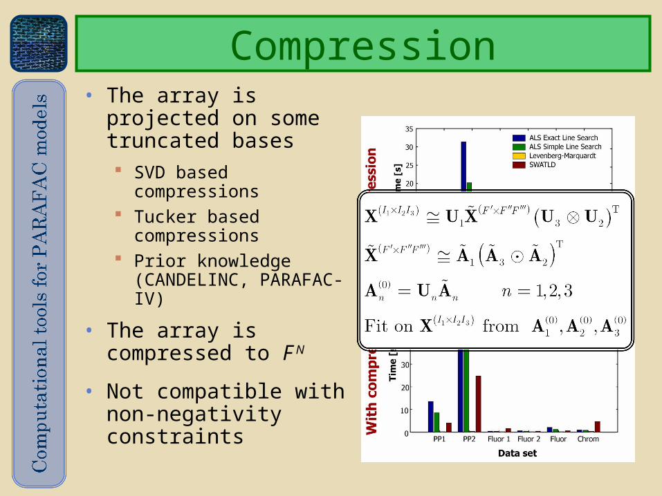
• The array is projected on some truncated bases SVD based
compressions Tucker based
compressions Prior knowledge
(CANDELINC, PARAFAC-IV)
• The array is compressed to F N
• Not compatible with non-negativity constraints
Compression
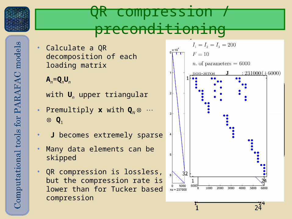
QR compression / preconditioning
• Calculate a QR decomposition of each loading matrix
An=QnUn
with Un upper triangular
• Premultiply x withQN Q1
• J becomes extremely sparse
• Many data elements can be skipped
• QR compression is lossless, but the compression rate is lower than for Tucker based compression
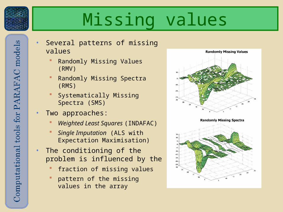
• Several patterns of missing values Randomly Missing Values (RMV) Randomly Missing Spectra (RMS) Systematically Missing Spectra
(SMS)
• Two approaches: Weighted Least Squares
(INDAFAC) Single Imputation (ALS with
Expectation Maximisation)
• The conditioning of the problem is influenced by the fraction of missing values pattern of the missing values in
the array
Missing values
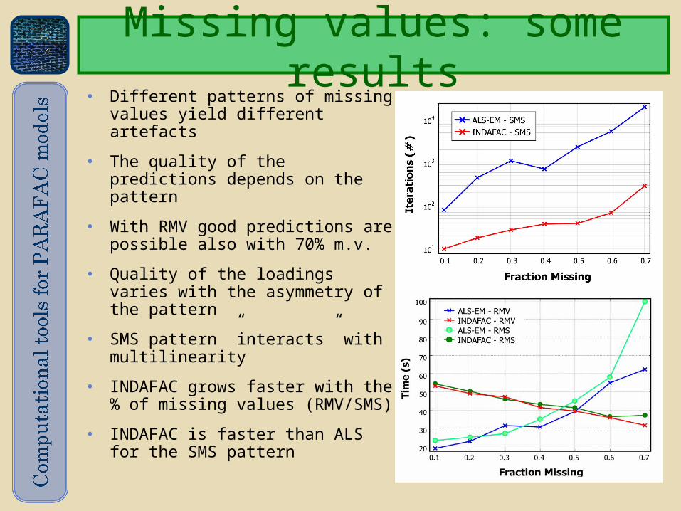
Missing values: some results
• Different patterns of missing values yield different artefacts
• The quality of the predictions depends on the pattern
• With RMV good predictions are possible also with 70% m.v.
• Quality of the loadings varies with the asymmetry of the pattern
• SMS pattern ”interacts” with multilinearity
• INDAFAC grows faster with the % of missing values (RMV/SMS)
• INDAFAC is faster than ALS for the SMS pattern
30
Final remarks• There appears to be no method superior to any
other in all conditions
• There is great need for numerical insight in the
algorithms. Faster algorithms may entail numerical
instability
• Several properties of the column-wise Khatri-Rao
product can be used to reduce the computation
load
• Numerous methods have not been investigated yet


![Equation Page Side 1[2]](https://static.documents.pub/doc/80x56/546507c6b4af9f0a328b46b5/equation-page-side-12.jpg)


