Parallel Algorithms for Fluid and Rigid Body Interaction Crist´ obal Samaniego Alvarado Advisor: Guillaume Houzeaux Co-advisor: Mariano V´ azquez Thesis submitted for the degree of Doctor of Philosophy Universitat Polit` ecnica de Catalunya Barcelona, Espa˜ na November 2015
Transcript
Parallel Algorithms for
Fluid and Rigid Body Interaction
Cristobal Samaniego Alvarado
Advisor: Guillaume Houzeaux
Co-advisor: Mariano Vazquez
Thesis submitted for the degree of Doctor of Philosophy
Universitat Politecnica de Catalunya
Barcelona, Espana
November 2015
Acknowledgements
As a personal matter, I prefer to write the acknowledgements in Spanish, mymother tongue.
Quiero empezar por agradecer a mi director de tesis, a Guillaume Houzeaux.Soy muy afortunado al haberle tenido como director. No solo por que es unapersona inteligente sino tambien amable y que disfruta de su trabajo. Graciaspor tu paciencia y dedicacion.
Tambien quiero agradecer al BSC (Barcelona Supercomputing Center), aldepartamento del CASE, por haber confiado en mi trabajo. Especialmente aMariano Vazquez. Fue el quien me conocio primero y en Ecuador. El vio quepodıa ayudarles de alguna manera y confio en mı. Nunca lo olvidare.
A mis companeros de trabajo y de oficina. Ninguno de ellos, me ha negadojamas ayuda.
A Paola, mi companera de viaje y de vida. Sin ella, todo esto hubiera sidomucho menos agradable. Se que todos los logros que he hecho, ella los ha hechosuyos. Me halaga que se sienta tan orgullosa de mı, es una de las razonesque mas me ha empujado a terminar este trabajo. Yo tambien me siento muyorgullaso de todo lo que ha logrado y esta a punto de lograr. Espero que esto aella tamien le sirva como me ha servido a mı.
A mi familia, a mis padres y hermanos. Ellos me llevaron hasta aquı. Meapoyaron y me siguieron como si fueran ellos los que estuvieran haciendo estetrabajo. A ellos es a los que mas extrano ahora que estamos en diferenrtes paısesy continentes. Esteban, ademas, estuvo conmigo ayudandome en mi tesis y mispublicaciones sin importar el dıa, la fecha o la hora. Sabıa que podıa contarcon el siempre. Se que Augusto, Haydee o Pedro hubieran hecho lo mismo si sucampo de trabajo hubiera sido parecido al mıo.
A mis amigos, a los que se fueron ya. Con Natalia, Juan Carlos y Oscarpasamos muy buenos tiempos en Barcelona. A los amigos de aca, de Cataluna.Ellos me han tratado como uno mas. Gracias Cristina, Laia, Jordi e Ivan.El dıa que me vaya, voy a extranar mucho las noches de comida, bebida, deconversaciones, de muy buenas conversaciones.
Summary
This thesis is based on the implementation of a computational system to nu-merically simulate the interaction between a fluid and an arbitrary numberof rigid bodies. This implementation was performed in a distributed memoryparallelization context, which makes the process and its description especiallychallenging. As a consequence, for the sake of descriptive precision and concep-tual clarity, a new formal framework using set theory concepts is developed.
The fluid is discretized using a non body-conforming mesh and the bound-aries of the bodies are embedded in this mesh. The force that the fluid exertson a body is determined from the residual of the momentum equations. Con-versely, the velocity of the body is imposed as a boundary condition in the fluid.In this context, two new approaches are proposed.
To account for the fact that fluid nodes can become solid nodes and vice versadue to the rigid body movement, we have adopted the FMALE approach, whichis based on the idea of a virtual movement of the fluid mesh at each time step.A new method of interpolation is adopted inside the FMALE implementationin order to improve the results.
The physics of the fluid is described by the incompressible Navier-Stokesequations. These equations are stabilized using a variational multiscale finiteelement method and solved using a fractional step like scheme at the algebraiclevel. The incompressible Navier-Stokes solver is a parallel solver based onmaster-worker strategy.
The bodies can have arbitrary shapes and their motions are determinedby the Newton-Euler equations. The contacts between bodies are solved us-ing impulses to avoid interpenetrations. The time of impact is determinedimplementing a dynamic collision detection algorithm. As far as the parallelimplementation is concerned, the data of all the bodies are shared by all thesubdomains. To track the boundary of the bodies in the fluid mesh, computa-tional geometry tools have been used.
List of publications
• C. Samaniego, G. Houzeaux, E. Samaniego, M. Vazquez, Parallel embed-ded boundary methods for fluid and rigid-body interaction, ComputerMethods in Applied Mechanics and Engineering 290 (2015) 387–419
• E. Casoni, A. Jerusalem, C. Samaniego, B. Eguzkitza, P. Lafortune, D. Tjah-janto, X. Saez, G. Houzeaux, M. Vazquez, Alya: computational solid me-chanics for supercomputers, Archives of Computational Methods in Engi-neering (2014) 1–20
• H. Owen, G. Houzeaux, C. Samaniego, A. Lesage, M. Vazquez, Recentship hydrodynamics developments in the parallel two-fluid flow solver alya,Computers & Fluids 80 (2013) 168–177
• G. Houzeaux, H. Owen, B. Eguzkitza, C. Samaniego, R. de la Cruz, H. Cal-met, M. Vazquez, M. Avila, Developments in Parallel, Distributed, Gridand Cloud Computing for Engineering, Vol. volume 31 of ComputationalScience, Engineering and Technology Series, Saxe-Coburg Publications,2013, Ch. Chapter 8: A Parallel Incompressible Navier-Stokes Solver: Im-plementation Issues, pp. 171–201
• H. Owen, G. Houzeaux, C. Samaniego, F. Cucchietti, G. Marin, C. Tripi-ana, H. Calmet, M. Vazquez, Two fluids level set: High performance sim-ulation and post processing, in: 2012 SC Companion: High PerformanceComputing, Networking, Storage and Analysis (SCC), IEEE, Salt PalaceConvention Center, Salt Lake City, UT, 2012, pp. 1559–1568
• G. Houzeaux, C. Samaniego, H. Calmet, R. Aubry, M. Vazquez, P. Rem,Simulation of magnetic fluid applied to plastic sorting, The Open WasteManagement Journal 3 (2010) 127–138
7.3 Fluid and rigid bodies interaction (collisions) . . . . . . . . . . . 967.3.1 Drafting, kissing and tumbling for two interacting spheres 987.3.2 Drafting, kissing and tumbling for more than two inter-
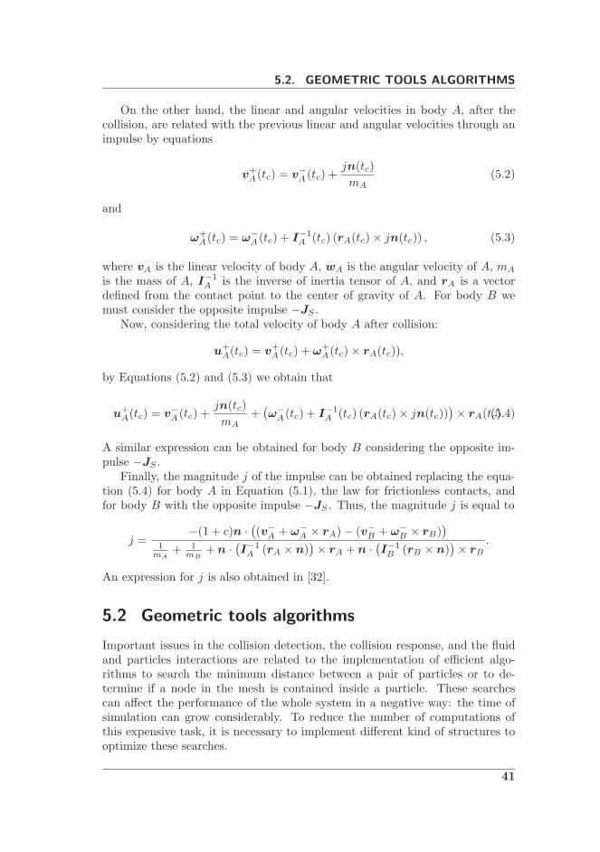
5.1 Missing collision. . . . . . . . . . . . . . . . . . . . . . . . . . . . 385.2 Closest points between the bodies A and B. . . . . . . . . . . . . 395.3 Contact between two bodies. . . . . . . . . . . . . . . . . . . . . 405.4 The skd-tree construction for a particle. The surface mesh of the
body has 8 edges. . . . . . . . . . . . . . . . . . . . . . . . . . . . 435.5 Bucket sort structure. In order to find the nodes inside the body,
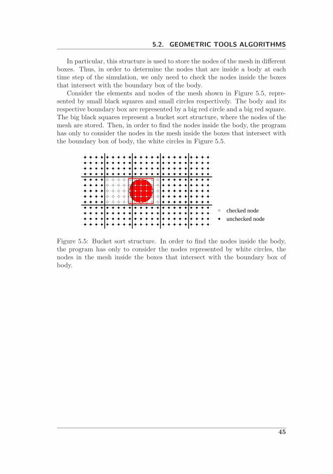
the program has only to consider the nodes represented by whitecircles, the nodes in the mesh inside the boxes that intersect withthe boundary box of body. . . . . . . . . . . . . . . . . . . . . . . 45
6.1 Hole elements and ΓS,h schematization. . . . . . . . . . . . . . . 486.2 Fringe, free and holes nodes. . . . . . . . . . . . . . . . . . . . . . 486.3 Near and inside nodes. . . . . . . . . . . . . . . . . . . . . . . . . 506.4 Array of data related with the set of nodes of S. The gray zone
represents the nodes take into account by S. . . . . . . . . . . . . 516.5 Sets of free nodes at different levels. The red concentric circles
6.6 A scheme of the algorithm that defines the movement of nodes.The body surface mesh is represented as ΓS,h. The parameterspfri and pfre are the proportions of the movement of the set offringe and free nodes respectively. And the value c is the centroiddefined by the set of nodes Cnod(n). . . . . . . . . . . . . . . . . . 56
6.7 The movement of a fringe node n considering only one increment.(Middle) First, we have to determine the centroid c of the setof nodes Cnod(n) ∩ Nfri. (Bottom) Then, we move the node ntowards the projection p of c on the boundary mesh. . . . . . . . 57
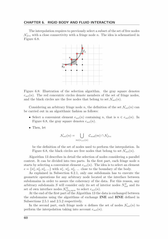
6.8 Illustration of the selection algorithm. the gray square denotesesel(n). The red concentric circles denote members of the set offringe nodes, and the black circles are the free nodes that belongto set Nsel(n). . . . . . . . . . . . . . . . . . . . . . . . . . . . . 60
6.9 Illustration of the FMALE framework. The dotted lines repre-sent the body surface mesh at the previous time step tn and thecontinuous lines represent the body surface mesh at the currenttime step tn+1. The red concentric circles denote members of theset of fringe nodes, black circles members of the set of free nodes,and crosses members of the set of hole nodes. The plots (a) and(c) represent the fluid mesh in two consecutive time steps afterremeshing. . . . . . . . . . . . . . . . . . . . . . . . . . . . . . . . 64
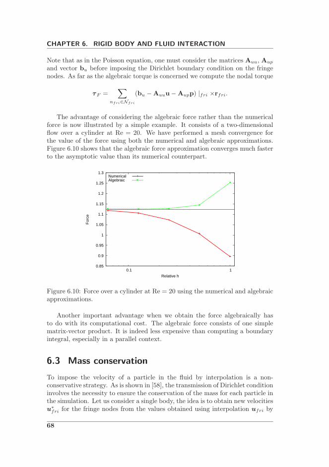
6.10 Force over a cylinder at Re = 20 using the numerical and alge-braic approximations. . . . . . . . . . . . . . . . . . . . . . . . . 68
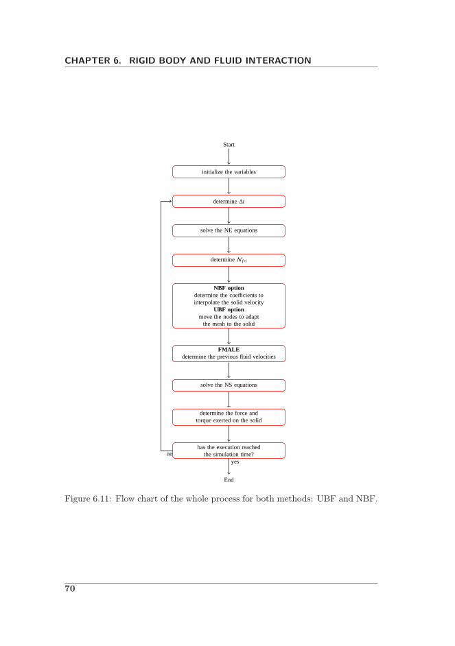
6.11 Flow chart of the whole process for both methods: UBF and NBF. 70
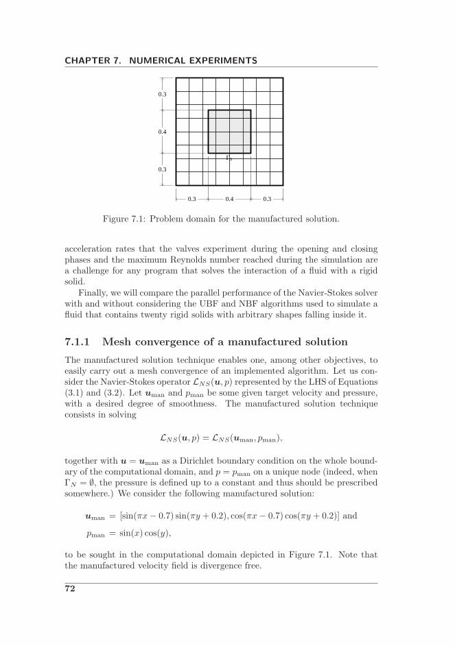
7.1 Problem domain for the manufactured solution. . . . . . . . . . . 72
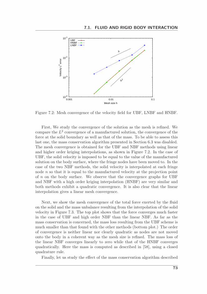
7.2 Mesh convergence of the velocity field for UBF, LNBF and HNBF. 73
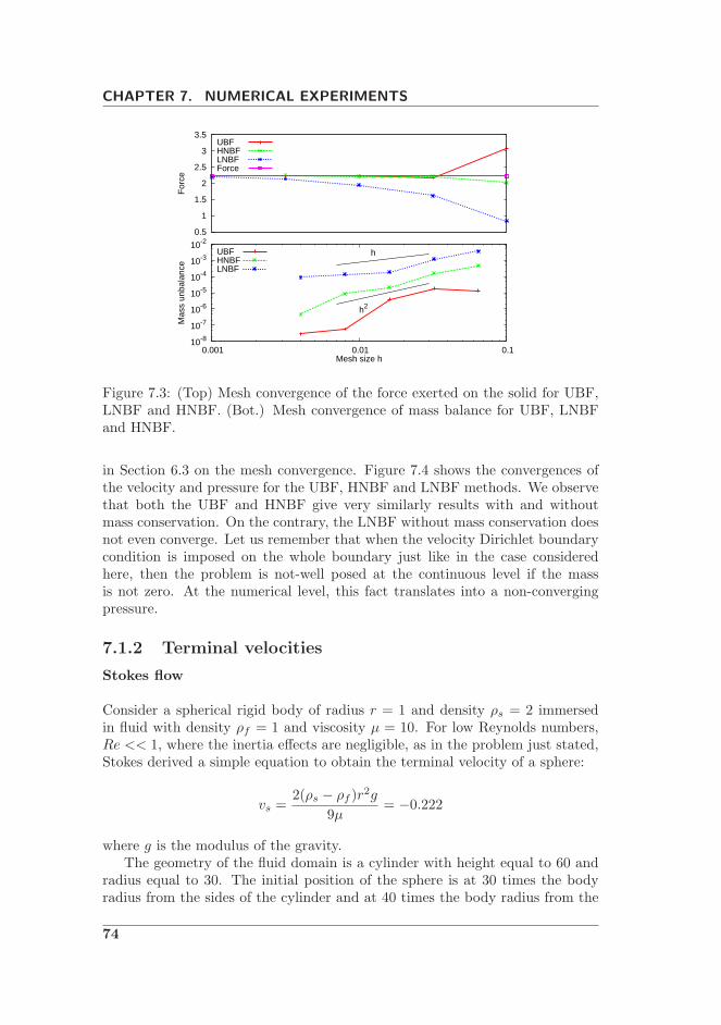
7.3 (Top) Mesh convergence of the force exerted on the solid for UBF,LNBF and HNBF. (Bot.) Mesh convergence of mass balance forUBF, LNBF and HNBF. . . . . . . . . . . . . . . . . . . . . . . . 74
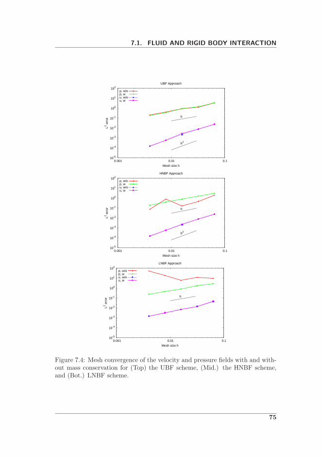
7.4 Mesh convergence of the velocity and pressure fields with andwithout mass conservation for (Top) the UBF scheme, (Mid.)the HNBF scheme, and (Bot.) LNBF scheme. . . . . . . . . . . 75
7.5 Mesh used for the cylindrical fluid domain. . . . . . . . . . . . . 76
7.6 Initial position of the sphere in the interior of the mesh. . . . . . 76
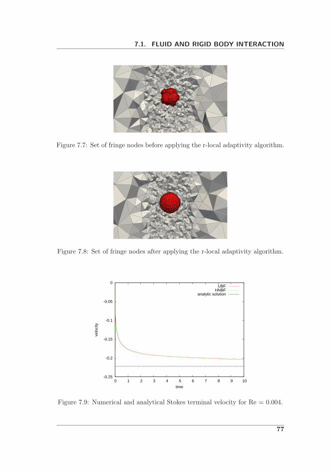
7.7 Set of fringe nodes before applying the r-local adaptivity algorithm. 77
7.8 Set of fringe nodes after applying the r-local adaptivity algorithm. 77
7.9 Numerical and analytical Stokes terminal velocity for Re = 0.004. 77
7.10 Linear and high order interpolation for the FMALE framework. . 78
7.11 Numerical and analytical terminal velocity for Re = 101. . . . . . 79
7.12 Numerical and analytical terminal velocity for Re = 1647. . . . . 79
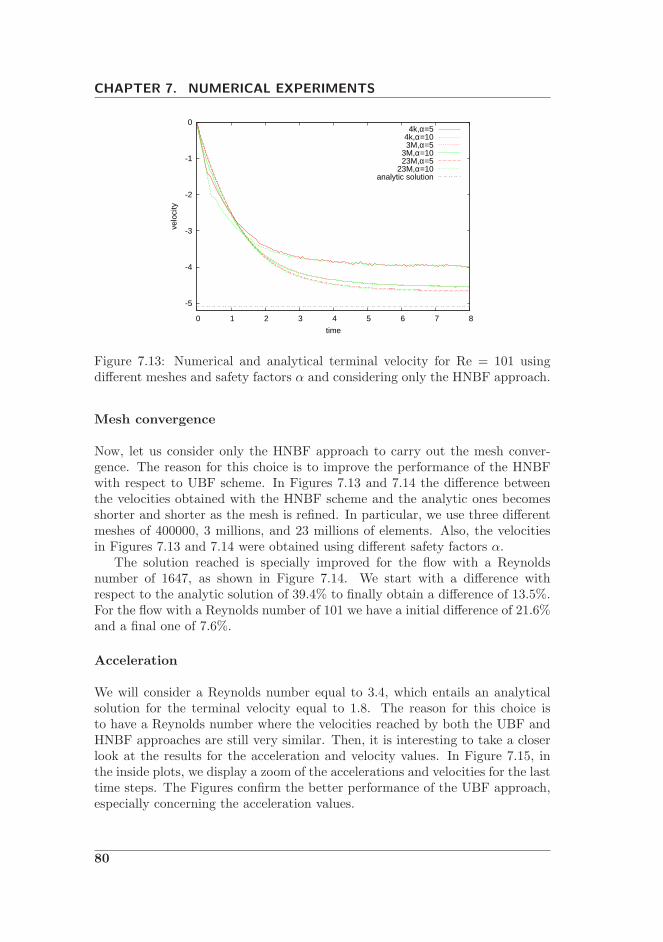
7.13 Numerical and analytical terminal velocity for Re = 101 usingdifferent meshes and safety factors α and considering only theHNBF approach. . . . . . . . . . . . . . . . . . . . . . . . . . . . 80
7.14 Numerical and analytical terminal velocity for Re = 1647 usingdifferent meshes and safety factors α and considering only theHNBF approach. . . . . . . . . . . . . . . . . . . . . . . . . . . . 81
7.15 Solid acceleration and solid velocity for the UBF and HNBF ap-proaches with Re=3.7. . . . . . . . . . . . . . . . . . . . . . . . . 81
7.16 Time step analysis using different safety factors for the UBFscheme with Re=101. . . . . . . . . . . . . . . . . . . . . . . . . 82
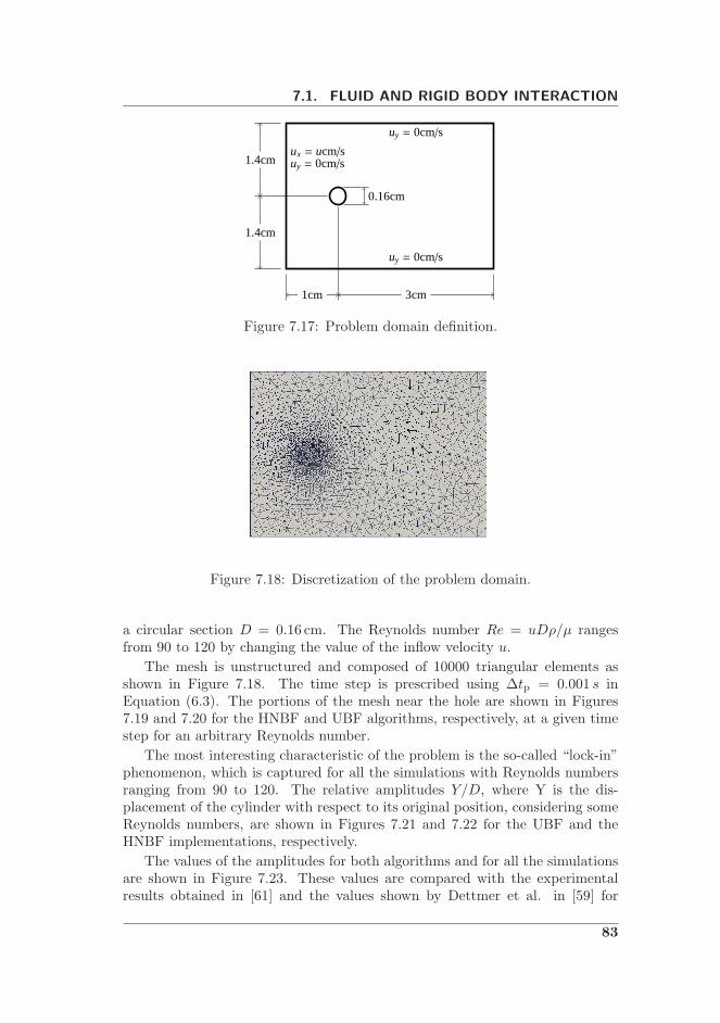
7.17 Problem domain definition. . . . . . . . . . . . . . . . . . . . . . 837.18 Discretization of the problem domain. . . . . . . . . . . . . . . . 837.19 Mesh near the hole for the high order kriging interpolation algo-
rithm. . . . . . . . . . . . . . . . . . . . . . . . . . . . . . . . . . 847.20 Mesh near the hole after applying the local r-adaptivity algorithm. 847.21 Amplitudes of the solid oscillations due to the vortex for the UBF
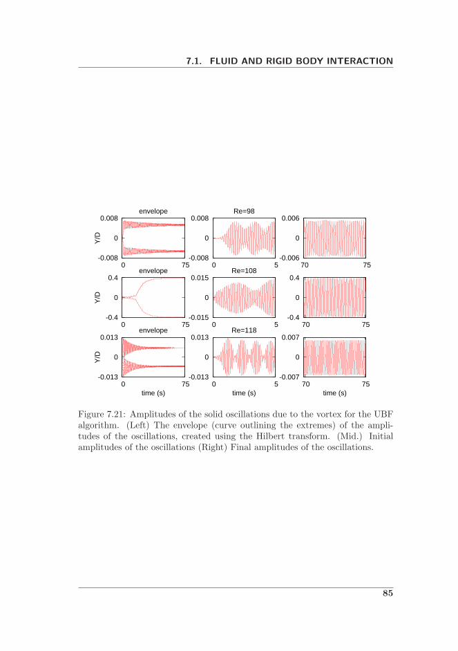
algorithm. (Left) The envelope (curve outlining the extremes)of the amplitudes of the oscillations, created using the Hilberttransform. (Mid.) Initial amplitudes of the oscillations (Right)Final amplitudes of the oscillations. . . . . . . . . . . . . . . . . . 85
7.22 Amplitudes of the solid oscillations due to the vortex for theHNBF algorithm. (Left) The envelope (curve outlining the ex-tremes) of the amplitudes of the oscillations, created using theHilbert transform. (Mid.) Initial amplitudes of the oscillations.(Right) Final amplitudes of the oscillations. . . . . . . . . . . . . 86
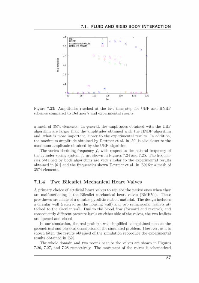
7.23 Amplitudes reached at the last time step for UBF and HNBFschemes compared to Dettmer’s and experimental results. . . . . 87
7.24 Frequencies reached at the last time step for UBF and HNBFschemes compared to experimental results. . . . . . . . . . . . . . 88
7.25 Frequencies reached at the last time step for UBF and HNBFschemes compared to Dettmer’s results. . . . . . . . . . . . . . . 88
7.26 Domain of the two bileaflet mechanical heart valves. A zoom isdone as shown in the square in Figure 7.27. . . . . . . . . . . . . 89
7.27 Zoom of the whole domain. Another zoom is done as shown inthe square in Figure 7.28. . . . . . . . . . . . . . . . . . . . . . . 89
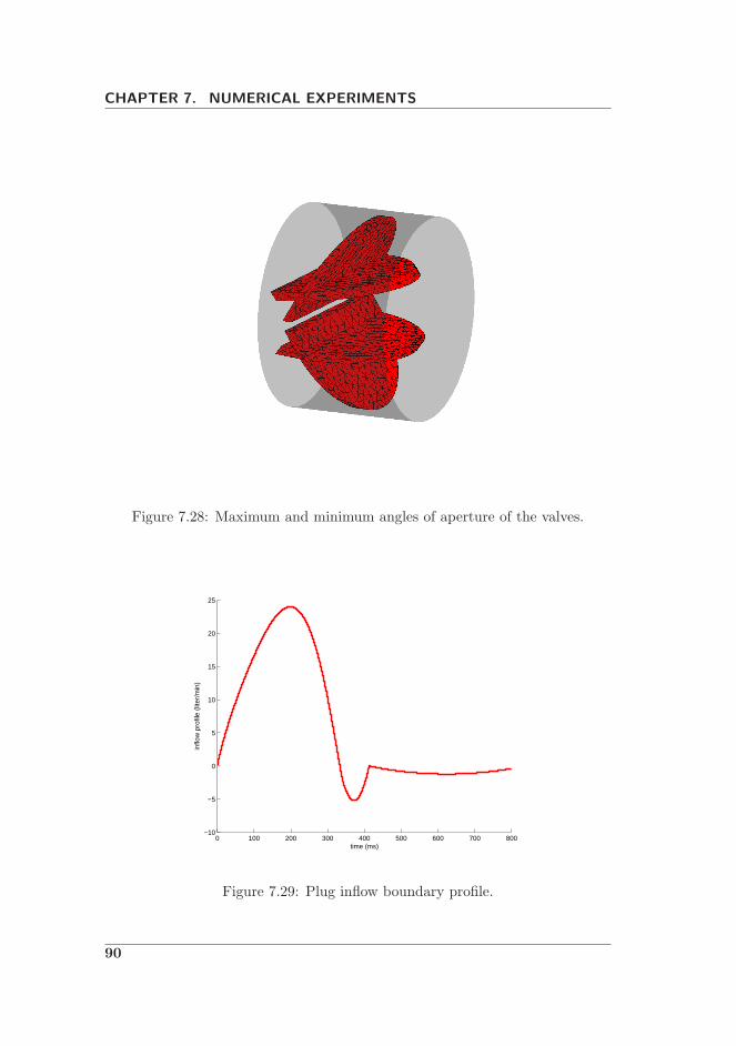
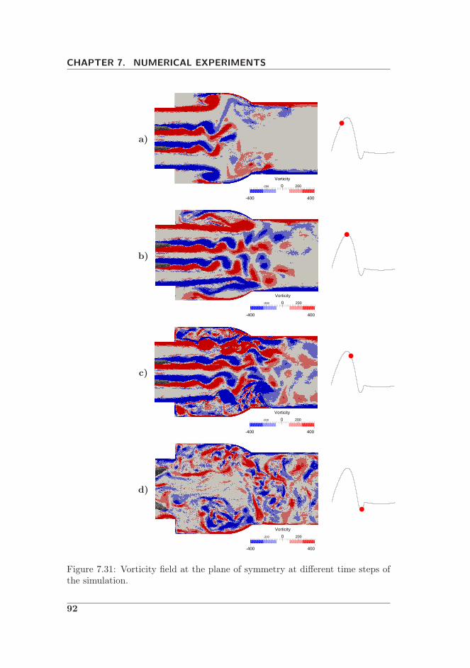
7.28 Maximum and minimum angles of aperture of the valves. . . . . 907.29 Plug inflow boundary profile. . . . . . . . . . . . . . . . . . . . . 907.30 Aperture angle of the valves. . . . . . . . . . . . . . . . . . . . . 917.31 Vorticity field at the plane of symmetry at different time steps of
the simulation. . . . . . . . . . . . . . . . . . . . . . . . . . . . . 927.32 One of the solids with arbitrary shape. . . . . . . . . . . . . . . . 937.33 The scalability using the NS equations solver with and without
considering the UBF and NBF algorithms. . . . . . . . . . . . . . 947.34 Fifty cubes falling into a funnel at the beginning of the simulation. 957.35 Fifty cubes falling into a funnel at the end of the simulation. . . 967.36 10000 spheres falling inside a square at the beginning of the sim-
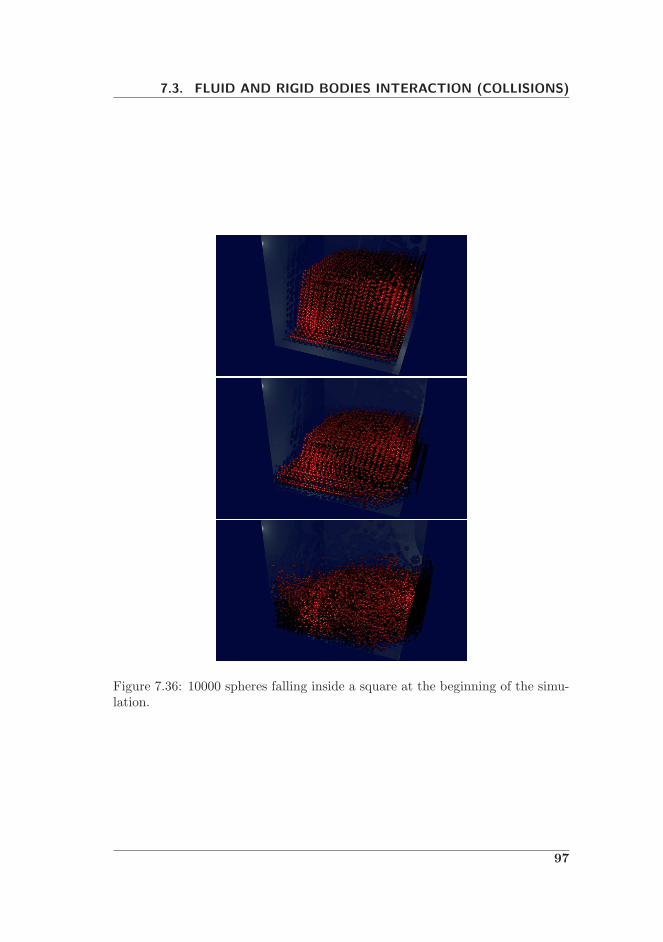
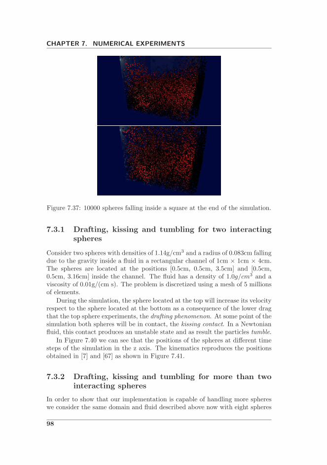
ulation. . . . . . . . . . . . . . . . . . . . . . . . . . . . . . . . . 977.37 10000 spheres falling inside a square at the end of the simulation. 98
7.38 4000 spheres crashing against the floor at the beginning of thesimulation. . . . . . . . . . . . . . . . . . . . . . . . . . . . . . . 99
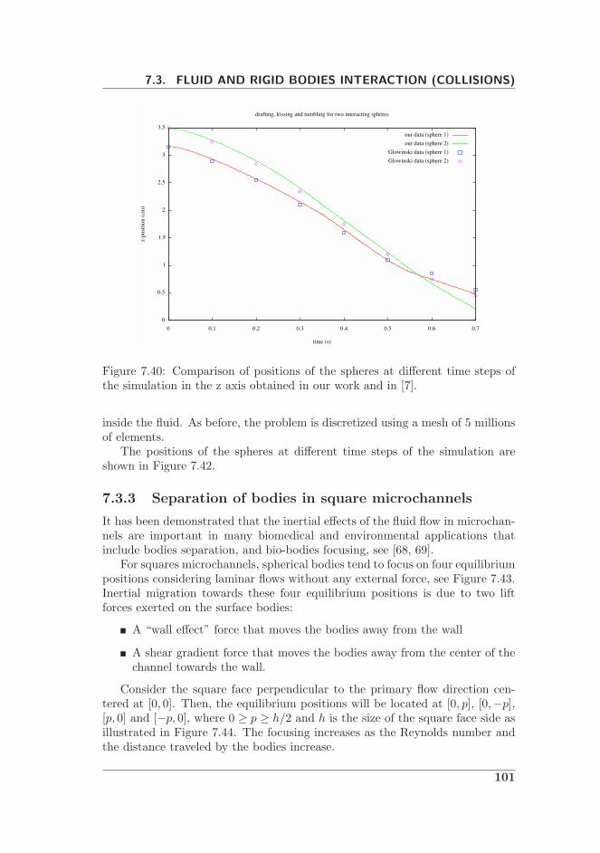
7.39 4000 spheres crashing against the floor at the end of the simulation.1007.40 Comparison of positions of the spheres at different time steps of
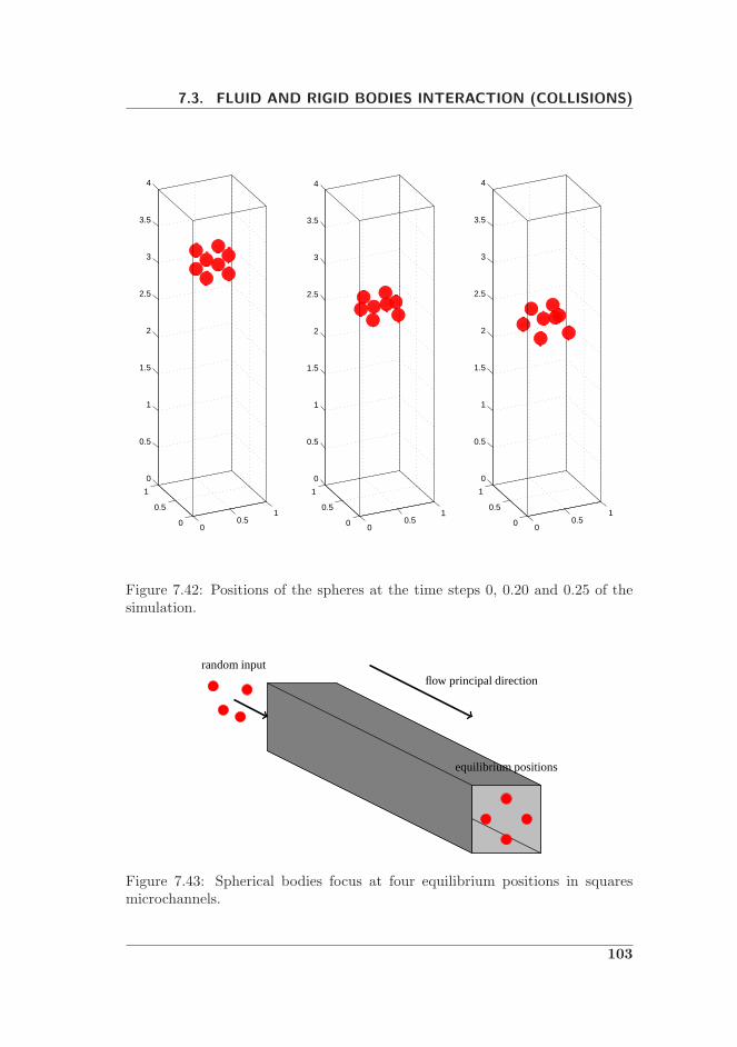
the simulation in the z axis obtained in our work and in [7]. . . . 1017.41 Positions of the spheres at different time steps of the simulation. 1027.42 Positions of the spheres at the time steps 0, 0.20 and 0.25 of the
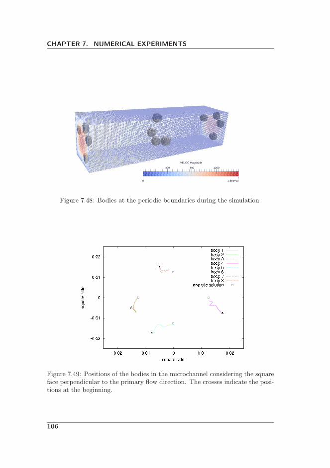
face perpendicular to the primary flow direction. . . . . . . . . . 1047.45 Considered periodic boundaries. . . . . . . . . . . . . . . . . . . . 1047.46 Added element and node connectivities for the periodic node n. . 1057.47 Body replication at the periodic boundaries. . . . . . . . . . . . . 1057.48 Bodies at the periodic boundaries during the simulation. . . . . . 1067.49 Positions of the bodies in the microchannel considering the square
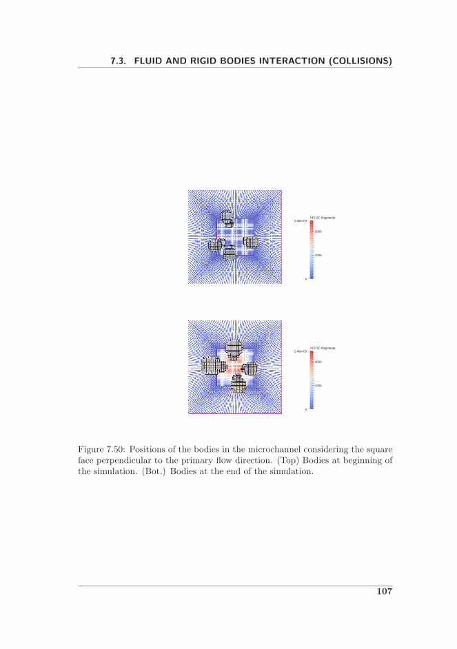
face perpendicular to the primary flow direction. The crossesindicate the positions at the beginning. . . . . . . . . . . . . . . . 106
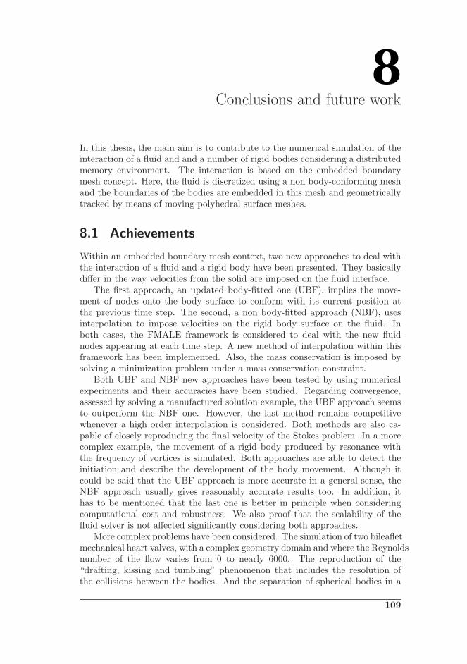
7.50 Positions of the bodies in the microchannel considering the squareface perpendicular to the primary flow direction. (Top) Bodiesat beginning of the simulation. (Bot.) Bodies at the end of thesimulation. . . . . . . . . . . . . . . . . . . . . . . . . . . . . . . 107
List of Algorithms
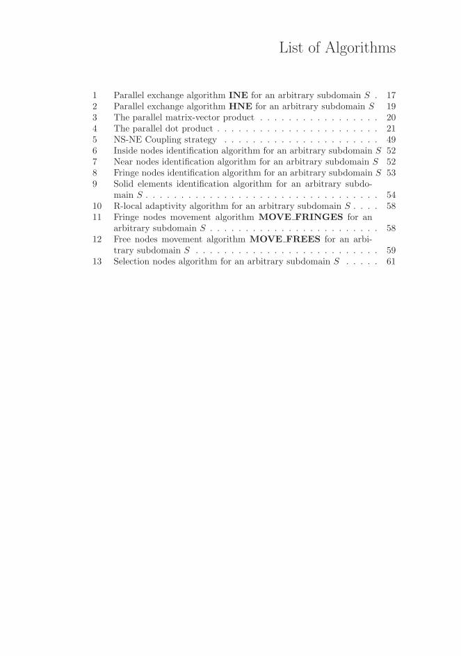
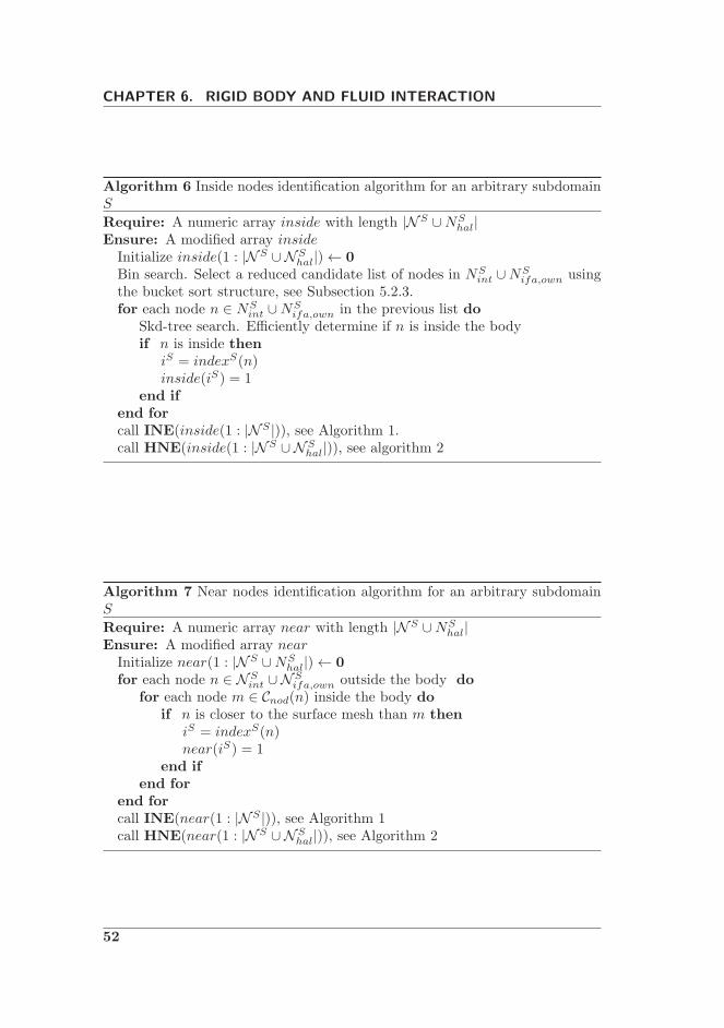
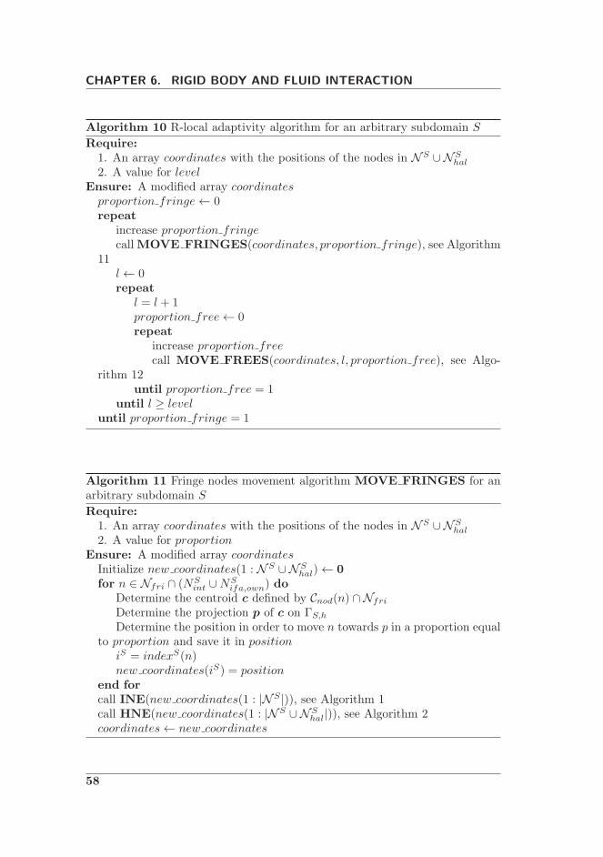
1 Parallel exchange algorithm INE for an arbitrary subdomain S . 172 Parallel exchange algorithm HNE for an arbitrary subdomain S 193 The parallel matrix-vector product . . . . . . . . . . . . . . . . . 204 The parallel dot product . . . . . . . . . . . . . . . . . . . . . . . 215 NS-NE Coupling strategy . . . . . . . . . . . . . . . . . . . . . . 496 Inside nodes identification algorithm for an arbitrary subdomain S 527 Near nodes identification algorithm for an arbitrary subdomain S 528 Fringe nodes identification algorithm for an arbitrary subdomain S 539 Solid elements identification algorithm for an arbitrary subdo-
main S . . . . . . . . . . . . . . . . . . . . . . . . . . . . . . . . . 5410 R-local adaptivity algorithm for an arbitrary subdomain S . . . . 5811 Fringe nodes movement algorithm MOVE FRINGES for an
arbitrary subdomain S . . . . . . . . . . . . . . . . . . . . . . . . 5812 Free nodes movement algorithm MOVE FREES for an arbi-
The numerical simulation of the interaction of a fluid and a rigid body in thecontext of high performance computing is a challenging subject. Efficiency istightly interlinked with a careful implementation. In this thesis we try to eluci-date the data structures and the algorithms that lead to an efficient simulationtool for supercomputers by means of formal definitions, thereby generating ageneral framework. The implementation of two embedded boundary methodsare described within this framework. They are implemented inside the Alyasystem [3], a parallel multiphysics code. Finally, several numerical examplesare used to demonstrate the accuracy and the computational efficiency of theimplemented methods.
1.1 Motivation
The detailed modeling of the interaction of a rigid solid with a fluid has beenthe object of intensive research [8, 9, 10, 11]. However, this is still a challengingsubject that entails several difficulties. The problem can become even harderwhen a high performance computing implementation is sought.
There exist different methods to simulate the interaction between the fluidand a solid in movement. We are mainly interested in techniques developedwithin the context of the Finite Element Method here. However, it is importantto mention other alternatives like those based on Lattice-Boltzman [12] andmeshless methods [13, 14, 15].
To put our work into context, the main approaches based on the FiniteElement Method are described below and schematized in Figure 1.1. This listis based on the review presented in [9].
• Domain decomposition methods [16]. Due to the actual process followedin this class of methods for fluid-structure interaction, maybe a more ap-propriate name is domain composition methods as pointed out in [17]. Afluid mesh attached to the body is moving over a fixed fluid mesh. Asa consequence, the information between adjacent meshes or subdomainshas to be exchanged to obtain a global solution. Several instances of thisapproach can be mentioned. The Chimera method [18, 19], and HER-MESH [20], are examples of partially overlapping domain decompositionas illustrated in Figure 1.1(Top)(Left). The sliding mesh method [21]is another example of domain decomposition; here the subdomains aredisjoint and information between them is transmitted across the inter-faces, see Figure 1.1(Top)(Right). In the shear-slip mesh update method(SSMUM) [8], a layer of shear-absorbing elements is used to connect a
1
CHAPTER 1. INTRODUCTION
Figure 1.1: Illustration of some methods to simulate flows around moving com-ponents. (Top) (Left) Chimera method. (Top) (Right) Sliding mesh method.(Mid.) (Left) SSMUM. (Mid.) (Right) ALE method (Bot.) Embedded bound-ary mesh.
moving, associated to the body, and non-moving region as illustrated inFigure 1.1(Mid.)(Left).
• The ALE method. The Arbitrary Lagrangian-Eulerian description (ALE)method takes advantage of the features of both (Lagrangian and Eulerian)descriptions to move the fluid mesh in order to adapt it to the changingsolid configuration [22]. Figure 1.1(Mid.)(Right) illustrates the movementof the mesh around a body in an ALE implementation. Remeshing isrequired when the elements in the discretization are too distorted.
• Embedded boundary methods. The fluid is discretized using a non body-conforming mesh and described in an Eulerian frame of reference. Thewet boundaries of the bodies are embedded in this mesh and geometri-cally tracked by means of moving polyhedral surface meshes, see Figure1.1(Bot.) Examples of this approach are the Immersed Boundary (IB)method [23] and the Fictitious Domain (FD) [24, 25]. Another examplerelevant to this work is the strategy proposed by Lohner et al. [26], whichimposes the velocity of the body directly as a Dirichlet boundary conditionon the fluid. There exist other alternatives such as the work developed in[27] that combines concepts from embedded boundary methods and theisogeometric analysis introduced in [28].
• Monolithic approach. A unified formulation is used for both the solid and
2
1.1. MOTIVATION
fluid. Interaction is taken into account by means of an extra stress tensorappearing in the Navier-Stokes equations [10].
Within this context, the two new schemes proposed in this work can becharacterized as based on the embedded boundary concept. They both managean internal boundary in the fluid domain at each time step to track the solidwet boundary.
The selection of the strategies has been motivated by the search of a com-putationally efficient parallel implementation. We decided to avoid connectingdifferent meshes, because it implies changing the nodes connectivities, therebyincreasing parallel communications and the complexity of the algorithms. Alter-natives that can cause severe distortions in some elements were also avoided. Inorder to tackle these distortions, re-meshing can be used, but this would entailthe need of changing nodes connectivities, which would require redistributingthe computational load in the mesh partitions. That is why we avoid changesin the topology of the mesh in both of the proposed approaches.
To account for the fact that fluid nodes can become solid nodes and viceversa due to the rigid body movement, we have adopted the FMALE approach[29, 30]. A new interpolation method is adopted inside the FMALE implemen-tation in order to improve the results. Also, to track the wet boundary of thebody, computational geometry tools have been used. In general, the two newapproaches, in order to be both computationally efficient and accurate, entailthe integration of different algorithmic solutions.
In addition, in a simulation of a dynamic rigid body system multiple prob-lems have to be solved. First, the motion of bodies due to the external forcesmust be determined. Next, when the bodies are in movement, it is necessaryto prevent interpenetration between them and to solve the collisions when thebodies are in contact. The simulation framework of dynamic rigid bodies iswell-known, see [31, 32], and tries to solve the problems mentioned above in thefollowing consecutive stages:
• Collision Detection.
• Rigid Body Motion.
• Collision Response.
The previous paragraphs can give the reader a hint of the intrinsic complex-ity associated to obtaining an efficient parallel implementation of the interactionof a fluid and a rigid body. This complexity is reflected in the difficulty of giv-ing an accurate explanation of such implementations. This is why the need ofgenerating a framework that allows for a precise description was felt. A very in-teresting attempt to create such a framework for the modeling of incompressibleflows can be found in [33, 34]. However, in the author’s opinion, a new frame-work better suited for fluid-structure interaction (FSI) was necessary. Thus,a new formal characterization of the data structures needed in a distributedmemory environment in terms of set theory concepts is introduced. It must
3
CHAPTER 1. INTRODUCTION
be said that the parallel framework, although mainly thought for FSI, can begeneralized to other applications. In [2], some elements of this framework wereused to explain a parallel solver for solid mechanics.
1.2 Objectives
The aim of this thesis is to numerically simulate the interaction of a fluid anda number of rigid bodies considering a distributed memory environment. Toachieve this goal, we have to accomplish the objectives mentioned below.
In order to have a precise description of the parallel algorithms to solve theinteraction:
• To develop a general framework for the parallel implementation of theinteraction between a fluid and the rigid bodies by means of a new formaldefinition using the set notation. This general framework is intended toelucidate the data structures and algorithms involved in a precise fashion.The main formal definitions are detailed in Chapter 2.
In order to numerically solve the interaction inside the embedded boundarymesh framework:
• To propose two new strategies to accurately solve the interaction of afluid and a number of rigid bodies inside the embedded boundary meshframework considering a distributed memory parallelization environment.The description is detailed in Subsection 6.2.2. The validation of bothapproaches is described in Subsection 7.1.1.
• To adopt a new interpolation method inside the FMALE framework inorder to account for the fact that fluid nodes can become solid nodes andvice versa due to the rigid body movement. The FMALE framework isexplained in Subsection 6.2.3. The new method of interpolation is studiedin Subsection 7.1.2.
• To solve the interactions between the bodies. As all the subdomains sim-ulate the interaction of all the bodies and redundant work is done, theimplementation has to be done in such way that each subdomain solvesthese interactions as fast as possible. The theory is described in Chapter5. Some examples are shown in Section 7.2.
Finally, in order to implement the interaction to solve real problems:
• To select numerical strategies motivated by the search of a computation-ally efficient parallel implementation.
4
1.3. LIMITATIONS
1.3 Limitations
We do not know the positions of the bodies inside the mesh that discretizes theproblem a priori. Thus, in general, the discretization of a problem entails a finemesh in order to obtain results that are good enough.
The mesh has to become finer as the Reynolds number increases. To solveturbulent flows, the required mesh could imply a considerable growth in thenumber of degrees of freedom and alternative numerical methods, that includenumerical strategies to simulate flows with high Reynolds numbers, can renderbetter solutions for this kind of problems with coarser meshes. Remeshing canbe used, but, as mentioned above in Section 1.1, this would require redistribut-ing the computational load in the mesh partitions.
For all these reasons, in this thesis, the analyses will be focused on laminarand transition flows. In particular, flows with Reynolds numbers until nearly6000. The discretization of the problems will use meshes of until nearly 30million elements. Even so, the sizes of the meshes and the time of simulationrequire a distributed memory environment to solve the problems considered inthis work. In this context, our main goal is not to affect the scalability ofthe Alya system. That is, not to affect the scalability of the fluid solver. Ananalysis of the scalability of the implementation for the proposed new strategiesis described in Subsection 7.1.5.
1.4 Outline of the thesis
The rest of this thesis is organized as follows. Chapter 2 is devoted to ex-plaining the mesh topology structures considering a parallel context. Also, thealgorithms to exchange the data structures associated to this mesh are explainedinside a parallel finite element and a parallel finite difference implementations.The physics and numerical aspects to solve a fluid and a rigid body are describedrespectively in Chapters 3 and 4. The general framework of interaction betweenrigid bodies is explained in Chapter 5. The Chapter 6 describes in detail a gen-eral algorithm to solve the interaction between a fluid and a rigid body. It isimportant to remark that all the algorithms derived from the general algorithmare described considering a parallel implementation and using the algorithms ofexchange explained in Chapter 2.
The numerical examples are presented in Chapter 7 in order to validate themethods. Finally, the conclusions of this work are presented in Chapter 8.
5
2Parallel context
In a parallel finite element program, the original mesh is partitioned into subdo-mains. The data that has a direct relationship with the set of nodes of the meshwill be also divided. As a consequence, the data between adjacent subdomainshas to be exchanged to preserve the coherency of the data and to obtain thecorrect solution to the problem.
In order to be precise and avoid ambiguities, some sets are defined to repre-sent the original mesh, first, in a serial context, and then, in a parallel context.To illustrate the concepts, a simple one-dimensional example will be considered.
Then, a formal description of the algorithms to exchange data in a finiteelement or a finite difference parallel program will be described. A simple iter-ation of an iterative solver will be considered in order to motivate the definitionof the algorithms.
2.1 Finite Element Serial Context
In the context of the finite element method, the continuous domain is discretizedinto a set of elements E = e1, e2, e3, ... and a set of nodes N = n1, n2, n3, ....Each node n ∈ N is defined by its position inside the domain. And eachelement e ∈ E is defined, for our purposes, by a subset of the set of nodese = ne
1, ne2, n
e3, ... ⊂ N .
Mesh connectivities
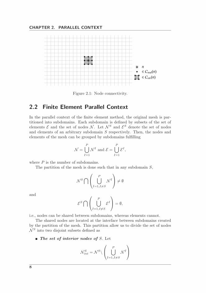
The definition of an element as a subset of nodes relates any node n ∈ Nwith other nodes and elements of the mesh. These relations are called theconnectivity of node n and can be characterized by the following definitions:
• Element connectivity of n. Let Cele(n) denote the set of elements in Edirectly connected to the node n, the gray squares in Figure 2.1. Formally,
Cele(n) = e ∈ E : n ∈ e.
• Node connectivity of n. Let Cnod(n) denote the set of nodes in Ndirectly connected to n, the black circles in Figure 2.1. Formally,
Cnod(n) = m ∈ N : ∃e ∈ Cele(n),m ∈ e \n.
7
CHAPTER 2. PARALLEL CONTEXT
n∈ Cnod(n)
∈ Cele(n)
Figure 2.1: Node connectivity.
2.2 Finite Element Parallel Context
In the parallel context of the finite element method, the original mesh is par-titioned into subdomains. Each subdomain is defined by subsets of the set ofelements E and the set of nodes N . Let N S and ES denote the set of nodesand elements of an arbitrary subdomain S respectively. Then, the nodes andelements of the mesh can be grouped by subdomains fulfilling
N =
P⋃
I=1
N I and E =
P⋃
I=1
EI ,
where P is the number of subdomains.The partition of the mesh is done such that in any subdomain S,
N S⋂
P⋃
I=1,I 6=S
N I
6= ∅
and
ES⋂
P⋃
I=1,I 6=S
EI
= ∅,
i.e., nodes can be shared between subdomains, whereas elements cannot.The shared nodes are located at the interface between subdomains created
by the partition of the mesh. This partition allow us to divide the set of nodesN S into two disjoint subsets defined as
The set of interior nodes of S. Let
N Sint = N
S\
P⋃
I=1,I 6=S
N I
8
2.2. FINITE ELEMENT PARALLEL CONTEXT
S T
∈ NSi f a
∈ NSint
Figure 2.2: Interface and interior nodes of the subdomain S.
denote the set of interior nodes of the subdomain S. These nodes donot belong to the interface; see Figure 2.2, where white circles denote theinterior nodes of S.
The set of interface nodes of S. Let N Sifa = N S\N S
int denote theset of interface nodes of S. These nodes belong to the interface and areshared by different subdomains, including S; see Figure 2.2, where blackcircles denote the interface nodes of S.
Two arbitrary subdomains S and T that share at least one node at theinterface are called as adjacent subdomains, i.e N S
ifa ∩ NTifa 6= ∅. Consider
the partition shown in Figure 2.2. In this particular example, the subdomainsS and T are adjacent because they share a set of interface nodes.
Let us define a useful subset of the interface nodes N Sifa that will be used in
most of the parallel algorithms for fluid and rigid body interaction describe inthis thesis:
The set of own interface nodes of S. Let N Sifa,own denote the own
interface nodes of a subdomain S. These own nodes are uniquely associ-ated to a subdomain in order to manage communications properly whenperforming certain operations. The definition of the set of own interfacenodes of S states that:
N Sifa,own ∩
⋃
I 6=S,I is adjacent to S
N Iifa,own = ∅.
That is, an own interface node of S cannot be own by another subdomaindifferent from S.
Parallel mesh connectivity
In this context, consider a node n in an arbitrary subdomain S that is locatedat the interface. From the point of view of subdomain S, there are two disjointsets whose union defines the whole node connectivity of n:
9
CHAPTER 2. PARALLEL CONTEXT
• Node connectivity of n in S. Let the set
CSnod(n) = Cnod(n) ∩ NS
denote the set of nodes in N S directly connected to the node n.
• Node connectivity of n in other subdomains. Let the set
CSnod(n) = Cnod(n)\CSnod(n)
denote the set of nodes in subdomains different from S directly connectedto the node n. These nodes will be referred to as halo nodes of S, seeSection 2.4.
In a similar way, there are two disjoint sets whose union defines the wholeelement connectivity of n:
• Element connectivity of n in S. Let the set
CSele(n) = Cele(n) ∩ ES
denote the set of elements in ES directly connected to the node n.
• Element connectivity of n in other subdomains. Let the set
CSele(n) = Cele(n)\CSele(n)
denote the set of element in subdomains different from S directly con-nected to the node n. These elements will be referred to as halo elements
of S, see Section 2.4.
In Figure 2.3, the whole connectivity of the interface node n is dividedbetween the adjacent subdomains S and T .
2.3 Finite Element and Finite Difference Parallel Ex-
change
In a distributed memory context, a typical parallel implementation of the finiteelement (FE) method differs from a typical parallel implementation of the fi-nite difference (FD) or the finite volume (FV) method. The difference stemsfrom the way these methods assemble the algebraic systems resulting from thediscretizations. On the one hand, in a finite difference code (similarly in a FVcode), each process is responsible for a given set of rows of the matrix. In orderto complete each row, a subdomain is defined by a subset of the set of nodes ofthe original mesh and by the set of edges that are directly connected with this
10
2.3. FINITE ELEMENT AND FINITE DIFFERENCE PARALLELEXCHANGE
S T
n ∈ CTnod(n)
∈ CTele(n)
∈ CSnod(n)
∈ CSele(n)
Figure 2.3: Node connectivity in a parallel context.
subset of nodes. Thus, the edges located at the interface between subdomains(cells in a FV code) are duplicated, resulting in an overlap of edges (cells), seeFigure 2.4. On the other hand, in a finite element code, a subdomain is definedby a subset of the set of elements of the original mesh and by the set of nodesthat belongs to this subset of elements, see also Figure 2.4. Only the nodeslocated at the interface between subdomains are duplicated and on these nodes,the matrix is assembled locally and only partly on each subdomain. To illus-trate this fact, let us take a very simple one-dimensional example. Figure 2.4shows the partition of the mesh into two subdomains, S and T . In the case ofthe FD method, edge n3−n4 is duplicated. Subdomain S is responsible for therows of nodes n1,n2 and n3 while subdomain T takes care of nodes n4 and n5.In the case of the finite element method, no element is duplicated. But bothsubdomains will partly be responsible for node n3. Now let us examine how theparallelization works.
Finite difference method
subdomainS
subdomainT
duplicate edge
n1 n2 n3 n4
n3 n4 n5
Finite element method
subdomainS
subdomainT
duplicate node
n1 n2 n3
n3 n4 n5
Figure 2.4: Mesh partition for FD and FE.
11
CHAPTER 2. PARALLEL CONTEXT
The numerical solution of a PDE (and consequently the Navier-Stokes equa-tions) consists mainly of two steps. First, the construction of the matrix A andright-hand side (RHS) b of the algebraic system Ax = b. Second, the solutionof this system using an iterative solver. As far as the matrix and RHS assem-blies are concerned, in the case of the FD and FV methods, each subdomain isable to construct complete rows and RHS thanks to the duplicated edges (cellsin a FV code). In the case of the finite element method, only part of the matrixis assembled for the interface nodes. As far as iterative solvers are concerned,the basic operation is the matrix-vector product. Let us consider the matrix-product y = Ax and examine the parallelization of this product for the FD andFE methods; see Figure 2.5.
Finite difference method
1. Exchange: S sends x3 to T
2. Exchange: T sends x4 to S
3. Local matrix-vector product
y1
y2
y3
=
A11 A12
A21 A22 A23
A32 A33 A34
x1
x2
x3
x4
y4
y5=
A43 A44 A45
A54 A55
x3
x4
x5
Finite element method
1. Local matrix-vector product
y1
y2
yS3
=
A11 A12
A21 A22 A23
A32 AS33
x1
x2
x3
yT3
y4
y5
=
AT33
A34
A43 A44 A45
A54 A55
x3
x4
x5
2. Exchange: S sends yS3 to T
3. Exchange: T sends yT3 to S
4. Assembly: y3 = yS3 + yT3
Figure 2.5: Parallel matrix-vector product for FD and FE.
In the FD case, on the one hand, subdomain S is in charge of the whole rowof node n3. Thanks to the duplication of edge n3−n4, coefficients A33 and A34
are complete. On the other hand, subdomain T is in charge of the whole row ofnode n4. As before, thanks to the duplication of edge n3 − n4, coefficients A43
and A44 are complete. The matrix-vector product can be carried out in parallelas follows:
1. Exchange the data x3 and x4 between the subdomains S and T .
2. Perform local matrix-vector product.
In the case of the FE, the coefficients of the matrix come from element inte-grals. Subdomain S can therefore provide only part of coefficient A33, namelyAS
33, while subdomain T provides AT33. Note that
y3 = A32x2 +A33x3 +A34x4
12
2.4. HALO NODES AND HALO ELEMENTS
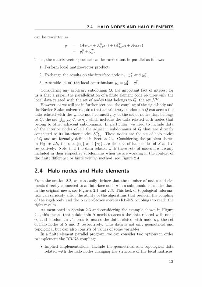
can be rewritten as
y3 = (A32x2 +AS33x3) + (AT
33x3 +A34x4)
= yS3 + yT3 .
Then, the matrix-vector product can be carried out in parallel as follows:
1. Perform local matrix-vector product.
2. Exchange the results on the interface node n3: yS3 and yT3 .
3. Assemble (sum) the local contribution: y3 = yS3 + yT3 .
Considering any arbitrary subdomain Q, the important fact of interest forus is that a priori, the parallelization of a finite element code requires only thelocal data related with the set of nodes that belongs to Q, the set NQ.
However, as we will see in further sections, the coupling of the rigid-body andthe Navier-Stokes solvers requires that an arbitrary subdomain Q can access thedata related with the whole node connectivity of the set of nodes that belongsto Q, the set
⋃
n∈NQ Cnod(n), which includes the data related with nodes thatbelong to other adjacent subdomains. In particular, we need to include dataof the interior nodes of all the adjacent subdomains of Q that are directlyconnected to its interface nodes NQ
ifa. These nodes are the set of halo nodesof Q and are formally defined in Section 2.4. Considering the problem shownin Figure 2.5, the sets n4 and n2 are the sets of halo nodes of S and Trespectively. Note that the data related with these sets of nodes are alreadyincluded in their respective subdomains when we are working in the context ofthe finite difference or finite volume method, see Figure 2.4.
2.4 Halo nodes and Halo elements
From the section 2.2, we can easily deduce that the number of nodes and ele-ments directly connected to an interface node n in a subdomain is smaller thanin the original mesh, see Figures 2.1 and 2.3. This lack of topological informa-tion can seriously affect the ability of the algorithms that perform the couplingof the rigid-body and the Navier-Stokes solvers (RB-NS coupling) to reach theright results.
As mentioned in Section 2.3 and considering the example shown in Figure2.4, this means that subdomain S needs to access the data related with noden4 and subdomain T needs to access the data related with node n3, the setof halo nodes of S and T respectively. This data is not only geometrical andtopological but can also consists of values of some variables.
In a finite element parallel program, we can consider two options in orderto implement the RB-NS coupling:
• Implicit implementation. Include the geometrical and topological datarelated with the halo nodes changing the structure of the local matrices.
13
CHAPTER 2. PARALLEL CONTEXT
In this case, the implementation have to enable rectangular matrices likein the case of the FD method in order to implicit the relation with thehalo nodes.
• Explicit implementation. Include the geometrical and topological datarelated with the halo nodes without changing the structure of the localmatrices. In this case, we lose in convergence as the values of the variablesrelated with the halo nodes have to go to the RHS.
In our code, we choose the explicit implementation option in order to preservethe structure of the local matrices. Some geometrical and topological data isadded in the subdomain definitions in order to have the same connectivity asin the original mesh for any interface node.
From the point of view of an arbitrary subdomain S, the formal definitionsof these new added sets of nodes and elements are given by:
• Set of halo nodes of S. Let the set
N Shal =
⋃
n∈NSifa
CSnod(n)
denote the set of halo nodes in S.
• Set of halo elements of S. Let the set
EShal =⋃
n∈NSifa
CSele(n)
denote the set of halo elements in S.
Consider again the connectivity of the interface node n in Figure 2.3. Now,if we include the halo nodes and halo elements of the subdomain S, as shownin Figure 2.6, the interface node n in Figure 2.3 or any other interface node inthe subdomain S, will have defined its whole connectivity inside S.
2.5 Parallel exchange algorithms
In a finite element program, the most important data structures have a directrelationship with the set of nodes of the mesh. These structures are collectionsof numerical values, each one identified by an index (or a tuple of indices). Ina parallel context, these data structures have to be exchanged between subdo-mains to preserve the coherency of the data.
In parallel, for any subdomain S, a node in N S ∪N Shal is related to its index
by:
indexS : N S ∪ N Shal → 1, 2, 3, ...|N S ∪N S
hal|
n 7→ iS .
14
2.5. PARALLEL EXCHANGE ALGORITHMS
S T
∈ NSi f a
∈ NShal
∈ EShal
Figure 2.6: Halo nodes and halo element of subdomain S.
For implementation aspects, a subdomain S enumerates consecutively itsinterior nodes, next its own interface nodes, the rest of its interface nodes, andfinally its halo nodes, see Figure 2.7. Thus, any numerical data array dataof length |N S ∪ N S
hal| can be conveniently splitted in four consecutive arrays:data(1 : |N S
int|), the values related with the interior nodes of S, data(|N Sint| +
1 : |N Sint ∪ N
Sifa,own|), the values related with the own interface nodes of S,
data(|N Sint ∪ N
Sifa,own| + 1 : |N S |), the values related with the interface nodes
that do not own S, and data(|N S |+1 : |N S∪N Shal|), the values related with the
halo nodes of S. Also, these divisions facilitate the definition of the algorithmswritten above which allow us to exchange data between subdomains.
2.5.1 Interface node exchange algorithm (INE)
Consider an arbitrary subdomain S. Then, for each adjacent subdomain T ofS, the algorithm carries out the exchange of values associated with the subsetof interface nodes N S ∩ N T . For this purpose, the algorithm needs a commonindex in S and T as defined below:
indexS,Tifa : N S ∩ N T → 1, 2, 3, ...|N S ∩ N T |
n 7→ iS,Tifa .
The exchange of data is described in Algorithm 1. Considering the twoadjacent subdomains S and T shown in Figure 2.8, this exchange involves thedata related with the black nodes shown in Figure 2.8 and can be schematizedas illustrated in Figure 2.9.
From the point of view of an arbitrary node n ∈ N Sint, the Algorithm 1 works
as explained next. Let the contributions of a variable x evaluated at node nfurnished by S and all its adjacent subdomains A1, A2, ..., AN that share n;
that is n ∈ NA1
, n ∈ NA2
, ..., n ∈ NAN
; be denoted by xS and x1, x2, ..., xN
respectively. The Algorithm 1, first exchanges the values x1, x2, ..., xN and xS
15
CHAPTER 2. PARALLEL CONTEXT
|NS ∪NShal|
...
|NS |+ 1
|NS |
...
|NSint ∪NS
ifa,own|+ 1
|NSint ∪NS
ifa,own|
...
|NSint|+ 1
|NSint|
...
2
1
halo nodes of S
interface nodes not owned by S
own interface nodes of S
interior nodes of S
Figure 2.7: Array of data related with the set of nodes of S.
S
T
∈ NS ∩NT
Figure 2.8: Adjacent subdomains S and T .
MPI SendRecv
S
T
NS ∩NT
Figure 2.9: Interface nodes parallel exchange.
16
2.5. PARALLEL EXCHANGE ALGORITHMS
between the subdomains A1, A2, ..., AN and S. Then, the Algorithm 1 adds thecontribution coming from the subdomains A1, A2, ..., AN to get a new value
associated to n in S equal to xS +
N∑
I=1
xI .
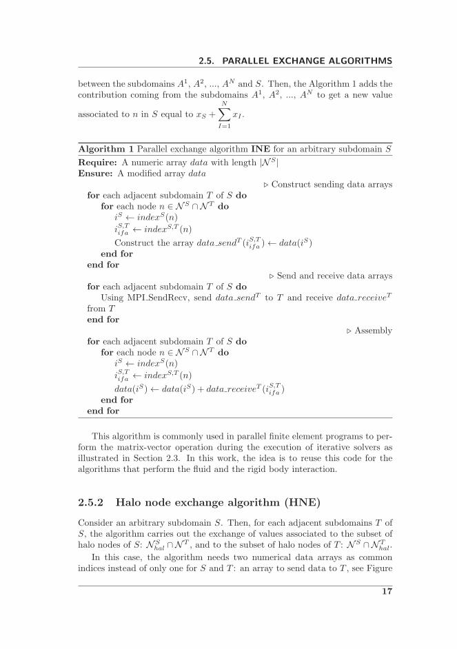
Algorithm 1 Parallel exchange algorithm INE for an arbitrary subdomain S
Require: A numeric array data with length |N S |Ensure: A modified array data
⊲ Construct sending data arraysfor each adjacent subdomain T of S do
for each node n ∈ N S ∩ N T doiS ← indexS(n)
iS,Tifa ← indexS,T (n)
Construct the array data sendT (iS,Tifa )← data(iS)end for
end for⊲ Send and receive data arrays
for each adjacent subdomain T of S doUsing MPI SendRecv, send data sendT to T and receive data receiveT
from Tend for
⊲ Assemblyfor each adjacent subdomain T of S do
for each node n ∈ N S ∩ N T doiS ← indexS(n)
iS,Tifa ← indexS,T (n)
data(iS)← data(iS) + data receiveT (iS,Tifa )end for
end for
This algorithm is commonly used in parallel finite element programs to per-form the matrix-vector operation during the execution of iterative solvers asillustrated in Section 2.3. In this work, the idea is to reuse this code for thealgorithms that perform the fluid and the rigid body interaction.
2.5.2 Halo node exchange algorithm (HNE)
Consider an arbitrary subdomain S. Then, for each adjacent subdomains T ofS, the algorithm carries out the exchange of values associated to the subset ofhalo nodes of S: N S
hal ∩NT , and to the subset of halo nodes of T : N S ∩N T
hal.
In this case, the algorithm needs two numerical data arrays as commonindices instead of only one for S and T : an array to send data to T , see Figure
17
CHAPTER 2. PARALLEL CONTEXT
S
T
∈ NS ∩NThal
∈ NShal ∩ N
T
Figure 2.10: Adjacent subdomains S and T .
MPI Sendv
S
T
NS ∩NThal
Figure 2.11: Halo nodes parallel exchange. Send data from S to T .
2.11, and another one to receive data from T , see Figure 2.12. From S to T :
indexS,Thal : N S ∩ N T
hal → 1, 2, 3, ...|N S ∩ N Thal|
n 7→ iS,T .
From T to S:
indexT,Shal : N T ∩ N S
hal → 1, 2, 3, ...|N T ∩ N Shal|
n 7→ iT,S .
The exchange is described in Algorithm 2. Considering the two adjacentsubdomains S and T shown in Figure 2.10, the exchange of data involves thedata related with the black and white nodes shown in Figure 2.10 and can beschematized as illustrated in Figures 2.11 and 2.12. In Figure 2.11 the data issent from S to T and in Figure 2.12 the data is sent from T to S.
From the point of view of an arbitrary node n ∈ N Shal that is shared with an
adjacent subdomain T of S, that is n ∈ N T , the Algorithm 2 works as explainednext. Let the values associated to n be xS and xT for S and T respectively.The Algorithm 2, first, sends the value xT from T to S and, then, replaces thevalue associated to n in S to get a new value xS = xT .
Actually, the relationships between a subset of nodes and a common indexfor a pair of adjacent subdomains defined above are slightly different in the
18
2.5. PARALLEL EXCHANGE ALGORITHMS
MPI Recv
S
T
NShal ∩N
T
Figure 2.12: Halo nodes parallel exchange. Receive data from T in S.
Algorithm 2 Parallel exchange algorithm HNE for an arbitrary subdomain S
Require: A numeric array data with length |N S ∪ N Shal|
Ensure: A modified array data⊲ Construct sending data arrays
for each adjacent subdomain T of S dofor each node n ∈ N S ∩ N T
hal doiS ← indexS(n)
iS,Thal ← indexS,Thal (n)
Construct the array data sendT (iS,Thal )← data(iS)end for
end for⊲ Send and receive data arrays
for each adjacent subdomain T of S doUsing MPI Send, send data sendT to TUsing MPI Recv, receive data receiveT from T
end for⊲ Data substitution
for each adjacent subdomain T of S dofor each node n ∈ N T ∩ N S
hal doiS ← indexS(n)
iT,Shal ← indexT,S(n)
data(iS)← data receiveT (iT,Shal )
end forend for
19
CHAPTER 2. PARALLEL CONTEXT
implementation level. The idea is to avoid to send or to receive redundant data.Thus, the value of a node n ∈ N S
hal shared for the adjacent subdomains of S:
A1, A2, ..., AN ; that is n ∈ NA1
, n ∈ NA2
, ..., n ∈ NAN
; will be sent only
for the adjacent subdomain NAI
, where 1 ≤ I ≥ N , with the smaller identifiervalue.
2.5.3 Parallel matrix-vector and dot product
To describe some characteristics of the iterative methods for solving linear sys-tems in a parallel context, consider a simple iteration of an Orthomin(1) method:
xk+1 = xk + α(
b−Axk)
,
where k is the iteration index, α =< rk,Ark > / < Ark,Ark >, and rk =b−Axk.
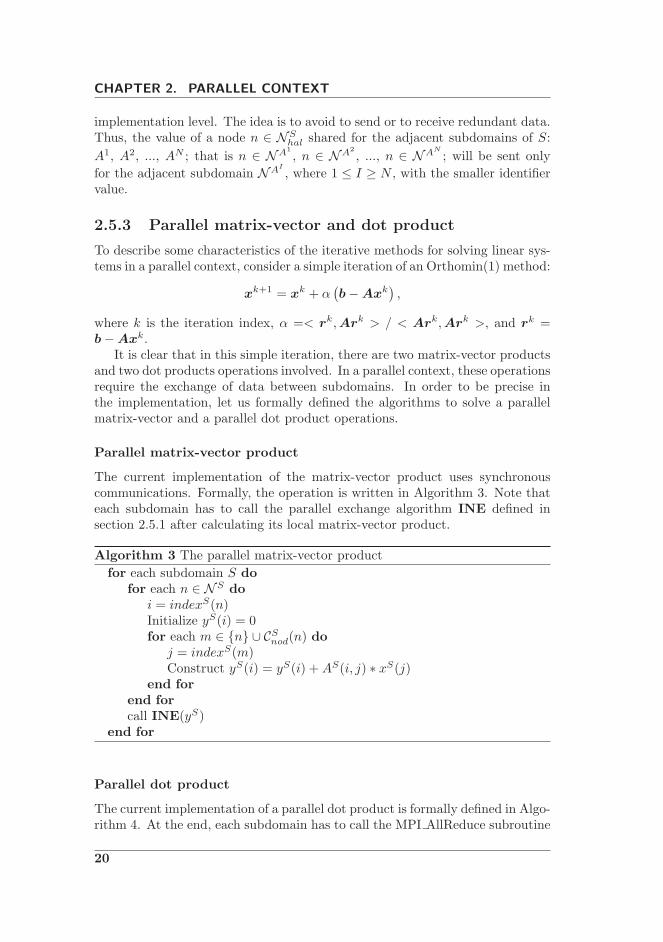
It is clear that in this simple iteration, there are two matrix-vector productsand two dot products operations involved. In a parallel context, these operationsrequire the exchange of data between subdomains. In order to be precise inthe implementation, let us formally defined the algorithms to solve a parallelmatrix-vector and a parallel dot product operations.
Parallel matrix-vector product
The current implementation of the matrix-vector product uses synchronouscommunications. Formally, the operation is written in Algorithm 3. Note thateach subdomain has to call the parallel exchange algorithm INE defined insection 2.5.1 after calculating its local matrix-vector product.
Algorithm 3 The parallel matrix-vector product
for each subdomain S dofor each n ∈ N S do
i = indexS(n)Initialize yS(i) = 0for each m ∈ n ∪ CSnod(n) do
The current implementation of a parallel dot product is formally defined in Algo-rithm 4. At the end, each subdomain has to call the MPI AllReduce subroutine
20
2.5. PARALLEL EXCHANGE ALGORITHMS
after calculating its local dot product.
Algorithm 4 The parallel dot product
for each subdomain S doInitialize α = 0for each n ∈ N S
int ∪ NSifa,own do
i = indexS(n)α = α+ xS(i) ∗ yS(i)
end forMPI AllReduce of α
end for
It is necessary to ensure that only one subdomain calculates α for any ar-bitrary interface node. For this reason, and as shown in Algorithm 4, anyarbitrary subdomain S will take into account only its set of interior nodes NS
int
and its set of own interface nodes N Sifa,own defined in Chapter 2.
21
3Fluid
This chapter introduces the mathematical and numerical models for a transientand incompressible fluid flow considering the coupling with a rigid solid. In par-ticular, the fluid is described by the Navier-Stokes equations and approximatedusing the finite element method. The coupling of the fluid with a rigid solid istaken into account by imposing the velocity of the solid surface as a Dirichletboundary condition in the Navier-Stokes equations.
The discretization of the Navier-Stokes equations will lead to a velocity andpressure coupled algebraic system. The solvers used to find a solution of thisalgebraic system are described at the end of this chapter.
3.1 The Navier-Stokes equations
The physics of the fluid is described by the incompressible Navier-Stokes equa-tions. Let µ be the viscosity of the fluid, and ρ its density. Let ε and σ be thevelocity rate of deformation and the stress tensors respectively, defined as:
ε(u) =1
2
(
∇u+∇ut)
and
σ = −pI + 2µε(u).
The problem is stated as follows. Find the velocity u and mechanical pressurep in a domain Ω such that they satisfy in a time interval (0, T ]:
ρ∂u
∂t+ ρ[(u− umsh) · ∇]u−∇ · [2µε(u)] +∇p = ρf in Ω× (0, T ](3.1)
and ∇ · u = 0 in Ω× (0, T ](3.2)
together with initial and boundary conditions.
In the momentum equations, umsh is the velocity of the fluid particles, whichbasically enables one to go locally from an Eulerian (umsh = 0) to a Lagrangian(umsh = u) description of the fluid motion. The boundary conditions consideredin this work are:
u = uD on ΓD × (0, T ],
u = uS on ΓS × (0, T ], and
σ · n = t on ΓN × (0, T ],
23
CHAPTER 3. FLUID
where ΓD, ΓS and ΓN are the boundaries of Ω where Dirichlet, rigid bodyDirichlet and Neumann boundary conditions are prescribed respectively, and∂Ω = ΓD ∪ ΓS ∪ ΓN . Note that the wet boundary of the solid ΓS , and theassociated prescribed solid surface velocity uS will change in time. They arerespectively the boundary and the variable used in the coupling with the rigidbody.
In general, in an embedded boundary method, the fluid is discretized usinga non body-conforming mesh and described in an Eulerian frame of reference.However, the Navier-Stokes Equations (3.1) and (3.2) are expressed in an Arbi-trary Lagrangian-Eulerian (ALE) frame of reference. The reason has to do withthe fact that there is a set of nodes in the fluid mesh at the current time stepof the simulation that were part of the solid mesh at the previous time step.Then, the undetermined values of the velocities in the fluid for this set of nodesat the previous time step can be obtained considering a hidden movement ofthe mesh with velocity umsh. This framework is known as the Fixed Mesh ALE(FMALE) method and will be deeply explained in Section 6.2.3.
Now, for sake of simplicity in the numerical description, let us rewrite theNavier-Stokes Equations (3.1) and (3.2) in a more compact form. Then, consid-ering U := [u, p]T , we can define the differential operator L(U) and the forceterm F as
L(U) :=
[
ρ[(u− umsh) · ∇]u−∇ · [2µε(u)] +∇p∇ · u
]
and (3.3)
F :=
[
ρf0
]
.
By introducing also the matrix M = diag(ρId, 0), where Id is the identitytensor, the compact form of the incompressible Navier-Stokes equation reads:
M∂tU + L(U) = F .
3.2 Numerical treatment
The numerical solution of the incompressible Navier-Stokes was implementedinside the Alya system, a parallel computational mechanics code developed atthe Barcelona Supercomputing Center (BSC-CNS). The Alya system uses thefinite element method as a general tool to find a numerical solution of partialdifferential equations. In particular and in order to solve an incompressiblefluid, the Alya system uses a stabilized finite element method.
3.2.1 Stabilization
The stabilization is based on the Variational MultiScale (VMS) method, see[35]. The formulation is obtained by splitting the unknowns into grid scale
24
3.2. NUMERICAL TREATMENT
and a subgrid scale components, U = Uh + U . This method has been intro-duced in 1995 and sets a remarkable mathematical basis for understanding anddeveloping stabilization methods [36]. The general form of this stabilization is
Galerkin + Stabilization = 0.
Let V be the test function vector including the velocity and pressure testfunctions, v and q, respectively, such that V := [v, q]T . Then, the stabilizationbased on the VMS framework reads:
Stabilization = (∂t(ρu),v) + (U ,L∗(V )).
For the sake of clarity, subscript h is removed.
3.2.2 Subgrid scale modeling
In addition to the scale splitting technique, the subgrid scale must be modeled.Define the residual R of the Navier-Stokes system such that R(U) = F −M∂tU − L(U). Then, the expression
U = τR(U)
is considered for the ASGS stabilization, where τ is approximated as a diagonalmatrix τ = (Idτ1, τ2), where τ1 is the algebraic approximate of the inverse mo-mentum operator, and τ2 is the algebraic approximate of the inverse continuityoperator.
Let us linearize Equation (3.3) by setting the convection velocity to a. Then,the values of τ1 and τ2 are:
τ1 =(
4µh2 + 2ρ |a|
h
)−1
and
τ2 = c1µ+ c2ρ|a|h,
with c1 = 4 and c2 = 2.
3.2.3 Solution Procedure
The time discretization is based on second order BDF (Backward Differentia-tion) schemes and the linearization is carried out using the Picard method. Ateach time step, the linearized velocity-pressure coupled algebraic system mustbe solved:
[
Auu Aup
Apu App
] [
up
]
=
[
bu
bp
]
,
where u and p are velocity and pressure unknowns. In order to solve efficientlythis system on large supercomputers, we consider a split approach, see [37].That is, we solve for the pressure Schur complement system. In its simplest
25
CHAPTER 3. FLUID
form, this method can be understood as a fractional step technique. The ad-vantage of this technique is this it leads to two decoupled algebraic systems: onefor the velocity and one for the pressure. The Orthomin(1) method, explainedin [38], is used to solve the pressure system. In our work, we only considerthe continuity preserving Orthomin(1). Both momentum and continuity arepreserved only when convergence of the algorithm is achieved. The continuitypreserving Orthomin(1) iteration reads:
The superscript k is the iteration index. The matrix Q is the preconditionerand C is a correction matrix that depends on the preconditioner.
3.2.4 Algebraic Solvers
The two algebraic systems resulting from the Orthomin(1) method applied tothe pressure Schur complement must be solved. For the momentum equation,the GMRES or BiCGSTAB methods are considered, with symmetric Gauss-Seidel preconditioner. For the pressure system, a Deflated Conjugate Gradient(CG) method [39] with linelet preconditioning when boundary layers are con-sidered [40] has been developed in the framework of PRACE FP7 EuropeanProject. The Figure 3.1 compares the convergence of the classical CG withdiagonal preconditioning, the deflated CG with diagonal preconditioning andthe Deflated CG with linelet preconditioning for a thermal turbulent cavitywith boundary layer mesh. This last method exhibits a strong robustness andenables to obtain a much better rate of convergence.
26
3.2. NUMERICAL TREATMENT
10-7
10-6
10-5
10-4
10-3
10-2
10-1
100
101
102
0 500 1000 1500 2000 2500 3000 3500
Res
idua
l
Number of iterations
CGDeflated CG
Deflated CG + linelet
Figure 3.1: Convergence of different solvers.
3.2.5 Parallelization
The parallelization is based on a master-worker strategy for distributed memorysupercomputers, using MPI as the message-passing library [4, 37]. The masterreads the mesh and performs the division of the mesh into mesh subdomainsusing METIS (an automatic graph partitioner). Each process will then be incharge of a subdomain. These subdomains are the workers. The workers buildthe local element matrices and the local right-hand sides, and are in charge offinding the resulting system solution in parallel. In the elementary assemblingtasks, no communication is needed between the workers, and the scalabilitydepends only on the load balancing. In the iterative solvers, the scalabilitydepends on the size of the interfaces and on the communication scheduling.
As mentioned previously, the momentum and continuity equations are solvedwith unsymmetric and symmetric iterative solvers respectively. During the ex-ecution of the iterative solvers, two main types of communications are required:
• Global communications via MPI AllReduce, which are used to computeresidual norms and scalar products.
• Blocking point-to-point communications via MPI Send and MPI Recv, whichare used when sparse matrix-vector products are calculated.
Both types of communication were described in Chapter 2. The global com-munications corresponds to the parallel exchange Algorithm 4 and the blockingpoint-to-point communications corresponds to the parallel exchange Algorithm3.
All solvers need both these types of communication, but, when using com-plex solvers like the DCG (Deflated Conjugate Gradient Method), additionaloperations may be required, such as the MPI AllGatherv functions, explainedin [39]. When using parallelized sequential solvers in Alya, the solution obtainedin parallel is, up to round-off errors, the same as the sequential one all the way
27
CHAPTER 3. FLUID
through the computation. This is because the mesh partition is only used fordistributing work without altering the actual sequential algorithm in any way.This would not be the case if one considered more complex solvers, like theprimal/dual Schur complement solvers, or more complex preconditioners, likelinelet or block LU, which are implemented as well. Figure 3.2 is a schematicflowchart for the execution of a simulation using Alya. The tasks that the mas-ter process is responsible for are shown on the left side of the Figure 3.2 witha grey background. The master process performs the first steps of the execu-tion, namely reading the file and partitioning the mesh. Afterwards, the mastersends the corresponding subdomain information to each worker process; thenthe master and the workers enter the time and linearization loops, representedas one single loop.
Figure 3.2: Flowchart for Alya execution. The tasks that the master and workerprocesses are responsible for are shown on figure with a grey and white back-ground respectively.
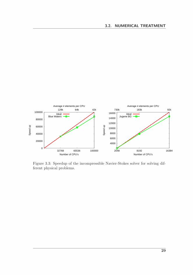
Fluid simulations have been tested on Blue Waters Supercomputer and Ju-gene Supercomputer with two viscous Navier-Stokes benchmarks, see Figure3.3.
28
3.2. NUMERICAL TREATMENT
0
20000
40000
60000
80000
100000
32768 65536 100000
129k 64k 42k
Spe
ed u
p
Number of CPU’s
Average # elements per CPU
IdealBlue Waters
4000
6000
8000
10000
12000
14000
16000
2048 8192 16384
730k 183k 92k
Spe
ed u
p
Number of CPU’s
Average # elements per CPU
IdealJugene BG
Figure 3.3: Speedup of the incompressible Navier-Stokes solver for solving dif-ferent physical problems.
29
4Rigid Body
In this chapter, once the Newton-Euler equations are introduced, we will explainthe numerical scheme that models the movement of a rigid solid given the forcesexerted on the body.
4.1 The Newton-Euler equations
The position of an arbitrary point inside a rigid body at a given time t can bedefined as
p(t) = x(t) + r(t), (4.1)
where x(t) is the position of the center of mass of the body and r(t) is theposition of p(t) relative to x(t). Considering that
r(t) = R(t) · r0,
where R(t) is the rotation of the body about x(t) and r0 is the initial positionof p(t) relative to x(t), Equation (4.1) can be rewritten as
p(t) = x(t) +R(t) · r0.
Taking into account that the rotation matrices are orthogonal, the velocityof p(t) can be expressed as
p(t) = x(t) + R(t) · r0
= v(t) + R(t) ·RT (t) · r(t),
where v(t) is the linear velocity of the body. The product R(t) ·RT (t) definesan antisymmetric tensor:
W (t) := R(t) ·RT (t) =
0 −ω3(t) ω2(t)ω3(t) 0 −ω1(t)−ω2(t) ω1(t) 0
, (4.2)
where ω1(t), ω2(t) and ω3(t) are the components of the angular velocity vectorω(t) of the body. The tensor W (t) is called the angular velocity tensor.
31
CHAPTER 4. RIGID BODY
The linear acceleration a(t) and angular acceleration α(t) of the body arerelated with the input force fF (t) and input torque τF (t) by the Newton-Eulerequations:
fF (t) = ma(t) (4.3)
and
τF (t) = I(t) ·α(t) + ω(t)× (I(t) · ω(t)), (4.4)
where m is the total mass of the body and I(t) is the inertia tensor. Byintegrating in time the Equations (4.3) and (4.4), the velocity and the positionof the rigid body can be determined.
4.2 The Newton-Euler discretization
Assume we know the force fn+1F and torque τn+1
F , exerted by the fluid, at thecurrent time step tn+1. Both will be approximated as described in Chapter 6.Then, the linear acceleration is easily computed by dividing the current forceexerted on a rigid body by the total mass of the body
an+1 =fn+1F
m.
The superscript n+ 1 refers to the current values of the simulation. The linearvelocity and linear displacement of the center of mass can be determined usingthe Newmark scheme as method of numerical integration. Given the time step∆t of simulation, the Newmark method states that the current linear velocityis equal to
vn+1 = vn +∆t(1− γ)an +∆tγan+1
and the current linear displacement is
xn+1 = xn +∆tvn +∆t2(1/2− β)an +∆t2βan+1,
where γ and β are specified coefficients of the integration method, and thesuperscript n refers to the values from the previous time step of the simulation.The coefficients γ and β are deeply studied in [41].
The angular velocity vector can also be computed using Newmark as methodof numerical integration:
ωn+1 = ωn +∆t(1− γ)αn +∆tγαn+1.
Nevertheless, the implementation of an iterative method is necessary in orderto obtain a good approximation of the solution of the nonlinear ordinary differ-ential Equation (4.4), the Euler rotation equation.
32
4.3. ALGORITHM OF THE EULER ROTATION EQUATION
4.3 Algorithm of the Euler rotation equation
The rotation of the body around its center of mass can be computed using therelation from Equation (4.2) as shown below:
Rn+1 = Rn +∆tW n ·Rn, (4.5)
where W n is the angular velocity tensor obtained from the previous time step.Then, the current components of W (t) are obtained by solving the Euler rota-tion equation. Thus, the current angular acceleration is equal to
αn+1 = (I−1)n ·[
τn+1F − ωn × (In · ωn)
]
,
and the angular velocity vector using Newmark as method of numerical inte-gration is
ωn+1 = ωn +∆t(1− γ)αn +∆tγαn+1.
Note that the components of the angular velocity tensor W (t) can be obtainedfrom the angular velocity vector ω(t).
Note also that the inertia tensor is time dependent, so it is necessary torecalculate their values at each time step. In order to avoid this expensive task,the following relation can be used:
I(t) = R(t) · J ·RT (t),
where J is the initial inertia tensor of the body. This tensor is a symmetrictensor and is defined by
I =
∫
ΩS
ρS (p · pId − p⊗ p) dΩS , (4.6)
where ΩS is the body domain, ρS is the body density, p defines the position of apoint in the body, Id is the identity tensor, and ⊗ represent the tensor product.
In the current numerical implementation, bodies are described by theirboundaries ΓS (boundary mesh.) It is therefore convenient to re-express theinitial inertia tensor of the body as an integral over its volume into an integralover its surface using the divergence/Gauss theorem, see [42] to a fast compu-tation of other body properties. Then, from Equation (4.6), we have that for
33
CHAPTER 4. RIGID BODY
each component of the inertia tensor I:
I11 =1
3ρS
∫
ΓS
p32n2 + p33n3 dΓS ,
I22 =1
3ρS
∫
ΓS
p31n1 + p33n3 dΓS ,
I33 =1
3ρS
∫
ΓS
p31n1 + p32n2 dΓS ,
I12 =1
4ρS
∫
ΓS
−p21p2n1 − p1p22n2 dΓS ,
I13 =1
4ρS
∫
ΓS
−p21p3n1 − p1p23n3 dΓS , and
I23 =1
4ρS
∫
ΓS
−p22p3n2 − p2p23n3 dΓS ,
where n1, n2, and n3 are the components of the exterior normal of the body inp.
Now, although the rotation matrix can be computed from (4.5), it is highlyrecommended to implement an iterative method to improve the approximatesolution of this non-linear system of equations. An alternative algorithm isdescribed below:
Initialize values: (·)i,n+1 = (·)n.Iterate while ǫ be higher than a given tolerance.
The superscript i+1 refers to the values of the current iteration, the superscripti to the values of the previous iteration, ǫ is a norm for the angular velocityvector, and (·) represent all the angular variables.
Numerical errors will appear in the coefficients of R(t) so that the rotationmatrix will no longer be precisely an orthogonal matrix. For this reason, ateach iteration it is necessary to reorthogonalize R(t), see [43]. To avoid thisproblem, unit quaternions can be used to represent rotations. However, it isimportant that the quaternions remain normalized at each iteration. A deeperdescription of quaternions and general implementation aspects can be found in[44].
34
4.3. ALGORITHM OF THE EULER ROTATION EQUATION
To finish, let us summarize the necessary steps to update the the position ofthe bodies (the coordinates of their boundary meshes.) Then, given the forceand torque exerted on a body, do:
• Determine the current linear displacement xi+1 using Newmark as methodof numerical integration.
• Determine the current rotation matrix Ri+1 using the iterative algorithmdescribed above.
• Finally, update the position p of each node that defines the boundarymesh of the body using the relation
p = xi+1 +Ri+1 · r0,
where r0 is the initial position of p relative to the center of mass of thebody.
35
5Rigid Body Interaction
In a simulation of a dynamic rigid body system we deal with multiple prob-lems. First, we have to determine the motion of particles due to external forces.Then, when the particles are in movement, we have to prevent interpenetrationbetween them and solve possible collisions when the bodies are in contact. Thesimulation framework of dynamic rigid bodies is well-known and tries to solvethe problems mentioned above. In this context, we will present the algorithmsto describe and solve the collision between bodies.
5.1 General Framework
The geometrical description of all the rigid bodies consists mainly of an STLfile describing the outer boundaries of the bodies. Note that a priori, only oneSTL description is necessary for each type of bodies.
For the sake of simplicity, we will consider the bodies as convex polyhedra.For non-convex bodies a convex decomposition is required.
In our simulation, we are able to solve the interaction between a lot of bodieswith different shapes. For this reason, a collision detection module, where thetime of collision is estimated, is necessary to avoid a situation where we need todo a lot of corrections to fix penetration between bodies. Also, we have to solvepossible collisions when the bodies are in contact. The simulation framework ofdynamic rigid bodies, see [32, 45, 46], solves all these problems in the followingconsecutive stages:
1. Collision Detection.
2. Rigid Body Motion.
3. Collision Response
Now, we will explain how to implement the first and the last stages mentionedabove. The rigid body motion was already described in Chapter 4.
5.1.1 Collision detection
Until now we determine the motion of bodies without considering collisions. Inthis context, the penetrations between bodies are not detected. To avoid thisunrealistic situation, we can proceed as described below:
1. We estimate a time of contact between bodies.
2. Then, we move the bodies freely until the estimated time is reached.
37
CHAPTER 5. RIGID BODY INTERACTION
To ensure not missing any collision we implemented a dynamic collision detec-
tion algorithm. In Figure 5.1 we see an example of a missing collision. Noticethat no penetration was detected between the two consecutive time steps t0 andt1. The algorithm we use to estimate the time of collision is detailed in [47].
t1 :
t0 :
Figure 5.1: Missing collision.
Let us briefly explain the idea. Consider two convex polyhedra A and B, thendetermine:
• The closest points between the bodies: pA on body A and pB on body B.
• The direction d = pA − pB .
• The minimum distance between bodies d = ‖d‖.
• The normalized direction d = d/d .
In Figure 5.2 we see two convex bodies A and B and their closest points. Next,if the last time step reached is t0, we define:
• DA(t) as an upper bound for the distance traveled by any point in A along−d in the time interval [t0, t].
• DB(t) as an upper bound for the distance traveled by any point in B alongd in the same time interval.
A collision occurs at time t = tc between the two convex bodies A and B if
DA(tc) +DB(tc) ≥ d.
This result is derived from the fact that the bodies are convex. Now, considerthe total acceleration of any point in the body:
atotal(t) = a(t) +α(t)× r(t),
38
5.1. GENERAL FRAMEWORK
BApB
pA d
Figure 5.2: Closest points between the bodies A and B.
where r is the position from the center of mass to the point. The accelerationof an arbitrary point in the direction of d is
atotal(t) · d = a(t) · d+ (α(t)× r(t)) · d,
and fulfillsatotal(t) · d ≤ a(t) · d+ αmaxrmax,
where rmax is the maximum distance of any point in the body from the center ofmass and αmax is the maximum angular acceleration in the time interval [t0, tc].Integrating twice over time the function on the right side of this inequality, asuitable expression for DA(t) and DB(t) is obtained. Thus, if we also considerthe inequality (5.1.1), we obtain an estimated value for the time of collision.
5.1.2 Collision response
Once the bodies reach the time of collision estimated by the collision detection,we need to identify the bodies in contact and, when it is necessary, calculatenew forces in order to avoid interpenetrations. These tasks are carried out bythe collision response.
We use an impulse-based method for computing the contact forces. Animpulse force is defined as
JS = lim∆t→0
∫ tc+∆t
tc
fdt,
where tc is the time of collision and ∆t is the period of time of collision. Animpulse produces an instantaneous change in the velocity of a body.
For frictionless bodies, the direction of the impulse is determined by the typeof contact. For the typical face-vertex contact, the direction of the impulse is
39
CHAPTER 5. RIGID BODY INTERACTION
the unit exterior normal of the face of contact. For edge-edge contact it is theunitized cross-product of the edge directions. Thus, we can express the impulseas
JS = jn(tc),
where j is the impulse magnitude and n(tc) is the unit collision vector.Now, consider two polyhedra bodies A and B in contact and suppose that
the unit collision vector n(tc) is in body B, see Figure 5.3. The relative velocityof these two bodies is defined as
vrel = n ·(
(v−A + ω−
A × rA)− (v−B + ω−
B × rB))
.
If the relative velocity vrel is positive, the bodies are moving apart. But if vrelis negative, the bodies are moving closer together. Then, an impulse force isnecessary to change the velocity of the bodies in order to avoid interpenetration.
Take into account that the magnitude j of the impulse is still undetermined.Then, to obtain an expression for j we have to consider the empirical law forfrictionless collisions which relates the velocities of the bodies before and afterthe collision. The empirical law for frictionless collisions states that
n(tc) ·(
u+A(tc)− u+
B(tc))
= −cn(tc) ·(
u−A(tc)− u−
B(tc))
, (5.1)
where uA is the total velocity of body A, uB is the total velocity of body B, cis the restitution coefficient, the superscript + indicates the quantities after thecollision and the superscript − the quantities before the collision. When c = 1,the collision is perfectly elastic. If c = 0 the collision is perfectly inelastic. For acollision that is perfectly elastic, the momentum and kinetic energy is conservedby the empirical law for frictionless collisions.
BA n
Figure 5.3: Contact between two bodies.
40
5.2. GEOMETRIC TOOLS ALGORITHMS
On the other hand, the linear and angular velocities in body A, after thecollision, are related with the previous linear and angular velocities through animpulse by equations
v+A(tc) = v−
A(tc) +jn(tc)
mA
(5.2)
and
ω+A(tc) = ω−
A(tc) + I−1A (tc) (rA(tc)× jn(tc)) , (5.3)
where vA is the linear velocity of body A, wA is the angular velocity of A, mA
is the mass of A, I−1A is the inverse of inertia tensor of A, and rA is a vector
defined from the contact point to the center of gravity of A. For body B wemust consider the opposite impulse −JS .
Now, considering the total velocity of body A after collision:
u+A(tc) = v+
A(tc) + ω+A(tc)× rA(tc)),
by Equations (5.2) and (5.3) we obtain that
u+A(tc) = v−
A(tc) +jn(tc)
mA
+(
ω−A(tc) + I−1
A (tc) (rA(tc)× jn(tc)))
× rA(tc).(5.4)
A similar expression can be obtained for body B considering the opposite im-pulse −JS .
Finally, the magnitude j of the impulse can be obtained replacing the equa-tion (5.4) for body A in Equation (5.1), the law for frictionless contacts, andfor body B with the opposite impulse −JS . Thus, the magnitude j is equal to
j =−(1 + c)n ·
(
(v−A + ω−
A × rA)− (v−B + ω−
B × rB))
1mA
+ 1mB
+ n ·(
I−1A (rA × n)
)
× rA + n ·(
I−1B (rB × n)
)
× rB.
An expression for j is also obtained in [32].
5.2 Geometric tools algorithms
Important issues in the collision detection, the collision response, and the fluidand particles interactions are related to the implementation of efficient algo-rithms to search the minimum distance between a pair of particles or to de-termine if a node in the mesh is contained inside a particle. These searchescan affect the performance of the whole system in a negative way: the time ofsimulation can grow considerably. To reduce the number of computations ofthis expensive task, it is necessary to implement different kind of structures tooptimize these searches.
41
CHAPTER 5. RIGID BODY INTERACTION
5.2.1 Skd-Trees
The skd-trees are binary trees. These structures are bounding volume hierar-chies. Each node of these binary trees is a bounding volume for a subset offaces of a particle. In particular, a skd-tree allow us to find the shortest dis-tance between a point and a surface mesh in an efficient way. The details ofimplementation for building these structures for a particle are described in [48]and outlined below:
1. Create a new node, the root node, see Figure 5.4.
2. Link all the faces of the particle with the root node.
3. Do for each newly created node whenever it has more than one face:
• Determine the boundary box that contains all the faces linked to thecurrent node.
• Store the boundary box in the current node.
• Find the largest dimension of the boundary box, let us denote as d.
• Distribute the faces into two distinct sets. If n is the current numberof faces, each set will have n/2 number of elements. The centroids ofthe boundary boxes of the faces in the first set will have the smallestvalues on the d coordinate. The second set will have the biggest ones.
• Unlink the faces for the current node.
• Create two new nodes, the child nodes of the current node.
• Link the faces in the first set with the first child node.
• Link the faces in the second set with the second child node.
The skd-tree construction for a particle is schematized in Figure 5.4. The thinred line indicates that the faces are not linked to the node and their informationis not available. However, the information of the boundary box that containsthe faces is still available. Only the leaf nodes, the nodes that do not have anychildren, have a face linked with them.
In [48] it is also described how to use the skd-trees to find the shortestdistance between a point and a particle. The idea is to minimize an upper boundfor the distance between the point and the particle while we are traversing thebinary tree from the root node. We will denote this upper bound as dis. Thealgorithm is summarized below:
1. Determine the maximum distance between the point and the boundarybox of the root node. Let us define this value as dis.
2. Traverse the binary tree from the root node in pre-order and perform thefollowing operations:
• Determine the minimum distance between the point and the bound-ary box of the current node. Let us define this value as min.
42
5.2. GEOMETRIC TOOLS ALGORITHMS
child nodes
child nodes
leaf nodes
87
4
2
6 5
6
87
6
1
1
7
7
65
3
53
4root node
345
1
1
438
82
2
2
body faces
body boundary box
Figure 5.4: The skd-tree construction for a particle. The surface mesh of thebody has 8 edges.
• If min is smaller than dis then:
– If the current node is a leaf, a node that does not have anychildren, then there is one face identifier linked to the node.Save it in a candidate list.
– If the current node is not a leaf then determine the maximumdistance between the point and the boundary box of the currentnode. Let us define this value as max. If max < dis thendis = max.
• Else, do not traverse the subtree below the current node.
3. Find the distances between the point and all the faces associated in thecandidate list. Choose the smallest one.
Improvement in Skd-tree searching
A simple modification is implemented when we use the skd-trees in order toobtain a better performance in the simulation. In practice, we obtain betterresults if we first visit the nodes whose boundary boxes are closest to the pointwhen we traverse the tree from the root node. The idea is described below:
1. Determine the maximum distance between the point and the boundarybox of the root node. Let us define this value as dis.
43
CHAPTER 5. RIGID BODY INTERACTION
2. Traverse the binary tree from the root node in pre-order and perform thefollowing operations:
• Determine the minimum distance between the point and the bound-ary box of the current node. Let us define this value as min.
• If min is smaller than dis then:
– If the current node is a leaf, a node that does not have anychildren, then there is one face linked to the node. Find thedistance between the point and this face and save it as new dis.If new dis < dis then dis = new dis.
– If the current node is not a leaf then sort their two child nodessuch that we visit first the child node whose boundary box isclosest to the point.
• Else, do not traverse the subtree below the current node.
3. dis has the minimum distance between the point and the particle.
These structures was used in different applications [1, 3, 5, 6].
5.2.2 Closest points between particles
In order to determine the time of collision between two particles we first haveto find the closest points between them. An algorithm to calculate the distancebetween two convex bodies is described in [49] and it is summarized below.
• Find the minimum distance dA between the nodes of A and the particleB.
• Find the minimum distance dB between the nodes of B and the particleA.
• Find the minimum distance dE between the edges of A and the edges ofB.
• Choose the shortest distance between dA, dB and dE .
All these tasks can be carried out using skd-trees to obtain better computationaltimes of execution.
5.2.3 Bucket sort
The idea is to subdivide the domain along each coordinate to obtain buckets orboxes with the same size in all the coordinates. This grid may have differentnumbers of boxes in each direction. The boxes will contain elements that areinside or intersect with them. The construction details are shown in [50].
By incorporating this kind of structure in the code, we will able to reducethe size of the search space when we need to carry out some local operationswith the elements contained in the boxes.
44
5.2. GEOMETRIC TOOLS ALGORITHMS
In particular, this structure is used to store the nodes of the mesh in differentboxes. Thus, in order to determine the nodes that are inside a body at eachtime step of the simulation, we only need to check the nodes inside the boxesthat intersect with the boundary box of the body.
Consider the elements and nodes of the mesh shown in Figure 5.5, repre-sented by small black squares and small circles respectively. The body and itsrespective boundary box are represented by a big red circle and a big red square.The big black squares represent a bucket sort structure, where the nodes of themesh are stored. Then, in order to find the nodes inside the body, the programhas only to consider the nodes in the mesh inside the boxes that intersect withthe boundary box of body, the white circles in Figure 5.5.
checked node
unchecked node
Figure 5.5: Bucket sort structure. In order to find the nodes inside the body,the program has only to consider the nodes represented by white circles, thenodes in the mesh inside the boxes that intersect with the boundary box ofbody.
45
6Rigid body and fluid interaction
In this chapter we describe in detail the mathematical and numerical models tosolve the interaction between a fluid and a rigid body. The solid is taken intoaccount on the fluid by imposing the body surface velocity on the fluid as aDirichlet boundary condition and the motion of the body is determined by theforce and torque that the fluid exerts on its surface.
The numerical simulation of a fluid and its interaction with rigid bodiesrequires the implementation of many different algorithms. In order to presentthese algorithms in a organized manner we will first describe a general algorithmto solve the fluid and rigid body interaction. Then, we will describe in detaileach part of the algorithm. These algorithms will be described considering aparallel context.
6.1 Framework of an embedded boundary mesh method
Let ΩF and ΩS be the fluid and solid domain, where ΩS is the union of all thedomains associated to the rigid bodies in the problem. Then, in an embeddedboundary mesh method, at the beginning, ΩF ∪ ΩS is discretized without anyparticular regard to the rigid bodies. The movements of the boundaries de-scribes the movements of the solids inside the fluid. Then, at each time step ofthe simulation, the nodes and elements that are considered as part of the solidswill be excluded from the assembly process. Finally, the solids are taken intoaccount on the fluid by imposing the body velocity on the fluid as a Dirichletboundary condition in an interpolated way.
In particular, at each time step of the simulation, the program identifies theelements in E whose volumes of intersection with the rigid body domain are bigenough to consider them as part of the solid, that is, elements that belong to theset of hole elements Ehol, see Figure 6.1. They are then excluded from the finiteelement assembly process. Let ΓS,h be the internal boundary mesh generatedin the fluid mesh once the hole elements have been excluded. In Figure 6.1 thebold black line represents ΓS,h. Inside this closed line one can find the holeelements represented by gray squares. In a embedded boundary mesh method,the velocity of the rigid solid is imposed on the nodes that define ΓS,h. Letthis set be the set of fringe nodes: Nfri. The set Nfri allow us to define otherimportant sets of nodes: the set of free Nfre and the set of hole nodes Nhol.The set of free nodes belongs to the discretized fluid domain and the set of holenodes belongs to the discretized solid domain, see Figure 6.2.
Some of the implementation details of the embedded mesh boundary meth-ods described next in this work was published previously in [1, 6].
47
CHAPTER 6. RIGID BODY AND FLUID INTERACTION
Ehol
ΓSh
Figure 6.1: Hole elements and ΓS,h schematization.
∈ N f ri
∈ N f re
∈ Nhol
Figure 6.2: Fringe, free and holes nodes.
48
6.2. FLUID AND RIGID BODY INTERACTION ALGORITHM
6.2 Fluid and rigid body interaction algorithm
The numerical schemes to solve the Navier-Stokes (NS) and the Newton-Euler(NE) equations need information from each other to account for the interaction.In order to close the problem, one is left with the variables involved in thecoupling between the fluid and the rigid body problems. On the one hand, thevariables that the fluid receives from the rigid body are enumerated below:
• The linear velocity vn+1 of the rigid body from Equation (4.3).
• The angular velocity wn+1 of the rigid body taken from Equation (4.4).
• The definition of the boundary mesh Γn+1S,h once the program excludes the
hole elements from the fluid discretization at the current time step n+ 1.
• The total velocity un+1S to be imposed on Γn+1
S,h . That is, the velocity
of the set of fringe nodes Nn+1fri to approximate the rigid body boundary
velocity.
On the other hand, the set of variables that the solid requires from the fluidproblem is enumerated below:
• The force fn+1F that the fluid exerts on the rigid solid.
• The torque τn+1F that the fluid exerts on the rigid solid.
Taking into account all the coupling variables described above, a new cou-pling strategy is briefly described in Algorithm 5.
Algorithm 5 NS-NE Coupling strategy
Initialize the variablesrepeat
1. Determine the time step ∆t, see Subsection 6.2.4.2. Solve NE equations to obtain vn+1 and wn+1, see Chapter 4.3. Define Γn+1
S,h , which implies to determine Nn+1fri , see Subsection 6.2.1.
4. Determine un and unmsh applying the FMALE method, see Subsection
6.2.3.5. Embedded approaches. Impose un+1
S on Nn+1fri , see Subsection 6.2.2.
6. Solve the NS equations to obtain un+1 and pn+1, see Chapter 3.7. Determine fn+1
F and τn+1F from un+1 and pn+1, see Subsection 6.2.5.
until the time of simulation is reached
Note that the NS-NE system is a two-way coupled problem. Therefore,Algorithm 5 consists of a staggered approximation of the coupled solution ateach time step, as no coupling loop has been introduced and variables Γn+1
S ,un+1S , fn+1
F and τn+1F are approximations of the actual values at time step
n + 1. We thus expect the accuracy of the scheme to depend not only on
49
CHAPTER 6. RIGID BODY AND FLUID INTERACTION
S T
inside node
near node
∈ NSi f a,own
∈ NTi f a,own
Figure 6.3: Near and inside nodes.
the way the set of coupling variables is defined but also on the time step ∆t.Another important issue is the so-called added mass effect [51], which may causeinstabilities in many cases. In order to circumvent this problem, it is importantto make sure that the ratio between fluid and solid densities is not too closeto the unity [52]. In the numerical experiments presented in this thesis, theseratios are rather small than the unity and we have not observed any instability.However, it must be said that subiterations at each time step could be used toachieve a strong coupling, increasing the computational cost, but without theneed of significant effort in a parallel implementation.
Let us now describe in detail each step of Algorithm 5.
6.2.1 Algorithms to define an approximated body bound-
ary Γn+1
S,h
Fringe nodes identification algorithm
The idea is simple, but the implementation, specially in a parallel context, issomehow complicated.
First, for each subdomain, we have to identify the nodes inside the body,and then the nodes outside and near the body, see Figure 6.3.
It is important to remark that the round-off errors of the geometric opera-tions such as the projection of a node on the solid and its minimum distance cancause that a node n located at the interface between subdomains be consideredas part of the solid for a subdomain and as part of the fluid for another one.In order to avoid these errors, each subdomain S will be the only responsiblefor identifying the set of inside and near nodes considering the subset of nodesN S
int ∪NSifa,own as illustrated in Figure 6.4. Thanks to the definition of the set
of own interface nodes N Sifa,own for an arbitrary subdomain S, see Chapter 2,
the program will be able to consider all the nodes in the mesh without consider
50
6.2. FLUID AND RIGID BODY INTERACTION ALGORITHM
|NS ∪ NShal|
...
|NS|+ 1
|NS|
...
|NSint ∪ NS
ifa,own|+ 1
|NSint ∪ NS
ifa,own|
...
|NSint|+ 1
|NSint|
...
2
1
computed bythe adjacents subdomains of S
computed by S(interior and own interface nodes of S)
Figure 6.4: Array of data related with the set of nodes of S. The gray zonerepresents the nodes take into account by S.
the same node twice in a parallel execution.
Precises definitions of the set of inside and the set near nodes are carriedout by Algorithms 6 and 7 respectively. As mentioned above, each subdomainS identify the set of inside and the set of near nodes considering only the setNS
int ∪ NSifa,own. Then, the new data is exchanged between the subdomains at
the end of each algorithm using the algorithms of exchange INE and HNEdefined in Subsections 2.5.1 and 2.5.2 respectively.
In Algorithm 6, the bin search uses the bucket sort structure explained inSubsection 5.2.3. This structure allows us to reduce the size of the search fornodes in N S
int ∪NSifa,own that are inside the body considering only the nodes in
the boxes of the bucket sort structure that intersect with the boundary box ofthe body.
In Algorithm 7 the idea, as illustrated in Figure 6.3, is to obtain a set offringe nodes closer to the rigid body surface mesh.
Then, considering a node n ∈ N S ∪ NShal, for an index iS = indexS(n) we
have that
inside(iS) =
1 when n is inside the body
0 when n is outside the body
after the execution of Algorithm 6, and
near(iS) =
1 when n is near the body
0 when n is not near the body
51
CHAPTER 6. RIGID BODY AND FLUID INTERACTION
Algorithm 6 Inside nodes identification algorithm for an arbitrary subdomainS
Require: A numeric array inside with length |N S ∪NShal|
Ensure: A modified array insideInitialize inside(1 : |N S ∪ N S
hal|)← 0Bin search. Select a reduced candidate list of nodes in NS
int ∪NSifa,own using
the bucket sort structure, see Subsection 5.2.3.for each node n ∈ NS
int ∪NSifa,own in the previous list do
Skd-tree search. Efficiently determine if n is inside the bodyif n is inside then
iS = indexS(n)inside(iS) = 1
end ifend forcall INE(inside(1 : |N S |)), see Algorithm 1.call HNE(inside(1 : |N S ∪ N S
hal|)), see algorithm 2
Algorithm 7 Near nodes identification algorithm for an arbitrary subdomainS
Require: A numeric array near with length |N S ∪NShal|
Ensure: A modified array nearInitialize near(1 : |N S ∪NS
hal|)← 0for each node n ∈ N S
int ∪ NSifa,own outside the body do
for each node m ∈ Cnod(n) inside the body doif n is closer to the surface mesh than m then
iS = indexS(n)near(iS) = 1
end ifend for
end forcall INE(near(1 : |N S |)), see Algorithm 1call HNE(near(1 : |N S ∪ N S
hal|)), see Algorithm 2
52
6.2. FLUID AND RIGID BODY INTERACTION ALGORITHM
after the execution of Algorithm 7.
Finally, once the Algorithms 6 and 7 have been executed, we can determinethe fringe nodes as described in Algorithm 8. By definition, a fringe node n hasat least one free and hole node in its node connectivity Cnod(n). That is, n isan inside or near node with at least one node outside and not near the body inCnod(n), a node at the interface between a solid and the fluid.
Algorithm 8 Fringe nodes identification algorithm for an arbitrary subdomainS
Require: A numeric array fringe with length |N S ∪NShal|
Ensure: A modified array fringeInitialize fringe(1 : |N S ∪ N S
hal|)← 0for each node n ∈ NS inside or near the body do
if there is at least one node outside and not near the body in Cnod(n)then
iS = indexS(n)fringe(iS) = 1
end ifend forcall HNE(fringe(1 : |N S ∪ N S
hal|)), see Algorithm 2
As before, considering a node n ∈ N S ∪NShal, for an index iS = indexS(n)
we have that
fringe(iS) =
1 when n is a fringe node
0 when n is not a fringe node
after the execution of Algorithm 8.
Free and hole nodes identification algorithm
The set of free Nfre and hole nodes Nhol are defined as the set of nodes inthe mesh that are outside and inside the body respectively, excluding the set offringe nodes Nfri.
Hole and free elements Identification algorithm
The elements that will be considered as a part of the solid, the set of holeelements Ehol, see Figure 6.1, can be easily identified from the set of fringe,free and hole nodes. The process is described in Algorithm 9 for an arbitrarysubdomain S. As mentioned in this chapter, the set of hole elements Ehol willbe excluded from the finite element assembly process.
Finally, the set of free elements is defined as Efre = E\Ehol.
53
CHAPTER 6. RIGID BODY AND FLUID INTERACTION
Algorithm 9 Solid elements identification algorithm for an arbitrary subdo-main S
for each element e ∈ ES ∪ EShal doif all the nodes n ∈ e belong to Nfri or Nhol then
e will be considered as part of the solid, that means e belongs to Ehol.end if
end for
6.2.2 Embedded approaches
In our implementation, two approaches that allow us to impose the velocity ofthe rigid body on ΓS,h are considered: an updated body fitted and a non bodyfitted strategies. The first approach implements a local r-adaptivity algorithmthat moves the nodes in N close to the rigid body surface in order to adapt theirposition to that of the body surface mesh. The second approach implements ahigh order kriging interpolation to impose the velocity of the body on the nodesin N close to the rigid body surface.
Updated body fitted method (UBF)
The updated body fitted approach implements a local r-adaptivity algorithmthat moves the set of fringe nodes Nfri incrementally until the body surfacemesh is reached. Then, the program directly imposes the velocity of the rigidbody in each fringe node nfri equation as:
ufri = uS(xfri),
where ufri is the fringe node velocity, xfri is the spatial coordinates of thefringe node and uS(xfri) is the velocity of the solid at xfri.
Actually, in our implementation, the algorithm that defines the movementof the nodes of the fluid mesh involves several sets of nodes besides the set offringe nodes. The reason is to avoid distorted or inverted elements.
In this context, the algorithm also defines the movement of a group of subsetsof the set of free nodes that have a close connectivity with the set of fringe nodes.In order to elucidate what we mean by ‘close connectivity’, let us introduce somedefinitions. Define the subset
N 1fre =
⋃
n∈Nfri
Cnod(n) \(Nfri ∪ Nhol)
as the set of free nodes at level 1, see Figure 6.5. In an analogous way, a secondsubset
N 2fre =
⋃
n∈N 1
fre
Cnod(n)∖(
N 1fre ∪ Nfri
)
54
6.2. FLUID AND RIGID BODY INTERACTION ALGORITHM
S T
n ∈ N2f re
n ∈ N1f re
n ∈ N f ri
n ∈ NSi f a,own
n ∈ NTi f a,own
Figure 6.5: Sets of free nodes at different levels. The red concentric circlesrepresent the set Nfri. The sets N 1
fre and N 2fre surround the set of fringe
nodes.
will be called the set of free nodes at level 2, see Figure 6.5. In general, thesubset
N lfre =
⋃
n∈N l−1
fre
Cnod(n)∖(
N l−1fre ∪ N
l−2fre
)
defines the set of free nodes at level l ∈ N\0, 1, 2. Evidently, the smaller thevalue of l, the closer the connectivity with the set of fringe nodes.
The movement of the nodes of the fluid mesh is incremental and finisheswhen the set of fringe nodes reaches the body surface mesh. In particular, foreach increment in the movement of the set of fringe nodes, there are several
increments in the movement of the free nodes that belong to the set⋃
l≤level
N lfre
for a given value of level. The flow of the whole algorithm is illustrated inFigure 6.6.
In particular, the movement of the free nodes is defined by a Laplacian-likesmoothing technique similar to that described in [53, 54]. In these references,a node n is relocated in the centroid c of the nodes directly connected with n:the set of nodes Cnod(n), as described in Algorithm 10. In our approach, weperform some treatment to the set Cnod(n) so that the region defined by thesenodes be convex.
On the other hand, the movement of the set of fringe nodes is more complex.The movement for a fringe node n is illustrated in Figure 6.7 and performed asindicated below:
• Determine the centroid c of the set Cnod(n)∩Nfri, see Figure 6.7(Middle.)
55
CHAPTER 6. RIGID BODY AND FLUID INTERACTION
Start
increasep f ri (until 1.0)
for each noden ∈ N f ri do:1. determine the centroidc of Cnod(n) ∩N f ri
2. determine the projectionp of c on ΓS ,h
3. moven towardsp in a proportionp f ri
l ← l + 1
increasep f re (until 1.0)
for each noden ∈ N lf re do:
1. determine the centroidc of Cnod(n)2. moven towardsc in a proportionp f re
Hasn ∈ N lf re reachedc(n)?
Is l > level, wherelevel ∈ N\0
Hasn ∈ N f ri reachedΓS ,h?
End
p f ri ← 0
l← 0
p f re ← 0
yes
yes
yes
no
no
no
Figure 6.6: A scheme of the algorithm that defines the movement of nodes. Thebody surface mesh is represented as ΓS,h. The parameters pfri and pfre arethe proportions of the movement of the set of fringe and free nodes respectively.And the value c is the centroid defined by the set of nodes Cnod(n).
• Determine the point of projection p on the body surface mesh of c, seeFigure 6.7(Middle.)
• Move n towards p, see Figure 6.7(Bottom.)
A precise description of the movement of the set of fringe and the set of freenodes at a given level is described next considering a parallel context.
Parallel movement algorithm
Consider now a distributed memory parallelization environment. An incre-ment in the movement of the set of fringe nodes is described in Algorithm 11.And an increment in the movement of a set of free nodes at a given level isdescribed in Algorithm 12. In both algorithms, as before, only one subdomain
56
6.2. FLUID AND RIGID BODY INTERACTION ALGORITHM
ΓS ,hn
ΓS ,h
Cnod(n) ∩ N f ri
c
p
n
ΓS ,h
p
n
∈ E f re
∈ Ehol
∈ N f ri
∈ N f re
∈ Nhol
Figure 6.7: The movement of a fringe node n considering only one increment.(Middle) First, we have to determine the centroid c of the set of nodes Cnod(n)∩Nfri. (Bottom) Then, we move the node n towards the projection p of c on theboundary mesh.
defines the movement of an interface node The idea is illustrated in Figure 6.5.The subdomain S only moves the interface nodes inN S
ifa,own and the subdomain
T the interface nodes in N Tifa,own.
The whole movement is described in Algorithm 10 for a given number ofincrements and levels of the set of free nodes. From here, the Algorithms1 11and 12 are called.
Non body fitted embedded method (NBF)
The non body-fitted approach implements a high order kriging interpolationalgorithm. The idea is to impose the velocity of the body for each fringe nodenfri in an interpolating way. For this purpose, the program first has to considera convenient subset of the set of free nodes Nfre that have a close connectivitywith nfri; denote it as Nsel(nfri). Then, the program imposes the velocity of
57
CHAPTER 6. RIGID BODY AND FLUID INTERACTION
Algorithm 10 R-local adaptivity algorithm for an arbitrary subdomain S
Require:1. An array coordinates with the positions of the nodes in N S ∪ N S
hal
2. A value for levelEnsure: A modified array coordinates
proportion fringe← 0repeat
increase proportion fringecallMOVE FRINGES(coordinates, proportion fringe), see Algorithm
11l← 0repeat
l = l + 1proportion free← 0repeat
increase proportion freecall MOVE FREES(coordinates, l, proportion free), see Algo-
rithm 12until proportion free = 1
until l ≥ leveluntil proportion fringe = 1
Algorithm 11 Fringe nodes movement algorithm MOVE FRINGES for anarbitrary subdomain S
Require:1. An array coordinates with the positions of the nodes in N S ∪ N S
hal
2. A value for proportionEnsure: A modified array coordinates
Initialize new coordinates(1 : N S ∪ N Shal)← 0
for n ∈ Nfri ∩ (NSint ∪NS
ifa,own) doDetermine the centroid c defined by Cnod(n) ∩ Nfri
Determine the projection p of c on ΓS,h
Determine the position in order to move n towards p in a proportion equalto proportion and save it in position
iS = indexS(n)new coordinates(iS) = position
end forcall INE(new coordinates(1 : |N S |)), see Algorithm 1call HNE(new coordinates(1 : |N S ∪ N S
hal|)), see Algorithm 2coordinates← new coordinates
58
6.2. FLUID AND RIGID BODY INTERACTION ALGORITHM
Algorithm 12 Free nodes movement algorithm MOVE FREES for an arbi-trary subdomain S
Require:1. An array coordinates with the positions of the nodes in N S ∪ N S
hal
2. A value for level3. A value for proportion
Ensure: A modified array coordinatesInitialize new coordinates(1 : N S ∪ N S
hal)← 0for n ∈ N level
fre ∩ (NSint ∪NS
ifa,own) doDetermine the centroid c defined by Cnod(n)Determine the position in order to move n towards c in a proportion equal
to proportion and save it in positioniS = indexS(n)new coordinates(iS) = position
end forcall INE(new coordinates(1 : |N S |)), see Algorithm 1call HNE(new coordinates(1 : |N S ∪ N S
hal|)), see Algorithm 2coordinates← new coordinates
the rigid body in the fringe node nfri equation as
Nfriufri +∑
ni∈Nsel(nfri)
Niui = uS(xS),
where ui is the velocity of free node ni, xS is the projection point of the fringenode on the surface mesh of the body, and uS(xS) is the velocity of the bodyat xS . Nfri and Ni are the interpolation coefficients determined by solving thematrix kriging system.
The whole algorithm can be divided into three consecutive main steps. Foreach fringe node n in Nfri do:
• The selection of a convenient subset of free nodes that has a close connec-tivity with n to perform the interpolation: Nsel(n) ⊂ Nfre.
• The assembly of the matrix of the kriging system to interpolate the bodysurface velocity. In particular, this velocity will correspond to the solidvelocity at the projection point p of n on the body surface. The positionsof the free nodes in Nsel(n) and p will be used in the assembly.
• The inversion of the matrix of the kriging system by using the LU decom-position method in order to obtain the interpolation coefficients Nfri andNi of Equation 6.2.2.
Parallel element and nodes selection
59
CHAPTER 6. RIGID BODY AND FLUID INTERACTION
The interpolation requires to previously select a subset of the set of free nodesNfre with a close connectivity with a fringe node n. The idea is schematized inFigure 6.8.
ΓS
ΓS
ΓS
n
Figure 6.8: Illustration of the selection algorithm. the gray square denotesesel(n). The red concentric circles denote members of the set of fringe nodes,and the black circles are the free nodes that belong to set Nsel(n).
Considering an arbitrary fringe node n, the definition of the set Nsel(n) canbe carried out in an algorithmic fashion as follows:
• Select a convenient element esel(n) containing n, that is n ∈ esel(n). InFigure 6.8, the gray square denotes esel(n).
• Then, let
Nsel(n) =⋃
m∈esel(n)
Cnod(m) ∩ Nfre
be the definition of the set of nodes used to perform the interpolation. InFigure 6.8, the black circles are free nodes that belong to set Nsel(n).
Algorithm 13 describes in detail the selection of nodes considering a parallelcontext. It can be divided into two parts. In the first part, each fringe node nstarts by selecting a convenient element esel(n). The idea is to select an elemente = ne
1, ne2, n
e3, ... with ne
1, ne2, n
e3, ... close to the boundary of the body.
As explained in Subsection 6.2.1, only one subdomain has to execute thegeometric operations for any arbitrary node located at the interface betweensubdomains in order to assure the coherency of the data. For this reason, anyarbitrary subdomain S will consider only its set of interior nodes NS
int and itsset of own interface nodes N S
ifa,own to select esel(n).At the end of the first part of the Algorithm 13 the data is exchanged between
the subdomains using the algorithms of exchange INE and HNE defined inSubsections 2.5.1 and 2.5.2 respectively.
In the second part, each fringe node n defines the set of nodes Nsel(n) toperform the interpolation taking into account esel(n).
60
6.2. FLUID AND RIGID BODY INTERACTION ALGORITHM
Algorithm 13 Selection nodes algorithm for an arbitrary subdomain S
⊲ Selection of the convenient element esel(n)Initialize element(1 : |N S ∪ N S
hal|)← 0for each node n ∈ Nfri ∩ (N S
int ∪ NSifa,own) do
for each element e ∈ Cele(n) (including EShal) do
if the distance from the centroid of e to n is the smallest one theniS ← indexS(n)element(iS)← the global id of e
end ifend for
end forcall INE(element(1 : |N S |)), algorithm 1call HNE(element(1 : |N S ∪ N S
hal|)), algorithm 2⊲ Selection of the set of nodes Nsel(n)
for each node n ∈ Nfri ∩ N S dofor each element e ∈ Cele(n) ∩ E
S) doiS ← indexS(n)if the global id of e is equal to element(iS) then
Select the set of nodes Nsel(n) =⋃
m∈esel(n)
Cnod(m) ∩ Nfre for n
end ifend for
end for
61
CHAPTER 6. RIGID BODY AND FLUID INTERACTION
Kriging interpolation algorithm
In particular, we use an approximation method known as the universal kriging.The concepts and implementation aspects are detailed in [55].
In the kriging approach, the unknown function is the sum of a mean valueµ(x) and an error term ǫ(x):
F (x) = µ(x) + ǫ(x),
where x is the position vector of the unknown function.The approximation function for F (x) is expressed as a linear combination
of the data F (xi)i=1,n:
f(x) =
n∑
i=1
Ni(x)F (xi).
The weights Ni are chosen to minimize the squared variance of the error ofprediction:
Var (F (x)− f(x))2= Var
(
F (x)−n∑
i=1
Ni(x)F (xi)
)2
,
subject to the unbiasedness condition. This condition states that the mean ofthe unknown function is equal to the mean of its approximation:
µ(x) =
n∑
i=1
Ni(x)µ(xi).
Our choice for the mean of the unknown function is a polynomial function.Some implementation aspects are taken from [56].
6.2.3 FMALE
As mentioned before, the proposed embedded boundary techniques identify aset of free nodes Nfre, a set of fringe nodes Nfri, and a set of hole nodes Nhol
at each time step of the simulation. Then, only the nodes in Nhol are excludedfrom the finite element assembly process. Now, consider the nodes inNfre∪Nfri
at the current time step tn+1 that were hole nodes at the previous time steptn. They are the new fluid nodes of the simulation at tn+1. These nodes weretherefore, for practical purposes, nonexistent at the previous time step. Then,one of the practical problems with these new fluid nodes consists in defining thevelocities at the previous time step tn, which are required by the Navier-Stokesequations to compute the time derivatives.
62
6.2. FLUID AND RIGID BODY INTERACTION ALGORITHM
This problem can be solved by considering a hidden motion of the meshfrom tn to tn+1, which can be explained and formulated in the framework ofthe FMALE method [57]. In this work, new characteristics are adopted insidethe FMALE implementation in order to improve the results obtained. Thesenew features are explained below. But first, it is important to know in detailhow the FMALE works.
We slightly reinterpret the FMALE algorithm described in [57] here. Itconsists of the following:
• Move the mesh at the current time step tn+1 such that all the new fluidnodes lie on the fluid domain at tn. This virtual time step being referredto as tn∗ .
• Then, interpolate the values of the previous velocity onto this new meshfrom the solution obtained at tn.
• Finally, compute a mesh velocity umsh to be included in Equation (3.1)in order to recover the original mesh at tn+1 from tn∗ and to account forthe mesh motion.
In order to illustrate the FMALE approach, let us consider the one-dimensionalexample shown in Figure 6.9. The dotted lines represent the solid body at tn,which moves to the right, and depicted with continuous lines at tn+1, see Figure6.9 (original mesh). At time tn, the fringe node is node n3 and at time tn+1 weend up with a new free node n4, and a new fringe node n5. The procedure isdescribed below:
• Prescribe a displacement for the new fringe node n5 such that at tn it fallsinto the fluid, and move it incrementally together with nodes n3 and n4.Nodes n1 and n2 are assumed to be sufficiently far to remain fixed. Theresulting new mesh at tn∗ is shown in Figure 6.9 (b).
• The values of the velocities for the moved nodes n3, n4 and n5 are theninterpolated from the solution obtained at time tn. This interpolation isrepresented by the vertical arrows between Figures 6.9(b) and 6.9(a).
• The mesh velocity is then computed from the positions obtained at timetn∗ to recover the positions of the nodes on the original mesh tn+1, Figures6.9(b) and 6.9(c) for nodes n3, n4 and n5. The nodal mesh velocity issimply ui
msh = (xn+1i − xn∗
i )/∆t. The mesh velocity is represented byhorizontal arrows.
A new virtual movement of the mesh inside the FMALE framework
The positions of the nodes at the previous virtual time step tn∗, as it is illus-trated in Figure 6.9(b), are determined by the r-local adaptivity Algorithm 10.
63
CHAPTER 6. RIGID BODY AND FLUID INTERACTION
original mesh:
ΓnS Γn+1
Sn1 n2 n3 n4 n5 n6
(a) timetn:n1 n2
xn4
xn5
xn6n3
(b) time tn∗ :u5
mshu4mshu3
msh
n1 n2 n3 n4 n5x
n6
(c) timetn+1:n1 n2 n3 n4 n5
xn6
Figure 6.9: Illustration of the FMALE framework. The dotted lines representthe body surface mesh at the previous time step tn and the continuous lines rep-resent the body surface mesh at the current time step tn+1. The red concentriccircles denote members of the set of fringe nodes, black circles members of theset of free nodes, and crosses members of the set of hole nodes. The plots (a)and (c) represent the fluid mesh in two consecutive time steps after remeshing.
Considering the mesh at the current time step tn+1, the idea is to incrementallymove the set of fringe nodes Nfri and a subset of the set of free nodes untilNfri reaches the body surface mesh defined at the previous time step tn.
A new way of interpolation of the velocity at the previous time stepinside the FMALE framework
The velocities of the nodes at the previous virtual time step tn∗ are taken fromthe velocities of the nodes at the real previous time step tn, as it is illustratedby the vertical arrows between Figures 6.9(b) and 6.9(c). The values of thesevelocities are determined by interpolation using the high order kriging methoddefined in Subsection 6.2.2.
The interpolation, as mentioned in Subsection 6.2.2, requires that we previ-ously select a set of nodes that have a close connectivity with the node whosevelocity we need to interpolate. The algorithm to select the nodes is almost thesame as the Algorithm 13. Considering the mesh at the previous time step tn
and an arbitrary moved node n at the virtual previous time step tn∗, the idea isalso to select an convenient element esel(n) that contains n, that is n ∈ esel(n).Then, select a set of nodes defined by
Nsel(n) =⋃
m∈esel(n)
Cnod(m) ∩(
Nnfri ∪N
nfre
)
(6.1)
to interpolate the velocity of n at the previous time step.
64
6.2. FLUID AND RIGID BODY INTERACTION ALGORITHM
6.2.4 Time step ∆t
The time step is limited by one algorithmic constraint and by some accuracyconstraints. The algorithmic constraint comes from the way the FMALE for-mulation is implemented in order to properly work in a parallel context.
In the FMALE framework, the main purpose is to interpolate the fluidvelocity for any arbitrary fluid node n at the previous time step. For thisreason, and considering a parallel implementation, the program selects the setof nodes Nsel(n) defined in Equation (6.1), see Subsection6.2.3.
Then, the idea is to determine a time step ∆t in such way that the setNsel(n) 6= ∅. That is, we have to assure that we have data to interpolate thevelocity at the previous time step for n. Thus, consider again the set of nodesNsel(n) defined in Equation (6.1). This set includes nodes two elements awayfrom n. The idea is illustrated in Figure 6.8, where the nodes in set Nsel(n),the black circles, include nodes two elements away from n. Now, the movementof the mesh in the FMALE framework has a direct relation with the movementof the bodies. Then, in order to avoid that Nsel(n) = ∅, we require that a rigidbody do not cross more than two elements at each time step. Therefore, wedefine the time step of the NE solver as:
∆tNE = 2 minnfri∈Nfri
(
hfri
|ufri|
)
, (6.2)
where hfri is the minimum edge length that connects nfri with the set of nodesCnod(nfri) and ufri is the velocity at nfri.
As far as the accuracy constraint is concerned, both the NS and NE equa-tions, as well as the coupling strategy, have different requirements. To controlthe time accuracy of the NS equations, we use the CFL condition and define
∆tNS = α minefre∈Efre
(
4µ
ρh2fre
+2|ufre|
hfre
)−1
,
where α is called the safety factor which, for an unconditionally stable implicitscheme, could take in principle a high range of values, depending on the physicsof the problem. A typical range is [10, 1000]. One can alternatively prescribea time step ∆tp which does not rely on the mesh but on the physics of theproblem.
For the NE equations, a critical time step should be devised as well, depend-ing on the Newmark scheme considered. Note that the one given by Equation(6.2) relies on the mesh size, which would be irrelevant to solve the NE equationswithout an underlying mesh. However, we do not consider here any additionalconstraint for the Newmark scheme.
As for the time accuracy due to the coupling, we have no way to explicitlycompute it in the general case. Therefore, the time step of the simulation is
65
CHAPTER 6. RIGID BODY AND FLUID INTERACTION
computed as
∆t = min(∆tNE,∆tNS) or ∆t = min(∆tNE,∆tp). (6.3)
6.2.5 The force and torque exerted on the solid surface
In order to close the Newton-Euler equations for the rigid body, we need theforce and the torque exerted by the fluid on the rigid body, fF and τF , respec-tively. Let us first consider the force. Basically, there are two alternatives. Letσ · n be the normal stress exerted on the fluid, where n is the exterior normalto the fluid and σ = −pI + 2µε(u). The first option consists in integrating thepressure and viscous stresses along the solid boundary:
fF =
∫
ΓS
σ · n dΓ = −
∫
ΓS
σ · nS dΓ,
where nS is the exterior normal to the solid. The integration of these twostresses over the solid boundary is referred to as numerical force, as it is com-puted from the numerical solution for velocity and pressure.
The other option consists in considering the algebraic force, computed atthe algebraic level. To understand the link between numerical and algebraicforces, let us consider the simple following Poisson equation:
∇ · (k∇u) = q,
which variational form reads:
∫
Ω
k∇u · ∇v dΩ =
∫
Ω
qv dΩ+
∫
ΓN
vg dΓ +
∫
ΓD
vk∇u · n dΓ. (6.4)
ΓN is the part of the boundary Γ where the natural condition g is imposed,and ΓD is the Dirichlet part of the boundary where the unknown is imposed tou, such that Γ = ΓD ∪ ΓN . Let Ni be the shape function of node ni, then thematrix and right-hand side components resulting from the discretization of thevariational form (6.4) are given by
Aij =
∫
Ω
k∇Nj · ∇Ni dΩ and (6.5)
bi =
∫
Ω
qNi dΩ+
∫
ΓN
Nig dΓ. (6.6)
In order to impose the Dirichlet condition at the variational level, we requirethe test function to vanish on ΓD. At the algebraic level, one option consistsin assembling the complete matrix and RHS of the system A and b, given by
66
6.2. FLUID AND RIGID BODY INTERACTION ALGORITHM
Equations (6.5) and (6.6) respectively, and then to force the solution in thematrix system to be the Dirichlet value. Let Ndir be the set of nodes in theDirichlet boundary. To impose the Dirichlet condition, one can define:
Aij = δij , bi = ui ∀ ni ∈ Ndir and
Aij = Aij , bi = bi otherwise,
where δij is the Kronecker delta, so that the final system to be solved reads:
Au = b.
Now, let us go back to Equation (6.4). We find that the variational flux on theDirichlet boundary can be computed as
∫
ΓD
vk∇u · n dΓ =
∫
Ω
k∇u · ∇v dΩ−
∫
Ω
qv dΩ−
∫
ΓN
vg dΓ.
The discrete counterpart of last equation for node ni ∈ Ndir is therefore
∑
juj
∫
ΓD
kNi∇Nj · n dΓ =∑
juj
∫
Ω
k∇Nj · ∇Ni dΩ
−
∫
Ω
qNi dΩ−
∫
ΓN
Nig dΓ.
Then, we note that the nodal flux on ni can be associated to the residual of theequation as
fi =∑
juj
∫
ΓD
kNi∇Nj · n dΓ
= (Au− b) |i .
We note that in last equation we must consider A and b, and not A and b,as these last quantities have been modified in order to impose the Dirichletboundary condition. Eventually, we have that the total flux on the Dirichletboundary is
f =∑
ni∈Ndir
fi.
By analogy, we can relate the residual of the momentum equations to theforce exerted by the fluid on the particle. Considering only the fringe nodes, wefind:
fF =∑
nfri∈Nfri
(bu −Auuu−Aupp) |fri .
67
CHAPTER 6. RIGID BODY AND FLUID INTERACTION
Note that as in the Poisson equation, one must consider the matrices Auu, Aup
and vector bu before imposing the Dirichlet boundary condition on the fringenodes. As far as the algebraic torque is concerned we compute the nodal torque
τF =∑
nfri∈Nfri
(bu −Auuu−Aupp) |fri ×rfri.
The advantage of considering the algebraic force rather than the numericalforce is now illustrated by a simple example. It consists of a two-dimensionalflow over a cylinder at Re = 20. We have performed a mesh convergence forthe value of the force using both the numerical and algebraic approximations.Figure 6.10 shows that the algebraic force approximation converges much fasterto the asymptotic value than its numerical counterpart.
0.85
0.9
0.95
1
1.05
1.1
1.15
1.2
1.25
1.3
0.1 1
For
ce
Relative h
NumericalAlgebraic
Figure 6.10: Force over a cylinder at Re = 20 using the numerical and algebraicapproximations.
Another important advantage when we obtain the force algebraically hasto do with its computational cost. The algebraic force consists of one simplematrix-vector product. It is indeed less expensive than computing a boundaryintegral, especially in a parallel context.
6.3 Mass conservation
To impose the velocity of a particle in the fluid by interpolation is a non-conservative strategy. As is shown in [58], the transmission of Dirichlet conditioninvolves the necessity to ensure the conservation of the mass for each particle inthe simulation. Let us consider a single body, the idea is to obtain new velocitiesu∗fri for the fringe nodes from the values obtained using interpolation ufri by
68
6.4. SUMMARIZING
minimizing
∫
ΓS
∣
∣u∗fri − ufri
∣
∣
2dΓS,h
under the constraint
∫
ΓS
u∗fri · ndΓS,h = 0,
where ΓS,h is the wet boundary mesh of the rigid body and n is the normalvector. The restriction is derived in [58] and allows to conserve the mass goingthrough the solid and therefore that of the whole system.
6.4 Summarizing
In order to summarize all the ingredients presented throughout this work, Figure6.11 presents a flowchart of the general algorithm associated to the UBF andNBF approaches.
69
CHAPTER 6. RIGID BODY AND FLUID INTERACTION
Start
initialize the variables
determine∆t
solve the NE equations
determineN f ri
NBF optiondetermine the coefficients tointerpolate the solid velocity
UBF optionmove the nodes to adapt
the mesh to the solid
FMALEdetermine the previous fluid velocities
solve the NS equations
determine the force andtorque exerted on the solid
has the execution reachedthe simulation time?
End
yesno
Figure 6.11: Flow chart of the whole process for both methods: UBF and NBF.
70
7Numerical Experiments
This chapter will be divided into three parts. In the first part, we will considerexamples that include the interaction between a fluid and a solid without takeinto account the collisions between the bodies. In the third part, on the contrary,we will consider the collisions between the rigid bodies without take into accountany fluid. Finally, we will solve a problem that include all types of interactionsexplained in this thesis.
7.1 Fluid and rigid body interaction
We will first tackle a two-dimensional test case of a fluid and rigid solid in-teracting. Its main purpose is to determine the correctness of the coding andto study mesh convergence for the approaches explained in the previous sec-tions: UBF and NBF. In particular, for this example, we consider two versionsof the non body-fitted approach (NBF): one based on high order kriging inter-polation (HNBF) and the other on linear (LNBF) kriging interpolation. Theresults show that the UBF and HNBF implementations have a much betterperformance than that of LNBF.
In the second example, we will solve a set of three-dimensional problemswhere the solutions can be analytically determined. The geometry is commonto all of them. A spherical rigid body is immersed within a fluid. The simulationstarts with the body at rest. Immediately, the sphere begins to fall downwards.The velocity of the body increases until the net forces acting on the sphere areequal to zero. Then, the body moves with a constant velocity known as terminalvelocity. Different Reynolds numbers will be considered in order to compareUBF and HNBF approaches with the analytical solutions. The performance ofUBF reaches better results as the Reynolds number increases.
In a third example, we will consider a circular cylinder immersed within auniform fluid field that oscillates vertically with harmonic motion. The flowvelocities, imposed as Dirichlet boundary condition, vary from one numericalexperiment to another. The fluid domain and problem characteristics are de-scribed in [59]. The idea is to capture the interval of velocities in the fluidwhere the vortex shedding frequency fv coincides with the natural frequencyof a cylinder-spring system fc. The characteristic behavior of the problem isthe so-called ”lock-in” phenomenon. Both, experimental and numerical resultshave been determined by a number of researchers.
In a fourth example, we will simulate the behavior of two Bileaflet mechan-ical heart valves. This mechanism consists of a pair of artificial heart valvesthat replace the native ones when they are malfunctioning. Due to the bloodflow (forward and reverse) the two valves are opened and closed. The large
71
CHAPTER 7. NUMERICAL EXPERIMENTS
ΓS
0.3
0.4
0.3
0.3 0.4 0.3
Figure 7.1: Problem domain for the manufactured solution.
acceleration rates that the valves experiment during the opening and closingphases and the maximum Reynolds number reached during the simulation area challenge for any program that solves the interaction of a fluid with a rigidsolid.
Finally, we will compare the parallel performance of the Navier-Stokes solverwith and without considering the UBF and NBF algorithms used to simulate afluid that contains twenty rigid solids with arbitrary shapes falling inside it.
7.1.1 Mesh convergence of a manufactured solution
The manufactured solution technique enables one, among other objectives, toeasily carry out a mesh convergence of an implemented algorithm. Let us con-sider the Navier-Stokes operator LNS(u, p) represented by the LHS of Equations(3.1) and (3.2). Let uman and pman be some given target velocity and pressure,with a desired degree of smoothness. The manufactured solution techniqueconsists in solving
LNS(u, p) = LNS(uman, pman),
together with u = uman as a Dirichlet boundary condition on the whole bound-ary of the computational domain, and p = pman on a unique node (indeed, whenΓN = ∅, the pressure is defined up to a constant and thus should be prescribedsomewhere.) We consider the following manufactured solution:
to be sought in the computational domain depicted in Figure 7.1. Note thatthe manufactured velocity field is divergence free.
72
7.1. FLUID AND RIGID BODY INTERACTION
10-4
10-3
10-2
10-1
0.001 0.01 0.1
Vel
ocity
L2 e
rror
Mesh size h
h2
h
UBFHNBFLNBF
Figure 7.2: Mesh convergence of the velocity field for UBF, LNBF and HNBF.
First, We study the convergence of the solution as the mesh is refined. Wecompare the L2 convergence of a manufactured solution, the convergence of theforce at the solid boundary as well as that of the mass. To be able to assess thislast one, the mass conservation algorithm presented in Section 6.3 was disabled.The mesh convergence is obtained for the UBF and NBF methods using linearand higher order kriging interpolations, as shown in Figure 7.2. In the case ofUBF, the solid velocity is imposed to be equal to the value of the manufacturedsolution on the body surface, where the fringe nodes have been moved to. In thecase of the two NBF methods, the solid velocity is interpolated at each fringenode n so that it is equal to the manufactured velocity at the projection pointof n on the body surface. We observe that the convergence graphs for UBFand NBF with a high order kriging interpolation (HNBF) are very similar andboth methods exhibit a quadratic convergence. It is also clear that the linearinterpolation gives a linear mesh convergence.
Next, we show the mesh convergence of the total force exerted by the fluidon the solid and the mass unbalance resulting from the interpolation of the solidvelocity in Figure 7.3. The top plot shows that the force converges much fasterin the case of UBF and high order NBF than the linear NBF. As far as themass conservation is concerned, the mass loss resulting from the UBF scheme ismuch smaller than that found with the other methods (bottom plot.) The orderof convergence is neither linear nor clearly quadratic as nodes are not movedonto the body in a coherent way as the mesh size is refined. The mass loss ofthe linear NBF converges linearly to zero while that of the HNBF convergesquadratically. Here the mass is computed as described in [58], using a closedquadrature rule.
Finally, let us study the effect of the mass conservation algorithm described
73
CHAPTER 7. NUMERICAL EXPERIMENTS
0.5
1
1.5
2
2.5
3
3.5
For
ce
UBFHNBFLNBFForce
10-8
10-7
10-6
10-5
10-4
10-3
10-2
0.001 0.01 0.1
Mas
s un
bala
nce
Mesh size h
h
h2
UBFHNBFLNBF
Figure 7.3: (Top) Mesh convergence of the force exerted on the solid for UBF,LNBF and HNBF. (Bot.) Mesh convergence of mass balance for UBF, LNBFand HNBF.
in Section 6.3 on the mesh convergence. Figure 7.4 shows the convergences ofthe velocity and pressure for the UBF, HNBF and LNBF methods. We observethat both the UBF and HNBF give very similarly results with and withoutmass conservation. On the contrary, the LNBF without mass conservation doesnot even converge. Let us remember that when the velocity Dirichlet boundarycondition is imposed on the whole boundary just like in the case consideredhere, then the problem is not-well posed at the continuous level if the massis not zero. At the numerical level, this fact translates into a non-convergingpressure.
7.1.2 Terminal velocities
Stokes flow
Consider a spherical rigid body of radius r = 1 and density ρs = 2 immersedin fluid with density ρf = 1 and viscosity µ = 10. For low Reynolds numbers,Re << 1, where the inertia effects are negligible, as in the problem just stated,Stokes derived a simple equation to obtain the terminal velocity of a sphere:
vs =2(ρs − ρf )r
2g
9µ= −0.222
where g is the modulus of the gravity.The geometry of the fluid domain is a cylinder with height equal to 60 and
radius equal to 30. The initial position of the sphere is at 30 times the bodyradius from the sides of the cylinder and at 40 times the body radius from the
74
7.1. FLUID AND RIGID BODY INTERACTION
10-5
10-4
10-3
10-2
10-1
100
101
102
0.001 0.01 0.1
L2 err
or
Mesh size h
UBF Approach
h
h2
p, w/op, wu, w/ou, w
10-5
10-4
10-3
10-2
10-1
100
101
102
0.001 0.01 0.1
L2 err
or
Mesh size h
HNBF Approach
h
h2
p, w/op, wu, w/ou, w
10-5
10-4
10-3
10-2
10-1
100
101
102
0.001 0.01 0.1
L2 err
or
Mesh size h
LNBF Approach
h
p, w/op, wu, w/ou, w
Figure 7.4: Mesh convergence of the velocity and pressure fields with and with-out mass conservation for (Top) the UBF scheme, (Mid.) the HNBF scheme,and (Bot.) LNBF scheme.
75
CHAPTER 7. NUMERICAL EXPERIMENTS
Figure 7.5: Mesh used for the cylindrical fluid domain.
Figure 7.6: Initial position of the sphere in the interior of the mesh.
bottom of the cylinder. The mesh is unstructured, see Figures 7.5, 7.6, andcomposed of 400.000 tetrahedral elements, see Figure 7.6 where the red volumerepresents the sphere at the beginning of the simulation.
Figure 7.7 shows the set of fringe nodes Nfri without applying the localr-adaptivity algorithm and Figure 7.8 shows the set Nfri after the algorithm isapplied.
In Figure 7.9, the velocity for UBF and HNBF approaches is comparedwith the analytical solution. Both velocities are almost equal and tend to theanalytical solution.
Interpolation inside the FMALE framework
The values of the previous fluid velocities of the mesh are interpolated by theFMALE method, see Subsection 6.2.3. In order to study the influence of this
76
7.1. FLUID AND RIGID BODY INTERACTION
Figure 7.7: Set of fringe nodes before applying the r-local adaptivity algorithm.
Figure 7.8: Set of fringe nodes after applying the r-local adaptivity algorithm.
-0.25
-0.2
-0.15
-0.1
-0.05
0
0 1 2 3 4 5 6 7 8 9 10
velo
city
time
UBFHNBF
analytic solution
Figure 7.9: Numerical and analytical Stokes terminal velocity for Re = 0.004.
77
CHAPTER 7. NUMERICAL EXPERIMENTS
-0.2
-0.15
-0.1
-0.05
0
0 1 2 3 4 5 6 7 8 9 10
velo
city
time
FMALE linear interpolationFMALE high order kriging interpolation
analytic solution
Figure 7.10: Linear and high order interpolation for the FMALE framework.
interpolation, we will compare a high order kriging with a linear interpolation forcalculating the previous fluid velocities within the FMALE framework. Figure7.10 shows that using a high order kriging algorithm produces a better solutionthan linear approximation.
Moderate Reynolds Numbers
Now, let us consider higher Reynolds numbers to solve the problem stated above.As shown in Figures 7.11 and 7.12, the difference in the velocities obtained withUBF and HNBF approaches becomes larger and larger as the Reynolds numbergrows. These numerical experiments show the better performance of the UBFwith respect to the HNBF scheme when we compare them with the analyticalsolutions.
Although, only considering an infinity time of simulation and also a cylinderwith an infinite height we can obtain a final solution for the simulation. How-ever, we can assure that the UBF at least reach faster the solution than theHNBF scheme. And also, as shown above, the solution is smoother, especiallywhen we consider the acceleration of the body.
We briefly explain how we determine the analytic solution now. As men-tioned before, for very low Reynolds numbers a terminal velocity can be easilyobtained thanks to the linear relationship between the drag force and the ve-locity of the rigid body. However, when the inertial effect cannot be neglected,as in the problems shown in Figures 7.11 and 7.12, the relationship is no longerlinear and finding the terminal velocity requires an iterative solution. The de-tails can be found in [60]. We will now analyze three further issues: the meshconvergence, the acceleration behavior, and the determination of the time step.
78
7.1. FLUID AND RIGID BODY INTERACTION
-6
-5
-4
-3
-2
-1
0
0 1 2 3 4 5 6 7 8 9 10
velo
city
time
UBFHNBF
analytic solution
Figure 7.11: Numerical and analytical terminal velocity for Re = 101.
-8
-7
-6
-5
-4
-3
-2
-1
0
0 1 2 3 4 5 6 7 8 9 10
velo
city
time
UBFHNBF
analytic solution
Figure 7.12: Numerical and analytical terminal velocity for Re = 1647.
79
CHAPTER 7. NUMERICAL EXPERIMENTS
-5
-4
-3
-2
-1
0
0 1 2 3 4 5 6 7 8
velo
city
time
4k,α=54k,α=103M,α=5
3M,α=1023M,α=5
23M,α=10analytic solution
Figure 7.13: Numerical and analytical terminal velocity for Re = 101 usingdifferent meshes and safety factors α and considering only the HNBF approach.
Mesh convergence
Now, let us consider only the HNBF approach to carry out the mesh conver-gence. The reason for this choice is to improve the performance of the HNBFwith respect to UBF scheme. In Figures 7.13 and 7.14 the difference betweenthe velocities obtained with the HNBF scheme and the analytic ones becomesshorter and shorter as the mesh is refined. In particular, we use three differentmeshes of 400000, 3 millions, and 23 millions of elements. Also, the velocitiesin Figures 7.13 and 7.14 were obtained using different safety factors α.
The solution reached is specially improved for the flow with a Reynoldsnumber of 1647, as shown in Figure 7.14. We start with a difference withrespect to the analytic solution of 39.4% to finally obtain a difference of 13.5%.For the flow with a Reynolds number of 101 we have a initial difference of 21.6%and a final one of 7.6%.
Acceleration
We will consider a Reynolds number equal to 3.4, which entails an analyticalsolution for the terminal velocity equal to 1.8. The reason for this choice isto have a Reynolds number where the velocities reached by both the UBF andHNBF approaches are still very similar. Then, it is interesting to take a closerlook at the results for the acceleration and velocity values. In Figure 7.15, inthe inside plots, we display a zoom of the accelerations and velocities for the lasttime steps. The Figures confirm the better performance of the UBF approach,especially concerning the acceleration values.
80
7.1. FLUID AND RIGID BODY INTERACTION
-7
-6
-5
-4
-3
-2
-1
0
0 1 2 3 4 5 6 7 8
velo
city
time
4k,α=54k,α=103M,α=5
3M,α=1023M,α=5
23M,α=10analytic solution
Figure 7.14: Numerical and analytical terminal velocity for Re = 1647 usingdifferent meshes and safety factors α and considering only the HNBF approach.
-1.8
-1.6
-1.4
-1.2
-1
-0.8
-0.6
-0.4
-0.2
0
0 1 2 3 4 5 6 7 8 9 10
velo
city
time
UBFHNBF
analityc solution
-1.65
-1.55
-1.45
6 10
velocity
-0.45
0
0.45
6 10
acceleration
Figure 7.15: Solid acceleration and solid velocity for the UBF and HNBF ap-proaches with Re=3.7.
81
CHAPTER 7. NUMERICAL EXPERIMENTS
-4.5
-4
-3.5
-3
-2.5
-2
-1.5
-1
-0.5
0
0 2 4 6 8 10
velo
city
time
-4.5
-4
-3.5
-3
-2.5
-2
-1.5
-1
-0.5
0
0 0.2 0.4 0.6 0.8 1 1.2 1.4
velo
city
time
α=12.5α=25α=50
α=100
Figure 7.16: Time step analysis using different safety factors for the UBF schemewith Re=101.
Time step analysis
Now, consider again a Reynolds number equal to 101 and the UBF approachimplementation. Then, following the methodology in Chapter 6, at each timestep a critical time step value has to be estimated to solve the fluid and rigidbody coupled problem. Figure 7.16 shows the results of solving the problemstated above with different safety factors α where ∆t = α×∆tcri and ∆tcri isthe critical time step for the NS solver. The inside plot in Figure 7.16 shows thetimes at which the results of the simulations were calculated. For α = 12.5 andα = 25 the ∆t obtained for the NS equations is selected. However, for α = 50and α = 100, the time step is limited by ∆tNE, defined in Subsection 6.2.4, inorder to avoid that the solid steps over more than two elements during a timestep. As we can see in the Figure 7.16, this limitation is only activated afterthe first time step as it is based on the previous time step solution (see the firststep of the time loop in Algorithm 5).
We also observe that the terminal velocity is achieved quicker in the case ofhigher safety factors. This is the reason why the time step is smaller for α = 50and α = 100 than for α = 25, despite the fact that the safety factor is higher.
7.1.3 Vortex oscillations of a circular cylinder
The problem geometry is displayed in Figure 7.17. The circle represents thesolid and its surface mesh is embedded inside the fluid mesh. The fluid has aviscosity µ = 0.01 g (cm s)−1 and a density ρ = 1.0 g cm−3. The motion of thecylinder defines a linear spring-mass system with a stiffness k = 5.79Nm−1 anda damping factor c = 0.325 g s−1. The mass of the cylinder is m = 2.979 g with
82
7.1. FLUID AND RIGID BODY INTERACTION
ux = ucm/suy = 0cm/s
uy = 0cm/s
uy = 0cm/s
1.4cm
1.4cm
1cm 3cm
0.16cm
Figure 7.17: Problem domain definition.
Figure 7.18: Discretization of the problem domain.
a circular section D = 0.16 cm. The Reynolds number Re = uDρ/µ rangesfrom 90 to 120 by changing the value of the inflow velocity u.
The mesh is unstructured and composed of 10000 triangular elements asshown in Figure 7.18. The time step is prescribed using ∆tp = 0.001 s inEquation (6.3). The portions of the mesh near the hole are shown in Figures7.19 and 7.20 for the HNBF and UBF algorithms, respectively, at a given timestep for an arbitrary Reynolds number.
The most interesting characteristic of the problem is the so-called “lock-in”phenomenon, which is captured for all the simulations with Reynolds numbersranging from 90 to 120. The relative amplitudes Y/D, where Y is the dis-placement of the cylinder with respect to its original position, considering someReynolds numbers, are shown in Figures 7.21 and 7.22 for the UBF and theHNBF implementations, respectively.
The values of the amplitudes for both algorithms and for all the simulationsare shown in Figure 7.23. These values are compared with the experimentalresults obtained in [61] and the values shown by Dettmer et al. in [59] for
83
CHAPTER 7. NUMERICAL EXPERIMENTS
Figure 7.19: Mesh near the hole for the high order kriging interpolation algo-rithm.
Figure 7.20: Mesh near the hole after applying the local r-adaptivity algorithm.
84
7.1. FLUID AND RIGID BODY INTERACTION
-0.008
0
0.008
0 75
Y/D
envelope
-0.008
0
0.008
0 5
Re=98
-0.006
0
0.006
70 75
-0.4
0
0.4
0 75
Y/D
envelope
-0.015
0
0.015
0 5
Re=108
-0.4
0
0.4
70 75
-0.013
0
0.013
0 75
Y/D
time (s)
envelope
-0.013
0
0.013
0 5time (s)
Re=118
-0.007
0
0.007
70 75time (s)
Figure 7.21: Amplitudes of the solid oscillations due to the vortex for the UBFalgorithm. (Left) The envelope (curve outlining the extremes) of the ampli-tudes of the oscillations, created using the Hilbert transform. (Mid.) Initialamplitudes of the oscillations (Right) Final amplitudes of the oscillations.
85
CHAPTER 7. NUMERICAL EXPERIMENTS
-0.008
0
0.008
0 75
Y/D
envelope
-0.008
0
0.008
0 5
Re=98
-0.006
0
0.006
70 75
-0.325
0
0.325
0 75
Y/D
envelope
-0.035
0
0.035
0 5
Re=108
-0.325
0
0.325
70 75
-0.013
0
0.013
0 75
Y/D
time (s)
envelope
0
0 5time (s)
Re=118
-0.007
0
0.007
70 75time (s)
Figure 7.22: Amplitudes of the solid oscillations due to the vortex for the HNBFalgorithm. (Left) The envelope (curve outlining the extremes) of the amplitudesof the oscillations, created using the Hilbert transform. (Mid.) Initial ampli-tudes of the oscillations. (Right) Final amplitudes of the oscillations.
86
7.1. FLUID AND RIGID BODY INTERACTION
0
0.1
0.2
0.3
0.4
0.5
0.6
90 95 100 105 110 115 120
final
am
plitu
d
Re
UBFHNBFexperimental resultsDettmer’s results
Figure 7.23: Amplitudes reached at the last time step for UBF and HNBFschemes compared to Dettmer’s and experimental results.
a mesh of 3574 elements. In general, the amplitudes obtained with the UBFalgorithm are larger than the amplitudes obtained with the HNBF algorithmand, what is more important, closer to the experimental results. In addition,the maximum amplitude obtained by Dettmer et al. in [59] is also closer to themaximum amplitude obtained by the UBF algorithm.
The vortex shedding frequency fv with respect to the natural frequency ofthe cylinder-spring system fn are shown in Figures 7.24 and 7.25. The frequen-cies obtained by both algorithms are very similar to the experimental resultsobtained in [61] and the frequencies shown Dettmer et al. in [59] for a mesh of3574 elements.
7.1.4 Two Bileaflet Mechanical Heart Valves
A primary choice of artificial heart valves to replace the native ones when theyare malfunctioning is the Bileaflet mechanical heart valves (BMHVs). Theseprostheses are made of a durable pyrolitic carbon material. The design includesa circular wall (referred as the housing wall) and two semicircular leaflets at-tached to the circular wall. Due to the blood flow (forward and reverse), andconsequently different pressure levels on either side of the valves, the two leafletsare opened and closed.
In our simulation, the real problem was simplified as explained next at thegeometrical and physical description of the simulated problem. However, as it isshown later, the results obtained of the simulation reproduce the experimentalresults obtained in [62].
The whole domain and two zooms near to the valves are shown in Figures7.26, 7.27, and 7.28 respectively. The movement of the valves is schematized
87
CHAPTER 7. NUMERICAL EXPERIMENTS
0.8
0.85
0.9
0.95
1
1.05
1.1
1.15
90 95 100 105 110 115 120
f v /
f n
Re
UBFHNBFexperimental results
Figure 7.24: Frequencies reached at the last time step for UBF and HNBFschemes compared to experimental results.
0.75
0.8
0.85
0.9
0.95
1
1.05
1.1
1.15
90 95 100 105 110 115 120
f v /
f n
Re
UBFHNBFDettmer’s results
Figure 7.25: Frequencies reached at the last time step for UBF and HNBFschemes compared to Dettmer’s results.
88
7.1. FLUID AND RIGID BODY INTERACTION
Figure 7.26: Domain of the two bileaflet mechanical heart valves. A zoom isdone as shown in the square in Figure 7.27.
Figure 7.27: Zoom of the whole domain. Another zoom is done as shown in thesquare in Figure 7.28.
in Figure 7.28. The maximum and minimum angles of aperture of the valvesare near 60
and 5
respectively. Both, the ventricular, see Figure 7.26(a),and aortic chamber, see Figure 7.26(d), have a diameter of D = 25.4cm. Thechamber where the valves are located, see Figure 7.26(b), has a diameter of21.4cm. The expansion of the aorta chamber to a diameter of 31.74cm, seeFigure 7.26(c), represents the aortic sinus root. The total domain length is 16Dwhere the ventricular chamber is 4D long. The pyrolitic carbon material ofthe valves has an approximated density of 1750kg/m. More details about thegeometrical and physical description of the problem can be found in [63, 62, 64,65, 66].
A plug flow profile based on the experimental data given in [62] is prescribedat the beginning of the ventricular chamber as the inflow boundary condition.The inflow profile is shown in Figure 7.29.
The Reynolds number of the flow varies from 0, when the valves are closed,to nearly 6000 when the valves are fully open. The complexity of the problemcomes from the geometry and the flow that generates the incoming plug flow
89
CHAPTER 7. NUMERICAL EXPERIMENTS
Figure 7.28: Maximum and minimum angles of aperture of the valves.
0 100 200 300 400 500 600 700 800−10
−5
0
5
10
15
20
25
time (ms)
inflo
w p
rofil
e (li
ter/
min
)
Figure 7.29: Plug inflow boundary profile.
90
7.1. FLUID AND RIGID BODY INTERACTION
0
10
20
30
40
50
60 0 100 200 300 400 500 600 700 800
time
(ms)
angle (degrees)
fine mesh (12M)coarse mesh (1.5M)
experimental data
Figure 7.30: Aperture angle of the valves.
profile and interacts with this geometry.
In Figure 7.30, the angular displacement of the valves obtained with a coarsemesh of 1.5 millions of elements and a fine mesh of 12 millions of elementsare compared to the experimental results obtained by Dasi et al [62]. Thedisplacement of the valves are captured better with the fine mesh than the coarsemesh. In general, both simulations reproduce the experimental results. Notethe large acceleration rates that the valves experiment to reach the minimumand maximum angles of aperture during the opening and closing phases.
The vorticity field at the plane of symmetry can be used to visualize themotion of the leaflets during a complete cycle as shown in Figure 7.31 at dif-ferent inflow values. The plane of symmetry is perpendicular to the leaflets.During the acceleration phase, see Figure 7.31(a), the flow field remains lami-nar and is dominated by the vortex shedding from the leaflets and the circularwall of the mechanical heart valves. During the deceleration phase, see Figure7.31(c),the vorticity field is characterized by the recirculation zone generatednear the sinus root walls. Finally, at the closing phase, see Figure 7.31(d), thebackflow induces the break down of the vortices and the closing of the leaflets.The numerical simulation reproduces the major features and behavior of thevortex field described in Dasi et al [62], although some difference exist.
91
CHAPTER 7. NUMERICAL EXPERIMENTS
a)
-200 0 200
Vorticity
-400 400
b)
-200 0 200
Vorticity
-400 400
c)
-200 0 200
Vorticity
-400 400
d)
-200 0 200
Vorticity
-400 400
Figure 7.31: Vorticity field at the plane of symmetry at different time steps ofthe simulation.
92
7.1. FLUID AND RIGID BODY INTERACTION
Figure 7.32: One of the solids with arbitrary shape.
7.1.5 Parallel performance of the UBF and NBF algo-rithms
Some all-to-all communications are necessary at different stages of the UBF andNBF algorithm, for example, to compute the force acting on the solids. Withrespect to the communications due to the fact that the bodies are stored in allthe processors, we can say that they are very few compared to the ones neededfor the NS iterative solver. Thus, the scalability of the code is not affectedsignificantly.
In order to analyze the scalability of the implementation of the UBF andNBF approaches, take into account the following problem. There are twentyrigid solids with arbitrary shapes, see Figure 7.32, immersed inside a fluid. Thedomain of the fluid is a cube of side 100 and the boundary boxes of the rigidbodies are similar to cubes of side 5. The fluid density and viscosity are equalto 1.0 and 0.1 respectively. The solid density is equal to 5.0. The velocity inthe fluid is imposed to be equal to zero at the side of the domain and negativeone at the top in the z direction.
In a first set of runs, we only considered the NS equation solver implemen-tation, in order to have a reference for the performance behavior of the UBFand NBF schemes. We then considered the UBF algorithm and finally the NBFalgorithm.
The mesh uses 24 million elements, running in a range of processors thatgoes from 64 to 1024 (considering only integer powers of 2). It is importantto mention that running in 1024 processors implies that each processor handles23460 elements on average. This is an efficiency limit in terms of scalability,due to the fact that a small number of elements per processor implies that theweight of the communications in the total processing time becomes significant.
The scalability using the NS equations solver with and without consideringthe UBF and NBF algorithms is shown in Figure 7.33. As it can be observed,the scalability with respect to the NS equations solver acting alone is not af-fected significantly. We have intentionally fixed the number of solver iterationsin order to compare the scalability of all the methods. For the momentum equa-tions it was fixed to 25; whereas for the pressure equation, it was fixed to 100.These figures are sufficiently high to decrease the residual by several orders ofmagnitude with respect to the initial residual.
93
CHAPTER 7. NUMERICAL EXPERIMENTS
0
200
400
600
800
1000
0 200 400 600 800 1000
spee
d up
cores
Scalability with 24 millons of elements
IdealNS solverUBFHNBF
Figure 7.33: The scalability using the NS equations solver with and withoutconsidering the UBF and NBF algorithms.
7.2 Rigid bodies interaction
In order to prove the implementation of the general framework to solve theinteraction between rigid solids, we consider three numerical examples. First,we focus in the prediction accuracy of the estimation time of collision and thecollision resolution for a small group of cubes, less than 100 bodies, falling insidea funnel. Then, we will simulate a group of 10000 spheres falling inside a cube.In both examples we consider only elastic collisions and all the bodies have thesame size.Finally, we solve the interaction between a group of 4000 spheres withdifferent sizes and masses considering a high loss of energy in each collision. Fora large number of bodies, as the last two examples, the bucket sort algorithm isconsidered, see Subsection 5.2.3. This algorithm allow us to drastically reducethe number of operations during a simulation.
7.2.1 50 squares falling into a funnel
In Figures 7.34 and 7.35, fifty squares are falling into a funnel. The squares havean initial linear and angular velocity imposed. All the collisions are elastic, thatis, there is not a loss of energy in a collision. The number of contacts at thebottom of the funnel is much bigger than the number of contacts at the top.
7.2.2 10000 spheres falling inside a cube
Inside a cube, 100000 spheres fall due to the gravity force as shown in Figures7.36 and 7.37. The quantity of contacts that the program has to solve is veryhigh. This high frequency of collisions is a challenge for the collision detection
94
7.2. RIGID BODIES INTERACTION
Figure 7.34: Fifty cubes falling into a funnel at the beginning of the simulation.
95
CHAPTER 7. NUMERICAL EXPERIMENTS
Figure 7.35: Fifty cubes falling into a funnel at the end of the simulation.
and collision response algorithms.
7.2.3 4000 spheres of different sizes crashing against thefloor
A group of 4000 spheres with different sizes and masses crash against the floorin Figures 7.38 and 7.39. The spheres fall with a high initial linear velocity.The different masses of the spheres and the high loss of energy of the collisionsincrease the number of collisions of the whole system and complicate the esti-mated time of collision between the bodies. It is also complex for the bucketsort algorithm.
7.3 Fluid and rigid bodies interaction (collisions)
In this last section we solve two problems that include the fluid and rigid bodyinteraction as well as the rigid bodies interacting among themselves.
In a first example, we will reproduce the drafting, kissing and tumbling phe-nomenon for two interacting spheres considering impulses to solve the contactbetween the spheres. The kinematics of the spheres reproduce the positionsobtained in other publications. The same scenario will be considered for thesecond example; however, this time there will be eight spheres interacting withfluid. At the end, separation of spherical bodies in a rectangular microchannelwill be simulated. The results are compared to analytic and experimental data.
96
7.3. FLUID AND RIGID BODIES INTERACTION (COLLISIONS)
Figure 7.36: 10000 spheres falling inside a square at the beginning of the simu-lation.
97
CHAPTER 7. NUMERICAL EXPERIMENTS
Figure 7.37: 10000 spheres falling inside a square at the end of the simulation.
7.3.1 Drafting, kissing and tumbling for two interactingspheres
Consider two spheres with densities of 1.14g/cm3 and a radius of 0.083cm fallingdue to the gravity inside a fluid in a rectangular channel of 1cm × 1cm × 4cm.The spheres are located at the positions [0.5cm, 0.5cm, 3.5cm] and [0.5cm,0.5cm, 3.16cm] inside the channel. The fluid has a density of 1.0g/cm3 and aviscosity of 0.01g/(cm s). The problem is discretized using a mesh of 5 millionsof elements.
During the simulation, the sphere located at the top will increase its velocityrespect to the sphere located at the bottom as a consequence of the lower dragthat the top sphere experiments, the drafting phenomenon. At some point of thesimulation both spheres will be in contact, the kissing contact. In a Newtonianfluid, this contact produces an unstable state and as result the particles tumble.
In Figure 7.40 we can see that the positions of the spheres at different timesteps of the simulation in the z axis. The kinematics reproduces the positionsobtained in [7] and [67] as shown in Figure 7.41.
7.3.2 Drafting, kissing and tumbling for more than twointeracting spheres
In order to show that our implementation is capable of handling more sphereswe consider the same domain and fluid described above now with eight spheres
98
7.3. FLUID AND RIGID BODIES INTERACTION (COLLISIONS)
Figure 7.38: 4000 spheres crashing against the floor at the beginning of thesimulation.
99
CHAPTER 7. NUMERICAL EXPERIMENTS
Figure 7.39: 4000 spheres crashing against the floor at the end of the simulation.
100
7.3. FLUID AND RIGID BODIES INTERACTION (COLLISIONS)
Figure 7.40: Comparison of positions of the spheres at different time steps ofthe simulation in the z axis obtained in our work and in [7].
inside the fluid. As before, the problem is discretized using a mesh of 5 millionsof elements.
The positions of the spheres at different time steps of the simulation areshown in Figure 7.42.
7.3.3 Separation of bodies in square microchannels
It has been demonstrated that the inertial effects of the fluid flow in microchan-nels are important in many biomedical and environmental applications thatinclude bodies separation, and bio-bodies focusing, see [68, 69].
For squares microchannels, spherical bodies tend to focus on four equilibriumpositions considering laminar flows without any external force, see Figure 7.43.Inertial migration towards these four equilibrium positions is due to two liftforces exerted on the surface bodies:
A “wall effect” force that moves the bodies away from the wall
A shear gradient force that moves the bodies away from the center of thechannel towards the wall.
Consider the square face perpendicular to the primary flow direction cen-tered at [0, 0]. Then, the equilibrium positions will be located at [0, p], [0,−p],[p, 0] and [−p, 0], where 0 ≥ p ≥ h/2 and h is the size of the square face side asillustrated in Figure 7.44. The focusing increases as the Reynolds number andthe distance traveled by the bodies increase.
101
CHAPTER 7. NUMERICAL EXPERIMENTS
0 0.5 100.5
10
0.5
1
1.5
2
2.5
3
3.5
4
position at t = 0.0, 0.3, 0.45, 0.7
Figure 7.41: Positions of the spheres at different time steps of the simulation.
102
7.3. FLUID AND RIGID BODIES INTERACTION (COLLISIONS)
00.5
10
0.5
1
0
0.5
1
1.5
2
2.5
3
3.5
4
00.5
10
0.5
1
0
0.5
1
1.5
2
2.5
3
3.5
4
00.5
10
0.5
1
0
0.5
1
1.5
2
2.5
3
3.5
4
Figure 7.42: Positions of the spheres at the time steps 0, 0.20 and 0.25 of thesimulation.
flow principal directionrandom input
equilibrium positions
Figure 7.43: Spherical bodies focus at four equilibrium positions in squaresmicrochannels.
103
CHAPTER 7. NUMERICAL EXPERIMENTS
(0,0) (p,0)(−p,0)
(0,p)
(0,−p)
h
Figure 7.44: Equilibrium positions in the microchannel considering the squareface perpendicular to the primary flow direction.
Γ2Γ1
Figure 7.45: Considered periodic boundaries.
In our simulation, there are eight bodies with a diameter of 9µm inside a50µm wide square channel that contains water. The Reynolds number of theproblem is similar to 60. The geometry and physics details of the problem areobtained from [68].
In order to reduce the size of the problem, periodic conditions are consideredfor the bodies and the fluid. Suppose that the periodic conditions are imposedon boundaries Γ1 and Γ2 shown in Figure 7.45, then the velocity on Γ1 is equalto the velocity on Γ2. The final length of microchannel will be 200µm.
At the implementation level, the periodic conditions require that any node nthat discretizes Γ1 and Γ2 has its whole element and node connectivities defined,Cele(n) and Cnod(n) respectively. That is, any node n that discretizes Γ1 hasto add the connectivity of its corresponding node that discretizes Γ2 and viceversa. The idea is illustrated in Figure 7.46. In a parallel context, the additionof the whole connectivities for periodic nodes is a complex issue and requires acareful modification of their connectivities.
Also, each body in the simulation has a copy of itself. This copy allow us toproperly find the set of fringe nodes and impose the body boundary velocity onthe fluid when the body is near or over the boundaries Γ1 and Γ2, see Figure7.47. Thus, we actually have sixteen bodies in our simulation.
The discretization of the square channel uses 500000 hexahedral elements.The periodicity of the bodies across the channel is shown in Figure 7.48 ata given time of simulation. The positions of the bodies at the square face
104
7.3. FLUID AND RIGID BODIES INTERACTION (COLLISIONS)
corresponding elements
corresponding periodic node
corresponding nodesn∈ Cnod(n)
∈ Cele(n)
Γ2Γ1
Figure 7.46: Added element and node connectivities for the periodic node n.
Γ2Γ1same body
Figure 7.47: Body replication at the periodic boundaries.
of microchannel at the beginning and at the end of simulation are shown inFigure 7.49. The bodies positions are shown together with the four equilibriumpositions obtained analytically in [70]. The positions at the begging of thesimulation (top) and at the end of the simulation (bottom) are shown in Figure7.50. All these results are similar to the results obtained in [68].
105
CHAPTER 7. NUMERICAL EXPERIMENTS
400 800 1200
VELOC Magnitude
0 1.56e+03
Figure 7.48: Bodies at the periodic boundaries during the simulation.
Figure 7.49: Positions of the bodies in the microchannel considering the squareface perpendicular to the primary flow direction. The crosses indicate the posi-tions at the beginning.
106
7.3. FLUID AND RIGID BODIES INTERACTION (COLLISIONS)
1000
2000
VELOC Magnitude
0
2.46e+03
1000
2000
VELOC Magnitude
0
2.46e+03
Figure 7.50: Positions of the bodies in the microchannel considering the squareface perpendicular to the primary flow direction. (Top) Bodies at beginning ofthe simulation. (Bot.) Bodies at the end of the simulation.
107
8Conclusions and future work
In this thesis, the main aim is to contribute to the numerical simulation of theinteraction of a fluid and and a number of rigid bodies considering a distributedmemory environment. The interaction is based on the embedded boundarymesh concept. Here, the fluid is discretized using a non body-conforming meshand the boundaries of the bodies are embedded in this mesh and geometricallytracked by means of moving polyhedral surface meshes.
8.1 Achievements
Within an embedded boundary mesh context, two new approaches to deal withthe interaction of a fluid and a rigid body have been presented. They basicallydiffer in the way velocities from the solid are imposed on the fluid interface.
The first approach, an updated body-fitted one (UBF), implies the move-ment of nodes onto the body surface to conform with its current position atthe previous time step. The second, a non body-fitted approach (NBF), usesinterpolation to impose velocities on the rigid body surface on the fluid. Inboth cases, the FMALE framework is considered to deal with the new fluidnodes appearing at each time step. A new method of interpolation within thisframework has been implemented. Also, the mass conservation is imposed bysolving a minimization problem under a mass conservation constraint.
Both UBF and NBF new approaches have been tested by using numericalexperiments and their accuracies have been studied. Regarding convergence,assessed by solving a manufactured solution example, the UBF approach seemsto outperform the NBF one. However, the last method remains competitivewhenever a high order interpolation is considered. Both methods are also ca-pable of closely reproducing the final velocity of the Stokes problem. In a morecomplex example, the movement of a rigid body produced by resonance withthe frequency of vortices is simulated. Both approaches are able to detect theinitiation and describe the development of the body movement. Although itcould be said that the UBF approach is more accurate in a general sense, theNBF approach usually gives reasonably accurate results too. In addition, ithas to be mentioned that the last one is better in principle when consideringcomputational cost and robustness. We also proof that the scalability of thefluid solver is not affected significantly considering both approaches.
More complex problems have been considered. The simulation of two bileafletmechanical heart valves, with a complex geometry domain and where the Reynoldsnumber of the flow varies from 0 to nearly 6000. The reproduction of the“drafting, kissing and tumbling” phenomenon that includes the resolution ofthe collisions between the bodies. And the separation of spherical bodies in a
109
CHAPTER 8. CONCLUSIONS AND FUTURE WORK
rectangular microchannel. All the results obtained in these simulations havebeen compared with the data obtained in other studies.
In the implementation of these two new approaches, we include the solutionof the interactions between the bodies. Although, all the subdomains simulatethe interaction of all the particles and redundant work is done, the implementa-tion has to be done in such way that each subdomain solves these interactionsas fast as possible.
Also, a new framework for the fluid-structure interaction was described ina new formal definition using the set notation and considering a distributedmemory environment. This framework can be generalized to other applicationsand allow us to elucidate the data structures and algorithms involved in a precisefashion.
8.2 Future Lines of Research
There are a lot of possibilities for research in the numerical simulation of theinteraction of a fluid and a rigid body within an embedded boundary meshcontext. Based on the work presented in this thesis, some suggestions for futureresearch are presented below:
• To study more in depth the parallel behaviour of both approaches in orderto improve their execution times.
• To develop numerical strategies (e.g. wall law) in order to be able tosimulate turbulent flows.
• To improve the movement of nodes in order to allow the mesh to adaptto the boundary meshes of the bodies considering less levels of free nodes.Thus, the UBF approach will improve its robustness.
• To consider the possibility of remeshing in a distributed memory environ-ment in order to improve the quality of the results for both approaches.
110
Bibliography
[1] C. Samaniego, G. Houzeaux, E. Samaniego, M. Vazquez, Parallel em-bedded boundary methods for fluid and rigid-body interaction, ComputerMethods in Applied Mechanics and Engineering 290 (2015) 387–419.
[2] E. Casoni, A. Jerusalem, C. Samaniego, B. Eguzkitza, P. Lafortune,D. Tjahjanto, X. Saez, G. Houzeaux, M. Vazquez, Alya: computationalsolid mechanics for supercomputers, Archives of Computational Methodsin Engineering (2014) 1–20.
[3] H. Owen, G. Houzeaux, C. Samaniego, A. Lesage, M. Vazquez, Recentship hydrodynamics developments in the parallel two-fluid flow solver alya,Computers & Fluids 80 (2013) 168–177.
[4] G. Houzeaux, H. Owen, B. Eguzkitza, C. Samaniego, R. de la Cruz, H. Cal-met, M. Vazquez, M. Avila, Developments in Parallel, Distributed, Gridand Cloud Computing for Engineering, Vol. volume 31 of ComputationalScience, Engineering and Technology Series, Saxe-Coburg Publications,2013, Ch. Chapter 8: A Parallel Incompressible Navier-Stokes Solver: Im-plementation Issues, pp. 171–201.
[5] H. Owen, G. Houzeaux, C. Samaniego, F. Cucchietti, G. Marin, C. Tripi-ana, H. Calmet, M. Vazquez, Two fluids level set: High performance sim-ulation and post processing, in: 2012 SC Companion: High PerformanceComputing, Networking, Storage and Analysis (SCC), IEEE, Salt PalaceConvention Center, Salt Lake City, UT, 2012, pp. 1559–1568.
[6] G. Houzeaux, C. Samaniego, H. Calmet, R. Aubry, M. Vazquez, P. Rem,Simulation of magnetic fluid applied to plastic sorting, The Open WasteManagement Journal 3 (2010) 127–138.
[7] R. Glowinski, T. W. Pan, T. I. Hesla, D. D. Joseph, J. Periaux, A fictitiousdomain approach to the direct numerical simulation of incompressible vis-cous flow past moving rigid bodies: Application to particulate flow, Journalof Computational Physics 205 (2001) 363–426.
[8] M. Behr, T. Tezduyar, The shear-slip mesh update method, ComputerMethods in Applied Mechanics and Engineering 174 (3) (1999) 261–274.
[9] R. Codina, G. Houzeaux, Implementation aspects of coupled problems incfd involving time dependent domains, Verification and Validation Methodsfor Challenging Multiphysics Problems (2006) 99–123.
[10] S. Feghali, E. Hachem, T. Coupez, Monolithic stabilized finite elementmethod for rigid body motions in the incompressible navier-stokes flow:Monolothic sfem for fsi, European Journal of Computational Mechan-ics/Revue Europeenne de Mecanique Numerique 19 (5-7) (2010) 547–573.
111
BIBLIOGRAPHY
[11] C. Farhat, V. K. Lakshminarayan, An ale formulation of embedded bound-ary methods for tracking boundary layers in turbulent fluid–structure in-teraction problems, Journal of Computational Physics 263 (2014) 53–70.
[12] D. Owen, C. Leonardi, Y. Feng, An efficient framework for fluid–structureinteraction using the lattice boltzmann method and immersed movingboundaries, International Journal for Numerical Methods in Engineering87 (1-5) (2011) 66–95.
[13] T. Rabczuk, R. Gracie, J.-H. Song, T. Belytschko, Immersed particlemethod for fluid–structure interaction, International Journal for Numer-ical Methods in Engineering 81 (1) (2010) 48–71.
[14] S. Idelsohn, E. Onate, F. Del Pin, N. Calvo, Fluid–structure interactionusing the particle finite element method, Computer Methods in AppliedMechanics and Engineering 195 (17) (2006) 2100–2123.
[15] F. Habbal, The optimal transportation meshfree method for general fluidflows and strongly coupled fluid-structure interaction problems, Ph.D. the-sis, California Institute of Technology (2009).
[16] A. Quarteroni, A. Valli., Domain Decomposition Methods for Partial Dif-ferential Equations, Oxford Science, 1999.
[17] J. J. C. W. W. Charlesworth, D. C. Anderson, The domain composi-tion method applied to poisson’s equation in two dimensions, InternationalJournal for Numerical Methods in Engineering 37 (1994) 3093–3115.
[18] G. Houzeaux, R. Codina, A chimera method based on a dirich-let/neumann(robin) coupling for the navier-stokes equations, ComputerMethods in Applied Mechanics and Engineering 192 (31-32) (2003) 3343–3377.
[19] G. Houzeaux, B. Eguzkitza, R. Aubry, H. Owen, M. Vazquez, A chimeramethod for the incompressible navier–stokes equations, International Jour-nal for Numerical Methods in Fluids 75 (3) (2014) 155–183.
[20] B. Eguzkitza, Hermesh: a geometrical domain composition method in com-putational mechanics, Ph.D. thesis, Universitat Politenica de Catalunya.Departament d’Arquitectura de Computadors (2014).
[21] C. A. Rivera, M. Heniche, F. Bertrand, R. Glowinski, P. A. Tanguy, Aparallel finite element sliding mesh technique for the simulation of viscousflows in agitated tanks, International Journal for Numerical Methods inFluids 69 (3) (2012) 653–670.
[22] S. Tanaka, K. Kashiyama, Ale finite element method for fsi problems withfree surface using mesh re-generation method based on background mesh,International Journal for Numerical Methods in Fluids 20 (2006) 229–236.
112
BIBLIOGRAPHY
[23] C. Peskin, Flow patterns around heart valves: a numerical method, Journalof Computational Physics 10 (1972) 252–271.
[24] R. Glowinsky, T. Pan, J. Periaux, A fictitious domain method for externalincompressible viscous flow modelled by navier-stokes equations, ComputerMethods in Applied Mechanics and Engineering 111 (1994) 133–148.
[25] P. A. T. F. Bertrand, F. Thibault, A three-dimensional fictitious domainmethod for incompressible fluid flow problems, International Journal forNumerical Methods in Fluids 25 (1997) 719–736.
[26] R. Lohner, J. D. Baum, E. Mestreau, et al., Adaptive embedded unstruc-tured grid methods, International Journal for Numerical Methods in Engi-neering 60 (2004) 641–660.
[27] D. Schillinger, L. Dede, M. A. Scott, J. A. Evans, M. J. Borden, E. Rank,T. J. Hughes, An isogeometric design-through-analysis methodology basedon adaptive hierarchical refinement of nurbs, immersed boundary methods,and t-spline CAD surfaces, Computer Methods in Applied Mechanics andEngineering 249–252 (0) (2012) 116–150.
[28] T. Hughes, J. Cottrell, Y. Bazilevs, Isogeometric analysis: Cad, finite ele-ments, nurbs, exact geometry and mesh refinement, Computer Methods inApplied Mechanics and Engineering 194 (39–41) (2005) 4135–4195.
[29] R. Codina, G. Houzeaux, H. Coppola-Owen, J. Baiges, The fixed-meshale approach for the numerical approximation of flows in moving domains,Journal of Computational Physics 228 (5) (2009) 1591–1611.
[30] J. Baiges, R. Codina, H. Owen, The fixed-mesh ale approach for the nu-merical simulation of floating solids, International Journal for NumericalMethods in Fluids 67 (8) (2011) 1004–1023.
[31] A. S. Jan Bender, Constraint-based collision and contact handling usingimpulses, Proceedings of the 19th international conference on computeranimation & social agents, Geneva (Switzerland).
[32] D. Baraff, An Introduction to Physically Based Modeling: Rigid Body Sim-ulation II. Nonpenetration Constraints, SIGGRAPH Course Notes, 2001.
[33] T. Heister, A massively parallel finite element framework with applicationto incompressible flows, Ph.D. thesis, Niedersachsische Staats-und Univer-sitatsbibliothek Gottingen (2011).
[34] W. Bangerth, C. Burstedde, T. Heister, M. Kronbichler, Algorithms anddata structures for massively parallel generic adaptive finite element codes,ACM Trans. Math. Softw. 38 (2) (2012) 14:1–14:28.
113
BIBLIOGRAPHY
[35] G. Houzeaux, J. Prıncipe, A variational subgrid scale model for transientincompressible flows, International Journal of Computational Fluid Dy-namics 22 (3) (2008) 135–152.
[36] T. J. R. Hughes, Multiscale phenomena: Green’s functions, the Dirichlet-to-Neumann formulation, subgrid scale models, bubbles and the origins ofstabilized methods, Computer Methods in Applied Mechanics and Engi-neering 127 (1995) 387–401.
[37] G. Houzeaux, M. Vazquez, R. Aubry, J. Cela, A massively parallel frac-tional step solver for incompressible flows, Journal of ComputationalPhysics 228 (17) (2009) 6316–6332.
[38] G. Houzeaux, R. Aubry, M. Vazquez, Extension of fractional step tech-niques for incompressible flows: The preconditioned orthomin(1) for thepressure schur complement, Computers & Fluids 44 (2011) 297–313.
[39] R. Lohner, F. Mut, J. Cebral, R. Aubry, G. Houzeaux, Deflated precon-ditioned conjugate gradient solvers for the pressure-poisson equation: Ex-tensions and improvements, International Journal for Numerical Methodsin Engineering 87 (2011) 2–14.
[40] O. Soto, R. Lohner, F. Camelli, A linelet preconditioner for incompressibleflow solvers, International Journal of Numerical Methods for Heat & FluidFlow 13 (1) (2003) 133–147.
[41] T. C. Fung, Numerical dissipation in time-step integration algorithms forstructural dynamic analysis, Progress in Structural Engineering and Ma-terials 5 (3) (2003) 167–180.
[42] B. Mirtich, Fast and accurate computation of polyhedral mass properties,J. Graph. Tools 1 (2) (1996) 31–50.
[43] C. Hecker, Physics, Part 4: The Third Dimension, Game Developer Mag-azine, 1997.
[44] D. Baraff, An Introduction to Physically Based Modeling: Rigid BodySimulation I. Unconstrained Rigid Body Dynamics, SIGGRAPH CourseNotes, 2001.
[45] F. Schornbaum, A real–time capable impulse–based collision response al-gorithm for rigid body dynamics, Master’s thesis, Friedrich–Alexander–Universitat Erlangen-Nurnberg (2010).
[46] B. V. Mirtich, Impulse–based dynamic simulation of rigid body systems,Ph.D. thesis, University of California at Berkeley (1996).
[47] B. V. Mirtich, Impulse-based dynamic simulation of rigid body systems,Ph.D. thesis, University of California, Berkeley (1996).
114
BIBLIOGRAPHY
[48] A. Khamayseh, A. Kuprat, Deterministic point inclusion methods for com-putational applications with complex geometry, Computational Science &Discovery 1.
[49] E. Dyllong, W. Luther, W. Otten, An accurate distance-calculation algo-rithm for convex polyhedra, Reliable Computing 5 (1999) 241–253.
[50] M. W. Heinstein, F. J. Mello, S. W. Attawaya, T. A. Laursen, Contact-impact modeling in explicit transient dynamics, Computer Methods in Ap-plied Mechanics and Engineering 187 (2000) 621–640.
[51] C. Forster, W. A. Wall, E. Ramm, Artificial added mass instabilities insequential staggered coupling of nonlinear structures and incompressibleviscous flows, Computer methods in applied mechanics and engineering196 (7) (2007) 1278–1293.
[52] P. Causin, J.-F. Gerbeau, F. Nobile, Added-mass effect in the design ofpartitioned algorithms for fluid–structure problems, Computer methods inapplied mechanics and engineering 194 (42) (2005) 4506–4527.
[53] D. A. Field, Laplacian smoothing and delaunay triangulations, Communi-cations in Applied Numerical Methods 4 (6) (1988) 709–712.
[54] S. H. Lo, A new mesh generation scheme for arbitrary planar d omains,International Journal for Numerical Methods in Engineering 21 (8) (1985)1403–1426.
[55] C. V. Deutsch, Geostatistical Reservoir Modeling, Oxford University Press,2002.
[56] D. Y. Le Roux, C. A. Lin, A. Staniforth, An accurate interpolating schemefor semi-lagragian advection on an unstructured mesh for ocean modelling,Tellus (1997) 119–138.
[57] G. Houzeaux, R. Codina, Finite element modeling of the lost foam castingprocess tackling back-pressure effects, International Journal of Heat andFluid Flow 16 (5) (2005) 573–589.
[58] G. Houzeaux, R. Codina, Transmission conditions with constraints in finiteelement domain decomposition method for flow problems, Communicationsin Numerical Methods in Engineering 17 (2001) 179–190.
[59] D. P. W. Dettmer, A computational framework for fluid-rigid body inter-action: Finite element formulation and applications, Computer Methodsin Applied Mechanics and Engineering 195 (2006) 1633–1666.
[60] P. P. Brown, D. F. Lawler, Sphere drag and settling velocity revisited,Journal of Environmental Engineering 129 (3) (2003) 222–231.
115
BIBLIOGRAPHY
[61] P. Anagnostopoulos, P. Bearman, Response characteristics of a vortex-excited cylinder at low reynolds numbers, Journal of Fluids and Structures6 (1) (1992) 39–50.
[62] L. P. Dasi, L. Ge, , H. A. Simon, F. Sotiropoulos, A. P. Yoganathan,Vorticity dynamics of a bileaflet mechanical heart valve in an axisymmetricaorta, Physics of Fluids 19, 067105 (2007) 1–17.
[63] B. Min Yun, C. K. Aidun, A. P. Yoganathan, Blood damage through abileafletmechanicalheart valve: A quantitative computational study usinga multiscale suspension flow solver, Journal of Biomechanical Engineering136, 101009 (2014) 1–17.
[64] I. Borazjani, L. Ge, F. Sotiropoulos, Curvilinear immersed boundarymethod for simulating fluid structure interaction with complex 3d rigidbodies, Journal of Computational Physics 227 (2008) 7587–7620.
[65] K. Dumont, J. Vierendeels, R. Kaminsky, G. Van Nooten, P. Verdonck,D. BLUESTEIN, Comparison of the hemodynamic and thrombogenic per-formance of two bileaflet mechanical heart valves using a cfd/fsi model,Journal of Biomechanical Engineering-Transactions of The Asme 129 (4)(2007) 558–565.
[66] H. L. Leo, An in vitro investigation of the flow fields through bileafletand polymeric prosthetic heart valves, Ph.D. thesis, Georgia Institute ofTechnology (2005).
[67] N. Sharma, N. A. Patankar, A fast computation technique for the directnumerical simulation of rigid particulate flows, Journal of ComputationalPhysics 205 (2005) 439–457.
[68] D. Di Carlo, D. Irimia, R. G. Tompkins, M. Toner, Continuous inertial fo-cusing, ordering, and separation of particles in microchannels, Proceedingsof the National Academy of Sciences 104 (48) (2007) 18892–18897.
[69] D. Di Carlo, Inertial microfluidics, Lab Chip 9 (2009) 3038–3046.
[70] E. S. Asmolov, The inertial lift on a spherical particle in a plane poiseuilleflow at large channel reynolds number, Journal of Fluid Mechanics 381(1999) 63–87.