PARALLEL DISCRETE EVENT SIMULATION OF QUEUING NETWORKS USING GPU-BASED HARDWARE ACCELERATION By HYUNGWOOK PARK A DISSERTATION PRESENTED TO THE GRADUATE SCHOOL OF THE UNIVERSITY OF FLORIDA IN PARTIAL FULFILLMENT OF THE REQUIREMENTS FOR THE DEGREE OF DOCTOR OF PHILOSOPHY UNIVERSITY OF FLORIDA 2009
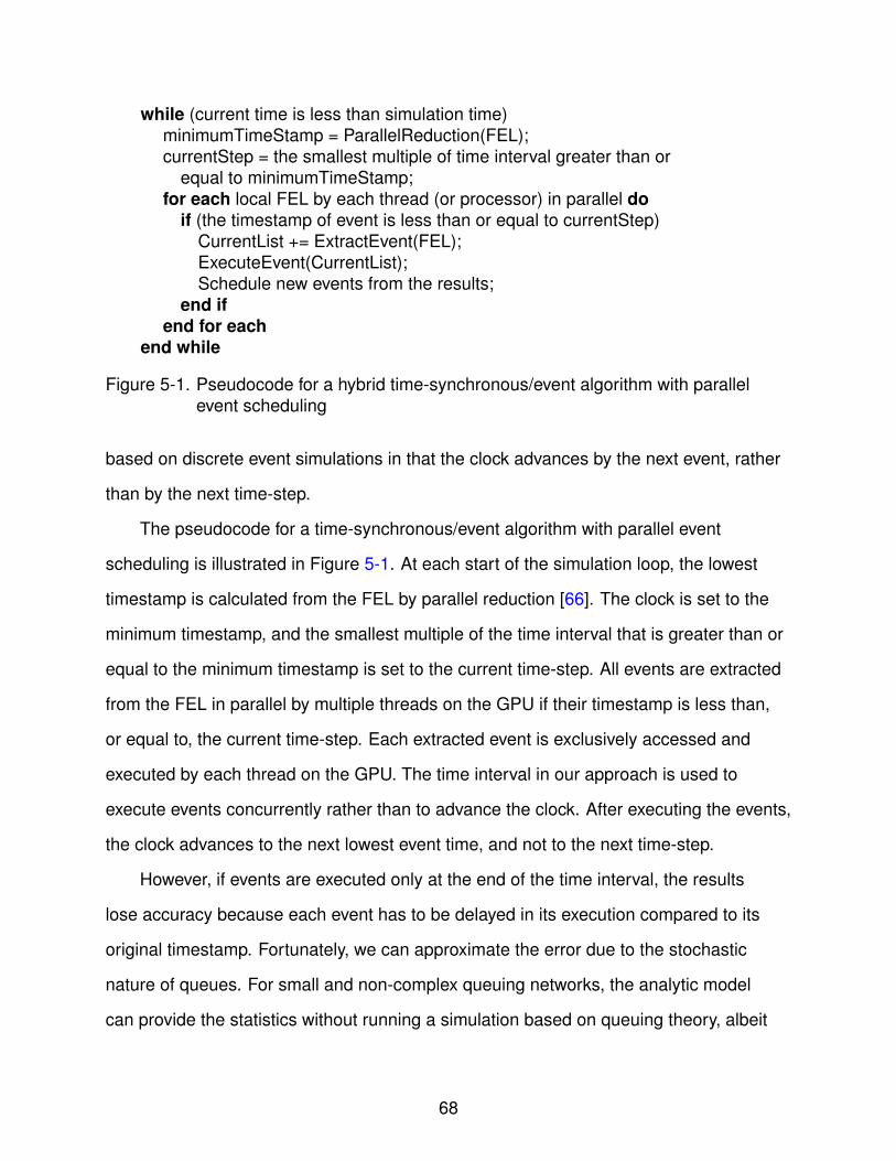
Transcript
PARALLEL DISCRETE EVENT SIMULATION OF QUEUING NETWORKS USINGGPU-BASED HARDWARE ACCELERATION
By
HYUNGWOOK PARK
A DISSERTATION PRESENTED TO THE GRADUATE SCHOOLOF THE UNIVERSITY OF FLORIDA IN PARTIAL FULFILLMENT
OF THE REQUIREMENTS FOR THE DEGREE OFDOCTOR OF PHILOSOPHY
UNIVERSITY OF FLORIDA
2009
c⃝ 2009 Hyungwook Park
2
To my family
3
ACKNOWLEDGMENTS
I would like to express my sincere gratitude to my advisor, Dr. Paul A. Fishwick for
his excellent inspiration and guidance throughout my Ph.D. studies at the University of
Florida. I would also like to thank my Ph.D. committee members, Dr. Jih-Kwon Peir, Dr.
Shigang Chen, Dr. Benjamin C. Lok, and Dr. Howard W. Beck for their precious time and
advice for my research. Also, I am grateful to the Korean Army. They gave me a chance
to study in the United States of America with financial support. I would like to thank my
parents, Hyunkoo Park and Oksoon Jung who encouraged me throughout my studies. I
would especially like to thank my wife, Jisuk Han, and my sons, Kyungeon and Sangeon
Park. They have been very supportive and patient throughout my studies. I would never
Abstract of dissertation Presented to the Graduate Schoolof the University of Florida in Partial Fulfillment of theRequirements for the Degree of Doctor of Philosophy
PARALLEL DISCRETE EVENT SIMULATION OF QUEUING NETWORKS USINGGPU-BASED HARDWARE ACCELERATION
By
Hyungwook Park
December 2009
Chair: Paul A. FishwickMajor: Computer Engineering
Queuing networks are used widely in computer simulation studies. Examples of
queuing networks can be found in areas such as the supply chains, manufacturing work
flow, and internet routing. If the networks are fairly small in size and complexity, it is
possible to create discrete event simulations of the networks without incurring significant
delays in analyzing the system. However, as the networks grow in size, such analysis
can be time consuming and thus require more expensive parallel processing computers
or clusters.
The trend in computing architectures has been toward multicore central processing
units (CPUs) and graphics processing units (GPUs). A GPU is the fairly inexpensive
hardware, and found in most recent computing platforms, but practical example of
single instruction, multiple data (SIMD) architectures. The majority of studies using
the GPU within the graphics and simulation communities have focused on the use
of the GPU for models that are traditionally simulated using regular time increments,
whether these increments are accomplished through the addition of a time delta
(i.e., numerical integration) or event scheduling using the delta (i.e., discrete event
approximations of continuous-time systems). These types of models have the property
of being decomposable over a variable or parameter space. In prior studies, discrete
event simulation, such as a queuing network simulation, has been characterized as
being an inefficient application for the GPU primarily due to the inherent synchronicity of
11
the GPU organization and an apparent mismatch between the classic event scheduling
cycle and the GPUs basic functionality. However, we have found that irregular time
advances of the sort common in discrete event models can be successfully mapped to
a GPU, thus making it possible to execute discrete event systems on an inexpensive
personal computer platform.
This dissertation introduces a set of tools that allows the analyst to simulate
queuing networks in parallel using a GPU. We then present an analysis of a GPU-based
algorithm, describing benefits and issues with the GPU approach. The algorithm
clusters events, achieving speedup at the expense of an approximation error which
grows as the cluster size increases. We were able to achieve 10-x speedup using our
approach with a small error in the output statistics of the general network topology. This
error can be mitigated, based on error analysis trends, obtaining reasonably accurate
output statistics.
12
CHAPTER 1INTRODUCTION
1.1 Motivations and Challenges
Queuing models [1–4] are constructed to analyze humanly engineered systems
where jobs, parts, or people flow through a network of nodes (i.e. resources). The
study of queuing models, their simulation, and their analysis is one of the primary
research topics studied within the discrete event simulation community [5]. There
are two approaches to estimating the performance and analysis of queuing systems:
analytical modeling and simulation [3, 5, 6]. An analytical model is the abstraction of
a system based on probability theory, representing the description of a formal system
consisting of equations used to estimate the performance of the system. However, it is
difficult to represent all situations in the real world using an analytical model because
that requires a restricted set of assumptions, such as an infinite number of queue
capacity and no bounds on the inter-arrival and service time, which do not often occur
in the real world. A simulation is often used to analyze the queuing system when a
theory for the system equations is unknown or the algorithm for the equations is too
complicated to be solved in closed-form. Computer simulation involves the formulation
of a mathematical model, often including a diagram. This model is then translated into
computer code, which is then executed and compared against a physical, or real-world,
system’s behavior under a variety of conditions.
Queuing model simulations can be expensive in terms of time and resources in
cases where the models are composed of multiple resource nodes and tokens that
flow through the system. Therefore, there is a need to find ways to speed up queuing
model simulations so that analyses can be obtained more quickly. Past approaches to
speeding up queuing model simulations have used asynchronous message-passing
with special emphasis on two approaches: the conservative and the optimistic
approaches [7]. Both approaches have been used to synchronize the asynchronous
13
logical processors (LPs), preserving causal relationships across LPs so that the results
obtained are exactly the same as those produced by sequential simulation. Most studies
of parallel simulation have been performed on multiple instruction, multiple data (MIMD)
machines, or related networks to execute the part of a simulation model or LP. The
parallel simulation approaches with partitioning the simulation model into several LPs
could easily be employed with a queuing model simulation, since the start of each
execution need not be explicitly synchronized with other LPs.
A graphics processing unit (GPU) is a processor that renders 3D graphics in real
time, and which contains several sub-processing units. Recently, the GPU has become
an increasingly attractive architecture for solving compute-intensive problems for general
purpose computation, which is called general-purpose computation on GPUs (GPGPU)
[8–11]. Availability as a commodity and increased computational power make the GPU
a substitute for expensive clusters of workstations in a parallel simulation, at a relatively
low cost. For much of the history of GPU development, there has been a need to map
the model into the graphics application programming interface (API), which limited the
availability of the GPU to those experts who had GPU- and graphics-specific knowledge.
This drawback has been resolved with the advent of the GeForce 8 series GPUs [12]
and compute unified device architecture (CUDA) [13, 14]. The control of the unified
stream processors on the GeForce 8 series GPUs is transparent to the programmer,
and CUDA provides an efficient environment to develop parallel codes in a high-level
language C without the need for graphics-specific knowledge.
In contrast to the previously ubiquitous MIMD approach to parallel computation
within the context of simulation research, the GPU is single instruction, multiple data
(SIMD)-based hardware that is oriented toward stream processing. SIMD hardware
is a relatively simple, inexpensive, and highly parallel architecture; however, there
are limits to developing an asynchronous model due to its synchronous operation.
Stream processing [15, 16] is the basic programming model of SIMD architecture. The
14
stream processing approach exploits data and task parallelism by mapping data flow to
processors, and provides efficient communication by accessing memory in a predictable
pattern using a producer-consumer locality as well. For these reasons, most simulation
models on the GPU are time-synchronous and compute-intensive models with stream
memory access.
However, queuing models are a typical asynchronous model, and their temporal
events are relatively fine-grained. Queuing models are usually simulated based on event
scheduling with manipulation of the future event list (FEL). Event scheduling tends to be
a sequential operation, which often overwhelms the execution times of events in queuing
model simulations. Another problem lies in the dynamic data structure for the event
scheduling method in discrete event simulations. Dynamic data structures cannot be
directly used on the GPU because dynamic memory allocation is not supported during
kernel execution. Moreover, the randomized memory access for individual data cannot
take advantage of massive parallelism on the GPU.
Nonetheless, the GPU can become useful hardware for facilitating fine-grained
discrete event simulations, especially for large-scale models, with the concurrent
utilization of a number of threads and fast data transfer between processors. The
execution time of each event can be very small, but a higher data parallelism with
clustering of the events can be achieved for a large-scale model.
The objective of this dissertation is to simulate asynchronous queuing networks
using GPU-based hardware acceleration. Two main issues related to this study are:
(1) how can we simulate asynchronous models on SIMD hardware? And (2) how can
we achieve a higher degree of parallelism? Investigations of these two main issues
reveal that further attention must be paid to the following related issues: (a) parallel
event scheduling, (b) data consistency without explicit support for mutual exclusion, (c)
event clustering, and (d) error estimation and correction. This dissertation presents an
approach to resolve these challenges.
15
1.2 Contributions to Knowledge
1.2.1 A GPU-Based Toolkit for Discrete Event Simulation Based on Parallel EventScheduling
We have developed GPU-based simulation libraries for CUDA so that the GPU can
easily be used for discrete event simulation, especially for a queuing network simulation.
A GPU is designed to process array-based data structures for the purpose of processing
pixel images in real time. The framework includes the functions for event scheduling and
queuing models that have been developed using arrays on the GPU.
In discrete event simulation, the event scheduling method occupies a large
portion of the overall simulation time. The FEL implementation, therefore, needs to
be parallelized in order to take full advantage of the GPU architecture. A concurrent
priority queue approach [17, 18] allows each processor to access the global FEL in
parallel on shared memory multiprocessors. The concurrent priority queue approach,
however, cannot be directly applied to SIMD-based hardware since the concurrent
insertion and deletion of the priority queue usually involves mutual exclusion, which is
not natively supported by GeForce 8800 GTX GPU [13].
Parallel event scheduling allows us to achieve significant speedup in queuing model
simulations on the GPU. A GPU has many threads executed in parallel, and each thread
can concurrently access the FEL. If the FEL is decomposed into many sub-FELs, and
each sub-FEL is exclusively accessed by one thread, the access to one element in the
FEL is guaranteed to be isolated from other threads. Exclusive access to each element
allows event insertion and deletion to be concurrently executed.
1.2.2 Mutual Exclusion Mechanism for GPU
We have reorganized the processing steps in a queuing model simulation by
employing alternate updates between the FEL and service facilities so that they can be
updated in SIMD fashion. The new procedure enables us to prevent multiple threads
16
from simultaneously accessing the same element, without having explicit support for
mutual exclusion on the GPU.
An alternate update is a lock-free method for mutual exclusion on the GPU, in order
to update two interactive arrays at the same time. Only one array can be exclusively
accessed by a thread index if the indexes of two arrays are not inter-related. If one array
needs to update the other array, the element in the other array is arbitrarily accessed by
the thread. Data consistency cannot be maintained if two or more threads concurrently
access the same element in the other array. The other array must be updated after
the thread index is switched to exclusively access itself. The updated array, however,
has to search all of the elements in the request array to find the request elements.
If the updated array knows which elements in the request array are likely to request
the update in advance, the number of searches will be limited. Each node in queuing
networks usually knows its incoming edges, which makes it possible to reduce the
number of searches during an alternate update, mitigating the overall execution time.
1.2.3 Event Clustering Algorithm on SIMD Hardware
SIMD-based simulation is useful when a lot of computation is required by a single
instruction with different data. However, its potential problems include the bottleneck in
the control processor and load imbalance among processors. The bottleneck problem
should not be significant when applying the CPU/GPU approach, since the CPU is
designed to process heavyweight threads, whereas the GPU is designed to process
lightweight threads and to execute arithmetic equations quickly [16].
The load imbalance problem can be resolved by employing a time-synchronous/event
algorithm in order to achieve a higher degree of parallelism. A single timestamp cannot
execute many events in parallel, since events in queuing models are irregularly spaced.
Thus, event times need to be modified so that they can be clustered and synchronized.
A time-synchronous/event algorithm is the SIMD-based hybrid approach to two common
types of discrete simulation: discrete event and time-stepped. The algorithm adopts the
17
advantages of both methods to utilize the GPU. The simulation clock advances when the
event occurs, but the events in the middle of the time interval are executed concurrently.
A time-synchronous/event algorithm naturally leads to approximation errors in the
summary statistics yielded from the simulation, because the events are not executed at
their precise timestamp.
We investigated three different types of queuing models to observe the effects of
our simulation method, including an implementation of a real-world application (mobile
ad hoc network model). The experimental results of our investigation show that our
algorithm has different impacts on the statistical results and performance of three types
of queuing models.
1.2.4 Error Analysis and Correction
The error in our simulation is a numerical error since we preserves timestamp
ordering and causal relationships of events, and the result is approximate in terms
of gathered summary statistics. The error may be acceptable for those modeled
applications where the analyst is more concerned with speed, and can accept relatively
small inaccuracies in summary statistics. In some cases, the error can be approximated
and potentially corrected to yield more accurate statistics. We present a method for
estimating the potential error incurred through event clustering by combining queuing
theory and simulation results. This method can be used to obtain a closer approximation
to the summary statistics through partially correcting the error.
1.3 Organization of the Dissertation
This dissertation is organized into 6 chapters. Chapter 2 reviews background
information, including the queuing model, sequential and parallel discrete event
simulation, GPU, and CUDA. Chapter 3 describes related work. We discuss other
studies for discrete event simulation on SIMD hardware, and a tradeoff between
accuracy and performance. Chapter 4 describes a GPU-based library and applications
framework for discrete event simulation. We introduce the routines that support parallel
18
event scheduling with mutual exclusion and queuing model simulations. Chapter
5 discusses a theoretical methodology and its performance analysis, including the
tradeoffs between numerical errors and performance gain, as well as the approaches
for error estimation and correction. Chapter 6 provides a summary of our findings and
introduces areas for future research.
19
CHAPTER 2BACKGROUND
2.1 Queuing Model
Queues are commonly found in most human-engineered systems where there exist
one or more shared resources. Any system where the customer requests a service for
a finite-capacity resource may be considered to be a queuing system [1]. The grocery
store, theme parks, and fast-food restaurants are well-known examples of queuing
systems. A queuing system can also be referred to as a system of flow. A new customer
enters the queuing system and joins the queue (i.e., line) of customers unless there is
no queue and another customer who completes his service may exit the system at the
same time. During the execution, a waiting line is formed in a system because the arrival
time of each customer is not predictable, and the service time often exceeds customer
inter-arrival times. A significant number of arrivals make each customer to wait in line
longer than usual. Queuing models are constructed by a scientist or engineer to analyze
the performance of a dynamic system where waiting can occur. In general, the goals of
a queuing model are to minimize the average number of waiting customers in a queue
and to predict the estimated number of facilities in a queuing system. The performance
results of queuing model simulation are produced at the end of a simulation in the form
of aggregate statistics.
A queuing model is described by its attributes [2, 6]: customer population, arrival
and service pattern, queue discipline, queue capacity, and the number of servers. A new
customer from the calling population enters into the queuing model and waits for service
in the queue. If the queue is empty and the server is idle, a new customer is immediately
sent to the server for service, otherwise the customer remains in the queue joining the
waiting line until the queue is empty and the server becomes idle. When a customer
enters into the server, the status of the server becomes busy, not allowing any more
20
Source
Arrival Departure
Customers wait for service
Queue
Server
Currently served customer
CallingPopulation
ArrivalPattern
QueueDiscipline
ServicePattern
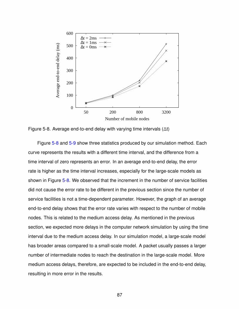
Figure 2-1. Components of a single server queuing model
arrivals to gain access to the server. After being served, a customer exits the system.
Figure 2-1 illustrates a single server queue with its attributes.
The calling population, which can be either finite or infinite, is defined as the pool
of customers who possibly can request the service in the near future. If the size of the
calling population is infinite, the arrival rate is not affected by others. But the arrival rate
varies according to the number of customers who have arrived if the size of the calling
population is finite and small. Arrival and service patterns are the two most important
factors determining behaviors of queuing models. A queuing model may be deterministic
or stochastic. For the stochastic case, new arrivals occur in a random pattern and their
service time is obtained by probability distribution. The arrival and service rates, based
on observation, are provided as the values of parameters for stochastic queuing models.
The arrival rate is defined as the mean number of customers per unit time, and the
service rate is defined by the capacity of the server in the queuing model. If the service
rate is less than the arrival rate, the size of the queue will grow infinitely. The arrival rate
must be less than the service rate in order to maintain a stable queuing system [1, 6].
21
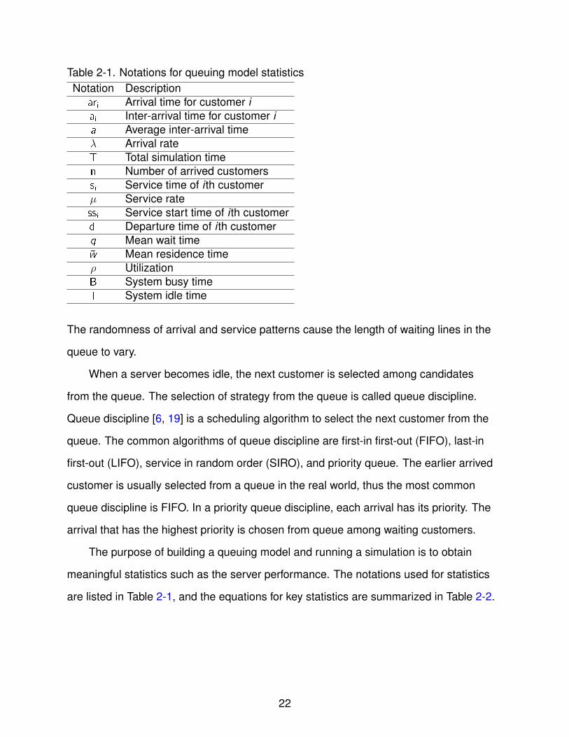
Table 2-1. Notations for queuing model statisticsNotation Description
ari Arrival time for customer iai Inter-arrival time for customer i�a Average inter-arrival time𝜆 Arrival rateT Total simulation timen Number of arrived customerssi Service time of i th customer𝜇 Service ratessi Service start time of i th customerdi Departure time of i th customer�q Mean wait time�w Mean residence time𝜌 UtilizationB System busy timeI System idle time
The randomness of arrival and service patterns cause the length of waiting lines in the
queue to vary.
When a server becomes idle, the next customer is selected among candidates
from the queue. The selection of strategy from the queue is called queue discipline.
Queue discipline [6, 19] is a scheduling algorithm to select the next customer from the
queue. The common algorithms of queue discipline are first-in first-out (FIFO), last-in
first-out (LIFO), service in random order (SIRO), and priority queue. The earlier arrived
customer is usually selected from a queue in the real world, thus the most common
queue discipline is FIFO. In a priority queue discipline, each arrival has its priority. The
arrival that has the highest priority is chosen from queue among waiting customers.
The purpose of building a queuing model and running a simulation is to obtain
meaningful statistics such as the server performance. The notations used for statistics
are listed in Table 2-1, and the equations for key statistics are summarized in Table 2-2.
22
Table 2-2. Equations for key queuing model statisticsName Equation Description
Inter-arrivalai = ari - ari−1
Interval between two consecutivetime arrivals
Mean�a =
∑ai
nAverage inter-arrival timeinter-arrival time
Arrival rate𝜆 =
n
TThe number of arrivals at unit time
𝜆 =1
�aLong run average
Mean�s =
∑si
n
Average time for each customer to beservice time served
Service rate 𝜇 =1
�sServer capability at unit time
Mean�q =
∑(ssi − ari)
n
Average time for each customer to spendwait time in a queue
Mean�w =
∑(di − ari)
n
Average time each customer stays in theresidence time system
SystemB =
∑si Total service time of serverbusy time
SystemI = T− B Total idle time of serveridle time
System𝜌 =
B
T
The proportion of the time in which theutilization server is busy
2.2 Discrete Event Simulation
2.2.1 Event Scheduling Method
Discrete event simulation changes the state variables at a discrete time when
the event occurs. An event scheduling method [20] is the basic paradigm for discrete
event simulation and is used along with a time-advanced algorithm. The simulation
clock indicates the current simulated time, the event time of last event occurrence. The
unprocessed, or future, events are stored in a data structure called the FEL. Events in
the FEL are usually sorted in non-decreasing timestamp order. When the simulation
starts, the head of the FEL is extracted from the FEL, updating the simulation clock. The
extracted event is then sent to an event routine, where it reproduces a new event after
23
(2) Update the clock
Event routine 1
Event routine 2
Event routine 3
Future event list (FEL)
NEXT_EVENTSimulation Clock
10 12
SCHEDULE
Token ID 5
Time 12
Event 2
Token ID 6
Time 15
Event 1
Token ID 3
Time 18
Event 3
(3) Execute the event
Token ID 5
Time 17
Event 3
(4) Insert new event into FEL
(1) Extract the head
from FEL
Figure 2-2. Cycle used for event scheduling
its execution. The new event is inserted to the FEL, sorting the FEL in non-decreasing
timestamp order. This step is iterated until the simulation ends.
Figure 2-2 illustrates the basic cycle for event scheduling [20]. Three future events
are stored into the FEL. When NEXT EVENT is called, token ID #5 with timestamp 12
is extracted from the head of the FEL. The simulation clock then advances from 10 to
12. The event is executed at event routine 2, which creates a new future event, event #3.
Token ID #5 with event #3 is scheduled and inserted into the FEL. Token ID #5 is placed
between token ID #6 and token ID #3 after comparing their timestamps. The event loop
iterates to call NEXT EVENT until the simulation ends.
The priority queue is the abstract data structure for an FEL. The priority queue
involves two operations for processing and maintaining the FEL: insert and delete-min.
The simplest way to implement the priority queue is to use an array or a linked list.
These data structures store events in a linear order by event time but are inefficient
24
for large-scale models, since the newly inserted event compares its event time with
all others in the sequence. An array and linked list takes O(N) time for insertion, and
O(1) time for deletion on average, where N is the number of elements in these data
structures. When an event is inserted, an array can be accessed faster than a linked list
on the disk, since the elements in arrays are stored contiguously. On the other hand, an
FEL using an array requires its own dynamic storage management [20].
The heap and splay tree [21] are data structures typically used for an FEL. They are
tree-based data structures and can execute operations faster than linear data structure,
such an array. Min heap implemented in a height-balanced binary search tree takes
O(log N) time for both insertion and deletion. A splay tree is a self-balancing binary tree,
but a certain elements can rearrange the tree, placing that element into the root. This
makes recently accessed elements able to be quickly referenced again. The splay tree
performs both operations in O(log N) amortized time. Heap and splay tree are therefore
suitable data structures for a priority queue for a large-scale model.
Calendar queues [22] are operated by a hash function, which performs both
operations in O(1), on average. Each bucket is a day that has a specific range and
each has a specific data structure for storing events in timestamp order. Enqueue and
dequeue functions are operated by hash functions according to event time. The number
of buckets and ranges in a day are adjusted to operate the hash function efficiently.
Calendar queues are efficient when events are equally distributed to each bucket, which
minimizes the adjustment of bucket size.
2.2.2 Parallel Discrete Event Simulation
In traditional parallel discrete event simulation (PDES) [7, 23, 24], the model
is decomposed into several LPs, and each LP is assigned to a processor used for
parallel simulation. Each LP runs its own independent part of the simulation with local
clock and state variables. When LPs need to communicate with each other, they send
timestamped messages to each other over a system bus or via a networking system.
25
Each local clock advances at different paces because the interval between consecutive
events on the LP is irregular. For this reason, the timestamp of incoming events from
other LPs can be earlier than the currently executed event. It is called a causality error
if the incoming events are supposed to change the state variable to which the current
event is referring. The violation of the causality error can produce different results.
As a result, a synchronization method needs to process events in a non-decreasing
timestamp order and to preserve causal relationships across processors. The
performance gains are not proportional to the increased number of processors due
to the synchronization overhead. Conservative and optimistic approaches are two main
categories in synchronization.
2.2.2.1 Conservative synchronization
In conservative synchronization methods, each processor executes events when it
can guarantee that other processors will not send events with a smaller timestamp than
that of the current event. Conservative methods can cause a deadlock situation between
LPs because every LP can block the event if it is considered to be unsafe to process.
Deadlock avoidance, and deadlock detection and recovery are two major challenges of
conservative synchronization methods.
Chandy and Misra [25] and Bryant [26] developed a deadlock avoidance algorithm.
The necessary and sufficient condition is that the messages are sent to other LPs over
the links in non-decreasing timestamp order, which guarantees that the processor will
not receive an event with a lower timestamp than the previous one. A null message is
sent to avoid the deadlock, indicating that the processor will not send a timestamped
message smaller than a null message. The timestamp of a null message is determined
by each incoming link, which provides the lower bound of the timestamp when the next
event occurs. The lower bound is determined by the knowledge of the simulation such
as lookahead, or the minimum timestamp increment for a message passing between
LPs. The variations of the null message method tried to reduce the number of null
26
messages based on demand since the amount of null message traffic can degrade
performance [27].
The deadlock detection and recovery proposed by Chandy and Misra [28] tried
to eliminate the use of null messages. The deadlock recovery approach allows the
processors to become deadlocked. When the deadlock is detected, the recovery
function is called. A controller, used to break the deadlock, identifies the event
containing the smallest timestamp among the processors, and sends the messages
to that LP indicating that the event is safe to process.
Barrier synchronization is one of the conservative synchronization approaches.
The lower bound on the timestamp (LBTS1 ) is calculated, based on the time of the next
event, and lookahead determines the time when all processors stop the execution to
safely process the event. The events are executed only if the timestamps of events are
less than LBTS. The distance between LPs is often used to determine LBTS since it
implies the minimum time to transmit the event from one LP to another, such as air traffic
simulation.
Conservative approaches are easy to implement but performance relies on
lookahead. Lookahead is the minimum time increment when the new event is scheduled,
thus lookahead (L) guarantees that no other events containing a smaller timestamp are
generated until the current clock plus L. Lookahead is used to predict the next incoming
events from other processors when the processor determines if the current event is safe.
If the lookahead is too small or zero, the currently executed event can cause all events
on the other LPs to wait. In this case, the events are nearly executed in sequential.
1 LBTS is defined as ”Lower bound on the timestamp of any message LP can receivein the future” in [7] p77.
27
2.2.2.2 Optimistic synchronization
In optimistic methods, each processor executes its own events regardless of those
received from other processors. However, each processor has to roll back the simulation
when it detects a causality error from event execution in order to recover the system.
Rollback in a parallel computing environment is a complicated process because some of
the messages sent to other LPs also need to be canceled.
Time-warp [29] is the most well-known scheme in optimistic synchronization. Time
warp has two major parts: the local and global control mechanisms. The local control
mechanism assumes that each local processor executes the events in timestamp order
using its own local virtual clock. When an LP sends a message to others, the identical
message, except for one field, is created. The original message sent from the LPs has a
positive sign, and its corresponding copy, called antimessage, has a negative. Each LP
maintains three queues. State queue contains the snapshots of the recent states at an
instant in time in the LP. The state is changed whenever the event occurs, and enqueued
at the state queue. Received messages from other LPs are stored at an input queue in
the timestamp order. The antimessage, produced by its own LP, is stored at the output
queue. When the timestamp of the arrival event is earlier than the local virtual time of
the LP, the LP encounters the causality error. The state is restored from state queue
prior to the timestamp of the current arrival message. Antimessages are dequeued
from the output queue and sent to other LPs, if their timestamps are between the arrival
event and the local virtual time. When the LP receives an antimessage, they annihilate
each other to cancel future events if the input queue contains the corresponding positive
message. The LP is rolled back by an antimessage if the corresponding positive
messages are already executed.
Global virtual time (GVT) gives an idea to solve some problems on local control
of the Time Warp mechanism, such as the memory management, the global control
of rollback and the safe commitment time. The GVT is defined by the minimum of
28
local virtual time among LPs and the timestamp of messages in transit, and serves
as a lower bound for the virtual times of the LPs. GVT allows the efficient memory
management because it does not need to maintain the previous states if those execution
times are earlier than the GVT. Duplicate antimessages are often produced while the
LP reevaluates the antimessages causing the problem of performance. The Lazy
cancelation waits to send the antimessage until the LP checks to see if the re-execution
produces the same messages, whereas Lazy reevaluation uses state vectors, instead of
messages, to solve this problem [7].
In the optimistic approach, the past states are saved for recovery, but it has one
of the most significant drawbacks regarding memory management. State saving [30]
makes copies of the past states during simulation. Copy state saving (CSS) copies the
entire states of simulation before each event occurs. CSS is the easiest method for
state saving, but two drawbacks are the huge memory consumption to save the entire
states and the performance overhead during rollback. Periodic state saving (PSS) sets
the checkpoint by interval skipping a few events. The performance is improved with
PSS, but all state values still have to be saved at the checkpoint. Incremental state
saving (ISS) is the method based on backtracking. Only the values and address of
modified variables are stored before the events execute. The old values are written to
the variables in reverse order when the states need to be restored. ISS reduces the
memory consumption and execution overheads, but the programmer has to add the
modules to handle each variable.
Reverse computation (RC) [31] was proposed to solve the limitation of the state
saving method for forward computation. RC does not save the values of state variables
during simulation. Computation is performed in reverse order to recover the values
of state variables until it reaches the checkpoint when the rollback is initiated. RC
uses the bit variable to check the changes, thus it can drastically reduce the memory
consumption during simulation for especially fine-grained models.
29
2.2.2.3 A comparison of two methods
Each synchronization approach has a drawback [32]. It takes considerable time to
run a simulation with zero lookahead in the conservative method. It is also too difficult to
roll back a simulation system to the previous state without error if we run the simulation
with a complicated model using the optimistic method. In general, the optimistic method
has an advantage over the conservative in that the execution is allowed where a
causality error is possible, but actually does not exist. In addition, the conservative
method often needs specific information for the application to determine when it is safe
to process the events, but it is not very relevant to an optimistic approach [23]. In some
cases, a very small lookahead cannot continue the simulation in parallel, but can in
sequential. Finding the lookahead and its size can be critical factors to determine the
performance gains in the conservative method [24]. However, optimistic mechanism
is much more complex to implement, and frequent rollback causes more computation
overhead for a compute-intensive system. If the model is too complex to apply the
optimistic method, the conservative method is a better choice. On the other hand, if a
very small lookahead is expected, the optimistic method has to be applied.
2.3 GPU and CUDA
2.3.1 GPU as a Coprocessor
A GPU is a dedicated graphics processor that renders 3D graphics in real time,
which requires tremendous computational power. The computation speed of the
GeForce 8800 GTX is approximately four times faster than that of an Intel Core2
Quad processor with 3.0 GHz, which is approximately twice as expensive as the
GeForce 8800 GTX [13]. The increment of the CPU clock speed has slowed since 2003
due to the physical limitations, so Intel and AMD turned their intention to multi-core
architectures [33]. On the other hand, the increment of GPU speed is still growing
because more transistors can be used for parallel data processing than data caching
and flow control on the GPU. Programmability is another reason that the GPU has
30
become attractive. The vertex and fragment processors can be customized with the
user’s own program.
The GPU has different features compared to the CPU [16]. The CPU is designed
to process general purpose programs. For this reason, CPU programming models
and their processes are generally serial, and the CPU enables the complex branch
controls. The GPU, however, is dedicated to processing the pixel image in real time,
thus it has much more parallelism than the CPU does. The CPU returns memory
reference quickly to process as many jobs as possible, maximizing its throughput and
minimizing the memory latency. As a result, a single thread on a CPU can produce
higher performance compared to that on a GPU. On the other hand, the GPU maximizes
the parallelism through threads. The performance of a single thread on a GPU is not as
good, compared to that on a CPU, but the executions of threads in a massively parallel
hide the memory latency to produce high throughput from parallel tasks. In addition,
more transistors are dedicated to GPU for data computation rather than data caching
and flow control. The GPU can take a great advantage over a CPU when the cache miss
occurs [34].
Despite many advantages, the harnessing power of the GPU has been considered
to be difficult because GPU-specific knowledge, such as graphics APIs and hardware,
needs to deal with the programmable GPU. The traditional GPUs have two types of
programmable processors: vertex and fragment [35]. Vertex processors transform
the streams of vertices which are defined by positions, colors, textures and lighting.
The transformed vertices are converted into fragments by the rasterizer. Fragment
processors compute the color of each pixel to render the image. Graphics shader
programming languages, such as Cg [36] and HLSL [37], allow the programmer to write
the code for the vertex and fragment processors in high-level programming language.
Those languages are easy to learn, compared to assembly language, but are still
graphic-specific assuming that the user has the basic knowledge of interactive graphic
31
programming. The program, therefore, needs to be written in a graphics fashion using
texture and pixel by mapping the computational variables to graphics primitives using
graphics API [38], such as DirectX or OpenGL even for general purpose computations.
Another problem was the constrained memory layout and access. The indirect
write or scatter operation was not possible because there is no write instruction in the
fragment processor [39]. As a result, the implementation of sparse data structure, such
as list and tree, where scattering is required, is problematic removing the flexibility
in programming. The CPU can handle the memory easily because it has the unified
memory model, but it is not trivial on the GPU because memory cannot be written
anywhere [35]. Finally, the advent of the GeForce 8800 GTX GPU and CUDA eliminates
the limitations and provides an easy solution to the programmer.
2.3.2 Stream Processing
Stream processing [15, 16] is the basis of the GPU programming model today. The
application of stream processing is divided into several parts for parallel processing.
Each part is referred to as a kernel, which is a programmed function to process
the stream and is independent of the incoming stream. The stream is a sequence
of elements composed of the same type and it requires the same instruction for
computation. Figure 2-3 shows the relationship between the stream and the kernel. The
stream processing model can process the input stream on each ALU at the same kernel
in parallel since each element of input stream is independent of each other. Also, stream
processing allows many streams to be processed concurrently at different kernels,
which hides the memory latency and communication delay. However, the stream
processing model is less flexible and not suitable for the general purpose program with
the randomized data access because the stream is directly passed to other kernels
connected in sequential after it is processed. Stream processing can consist of several
stages, each of which has several kernels. Data parallelism is exploited by processing
32
InputData
Kernel
KernelKernel
Kernel
KernelKernel
KernelKernelOutputData
Stream
Stream Stream
Stream
Stream
Stream
Stream
Figure 2-3. Stream and kernel
many streams in parallel at each stage and task parallelism is exploited by running
several stages concurrently.
Many cores can be utilized concurrently with a stream programming model. For
example, GeForce 8800 GTX has 16 multiprocessors, and each can have the maximum
768 threads. Theoretically, approximately ten thousand threads can be executed in
parallel yielding high performance parallelism.
2.3.3 GeForce 8800 GTX
The GeForce 8800 GTX [12, 13] GPU is the first GPU model unifying vertex,
geometry and fragment shaders into 128 individual stream processors. The previous
GPUs have the classic pipeline model with a number of stages to render the image
from the vertices. Many passes inside the GPU consume the bandwidth. Moreover,
some stages are not required to process general purpose computations, which degrade
the performance of the processing of the general purpose workloads on the GPU.
Figure 2-4 [40] illustrates the difference of pipeline stages between the traditional and
GeForce 8 series GPUs. In GeForce 8800 GTX GPU, the shaders have been unified
into the stream processors, which reduce the number of pipeline stages and change
the sequential processing into loop-oriented processing. Unified stream processors
help to improve load balancing. Any graphical data can be assigned to any available
33
Application
Display
Application
Display
Fragment
Rasterization
Vertex/Geometry
Command Command
RasterizationStream
Processors
ProgrammableProcessors
Figure 2-4. Traditional vs. GeForce 8 series GPU pipeline
stream processor, and its output stream can be used as an input stream of other stream
processors.
Figure 2-5 [41] shows the GeForce 8800 GTX architecture. The GPU consists of
16 stream multiprocessors (SMs). Each SM has 8 stream processors (SPs), which
makes a total of 128. Each SP contains a single arithmetic unit that supports IEEE 754
single-precision floating-point arithmetic and 32-bit integer operations, and can process
the instruction in SIMD fashion. Each SM can take up to 8 blocks or 768 threads, which
makes for a total of 12,288 threads, and 8192 registers on each SM can be dynamically
allocated into the threads running on it.
34
SP
SMInstruction
Unit
SharedMemory
SP
SMInstruction
Unit
SharedMemory
SP
SMInstruction
Unit
SharedMemory
SP
SMInstruction
Unit
SharedMemory
SP
SMInstruction
Unit
SharedMemory
SP
SMInstruction
Unit
SharedMemory
SP
SMInstruction
Unit
SharedMemory
SP
SMInstruction
Unit
SharedMemory
SP
SMInstruction
Unit
SharedMemory
SP
SMInstruction
Unit
SharedMemory
SP
SMInstruction
Unit
SharedMemory
SP
SMInstruction
Unit
SharedMemory
SP
SMInstruction
Unit
SharedMemory
SP
SMInstruction
Unit
SharedMemory
SP
SMInstruction
Unit
SharedMemory
SP
SMInstruction
Unit
SharedMemory
Global Memory
Thread Execution Manager
Figure 2-5. GeForce 8800 GTX architecture
2.3.4 CUDA
CUDA [13] is an API of C programming language for utilizing the NVIDIA class
of GPUs. CUDA, therefore, does not require a tough learning curve and provides
a simplified solution for those who are not familiar with the knowledge of graphics
hardware and API. The user can focus on the algorithm itself rather than on its
implementation with CUDA. When the program is written in CUDA, the CPU is a host
that runs the C program, and the GPU is a device that operates as a co-processor to the
CPU. The application is programmed into a C function, called kernel, and downloaded
to the GPU when compiled. The kernel uses memory on the GPU, memory allocation
and data transfer from the CPU to the GPU, therefore, need to be done before the kernel
invocation.
CUDA exploits data parallelism by utilizing a massive number of threads
simultaneously after partitioning larger problems into smaller elements. A thread is
the basic unit of execution that uses its unique identification to exclusively access parts
of elements in the data. The much smaller cost of creating and switching threads (as
compared to the higher costs associated with the CPU) makes the GPU more efficient
when running in parallel. The programmer organizes the threads in a two-level hierarchy.
35
A kernel invocation creates a grid (the unit of execution of a kernel). A grid consists of
the group of thread blocks that executes a single kernel with the same instruction and
different data. Each thread block consists of a batch of threads that can share data
with other threads through a low-latency shared memory. Moreover, their executions
are synchronized within a thread block to coordinate memory accesses by barrier
synchronization using the syncthreads() function. Threads in the same block need to
reside on the same SM for the efficient operation, which restricts the number of threads
in a single block.
In the GeForce 8800 GTX, each block can take up to 512 threads. The programmer
determines the degree of parallelism by assigning the number of threads and blocks for
executing a kernel. The execution configuration has to be specified when invoking the
kernel on the GPU, by defining the number of grids, blocks and bytes in shared memory
per block, in an expression of following form, where memory size is optional:
The corresponding function is defined by global void
KernelFunc(parameters) on the GPU, where global represents the computing
device or GPU. Data are copied from the host or CPU to global memory on the GPU
and are loaded to the shared memory. After performing the computation, the results are
copied back to the host via PCI-Express.
Each SM processes a grid by scheduling batches of thread blocks, one after
another, but block ordering is not guaranteed. The number of thread blocks in one batch
depends upon the degree to which the shared memory and registers are assigned,
per block and thread, respectively. The currently executed blocks are referred to as
active blocks, and each one is split into a group of threads called a warp. The number
of threads in a warp is called warp size and it is set to 32 on the GeForce 8 series. At
each clock cycle, the threads in a warp are physically executed in parallel. Each warp
is executed alternatively by time-slicing scheduling, which hides the memory access
36
Thread (0, 0)
Block (0, 0)
Grid 1
Thread (1, 0)
Thread (0, 1) Thread (1, 1)
Thread (0, 0)
Block (0, 0)
Grid 1
Thread (1, 0)
Thread (0, 1) Thread (1, 1)
Thread (0, 0)
Block (0, 0)
Grid 2
Thread (1, 0)
Thread (0, 1) Thread (1, 1)
SequentialExecution
SequentialExecution
SequentialExecution
KernelInvocation 2
KernelInvocation 1
Host
Device
Figure 2-6. Execution between the host and the device
latency. The number of thread blocks can increase if we can decrease the size of shared
memory per block and the number of registers per thread. However, it fails to launch the
kernel if the shared memory per thread block is insufficient.
The overall performance depends on how effectively the programmer assigns those
threads and blocks, keeping threads busy as many as possible. Each SM can usually be
composed of 3 thread blocks with 256 threads, or 6 blocks with 128 threads. The 16KB
shared memory is assigned to each thread block, which can limit the number of threads
in a thread block and the number of elements for which each thread is responsible.
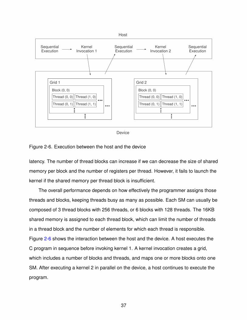
Figure 2-6 shows the interaction between the host and the device. A host executes the
C program in sequence before invoking kernel 1. A kernel invocation creates a grid,
which includes a number of blocks and threads, and maps one or more blocks onto one
SM. After executing a kernel 2 in parallel on the device, a host continues to execute the
program.
37
CHAPTER 3RELATED WORK
3.1 Discrete Event Simulation on SIMD Hardware
In the 1990s, efforts were made to parallelize discrete event simulations using a
SIMD approach. Given a balanced workload, SIMD had the potential to significantly
speed up simulations. The research performed in this area was focused on replication.
The processors were used to parallelize the choice of parameters by implementing a
standard clock algorithm [42, 43]. Ayani and Berkman [44] used SIMD for parallelizing
simultaneous event executions, but SIMD was determined to be a poor choice because
of the uneven distribution of timed events. There was a need to fill the gap between
asynchronous applications and synchronous machines so that the SIMD machine could
be utilized for asynchronous applications [45].
Recently, the computer graphics community has widely published on the use of the
GPU for physical and geometric problem solving, and for visualization. These types of
models have the property of being decomposable over a variable or parameter space,
such as cellular automata [46] for discrete spaces and partial differential equations
(PDEs) [47, 48] for continuous spaces. Queuing models, however, do not strictly adhere
to the decomposability property.
Perumalla [49] has performed a discrete event simulation on a GPU by running a
diffusion simulation. Perumalla’s algorithm selects the minimum event time from the
list of update times, and uses it as a time-step to synchronously update all elements
on a given space throughout the simulation period. This approach is useful if a single
event in the simulation model causes large amounts of computation, where the event
occurrences are not so frequent. Queuing models, in contrast, have many events, but
each event does not require significant computation. A number of events with different
timestamps in queuing model simulations could make the execution nearly sequential
with this algorithm.
38
Xu and Bagrodia [50] proposed a discrete event simulation framework for network
simulations. They used the GPU as a co-processor to distribute compute-intensive
workloads for high-fidelity network simulations. Other parallel computing architectures
are combined to perform the computation in parallel. A field programmable gate array
(FPGA) and a Cell processor are included for task-parallel computation, and a GPU
is used for data-parallel computation. A fluid-flow-based TCP and a high-fidelity
physical layer model are exploited to utilize the GPU. The former is modeled with
driven differential equations, and the latter uses the adaptive antenna algorithm which
recursively updates the weights of the beamformers using least squares estimation. The
event scheduling method on the CPU sends those compute-intensive events to the GPU
whenever events occur.
These two examples showed the methodology of running a discrete event
simulation on the GPU, but both methods cannot be applicable for the purpose of
improving the performance in queuing models simulations on the GPU. In the GPU
simulation, 2D or 3D spaces represent the simulation results, and these spaces are
implemented in arrays on the GPU. Their models are easily adapted to the GPU by
partitioning the result array and computing each of them in parallel since a single event
in their simulation models updates all elements in the result array at once. However, an
individual event in queuing models make the changes only on a single element (e.g.
service facility) in the result array, which makes it difficult to parallelize queuing model
simulations. Queuing model simulations need to have many concurrent events to benefit
from the GPU.
Lysenko and D’Souza [51] proposed a GPU-based framework for large scale agent
based model (ABM) simulations. In ABM simulation, sequential execution using discrete
event simulation techniques makes the performance too inefficient for large scale ABM.
Data-parallel algorithms for environment updates, and agent interaction, death, and birth
were, therefore, presented for GPU-based ABM simulation. This study used an iterative
39
randomized scheme so that agent replication could be executed in O(1) average time in
parallel on the GPU.
3.2 Tradeoff between Accuracy and Performance
Some studies of parallel simulation have focused on enhancing performance at the
expense of accuracy, while others have focused on accuracy with a view to improving
performance. Tolerant synchronization [52] uses the lock-step method to process the
simulation conservatively, but it allows the processor to execute the event optimistically
if the timestamp is less than the tolerance point in the synchronization. The recovery
procedure is not called, even if a causality error occurs, until the timestamp reaches the
tolerance point.
Synchronization with a fixed quantum is a lock-step synchronization [53] that
ensures that all events are properly synchronized before advancing to the next quantum.
However, a quantum that is too small causes a significant slowdown of overall execution
time. In an adaptive synchronization technique [54], the quantum size is adjusted based
on the number of events at the current lock-step. A dynamic lock-step value improves
the performance with a larger quantum value, thus reducing the synchronization
overhead when the number of events is small and where the error rate is low.
State-matching is the most dominant overhead in a time-parallel simulation [7],
as is synchronization in a space-parallel simulation. If the initial and final states are
not matched at the boundary of a time interval, re-computation of those time intervals
degrades simulation performance. Approximation simulations [55, 56] have been used to
improve the simulation performance, albeit with a loss of accuracy.
Fujimoto [32] proposed exploitation of temporal uncertainty, which introduces
approximate time. Approximate time is a time interval for the execution of the event,
rather than a precise timestamp, and assigned into each event based on its timestamp.
When approximate time is used, the time intervals of events on the different LPs can
be overlapped on the timeline at one common point. Whereas events on the different
40
LPs have to wait for a synchronization signal with a conservative method when a precise
timestamp is assigned, approximate-timed events can be executed concurrently if their
time intervals overlap with each other. The performance is improved due to increased
concurrency, but at the cost of accuracy in the simulation result. Our approach differs
from this method in that we do not assign a time interval to each event: instead, events
are clustered at a time interval when they are extracted from the FEL. In addition, an
approximate time is executed based on a MIMD scheme that partitions the simulation
model, whereas our approach is based on a SIMD scheme.
3.3 Concurrent Priority Queue
The priority queue is the abstract data structure that has widely been used as an
FEL for discrete event simulation. The global priority queue is commonly used and
accessed sequentially for the purpose of ensuring consistency in PDES on shared
memory multiprocessors. The concurrent access of the priority queue has been studied
because the sequential access limits the potential speedup in parallel simulation
[17, 18]. Most concurrent priority queue approaches have been based on mutual
exclusion, locking part of a heap or tree when inserting or deleting the events so that
other processors would not access the currently updated element [57, 58]. However, this
blocking-based algorithm limits potential performance improvements to a certain degree,
since it involves several drawbacks, such as deadlock and starvation, which cause
the system to be in idle or wait states. The lock-free approach [59] avoids blocking
by using atomic synchronization primitives and guarantees that at least one active
operation can be processed. PDES that use the distributed FEL or message queue
have improved their performance by optimizing the scheduling algorithm to minimize the
synchronization overhead and to hide communication latency [60, 61].
3.4 Parallel Simulation Problem Space
Parallel simulation problem space can be classified using time-space and classes
of parallel computers, as shown in Figure 3-1. Parallel simulation models fall into two
41
Continuous Discrete
Asynchronous Synchronous
MIMD
Parallel Simulation
Problem Space
SIMD GPUMIMD SIMD GPU MIMD SIMD GPU
Space Event
(1)
(10)(9)
(5) (6)(2) (3) (4) (7) (8)
Time/space
Behavior
Architecture
Examples
Partitioning
Method
Figure 3-1. Diagram of parallel simulation problem space
Table 3-1. Classification of parallel simulation examplesIndex Examples
(1) Ordinary differential equations [62](2) Reservoir simulation [63](3) Cloud dynamics [47], N-body simulation [48](4) Chandy and Misra [25], Time-warp [29](5) Ayani and Bourkman [44], Shu and Wu [45](6) Partial differential equations [64](7) Cellular automata [65](8) Retina simulation [46](9) Diffusion simulation [49], Xu and Bagrodia [50](10) Our queuing model simulation
major categories: continuous and discrete. Most physical simulations are continuous
simulations (i.e., ordinary and partial differential equations, cellular automata); however,
complex human-made systems (i.e., communication networks) tend to have a discrete
structure. Discrete models can be categorized into two, in regards to the behavior of
simulation models: asynchronous (discrete-event) and synchronous (time-stepped)
models. Asynchronous models can be classified according to how the partitioning is
done. The examples of each branch in Figure 3-1 are summarized in Table 3-1.
42
CHAPTER 4A GPU-BASED APPLICATION FRAMEWORK SUPPORTING FAST DISCRETE EVENT
SIMULATION
4.1 Parallel Event Scheduling
SIMD-based computation has a bottleneck problem in that some operations,
such as instruction fetch, have to be implemented sequentially, which causes many
processors to be halted. Event scheduling in SIMD-based simulation can be considered
as a step of instruction fetch that distributes the workload into each processor. The
sequential operations in a shared event list can be crucial to the overall performance
of simulation for a large-scale model. Most implementations of concurrent priority
queue have been run on MIMD machines. Their asynchronous operations reduce the
number of locks at the instant time of simulation. However, it is inefficient to implement
a concurrent priority queue with a lock-based approach on SIMD hardware, especially
a GPU because the point in time when multiple threads access the priority queue is
synchronized. It produces many locks that are involved in mutual exclusion, making their
operations almost sequential. Moreover, sparse and dynamic data structure, such as
heaps, cannot be directly developed on the GPU since the GPU is optimized to process
dense and static data structures such as linear arrays.
Both insert and delete-min operations re-sort the FEL in timestamp order. Other
threads cannot access the FEL during the sort, since all the elements in the FEL are
sorted if a linear array is used for the data structure of the FEL. The concept of parallel
event scheduling is that an FEL is divided into many sub-FELs, and only one of them
is handled by each thread on the GPU. An element index that is used to access the
element in the FEL is calculated by a thread ID combined with a block ID, which allows
each thread to access its elements in parallel without any interference from other
threads. In addition, keeping the global FEL unsorted guarantees that each thread
can access its elements, regardless of the operations of other threads. The number of
43
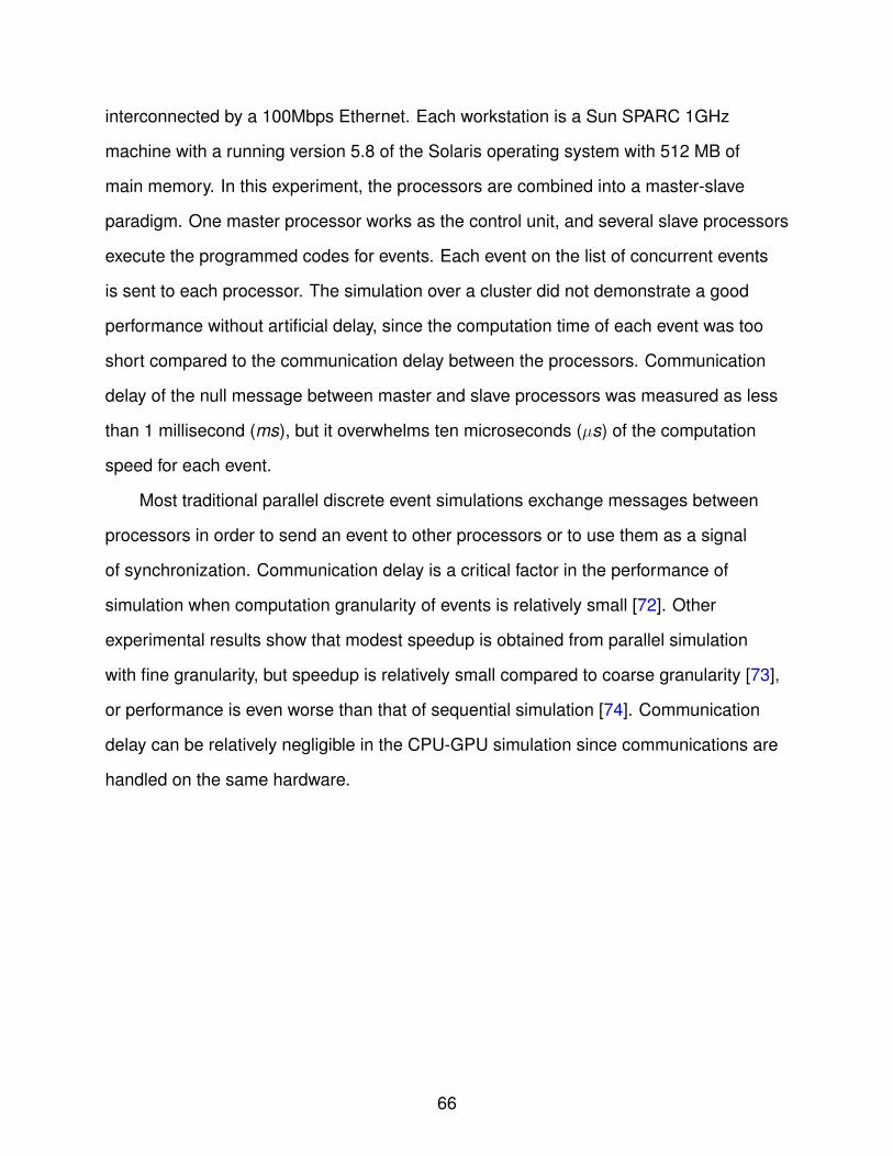
while (current time is less than simulation time)// executed by multiple threadsminimumTimestamp = ParallelReduction(FEL);for each local FEL by each thread in parallel do
In discrete event simulations, the time duration for each state is modeled as a
random variable [67]. Inter-arrival and service times in queuing models are the types
of variables that are modeled as specified statistical distributions. The Mersenne
twister [69] is used to produce the seeds for a pseudo-random number generator since
bitwise arithmetic and an arbitrary amount of memory writes are suitable for the CUDA
programming model [70]. Each thread block updates the seed array for the current
execution at every simulation step. Those seeds with statistical distributions, such
as uniform and exponential distributions, then produce the random numbers for the
variables.
4.4 Steps for Building a Queuing Model
This section describes the basic steps in developing the queuing model simulation.
Each step represents each kernel invoked from the CPU in sequence to develop the
mutual exclusion on the GPU. We have assumed that each service facility has only one
server for this example.
Step 1: Initialization The memory spaces are allocated for the FEL and service
facilities, and the state variables are defined by the programmer. The number of
elements for which each thread is responsible is determined by the problem size, as
well as by user selections, such as the number of threads in a thread block and the
number of blocks in a grid. Data structures for the FEL and service facility are copied to
the GPU, and initial events are generated for the simulation.
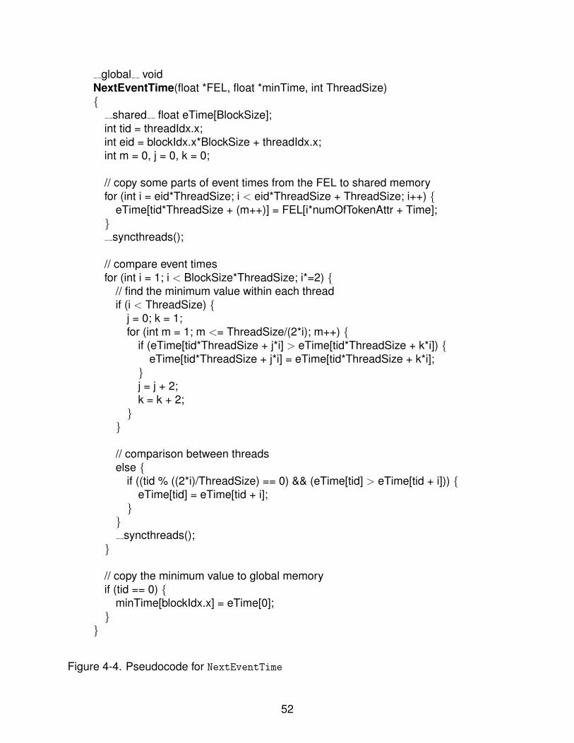
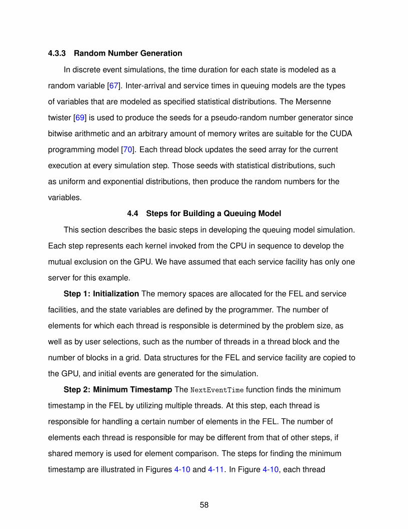
Step 2: Minimum Timestamp The NextEventTime function finds the minimum
timestamp in the FEL by utilizing multiple threads. At this step, each thread is
responsible for handling a certain number of elements in the FEL. The number of
elements each thread is responsible for may be different from that of other steps, if
shared memory is used for element comparison. The steps for finding the minimum
timestamp are illustrated in Figures 4-10 and 4-11. In Figure 4-10, each thread
58
#1, 5, A, 3 #2, 3, D, 1 #3, 6, D, 4 #4, 2, A, 6 #5, 2, D, 6 #6, 4, A, 5 #7, 6, D, 7 #8, 2, A, 8
Thread #1 Thread #2 Thread #3 Thread #4
ID, Time, Event (A: Arrival, D: Departure), Facility
Future Event List (FEL)
Figure 4-10. First step in parallel reduction
3 3 2 2 2 4 2 2
2 3 2 2 2 4 2 2
2 3 2 2 2 4 2 2
Event times in shared memory
Minimum event time
Figure 4-11. Steps in parallel reduction
compares two timestamps, and the smaller timestamp is stored at the left location.
The timestamps in the FEL are copied to the shared memory when they are compared
so that the FEL will not be re-sorted, as shown in Figure 4-11.
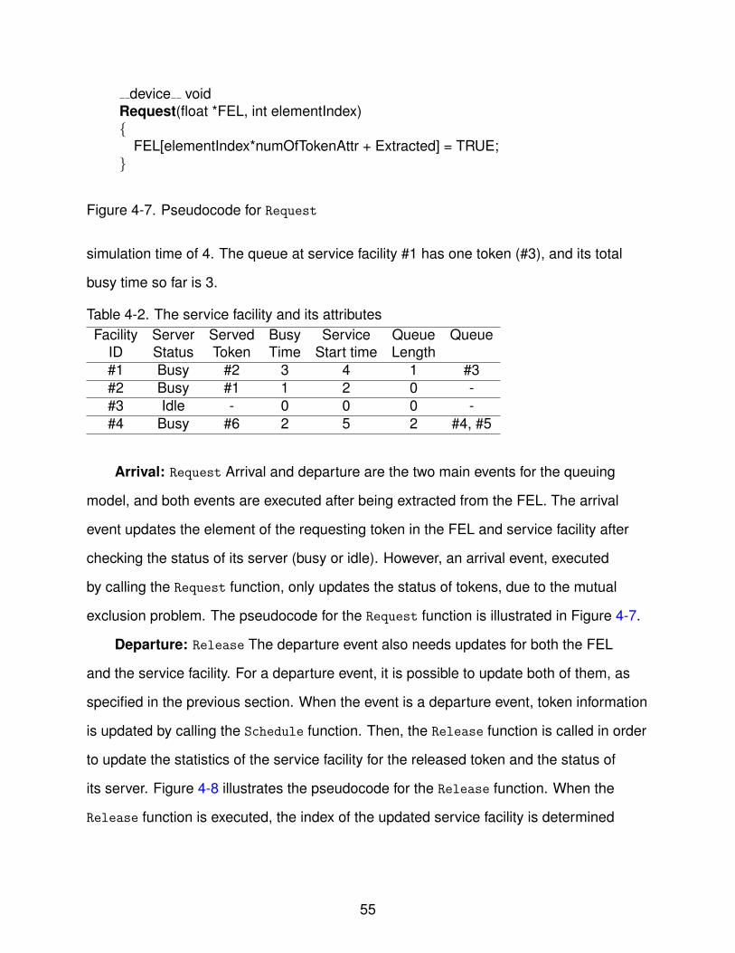
Step 3: Event Extraction and Departure Event The NextEvent function extracts
the events with the minimum timestamp. At this step, each thread is responsible for
handling a certain number of elements in the FEL, as illustrated in Figure 4-12. Two
main event routines are executed at this step. A Request function executes an arrival
event partially, just indicating that these events will be executed at the current iteration.
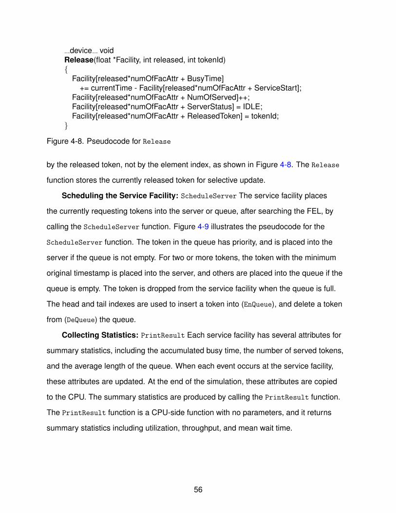
A Release function, on the other hand, executes a departure event entirely at this
step, since only one constant index is used to access the service facility for a Release
59
#1, 5, A, 3 #2, 3, D, 1 #3, 6, D, 4 #4, 2, A, 6 #5, 2, D, 6 #6, 4, A, 5 #7, 6, D, 7 #8, 2, A, 8
Thread #1 Thread #2 Thread #3 Thread #4
Future Event List (FEL)
#1, B, 2 #2, I, - #3, I, - #4, B, 3 #5, I, - #6, B, 5 #7, B, 7 #8, I, -
Service Facility
ID, Status (B: Busy, I: Idle), Token
ID, Time, Event (A: Arrival, D: Departure), Facility
#6, I, -
#5, 6, A, 1
Figure 4-12. Step 3: Event extraction and departure event
function. In Figure 4-12, tokens #4, #5, and #8 are extracted for future updates, and
service facility #6 releases token #5 at this step, updating both the FEL and service
facility at the same time. Token #5 is re-scheduled when the Release function is
executed.
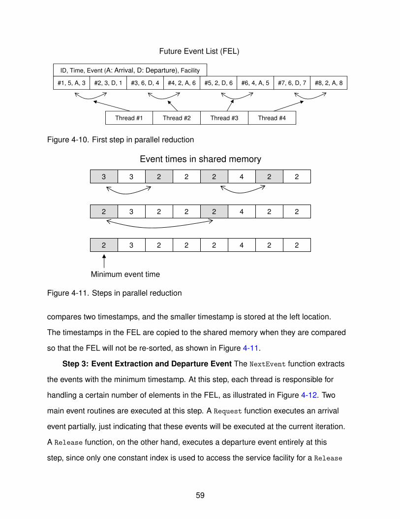
Step 4: Update of Service Facility The ScheduleServer function updates
the status of the server and the queue for each facility. At this step, each thread is
responsible for processing a certain number of elements in the service facility, as
illustrated in Figure 4-13. Each facility finds the newly arrived tokens by checking the
incoming edges and the FEL. If there is a newly arrived token at each service facility,
the service facilities with idle server (#2, #3, #5, #6, and #8) will place it into the server,
whereas the service facilities with busy server (#1, #4, and #7) will put it into the queue.
Token #8 is placed into the server of service facility #8. Token #4 can be located in the
server of service facility #6 because service facility #6 has already released token #5 at
the previous step.
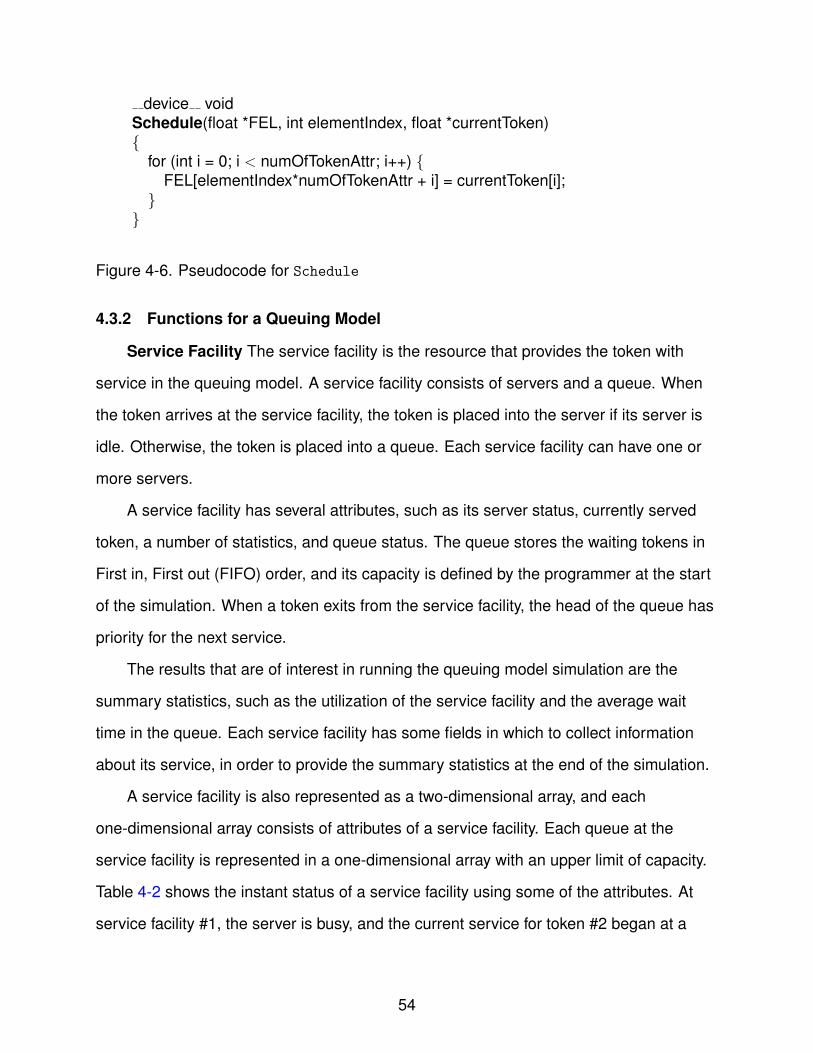
Step 5: New Event Scheduling The Schedule function updates the executed
tokens in the FEL. At this step, each thread is responsible for processing a certain
number of elements in the FEL, as illustrated in Figure 4-14. All tokens that have
60
#1, 5, A, 3 #2, 3, D, 1 #3, 6, D, 4 #4, 2, A, 6 #5, 6, A, 1 #6, 4, A, 5 #7, 6, D, 7 #8, 2, A, 8
Thread #1 Thread #2 Thread #3 Thread #4
Future Event List (FEL)
#1, B, 2 #2, I, - #3, I, - #4, B, 3 #5, I, - #6, I, - #7, B, 7 #8, I, -
Service Facility
ID, Status (B: Busy, I: Idle), Token
ID, Time, Event (A: Arrival, D: Departure), Facility
#6, B, 4 #8, B, 8
Figure 4-13. Step 4: Update of service facility
#1, 5, A, 3 #2, 3, D, 1 #3, 6, D, 4 #4, 2, A, 6 #5, 6, A, 1 #6, 4, A, 5 #7, 6, D, 7 #8, 2, A, 8
Thread #1 Thread #2 Thread #3 Thread #4
Future Event List (FEL)
#1, B, 2 #2, I, - #3, I, - #4, B, 3 #5, I, - #6, B, 4 #7, B, 7 #8, B, 8
Service Facility
ID, Status (B: Busy, I: Idle), Token
ID, Time, Event (A: Arrival, D: Departure), Facility
#4, 5, D, 6
#8, 7, D, 8
Figure 4-14. Step 5: New event scheduling
requested the service at the current time are re-scheduled by updating the attributes
of tokens in the FEL. Then, the control goes to Step 2, until the simulation ends. The
attributes of tokens #4 and #8 in Figure 4-14 are updated based on the results of the
previous step, as shown in Figure 4-13.
Step 6: Summary Statistics When the simulation ends, both arrays are copied to
the CPU, and the summary statistics are calculated and generated.
61
4.5 Experimental Results
The experimental results compare two parallel simulations with a sequential
simulation: the first is a parallel simulation with a sequential event scheduling method,
and the second is a parallel simulation with a parallel event scheduling method.
4.5.1 Simulation Environment
The experiment was conducted on an Intel Core 2 Extreme Quad 2.66GHz
processor with 3GB of main memory. The Nvidia GeForce 8800 GTX GPU [12] has
768MB of memory with a memory bandwidth of 86.4 GB/s. The CPU communicates
with the GPU via PCI-Express with a maximum of 4 GB/s in each direction. The C
version of SimPack [71] with a heap-based FEL was used in two sequential event
scheduling methods for comparison with parallel version. SimPack is a simulation
toolkit which supports the construction of various types of models and executing the
simulation, based on an extension of the general-purpose programming language. C,
C++, Java, JavaScript, and Python versions of SimPack have been developed. The
results represented in this dissertation are the average value of five runs.
4.5.2 Simulation Model
The toroidal queuing network model was used for the simulation. This application
is an example of a closed queuing network interconnected with a service facility.
Figure 4-15 shows an example of 3×3 toroidal queuing network. Each service facility
is connected to its four neighbors. When the token arrives at the service facility, the
service time is assigned to the token by a random number generator with an exponential
distribution. After being served by the service facility, the token moves to one of its
four neighbors, selected with uniform distribution. The mean service time of the facility
is set to 10 with exponential distribution, and the message population–the number of
initially assigned tokens per service facility–is set to 1. Each service time is rounded
to an integer so that many events are clustered into one event time. However, this will
introduce a numerical error into the simulation results because their execution times are
62
Figure 4-15. 3×3 toroidal queuing network
different to their original timestamps. The error may be acceptable in some applications,
but an error correction method may be required for more accurate results. In Chapter 5,
we analyze the error introduced by clustering events, and present the methods for error
estimation and correction.
4.5.3 Parallel Simulation with a Sequential Event Scheduling Method
In this experiment, the CPU and GPU are combined into a master-slave paradigm.
The CPU works as the control unit, and the GPU executes the programmed codes
for events. We used a parallel simulation method based on a SIMD scheme so that
events with the same timestamp value are executed concurrently. If there are two or
more events with the same timestamp, they are clustered into a list, and each event
on the list is executed by each thread. During the simulation, the GPU produces two
random numbers for each active token; the service time at the current service facility by
exponential distribution, and next service facility by uniform distribution. When the CPU
calls the kernel and passes the streams of active tokens, threads on the GPU generate
the results in parallel, and return them to the CPU. The CPU schedules the tokens using
these results.
Figure 4-16 shows the performance improvement in the GPU experiments. The
CPU-based simulation showed better performance in the 16×16 facilities because (1)
63
0.5
1
1.5
2
16×16 32×32 64×64 128×128 256×256 512×512
Spee
dup
Number of facilities
CPU-GPU simulationCPU-based simulation
Figure 4-16. Performance improvement by using a GPU as coprocessor
the sequential execution time in one time interval on the CPU was not long enough
compared to the data transfer time between the CPU and GPU (2) the number of events
in one time interval was not enough to maximize the number of threads on the GPU.
The GPU-based simulation outperforms the sequential simulation when (1) is satisfied,
and the performance increases when (2) is satisfied. However, the performance was
not good enough when we compare the results with other coarse-grained simulations.
In the SIMD execution, some parts of codes are processed in sequence, such as the
instruction fetch. The event scheduling method (e.g., the event insertion and extraction)
performed in sequence represents over 95% of the overall simulation time while the
event execution time (e.g., random number generation) is reduced by utilizing the GPU.
4.5.4 Parallel Simulation with a Parallel Event Scheduling Method
In the GPU experiment, the number of threads in the thread block is fixed at 128.
The number of elements that each thread processes and the number of thread blocks
are determined by the size of the simulation model. For example, there are 8 thread
blocks, and each thread only processes one element for both arrays in a 32×32 model.
64
0 1 2
5
10
14
16×16 32×32 64×64 128×128 256×256 512×512
Spee
dup
Number of facilities
GPU-based simulationCPU-GPU simulation
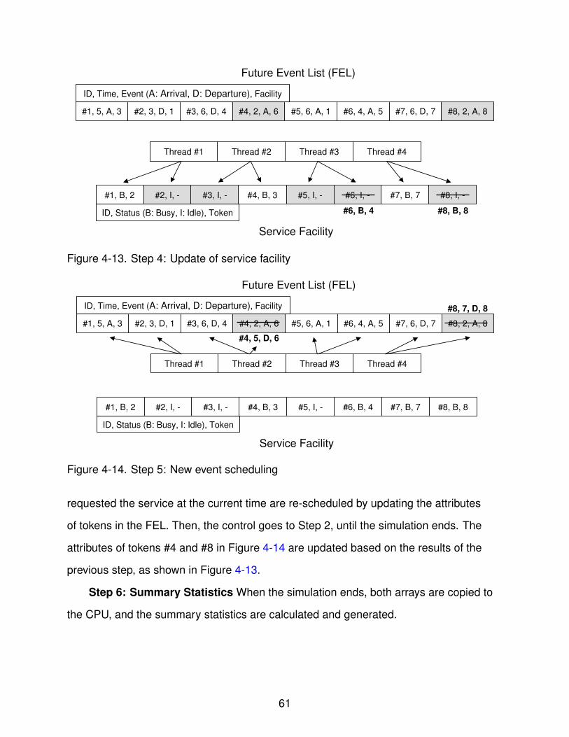
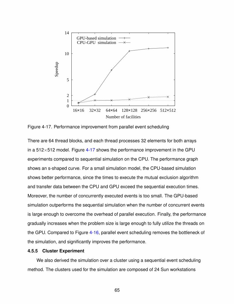
Figure 4-17. Performance improvement from parallel event scheduling
There are 64 thread blocks, and each thread processes 32 elements for both arrays
in a 512×512 model. Figure 4-17 shows the performance improvement in the GPU
experiments compared to sequential simulation on the CPU. The performance graph
shows an s-shaped curve. For a small simulation model, the CPU-based simulation
shows better performance, since the times to execute the mutual exclusion algorithm
and transfer data between the CPU and GPU exceed the sequential execution times.
Moreover, the number of concurrently executed events is too small. The GPU-based
simulation outperforms the sequential simulation when the number of concurrent events
is large enough to overcome the overhead of parallel execution. Finally, the performance
gradually increases when the problem size is large enough to fully utilize the threads on
the GPU. Compared to Figure 4-16, parallel event scheduling removes the bottleneck of
the simulation, and significantly improves the performance.
4.5.5 Cluster Experiment
We also derived the simulation over a cluster using a sequential event scheduling
method. The clusters used for the simulation are composed of 24 Sun workstations
65
interconnected by a 100Mbps Ethernet. Each workstation is a Sun SPARC 1GHz
machine with a running version 5.8 of the Solaris operating system with 512 MB of
main memory. In this experiment, the processors are combined into a master-slave
paradigm. One master processor works as the control unit, and several slave processors
execute the programmed codes for events. Each event on the list of concurrent events
is sent to each processor. The simulation over a cluster did not demonstrate a good
performance without artificial delay, since the computation time of each event was too
short compared to the communication delay between the processors. Communication
delay of the null message between master and slave processors was measured as less
than 1 millisecond (ms), but it overwhelms ten microseconds (𝜇s) of the computation
speed for each event.
Most traditional parallel discrete event simulations exchange messages between
processors in order to send an event to other processors or to use them as a signal
of synchronization. Communication delay is a critical factor in the performance of
simulation when computation granularity of events is relatively small [72]. Other
experimental results show that modest speedup is obtained from parallel simulation
with fine granularity, but speedup is relatively small compared to coarse granularity [73],
or performance is even worse than that of sequential simulation [74]. Communication
delay can be relatively negligible in the CPU-GPU simulation since communications are
handled on the same hardware.
66
CHAPTER 5AN ANALYSIS OF QUEUE NETWORK SIMULATION USING GPU-BASED
HARDWARE ACCELERATION
5.1 Parallel Discrete Event Simulation of Queuing Networks on the GPU
5.1.1 A Time-Synchronous/Event Algorithm
We used a parallel simulation method based on a SIMD scheme so that events
with the same timestamp value are executed concurrently. The simulation begins with
the extraction of the event with the lowest timestamp from an FEL. Event extraction
continues for as long as the next event has the same timestamp. Events with the same
timestamp are clustered into the current list of execution, and each event is executed
on each thread of the GPU. However, since it is unlikely that several events occur at
a single point of simulated time in a discrete event simulation, many threads will be
idle, resulting in wasted GPU resources and inefficient performance. We introduce a
time-synchronous/event algorithm using a time interval instead of a precise time, in
order to have more events occurring concurrently and reducing the load imbalance on
the threads of the GPU. Clustering events within a time interval makes it possible for
many more events to be executed at a single point of simulated time, which reduces the
number of idle threads and achieves more efficient parallel processing.
A time-synchronous/event algorithm that is used to cluster more events at a
single event time is a hybrid algorithm of discrete event simulations and time-stepped
simulations. The main difference between the two types of discrete simulation is the
method used to advance time. Our approach is similar to a time-stepped simulation in
the sense that we execute events at the end of the time interval to improve the degree of
parallelism. However, a time-stepped simulation can be inefficient if the state changes
in the simulation model occur irregularly, or if event density is low at the time interval.
Although there is no event at the next time-step, the clock must advance to the next
time-step, which reduces efficiency owing to idle processing time. Our approach is
67
while (current time is less than simulation time)minimumTimeStamp = ParallelReduction(FEL);currentStep = the smallest multiple of time interval greater than or
equal to minimumTimeStamp;for each local FEL by each thread (or processor) in parallel do
if (the timestamp of event is less than or equal to currentStep)CurrentList += ExtractEvent(FEL);ExecuteEvent(CurrentList);Schedule new events from the results;
end ifend for each
end while
Figure 5-1. Pseudocode for a hybrid time-synchronous/event algorithm with parallelevent scheduling
based on discrete event simulations in that the clock advances by the next event, rather
than by the next time-step.
The pseudocode for a time-synchronous/event algorithm with parallel event
scheduling is illustrated in Figure 5-1. At each start of the simulation loop, the lowest
timestamp is calculated from the FEL by parallel reduction [66]. The clock is set to the
minimum timestamp, and the smallest multiple of the time interval that is greater than or
equal to the minimum timestamp is set to the current time-step. All events are extracted
from the FEL in parallel by multiple threads on the GPU if their timestamp is less than,
or equal to, the current time-step. Each extracted event is exclusively accessed and
executed by each thread on the GPU. The time interval in our approach is used to
execute events concurrently rather than to advance the clock. After executing the events,
the clock advances to the next lowest event time, and not to the next time-step.
However, if events are executed only at the end of the time interval, the results
lose accuracy because each event has to be delayed in its execution compared to its
original timestamp. Fortunately, we can approximate the error due to the stochastic
nature of queues. For small and non-complex queuing networks, the analytic model
can provide the statistics without running a simulation based on queuing theory, albeit
68
with assumptions and approximations [1, 3]. We use queuing theory to estimate the
total error rate after we obtain the simulation results. The time interval can be another
parameter of the queuing model combined with two time-dependent parameters: arrival
and service rate. With the use of the time interval, the error rate caused by the time
interval is related to the arrival and service rates, and the amount of error depends
on the values of these parameters. The relationships between the time interval and
parameters are described in sections 5.3 and 5.4.
5.1.2 Timestamp Ordering
In parallel simulation, the purpose of synchronization is to process the events in
non-decreasing timestamps order to obtain the same results as those of a sequential
simulation. In a traditional parallel discrete event simulation, the event order can be
violated by the different speeds of event executions and communication delays between
processors, resulting in a causality error. Other simulation methods using the tradeoff
between accuracy and speedup allow the timestamp ordering to be violated within
certain limits, whereas our approach still keeps the timestamp ordering of events.
We do not need the explicit synchronization method since all the events are stored
in the global event list, and the time for each event execution is determined by the global
clock. The synchronous step of the simulation preserves the executions of events in a
non-decreasing timestamp order, blocking the event extractions from the FEL before
the current events finish scheduling the next events. The error caused by the time
interval, therefore, is different from the causality error because the timestamp ordering
is preserved, even though events are clustered at the end of the time interval. The
error in the result is the statistical error since each event does not occur at its precise
timestamp. However, a causality error can occur for the events with the same timestamp
when events are clustered by a time interval. Consider two or more tokens with different
timestamps requesting service at the same service facility. Their timestamps are
different, but they can be clustered into one time interval. In this case, an original
69
timestamp is used to determine the correct event order for simultaneous events. For
originally simultaneous events, the event order is randomly determined by each service
facility, as described in section 4.2.1.
5.2 Implementation and Analysis of Queuing Network Simulation
5.2.1 Closed and Open Queuing Networks
Queuing networks are classified into two types: closed and open [3]. In an open
queuing network, each token arrives at the system, based on the arrival rate, and
leaves the system after being served. On the other hand, the finite number of tokens
is assigned, and tokens are executed circulating the network in a closed queuing
network. Open queuing networks are more realistic queuing models than closed
queuing networks are, and communication network and traffic flow models [75] are
typical examples of these. However, closed queuing networks are widely used in the
modeling of a system where the number of tokens in the system has an impact on the
nature of the arrival process, due to the finite input populations [76]. CPU scheduling,
flexible manufacturing systems [77] and truck-shovel systems [78] are examples of
closed queuing networks.
The main difference between these two types of queuing networks is that the open
queuing network has new arrivals during the simulation. The number of tokens in the
open queuing network at any instant of time is always different due to the arrivals and
departures. The closed queuing network has a constant number of tokens during the
simulation since there are no new arrivals or departures. The error rate produced by the
use of a time interval will be different between the two types of queuing networks since
the number of tokens in the system affects the simulation results.
In the open queuing network, the arrival rate remains constant although the events
are only executed at the end of each time interval. A delayed execution time for each
event, compared to its precise timestamp, decreases the departure rate of the queuing
network, resulting in an increased number of tokens in the queuing network. As the
70
number of tokens in the queuing network increases, the wait time also increases since
the length of the queue at the service facility increases. In the closed queuing network,
we only need to consider the arrival and departure rates between the service facilities
since there is no entry from the outside. The delayed tokens arrive at the next service
facility as late as the difference between their original timestamps and actual execution
times. The length of the queue at the service facility remains unchanged by the time
interval since all tokens in the system are delayed at the same rate.
The implementation between closed and open queuing networks is also different.
It is possible to allocate a fixed size array for the FEL in the closed queuing network
because of the constant number of tokens during the simulation. A static memory
allocation with a fixed number of elements allows extraction of events from, and
re-scheduling into, the FEL to be performed on the GPU. The data need not be sent
back to the CPU in the middle of the simulation. In an open queuing network, the size
of the FEL is always different. For this reason the upper limit of memory for the FEL
needs to be estimated, which causes many threads on the GPU to be idle and memory
to be wasted. Moreover, the GeForce 8800 GTX GPU–the device of computer capability
1.0–does not support mutual exclusion and atomic functions [13]. The manual locking
method for concurrency control cannot be used when the interval between threads
that try to access the same element in memory is too short. The assignments of new
arrivals from outside of the queuing network to the shared resources of the FEL require
sequential execution so that multiple threads are prevented from concurrently accessing
and writing their new arrivals to the same empty location. In this case, newly arrived
tokens need to be generated on the CPU, resulting in data transfer between the CPU
and GPU. Both sequential execution and data transfer are a performance bottleneck,
and data transfer time can have a critical impact on performance in large-scale models.
The experimental results in Section 6 show these performance differences between a
closed and open queuing network.
71
On the other hand, if memory is separately allocated into the service facility
with external inputs from outside of the queuing network, then new arrivals can be
handled on the GPU. A location that is separate from other threads prevents them from
accessing the same location in the FEL. It is a feasible solution if there are few entries
from outside of the queuing network in the simulation model. Generally, this is not a
good approach for the large-scale model since memory allocation rapidly grows as the
number of service facilities increases.
5.2.2 Computer Network Model
The queuing model was originally developed to analyze and design a
telecommunication system [79], and has been frequently used to analyze the
performance of computer network systems. When a packet is sent from one node to
an adjacent node, there are four delays between the two nodes: processing, queuing,
transmission, and propagation delays [80]. Among these, the queuing delay is the most
studied delay because it is the only delay affected by the traffic load and congestion
pattern.
The time required for a packet to wait in the queue before being transmitted onto
the link is the queuing delay. In a computer network, the queuing delay includes the
medium access delay, which can increase the queuing delay. The medium access delay
is the time required for a packet to wait in the node until the medium is sensed as idle.
If another node connected to the same medium is transmitting packets, then a packet
in the first node cannot be transmitted, even if no packets are waiting in that queue.
Consequently, the shared medium is regarded as a common resource for the packets,
and the service facilities in the same medium are regarded as another queue for the
shared medium. Our simulation method causes the error rate to be higher due to the
two consecutive queues.
Figure 5-2 illustrates the possible delays caused by the time interval in the computer
network simulation when a packet is transmitted to the next node. In the general
72
Node Timeline
(1) Packet arrival,waits in queue
(5) Transmission timeby a time interval
(2) Originalexecution time
(4) End of backoff,original transmission time
(3) Execution timeby a time interval
d1 d2
Figure 5-2. Queuing delay in the computer network model
queuing model, d1 is the only delay caused by a time interval, but the packet cannot be
transmitted when the backoff time ends, and the medium is sensed as idle. The second
delay d2 is added onto the medium access delay, and it causes a greater error compared
to the general queuing model. The delays of other packets in the same medium also
make the d2 much longer.
The media access control (MAC) protocol [81] allows for several nodes to be
connected to the same medium and coordinates their accesses to the shared medium.
The implementation of the MAC protocol on the GPU can be different with respect to
the behaviors of the network. It is sufficient for each node only to sense the shared
medium in the sequential execution, but exclusive access to the shared medium by each
node needs to be guaranteed in the parallel execution. In a wired network, the network
topology is usually static, and the nodes connected to the same medium are also static
and not changed during the simulation. The MAC protocol in the simulation can be
developed to centrally control the nodes, which makes it possible for the MAC protocol to
be executed on the GPU using an alternate update.
The implementation of the MAC protocol in a wireless network with an access point
(AP) is not much different from in a wired network. The topology of mobile nodes is
dynamic, but that of APs is static. The nodes connected to the same AP are different
73
at any point in time, but the MAC protocol in the simulation can still be developed to
centrally control the nodes after searching all nodes currently connected to the AP.
However, a mobile ad hoc network (MANET) simulation [82] requires the distributed
implementation of the MAC protocol. The topology in MANETs is changed rapidly, and
the shared medium, which is determined by the transmission range of each mobile node
without any fixed AP, is completely different for each mobile node. The MAC protocol in
the simulation needs to be implemented with respect to each node. This requires the
sequential execution of the MAC protocol on the GPU, degrading the performance.
5.2.3 CUDA Implementation
A higher degree of parallelism can be achieved by concurrently utilizing many
stream multiprocessors on the GPU. A GPU implicitly supports data-level parallelism by
decomposing the computations into large pieces of small tasks and by guaranteeing the
threads exclusive access to each element. The FEL and service facility are two main
data structures in the queuing model, and these are represented as two-dimensional
arrays. One or more elements in both arrays are assigned to a single thread for parallel
execution. Each thread executes only the active events at the current time-step. A
GPU can process one kernel at a time, thus a task-level parallelism is required to
be implemented manually by combining two or more tasks in a single kernel, and by
dividing the thread blocks based on the number of tasks. In our MANET simulation,
the event extractions of data packet and location updates for each mobile node can be
programmed into a single kernel since the tasks are independent of each other, which
increases the utilization of threads.
Parallel processing is different from sequential processing in that many tasks are
concurrently executed, reducing the overall execution time. The problem needs to
be safely decomposed into sub-tasks so that each currently executed task does not
affect each other without changing the order of execution [83]. The FEL and service
facility have dependency in that two arrays need to be updated at the same time when
74
a request event is called. Arbitrary access to one array by multiple threads in parallel
allows multiple threads to concurrently access the same elements in the array. Their
executions need to be separated. Alternate updates between the FEL and service
facility have resolved this problem.
We need data transfer between the CPU and GPU to avoid simultaneous access
to shared resources since our GPU does not support mutual exclusion. The fast speed
of data transfer between the CPU and GPU via the PCI-Express bus has a significant
advantage over clusters with message passing between processors, which makes
the CPU with a GPU a more appropriate architecture for the simulation of fine-grained
events. However, the frequent data transfer between two devices can be a bottleneck in
the simulation. Data transfer time can be reduced by minimizing the size of data transfer,
which can be achieved by separating the array into two parts. The essential elements
which require sequential execution on the CPU are composed of a separate array that
has the index to the main array.
The size of the data structure needs to be static on the GPU. The number of service
facilities is constant during the simulation, whereas the number of elements in the FEL
of the open queuing network is always changed at any point in time. Concurrent access
to the elements in the FEL forces the generation of newly arrived tokens to be executed
on the CPU, which, however, makes it possible to dynamically adjust the size of the
FEL on the CPU at the start of each simulation loop. The array of the FEL can either be
doubled or cut in half, based on the number of tokens in the FEL.
We have made the most use of the data-parallel algorithms in NVIDIA CUDA SDK
[84] for our parallel queuing model simulation. A parallel reduction is used for finding
the minimum timestamp when extracting the events from the FEL, which allows us to
maintain the FEL without sorting it. The sequential execution of the MAC protocol on
the CPU does not need to search all the elements in the array if the array for the MAC
75
CallingPopulation
Server
Switch Server
Server Server Server
ServerServer
ServerServer
Figure 5-3. 3 linear queuing networks with 3 servers
protocol is sorted in a non-decreasing timestamp order. A bitonic sort on the GPU
allows us to search only the needed elements within the array.
5.3 Experimental Results
5.3.1 Simulation Model: Closed and Open Queuing Networks
When we ran a simulation using the time interval, we used two kinds of queuing
network models–closed and open queuing networks–to identify the differences of the
statistical results and performance between the two models. We first compared the
results of the closed queuing network with those of the open queuing network, and
analyzed the accuracy of the closed queuing network.
The first model is the queuing network of the toroidal topology used in section
4.5.2. The values of various parameters can be important factors affecting accuracy and
performance. We ran the simulation with varying values of two different parameters to
see the effects of these parameters on the statistical results. The open queuing network
consists of N linear queuing networks with k servers, as shown in Figure 5-3. A new
token arrives at the queuing network based on arrival rate 𝜆 from the calling population.
The newly arrived token is assigned to one of the linear queuing networks with uniform
distribution. After being served at the last server in the linear queuing network, the
token completes its job and exits the queuing network. The arrival and service times are
determined by exponential distribution.
76
5.3.1.1 Accuracy: closed vs. open queuing network
The values of the parameters and the number of service facilities for closed and
open queuing networks are configured to obtain similar results when the time interval is
set to zero. The results for various time intervals are compared with those of a zero time
interval to determine accuracy. The mean service time of the service facility is set to 10
with exponential distribution for both queuing networks. In the closed queuing network,
the message population–the number of initially assigned tokens per service facility–is
set to 1. In the open queuing network, the mean inter-arrival time from the calling
population is set to 20. We used the 32×32 topology as a basis for the experiments to
determine the accuracy.
Two summary statistics are presented in Figure 5-4 to show the difference by
using the time interval. Sojourn time is the average time a token to stay in one service
facility including the wait time in the queue. Utilization represents the performance of the
simulation model. In each subsequent plot, the time interval is on the horizontal axis. A
time interval of zero indicates no error in accuracy. As the interval increases, the error
also increases for the variable being measured on the vertical axis. Figure 5-4A shows
the average sojourn time of open and closed queuing networks for the time interval. It
takes much longer for a token to pass a service facility in the open queuing network,
since the number of tokens grows in the open queuing network, compared to the closed
queuing network as the time interval increases. Figure 5-4B shows the utilization for
the time interval. Utilization of the closed queuing network drops since arrivals for each
service facility are delayed due to the time interval, whereas utilization of the open
queuing network is almost constant since the arrival rate is constant regardless of
the time interval, and the increased number of tokens fills up possible idle time at the
service facility.
77
10
15
20
25
30
0 0.2 0.4 0.6 0.8 1
Sojo
urn
time
per
faci
lity
Time interval
Open queuing networkClosed queuing network
A Sojourn time
0.3
0.4
0.5
0.6
0.7
0 0.2 0.4 0.6 0.8 1
Util
izat
ion
Time interval
Open queuing networkClosed queuing network
B Utilization
Figure 5-4. Summary statistics of closed and open queuing network simulations
78
5.3.1.2 Accuracy: effects of parameter settings on accuracy
The time interval becomes one of the parameters in our simulation, and it causes
error by combining with other parameters. The time interval is a time-dependent
parameter, and it forces the execution time of each event to be delayed at the end of the
time interval. Time-dependent parameters, therefore, are said to be the primary factors
affecting the accuracy of a simulation. The closed queuing network was used for the
simulation to determine the effects of the parameter settings on accuracy.
Figure 5-5A shows the utilization with variations in the number of service facilities
for the time interval. The experimental results clearly show that the error rate is constant
regardless of the number of service facilities which is not a time-dependent parameter.
Figure 5-5B shows the utilization of the 32×32 toroidal queuing network, with variation in
the mean service time for the time interval. The variation of the mean service time–one
of time-dependent parameters–makes the error rate different. As the mean service time
increases, the ratio of the delay time by the time interval to the mean service time drops.
The error, therefore, decreases as the mean service time increases for the same time
interval. Interestingly, the error rate in Figure 5-5B is determined by the ratio of the mean
service time to the time interval. The utilizations are almost same in the following three
cases:
∙ Mean service time: 5. Time interval: 0.2
∙ Mean service time: 10. Time interval: 0.4
∙ Mean service time: 20. Time interval: 0.8
Figure 5-5B implies that the error rate can be estimated based on the fact that
the error rate is regular for the same ratio of a time-dependent parameter to the time
interval.
5.3.1.3 Performance
The performance was calculated by comparing the runtime of a parallel simulation
with that of a sequential simulation. We can expect better performance as the time
79
0.3
0.4
0.5
0.6
0.7
0 0.2 0.4 0.6 0.8 1
Util
izat
ion
Time interval
128×128 nodes 64× 64 nodes 32× 32 nodes
A Utilization with varying the number of facilities
0.3
0.4
0.5
0.6
0.7
0 0.2 0.4 0.6 0.8 1
Util
izat
ion
Time interval
mean service time = 20mean service time = 10mean service time = 5
B Utilization with varying the mean service time
Figure 5-5. Summary statistics with varying parameter settings
80
interval increases since many events are clustered at one time interval; however, a large
time interval also introduces more errors in the results.
Figure 5-6A shows the improvement in the performance of closed queuing network
simulations for the number of service facilities and the time interval, with the same
values of parameters that were used in Figure 5-4. This graph indicates that the
performance improvement depends on the number of events in one time interval.
As expected, a larger time interval leads to better performance. For a very small-scale
model, especially 16×16 topology, the number of threads that run concurrently is too
small. As a result, the overheads of parallel execution, such as mutual exclusion and
CPU-GPU interactions, exceed the sequential execution times. The parallel simulation
outperforms the sequential simulation when the number of clustered events in one
time interval is large enough to overcome the overheads of parallel execution. Not
all participant threads can be fully utilized in a discrete event simulation, since only
extracted events are executed at once. A large time interval keeps more participant
threads busy, resulting in an increasing number of events in one time interval. The
performance, therefore, increases in proportion to the increment of the time interval.
Finally, the performance improvement gradually increases when the number of events in
one time interval is large enough to maximize the number of threads executed in parallel
on the GPU. In a 512×512 topology, the number of events in the FEL is too large to
be loaded into the shared memory on the GPU at a time during the parallel reduction,
which limits the performance improvements compared to the 256×256 topology.
Figure 5-6B shows the speedup of open queuing network simulations for the
number of service facilities and the time interval, with the same values of parameters
that were used in Figure 5-4. The shapes of the curves are very similar to those of
closed queuing network simulations, except for the magnitude of speedup. The
overheads of sequential execution for newly arrived tokens on the CPU and of data
transfer between the CPU and GPU result in a degradation of performance in the
81
0 1 2
5
10
14
16×16 32×32 64×64 128×128 256×256 512×512
Spee
dup
Number of facilities
∆t = 1.0∆t = 0.5∆t = 0.2∆t = 0.1
A Closed queuing network
0 1 2
5
10
14
16×16 32×32 64×64 128×128 256×256 512×512
Spee
dup
Number of facilities
∆t = 1.0∆t = 0.5∆t = 0.2∆t = 0.1
B Open queuing network
Figure 5-6. Performance improvement with varying time intervals (�t)
simulation of an open queuing network. The experimental results indicate that the
relationship between the error rate and performance improvement is model-dependent
and implementation-dependent; hence it is not easy to formalize.
82
Parallel overheads in our experimental results are summarized below.
∙ Thread synchronization between event times
∙ Reorganization of simulation steps for mutual exclusion
∙ Data transfer between the CPU and the GPU
∙ Sequential execution on the CPU to avoid simultaneous access to sharedresources
∙ Load imbalance between threads at each iteration
5.3.2 Computer Network Model: a Mobile Ad Hoc Network
5.3.2.1 Simulation model
A MANET is a self-configuring network composed of mobile nodes without any
centralized infrastructure. Each mobile node directly sends the packet to other mobile
nodes in a MANET. Each mobile node relays the packet to its neighbor node when the
source and destination nodes are not in transmission range of each other. Figure 5-71
illustrates the difference between wireless and mobile ad hoc networks. In a wireless
network, each mobile node is connected to an AP and communicates with other mobile
nodes via the AP. Figure 5-7A shows that node #1 can communicate with node #3 via
two APs in a wireless network. On the other hand, node #1 can communicate with node
#3 via nodes #2 and #4 in a MANET, as shown in Figure 5-7B.
When a mobile node sends the packet, it is relayed by intermediate nodes to reach
the destination node, using a routing algorithm. The development of an effective routing
algorithm can reduce the end-to-end delay as well as the number of hop counts, thus
minimizing congestion of the network. For this reason, A MANET is often developed to
evaluate the routing algorithm. A MANET simulation requires many more computations
than a traditional wired network simulation because of its mobile nature. The locations
1 Each circle represents the transmission range of each mobile node or AP.
83
Node #1 Node #3
AP AP
Node #2N d #4
Node #2Node #4
A Wireless network
Node #1N d #3
Node #1Node #3
Node #2
Node #4
B Mobile ad hoc network
Figure 5-7. Comparison between wireless and mobile ad hoc networks
84
of mobile nodes are always changing, which makes the topology different at any point
in time. A routing table in each mobile node, therefore, must be frequently updated.
A routing algorithm requires a beacon signal to be transmitted between mobile nodes
to update the routing table. A MANET simulation can benefit from a GPU because it
requires heavy computations with frequent location updates of each mobile node and
routing table. We have developed the MANET simulation model with a routing algorithm,
mobility behavior, and MAC protocol to run the packet-level simulation.
Routing Algorithm: Greedy Perimeter Stateless Routing (GPSR) [85] is used
to implement the routing algorithm in a MANET. Each mobile node maintains only its
neighbor table. When the mobile node receives a greedy mode packet for forwarding,
it transmits the packet to the neighbor whose location is geographically closest to the
destination. If the current node is the closest node to the packet’s destination, the packet
is turned to a perimeter mode. The packet in the perimeter mode traverses the edges
in the planar graph by applying the right-hand rule. The packet returns to the greedy
mode when it reaches the node that is geographically closer to the destination than
the mobile node that previously set the packet to the perimeter mode. Each mobile
node broadcasts the beacon signal periodically to acknowledge its location to the
neighbors. Those mobile nodes that receive the beacon signal update their neighbor
table. Each mobile node transmits the beacon signal every 0.5 to 1.5 seconds. The
detailed algorithm is specified in Karp and Kung [85].
Mobility: The mobility of a mobile node is modeled by the random waypoint mobility
model [86]. A mobile node chooses a random destination with a random speed which is
uniformly distributed between 0 and 20 m/s. When the node arrives at its destination, it
stays for a certain period of time before selecting a new destination. The pause time is
uniformly distributed between 0 and 20 seconds.
MAC Protocol: The mobile node can transmit the packet if none of mobile nodes
within the transmission range currently transmits the packet. Each mobile node senses
85
Table 5-1. Simulation scenarios of MANETNumber of mobile nodes 50 200 800 3200
Region (m×m) 1500×600 3000×1200 6000×2400 12000×4800Node density 1 node / 9000 m2
inter-arrival time of the next service facility increases by an average of d. The utilization
of the M/M/1 queue is defined by 𝜆𝜇, where 𝜆 and 𝜇 refer to the arrival and service rates,
respectively [1]. The equation can also be defined by s
a, where s and a refer to the
service time and inter-arrival time, respectively. Consider the linear queuing network with
two queues, and yield statistics at an instant in time. The equation of utilization (𝜌2) for
the second queue is defined by equation (5–1) since the instant of inter-arrival time at
the second queue is the sum of the service time at the first queue and the delay time by
the time interval (𝛿).
𝜌2 =s
a + d(5–1)
91
Let an error rate denote the rate of decrease in utilization by the time interval. The error
rate e can be defined by equation (5–2).
e =𝜌2𝜌1
=a
a + d, where 𝜌1 =
s
aand 𝜌2 =
s
a + d(5–2)
To calculate an average d, we have to consider the probability P0 that the service facility
does not contain a token. In the open queuing network, the increased number of tokens
due to the time interval causes the probability P0 to drop, thus d increases exponentially.
In the closed queuing network, the probability P0 is not affected by the time interval
since all tokens are delayed, reducing the arrival rate to each service facility. All tokens
have to wait until the end of the time interval, thus the d of a long-run time-average is
𝛿/2. The decline in utilization is affected by half the time interval. The inter-arrival time of
a long-run time-average �a in equation (5–2) approaches �s, the service time of a long-run
time-average. When we substitute d = 𝛿/2 into the equation (5–2), the error rate e is
defined by
e =�s
�s + 𝛿/2(5–3)
The utilization with the time interval, 𝜌(𝛿) is defined by equation (5–4), where 𝛿0 refers to
a zero time interval.
𝜌(𝛿) =�s
�s + 𝛿/2× 𝜌(𝛿0) =
𝜌(𝛿0)
1 + 𝜇𝛿/2(5–4)
Consequently, we can derive the equation to correct the error in utilization. The original
value of the utilization in the toroidal queuing network can be approximated by
𝜌(𝛿0) = (1 + 𝜇𝛿/2)× 𝜌(𝛿) (5–5)
Figure 5-12 shows the comparison of the error rate between the experimental
and estimated results for two cases of the mean service time. As the ratio of the
mean service time to time interval increases, the difference between the two results
decreases. Figure 5-13 shows the results calculated by equation (5–5) of the error
correction method with the experimental results in Figure 5-12. The graph indicates
92
0.2
0.3
0.4
0.5
0.6
0 0.2 0.4 0.6 0.8 1
Util
izat
ion
Time interval
mean service time = 20, experiment estimation
mean service time = 5, experiment estimation
Figure 5-12. Comparison between experimental and estimation results
0.2
0.3
0.4
0.5
0.6
0 0.2 0.4 0.6 0.8 1
Util
izat
ion
Time interval
mean service time = 20mean service time = 5
Figure 5-13. Result of error correction
that we can significantly reduce the error by the error correction method. For the mean
service time of 20, the error rate is only 0.6% at the time interval of 1.
93
The equation of the utilization for error correction is not derived from the analysis
of individual nodes. Our intention is to approximate the total error rate when adding
one more parameter–time interval–so that the error is corrected to yield more accurate
results. The equation for the total error rate is derived from the equations of queuing
theory. The equation combined with the results from the simulation produces more
accurate results without building a complicated analytical model from each node.
94
CHAPTER 6CONCLUSION
6.1 Summary
We have built a CUDA-based library to support parallel event scheduling and
queuing model simulation on a GPU, and introduced a time-synchronous/event
approach to achieve a higher degree of parallelism. There has been little research
in the use of a SIMD platform for parallelizing the simulation of queuing models. The
concerns in the literature regarding event distribution and the seemingly inappropriate
application of GPUs for discrete event simulation are addressed (1) by allowing events
to occur at approximate boundaries at the expense of accuracy, and (2) by using a
detection and compensation approach to minimize error. The tradeoff in our work is that
while we get significant speedup, the results are approximate and result in a numerical
error. However, in simulations where there is flexibility in the output results, the error
may be acceptable.
The event scheduling method occupies a significant portion of computational
time in discrete event simulations. A concurrent priority queue approach allowed each
processor to simultaneously access the global FEL on shared memory multiprocessors.
However, an array-based data structure and synchronous executions among threads
without explicit support for mutual exclusion prevented the concurrent priority queue
approach from being directly applied to the GPU. In our parallel event scheduling
method, the FEL is divided into many sub-FELs, which allows threads to process these
smaller units in parallel by utilizing a number of threads on a GPU without invoking
sophisticated mutual exclusion methods. Each element in the array holds its position
while the FEL remains unsorted, which guarantees that each element is only accessed
by one thread. In addition, alternate updates between the FEL and service facilities in a
queuing model simulation allow both shared resources to be updated bi-directionally on
the GPU, thereby avoiding simultaneous access to the shared resources.
95
We have simulated and analyzed three types of queuing models to see what
different impacts they have on the statistical results and performance using our
simulation method. The experimental results show that we can achieve up to 10 times
the speedup using our algorithm, although the increased speed comes at the expense of
accuracy in the results. The relationship between accuracy and performance, however,
is model dependent, and not easy to define on a more general basis. In addition, the
statistical results in MANET simulations show that our method only causes an error in
the time-dependent statistics. Although the improvement of performance introduced
an error into the simulation results, the experimental results showed that the error
in queuing network simulations is regular enough to apply in order to estimate more
accurate results. The time interval can be one of the parameters used to produce the
results, and so the error can be approximated with the values of the parameters and
topologies of the queuing network. The error produced by the time interval can be
mitigated using results from queuing theory.
6.2 Future Research
The current GPUs and CUDA provide programmers with an efficient framework of
parallel processing for general purpose computations. A GPU can be more powerful
and cost-effective than other parallel computers if it is efficiently programmed. However,
parallel programming on GPUs may still be inconvenient for programmers, since all
general algorithms and programming techniques cannot be directly converted and used.
We can further improve the performance of queuing network simulations by
removing more sequential executions from the GPU. The magnitude of the performance
depends on how much we can reduce sequential executions in the simulation. In this
study, we were able to completely remove sequential executions in the simulation of
the closed queuing network. However, the synchronous executions of multiple threads
require at least some code to be sequential. Thus, removing sequential execution in the
programming codes not only improves performance, but also reduces the error in the
96
statistical results, since we can achieve considerable speedup with a small time interval.
We will be able to convert some sequential code to the parallel code related to data
inconsistency, using atomic functions for devices of compute capability 1.1 and above.
However, we still need parallel algorithms to process the remaining sequential code (e.g.
MAC protocol in MANET simulations) in parallel.
Error analysis for real applications is more complex than it is for the example of the
toroidal queuing network, since the service rates of each service facility are different,
and also because there are many parameters to be considered. For these reasons, it
is difficult to capture the characteristics of the complex simulation models. Our future
research will include more studies for error estimation and correction methods in regards
to various applications.
97
REFERENCES
[1] L. Kleinrock, Queueing Systems Volume 1: Theory, Wiley-Interscience, New York,NY, 1975.
[2] D. Gross and C. M. Harris, Fundamentals of Queueing Theory (Wiley Series inProbability and Statistics), Wiley-Interscience, February 1998.
[3] G. Bolch, S. Greiner, H. de Meer, and K. S. Trivedi, Queueing Networks andMarkov Chains : Modeling and Performance Evaluation with Computer ScienceApplications, Wiley-Interscience, New York, NY, 2006.
[4] R. B. Cooper, Introduction to Queueing Theory, North-Holland (Elsevier), 2ndedition, 1981.
[5] A. M. Law and W. D. Kelton, Simulation Modeling & Analysis, McGraw-Hill, Inc,New York, NY, 4th edition, 2006.
[6] J. Banks, J. Carson, B. L. Nelson, and D. Nicol, Discrete-Event System Simulation,Fourth Edition, Prentice-Hall, Inc., Upper Saddle River, NJ, USA, December 2004.
[7] R. M. Fujimoto, Parallel and Distribution Simulation Systems, Wiley-Interscience,New York, NY, 2000.
[9] D. Luebke, M. Harris, J. Kruger, T. Purcell, N. Govindaraju, I. Buck, C. Woolley,and A. Lefohn, “Gpgpu: general purpose computation on graphics hardware,” inSIGGRAPH ’04: ACM SIGGRAPH 2004 Course Notes, New York, NY, USA, 2004,ACM Press.
[10] J. D. Owens, D. Luebke, N. Govindaraju, M. Harris, J. Kruger, A. E. Lefohn, andT. J. Purcell, “A survey of general-purpose computation on graphics hardware,”Computer Graphics Forum, vol. 26, no. 1, pp. 80–113, 2007.
[11] J. D. Owens, M. Houston, D. Luebke, S. Green, J. E. Stone, and J. C. Phillips, “GPUcomputing,” Proceedings of the IEEE, vol. 96, no. 5, pp. 879–899, May 2008.
[13] NVIDIA, NVIDIA CUDA Programming Guide 2.0, 2008.
[14] J. Nickolls, I. Buck, M. Garland, and K. Skadron, “Scalable parallel programmingwith cuda,” Queue, vol. 6, no. 2, pp. 40–53, 2008.
[15] U. J. Kapasi, S. Rixner, W. J. Dally, B. Khailany, J. H. Ahn, P. Mattson, and J. D.Owens, “Programmable stream processors,” Computer, vol. 36, no. 8, pp. 54–62,2003.
98
[16] J. D. Owens, “Streaming architectures and technology trends,” in GPU Gems 2,M. Pharr, Ed., chapter 29. Addison Wesley, Upper Saddle River, NJ, 2005.
[17] V. N. Rao and V. Kumar, “Concurrent access of priority queues,” IEEE Trans.Comput., vol. 37, no. 12, pp. 1657–1665, 1988.
[18] D. W. Jones, “Concurrent operations on priority queues,” Commun. ACM, vol. 32,no. 1, pp. 132–137, 1989.
[19] L. M. Leemis and S. K. Park, Discrete-Event Simulation: A First Course,Prentice-Hall, Inc., Upper Saddle River, NJ, USA, 2005.
[20] P. A. Fishwick, Simulation Model Design and Execution: Building Digital Worlds,Prentice Hall, Upper Saddle River, NJ, 1995.
[21] D. D. Sleator and R. E. Tarjan, “Self-adjusting binary search trees,” J. ACM, vol. 32,no. 3, pp. 652–686, 1985.
[22] R. Brown, “Calendar queues: a fast o(1) priority queue implementation for thesimulation event set problem,” Commun. ACM, vol. 31, no. 10, pp. 1220–1227,1988.
[23] R. M. Fujimoto, “Parallel simulation: parallel and distributed simulation systems,” inWSC ’01: Proceedings of the 33nd conference on Winter simulation, Washington,DC, USA, 2001, pp. 147–157, IEEE Computer Society.
[24] K. S. Perumalla, “Parallel and distributed simulation: Traditional techniques andrecent advances,” in Proceedings of the 2006 Winter Simulation Conference, LosAlamitos, CA, Dec. 2006, pp. 84–95, IEEE Computer Society.
[25] K. M. Chandy and J. Misra, “Distributed simulation: A case study in design andverification of distributed programs,” Software Engineering, IEEE Transactions on,vol. SE-5, no. 5, pp. 440–452, 1979.
[26] R. E. Bryant, “Simulation of packet communication architecture computer systems,”Tech. Rep., Cambridge, MA, USA, 1977.
[28] K. M. Chandy and J. Misra, “Asynchronous distributed simulation via a sequence ofparallel computations,” Commun. ACM, vol. 24, no. 4, pp. 198–206, 1981.
[29] D. R. Jefferson, “Virtual time,” ACM Trans. Program. Lang. Syst., vol. 7, no. 3, pp.404–425, 1985.
[30] F. Gomes, B. Unger, J. Cleary, and S. Franks, “Multiplexed state saving for boundedrollback,” in WSC ’97: Proceedings of the 29th conference on Winter simulation,Washington, DC, USA, 1997, pp. 460–467, IEEE Computer Society.
99
[31] C. D. Carothers, K. S. Perumalla, and R. M. Fujimoto, “Efficient optimistic parallelsimulations using reverse computation,” ACM Trans. Model. Comput. Simul., vol. 9,no. 3, pp. 224–253, 1999.
[32] R. M. Fujimoto, “Exploiting temporal uncertainty in parallel and distributedsimulations,” in Proceedings of the 13th workshop on Parallel and distributedsimulation, Washington, DC, May 1999, pp. 46–53, IEEE Computer Society.
[33] H. Sutter, “The free lunch is over: A fundamental turn toward concurrency insoftware,” Dr. Dobb’s Journal, vol. 30, no. 3, 2005.
[34] A. E. Lefohn, J. Kniss, and J. D. Owens, “Implementing efficient parallel datastructures on gpus,” in GPU Gems 2, M. Pharr, Ed., chapter 33. Addison Wesley,Upper Saddle River, NJ, 2005.
[35] M. Harris, “Mapping computational concepts to gpus,” in GPU Gems 2, M. Pharr,Ed., chapter 31. Addison Wesley, Upper Saddle River, NJ, 2005.
[36] W. R. Mark, R. S. Glanville, K. Akeley, and M. J. Kilgard, “Cg: a system forprogramming graphics hardware in a c-like language,” in SIGGRAPH ’03: ACMSIGGRAPH 2003 Papers, New York, NY, USA, 2003, pp. 896–907, ACM.
[37] Microsoft, Microsoft high-level shading language, 2008. Web. April 2008.<http://msdn.microsoft.com/en-us/library/ee418149(VS.85).aspx>.
[38] I. Buck, T. Foley, D. Horn, J. Sugerman, K. Fatahalian, M. Houston, andP. Hanrahan, “Brook for gpus: stream computing on graphics hardware,” ACMTrans. Graph., vol. 23, no. 3, pp. 777–786, 2004.
[39] I. Buck, “Taking the plunge into gpu computing,” in GPU Gems 2, M. Pharr, Ed.,chapter 32. Addison Wesley, Upper Saddle River, NJ, 2005.
[40] J. D. Owens, “Gpu architecture overview,” in SIGGRAPH ’07: ACM SIGGRAPH2007 courses, New York, NY, USA, 2007, p. 2, ACM.
[41] D. Luebke, “Gpu architecture & applications,” March 2 2008, Tutorial, ASPLOS2008.
[42] P. Vakili, “Massively parallel and distributed simulation of a class of discrete eventsystems: a different perspective,” ACM Transactions on Modeling and ComputerSimulation, vol. 2, no. 3, pp. 214–238, 1992.
[43] N. T. Patsis, C. Chen, and M. E. Larson, “Simd parallel discrete event dynamicsystem simulation,” IEEE Transactions on Control Systems Technology, vol. 5, pp.30–41, 1997.
[44] R. Ayani and B. Berkman, “Parallel discrete event simulation on simd computers,”Journal of Parallel and Distributed Computing, vol. 18, no. 4, pp. 501–508, 1993.
100
[45] W. W. Shu and M. Wu, “Asynchronous problems on simd parallel computers,” IEEETransactions on Parallel and Distributed Systems, vol. 6, no. 7, pp. 704–713, 1995.
[46] S. Gobron, F. Devillard, and B. Heit, “Retina simulation using cellular automata andgpu programming,” Machine Vision and Applications, vol. 18, no. 6, pp. 331–342,2007.
[47] M. J. Harris, W. V. Baxter, T. Scheuermann, and A. Lastra, “Simulation of clouddynamics on graphics hardware,” in HWWS ’03: Proceedings of the ACM SIG-GRAPH/EUROGRAPHICS conference on Graphics hardware, Aire-la-Ville,Switzerland, Switzerland, 2003, pp. 92–101, Eurographics Association.
[48] L. Nyland, M. Harris, and J. Prins, “Fast n-body simulation with cuda,” in GPUGems 3, H. Nguyen, Ed., chapter 31. Addison Wesley, Upper Saddle River, NJ,2007.
[49] K. S. Perumalla, “Discrete-event execution alternatives on general purposegraphical processing units (gpgpus),” in PADS ’06: Proceedings of the 20thWorkshop on Principles of Advanced and Distributed Simulation, Washington, DC,2006, pp. 74–81, IEEE Computer Society.
[50] Z. Xu and R. Bagrodia, “Gpu-accelerated evaluation platform for high fidelitynetwork modeling,” in PADS ’07: Proceedings of the 21st International Workshopon Principles of Advanced and Distributed Simulation, Washington, DC, 2007, pp.131–140, IEEE Computer Society.
[51] M. Lysenko and R. M. D’Souza, “A framework for megascale agent based modelsimulations on graphics processing units,” Journal of Artificial Societies and SocialSimulation, vol. 11, no. 4, pp. 10, 2008.
[52] P. Martini, M. Rumekasten, and J. Tolle, “Tolerant synchronization for distributedsimulations of interconnected computer networks,” in Proceedings of the 11thworkshop on Parallel and distributed simulation, Washington, DC, June 1997, pp.138–141, IEEE Computer Society.
[53] S. K. Reinhardt, M. D. Hill, J. R. Larus, A. R. Lebeck, J. C. Lewis, and D. A. Wood,“The wisconsin wind tunnel: virtual prototyping of parallel computers,” in SIG-METRICS ’93: Proceedings of the 1993 ACM SIGMETRICS conference onMeasurement and modeling of computer systems, New York, NY, USA, 1993, pp.48–60, ACM.
[54] A. Falcon, P. Faraboschi, and D. Ortega, “An adaptive synchronization techniquefor parallel simulation of networked clusters,” in ISPASS ’08: Proceedings ofthe ISPASS 2008 - IEEE International Symposium on Performance Analysis ofSystems and software, Washington, DC, USA, 2008, pp. 22–31, IEEE ComputerSociety.
101
[55] J. J. Wang and M. Abrams, “Approximate time-parallel simulation of queueingsystems with losses,” in WSC ’92: Proceedings of the 24th conference on Wintersimulation, New York, NY, USA, 1992, pp. 700–708, ACM.
[56] T. Kiesling, “Using approximation with time-parallel simulation,” Simulation, vol. 81,no. 4, pp. 255–266, 2005.
[57] G. C. Hunt, M. M. Michael, S. Parthasarathy, and M. L. Scott, “An efficient algorithmfor concurrent priority queue heaps,” Inf. Process. Lett., vol. 60, no. 3, pp. 151–157,1996.
[58] M. D. Grammatikakis and S. Liesche, “Priority queues and sorting methods forparallel simulation,” IEEE Trans. Softw. Eng., vol. 26, no. 5, pp. 401–422, 2000.
[59] H. Sundell and P. Tsigas, “Fast and lock-free concurrent priority queues formulti-thread systems,” J. Parallel Distrib. Comput., vol. 65, no. 5, pp. 609–627,2005.
[60] E. Naroska and U. Schwiegelshohn, “A new scheduling method for paralleldiscrete-event simulation,” in Euro-Par ’96: Proceedings of the Second InternationalEuro-Par Conference on Parallel Processing-Volume II, London, UK, 1996, pp.582–593, Springer-Verlag.
[61] J. Liu, D. M. Nicol, and K. Tan, “Lock-free scheduling of logical processes in parallelsimulation,” in In Proceedings of the 2000 Parallel and Distributed SimulationConference, Lake ArrowHead, CA, 2001, pp. 22–31.
[62] M. A. Franklin, “Parallel solution of ordinary differential equations,” IEEE Trans.Comput., vol. 27, no. 5, pp. 413–420, 1978.
[63] J. M. Rutledge, D. R. Jones, W. H. Chen, and E. Y. Chung, “The use of a massivelyparallel simd computer for reservoir simulation,” in Eleventh SPE Symposium onReservoir Simulation, 1991, pp. 117–124.
[64] A. T. Chronopoulos and G. Wang, “Parallel solution of a traffic flow simulationproblem,” Parallel Comput., vol. 22, no. 14, pp. 1965–1983, 1997.
[65] J. Signorini, “How a simd machine can implement a complex cellular automata? acase study: von neumann’s 29-state cellular automaton,” in Supercomputing ’89:Proceedings of the 1989 ACM/IEEE conference on Supercomputing, New York, NY,USA, 1989, pp. 175–186, ACM.
[66] M. Harris, Optimizing Parallel Reduction in CUDA, NVIDIA Corporation, 2007.
[67] R. Mansharamani, “An overview of discrete event simulation methodologies andimplementation,” Sadhana, vol. 22, no. 7, pp. 611–627, 1997.
[68] F. Wieland, “The threshold of event simultaneity,” SIGSIM Simul. Dig., vol. 27, no. 1,pp. 56–59, 1997.
102
[69] M. Matsumoto and T. Nishimura, “Mersenne twister: a 623-dimensionallyequidistributed uniform pseudo-random number generator,” ACM Trans. Model.Comput. Simul., vol. 8, no. 1, pp. 3–30, 1998.
[70] V. Podlozhnyuk, Parallel Mersenne Twister, NVIDIA Corporation, 2007.
[71] P. A. Fishwick, “Simpack: getting started with simulation programming in c andc++,” in Proceedings of the 1992 Winter Simulation Conference, J. J. Swain,D. Goldsman, R. C. Crain, and J. R. Wilson, Eds., New York, NY, 1992, pp.154–162, ACM Press.
[72] C. D. Carothers, R. M. Fujimoto, and P. England, “Effect of communicationoverheads on time warp performance: an experimental study,” in Proceedingsof the 8th workshop on Parallel and distributed simulation, New York, NY, July 1994,pp. 118–125, ACM Press.
[73] T. L. Wilmarth and L. V. Kale, “Pose: Getting over grainsize in parallel discreteevent simulation,” in Proceedings of the 2004 International Conference on ParallelProcessing (ICPP’04), Washington, DC, Aug. 2004, pp. 12–19, IEEE ComputerSociety.
[74] C. L. O. Kawabata, R. H. C. Santana, M. J. Santana, S. M. Bruschi, and K. R.L. J. C. Branco, “Performance evaluation of a cmb protocol,” in Proceedingsof the 38th conference on Winter simulation, Los Alamitos, CA, Dec. 2006, pp.1012–1019, IEEE Computer Society.
[75] N. Vandaele, T. V. Woensel, and A. Verbruggen, “A queueing based traffic flowmodel,” Transportation Research Part D: Transport and Environment, vol. 5, no. 2,pp. 121 – 135, 2000.
[76] L. Kleinrock, Queueing Systems Volume 2: Computer Applications,Wiley-Interscience, New York, NY, 1975.
[77] A. Seidmann, P. Schweitzer, and S. Shalev-Oren, “Computerized closed queueingnetwork models of flexible manufacturing systems,” Large Scale Syst. J., vol. 12,pp. 91–107, 1987.
[78] P. K. Muduli and T. M. Yegulalp, “Modeling truck-shovel systems as closedqueueing network with multiple job classes,” International Transactions in Op-erational Research, vol. 3, no. 1, pp. 89–98, 1996.
[79] R. B. Cooper, “Queueing theory,” in ACM 81: Proceedings of the ACM ’81conference, New York, NY, USA, 1981, pp. 119–122, ACM.
[80] J. F. Kurose and K. W. Ross, Computer Networking: A Top-Down Approach (4thEdition), Addison-Wesley Longman Publishing Co., Inc., Boston, MA, USA, 2007.
103
[81] S. Kumar, V. S. Raghavan, and J. Deng, “Medium access control protocols for adhoc wireless networks: A survey,” Ad Hoc Networks, vol. 4, no. 3, pp. 326–358,2006.
[82] A. Boukerche and L. Bononi, “Simulation and modeling of wireless, mobile, andad hoc networks,” in Mobile Ad Hoc Networking, S. G. I. S. Stefano Basagni,Marco Conti, Ed., chapter 14. Wiley-Interscience, New York, NY, 2004.
[83] T. Mattson, B. Sanders, and B. Massingill, Patterns for parallel programming,Addison-Wesley Professional, 2004.
[84] NVIDIA, CUDA, 2009. Web. May 2009. <http://www.nvidia.com/cuda>.
[85] B. Karp and H. T. Kung, “Gpsr: greedy perimeter stateless routing for wirelessnetworks,” in MobiCom ’00: Proceedings of the 6th annual international conferenceon Mobile computing and networking, New York, NY, USA, 2000, pp. 243–254,ACM.
[86] T. Camp, J. Boleng, and V. Davies, “A survey of mobility models for ad hoc networkresearch,” Wireless Communications & Mobile Computing (WCMC): Special issueon Mobile Ad Hoc Networking: Research, Trends and Applications, vol. 2, pp.483–502, 2002.
104
BIOGRAPHICAL SKETCH
Hyungwook Park received his B.S. degree in computer science from Korea
Military Academy in 1995 and M.S. degree in computer and information science and
engineering from University of Florida in 2003. He served as a senior programmer in
the Republic of Korea Army Headquarters and Logistics Command until he started his
Ph.D. studies at the University of Florida in 2005. His research interests are modeling