ICES Report 05-33

PARALLEL, FULLY AUTOMATIC

hp-ADAPTIVE 3D FINITE ELEMENT

PACKAGE

M. Paszynski 1, L.Demkowicz

Institute for Computational Engineering and Sciences

The University of Texas at Austin

Abstract

The paper presents a description of par3Dhp - a 3D, parallel, fully automatic hp-adaptivefinite element code for elliptic and Maxwell problems. The parallel implementation is an ex-tension of the sequential code 3Dhp90, which generates, in a fully automatic mode, optimalhp meshes for various boundary value problems. The system constitutes an infrastructure fora class of parallel hp adaptive computations. Its modular structure allows for an independentparallelization of each component of the system. The presented work addresses parallelizationof these components, including distributed data structures, load balancing and domain redistri-bution, parallel (multi-frontal) solver, optimal hp mesh refinements, and a main control module.All components communicate through a distributed data structure, and the control module syn-chronizes work of all components. The concept of ghost elements has been used to simplify thecommunication algorithms for parallel mesh refinements. The system has been implemented inFortran 90 and MPI, and the load balancing is done through an interface with the ZOLTANlibrary. Numerical results are presented for the model Fichera problem.

Key words: Automatic hp-adaptivity, Finite Element Method, Parallel algorithms, High per-

formance computing

Acknowledgment

The work of the second author has been supported by Air Force under Contract F49620-98-1-0255.

The computations reported in this work were done through the National Science Foundation’s

National Partnership for Advanced Computational Infrastructure. The authors are greatly indebted

to Jason Kurtz for numerous discussions on the subject.

1On leave from AGH University of Science and Technology, Department of Computer Methods in Metallurgy,

Cracow, Poland, e-mail: maciek@ices.utexas.edu, mpaszynski@hotmail.com

1

Report Documentation Page Form ApprovedOMB No. 0704-0188

Public reporting burden for the collection of information is estimated to average 1 hour per response, including the time for reviewing instructions, searching existing data sources, gathering andmaintaining the data needed, and completing and reviewing the collection of information. Send comments regarding this burden estimate or any other aspect of this collection of information,including suggestions for reducing this burden, to Washington Headquarters Services, Directorate for Information Operations and Reports, 1215 Jefferson Davis Highway, Suite 1204, ArlingtonVA 22202-4302. Respondents should be aware that notwithstanding any other provision of law, no person shall be subject to a penalty for failing to comply with a collection of information if itdoes not display a currently valid OMB control number.

1. REPORT DATE 2005 2. REPORT TYPE

3. DATES COVERED -

4. TITLE AND SUBTITLE Parallel, Fully Automatic hp-Adaptive 3D Finite Element Package

5a. CONTRACT NUMBER

5b. GRANT NUMBER

5c. PROGRAM ELEMENT NUMBER

6. AUTHOR(S) 5d. PROJECT NUMBER

5e. TASK NUMBER

5f. WORK UNIT NUMBER

7. PERFORMING ORGANIZATION NAME(S) AND ADDRESS(ES) Air Force Office of Scientific Research,875 North Randolph Street Suite 325,Arlington,VA,22203-1768

8. PERFORMING ORGANIZATIONREPORT NUMBER

9. SPONSORING/MONITORING AGENCY NAME(S) AND ADDRESS(ES) 10. SPONSOR/MONITOR’S ACRONYM(S)

11. SPONSOR/MONITOR’S REPORT NUMBER(S)

12. DISTRIBUTION/AVAILABILITY STATEMENT Approved for public release; distribution unlimited

13. SUPPLEMENTARY NOTES The original document contains color images.

14. ABSTRACT The paper presents a description of par3Dhp - a 3D, parallel, fully automatic hp-adaptive finite elementcode for elliptic and Maxwell problems. The parallel implementation is an extension of the sequential code3Dhp90, which generates, in a fully automatic mode, optimal hp meshes for various boundary valueproblems. The system constitutes an infrastructure for a class of parallel hp adaptive computations. Itsmodular structure allows for an independent parallelization of each component of the system. Thepresented work addresses parallelization of these components, including distributed data structures, loadbalancing and domain redistribution, parallel (multi-frontal) solver, optimal hp mesh refinements, and amain control module. All components communicate through a distributed data structure, and the controlmodule synchronizes work of all components. The concept of ghost elements has been used to simplify thecommunication algorithms for parallel mesh refinements. The system has been implemented in Fortran 90and MPI, and the load balancing is done through an interface with the ZOLTAN library. Numericalresults are presented for the model Fichera problem.

15. SUBJECT TERMS

16. SECURITY CLASSIFICATION OF: 17. LIMITATION OF ABSTRACT

18. NUMBEROF PAGES

34

19a. NAME OFRESPONSIBLE PERSON

a. REPORT unclassified

b. ABSTRACT unclassified

c. THIS PAGE unclassified

Standard Form 298 (Rev. 8-98) Prescribed by ANSI Std Z39-18

1 Introduction

Computing with hp Finite Element Methods. Traditional, low order, finite element dis-

cretizations are well suited to resolve complex topologies and curvilinear geometries. The cor-

responding rates of convergence are limited by the polynomial order, and the regularity of the

solution. This involves not only singularities coming from non-convex geometries and material in-

terfaces but also regions with high gradients, (e.g. boundary layers) perceived by the computer in

the preasymptotic range as singularities. In presence of problems with large geometrical or material

contrasts, they ”lock” (100 percent error). For wave propagation problems, they suffer from large

dispersion (phase) errors making solution of problems with large wave numbers impossible.

Spectral methods do not lock for singularly perturbed problems, and deliver exponential con-

vergence, provided the solution is analytic up to boundary, i.e. no singularities are present on

the boundary. They do not suffer from dispersion error for wave propagation. If the solution is,

however, singular on the boundary or material interfaces, the advantage of using spectral methods

is lost - the convergence slows down to algebraic rates again. They also behave very badly in the

preasymptotic range if the meshes do not reflect well the structure of the solution. For complex

curvilinear geometries, meshes are difficult to generate.

hp methods combine advantages of low order and spectral methods. Singularities are ”cut off”

from regular domains with small elements to enable exponential convergence. From the conceptual

point of view, the hp method can be viewed as the spectral p-method with h-adaptivity added on.

The main motivation of the presented work comes from using hp-adaptive discretizations where

the distribution of element size h and order p is optimized to deliver the smallest possible problem

size (number of degrees-of-freedom (d.o.f.)) meeting a prescribed error tolerance criterion. After

over a decade of research, a fully automatic, problem independent, hp-strategy has been constructed

[7, 8, 9] that delivers a sequence of optimally refined hp meshes and exponential convergence - the

error decreases exponentially fast, both in terms of problem size and actual CPU time [7, 8, 9]. The

presented work is motivated with solutions of large electromagnetic scattering problems involving

geometrical singularities (diffraction on edges and points) and scattering from resonating cavities,

see e.g. [4]. Resolution of geometric singularities in 2D requires many levels of h-refinements

(the ratio of the smallest to largest elements may be 10−6). Additionally, resolution of boundary

layers (skin effects in EM computations) and edge singularities in 3D calls for anisotropic mesh

refinements.

Parallelization of hp methods. Parallelization of adaptive codes is difficult. Most implementa-

tions for distributed memory parallel computers are based on Domain Decomposition (DD) con-

cepts. The domain of interest is partitioned into sub-domains with each of the sub-domains dele-

gated to a single processor. To maintain scalability, only local sub-domain information about the

mesh may be stored in each processor’s memory.

2

Among major undertakings to develop a general infrastructure to support DD based paralleliza-

tion of PDE solvers, one has to list first of all the Sierra Environment [23, 10, 11, 12] developed by

Sandia National Labs. Designed to support h-adaptivity, the Sierra framework has been used to

parallelize several FE codes developed at Sandia [12]. The Sierra environment allows for an arbi-

trary domain partitioning of a current mesh but it does not support anisotropic mesh refinements.

The only parallel hp codes that we are aware of, have been developed by Joe Flaherty at RPI

[22] in the context of Discontinuous Galerkin (DG) methods, and Abani Patra at SUNY at Buffalo

[16, 2, 15].

In our first attempt to develop a parallel hp code, we managed to develop only a parallel two-grid

solver for hp meshes and 2D Maxwell equations [1], but we failed miserably with the parallelization

of the actual code. This failure motivated us to develop new data structures better suited for

parallelization [5, 6].

The presented concept of parallelization is based on the assumption that in the DD based

parallel code, each of the processors is executing the sequential code with only minimal upgrades

added (to support communication between sub-domains). In order to maintain the load balance

during refinements, the mesh has to be frequently repartitioned, and the data structure arrays

supporting the new sub-domains, must be generated. In simple terms - elements and nodes are

assigned new numbers. This requires reproducing horizontal information, like element-to-nodes

connectivities with new numbers, a nightmare for adapted meshes with hanging nodes. To avoid

the problem, the new hp data structures include the horizontal information only for the initial mesh

elements and nodes. All other information on elements and nodes resulting from h or p-refinements

is reproduced from nodal trees relating parent and children nodes only vertically. Contrary to the

horizontal information, the trees are much easier to regenerate using recursive algorithms (routines).

The use of trees has forced us to partition the domain using the initial mesh elements only. In

this context, the complexity of the DD step and data regeneration is only slightly higher than for

static FE meshes with classical data structures.

In a standard serial implementation of a FE code, the node and element numbers play a double

rule - they identify the objects as well as indicate the corresponding storage location in data struc-

ture arrays. With the element and node numbers changing locally after every mesh repartitioning,

there is a need for a global (explicit or implicit) object identifier that remains unchanged through

all mesh repartitioning steps. This is accomplished in our work by storing a complete copy of the

geometry (supported with our Geometrical Modeling Package [25]) on each processor. Individual

nodes and initial mesh elements can then be identified uniquely with their reference coordinates.

An alternative technique, better suited for parallel implementation, was presented in [16]. There,

the elements and nodes are assigned individual keys (identifiers) with the whole connectivity in-

formation specified in terms of the assigned keys. The actual information about the mesh entities

is stored using the hash tables, with the definition of the hash function based on the space filling

3

curve technique. Domain Decomposition does not alter then the connectivity information. Hash

functions are redistributed by “cutting off” segments of the space filling curve.

Challenges of the 3D implementation. The paper is a continuation and extension of the two-

dimensional implementation presented in [19], based on the 2D implementation of the hp strategy

described in [7]. Following the experience gained from the three-dimensional implementation of the

strategy [21] (elliptic problems), and a two-dimensional implementation for Maxwell problems [9],

a new version of the algorithm along with a 3D implementation of it, has recently been worked out

[14]. The presented parallel code has been developed based on this new implementation. Referring

to [14] for technical details, we emphasize here only a few important algorithmical points:

• mesh optimization is done locally except for the determination of maximum error decrease

rates that require a communication between element edges, faces or interiors;

• the algorithm delivers first the information about the optimal h-refinements of the grid, with

no regard to mesh regularity rules;

• upon executing the optimal h-refinements resulting in “unwanted refinements” due to the

enforcement of assumed mesh regularity rules (in our case, 1-irregularity rule), the algorithm

returns the optimal distribution of element orders of approximation.

The new, stand alone implementation, hides from the user the actual steps of the algorithm dealing

with the optimization over coarse element edges, faces and interiors, and reduces interfacing with

it to the tasks of enforcing the regularity of the mesh (1-irregularity, minimum rule).

The second essential difference between the 2D and 3D parallel versions of the code, is the use

of ghost elements which we tried to avoid in 2D but have found indispensable in 3D.

The current implementation does not support mesh unrefinements. This will be essential for

time dependent and non-linear problems, or for solving a sequence of similar problems with different

load data.

The structure of the presentation is a follows. After a short review of the main idea of the hp

algorithm in Section 2, Section 3 starts with a discussion of the main components of the hp-adaptive

system, the underlying data structure and the load balancing strategy. The main technical tasks

dealing with data migration, parallel implementation of optimal refinements and enforcement of

the mesh regularity rules are presented next. Section 4 presents the numerical experiments along

with a discussion on parallel efficiency. The paper is concluded with a short summary and outline

of ongoing and future work.

4

2 Parallel hp adaptive algorithm

The parallel hp adaptive code is based on the domain decomposition paradigm. Data structures are

stored in a distributed manner. The hp algorithm produces a sequence of coarse and corresponding

fine meshes that deliver exponential convergence.

Fig. 1 presents one step of the hp algorithm using the Unified Modeling Language (UML)

notation [3]. The initial mesh is the coarse mesh for the first iteration. The coarse mesh, see Fig.2

is globally refined in both element size h (each hexahedron element is divided into eight element

sons in 3D) and order of approximation p=(p1, p2, p3) (raised uniformly by one), to obtain the fine

mesh, see Fig.3.

The problem is solved twice, once on the current coarse mesh, and once on the fine mesh. The

FE error on the coarse grid is estimated by simply evaluating energy norm of the difference between

the coarse grid and fine grid solutions. If error exceeds a preset tolerance, the coarse grid is hp-

refined in an optimal way. The optimal hp-refinements, see Fig.4 are obtained by minimizing the

coarse grid projection based interpolation error of the fine grid. Both coarse and fine grid solutions

are stored in element fashion, using elements’ local coordinates systems. This localization principle

allows us to compute projections of global interpolants locally, over particular elements.

The optimal mesh obtained in the current step constitutes the coarse mesh for the next step.

Load balancing using the ZOLTAN library [26] is performed at the beginning of each iteration step,

on the optimal mesh.

The iterations are stopped once the estimated error drops below a specified tollerance or a

prescribed, maximum number of iterations is reached.

3 Components of the system

The hp adaptive code has a modular structure allowing for independent parallelization of each

component of the system, see Fig.5. These are:

• Main control component synchronizes work of all components, as presented in Fig.1. It

generates distributed data structures first, then controls hp adaptive iterations on the mesh.

Within each iterations, it calls load balancing and domain decomposition routines to enforce

optimal data distribution. Then it calls parallel solver routines over the coarse mesh, global

hp refinement routine from distributed data structure component on the coarse mesh, and

then parallel solver routines again for the fine mesh. Finally it calls error estimation and

refinements routines from optimal hp refinements component.

• Distributed data structure contains geometry description data, mesh data, solver related data

and optimal hp refinements work-time data.

5

Figure 1: General scheme of the parallel fully automatic hp adaptive algorithm.

6

Figure 2: Coarse grid in the first iteration distributed into three processors.

Figure 3: Fine grid in the first iteration distributed into three processors.

7

Figure 4: Optimal grid after the first iteration distributed into three processors.

Figure 5: Modular structure of the parallel hp adaptive code.

8

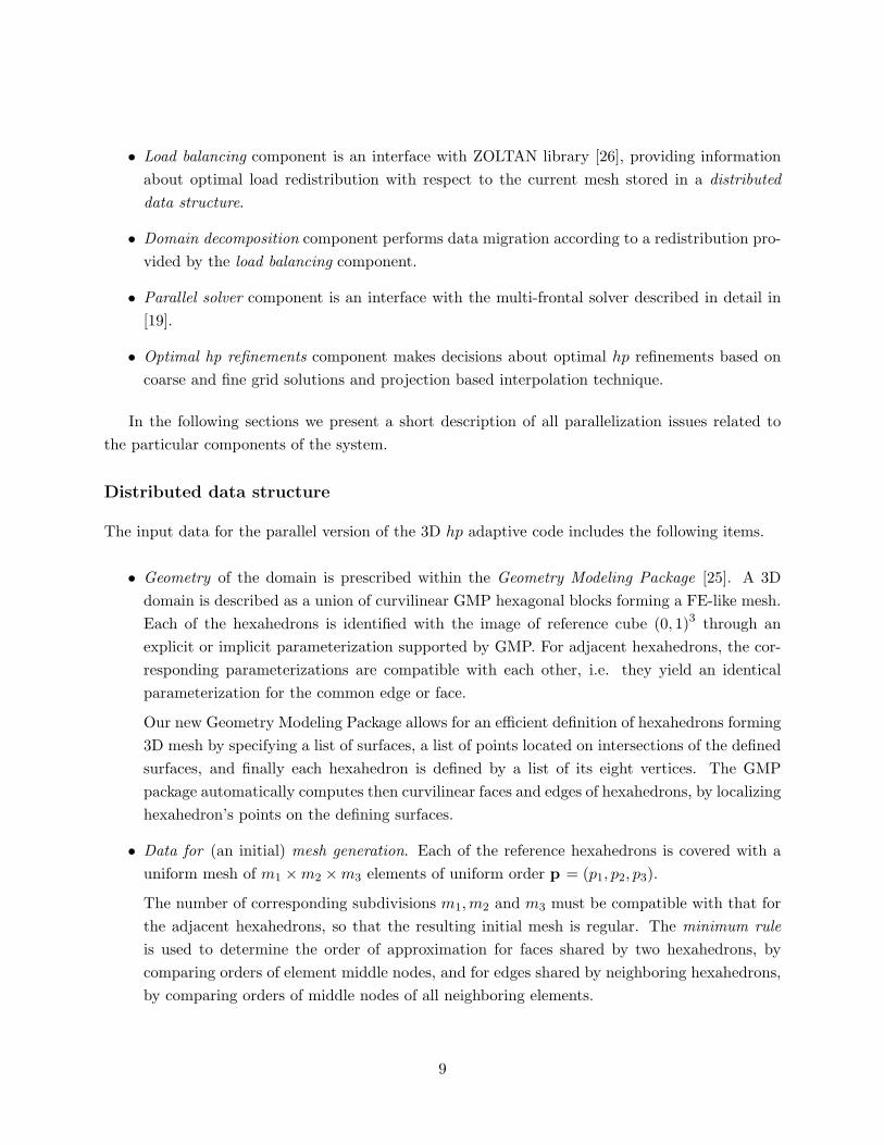
• Load balancing component is an interface with ZOLTAN library [26], providing information

about optimal load redistribution with respect to the current mesh stored in a distributed

data structure.

• Domain decomposition component performs data migration according to a redistribution pro-

vided by the load balancing component.

• Parallel solver component is an interface with the multi-frontal solver described in detail in

[19].

• Optimal hp refinements component makes decisions about optimal hp refinements based on

coarse and fine grid solutions and projection based interpolation technique.

In the following sections we present a short description of all parallelization issues related to

the particular components of the system.

Distributed data structure

The input data for the parallel version of the 3D hp adaptive code includes the following items.

• Geometry of the domain is prescribed within the Geometry Modeling Package [25]. A 3D

domain is described as a union of curvilinear GMP hexagonal blocks forming a FE-like mesh.

Each of the hexahedrons is identified with the image of reference cube (0, 1)3 through an

explicit or implicit parameterization supported by GMP. For adjacent hexahedrons, the cor-

responding parameterizations are compatible with each other, i.e. they yield an identical

parameterization for the common edge or face.

Our new Geometry Modeling Package allows for an efficient definition of hexahedrons forming

3D mesh by specifying a list of surfaces, a list of points located on intersections of the defined

surfaces, and finally each hexahedron is defined by a list of its eight vertices. The GMP

package automatically computes then curvilinear faces and edges of hexahedrons, by localizing

hexahedron’s points on the defining surfaces.

• Data for (an initial) mesh generation. Each of the reference hexahedrons is covered with a

uniform mesh of m1 × m2 × m3 elements of uniform order p = (p1, p2, p3).

The number of corresponding subdivisions m1, m2 and m3 must be compatible with that for

the adjacent hexahedrons, so that the resulting initial mesh is regular. The minimum rule

is used to determine the order of approximation for faces shared by two hexahedrons, by

comparing orders of element middle nodes, and for edges shared by neighboring hexahedrons,

by comparing orders of middle nodes of all neighboring elements.

9

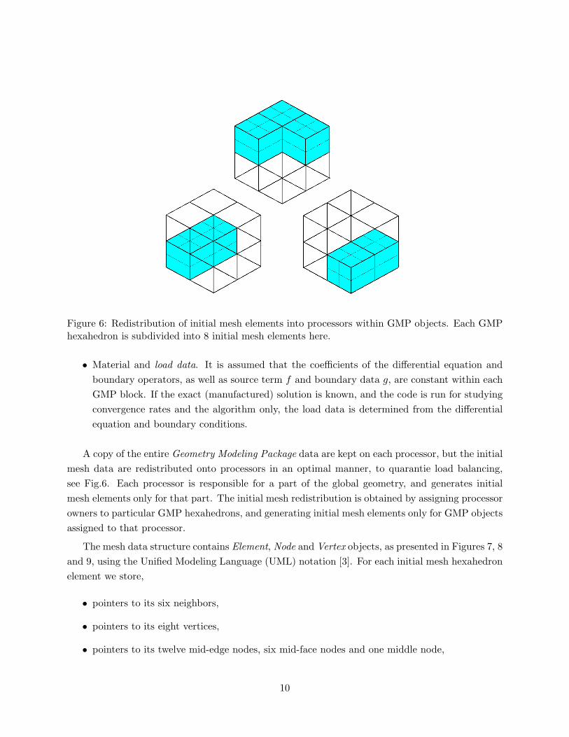
Figure 6: Redistribution of initial mesh elements into processors within GMP objects. Each GMPhexahedron is subdivided into 8 initial mesh elements here.

• Material and load data. It is assumed that the coefficients of the differential equation and

boundary operators, as well as source term f and boundary data g, are constant within each

GMP block. If the exact (manufactured) solution is known, and the code is run for studying

convergence rates and the algorithm only, the load data is determined from the differential

equation and boundary conditions.

A copy of the entire Geometry Modeling Package data are kept on each processor, but the initial

mesh data are redistributed onto processors in an optimal manner, to quarantie load balancing,

see Fig.6. Each processor is responsible for a part of the global geometry, and generates initial

mesh elements only for that part. The initial mesh redistribution is obtained by assigning processor

owners to particular GMP hexahedrons, and generating initial mesh elements only for GMP objects

assigned to that processor.

The mesh data structure contains Element, Node and Vertex objects, as presented in Figures 7, 8

and 9, using the Unified Modeling Language (UML) notation [3]. For each initial mesh hexahedron

element we store,

• pointers to its six neighbors,

• pointers to its eight vertices,

• pointers to its twelve mid-edge nodes, six mid-face nodes and one middle node,

10

Figure 7: Hexahedral initial mesh element object.

Figure 8: Refinement tree relations for a node object.

Figure 9: Refinement tree relations for a vertex object.

11

as presented in Fig. 7. Each GMP block stores one or more initial mesh elements.

When initial mesh elements are refined during hp adaptive iteration, element interior, faces and

edges are broken, and new nodes and vertices are created. We do not create new element objects.

Newly created nodes and vertices form refinement trees which grow from the initial mesh element

nodes.

A general structure of the refinement tree is presented in Figures 8 and 9. When a mid-edge

node is broken, two new mid-edge nodes and one vertex node are created. When a mid-face node

is broken in one direction (either horizontally or vertically), two new mid-face nodes and one mid-

edge node are created. When a mid-face node is broken in two directions (both horizontally and

vertically), four new mid-face nodes, four new mid-edge nodes and one new vertex are created.

When a middle node is broken in one direction, two new middle nodes and one mid-face node are

created. When a middle node is broken in two directions, four new middle nodes, four new mid-face

nodes and one new mid-edge node are created. When a middle node is broken in three directions,

eight new middle nodes, twelve new mid-face nodes, six new mid-edge nodes and one vertex node

are created. Each newly created node or vertex keeps a pointer to the father node. All nodes and

vertices of initial mesh element keep pointer to initial mesh element, since they don’t have a father

node.

During each stage of hp adaptive algorithm, the following mesh regularity rules are enforced

(compare [19]):

• A mesh, consisting of hexahedrons, is called regular, if the intersection of any two elements

in the mesh is either empty, reduces to a single vertex, or consists of a whole common edge

or a whole common face shared by the elements .

• An isotropic h-refinement occurs in 3D when an existing element is broken into eight son

elements.

• An anisotropic h-refinement occurs when an existing element is broken into either two son

elements in one of three possible directions, or four son elements in two of three possible

directions.

• An edge consists of two vertices and one mid-edge node. When an element is refined, in

isotropic or anisotropic manner, some of its edges are broken.

• A face consists of four vertices, four mid-edge nodes and one mid-face node. When an element

is refined, in isotropic or anisotropic manner, some of its faces are broken in an isotropic (four

son faces) or anisotropic (two son faces) way.

• During the isotropic h-refinement, an element is broken into eight smaller sons, as presented

in Fig.10. As a result of the refinement, a big element, shown in Fig.10 on the right-hand side,

12

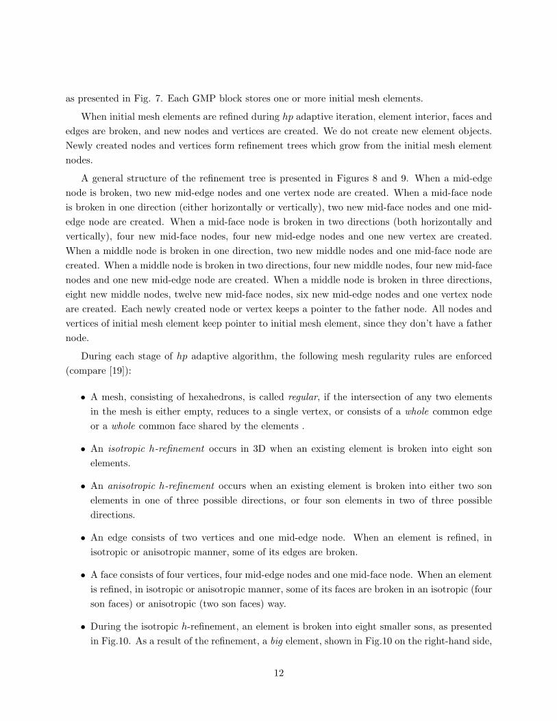
Figure 10: Isotropic refinement of a finite element. Mid-edge nodes and vertices of four newlycreated elements are called constrained nodes

has four smaller neighbors. In such a situation, twelve mid-edge nodes of smaller elements and

five common vertex of four smaller elements remain constrained with no new nodes generated.

The d.o.f. of constrained nodes are forced to match appropriate linear combinations of parent

nodes d.o.f in order to enforce the continuity of the approximation (hence the name) but they

do not exist in the data structure arrays.

• A mesh with constrained nodes is called an irregular mesh. It may happen that smaller

elements need to be broken once again, see Fig.11. In such a case newly created constrained

nodes are said to be multiply constrained.

• It is desirable for many reasons to avoid multiply constrained nodes, and limit ourselves to

1-irregular meshes only. We enforce this 1-irregularity rule by breaking only those elements,

which do not contain constrained nodes. In the case of hexahedrons, it is necessary to check if

any adjacent mid-face nodes are constrained. If a constrained node is found on some element

face, we must first break the neighboring element, as shown in Fig.12.

Load balancing

Load balancing is performed on the level of initial mesh elements via interfacing with the ZOLTAN

library [26].

For each initial mesh element identified by spatial coordinates of its centroid we provide ZOLTAN

with a load estimation based on the computational cost for element stiffness matrix integration.

13

Figure 11: Next refinement leads to the multiply constrained nodes

Figure 12: Enforcing breaking of neighboring elements, in order to enforce 1-irregularity rule

14

Having gathered this information from each processor, ZOLTAN employs one of its load balanc-

ing algorithms resulting in a new decomposition of the domain with the weights equally distributed

between sub-domains.

Data migration

All elements flagged by ZOLTAN to be exported to a neighboring sub-domain are packed into the

MPI buffer, and sent to the new destination sub-domain. The message scheduling is based on the

algorithm of coloring of graph representation for distributed computational domain [20].

After the data migration, each processor has two separated data structures: those elements

which have not been exported, and those elements which have been imported from neighboring

sub-domains. Each processor has now to merge those two data structures into a signle new data

structure.

The merging process consists of the following steps:

• Sorting elements according to spatial coordinates of their centroids.

• Merging data structures, one initial mesh element at a time.

• Identification of initial mesh elements neighbors using GMP.

• Reconnecting the new element to existing nodes.

• Addition of the remaining new nodes coming with the element.

• Reconstruction of refinement trees for the new nodes using the modified nodes numbering.

All elements from both data structures are sorted according to spatial coordinates of their centroids.

Such an order is required for the best performance of multifrontal solver. Elements from both data

structures are browsed in the above order. We add then one initial mesh element at a time, to the

new data structure.

First we identify newly added element neighbors already present in the new data structure. The

neighbors are identified by refering to GMP blocks. In order to connect the new element to existing

elements, we need to set neighbors pointer in the new element and in all the neighboring elements

already present in the new data structure. If the new element doesn’t have broken faces, we must

simply remove its face nodes on the connecting side, and connect the element to the face nodes of

the element already present in the data structure, as illustrated in Fig. 13. If the new element is

broken, we must remove its face on the connecting side together with their trees, and connect the

element to the broken face of the element already present in the data structure, see Fig. 14.

The last step of the merging algorithm consists in copying all other faces of the new element

eventually with refinement trees from old data structure to the new one. This must be done for

15

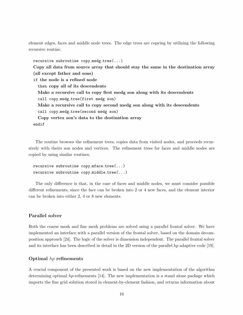
element edges, faces and middle node trees. The edge trees are copying by utilizing the following

recursive routine.

recursive subroutine copy medg tree(...)

Copy all data from source array that should stay the same in the destination array

(all except father and sons)

if the node is a refined node

then copy all of its descendents

Make a recursive call to copy first medg son along with its descendents

call copy medg tree(first medg son)

Make a recursive call to copy second medg son along with its descendents

call copy medg tree(second medg son)

Copy vertex son’s data to the destination array

endif

The routine browses the refinement trees, copies data from visited nodes, and proceeds recur-

sively with theirs son nodes and vertices. The refinement trees for faces and middle nodes are

copied by using similar routines.

recursive subroutine copy mface tree(...)

recursive subroutine copy middle tree(...)

The only difference is that, in the case of faces and middle nodes, we must consider possible

different refinements, since the face can be broken into 2 or 4 new faces, and the element interior

can be broken into either 2, 4 or 8 new elements.

Parallel solver

Both the coarse mesh and fine mesh problems are solved using a parallel frontal solver. We have

implemented an interface with a parallel version of the frontal solver, based on the domain decom-

position approach [24]. The logic of the solver is dimension independent. The parallel frontal solver

and its interface has been described in detail in the 2D version of the parallel hp adaptive code [19].

Optimal hp refinements

A crucial component of the presented work is based on the new implementation of the algorithm

determining optimal hp-refinements [14]. The new implementation is a stand alone package which

imports the fine grid solution stored in element-by-element fashion, and returns information about

16

Figure 13: Assembling of new unbroken element.

Figure 14: Assembling of new element broken into 4 element sons.

17

optimal hp-refinements in two stages. In the first stage, desired h-refinements flags are communi-

cated to the code. Upon performing the refinements and enforcing the 1 irregularity rule, the code

communicates back to the package the actual h refinements flags. In the final stage, the package

returns distribution of corresponding, optimal orders of approximation.

Except for a necessary communication between coarse grid edges, faces and elements, to deter-

mine maximum error decrease rates, the determination of optimal hp-refinements is a purely local

operation and, therefore, it is trivially parallellizable.

We summiarize now the algorithm in the following steps.

• Determining the optimal h refinements. Optimal h refinements decision is made for each

coarse grid element. Element can be broken in either one, two, or three directions. To

determine optimal h refinements for all edges, faces and elements, it is necessary to know

global maximum error decrease rates. The maximum rates can be computed by calling

MPI ALLREDUCE with MPI MAX parameter over all processors. This is the only need

for communication in that step.

• Performing the optimal h refinements. The h refinement decisions made in the previous step

are executed. The actual h refinements can be performed on each sub-domain in parallel, but

mesh 1-irregularity rule must be globally enforced.

• Determining the optimal orders of approximation for middle nodes. In this p refinement

process, a decision is made about optimal orders of approximation for element middle nodes.

The process is performed fully in parallel. The optimal hp refinement package sets optimal

orders of approximation for middle nodes only. Orders of approximation for faces and edges

are set during enforcing the minimum rule, discussed below.

• Setting the optimal orders for middle nodes. The p refinement decision made in the previous

step is executed. The process is fully parallel.

• Enforcing minimum rule. The order of approximation of each face is set to the minimum of

orders of middle nodes for all elements neighboring the face. Then the order of approxima-

tion for each edge is determined by taking minimum of orders of approximation of all faces

neighboring the edge. In order to enforce minimum rule for faces and edges located on the

interface between neighboring subdomains, we need to know orders of approximations from

elements adjacent to a current sub-domain, from all neighboring sub-domains.

In our 3D implementation of the parallel fully automatic hp adaptive code we have replaced the

mesh reconciliation algorithm developed for the 2D version of the code [19] with a new ghost

elements algorithm. The ghost elements are defined as an additional layer of elements adjacent

to a given sub-domain from neighboring subdomains. Elements adjacent to a sub-domain on

18

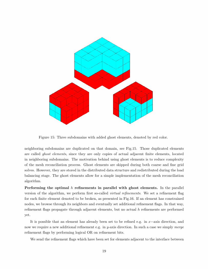
Figure 15: Three subdomains with added ghost elements, denoted by red color.

neighboring subdomains are duplicated on that domain, see Fig.15. Those duplicated elements

are called ghost elements, since they are only copies of actual adjacent finite elements, located

in neighboring subdomains. The motivation behind using ghost elements is to reduce complexity

of the mesh reconciliation process. Ghost elements are skipped during both coarse and fine grid

solves. However, they are stored in the distributed data structure and redistributed during the load

balancing stage. The ghost elements allow for a simple implementation of the mesh reconciliation

algorithm.

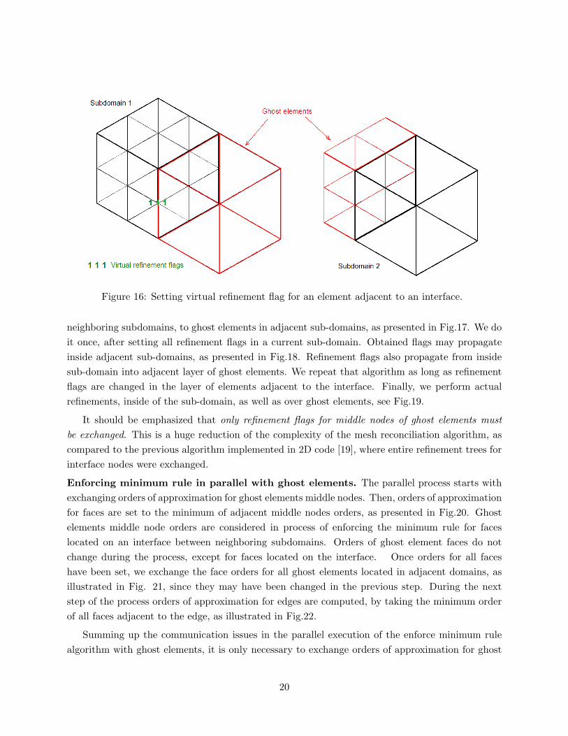
Performing the optimal h refinements in parallel with ghost elements. In the parallel

version of the algorithm, we perform first so-called virtual refinements. We set a refinement flag

for each finite element denoted to be broken, as presented in Fig.16. If an element has constrained

nodes, we browse through its neighbors and eventually set additional refinement flags. In that way,

refinement flags propagate through adjacent elements, but no actual h refinements are performed

yet.

It is possible that an element has already been set to be refined e.g. in x−axis direction, and

now we require a new additional refinement e.g. in y-axis direction. In such a case we simply merge

refinement flags by performing logical OR on refinement bits.

We send the refinement flags which have been set for elements adjacent to the interface between

19

Figure 16: Setting virtual refinement flag for an element adjacent to an interface.

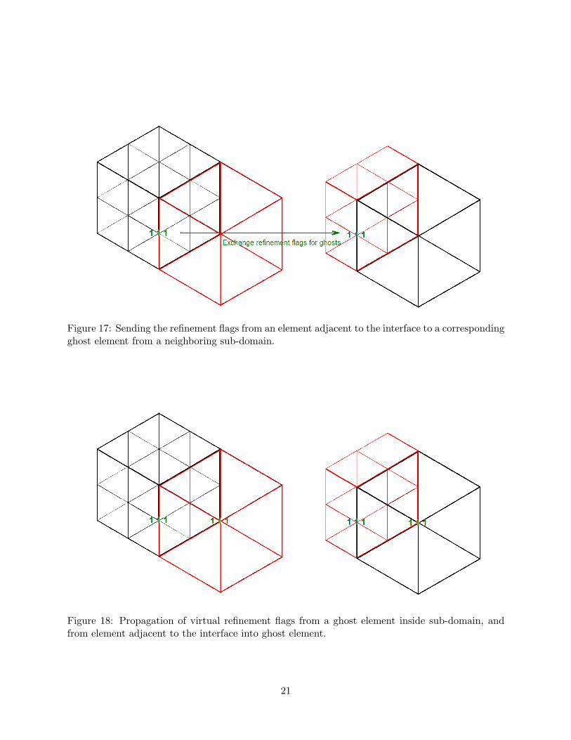
neighboring subdomains, to ghost elements in adjacent sub-domains, as presented in Fig.17. We do

it once, after setting all refinement flags in a current sub-domain. Obtained flags may propagate

inside adjacent sub-domains, as presented in Fig.18. Refinement flags also propagate from inside

sub-domain into adjacent layer of ghost elements. We repeat that algorithm as long as refinement

flags are changed in the layer of elements adjacent to the interface. Finally, we perform actual

refinements, inside of the sub-domain, as well as over ghost elements, see Fig.19.

It should be emphasized that only refinement flags for middle nodes of ghost elements must

be exchanged. This is a huge reduction of the complexity of the mesh reconciliation algorithm, as

compared to the previous algorithm implemented in 2D code [19], where entire refinement trees for

interface nodes were exchanged.

Enforcing minimum rule in parallel with ghost elements. The parallel process starts with

exchanging orders of approximation for ghost elements middle nodes. Then, orders of approximation

for faces are set to the minimum of adjacent middle nodes orders, as presented in Fig.20. Ghost

elements middle node orders are considered in process of enforcing the minimum rule for faces

located on an interface between neighboring subdomains. Orders of ghost element faces do not

change during the process, except for faces located on the interface. Once orders for all faces

have been set, we exchange the face orders for all ghost elements located in adjacent domains, as

illustrated in Fig. 21, since they may have been changed in the previous step. During the next

step of the process orders of approximation for edges are computed, by taking the minimum order

of all faces adjacent to the edge, as illustrated in Fig.22.

Summing up the communication issues in the parallel execution of the enforce minimum rule

algorithm with ghost elements, it is only necessary to exchange orders of approximation for ghost

20

Figure 17: Sending the refinement flags from an element adjacent to the interface to a correspondingghost element from a neighboring sub-domain.

Figure 18: Propagation of virtual refinement flags from a ghost element inside sub-domain, andfrom element adjacent to the interface into ghost element.

21

Figure 19: After performing actual refinements inside of sub-domain and over ghost elements.

Figure 20: Setting face orders by enforcing the minimum rule.

22

Figure 21: Exchanging orders for ghost elements faces.

Figure 22: Setting an edge order to the minimum of orders for faces adjacent to the edge.

23

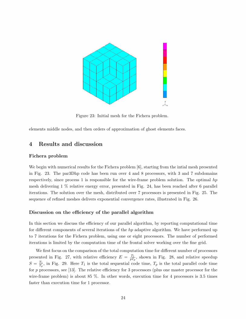
Figure 23: Initial mesh for the Fichera problem.

elements middle nodes, and then orders of approximation of ghost elements faces.

4 Results and discussion

Fichera problem

We begin with numerical results for the Fichera problem [6], starting from the intial mesh presented

in Fig. 23. The par3Dhp code has been run over 4 and 8 processors, with 3 and 7 subdomains

respectively, since process 1 is responsible for the wire-frame problem solution. The optimal hp

mesh delivering 1 % relative energy error, presented in Fig. 24, has been reached after 6 parallel

iterations. The solution over the mesh, distributed over 7 processors is presented in Fig. 25. The

sequence of refined meshes delivers exponential convergence rates, illustrated in Fig. 26.

Discussion on the efficiency of the parallel algorithm

In this section we discuss the efficiency of our parallel algorithm, by reporting computational time

for different components of several iterations of the hp adaptive algorithm. We have performed up

to 7 iterations for the Fichera problem, using one or eight processors. The number of performed

iterations is limited by the computation time of the frontal solver working over the fine grid.

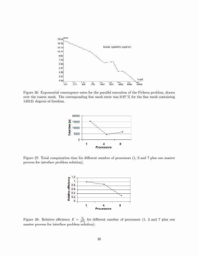
We first focus on the comparison of the total computation time for different number of processors

presented in Fig. 27, with relative efficiency E = T1

pTp

, shown in Fig. 28, and relative speedup

S = T1

Tp

, in Fig. 29. Here T1 is the total sequential code time, Tp is the total parallel code time

for p processors, see [13]. The relative efficiency for 3 processors (plus one master processor for the

wire-frame problem) is about 85 %. In other words, execution time for 4 processors is 3.5 times

faster than execution time for 1 processor.

24

Figure 24: Mesh redistribution into 7 processors, proposed by the ZOLTAN library.

Figure 25: The solution of the Fichera problem with 1 % energy error, distributed into 7 processors.

25

Figure 26: Exponential convergence rates for the parallel execution of the Fichera problem, drawnover the coarse mesh. The corresponding fine mesh error was 0.97 % for the fine mesh containing143121 degrees of freedom.

Figure 27: Total computation time for different number of processors (1, 3 and 7 plus one masterprocess for interface problem solution).

Figure 28: Relative efficiency E = T1

pTp

for different number of processors (1, 3 and 7 plus one

master process for interface problem solution).

26

Figure 29: Relative speedup S = T1

Tp

for different number of processors (1, 3 and 7 plus one master

process for interface problem solution).

Figure 30: Execution time for the most time consuming tasks of the code for the first five iterationson 4 processors.

27

Figure 31: Execution time for the most time consuming tasks of the code for the first six iterationson 8 processors.

28

Figure 32: Execution time for the components of the fine grid solve on 4 processors.

Figure 33: Execution time for the components of the fine grid solve on 8 processors.

29

Figure 34: Four initial mesh elements covering the central singularity.

The relative efficiency for 7 processors (plus one master processor) is about 30 % only. We

postulate that there are two reasons for the lost of the efficiency over the eight processors.

1. The sensitivity of the optimal hp refinements package to local differences between sequential

and parallel solver solutions of order 10−8 on the interfaces between neighboring subdomains.

2. Relation between working number of processors with number of singularities present in the

computational problem .

In order to support our conjectures, the following measurements have been performed.

We have measured the computation time for most time consuming steps of the parallel hp

adaptive algorithm, over each processor, as presented in Figures 30 and 31. These are the “coarse

grid solve”, where the parallel frontal solver is executed over the coarse mesh, “prepare to fine

grid solve” part, where some mesh consistency global operations are performed before the fine grid

solution, “fine grid solve”, “hp optimize” and “optimal hpref” steps responsible for parallel optimal

mesh refinements and reconciliation.

We have also measured the computation time for “forward elimination”, “backward substitu-

tion” and “interface problem solution” steps of the parallel solver solving the fine grid problem, for

each processor, and different number of processors, as reported in Figures 32 and 33. From these

measurements we can conclude that:

• The most time consuming step of the computations is the fine grid solution step, as it is

presented in Figures 30 and 31.

• The most time consuming step of the solver is the forward elimination step, as it is illustrated

in Figures 32 and 33, however the interface problem solution time grows quadritically with

the iteration number.

30

• Once the degrees-of-freedom corresponding to the fine grid solution, obtained from the parallel

solver differ from those obtained using the serial version of the code by 10−8 or more, the

resulting optimal meshes returned by the mesh optimization package start diverging from

each other.

• In order to get solution with energy greater then 36.785 on the coarse grid, we need to perform

6 iterations of the serial code, but only 5 iterations of the parallel code with 4 processors,

and again 6 iterations of the parallel code with 8 processors. Thus, we need to compare 6

iterations of the serial code with 5 iterations of the parallel code with 4 processors and 6

iterations of parallel code with 8 processors.

• The fine grid solution time for 8 processors is not well balanced, as presented in Fig. 33.

This is related to the number of initial mesh elements covering the singularities in the Fichera

problem, discussed in the next section.

Relation between number of processors and number of singularities

The load balance in our package is performed on the level of the initial mesh elements. As we have

showed in the analysis of our 2D parallel hp adaptive code [19], the number of processors should

be limited by the number of initial mesh elements covering singularities. In the Fichera problem,

there are only 4 initial mesh elements covering area with strongest singularities, as presented in

Fig. 34. Most of hp refinements in the Fichera problem are required in the neighborhood of this

area. This implies that the optimal load balance requires 4 processors only, since the overall load

over the rest of the domain becomes negligible after some initial iterations. Use of a larger number

of processors is not justified here.

Our numerical experiments indicate that we can resolve a point singularity with a 1 % accuracy

in our current implementation in a reasonable time. We believe that the possibility of resolving

singularities with 1 % accuracy in the same time will be extended to more complicated cases

provided the number of processors matches the number of singularities to be resolved.

5 Conclusion and Future Work

In the paper, a parallel version of the fully automatic 3D hp-adaptive FE method, has been pre-

sented. The three main technical challenges in parallelizing the sequential version of the code

included:

• mesh repartitioning accompanied by a regeneration of hp data structure arrays after each

mesh refinement, necessary to maintain load balancing,

• parallelization of a sequential (multi) frontal solver,

31

• parallel execution of optimal hp mesh refinements with global mesh regularity rules enforced

by means of ghost elements.

The par3Dhp package can be run on any parallel machine, equipped with Fortran 90 compiler, MPI

communication platform, and a C++ compiler, required for rebuilding the ZOLTAN library.

We have showed that parallel mesh refinements, mesh reconciliation and enforcement of the

minimum rule algorithms can be dramatically simplified with respect to those presented in 2D

version of the code, by using the concept of ghost elements. Moreover, ghost elements will also be

essential for a parallel implementation of the two grid solver [18], where the access to initial mesh

elements neighboring interfaces between domains is crucial.

The new implementation of the automatic optimal hp refinements package [14] allows for a

simple parallelization of the code. The package requires only three communications of maximum

energy for edges, faces and element middle nodes. The package is able to make decision about

optimal h refinements and orders of approximation for elements middle nodes locally, without any

excessive communication with neighboring domains. The optimal orders for faces and edges are set

by executing in parallel the minimum rule algorithm.

We have showed that the algorithm scales well for a reasonable number of processors, selected

with respect to the number of singularities detected in the computational domain. It follows from

the presented discussion that the use of large number of processors is motivated for problems with

a large number of singularities only.

We discuss now shortly our future work

• The current version of the parallel multi-frontal solver is relatively slow. We will switch to

MUMPS [17] parallel multi frontal solver, whose sequential version is 20 times faster then

sequential version of our current solver, according to our experiments.

• We would like to extend the code to be able to solve time-harmonic Maxwell equations, linear

elasticity and acoustics problems, and perform some massively parallel computations. The

scalability of our algorithm should be tested on some more complicated problems with larger

number of singularities then the Fichera model problem.

• We consider a parallelization of the two grid solver [18].

References

[1] A. Bajer, W. Rachowicz , T. Walsh, and L. Demkowicz, “A Two-Grid Parallel Solver for Time

Harmonic Maxwell’s Equations and hp Meshes”, Proceedings of Second European Conference

on Computational Mechanics, Cracow, Jun.25 - Jun.29, (2001).

32

[2] A. C. Bauer, A. K. Patra, “Robust and Efficient Domain Decomposition Preconditioners for

Adaptive hp Finite Element Approximations of Linear Elasticity with and without Discontin-

uous Coefficients”, International Journal for Numerical Methods in Engineering 59(3), (2004)

p.337-364

[3] G. Booch, J. Rumbaugh, I. Jacobson, The Unified Modeling Language User Guide Addison-

Wesley Professional, 1st edition (1998)

[4] J. D’Angelo, I. Mayergoyz, “Large-Scale Finite Element Scattering Analysis on Massively Par-

allel Computers”, Finite Element Software for Microwave Engineering, Eds. T. Itoh, G. Pelosi

and P.P. Silvester, Wiley & Sons, (1996)

[5] L. Demkowicz, “2D hp-Adaptive Finite Element Package (2Dhp90) Version 2.0”, TICAM Report

02-06 (2002)

[6] L. Demkowicz, D. Pardo, W. Rachowicz, “3D hp-Adaptive Finite Element Package (3Dhp90)

Version 2.0, The Ultimate (?) Data Structure for Three-Dimensionsl, Anisotropic hp Refine-

ments”, TICAM Report 02-24 (2002)

[7] L. Demkowicz, W. Rachowicz, and Ph. Devloo, ”A Fully Automatic hp-Adaptivity”, Journal

of Scientific Computing ; 17(1-3), p.127-155.

[8] L. Demkowicz, ”hp-Adaptive Finite Elements for Time-Harmonic Maxwell Equations”, Topics

in Computational Wave Propagation, Eds. M. Ainsworth, P. Davies, D. Duncan, P. Martin,

B. Rynne, Lecture Notes in Computational Science and Engineering, Springer Verlag, Berlin

(2003)

[9] L. Demkowicz, “Fully Automatic hp-Adaptivity for Maxwell’s Equations”, TICAM Report 03-

45, (2003).

[10] H. C. Edwards, “SIERRA Framework Version 3: Core Services Theory and Design.”

SAND2002-3616 Albuquerque, NM: Sandia National Laboratories, (2002)

[11] H. C. Edwards, J. R. Stewart, J. D. Zepper, “Mathematical Abstractions of the SIERRA

Computational Mechanics Framework.” Proceedings of the 5th World Congress Comp. Mech.,

Vienna Austria, (2002)

[12] H. C. Edwards, J. R. Stewart, “SIERRA, A Software Environment for Developing Complex

Multiphysics Applications.” Computational Fluid and Solid Mechanics Proc. First MIT Conf.,

Cambridge MA, (2001)

[13] I.Foster, Designing and Building Parallel Programs http://www-unix.mcs.anl.gov/dbpp/

33

[14] J. Kurtz, “Fully Automatic hp-Adaptivity for Acoustic and Electromagnetic Scattering in

Three Dimensions” (Ph.D. proposal), CAM Ph. D. Program, ICES, The University of Texas at

Austin, August 2005

[15] A. K. Patra, “Parallel HP Adaptive Finite Element Analysis for Viscous Incompressible Fluid

Problems” Dissertation University of Texas at Austin (1995)

[16] A. Laszloffy, J. Long, A. K. Patra, “Simple data management, scheduling and solution strate-

gies for managing the irregularities in parallel adaptive hp finite element simulations” Parallel

Computing 26, (2000) p.1765-1788.

[17] MUMPS: a MUltifrontal Massively Parallel sparse direct Solver,

http://www.enseeiht.fr/lima/apo/MUMPS/

[18] D. Pardo, L. Demkowicz, “Integration of hp-Adaptivity and Multigrid. I. A Two Grid Solver

for hp Finite Elements”, TICAM Report 02-33 (2002)

[19] M. Paszynski, J. Kurtz, L. Demkowicz, “Parallel Fully Automatic hp-Adaptive 2D Finite

Element Package”, ICES Report 04-07 (2004), accepted for publication in Computer Methods

in Applied Mechanics and Engineering

[20] M. Paszynski, K. Milfeld, “h-Relation Personalized Communication Strategy For HP-Adaptive

Computations”, TICAM Report 04-40 (2004) submitted to Concurrency and Computations,

Practise and Experience

[21] W. Rachowicz, D. Pardo, L. Demkowicz, “Fully Automatic hp-Adaptivity in Three Dimen-

sions”, ICES Report 04-22, accepted to Computer Methods in Applied Mechanics and Engineer-

ing

[22] J. F. Remacle, Xiangrong Li, M. S. Shephard, J. E. Flaherty “Anisotropic Adaptive Simulations

of Transient Flows using Discontinuous Galerkin Methods” Int. J. Numer. Meth. Engng. 00(1-

6), (2000)

[23] J. R. Stewart, H. C. Edwards, “ SIERRA Framework Version 3: h-Adaptivity Design and

Use.” SAND2002-4016 Albuquerque, NM: Sandia National Laboratories, (2002)

[24] T.Walsh, L. Demkowicz, “A Parallel Multifrontal Solver for hp-Adaptive Finite Elements”,

TICAM Report 99-01 (1999)

[25] Dong Xue, L. Demkowicz, “Geometrical Modeling Package. Version 2.0”, TICAM Report 02-30

(2002)

[26] “Zoltan: Data-Management Services for Parallel Applications”,

http://www.cs.sandia.gov/Zoltan/

34