PARALLEL IMPLEMENTATIONS OF HYPERSPECTRAL REMOTE SENSING ALGORITHMS A Thesis Presented by Cory James Crothers Brett to The Department of Electrical and Computer Engineering in partial fulfillment of the requirements for the degree of Master of Science in Electrical Engineering Northeastern University Boston, Massachusetts May 2014
Transcript
PARALLEL IMPLEMENTATIONS OF HYPERSPECTRALREMOTE SENSING ALGORITHMS
A Thesis Presented
by
Cory James Crothers Brett
to
The Department of Electrical and Computer Engineering
in partial fulfillment of the requirementsfor the degree of
This is the model for the total signal received by the sensor. From here, we need to make
some assumptions in preparation for the use of the detection algorithms. The first of them
being that the plume is optically thin. What this does is it gives an ability to say that τp(λ)
can be linearized. Next, the temperature difference between the background and plume
(∆T = Tp−Tb) must be small, so that we can linearize the Planck function. Finally, we use
a flat background emissivity approximation. This refers to the ability of the background to
radiate energy relative to a blackbody. This approximation will allow us to say that there
the emissivity is approximately one. With these approximations taken from [8], we get a
more workable signal model,
Lon(λ) =
Ng∑m=1
(Cb∆Tγm)τa(λ)αm(λ) + Loff(λ) (1.4)
where Cb is a constant. Up until this point, the model is the at-sensor model. So now, the
sensor needs to process that radiance, which adds some effects and noise, leading to
Lon(λ) = Lon(λ) ∗RF(λ) + η(λ) (1.5)
where η(λ) is noise added by the sensor, RF(λ) is sensors spectral response function, and
Lon is the radiance in the middle of the spectral channel λ. The operation ∗ is a convolution
10
operation. Renaming these and forming them into vectors,
x = Sg + v, v ∼ N(mb, Cb) (1.6)
where S is the gas signatures, g is linear mixture model coefficients, and v is the background
and noise clutter. This is the final signal model that we will use. Its simplicity is desired
because with this, we can now use mathematical techniques to complete our remote sensing
[8].
1.2.1 Signal Detection
Getting a good model for the image is important for formulating the detection algorithms.
Assuming that v ∼ N(mb,Cb), S to only have one signature, so S = s, and mb and Cb are
known by maximum likelihood test, we get a least-square solution,
g = (sTC−1b s)sTC−1
b x. (1.7)
The problem with g is that it is biased. By removing the mean mb, v will have new
distribution v ∼ N(0,Cb). Using Hypothesis testing,
H0 : g = 0 (Plume absent) (1.8)
H1 : g 6= 0 (Plume present) (1.9)
we can use the generalized likelihood ratio test approach [9], and get the MF detection
algorithm,
YMF =(xTC−1
b s)2
(sTC−1b s)−1
(1.10)
which then leads to the normalized matched filter (NMF)
YNMF =YMF
xTC−1b x
. (1.11)
The MF and NMF give a way to detect a chemical plume in HSI [8]. Graphical interpre-
tations of these derived detection algorithms can be just as informative and useful as the
11
mathematical derivations.
Figure 1.1: Example of a graphical approach
Figure 1.1 gives an insight into each pixel model. There are two Gaussian distributions
shown, the green being the background clutter, and the red pixels containing plume. Pixels
can fall between these if the pixel is made up of more than just plume.
Figure 1.2: Example of graphical approach: Demean
Removing the mean from the image is depicted in 1.2. It moves the background clutter
distribution to the origin as expected. It does not move the plumes distribution because
the mean is made up primarily of background clutter. In order to completely show how
YMF or YNMF are shown geometrically, the whitening must be represented in a figure.
12
Whitened space is a linear transformation converting variance of a distribution to 1.
In HSI, this means taking our data matrix X whose variance Cb and transforming it to
var(X) = ACbAT = σ2I. To express the derivation
Cb =1
np
XTX, (1.12)
we propose that using C− 1
2b can act as a whitening matrix, hence
Y = C− 1
2b X (1.13)
var(Y) = E[YYT ] = E[C− 1
2b X(C
− 12
b X)T ]
= E[C− 1
2b XXTC
−T2
b ] = C− 1
2b E[XXT ]C
−T2
b
= C− 1
2b CbC
−T2
b = I. (1.14)
This shows that Y is a whitened version of X. This whole system is not unique to C− 1
2b ,
but any rotation of that will work. For a more efficient way of getting a whitening matrix,
we use the Cholesky Decomposition. It breaks up Cb = LLT where L decomposes Cb into
upper and lower triangular matrices, and can be a whitening matrix. Using the cholesky
decomposition, we can do the same whitening technique. From here we can see the last and
final graphical representation
Figure 1.3: Example of graphical approach: Whitened
13
The whitening in Figure 1.3 is seen with the Gaussian distibutions. The shape has become
more circular which is evident by Cb = I. Now we can look at the decision boundaries for
the MF and NMF. The MF boundary is a plane that intersects the background and chemical
plume. We project each pixel onto the signature vector. If the projection crosses the MF
plane, then there is plume in that particular pixel. The NMF looks at the angle between the
signature vector and the pixel vectors. If the angle is small enough, then we say that there
is plume in that pixel.
Using these remote sensing algorithms, we will be able to detect different chemical gases
in an HSI image. We want to make these as fast as we can because if we are able to get the
data, process it before getting the next data cube, we could track chemical plumes in real
time. To implement this, we need to investigate different parallel computing architectures.
14
Chapter 2
Multicore CPU
Up until the early 2000s, most processors that were manufactured were single core processors.
At this point, processors hit fundamental limits and a redesign in technology was needed.
The first of these limits is the Power limit. As processors were given faster clocks, the
power was increasing. The processors were getting too hot, so there needed to be some way
to dissipate the power, and fans were not going to keep up. So, the performance of the
processor was limited by the amount of power that the computer could dissipate.
Next was the frequency limit. With the increase of instructions in pipelines, trying to
increase the functionality and throughput, there needed again to be a faster clock. But this
also came to a point where there were diminishing returns. Even if we added more steps to
the pipeline to account for different situations, the throughput would not increase because
there were too many steps.
Finally and most importantly, there is the memory limit. It has gotten to the point where
accessing DRAM memory is taking hundreds of cycles. Instead of the processor computing,
it is spending most of the time waiting for data to get to it. In single core processors, it is
the dominating factor in the processors performance [2].
Because of these fundamental limits in serial computing, the new design for processors
15
was a parallel, multicore design. This allowed for dividing tasks, and lowering the clock
speed. By lowering the clock speed, the power dissipation could remain maintained by fans.
They could now reduce the amount of steps in the pipeline because each core in the processor
did not need to work as hard. And each core has its own instruction cache and both can
send requests for data, so we will not be waiting as long for memory. The design started
with dual core processors, and has quickly escalated to more cores on a single processor chip.
2.1 Architecture
Architecture changes with different multicore processors. Depending on the company that
builds it, there will be some different aspects in each. For the most part, companies do not
release their actual design and pipelines for the public to see, but there is a general idea of
what the pipeline is doing. This along with memory organization will be explained below.
2.1.1 Processor
The processor as explained above has changed considerably since its creation. There has
been many advances in processor design, but it is based on the stages that are explained
below. For our purposes, explanation of things such as branch prediction or out of order
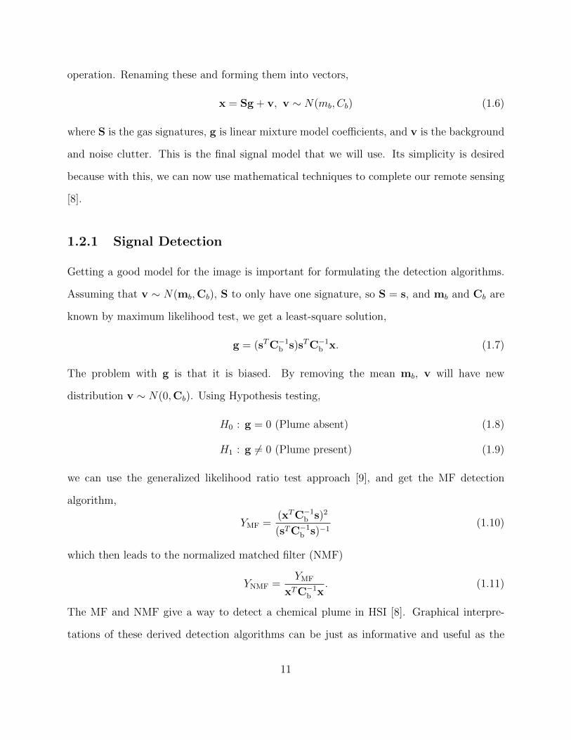
instructions is not necessary. Figure 2.1 is an example of a processor that one might find.
Explaining this form left to right, the first thing that should be noticed is the Fetch/Decode
control block. This attached to the instruction cache and instruction decoder. This is the
first stage of the pipeline; it grabs the next instruction from the instruction cache, and brings
it to the instruction decoder.
As shown, the instruction decoder (ID) is the next step. This is not only connected to the
instruction fetch (IF) stage, but also is connected to what is called the TLB. This stands for
translation look aside buffer (TLB). When an instruction is decoded, it has memory addresses
16
Figure 2.1: Example of CPU Architecture [1]
that it needs to access, but these addresses are in terms of virtual memory. Virtual memory
is used so that the processor thinks there is more memory than there actually is so it can
run many processes at once. Because of virtual memory we need to translate the virtual
memory address to the physical memory address, which is done on a page table. Page tables
will keep track of whether the page is located in the memory or disk as well as change a
virtual memory address to a physical one. The TLB is a full associative cache for the page
tables, following a least recently used replacement policy. The TLB will give the translation
very quickly, where as if the page table needs to be consulated that is not in the TLB will
cause a CPU stall. The decoder takes the instruction and turns it into something that the
load/store, and execution units can read.
Following the ID stage there are the execution units (EX). The EX stage takes the values
from the registers that were decoded in the ID stage, does the instruction to them and writes
them to an intermediate register.
Next is the memory stage (MEM), which takes the answer from the EX stage and gets
the memory location that it is going to be written to, then sends it to the write back (WB)
stage. This stage just writes the memory location to the new value.
17
Although there seems to be a lot more going on in Figure 2.1, most of the arrows are
just how each stage communicates with each other, and some blocks are just registers which
hold information and act as an intermediate step. This picture shows a generalized view of
what is going on with one core in a processor. So, in our case, we have multiples of these
cores running in parallel all with similar architectures shown in Figure 2.1. These cores are
hyperthreaded as well. Hyperthreading allows for two threads in each core, so two processes
can be running concurrently on one core [2]. All of the cores have separate L1 and L2 data
caches, and all are connected through the L3 data cache.
2.1.2 Memory
Memory hierarchy is arguably more important than what is going on in the processor. Al-
though it is improved with more cores in a single processor, the memory limitl does not go
away. Since memory is much slower than processors, a lot of the time processors are just
waiting for the data to get to them to complete the task the instruction has given. This still
happens with multicore processors, because the memory speed just cannot keep up with the
processor. It necessitates that we know how the memory is organized so that full advantage
of the processors speed can be taken. First, this is a general memory hierarchy picture,
Figure 2.2: Memory Pyramid [2]
This is just a basic general way to organize memory. First there are registers. These are
18
by far the fastest part of memory; they are used as intermediate steps in the pipeline, as
well as to store values that are used often. It would be advantageous for a programmer to
declare variables that are going to be used on a consistent basis as registers. As you can see,
it might only take three clock cycles to get from register to processor.
Our next best option is to have it in the L1 cache, L1 standing for level 1. This memory
is much bigger than the registers, on the order of 64Kb. It is the next place that a processor
will look for data, and if used efficiently, can prevent CPU stalls.
This pyramid in Figure 2.2 continues in this fashion, were the next best place for the data
to be is the next biggest memory type. The more amount of memory there is, the longer the
data will take to get to the processor. This leads to the first way we can optimize our code.
The closer we can keep the data to the processor, the better our code will perform. Even by
keeping the operation count the same, the best optimization a programmer can do is data
organization.
Now that we have established the hierarchy of the memory, there is some more design
organization that happens inside of a cache. There is three basic ways to organize a cache.
• Direct Mapped
• Set-way Associative
• Fully Associative
In direct mapped cache, each spot in the cache is associated with one memory location. It
means that only one memory location can exist in that cache location. This is the fastest way
and most efficient way to cache data, although it is not used in practice. Directed mapped
caches have complicated, expensive hardware, and take up a lot of space. For these reasons,
they are not used.
The next cache would be the fully associative cache. This cache is designed so that any
memory location can sit anywhere in the cache. A good thing about this is that we can
19
keep any combination of data in the cache. The problem is that as the cache grows in size,
the processor will take more time to find if the data sits in the cache, rendering the cache
useless. If a processor looks for a memory location in the cache, and cannot find it, it needs
to send a request for the memory location in the next memory stage. If it takes too long to
see if the value sits in the lower cache, then it would make more sense to go straight to the
higher cache.
Finally there is the Set-way Associative cache. This is by far the most popular design for
caches. It is a blend between direct mapped and fully associative cache. It basically means
that there are set locations in the cache that only certain memory can access, but a certain
memory location can be put in any of those locations.
Figure 2.3: 2-set way associative cache
Figure 2.3 shows a simplified cache scheme. In this example, there is only one cache and
there are 32 memory locations in the main memory. Memory locations 1-4 are red and are
associated with cache locations 1 and 2. This means that any of the red blocks can go into
20
the red cache locations, and nowhere else. So, the processor knows if it is requesting memory
locations 1-4, that it will first look in the first 2 cache locations, and if it is not there, it will
have to request the data from main memory. This gets the best of both worlds, in that the
cache is smaller, less expensive, and we can have combinations of memory in the cache.
2.2 Mapping Signal Detection to Multicore CPU
Hardware architecture is important to know so that when we are designing our code, we can
take full advantage of all the processor gives us. The software needs to be designed with the
hardware and memory hierarchy in mind, so that we can manipulate where the memory is,
and stop as many stalls as we can. It might seem that the software is more complicated, has
more for loops, or if statements. Concise code does not equate to performance.
2.2.1 Basic Linear Algebra Routines
Since there is a lot of linear algebra involved in our algorithms, the first thing that we looked
into was basic linear algebra routines (BLAS). These routines were developed in the 1980s
using FORTRAN in order to make linear algebra techniques available to engineers, which
eventually developed into MATLAB. Since then, there have been significant improvements not
only in processor power, but sophistication of BLAS routines. This lead to some investigation
on which BLAS routines we should use, and why is it the most effective.
It seemed that one BLAS library was beating all else. GotoBLAS is designed for perfor-
mance and compiled with hardware in mind. It uses all of the hardware mentioned above,
as well as some software optimization that makes it perform better. GotoBLAS gets a per-
formance boost when it considers the TLB in its design. By removing stalls from the TLB
misses, GotoBLAS can obtain maximum performance [10].
21
GEMM: Subroutine Optimization
GEMM is a term used in BLAS language. The GE stands for general, and MM is matrix
matrix multiply. Optimizing the GEMM routine will lend itself to all other BLAS routines,
and most important in HSI detection.
The discussion in this section is done with GotoBLAS design of GEMM. The open source
library that is used in this work is called OpenBLAS. OpenBLAS is an extension of GotoBLAS
and is an updated for newer CPU architectures. It is found here [11].
GEMM can be decomposed in many different ways. In our case, it is broken down in
steps as follows where C = AB + C. Notation is taken from [10].
Table 2.1: Dimensions of matrices
Matrix number of rows number of columns
A m k
B k n
C m n
Both A and B matrices can be decomposed into:
A =
(A0|A1|A2| . . . |Ak−1
)B =
B0
B1
B2
...
Bn−1
(2.1)
22
Consider that A0 is Rmxkc and B0 is Rkcxn. Next, this can be decomposed again
A0 =
A00
A01
A02
...
A0(m−1)
C =
C0
C1
C2
...
Cm−1
(2.2)
So our equation breakdown so far is
C0 = A00B0 (2.3)
Finaly, this meets its final smallest component:(C00|C01| . . . |C0(n−1)
)= A00
(B00|B01| . . . |B0(n−1)
)(2.4)
Assume that Aij is Rmcxkc , Bij is Rkcxnr , and Cij is Rmcxnr [10].
The reasoning behind breaking the matrix multiplication down into its smallest part is
because we need to find the best dimensions for our processor. Meaning we can now find out
the size of A00 that will fit inside the cache for fast access. Once A00 is no longer needed,
it will be copied back to main memory, and replaced by another sub matrix of A. We will
assume that Aij, Bij, and Cij will be able to fit inside the cache together, and that Aij will
be cached as long as it is needed.
In Section 2.1.2 we explain how the faster the memory, the smaller the amount of memory
that is available. So we need to decide where each sub matrix goes. If we count the amount of
memory operations, called memops, per floating point operations (FLOPs), we will see that
we need mckc memops from Aij, kcnr memops from Bij, mcnr memops from Cij reading,
mcnr memops from Cij writing. So we have mckc+(2mc+kc)n memops, and 2mckcn FLOPs.
Making an assumption kc << n [10]
2mckc2mc + kc
FLOPs
memops(2.5)
23
It is important to see because now we know that the bigger mckc, the more FLOPs we are
getting from the smaller amount of memops. If we look at this in terms of the dimensions
of Aij, the bigger Aij, the better. By putting Aij into the L2 cache, we are freeing space in
the L1 cache for Bij and Cij, as well as make Aij bigger.
The datas cache position is not the only important factor in organization. How Aij, Bij,
and Cij are organized in their respected cache will also affect performance. We will assume
that the data is in column major order. Moving data is generally done by accesses a group
of memory locations instead of one at a time. So, by packing Aij, Bij, and Cij into an
array that the processor will access contiguously, we can reduce the total number of memory
accesses.
Organizing the data in this way reduces the amount of cache misses, but they still occur.
The CPU can use techniques to mitigate these misses. The difference between a cache miss
and a TLB miss in terms of CPU response, is TLB misses will always cause a stall. To
mitigate TLB misses, pages have to be kept in the TLB for as long as they are needed and
then replaced, not only for fast translations [10].
We have found the dimension parameters for the sub matrices that fit into their respective
cache. Keep in mind that each core has its own L1 and L2 cache, so multiple parts of the
whole matrix can be computed independently. There was consideration put into the TLB and
its effect on performance, as well as the way the sub matrix is ordered in its respective cache.
The ability to do this data movement will have the biggest effect on overall performance of
each BLAS routine.
What is not seen in this memory optimization is the use of pthreads and SSE instructions.
pthreads is a primitive, low-level library that allows programmers to use multiple threads.
Many functions are built on top of pthreads for higher performance, including openMP,
which is used in our implementation. SSE instructions denotes Streaming SIMD Extensions
instructions. SIMD stands for Single Instruction Multiple Data. SSE takes multiple data
24
points, and does the same instruction on them at the same time. This cuts down on the
amount of instructions that need to be issued.
Figure 2.4: SSE example [3]
An example of how SSE instructions are used is shown in Figure 2.4. The registers are
actually 128 bits instead of just 64. This means we can fit 2 64 bit words into one register.
If we have two double precision numbers that have the same operation needed to be done
then we can cut down the time it takes to do both sequentially in half. Since linear algebra
is loaded with these types of instructions (multiply and add at many different memory
locations) SSE instructions are important to use when optimizing BLAS operations.
Since MF and NMF are highly linear algebra dependent, SSE instruction become a
crucial tool in the optimization process. Linear algebra is filled with just multiply and add
instructions on many data points, mapping perfectly to SSE.
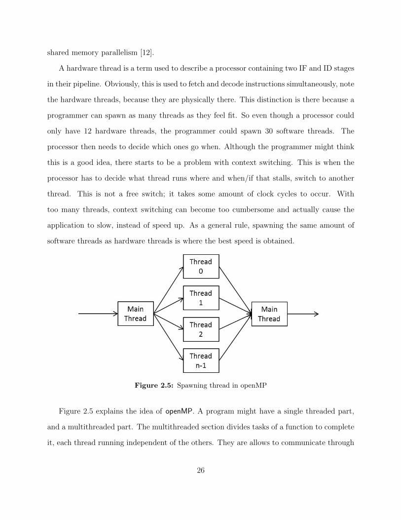
2.2.2 OpenMP
OpenBLAS is not the only open source library that was used in our implementations. Another
important one is openMP (open multiprocessor). This is an open source library that allows
for the use of multithreading. At openMP’s core, it is a set of library routines that express
25
shared memory parallelism [12].
A hardware thread is a term used to describe a processor containing two IF and ID stages
in their pipeline. Obviously, this is used to fetch and decode instructions simultaneously, note
the hardware threads, because they are physically there. This distinction is there because a
programmer can spawn as many threads as they feel fit. So even though a processor could
only have 12 hardware threads, the programmer could spawn 30 software threads. The
processor then needs to decide which ones go when. Although the programmer might think
this is a good idea, there starts to be a problem with context switching. This is when the
processor has to decide what thread runs where and when/if that stalls, switch to another
thread. This is not a free switch; it takes some amount of clock cycles to occur. With
too many threads, context switching can become too cumbersome and actually cause the
application to slow, instead of speed up. As a general rule, spawning the same amount of
software threads as hardware threads is where the best speed is obtained.
Figure 2.5: Spawning thread in openMP
Figure 2.5 explains the idea of openMP. A program might have a single threaded part,
and a multithreaded part. The multithreaded section divides tasks of a function to complete
it, each thread running independent of the others. They are allows to communicate through
26
data, but communication cuts into performance. Regardless of the hardware, openMP allows
to launch as many threads as desired, and the threads will map automatically to hardware.
openMP is a vital tool in our implementations of HSI algorithms. When appropriate, dividing
pixels into independent parts using openMP gives improvement in run time.
2.2.3 Summary
This chapter is really about utilizing all that the CPU gives us. The CPU gives us hyper
threading, so we take advantage of that. We get rid of CPU stalls as much as we can so the
processor can run unimpeded. We try and fit our matrices into packed forms so we can get
the data to the processor as fast as possible. None of this is possible without knowing not
only what is available to us in hardware, but the ins and outs of how it works together, and
take advantage of it.
27
Chapter 3
Graphics Processing Unit (GPU)
A GPU is a processor design for throughput and nothing else. It is not designed to have
many tasks to be running at once, or allow for internet connections, or run a word processor.
It is only there for mathematical operations. It was originally invented to process graphics
for video games. As video games became more popular, the GPU evolved for the growing
video gaming community. Because of its impressive throughput, it began to get the attention
of the scientific community for faster processing.
3.1 Architecture
The architecture of a GPU looks much different than that of a CPU. The design of a GPU
is for massive SIMD operations and impressive throughput. Figure 3.1 shows the basic
breakdown of the GPU as a whole. There is nothing special about the main memory and L2
cache as they work very similar to the main memory and L2 cache in the CPU. One thing
that you can notice from the very beginning is the amount of execution units compared to
Figure 2.1, where there is only a couple SSE execution units. The execution units dominate
the GPU where as it is a small portion in the CPU. This is because the CPU needs to be
28
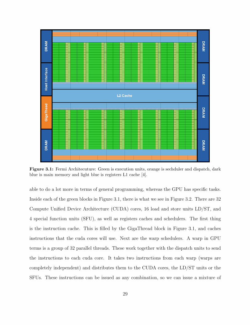
Figure 3.1: Fermi Architecuture: Green is execution units, orange is sechduler and dispatch, darkblue is main memory and light blue is registers L1 cache [4].
able to do a lot more in terms of general programming, whereas the GPU has specific tasks.
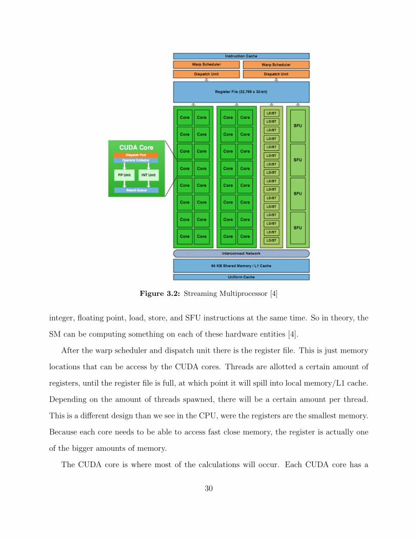
Inside each of the green blocks in Figure 3.1, there is what we see in Figure 3.2. There are 32
Compute Unified Device Architecture (CUDA) cores, 16 load and store units LD/ST, and
4 special function units (SFU), as well as registers caches and schedulers. The first thing
is the instruction cache. This is filled by the GigaThread block in Figure 3.1, and caches
instructions that the cuda cores will use. Next are the warp schedulers. A warp in GPU
terms is a group of 32 parallel threads. These work together with the dispatch units to send
the instructions to each cuda core. It takes two instructions from each warp (warps are
completely independent) and distributes them to the CUDA cores, the LD/ST units or the
SFUs. These instructions can be issued as any combination, so we can issue a mixture of
29
Figure 3.2: Streaming Multiprocessor [4]
integer, floating point, load, store, and SFU instructions at the same time. So in theory, the
SM can be computing something on each of these hardware entities [4].
After the warp scheduler and dispatch unit there is the register file. This is just memory
locations that can be access by the CUDA cores. Threads are allotted a certain amount of
registers, until the register file is full, at which point it will spill into local memory/L1 cache.
Depending on the amount of threads spawned, there will be a certain amount per thread.
This is a different design than we see in the CPU, were the registers are the smallest memory.
Because each core needs to be able to access fast close memory, the register is actually one
of the bigger amounts of memory.
The CUDA core is where most of the calculations will occur. Each CUDA core has a
30
floating point (FP) unit and integer (INT) unit, as well as another dispatch port. Each
CUDA core can run up to 48 threads at once, so each SM can handle 1536 threads. These
CUDA cores only have one task, and that is to compute the answer to whatever instruction is
given. Unlike the CPU, were its cores have to be able to do a multitude of tasks that general
computing will come up with, a CUDA core is doing multiplies and adds. An important piece
of information about each CUDA core is it contains a fused multiply add (FMA) instruction.
This means it will do c = a ∗ b+ d instructions without any rounding in between. This gives
a more accurate answer to the same equation on a CPU. Since linear algebra is loaded with
FMA instructions, we might get a more accurate answer than the CPU. So even though we
are doing the same calculation of both types of devices, we might get different answers, even
though both follow the IEEE standard. Finally there are the LD/ST units, which allow for
memory addresses to calculate for 16 threads in one clock cycle.
There is also another memory organization after the execution units seen in Figure 3.1.
This is a user configurable shared memory/L1 cache of 64Kb. The smallest each cache can
be is 16Kb. The L1 cache works exactly as the L1 cache explained in the CPU, and shared
memory will be explained in the next section.
There are 14 SMs in our Fermi GPU. As shown in Figures 3.2 and 3.1, the GPU is not
terribly complicated. It is evident that the GPU is designed with one thing in mind, and
that is throughput. To solve problems on a GPU, it is more efficient to use brute force
parallelism than it is to become clever in function design.
3.2 Running the GPU
The CPU and GPU are connected via PCI bus. In order for the GPU to run, the CPU
needs to send a command through its connection to start working. First thing that needs to
happen is to send the data over to the GPU. The PCIe2.0 supports up to 16Gb/s transfer,
31
which would be running at full capacity. So the CPU calls a memory transfer over to the
GPU, and this would be considered the first communication.
The memory transfer from CPU to GPU must happen, and needs to be factored in when
using the GPU. One thing that can be used to our advantage is the fact that the CPU and
GPU run asynchronously. This means that once the CPU calls a function to be run on the
GPU, it moves on to the next instruction. This will become an important in Section 3.3.
Although running asynchronously is the natural way the CPU and GPU work, we can also
change that to working synchronously. Function calls like cudaDeviceSynchronize() and
cudaMemcpy() will stall the CPU until the GPU completes that function. For our purposes,
having the GPU and CPU in sync does not help us because we cannot queue instructions,
as explained in Section 3.3.
Once the data is on the GPU we can start to use its functionality. It is hard to explain
the memory system and thread system separately so they will be explained together here.
Figure 3.3: Thread organization [4]
32
When a kernel starts to run, it has threads, blocks, and grids. A grid is a group of blocks
that share the same kernel. A block is a group of threads up to 1024 threads. The significance
of blocks is that each thread can communicate with each other in the block through shared
memory. Shared memory acts as a cache for a block. For example, suppose we have a vector
z of size n, and we run a kernel with n threads. During the kernel, every thread needs to
access every value in z. This would mean n2 main memory accesses. In the beginning of the
kernel, if we put all of z in shared memory, all of the thread could access every element in
z for a fraction of the memory cost of main memory. The second significant part of blocks
is that they run asynchronously. We do not have any control of what block is running when
on the GPU, so all blocks must be completely independent of all other blocks. Finally, a
thread can be thought of as an instance of a kernel. Each thread will do each instruction in
that kernel, similar to the threads on a CPU.
3.3 Mapping Signal Detection to GPU
The GPU has almost infinite amount of implementations of a single application. It can be
launched with many threads, small amount of threads, different amount of blocks in different
kernels, all run in the same kernel. There is a combination of these types of things that will
prove to be the best implementation of these algorithms. It is hard to find, and there must
be a lot of trial and error in order to find the best way to map our applications to the GPU.
First thing is to know what the software allows the programmer to utilize. When it comes
to the transfer of data, there isnt much that we can do, but what we can is important because
this is just overhead. There is no calculation occurring and we are just trying to get the data
from the CPU to the GPU, which can turn out to be a high percentage of the actual run time.
To get the data from CPU to GPU, there are two different function calls; one of them being
cudaMemcpy() and the second one being cudaMemcpyAsync(). During cudaMemcpy(), the
33
GPU will stall the CPU until the memory transfer is over. In cudaMemcpyAsync(), the GPU
will allow the CPU to move on to other calculations. In order to use cudaMemcpyAsync(), we
need to introduce streams. Streams are a sequence of operations that execute in issue-order
on the GPU [13]. The Fermi architecture allows for one compute stream, and two memory
transfer streams. It allows two memory transfer streams to allow for memory to be copied
to the GPU, while memory is being copied to the CPU. So, while we are copying some of
our data over to the GPU, we can start the detection process on previously transferred data.
Another memory optimization that we can take advantage of is called pinned memory.
When allocating memory on the CPU, we can flag it as pinned memory, which keeps the
pages for virtual to physical memory translation in the TLB. When this happens, the CPU
can access the data faster, and therefore transfer it over faster to the GPU.
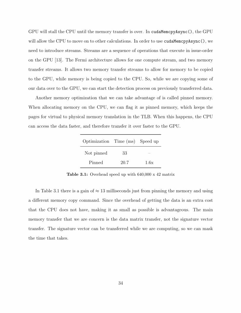
Optimization Time (ms) Speed up
Not pinned 33 –
Pinned 20.7 1.6x
Table 3.1: Overhead speed up with 640,000 x 42 matrix
In Table 3.1 there is a gain of ≈ 13 milliseconds just from pinning the memory and using
a different memory copy command. Since the overhead of getting the data is an extra cost
that the CPU does not have, making it as small as possible is advantageous. The main
memory transfer that we are concern is the data matrix transfer, not the signature vector
transfer. The signature vector can be transferred while we are computing, so we can mask
the time that takes.
34
Figure 3.4: Coalesce vs. Not coalesce memory accesses
In Figure 3.4 we see the difference between coalescing our memory reads and not coa-
lescing our memory reads. The left most part of Figure 3.4 is coalescing and the right is
the opposite. The way that memory is accessed on a GPU is in chunks. For example, if a
thread wants to access a global memory location called q for discussion purposes, a group
of memory locations around q are brought with it. So if we coalesce our memory reads we
will minimize the amount of global memory accesses since the locations around that one
accessed are already cached. If we do not coalesce our memory reads, each thread will need
to grab a chunk of memory, since it cannot rely on the fact that the thread next to it had
already grabbed its memory location. Accessing global memory can be expensive in terms
of clock cycles, so by minimizing these accesses, we will speed up our kernels. To Illustrate
this, there is a study done by NVIDIA whereby the make a kernel to just read floating point
numbers. One is done by with coalesce memory reads, and the other is done without them.
The results are in [13].
35
Table 3.2: NIVIDA study by Paulius Micikevicius
Coalesced Timing (µs) Speed up
Yes 356 –
No 3,494 ≈ 10x
Just by changing the way you access memory on the GPU can change the timing for such
a simple operation. This study was done with 12 Mb of data, where as we have on the order
of 100 Mb of data. Since we have more data, coalesce reads becomes more important.
3.3.1 cuBLAS and MAGMA
cuBLAS and Matrix Algebra on GPU and Multicore Architectures (MAGMA) are the basis
libraries for linear algebra on the GPU. We need both because cuBLAS does not contain
some important linpack matrix decompositions that we need for detection. What cuBLAS
does not have MAGMA makes up for. The highest FLOPs that cuBLAS gets is with square
matrices, where as in MAGMA, there is multiple designs for each routine. Since there is
so many ways to optimize GPU code, different thread and block and even different kernel
design can make a big difference in performance. By using both of these libraries, we can
tune our application to the fastest code, depending on the dimensions of our cube.
For example, lets look at the matrix-vector multiplication on a GPU. We will look at
four different situations that will necessitate different threads and blocks, and what each
thread is doing. First, we will look at ”tall and skinny” matrices. These types of matrices
will benefit from one thread per row implementation of matrix-vectors multiplication. Since
there are 14 SMs in a Fermi GPU card, and each SM can handle 1536 active threads, so
that is 1536 · 14 = 21504 rows of a matrix that can be multiplied by a vector at once.
Since every thread in each block needs to access the vector x in Ax = y we will put it in
36
shared memory for each block so every thread can access it quickly. We will accumulate the
products in a register for each thread because this is the fastest type of memory. Once we
have the dot product, we will put the register in the correct memory location of y. Next, for
more square matrices, the best performance comes from a several threads per row design.
This breaks the blocks into two-dimensions, meaning each thread has an x and y direction
identification. Each block will serve a sub matrix of A and a sub vector of x. Again we will
put the sub vector into shared memory for easy access. We will now need to introduce the
atomicAdd() functionality of the GPU. Atomic functions allow all threads to sum a value
in global memory. This can occur with threads from different blocks. For the sum to be
correct, the GPU only allows one thread to access the memory location at once. Once it is
completed another thread can access it and so on. Although this will cause threads to be
waiting for the opportunity to access the memory location, it is a better option than making
another kernel to sum these partial values, which is the only other option. We can then
have several rows per thread. If a matrix is very tall and skinny, on the order of hundreds of
thousands of rows and small amount of columns, this will be the fastest implementation. It
will minimize the shared memory accesses since we will be holding a lot of data in registers.
There is one more but it does not need to be discussed for our applications. It is clear that
because of our situation with our data cubes in general, we will benefit from the several rows
per thread optimization [14].
We have looked at the macro side of the matrix vector case; we can now switch gears and
look at the inner workings of a general matrix multiplication GEMM. GEMM is the biggest
operation that we have in our application, so in the same situation as the CPU, optimizing
this is our biggest priority.
The GPU works much better with independent calculations. The blocking system has
been designed in GEMM so that each block does not need to talk to another block and
therefore speed up our application. So if we can manipulate C = AB + C, into independent
37
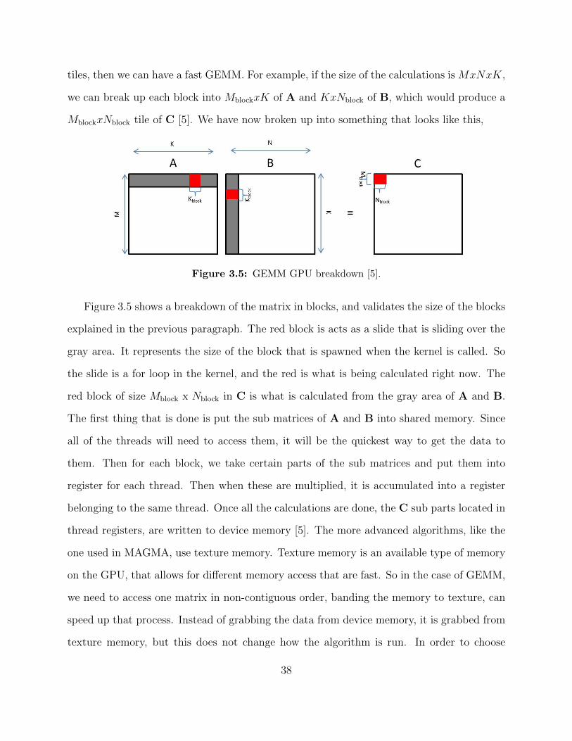
tiles, then we can have a fast GEMM. For example, if the size of the calculations is MxNxK,
we can break up each block into MblockxK of A and KxNblock of B, which would produce a
MblockxNblock tile of C [5]. We have now broken up into something that looks like this,
Figure 3.5: GEMM GPU breakdown [5].
Figure 3.5 shows a breakdown of the matrix in blocks, and validates the size of the blocks
explained in the previous paragraph. The red block is acts as a slide that is sliding over the
gray area. It represents the size of the block that is spawned when the kernel is called. So
the slide is a for loop in the kernel, and the red is what is being calculated right now. The
red block of size Mblock x Nblock in C is what is calculated from the gray area of A and B.
The first thing that is done is put the sub matrices of A and B into shared memory. Since
all of the threads will need to access them, it will be the quickest way to get the data to
them. Then for each block, we take certain parts of the sub matrices and put them into
register for each thread. Then when these are multiplied, it is accumulated into a register
belonging to the same thread. Once all the calculations are done, the C sub parts located in
thread registers, are written to device memory [5]. The more advanced algorithms, like the
one used in MAGMA, use texture memory. Texture memory is an available type of memory
on the GPU, that allows for different memory access that are fast. So in the case of GEMM,
we need to access one matrix in non-contiguous order, banding the memory to texture, can
speed up that process. Instead of grabbing the data from device memory, it is grabbed from
texture memory, but this does not change how the algorithm is run. In order to choose
38
what the dimensions of the sub matrices will be, Mblock, Nblock, andKblock, we need to take
in consider some GPU hardware specifications.
1. warp size
2. threads per block
3. registers per thread
4. shared memory size.
We care about the warp size because this will define how many threads can be scheduled at
once. And keeping the amount of threads in a block as a multiple of warp size can improve
performance. The amount of threads per block is also important because it will help define
the size of the sub matrices of A and B. We care about how many registers per thread
because this will be a big limitting factor in the size that Mblock and Nblock can be. If we
use too many registers, they spill into what is called local memory. The name is deceiving
because local memory resides in global memory, the slowest of all memories. Although this is
mitigated by the emergence of L1 cache in Fermi architecture, it is bad GPU coding practice
to spill registers. Using these guidelines, the GEMM function is tuned to our GPU, and
performed at its highest performance.
3.4 Summary
Using these techniques, libraries, and hardware, we can create high throughput algorithms
on the GPU. Although the GPU and CPU are different in architecture, algorithm design,
fundamental optimizations, the idea is still the same; take what the device give you. Design
the application around the hardware, and taking everything into account. The more that
you can consider and weave into the application design, the faster the application will be.
There needs to be a fundamental understanding on what is going on in the hardware, as
much as software says you do not, in order to create optimized code.
39
Chapter 4
Matched Filter
This chapter will explain how we break down the MF algorithm for an efficient implementa-
tion. As explained in the Section 1.2, we get the algorithm from assumptions that are used
to make this problem doable. We will define the algorithm itself, how it is done on the CPU
and GPU, and where the designs change due to hardware. We will also go into what else
could be done to improve the performance.
4.1 Algorithm
The Matched filter, Equation 1.10 can be broken down into five different components. Al-
though these components vary in number of operations and complexity, any naively imple-
mented component will greatly diminish the overall performance.
Figure 4.1: Matched-filter (MF) and Normalized Match-filter (NMF) components
Figure 4.1 shows a block diagram for both the MF and NMF. For this explanation, the
reader needs to know that the data matrix Xb is Rnpxnb where nb is number of bands, np is
40
number of pixels, and u =
[1 . . . 1
]Tand is contained by Rnpx1
mb =1
np
·XTb u (4.1)
First we must find the mean of each band so that we can demean our data.
X0 = Xb − umTb (4.2)
Now that the data is demeaned, we can calculate the covariance,
Σ =1
np
·XT0 X0. (4.3)
As seen in Figure 4.1 the next step will be to whiten the data. Whitening of data can
be performed by and any matrix A such that AΣAT = σ2I where σ2 is arbitrary [15].
Usually, this is done by Σ− 12 , but this is not necessary. Since inverting a whole matrix is
very expensive, we use the Cholesky decomposition which is discussed in detail in Section
1.2.1,
Σ = LLT (4.4)
where L−1 is a whitening matrix.
Xw = X0L−1 sw = L−1s (4.5)
Since we have whitened data, the equation 1.10 can reduce to,
ymf =1
sTwsw
· (Xwsw) . ∗ (Xwsw). (4.6)
This is the extent of the algorithm when it is broken down into parts. At first glance,
the thought is that we will only need BLAS for the covariance computation, the Cholesky
decomposition and the whitening steps. This is where the most computation occurs in MF
so reducing this time will give us the best run time. We can also get some more performance
out of some not so obvious tasks. Equation 4.1 and 4.2 are set up in a way that leads to
explore BLAS routines. To give a summary of the algorithm floating point operations in the
41
same type of break down,
Table 4.1: gflops per instruction
Function gFLOP count CPU gFLOP count GPU
Mean .01064 .01064
Mean Subtract .01056 .01056
Covariance .6868 1.363
Whitening .00075 .00075
Matched Filter Scores .01069 .0169
Total gflop .719564 1.3959
These FLOP counts in Table 4.1 are found in [16]. The FLOP count for the GPU and the
CPU are different because we use different BLAS functions for the covariance computation.
The way to get performance on a GPU and a CPU are different. On a CPU, by minimizing
the FLOP count and having an intelligent function design will yield the best implementation.
On a GPU, by using more brute force meaning every thread doing the same thing, and every
keeping functions simple yield the best performance. This is evident by the FLOP count
on the CPU and GPU. Instead of having threads turning on and off to reduce the FLOP
count on a GPU, we have all threads doing the same calculation. The real difference is in
the covariance computation. On the CPU, we only calculate half of the covariance since it is
a semi-definite symmetric matrix, whereas on the GPU, we calculate the whole covariance.
4.2 Results
The results of the MF algorithm were performed on both a multicore CPU and a GPU. The
CPU is an Intel(R) Xeon(R) X5650 processor. It runs at 2.66 GHz, has six cores, and twelve
42
hardware threads. The total amount of on chip cache is 12 Mb.
The GPU used is a Tesla C2050 graphics card. It contains 3Gb of main memory, con-
figurable 64Kb of shared/L1 cache memory. It has 448 CUDA cores each running at 1.15
GHz.
All results are optimized for a sensor that gives images of size np = 40960 and nb = 129.
All GPU functions are optimized for this configuration, and will need to be changed for
different sizes.
4.2.1 Mean and Mean Subtraction
Mean and mean subtraction might seem like simple calculations. The do not require many
computations and can be implemented easily with for loops. To illustrate the importance of
speeding even the smallest components up, we can look at the three implementations shown
below.
Table 4.2: Timing of various mean-computation methods on the CPU
Method Time Speedup
For Loop 5.8ms 1.0x
openMP 4.1ms 1.4x
OpenBLAS 1.1ms 5.2x
You can see that we can save 4.7 ms by changing the mean calculation from a naive for
loop to using OpenBLAS. openMP also gives some type of speed up but not to the extent
of OpenBLAS which uses all of the optimizations explained in 2.1. This shows the power of
data organization. There is not much of a difference in the number of FLOPs, but the data
management, multithreading and SSE instructions allow for 5.2x speed up.
The same thing can be said about the 4.2 equation. By changing it to a matrix rank-1
43
update, where u and mb create a matrix, which is then subtracted from Xb, save us more
time. It solidifies the fact that it is not the speed of the processor, it is the optimization
techniques dicussed in 2.1.
On the GPU, the process of working to get efficient implementations of 4.1 and 4.2 is dif-
ferent. When looking at these equations, set up in linear algebra fashion, our initial thought
is to send the data over to the processor, and then do two BLAS routines, cublasSgemv()
and cublasSger(). These are a matrix vector multiplication and a rank-1 update of the
data matrix. Looking at the timeline produced by Nsight, a GPU profiler,
Figure 4.2: cuBLAS implementation of Equations 4.1 and 4.2.
In Figure 4.2, we can see the breakdown of timing with the memory transfer, cublasSgemv()
and cublasSger(). Knowing about streams from Section 3.3 we can see that we are not
utilizing the compute stream while data is being transferred. Since computing the mean for
each band is completely independent, we can send over bands separately. This would allow
us to overlap the memory transfer and computations. So we decided to stream some of the
data, start calculating the mean, while more of the data is being transferred over. The first
thought was to transfer it in a band at a time, compute the mean of that band using shared
memory with a decomposition technique in [6]. This summation technique is graphically
explained below.
44
Figure 4.3: Technique in [6]. One block of many launched
The vectors are contained in shared memory. Each iteration we are cutting the number
of calculations in half. To map this to our data, we use the np threads. We cannot put
that many threads into one block, so multiple blocks are also used. We put a section of the
spectral band into each blocks shared memory, and sum that section with design ??. Once
the sum is calculated, each block uses the atomicAdd() function to sum and get the mean
of the spectral band. This was run with 8 streams, sending one spectral band at a time.
Figure 4.4: First Memory Overlap attempt. 256 threads and 160 blocks were spawned
45
This did not work very well. We were able to overlap some of the transfers, but it seems
to be very scattered. Also the kernel itself is taking longer than the memory copy. To be
completely efficient we want the kernel to be at most as big as every transfer, so that we
can completely overlap them without any extra time. So, we decided to look at the kernel.
With this kernel design, we need to rely heavily on shared memory. This is not necessarily
a bad thing, but it somehow we could get it into registers, the faster the kernel would run.
So instead of using np threads, we use less threads. This allows us to use coalesce memory
reads and make partial sums in each thread. From there, each thread puts its partial sum
into shared memory. Now, we have a vector of partial sums in shared memory. From here,
we use the same summation technique seen in Figure ??.
Figure 4.5: Second memory overlap attempt. 256 threads and 20 blocks were spawned
One thing to notice is that we are using 140 less blocks, so 140 ∗ 256 = 35840 threads
that we are not using anymore, but the speed of the kernel is faster. It is just another
example on the GPU that we do not want to just have as many threads as we can, and
putting some more thought into the memory systems, the faster the kernel can be. We again
can optimize this even more. Notice that in Stream 12, Stream 13, and Stream 19, we do
not have overlapping. Consulting [13], the ordering of when the kernels are called matters.
46
We want to fill the compute and transfer stream queues before moving on to the next one
respectively. So, instead of calling a memcpyAsync() followed by computeMean() kernel, we
called all the memcpyAsync()s followed by all of the computeMean() kernels.
Figure 4.6: Third memory overlap attempt. 256 threads and 20 blocks were spawned
Now, looking at Figure 4.6 we can see we are overlapping to the best of our ability. This
is after an initial startup, and more toward the middle of the for loop. This still was not
as good as the BLAS operations, and we have not implemented the mean subtraction yet,
but it seems that this is the way to go. Since there are many ways to complete this task, we
decided to look at a different approach. This was to send over many bands at a time, to get
a bigger transfer, and then spawning a block per band, and using coalesce memory reads,
and getting rid of the shared memory aspect of our kernel. Now we just accumulate pixels in
threads, and then use atomic functions to add all of those values. The block spawned take
care of the spectral bands sent over depicted below.
47
Figure 4.7: Mean Algorithm
Each block is assigned to one spectral band, and threads accumulate pixels in a coalesce
fashion. Once all of the pixels have been added to their respected thread in a block, then
we use atomic functions to sum all partial sums that each thread contains. So we send the
data over in thirds, and add in the mean subtract.
Figure 4.8: Fourth memory overlap attempt. 256 threads and 43 blocks were spawned
Finally putting everything together, meaning adding some more streams, and making
the kernels overlap as best as possible.
48
Figure 4.9: Fifth memory overlap attempt. 256 threads and 16-17 blocks were spawned
Table 4.3: Timing attempts for initial data copy
Method Time Speedup
cuBLAS 6.38 ms –
Attempt 1 10.25 ms .62x
Attempt 2 6.07 ms 1.05x
Attempt 3 5.68 ms 1.12x
Attempt 4 5.63 ms 1.13x
Attempt 5 5.18 ms 1.23x
Our final implementation has saved us≈ 1 ms from our total GPU implementation. When
trying to squeeze out all of the performance that we can, this is the type of exploration that
is needed.
4.2.2 Covariance
The covariance computation is what dominates all of the calculations for the MF. It is a third
order BLAS operation with the highest FLOP count. It was very clear from the beginning
49
that BLAS was going to be needed for this calculation because of the amount of optimization
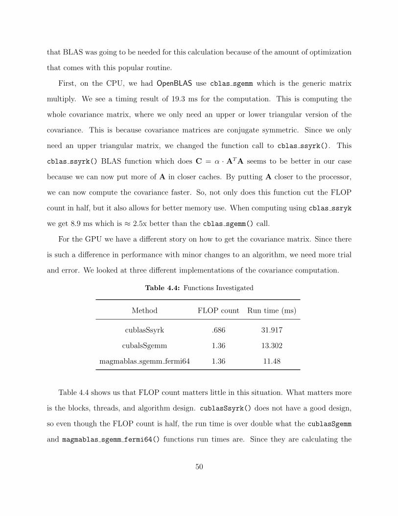
that comes with this popular routine.
First, on the CPU, we had OpenBLAS use cblas sgemm which is the generic matrix
multiply. We see a timing result of 19.3 ms for the computation. This is computing the
whole covariance matrix, where we only need an upper or lower triangular version of the
covariance. This is because covariance matrices are conjugate symmetric. Since we only
need an upper triangular matrix, we changed the function call to cblas ssyrk(). This
cblas ssyrk() BLAS function which does C = α · ATA seems to be better in our case
because we can now put more of A in closer caches. By putting A closer to the processor,
we can now compute the covariance faster. So, not only does this function cut the FLOP
count in half, but it also allows for better memory use. When computing using cblas ssryk
we get 8.9 ms which is ≈ 2.5x better than the cblas sgemm() call.
For the GPU we have a different story on how to get the covariance matrix. Since there
is such a difference in performance with minor changes to an algorithm, we need more trial
and error. We looked at three different implementations of the covariance computation.
Table 4.4: Functions Investigated
Method FLOP count Run time (ms)
cublasSsyrk .686 31.917
cubalsSgemm 1.36 13.302
magmablas sgemm fermi64 1.36 11.48
Table 4.4 shows us that FLOP count matters little in this situation. What matters more
is the blocks, threads, and algorithm design. cublasSsyrk() does not have a good design,
so even though the FLOP count is half, the run time is over double what the cublasSgemm
and magmablas sgemm fermi64() functions run times are. Since they are calculating the
50
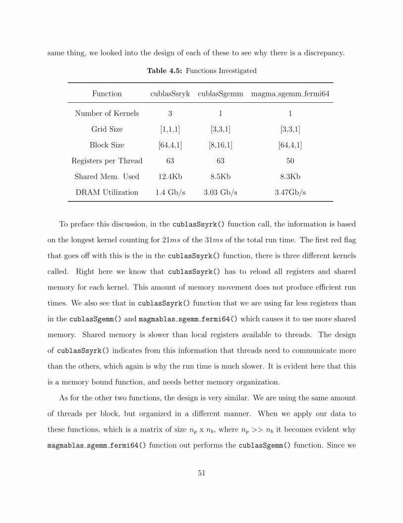
same thing, we looked into the design of each of these to see why there is a discrepancy.
Table 4.5: Functions Investigated
Function cublasSsryk cublasSgemm magma sgemm fermi64
Number of Kernels 3 1 1
Grid Size [1,1,1] [3,3,1] [3,3,1]
Block Size [64,4,1] [8,16,1] [64,4,1]
Registers per Thread 63 63 50
Shared Mem. Used 12.4Kb 8.5Kb 8.3Kb
DRAM Utilization 1.4 Gb/s 3.03 Gb/s 3.47Gb/s
To preface this discussion, in the cublasSsyrk() function call, the information is based
on the longest kernel counting for 21ms of the 31ms of the total run time. The first red flag
that goes off with this is the in the cublasSsyrk() function, there is three different kernels
called. Right here we know that cublasSsyrk() has to reload all registers and shared
memory for each kernel. This amount of memory movement does not produce efficient run
times. We also see that in cublasSsyrk() function that we are using far less registers than
in the cublasSgemm() and magmablas sgemm fermi64() which causes it to use more shared
memory. Shared memory is slower than local registers available to threads. The design
of cublasSsyrk() indicates from this information that threads need to communicate more
than the others, which again is why the run time is much slower. It is evident here that this
is a memory bound function, and needs better memory organization.
As for the other two functions, the design is very similar. We are using the same amount
of threads per block, but organized in a different manner. When we apply our data to
these functions, which is a matrix of size np x nb, where np >> nb it becomes evident why
magmablas sgemm fermi64() function out performs the cublasSgemm() function. Since we
51
are launching [64, 4, 1] threads per block, and the nature of our data being a tall skinny
matrix, the threads map better for memory access in the [64,4,1] pattern than the [8,16,1]
pattern.
One thing to notice is that the GPU gets out performed by the CPU in terms of the
Covariance computation. It was an interesting result because with all of the extra execution
units that the GPU has, at first thought we would think that this would give us a huge
advantage. The reality is that there is not, and most of the performance is the memory
organization and how fast we can get the data to the processors, making this function
memory bound. Since the L1 cache is relatively small in the GPU, we cannot stream enough
data into the register/shared memory/L1 cache that we can keep our execution units busy.
4.2.3 Whitening
For whitening stage, equations 4.4 and 4.5, need to be looked at. For the matched filter,
the numerator is sTΣ−1X, and the denominator is√
sTΣ−1s. If we were just to do this
outright without any thought, we would have a couple matrix mutliplications, which as
explained above, is an expensive operation to do. We know that we are going to do the
Cholesky decomposition, so the numerator become sTL−1L−TX. Instead of doing matrix
multiplications, first we can solve LbT = sT which solves the left side, and then solving
LTh = b. Then we can multiply hX. Instead of doing matrix multiplications, we only
do matrix vector multiplications, and triangular solves for inverses. This will cut down on
algorithm complexity and improve run time. Since the reduction in calculations here is great,
we used this on both the CPU and GPU. It also means we are not exactly whitening the
data and signature, but since we are still getting the correct answer, and the point is to be
faster, this procedure makes more sense. We also see that h is involved in the denominator.
The denominator becomes√
hTh. So, instead of doing matrix-vector operations, we can now
do a dot product, as well as using the result to be put into α in BLAS operations, meaning
52
it is divided through without an explicit function.
Hardware Time
CPU .21 ms
GPU 3.9 ms
Table 4.6: Timing results for inverse
In Table 4.6 the CPU out performs the GPU by over 10x. This is because to do matrix
decompositions, there needs to be a lot of thread communication. Since the GPU is not
design for this, it needs to break the Cholesky decomposition into multiple kernels. As
explained in the cublasSsyrk(), functions that have multiple kernels add unnecessary run
time. Since the Covariance is so small, a bands x bands matrix, a memory transfer to the
CPU to compute the Cholesky decomposition and find h is more efficient. So we came to
the conclusion that doing a memory transfer, solving the system and then copying the data
back would be the best for the GPU, meaning the CPU does get involved with the GPU
version.
4.2.4 Complete Results
There is just now, a dot product, a matrix vector multiply, and element by element square
operation. The dot product and squaring are negligible parts of the algorithm in terms of
timing, and the matrix vector multiplication has been discussed above. So our final timing
results for both the CPU and GPU are as follows.
53
Table 4.7: Timing results for matched filter
Hardware Time Speed up gFLOPs
CPU 13.2 ms – 61.04
GPU 18.68 ms .7x 74.68
As we can see from this Table 4.7, the GPU is not faster than the CPU in calculating
the matched filter. There are a couple reasons for this. One of them being the memory
transfers adding time into the equation, especially with such highly optimized algorithms.
It is hard to make up this transfer time. Also the GPU is a fairly new architecture in the
scientific community, and is not fully as understood as well as the CPU. The CPU has been
optimized over the last 40 years, and getting perfect algorithms and compilers to fit to certain
CPUs is a clear advantage. This is also not a sequential to parallel comparison. Our CPU
version is not only using multiple threads, but using multiple cores as well to complete these
task, and is able to run efficiently. If we were to compare each of these to their MATLAB
implementations, using the parallel toolbox for the GPU calculations, we can see that we
beat them by a large margin.
Table 4.8: Timing Results of CPU and GPU version vs. MATLAB
Software Timing Speed Up
MATLAB CPU 138 ms –
C++ CPU 13.2 ms 10x
Software Timing Speed Up
MATLAB GPU 95 ms –
CUDA/C++ GPU 18.68 ms 5x
Table 4.8 shows MATLAB vs. our implementations. As you can see, we achieve a much
higher performance in lower level coding than MATLAB, even though MATLAB is using a
BLAS implementation for both the CPU and GPU. The most dramatic improvement is on
the CPU, with a 10x speed up. By allowing more diverse coding practices than MATLAB
54
allows, and utilizing all that the processor can give us, we are able to gain squeeze out more
performance with the same architecture.
55
Chapter 5
Normalized Matched Filter
The normalized matched filter is just some added steps to the matched filter, as shown in
4.1. There is an extra step by doing the mahalanobis distance calculation and normalizing
each matched filter score. Although this is only an additional step, we need to change some
of the algorithm to get the most efficient implementation.
5.1 Algorithm
Up until the whitening step, we have an identical beginning in both the MF and NMF. Al-
thought there is only one added step in the NMF case, it will complicate the implementation
of the algorithm discussed below.
yNMF =yMF
xTwxw
(5.1)
where xw is a whitening pixels contained in Xw. We need to change the way the whitening
step is now done because we cannot get away with just matrix vector operations. The
Mahalanobis distance makes it impossible to implicitly calculate Xw as done in Section
4.2.3. This in turn causes us to have a higher FLOP count.
56
Table 5.1: gFLOP count per instruction
Function gFLOP count CPU gFLOP count GPU
Mean .01064 .01064
Mean Subtract .01056 .01056
Covariance .6868 1.363
Whitening .6835 .6835
Matched Filter Scores .01069 .0169
Mahalanobis Distance .0159 .0159
Normalized Matched Filter Scores .000081 .000081
Total gflop 1.417 2.0941
Table 5.1 shows the difference in CPU and GPU FLOP count. The reason the GPU and
CPU have different FLOP count is discussed in Section 4.1.
5.2 Whitening
As discussed above, the NMF changes from the MF starting at the whitening step. We have
two choices in completing this step. The first of these choices is using solving algorithms
for both the data matrix and the signature. We know from the MF, that using the solving
system will be better because we are only solving for a vector. In the data matrix case, we
are solving for a matrix, therefore each equation has multiple unknowns. We need to check
which way will be easier for each hardware. Solving will work well on the CPU because it
gets rid of the hassle of computing an inverse, and the numerical considerations that come
along with doing an inverse. We would also not have to do another matrix multiply to whiten
the data. On the GPU, it seems that it would not be a good idea to do a solving algorithm
57
because of the amount of communication needed. In fact, it takes much longer on the GPU
to do these solves, than just taking the inverse and then whitening the data and signature.
We check each way of doing the whitening step with the GPU and CPU.
Table 5.2: Timing Results Whitening versions
Whitening Timing
CPU W/ Solving 5.1 ms
CPU W/ Inverse 4.3 ms
Whitening Timing
GPU W/ Solving 22.4 ms
GPU W/ Inverse 8.5 ms
In Table 5.2 we see that there is a difference from CPU to GPU. The GPU does not
have a great capacity to have many threads communicate with each other. On the CPU, we
can have all of our threads communicate well because a CPU is designed differently. The
GPU is not made for communication, and does much better when things are independent
of each other. This is why we see the GPU having a big difference between the solving and
the matrix operations. We also see that the multicore CPU beats the GPU in both aspects.
This is in part because of the memory bound matrix operations on the GPU.
5.3 Mahalanobis Distance and NMF scores
These final two steps in NMF are done differently on the CPU and on the GPU. On the
CPU, we do not want to do np dot products. This would not utilize our processor efficiently.
To design the Mahalanobis distance, we first use openMP to square each element in Xw.
Then making a similar vector to u, r =
[1 . . . 1
]where r is of size R1xnb . Having both r
and T = Xw. ∗Xw, we can set up a matrix vector equation that computes all mahalanobis
distances. After the Mahalanobis distance is computed, we need to compute the NMF scores.
Since it is just a divide between yMF and xTwxw, we can use openMP to break up the divisions.
58
Each thread is given an equal section of the divisions to do. This will complete the nomalized
matched filter.
On the GPU, we are able to the Mahalanobis distance and NMF scores in one kernel.
For the Mahalanobis distance, we need to do a dot product of every pixel. This means that
every pixel is independent of every other pixel. If we use np threads, all of the dot products
can be computed simultaneously. We do not need to Mahalanobis distance specifically, we
just need to it scale the yMF scores. By keeping the mahalanobis distance in a register of
each thread, we can easily do the division in the same kenel. These are the types of functions
that map well to the GPU because it has many independent parts.
5.4 Complete Results
Taking most of the MF results and using these different steps, we are able to get the NMF
scores for our data with a certain signature. These results are similar to the MF because of
the fact that we are just adding some more functionality to the MF.
Table 5.3: Timing results for normalized matched filter
Hardware Time Speed up gFLOPs
CPU 22.6 ms – 62.73GPU 28.5 ms .8x 73.4
The timing results are very similar to the results shown in Table 4.7, in that the CPU
beats the GPU. One reason this could be the case is that there is not enough work for the
GPU to do. The run time on these algorithms are small, so memory transfers take up a
good percentage of run time on the GPU. When there is more work, the GPU could in fact
beat the multicore CPU.
59
Figure 5.1: Timing breakdown CPU vs. GPU
Figure 5.1 shows the timing breakdown of each step comparing all of the steps in NMF
calculations. We are heavily dominated by the covariance and whitening steps of the algo-
rithm. These are the two steps that contain the highest complexity of functions. We also
notice that these are the two steps that the GPU loses to the multicore CPU, so to continue
this work, we would focus our attention on the whitening and covariance computations. This
also does not include the memory transfers to get the data to the GPU because we do not
have anything to compare it to. The compute mean and mean subtract timing for the GPU
are the effective timing results, since we do some of the computations while the data is being
brought to the GPU, it is a masked computation.
Our implementations relay heavily on open source BLAS libraries, which is great for the
CPU because it is able to accommodate most matrices. On the GPU on the other hand,
most of the BLAS libraries are optimized for square matrices. Since we are far from a square
matrix, we are losing some performance due to the nature of our data. This was a bit of
60
a surprise when we saw the results, the multicore CPU does a better job performance wise
than the GPU. It did show us that the way memory is moved has a clear importance over
the computations themselves. By not reducing the FLOP count by very much and doing
some better data movement, we can greatly affect our performance, especially with linear
algebra.
61
Chapter 6
Sequential Maximum Angle Convex
Cone: Endmember Extraction
The next algorithm that we have looked at is the Sequential Maximum Angle Convex Cone
(SMACC). SMACC is a different exploitation of HSI because it tries to find materials with
the data itself, and no external library. It was chosen for investigation because it does not
include a covariance computation, which was the bottle neck with MF and NMF. In order to
find materials in SMACC, we find what are called end members. An end member is defined
as a pixel that is made up by only one material. For example, there is a building surrounded
by grass. The pixels that are on the edge of the building and grass with contain radiant
energy from the grass and from the building. This would not be considered an end member.
A pixel that is located in the middle of the building would be considered an end member.
Figure 6.1 shows a graphical interpretation of how SMACC is decomposing the pixels
in our image. Each of the green pixels can be made up as a linear combination of the two
end members, s1 and s2. Another thing to notice is that we constrain our problem. First of
them being the non negativity constraint. This is used because we cannot have a negative
combination of s1 and s2 to make up pixels. The red pixel could then become an end
62
Figure 6.1: SMACC End members
member as SMACC continues to iterate. The next constraint is the convex hull constraint.
This would mean that when we make up a pixel in terms of a linear combination of end
member, we make the combination coefficients add to one. We do not use this constraint
because we need to account for some error in our image.
6.1 Algorithm
As a prerequisite to doing SMACC, we need to model the pixel. Note that for this discussion,
the HSI image X discussed earlier will be XT . By modelling our pixels, we can show some
insight to how SMACC from [7] works. First we model the HSI image by pixels
xi = Sai + ei , i = 1, . . . , N (6.1)
where xi is a pixel in our image. S is the spectral end members found by SMACC. ei is the
error matrix of the left over energy. n is the number of pixels and ai is the abundance value
of each end member in S. In other words, ai are the fractions of each end member that is
in xi. Due to the nature of SMACC, there needs to be a way to index pixels, bands, and
63
iteration, so we introduce
x(k)i,j (6.2)
where i indexs pixels, j spectral band index, and k is the iteration number. We will define
N as the total number of pixels, M is the total iterations, and b is the number of bands.
When we reference just one of those symbols, it represents a vector. For example,
xi or xj. (6.3)
where xi is explained above, and xj references a spectral band. To begin SMACC we find
the euclidean norm value for each pixel
‖ xi ‖2 , i = 1, . . . , N (6.4)
Next, we find the max index of these norms to choose our endmember.
I = maxi
(‖ xi ‖2) (6.5)
w = xI (6.6)
In our first iteration, we find the maxmimum norm value because this pixel contains the
most energy. Since it contains the most energy, it has the best chance of containing only one
material. We then project each pixel onto w
zi = wTxi (6.7)
This projection is shown below
Figure 6.2: Projection of pixels
64
We project all of our pixels onto the newly selected end member so that we can subtract
the energy w has. Before we can subtract the energy, we need to check a constraint that the
abundances A have to be non-negative. When we have this constraint, we need to introduce
an oblique projection. Oblique projections is used in the constrained case of SMACC [7].
Figure 6.3: Oblique projection illistration [7]
The oblique projection is shown in green in Figure 6.3. This differs from an orthogonal
projection (red) in that it is used to make sure that the abundance for the pixel xi will
always be positive. To decide if the oblique projection will be needed, we compute,
vi,j =ai,jaI,jzi
(6.8)
where i = 1, . . . , N and j = 1, . . . , k − 1 and I is the pixel index of the newest endmember.
Since SMACC is an iterative algorithm which finds new endmembers each iteration, the
abundance value from previous endmembers must be updated to accommodate new end
members. We constrain our problem to have all positive abundance, so we need to make
sure that when previously found abundances are updated, they do not become negative. We
use oblique projections to ensure this constraint. In order to see if the constraint is active,
we calculate,
yi = min(vi) (6.9)
65
and define α as
α = yj : if yj < 1 (6.10)
α = 1 : if yj > 1. (6.11)
α tells us whether the non negativity constaint is active or not. We can now get our abun-
dance values for the newest endmember,
ai,j = αzi (6.12)
where i = 1, . . . , N and j = k. Once we have our new abundances, we can subtract the
energy contained in all the pixels from w and update the previous abundances accordingly.
xi = xi − ai,kw (6.13)
ai,j = ai,j − aI,jai,k (6.14)
where j = 1, . . . , k−1 and i = 1, . . . , N . By completing SMACC, we are given end members
in an HSI image that can be thought of as materials. We can then use these end members
to run detection algorithms, such as MF and NMF to see where they are in the image.
Combining SMACC and a detection algorithm can lead to a fully autonomous detection
system.
6.2 Results
This is a longer algorithm in terms of run time than MF and NMF algorithms looked at in
previous chapters. This bodes well for the GPU because there is inherently more work to
be done. When SMACC is looked at carefully, it can be broken down into np independent
parts, which again bodes well for the GPU. The data cube that is used for these SMACC
simulations was one of size 640,000 pixels and 42 spectral bands.
66
6.2.1 CPU
We have already explained what OpenBLAS and openMP are able to do, we decided to use
these tools in our design for SMACC. Table 6.1 shows that either openMP or openBLAS was
Table 6.1: CPU SMACC breakdown
Step Library Used
Norms openMPProjection OpenBLAS
Compute vj openMPUpdate Pixels OpenBLAS
Update A openMP
used in evey step in SMACC. The first step of SMACC is the Equation 6.4. This step is
exactly the same as the mahalanobis distance in Chapter 5, so we used the same approach.
The next step is Equation 6.2. The next step is Equation 6.2. Although this equation is
shown as separate pixels, we can use a matrix vector multiplication to compute them all
together using cblas sgemv() in openBLAS.
The following step is computing the matrix V. Since each v vectors are independent
computationally, using openMP would be the best option. We break up our data into equal
sections with each section being given to a thread that openMP opens. The problem is that
when we open threads, there is some overhead. We do not want to keep opening and closing
them, so it is better to keep them open as long as possible. Instead of computing V, then
updating X and A, we compute V and update A in the same openMP function. This means
we can keep threads open and avoid the overhead. The problem is that now we need to
keep track of not only A, but also the previous A matrix. It is a small price to pay for the
improved performance.
The design is that each thread is assigned a certain number of coefficients that it is
assigned to. Each thread works independently of the others, computing its section of V, and
updating its section of A. It is a tiling scheme where the tiles are divided evenly.
67
The only part left is to update the pixels abundances to the the new ones as shown in
equation 6.13. This is the same type of update used in MF and NMF to subtract the mean
from X. So we decided to use the same OpenBLAS technique as before.
As you can see there is a good mix between vectorized openMP and using BLAS opera-
tions. SMACC is not a very linear algebra intensive aglorithm, but can be parallelized with
openMP. When we implement it in MATLAB and on the CPU with optimizations:
Table 6.2: Timing results for SMACC finding 20 endmemembers
Software Time Speed up
MATLAB 25.26 s –optimized C++ 2.403 s 10x
By adding multithreading, and BLAS optimizations we are able to greatly improve our
performance in terms of run time. SMACC is affected by parallelism because of its nature
of having independent parts. It can map to multiple independent sections easily which gives
it good performance with openMP.
6.2.2 GPU
SMACC is an algorithm that fits very well to the model of the GPU. We are able to break
it up into pixels that are independent of each other. With the massive amount of execution
throughput the GPU allows, we can fill all of the SMs with work, and get a better throughput.
When doing these calculations, we found it useful to use np threads. This is not only for
simplicity of algorithm development, but we found that using registers and no shared memory
in the areas where we needed to sum values or compare values is more efficient.
68
Figure 6.4: Norm thread configuration on GPU
Figure 6.4 shows a representation of how we compute the norms for each pixel. With this
implementation, we can bypass shared memory and keep every thread completely separate,
which is the best case for the GPU. After finding the norm of each pixel, we need to search for
the maximum of each norm. This is done using cuBLAS, the function call cublasIsaMax().
It is a tricky thing to do on a GPU because it takes a lot of communication and comparing
values. The projection step, equation 6.7 is just a matrix vector multiplication that is
explained in the Section 6.2.1. The next step is to find V. Similarly to the CPU, on the
GPU, we compute vj and A in the same kernel to make sure we do not launch many kernels.
Our design of updating A is as follows. First we need to find y, so we need to calculate all of
the vks. We open np threads, each thread contains a vector v with k elements and calculates
all of the v values. Once vmin is found, we can get the newest ai vector as well as update
the previous ais quickly in the same kernel. Then all we need to do is update the X matrix,
which is a rank-1 update, and done with a cublasSger() function call. All of this leads to
a performance time against the CPU,
69
Table 6.3: Timing results for SMACC finding 20 endmemembers CPU vs. GPU.
Hardware Time Speed up
CPU 2.403 s –
GPU .400 s 6x
Table 6.3 shows because the run time is longer, and there is more work to do, the GPU
performs better. With the amount of computing power the GPU processes, it easily scales
to this magnitude of a problem. The CPU however, cannot just use as many threads as it
want to improve performance. Each thread is given a lot more work to be done which leads
to longer run times. The timing result includes the time it takes for the memory transfer
from CPU to GPU to occur.
In SMACC, we have not relied so heavily on the open source BLAS libraries that we
had for MF and NMF. This was more of defining finding out how the data needs to be
manipluated, and In SMACC, we have not relied so heavily on the open source BLAS
libraries as we had for MF and NMF. This was more of finding out how the data needs to
be manipulated, and going about it in the best way. This was much more of a singular pixel
manipulation than seen in MF and NMF. A way that these can be used together would be
to find the end members associated with an image, find out what material they were by
comparing them to the library of signatures, and running the NMF or MF algorithms to
detect where in the image that the material is located. SMACC also shows us that the GPU,
if given the correct type of algorithm, can outperform a multicore CPU by a large margin.
70
Chapter 7
Conclusions
The subset of applications that find remote sensing of chemical clouds useful will grow as
hyperspectral imaging sensors advance technologically. The particular application that this
thesis is concerned with is a system where chemical clouds can be detected tracked in real
time. The results presented here show these real time systems can be a part of the useful
application subset, and that it can be done using commercially available processors.
7.1 Summary
In this thesis, we go over how to efficiently implement hyperspectral detection algorithms
using a multicore CPU and a GPU. Although both have parallel architectures, there are
differences which affect their performance in the algorithms investigated.
The first two of these HSI detection algorithms investigated were the matched filter and
the normalized matched filter. We found that the multicore CPUs performance is better than
the GPUs performance despite the extra computing power the GPU has. This is because it
is not only about the amount of computing power that a processor has but more about how
the memory is organized, and how fast we can get the data to the processor.
71
We were surprised that the CPU beat the GPU on both the matched filter and normalized
matched filter in terms of run time. Our initial thought was since the GPU has much more
computing power, and our problem has lots of computations, our GPU would achieve a
shorter run time. We quickly found that almost all functions on GPUs are memory bound.
This means that the computations do not slow the GPU, but the memory slows the GPU.
We also found that there are almost infinite ways to implement the same function onto a
GPU. We found that with different block and thread combinations, kernels that compute the
same thing could have vastly different run times. Optimizations like coalesce memory reads,
and texture memory can have the biggest impact on a kernels performance. In the GPUs
covariance computation we found that even adding unnecessary computations can improve
run time on a GPU, as long as it keeps threads independent.
For the final HSI algorithm investigated, SMACC, we observed the opposite in terms of
run time. The GPU beat the CPU by a large margin. The biggest different between matched
filter detection and SMACC is that there is no covariance computation. In SMACC, each
pixel is independent of every other pixel. This is where we found that keeping threads on a
GPU independent is the way to achieve the best performance. We learned that the best way
to access the GPUs computing power is to have many independent parts. No matter how
many parts there are, the GPU can answer the problem with more computational threads.
7.2 Future Work
We do not believe that we achieved the best possible performance on the GPU for any of
the algorithms due to the infinite amount ways to implement them. Some things that can
still be investigated would be a QR matrix decomposition approach to the matched filter
detectors. This would not be operationally efficient for the GPU, but could reduce the run
time. Also, if this were to be implemented for a real time system there would be a stream of
72
data cubes coming from a sensor. Using the data streams, the initial memory transfer from
CPU to GPU could be masked, which could lead to practical use of a GPU. We had also
mentioned that the more work the GPU is given the better it would perform when compared
to the CPU, so we could scale this problem and look for multiple gases in one cube. Putting
this all together could lead to a better implementation than the one presented in this thesis.
73
Bibliography
[1] Hennessy, J. L. and Patterson, D. A., [Computer architecture: a quantitative approach ],
Elsevier (2012).
[2] Eijkhout, V., Chow, E., and van de Geijn, R., [Introduction to high-performance scien-
tific computing ], Lulu. com (2010).
[3] Leeser, M., “High performance computing: Arthimetic.” University Lecture (2013).
[4] Nvidia, [NVIDIA’s Next Generation CUDA compute Architecture: Fermi ], Nvidia Cor-
poration (2009).
[5] Kurzak, J., Tomov, S., and Dongarra, J., “Autotuning gemms for fermi,” SC11 (2011).
[6] Sanders, J. and Kandrot, E., “Cuda by example,” An Introduction to General-Purpose
GPU Programming/J. Sanders, E. Kandrot-Addison-Wesley Professional (2010).
[7] Gruninger, J. H., Ratkowski, A. J., and Hoke, M. L., “The sequential maximum angle
convex cone (smacc) endmember model,” in [Defense and Security ], 1–14, International
Society for Optics and Photonics (2004).
[8] Manolakis, D., “Signal processing algorithms for hyperspectral remote sensing of chem-
ical plumes,” in [Acoustics, Speech and Signal Processing, 2008. ICASSP 2008. IEEE
International Conference on ], 1857–1860, IEEE (2008).
74
[9] Kay, S. M., “Fundamentals of statistical signal processing: detection theory,” (1998).
[10] Goto, K. and Geijn, R. A., “Anatomy of high-performance matrix multiplication,” ACM
Transactions on Mathematical Software (TOMS) 34(3), 12 (2008).
[11] Xianyi, Z., Qian, W., and Chothia, Z., “Openblas,” URL: http://xianyi. github.
io/OpenBLAS (2012).
[12] Dagum, L. and Menon, R., “Openmp: an industry standard api for shared-memory