Parallel Learning and Decision Making for a Smart Embedded ...

BBN REPORT-8579 August 20, 2015

Parallel Learning and Decision Making for a Smart Embedded

Communications Platform

Karen Zita HaighAllan M. Mackay, Michael R. Cook, Li L. Lin

10 Moulton St, Cambridge, MA [email protected]

August 20, 2015

Abstract

Mobile ad hoc networks (MANETs) operate in highly dynamic environments where it is desirable toadaptively configure the radio and network stack to maintain consistent communications. Our goal is toautomatically recognize conditions that affect communications quality, and learn to select a configurationthat improves performance, even in highly-dynamic missions. We present our ML application, and themulti-threaded architecture that allows rapid decision making to proceed in parallel with a slower model-building loop. We present the challenges of managing shared memory so that the learning loop doesnot affect the faster decision making loop. We present results that show performance of our StrategyOptimizer, focusing on incremental in-mission learning.

1 Introduction

Mobile ad hoc networks (MANETs) operate in highly dynamic, potentially hostile environments. Currentapproaches to network configuration tend to be static, and therefore perform poorly. It is instead desirableto adaptively configure the radio and network stack to maintain consistent communications. Our goal isto automatically recognize conditions that affect communications quality, and select a configuration thatimproves performance, even in highly-dynamic missions. Our domain requires the ability for a decisionmaker to select a configuration in real-time, within the decision-making loop of the radio and IP stack. Ahuman is unable to perform this dynamic configuration partly because of the rapid timescales involved, andpartly because there are an exponential number of configurations.

Our domain also requires the ability to learn on the fly during a mission, for example to recognize changesto the RF environment, or to recognize when components have failed. The system must learn new models atruntime that accurately describe new communications environments. A real-time decision maker then usesthese newly learned models to make decisions.

This paper describes our effort to place Machine Learning on the general purpose processor of an em-bedded communications system. We have chosen Support Vector Machines (SVMs) as the modeling ap-proach [23, 24]. Our first step was to generate code that could run reliably and quickly on the platforms; weaddressed this challenge by optimizing an existing SVM library for the embedded environment [6].

This paper focusses on our multi-threaded architecture that supports parallel model-building and decision-making. We have a rapid decision-making module that selects the configurations, and a slower learning loopthat updates the models as it encounters new environmental conditions.

Haigh et al: Parallel Learning and Decision Making for Smart Embedded Communications 1


While the presentation and results in this paper are focused on a communications domain, the parallel MLand automatic configuration approach is relevant for any smart embedded system that has a heterogeneoussuite of tools that it can use to change its behavior.

2 Embedded Communications Domain

Our target domain is a communications controller that automatically learns the relationships among con-figuration parameters of a mobile ad hoc network (MANET) to maintain near-optimal configurations auto-matically in highly dynamic environments. Consider a MANET with N nodes; each node has

• a set of observable parameters o that describe the environment,• a set of controllable parameters c that it can use to change its behavior, and• a metric m that provide feedback on how well it is doing.

Each control parameter has a known set of discrete values. We denote a Strategy as a combination of controlparameters (CPs). The maximum number of strategies is Π∀cvc, where vc is the number of possible valuesfor the controllable parameter c; if all n CPs are binary on/off, then there are 2n strategies, well beyondthe ability of a human to manage. The goal is to have each node choose its strategy s, as a combination ofcontrollables c, to maximize performance of the metric m, by learning a model f that predicts performanceof the metric from the observables and strategy: m = f(o, s). The mathematics of this domain is describedin more detail elsewhere [7, 8].

Observables: In this domain, observables are general descriptors of the signal environment. We generallyuse abstracted features rather than raw data; for example, observables might range from -1 to 1 (strongly“is not” to strongly “is”) relative to expectations. We capture these statistics at all levels of the IP stack,including data such as saturation, signal-to-noise ratio, error rates, gaussianness, repetitiveness, similarityto own communications signal, link and retransmission statistics, and neighborhood size.

Controllables: Controllables can include any parameter in the IP stack or on the radio, such as thosesettable through a Management Information Base (MIB). We can also consider choice of algorithm, modeledas a binary on/off. We assume a heterogeneous radio that the learner can configure arbitrarily, includingtechniques in the RF hardware, the FPGAs and the IP stack. For example,

• Antenna techniques such as beam forming and nulling,• RF front end techniques such as analog tunable filters or frequency-division multiplexing,• PHY layer parameters such as transmit power or notch filters,• MAC layer parameters such as dynamic spectrum access, frame size, carrier sense threshold, reliability

mode, unicast/broadcast, timers, contention window algorithm (linear, exponential, etc), neighboraggregation algorithm• Network layer parameters such as neighbor discovery algorithm, thresholds, and timers,• Application layer parameters such as compression (e.g., jpg 1 vs 10) or method (e.g., audio vs video)

Metrics: Metrics can include measures of effectiveness such as Quality of Service, throuphput, latency,bit error rate, or message error rate, as well as measures of cost such as power, overhead, or probability ofdetection.

2.1 Target Platforms

We integrated into two existing embedded systems for communications, each with pre-established hardwareand runtime environments. These are legacy systems on which we are deploying upgraded software capabili-ties. Both platforms have general-purpose CPUs with no specialized hardware acceleration. We consider this



an embedded system because it is dedicated to a specific set of capabilities, has limited hardware resources,limited operating system capabilities, and requires an external device to build and download its runtimesoftware. Our embedded platforms are:

ARMv7: ARMv7 rev 2 (v7l) at 800 MHz, 256 kB cache, vintage 2005. Linux 2.6.38.8, G++ 4.3.3, 2009.

PPC440: IBM PPC440GX [1] at 533MHz, 256 kB cache, vintage 1999. Green Hills Integrity RTOS, version5.0.6. We use the Green Hills Multi compiler, version 4.2.3, which (usually) follows the ISO14882:1998 standard for C++.

For comparison, we also show timing results on a modern Linux server:

Linux: 16 processor Intel Xeon CPU E5-2665 at 2.40GHz, 20480 kB cache, vintage 2012. Ubuntu Linux,version 3.5.0-54-generic. g++ Ubuntu/Linaro 4.6.3-1ubuntu5, running with -std=c++98.

3 Related Work

Adaptive techniques have been applied to improving network performance with some success. The termCognitive Radio was first introduced by Mitola [13], and the concept Cognitive Networks extends this ideato include a broader sense of network-wide performance [5, 21]. A cognitive network must identify andforecast network conditions, including the communications environment and network performance, adapt toconstantly changing conditions, and learn from prior experiences so that it doesn’t make the same mistakes.A cognitive network should be able to adapt to continuous changes rapidly, accurately, and automatically.

Cognitive network approaches are similar to cross-layer optimization, in that both attempt to optimizeparameters across multiple layers in the IP stack. However, most cross-layer approaches handle independentgoals. Not only is this independence suboptimal because it is non-convex [12], it may also lead to adaptationloops [11]. A cognitive network selects actions that consider the objectives jointly.

The most notable drawback of most cross-layer optimization approaches is that they are hand built mod-els of the interactions among parameters. Even assuming that the original model is correct, this approachis not maintainable as protocols are redesigned, new control parameters are exposed, or the objective func-tion changes. A cognitive network learns from its experiences to improve performance over time. MachineLearning (ML) techniques automatically learn how parameters interact with each other and with the do-main. Rieser [18] and Rondeau [19] used genetic algorithms to tune parameters and design waveforms. Theexperiments show no data about how fast it works and moreover the learning appears to operate offline;Rieser states explicitly that it “may not be well suited for the dynamic environment where rapidly deploy-able communications systems are used.” Newman et al [15, 16] similarly use genetic algorithms to optimizeparameters in a simulated network; they also show no time results. Montana et al [14] used a genetic algo-rithms approach for parameter configuration in a wireline network that can find the 95% optimal solution in“under 10 minutes.” Chen et al [2] use Markov Decision Processes (MDPs) and Reinforcement Learning toidentify complex relationships among parameters. After 200 samples of 10-second intervals (approximately30 minutes), the system converges to an optimal policy. Fu and van der Schaar [4] also use MDPs to makeoptimization decisions. They acknowledge that it may be difficult to handle-real time scenarios, and there-fore decompose the problem. The solution for these semi-independent goals takes about 100 iterations toconverge.

To our knowledge, we are the only group to have demonstrated a cognitive network that learns andmakes decisions for a rapidly changing environment. Using the ML design of Haigh [8], ADROIT [22]used Artificial Neural Networks to model communications effectiveness of different strategies. We were thefirst to demonstrate ML in an on-line (real-time) real-world (not simulation) MANET. Each node in ourdistributed approach learned a different model of global performance based on local observations (i.e., no



shared information), thus meeting MANET requirements for rapid local learning and decision making. Thispaper presents our continuing work to improve accuracy, speed, and breadth of the learning and decisionmaking. A key difference is that our current system supports parallel decision making and learning; i.e.,where the node can use a previously-learned model to make rapid decisions, while the node is building a newone in a slower loop.

4 Machine Learning and Regression

Our goal is to have each node choose its strategy s, as a combination of controllables c, to maximizeperformance of the metric m, by learning a model f that predicts performance of the metric from theobservables and strategy: m = f(o, s). Support Vector Machines [23, 24] are ideally suited to learning thisregression function from attributes to performance. The regression function is commonly written as:

m = SVM(o, s) = f(o, s) = f(x) =< w, x > +b

where x are the attributes (combined o and s), w is a set of weights (similar to a slope) and b is the offsetof the regression function.

When the original problem is not linear, we transform the feature space into a high-dimensional spacethat allows us to solve the new problem linearly. In general, the non-linear mapping is unknown beforehand,and therefore we perform the transformation using a kernel, φ(xi, x), where xi is an instance in the trainingdata that was selected as a support vector, x is the instance we are trying to predict, and where φ is avector representing the actual non-linear mapping. In this work, we use the Pearson Universal Kernel [23]because it has been shown to work well in a wide variety of domains, and was consistently the most accuratein our target communications domain:

φ(xi, x) =1[

1 +(

2σ

√||xi − x||2

√(2(1/ω) − 1)

)2]ω (1)

ω describes the shape of the curve; as ω = 1, it resembles a Lorentzian, and as it approaches infinity, itbecomes equal to a Gaussian peak. σ controls the half-width at half-maxima.

The regression function then becomes:

m = SVM(o, s)

=n∑i=1

(αi − α∗i )φ(xi, x) + b (2)

where n is the number of training instances that become support vectors, αi and α∗i are Lagrange multiplierscomputed when the model is built (see Ustun et al [23]).

There are many available implementations SVMs, e.g., [10, 25]. After evaluating these on 19 benchmarkdatasets [6], we selected the SVM implementation found in Weka [9], with Ustun’s Pearson VII UniversalKernel (Puk) [23] and Shevade’s Sequential Minimal Optimization (SMO) algorithm [20] to compute themaximum-margin hyperplanes. We performed a series of optimizations on data structures, compiler con-structs, and algorithmic restructuring, which ensured that we could learn an SVM model on our targetplatform within the timing requirements of our domain [6].

This paper describes the changes we made to Weka to support multi-threaded processing, in which aRapid Response Engine (RRE) makes real-time decisions, while a Long Term Response Engine (LTRE)updates the learned models on the fly.



Figure 1. The BBN Strategy Optimizer comprises a Rapid Response Engine (RRE) thatmakes strategy decisions, and a Long Term Response Engine (LTRE) that learns the modelsof how strategies perform.

5 Architecture and Component Algorithms

The Strategy Optimizer must choose an effective set of controllable parameters c to maintain quality com-munications given the interference environment described by the observables o. Figure 1 illustrates thearchitecture of the BBN Strategy Optimizer. The Rapid Response Engine (RRE) must make strategy deci-sions within the timescales necessary for the domain. When invoked for retraining, the Long Term ResponseEngine (LTRE) learns new models, and then uploads them to the RRE.

There are three key datastructures in the Strategy Optimizer. An Instance is the representation of eachobservation of the RF environment, including observables o, controllables c and the observed performancemetric m. An Attribute contains metadata about each observable and controllable, including its maximum &minimum values. The Dataset is a wrapper class for all Instances and Attributes, plus cached computations.

5.1 Manager

The Manager receives environment descriptions from the signal processing modules or the communicationsstack. If observations arrive at different rates or times, e.g., FPGA data arrives at a different time from IPstack statistics, then the Manager collects all of the most recent data into an observation. This observationis held as an Instance, and contains all of the information that the RRE needs for its decisions: currentobservables, current performance metrics, and the controllables currently in place (possibly chosen at aprevious time by the RRE).

The Manager also enacts the strategy decisions made by the RRE. For example, if the RRE decides tochange the maximum number of retransmissions in the MAC layer, then the Manager sets that configurationvalue in the IP stack. Similarly, if the RRE decides to apply a notch filter to the signal, the Manager wouldenable that path in the FPGA.

5.2 Rapid Response Engine (RRE)

The RRE has two primary tasks:

• Select the best strategy based on SVM predictions, and• If prediction error has exceeded a configured error threshold, instruct the LTRE to retrain on all

collected data.



ALGORITHM 1: The RRE operates on every Instance It, and updates the SVM when LTRE finishes retraining.

Figure 2 illustrates the functional flow.

Input: S: Set of available strategies; recall that a strategy s is a unique combination of controllables cInput: τ : Error threshold from configurationInput: It: Instance from Manager at time t, containing vector < ot, ct,mt > of observables, controllables, and

metricInput: newSVM: Support Vector Machine built by LTRE, per Equation 2Output: s: Strategy to ManagerSemaphore: TransferSVM(newSVM) from LTRE at initialization and during missionSemaphore: Observation(It) from Manager during missionSemaphore: Terminate from Manager at mission endSemaphore: Retrain to LTRE during missionSemaphore: Enact(s) to Manager during mission

repeat in parallelwait until TransferSVM(newSVM) semaphore

SVM ← newSVMendwait until Observation(It) semaphore // Must have received at least one SVM

if |mt−1 −mt| > τ thenTrigger semaphore Retrain to LTRE

endNormalize Itforeach s ∈ S do // Predict performance of each strategy

ps = SVM(ot, s)ends = argmax s, ps // Select best strategyTrigger semaphore Enact(s) to Manager

end

until semaphore Terminate

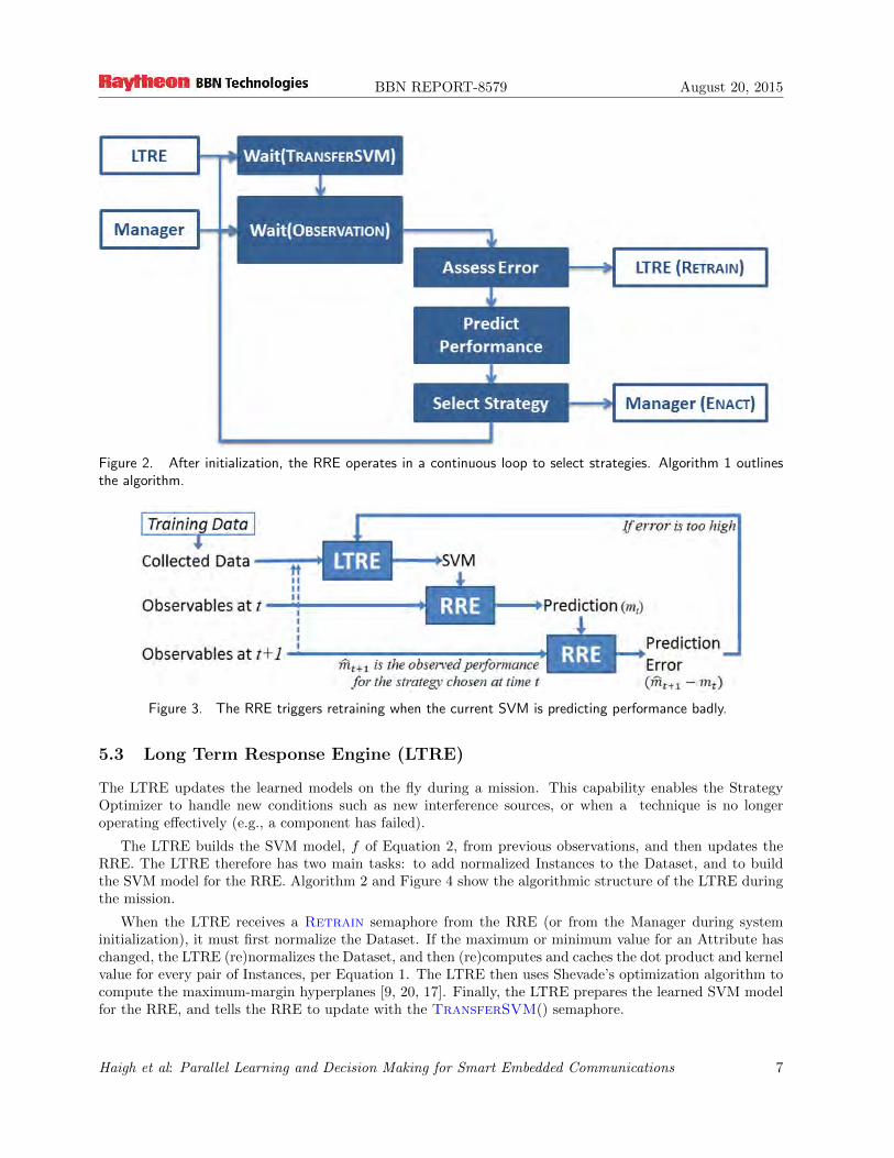
Algorithm 1 and Figure 2 show the operation of the RRE. Once the RRE receives the initial SVM modelfrom the LTRE with the TransferSVM() semaphore, it operates on each new observation in a continuousloop, waiting for the Observation() semaphore.

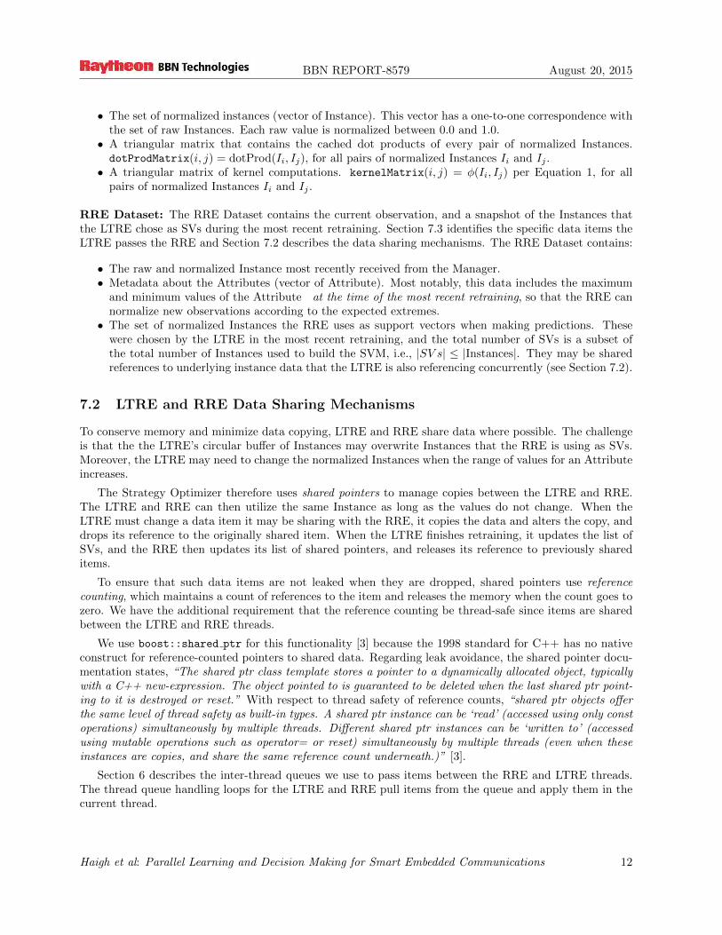
It first asesses the quality of the current SVM model: if the predicted value of the metric at time t− 1,mt−1, is outside of a certain tolerance of the observed value at time t, mt, then the model needs to beretrained (Figure 3):

if |mt−1 − mt| > τ, thentrigger retraining using Retrain semaphore

The RRE then predicts the performance of each of the available strategies in the current environment.It uses the previously-learned SVM model, f = (o, s) of Equation 2, to make this prediction:

for each candidate strategy s in Sms = SVM(o, s)

Finally, the RRE selects the single strategy with the best expected performance, and then sends Enact()semaphore to tell the Manager.



Figure 2. After initialization, the RRE operates in a continuous loop to select strategies. Algorithm 1 outlinesthe algorithm.

Figure 3. The RRE triggers retraining when the current SVM is predicting performance badly.

5.3 Long Term Response Engine (LTRE)

The LTRE updates the learned models on the fly during a mission. This capability enables the StrategyOptimizer to handle new conditions such as new interference sources, or when a technique is no longeroperating effectively (e.g., a component has failed).

The LTRE builds the SVM model, f of Equation 2, from previous observations, and then updates theRRE. The LTRE therefore has two main tasks: to add normalized Instances to the Dataset, and to buildthe SVM model for the RRE. Algorithm 2 and Figure 4 show the algorithmic structure of the LTRE duringthe mission.

When the LTRE receives a Retrain semaphore from the RRE (or from the Manager during systeminitialization), it must first normalize the Dataset. If the maximum or minimum value for an Attribute haschanged, the LTRE (re)normalizes the Dataset, and then (re)computes and caches the dot product and kernelvalue for every pair of Instances, per Equation 1. The LTRE then uses Shevade’s optimization algorithm tocompute the maximum-margin hyperplanes [9, 20, 17]. Finally, the LTRE prepares the learned SVM modelfor the RRE, and tells the RRE to update with the TransferSVM() semaphore.



ALGORITHM 2: The LTRE updates the learned models during a mission so that the Strategy Optimizer can handle

new interference conditions or recognize when techniques are no longer operating effectively. Figure 4 illustrates the

functional flow.Input: It: Instance from RRE at time t, containing vector < ot, ct,mt > of observables, controllables, and metricOutput: SVM: Support Machine for the RRE, per Equation 2, which includes the offset b, the Support Vectors

(SVs), and their corresponding α valuesSemaphore: Observation(It) from Manager during missionSemaphore: Retrain from RRE during mission, from Manager during system initializationSemaphore: Terminate from Manager at mission end

repeat in parallelwait until Observation(It) semaphore // Process all pending Instances before Retrain

if |Dataset| >MAXINSTANCES then // Circular BufferRemove oldest I from Dataset

endAppend It to Datasetforeach observable oi ∈ ot do

if oi > Attribute[i].max or oi < Attribute[i].min then // Flag for renormalizationSet Renormalization flag for Attribute[i] to true

end

endforeach Instance I ∈ Dataset do // Cache items needed for Retraining

Compute dotProd(It, I)Compute φ(It, I) using Equation 1

end

endwait until Retrain semaphore

if ∃ Attribute with Renormalization flag set to true, thenRenormalize Dataset // Renormalizeforeach pair of Instances I1, I2 ∈ Dataset do // Recompute Cached items

Compute dotProd(I1, I2)Compute φ(I1, I2) using Equation 1

end

endCompute SVs using SMO [20] // RetrainSVM ← // Copy SVs for RRE

foreach sv ∈ SVs doSave offset b for RRE

Save αδsv = αsv − α∗sv for RRE

Make shared pointer to sv for RRE

end

Trigger semaphore TransferSVM(SVM) to RRE

end

until semaphore Terminate

When the LTRE receives a new Instance with the Observation() semaphore, it first checks whether thebounds have changed, and if so, flags the Attribute for renormalization. It then adds the Instance to theDataset, and computes its dot products and kernel values to all other Instances. To live within the memorybounds on the embedded platform, the LTRE uses a circular buffer of Instances; when the bound is reached,the LTRE overwrites the oldest Instance. Note that the LTRE will add all pending Instances before startinga new retraining.

Note that the original implementation of Weka renormalizes the data, and then calls SMO. SMO computes



Figure 4. The LTRE manages the Dataset and rebuilds the learned models. Algorithm 2 outlines the algorithm.

all the dot products and φ kernel values internally. Because we may not need to renormalize our data atevery retraining, we move this computation outside SMO.

6 Threading Model

There are three key threads in the Strategy Optimizer, corresponding to each of the components of Section 5.The Manager is the highest priority thread, as it must respond to incoming data immediately. It buffersthe incoming data and queues messages for the RRE. The RRE is the second highest priority, and makesstrategy decisions for current conditions. The LTRE is a lower priority thread, where the Strategy Optimizerlearns models of how the strategies perform.

Figure 5 shows the sequence diagram of the pre-mission initialization, and the in-mission runtime loop.On startup, the LTRE thread makes its first SVM and notifies the RRE; the mission can start after this firstSVM is ready. At runtime, the RRE makes an Instance for every observation that it receives. It then checksto see if the observed performance matches the predicted performance; if there was sufficient prediction error,the RRE triggers retraining in the LTRE. The RRE then predicts the performance for each available strategyin the current communications conditions, and selects the strategy with the highest expected performancefor the next round.

We use a Mailbox to pass objects (actions or data) between threads. The mailbox is implemented as amax-depth queue.

• The Manager uses a depth-one queue to send data to the RRE, so that the RRE operates on only themost recent data.



Figure 5. The LTRE builds its first SVM before the mission starts. During the mission the RRE processes eachobservation, and triggers retraining when necessary.

• The LTRE uses a depth-one queue to send updated SVM models to the RRE.• The RRE uses a depth-d queue to send data to the LTRE because retraining a single SVM can span

a temporal duration where the RRE receives many messages. Figure 6 illustrates a potential sequenceof retraining interactions between the RRE and the LTRE. When the LTRE completes a retraining, itadds any pending Instances in the queue to the Dataset, then (if necessary) starts a new retraining.

7 Data Management

During initialization, the LTRE builds an SVM based on its initial training data; the RRE waits until thisfirst SVM is ready. Then during the mission, the RRE processes every new observation while the LTREwaits for a retraining signal. If the RRE detects sufficient prediction error, then it triggers retraining; atthis point the RRE and the LTRE are operating in parallel.

As it retrains, the LTRE must ensure that it does not alter any data supporting the RRE’s existing SVMsince the RRE thread is still using it to predict. While maintaining thread safety of this data, we must alsominimize memory usage and data copy overhead.

7.1 Data Elements

The LTRE and RRE both use Instances to represent the observations of the communications environment. ADataset is the wrapper class for all of the Instances. It maintains a set of Attributes, each of which containsmeta-information about an observable or controllable, such as its maximum & minimum & mean values. ADataset also contains derived calculations such as the pairwise dot products and kernel computations.



Figure 6. The LTRE operates on the most recent retraining request,and adds all pending observations to the Dataset.

7.1.1 Instance

The RRE uses the current Instance to predict performance of the available strategies. The LTRE uses the setof Instances to train the SVM, and selects a subset of these Instances to become Support Vectors. The keyitem in an Instance is a vector of values that describe each attribute from the observations, the observableso, the controllables c, and the metric m.

The RRE creates two independent copies of each incoming Instance: one for the RRE to use to predictmetrics, and one for the LTRE to add to the Dataset for subsequent LTRE retraining.

The LTRE adds each Instance to its Dataset, and then when the RRE requests a retrain, the LTREtrains on the set of Instances in memory. When the LTRE finishes processing the training data, it makesreferences to the set of Instances that it selected as support vectors, and passes the references to the RRE(Section 7.3).

7.1.2 Dataset

The Dataset contains SVM-supporting data and data-related functionality. The LTRE and RRE eachmaintain separate datasets, though both may be referencing the same underlying Instance data, using sharedpointers (Section 7.2). Both types of Dataset maintain Instance metadata such as a mapping of Attributecolumns to Instance indices and Attribute value min/max/mean.

LTRE Dataset: The LTRE Dataset contains all the data required to build SVMs:

• Metadata about the Attributes (vector of Attribute).• The set of raw training Instances (vector of Instance). This vector includes Instances that have been

processed by the RRE but the LTRE has yet to incorporate into a new model by retraining. Thisvector is managed as a circular fixed-length buffer; when the vector is full, the LTRE overwrites theoldest Instance.



• The set of normalized instances (vector of Instance). This vector has a one-to-one correspondence withthe set of raw Instances. Each raw value is normalized between 0.0 and 1.0.• A triangular matrix that contains the cached dot products of every pair of normalized Instances.dotProdMatrix(i, j) = dotProd(Ii, Ij), for all pairs of normalized Instances Ii and Ij .• A triangular matrix of kernel computations. kernelMatrix(i, j) = φ(Ii, Ij) per Equation 1, for all

pairs of normalized Instances Ii and Ij .

RRE Dataset: The RRE Dataset contains the current observation, and a snapshot of the Instances thatthe LTRE chose as SVs during the most recent retraining. Section 7.3 identifies the specific data items theLTRE passes the RRE and Section 7.2 describes the data sharing mechanisms. The RRE Dataset contains:

• The raw and normalized Instance most recently received from the Manager.• Metadata about the Attributes (vector of Attribute). Most notably, this data includes the maximum

and minimum values of the Attribute at the time of the most recent retraining, so that the RRE cannormalize new observations according to the expected extremes.• The set of normalized Instances the RRE uses as support vectors when making predictions. These

were chosen by the LTRE in the most recent retraining, and the total number of SVs is a subset ofthe total number of Instances used to build the SVM, i.e., |SV s| ≤ |Instances|. They may be sharedreferences to underlying instance data that the LTRE is also referencing concurrently (see Section 7.2).

7.2 LTRE and RRE Data Sharing Mechanisms

To conserve memory and minimize data copying, LTRE and RRE share data where possible. The challengeis that the the LTRE’s circular buffer of Instances may overwrite Instances that the RRE is using as SVs.Moreover, the LTRE may need to change the normalized Instances when the range of values for an Attributeincreases.

The Strategy Optimizer therefore uses shared pointers to manage copies between the LTRE and RRE.The LTRE and RRE can then utilize the same Instance as long as the values do not change. When theLTRE must change a data item it may be sharing with the RRE, it copies the data and alters the copy, anddrops its reference to the originally shared item. When the LTRE finishes retraining, it updates the list ofSVs, and the RRE then updates its list of shared pointers, and releases its reference to previously shareditems.

To ensure that such data items are not leaked when they are dropped, shared pointers use referencecounting, which maintains a count of references to the item and releases the memory when the count goes tozero. We have the additional requirement that the reference counting be thread-safe since items are sharedbetween the LTRE and RRE threads.

We use boost::shared ptr for this functionality [3] because the 1998 standard for C++ has no nativeconstruct for reference-counted pointers to shared data. Regarding leak avoidance, the shared pointer docu-mentation states, “The shared ptr class template stores a pointer to a dynamically allocated object, typicallywith a C++ new-expression. The object pointed to is guaranteed to be deleted when the last shared ptr point-ing to it is destroyed or reset.” With respect to thread safety of reference counts, “shared ptr objects offerthe same level of thread safety as built-in types. A shared ptr instance can be ‘read’ (accessed using only constoperations) simultaneously by multiple threads. Different shared ptr instances can be ‘written to’ (accessedusing mutable operations such as operator= or reset) simultaneously by multiple threads (even when theseinstances are copies, and share the same reference count underneath.)” [3].

Section 6 describes the inter-thread queues we use to pass items between the RRE and LTRE threads.The thread queue handling loops for the LTRE and RRE pull items from the queue and apply them in thecurrent thread.



7.3 Shared Data Items

Section 7.1 describes the data elements that the LTRE and RRE maintain. Section 7.2 outlines the mecha-nisms used by the LTRE and RRE to share data. This section identifies the data items that we pass betweenthe LTRE and RRE during operation.

When the LTRE builds an SVM initially or on retrain, it must make a copy of the learned model for theRRE. Algorithm 2 shows the pseudocode for this step. It copies a set of model parameters to the RRE touse for predicting performance metric values:

• A timestamp indicating when the SVM was built (64-bit integer). The RRE uses the timestamp aspart of error analysis to match predictions to the SVM incarnation in use, and to make sure that itdoesn’t request a retrain on an unused SVM.• The list of Support Vectors (vector of shared pointer to Instance). This is the list of normalized

Instances selected to be SVs, and then sorted for pipelining.• Alpha delta values (vector of float). Set of (αδi = αi − α∗i ), sorted for pipelining, matching one-to-one

with the SVs.• Support Vector self-dot-products (vector of float). This vector is the diagonal of the Instance dot

product matrix of each SV to itself• Attribute metadata (vector of Attribute). See Section 7.1.2.• Coefficients used by the SVM normalization filter for doing its linear transformation. (3 x int) b, x0

and x1.

7.4 System Operation

The LTRE, upon receiving a new Instance from the Manager, adds the Instance to its Dataset. When theLTRE next retrains, these new Instances are considered as candidate SVs. To place an upper bound on itsmemory use, the LTRE constrains its instance set to maximum size fixed at compile time. When a newInstance would exceed this maximum, the LTRE deletes the oldest Instance reference in its Dataset, andthen adds the new one. The shared pointer implementation (Section 7.2) reduces the reference count to theInstance, and releases the memory if and only if the RRE is not using it. (The deleted Instance referencemay be pointing to one of the SVs chosen in the previous retrain and currently in use by the RRE.)

Figure 7 shows how the LTRE and RRE Instance sets can diverge over time due to circular buffering,but then re-align after the LTRE retrains. When the RRE receives the results of the retrain, it releases itsreferences to the old Instances, which releases the underlying Instance data because the reference count hasreached zero.

Figure 8 illustrates another cause of divergence between the LTRE and RRE Instance sets: renormaliza-tion. In this case, the LTRE releases references to its entire normalized Instance set (while the RRE retainsits references) and creates a new set of normalized Instances. The LTRE and RRE Instance sets re-alignafter the LTRE retrain completes, with the RRE releasing the data associated with the old Instances.

8 Results

We performed our experiments using a suite of 18 different environmental conditions that varied the commu-nications traffic requirements, mobility patterns and interference. There are 160 strategies, generated fromlegal combinations of 9 control parameters. We present the following results:

• Section 8.1: Compare dynamic Strategy Optimizer to a static system with one prechosen strategy.• Section 8.2: Compare incremental learning to a system that starts with learned models, but then

doesn’t change.



(1) During Initial Training:LTRE builds a model using allInstances.

(4) After Retraining: RREcopies pointers to new setof SVs, and discards unusedpointers.

(2) After Initial Training: RRE copiespointers to Instances chosen as SVs.

(5) During retraining: LTRE adds newInstances and overwrites the circularbuffer and discards unused Instances.RRE is unchanged.

(3) During Retraining: LTRE addsmore instances. RRE is unchanged.

(6) After Retraining: RRE copiespointers to new set of SVs, anddiscards unused pointers.

Figure 7. At the end of each retraining (states 2, 4 and 6), RRE and LTRE operate on the same set of Instances.During retraining, RRE may be using a different set of pointers, because the LTRE’s circular buffer has overwrittenprevious Instances (state 5), or because the LTRE has renormalized Instances (per Figure 8).

(1) After Initial Training:RRE and LTRE use thesame set of underlyingnormalized Instances.

(2)After Renormalization, during Retraining: RRE usesthe original normalized Instances. LTRE creates anew set using the new Attribute min/max.

(3)After Retraining: RREand LTRE use the sameset of underlying normal-ized Instances.

Figure 8. Renormalizing causes RRE and LTRE to get out of synch during retraining. After retraining, theyresynchronize, and discard any unused Instances.

• Section 8.3: A detailed incremental learning example.• Section 8.4: n-choose-k incremental learning, from no a priori data to full a priori data.• Section 8.5: Parallel RRE decision making and LTRE incremental learning.

8.1 Comparison to a Static, Manually-Configured System

Compare system with one fixed strategy to system that switchs as conditions change.

The Strategy Optimizer performs significantly better when it can choose what CPs to use for each condition.Figure 9 shows two of the many examples in which our dynamic Strategy Optimizer performs better than astatic system.



Figure 9. By adaptively choosing and combining different strategies as the environ-ment changes, the Strategy Optimizer performs better than a system that only hasone available. Top graph shows observed performance. Bottom graph shows strategychosen by the dynamic Strategy Optimizer, as a combination of CPs. X axis is time.

8.2 Comparison to a Learning-Configured System with no Incremental Retrain-ing

Both systems start with a learned model, but one system doesn’t allow on-the-fly retrains.

Incremental Learning is Strategy Optimizer’s critical ability to start from limited knowledge and incremen-tally improve performance during a simulation. Figure 10 shows a trace where the Strategy Optimizer wasconfigured to do no retraining. The simulation encountered four similar RF conditions, but was not trainedon any of these. The Strategy Optimizer achieves an average performance of 274.9 across all 40 timestamps,achieving optimal performance from time 21 to 31. On average, however, it only achieves 31% of what itcould have achieved for the sequence. In Figure 11, the Strategy Optimizer retrains when prediction erroris 100% (either the prediction is double the observation, or the observation is double the prediction). Onlythree retrainings are required to obtain an average performance of 820.8. Compared to optimal performance,the Strategy Optimizer achieves 94% of what it could have achieved for the sequence.

8.3 Detailed Trace with Incremental Learning

Partial training; RRE detects error, LTRE fully retrains, then RRE finishes.

Figure 12 and Figure 13 show a set of detailed results from an incremental learning trace involving 18conditions. Condition #4 and all other similar conditions were not present in the training data. TheStrategy Optimizer was configured to retrain the SVM models when prediction error was 50%. In the largerectangle, Figure 12 highlights time units 30-40, where the Strategy Optimizer encounters condition #4 forthe first time. Figure 13 shows the details of throughput predictions for five of the 160 strategies. At timeunit 30, the Strategy Optimizer chooses the strategy that uses CP6 and CP3; unfortunately, performance



Figure 10. Performance averages 274.9 when theStrategy Optimizer is not allowed to retrain its mod-els when it encounters new conditions. This is 31%of optimal.

Figure 11. Performance averages 820.8 when theStrategy Optimizer is allowed to retrain in-mission;only three retrainings occur. This is 94% of optimal.

Top graph is observed performance, middle graph is chosen strategy, bottom graph is binary indicator ofretraining.

is zero, and prediction error is very high. The Strategy Optimizer retrains its models, but at time unit31, it makes a similar prediction. The training data very strongly indicates that CP6+3 will perform well:there are no examples in the training data in which it performs poorly. Essentially, this one observation ofzero performance is treated as an outlier. Two more examples of zero performance for CP6+3 cause theStrategy Optimizer to switch strategies at time unit 33, and choose CP6+5. This time, only one examplecauses the Strategy Optimizer to switch. At time unit 34, it chooses CP5, and gets significantly improvedperformance. If the mission configuration set a minimum performance, the Strategy Optimizer could stopswitching strategies at this point. By time unit 38, the Strategy Optimizer has found the optimal strategy,which achieves a Throughput of 750.0.

In the smaller rectangles, Figure 12 shows the long-term effect of the experience with condition #4.For all eight of the other similar conditions, the Strategy Optimizer gets excellent performance. Overallperformance averages 93.1% of optimal across the simulation. The Strategy Optimizer is able to generalizethe characteristics from condition #4 to the other cases. Note that it does not always choose the samestrategy, and that the optimal performance is not always 750.0.

8.4 Aggregate Incremental Learning

All combinations of partial learning traces.

Figure 14 shows the results of an n-choose-k ablation study for incremental learning. We tested the StrategyOptimizer against n = 9 environmental conditions. In each experiment, the initial training data containswith a different subset k of these conditions, corresponding to the x axis. Each point therefore shows theperformance of an experiment in which the Strategy Optimizer performs incremental learning as needed.1

The chart shows that performance compared to optimal is 99.3% when the Strategy Optimizer trains onall available training data, and that performance gracefully degrades when the Strategy Optimizer is trainedwith fewer conditions. When the Strategy Optimizer trains on nothing2, then performance compared tooptimal is 68.4%.

1Section 8.3 would correspond to one point on Figure 14.2Training on nothing means that there are only two legal instances, loosely corresponding to when no detected energy yields

no expected performance: (NaN, NaN, . . . , NaN → NaN) and (0, 0, . . . , 0 → 0).



Figure 12. The Strategy Optimizer generalizes from its experience with condition #4 (large overlay rectangle)to perform well on other similar new emitters (smaller rectangles). Top graph shows predicted values for all 160strategies; note that optimal performance varies with condition. Middle graph shows observed value at time t.Lower graph shows chosen strategy, as a combination of CPs. X-axis is time.

8.5 Timing Performance and Threading

Parallel RRE decision making and LTRE incremental learning.

Table 1 shows the timing results for one communications scenario on our Linux server and our two em-bedded platforms. The RRE compute time is linear in the number of strategies considered, while LTRE isapproximately linear in the number of Instances used for training. In addition, when the underlying data isrelatively redundant, it is faster to train the model, and fewer Instances are selected as SVs for the RRE.

Linux ARMv7 PPC440RRE 11ms 303ms 8,201msLTRE retrain only 11ms 334ms 8,854msLTRE renorm+retrain 64ms 1,292ms 17,385ms

Table 1. Renormalizing the dataset requires floating-point divides, and takes a significantamount of time compared to the RRE and the LTRE when no renormalization is necessary.

Figure 15 and Figure 16 show the impact of sharing the CPU between the two threads. As the LTREis given more CPU, the LTRE latency drops while the RRE latency increases. Table 2 shows the raw dataunderlying this plot. The shape of the curve is the same for PPC440. Note that the PPC440 platform usesa Real-Time Operating System, and thus we can directly control the CPU usage.



Figure 13. Only a small number of training exemplars causes the Strategy Optimizer to choosedifferent strategies. Each “CP” column shows the predicted performance values for that strategy.A box indicates the strategy chosen by the Strategy Optimizer at time t. The “Observed” columnshows the actual value from test harness at time t + 1, and used by the Strategy Optimizer todecide whether to retrain the model.

ARMv7%CPU for LTRE RRE latency (ms) # RREs per LTRE LTRE latency (ms)

0% 303 N/A N/A1% 306 110 36,7405% 319 21 7,014

10% 337 10 3,34020% 379 5 1,67025% 404 4 1,33650% 606 2 668

PPC440%CPU for LTRE RRE latency (ms) # RREs per LTRE LTRE latency (ms)

0% 8,200 N/A N/A1% 8,283 107 946,2425% 8,632 21 181,602

10% 9,111 10 86,02220% 10,250 5 38,23225% 10,933 4 28,67450% 16,400 2 9,558

Table 2. When the LTRE has 1% of the CPU, the RRE makes approximately 110 decisions while theLTRE is retraining a new model. As the LTRE is given more CPU, LTRE latency drops while RRE latencyincreases.



Figure 14. An n-choose-k ablation trial shows that the performance gracefully degrades as theStrategy Optimizer’s a priori training data contains fewer conditions. Each point corresponds to theperformance of one experiment; the x-axis is k showing how many conditions were present in thetraining dataset, and the y-axis is the Performance-against-optimal value. In each column of points,we annotate that there are (X) experiments for 9-choose-k.

Figure 15. On ARMv7, RRE takes 303ms to computewhen has full use of the processor. As the LTRE usesmore CPU, the RRE has more latency to produce adecision. Table 2 shows the underlying data.

Figure 16. On ARMv7, LTRE takes 334ms to com-pute when it does not need to renormalize values andit has full use of the processor. As the LTRE uses lessCPU, the LTRE has more latency to retrain the model.



9 Conclusion

This paper described our effort to place Machine Learning on an embedded communications system. OurStrategy Optimizer has a rapid decision-making loop that selects a configuration in real-time to optimizeperformance of the network as conditions change. The Strategy Optimizer also has a slower learning loopthat updates the prediction models as the system encounters novel conditions.

In this paper, we focused on the threading model and data interchange mechanisms required for the twoloops to operate in parallel. We presented results showing the accuracy of the decisions, and showing howthe thread parallelism affects the latency of decisions.

Our multi-threaded structure, and the semantically-agnostic nature of the learner (i.e., it uses no labels),ensure that our approach is relevant for any embedded system that wishes to incorporate Machine Learningto make rapid decisions in a complex environment.

Acknowledgments

This work represents collaboration with BAE Systems (Merrimack, NH). We thank with gratitude John Tran-quilli (BAE), Amber Dolan (BAE), Bruce Fette (formerly DARPA), and Vincent Sabio (formerly DARPA).

The views, opinions, and/or findings contained in this article/presentation are those of the author(s)/presenter(s) and should not be interpreted as representing the official views or policies of the Department ofDefense or the U.S. Government.

Distribution Statement “A” (Approved for Public Release, Distribution Unlimited).

References

[1] Applied Micro Circuits Corporation. PPC440 (PPC440G5) Processor User’s Manual, 1.0 edition, Au-gust 2011. http://www.amcc.com.

[2] Haifeng Chen, Guofei Jiang, Hui Zhang, and Kenji Yoshihira. Boosting the performance of computingsystems through adaptive configuration tuning. In Proc. ACM Symposium on Applied Computing (SAC),pages 1045–1049. (New York, NY: ACM Press), 2009.

[3] Greg Colvin, Beman Dawes, Darin Adler, and Peter Dimov. Boost c++ libraries: shared ptr classtemplate, 1999. http://www.boost.org/doc/libs/1 56 0/libs/smart ptr/shared ptr.htm.

[4] Fangwen Fu and Mihaela van der Schaar. Decomposition principles and online learning in cross-layeroptimization for delay-sensitive applications. IEEE Transactions on Signal Processing, 58(3):1401–1415,2010. http://ieeexplore.ieee.org/stamp/stamp.jsp?arnumber=5290102.

[5] Karen Zita Haigh. AI technologies for tactical edge networks. In MobiHoc 2011 Workshop on TacticalMobile Ad Hoc Networking, Paris, France, 2011. (New York, NY: ACM Press). Keynote address.http://www.cs.cmu.edu/∼khaigh/papers/Haigh-MobiHoc2011.pdf.

[6] Karen Zita Haigh, Allan M. Mackay, Michael R. Cook, and Li L. Lin. Machine learning for embeddedsystems: A case study. Technical Report BBN REPORT 8571, BBN Technologies, Cambridge, MA,March 2015. http://www.cs.cmu.edu/∼khaigh/papers/2015-HaighTechReport-Embedded.pdf.

[7] Karen Zita Haigh, Olu Olofinboba, and Choon Yik Tang. Designing an implementable user-oriented objective function for MANETs. In IEEE International Conference On Networking,Sensing and Control, pages 693–698, London, U.K., April 2007. (New York, NY: IEEE Press).http://www.cs.cmu.edu/∼khaigh/papers/Haigh07-ICNSC.pdf.


http://www.amcc.com

http://www.boost.org/doc/libs/1_56_0/libs/smart_ptr/shared_ptr.htm

http://ieeexplore.ieee.org/stamp/stamp.jsp?arnumber=5290102

http://www.cs.cmu.edu/~khaigh/papers/Haigh-MobiHoc2011.pdf

http://www.cs.cmu.edu/~khaigh/papers/2015-HaighTechReport-Embedded.pdf

http://www.cs.cmu.edu/~khaigh/papers/Haigh07-ICNSC.pdf


[8] Karen Zita Haigh, Srivatsan Varadarajan, and Choon Yik Tang. Automatic learning-based MANET cross-layer parameter configuration. In Workshop on Wireless Ad hoc andSensor Networks (WWASN2006), Lisbon, Portugal, 2006. (New York, NY: ACM Press).http://www.cs.cmu.edu/∼khaigh/papers/haigh06a-configuration.pdf.

[9] Mark Hall, Eibe Frank, Geoffrey Holmes, Bernhard Pfahringer, Peter Reutemann, and Ian H.Witten. The WEKA data mining software: An update. SIGKDD Explorations, 11(1), 2009.http://www.cs.waikato.ac.nz/∼eibe/pubs/weka update.pdf.

[10] Ovidiu Ivanciuc. Support vector machine software, 2005. http://www. support-vector-machines.org/SVM soft.html.

[11] V. Kawadia and P. R. Kumar. A cautionary perspective on cross-layer design. IEEE Wireless Commu-nication, 12(1):3–11, 2005. http://ieeexplore.ieee.org/xpls/abs all.jsp?arnumber=1404568.

[12] Xiaojun Lin, Ness B. Shroff, and R. Srikant. A tutorial on cross-layer optimization in wire-less networks. IEEE Journal on Selected Areas in Communications, 24(8):1452–1463, 2006.http://www.ifp.illinois.edu/ srikant/Papers/linshrsri06.pdf.

[13] Joseph Mitola III. Cognitive Radio: An Integrated Agent Architecture for Software Defined Radio. PhDthesis, Kista, Sweden, 2000. http://www.diva-portal.org/smash/get/diva2:8730/FULLTEXT01.pdf.

[14] D. Montana, T. Hussain, and T. Saxena. Adaptive reconfiguration of data networks using genetic algo-rithms. In Proc. Genetic and Evolutionary Computation Conference (GECCO), pages 1141–1159. (NewYork, NY: ACM Press), 2002. http://citeseerx.ist.psu.edu/viewdoc/summary?doi=10.1.1.152.8686.

[15] T. R. Newman, R. Rajbanshi, A. M. Wyglinski, J. B. Evans, and G. J. Min-den. Population adaptation for genetic algorithm-based cognitive radios. In Proc.of ICST Conference on Cognitive Radio Oriented Wireless Networks and Communi-cations (CROWNCOM), pages 279–284. (New York, NY: IEEE Press), May 2007.http://www.ittc.ku.edu/∼newman/publications/Conferences/crowncom2007 newman rajbanshi wyglinski evans minden.pdf.

[16] Timothy Newman, Joseph Evans, and Alexander Wyglinski. Reconfiguration, adaptation and opti-mization. In Alexander M. Wyglinski, Maziar Nekovee, and Thomas Hou, editors, Cognitive RadioCommunications and Networks: Principles and Practice. (New York, NY: Elsevier/North Holland),2009.

[17] John C Platt. Fast training of Support Vector Machines using Sequential Minimal Optimization. InB. Schoelkopf, C. Burges, and A. Smola, editors, Advances in Kernel Methods - Support Vector Learn-ing. (Cambridge, MA: MIT Press), 1998. http://research.microsoft.com/en-us/um/people/jplatt/smo-book.pdf.

[18] C. J. Rieser. Biologically Inspired Cognitive Radio Engine Model Utilizing Distributed Genetic Algo-rithms for Secure and Robust Wireless Communications and Networking. PhD thesis, Virginia Tech,Blacksburg, VA, 2004. http://scholar.lib.vt.edu/theses/available/etd-10142004-023653/.

[19] Thomas W. Rondeau. Application of Artificial Intelligence to Wireless Communications. PhD thesis,Department of Electrical Engineering, Virginia Polytechnic Institute, Blacksburg, VA, September 2007.http://scholar.lib.vt.edu/theses/available/etd-10052007-081332/.

[20] S. K. Shevade, S. S. Keerthi, C. Bhattacharyya, and K. R. K. Murthy. Improvements to thesmo algorithm for svm regression. IEEE Transactions on Neural Networks, 11(5), Sept 2000.http://www.keerthis.com/smoreg ieee shevade 00.pdf.


http://www.cs.cmu.edu/~khaigh/papers/haigh06a-configuration.pdf

http://www.cs.waikato.ac.nz/~eibe/pubs/weka_update.pdf

http://www.support-vector-machines.org/SVM_soft.html

http://www.support-vector-machines.org/SVM_soft.html

http://ieeexplore.ieee.org/xpls/abs_all.jsp?arnumber=1404568

http://www.ifp.illinois.edu/~srikant/Papers/linshrsri06.pdf

http://www.diva-portal.org/smash/get/diva2:8730/FULLTEXT01.pdf

http://citeseerx.ist.psu.edu/viewdoc/summary?doi=10.1.1.152.8686

http://www.ittc.ku.edu/~newman/publications/Conferences/crowncom2007_newman_rajbanshi_wyglinski_evans_minden.pdf

http://www.ittc.ku.edu/~newman/publications/Conferences/crowncom2007_newman_rajbanshi_wyglinski_evans_minden.pdf

http://research.microsoft.com/en-us/um/people/jplatt/smo-book.pdf

http://research.microsoft.com/en-us/um/people/jplatt/smo-book.pdf

http://scholar.lib.vt.edu/theses/available/etd-10142004-023653/

http://scholar.lib.vt.edu/theses/available/etd-10052007-081332/

http://www.keerthis.com/smoreg_ieee_shevade_00.pdf


[21] Ryan W. Thomas, Daniel H. Friend, Luiz A. DaSilva, and Allen B. MacKenzie. Cognitive networks:Adaptation and learning to achieve end-to-end performance objectives. IEEE Communications Maga-zine, pages 51–57, December 2006. http://ieeexplore.ieee.org/xpl/articleDetails.jsp?arnumber=4050101.

[22] Gregory D. Troxel, Armando Caro, Isidro Castineyra, Nick Goffee, Karen Zita Haigh, Talib Hussain,Vikas Kawadia, Paul G. Rubel, and David Wiggins. Cognitive adaptation for teams in ADROIT. InIEEE Global Communications Conference, pages 4868–4872, Washington, DC, November 2007. (NewYork, NY: IEEE Press). Invited. http://www.cs.cmu.edu/∼khaigh/ papers/troxel07-globecom.pdf.

[23] B. Ustun, W. J. Melssen, and L. M. C. Buydens. Facilitating the applicationof Support Vector Regression by using a universal Pearson VII function based ker-nel. Chemometrics and Intelligent Laboratory Systems, 81(1):29–40, March 2006.http://www.sciencedirect.com/science/article/pii/S0169743905001474.

[24] Vladimir N. Vapnik. The Nature of Statistical Learning Theory. (New York, NY: Springer), 1995.

[25] Wikipedia. Support vector machine, 2014. http://en.wikipedia.org/wiki/ Support vector machine,downloaded October 2014.


http://ieeexplore.ieee.org/xpl/articleDetails.jsp?arnumber=4050101

http://www.cs.cmu.edu/~khaigh/papers/troxel07-globecom.pdf

http://www.sciencedirect.com/science/article/pii/S0169743905001474

http://en.wikipedia.org/wiki/Support_vector_machine

Date post:	30-Jan-2022
Category:	Documents
Upload:	others
View:	1 times
Download:	0 times

Parallel Learning and Decision Making for a Smart Embedded ...

Documents