Parallel Linear Programming in Fixed Dimension Almost Surely in Constant Time

NOGA ALON AND NIMROD MEGIDDO

IBM Abnadeiz Research Cetlter; Sail Jose. Culdomia and Tel-Ark Unir'ersity. Tel-Ariv, Israel

Abstract. For any futed dimension d, the linear programming problem with IZ inequality con- straints can be solved on a probabilistic CRCW PRAM with O ( n ) processors almost surely in constant time. The algorithm always finds the correct solution. With nd/log% processors, the probability that the algorithm wlll not finish withm O(d'1og2d) time tends to zero exponentially wlth 11.

Categories and Subject Dcscriptors: G.l.O [Numerical Analysis]: General-parallel algontlznts: G.1.6 [Numerical Analysis]: Optimization-hnear programlhrzg; G.3 [Probability and Statistics]: prohablhstlc algontlzms (~~ tc lud~ng Monte CarloI

General Terms: Algorithms, Theory

Additional Key Words and Phrases: Computational geometry, linear programming, multidimen- sional search. parallel computation, probabilistic computation

The linear programming problem in fixed dimension is to maximize a linear function of a fixed number, d, of variables, subject to rz linear inequality c onstraints, where n is not fixed. Megiddo [I9831 showed that, for any d, this problem can be solved in 0 ( n ) time. Clarkson [I9861 and Dyer [I9861 improved the constant of proportionality. Clarkson [I9881 later developed linear-time probabilistic algorithms with even better complexity. The problem in fixed dimension is interesting from the point of view of parallel computation, since the general linear programming problem is known to be P-complete. The algorithm of Megiddo [I9841 can be parallelized efficiently, but the exact parallel complexity of the problem in fixed dimension is still not known.' Here, we develop a very efficient probabilistic, based on Clarkson's [I9881 scheme.

1 . . Aj ta~ and Megiddo recently devclopcd deterministic algorithms that run on a linear number of processors in poly-loglog time.

Thls research was supported in part by the Officc of Naval Research (ONR) under contract N00014-87-C-0820.

Authors' present addresses. N. Alon, School of Mathematical Sciences, Tcl Avlv University. Tel Aviv, Israel. Email: noga@&~math.tau.ac.il: N. Meglddo. IBM Almaden Research Center, 650 Harry Road. K53/S07. San Jose. CA 95120-6099. Emall: megiddo@~almaden.ibm.com. Permmion to copy without fee all or part of thls material is granted provlded that the copies are not made or distributed for direct commercial advantage, the ACM copyright notice and the title of the publication and ~ t s date appear, and notice is glvcn that copying is by permission of the Association for Computing Machinery. To copy othenvisc, or to republish, requires a fee and/or specific permission. GJ 1993 ACM 0003-541 1/94/0100-0322 $03.50

J o u ~ n d l of thr Awruat lon tor Cornputmg Mdchmcry, Vol 41, No 2, March 1YL14. pp 123-434

Linear Programming in Constant Time 423

In this paper, when we say that a sequence of events { E , , } ~ , , occurs almost surely, we mean that there exists an E > 0 such that prob( Ell ) r 1 - exp( -a'). A consequence of this estimate is that, with probability 1, only a finite number of the events do not occur. The main result of this paper generalizes a known fact [Reischuk, 1981; Megiddo, 19821 that the maximum of FZ items can be computed almost surely in constant time.

As mentioned above, the basic idea of the underlying sequential algorithm is due to Clarkson [1988]. His beautiful iterative sequential algorithm uses an idea of Welzl [19881. As in Clarkson's algorithm, we also sample constraints repeatedly with variable probabilities. Several additional ideas and some modi- fications were, however, required in order to achieve the result of this paper. Our probabilistic analysis is also different, and focuses on probabilities of failure to meet time bounds, rather than on expected running times. In particular, a suitable sequential implementation of our algorithm can be shown to terminate almost surely within the best known asymptotic bounds on the expected time.

In Section 2, we present a special form of the output required from a linear programming problem, which unifies the cases of problems with optimal solutions and unbounded ones. In Section 3, we describe the algorithm and provide the necessary probabilistic analysis.

2. Preliminaries

The purpose of this section is to state the required form of the output of the linear programming problem, which turns out to be useful for our purposes in this paper.

2.1. A SPECIAL FORM OF THE OUTPUT. Let N = (1,. . . , n} and suppose the linear programming problem is given in the form

Minimize c . x subjectto a , . x > b , EN),

where {c, a, , . . . ,a , , ) c R" and b,, . . . , b,, are real scalars. An inequality a, . x 2 bi is called a constraint. We denote by LP, a similar problem where only a subset S c N of the constraints is imposed. If L P is infeasible (i.e., there is no x such that a , - x 2 b, for all i E N), then there exists a set Z c N with IZI 5 d + 1 such that LP, is infeasible. In this case, we refer to the lexico- graphically minimal such Z as the defining subset.

For any S G N, and for any fixed scalar t , denote by Ps(t) the problem:

1 Minimize t c . x + -1lxl1"

2 subject to a , . x 2 b, ( i E S ) .

The objective function of Ps(t) is strictly convex, hence if LPL, is feasible, then P,(t) has a unique optimal solution xS(t). It is easy to see that the latter can be characterized as the closest point to the origin, among all points x such that a ; x > b, (i E S) and c - x = c - xS(t). Denote val(S, t ) = c . xS(t).

Fix t , and let S c N denote the set of indices i for which a i .xN( t ) = b,. Obviously, xN(t) = xS(t). Moreover, the classical Karush-Kuhn-Tucker opti-

424 N. ALON AND N. MEGIDDO

mality conditions imply that tc + x x ( t ) is a nonnegative linear combination of the vectors L Z , ( i E S) , that is, tc + x N ( t ) E cone{a,),,,. By a classical theorem of linear programming, there exists a set B c S such that {a,}, , , are linearly independent and tc + x N ( t ) E cone{^,},^ ,. It follows that x N ( t ) = x B ( t ) and lBI 5 d. Moreover. we have a , . x N ( t ) = b, t i E B). For this particular value of t , the optimal solution does not change if the inequalities of P,(t) are replaced by equalities. The importance of this argument about B is that it shows the piecewise linear nature of the parametric solution.

2.2. ANALYSIS OF THE PARAMETRIC SOLUTION. Denote by B the matrix whose rows are the vectors a , ( i E B ) , and let b, denote the vector whose components are the corresponding b,'s. Assuming LP, is feasible, since x ,(t

2 minimizes tc . x + illxll subject to Bx = b,, it follows that there exists a y R ( t ) E RIB such that

Since the rows of B are linearly independent, we can represent the solution in the form:

y R ( t ) = ( B B ' . ) - ' ~ , + ~ ( B B ~ ) - ' B c

SO

x R ( t ) = u B + tvB, where

and

The vector u B + trlB, however, will be the solution of P,(t) only for t such that y R ( t ) 2 0. Denote by I, the set of all values of t for which y B ( t ) 2 0, and also a , - ( z d B + ~ L Y , ) 2 b, for all i E N. Obviously, I, is precisely the interval of t's in which x N ( t ) = xR( t ) .

We have shown that if LP is feasible, then x N ( t ) varies piecewise linearly with t , where each linearly independet set B contributes, at most, one linear piece. Thus, there exists a "last" set Z c N with IZI I d, and there exists a t,, such that for all t 2 to , x N ( t ) = x Z ( t ) and a , . x N ( t ) = b, (i E Z ) . Given the correct Z, it is easy to compute u Z , vZ and the (semi-infinite) interval I, in which x N ( t ) = xZ(t ) = uZ + tvZ. It is interesting to distinguish the two possi- ble cases. First, if v Z = 0, then x N ( t ) is constant for t 2 t,,; this means that the original problem has a minimum, which is the same as if only the constraints corresponding to Z were present. In this case, uZ is the optimal solution that has the minimum norm among all optimal solutions. Second, if z l z # 0, then the original problem is unbounded, and {uZ + tryz: t 2 to} is a feasible ray along which c . x tends to -a. Moreover, each point on this ray has the minimum norm among the feasible points with the same value of c . x.

In view of the above, we can now define the vectors u and v to be equal to uZ and v", respectively. Indeed, for any subset S c N (whose corresponding

Linear Programming in Constant Time 425

vectors a , may be linearly dependent), we can define the appropriate vectors us and u s to describe the output required in the problem LP,. To summarize, we have proven the following:

PROPOSITION 2.1. If the ray u + to coincides with the optimal sol~ltion of PN(t) for all suficiently large t , then there exists n subset Z c N , whose con-e- spondirzg rlectors are linearly independent, such that the my coincides with the optimal solutiorz of P,(t) for all such t.

For every point on a polyhedron, there exists precisely one face of the polyhedron that contains the point in its relative interior. Consider the lexico- graphically minimal set Z, which describes this face. We say that this set Z is the defining s~ibset of the solution ( u N , v 1.

2.3. THE FUNDAMENTAL PROPERTY. Denote by V ( L ~ , u ) the set of indices i E N for which a , . ( Z L + t v ) < b, for all sufficiently large values of t . If i E V ( U , u ) , we say that the corresponding constraint is asymptotically violated on (u ,u ) . Obviously, if v = 0, then V ( u , v ) is the set of i E N such that a , . u < b,. If LI # 0, then i E V ( u , U ) if and only if either a , . z7 < 0 or a , . v = 0, and a , - u < b,.

The following proposition is essentially due to Clarkson [1988]:

PROPOSITION 2.2. For any S c N s~ich that v ( u S , u s ) Z @and for any I c N such that ual(N, t ) = ~la l ( I , t ) (for all sufficiently large t ) , v(u", u s ) f' I # 0.

PROOF. If, on the contrary, v ( u S , v S ) n I = 0, then we arrive at the contradiction that for all sufficiently large t ,

where the strict inequality follows from the uniqueness of the solution of PJt) .

The importance of Proposition 2.2 can be explained as follows: If a set S has been found such that at least one constraint is violated at the optimal solution of LP,, then at least one of these violated constraints must belong to the defining set. Thus, when the probabilistic weight sf each violated constraint increases, we know that the weight of at least one constraint from the defining set increases.

3. The Algorithm

As mentioned above, the underlying scheme of our algorithm is the same as that of the iterative algorithm in the paper by Clarkson [1988], but the adaptation to a parallel machine requires many details to be modified.

During a single iteration, the processors sample a subset of S of constraints and solve the subproblem LP, with "brute force." If the latter is infeasible, then so is the original one and we are done. Also, if the solution of the latter is feasible in the original problem, we can terminate. Typically, though, some constraints of the original problem will be violated at the solution of the sampled subproblem. In such a case, the remainder of the iteration is devoted to modifying the sample distribution for the next iteration, so that such violated constraints become more likely to be sampled. The process of modify- ing the distribution is much more involved in the context of parallel computa-

426 N. ALON AND N. MEGIDDO

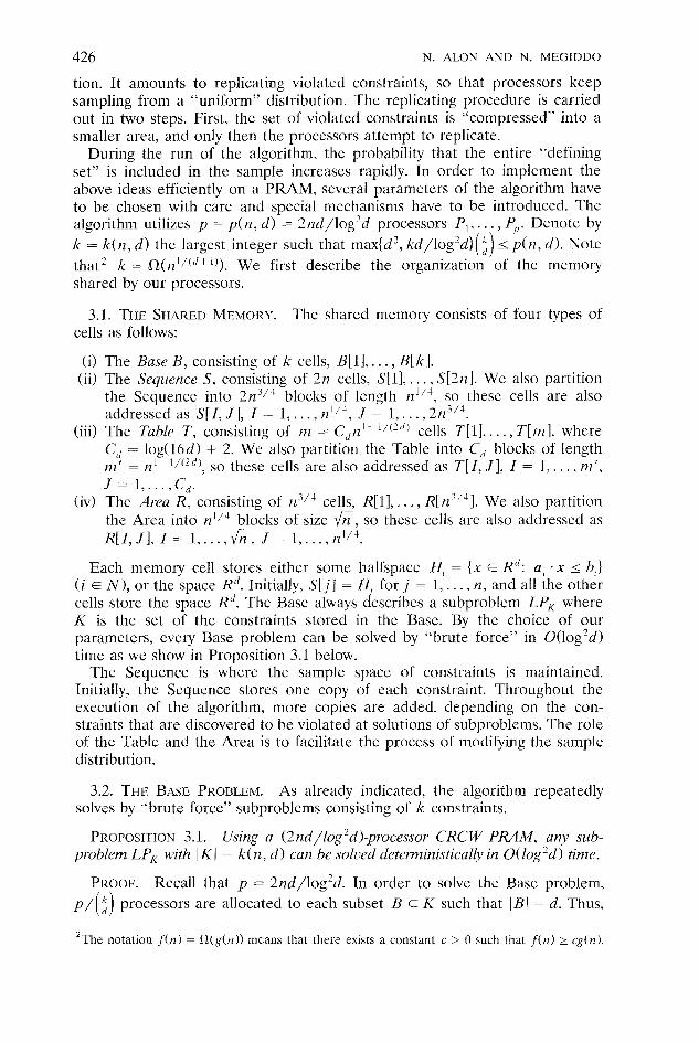
tion. It amounts to replicating violated constraints, so that processors keep sampling from a "uniform" distribution. The replicating procedure is carried out in two steps. First, the set of violated constraints is "compressed" into a smaller area, and only then the processors attempt to replicate.

During the run of the algorithm, the probability that the entire "defining set" is included in the sample increases rapidly. In order to implement the above ideas efficiently on a PRAM, several parameters of the algorithm have to be chosen with care and special mechanisms have to be introduced. The algorithm utilizes p = p(n , d ) = 2nd/log2d processors P,, . . . , P,,. Denote by k = k(n, d ) the largest integer such that rnax{d3, kd/log2d)(i) I p(ri, d). Note that2 k = fl(nl/"'+ "1. We first describe the organization of the memory shared by our processors.

3.1. THE SHARED MEMORY. The shared memory consists of four types of cells as follows:

(i) The Base B, consisting of k cells, B[ll, . . . , B[kl. (ii) The Sequence S. consisting of 2n cells, S[1], . . . , S[2rz]. We also partition

the Sequence into 2n3/"locks of length n'/" so these cells are also addressed as S[I, J] , I = 1, . . . , ~ z " ~ , J = 1,. . . , 2n3/'.

(iii) The Table T, consisting of m = C,n1-'"2d' cells T[1], . . . , T[nz], where C, = log(l6d) + 2. We also partition the Table into C, blocks of length m' = n 1 1 / ( 2 d ' , SO these cells are also addressed as T [ I , J], I = 1,. . . , nz', J = 1, . . . , Cd.

(iv) The Area R, consisting of n3/' cells, R[1], . . . , ~[n" ' ] . We also partition the Area into n 'I4 blocks of size 6, so these cells are also addressed as R[I, J] , I = 1,. . . ,6, J = 1, . . . , H ' / ~ .

Each memory cell stores either some halfspace H, = {x E R,: a, .X I 6,) (i E N ) , or the space Rd. Initially, S[j] = HI for j = 1,. . . ,P I , and all the other cells store the space R". The Base always describes a subproblem LP, where K is the set of the constraints stored in the Base. By the choice of our parameters, every Base problem can be solved by "brute force" in 0(log2d) time as we show in Proposition 3.1 below.

The Sequence is where the sample space of constraints is maintained. Initially, the Sequence stores one copy of each constraint. Throughout the execution of the algorithm, more copies are added, depending on the con- straints that are discovered to be violated at solutions of subproblems. The role of the Table and the Area is to facilitate the process of modifying the sample distribution.

3.2. THE BASE PROBLEM. AS already indicated, the algorithm repeatedly solves by "brute force" subproblems consisting of k constraints.

PROPOSITION 3.1. Using a (2nd/log'd)-processor CRCW PRAM, any sub- problem LP, with IK( = k ( n , d) call be solrwd deternzirzistica1l)'in O(log%) time.

PROOF. , \ Recall that p = 2nd/log2d. In order to solve the Base problem, p / ( : ) processors are allocated to each subset B c K such that IBI = d. Thus,

ha he notation f ( n ) = bl(g(r2)) means that there exists a constant c > 0 such that f(rz) r cg(n) .

Linear Programming in Constant Time 427

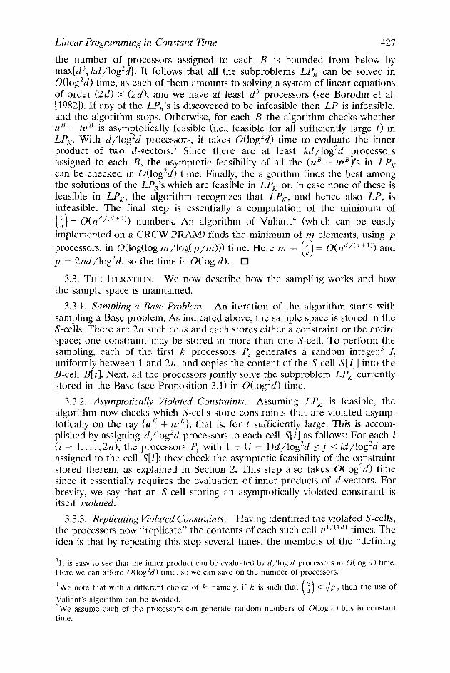
the number of processors assigned to each B is bounded from below by max{d3, kd/log%}. It follows that all the subproblems LP, can be solved in 0(log2d) time, as each of them amounts to solving a system of linear equations of order (2d) x (2d), and we have at least d 3 processors (see Borodin et al. [1982]). If any of the LPB7s is discovered to be infeasible then L P is infeasible, and the algorithm stops. Otherwise, for each B the algorithm checks whether uB + tvR is asymptotically feasible (i.e., feasible for all sufficiently large t) in LPK. With d/log% processors, it takes 0(log2d) time to evaluate the inner product of two d-vectors.' Since there are at least kd/log" processors assigned to each B7 the asymptotic feasibility of all the (uR + tvB)'s in LP, can be checked in 0(log2d) time. Finally, the algorithm finds the best among the solutions of the LPB7s which are feasible in LP, or, in case none of these is feasible in LP,, the algorithm recognizes that LP,, and hence also LP, is infeasible. The final step is essentially a computation of the minimum of (:) = ~ ( n * / ( ' ' ' ~ ) ) numbers. An algorithm of valiant4 (which can be easily implemented on a CRCW PRAM) finds the minimum of m elements, using p processors, in O(log(1og m/log(p/m))) time. Here m = (5) = O(nd/(dil)) and p = 2rzd/log2d, so the time is O(1og d).

3.3. THE ITERATION. We now describe how the sampling works and how the sample space is maintained.

3.3.1. Sampling a Base Problem. An iteration of the algorithm starts with sampling a Base problem. As indicated above, the sample space is stored in the S-cells. There are 211 such cells and each stores either a constraint or the entire space; one constraint may be stored in more than one S-cell. To perform the sampling, each of the first k processors P, generates a random integer5 Ii uniformly between 1 and 2n, and copies the content of the S-cell S[I,] into the B-cell B[i]. Next, all the processors jointly solve the subproblem LP, currently stored in the Base (see Proposition 3.1) in 0(log2d) time.

3.3.2. Asymptotically Violated Constraints. Assuming LP, is feasible, the algorithm now checks which S-cells store constraints that are violated asymp- totically on the ray {u" + tu"), that is, for t sufficiently large. This is accom- plished by assigning d/log2d processors to each cell S[i] as follows: For each i ( i = 1,. . . ,2n), the processors P, with 1 + ( i - l)d/log2d r j I id/log% are assigned to the cell S[i]; they check the asymptotic feasibility of the constraint stored therein, as explained in Section 2. This step also takes 0(log2d) time since it essentially requires the evaluation of inner products of d-vectors. For brevity, we say that an S-cell storing an asymptotically violated constraint is itself rliolated.

3.3.3. Replicating Violated Constraints. Having identified the violated S-cells, the processors now "replicate" the contents of each such cell times. The idea is that by repeating this step several times, the members of the "defining

3 ~ t is easy to see that the inner product can be evaluated by d/log d processors in O(log d ) time. Here we can afford 0(log2d) time. so we can save on the number of processors.

'we note that with a different choice of k, namely. if k is such that (I) a 6, then the use of ~,

Valiant's algorithm can be avoided. 'we assume each of the processors can generate random numbers of O(log 1 1 ) bits in constant time.

428 N. ALON AND N. MEGIDDO

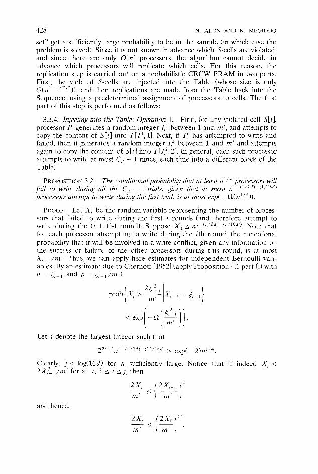
set" get a sufficiently large probability to be in the sample (in which case the problem is solved). Since it is not known in advance which S-cells are violated, and since there are only O(n) processors, the algorithm cannot decide in advance which processors will replicate which cells. For this reason, the replication step is carried out on a probabilistic CRCW PRAM in two parts. First, the violated S-cells are injected into the Table (whose size is only O ( I Z ' - ' / ( ~ ~ ) ) ) , and then replications are made from the Table back into the Sequence, using a predetermined assignment of processors to cells. The first part of this step is performed as follows:

3.3.4. Injecting into the Table: Operation 1. First, for any violated cell S[i], processor P, generates a random integer I,' between 1 and m', and attempts to copy the content of S[i] into TIIll, 11. Next, if P, has attempted to write and failed, then it generates a random integer I,' between 1 and 171' and attempts again to copy the content of S [ i ] into T[I,< 21. In general, each such processor attempts to write at most C, - 1 times, each time into a different block of the Table.

PROPOSITION 3.2. The conditiorlnlprobability that at least r ~ ' / ~ processors will fail to write during all the C,, - 1 trials, given that at most n'-('/2d)-('/'6d' processors attempt to write during the first trial, is at most e,xp( - fl(n'/4)).

PROOF. Let XI be the random variable representing the number of proces- sors that failed to write during the first i rounds (and therefore attempt to write during the ( i + 1)st round). Suppose X,, I n'-"/"d"'/16d'). Note that for each processor attempting to write during the ith round, the conditional probability that it will be involved in a write conflict, given any information on the success or failure of the other processors during this round, is at most X,- , /mt . Thus, we can apply here estimates for independent Bernoulli vari- ables. By an estimate due to Chernoff [I9521 (apply Proposition 4.1 part (i) with n = tl-, and p = (I-,/rnl),

Let j denote the largest integer such that

Clearly, j < log(16ri) for n sufficiently large. Notice that if indeed XI I 2 x,:, /nzf for all i, 1 I i I j, then

and hence,

Linear Programming itz Constant Time 429

Thus, X I - < 22J-'n1-(1/"d'-("~16*~. The probability that j does not satisfy the latter is at most e~p( - f l (n ' /~ ) ) . Combining this with Proposition 4.1 part (ii), we get

We note that, as pointed out by one of the referees, the analysis in the last proposition can be somewhat simplified by having the processors try to inject the violated constraints to the same table for some C& times (or until they succeed). It is easy to see that for, say, Ch = 16d the conclusion of Proposition 3.2 will hold. However, this will increase the running time of each phase of our algorithm to fl(d) and it is therefore better to perform the first part of the injection as described above. Alternatively, the time increase can be avoided by making all C& attempts in parallel and then, in case of more than one success, erase all but the first successful replication. We omit the details of the implementation.

3.3.5. Injecting into the Table: Operation 2. To complete the step of inject- ing into the Table, one final operation has to be performed. During this operation, the algorithm uses a predetermined assignment of some q = n114 processors to each of the 2n314 S-blocks, for example, processor P, is assigned to the block S[*, [jn-1/4]]. An S-cell is said to be actirle at this point if it has failed C, - 1 times to be injected into the Table. An S-block is said to be actiue if it contains at least one active cell.' For each active block S[*, Jl (1 I J I 2n314), all the q processors assigned to S[ *, J l attempt to write the symbol J into the Area R as follows: The ith processor among those assigned to S[*, J ] generates a random7 integer I, between 1 and 6 , and attempts to write the symbol J into the cell R[I,, i].

PROPOSITION 3.3. If there are less than nl/' actirle S-blocks, then the probabil- ity that write conflicts will occur in euey single R-block is less than exp( - R(nl/"):

PROOF. At most nl/' processors attempt to write into any R-block (whose ,

length is 6 ) , so the probability of a conflict within any fixed R-block is less than 1/2. Thus, the probability of conflicts in every single R-block is less than 2-n1/4. 0

It takes constant time to reach a situation where all the processors recognize that a specific block R[*, J*] was free of conflict (assuming at least one such block exists). At this point, the names of all the active S-blocks have been moved into one commonly known block R[*, J*]. The role of the area R is to facilitate the organization of the work involved in replicating the remaining active S-blocks into the last T-block.

Next, n114 processors are assigned to each cell R[I, J* ] ( I = 1,. . . , 6 ) . Each such cell is either empty or contains the index J, of some active S-block S[*, J,]. In the latter case, the processors assigned to R[I, J*] copy the contents of the active cells of S[*, J,] into the last T-block, T[* Cd], according to some predetermined assignment.

'1t takes constant time to reach the situation where each of the q processors knows whether or not it is assigned to an active S-block. 7 ~ h i s last step can also be done deterministically with hash functions.

430 N. ALON AND N. MEGIDDO

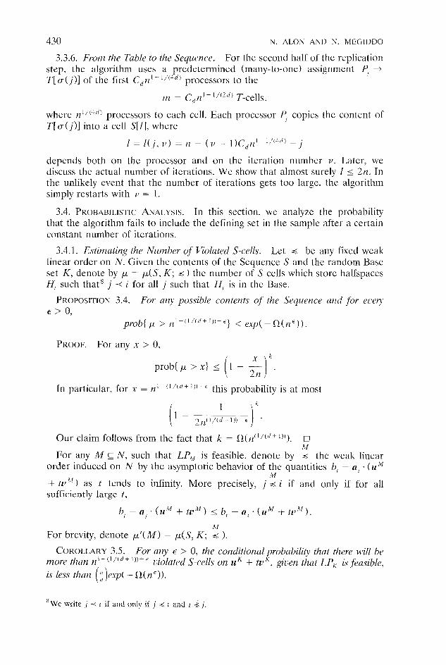
3.3.6. From the Table to the Sequence. For the second half of the replication step, the algorithm uses a predetermined (many-to-one) assignment P, +

T [ a ( j ) ] of the first cdn- 'I"" processors to the

where i ~ ' / " ~ ' processors to each cell. Each processor P, copies the content of T [ a ( j ) ] into a cell S[ I ] , where

depends both on the processor and on the iteration number v . Later, we discuss the actual number of iterations. We show that almost surely 1 5 2n. In the unlikely event that the number of iterations gets too large, the algorithm simply restarts with v = 1.

3.4. PROBABILISTIC ANALYSIS. In this section. we analyze the probability that the algorithm fails to include the defining set in the sample after a certain constant number of iterations.

3.4.1. Estimating the Number of Violated S-cells. Let s be any fixed weak linear order on N. Given the contents of the Sequence S and the random Base set K, denote by p = p(S , K ; s the number of S-cells which store halfspaces H, such that" j i for all j such that HI is in the Base.

PROPOSITION 3.4. For any possible contents of the Sequence ~ lnd for e ~ w y E > 0,

pl.ob{ f i > n~ - ( I / i d+ I ) ) + ' } < exp(-!2(tze)) .

PROOF. For any x > 0,

Our claim follows from the fact that k = f l ( r l " / ( d + I) ' ) . [7 hl

For any M c N, such that LP, is feasible, denote by s the weak linear order induced on N by the asymptotic behavior of the quantities b, - a, - ( u M

M + tzjn' as t tends to infinity. More precisely, j s i if and only if for all sufficiently large t ,

b, - a , . (u" + t ~ l ~ ' ) bl - a [ . ( u M + tu").

hi For brevity, denote p f ( M ) = P(S, K; s ).

COROLLARY 3.5. For any E > 0, the conditional probability that there will be more than n ' - ( l / ( d t l ) ) t ' violated S-cells on u + tv", gillen that LP, is feasible, is less than (;)erp( - ~ ( n ' ) ) .

%e write J < I if and only if J s 1 and I 4 j .

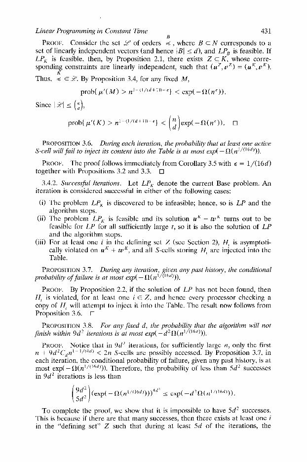
Linear Programming in Constant Time 43 1 R

PROOF. Consider the set 2 of orders 2 , where B c N corresponds to a set of linearly independent vectors (and hence IBI 5 d), and LP, is feasible. If LP, is feasible, then, by Proposition 2.1, there exists Z c K, whose corre- sponding constraints are linearly independent, such that (uZ,uZ) = (uK,uK).

K

Thus, s €2'. By Proposition 3.4, for any fixed M,

PROPOSITION 3.6. Dzwing each iteration, the probability that at least one acti~le S-cell will fail to inject its content into the Table is at most exp( - lR(n1/(16d))).

PROOF. The proof follows immediately from Corollary 3.5 with E = 1/(16d) together with Propositions 3.2 and 3.3.

3.4.2. Sz~cessfitl Iterations. Let LP, denote the current Base problem. An iteration is considered successful in either of the following cases:

(i) The problem LP, is discovered to be infeasible; hence, so is LP and the algorithm stops.

(ii) The problem LP, is feasible and its solution u" + tu" turns out to be feasible for LP for all sufficiently large t, so it is also the solution of LP and the algorithm stops.

(iii) For at least one i in the defining set Z (see Section 2), H, is asymptoti- cally violated on u" + tvK, and all S-cells storing H, are injected into the Table.

PROPOSITION 3.7. During any iteration, given any past histo y, the conditional probability of failure is at most exp( - i2(n1/(16d))).

PROOF. By Proposition 2.2, if the solution of LP has not been found, then H, is violated, for at least one i E Z, and hence every processor checking a copy of H, will attempt to inject it into the Table. The result now follows from Proposition 3.6. 0

PROPOSITION 3.8. For any fixed d, the probability that the algorithm will not finish within 9d iterations is at most exp( - d fl(n1/(16d))).

PROOF. Notice that in 9d"terations, for sufficiently large n, only the first n + 9d'Cdn'-'/(4d) < 211 S-cells are possibly accessed. By Proposition 3.7, in each iteration, the conditional probability of failure, given any past history, is at most exp( - i2(n'/('6d))). Therefore, the probability of less than 5d2 successes in 9d2 iterations is less than

To complete the proof, we show that it is impossible to have 5d%uccesses. This is because if there are that many successes, then there exists at least one i in the "defining set" Z such that during at least 5d of the iterations, the

432 N . ALON AND N. MEGIDDO

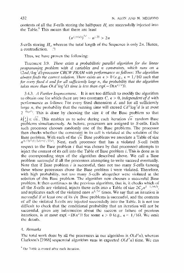
contents of all the S-cells storing the halfspace H, are successfully injected into the able.^ This means that there are least

S-cells storing H,, whereas the total length of the Sequence is only 211. Hence, a contradiction. 0

Thus, we have proven the following:

THEOREM 3.9. There exists a probabilistic parallel algorithm for the linear programniizg problem with d uariables and 11 constraints, which nins on a (2nct/log2d)-processor CRCW PRAM with pe$onnance as follows: The algorithm always finds the correct solution. There exists an E > 0 (e.g., E = 1 / 1 6 ) such that for eceiy fzed d and for all s~ij$icieiztly large n , the probability that the algorithm takes more than 0(d"og%) time is less than exp( - f l ( n ' / d ) ) .

3.4.3. A Further Improvement. It is not too difficult to modify the algorithm to obtain one for which there are two constants C, E > 0, independent of d with performance as follows: For every fixed dimension d, and for all sufficiently large n , the probability that the running time will exceed Cdqog2d is at most 2 ~ ~ ' ~ ' ' . This is done by choosing the size k of the Base problem so that

k ( : 5 6. This enables us to solve during each iteration 6 random Base pro b lems simultaneously. As before, processors are assigned to S-cells. Each such processor chooses randomly one of the Base problems. The processor then checks whether the constraint in its cell is violated at the solution of the Base problem. With each of the 6 Base problems we associate a Table of size i z c1 '2 )Pc ' /2d )+(1 /32d) . Next, each processor that has a violated S-cell (with respect to the Base problem i that was chosen by that processor) attempts to inject the content of its cell into the Table of Base problem i. This is done as in the corresponding steps of the algorithm described above. We call a Base problem successfir1 if all the processors attempting to write succeed eventually. Note that if Base problem i is successful, then not too many S-cells (among those whose processors chose the Base problem i were violated. Therefore, with high probability, not too many S-cells altogether were violated at the solution of this Base problem. The algorithm now chooses a successful Base problem. It then continues as the previous algorithm, that is, it checks which of all the S-cells are violated, injects these cells into a Table of size 2 C , , 1 ~ ~ ' / ( ~ ~ ) , and replicates each of the violated ones r 1 ' / 5 d times. We say that an iteration is szrccessjiil if at least one of its fi Base problems is successful, and the contents of all the violated S-cells are injected successfully into the Table. It is not too difficult to check that the conditional probability that an iteration will not be successful, given any information about the success or failure of previous iterations, is at most exp( - f l ( n E ) ) for some E > 0 (e.g., E = 1/16). We omit the details.

4. Remarks

The total work done by all the processors in our algorithm is 0 ( d 3 n ) , whereas Clarkson's [I9881 sequential algorithm runs in expected 0 ( d 2 n ) time. We can

he Table is erased after each iteration.

Linear Programming in Constant Time 433

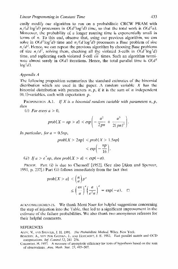
easily modify our algorithm to run on a probabilistic CRCW PRAM with n/(d log2dd) processors in 0(d310g%) time, so that the total work is 0(d2n) . Moreover, the probability of a longer running time is exponentially small in terms of n. To this end, observe that, using our previous algorithm, we can solve in 0(d210g2d) time and n/(d log'd) processors a Base problem of size n/d< Hence, we can repeat the previous algorithm by choosing Base problems of size n/d2, solving them, checking all the violated S-cells in 0(d210g%d) time, and replicating each violated S-cell 6 times. Such an algorithm termi- nate almost surely in O(d) iterations. Hence, the total parallel time is 0 ( d 3 log 'dl.

Appendix A

The following proposition summarizes the standard estimates of the binomial distribution which are used in the paper. A random variable X has the binomial distribution with parameters n , p , if it is the sum of n independent (0, lbvariables, each with expectation p.

PROPOSITION A.1. If X is a binomial random variable with parameters n, p , then

(i) For euey a > 0,

a prob{X - rip > a} < exp

In particular, for a = OSnp,

(ii) If a > e2np, then prob{X > a) < exp( -a).

PROOF. Part (i) is due to Chernoff [1952]. (See also [Alon and Spencer, 1991, p. 2371.) Part (ii) follows immediately from the fact that

ACKNOWLEDGMENTS. We thank Moni Naor for helpful suggestions concerning the step of injection into the Table, that led to a significant improvement in the estimate of the failure probabilities. We also thank two anonymous referees for their helpful comments.

REFERENCES ALON, N., AND SPENCER, J. H. 1991. The Probabilistic Method. Wiley, New York. BORODIN, A,, VON ZUR GATHEN, J.. AND HOPCROFT, J. E. 1982. Fast parallel matrix and GCD

computations. Znf . Control 52, 241-256. CHERNOPF, H. 1952. A measure of asymptotic efficiency for tests of hypothesis based on the sum

of observations. Ann. Math. Stat. 23, 493-507.

434 N. ALON AND N. MEGIDDO

CLARKSON, K. L. 1986. Linear programming in 0(113''~) time. Inf. Proc. Lett. 2-7, 21-24. CLARKSON, K. L. 1988. Las Vegas algorithms for linear and integer programming when the

dimension is small. Unpublished manuscript. (A preliminary version appeared in Proceedings of the 29th rlrzn~~nl IEEE Symposium on Foundations of Computer Science. IEEE. New York, pp. 452-4561,

DENG, X. An optimal parallel algorithm for linear programming in the plane. Unpublished manuscript.

DYER, M. E. 1986. On a multidimensional search technique and its application to the Euclidean one-center problem. SIAM J. Comput. 15, 725-738.

DYER, M. E., AND FREEZE, A. M. 1989. A randomized algorithm for fixed dimensional linear programming. Math. Prog. 44, 203-2 12.

LUEKER, G. S., MEGIDDO, N., AND RAMACHANDRAN, V. 1990. Linear programming with two variables per inequality in poly log time. S U M J. Comput. 19, 1000-1010.

MEGIDDO, N. 1952. Parallel algorithms for finding the maximum and the median almost surely in constant-time. Tech. Rep. Graduate School of Industrial Administration, Carnegie-Mellon Univ., Pittsburgh, Pa., (Oct.).

MEGIDDO, N. 1953. Linear programming in linear time when the dimension is fixed. J. ACM31, 114-127.

REISCHUK, R. 1981. A fast probabilistic parallel sorting algorithm. In Proceedings of the 2 n d Annual IEEE Symposzr~t~~ on Foundatrons of Computer Science. IEEE, New York, pp. 711-219.

VALIANT, L. G. 1975. Parallelism in comparison algorithms. S U M J. Comput. 4, 348-355. WELZL., E. 1988. Partition trees for triangle counting and other range search problems. In

Proceedings of the 4th A n n ~ ~ a l A c M S,vrnposiunt on Comp~~tational Geomet~y (Urbana-Champaign, Ill.. June 6-8). ACM, New York, pp. 23-33.

fournal of the Assoc~dtlon for Computlng Mdchlnery, Vol 41. No 2. March I Y Y 4