CENTER FOR

MACHINE PERCEPTION

CZECH TECHNICAL

UNIVERSITY

RESEARCH

REPO

RT

ISSN

1213-2

365

Parallel MRI Reconstruction Using

B-splines

Jan Petr, Jan Kybic, Vaclav Hlavac

petrj5@cmp.felk.cvut.cz

CTU–CMP–2004–09Published also as: K333–19/04

August 30, 2004

Available atftp://cmp.felk.cvut.cz/pub/cmp/articles/petr/Petr-TR-2004-09.pdf

Supervisor: Jan Kybic, Vaclav Hlavac

The 1st author was supported by the STINT under project DurIG2003-2 062 and by the Austrian Ministry of Education underproject CONEX GZ 45.535, the 2nd author was supported by theAustrian Ministry of Education under project CONEX GZ 45.535,the 3rd author was supported by the European Union under projectIST-2001-32184 and by the Czech Ministry of Education underproject LN00B096 and by the STINT under project Dur IG2003-2 062 and by the Austrian Ministry of Education under projectCONEX GZ 45.535.

Research Reports of CMP, Czech Technical University in Prague, No. 9, 2004

Published by

Center for Machine Perception, Department of CyberneticsFaculty of Electrical Engineering, Czech Technical University

Technicka 2, 16627 Prague 6, Czech Republicfax +4202 24357385, phone +4202 24357637, www: http://cmp.felk.cvut.cz

The purpose of this document is to summarize the current state of our work on areconstruction algorithm for parallel MRI. This summary should be used describe ourwork to Dr. Michael Bock from the research group “Interventional Methods” in theDepartment for Medical Physics in Radiology in Deutsches Krebsforschungszentrum,Heidelberg which we collaborate with.

1 Introduction

Parallel MRI is used to increase the speed of the MRI acquisition. Simultaneously usingmore coils (array coils) with distinct spatial sensitivities enables to acquire more datain a single scan. Consequently it is possible to sample more sparsely in k-space andthis way to speed up the acquisition. The decrease of data amount due to the sparsersampling is compensated by the use of several coils. The full-resolution image can bereconstructed from a set of low-resolution images from the array coils with only a neglibleloss in quality.

The main goals of our work are to propose and implement a better and faster algo-rithm than the currently available reconstruction algorithms - SMASH [7], SENSE [4]and their advanced versions.

Our aim is to increase the speed of the reconstruction, make it robust to noise andimprove the quality of the reconstruction. The idea is to approximate the coefficientsof the reconstruction matrix using B-spline functions [8]. This reduces the number ofparameters which need to be estimated and the estimation process is thus faster.

The knowledge of the basic MRI principles is recommended for easier understandingof this paper. For the MRI basics, we refer the reader to literature [5, 9].

2 Parallel MRI

In standard MRI, a single coil with an approximately homogeneous spatial sensitivity(a body coil) is used to retrieve the images. In parallel MRI (pMRI), several receivercoils (array coils) with distinct spatial sensitivities are used simultaneously. Therefore,image points have distinct intensity values in the image from each of the array coils.This brings an additional information about the spatial position.

Let us have a closer look on what is happening during the acquisition. We willassume that the unaliased (full density sampled) body coil image S is identical to thereal object and its ideal reconstruction (we neglect noise in the body coil).

The image Sl from the l-th array coil is therefore modeled as the body-coil imagemodulated by the coil sensitivity

Sl(x,y) = Cl(x,y)S(x,y), (1)

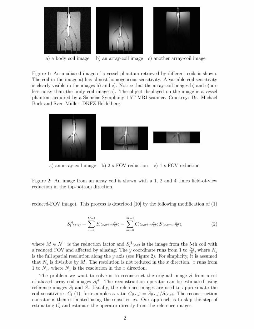
where Cl is the sensitivity map of the l-th coil (see Figure 1).

Reducing the field-of-view (sensed size of the imaged area) of the acquisition (i.e.,sparser sampling in the k-space) causes an aliasing. The reason is that the whole slicehas been excited by an RF-pulse and the points outside the field-of-view (FOV) aremisinterpreted by aliasing as being inside. However, the imaged area gets smaller as aneffect of the sparser sampling in the k-space and the parts of the image that were cut offsuperimpose over the image causing the aliasing (the image is called an aliased image or

1

a) a body coil image b) an array-coil image c) another array-coil image

Figure 1: An unaliased image of a vessel phantom retrieved by different coils is shown.The coil in the image a) has almost homogeneous sensitivity. A variable coil sensitivityis clearly visible in the images b) and c). Notice that the array-coil images b) and c) areless noisy than the body coil image a). The object displayed on the image is a vesselphantom acquired by a Siemens Symphony 1.5T MRI scanner. Courtesy: Dr. MichaelBock and Sven Muller, DKFZ Heidelberg.

a) an array-coil image b) 2 x FOV reduction c) 4 x FOV reduction

Figure 2: An image from an array coil is shown with a 1, 2 and 4 times field-of-viewreduction in the top-bottom direction.

reduced-FOV image). This process is described [10] by the following modification of (1)

SAl (x,y) =

M−1∑

m=0

Sl(x,y+mNyM

) =

M−1∑

m=0

Cl(x,y+mNyM

) S(x,y+mNyM

), (2)

where M ∈ N+ is the reduction factor and SAl (x,y) is the image from the l-th coil with

a reduced FOV and affected by aliasing. The y coordinate runs from 1 to Ny

M, where Ny

is the full spatial resolution along the y axis (see Figure 2). For simplicity, it is assumedthat Ny is divisible by M . The resolution is not reduced in the x direction. x runs from1 to Nx, where Nx is the resolution in the x direction.

The problem we want to solve is to reconstruct the original image S from a setof aliased array-coil images SA

l . The reconstruction operator can be estimated usingreference images Sl and S. Usually, the reference images are used to approximate thecoil sensitivities Cl (1), for example as ratio Cl(x,y) = Sl(x,y)/S(x,y). The reconstructionoperator is then estimated using the sensitivities. Our approach is to skip the step ofestimating Cl and estimate the operator directly from the reference images.

2

2.1 SENSE and SMASH

Currently, there are several methods for reconstructing of a full field-of-view image.Most of them are based on one of the two methods called SENSE [4] and SMASH [7]. InSENSE, it is assumed that the modulation by the sensitivity and the aliasing are bothlinear transformations. Therefore the reconstruction transformation is also linear andit can be computed as an inversion of the composite transformation of the aliasing andsensitivity transformations.

The SMASH works in the frequency domain. A linear combination of sensitivity pro-files is fitted to a harmonic function. The corresponding linear transformation is appliedto array-coil images in the Fourier domain, which causes a phase shift according to theused harmonic function. This way, the shifted lines in the Fourier domain approximatethe ommited lines in k-space. An image without aliasing can be reconstructed.

Please note that this is only a brief description of the basic techniques. For more de-tailed description of the currently-used methods please see the articles about GRAPPA [2],VD-AUTO-SMASH [1], Tailored SMASH [6] and Self-calibrating parallel imaging [3]methods.

3 Direct estimation of the reconstruction matrix co-

efficients using B-splines

A method that estimates the coefficients directly from retrieved images using B-splinesis described in this section. First, we introduce the terminology, the assumptions andthe main idea of the method. The following subsections include the detailed descriptionof the reconstruction method.

Several images are needed for the estimation step (we will call them reference images):an unaliased body-coil image S and a set of unaliased array-coil images Sl. All thereference images must display the same object.

The set of aliased array-coil images needed for the subsequent reconstruction willbe called input images. They do not have to display the same object as the referenceimages, but must be acquired with the same coil configuration. We then reconstruct animage S as an approximation of how an unaliased image of the input object would looklike if displayed by the body coil (i.e., our ideal reconstruction).

We will estimate the reconstruction operator directly from the reference images Sand SA

l in such a way as to minimize the square difference reconstruction error (l2 error=∑

x,y(S(x,y) − S(x,y))2).

It is clear that after the acquisition of the reference images and estimation all the fol-lowing acquisitions can be performed much faster as there is no need for more calibrationscans.

3.1 General method description

As stated in (2), aliased array-coil images SAl are linearly transformed versions of the

original image S. We are assuming invertibility of the transformation. This is possi-ble with a reasonable coil configuration (the sensitivity maps should be distinct fromeach other and for each part of the FOV there must be at least one coil that receivesenough signal from it). The inverse transformation could be written as a pixelwise linear

3

combination of aliased images (with weights α)

S(x,y+mNyM

) =

L∑

l=1

αlm(x,y) SAl (x,y), (3)

where αlm(x,y) ∈ R are the weights for the l-th coil at points y = 1, 2, . . . , Ny

M, x =

1, 2, . . . , Nx and m = 0, . . . , M − 1.Lets incorporate the fact, that each pixel in the aliased array-coil image SA

l is asuperposition of M pixels from the array-coil image Sl (2), into (3)

S(x,y+mNyM

) =L∑

l=1

αlm(x,y)

M−1∑

m′=0

Sl(x,y+m′ NyM

) =M−1∑

m′=0

L∑

l=1

αlm(x,y) Sl(x,y+m′ NyM

).

The coefficients should be estimated in order to fulfil the condition that the valueS(x,y+m

NyM

) is independent of the values Sl(x,y+m′ NyM

) for m 6= m′ (because they displaydistinct parts of the imaged object). Thus the coefficients α should meet the conditionsof orthogonality (see Figure 3)

L∑

l=1

αlm(x,y) Sl(x,y+m′ NyM

) =

{

S(x,y+mNyM

) for m = m′

0 for m 6= m′ . (4)

This idea can be verified by estimating the coefficients for a reference object Sr. Thereconstruction will be performed using an input object S i which is different from Sr butwas acquired using the same coil configuration. We shall use the following notation:Sr, Sr

l are the reference images and Cl is the coil sensitivity that is the same for bothreference and input images. Coefficients are estimated according to equation (4) andsubstituting the array-coil images by a product of the body-coil image and the coilsensitivity (1).

L∑

l=1

αlm(x,y) Srl (x,y) =

L∑

l=1

αlm(x,y) Sr(x,y+m′ Ny

M) Cl(x,y+m′ Ny

M) =

{

Sr(x,y+mNyM

) for m = m′

0 for m 6= m′ .

The image value Sr(x, y) can be extracted from the sum and divided out of theequation. It becomes visible that the reconstruction coefficients are estimated from thecoil sensitivities although the sensitivity maps are not included in the estimation stepexplicitly

L∑

l=1

αlm(x,y) Cl(x,y+m′ NyM

) =

{

1 for m = m′

0 for m 6= m′ .

The following equation shows that the condition (4) assumes a perfect reconstruction ofan object Si

L∑

l=1

αlm(x,y) SAil (x,y) =

L∑

l=1

αlm(x,y)

M−1∑

m′=0

Sil (x,y+m′ Ny

M) =

L∑

l=1

αlm(x,y)

M−1∑

m′=0

Si(x,y+m′ Ny

M) Cl(x,y+m′ Ny

M) =

= Si(x,y+m

NyM

)

L∑

l=1

αlm(x,y) Cl(x,y+mNyM

) +∑

m′ 6=m

Si(x,y+m′ Ny

M)

L∑

l=1

αlm(x,y) Cl(x,y+m′ NyM

) =

= Si(x,y+m

NyM

) · 1 +∑

m′ 6=m

Si(x,y+m′ Ny

M) · 0 = Si

(x,y+mNyM

).

where SAil are the aliased input images. Si

l and Si are unaliased images of the inputobject. Si

l and Si are not available for the reconstruction.

4

PSfrag replacements

Sl(1)

Sl(2)

αl(1)

αl(1)

αl(1)

αl(2)

αl(2)

αl(2)

S(1)

S(2)

S(1)

S(2)

Sl(1) + Sl(2)

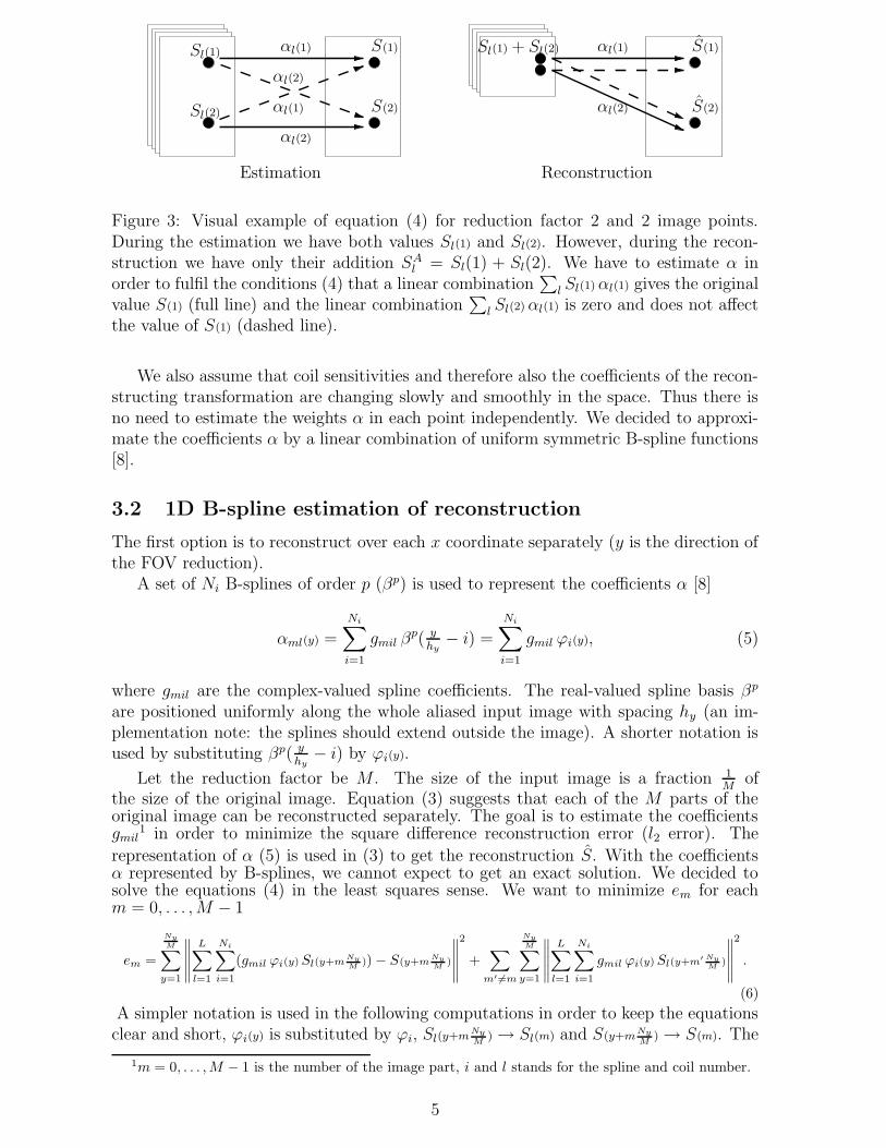
Estimation Reconstruction

Figure 3: Visual example of equation (4) for reduction factor 2 and 2 image points.During the estimation we have both values Sl(1) and Sl(2). However, during the recon-struction we have only their addition SA

l = Sl(1) + Sl(2). We have to estimate α inorder to fulfil the conditions (4) that a linear combination

∑

l Sl(1) αl(1) gives the originalvalue S(1) (full line) and the linear combination

∑

l Sl(2) αl(1) is zero and does not affectthe value of S(1) (dashed line).

We also assume that coil sensitivities and therefore also the coefficients of the recon-structing transformation are changing slowly and smoothly in the space. Thus there isno need to estimate the weights α in each point independently. We decided to approxi-mate the coefficients α by a linear combination of uniform symmetric B-spline functions[8].

3.2 1D B-spline estimation of reconstruction

The first option is to reconstruct over each x coordinate separately (y is the direction ofthe FOV reduction).

A set of Ni B-splines of order p (βp) is used to represent the coefficients α [8]

αml(y) =

Ni∑

i=1

gmil βp( y

hy− i) =

Ni∑

i=1

gmil ϕi(y), (5)

where gmil are the complex-valued spline coefficients. The real-valued spline basis βp

are positioned uniformly along the whole aliased input image with spacing hy (an im-plementation note: the splines should extend outside the image). A shorter notation isused by substituting βp( y

hy− i) by ϕi(y).

Let the reduction factor be M . The size of the input image is a fraction 1M

ofthe size of the original image. Equation (3) suggests that each of the M parts of theoriginal image can be reconstructed separately. The goal is to estimate the coefficientsgmil

1 in order to minimize the square difference reconstruction error (l2 error). The

representation of α (5) is used in (3) to get the reconstruction S. With the coefficientsα represented by B-splines, we cannot expect to get an exact solution. We decided tosolve the equations (4) in the least squares sense. We want to minimize em for eachm = 0, . . . , M − 1

em =

Ny

M∑

y=1

∥

∥

∥

∥

∥

L∑

l=1

Ni∑

i=1

(gmil ϕi(y) Sl(y+mNyM

)) − S(y+mNyM

)

∥

∥

∥

∥

∥

2

+∑

m′ 6=m

Ny

M∑

y=1

∥

∥

∥

∥

∥

L∑

l=1

Ni∑

i=1

gmil ϕi(y) Sl(y+m′ NyM

)

∥

∥

∥

∥

∥

2

.

(6)

A simpler notation is used in the following computations in order to keep the equationsclear and short, ϕi(y) is substituted by ϕi, Sl(y+m

NyM

) → Sl(m) and S(y+mNyM

) → S(m). The

1m = 0, . . . , M − 1 is the number of the image part, i and l stands for the spline and coil number.

5

other simplifications are similar to the mentioned ones. The operator ∗ is a complexconjugate. Note the basis of the B-splines ϕ is real.

Lets substitute the absolute value of complex numbers with another interpretation(‖z‖2

= zz∗) into the reconstruction error (6)

em =∑

y

{(

∑

l,i

(gmil ϕi Sl(m)) − S(m)

)(

∑

l,i

(g∗mil ϕi S

∗l (m)) − S∗

(m)

)

+∑

m′ 6=m

{(

∑

l,i

gmil ϕi Sl(m′)

)(

∑

l,i

g∗mil ϕi S

∗l (m′)

)}}

(7)

In order to minimize the error em expressed in (7), we consider em(gmil, g∗mil) to be a func-

tion of gmil and g∗mil and calculate the derivatives for g∗

mil for each i and l and set themequal to zero

0 = ∂em

∂g∗mil

0 =∑

y

∑

i′,l′

gmi′l′ ϕi′ Sl′(m) − S(m)

ϕi S∗l (m)+

+∑

m′ 6=m

∑

i′,l′

gmi′l′ ϕi′ Sl′(m′)

ϕi S∗l (m′)

∑

y

ϕi S∗l (m) S(m) =

∑

y

∑

i′,l′

gmi′l′ ϕi′ Sl′(m) ϕi S∗l (m) +

∑

m′ 6=m

∑

i′,l′

gmi′l′ ϕi′ Sl′(m′) ϕi S∗

l (m′)

∑

y

ϕi S∗l (m) S(m) =

∑

i′,l′

gmi′l′

∑

y

ϕi ϕi′

M−1∑

m′=0

Sl′ (m′) S∗

l (m′)

By computing the derivatives for each combination of m, i and l, we obtain M sets ofL · Ni real-valued equations with the same number of variables. Solving the system ofequations gives us complex-valued B-spline coefficients g. The coefficients g are used tocompute the reconstruction coefficients α (5). With the reconstruction coefficients, it iseasy to perform the reconstruction of an original image from a set of input images (3).Example of the results of the reconstruction are showed in Figure 4.

Although the 1D algorithm is producing good results, it has several disadvantages:

• Noisy reconstruction.

• There are problems in estimation in the case at some points there is no signal inthe reference image while there is an signal in the input image in the same place.

• There are many coefficients to estimate and to work with.

• The horizontally adjacent lines are often discontinued when compared to eachother. This is due to independent estimation of coefficients in each line.

3.3 2D B-spline grid

In the approach presented in Section 3.2, the reconstruction coefficients αlm were es-timated separately along each x coordinate. However, the coil sensitivity is changing

6

a) an original body-coil b) a 1D reconstructionimage using 2 splines for each x coordinate

c) a 2D reconstruction d) a 2D reconstructionusing 2 splines in the x using 8x5 splines

and 2 splines in the y direction

Figure 4: Examples of a 1D and a 2D B-spline reconstruction of phantom images.

7

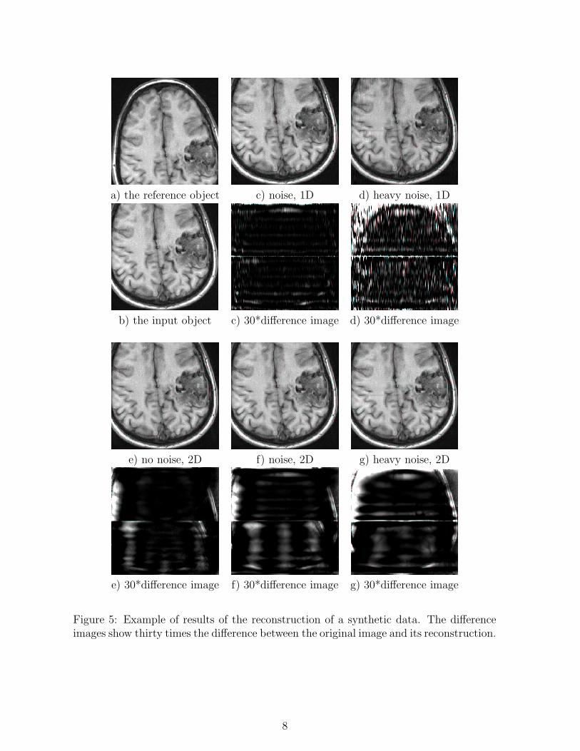
a) the reference object c) noise, 1D d) heavy noise, 1D

b) the input object c) 30*difference image d) 30*difference image

e) no noise, 2D f) noise, 2D g) heavy noise, 2D

e) 30*difference image f) 30*difference image g) 30*difference image

Figure 5: Example of results of the reconstruction of a synthetic data. The differenceimages show thirty times the difference between the original image and its reconstruction.

8

smoothly also along the x direction. The solution is to utilize this property and to usea 2D grid of B-splines. This is faster, more robust to noise and takes advantage of thesmoothness of the sensitivity in the x direction. The coefficients are estimated at onceproducing no discontinuities in the x direction.

The coefficients α are approximated by a 2D grid of B-splines

αml(x,y) =

Ni∑

i=1

Nj∑

j=1

gmijl βp( y

hy− i) βp( x

hx− j) =

Ni∑

i=1

Nj∑

j=1

gmijl ϕYi (y) ϕX

j (x), (8)

where Nj is the number of splines used in the x direction. The notation for the B-splinebasis in the x and y direction is shortened to ϕX

j (x) and ϕYi (y).

The error (6) then changes to

em =

Ny

M∑

y=1

Nx∑

x=1

∥

∥

∥

∥

∥

∥

L∑

l=1

Ni∑

i=1

Nj∑

j=1

(gmijl ϕi(y) ϕj(x) Sl(x,y+mNyM

)) − S(x,y+mNyM

)

∥

∥

∥

∥

∥

∥

2

+∑

m′ 6=m

Ny

M∑

y=1

Nx∑

x=1

∥

∥

∥

∥

∥

∥

L∑

l=1

Ni∑

i=1

Nj∑

j=1

gmijl ϕi(y) ϕj(x) Sl(x,y+m′ NyM

)

∥

∥

∥

∥

∥

∥

2

. (9)

The computation then continues in the same manner as in the 1D case and yieldsthe following equations after setting the derivatives to zero

∑

y,x

ϕYi ϕX

j S∗l (m) S(m) =

∑

i′,j′,l′

gmi′j′l′

∑

y,x

ϕYi ϕY

i′ ϕXj ϕX

j′

M−1∑

m′=0

Sl′ (m) S∗l (m).

The shorter notation is also used regarding the changes to 2D. ϕYi (y) → ϕY

i , Sl(x,y+mNyM

) →Sl(m).

Example of the results on a real and a synthetical data are shown in Figures 4 and 5.

4 Implementation

The proposed methods were implemented in Matlab. This programming language waschosen because of its support for computations with matrices. It is easy to implementand test the algorithm in this programming language. However, the speed of Matlabis not optimal. Therefore some of the routines should be rewritten in a more efficientlanguage (for example C) before using the algorithm in practice.

There are two main functions implemented. The first is the function that estimatesthe coefficients. As an input, it takes reference images (full-FOV body-coil image andfull-FOV array-coil images) stored in a raw format. The output of this function is aMatlab matrix that contains the coefficients α. The second function is the reconstructionfunction. It takes aliased array-coil images and the coefficients α as an input. It returnsthe reconstructed image stored in matrix or save the image in a standard image format.

5 Experiments

The methods presented in Sections 3.2 and 3.3 were tested on synthetic and real data.

9

5.1 Synthetic data

Two images of a brain slice were chosen for this purpose. The first brain image was takento be the reference body-coil image. The array-coil images were created by modifying thefirst brain image by sensitivity maps. A synthetic sensitivity maps (real - not complex -maps) were used. Next, the Gaussian noise was added independently to each referenceimage to simulate the presence of noise in the receiver coils.

Input images were created from both images of a brain slice. The same sensitivitymaps and different images were used for the reconstruction to ensure that the recon-struction is working for any image acquired using the same sensitivity maps. A Gaussiannoise was added only to reference images to affect the estimation, not the reconstruction.

The reconstruction coefficients were estimated on the first image (see Figure 5a) andused for reconstructing both first and second image (see Figure 5b). Reconstruction ofthe same images that were used as a reference image is close to ideal and there are nomajor errors.

The error becomes visible when reconstructing the second image. Both 1D and 2Dreconstructions introduce minor errors for reconstruction without noise (see Figure 5e).1D reconstruction has slight problems with estimating coefficients in the places whereis no object and where is a high presence of noise. This can be observed in Figure 5das discontinued lines in the top left of the image. 2D estimation of coefficients is morerobust to this phenomena and the estimation is also robust to noise. In Figures 5f and5g we can see that the error is not getting much worse with presence of noise in referenceimages. The reconstruction is however getting worse for the 1D case (see Figure 5d).

5.2 Real data

The methods were tested on an image of a vessel phantom (see Figures 1, 4a). The coef-ficients α were estimated from a body-coil image and a set of unaliased array-coil images.A set of aliased array-coil images of the same object was used for the reconstruction.

The reconstruction is good even with a low number of splines (see Figures 4b, 4c).Artifacts visible on the top and in the center of the images are caused by a part of thephantom that was not visible in the reference images, but is visible in the input images.

Adding more splines brings only a minor improvement in accuracy and artifact re-duction (see Figure 4d). However, it increase the reconstruction time.

6 Conclusion

We had proposed and implemented a pMRI reconstruction algorithm. It estimates thereconstruction coefficients directly from the reference images without estimating thesensitivity maps first. It uses a grid of B-splines to approximate the reconstructioncoefficients. This makes the estimation more robust to noise in reference images. Thenumber of parameters of the reconstruction is reduced. This increases the speed ofthe reconstruction. Since the sensitivities are changing smoothly, we did not observeany adverse effects of the smaller number of B-spline coefficients on the quality of thereconstructed images. There is also no restriction on the coil configuration as in SMASH(of course, assuming invertibility (3)).

10

7 Future work

1. Estimating α from low resolution reference scans. Currently we are using referenceimages of the same resolution as the input images. However, it should be sufficientto use reference images with a lower resolution to estimate the reconstructioncoefficients.

2. Variable density sampling in the k-space. It is possible to sample with variabledensity in k-space. If we do not skip lines in the center of the k-space, but onlyouter lines, we get simultaneously a low-resolution full-FOV image and also afull-resolution reduced-FOV image. The first image can be used to estimate thecoefficients to reconstruct the full-resolution image. The advantage is that thereference and input images are taken at the same time. This is also done in thecurrently available methods - mSENSE, GRAPPA [2].

3. Speeding up the estimation. Speed is the crucial step in pMRI. We will enhance thereconstruction speed by improving the implementation, by rewriting to it C++,. . .

4. Model with noise. We will make a model that takes into account the noise in thereceiver coils and will try to remove the effect of noise in the estimation and thereconstruction.

5. 3D model. After the method will be working fine in 2D it is planned to createa method that will estimate the reconstruction coefficients in 3D. It will allowreconstructing of objects in an arbitrary plane.

6. Comparison. The method should be quantitatively compared with the methodsimplemented in the Siemens Symphony MRI scanner.

References

[1] Mark A. Griswold, P. M. Jakob, M. Nittka, J. W. Goldfarb, and A. Haase. VD-AUTO-SMASH imaging. Magnetic Resonance in Medicine, 45(6):1066–74, 2001.

[2] Mark A. Griswold, Peter M. Jakob, Robin M. Heidemann, Mathias Nittka, VladimirJellus, Jianmin Wang, Berthold Kiefer, and Axel Haase. Generalized autocalibrat-ing partially parallel acquisitions (GRAPPA). Magnetic Resonance in Medicine,47:1202–10, 2002.

[3] Charles A. McKenzie, Ernest N. Yeh, Michael A. Ohliger, Mark D. Price, andDaniel K. Sodickson. Self-calibrating parallel imaging with automatic coil sensitivityextraction. Magnetic Resonance in Medicine, 47:529–38, 2002.

[4] Klass P. Pruessmann, Markus Weiger, Markus B. Sheidegger, and Peter Boesiger.SENSE: Sensitivity Encoding for Fast MRI. Magnetic Resonance in Medicine,42:952–62, 1999.

[5] Robert C. Smith and Robert C. Lange. Understanding magnetic resonance imaging.CRC Press LCC, 1998.

[6] Daniel K. Sodickson. Tailored SMASH image reconstruction for robust in vivoparallel MR imaging. Magnetic resonance in medicine, 44:243–51, 2000.

11

[7] Daniel K. Sodickson and W. Manning. Simultaneous acquisition of spatial harmon-ics (SMASH): fast imaging with radiofrequency coil arrays. Magnetic Resonance in

Medicine, 38:591–603, 1997.

[8] Michael Unser. Splines - A perfect fit for signal and image processing. IEEE Signal

processing magazine, pages 22–38, November 1999.

[9] Marinus T. Vlaardingerbroek and Jacques A. Boer. Magnetic Resonance Imaging:

Theory and Practice. Springer-Verlag, 1996.

[10] Y. Wang. Description of parallel imaging in MRI using multiple coils. Magnetic

Resonance in Medicine, 44(3):495–9, 2000.

12